Embed Size (px)
Citation preview

Advanced Predictive Modeling Fall 2015 Term Paper
Classifying Readmissions based on parameters of a Diabetic patient encounter
by Jace Barton, Zahref Beyabani, Anagh Pal, Dhwani Parekh, and Mayur Srinivasan
Abstract
Readmission rates in hospitals are a key indicator on quality of patient care and a clear
indication of total cost or inconvenience related to the treatment. Patients with serious medical
conditions such as diabetes mellitus are key drivers of readmission rates owing to the complexity
of their illness. Therefore, being able to predict based on certain features whether or not a patient
will need readmission can help doctors and hospitals provide better care initially and not get
financially penalized under Obamacare’s readmission policy. Our project explores various
classification techniques to achieve a prediction of whether or not a patient will be readmitted.
The results obtained are not too promising however, as evidence towards the predictors available
not encompassing the true cause of readmission keeps presenting itself throughout our
endeavors.
Introduction
National Diabetes Statistics Report[1], 2014 by Centers for Disease Control and
Prevention mentions that 29.1 million people or 9.3% of the U.S. population have diabetes out of
which 8.1 are undiagnosed. A separate study[2] cited by the WHO states that these numbers are
only going to increase and a systemic but controllable disease like Diabetes is going to be the 7th
leading cause of death by 2030. Estimates show that $245 billion is spent in the US on diabetes
related ailments as a part of direct and indirect costs(includes disability, work loss and premature
death). A hospital’s readmission rate is a significant and a direct contributor to total medical
expenditure and is an apparent indicator of the quality of care provided. Chronic, debilitating,
and severe medical conditions such as diabetes are connected with higher risks of hospital
readmission. Our project’s aim was to utilize the diabetes dataset available on the UCI machine
learning repository, and apply concepts learnt in class to determine if a prediction on whether or
not a patient would be readmitted could be made based on data collected on in-patient diabetic
encounters. From a treatment perspective, being able to tell whether or not a patient would be
readmitted from the start could mean a better focus on the patient to prevent the readmission,
consequently resulting in a better health outcome. From a fiscal standpoint, it is cheaper for both
the patient and the hospital if the readmission rate is low, as the hospital does not need to expend

Advanced Predictive Modeling Fall 2015 Term Paper
already scarce capacity multiple times, if they can succeed in appropriate treatment the first time.
Finally, from an Obamacare compliance outlook, it is better for the hospital to have low
readmission rates as penalties exist for hospitals with high readmission rates. We performed
some basic data treatment, and proceeded to split it into a training and test set before proceeding
with the application of predictive modeling.
Data and Pre-Processing
This original data used the Health Facts database (Cerner Corporation, Kansas City, MO),
a national data warehouse that collects comprehensive clinical records across hospitals
throughout the United States. This contained data systematically collected 1from participating
institutions electronic medical records and includes encounter data (emergency, outpatient, and
inpatient), provider specialty, demographics (age, sex, and race), diagnoses and in-hospital
procedures documented by ICD-9-CM codes, laboratory data, pharmacy data, in-hospital
mortality, and hospital characteristics. However, all data were de-identified in compliance with
the Health Insurance Portability and Accountability Act of 1996. The data spanned 10 years
(1999–2008) of clinical care at 130 hospitals and integrated delivery networks throughout the
United States: Midwest (18 hospitals), Northeast (58), South (28), and West (16).
The data available (which was used) described unique individual patient encounters that resulted
in a primary, secondary or additional secondary diagnosis as being diabetic related. Information
on patient demographics such as age, race, and gender were available, in addition to their test
results, medications, and finally what we picked as a response variable: whether or not the
particular patient was readmitted. The dataset subscribes to the following assumptions:
- It was an inpatient (Hospital admission) encounter and not just a physician / clinic visit
- The encounter was a strictly in-patient encounter lasting between one and fourteen days
- The encounter resulted in an ICD9 code pertaining to diabetes to be entered as a primary,
secondary or additional secondary diagnosis.
- One or more laboratory tests were performed during this patient’s admission and/or stay [1] http://www.cdc.gov/diabetes/pubs/statsreport14/national-diabetes-report-web.pdf [2] http://www.who.int/mediacentre/factsheets/fs312/en/

Advanced Predictive Modeling Fall 2015 Term Paper
- Medications were administered / prescribed during the encounter.
Some data preprocessing was required to align the data with our aims for this project, the main
one being coding the response variable to match the stipulation of the Obamacare readmission
penalty policy. The policy defines a readmission as one where the patient was readmitted to the
hospital within 30 days of the first admission. The dataset consisted of more granular data
describing readmissions; hence we simplified it to indicate whether or not a readmission
occurred within 30 days. Other aspects of preprocessing were to scale numeric variables to have
a zero mean and unit variance, and imputing the patient race when it was not available utilizing
previous encounter data. Additional pre-processing or re-encoding of certain variables was
required for particular models, and the measures undertaken are described in the specific sections
of this paper that pertain to those models.
Exploratory Data Analysis
Prior to performing any statistical modeling or training classifiers, it is a good idea to get
to know and get familiarized with the underlying data. Included below are some of our
exploratory data analysis that details what kind of data exists, and some preliminary insights.

Advanced Predictive Modeling Fall 2015 Term Paper
Fig 1. Data Description

Advanced Predictive Modeling Fall 2015 Term Paper
Fig 2. Response variable coding
Fig 3. Encounters by age
Fig 4. Patient Demographics

Advanced Predictive Modeling Fall 2015 Term Paper
Fig 5. Number of days spent as in-patient by encounters
Association Analysis of Diagnosis Feature for Level Reduction
One of the challenges that we faced quite early into our model development was the
number of levels for certain features. Features with a very high number of levels led to a
significant increase in computation time as well as a huge loss in interpretability of the model.
This resulted in important features being sidelined and biased, while the model results were far
from explicable. We also noticed that many of the models developed were susceptible to the
number of levels in the feature space, and hence reducing the number of levels for certain
features became an operational requirement for us. Major features that exhibited this problem
were ‘medical speciality’ (with over 80 levels) and ‘diagnosis’ variables (with over 800 levels
overall)
The levels of ‘medical speciality’ feature were reduced manually, using our best judgement of
medical specialties that are similar or are highly under-represented. For example, the following
set of specialties were grouped under one ‘Pediatrics’ specialty
Similarly, we found quite a few groups within ‘Surgery’ and ‘Obsterics’. Hence, we were able to
reduce the number of levels for ‘medical specialty’ to around 27 levels
PediatricsPediatrics-‐AllergyandImmunologyPediatrics-‐CriticalCarePediatrics-‐EmergencyMedicinePediatrics-‐EndocrinologyPediatrics-‐Hematology-‐OncologyPediatrics-‐InfectiousDiseasesPediatrics-‐NeurologyPediatrics-‐Pulmonology

Advanced Predictive Modeling Fall 2015 Term Paper
We were faced with a much bigger challenge with respect to the ‘diagnosis’ feature as explained
below.
Diagnosis Variables
The diagnosis variables in our data were spread across three features:
The Primary diagnosis, Secondary diagnosis, Additional Secondary Diagnosis (coded as first
three digits of ICD9)
Even though all the data we have here is a diabetes related encounter, diabetes may not be the
primary, secondary, or additional secondary diagnosis in most encounters. These are the cases
where diabetes was one of the many diagnoses, but do not feature in the ‘Top 3’
The challenge with using the diagnosis variable as-is, is that across primary, secondary, and
additional secondary diagnoses, we have close to 800 unique levels. This leads to a breakdown
of the models and major loss of interpretability as discussed earlier
Options
With the given scenario, we approached the problem of high ‘vertical’ dimensionality in 2
ways:
1. Convert diagnosis to a binary feature
We could convert the diagnosis variables where diabetes (ICD9 code = 250) is either primary,
secondary, or additional secondary to a ‘positive class’ of ‘Diabetes Important Diagnosis’. The
negative class will comprise of encounters where diabetes does not feature in any of the three
important diagnosis variables
One of the downfalls of this approach is the loss of valuable information in the form of diagnoses
other than diabetes. We have observed empirically that certain lifestyle diseases occur in groups,
and hence we should ideally move towards an approach that takes this inherent association into
consideration
2. Convert diagnosis into a metric measuring importance of diabetes (including association)
As discussed before, the association between diagnosis is an important factor that we should
ideally be incorporating as we resolve the high dimensionality issue with the diagnosis variables.
Primary Diagnosis Secondary Diagnosis Additional Secondary Diagnosis
Advanced Predictive Modeling Fall 2015 Term Paper
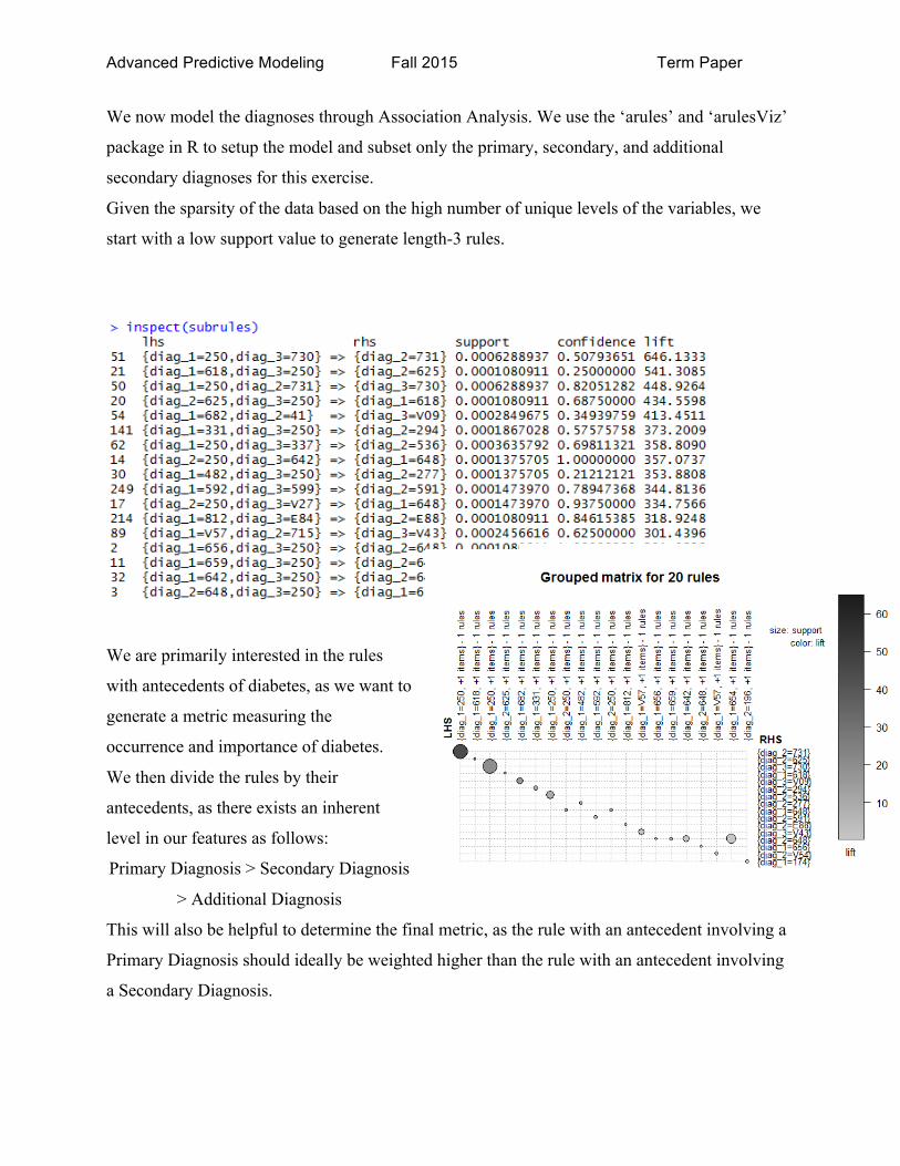
We now model the diagnoses through Association Analysis. We use the ‘arules’ and ‘arulesViz’
package in R to setup the model and subset only the primary, secondary, and additional
secondary diagnoses for this exercise.
Given the sparsity of the data based on the high number of unique levels of the variables, we
start with a low support value to generate length-3 rules.
We are primarily interested in the rules
with antecedents of diabetes, as we want to
generate a metric measuring the
occurrence and importance of diabetes.
We then divide the rules by their
antecedents, as there exists an inherent
level in our features as follows:
Primary Diagnosis > Secondary Diagnosis
> Additional Diagnosis
This will also be helpful to determine the final metric, as the rule with an antecedent involving a
Primary Diagnosis should ideally be weighted higher than the rule with an antecedent involving
a Secondary Diagnosis.
Advanced Predictive Modeling Fall 2015 Term Paper
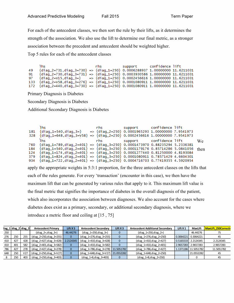
diag_1 diag_2 diag_3 Antecedent Primary Lift X 5 Antecedent Secondary Lift X 3 Antecedent Additional Secondary Lift X 1 MaxLift MaxLift_250Correction250 {diag_2=,diag_3=} 46.44276 {diag_1=250,diag_3=} 0 {diag_1=250,diag_2=} 46.44276 75276 250 255 {diag_2=250,diag_3=255} 0 {diag_1=276,diag_3=255} 0 {diag_1=276,diag_2=250} 0.3064221 0.3064221 45410 427 428 {diag_2=427,diag_3=428} 2.2124345 {diag_1=410,diag_3=428} 0 {diag_1=410,diag_2=427} 0.5165533 2.2124345 2.2124345410 401 582 {diag_2=401,diag_3=582} 0 {diag_1=410,diag_3=582} 0 {diag_1=410,diag_2=401} 2.9657283 2.9657283 2.9657283786 427 278 {diag_2=427,diag_3=278} 0 {diag_1=786,diag_3=278} 11.5051782 {diag_1=786,diag_2=427} 1.1371186 11.5051782 11.5051782648 250 V27 {diag_2=250,diag_3=V27} 0 {diag_1=648,diag_3=V27} 21.0552282 {diag_1=648,diag_2=250} 21.0552282 458 250 403 {diag_2=250,diag_3=403} 0 {diag_1=8,diag_3=403} 0 {diag_1=8,diag_2=250} 0 45
For each of the antecedent classes, we then sort the rule by their lifts, as it determines the
strength of the association. We also use the lift to determine our final metric, as a stronger
association between the precedent and antecedent should be weighted higher.
Top 5 rules for each of the antecedent classes
Primary Diagnosis is Diabetes
Secondary Diagnosis is Diabetes
Additional Secondary Diagnosis is Diabetes
We
then
apply the appropriate weights in 5:3:1 proportion, for the three antecedent classes on the lifts that
each of the rules generate. For every ‘transaction’ (encounter in this case), we then have the
maximum lift that can be generated by various rules that apply to it. This maximum lift value is
the final metric that signifies the importance of diabetes in the overall diagnosis of the patient,
which also incorporates the association between diagnoses. We also account for the cases where
diabetes does exist as a primary, secondary, or additional secondary diagnosis, where we
introduce a metric floor and ceiling at [15 , 75]

Advanced Predictive Modeling Fall 2015 Term Paper
Cost Penalty Matrix for Readmission from Diabetic Encounters
For a binary classifier like most of the models we’ll develop, the error or
misclassification can be very costly. The cost of misclassification is not incorporated in the
model development in its general form, but the impact of cost can be big enough to influence the
parameter thresholds significantly. As such, the incorporation of misclassification costs changes
the classification process into an optimization problem, wherein the cost minimization is the
objective, and model accuracy is a consequence of this optimization.
For our problem, the cost of misclassification can be illustrated as below:
Let’s explore each of the costs one-by-one:
1. Benefit of predicting a right readmission
Most U.S. hospitals will get less money from Medicare in fiscal 2016 because too many patients
return within 30 days of discharge. The readmissions program, created under the Affordable
Care Act, initially evaluated how often patients treated for heart attack, heart failure and
pneumonia had to return to the hospital within 30 days of discharge. Facilities with too high a
readmission rate saw their Medicare payments docked up to 1% in fiscal 2013. The financial
stakes increased to a 2% reduction in fiscal 2014[3]
Hence, assuming that a hospital has the resources to reduce or control readmission based on an
accurate prediction of readmissions of its patients, we can say that hospitals can save an amount
equivalent to the Medicare penalty discussed above. To do this, we find the value of the penalty
through the average Medicare coverage per capita below:
𝑉𝑎𝑙𝑢𝑒 𝑜𝑓 𝑃𝑒𝑛𝑎𝑙𝑡𝑦 𝑆𝑎𝑣𝑒𝑑 =𝑇𝑜𝑡𝑎𝑙 𝑀𝑒𝑑𝑖𝑐𝑎𝑟𝑒 𝑆𝑝𝑒𝑛𝑑𝑖𝑛𝑔 ($)𝑀𝑒𝑑𝑖𝑐𝑎𝑟𝑒 𝐶𝑜𝑣𝑒𝑟𝑎𝑔𝑒 (𝑢𝑛𝑖𝑡𝑠) ∗ 𝑃𝑒𝑛𝑎𝑙𝑡𝑦 (%)
From [1], Total Medicare Spending = $505 billion and from [2], total Medicare coverage = 5.23
million. We also saw above that the Penalty imposed is up to 1% of the Medicare $ value
Therefore,
Readmission No Readmission
Readmission1. Benefit of predicting a right
readmission
2. Cost incurred by hospital when the model predicts 'no readmission' but a
patient is readmitted
No Readmission3. Cost incurred when a patient isn't readmitted even though the model predicts s/he will
4. Benefit of predicting a right 'no readmission'
PREDICTED CLASS
ACTU
AL CLASS
COST PENALTY MATRIX

Advanced Predictive Modeling Fall 2015 Term Paper
𝑉𝑎𝑙𝑢𝑒 𝑜𝑓 𝑃𝑒𝑛𝑎𝑙𝑡𝑦 𝑆𝑎𝑣𝑒𝑑 = −$𝟗𝟔.𝟓𝟔 (negative because this is a benefit, and not a cost)
2. Cost incurred by hospital when the model predicts 'no readmission' but a patient is
readmitted
The crux of this entire exercise is to reduce this particular cost – when a model predicts that the
customer is very unlikely to be readmitted, but a patient does have a readmission encounter. This
incurs a huge cost for the hospital, as a) the readmission is unplanned and expensive b) it denies
medical care to other unplanned patients where there was no way to predict the admission.
Readmission costs are well documented as it is one of the largest sources of avoidable risk/cost
for hospitals. For our problem, we can restrict ourselves to the readmission costs of diabetic
encounters, as they constitute about 4% of readmissions [4] that make up the average
readmission costs in the report. We can define the False Negative Class rate as follows:
𝐶𝑜𝑠𝑡 𝑜𝑓 𝑝𝑟𝑒𝑑𝑖𝑐𝑡𝑖𝑛𝑔 "no readmission" 𝑤ℎ𝑒𝑛 "𝑎𝑑𝑚𝑖𝑠𝑠𝑖𝑜𝑛"
= 𝑇𝑜𝑡𝑎𝑙 𝐶𝑜𝑠𝑡 𝑜𝑓 𝐷𝑖𝑎𝑏𝑒𝑡𝑒𝑠 𝑅𝑒𝑎𝑑𝑚𝑖𝑠𝑠𝑖𝑜𝑛
𝑇𝑜𝑡𝑎𝑙 𝐷𝑖𝑎𝑏𝑒𝑡𝑒𝑠 𝑅𝑒𝑎𝑑𝑚𝑖𝑠𝑠𝑖𝑜𝑛𝑠
From [4], we can plug-in the values to find the following value of misclassification cost
𝐶𝑜𝑠𝑡 𝑜𝑓 𝑝𝑟𝑒𝑑𝑖𝑐𝑡𝑖𝑛𝑔 no readmissio 𝑤ℎ𝑒𝑛 admission = $𝟏𝟎,𝟓𝟗𝟎.𝟕𝟐
3. Cost incurred when a patient isn't readmitted even though the model predicts s/he will
It is in the best interest of a hospital to know exactly if a patient will be readmitted. The cost to
control the risk is very high, but the value of perfect information about a patient’s readmission
can tell us a lot about the costs of preparing for a patient readmission which might go to waste
due to misclassification. A False Positive classification can hence, lead to a cost of missed
opportunity and excess capacity. We can gauge the value of this cost by exploring the average
medical costs for diabetes diagnosis.
From [5], we can observe that the total cost of Diabetes diagnosis is well documented. Our focus
is on the tangible medical costs which is the biggest part of the cost. We also observe that the
medical costs involve patient costs as well. But, for our problem, we are primarily concerned
with the costs incurred by hospitals in preparing for a diabetic encounter/diagnosis. This is
illustrated by the 60% share of hospital costs to the total medical cost incurred by a hospital. As
we are comparing the costs at a per capita level, we normalize this value with the total number of

Advanced Predictive Modeling Fall 2015 Term Paper
diabetes patients in a year from [6]. The cost of False Positive class misclassification can then be
given by:
𝐶𝑜𝑠𝑡 𝑜𝑓 𝑝𝑟𝑒𝑑𝑖𝑐𝑡𝑖𝑛𝑔 admission" when "𝑛𝑜 𝑟𝑒𝑎𝑑𝑚𝑖𝑠𝑠𝑖𝑜𝑛"
= 𝑇𝑜𝑡𝑎𝑙 𝑀𝑒𝑑𝑖𝑐𝑎𝑙 𝐶𝑜𝑠𝑡𝑠 𝑜𝑓 𝐷𝑖𝑎𝑏𝑒𝑡𝑒𝑠 ∗% ℎ𝑜𝑠𝑝𝑖𝑡𝑎𝑙 𝑐𝑜𝑠𝑡𝑠
# 𝑜𝑓 𝑑𝑖𝑎𝑏𝑒𝑡𝑒𝑠 𝑝𝑎𝑡𝑖𝑒𝑛𝑡𝑠
Therefore,
𝐶𝑜𝑠𝑡 𝑜𝑓 𝑝𝑟𝑒𝑑𝑖𝑐𝑡𝑖𝑛𝑔 admission" when "𝑛𝑜 𝑟𝑒𝑎𝑑𝑚𝑖𝑠𝑠𝑖𝑜𝑛" = $𝟑,𝟎𝟏𝟕.𝟏𝟒
4. Benefit of predicting a right 'no readmission'
The benefit to predicting a right ‘no readmission’ is almost negligible, as most cases are ‘no
readmission’ and the hospital does not gain significant value from this information. More
importantly, this classification predicts the majority class and does not have any direct link to
any of the major Medicare policy decisions that might impact hospitals substantially
To summarise, the cost penalty matrix looked at the factors that influence various classification
and misclassification costs. The cost penalty matrix helps us to remodel the problem as a ‘cost
reduction’ optimization model, which is especially useful in a highly imbalanced data
environment. The cost penalty matrix helps us in identifying probability thresholds that are more
sanguine and appropriate to evaluate our models
Logistic Regression
Readmission for diabetic patient encounters can be modeled as a probability based on the
given inputs. As such, instead of a classification model, we can aim to predict the probability of
readmission using a logistic regression model. A probability model will help us tweak the final
thresholds at various levels. This is desirable because we have already established that the data is
highly imbalanced, and hence would require further inspection in the classification results.
A logistic regression model is defined as:
ln𝐹(𝑥)
1− 𝐹(𝑥) = 𝛽! + 𝛽!𝑥
Readmit NoAdmitReadmit -‐96.56$ 10,590.72$ NoAdmit 3,017.14$ -‐$
Predicted
Actual
Cost Matrix

Advanced Predictive Modeling Fall 2015 Term Paper
where F(x) is interpreted as the probability of the dependent variable equaling a "success" or
"case" rather than a failure or non-case. ‘x’ represents the input, independent variable space.
Data Preparation
For our problem, the dependent variable is the “success” or “failure” of readmission
based on the variable space that has been described before. Logistic regression has the ability to
parse both continuous and categorical variables, the latter incorporated into the model through
dummy encoding. As most of the variables in the input space are categorical and dummy
encoding is easier to implement in R, we use the statistical software R to model and test the
logistic regression model on the data using standard R packages such as ‘glm’ and explore
regularization through ‘glmnet’
The input data was processed to account for levels, and appropriate features were changed into
factors. We replace the diagnosis variables with the Diabetes Diagnosis metric developed earlier.
We also eliminate variables that do not show any variability, as it would adversely affect the
performance of the logistic regression model.
The processed data is first divided into test and train, maintain the positive:negative class balance
as in the original data. This is done to ensure that the model predictability is done on a robust
test, controlling for any other factors except the viability of the model.
Model Setup and Results
We first use the glm() package on R to fit the model on training data. This requires a
transformation of the input space into a data matrix. We also have to eliminate any features that
do not have any variability – in our model, it implies that some categorical variables with only 1

Advanced Predictive Modeling Fall 2015 Term Paper
level have to be removed before running the model, as it does not have any predictive power in
the model, and leads to matrix inversion error during the coefficient estimation.
One learning outcome from the results above is that the model contains many features that are
insignificant and/or are of little consequence (miniscule coefficients). Also, the nature of feature
vectors will tend to inflate certain coefficients. This leads us to explore regularization methods
that achieve feature selection and/or feature control (through control of inflated coefficient
values)
Regularization
We now setup a new model with Lasso regularization using glmnet() package on R.
Lasso regularization is run on glmnet() using the alpha parameter equal to 1. The default setting
of 10-fold cross validation is used in this case.
The results from Lasso are shown below. We first determine the optimum regularization
parameter (lambda) that minimizes the Mean Square Error across the cross validation through
the graph below.
We observe that the Lasso Regularization penalty factor for the lowest MSE reduces the
coefficients for almost all of the features. This implies that the predictive power of most features
is very low. The best model fit (lowest MSE) is obtained when only 2 features are used.
At this stage, we could look at a penalty factor in the vicinity of the above factor, or a penalty
factor that achieves a low (but not the lowest) MSE, but still retain a reasonable number of
features to work with. We could also look at another kind of regularization – Ridge, to abandon
feature selection and focus just on the control of large coefficients from the original model.

Advanced Predictive Modeling Fall 2015 Term Paper
We now setup a new model with Ridge regularization using glmnet() package on R using the
alpha parameter as 0. The default setting of 10-fold cross validation is used in this case.
The results from Ridge are shown below. We first determine the optimum regularization
parameter (lambda) that minimizes the Mean Square Error across the cross validation through
the graph below
Based on the values of the coefficients from Ridge regularization, the important variables/levels
in the model are as below:
Higher the chance of readmission when
Feature Level Significant
visit_count More the number of encounters recorded in data
age 80-90 and surprisingly, 20-30 as well
admission “transfer from a hospital” or “emergency room”
admission source “transfer from inpatient” or “court/law enforcement”
discharge disposition “expected to return” or “discharged within
institution”
medical speciality ‘hematology’ and ‘oncology’
Hb1ac No A1c test was done
medications when repaglinide and insulin dosage was increased

Advanced Predictive Modeling Fall 2015 Term Paper
Test Performance
Before we can test the model we have just developed, it is important to address the
imbalance in classes in the data. This affects the model performance considerably, as the
threshold for class prediction can no longer remain at the default value of 50%.
We have explored two ways in which we determine an appropriate threshold for this exercise:
a) Manually inspect various values of threshold for a good mix of accuracy and recall
b) Use the cost penalty matrix to determine a good threshold
We now test the Ridge regularized model on the test data that was prepared earlier. The data
preparation for train and test was done together to ensure that there are no dimensional errors
during model testing.
For a classification model such as the logistic regression model just developed, one of the best
ways to gauge the model performance is to observe the confusion matrix and ROC curve. A
good model fit is where the area under curve is high, which leads to maximum accuracy. The
ROC curve generated for a threshold value of 0.3 is shown below. As indicated in the diagram,
we are primarily interested in the low ‘false positive rate’ region of the graph, due to the extreme
bias in classes in the data
We briefly shift our focus to assigning a new
threshold based on the cost penalty matrix. Our
hypothesis is that we should aim to bring the cost
of predicting admission or no readmission to as close as possible, without affecting accuracy
considerably. We revisit the cost matrix below:

Advanced Predictive Modeling Fall 2015 Term Paper
Suppose that the probability threshold (probability of actual readmission) is p
Then, cost of predicting readmission = cost of predicting admission is given by:
-96.56p + 3,017.17(1-p) = 10,590.72p
Hence, p = 0.22
We recalibrate our model to reflect this new threshold and obtain the following results (on next
page)
We see that our new model (threshold) obtains a healthy accuracy of 88.88% while also
optmising the cost function based on a previously defined cost penalty matrix. This motivates us
to go ahead with this model as the final model out of the Ridge regularization of logistic
regression
Artificial Neural Network - Multilayer Perceptron
A Multilayer perceptron is used to improve on the classification accuracy of logistic
regression and also because they work particularly well for:
- Capturing associations or discovering regularities within a set of patterns
- Cases where the volume, number of variables or diversity of the data is very great
Readmit NoAdmitReadmit -‐96.56$ 10,590.72$ NoAdmit 3,017.14$ -‐$
Predicted
Actual
Cost Matrix

Advanced Predictive Modeling Fall 2015 Term Paper
- The relationships between variables are vaguely understood
- The relationships that are difficult to describe adequately with conventional approaches
Because of the lack of our domain expertise in the healthcare, Multilayer perceptron is a great
tool because there are very specific details on medications provided, lab tests performed etc.
which are difficult to use without.
A model on the pre-processed data without any further processing was attempted which failed
due to close to 800 levels in the three diagnoses variable which resulted in more than 2400
dummy variables and would be practically possible only on a server. To reduce the number of
levels in the categorical variables, the data was converted in the following two ways:
- Physician specialty was consolidated to lower number of levels (because there were
variation in denoting the same specialty)
- The Diagnoses was reduced to a binary variable which denoted the absence/presence of
diabetes diagnoses
The representation of the diagnoses to a binary variable obviously does lead to loss of
information but this is needed to reduce the vertical dimensionality which was impeding the
model building exercise. A work around - association analysis of the diagnoses can be used to
retain the information in lower dimensions has been explained in a later section. The model was
trained on a down sampled version of the training set to ensure better results because the data is
imbalanced (with only 11% of readmissions).
A MLP (Multilayer Perceptron) has a couple of knobs that can be tweaked to obtain the best
performing model – the number of iterations (epochs), the number of nodes and the number of
layers. The model was first tested on an artificially balanced tests set to understand the
performance of the model. The results are shown as below:
The low accuracy rate (60.4%) of the model even on a balanced data set can signify any one of
the two things:
- The model is not accurate enough
- There are missing factors/variables in the data (based on studies socio economic status and
things like availability of a car are important factors
The next step is to understand the best parameters for which predictions are the best on a
imbalanced test set which is a simulation of the real life scenario. Based on the random training

Advanced Predictive Modeling Fall 2015 Term Paper
set that was chosen some of the variables like examide, citoglipton, acetohexamide, troglitazone,
glimepiride.pioglitazone, metformin.rosiglitazone and metformin.pioglitazone were removed
because they do not show any variation/change in the sample.
N_Iter
Number of hidden units
Accuracy AUC
500 25 57.16% 0.601
500 30 56.80% 0.586
500 40 70.66% 0.604
500 50 70.65% 0.604
500 70 34.60% 0.429
750 25 56.63% 0.599
1000 20 58.27% 0.603
1000 25 55.70% 0.597
1500 50 30.13% 0.438
400 40 58.85% 0.630
300 40 33.90% 0.432
600 40 37.34% 0.432
1000 40 0.5667 0.592
As seen from the model none of the models are performing particularly well even after tweaking
the parameters. It can be seen that for number of iterations/epochs equal to 500, the AUC and
accuracy increases. This can be attributed to reduction in bias, but increasing the number of
hidden nodes further increases the variance, hence the over fitting the data and performing
poorly on the test/holdout set. Similarly while keeping the number of hidden units constant at 40,
it is noticed that accuracy and AUC is highest for n_iter= 500. Increasing the number of epochs
from 500 increases the variance, resulting in overfitting of the data.

Advanced Predictive Modeling Fall 2015 Term Paper
One of the reasons, the models are not robust enough might because the number of level for the
diagnoses variable was reduced drastically from 800 to 2 each. To try to faithfully represent the
information captured in these variables, the binary variables are replaced by the association score
(explained in the other section). The inclusion of the association variable or adding another layer
of hidden units does not improve the performance in terms of predictions. These are strong
pointers to the fact that the data has missing variables which are crucial to the understanding
patterns within patient re-admissions.
Performance Parameters post inclusion of association variables of diagnoses
N_iter
Number of hidden
units
Accurac
y AUC
200 40 60.28% 0.6542
300 40 68.29% 0.6797
350 40 67.55% 0.6721
400 40 61.59% 0.6544
500 40 41.54% 0.4515
700 40 41.17% 0.4502
300 50 66.59% 0.6361
400 50 60.35% 0.6739
500 50 34.54% 0.3921

Advanced Predictive Modeling Fall 2015 Term Paper
Support Vector Machine Approach to Classification
Our next thought was to use a support vector machine to classify patients. We thought
this approach would work well because we know support vector machines work well with high-
dimensional data and they are also able to handle imbalanced data with respect to the
classification variable of interest. We also knew that SVMs performed better for many tasks
when compared to other models.
We ran into several difficulties when attempting to utilize SVMs with our data however. The
first issue was transforming all of the categorical variables into dummy variable columns so they
could be used in the analysis. While not technically complex to accomplish, given how many
rows there were the explosion in columns led to a matrix too large for the SciKitLearn SVC
package in Python to handle.
We solved this problem in three ways. First, as discussed earlier, we changed our approach to
diagnosis classification to result in a binary classification rather than a classification with
hundreds of levels. Second, we switched to using the LinearSVC sub-package of the SVC
package. While this limited our choice of kernel, it allowed us to run our classifier on all of the
data we had without having to limit ourselves to analysis on sub-samples. Third, we stored our
data in a sparse matrix structure, as many columns were filled with a majority of zeroes.
We still had a choice in slack variable. We used the grid search package in SciKitLearn to
accomplish a search for the optimal value of the slack penalty parameter using 5-fold cross
validation. However, we still needed to account for the class imbalance. This was accomplished
using the class_weight parameter of the LinearSVC function. Below is a table summarizing our
classification accuracy for varying levels of the slack parameter and at three different class
weights for the readmission variable. Class weights were based around the number 10, as the
readmission rate is about 10%.
Classification Accuracies for Support Vector Machines
Readmit Class Weight
9 10 11
Slac
k Pa
ram
eter
V
alue
0.01 0.65379 0.62453 0.45176 0.05 0.65283 0.60785 0.46516
0.1 0.65283 0.59751 0.46605 0.2 0.65292 0.59 0.45414 0.3 0.65298 0.57811 0.4667

Advanced Predictive Modeling Fall 2015 Term Paper
0.4 0.65304 0.57488 0.47868 0.5 0.65307 0.58717 0.43954 0.6 0.65303 0.58385 0.46832 0.7 0.6466 0.58226 0.42342 0.8 0.64574 0.58729 0.56438 0.9 0.65366 0.60095 0.52788
1 0.6458 0.50602 0.53479 1.25 0.59463 0.57669 0.57291
1.5 0.61636 0.60159 0.5741 1.75 0.61069 0.48473 0.61699
2 0.63502 0.60399 0.68049
For class weights of 9 and 10, the optimal slack penalty is 0.01, while for a class weight of 11,
the optimal slack penalty is 2. We select these models to investigate further on our holdout test
set. The confusion matrices which result from the test set follow.
Confusion Matrix for Slack Penalty = 0.01 and Class Weight = 9
Predicted Outcome
Won't Readmit
Will Readmit
Actual Outcome
Didn't Readmit 10320 7283
Readmit 1034 1152
Accuracy = 57.97%
True Positive Rate = 52.7%
False Positive Rate = 41.37%
Cost (from Cost Penalty Matrix) = $32,813,397.98
Confusion Matrix for Slack Penalty = 0.01 and Class Weight = 10
Predicted Outcome
Won't Readmit
Will Readmit
Actual Outcome
Didn't Readmit 10295 7308
Readmit 1026 1160

Advanced Predictive Modeling Fall 2015 Term Paper
Accuracy = 57.89%
True Positive Rate = 53.07%
False Positive Rate = 41.51%
Cost (from Cost Penalty Matrix) = $32,803,328.24
Confusion Matrix for Slack Penalty = 2 and Class Weight = 11
Predicted Outcome
Won't Readmit
Will Readmit
Actual Outcome
Didn't Readmit 11449 6154
Readmit 1146 1040
Accuracy = 63.11%
True Positive Rate = 47.58%
False Positive Rate = 34.96%
Cost (from Cost Penalty Matrix) = $30,604,022.28
If we care most about the true positive rate, then we shouldn’t go with the third model. But by
every other metric, the third model outperforms the first two. Yet, when looking at the ROC
curves of the three models, it’s hard to distinguish between them.
Advanced Predictive Modeling Fall 2015 Term Paper
The third model has a smoother curve and at roughly 0.4 false positive rate and 0.55 true psotive
rate comes closest to the top left corner. It does appear that the third model is best among the
SVMs. However, we still achieve higher accuracy rates with other models, notably logistic
regression.
Ensemble Methods
We decided to explore ensemble-based classifiers assuming that these groupings of weak
learners would help improve the accuracy metrics that have been presenting themselves so far.
Ensembles create a set of classifiers and then classify a test data point by taking a weighted
average of the individual “weak” models’ predictions. Specifically we explored random forest
and gradient boosted decision trees.
Random Forest
Random forest is an ensemble of unpruned classification or regression trees, induced
from bootstrap samples of the training data, using random feature selection in the tree induction
process. Predictions are made by aggregating (majority vote for classification or averaging for
regression) the individual predictions of the members of the ensemble. Random forest generally
exhibits a substantial performance improvement over the single tree classifier such as CART and
C4.5. However, similar to most classifiers, RF can also suffer from the curse of learning from an
extremely imbalanced training data set. As it is constructed to minimize the overall error rate, it
will tend to focus more on the prediction accuracy of the majority class, which often results in
poor accuracy for the minority class. To alleviate the problem, we worked with random forest on
a balanced data set.
Since event rate in our data was only ~11%, the majority class was down-sampled to attain a
50:50 dataset with the minority class. The model was then run on all independent variables
except medical specialty as our base iteration with parameter setting of number of trees = 500;
number of variables selected at a time = 4. Interestingly enough, Random Forest was unable to
run on variables with over 32 levels, and hence we had to manipulate variables with levels
greater than 32.
We had a hypothesis around the first, second and third diagnosis to be important indicators of
readmission. Unfortunately, these variables had over 700 levels. We converted the levels into 2
Advanced Predictive Modeling Fall 2015 Term Paper
level variables by just indicating if diabetes was diagnosed or not. Levels 204 and 205 are
indicator of diabetes via diagnostic tests.
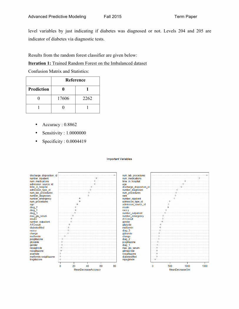
Results from the random forest classifier are given below:
Iteration 1: Trained Random Forest on the Imbalanced dataset
Confusion Matrix and Statistics:
Reference
Prediction 0 1
0 17606 2262
1 0 1
• Accuracy : 0.8862
• Sensitivity : 1.0000000
• Specificity : 0.0004419

Advanced Predictive Modeling Fall 2015 Term Paper
Iteration 2: Trained Random Forest on Balanced dataset with diagnosis variable coded as Yes or
No, as explained earlier
The following plot shows the error rate
The most important variables:

Advanced Predictive Modeling Fall 2015 Term Paper
Confusion Matrix and Statistics:
Reference
Prediction 0 1
0 1678 1166
1 608 1074
• Accuracy : 0.608
• Sensitivity : 0.7340
• Specificity : 0.4795
Predicting the model trained on sampled balanced dataset on the entire data Confusion Matrix and Statistics:
Reference
Prediction 0 1
0 67231 1720
1 20798 9594
• Accuracy : 0.7733
• Sensitivity : 0.7637
• Specificity : 0.8480
Iteration 3: Used association analysis variable for diagnosis instead of diag1, diag2, and diag3 –
slight accuracy improvement
Testing the model on sampled balanced test set
Confusion Matrix and Statistics:
Reference
Prediction 0 1
0 1672 1150
1 614 1090

Advanced Predictive Modeling Fall 2015 Term Paper
• Accuracy : 0.6103
• Sensitivity : 0.7314
• Specificity : 0.4866
Predicting the model trained on sampled balanced dataset on the entire data
Confusion Matrix and Statistics:
Reference
Prediction 0 1
0 66986 1608
1 21043 9706
• Accuracy : 0.772
• Sensitivity : 0.7610
• Specificity : 0.8579
All models were trained on the balanced dataset (except iteration 1) and tested on a balanced test
set. In addition, they were also tested on the entire dataset. The train to test ratio used is 80:20.
Generalized Boosting Models – Gradient Boosted Decision Tree
Another form of ensemble is using gradient boosting to improve upon the accuracy of other
predictive models, generally and for the purpose of this project, decision trees. Gradient boosting
builds the model in a stage-wise fashion combining multiple weak-learners in to a strong learner.
Like many predictive models, parameters can be changed and tested to assist and ensure that the
model is being trained appropriately and not over fitting to the available data. The specific
parameter to be tuned is the number of trees and via cross validation we have determined that the
best number of trees is 500. This results in the lowest Bernoulli deviance. It is also the maximum
number of trees that were tried with this model. Another parameter chosen was the interaction
depth, which is the level of interaction allowed between predictors. When set to two, we are

Advanced Predictive Modeling Fall 2015 Term Paper
fitting a number of decision stumps, therefore to allow versatility and a better fit to the data while
ensuring to dodge the problem of overfitting the dataset, an interaction depth of three was
picked.
One clear advantage of using gradient boosting was the fact that it was not thrown off by our
heavily diverse factor variables of primary, secondary and additional secondary diagnoses.
Where other models failed (for example Random Forest), the only choke for the GBM was
compute time.
Dealing with class imbalance is also a challenge with the gradient boosted model, hence
undersampling of the negative class was performed to ensure that the training set available to the
model was balanced. Accuracy measures were as follows:
• Test set accuracy of the gradient boosted model on the imbalanced dataset (11% incident
rate): 80%
o Unfortunately this is very poor performance as the baseline accuracy we would
expect should be 89%
o Throughout our experience with this dataset however, such results have always
occurred, potentially indicating the lack of predictive power of the available
variables.
• Test set accuracy of the gradient boosted model on the balanced dataset (50% incident
rate): 55%
o This is a marginally better accuracy than randomly assigning outcomes, however
it is clear that the model is doing better when trained with the class imbalance
problem solved.
o Again, feature relevance is probably what is the insight that is being conveyed
through this relatively poor accuracy measure
Using the R package for gradient boosting, relative importance / influence of the available
features was extracted. Shown below is the output.

Advanced Predictive Modeling Fall 2015 Term Paper
Clearly, we can see that the number of in-patient visits is the most relevant to readmission
followed by the primary, additional secondary, and secondary diagnoses. Surprisingly, none of
the medical data related variables are good indicators of readmission according to the GBM. As
discussed earlier, we can chalk this up to our dataset not having the most relevant variables that
predict readmission.
Conclusion
In conclusion, after a lot of data preprocessing, cleaning, and predictive modeling, no one
accuracy score has been better than the baseline accuracy. Logistic regression does an excellent
job, and models that usually deal with high dimensional data well do not stand out such as SVM,
and the ensembles. The poor performance of these classifiers can be attributed to lack of the
underlying predictor for readmission rates. As Professor Ghosh (the instructor of this class)
mentioned, the best predictors of a hospital readmission is not necessarily the medical and
biological data. It usually turns out to be socio-economic indicators at the patient level. The
dataset did not have this information, and we can stipulate that our models would have
performed much better given this information.

Advanced Predictive Modeling Fall 2015 Term Paper
References:
https://onlinecourses.science.psu.edu/stat504/node/149
http://www.ats.ucla.edu/stat/stata/dae/logit.htm
http://web.stanford.edu/~hastie/glmnet/glmnet_alpha.html
http://www.r-bloggers.com/examples-and-resources-on-association-rule-mining-with-r/
http://cran.csiro.au/web/packages/arules/vignettes/arules.pdf
http://www.rdatamining.com/examples/association-rules
https://cran.r-project.org/web/packages/arulesViz/vignettes/arulesViz.pdf
http://chandlerzuo.github.io/blog/2015/03/weightedglm/
http://www.jmlr.org/papers/volume8/owen07a/owen07a.pdf