Lesson 18: Maximum and Minimum Values (Section 041 handout)

Section 4.1Maximum and Minimum Values

V63.0121.041, Calculus I

New York University

November 8, 2010

Announcements

I

Announcements

I

V63.0121.041, Calculus I (NYU) Section 4.1 Maximum and Minimum Values November 8, 2010 2 / 34

Objectives

I Understand and be able toexplain the statement of theExtreme Value Theorem.

I Understand and be able toexplain the statement ofFermat’s Theorem.

I Use the Closed IntervalMethod to find the extremevalues of a function definedon a closed interval.


Notes

Notes

Notes

1

Section 4.1 : Maximum and Minimum ValuesV63.0121.041, Calculus I November 8, 2010

Outline

Introduction

The Extreme Value Theorem

Fermat’s Theorem (not the last one)Tangent: Fermat’s Last Theorem

The Closed Interval Method

Examples


Optimize

Why go to the extremes?

I Rationally speaking, it isadvantageous to find theextreme values of a function(maximize profit, minimizecosts, etc.)

I Many laws of science arederived from minimizingprinciples.

I Maupertuis’ principle:“Action is minimizedthrough the wisdom ofGod.”

Pierre-Louis Maupertuis(1698–1759)V63.0121.041, Calculus I (NYU) Section 4.1 Maximum and Minimum Values November 8, 2010 6 / 34

Notes

Notes

Notes

2


Design

Image credit: Jason TrommV63.0121.041, Calculus I (NYU) Section 4.1 Maximum and Minimum Values November 8, 2010 7 / 34






Optics

Image credit: jacreativeV63.0121.041, Calculus I (NYU) Section 4.1 Maximum and Minimum Values November 8, 2010 9 / 34

Notes

Notes

Notes

3


http://www.flickr.com/photos/trommetter/1338616263/

http://www.flickr.com/photos/jacreative/110448225






Outline

Introduction




Examples


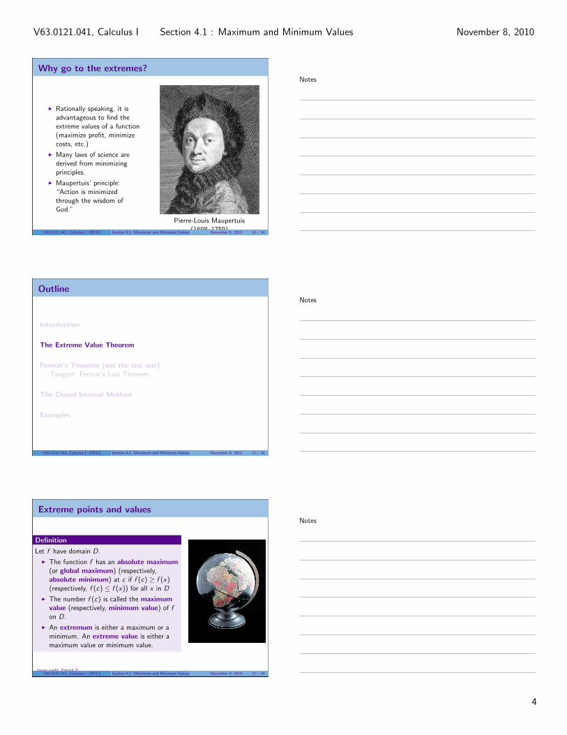
Extreme points and values

Definition

Let f have domain D.

I The function f has an absolute maximum(or global maximum) (respectively,absolute minimum) at c if f (c) ≥ f (x)(respectively, f (c) ≤ f (x)) for all x in D

I The number f (c) is called the maximumvalue (respectively, minimum value) of fon D.

I An extremum is either a maximum or aminimum. An extreme value is either amaximum value or minimum value.

Image credit: Patrick QV63.0121.041, Calculus I (NYU) Section 4.1 Maximum and Minimum Values November 8, 2010 12 / 34

Notes

Notes

Notes

4


http://www.flickr.com/photos/patrick_q/204252734/


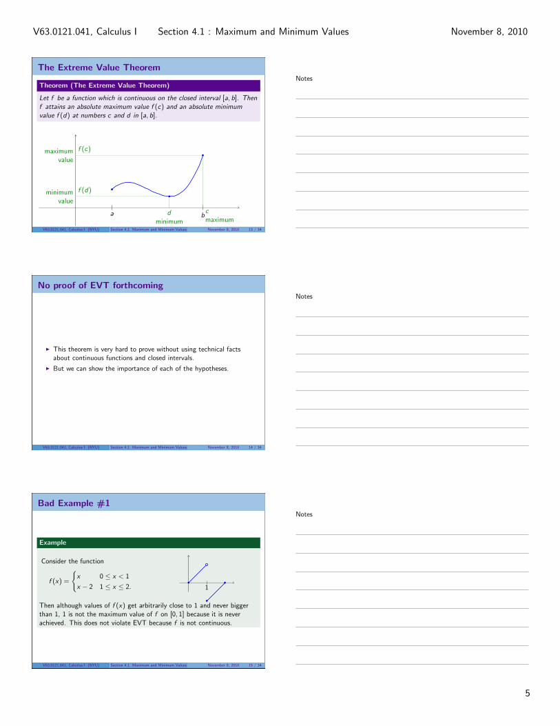
Theorem (The Extreme Value Theorem)

Let f be a function which is continuous on the closed interval [a, b]. Thenf attains an absolute maximum value f (c) and an absolute minimumvalue f (d) at numbers c and d in [a, b].

a bcmaximum

maximumvalue

f (c)

dminimum

minimumvalue

f (d)


No proof of EVT forthcoming

I This theorem is very hard to prove without using technical factsabout continuous functions and closed intervals.

I But we can show the importance of each of the hypotheses.


Bad Example #1

Example

Consider the function

f (x) =

{x 0 ≤ x < 1

x − 2 1 ≤ x ≤ 2.|1

Then although values of f (x) get arbitrarily close to 1 and never biggerthan 1, 1 is not the maximum value of f on [0, 1] because it is neverachieved. This does not violate EVT because f is not continuous.


Notes

Notes

Notes

5


Bad Example #2

Example

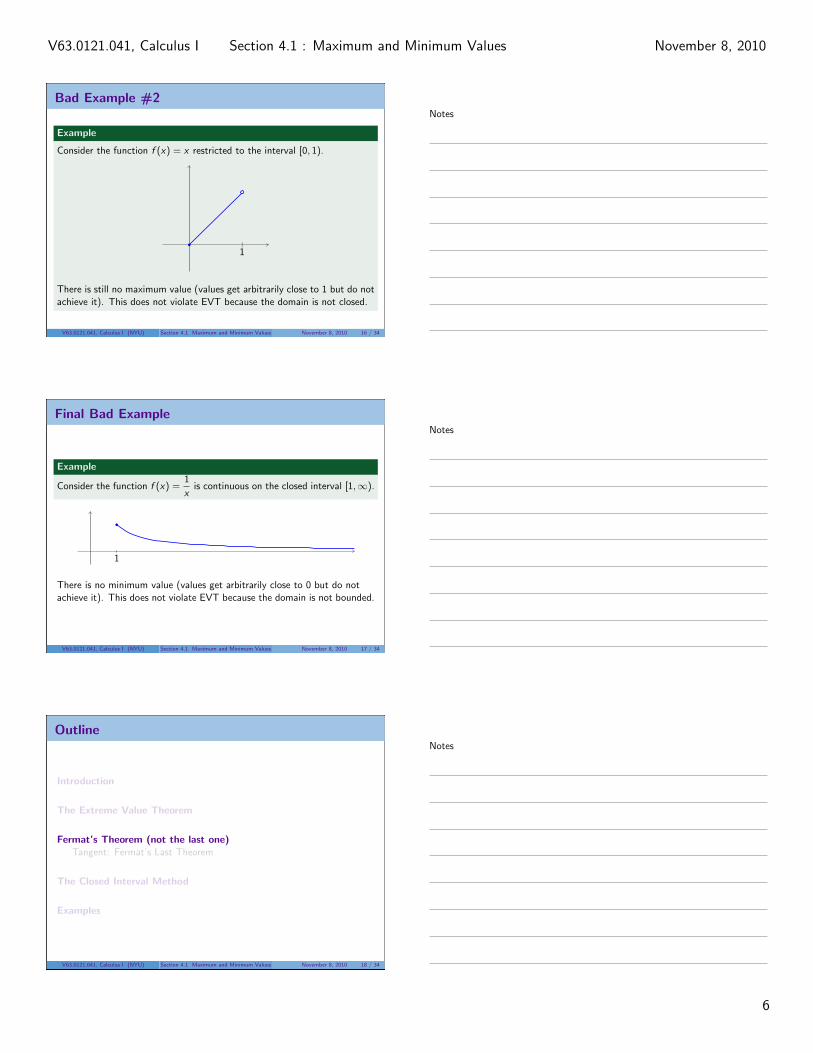
Consider the function f (x) = x restricted to the interval [0, 1).

|1

There is still no maximum value (values get arbitrarily close to 1 but do notachieve it). This does not violate EVT because the domain is not closed.


Final Bad Example

Example

Consider the function f (x) =1

xis continuous on the closed interval [1,∞).

1

There is no minimum value (values get arbitrarily close to 0 but do notachieve it). This does not violate EVT because the domain is not bounded.


Outline

Introduction




Examples


Notes

Notes

Notes

6


Local extrema

Definition

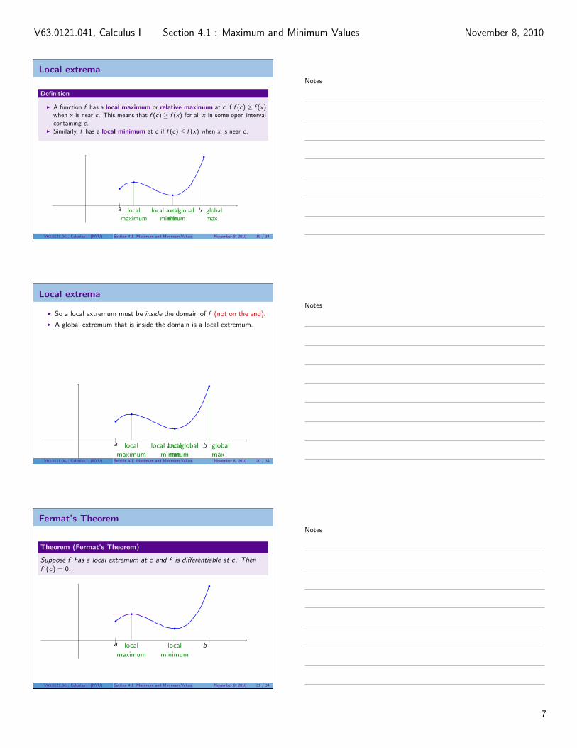
I A function f has a local maximum or relative maximum at c if f (c) ≥ f (x)when x is near c. This means that f (c) ≥ f (x) for all x in some open intervalcontaining c .

I Similarly, f has a local minimum at c if f (c) ≤ f (x) when x is near c .

|a

|blocal

maximumlocal

minimumglobalmax

local and globalmin


Local extrema

I So a local extremum must be inside the domain of f (not on the end).

I A global extremum that is inside the domain is a local extremum.

|a

|blocal

maximumlocal

minimumglobalmax

local and globalmin


Fermat’s Theorem

Theorem (Fermat’s Theorem)

Suppose f has a local extremum at c and f is differentiable at c. Thenf ′(c) = 0.

|a

|blocal

maximumlocal

minimum


Notes

Notes

Notes

7


Sketch of proof of Fermat’s Theorem

Suppose that f has a local maximum at c .

I If x is slightly greater than c , f (x) ≤ f (c). This means

f (x)− f (c)

x − c≤ 0 =⇒ lim

x→c+

f (x)− f (c)

x − c≤ 0

I The same will be true on the other end: if x is slightly less than c,f (x) ≤ f (c). This means

f (x)− f (c)

x − c≥ 0 =⇒ lim

x→c−

f (x)− f (c)

x − c≥ 0

I Since the limit f ′(c) = limx→c

f (x)− f (c)

x − cexists, it must be 0.


Meet the Mathematician: Pierre de Fermat

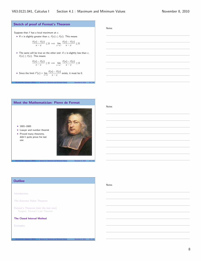
I 1601–1665

I Lawyer and number theorist

I Proved many theorems,didn’t quite prove his lastone


Outline

Introduction




Examples


Notes

Notes

Notes

8


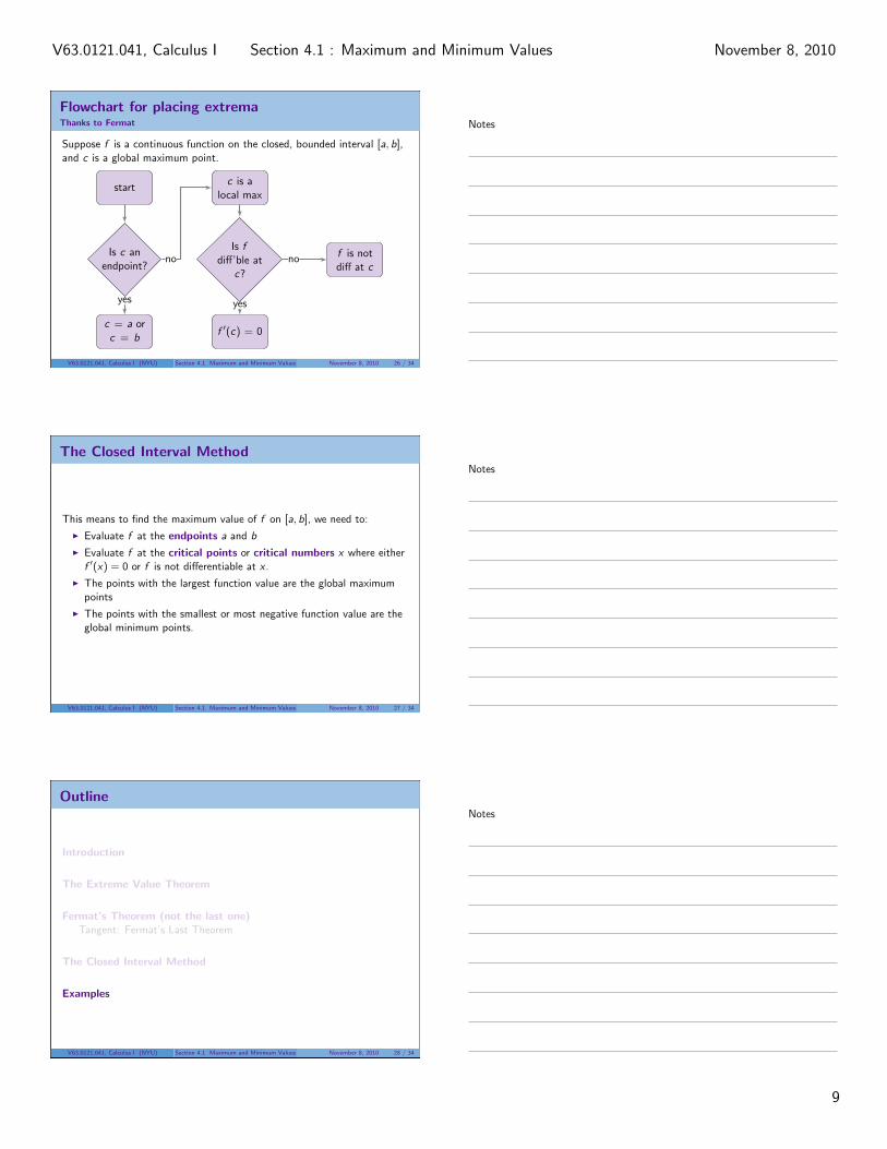
Flowchart for placing extremaThanks to Fermat

Suppose f is a continuous function on the closed, bounded interval [a, b],and c is a global maximum point.

start

Is c anendpoint?

c = a orc = b

c is alocal max

Is fdiff’ble at

c?

f is notdiff at c

f ′(c) = 0

no

yes

no

yes



This means to find the maximum value of f on [a, b], we need to:

I Evaluate f at the endpoints a and b

I Evaluate f at the critical points or critical numbers x where eitherf ′(x) = 0 or f is not differentiable at x .

I The points with the largest function value are the global maximumpoints

I The points with the smallest or most negative function value are theglobal minimum points.


Outline

Introduction




Examples


Notes

Notes

Notes

9


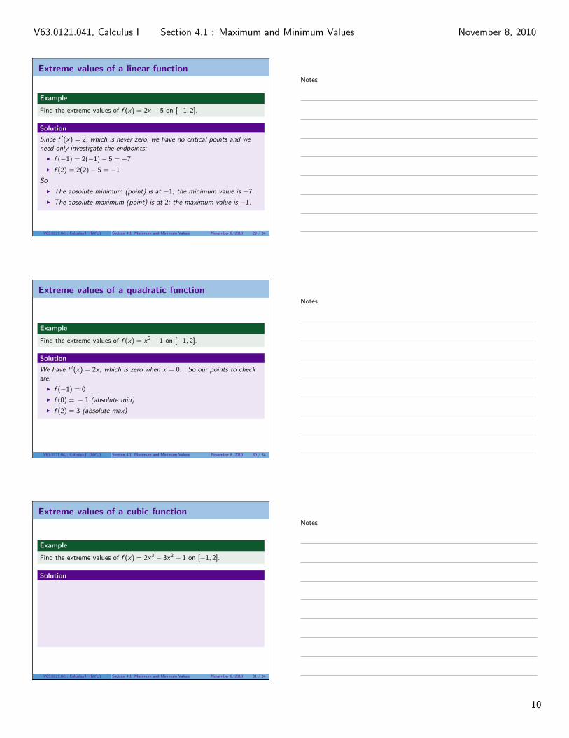
Extreme values of a linear function

Example

Find the extreme values of f (x) = 2x − 5 on [−1, 2].

Solution

Since f ′(x) = 2, which is never zero, we have no critical points and weneed only investigate the endpoints:

I f (−1) = 2(−1)− 5 = −7

I f (2) = 2(2)− 5 = −1

So

I The absolute minimum (point) is at −1; the minimum value is −7.

I The absolute maximum (point) is at 2; the maximum value is −1.


Extreme values of a quadratic function

Example

Find the extreme values of f (x) = x2 − 1 on [−1, 2].

Solution

We have f ′(x) = 2x, which is zero when x = 0. So our points to checkare:

I f (−1) = 0

I f (0) = − 1 (absolute min)

I f (2) = 3 (absolute max)


Extreme values of a cubic function

Example

Find the extreme values of f (x) = 2x3 − 3x2 + 1 on [−1, 2].

Solution

Since f ′(x) = 6x2 − 6x = 6x(x − 1), we have critical points at x = 0 andx = 1. The values to check are

I f (−1) = − 4 (global min)

I f (0) = 1 (local max)

I f (1) = 0 (local min)

I f (2) = 5 (global max)


Notes

Notes

Notes

10


Extreme values of an algebraic function

Example

Find the extreme values of f (x) = x2/3(x + 2) on [−1, 2].

Solution

Write f (x) = x5/3 + 2x2/3, then

f ′(x) =5

3x2/3 +

4

3x−1/3 =

1

3x−1/3(5x + 4)

Thus f ′(−4/5) = 0 and f is not differentiable at 0. So our points to checkare:

I f (−1) = 1

I f (−4/5) = 1.0341 (relative max)

I f (0) = 0 (absolute min)

I f (2) = 6.3496 (absolute max)


Extreme values of another algebraic function

Example

Find the extreme values of f (x) =√

4− x2 on [−2, 1].

Solution

We have f ′(x) = − x√4− x2

, which is zero when x = 0. (f is not

differentiable at ±2 as well.) So our points to check are:

I f (−2) = 0 (absolute min)

I f (0) = 2 (absolute max)

I f (1) =√

3


Summary

I The Extreme Value Theorem: a continuous function on a closedinterval must achieve its max and min

I Fermat’s Theorem: local extrema are critical points

I The Closed Interval Method: an algorithm for finding global extrema

I Show your work unless you want to end up like Fermat!


Notes

Notes

Notes

11


Technology

Lesson 18: Maximum and Minimum Values (Section 041 handout)