Observed glacier and volatile distribution on Pluto from atmosphere–topography processes

0 0 M O N T H 2 0 1 6 | V O L 0 0 0 | N A T U R E | 1

LETTERdoi:10.1038/nature19337

Observed glacier and volatile distribution on Pluto from atmosphere–topography processesTanguy Bertrand1 & François Forget1

Pluto has a variety of surface frosts and landforms as well as a complex atmosphere1. There is ongoing geological activity related to the massive Sputnik Planum glacier, mostly made of nitrogen (N2) ice mixed with solid carbon monoxide and methane2, covering the 4-kilometre-deep, 1,000-kilometre-wide basin of Sputnik Planum1,3 near the anti-Charon point. The glacier has been suggested to arise from a source region connected to the deep interior, or from a sink collecting the volatiles released planetwide1. Thin deposits of N2 frost, however, were also detected at mid-northern latitudes and methane ice was observed to cover most of Pluto except for the darker, frost-free equatorial regions2. Here we report numerical simulations of the evolution of N2, methane and carbon monoxide on Pluto over thousands of years. The model predicts N2 ice accumulation in the deepest low-latitude basin and the threefold increase in atmospheric pressure that has been observed to occur since 19884–6. This points to atmospheric–topographic processes as the origin of Sputnik Planum’s N2 glacier. The same simulations also reproduce the observed quantities of volatiles in the atmosphere and show frosts of methane, and sometimes N2, that seasonally cover the mid- and high latitudes, explaining the bright northern polar cap reported in the 1990s7,8 and the observed ice distribution in 20152. The model also predicts that most of these seasonal frosts should disappear in the next decade.

To understand the distribution of volatiles on Pluto, we developed a numerical volatile transport model designed to represent the physical processes that control their condensation, sublimation and atmospheric transport forced by the variation of insolation throughout multiple annual cycles (see Methods). The model derives from a full Pluto General Circulation Model9 (GCM) able to calculate the three- dimensional transport and mixing in the atmosphere, but too slow to run for multiple Pluto seasons. To simulate the cycles of the volatiles for thousands of terrestrial years in a practical amount of computing time, atmospheric dynamics and transport were parameterized using a simplified redistribution of N2, carbon monoxide (CO) and methane (CH4) gases with characteristic timescales estimated from ‘short’ GCM simulations. We start our simulations with Pluto uniformly covered with 50 kg m−2 of each kind of ice, and let the modelled planet evolve for 50,000 terrestrial years. The seasonal ice cycles are then repeatable from one Pluto year to the next. However, they strongly depend on key model parameters such as the topography, the albedo and the emissivity of the ices (only partly constrained by observation and theory), the total ice inventories, and the thermal conductivity of the shallow (centimetres) and deep (metres) subsurface, which control the diurnal10 and seasonal global thermal inertia, respectively.

Assuming a flat surface, the model reproduces the results of pre-New Horizons N2 cycle models11,12. Like those models, we find that

1Laboratoire de Météorologie Dynamique, IPSL, Sorbonne Universités, UPMC Université Paris 06, CNRS, BP99, 4 place Jussieu, 75005 Paris, France.

Ice-free

N2 + CH4 + CO

Pure CH4

Initial distribution

N2, CH4, COices everywhere

After 250 years After 4,000 years

All N2 ice trappedin the basin

After 10,000 years

1994Ls = 15°

2002Ls = 34°

2015Ls = 63°

2030Ls = 91°

After about 50,000 years

‘Sputnik Planum’-likebasin (3 km deep)

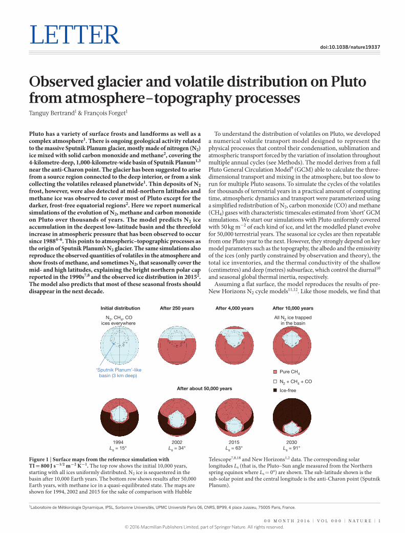
Figure 1 | Surface maps from the reference simulation with TI = 800 J s−1/2 m−2 K−1. The top row shows the initial 10,000 years, starting with all ices uniformly distributed. N2 ice is sequestered in the basin after 10,000 Earth years. The bottom row shows results after 50,000 Earth years, with methane ice in a quasi-equilibrated state. The maps are shown for 1994, 2002 and 2015 for the sake of comparison with Hubble

Telescope7,8,18 and New Horizons1,2 data. The corresponding solar longitudes Ls (that is, the Pluto–Sun angle measured from the Northern spring equinox where Ls = 0°) are shown. The sub-latitude shown is the sub-solar point and the central longitude is the anti-Charon point (Sputnik Planum).

© 2016 Macmillan Publishers Limited, part of Springer Nature. All rights reserved.

http://www.nature.com/doifinder/10.1038/nature19337

2 | N A T U R E | V O L 0 0 0 | 0 0 M O N T H 2 0 1 6

LETTERRESEARCH

seasonal thermal inertia (TI, measured in units of J s−1/2 m−2 K−1), a poorly known parameter, is the key driver of the N2 cycle. On a flat Pluto, two end- member behaviours arise. High TI leads to the formation of a permanent band of N2 ice in the equatorial regions because the annual-mean insolation is lower there than at the poles, as a result of the high obliquity of Pluto13. On the other hand, low TI yields more pronounced seasonal variations and the formation of N2 seasonal polar caps only.

We examined the effect of topography, whose origin on Pluto we do not discussed here, by placing a 4-km-deep circular crater at the location of Sputnik Planum and two smaller craters corresponding to the informally called Burney (1,000 m deep) and Guest (800 m deep) craters1.

With such an orography, in the high-TI cases, all the N2 ice is entirely sequestered in the modelled ‘Sputnik Planum’-like basin after roughly 10,000 Earth years (Fig. 1). The N2 ice does not form a permanent latitudinal band, as in the flat planet case, because the basin induces a higher surface pressure and thus a higher condensation temperature, which leads to a stronger thermal infrared cooling and a higher condensation rate. This phenomenon is also observed on Mars, where CO2 frosts preferably form at low elevations such as the Hellas basin14 (Extended Data Fig. 1). The characteristics of Sputnik Planum are thus

explained by its latitude and depth rather than by a connection with putative N2 reservoirs in the deep interior.

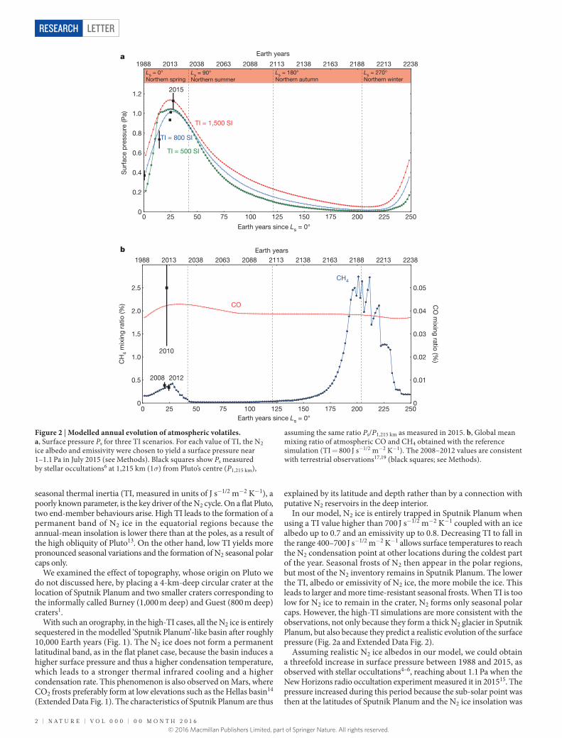
In our model, N2 ice is entirely trapped in Sputnik Planum when using a TI value higher than 700 J s−1/2 m−2 K−1 coupled with an ice albedo up to 0.7 and an emissivity up to 0.8. Decreasing TI to fall in the range 400–700 J s−1/2 m−2 K−1 allows surface temperatures to reach the N2 condensation point at other locations during the coldest part of the year. Seasonal frosts of N2 then appear in the polar regions, but most of the N2 inventory remains in Sputnik Planum. The lower the TI, albedo or emissivity of N2 ice, the more mobile the ice. This leads to larger and more time-resistant seasonal frosts. When TI is too low for N2 ice to remain in the crater, N2 forms only seasonal polar caps. However, the high-TI simulations are more consistent with the observations, not only because they form a thick N2 glacier in Sputnik Planum, but also because they predict a realistic evolution of the surface pressure (Fig. 2a and Extended Data Fig. 2).

Assuming realistic N2 ice albedos in our model, we could obtain a threefold increase in surface pressure between 1988 and 2015, as observed with stellar occultations4–6, reaching about 1.1 Pa when the New Horizons radio occultation experiment measured it in 201515. The pressure increased during this period because the sub-solar point was then at the latitudes of Sputnik Planum and the N2 ice insolation was

0 25 50 75 100 125 150 175 200 225 250

Earth years since Ls = 0°

Earth years since Ls = 0°

0

0.2

0.4

0.6

0.8

1.0

1.2

Sur

face

pre

ssur

e (P

a)

2015

Ls = 0° Northern spring

Ls = 90°Northern summer

Ls = 180°Northern autumn

Ls = 270° Northern winter

TI = 500 SI

TI = 800 SI

TI = 1,500 SI

1988 2013 2038 2063 2088 2113 2138 2163 2188 2213 2238

Earth years

0 25 50 75 100 125 150 175 200 225 2500

0.5

1.0

1.5

2.0

2.5

CH

4 m

ixin

g ra

tio (%

)

2008 2012

CH4

CO

0

0.01

0.02

0.03

0.04

0.05

CO

mixing ratio (%

)

2010

1988 2013 2038 2063 2088 2113 2138 2163 2188 2213 2238Earth years

a

b

Figure 2 | Modelled annual evolution of atmospheric volatiles. a, Surface pressure Ps for three TI scenarios. For each value of TI, the N2 ice albedo and emissivity were chosen to yield a surface pressure near 1–1.1 Pa in July 2015 (see Methods). Black squares show Ps measured by stellar occultations6 at 1,215 km (1σ) from Pluto’s centre (P1,215 km),

assuming the same ratio Ps/P1,215 km as measured in 2015. b, Global mean mixing ratio of atmospheric CO and CH4 obtained with the reference simulation (TI = 800 J s−1/2 m−2 K−1). The 2008–2012 values are consistent with terrestrial observations17,19 (black squares; see Methods).


0 0 M O N T H 2 0 1 6 | V O L 0 0 0 | N A T U R E | 3

LETTER RESEARCH

near maximum. After 2015, the modelled mean pressure decreased because the insolation in Sputnik Planum was reduced, initially because the subsolar point was at higher latitudes and later because Pluto moved away from the Sun.

The stellar occultation pressure observations provide quantitative constraints for models. If we tune the N2 ice albedo to obtain surface pressure in the 1–1.2 Pa range in 2015 as observed (Fig. 2), we find that low TI leads to a stronger increase of surface pressures in 1988–2015. In our simulations, the ratio of surface pressure Ps in 2015 to that in 1988—that is, Ps(2015)/Ps(1988)—is near 2.5, 3, 4.5 and 6 for TI values of 1,000 J s−1/2 m−2 K−1, 800 J s−1/2 m−2 K−1, 600 J s−1/2 m−2 K−1 and 400 J s−1/2 m−2 K−1 respectively. TI values lower than 500 J s−1/2 m−2 K−1 are thus ruled out. The higher values of TI are sufficient to maintain a substantial surface pressure of several millipascals throughout Pluto’s orbit (Fig. 2).

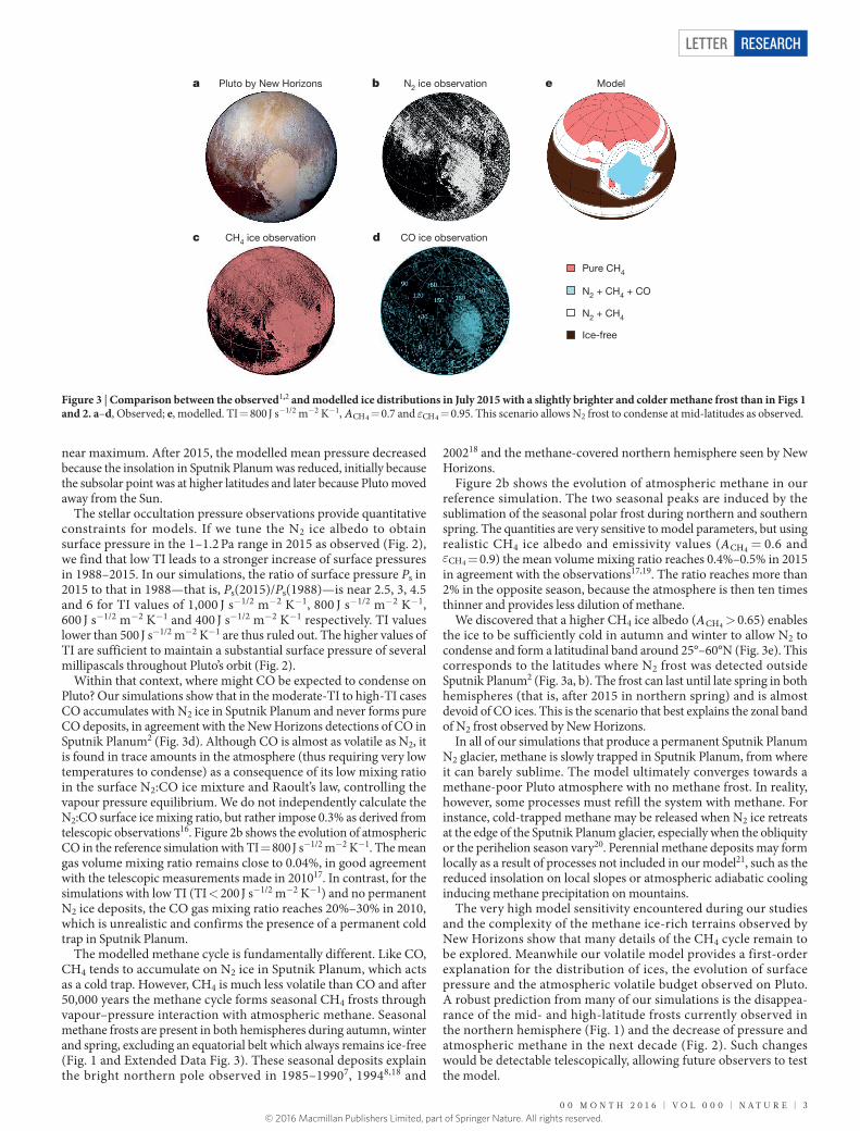
Within that context, where might CO be expected to condense on Pluto? Our simulations show that in the moderate-TI to high-TI cases CO accumulates with N2 ice in Sputnik Planum and never forms pure CO deposits, in agreement with the New Horizons detections of CO in Sputnik Planum2 (Fig. 3d). Although CO is almost as volatile as N2, it is found in trace amounts in the atmosphere (thus requiring very low temperatures to condense) as a consequence of its low mixing ratio in the surface N2:CO ice mixture and Raoult’s law, controlling the vapour pressure equilibrium. We do not independently calculate the N2:CO surface ice mixing ratio, but rather impose 0.3% as derived from telescopic observations16. Figure 2b shows the evolution of atmospheric CO in the reference simulation with TI = 800 J s−1/2 m−2 K−1. The mean gas volume mixing ratio remains close to 0.04%, in good agreement with the telescopic measurements made in 201017. In contrast, for the simulations with low TI (TI < 200 J s−1/2 m−2 K−1) and no permanent N2 ice deposits, the CO gas mixing ratio reaches 20%–30% in 2010, which is unrealistic and confirms the presence of a permanent cold trap in Sputnik Planum.

The modelled methane cycle is fundamentally different. Like CO, CH4 tends to accumulate on N2 ice in Sputnik Planum, which acts as a cold trap. However, CH4 is much less volatile than CO and after 50,000 years the methane cycle forms seasonal CH4 frosts through vapour–pressure interaction with atmospheric methane. Seasonal methane frosts are present in both hemispheres during autumn, winter and spring, excluding an equatorial belt which always remains ice-free (Fig. 1 and Extended Data Fig. 3). These seasonal deposits explain the bright northern pole observed in 1985–19907, 19948,18 and

200218 and the methane-covered northern hemisphere seen by New Horizons.

Figure 2b shows the evolution of atmospheric methane in our reference simulation. The two seasonal peaks are induced by the sublimation of the seasonal polar frost during northern and southern spring. The quantities are very sensitive to model parameters, but using realistic CH4 ice albedo and emissivity values (ACH4 = 0.6 and εCH4 = 0.9) the mean volume mixing ratio reaches 0.4%–0.5% in 2015 in agreement with the observations17,19. The ratio reaches more than 2% in the opposite season, because the atmosphere is then ten times thinner and provides less dilution of methane.

We discovered that a higher CH4 ice albedo (ACH4 > 0.65) enables the ice to be sufficiently cold in autumn and winter to allow N2 to condense and form a latitudinal band around 25°–60°N (Fig. 3e). This corresponds to the latitudes where N2 frost was detected outside Sputnik Planum2 (Fig. 3a, b). The frost can last until late spring in both hemispheres (that is, after 2015 in northern spring) and is almost devoid of CO ices. This is the scenario that best explains the zonal band of N2 frost observed by New Horizons.

In all of our simulations that produce a permanent Sputnik Planum N2 glacier, methane is slowly trapped in Sputnik Planum, from where it can barely sublime. The model ultimately converges towards a methane-poor Pluto atmosphere with no methane frost. In reality, however, some processes must refill the system with methane. For instance, cold-trapped methane may be released when N2 ice retreats at the edge of the Sputnik Planum glacier, especially when the obliquity or the perihelion season vary20. Perennial methane deposits may form locally as a result of processes not included in our model21, such as the reduced insolation on local slopes or atmospheric adiabatic cooling inducing methane precipitation on mountains.

The very high model sensitivity encountered during our studies and the complexity of the methane ice-rich terrains observed by New Horizons show that many details of the CH4 cycle remain to be explored. Meanwhile our volatile model provides a first- order explanation for the distribution of ices, the evolution of surface pressure and the atmospheric volatile budget observed on Pluto. A robust prediction from many of our simulations is the disappea-rance of the mid- and high-latitude frosts currently observed in the northern hemisphere (Fig. 1) and the decrease of pressure and atmospheric methane in the next decade (Fig. 2). Such changes would be detectable telescopically, allowing future observers to test the model.

b N2 ice observation

c CH4 ice observation

e Model

d CO ice observation

Pure CH4

Ice-free

N2 + CH4 + CO

N2 + CH4

a Pluto by New Horizons

Figure 3 | Comparison between the observed1,2 and modelled ice distributions in July 2015 with a slightly brighter and colder methane frost than in Figs 1 and 2. a–d, Observed; e, modelled. TI = 800 J s−1/2 m−2 K−1, ACH4 = 0.7 and εCH4 = 0.95. This scenario allows N2 frost to condense at mid-latitudes as observed.


4 | N A T U R E | V O L 0 0 0 | 0 0 M O N T H 2 0 1 6

LETTERRESEARCH

Online Content Methods, along with any additional Extended Data display items and Source Data, are available in the online version of the paper; references unique to these sections appear only in the online paper.

Received 1 June; accepted 19 July 2016.

Published online 19 September 2016.

1. Stern, A. S. et al. The Pluto system: initial results from its exploration by New Horizons. Science 350, aad1815 (2015).

2. Grundy, W. M. et al. Surface compositions across Pluto and Charon. Science 351, aad9189 (2016).

3. Moore, J. F. et al. The geology of Pluto and Charon through the eyes of New Horizons. Science 351, 1284–1293 (2016).

4. Elliot, J. L. et al. Changes in Pluto’s atmosphere: 1988–2006. Astrophys. J. 134, 1–13 (2007).

5. Olkin, C. B. et al. Evidence that Pluto’s atmosphere does not collapse from occultations including the 2013 May 04 event. Icarus 246, 220–225 (2015).

6. Sicardy, B. et al. Pluto’s atmosphere from the 29 June 2015 ground-based stellar occultation at the time of the New Horizons flyby. Astrophys. J. Lett. 819, L38 (2016).

7. Buie, M. W., Tholen, D. J. & Horne, K. Albedo maps of Pluto and Charon—initial mutual event results. Icarus 97, 211–227 (1992).

8. Stern, S. A., Buie, M. W. & Trafton, L. M. HST high-resolution images and maps of Pluto. Astron. J. 113, 827–843 (1997).

9. Forget, F., Bertrand, T., Vangvichith, M. & Leconte, A. 3D global climate model of the Pluto atmosphere to interpret New Horizons observations, including the N2, CH4 and CO cycles and the formation of organic hazes. Abstract DPS 47, 105.12, http://adsabs.harvard.edu/abs/2015DPS....4710512F (2015).

10. Lellouch, E., Stansberry, J., Emery, J., Grundy, W. & Cruikshank, D. Thermal properties of Pluto’s and Charon’s surfaces from Spitzer observations. Icarus 214, 701–716 (2011).

11. Hansen, C. J. & Paige, D. A. Seasonal nitrogen cycles on Pluto. Icarus 120, 247–265 (1996).

12. Young, L. A. Pluto’s seasons: new predictions for New Horizons. Astrophys. J. 766, L22 (2013).

Acknowledgements We thank the New Horizons team for this successful mission. We also thank E. Lellouch, E. Millour and M. J. Wolff for comments on the manuscript. We are grateful to M. Vangvichith for her contribution to an early version of the model, and to the Institut de Formation Doctorale for supporting this work.

Author Contributions F.F. and T.B. designed and developed the model. T.B. performed the simulations. Both authors contributed to the writing of the manuscript.

Author Information Reprints and permissions information is available at www.nature.com/reprints. The authors declare no competing financial interests. Readers are welcome to comment on the online version of the paper. Correspondence and requests for materials should be addressed to F.F. ([email protected]).

13. Hamilton, D. P. et al. The cold and icy heart of Pluto. Abstract AGU 48, P51, 2036, https://agu.confex.com/agu/fm15/meetingapp.cgi/Paper/75719 (2015).

14. James, P. B., Kieffer, H. H. & Paige, D. A. in Mars (eds Kieffer, H., Jakosky, B., Snyder C. & Matthews, M.) 934–968 (Univ. Arizona Press, 1992).

15. Gladstone, G. R. et al. The atmosphere of Pluto as observed by New Horizons. Science 351, aad8866 (2016).

16. Merlin, F. New constraints on the surface of Pluto. Astron. Astrophys. 582, A39 (2015).

17. Lellouch, E., de Bergh, C., Sicardy, B., Kaufl, H. U. & Smette, A. High resolution spectroscopy of Pluto’s atmosphere: detection of the 2.3 μ m CH4 bands and evidence for carbon monoxide. Astron. Astrophys. 530, L4 (2011).

18. Buie, M. W., Grundy, W. M., Young, E. F., Young, L. A. & Stern, S. A. Pluto and Charon with the Hubble Space Telescope. II. Resolving changes on Pluto’s surface and a map for Charon. Astron. J. 139, 1128–1143 (2010).

19. Lellouch, E. et al. Exploring the spatial, temporal, and vertical distribution of methane in Pluto’s atmosphere. Icarus 246, 268–278 (2015).

20. Earle, A. M. & Binzel, R. P. Pluto’s insolation history: latitudinal variations and effects on atmospheric pressure. Icarus 250, 405–412 (2015).

21. Stansberry, J. A. et al. A model for the overabundance of methane in the atmospheres of Pluto and Triton. Planet. Space Sci. 44, 1051–1063 (1996).



http://adsabs.harvard.edu/abs/2015DPS....4710512F

http://www.nature.com/reprints


mailto:[email protected]

https://agu.confex.com/agu/fm15/meetingapp.cgi/Paper/75719

LETTER RESEARCH

22. Fray, N. & Schmitt, B. Sublimation of ices of astrophysical interest: a bibliographic review. Planet. Space Sci. 57, 2053–2080 (2009).

23. Forget, F. et al. A post-New Horizons global climate model of Pluto including the N2, CH4 and CO cycles. Icarus (submitted).

METHODSPluto’s surface is represented by a grid of 32 longitudes × 24 latitudes. At each point the model computes the surface radiative budget, the exchange of heat with the subsurface by conduction, and the exchanges of volatile (N2, CO, CH4) with the atmosphere.Insolation and radiative cooling. At each time step the local solar insolation is calculated taking into account the variation of the Pluto–Sun distance throughout its orbit, the seasonal inclination and the diurnal cycle. The atmosphere is assumed to be transparent at all wavelengths.Thermal conduction into the subsurface. The heat flux from and to the subsurface is computed using a classical heat conduction model with thermal inertia I as the key parameter controlling the influence of the subsurface heat storage and conduction on the surface temperature: I = λC , with λ the heat conductivity of the ground (in units of J s−1 m−1 K−1) and C the ground volumetric specific heat (J m−3 K−1). In practice, we thus use I as the key model parameter, assuming a constant value for C = 106 J m−3 K−1 and making λ vary accordingly. On Pluto one needs to simultaneously capture (1) the short-period diurnal thermal waves in the near-surface, low-TI terrain and (2) the much longer seasonal thermal waves which can penetrate deep in the high-TI substrate. The diurnal thermal inertia is set to 20 J s−1/2 m−2 K−1, as inferred from Spitzer thermal observations10, and the seasonal TI is varied in the range 200–2,000 J s−1/2 m−2 K−1, as discussed in the main text.

The modelled diurnal and annual skin depths are 0.008 m and 10–100 m respectively. To adequately resolve these scale lengths, the subsurface is divided into 22 discrete layers, with a geometrically stretched distribution of layers with higher resolution near the surface (the depth of the first layer is 1.4 × 10−4 m) and a coarser grid for deeper layers (the deepest layer depth is near 300 m). Our simulations are performed assuming no internal heat flux.Volatile condensation and sublimation. We computed the phase changes of N2, CH4 and CO using the thermodynamic relations from ref. 22, taking into account the α - and β -phase transitions. The rate of N2 condensation or sublimation is derived from the amount of latent heat required to keep temperatures at the frost point if N2 ice is present. CH4 and CO are minor constituents and their exchange with the atmosphere depends on the turbulent fluxes given by:

ρ= −F C U q q( ) (1)d surf

with qsurf the saturation vapour pressure mass mixing ratio (in kg kg−1) at the considered surface temperature, q the mass mixing ratio in the atmosphere, ρ the air density, U the horizontal wind velocity at z1 = 5 m above the surface (0.5 m s−1), and Cd the drag coefficient at 5 m above the local surface set to 0.06.

Since the ices may form solid solutions, to compute qsurf when N2 ice is present we applied Raoult’s law considering the mixtures N2:CH4 and N2:CO with 0.5% of methane and 0.3% of CO respectively, as retrieved from telescopic observations16.

The modelled volatile cycles are slightly affected by the limited grid resolution. For instance, in Fig. 2b the ‘saw-tooth’ variations around Ls = 200° are artefacts resulting from the sudden sublimation of latitudinal bands of methane ice on the low-resolution grid.Atmospheric horizontal ‘transport’ and effect of topography. To represent horizontal transport after surface exchanges, atmospheric species are mixed with an adjustable intensity, taking into account the effect of topography. For N2, at each time step the surface pressure ps at altitude z is forced towards the global mean value by integrating the following equation:

τ∂∂=−

−

− /

− /

pt

p p1 ee

(2)z H

z Hs

Ns s

2

with H the near-surface scale height (about 18 km), < > the planetary average operator, and τN2 the characteristic mixing timescale (in seconds). Similarly, for a trace species like CH4, the local mass mixing ratio q mixing is given by:

τ∂∂=−

−

qt

qqpp

1 (3)CH

s

s4

On the basis of tests performed with the Pluto General Circulation Model9 (see below), we set τCH4 = 107 s (about four terrestrial months), and τN2 = 1 s (instantaneous mixing). Note that adiabatic cooling inducing atmospheric condensation is not taken into account.Glacier flow modelling. In the modelled Sputnik Planum basin, N2 tends to condense first where there is N2 ice, essentially because the albedo difference between the ice and the substrate favours further condensation on the ice. Consequently, the ice tends to accumulate in only a fraction of the basin. In reality, massive N2 ice deposits should flow like terrestrial glaciers3. This can affect the evolution of surface pressure, since a smaller surface of N2 ice will be available for condensation and sublimation. To address this issue, we model the flow of N2 ice in the basin by redistributing it locally from a point with a large amount of ice to the nearest-neighbour points with less ice. We use a characteristic speed of 7 cm per Pluto day (about 1 cm per terrestrial day), which allows the crater to be filled with ice after two Pluto years.The three-dimensional GCM used to tune the volatile transport model. The full three-dimensional GCM9 will be described in detail elsewhere23. It is a three- dimensional atmospheric model which uses the same horizontal grid as does the two-dimensional volatile transport model used here, but with 25 layers in the vertical (starting at height 7 m, and reaching 250 km, with most of the levels in the first 15 km in order to obtain a good resolution close to the surface). In addition to the subsurface thermal conduction and surface volatile condensation and sublimation processes already used in the volatile-transport model described above, the following features are included:(1) A finite difference three-dimensional dynamical core to solve the primitive equation of meteorology.(2) A three-dimensional transport scheme to transport atmospheric species like CO gas and CH4 gas and ice.(3) In the atmosphere, radiative heating and cooling is taken into account by computing the amount of CH4 molecules, and cooling by the thermal infrared rotational lines of CO is taken into account by assuming a constant mixing ratio of 0.05%.(4) Turbulent mixing and convection in the boundary layer.(5) Atmospheric molecular thermal conduction and viscosity.(6) Atmospheric CH4 condensation and transport of CH4 ice cloud particles.Design of the reference simulations and comparison with observations. The simulations shown in Fig. 2a have been performed using an N2 ice emissivity of 0.8 and different N2 ice albedo chosen to yield realistic pressure in 2015: AN2 = 0.73 for TI = 500 J s−1/2 m−2 K−1; AN2 = 0.71 for TI = 800 J s−1/2 m−2 K−1; AN2 = 0.69 for TI = 1,500 J s−1/2 m−2 K−1.

The observed CH4 mixing ratios shown in Fig. 2b (error bars) are in the range 0.38 ± 0.06% (for 2008) and 0.34 ± 0.06% (for 2012)19 (E. Lellouch, personal communication), and CO mixing ratios are in the range . − .

+ .0 05 0 0250 1 % (for 2010)17

with 2σ error bars. The central values of the CH4 mixing ratios are computed from the weighted average of the values obtained from the different simulations in Lellouch et al.19, by their own uncertainty. The error bar takes into account the dispersion between the central values and the noise uncertainty.Code availability. All model versions are freely available upon request by contacting F.F. ([email protected]).


LETTERRESEARCH

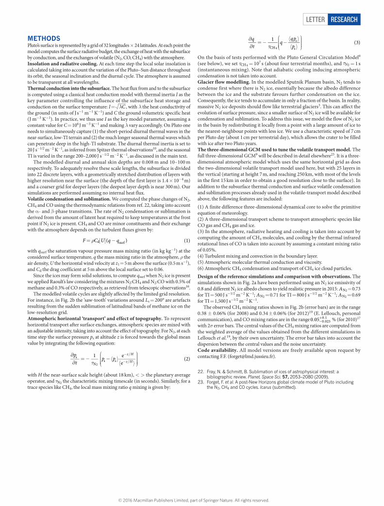
Extended Data Figure 1 | Mars in mid-southern spring. This composite image shows the 7-km-deep, 2,000-km-wide deep Hellas Planitia impact basin covered by seasonal CO2 ice. The physical processes that favour the condensation of the CO2 atmosphere at the bottom of the Hellas basin is the same as for Pluto’s N2 atmosphere in Sputnik Planum. In both basins, surface pressures are larger than in the surrounding regions and condensation temperatures Tc are higher. This corresponds to a stronger

thermal infrared cooling (proportional to Tc4), which is balanced by

a proportionally more intense condensation rate (latent heat). Images obtained by the Mars Global Surveyor Mars Orbiter Camera in November 2006, at solar longitude (the Mars–Sun angle, measured from the Northern Hemisphere spring equinox where Ls = 0°) Ls = 137° (image credit NASA/JPL/MSSS; http://photojournal.jpl.nasa.gov/catalog/PIA01888).


http://photojournal.jpl.nasa.gov/catalog/PIA01888

LETTER RESEARCH

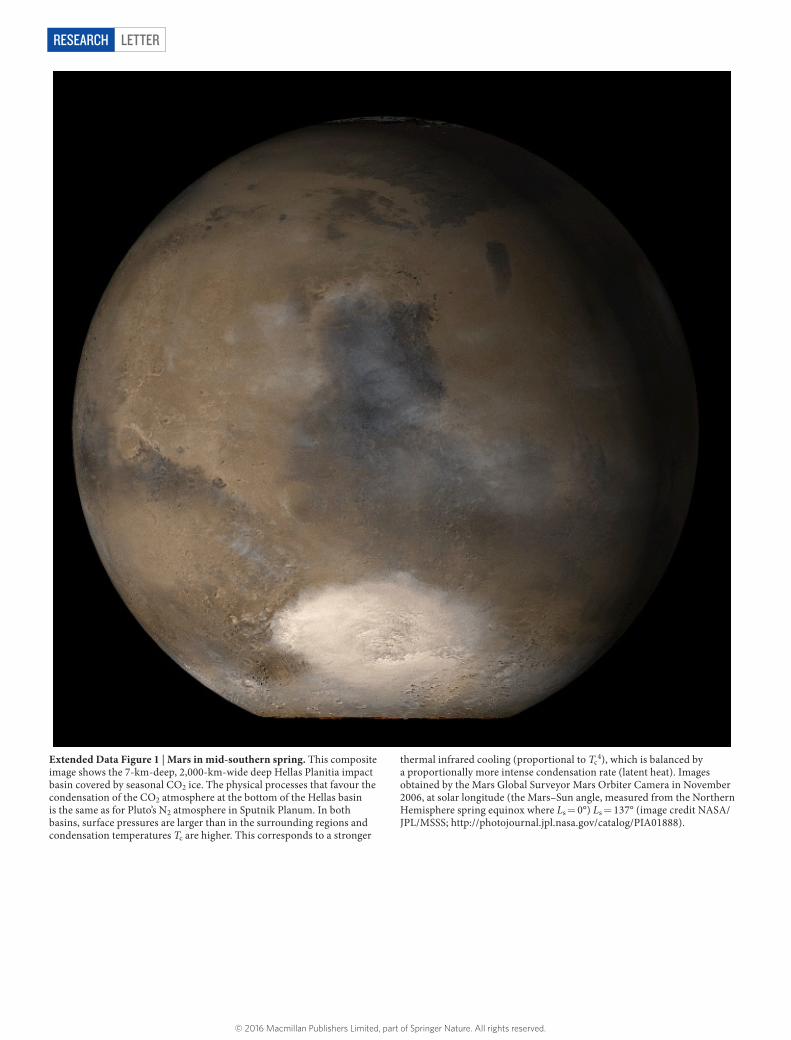
Extended Data Figure 2 | Evolution of surface pressure during the first 15,000 Earth years of the reference simulation (same as Fig. 1). At least 10,000 Earth years are necessary to equilibrate the N2 ice in the basin and obtain a year-to-year repetitive pattern of surface pressure.


LETTERRESEARCH

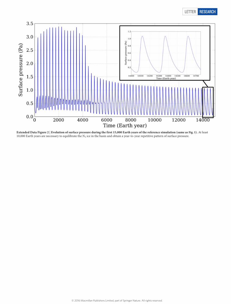
Extended Data Figure 3 | Latitudinal distribution of CH4 ice over three Pluto years in our reference simulation, as in Figs 1 and 2. The colour scale measures methane ice on the surface, in kilograms per square metre. The time axis starts at the solar longitude Ls = 0°. In addition to the permanent methane ice reservoir in the Sputnik Planum basin, the methane cycle exhibits seasonal polar frosts of methane. The southern

polar frosts remain in place longer than the northern frost, owing to the longer duration of the southern winter season. At mid-northern latitudes, the Sputnik Planum basin is a permanent reservoir of CH4 ice. CH4 frost preferentially accumulates at the poles during autumn and winter, but better resists sublimation at low latitudes during late spring, especially in the southern hemisphere.
