Embed Size (px)
Citation preview

ERCIM'11 - Handling imprecision in graphical models
Classification with decision trees from anonparametric predictive inference
perspective
Joaquín Abellán†, Rebecca M. Baker§, Frank P.A. Coolen§,Richard J. Crossman¶, Andrés. R. Masegosa†
† Department of Computer Science and Artificial Intelligence, University ofGranada, Granada, Spain
§ Department of Mathematical Sciences, Durham University, Durham, UK¶Warwick Medical School, University of Warwick, Coventry, UK
London, December 2011
ERCIM’11 London (UK) 1/28
Outline
1 Introduction
2 Imprecise Models for Multinomial data
3 Uncertainty Measures and Decision Trees
4 Experimental Evaluation
5 Conclusions & Future Works
ERCIM’11 London (UK) 2/28

Introduction
Part I
Introduction
ERCIM’11 London (UK) 3/28
Introduction
Imprecise Probabilities
Imprecise Probabilities is a term that subsumes severaltheories for reasoning under uncertainty:
Belief Functions
Reachable Probability Intervals
Capacities of various orders
Upper and lower probabilities
Credal Sets
.....
ERCIM’11 London (UK) 4/28
Introduction
Uncertainty Measures
Extensions of the classic information theory has beendeveloped for these imprecise models.
Several extensions to the Shannon entropy measure hasbeen proposed:
Maximum Entropy measure proposed by (Abellan - Moral,2003) as a total uncertainty measure for general credalsets.
The employment of this measure in the case of theImprecise Dirichlet model (IDM) has lead to severalsuccessful applications in the field of data-mining, speciallyon decision trees for supervised classification.
ERCIM’11 London (UK) 5/28

Introduction
Imprecise Dirichlet Model (IDM) model
The IDM model was proposed by Walley in 1996 forstatistical inference from multinomial data wasdeveloped to correct shortcomings of previous alternativeobjective models.
It verifies a set of principles which are claimed by Walleyto be desirable for inference:
Representation Invariance Principle.
It can be expressed via a set of reachable probabilityintervals and a belief function (Abellán,2006).
ERCIM’11 London (UK) 6/28
Introduction
Non-parametric Predictive Inference
Non-parametric Predictive Inference model for multinomial data (NPI-M) is
presented by (Coolen-Augustin,2005) as an alternative to the IDM model.
Learn from data in the absence of prior knowledge and with only a fewmodeling assumptions.Post-data exchangeability-like assumption together with a latentvariable representation of data.
BBB
B
P
P PP
P
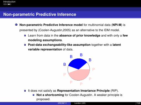
It does not satisfy as Representation Invariance Principle (RIP).Not a shortcoming for Coolen-Augustin. A weaker principle isproposed.
ERCIM’11 London (UK) 7/28
Introduction
Non-parametric Predictive Inference
Non-parametric Predictive Inference model for multinomial data (NPI-M) is
presented by (Coolen-Augustin,2005) as an alternative to the IDM model.
Learn from data in the absence of prior knowledge and with only a fewmodeling assumptions.
Post-data exchangeability-like assumption together with a latentvariable representation of data.
BBB
B
P
P PP
P
It does not satisfy as Representation Invariance Principle (RIP).Not a shortcoming for Coolen-Augustin. A weaker principle isproposed.
ERCIM’11 London (UK) 7/28

Introduction
Non-parametric Predictive Inference
Non-parametric Predictive Inference model for multinomial data (NPI-M) is
presented by (Coolen-Augustin,2005) as an alternative to the IDM model.
Learn from data in the absence of prior knowledge and with only a fewmodeling assumptions.Post-data exchangeability-like assumption together with a latentvariable representation of data.
BBB
B
P
P PP
P
It does not satisfy as Representation Invariance Principle (RIP).Not a shortcoming for Coolen-Augustin. A weaker principle isproposed.
ERCIM’11 London (UK) 7/28
Introduction
Classification with Decision Trees using NPI-M model
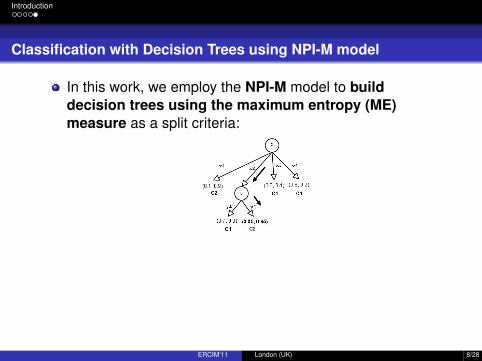
In this work, we employ the NPI-M model to builddecision trees using the maximum entropy (ME)measure as a split criteria:
We experimentally compare the decision trees build withIDM with different S values.
Classification accuracy is slightly improve.The decision trees are notably smaller.A parameter free method.
ERCIM’11 London (UK) 8/28

Introduction
Classification with Decision Trees using NPI-M model
In this work, we employ the NPI-M model to builddecision trees using the maximum entropy (ME)measure as a split criteria:
We experimentally compare the decision trees build withIDM with different S values.
Classification accuracy is slightly improve.The decision trees are notably smaller.A parameter free method.
ERCIM’11 London (UK) 8/28

Imprecise Models for Multinomial Data
Part II
Imprecise Models for MultinomialData
ERCIM’11 London (UK) 9/28

Imprecise Models for Multinomial Data
Imprecise Dirichlet Model
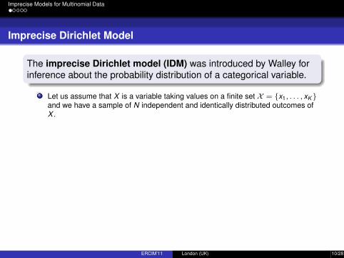
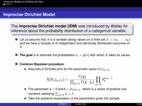
The imprecise Dirichlet model (IDM) was introduced by Walley forinference about the probability distribution of a categorical variable.
Let us assume that X is a variable taking values on a finite set X = {x1, . . . , xK }and we have a sample of N independent and identically distributed outcomes ofX .
The goal is to estimate the probabilities θx = p(x) with which X takes its values.
Common Bayesian procedure:
Assumes a Dirichlet prior for the parameter vector (θx )x∈X .
f ((θx )x∈X ) =Γ(s)∏
x∈X Γ(s · tx )
∏x∈X
θs·tx−1x
The parameter s > 0 and t = (tx )x∈X , which is a vector of positive realnumbers satisfying
∑x∈X tx = 1.
Take the posterior expectation of the parameters given the sample.
ERCIM’11 London (UK) 10/28
Imprecise Models for Multinomial Data
Imprecise Dirichlet Model
The imprecise Dirichlet model (IDM) was introduced by Walley forinference about the probability distribution of a categorical variable.
Let us assume that X is a variable taking values on a finite set X = {x1, . . . , xK }and we have a sample of N independent and identically distributed outcomes ofX .
The goal is to estimate the probabilities θx = p(x) with which X takes its values.
Common Bayesian procedure:
Assumes a Dirichlet prior for the parameter vector (θx )x∈X .
f ((θx )x∈X ) =Γ(s)∏
x∈X Γ(s · tx )
∏x∈X
θs·tx−1x
The parameter s > 0 and t = (tx )x∈X , which is a vector of positive realnumbers satisfying
∑x∈X tx = 1.
Take the posterior expectation of the parameters given the sample.
ERCIM’11 London (UK) 10/28
Imprecise Models for Multinomial Data
Imprecise Dirichlet Model
The imprecise Dirichlet model (IDM) was introduced by Walley forinference about the probability distribution of a categorical variable.
Let us assume that X is a variable taking values on a finite set X = {x1, . . . , xK }and we have a sample of N independent and identically distributed outcomes ofX .
The goal is to estimate the probabilities θx = p(x) with which X takes its values.
Common Bayesian procedure:
Assumes a Dirichlet prior for the parameter vector (θx )x∈X .
f ((θx )x∈X ) =Γ(s)∏
x∈X Γ(s · tx )
∏x∈X
θs·tx−1x
The parameter s > 0 and t = (tx )x∈X , which is a vector of positive realnumbers satisfying
∑x∈X tx = 1.
Take the posterior expectation of the parameters given the sample.ERCIM’11 London (UK) 10/28
Imprecise Models for Multinomial Data
Imprecise Dirichlet Model
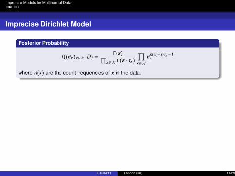
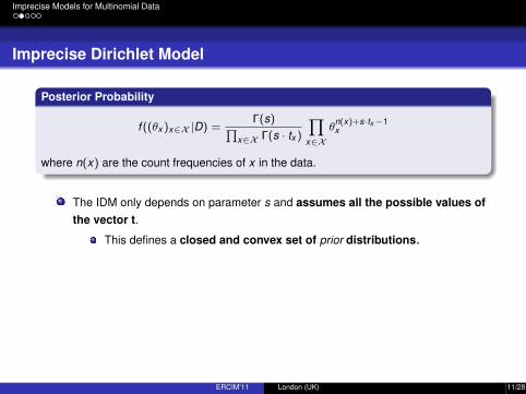
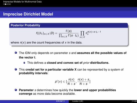
Posterior Probability
f ((θx )x∈X |D) =Γ(s)∏
x∈X Γ(s · tx )
∏x∈X
θn(x)+s·tx−1x
where n(x) are the count frequencies of x in the data.
The IDM only depends on parameter s and assumes all the possible values ofthe vector t.
This defines a closed and convex set of prior distributions.
This credal set for a particular variable X can be represented by a system ofprobability intervals:
p′(x) ∈ [n(x)
N + s,
n(x) + sN + s
]
Parameter s determines how quickly the lower and upper probabilitiesconverge as more data become available.
ERCIM’11 London (UK) 11/28
Imprecise Models for Multinomial Data
Imprecise Dirichlet Model
Posterior Probability
f ((θx )x∈X |D) =Γ(s)∏
x∈X Γ(s · tx )
∏x∈X
θn(x)+s·tx−1x
where n(x) are the count frequencies of x in the data.
The IDM only depends on parameter s and assumes all the possible values ofthe vector t.
This defines a closed and convex set of prior distributions.
This credal set for a particular variable X can be represented by a system ofprobability intervals:
p′(x) ∈ [n(x)
N + s,
n(x) + sN + s
]
Parameter s determines how quickly the lower and upper probabilitiesconverge as more data become available.
ERCIM’11 London (UK) 11/28
Imprecise Models for Multinomial Data
The NPI-M model
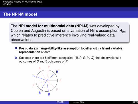
The NPI model for multinomial data (NPI-M) was developed byCoolen and Augustin is based on a variation of Hill’s assumption A(n)
which relates to predictive inference involving real-valued dataobservations.
Post-data exchangeability-like assumption together with a latent variablerepresentation of data.
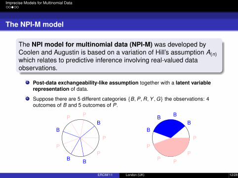
Suppose there are 5 different categories {B,P,R,Y ,G} the observations: 4outcomes of B and 5 outcomes of P.
B
PP
B
P
B B
P
P
B
BB
B
P
P P
P
P
ERCIM’11 London (UK) 12/28
Imprecise Models for Multinomial Data
The NPI-M model
The NPI model for multinomial data (NPI-M) was developed byCoolen and Augustin is based on a variation of Hill’s assumption A(n)
which relates to predictive inference involving real-valued dataobservations.
Post-data exchangeability-like assumption together with a latent variablerepresentation of data.
Suppose there are 5 different categories {B,P,R,Y ,G} the observations: 4outcomes of B and 5 outcomes of P.
B
PP
B
P
B B
P
P
B
BB
B
P
P P
P
P
ERCIM’11 London (UK) 12/28

Imprecise Models for Multinomial Data
The NPI-M model
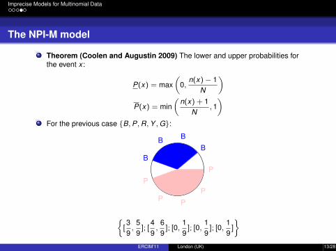
Theorem (Coolen and Augustin 2009) The lower and upper probabilities forthe event x :
P(x) = max(
0,n(x)− 1
N
)P(x) = min
(n(x) + 1
N, 1)
For the previous case {B,P,R,Y ,G}:
B
BB
B
P
P P
P
P
{[39,
59
]; [49,
69
]; [0,19
]; [0,19
]; [0,19
]
}
ERCIM’11 London (UK) 13/28
Imprecise Models for Multinomial Data
The NPI-M model
Theorem (Coolen and Augustin 2009) The lower and upper probabilities forthe event x :
P(x) = max(
0,n(x)− 1
N
)P(x) = min
(n(x) + 1
N, 1)
For the previous case {B,P,R,Y ,G}:
B
BB
B
P
P P
P
P
{[39,
59
]; [49,
69
]; [0,19
]; [0,19
]; [0,19
]
}ERCIM’11 London (UK) 13/28
Imprecise Models for Multinomial Data
The A-NPI-M model
This set of lower and upper probabilities,L, associated with the singleton eventsx expresses a reachable set of probability intervals, i.e. a credal set.
L = {[max(
0,n(x)− 1
N
),min
(n(x) + 1
N, 1)
] : x ∈ {x1, ..., xK }}
The set of probability distributions obtained from NPI-M is not a credal set (seea counterexample in the paper).
p = ( 39 ,
49 ,
227 ,
227 ,
227 ) belongs to the credal set:{
[ 39 ,
59 ]; [ 4
9 ,69 ]; [0, 1
9 ]; [0, 19 ]; [0, 1
9 ]}
It is not possible to find a configuration of the probability wheel thatcorresponds to p.
The A-NPI-M model is a simplified approximate model derived from NPI-M byconsidering all probability distributions compatible with the set of lower and upperprobabilities, L, obtained from NPI-M.
ERCIM’11 London (UK) 14/28
Imprecise Models for Multinomial Data
The A-NPI-M model
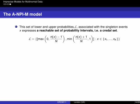
This set of lower and upper probabilities,L, associated with the singleton eventsx expresses a reachable set of probability intervals, i.e. a credal set.
L = {[max(
0,n(x)− 1
N
),min
(n(x) + 1
N, 1)
] : x ∈ {x1, ..., xK }}
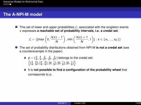
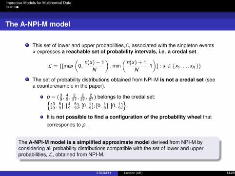
The set of probability distributions obtained from NPI-M is not a credal set (seea counterexample in the paper).
p = ( 39 ,
49 ,
227 ,
227 ,
227 ) belongs to the credal set:{
[ 39 ,
59 ]; [ 4
9 ,69 ]; [0, 1
9 ]; [0, 19 ]; [0, 1
9 ]}
It is not possible to find a configuration of the probability wheel thatcorresponds to p.
The A-NPI-M model is a simplified approximate model derived from NPI-M byconsidering all probability distributions compatible with the set of lower and upperprobabilities, L, obtained from NPI-M.
ERCIM’11 London (UK) 14/28
Imprecise Models for Multinomial Data
The A-NPI-M model
This set of lower and upper probabilities,L, associated with the singleton eventsx expresses a reachable set of probability intervals, i.e. a credal set.
L = {[max(
0,n(x)− 1
N
),min
(n(x) + 1
N, 1)
] : x ∈ {x1, ..., xK }}
The set of probability distributions obtained from NPI-M is not a credal set (seea counterexample in the paper).
p = ( 39 ,
49 ,
227 ,
227 ,
227 ) belongs to the credal set:{
[ 39 ,
59 ]; [ 4
9 ,69 ]; [0, 1
9 ]; [0, 19 ]; [0, 1
9 ]}
It is not possible to find a configuration of the probability wheel thatcorresponds to p.
The A-NPI-M model is a simplified approximate model derived from NPI-M byconsidering all probability distributions compatible with the set of lower and upperprobabilities, L, obtained from NPI-M.
ERCIM’11 London (UK) 14/28

Uncertainty Measures and Decision Trees
Part III
Uncertainty Measures andDecision Trees
ERCIM’11 London (UK) 15/28

Uncertainty Measures and Decision Trees
Decision Trees
A decision tree, also called a classification tree, is a simple structure that canbe used as a classifier.
Each node represents an attribute variable
Each branch represents one of the states of this variable
Each tree leaf specifies an expected value of the class variable
Example of decision tree for three attribute variables Ai (i = 1, 2, 3), with twopossible values (0, 1) and a class variable C with cases or states c1, c2, c3:
ERCIM’11 London (UK) 16/28
Uncertainty Measures and Decision Trees
Building Decision Trees from data
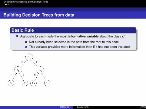
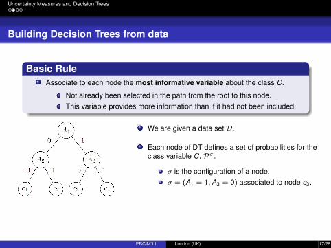
Basic RuleAssociate to each node the most informative variable about the class C.
Not already been selected in the path from the root to this node.This variable provides more information than if it had not been included.
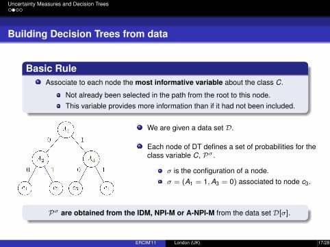
We are given a data set D.
Each node of DT defines a set of probabilities for theclass variable C, Pσ .
σ is the configuration of a node.σ = (A1 = 1,A3 = 0) associated to node c3.
Pσ are obtained from the IDM, NPI-M or A-NPI-M from the data set D[σ].
ERCIM’11 London (UK) 17/28
Uncertainty Measures and Decision Trees
Building Decision Trees from data
Basic RuleAssociate to each node the most informative variable about the class C.
Not already been selected in the path from the root to this node.This variable provides more information than if it had not been included.
We are given a data set D.
Each node of DT defines a set of probabilities for theclass variable C, Pσ .
σ is the configuration of a node.σ = (A1 = 1,A3 = 0) associated to node c3.
Pσ are obtained from the IDM, NPI-M or A-NPI-M from the data set D[σ].
ERCIM’11 London (UK) 17/28
Uncertainty Measures and Decision Trees
Imprecise Information Gain
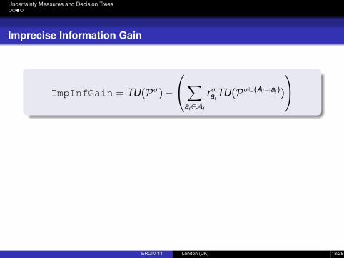
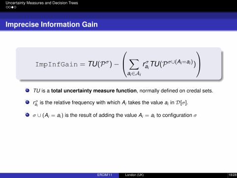
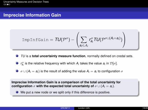
ImpInfGain = TU(Pσ)−
∑ai∈Ai
rσaiTU(Pσ∪(Ai =ai ))
TU is a total uncertainty measure function, normally defined on credal sets.
rσaiis the relative frequency with which Ai takes the value ai in D[σ].
σ ∪ (Ai = ai ) is the result of adding the value Ai = ai to configuration σ
Imprecise Information Gain is a comparison of the total uncertainty forconfiguration σ with the expected total uncertainty of σ ∪ (Ai = ai ).
We put a new node or we split only if this difference is positive.
ERCIM’11 London (UK) 18/28
Uncertainty Measures and Decision Trees
Imprecise Information Gain
ImpInfGain = TU(Pσ)−
∑ai∈Ai
rσaiTU(Pσ∪(Ai =ai ))
TU is a total uncertainty measure function, normally defined on credal sets.
rσaiis the relative frequency with which Ai takes the value ai in D[σ].
σ ∪ (Ai = ai ) is the result of adding the value Ai = ai to configuration σ
Imprecise Information Gain is a comparison of the total uncertainty forconfiguration σ with the expected total uncertainty of σ ∪ (Ai = ai ).
We put a new node or we split only if this difference is positive.
ERCIM’11 London (UK) 18/28

Uncertainty Measures and Decision Trees
Maximum Entropy
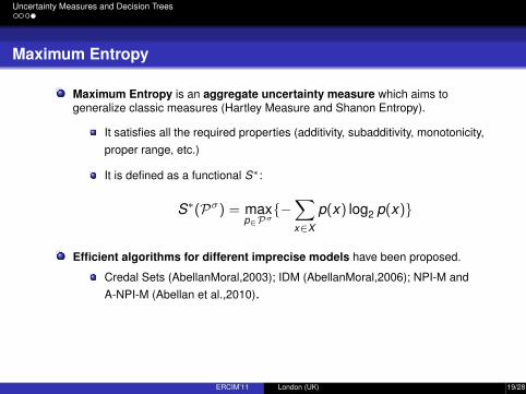
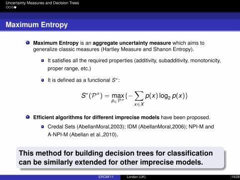
Maximum Entropy is an aggregate uncertainty measure which aims togeneralize classic measures (Hartley Measure and Shanon Entropy).
It satisfies all the required properties (additivity, subadditivity, monotonicity,proper range, etc.)
It is defined as a functional S∗:
S∗(Pσ) = maxp∈Pσ
{−∑x∈X
p(x) log2 p(x)}
Efficient algorithms for different imprecise models have been proposed.
Credal Sets (AbellanMoral,2003); IDM (AbellanMoral,2006); NPI-M andA-NPI-M (Abellan et al.,2010).
This method for building decision trees for classificationcan be similarly extended for other imprecise models.
ERCIM’11 London (UK) 19/28
Uncertainty Measures and Decision Trees
Maximum Entropy
Maximum Entropy is an aggregate uncertainty measure which aims togeneralize classic measures (Hartley Measure and Shanon Entropy).
It satisfies all the required properties (additivity, subadditivity, monotonicity,proper range, etc.)
It is defined as a functional S∗:
S∗(Pσ) = maxp∈Pσ
{−∑x∈X
p(x) log2 p(x)}
Efficient algorithms for different imprecise models have been proposed.
Credal Sets (AbellanMoral,2003); IDM (AbellanMoral,2006); NPI-M andA-NPI-M (Abellan et al.,2010).
This method for building decision trees for classificationcan be similarly extended for other imprecise models.
ERCIM’11 London (UK) 19/28

Experimental Evaluation
Part IV
Experimental Evaluation
ERCIM’11 London (UK) 20/28

Experimental Evaluation
Experimental Set-up
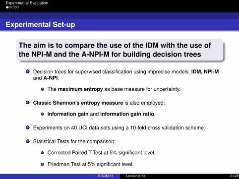
The aim is to compare the use of the IDM with the use ofthe NPI-M and the A-NPI-M for building decision trees
Decision trees for supervised classification using imprecise models, IDM, NPI-Mand A-NPI:
The maximum entropy as base measure for uncertainty.
Classic Shannon’s entropy measure is also employed:
information gain and information gain ratio.
Experiments on 40 UCI data sets using a 10-fold-cross validation scheme.
Statistical Tests for the comparison:
Corrected Paired T-Test at 5% significant level.
Friedman Test at 5% significant level.
ERCIM’11 London (UK) 21/28
Experimental Evaluation
Experimental Set-up
The aim is to compare the use of the IDM with the use ofthe NPI-M and the A-NPI-M for building decision trees
Decision trees for supervised classification using imprecise models, IDM, NPI-Mand A-NPI:
The maximum entropy as base measure for uncertainty.
Classic Shannon’s entropy measure is also employed:
information gain and information gain ratio.
Experiments on 40 UCI data sets using a 10-fold-cross validation scheme.
Statistical Tests for the comparison:
Corrected Paired T-Test at 5% significant level.
Friedman Test at 5% significant level.
ERCIM’11 London (UK) 21/28
Experimental Evaluation
Evaluating Classification Accuracy
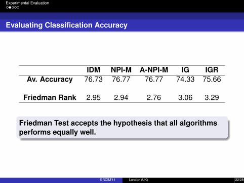
IDM NPI-M A-NPI-M IG IGRAv. Accuracy 76.73 76.77 76.77 74.33 75.66
Friedman Rank 2.95 2.94 2.76 3.06 3.29
Friedman Test accepts the hypothesis that all algorithmsperforms equally well.
ERCIM’11 London (UK) 22/28
Experimental Evaluation
Evaluating the size of the decision trees
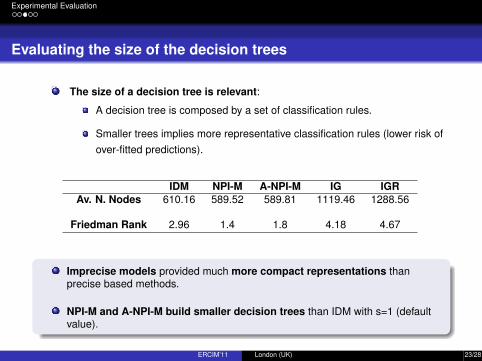
The size of a decision tree is relevant:
A decision tree is composed by a set of classification rules.
Smaller trees implies more representative classification rules (lower risk ofover-fitted predictions).
IDM NPI-M A-NPI-M IG IGRAv. N. Nodes 610.16 589.52 589.81 1119.46 1288.56
Friedman Rank 2.96 1.4 1.8 4.18 4.67
Imprecise models provided much more compact representations thanprecise based methods.
NPI-M and A-NPI-M build smaller decision trees than IDM with s=1 (defaultvalue).
ERCIM’11 London (UK) 23/28
Experimental Evaluation
Evaluating the size of the decision trees
The size of a decision tree is relevant:
A decision tree is composed by a set of classification rules.
Smaller trees implies more representative classification rules (lower risk ofover-fitted predictions).
IDM NPI-M A-NPI-M IG IGRAv. N. Nodes 610.16 589.52 589.81 1119.46 1288.56
Friedman Rank 2.96 1.4 1.8 4.18 4.67
Imprecise models provided much more compact representations thanprecise based methods.
NPI-M and A-NPI-M build smaller decision trees than IDM with s=1 (defaultvalue).
ERCIM’11 London (UK) 23/28
Experimental Evaluation
Evaluating IDM with different s values
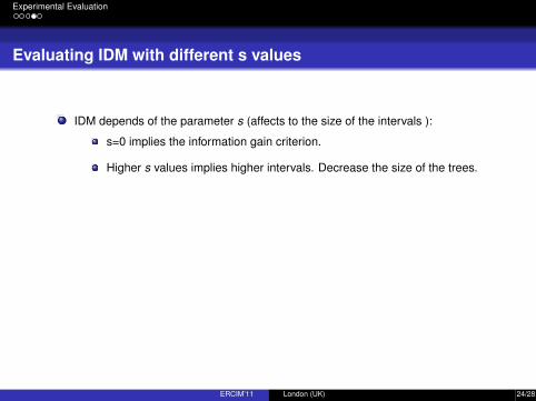
IDM depends of the parameter s (affects to the size of the intervals ):
s=0 implies the information gain criterion.
Higher s values implies higher intervals. Decrease the size of the trees.
NPI-M IDM-S1 IDM-S1.5 IDM-S2.0Av. N. Nodes 589.5 610.2 480.3 383.8
Friedman Rank 2.4 3.85 2.43 1.28
IDM with s=1.5 obtains decision trees with a similar size to NPI-M.
IDM with s=2.0 obtains decision trees with smaller similar size than NPI-M.
ERCIM’11 London (UK) 24/28

Experimental Evaluation
Evaluating IDM with different s values
IDM depends of the parameter s (affects to the size of the intervals ):
s=0 implies the information gain criterion.
Higher s values implies higher intervals. Decrease the size of the trees.
NPI-M IDM-S1 IDM-S1.5 IDM-S2.0Av. N. Nodes 589.5 610.2 480.3 383.8
Friedman Rank 2.4 3.85 2.43 1.28
IDM with s=1.5 obtains decision trees with a similar size to NPI-M.
IDM with s=2.0 obtains decision trees with smaller similar size than NPI-M.
ERCIM’11 London (UK) 24/28
Experimental Evaluation
Evaluating IDM with different s values
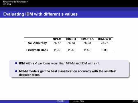
NPI-M IDM-S1 IDM-S1.5 IDM-S2.0Av. Accuracy 76.77 76.73 76.23 75.75
Friedman Rank 2.25 2.26 2.46 3.03
IDM with s>1 performs worst than NPI-M and IDM with s=1.
NPI-M models get the best classification accuracy with the smallestdecision trees.
ERCIM’11 London (UK) 25/28

Conclusions and Future Works
Part V
Conclusions and Future Works
ERCIM’11 London (UK) 26/28
Conclusions and Future Works
Conclusions and Future Works
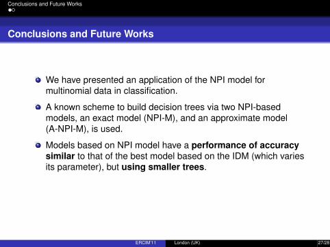
We have presented an application of the NPI model formultinomial data in classification.
A known scheme to build decision trees via two NPI-basedmodels, an exact model (NPI-M), and an approximate model(A-NPI-M), is used.
Models based on NPI model have a performance of accuracysimilar to that of the best model based on the IDM (which variesits parameter), but using smaller trees.
Future Works:
Extend these methods for credal classification.
ERCIM’11 London (UK) 27/28
Conclusions and Future Works
Conclusions and Future Works
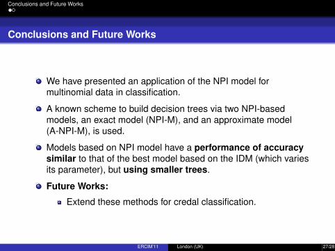
We have presented an application of the NPI model formultinomial data in classification.
A known scheme to build decision trees via two NPI-basedmodels, an exact model (NPI-M), and an approximate model(A-NPI-M), is used.
Models based on NPI model have a performance of accuracysimilar to that of the best model based on the IDM (which variesits parameter), but using smaller trees.
Future Works:
Extend these methods for credal classification.
ERCIM’11 London (UK) 27/28

Conclusions and Future Works
Thanks for you attention!
Questions?
ERCIM’11 London (UK) 28/28