ICDE 2015 - LDV: Light-weight Database Virtualization

LDV: Light-weight Database VirtualizationQuan Pham2, Tanu Malik1, Boris Glavic3 and Ian Foster1,2

Computation Institute1and Department of Computer Science2,3

University of Chicago1,2, Argonne National Laboratory1

Illinois Institute of Technology3

Share and Reproduce

Alice wants to share her models and simulation output with Bob, and Bob wants to re-execute Alice’s application to validate her inputs and outputs.

Alice Bob

Significance

|

re

po

rtin

g c

he

cklis

t fo

r lif

e s

cie

nc

es

a

rtic

les

May 2013

i

1. How was the sample size chosen to ensure adequate power to detect a pre-specified effect size?

For animal studies, include a statement about sample size estimate even if no statistical methods were used.

2. Describe inclusion/exclusion criteria if samples or animals were excluded from the analysis. Were the criteria pre-established?

3. If a method of randomization was used to determine how samples/animals were allocated to experimental groups and processed, describe it.

For animal studies, include a statement about randomization even if no randomization was used.

4. If the investigator was blinded to the group allocation during the experiment and/or when assessing the outcome, state the extent of blinding.

For animal studies, include a statement about blinding even if no blinding was done.

5. For every figure, are statistical tests justified as appropriate?

Do the data meet the assumptions of the tests (e.g., normal distribution)?

Is there an estimate of variation within each group of data? Is the variance similar between the groups that are being statistically compared?

Reporting Checklist For Life Sciences ArticlesThis checklist is used to ensure good reporting standards and to improve the reproducibility of published results. For more information, please read Reporting Life Sciences Research.

` Figure legendsEach figure legend should contain, for each panel where they are relevant:

the exact sample size (n) for each experimental group/condition, given as a number, not a range; a description of the sample collection allowing the reader to understand whether the samples represent technical or biological

replicates (including how many animals, litters, cultures, etc.); a statement of how many times the experiment shown was replicated in the laboratory; definitions of statistical methods and measures:

○ very common tests, such as t-test, simple χ2 tests, Wilcoxon and Mann-Whitney tests, can be unambiguously identified by name only, but more complex techniques should be described in the methods section;

○ are tests one-sided or two-sided?○ are there adjustments for multiple comparisons?○ statistical test results, e.g., P values;○ definition of ‘center values’ as median or average; ○ definition of error bars as s.d. or s.e.m.

Any descriptions too long for the figure legend should be included in the methods section.

Please ensure that the answers to the following questions are reported in the manuscript itself. We encourage you to include a specific subsection in the methods section for statistics, reagents and animal models. Below, provide the page number(s) or figure legend(s) where the information can be located.

` Statistics and general methodsReported on page(s) or figure legend(s):

Corresponding Author Name: ________________________________________

Manuscript Number: ______________________________

(Continues on following page)

Metrics aims to improve the reproducibility of scientific research.

NY Times, Dec, 2014

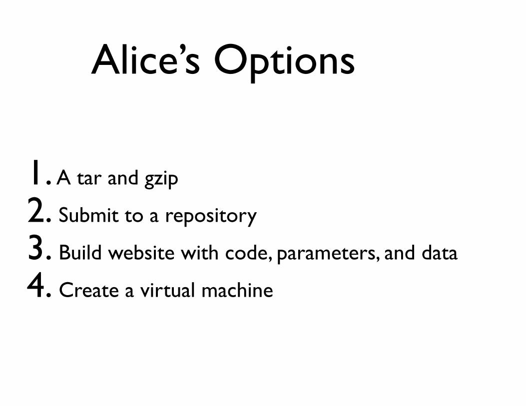
Alice’s Options

1. A tar and gzip

2. Submit to a repository

3. Build website with code, parameters, and data

4. Create a virtual machine

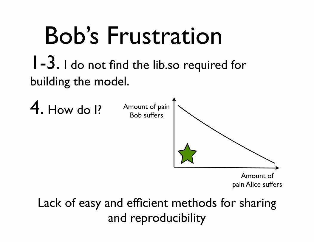
Bob’s Frustration1-3. I do not find the lib.so required for building the model.

4. How do I?

Lack of easy and efficient methods for sharing and reproducibility

Amount of pain Bob suffers

Amount of pain Alice suffers

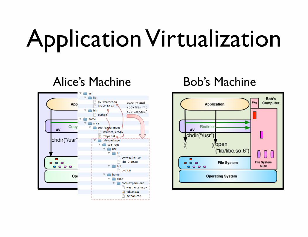
Application Virtualization

Alice’s Machine Bob’s Machine&RGH�'DWD�(QYLURQPHQW

$XGLWƔ ,QYRNH�DORQJVLGH�WKH�FRPSXWDWLRQ

FGH�S\WKRQ�ZHDWKHUBVLP�S\�WRN\R�GDW

Ɣ &DSWXUHV�V\VWHP�FDOOV�XVLQJSWUDFHż ([HFXWH�DQG�FRS\�LQWR�FGH�SDFNDJH�FGH�URRW

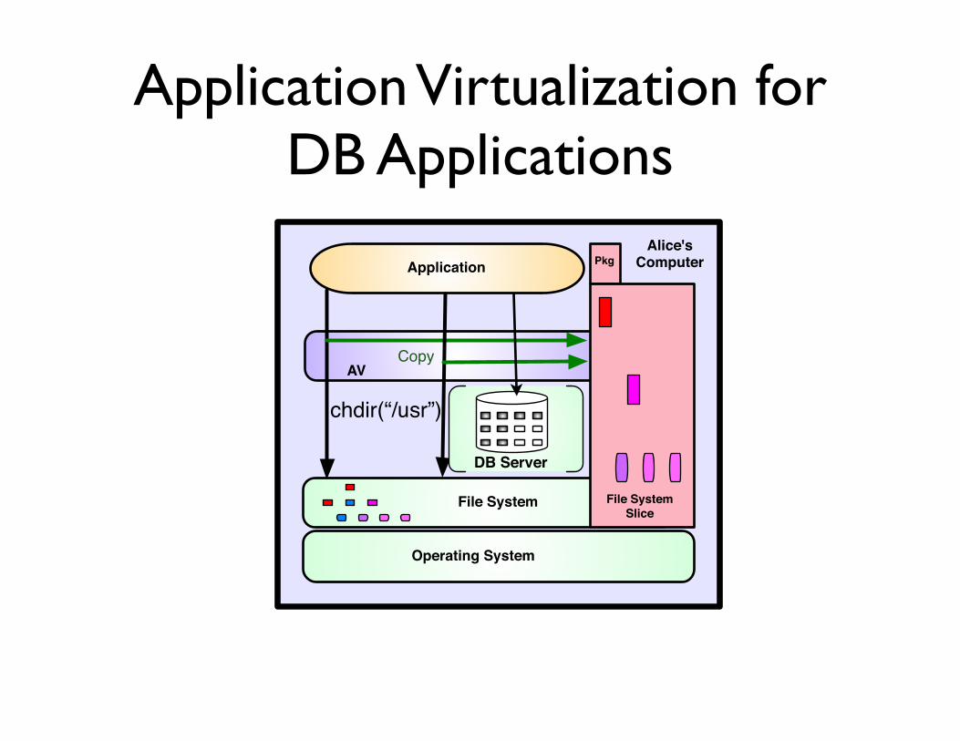
Application Virtualization for DB Applications

Application

Operating System

File System File System Slice

Pkg

Copy AV

Alice'sComputer

chdir(“/usr”)open(“lib/libc.so.6”)DB Server

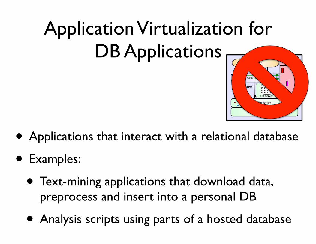
Application Virtualization for DB Applications

• Applications that interact with a relational database

• Examples:

• Text-mining applications that download data, preprocess and insert into a personal DB

• Analysis scripts using parts of a hosted database

Application

Operating System

File System File System Slice

Pkg

Copy AV

Alice'sComputer

chdir(“/usr”)open(“lib/libc.so.6”)DB Server

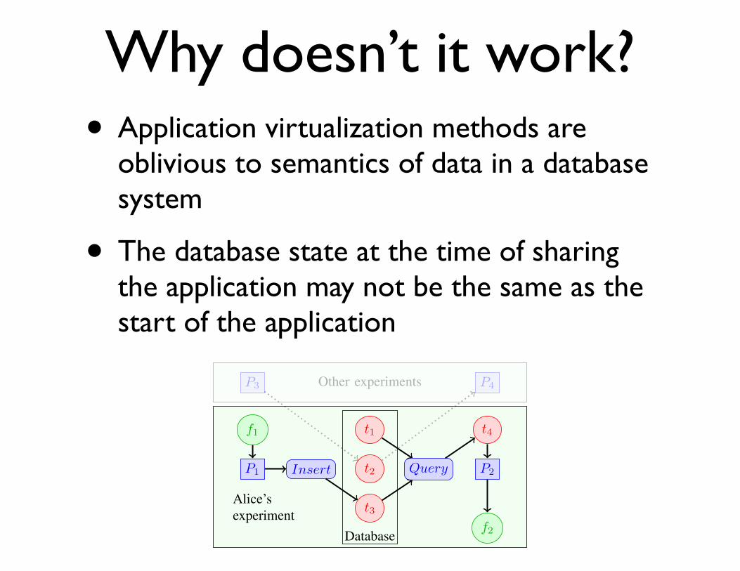
Why doesn’t it work?• Application virtualization methods are

oblivious to semantics of data in a database system

• The database state at the time of sharing the application may not be the same as the start of the application

• Databases are often shared among multiple users andacross many application. Thus, to re-execute an applica-tion, the database state, as of the start of the application,has to be restored.

• Provenance can be used to understand a shared applica-tion. While database and application provenance are wellunderstood, combining these two types of provenanceremains challenging.

None of the above mentioned methods - companion web-sites, VM images, and application virtualization - addressesthese challenges. There is no automatic mechanism for cap-turing and linking application and DB provenance, theseapproaches provide no means for determining which data isrelevant for an application, they do not solve the issue ofresetting a database to a previous state, and do not addressthe licensing problem of sharing the binaries of commercialdatabase servers.

For example, application virtualization is currently limitedto local applications that do not communicate to server pro-cesses, such as a web server or a database server. In fact,when an application communicates with a database server,the technique can atmost record the communication betweenthe client and database server. This is not sufficient fordetermining which data was used by the application (and, thus,should be included in the package) and to be able to resetthe database to its state before application execution started.Temporal databases provide a solution for the later problem,but not for the earlier. Virtualization can ensure reproducibilityif the user has control over the database server, the serveris started as part of the application (thus the virtualizationsystem can capture a consistent state of the database files ondisk and the server binaries) and shutdown before the capturemechanism is stopped. However, this will include completedatabase into the resulting package.

The goal of this work is to improve computational repro-ducibility for database applications. The light-weight databaseapplication virtualization (LDV) approach we present in thiswork addresses the aforementioned challenges. In particular,LDV enables users to easily create a light-weight databaseapplication virtualization (LDV) package, consisting of code,data, software dependencies, a slice of the database with whichis required for re-execution, and provenance. If shared witha 2nd party, the application runs in exactly the same wayas it did for the original user, without requiring installationor configuration of a database server at the target site. Theprovenance included in a package can used to understanddata dependencies across the application and database, and todetermine which parts of a workflow are needed to re-createa partial result.

II. LIGHT-WEIGHT DATABASE VIRTUALIZATION

We describe our approach by means of an example repro-ducibility task. Consider a user Alice who has been using adatabase in the past to conduct her experiments. She has finallydeveloped a database application which reads some input dataand outputs some analysis that she believes is interesting to

share with Bob (Figure 1). Alice would preferably like to sharethis application in the form of package P with Bob, who maywant to re-execute the application in its entirety or may want tovalidate, just the analysis task, or provide his own data inputsto examine the analysis result.

If Alice wants Bob to re-execute and build upon herdatabase application, then Bob must have access to an en-vironment that consists of application binaries and data, anyextension modules that the code depends upon (e.g., dynam-ically linked libraries), a database server and a database onwhich the application can be re-executed. Ideally, it wouldbe useful if Alice’s environment can be virtualized and thusautomatically set up for Bob.

P3 P4Other experiments

f1

P1 Insert

t1

t2

t3

Query

P2

t4

f2

Alice’sexperiment

Database

Fig. 1: Alice’s experiment with processes P1 and P2 uses tuplet1, inserts tuple t3, creates final output f2. Dumping databaseproduces redundant tuple t2. Capturing Alice’s experiment inits fullness makes t3 redundant. Only t1 is needed for theexperiment to execute.

If we assume that Alice’s application consists of set ofmodules that read data from files and/or retrieve data froma database, and write data to files and/or write data to adatabase, the database server is accessed through standardSQL language commands, and Alice executes her applicationthrough a command line script, providing a single entry pointfor monitoring the application, then several questions arisewith respect to virtualizing her environment. In particular:

•How do we include the necessary and sufficient data, i.e.,data that corresponds to her last experiment in the virtualizedenvironment? As Figure 1 shows there are data (tuples) in thedatabase that are not part of the current experiment and ifincluded in the package, may increase the size considerably,not leading to a light-weight virtualized environment.

•How can a self-contained package be created so that Bobdoes not have to install or configure a database server?

•How can Bob re-execute the database application, par-tially, or wholly, without communicating with Alice’s databaseserver?

We describe our primary contributions in addressing thesequestions, and also describe an overall organization map forthe paper. In summary we monitor database applications andcombine database and application provenance to determinenecessary and sufficient data. We describe how this data can be

LDV: Light-weight Database Virtualization

• Goal: Easily and efficiently share and repeat DB applications.

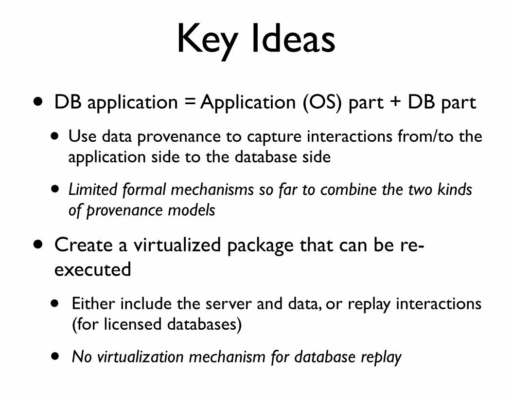
Key Ideas

• DB application = Application (OS) part + DB part

• Use data provenance to capture interactions from/to the application side to the database side

• Limited formal mechanisms so far to combine the two kinds of provenance models

• Create a virtualized package that can be re-executed

• Either include the server and data, or replay interactions (for licensed databases)

• No virtualization mechanism for database replay

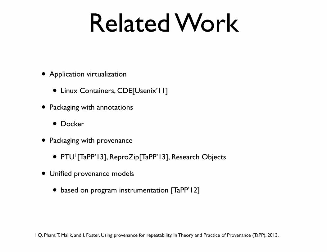
Related Work

• Application virtualization

• Linux Containers, CDE[Usenix’11]

• Packaging with annotations

• Docker

• Packaging with provenance

• PTU1[TaPP’13], ReproZip[TaPP’13], Research Objects

• Unified provenance models

• based on program instrumentation [TaPP’12]

1 Q. Pham, T. Malik, and I. Foster. Using provenance for repeatability. In Theory and Practice of Provenance (TaPP), 2013.

How does LDV work?

Application

Operating System

File System

DB Server

Execution Trace

DB Server DB Slice

File System Slice

Pkg

Copy LDV

Alice'sComputer

Alice’s Machine

ldv-audit db-app

• Monitoring system calls

• Monitoring SQL

• Server-included packages

• Server-excluded packages

• Execution traces

• Relevant DB and filesystem slices

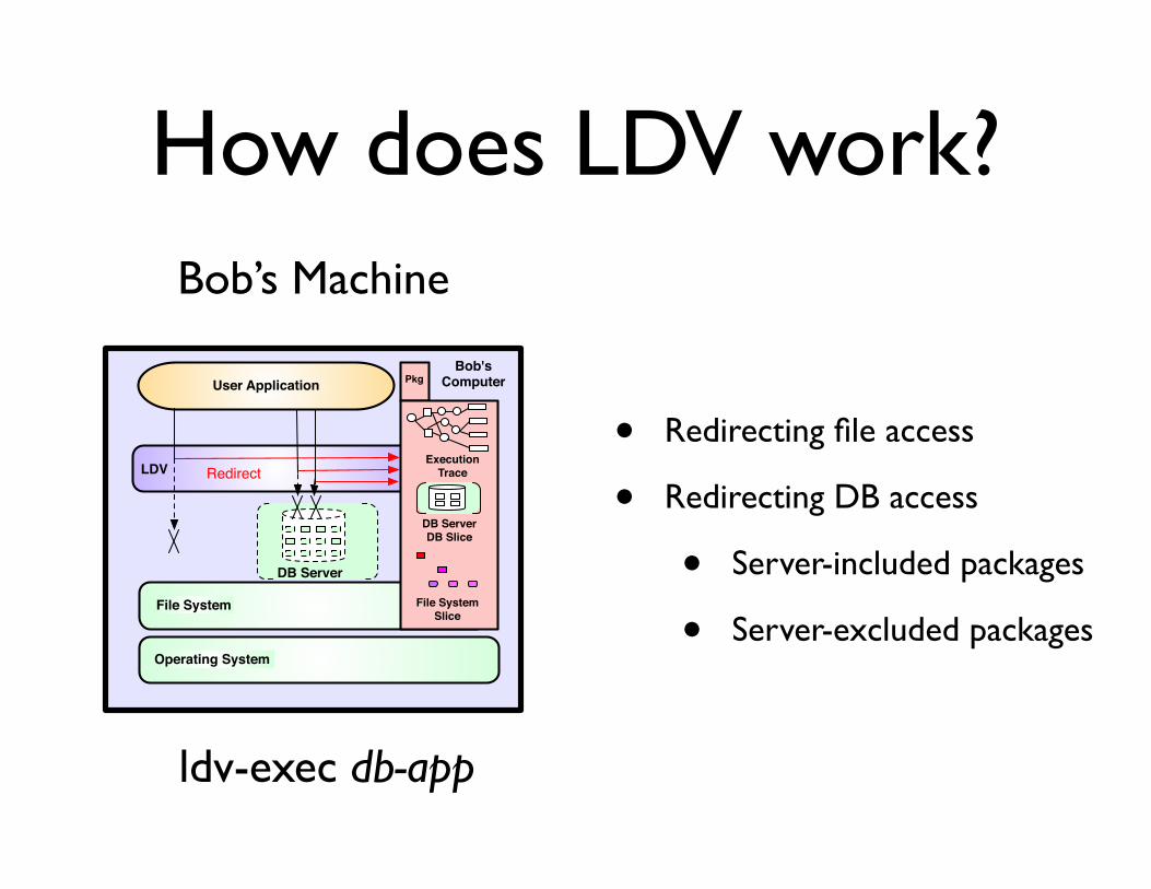
• Redirecting file access

• Redirecting DB access


• Server-excluded packagesFile System

Bob'sComputerUser Application

Operating System

DB Server

Execution Trace

DB Server DB Slice

File System Slice

Pkg

LDV Redirect

Bob’s Machine

ldv-exec db-app

How does LDV work?

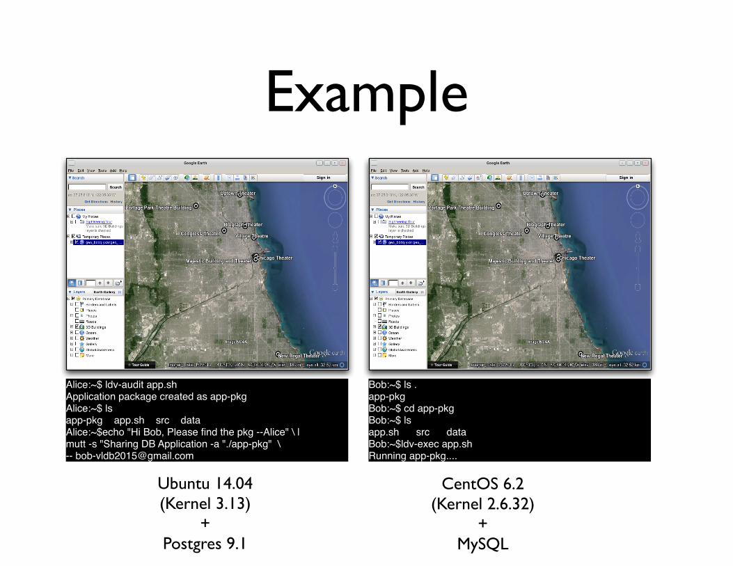
Example

Alice:~$ ldv-audit app.shApplication package created as app-pkgAlice:~$ lsapp-pkg app.sh src dataAlice:~$echo "Hi Bob, Please find the pkg --Alice" \ | mutt -s "Sharing DB Application -a "./app-pkg" \ -- [email protected]

Bob:~$ ls .app-pkgBob:~$ cd app-pkgBob:~$ lsapp.sh src dataBob:~$ldv-exec app.shRunning app-pkg....

Ubuntu 14.04(Kernel 3.13)

+Postgres 9.1

CentOS 6.2(Kernel 2.6.32)

+MySQL

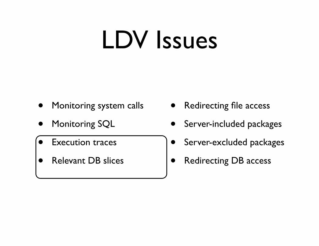
LDV Issues

• Monitoring system calls

• Monitoring SQL

• Execution traces

• Relevant DB slices

• Redirecting file access


• Server-excluded packages

• Redirecting DB access

An Execution Trace

A B

P1

Insert1

Insert2

t1

t2

t3

Query

t4

t5

P2

C[1, 6] [7, 8]

[5, 5]

[8, 8]

[5, 5]

[5, 5]

[8, 8]

[9, 9]

[9, 9]

[9, 9]

[9, 9]

[9, 9]

[9, 9]

[9, 9]

[7, 12]

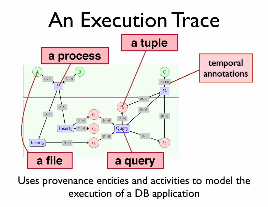
Fig. 2: An execution trace with processes and database operations

t1

t2

t3

Q1 t4

[4, 4]

[4, 4]

[4, 4]

[4, 4]

Fig. 3: PLin trace and data dependencies.

A

BP1

C

D

[1, 5]

[5, 7]

[2, 3]

[8, 8]

Fig. 4: PBB trace and data dependencies.

(a) the first process reads file f

0 and the last process writesfile f

0, and (b) each process Pi was executed by process Pi�1.

Example 6. Consider the trace shown in Figure 4. ProcessP1 reads files A and B and writes files C and D. Thus, bothC and D are data dependent on A and B.

C. Inferring Temporally Restricted Data DependenciesWe next introduce a generic approach for inferring depen-

dencies between entities in a combined execution trace basedon the direct data dependencies between entities from the samemodel (e.g., a tuple is in the Lineage of another tuple) and thetemporal annotations on edges in the trace.

Since the direct data dependencies of the individual prove-nance models may contain false positives (e.g., see the def-inition of data dependencies for PBB) developing an exactinference algorithm is challenging. However, we can leveragetemporal constraints on interactions between nodes in anexecution trace and intuitive assumptions on possible de-pendencies (e.g., an entity A cannot depend on an entityB if A was produced before B existed) to prune somedependencies. The result is an inference algorithm that is moreprecise while remaining conservative, meaning that while itmay return a superset of the real dependencies, it will nevera miss a dependency. For creating repeatability packages,conservatism is more important than preciseness, because itguarantees that sufficient data is contained in repeatabilitypackages to reproduce results. Nonetheless, a high number offalse positives would cause unnecessarily large repeatabilitypackages. Thus, our goal is to formalize intuitive assumptionsthat are conservative and then derive inference rules that aresound and complete with respect to the set of all dependenciesthat fulfill the assumptions.

Our inference approach relies on a set of minimal andintuitive assumptions that we will formally state in the fol-lowing. These assumptions are similar to those used in aformalization of the OPM provenance model [17]. That workdemonstrated how to infer temporal constraints based on director indirect dependencies inferred over an OPM provenance

graph. In contrast, we assume the temporal constraints asgiven (recorded when creating an execution trace) and usethese annotations to restrict what edges have to be inferred.Similarly, Dey et al. [8] determine all possible orders of eventsthat are admissible for an OPM provenance graph.

Definition 9 (Dependency Axioms). We assume that any validinferred data dependency (e, e0) for an execution trace G hasto fulfill the three conditions shown below. We use Dall(G) todenote the set of all such dependencies for trace G.

1) Inferred dependencies must be informed by existingdependencies, i.e., if entity e is dependent on entity e

0,then either i) there exists a direct dependency (e, e0) inthe trace, or ii) there exists a path between e

0 and e inthe trace that does not pass through other entities ande and e

0 are from a different provenance model, or iii)there exists e

00 so that dependencies (e, e00) and (e00, e)exist in the trace or are other inferred dependencies.

2) Execution traces model all interactions between activi-ties and entities, i.e., there can be no data dependencyfrom e to e

0 if there is no path from e

0 to e in theexecution trace.

3) Dependencies do not violate temporal causality, i.e., the“state” of a node n in the trace only depends on pastinteractions and transitively on the “state” of nodes n

0

at the time of the interaction between n

0 and n.

To infer such dependencies we need to understand whichdirect interactions (edges) in the execution trace influencethe state of a node v at a time T . Based on assumption 3introduced above, the state S(v, T ) of an activity or entityv at time T depends on all incoming interactions (incomingedges) it had up to time T . For example, for a process p theseare all the entities read by the process up to that time and anyprocess that triggered p before T (if any). For a file f , thisincludes all processes that have written f before T .

Definition 10 (State). Let v be a node in a combined trace

a file

a processa tuple

a query

temporalannotations

Uses provenance entities and activities to model the execution of a DB application

Data Dependencies from Provenance Systems

A B

P1

Insert1

Insert2

t1

t2

t3

Query

t4

t5

P2

C[1, 6] [7, 8]

[5, 5]

[8, 8]

[5, 5]

[5, 5]

[8, 8]

[9, 9]

[9, 9]

[9, 9]

[9, 9]

[9, 9]

[9, 9]

[9, 9]

[7, 12]


t1

t2

t3

Q1 t4

[4, 4]

[4, 4]

[4, 4]

[4, 4]


A

BP1

C

D

[1, 5]

[5, 7]

[2, 3]

[8, 8]





















0


0 and n.



Fine-Grained DB Provenance

A B

P1

Insert1

Insert2

t1

t2

t3

Query

t4

t5

P2

C[1, 6] [7, 8]

[5, 5]

[8, 8]

[5, 5]

[5, 5]

[8, 8]

[9, 9]

[9, 9]

[9, 9]

[9, 9]

[9, 9]

[9, 9]

[9, 9]

[7, 12]


t1

t2

t3

Q1 t4

[4, 4]

[4, 4]

[4, 4]

[4, 4]


A

BP1

C

D

[1, 5]

[5, 7]

[2, 3]

[8, 8]





















0


0 and n.



File Operations

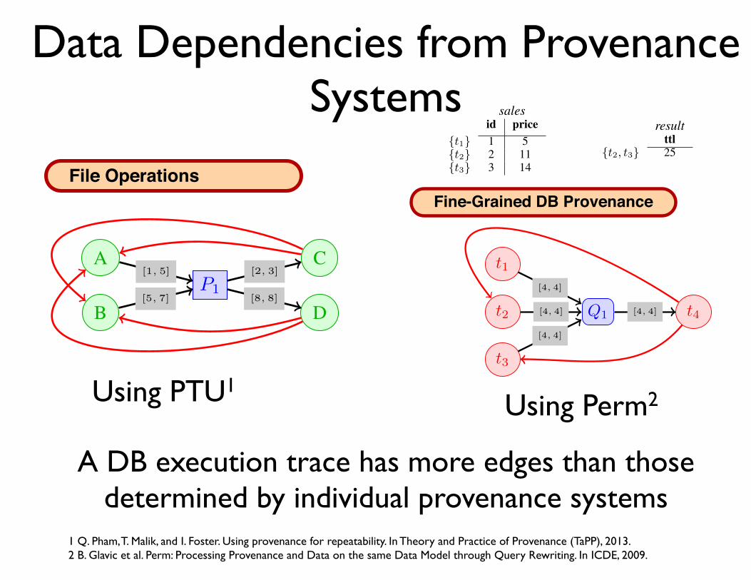
A DB execution trace has more edges than those determined by individual provenance systems

A combined execution trace models the execution of a DBapplication including its processes, file operations, and DBaccesses based on a OS and a DB provenance model.

Definition 6 (Combined Execution Trace). Let PDB and POS

be DB and OS provenance models. Every execution trace forPDB+OS is a combined execution trace for PDB and POS .

Example 3. A combined execution trace for the PLin andPBB models is shown in Figure 2. This trace models theexecution of two processes P1 and P2. Process P1 reads twofiles A and B, and executes two insert statements (at time 5and 8 respectively). These insert statements create three tupleversions t1, t2, and t3. Process P2 executes a query whichreturns tuples t4 and t5. These tuples depend on tuples t1 andt3. Finally, process P2 writes file C.

VI. DATA DEPENDENCIES

The above definitions describe interactions of activities andentities in an execution trace of a provenance model, but do notmodel data dependencies, i.e., dependencies between entities.In our model, a dependency is an edge between two entities e

and e

0 where a change to the input node (e0) may result in achange to the output node (e). Given a provenance model, de-pendency information may or may not be explicitly available;it depends upon the granularity at which information aboutentities and activities is tracked and stored. For instance, theblackbox provenance model PBB operates at the granularityof processes and files and may not compute exact dependencyinformation. Consider a process P that reads from files A andB and writes a file C. File B may be a configuration filethat determines whether the process P logs debug output—anoption that has no effect on the content of file C. A PBB

execution trace cannot not inform about the absence of thisdependency and thus we have to assume that each outputdepends on all inputs. On the contrary, a fine-grained DBprovenance model such as PLin exactly determines the inputtuples on which a query result tuple depends. We now formallystate and explain dependency tracking in these models. Bydefining model-specific dependencies and temporal constraintswe subsequently show how to exclude spurious dependenciesand to infer additional dependencies.

A. Lineage DB Dependencies

We use the Lineage provenance model for DB queriesto determine dependencies between input and output tuplesof DB operations in the PLin model. This model [5], [15]represents the provenance of a query result tuple t as the setof tuples from the DB instance that were used to derive t.This set can be derived from provenance polynomial of tuplet according to the semirings annotation framework [15]. In thesemiring framework, tuples are annotated with elements froma commutative semiring which represent their provenance.Lineage is less informative than provenance polynomials,but is simpler and sufficient for our use case: determiningdependency edges between tuples. Systems such as Perm [10]

salesid price

{t1} 1 5{t2} 2 11{t3} 3 14

resultttl

{t2, t3} 25

Fig. 5: Annotated relation sales and query result

compute provenance polynomials (and thus also Lineage) on-demand for an input query. In the following we will useLin(Q, t) to denote the Lineage of a tuple t in the result of aquery Q.

Example 4. Consider the sales table shown in Fig-ure 5. The Lineage of each tuple in the sales ta-ble is a singleton set containing the tuple’s identi-fier. The result of a query SELECT sum(value) AS ttlFROM sales WHERE price > 10 is a single row with ttl =11+14 = 25. The Lineage contains all tuples (t2 and t3) thatwere used to compute this results.

We define data dependencies in the PLin model based onLineage. We connect each tuple t in the result of a query Q toall input tuples of the query that are in t’s Lineage. Similarly,we connect a modified tuple t in the result of an update to thecorresponding tuple t

0 in the input of the update.

Definition 7 (PLin Data Dependencies). Let G be a PLin

trace. Let Lin(s, t) denote the Lineage of tuple t in the resultof DB operation s, and let t and t

0 denote entities (tuples).The dependencies D(G) ⇢ D ⇥D of G are defined as:

D(G) ={(t, t0) | 9s : (t0, s) 2 E ^ (s, t) 2 E ^ t

0 2 Lin(s, t)}

Example 5. Consider the trace shown in Figure 3 where Q1

is the query from Example 4. Tuple t4 depends on t2 and t3,because these tuples are in the Lineage of t4 according to Q1.

B. Blackbox Process OS Dependencies

As mentioned before, the applications that we track canmaintain arbitrary internal state. Without static program anal-ysis or dynamic instrumentation [26], [24] it is impossible toknow which outputs depend on which inputs. Thus, we mustassume (conservatively) that a file f depends on another filef

0 if there exists a process that reads from file f

0 and writesfile f . Recall that in the PBB model a process may execute achild process. Thus, file f also depends on f

0 if it is connectedto f

0 through a path of process nodes.

Definition 8 (PBB Data Dependencies). Let G be an PBB

trace, f and f

0 be entity (file) nodes in G, and Pi be a processnode. The data dependencies D(G) of G are defined as:

D(G) = {(f, f 0) | 9P1, . . . , Pn : (f 0, P1) 2 E ^ (Pn, f) 2 E

^ 8i 2 {2, . . . , n} : (Pi�1, Pi) 2 E}

The above definition states that there exists a data depen-dency between files f and f

0 if these two files are connectedin the execution trace through a path of processes Pi in which

Using PTU1Using Perm2

1 Q. Pham, T. Malik, and I. Foster. Using provenance for repeatability. In Theory and Practice of Provenance (TaPP), 2013. 2 B. Glavic et al. Perm: Processing Provenance and Data on the same Data Model through Query Rewriting. In ICDE, 2009.

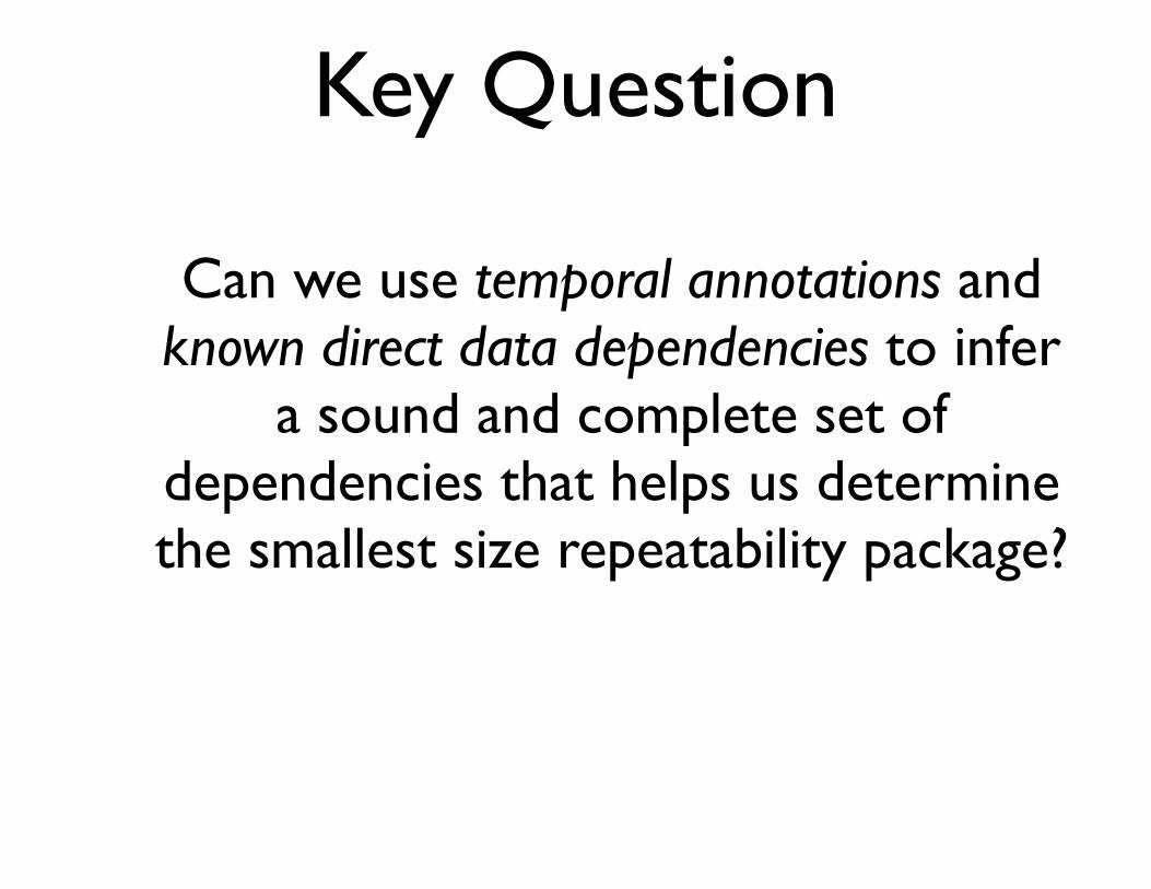
Can we use temporal annotations and known direct data dependencies to infer

a sound and complete set of dependencies that helps us determine the smallest size repeatability package?

Key Question

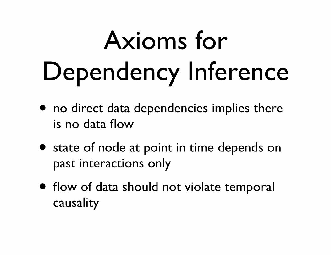
Axioms for Dependency Inference• no direct data dependencies implies there

is no data flow

• state of node at point in time depends on past interactions only

• flow of data should not violate temporal causality

Inferring Dependencies

G. The state S(v, T ) of node v at a time T is defined as:

S(v, T ) = {v0 | (v0, v) 2 E ^ T (v0, v)b T}

The state of a node can be used to infer dependenciesbetween entities based on the temporal annotations on inter-actions in the execution trace which full the conditions ofDefinition 9. The state of an entity e depends on an entitye

0 at a time T if 1) there is a path between e

0 and e in theexecution trace, 2) adjacent entities from the same provenancemodel on this path are connected through data dependencies,and 3) the temporal annotations on the edges of the path donot violate temporal causality.

Example 7. In the execution trace shown in Figure 4, thereexists a path between file B and file C (B ! P1 ! C).However, we cannot infer that C depends on B, because fileC was written ([2, 3]) by P1 before it has read file B.

Definition 11 (Dependency Inference). Let G be an combinedtrace for provenance models POS and PDB . The data depen-dencies of an entity e 2 G at time T include all entities e

0

such there exists a path v1, . . . , vn in the execution trace withv1 = e

0 and vn = e that fulfills the conditions stated below. Lete1, . . . , em denote all entities on this path (where e1 = v1 = e

0

and em = vn = e). We use D

⇤(G) to denote the set of allsuch dependencies.

1) For all i 2 {2,m}, if ei and ei�1 are from the sameprovenance model, then (ei, ei�1) in D(G).

2) There exists a sequence of times T1, . . . , Tn so that foreach i 2 {1,m � 1} we have Ti Ti+1 and Ti T (vi, vi+1)e.

3) For all i 2 {2, n}, the node vi�1 is in the state of vi attime Ti: vi�1 2 S(vi, Ti).

Given assumption 2) an entity e can only depend on entity e

0

if they are connected in the execution trace. Also all adjacententities on such a path should be directly data dependenton each other if they belong to the same provenance model(the 1st assumption enforced by condition 1 of the definitionabove). This guarantees that we do not introduce dependenciesthat do not hold based on the individual provenance models.Conditions 2) and 3) make sure that a dependency does notviolate temporal causality, i.e., the information flow from e

0

to e complies with the temporal annotations.

Theorem 1 (Inference is Sound and Complete). The inferencerules of Definition 11 are sound and complete with respect todependencies that fulfill the assumptions of Definition 9.

Proof: Let Dall(G) denote the set of all dependenciesbetween nodes in G and that are conformant with the threeassumptions we have stated. Furthermore, recall that D⇤(G)denotes the set of dependencies inferred using Definition 11.We have to prove Dall(G) ✓ D

⇤(G), i.e., the rules arecomplete and D

⇤(G) ✓ Dall(G), i.e., the rules are sound.Dall(G) ✓ D

⇤(G): Let (e, e0) 2 Dall(G), i.e., (e, e0) is adependency that fulfills assumptions 1 to 3. We have to showthat (e, e0) 2 D

⇤(G). There have to exist one or more paths

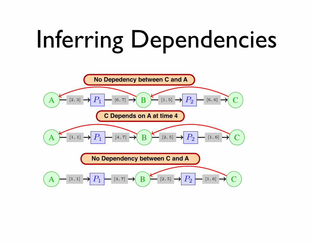
(a) No Dependency between C and A

A P1 B P2 C[2, 3] [6, 7] [1, 5] [6, 6]

(b) C depends on A at time 4

A P1 B P2 C[1, 1] [4, 7] [2, 5] [1, 6]

(c) No Dependency between C and A

A P1 B P2 C[1, 1] [4, 7] [2, 5] [1, 6]

Fig. 6: Example traces with different temporal annotations

between e

0 and e, because if there is no path between e

0 ande in the trace then this would directly violate assumption 2.If conditions 1-3 of Definition 11 hold for one of these paths,then e 2 D

⇤(G). We will now incrementally construct such apath. Given that (e, e0) is a dependency that fulfills the threeassumptions we know that there exists an entity node e

00 sothat the state of e at a time t contains e00 and the state of e00 attime t contains e

0. Otherwise, the dependency would violatetemporal causality and/or assumption 2. WLOG let there beno other entity on the path between e

00 and e that caused e

00

to be in the state (according to Definition 10), i.e., e00 is the“closest” entity to e on this path. Let v1 = e

00, . . . , vn = e be

this path. Based on assumption 3 we can infer that condition3 of Definition 11 holds for this path. Based on the definitionof state (Definition 10) it follows that condition 2 holds too.Finally, if e and e

00 are from the same model, then (e, e00)has to be a dependency in this model based on assumption 1which means condition 1 of Definition 11 holds. Thus, (e00, e)is a dependency in D

⇤(G). Now the same argument can beapplied to find a e

000 between e

0 and e

00. By induction we canconstruct the needed path between (e0, e) and it follows that(e0, e) is in D

⇤(G).D

⇤(G) ✓ Dall(G): Let (e, e0) 2 D

⇤(G). Then we have toprove that (e, e0) 2 Dall(G). In other words, (e, e0) does notviolate any of the three assumptions (and, thus, would be inDall(G)). This is obviously the case, because e

0 and e areconnected through a chain of data dependencies, are connectedin the execution trace, and temporal causality is not violated.

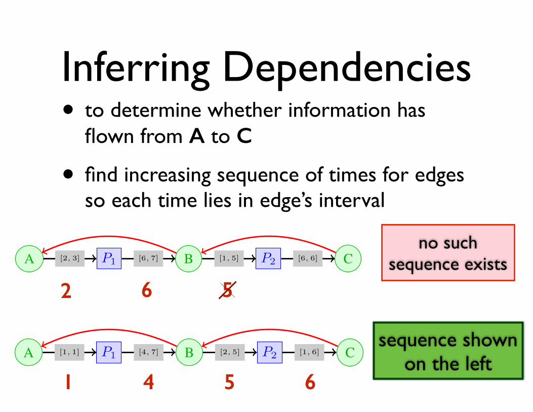
Example 8 (Indirect Data Dependencies). Figure 6 showsseveral versions of the same execution trace with differentdata dependencies and temporal annotations. In trace 6a thereexists a path between A and C and the entities on that pathare connected through data dependencies. However, given thetemporal constraints, C cannot depend on A, because P2

stopped reading B before it was written by P1. No matterwhat time sequence T1, . . . , T5 is chosen, the third conditionof the definition will fail for vi = B. Trace 6b has differenttime annotations and in this trace C depends on A at time 4.For trace 6c there is no data dependency between B and A.


S(v, T ) = {v0 | (v0, v) 2 E ^ T (v0, v)b T}






0



0







0


0









A P1 B P2 C[2, 3] [6, 7] [1, 5] [6, 6]


A P1 B P2 C[1, 1] [4, 7] [2, 5] [1, 6]


A P1 B P2 C[1, 1] [4, 7] [2, 5] [1, 6]


between e







00


00, . . . , vn = e be




000 between e

0 and e


⇤(G).D

⇤(G) ✓ Dall(G): Let (e, e0) 2 D





1 4 5 6

2 6 5

no such sequence exists

• to determine whether information has flown from A to C

• find increasing sequence of times for edges so each time lies in edge’s interval

sequence shown on the left

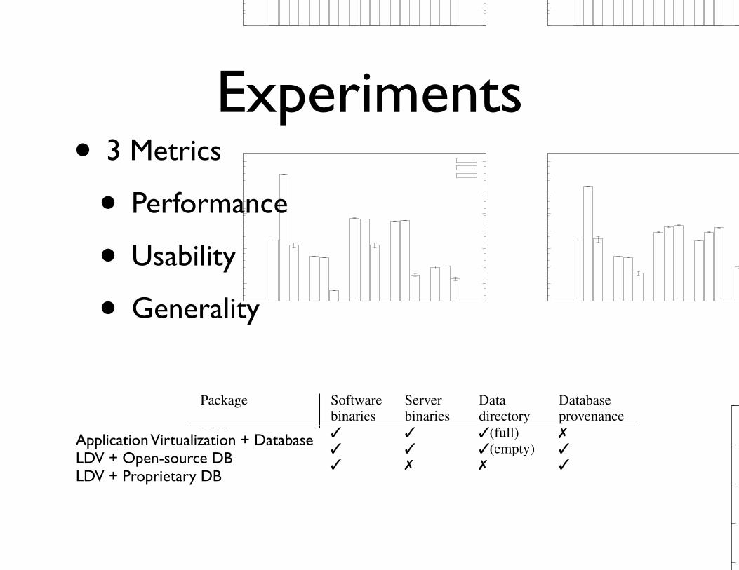
Experiments• 3 Metrics

• Performance

• Usability

• Generality

(a) Q1

1e-05

0.0001

0.001

0.01

0.1

1

10

100

1000

Test Prepare

Inserts FirstSelect

OtherSelects

Updates

Exec

utio

n tim

e (s

econ

ds)

PostgreSQL

0.03

0.00

357

0.56

2

0.37

53

0.00

084

Open-Source DB Server scenario

39.4

0.00

4536

59.2

4

3.17

9

0.00

312

Proprietary DB Server scenario

0.13

6

0.00

5608

1.60

6

0.55

78

0.00

168

(b) Q2

1e-05

0.0001

0.001

0.01

0.1

1

10

100

1000

Test Prepare

Inserts FirstSelect

OtherSelects

Updates

Exec

utio

n tim

e (s

econ

ds)

PostgreSQL

0.03

0.00

348 0.

088

0.02

872

0.00

088


39.4

0.00

4292

2.72

8

0.16

72

0.00

324


0.13

2

0.00

5248

0.50

6

0.41

21

0.00

172

(c) Q3

1e-05

0.0001

0.001

0.01

0.1

1

10

100

1000

Test Prepare

Inserts FirstSelect

OtherSelects

Updates

Exec

utio

n tim

e (s

econ

ds)

PostgreSQL

0.03

0.00

3426

0.19

6

0.01

552

0.00

07


39.4

0.00

428

1.72

8

0.46

57

0.00

302


0.13

4

0.00

536 0.

214

0.01

79

0.00

17

Fig. 7: Execution time of each step in an execution of TPC-H benchmark application in Audit mode

(a) Q1

1e-05

0.0001

0.001

0.01

0.1

1

10

100

1000

Test Prepare

Inserts FirstSelect

OtherSelects

Updates

Exec

utio

n tim

e (s

econ

ds)

PostgreSQL

0.03

0.00

357

0.56

2

0.37

53

0.00

084

Open-Source DB Server scenario178.

2

0.00

3042

0.49

2

0.39

21

0.00

1


0.01

6

4E-0

5

0.01

6

0.00

03

0.00

018

(b) Q2

1e-05

0.0001

0.001

0.01

0.1

1

10

100

1000

Test Prepare

Inserts FirstSelect

OtherSelects

Updates

Exec

utio

n tim

e (s

econ

ds)

PostgreSQL

0.03

0.00

348 0.

088

0.02

872

0.00

088


34.0

9

0.00

3072

0.18

0.08

532

0.00

12


0.03

6

0.00

0376

0.21

8

0.15

55

0.00

042

(c) Q3

1e-05

0.0001

0.001

0.01

0.1

1

10

100

1000

Test Prepare

Inserts FirstSelect

OtherSelects

Updates

Exec

utio

n tim

e (s

econ

ds)

PostgreSQL

0.03

0.00

3426

0.19

6

0.01

552

0.00

07


1.85

2

0.00

3474 0.

086

0.00

284

0.00

12


0.01

6

4E-0

5

0.01

4

0.00

028

0.00

018

Fig. 8: Re-Execution time of each step in an execution of TPC-H benchmark application in Replay mode

Package Softwarebinaries

Serverbinaries

Datadirectory

Databaseprovenance

PTU 3 3 3(full) 7Open-Source DBS 3 3 3(empty) 3Proprietary DBS 3 7 7 3

TABLE III: Content of PTU and LDV packages: PTU pack-ages contain data directory of the full database, whereas Open-Source DBS LDV packages contain a data directory of anempty database (created by the initdb command)

2) Performance in Re-Execution: Figure 8 compares thereplay performance of LDV software packages in Open-SourceDBS and Proprietary DBS scenarios and a normal execution.Open-Source DBS scenario exhibits a long database prepara-tion since LDV needs to restore database state using auditedprovenance. Once the database is restored, performance ofOpen-Source DBS scenario is the same as in the normaluninstrumented execution. It is noticeable that in almost allexperiment steps, Proprietary DBS scenario shows a lowerexecution time than Open-Source DBS scenario and normalexecution. This can be explained as Proprietary DBS appli-cation does not wait for database server to process queries,but read their results directly from local disks. An exceptionappears in the Proprietary DBS scenario with select queries forthe query Q2 where large-size results were returned. In normaland Open-Source DBS scenarios, the cache from databaseserver returned results faster than repeatedly reading resultsfrom disks in Proprietary DBS scenario.

0

100

200

300

400

500

Query #1 Query #2 Query #3

Tota

l pac

kage

siz

e (M

B)

TPC-H Query

Full Capture

100%

100%

100%


71.7

%

55.9

%

54.1

%


16.1

%

324.

3%

16.2

%

Fig. 9: Sizes of packages compared with a full capture

3) Package Size: To explore the improvement of LDVpackages over repeatable software packages that contain fulldatabase, we compare the sizes of LDV and PTU packages toshow a remarkably smaller size packages of LDV approach.A PTU package contains all the necessary binaries, librariesand files required to re-execute the application. This packagecontains all files accessed by the database server in theapplication execution. An LDV package contains databaseprovenance for re-execution, and the database server binariesand a data directory of an empty database in the Open-SourceDBS scenario (Table III).

Using the application with TPC-H query Q1, Q2, and Q3,we constructed their corresponding PTU and Open-SourceDBS, and Proprietary DBS LDV packages. Figure 9 shows

Application Virtualization + DatabaseLDV + Open-source DBLDV + Proprietary DB

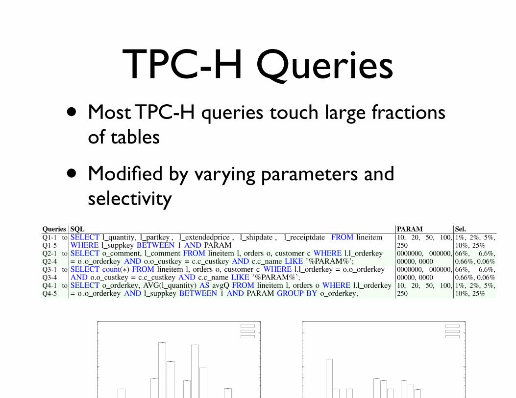
TPC-H Queries• Most TPC-H queries touch large fractions

of tables

• Modified by varying parameters and selectivity

TABLE II: The 18 TPC-H benchmark queries used in our experiments

Queries SQL PARAM Sel.Q1-1 toQ1-5

SELECT l quantity, l partkey , l extendedprice , l shipdate , l receiptdate FROM lineitemWHERE l suppkey BETWEEN 1 AND PARAM

10, 20, 50, 100,250

1%, 2%, 5%,10%, 25%

Q2-1 toQ2-4

SELECT o comment, l comment FROM lineitem l, orders o, customer c WHERE l.l orderkey= o.o orderkey AND o.o custkey = c.c custkey AND c.c name LIKE ’%PARAM%’;

0000000, 000000,00000, 0000

66%, 6.6%,0.66%, 0.06%

Q3-1 toQ3-4

SELECT count(⇤) FROM lineitem l, orders o, customer c WHERE l.l orderkey = o.o orderkeyAND o.o custkey = c.c custkey AND c.c name LIKE ’%PARAM%’;

0000000, 000000,00000, 0000

66%, 6.6%,0.66%, 0.06%

Q4-1 toQ4-5

SELECT o orderkey, AVG(l quantity) AS avgQ FROM lineitem l, orders o WHERE l.l orderkey= o.o orderkey AND l suppkey BETWEEN 1 AND PARAM GROUP BY o orderkey;

10, 20, 50, 100,250

1%, 2%, 5%,10%, 25%

(a) Audit

1e-05

0.0001

0.001

0.01

0.1

1

10

100

1000

10000

Inserts FirstSelect

OtherSelects

Updates

Exec

utio

n tim

e (s

econ

ds)

PostgreSQL + PTUServer-included packageServer-excluded package

(b) Replay

1e-05

0.0001

0.001

0.01

0.1

1

10

100

1000

10000

Initialization Inserts FirstSelect

OtherSelects

Updates

Exec

utio

n tim

e (s

econ

ds)

PostgreSQL + PTU1E

-05

0.01

001

0.08

0.05

3

0.00

01

Server-included package4.

19

0.00

063

0.05

0.02

5

0.00

03

Server-excluded package0.

01

2E-0

5

0.01

0.00

9

0.00

01Fig. 7: Execution time of each step in an application with query Q1-1

(a) Audit

0.001

0.01

0.1

1

10

100

1000

10000

1-1 1-2 1-3 1-4 1-5 2-1 2-2 2-3 2-4 3-1 3-2 3-3 3-4 4-1 4-2 4-3 4-4 4-5

Exec

utio

n tim

e (s

econ

ds)

Query


(b) Replay

0.001

0.01

0.1

1

10

100

1-1 1-2 1-3 1-4 1-5 2-1 2-2 2-3 2-4 3-1 3-2 3-3 3-4 4-1 4-2 4-3 4-4 4-5

Exec

utio

n tim

e (s

econ

ds)

Query


VM

Fig. 8: Execution time for each query, during audit (left) and replay (right)

TABLE III: Package Contents: PTU packages contain all datafiles of the full DB, whereas server-included LDV packagescontain the data files of an empty DB.

Package type Softwarebinaries

DBserver

Datafiles

DBprovenance

PTU 3 3 3(full) 7LDV server-included 3 3 3(empty) 3LDV server-excluded 3 7 7 3

server in the application execution, i.e., the server binaries anddata files. An LDV package contains DB provenance for re-execution, the DB server binaries, and an empty data directoryin the server-included scenario (Table III).

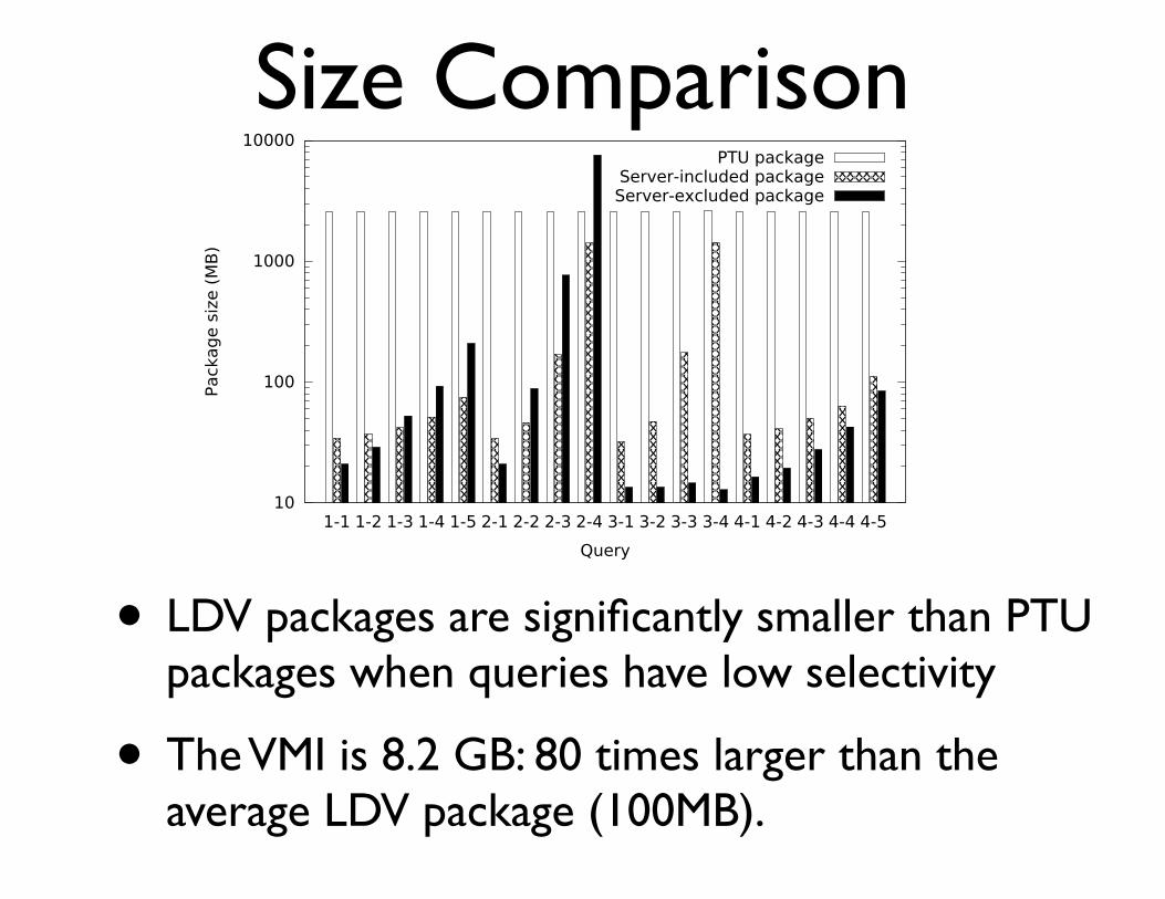
Figure 9 shows the sizes of the PTU, server-included, andserver-excluded packages constructed for the queries listedin Table II. Server-included LDV packages are significantlysmaller than PTU packages, because they contain only those

tuples needed to re-execute the application—which, for thesequeries, is at most ⇠25% of all tuples. Server-excluded LDVpackages are often yet smaller, because they contain only thequery results—which, for many of our experiment queries, aresmaller than the tuples required for re-execution. However,recall that server-excluded packages have less flexibility thando server-included packages.

F. Comparison with the Virtual Machine Approach

We compare a virtual machine image (VMI) with the server-included and server-excluded LDV approaches. The VMI iscreated based on a bare-bone Debian Wheezy 64bit VMI onwhich we install the DB server and the experiment binaries asin Section IX-A. We use “apt-get” to install a DB server, and“scp” to copy all DB files and source code for the experimentfrom our machine. Using the created VMI, we run the sameapplication to compare the size and performance of this VMI

Size Comparison

10

100

1000

10000

1-1 1-2 1-3 1-4 1-5 2-1 2-2 2-3 2-4 3-1 3-2 3-3 3-4 4-1 4-2 4-3 4-4 4-5

Pack

age

size

(MB)

Query

PTU packageServer-included packageServer-excluded package

Fig. 9: LDV packages are significantly smaller than PTUpackages when queries have low selectivity.

and the LDV packages. The VMI is 8.2 GB: 80 times largerthan the average LDV package (100MB). To evaluate runtimeperformance, we instantiate this VMI using the same numberof cores and memory as in our machine to execute our queries.Recall that Figure 8b shows that re-executing these queriesin a VM is slightly slower than a non-audited PostgreSQLexecution, and significantly slower than LDV packages.

X. CONCLUSIONS

We introduced a light-weight DB virtualization (LDV)system that can permit sharing and re-execution of appli-cations that perform DB operations. This system uses datacollected via application monitoring to create re-executablepackages that include an application, its dependencies (datafiles, relevant DB tuples), and a combined execution trace.Such packages can be used to repeat an application or part ofan application in a different environment.

Our LDV framework features an innovative integration ofdistinct OS and DB provenance models, and new methodsfor inferring data dependencies that cross model boundaries.The resulting system creates execution traces according to thisframework and uses these traces to determine which data needsto be included in a repeatability package. It leaves to the userthe choice of whether the package should include the DBMS.Our prototype implementation integrates the PTU (OS) andPerm (DB) provenance systems. In future work, we plan tointegrate with the DB-independent GProM [2] middleware.

XI. ACKNOWLEDGEMENTS

This material is based upon work supported by the NationalScience Foundation under Grants ICER-1343816 and SES-0951576,and by the US Department of Energy under contract DE-AC02-06CH11357. Any opinions, findings, and conclusions or recommen-dations expressed in this material are those of the authors and do notnecessarily reflect the views of the National Science Foundation.

REFERENCES

[1] Y. Amsterdamer et al. Putting Lipstick on Pig: Enabling Database-styleWorkflow Provenance. PVLDB, 5(4), 2011.

[2] B. Arab, B. Glavic, et al. A generic provenance middleware for databasequeries, updates, and transactions. In Proceedings of TaPP, 2014.

[3] N. Balakrishnan, T. Bytheway, et al. Opus: A lightweight system forobservational provenance in user space. In TaPP, 2013.

[4] C. T. Brown. Some myths of reproducible computational research. http://ivory.idyll.org/blog/2014-myths-of-computational-reproducibility.html.

[5] J. Cheney et al. Provenance in Databases: Why, How, and Where.Foundations and Trends in Databases, 1(4), 2009.

[6] F. Chirigati and J. Freire. Towards integrating workflow and databaseprovenance. In Provenance and Annotation of Data and Processes. 2012.

[7] F. S. Chirigati, D. Shasha, and J. Freire. Reprozip: Using provenanceto support computational reproducibility. In TaPP, 2013.

[8] S. C. Dey, S. Riddle, and B. Ludascher. Provenance analyzer: Exploringprovenance semantics with logic rules. In TaPP, 2013.

[9] J. Freire and C. T. Silva. Making computations and publicationsreproducible with vistrails. Computing in Science and Engineering,14(4), 2012.

[10] B. Glavic et al. Perm: Processing Provenance and Data on the sameData Model through Query Rewriting. In ICDE, 2009.

[11] B. Glavic et al. Using sql for efficient generation and querying ofprovenance information. In In search of elegance in the theory andpractice of computation: a Festschrift in honour of Peter Buneman. 2013.

[12] C. A. Goble and D. C. De Roure. myExperiment: social networkingfor workflow-using e-scientists. In Proceedings of the 2Nd Workshopon Workflows in Support of Large-scale Science, 2007.

[13] P. J. Guo et al. CDE: using system call interposition to automaticallycreate portable software packages. In USENIX Annual TechnicalConference, Portland, OR, 2011.

[14] B. Howe. Virtual appliances, cloud computing, and reproducibleresearch. Computing in Science & Engineering, 14(4):36–41, 2012.

[15] G. Karvounarakis and T. Green. Semiring-annotated data: Queries andprovenance. SIGMOD Record, 41(3):5–14, 2012.

[16] K. Keahey et al. Virtual workspaces for scientific applications. Journalof Physics: Conference Series, 78(1), 2007.

[17] N. Kwasnikowska, L. Moreau, and J. Van den Bussche. A formalaccount of the open provenance model. journal, 2010.

[18] S. Lampoudi. The path to virtual machine images as first classprovenance. Age, 2011.

[19] T. Malik, L. Nistor, and A. Gehani. Tracking and sketching distributeddata provenance. In International Conference on eScience, 2010.

[20] L. Moreau and P. Missier. Prov-dm: The prov data model.http://www.w3.org/TR/2013/REC-prov-dm-20130430/, 2013.

[21] K.-K. Muniswamy-Reddy, U. Braun, D. A. Holland, P. Macko,D. Maclean, D. W. Margo, M. I. Seltzer, and R. Smogor. Layeringin provenance systems., 2009.

[22] Q. Pham, T. Malik, and I. Foster. Using provenance for repeatability.In TaPP, 2013.

[23] Q. Pham, T. Malik, and I. Foster. Auditing and maintaining provenancein software packages. In IPAW, 2014.

[24] M. Stamatogiannakis et al. Looking inside the black-box: Capturingdata provenance using dynamic instrumentation. In TAPP, 2014.

[25] Transaction Processing Performance Council. TPC-H benchmark spec-ification. Published at http://www.tcp.org/hspec.html, 2008.

[26] M. Zhang et al. Tracing Lineage beyond Relational Operators. In VLDB,2007.

• LDV packages are significantly smaller than PTU packages when queries have low selectivity

• The VMI is 8.2 GB: 80 times larger than the average LDV package (100MB).

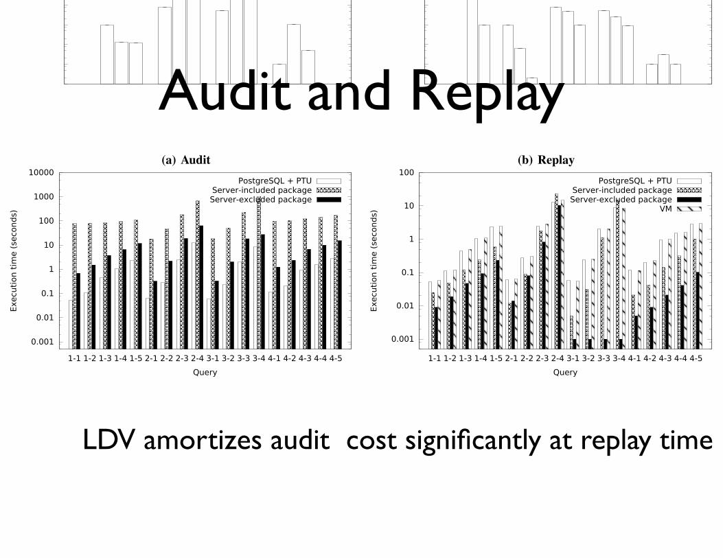
Audit and Replay

TABLE II: The 18 TPC-H benchmark queries used in our experiments

Queries SQL PARAM Sel.Q1-1 toQ1-5

SELECT l quantity, l partkey , l extendedprice , l shipdate , l receiptdate FROM lineitemWHERE l suppkey BETWEEN 1 AND PARAM

10, 20, 50, 100,250

1%, 2%, 5%,10%, 25%

Q2-1 toQ2-4

SELECT o comment, l comment FROM lineitem l, orders o, customer c WHERE l.l orderkey= o.o orderkey AND o.o custkey = c.c custkey AND c.c name LIKE ’%PARAM%’;

0000000, 000000,00000, 0000

66%, 6.6%,0.66%, 0.06%

Q3-1 toQ3-4

SELECT count(⇤) FROM lineitem l, orders o, customer c WHERE l.l orderkey = o.o orderkeyAND o.o custkey = c.c custkey AND c.c name LIKE ’%PARAM%’;

0000000, 000000,00000, 0000

66%, 6.6%,0.66%, 0.06%

Q4-1 toQ4-5

SELECT o orderkey, AVG(l quantity) AS avgQ FROM lineitem l, orders o WHERE l.l orderkey= o.o orderkey AND l suppkey BETWEEN 1 AND PARAM GROUP BY o orderkey;

10, 20, 50, 100,250

1%, 2%, 5%,10%, 25%

(a) Audit

1e-05

0.0001

0.001

0.01

0.1

1

10

100

1000

10000

Inserts FirstSelect

OtherSelects

Updates

Exec

utio

n tim

e (s

econ

ds)


(b) Replay

1e-05

0.0001

0.001

0.01

0.1

1

10

100

1000

10000

Initialization Inserts FirstSelect

OtherSelects

Updates

Exec

utio

n tim

e (s

econ

ds)

PostgreSQL + PTU

1E-0

5

0.01

001

0.08

0.05

3

0.00

01

Server-included package

4.19

0.00

063

0.05

0.02

5

0.00

03

Server-excluded package

0.01

2E-0

5

0.01

0.00

9

0.00

01

Fig. 7: Execution time of each step in an application with query Q1-1

(a) Audit

0.001

0.01

0.1

1

10

100

1000

10000

1-1 1-2 1-3 1-4 1-5 2-1 2-2 2-3 2-4 3-1 3-2 3-3 3-4 4-1 4-2 4-3 4-4 4-5

Exec

utio

n tim

e (s

econ

ds)

Query


(b) Replay

0.001

0.01

0.1

1

10

100

1-1 1-2 1-3 1-4 1-5 2-1 2-2 2-3 2-4 3-1 3-2 3-3 3-4 4-1 4-2 4-3 4-4 4-5Ex

ecut

ion

time

(sec

onds

)Query


VM

Fig. 8: Execution time for each query, during audit (left) and replay (right)

TABLE III: Package Contents: PTU packages contain all datafiles of the full DB, whereas server-included LDV packagescontain the data files of an empty DB.

Package type Softwarebinaries

DBserver

Datafiles

DBprovenance

PTU 3 3 3(full) 7LDV server-included 3 3 3(empty) 3LDV server-excluded 3 7 7 3

server in the application execution, i.e., the server binaries anddata files. An LDV package contains DB provenance for re-execution, the DB server binaries, and an empty data directoryin the server-included scenario (Table III).

Figure 9 shows the sizes of the PTU, server-included, andserver-excluded packages constructed for the queries listedin Table II. Server-included LDV packages are significantlysmaller than PTU packages, because they contain only those

tuples needed to re-execute the application—which, for thesequeries, is at most ⇠25% of all tuples. Server-excluded LDVpackages are often yet smaller, because they contain only thequery results—which, for many of our experiment queries, aresmaller than the tuples required for re-execution. However,recall that server-excluded packages have less flexibility thando server-included packages.

F. Comparison with the Virtual Machine Approach

We compare a virtual machine image (VMI) with the server-included and server-excluded LDV approaches. The VMI iscreated based on a bare-bone Debian Wheezy 64bit VMI onwhich we install the DB server and the experiment binaries asin Section IX-A. We use “apt-get” to install a DB server, and“scp” to copy all DB files and source code for the experimentfrom our machine. Using the created VMI, we run the sameapplication to compare the size and performance of this VMI

LDV amortizes audit cost significantly at replay time

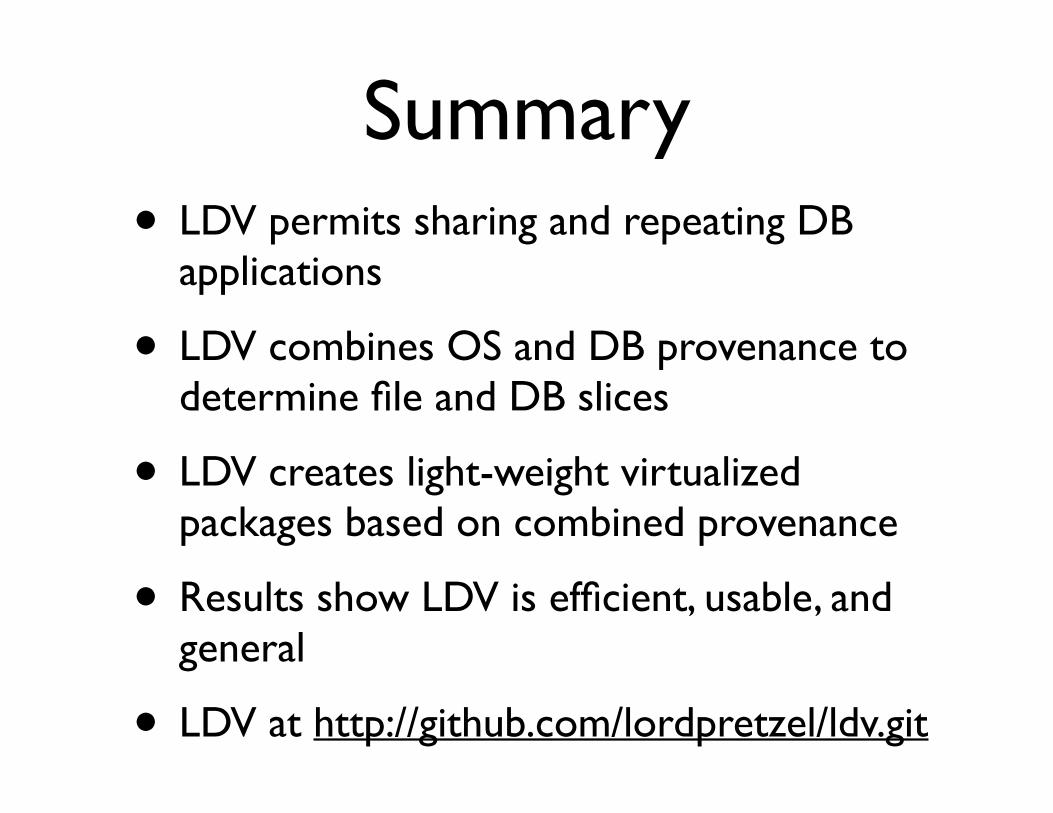
Summary• LDV permits sharing and repeating DB

applications

• LDV combines OS and DB provenance to determine file and DB slices

• LDV creates light-weight virtualized packages based on combined provenance

• Results show LDV is efficient, usable, and general

• LDV at http://github.com/lordpretzel/ldv.git

Q&A

• ?

Inferring DependenciesG. The state S(v, T ) of node v at a time T is defined as:

S(v, T ) = {v0 | (v0, v) 2 E ^ T (v0, v)b T}






0



0







0


0









A P1 B P2 C[2, 3] [6, 7] [1, 5] [6, 6]


A P1 B P2 C[1, 1] [4, 7] [2, 5] [1, 6]


A P1 B P2 C[1, 1] [4, 7] [2, 5] [1, 6]


between e







00


00, . . . , vn = e be




000 between e

0 and e


⇤(G).D

⇤(G) ✓ Dall(G): Let (e, e0) 2 D






S(v, T ) = {v0 | (v0, v) 2 E ^ T (v0, v)b T}






0



0







0


0









A P1 B P2 C[2, 3] [6, 7] [1, 5] [6, 6]


A P1 B P2 C[1, 1] [4, 7] [2, 5] [1, 6]


A P1 B P2 C[1, 1] [4, 7] [2, 5] [1, 6]


between e







00


00, . . . , vn = e be




000 between e

0 and e


⇤(G).D

⇤(G) ✓ Dall(G): Let (e, e0) 2 D






S(v, T ) = {v0 | (v0, v) 2 E ^ T (v0, v)b T}






0



0







0


0









A P1 B P2 C[2, 3] [6, 7] [1, 5] [6, 6]


A P1 B P2 C[1, 1] [4, 7] [2, 5] [1, 6]


A P1 B P2 C[1, 1] [4, 7] [2, 5] [1, 6]


between e







00


00, . . . , vn = e be




000 between e

0 and e


⇤(G).D

⇤(G) ✓ Dall(G): Let (e, e0) 2 D





No Depedency between C and A

C Depends on A at time 4

No Dependency between C and A