Embed Size (px)
DESCRIPTION
AACIMP 2011 Summer School. Operational Research stream. Lecture by Gerhard-Wilhelm Weber.
Citation preview
Portfolio Optimization
Gerhard-Wilhelm Weber1 Erik Kropat2 Zafer-Korcan Görgülü3
1Institute of Applied MathematicsMiddle East Technical University
Ankara, Turkey
2Department of MathematicsUniversity of Erlangen-Nuremberg
Erlangen, Germany
3University of the Federal Armed ForcesMunich, Germany
2008
1 / 477
Outline I
1 The Mean-Variance Approach in a One-Period ModelIntroduction
2 The Continuous-Time Market ModelModeling the Security PricesExcursion 1: Brownian Motion and MartingalesContinuation: Modeling the Security pricesExcursion 2: The Ito IntegralExcursion 3: The Ito FormulaTrading Strategy and Wealth ProcessProperties of the Continuous-Time Market ModelExcursion 4: The Martingale Representation Theorem
2 / 477

Outline II
3 Option PricingIntroductionExamplesThe Replication PrincipleArbitrage OpportunityContinuationPartial Differential Approach (PDA)Arbitrage & Option Pricing
3 / 477

Outline III
4 Pricing of Exotic Options and Numerical AlgorithmsIntroductionExamplesExamplesEquivalent Martingale MeasureExotic Options with Explicit Pricing FormulaeWeak Convergence of Stochastic ProcessesMonte-Carlo SimulationApproximation via Binomial TreesThe Pathwise Binomial Approach of Rogers and Stapleton
4 / 477

Outline IV
5 Optimal PortfoliosIntroduction and Formulation of the ProblemThe martingale methodOptimal Option PortfoliosExcursion 8: Stochastic ControlMaximize expected value in presence of quadratic control costsIntroductionPortfolio Optimization via Stochastic Control Method
5 / 477

Outline
1 The Mean-Variance Approach in a One-Period Model
6 / 477

Outline
1 The Mean-Variance Approach in a One-Period ModelIntroduction
7 / 477

Introduction
MVA Based on H. MARKOWITZ
OPM • Decisions on investment strategies only at the beginning of theperiod
• Consequences of these decisions will be observed at the end of theperiod (−→ no action in between: static model )
8 / 477

The one-period model
Market with d traded securitiesd different securities with positive prices p1, . . . , pd at time t = 0
Security prices P1(T ), . . . , Pd (T ) at final time t = T notforeseeable−→ modeled as non-negative random variables on probability space
(Ω,F ,P)
9 / 477
Securities in a OPM
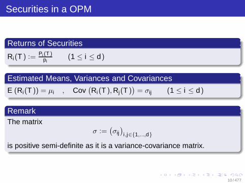
Returns of Securities
Ri(T ) := Pi (T )pi
(1 ≤ i ≤ d)
Estimated Means, Variances and Covariances
E (Ri(T )) = µi , Cov(Ri(T ), Rj(T )
)= σij (1 ≤ i ≤ d)
RemarkThe matrix
σ :=(σij)
i ,j∈1,...,d
is positive semi-definite as it is a variance-covariance matrix.
10 / 477

Securities in a OPM
Each security perfectly divisable
Hold ϕi ∈ R shares of security i (1 ≤ i ≤ d)
Negative position (ϕi < 0 for some i) corresponds to a selling−→ Not allowed in OPM
−→ No negative positions: pi ≥ 0 (1 ≤ i ≤ d)−→ No transaction costs
11 / 477
Budget equation and portfolio return
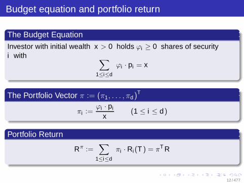
The Budget EquationInvestor with initial wealth x > 0 holds ϕi ≥ 0 shares of securityi with ∑
1≤i≤d
ϕi · pi = x
The Portfolio Vector π := (π1, . . . , πd)T
πi :=ϕi · pi
x(1 ≤ i ≤ d)
Portfolio Return
Rπ :=∑
1≤i≤d
πi · Ri(T ) = πT R
12 / 477

Budget equation and portfolio return
Remarkπi . . . fraction of total wealth invested in security i
∑
1≤i≤d
πi =
∑1≤i≤d
ϕi · pi
x=
xx
= 1
Xπ(T ) . . . final wealth corresponding to x and π
Xπ(T ) =∑
1≤i≤d
ϕi · Pi(T )
13 / 477

Budget equation and portfolio return
Remark (continued)Portfolio Return
Rπ =∑
1≤i≤d
πi · Ri(T ) =∑
1≤i≤d
ϕi · pi
x· Pi(T )
pi=
Xπ(T )
x
Portfolio Mean and Portfolio Variance
E (Rπ) =∑
1≤i≤d
πi · µi , Var (Rπ) =∑
1≤i ,j≤d
πi · σij · πj
14 / 477

Selection of a portfolio–criterion
(i) Maximize mean return (choose security of highest mean return)−→ risky, big fluctuations of return
(ii) Minimize risk of fluction
15 / 477

Selection of a portfolio–approach by Markowitz (MVA)
Balance Risk (Portfolio Variance) and Return (Portfolio Mean)(i) Maximize E (Rπ) under given upper bound c1 for Var (Rπ)
maxπ∈Rd
E (Rπ) subject to
πi ≥ 0 (1 ≤ i ≤ d)∑
1≤i≤d
πi = 1
Var (Rπ) ≤ c1
(ii) Minimize Var (Rπ) under given lower bound c2 for E (Rπ)
minπ∈Rd
Var (Rπ) subject to
πi ≥ 0 (1 ≤ i ≤ d)∑
1≤i≤d
πi = 1
E (Rπ) ≥ c2
16 / 477

Solution methods
(i) Linear Optimization Problem with quadratic constraint−→ No standard algorithms, numerical inefficient
(ii) Quadratic Optimization Problem with positive semidefiniteobjective matrix σ
−→ efficient algorithms (i.e., GOLDFARB/IDNANI, GILL/MURRAY)Feasible region non-empty if c2 ≤ max
1≤i≤dµi
σ positive definite and feasible region non-empty−→ unique solution (even if one security riskless)
17 / 477
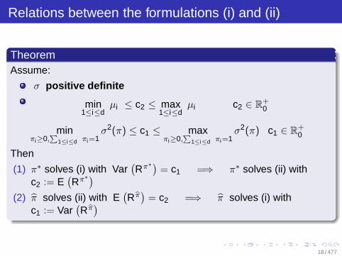
Relations between the formulations (i) and (ii)
TheoremAssume:
σ positive definite
min1≤i≤d
µi ≤ c2 ≤ max1≤i≤d
µi c2 ∈ R+0
minπi≥0,
∑1≤i≤d πi=1
σ2(π) ≤ c1 ≤ maxπi≥0,
∑1≤i≤d πi=1
σ2(π) c1 ∈ R+0
Then
(1) π∗ solves (i) with Var(Rπ∗)
= c1 =⇒ π∗ solves (ii) withc2 := E
(Rπ∗)
(2) π solves (ii) with E(Rπ)
= c2 =⇒ π solves (i) withc1 := Var
(Rπ)
18 / 477
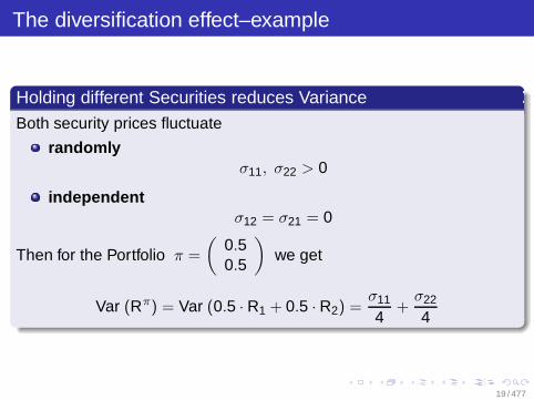
The diversification effect–example
Holding different Securities reduces VarianceBoth security prices fluctuate
randomlyσ11, σ22 > 0
independentσ12 = σ21 = 0
Then for the Portfolio π =
(0.50.5
)we get
Var (Rπ) = Var (0.5 · R1 + 0.5 · R2) =σ11
4+
σ22
4
19 / 477

The diversification effect–example
Holding different Securities reduces Variance
−→ If σ11 = σ22 then the Variance of Portfolio(
0.50.5
)is half as big
as that of(
10
)or(
01
)
−→ Reduction of Variance . . . Diversification Effect depends onnumber of traded securities
20 / 477
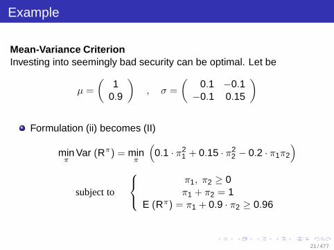
Example
Mean-Variance CriterionInvesting into seemingly bad security can be optimal. Let be
µ =
(1
0.9
), σ =
(0.1 −0.1
−0.1 0.15
)
Formulation (ii) becomes (II)
minπ
Var (Rπ) = minπ
(0.1 · π2
1 + 0.15 · π22 − 0.2 · π1π2
)
subject to
π1, π2 ≥ 0π1 + π2 = 1
E (Rπ) = π1 + 0.9 · π2 ≥ 0.96
21 / 477

Example
Consider Portfolios(
10
)and
(0.50.5
)(does not satify
expectation constraint)
Var(
R(1,0)T)
= 0.1 , E(
R(1,0)T)
= 1
Var(
R(0.5,0.5)T)
= 0.125 , E(
R(0.5,0.5)T)
= 0.95
22 / 477

Example
Ignore expectation constraint and rememberπ1, π2 ≥ 0 π1 + π2 = 1. Hence
minπ
(0.1 · π2
1 + 0.15 · (1 − π1)2 − 0.2 · π1 · (1 − π1)
)
= minπ
(0.45 · π2
1 − 0.5 · π1 + 0.15)
−→ Minimizing Portfolio (No solution of (II) but better than(
0.50.5
))
π =19·(
54
)
−→ Portfolio Return Variance Var(
R( 59 ,
49 )
T)= 0.001
−→ Portfolio Return Mean E(
R( 59 ,
49 )
T)= 0.95
23 / 477

Example
0.0 0.5 0.6 1.00.0
0.4
0.5
1.0
π1
π2
Pairs (π1, π2) satisfying expectation constraint are above thedotted line
Intersect with line π1 + π2 = 1−→ Feasible region of MeanVariance Problem (bold line)
24 / 477
Example
0 0.5 0.6 1.0 1.50
0.05
0.1
0.15
π1
Var
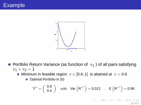
Portfolio Return Variance (as function of π1 ) of all pairs satisfyingπ1 + π2 = 1
Minimum in feasible region π ∈ [0.6, 1] is attained at π = 0.6Optimal Portfolio in (II)
−→π
∗ =
(0.60.4
)with Var
(Rπ∗
)= 0.012 , E
(Rπ∗
)= 0.96
25 / 477
Stock price model
OPMNo assumption on distribution of security returns
Solving MV Problem just needed expectations and covariances
26 / 477

Stock price model
OPM with just one security (price p1 at time t = 0 )At time T security may have price d · p1 or u · p1
q : probability of decreasing by factor d1 − q : probability of increasing by factor u (u > d)
Mean and Variance of Return
E (R1(T )) = E(
P1(T )
p1
)= q · u + (1 − q) · d
Var (R1(T )) = Var(
P1(T )
p1
)= q · u2 + (1 − q) · d2
− (q · u + (1 − q) · d)2
27 / 477

Stock price model
OPM with just one security (price p1 at time t = 0 )After n periods the security has price
P1(n · T ) = p1 · uXn · dn−Xn
with Xn ∼ B(n, p) number of up-movements of price inn periods
28 / 477

Comments on MVA
Only trading at initial time t = 0
No reaction to current price changes possible( −→ static model )
Risk of investment only modeled by variance of return
Need of Continuous-Time Market ModelsDiscrete-time multi-period models(many periods −→ no fast algorithms)
29 / 477

Outline
2 The Continuous-Time Market Model
30 / 477

Outline
2 The Continuous-Time Market ModelModeling the Security PricesExcursion 1: Brownian Motion and MartingalesContinuation: Modeling the Security pricesExcursion 2: The Ito IntegralExcursion 3: The Ito FormulaTrading Strategy and Wealth ProcessProperties of the Continuous-Time Market ModelExcursion 4: The Martingale Representation Theorem
31 / 477

Modeling the security prices
Market with d+1 securitiesd risky stocks withprices p1, p2, . . . , pd at time t = 0 andrandom prices P1(t), P2(t), . . . , Pd (t) at times t > 0
1 bond withprice p0 at time t = 0 anddeterministic price P0(t) at times t > 0.
Assume: Perfectly devisible securities, no transaction costs.
⇒ Modeling of the price development on the time interval [0, T ].
32 / 477
The bond price
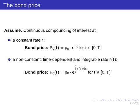
Assume: Continuous compounding of interest at
a constant rate r :
Bond price: P0(t) = p0 · er ·t for t ∈ [0, T ]
a non-constant, time-dependent and integrable rate r(t):
Bond price: P0(t) = p0 · e
t∫
0r(s) ds
for t ∈ [0, T ]
33 / 477
The stock price
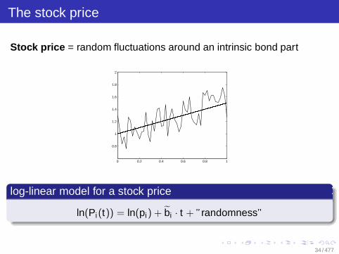
Stock price = random fluctuations around an intrinsic bond part
0 0.2 0.4 0.6 0.8 1
0.8
1
1.2
1.4
1.6
1.8
2
log-linear model for a stock price
ln(Pi(t)) = ln(pi) + bi · t + ”randomness”
34 / 477

The stock price
Randomness is assumed
to have no tendency, i.e., E("randomness") = 0,
to be time-dependent,
to represent the sum of all deviations ofln(Pi(t)) from ln(pi) + bi · t on [0, T ],
∼ N (0, σ2t) for some σ > 0.
35 / 477
The stock price
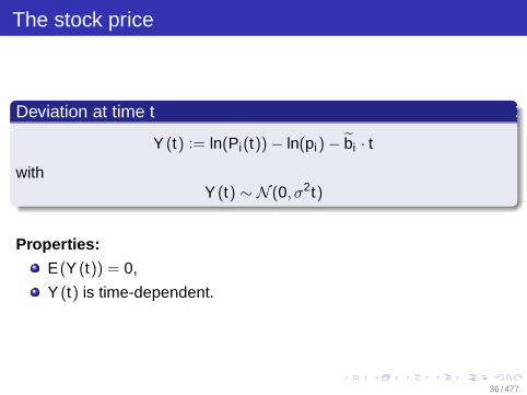
Deviation at time t
Y (t) := ln(Pi(t)) − ln(pi) − bi · t
withY (t) ∼ N (0, σ2t)
Properties:
E(Y (t)) = 0,
Y (t) is time-dependent.
36 / 477

The stock price
Y (t) = Y (δ) + (Y (t) − Y (δ)), δ ∈ (0, t)
Distribution of the increments of the deviation Y (t) − Y (δ)
depends only on the time span t − δ
is independent of Y (s), s ≤ δ
=⇒ Y (t) − Y (δ) ∼ N(0, σ2(t − δ)
)
37 / 477

The stock price
Existence and properties of the stochastic process
Y (t)t∈[0,∞)
will be studied in the excursion on the Brownian motion .
38 / 477

Outline
2 The Continuous-Time Market ModelModeling the Security PricesExcursion 1: Brownian Motion and MartingalesContinuation: Modeling the Security pricesExcursion 2: The Ito IntegralExcursion 3: The Ito FormulaTrading Strategy and Wealth ProcessProperties of the Continuous-Time Market ModelExcursion 4: The Martingale Representation Theorem
39 / 477

General assumptions
General assumptionsLet (Ω,F , P) be a complete probability space with sample space Ω,σ-field F and probability measure P.
40 / 477
Filtration
DefinitionLet Ftt∈I be a family of sub-σ-fields of F , I be an ordered index setwith Fs ⊂ Ft for s < t , s, t ∈ I. The family Ftt∈I is called a filtration.
A filtration describes flow of information over time.
Ft models events observable up to time t .
If a random variable Xt is Ft -measurable, we are able todetermine its value from the information given at time t .
41 / 477
Stochastic process
DefinitionA set (Xt , Ft)t∈I consisting of a filtration Ftt∈I and a family ofR
n-valued random variables Xtt∈I with Xt being Ft -measurable iscalled a stochastic process with filtration Ftt∈I .
42 / 477

Remark
RemarkI = [0,∞) or I = [0, T ].
Canoncial filtration (natural filtration) of Xtt∈I :
Ft := FXt := σXs | s ≤ t , s ∈ I.
Notation: Xtt∈I = X (t)t∈I = X .
43 / 477

Sample path
Sample pathFor fixed ω ∈ Ω the set
X .(ω) := Xt(ω)t∈I = X (t , ω)t∈I
is called a sample path or a realization of the stochastic process.
44 / 477

Identification of stochastic processes
Can two stochastic processes be identified with each other?
DefinitionLet (Xt , Ft)t∈[0,∞) and (Yt , Gt)t∈[0,∞) be two stochastic processes.Y is a modification of X , if
Pω |Xt(ω) = Yt(ω) = 1 for all t ≥ 0.
DefinitionLet (Xt , Ft)t∈[0,∞) and (Yt , Gt)t∈[0,∞) be two stochastic processes.X and Y are indistinguishable, if
Pω |Xt(ω) = Yt(ω) for all t ∈ [0,∞) = 1.
45 / 477

Identification of stochastic processes
RemarkX , Y indistinguishable ⇒ Y modification of X .
TheoremLet the stochastic process Y be a modification of X . If both processeshave continuous sample paths P-almost surely, then X and Y areindistinguishable.
46 / 477

Brownian motion
DefinitionThe real-valued process Wtt≥0 with continuous sample paths and
i) W0 = 0 P-a.s.
ii) Wt − Ws ∼ N (0, t − s) for 0 ≤ s < t"stationary increments"
iii) Wt − Ws independent of Wu − Wr for 0 ≤ r ≤ u ≤ s < t"independent increments"
is called a one-dimensional Brownian motion.
47 / 477

Brownian motion
RemarkBy an n-dimensional Brownian motion we mean the R
n-valued process
W (t) = (W1(t), . . . , Wn(t)),
with components Wi being independent one-dimensional Brownianmotions.
48 / 477

Brownian motion and filtration
Brownian motion can be associated with
natural filtration
FWt := σWs |0 ≤ s ≤ t, t ∈ [0,∞)
P-augmentation of the natural filtration (Brownian filtration)
Ft := σFWt ∪ N |N ∈ F , P(N) = 0, t ∈ [0,∞)
49 / 477

Brownian motion and filtration
Requirement iii) of a Brownian motion with respect to a filtrationFtt≥0 is often stated as
iii)∗ Wt − Ws independent of Fs, 0 ≤ s < t .
Ftt≥0 natural filtration (Brownian filtration)
⇒ iii) and iii)∗ are equivalent.
Ftt≥0 arbitrary filtration
⇒ iii) and iii)∗ are usually not equivalent.
ConventionIf we consider a Brownian motion (Wt ,Ft)t≥0 with an arbitraryfiltration we implicitly assume iii)∗ to be fulfilled.
50 / 477

Existence of the Brownian motion
How can we show the existence of a stochastic process satisfying therequirements of a Brownian motion?
Construction and existence proofs are long and technical.
Construction based on weak convergence and approximation byrandom walks [Billingsley 1968].
Wiener measure, Wiener process.
51 / 477

Brownian motion and filtration
TheoremThe Brownian filtration Ftt≥0 is right-continuous as well asleft-continuous, i.e., we have
Ft = Ft+ :=⋂
ε>0
Ft+ε and Ft = Ft− := σ
(⋃
s<t
Fs
).
DefinitionA filtration Gtt≥0 satifies the usual conditions, if it is right-continuousand G0 contains all P-null sets of F .
General assumption for this sectionLet Ftt≥0 be a filtration which satisfies the usual conditions.
52 / 477

Martingales
DefinitionThe real-valued process (Xt ,Ft)t∈I with E |Xt | < ∞ for all t ∈ I(where I is an ordered index set), is called
a super-martingale, if for all s, t ∈ I with s ≤ t we have
E(Xt |Fs) ≤ Xs P-a.s. ,
a sub-martingale, if for all s, t ∈ I with s ≤ t we have
E(Xt |Fs) ≥ Xs P-a.s. ,
a martingale, if for all s, t ∈ I with s ≤ t we have
E(Xt |Fs) = Xs P-a.s. .
53 / 477

Interpretation of the martingale concept
Example: Modeling games of chance
Xn: Wealth of a gambler after n-th participation in a fair game
Martingale condition: E(Xn+1|Fn) = Xn P-a.s.
⇒ "After the game the player is as rich as he was before"
favorable game = sub-martingalenon-favorable game = super-martingale
54 / 477

Interpretation of the martingale concept
Example: Tossing a fair coin
"Head": Gambler receives one dollar
"Tail": Gambler loses one dollar
⇒ Martingale
55 / 477

Interpretation of the martingale concept
TheoremA one-dimensional Brownian motion Wt is a martingale.
RemarkEach stochastic process with independent, centered increments isa martingale with respect to its natural filtration.
The Brownian motion with drift µ and volatility σ
Xt := µt + σWt , µ ∈ R, σ ∈ R
is a martingale if µ = 0, a super-martingale if µ ≤ 0 and asub-martingale if µ ≥ 0.
56 / 477

Interpretation of the martingale concept
Theorem(1) Let (Xt , Ft)t∈I be a martingale and ϕ : R → R be a convex
function with E |ϕ(Xt)| < ∞ for all t ∈ I. Then
(ϕ(Xt ),Ft)t∈I
is a sub-martingale.
(2) Let (Xt , Ft)t∈I be a sub-martingale and ϕ : R → R a convex,non-decreasing function with E |ϕ(Xt)| < ∞ for all t ∈ I. Then
(ϕ(Xt ),Ft)t∈I
is a sub-martingale.
57 / 477

Interpretation of the martingale concept
Remark(1) Typical applications are given by
ϕ(x) = x2, ϕ(x) = |x |.
(2) The theorem is also valid for d -dimensional vectors
X (t) = (X1(t), . . . , Xd(t))
of martingales and convex functions ϕ : Rd → R.
58 / 477

Stopping time
DefinitionA stopping time with respect to a filtration Ftt∈[0,∞)
(or Fnn∈N) is an F-measurable random variable
τ : Ω → [0,∞] (or τ : Ω → N ∪ ∞)
with ω ∈ Ω | τ(ω) ≤ t ∈ Ft for all t ∈ [0,∞)(or ω ∈ Ω | τ(ω) ≤ n ∈ Fn for all n ∈ N).
TheoremIf τ1, τ2 are both stopping times then τ1 ∧ τ2 := minτ1, τ2 is also astopping time.
59 / 477
The stopped process
The stopped processLet (Xt , Ft)t∈I be a stochastic process, let I be either N or [0,∞),and τ a stopping time. The stopped process Xt∧τt∈I is defined by
Xt∧τ (ω) :=
Xt(ω) if t ≤ τ(ω),
Xτ(ω)(ω) if t > τ(ω).
Example: Wealth of a gambler who participates in a sequence ofgames until he is either bankrupt or has reached a given level ofwealth.
60 / 477

The stopped filtration
The stopped filtrationLet τ be a stopping time with respect to a filtration Ftt∈[0,∞).
σ-field of events determined prior to the stopping time τ
Fτ := A ∈ F |A ∩ τ ≤ t ∈ Ft for all t ∈ [0,∞)
Stopped filtrationFτ∧tt∈[0,∞).
61 / 477

The stopped filtration
What will happen if we stop a martingale or a sub-martingale?
Theorem: Optional sampling
Let (Xt , Ft)t∈[0,∞) be a right-continuous sub-martingale (ormartingale). Let τ1, τ2 be stopping times with τ1 ≤ τ2. Then for allt ∈ [0,∞) we have
E(Xt∧τ2 | Ft∧τ1) ≥ Xt∧τ1 P-a.s.
(orE(Xt∧τ2 | Ft∧τ1) = Xt∧τ1 P-a.s.).
62 / 477

The stopped filtration
CorollaryLet τ be a stopping time and (Xt , Ft)t∈[0,∞) a right-continuoussub-martingale (or martingale). Then the stopped process(Xt∧τ ,Ft)t∈[0,∞) is also a sub-martingale (or martingale).
63 / 477

The stopped filtration
TheoremLet (Xt , Ft)t∈[0,∞) be a right-continuous process. Then Xt is amartingale if and only if for all bounded stopping times τ we have
EXτ = EX0.
→ Characterization of a martingale
64 / 477

The stopped filtration
DefinitionLet (Xt , Ft)t∈[0,∞) be a stochastic process with X0 = 0. If there is anon-decreasing sequence τnn∈N of stopping times with
P(
limn→∞
τn = ∞)
= 1,
such that (X (n)
t := (Xt∧τn ,Ft)
)
t∈[0,∞)
is a martingale for all n ∈ N, then X is a local martingale. Thesequence τnn∈N is called a localizing sequence corresponding to X .
65 / 477

The stopped filtration
Remark(1) Each martingale is a local martingale.
(2) A local martingale with continuous paths is calledcontinuous local martingale.
(3) There exist local martingales which are not martingales.
E(Xt) need not exist for a local martingale. However, theexpectation has to exist along the localizing sequence t ∧ τn.
The local martingale is a martingale on the random timeintervals [0, τn].
TheoremA non-negative local martingale is a super-martingale.
66 / 477

The stopped filtration
Theorem: Doob’s inequalityLet Mtt≥0 be a martingale with right-continuous paths andE(M2
T ) < ∞ or all T > 0. Then, we have
E((
sup0≤t≤T
|Mt |)2)
≤ 4 · E(M2T ).
TheoremLet (Xt , Ft)t∈[0,∞) be a non-negative super-martingale withright-continuous paths. Then, for λ > 0 we obtain
λ · P
ω
∣∣∣∣ sup0≤s≤t
Xs(ω) ≥ λ
≤ E(X0).
67 / 477
Outline
2 The Continuous-Time Market ModelModeling the Security PricesExcursion 1: Brownian Motion and MartingalesContinuation: Modeling the Security pricesExcursion 2: The Ito IntegralExcursion 3: The Ito FormulaTrading Strategy and Wealth ProcessProperties of the Continuous-Time Market ModelExcursion 4: The Martingale Representation Theorem
68 / 477

Continuation: The stock price
log-linear model for a stock price
ln(Pi(t)) = ln(pi) + bi · t + ”randomness”
Brownian motion (Wt , Ft)t≥0 is the appropriate stochastic process tomodel the "randomness"
69 / 477

Continuation: The stock price
Market with one stock and one bond (d=1)
ln(P1(t)) = ln(p1) + b1 · t + σ11Wt
P1(t) = p1 · exp(b1 · t + σ11Wt
)
Market with d stocks and one bond (d>1)
ln(Pi(t)) = ln(pi) + bi · t +
m∑
j=1
σijWj(t), i = 1, . . . , d
Pi(t) = pi · exp(
bi · t +
m∑
j=1
σijWj(t))
, i = 1, . . . , d
70 / 477
Continuation: The stock price
Distribution of the logarithm of the stock prices
ln(Pi(t)) ∼ N(
ln(pi) + bi · t ,m∑
j=1
σ2ij · t)
⇒ Pi(t) is log-normally distributed.
71 / 477

Continuation: The stock price
Lemma
Let bi := bi + 12
m∑
j=1
σ2ij for i = 1, . . . , d.
(1) E(Pi(t)) = pi · ebi t .
(2) Var(Pi(t)) = p2i · exp(2bi t) ·
(exp
( m∑
j=1
σ2ij t)− 1)
.
(3) Xt := a · exp( m∑
j=1
(cjWj(t) −
12
c2j t))
with a, cj ∈ R, j = 1, . . . , m
is a martingale.
72 / 477
Interpretation of the stock price model
The stock price model
Pi(t) = pi · exp(bi t) · exp( m∑
j=1
[σijWj(t) −
12σ2
ij t])
,
Pi(0) = pi , i = 1, . . . , d .
The stock price is the product of
the mean stock price pi · exp(bi t) and
a martingale with expectation 1, namely
exp( m∑
j=1
[σijWj(t) −
12σ2
ij t])
which models the stock price around its mean value.
73 / 477

Interpretation of the stock price model
Vector of mean rates of stock returns
b = (b1, . . . , bd )T
Volatility matrix
σ =
σ11 . . . σ1m...
. . ....
σd1 . . . σdm
Pi(t) is a geometric Brownian motion with drift bi and volatilityσi . = (σi1, . . . , σim)T .
74 / 477
Summary: Stock prices
Bond price and stock prices
P0(t) = p0 · ertBond price
P0(0)= p0
Pi(t) = pi · exp(bi t) · exp( m∑
j=1
[σijWj(t) −
12
σ2ij t])
Stock prices
Pi(0) = pi , i = 1, . . . , d .
75 / 477
Extension
Extension: Model with non-constant, time-dependent, and integrablerates of return bi(t) and volatilities σ(t).
Stock prices:
Pi(t) = pi · exp( t∫
0
(bi(s) − 1
2
m∑
j=1
σ2ij (s)
)ds)
· exp( m∑
j=1
t∫
0
σij(s) dWj(s)
)
Problem:t∫
0σij(s) dWj(s)
⇒ Stochastic integral (Ito integral)
76 / 477
Outline
2 The Continuous-Time Market ModelModeling the Security PricesExcursion 1: Brownian Motion and MartingalesContinuation: Modeling the Security pricesExcursion 2: The Ito IntegralExcursion 3: The Ito FormulaTrading Strategy and Wealth ProcessProperties of the Continuous-Time Market ModelExcursion 4: The Martingale Representation Theorem
77 / 477
The Ito integral
Is it possible to define the stochastic integral
t∫
0
Xs(ω) dWs(ω)
ω-wise in a reasonable way?
78 / 477

The Ito integral
TheoremP-almost all paths of the Brownian motion Wtt∈[0,∞) are nowheredifferentiable.
⇒ A definition of the form
t∫
0
Xs(ω) dWs(ω) =
t∫
0
Xs(ω)dWs(ω)
dsds
is impossible.
79 / 477
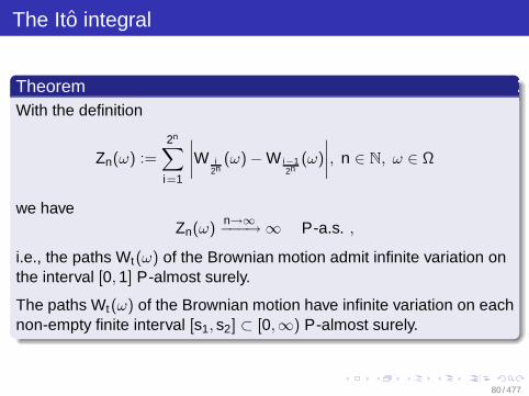
The Ito integral
TheoremWith the definition
Zn(ω) :=
2n∑
i=1
∣∣∣∣W i2n
(ω) − W i−12n
(ω)
∣∣∣∣, n ∈ N, ω ∈ Ω
we haveZn(ω)
n→∞−−−→ ∞ P-a.s. ,
i.e., the paths Wt(ω) of the Brownian motion admit infinite variation onthe interval [0, 1] P-almost surely.
The paths Wt(ω) of the Brownian motion have infinite variation on eachnon-empty finite interval [s1, s2] ⊂ [0,∞) P-almost surely.
80 / 477

General assumptions
General assumptions for this sectionLet (Ω,F , P) be a complete probability space equipped with a filtrationFtt satisfying the usual conditions. Further assume that on thisspace a Brownian motion (Wt ,Ft)t∈[0,∞) with respect to this filtrationis defined.
81 / 477
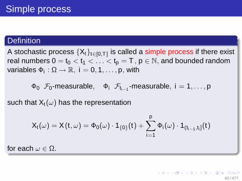
Simple process
DefinitionA stochastic process Xtt∈[0,T ] is called a simple process if there existreal numbers 0 = t0 < t1 < . . . < tp = T , p ∈ N, and bounded randomvariables Φi : Ω → R, i = 0, 1, . . . , p, with
Φ0 F0-measurable, Φi Fti−1 -measurable, i = 1, . . . , p
such that Xt(ω) has the representation
Xt(ω) = X (t , ω) = Φ0(ω) · 10(t) +
p∑
i=1
Φi(ω) · 1(ti−1,ti ](t)
for each ω ∈ Ω.
82 / 477

Simple process
RemarkXt is Fti−1-measurable for all t ∈ (ti−1, ti ].
The paths X (., ω) of the simple process Xt are left-continuous stepfunctions with height Φi(ω) · 1(ti−1,ti ](t).
0 T0
0.1
0.2
0.3
0.4
0.5
0.6
0.7
0.8
0.9
1
t
X(.,ω)
t1
t2
t3
83 / 477

Stochastic integral
DefinitionFor a simple process Xtt∈[0,T ] the stochastic integral I.(X ) fort ∈ (tk , tk+1] is defined according to
It(X ) :=
t∫
0
Xs dWs :=∑
1≤i≤k
Φi(Wti − Wti−1) + Φk+1(Wt − Wtk ),
or more generally for t ∈ [0, T ]:
It(X ) :=
t∫
0
Xs dWs :=∑
1≤i≤p
Φi(Wti∧t − Wti−1∧t).
84 / 477

Stochastic integral
Theorem: Elementary properties of the stochastic integral
Let X := Xtt∈[0,T ] be a simple process. Then we have
(1) It(X )t∈[0,T ] is a continuous martingale with respect to Ftt∈[0,T ].In particular, we have E(It(X )) = 0 for all t ∈ [0, T ].
(2) E( t∫
0Xs dWs
)2
= E( t∫
0X 2
s ds)
for t ∈ [0, T ].
(3) E(
sup0≤t≤T
∣∣∣∣t∫
0Xs dWs
∣∣∣∣)2
≤ 4 · E( T∫
0X 2
s ds)
.
85 / 477

Stochastic integral
Remark(1) By (2) the stochastic integral is a square-integrable stochastic
process.
(2) For the simple process X ≡ 1 we obtain
t∫
0
1 dWs = Wt
and
E( t∫
0
dWs
)2
= E(W 2t ) = t =
t∫
0
ds.
86 / 477
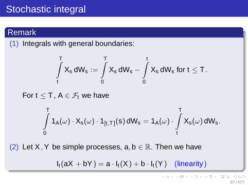
Stochastic integral
Remark(1) Integrals with general boundaries:
T∫
t
Xs dWs :=
T∫
0
Xs dWs −t∫
0
Xs dWs for t ≤ T .
For t ≤ T , A ∈ Ft we have
T∫
0
1A(ω) · Xs(ω) · 1[t,T ](s) dWs = 1A(ω) ·T∫
t
Xs(ω) dWs.
(2) Let X , Y be simple processes, a, b ∈ R. Then we have
It(aX + bY ) = a · It(X ) + b · It(Y ) (linearity)
87 / 477

Measurability
DefinitionA stochastic process (Xt , Gt)t∈[0,∞) is called measurable if themapping
[0,∞) × Ω → Rn
(s, ω) 7→ Xs(ω)
is B([0,∞)) ⊗F-B(Rn)-measurable.
RemarkMeasurability of the process X implies that X (., ω) isB([0,∞))-B(Rn)-measurable for a fixed ω ∈ Ω. Thus, for all t ∈ [0,∞),
i = 1, . . . , n, the integralt∫
0X 2
i (s) ds is defined.
88 / 477
Measurability
DefinitionA stochastic process (Xt , Gt)t∈[0,∞) is called progressivelymeasurable if for all t ≥ 0 the mapping
[0, t] × Ω → Rn
(s, ω) 7→ Xs(ω)
is B([0, t]) ⊗ Gt -B(Rn)-measurable.
89 / 477

Measurability
Remark(1) If the real-valued process (Xt , Gt)t∈[0,∞) is progressively
measurable and bounded, then for all t ∈ [0,∞) the integralt∫
0Xs ds is Gt -measurable.
(2) Every progressively measurable process is measurable.
(3) Each measurable process possesses a progressively measurablemodification.
90 / 477

Measurability
TheoremIf all paths of the stochastic process (Xt , Gt)t∈[0,∞) areright-continuous (or left-continuous), then the process is progressivelymeasurable.
TheoremLet τ be a stopping time with respect to the filtration Gtt∈[0,∞). If thestochastic process (Xt , Gt)t∈[0,∞) is progressively measurable, thenso is the stopped process (Xt∧τ , Gt)t∈[0,∞). In particular, Xt∧τ is Gt
and Gt∧τ -measurable.
91 / 477

Extension of the stochastic integral toL2[0, T ]-processes
Definition
L2[0, T ] := L2([0, T ],Ω,F , Ftt∈[0,T ], P
)
:=
(Xt ,Ft)t∈[0,T ] real-valued stochastic process
∣∣∣∣
Xtt progressively measurable, E( T∫
0
X 2t dt
)<∞
Norm on L2[0, T ]: ‖X‖2T := E
( T∫0
X 2t dt
).
92 / 477

Extension of the stochastic integral toL2[0, T ]-processes
‖ · ‖2T L2-norm on the probability space(
[0, T ]× Ω, B([0, T ]) ⊗F , λ ⊗ P).
‖ · ‖2T semi-norm (‖X − Y‖2
T = 0 6⇒ X = Y ).
X equivalent to Y :⇔ X = Y a.s. λ ⊗ P.
93 / 477

Extension of the stochastic integral toL2[0, T ]-processes
Ito isometryLet X be a simple process. The mapping X 7→ I.(X ) induces by
‖I.(X )‖2LT
:= E( T∫
0
Xs dWs
)2
= E( T∫
0
X 2s ds
)= ‖X‖2
T
a norm on the space of stochastic integrals.
⇒ I.(X ) linear, norm-preserving (= isometry)
⇒ I.(X ) Ito isometry
94 / 477

Extension of the stochastic integral toL2[0, T ]-processes
Use processes X ∈ L2[0, T ] approximated by a sequence X (n) ofsimple processes.
I.(X (n)) is a Cauchy-sequence with respect to ‖ · ‖LT.
To show: I.(X (n)) is convergent, limit independent of X (n).
Denote limit by
I(X ) =
∫Xs dWs.
95 / 477

Extension of the stochastic integral toL2[0, T ]-processes
X ∈ L2[0, T ]J(.) //_______ J(X ) ∈ MC
2
X (n)
‖·‖T
OO
I(.)// I(X (n))
‖·‖LT
OO
simple process stochastic integralfor simple processes
96 / 477
Extension of the stochastic integral toL2[0, T ]-processes
Theorem
An arbitrary X ∈ L2[0, T ] can be approximated by a sequence ofsimple processes X (n).
More precisely: There exists a sequence X (n) of simple processes with
limn→∞
E
T∫
0
(Xs − X (n)
s
)2ds = 0.
97 / 477
Extension of the stochastic integral toL2[0, T ]-processes
LemmaLet (Xt , Gt)t∈[0,∞) be a martingale where the filtration Gtt∈[0,∞)
satisfies the usual conditions. Then the process Xt possesses aright-continuous modification (Yt , Gt)t∈[0,∞) such that(Yt , Gt)t∈[0,∞) is a martingale.
98 / 477
Extension of the stochastic integral toL2[0, T ]-processes
Construction of the Ito integral for processes in L2[0, T ]
There exists a unique linear mapping J from L2[0, T ] into the space ofcontinuous martingales on [0, T ] with respect to Ftt∈[0,T ] satisfying
(1) X = Xtt∈[0,T ] simple process⇒ P
(Jt(X ) = It(X ) for all t ∈ [0, T ]
)= 1
(2) E(
Jt(X )2)
= E( t∫
0X 2
s ds)
Ito isometry
Uniqueness: If J, J ′ satisfy (1) and (2), then for all X ∈ L2[0, T ] theprocesses J ′(X ) and J(X ) are indistinguishable.
99 / 477

Extension of the stochastic integral toL2[0, T ]-processes
Definition
For X ∈ L2[0, T ] and J as before we define by
t∫
0
Xs dWs := Jt(X )
the stochastic integral (or Ito integral) of X with respect to W .
100 / 477

Extension of the stochastic integral toL2[0, T ]-processes
Theorem: Special case of Doob’s inequality
Let X ∈ L2[0, T ]. Then we have
E(
sup0≤t≤T
∣∣∣∣
t∫
0
Xs dWs
∣∣∣∣)2
≤ 4 · E( T∫
0
X 2s ds
).
101 / 477
Extension of the stochastic integral toL2[0, T ]-processes
Multi-dimensional generalization of the stochastic integral
(W (t), Ft)t : m-dimensional Brownian motionwith W (t) = (W1(t), . . . , Wm(t))
(X (t), Ft)t : Rn,m-valued progressively measurable process with
Xij ∈ L2[0, T ].
Ito integral of X with respect to W :
t∫
0
X (s) dW (s) :=
m∑
j=1
t∫
0
X1j(s) dWj(s)
...m∑
j=1
t∫
0
Xnj(s) dWj(s)
, t ∈ [0, T ]
102 / 477

Further extension of the stochastic integral
Definition
H2[0, T ] := H2([0, T ], Ω, F , Ftt∈[0,T ], P
)
:=
(Xt ,Ft)t∈[0,T ] real-valued stochastic process
∣∣∣∣
Xtt progressively measurable,
T∫
0
X 2t dt < ∞ P-a.s.
103 / 477

Further extension of the stochastic integral
Processes X ∈ H2[0, T ]
do not necessarily have a finite T -norm→ no approximation by simple processes as for
processes in L2[0, T ]
can be localized with suitable sequences of stopping times
Stopping times (with respect to Ftt ):
τn(ω) := T ∧ inf
0 ≤ t ≤ T
∣∣∣∣
t∫
0
X 2s (ω) ds ≥ n
, n ∈ N
Sequence of stopped processes:
X (n)t (ω) := Xt(ω) · 1τn(ω)≥t
⇒ X (n) ∈ L2[0, T ] ⇒ Stochastic integral already defined.
104 / 477

Further extension of the stochastic integral
Stochastic integral:
It(X ) := It(X (n)) for 0 ≤ t ≤ τn
Consistence property:
It(X ) = It(X (m)) for 0 ≤ t ≤ τn(≤ τm), m ≥ n
⇒ It(X ) well-defined for X ∈ H2[0, T ]
105 / 477

Further extension of the stochastic integral
Stopping times:τn
n→∞−−−→ +∞ P-a.s.
⇒ It(X ) local martingale with localizing sequence τn.
⇒ Stochastic integral is linear and possesses continuous paths.
106 / 477

Outline
2 The Continuous-Time Market ModelModeling the Security PricesExcursion 1: Brownian Motion and MartingalesContinuation: Modeling the Security pricesExcursion 2: The Ito IntegralExcursion 3: The Ito FormulaTrading Strategy and Wealth ProcessProperties of the Continuous-Time Market ModelExcursion 4: The Martingale Representation Theorem
107 / 477

The Ito formula
General assumptions for this sectionLet (Ω,F , P) be a complete probability space equipped with a filtrationFtt satisfying the usual conditions. Further, assume that on thisspace a Brownian motion (Wt ,Ft)t∈[0,∞) with respect to this filtrationis defined.
108 / 477
The Ito formula
DefinitionLet (Wt ,Ft)t∈[0,∞) be an m-dimensional Brownian motion.
(1) (X (t),Ft )t∈[0,∞) is a real-valued Ito process if for all t ≥ 0 itadmits the representation
X (t) = X (0) +
t∫
0
K (s) ds +
t∫
0
H(s) dW (s)
= X (0) +
t∫
0
K (s) ds +
m∑
j=1
t∫
0
Hj(s) dWj(s) P-a.s.
109 / 477
The Ito formula
X (0) F0-measurable,K (t)t∈[0,∞), H(t)t∈[0,∞) progressively measurable with
t∫
0
|K (s)|ds < ∞,
t∫
0
H2i (s) ds < ∞ P-a.s.
for all t ≥ 0, i = 1, . . . , m.
(2) n-dimensional Ito process X = (X (1), . . . , X (n))= vector with components being real-valued Ito processes.
110 / 477

The Ito formula
Remark
Hj ∈ H2[0, T ] for all T > 0.
The representation of an Ito process is unique up toindistinguishability of the representing integrands Kt , Ht .
Symbolic differential notation:
dXt = Kt dt + Ht dWt
111 / 477

The Ito formula
DefinitionLet X and Y be two real-valued Ito processes with
X (t) = X (0) +
t∫
0
K (s) ds +
t∫
0
H(s) dW (s),
Y (t) = Y (0) +
t∫
0
L(s) ds +
t∫
0
M(s) dW (s).
Quadratic covariation of X and Y :
〈X , Y 〉t :=
m∑
i=1
t∫
0
Hi(s) · Mi(s) ds.
112 / 477

The Ito formula
DefinitionQuadratic variation of X
〈X 〉t := 〈X , X 〉t .
NotationLet X be a real-valued Ito process, and Y a real-valued, progressivelymeasurable process. We set
t∫
0
Y (s) dX (s) :=
t∫
0
Y (s) · K (s) ds +
t∫
0
Y (s) · H(s) dW (s)
if all integrals on the right-hand side are defined.
113 / 477

The Ito formula
Theorem: One-dimensional Ito formulaLet Wt be a one-dimensional Brownian motion, and Xt a real-valued Itoprocess with
Xt = X0 +
t∫
0
Ks ds +
t∫
0
Hs dWs.
Let f ∈ C2(R). Then, for all t ≥ 0 we have
f (Xt) = f (X0) +
t∫
0
f ′(Xs) dXs +12
t∫
0
f ′′(Xs) d〈X 〉s
= f (X0) +
t∫
0
(f ′(Xs) · Ks +
12· f ′′(Xs) · H2
s
)ds +
t∫
0
f ′(Xs)Hs dWs
114 / 477

The Ito formula
RemarkThe Ito formula differs from the fundamental theorem of calculusby the additional term
12
t∫
0
f ′′(Xs) d〈X 〉s.
The quadratic variation 〈X 〉t is an Ito process.
Differential notation:
df (Xt) = f ′(Xt) dXt +12· f ′′(Xt) d〈X 〉t .
115 / 477

The Ito formula
LemmaLet X be a martingale with |Xs| ≤ C for all s ∈ [0, t] P-a.s.Let π = t0, t1, . . . , tm, t0 = 0, tm = t , be a partition of [0, t] with
‖π‖ := max1≤k≤m
|tk − tk−1|.
Then we have
(1) E( m∑
k=1
(Xtk − Xtk−1
)2)2
≤ 48 · C4
(2) X continuous ⇒ E( m∑
k=1
(Xtk − Xtk−1
)4)
‖π‖→0−−−−→ 0.
116 / 477
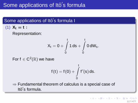
Some applications of Ito′s formula
Some applications of Ito′s formula I(1) Xt = t :
Representation:
Xt = 0 +
t∫
0
1 ds +
t∫
0
0 dWs.
For f ∈ C2(R) we have
f (t) = f (0) +
t∫
0
f ′(s) ds.
⇒ Fundamental theorem of calculus is a special case ofIto′s formula.
117 / 477

Some applications of Ito′s formula II
Some applications of Ito′s formula
(2) Xt = h(t) :
For h ∈ C1(R) Ito′s formula implies the chain rule
Xt = h(0) +
t∫
0
h′(s) ds +
t∫
0
0 dWs
⇒ (f h)(t) = (f h)(0) +
t∫
0
f ′(h(s)) · h′(s) ds.
118 / 477
Some applications of Ito′s formula III
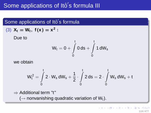
Some applications of Ito′s formula
(3) Xt = Wt , f (x) = x2 :
Due to
Wt = 0 +
t∫
0
0 ds +
t∫
0
1 dWs
we obtain
W 2t =
t∫
0
2 · Ws dWs +12·
t∫
0
2 ds = 2 ·t∫
0
Ws dWs + t
⇒ Additional term "t"(→ nonvanishing quadratic variation of Wt ).
119 / 477

The Ito formula
Theorem: Multi-dimensional Ito formula
X (t) =(X1(t), . . . , Xn(t)
)n-dimensional Ito process with
Xi(t) = Xi(0) +
t∫
0
Ki(s) ds +m∑
j=1
t∫
0
Hij(s) dWj(s), i = 1, . . . , n
where W (t) =(W1(t), . . . , Wm(t)
)is an m-dimensional Brownian motion.
Let f : [0,∞) × Rn → R be a C1,2-function. Then, we have
f (t , X1(t), . . . , Xn(t)) = f (0, X1(0), . . . , Xn(0))
+
t∫
0
ft(s, X1(s), . . . , Xn(s)) ds +
n∑
i=1
t∫
0
fxi (s, X1(s), . . . , Xn(s)) dXi(s)
+12·
n∑
i ,j=1
t∫
0
fxi xj (s, X1(s), . . . , Xn(s)) d〈Xi , Xj〉s.
120 / 477

Product rule or partial integration
Corollary: Product rule or partial integration
Let Xt , Yt be one-dimensional Ito processes with
Xt = X0 +
t∫
0
Ks ds +
t∫
0
Hs dWs,
Yt = Y0 +
t∫
0
µs ds +
t∫
0
σs dWs.
Then we have
Xt · Yt = X0 · Y0 +
t∫
0
Xs dYs +
t∫
0
Ys dXs +
t∫
0
d〈X , Y 〉s
= X0 · Y0 +
t∫
0
(Xsµs + YsKs + Hsσs
)ds +
t∫
0
(Xsσs + YsHs
)dWs.
121 / 477

The stock price equation
Simple continuous-time market model (1 bond, one stock).Stock price influenced by a one-dimensional Brownian motion
Price of the stock at time t :
P(t) = p · exp((
b − 12σ2)
t + σWt
)
Choose
Xt = 0 +
t∫
0
(b − 1
2σ2)
ds +
t∫
0
σ dWs, f (x) = p · ex
Ito formula implies
f (Xt) = p +
t∫
0
[f (Xs)(b − 1
2σ2) + 12 f (Xs) · σ2]ds +
t∫
0
f (Xs) · σ dWs
122 / 477
The stock price equation
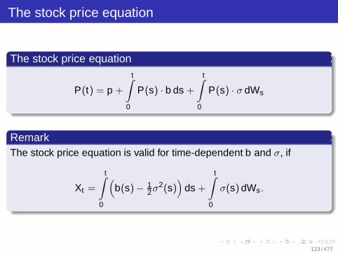
The stock price equation
P(t) = p +
t∫
0
P(s) · b ds +
t∫
0
P(s) · σ dWs
RemarkThe stock price equation is valid for time-dependent b and σ, if
Xt =
t∫
0
(b(s) − 1
2σ2(s))
ds +
t∫
0
σ(s) dWs.
123 / 477
The stock price equation
The stock price equation in differential form
dP(t) = P(t)(b dt + σ dWt
)
P(0) = p
124 / 477

The stock price equation
Theorem: Variation of constantsLet (W (t), Ft)t∈[0,∞) be an m-dimensional Brownian motion.Let x ∈ R and A, a, Sj , σj be progressively measurable, real-valuedprocesses with
t∫
0
(|A(s)| + |a(s)|
)ds < ∞ for all t ≥ 0 P-a.s.
t∫
0
(S2
j (s) + σ2j (s)
)ds < ∞ for all t ≥ 0 P-a.s. .
125 / 477
The stock price equation
Theorem: Variation of constantsThen the stochastic differential equation
dX (t) =(A(t) · X (t) + a(t)
)dt +
m∑
j=1
(Sj(t)X (t) + σj(t)
)dWj(t)
X (0) = x
possesses a unique solution with respect to λ ⊗ P :
X (t) = Z (t) ·(
x +
t∫
0
1Z (u)
(a(u) −
m∑
j=1
Sj(u)σj(u)
)du
+m∑
j=1
t∫
0
σj(u)
Z (u)dWj(u)
)
126 / 477
The stock price equation
Theorem: Variation of constantsHereby is
Z (t) = exp( t∫
0
(A(u) − 1
2 · ‖S(u)‖2) du +
t∫
0
S(u) dW (u)
)
the unique solution of the homogeneous equation
dZ (t) = Z (t)(A(t) dt + S(t)T dW (t)
)
Z (0) = 1.
127 / 477

The stock price equation
RemarkThe process (X (t), Ft)t∈[0,∞) solves the stochastic differentialequation in the sense that X (t) satisfies
X (t) = x +
t∫
0
(A(s) · X (s) + a(s)
)ds
+
m∑
j=1
t∫
0
(Sj(s) X (s) + σj(s)
)dWj(s)
for all t ≥ 0 P-almost surely.
128 / 477
Outline
2 The Continuous-Time Market ModelModeling the Security PricesExcursion 1: Brownian Motion and MartingalesContinuation: Modeling the Security pricesExcursion 2: The Ito IntegralExcursion 3: The Ito FormulaTrading Strategy and Wealth ProcessProperties of the Continuous-Time Market ModelExcursion 4: The Martingale Representation Theorem
129 / 477

General assumptions
General assumptions for this section(Ω,F , P) be a complete probability space,(W (t),Ft )t∈[0,∞) m-dimensional Brownian motion.
Dynamics of bond and stock prices:
P0(t) = p0 · exp( t∫
0
r(s) ds)
bond
Pi(t) = pi · exp( t∫
0
(bi(s) − 1
2
m∑
j=1
σ2ij (s)
)ds
+m∑
j=1
t∫
0
σij(s) dWj(s)
)stock
for t ∈ [0, T ], T > 0, i = 1, . . . , d .
130 / 477

General assumptions (continued)
General assumptions for this section (continued)
r(t), b(t) = (b1(t), . . . , bd (t))T , σ(t) = (σij(t))ij
progressively measurable processes with respect to Ftt ,component-wise uniformly bounded in (t , ω).
σ(t)σ(t)T uniformly positive definite,i.e., it exists K > 0 with
xT σ(t)σ(t)T x ≥ KxT x
for all x ∈ Rd and all t ∈ [0, T ] P-a.s.
Deterministic rate of return r(t) is not requiredr(t) can be a stochastic process⇒ bond is no longer riskless.
131 / 477
Bond and stock prices
Bond and stock prices are unique solutions of the stochasticdifferential equations
dP0(t) = P0(t) · r(t) dt bond
P0(t) = p0
dPi(t) = Pi(t)(
bi(t) dt +
m∑
j=1
σij(t) dWj(t))
, i = 1, . . . , d
Pi(0) = pi stock
⇒ Representations of prices as Ito processes
132 / 477

Possible actions of investors
(1) Investor can rebalance his holdings→ sell some securities→ invest in securities⇒ Portfolio process / trading strategy.
(2) Investor is allowed to consume parts of his wealth⇒ Consumption process.
133 / 477
Requirements on a market model
(1) Investor should not be able to foresee events→ no knowledge of future prices.
(2) Actions of a single investor have no impact on the stock prices(small investor hypothesis).
(3) Each investor has a fixed initial capital at time t = 0.
(4) Money which is not invested into stocks has to be invested inbonds.
(5) Investors act in a self-financing way(no secret source or sink for money).
134 / 477
Requirements on a market model
(6) Securities are perfectly divisible.
(7) Negative positions in securities are possiblebond → creditstock → we sold some stock short.
(8) No transaction costs.
135 / 477
Negative bond positions and credit interest rates
Negative bond positions and credit interest rates
Assume: Interest rate r(t) is constant
Negative bond position = it is possible to borrow money for thesame rate as we would get for investing in bonds.
Interest depends on the market situation ((t , ω) ∈ [0, T ] × Ω), butnot on positive or negative bond position.
136 / 477

Mathematical realizations of some requirements
Market with 1 bond and d stocks
Time t = 0: – Initial capital of investor: x > 0
– Buy a selection of securities
ϕ(0) =(ϕ0(0), ϕ1(0), . . . , ϕd(0)
)T
Time t > 0: – Trading strategy: ϕ(t)
(1) ⇒ trading strategy is progressively measurablewith respect to Ftt
Decisions on buying and selling are made on basis of informationavailable at time t (→ modelled by Ftt )
(5) ⇒ only self-financing trading strategies should be used.
137 / 477

Discrete-time example: self-financing strategy
Market with 1 riskless bond and 1 stock
Two-period model for time points t = 0, 1, 2.
Number of shares of bond and stock at time t :
(ϕ0(t), ϕ1(t))T ∈ R2
Consumption of investor at time t : C(t)
Wealth at time t : X (t)
Bond/stock prices at time t : P0(t), P1(t)
Initial conditions: C(0) = 0, X (0) = x
138 / 477
Discrete-time example: self-financing strategy
t = 0Investor uses initial capital to buy shares of bond and stock
X (0) = x = ϕ0(0) · P0(0) + ϕ1(0) · P1(0).
139 / 477

Discrete-time example: self-financing strategy
t = 1Security prices have changed, investor consumes parts of his wealth
Current wealth:
X (1) = ϕ0(0) · P0(1) + ϕ1(0) · P1(1) − C(1).
Total:
X (1) = x + ϕ0(0) ·(P0(1) − P0(0)
)+ ϕ1(0) ·
(P1(1) − P1(0)
)− C(1)
Wealth = initial wealth + gains/losses - consumption
Invest remaining capital at the market:
X (1) = ϕ0(1) · P0(1) + ϕ1(1) · P1(1).
140 / 477

Discrete-time example: self-financing strategy
t = 2Invest remaining capital at the market
Wealth:X (2) = ϕ0(2) · P0(2) + ϕ1(2) · P1(2).
Wealth = total wealth of shares held
Total:
X (2) = x +2∑
i=1
[ϕ0(i − 1) · (P0(i) − P0(i − 1))
+ϕ1(i − 1) · (P1(i) − P1(i − 1))]
−2∑
i=1
C(i).
141 / 477

Discrete-time example: self-financing strategy
Self-financing trading strategy:
wealth before rebalancing - consumption = wealth after rebalancing
Condition:
ϕ0(i) · P0(i) + ϕ1(i) · P1(i)
= ϕ0(i − 1) · P0(i) + ϕ1(i − 1) · P1(i) − C(i)
⇒ Useless in continuous-time setting
(securities can be traded at each time instant /"before" and "after" cannot be distinguished)
142 / 477

Discrete-time example: self-financing strategy
Continuous-time setting
Wealth process corresponding to strategy ϕ(t):
X (t) = x +
t∫
0
ϕ0(s) dP0(s) +
t∫
0
ϕ1(s) dP1(s) −t∫
0
c(s) ds
⇒ Price processes are Ito processes.
143 / 477

Trading strategy and wealth processes
Definition(1) A trading strategy ϕ with
ϕ(t) :=(ϕ0(t), ϕ1(t), . . . , ϕd (t)
)T
is an Rd+1-valued progressively measurable process with respect
to Ftt∈[0,T ] satisfying
T∫
0
|ϕ0(t)|dt < ∞ P-a.s.
d∑
j=1
T∫
0
(ϕi(t) · Pi(t)
)2 dt < ∞ P-a.s. for i = 1, . . . , d .
144 / 477
Trading strategy and wealth processes
DefinitionThe value
x :=
d∑
i=0
ϕi(0) · pi
is called initial value of ϕ.
(2) Let ϕ be a trading strategy with initial value x > 0.The process
X (t) :=d∑
i=0
ϕi(t)Pi (t)
is called wealth process corresponding to ϕ withinitial wealth x .
145 / 477
Trading strategy and wealth processes
Definition(3) A non-negative progressively measurable process c(t) with
respect to Ftt∈[0,T ] with
T∫
0
c(t) dt < ∞ P-a.s.
is called consumption (rate) process.
146 / 477
Trading strategy and wealth processes
DefinitionA pair (ϕ, c) consisting of a trading strategy ϕ and a consumption rateprocess c is called self-financing if the corresponding wealth processX (t) satisfies
X (t) = x +
d∑
i=0
t∫
0
ϕi(s) dPi(s) −t∫
0
c(s) ds P-a.s.
current wealth = initial wealth + gains/losses - consumption
147 / 477

Trading strategy and wealth processes
RemarkWe have
t∫
0
ϕ0(s) dP0(s) =
t∫
0
ϕ0(s) P0(s) r(s) ds
t∫
0
ϕi(s) dPi(s) =
t∫
0
ϕi(s) Pi(s) bi(s) ds
+
m∑
j=1
t∫
0
ϕi(s) Pi (s)σij(s) dWj(s), i = 1, . . . , d .
148 / 477

Self-financing portfolio process
DefinitionLet (ϕ, c) be a self-financing pair consisting of a trading strategy and aconsumption process with corresponding wealth process X (t) > 0P-a.s. for all t ∈ [0, T ]. Then the R
d -valued process
π(t) =(π1(t), . . . , πd (t)
)T with πi(t) =ϕi(t) · Pi(t)
X (t)
is called a self-financing portfolio process corresponding to thepair (ϕ, c).
149 / 477

Portfolio processes
Remark(1) The portfolio process denotes the fractions of total wealth invested
in the different stocks.
(2) The fraction of wealth invested in the bond is given by
(1 − π(t)T 1
)=
ϕ0(t) · P0(t)X (t)
, where 1 := (1, . . . , 1)T ∈ Rd .
(3) Given knowledge of wealth X (t) and prices Pi(t), it is possible foran investor to describe his activities via a self-financing pair (π, c).→ Portfolio process and trading strategy are
equivalent descriptions of the same action.
150 / 477
The wealth equation
The wealth equation
dX (t) = [r(t) X (t) − c(t)] dt
+ X (t)π(t)T ((b(t) − r(t) 1) dt + σ(t) dW (t))
X (0) = x
151 / 477

Alternative definition of a portfolio process
Definition
The progressively measurable Rd -valued process π(t) is called a
self-financing portfolio process corresponding to the consumptionprocess c(t) if the corresponding wealth equation possesses a uniquesolution X (t) = Xπ,c(t) with
T∫
0
(X (t) · πi(t)
)2 dt < ∞ P-a.s. for i = 1, . . . , d .
152 / 477

Admissibility
DefinitionA self-financing pair (ϕ, c) or (π, c) consisting of a trading strategy ϕ ora portfolio process π and a consumption process c will be calledadmissible for the initial wealth x > 0, if the corresponding wealthprocess satisfies
X (t) ≥ 0 P-a.s. for all t ∈ [0, T ].
The set of admissible pairs will be denoted by A(x).
153 / 477

An example
Portfolio process:π(t) ≡ π ∈ R
d constant
Consumption rate:c(t) = γ · X (t), γ > 0
Wealth process corresponding to (π, c) :
X (t)
Investor rebalances his holdings in such a way that the fractions ofwealth invested in the different stocks and in the bond remainconstant over time.
Consumption rate is proportional to the current wealth of theinvestor.
154 / 477

An example
Wealth equation:
dX (t) = [r(t) − γ] X (t) dt
+ X (t)πT ((b(t) − r(t) 1) dt + σ(t) dW (t))
X (0) = 0
Wealth process:
X (t) = x · exp( t∫
0
[r(s) − γ + πT (b(s) − r(s) · 1
)− 1
2‖πT σ(s)‖2
]ds
+
t∫
0
πT σ(s) dW (s)
)
155 / 477

Outline
2 The Continuous-Time Market ModelModeling the Security PricesExcursion 1: Brownian Motion and MartingalesContinuation: Modeling the Security pricesExcursion 2: The Ito IntegralExcursion 3: The Ito FormulaTrading Strategy and Wealth ProcessProperties of the Continuous-Time Market ModelExcursion 4: The Martingale Representation Theorem
156 / 477

Properties of the continuous-time market model
Assumptions:
Dimension of the underlying Brownian motion= number of stocks
Past and present prices are the only sources of information for theinvestors⇒ Choose Brownian filtration Ftt∈[0,T ]
Aim: Final wealths X (T ) when starting with initial capital of x .
157 / 477

General assumption / notation
General assumption for this section
d = m
Notation
γ(t) := exp(−
t∫
0
r(s) ds)
θ(t) := σ−1(t)(b(t) − r(t) 1
)
Z (t) := exp(−
t∫
0
θ(s)T dW (s) − 12
t∫
0
‖θ(s)‖2 ds)
H(t) := γ(t) · Z (t)
158 / 477
Properties of the continuous-time market model
b, r uniformly boundedσσT uniformly positive definite⇒ ‖θ(t)‖2 uniformly bounded
Interpretation of θ(t): Relative risk premium for stock investment.
Process H(t) is important for option pricing .
H(t) is positive, continuous, and progressively measurable withrespect to Ftt∈[0,T ].
H(t) is the unique solution of the SDE
dH(t) = −H(t)(r(t) dt + θ(t)T dW (t)
)
H(0) = 1.
159 / 477

Completeness of the market
Theorem: Completeness of the market(1) Let the self-financing pair (π, c) consisting of a portfolio process π
and a consumption process c be admissible for an initial wealth ofx ≥ 0, i.e.,
(π, c) ∈ A(x).
Then the corresponding wealth process X (t) satisfies
E(
H(t) X (t) +
t∫
0
H(s)c(s) ds)
≤ x for all t ∈ [0, T ].
160 / 477
Completeness of the market
Theorem: Completeness of the market(2) Let B ≥ 0 be an FT -measurable random variable and c(t) a
consumption process satisfying
x := E(
H(T ) B +
T∫
0
H(s)c(s) ds)
< ∞.
Then there exists a portfolio process π(t) with (π, c) ∈ A(x) andthe corresponding wealth process X (t) satisfies
X (T ) = B P-a.s.
161 / 477
Completeness of the market
H(t) can be regarded as the appropriate discounting process thatdetermines the initial wealth at time t = 0
E( T∫
0
H(s) · c(s) ds)
+ E(H(T ) · B)
which is necessary to attain future aims.
(1) puts bounds on the desires of an investor given his initialcapital x ≥ 0.
(2) proves that future aims which are feasible in the sense of part(1) can be realized.
(2) says that each desired final wealth in t = T can be attainedexactly via trading according to an appropriate self-financing pair(π, c) if one possesses sufficient initial capital(completeness/complete model) .
162 / 477
Completeness of the market
Remark1/H(t) is the wealth process corresponding to the pair
(π(t), c(t)
)=(σ−1(t)T θ(t), 0
)
with initial wealth x := 1/H(0) = 1
and final wealth B:= 1/H(T ).
163 / 477

Outline
2 The Continuous-Time Market ModelModeling the Security PricesExcursion 1: Brownian Motion and MartingalesContinuation: Modeling the Security pricesExcursion 2: The Ito IntegralExcursion 3: The Ito FormulaTrading Strategy and Wealth ProcessProperties of the Continuous-Time Market ModelExcursion 4: The Martingale Representation Theorem
164 / 477

Excursion 4: The martingale representation theorem
General assumptions(Ω,F , P) complete probability space.(Wt ,Ft)t∈[0,∞) m-dimensional Brownian motion.Ftt Brownian filtration.
DefinitionA real-valued martingale (Mt ,Ft)t∈[0,T ] with respect to the Brownianfiltration Ftt is called a Brownian martingale.
165 / 477
The martingale representation theorem
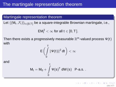
Martingale representation theorem
Let (Mt ,Ft)t∈[0,T ] be a square-integrable Brownian martingale, i.e.,
EM2t < ∞ for all t ∈ [0, T ].
Then there exists a progressively measurable Rm-valued process Ψ(t)
with
E( T∫
0
‖Ψ(t)‖2 dt)
< ∞
and
Mt = M0 +
t∫
0
Ψ(s)T dW (s) P-a.s. .
166 / 477
The martingale representation theorem
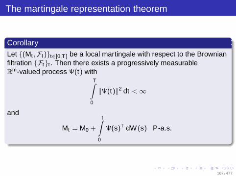
CorollaryLet (Mt ,Ft)t∈[0,T ] be a local martingale with respect to the Brownianfiltration Ftt . Then there exists a progressively measurableR
m-valued process Ψ(t) withT∫
0
‖Ψ(t)‖2 dt < ∞
and
Mt = M0 +
t∫
0
Ψ(s)T dW (s) P-a.s.
167 / 477

The martingale representation theorem
RemarkEach local martingale with respect to the Brownian filtration canbe represented as an Ito process.
Each Brownian martingale can be represented as an Ito process.
⇒ Quadratic variation and quadratic covariation are defined.
168 / 477

Outline
3 Option Pricing
169 / 477

Outline
3 Option PricingIntroductionExamplesThe Replication PrincipleArbitrage OpportunityContinuationPartial Differential Approach (PDA)Arbitrage & Option Pricing
170 / 477
Introduction
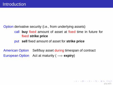
Option derivative security (i.e., from underlying assets)
call buy fixed amount of asset at fixed time in future forfixed strike price
put sell fixed amount of asset for strike price
American Option Sell/buy asset during timespan of contract
European Option Act at maturity ( =⇒ expiry )
171 / 477

Outline
3 Option PricingIntroductionExamplesThe Replication PrincipleArbitrage OpportunityContinuationPartial Differential Approach (PDA)Arbitrage & Option Pricing
172 / 477

European call
European callRight to buy security at time t = T for strike price K > 0fixed at time t = 0
P(T ) > K Gain (P(T ) − K )+
P(T ) ≤ K No gain (Holder will buy in market)
173 / 477

European put
European putRight to sell security at time t = T for price K > 0 fixed at time t = 0
P(T ) ≥ K No gain (Holder will sell in market)
P(T ) < K Gain (K − P(T ))+
174 / 477

The payoff diagram
The payoff diagramGraph of final gain (through the option) as function of the stock price attime T
175 / 477

Payoff diagram of a call
P1(T)
(P1(T)−K)+
K
K0
176 / 477

Payoff diagram of a put
P1(T)
(K−P1(T))+
K
K0
177 / 477

The sense of options
Hedge against price fluctuations of underlying asset
Bound risks of future cash flows
Risks of option speculationHigh losses not unusual
178 / 477

Outline
3 Option PricingIntroductionExamplesThe Replication PrincipleArbitrage OpportunityContinuationPartial Differential Approach (PDA)Arbitrage & Option Pricing
179 / 477

Option pricing
Option PricingBond Interest Rate (BIR) r constant
Fixed deterministic payment of B at time T has present value of
e−rT · B
Sum to be invested at t = 0 to obtain amount of B at maturity.
180 / 477

Option pricing
Option Pricing
BIR r(t) time dependent and random variableExpected value
E(
e−
T∫
0r(s) ds
· B)
181 / 477
Examples of option pricing
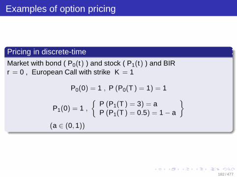
Pricing in discrete-time
Market with bond ( P0(t) ) and stock ( P1(t) ) and BIRr = 0 , European Call with strike K = 1
P0(0) = 1 , P (P0(T ) = 1) = 1
P1(0) = 1 ,
P (P1(T ) = 3) = aP (P1(T ) = 0.5) = 1 − a
(a ∈ (0, 1))
182 / 477
Examples of option pricing
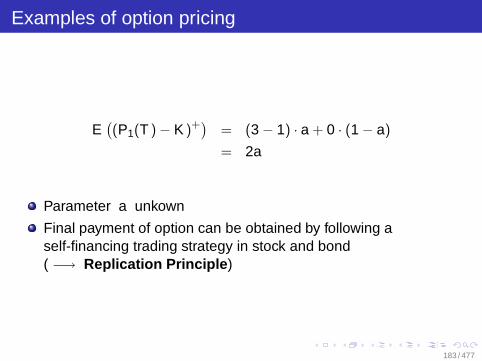
E((P1(T ) − K )+
)= (3 − 1) · a + 0 · (1 − a)
= 2a
Parameter a unkown
Final payment of option can be obtained by following aself-financing trading strategy in stock and bond( −→ Replication Principle )
183 / 477

Examples of option pricing
Determine (ϕ0(0), ϕ1(0)) such that
X (T ) = ϕ0(0) · P0(T ) + ϕ1(0) · P1(T )
= (P1(T ) − K )+
184 / 477

Examples of option pricing
Option Price
p = ϕ0(0) · P0(0) + ϕ1(0) · P1(0)
equals capital in t = 0 to buy replication strategy (ϕ0(0), ϕ1(0))
For all other choices riskless gains are possible without initialcapital −→ arbitrage opportunities
185 / 477
Examples of option pricing
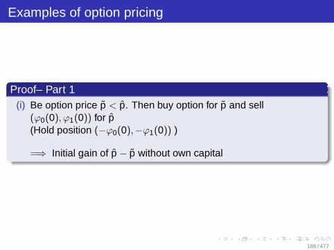
Proof– Part 1(i) Be option price p < p. Then buy option for p and sell
(ϕ0(0), ϕ1(0)) for p(Hold position (−ϕ0(0),−ϕ1(0)) )
=⇒ Initial gain of p − p without own capital
186 / 477
Examples of option pricing
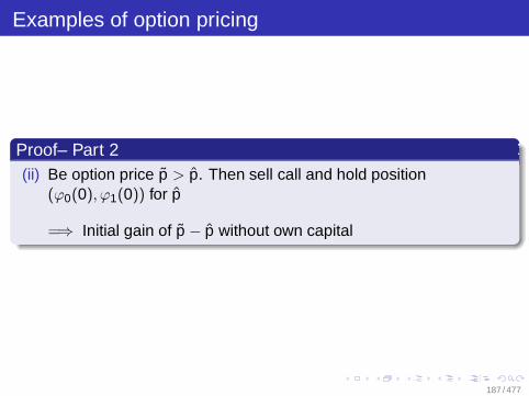
Proof– Part 2(ii) Be option price p > p. Then sell call and hold position
(ϕ0(0), ϕ1(0)) for p
=⇒ Initial gain of p − p without own capital
187 / 477

Examples of option pricing
Our example yields the system of equations
ϕ0(0) · 1 + ϕ1(0) · 3 = 2
ϕ0(0) · 1 + ϕ1(0) · 0.5 = 0
with unique solution
(ϕ0(0), ϕ1(0)) = (−0.4, 0.8)
=⇒ Option price p = −0.4 · 1 + 0.8 · 1 = 0.4
188 / 477

Examples of option pricing
Option price independent of unknown probability a
No arbitrage opportunities in market
Calculated call price p equals expected discounted terminalpayment of call ⇐⇒ a = 0.2−→ P1(t) is martingale
189 / 477

General assumptions
Assumptions for this sectionSelf-financing pair (π, c) ∈ A(x) admissible for initial capital x ≥ 0
190 / 477

Outline
3 Option PricingIntroductionExamplesThe Replication PrincipleArbitrage OpportunityContinuationPartial Differential Approach (PDA)Arbitrage & Option Pricing
191 / 477

Arbitrage opportunity
DefinitionBe
(ϕ, c) a self-financing and admissible pair
ϕ a trading strategy
c a consumption process
(ϕ, c) is called arbitrage opportunity ⇐⇒ corresponding wealthprocess satisfies
192 / 477

Arbitrage opportunity
Definition continued
X (0) = 0 , X (T ) ≥ 0 P-a.s.
P (X (T ) > 0) > 0 or P
T∫
0
c(t) dt > 0
> 0
193 / 477

Arbitrage opportunity
CorollaryIn the complete continuous-time market model there is no arbitrageopportunity.
194 / 477

Contingent claim
DefinitionA contingent claim (g, B) consists of an Ftt -progressivelymeasurable payout rate process g(t), t ∈ [0, T ], g(t) ≥ 0, and aFT -measurable terminal payment B ≥ 0 at T with
E
T∫
0
g(t) dt + B
µ < ∞
for some µ > 1.
195 / 477

Replication strategy
Definition(π, c) is called replication strategy for the contingent claim (g, B) if
g(t) = c(t) P-a.s. ∀ t ∈ [0, T ]
X (T ) = B P-a.s.
where X (t) is wealth process corresponding to (π, c).
196 / 477

Set of replication strategies of price x
Definition
D(x) := D (x ; (g, B))
:= (π, c) ∈ A(x)| (π, c) replication
strategy for (g, B)
197 / 477

Fair price
DefinitionThe fair price of the contingent claim (g, B) is defined as
p := inf p | D(p) 6= ∅ .
198 / 477
Fair price of contingent claim (g, B)
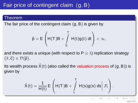
TheoremThe fair price of the contingent claim (g, B) is given by
p = E
H(T )B +
T∫
0
H(t)g(t) dt
< ∞,
and there exists a unique (with respect to P ⊗ λ) replication strategy(π, c
)∈ D
(p).
Its wealth process X (t) (also called the valuation process of (g, B)) isgiven by
X (t) =1
H(t)E
H(T )B +
T∫
t
H(s)g(s) ds
∣∣∣∣ Ft
.
199 / 477
The valuation process
RemarkThe above theorem gives us the fair price of the contingent claim(g, B) at time t as this price p(t) has to coincide with X (t). Otherwise,there would be arbitrage opportunities in the market consisting ofstock, bond, and contingent claim.
200 / 477

Black-Scholes formula
TheoremConsider a market model with just one stock and a bond with constantmarket coefficients, i.e.,
d = m = 1
andr(t) ≡ r , b(t) ≡ b , σ(t) ≡ σ > 0
for all t ∈ [0, T ], T > 0, r , b, σ ∈ R.
201 / 477

Black-Scholes formula
(i) The price XC(t) of a European call with strike price K > 0 andmaturity T is given by
XC(t) = P1(t)Φ(d1(t)) − Ke−r(T−t)Φ(d2(t))
d1(t) =ln(
P1(t)K
)+ (r + 0.5σ2)(T − t)
σ√
T − t
d2(t) =ln(
P1(t)K
)+ (r − 0.5σ2)(T − t)
σ√
T − t
= d1(t) − σ√
T − t
where Φ is the distribution function of the standard normaldistribution.
202 / 477
Black-Scholes formula
(ii) Price XP(t) of European put with strike K > 0
XP(t) = Ke−r(T−t)Φ(−d2(t)) − P1(t)Φ(−d1(t)).
203 / 477

The change of measure
W Q(t) := W (t) + θt =⇒
p = XC(0) = EQ
(e−rT (P1(T ) − K )+
)
where EQ(·) denotes expected value with respect to measure Q givenby Radon-Nikodym derivative
dQdP
= e−0.5θ2T−θW (T ).
204 / 477

General assumptions of this section
General Assumptions of this SectionBe (X (t),Ft )t≥0 an m-dimensional progressively measurableprocess, Ft the Brownian filtration with
t∫
0
X 2i (s) ds < ∞ P-a.s. for all t ≥ 0, i = 1, . . . , m.
Let further
Z (t , X ) := exp(−
m∑
i=1
t∫
0
Xi(s) dWi(s) − 12
t∫
0
‖X (s)‖2 ds)
.
205 / 477

Consequences
The argument in Z (t , X ) is an Ito process and we have
Z (t , X ) = 1 −m∑
i=1
t∫
0
Z (s, X )Xi(s) dWi(s).
Z (t , X ) is a continuous local martingale with Z (0, X ) = 1.
206 / 477

Girsanov’s theorem
Girsanov’s theoremBe process Z (t , X ) a martingale and define process(
W Q(t),Ft)
t≥0 by
W Qi (t) := Wi(t) +
t∫
0
Xi(s) ds (1 ≤ i ≤ m, t ≥ 0)
Then, for each fixed T ∈ [0,∞) the process(
W Q(t),Ft)
t∈[0,T ]is
an m-dimensional Brownian motion on (Ω,FT , QT ) with probabilitymeasure
QT (A) := E (1A · Z (T , X )) ∀ A ∈ FT
207 / 477

The Novikov condition
Z (t , X ) martingale −→ apply Girsanov’s theorem
Sufficient condition is the Novikov condition:
E(
e0.5
t∫
0‖X(s)‖2 ds
)< ∞
208 / 477

The Novikov condition
Proposition
If we haveT∫0
‖X (s)‖2 ds < K for some constant K > 0, then
Z (t , X ) is a martingale.
209 / 477

Outline
3 Option PricingIntroductionExamplesThe Replication PrincipleArbitrage OpportunityContinuationPartial Differential Approach (PDA)Arbitrage & Option Pricing
210 / 477

Girsanov’s theorem & Option Pricing
LemmaBe Q a probability measure which is equivalent to P restricted onFT . Then the density process Dtt∈[0,T ] defined by
Dt :=dQdP
∣∣∣∣Ft
, t ∈ [0, T ]
satisfies: (Dt ,Ft)t∈[0,T ] is a positive Brownian martingale withrespect to P satisfying
Dt = 1 +
∫ t
0Ψ(s)T dW (s)
for a progressively measurable d -dimensional process Ψ with
T∫
0
‖Ψ(s)‖2 ds < ∞ P-a.s.
211 / 477

Uniqueness of the equivalent martingale measure
TheoremIn the complete market model QT is the unique equivalent martingalemeasure on Ftt∈[0,T ] for the price processes Pi(t), 0 ≤ i ≤ d .
RemarkThe existence of an equivalent martingale measure implies theabsence of arbitrage opportunities in the market.
The absence of arbitrage implies the existence of an equivalentmartingale measure.
212 / 477
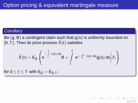
Option pricing & equivalent martingale measure
CorollaryBe (g, B) a contingent claim such that g(s) is uniformly bounded on[0, T ]. Then its price process X (t) satisfies
X (t) = EQ
e
−T∫t
r(s) dsB +
T∫
t
e−∫ s
t r(u) dug(s) ds
∣∣∣∣Ft
for 0 ≤ t ≤ T with EQ = EQ,T .
213 / 477

Independence of the option price
In the case of g ≡ 0 we have
p = EQ
e
−T∫
0r(s) ds
B
Thus, p equals the natural price with respect to a new (uniquelydetermined) probability measure Q.
214 / 477
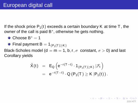
European digital call
If the shock price P1(t) exceeds a certain boundary K at time T , theowner of the call is paid B∗, otherwise he gets nothing.
Choose B∗ = 1
Final payment B = 1P1(T )≥KBlack-Scholes model (d = m = 1, b, r , σ constant, σ > 0) and lastCorollary yields
X(t) = EQ
(e−r(T−t) · 1P1(T )≥K |Ft
)
= e−r(T−t) · Q (P1(T ) ≥ K |P1(t) ) .
215 / 477

European digital call
For fixed t we have P1(T ) ≥ K ⇐⇒
W Q(T ) − W Q(t) ≥ln(
KP1(t)
)−(
r − σ2
2
)(T − t)
σ︸ ︷︷ ︸:=K
As W Q(T ) − W Q(t) is normally distributed with expectation 0 andvariance T − t , we obtain
216 / 477

European digital call
X (t) = e−r(T−t)∫ ∞
K
1√2π(T − t)
e− x2
2(T−t) dx
= e−r(T−t) Φ
ln(
P1(t)K
)+(
r − σ2
2
)(T − t)
σ√
T − t
217 / 477

Outline
3 Option PricingIntroductionExamplesThe Replication PrincipleArbitrage OpportunityContinuationPartial Differential Approach (PDA)Arbitrage & Option Pricing
218 / 477
Option pricing by PDA
General Assumptions nowConsider a Black-Scholes model, i.e.,
d = m = 1
andb, r , σ constant with σ > 0.
219 / 477
Option pricing by PDA
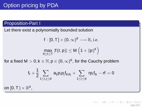
Proposition-Part ILet there exist a polynomially bounded solution
f : [0, T ]× (0,∞)d −→ R, i.e.
max0≤t≤T
|f (t , p)| ≤ M(
1 + ‖p‖k)
for a fixed M > 0, k ∈ N, p ∈ (0,∞)d , for the Cauchy problem
ft +12
∑
1≤i ,j≤d
aijpipj fpi pj +∑
1≤i≤d
rpi fpi − rf = 0
on [0, T ) × Rd ,
220 / 477
Option pricing by PDA
Proposition–Part II
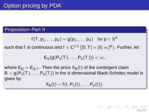
f (T , p1, . . . , pd ) = g(p1, . . . , pd ) for p ∈ Rd
such that f is continuous and f ∈ C1,2([0, T ] × (0,∞)d
). Further, let
EQ(g(P1(T ), . . . , Pd (T ))) < ∞,
where EQ = EQ,T . Then the price XB(t) of the contingent claimB = g(P1(T ), . . . , Pd(T )) in the d -dimensional Black-Scholes model isgiven by
XB(t) = f (t , P1(t), . . . , Pd (t)).
221 / 477

Option pricing by PDA
Proposition–Part IIIFurther for 1 ≤ i ≤ d ,
Ψi(t) = fpi (t , P1(t), . . . , Pd (t))
Ψ0(t) =
f (t , P1(t), . . . , Pd (t)) − ∑1≤i≤d
Ψi(t)Pi(t)
P0(t)
is a replication strategy for B.
222 / 477

SDE
Definition–Part IIf on (Ω,F , P) there exists a d -dimensional continuous process(X (t),Ft )t≥0 with X (0) = x , x ∈ R
d fixed,
Xi(t) = xi +
t∫
0
bi(s, X (s)) ds +∑
0≤j≤m
t∫
0
σij(s, X (s)) dWj(s)
P-a.s. for all t ≥ 0, 1 ≤ i ≤ d , satisfying
t∫
0
|bi(s, X (s))| +
∑
1≤j≤m
σ2ij (s, X (s))
ds < ∞
P-a.s. for all t ≥ 0, 1 ≤ i ≤ d ,
223 / 477

SDE
Definition–Part IIthen X (t) is called a strong solution of the stochastic differentialequation (SDE)
dX (t) = b(t , X (t)) dt + σ(t , X (t)) dW (t)
X (0) = x
whereb : [0,∞) × R
d −→ Rd , σ : [0,∞) × R
d −→ Rd ,m
are given functions (m dimension of Brownian motion).
224 / 477
Existence and uniqueness of solutions of SDEs
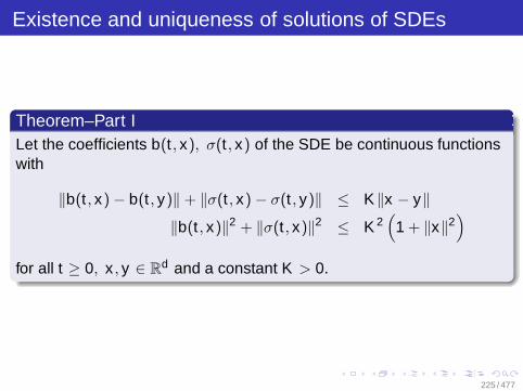
Theorem–Part ILet the coefficients b(t , x), σ(t , x) of the SDE be continuous functionswith
‖b(t , x) − b(t , y)‖ + ‖σ(t , x) − σ(t , y)‖ ≤ K‖x − y‖‖b(t , x)‖2 + ‖σ(t , x)‖2 ≤ K 2
(1 + ‖x‖2
)
for all t ≥ 0, x , y ∈ Rd and a constant K > 0.
225 / 477
Existence and uniqueness of solutions of SDEs
Theorem–Part IIThen there exists a continuous, strong solution (X (t),Ft )t≥0 of theSDE with
E(‖X (t)‖2
)≤ C
(1 + ‖x‖2
)eCT ∀ t ∈ [0, T ]
for some constant C = C(K , T ) and T > 0. Further, X (t) is unique upto indistinguishability.
226 / 477
Existence and uniqueness of solutions of SDEs
Proof planUniqueness
Existence – some estimates
Existence – convergence of the iteration
Solution property
227 / 477
Existence and uniqueness of solutions of SDEs
LemmaThe solution X of the SDE satisfies for m ≥ 1 and fixed T > 0
E(
max0≤s≤t
‖X (s)‖2m)
≤ C(
1 + ‖x‖2m)
eCt
for all t ∈ [0, T ] and suitable constant C = C(T , K , m, d).
Notation
Solution of the SDE with X (t) = x denote X t,s(s)
E(. . . X t,s(s) . . .) = E t,s(. . . X (s) . . .)
228 / 477

SDEs
DefinitionBe X (t) unique solution of the SDE under the introduced conditions.For f : R
d −→ Rd , f ∈ C2
(R
d), the operator At defined by
(At f )(x) :=12
∑
1≤i≤d
∑
1≤k≤d
aik (t , x)∂2f
∂xi∂xk(x)
+∑
1≤i≤d
bi(t , x)∂f∂xi
(x)
withaik (t , x) :=
∑
1≤j≤m
σij(t , x)σkj (t , x)
is called the characteristic operator corresponding to X (t).
229 / 477

The Cauchy problem
Description of the Cauchy problem IBe T > 0 fixed. Consider the following Cauchy problem correspondingto operator At :Find a function v(t , x) : [0, T ]× R
d −→ R with
−vt + kv = Atv + g on [0, T ] × Rd
v(T , x) = f (x) for x ∈ Rd
where
f : Rd −→ R , g : [0, T ] × R
d −→ R , k : [0, T ] × Rd −→ (0,∞).
230 / 477

The Cauchy problem
Description of the Cauchy problem IITo ensure the uniqueness of a solution we require that v obeys apolynomial growth condition:
max0≤t≤T
|v(t , x)| ≤ M(
1 + ‖x‖2µ)
with M > 0 , µ ≥ 1.
231 / 477
The Cauchy problem
Description of the Cauchy problem IIIUsually we assume that for suitable constants L, λ the functions f , g, kare continuous with
|f (x)| ≤ L(
1 + ‖x‖2λ)
, L > 0, λ ≥ 1 or f (x) ≥ 0
|g(t , x)| ≤ L(
1 + ‖x‖2λ)
, L > 0, λ ≥ 1 or g(t , x) ≥ 0.
232 / 477

The Feynman-Kac representation
Theorem–Part ILet the inequalities for f and g be satisfied. Let furtherv(t , x) : [0, T ] × R
d −→ R be continuous solution of the Cauchyproblem with v ∈ C1,2([0, T ) × R
d). Denote by At the characteristicoperator corresponding to the unique solution X (t) of the SDE withcontinuous coefficients b, σ with
bi(t , x), σ(t , x) : [0,∞) × Rd −→ R
for 1 ≤ i ≤ d , 1 ≤ j ≤ m.
233 / 477

The Feynman-Kac representation
Theorem–Part IIIf v(t , x) satisfies the polynomial growth condition we have therepresentation
v(t , x) = E t,x
f (X (T )) e
−T∫t
k(θ,X(θ)) dθ
+
+
T∫
t
g(s, X (s)) e−
s∫t
k(θ,X(θ)) dθ
ds
.
In particular, v(t , x) is unique solution.
234 / 477

Outline
3 Option PricingIntroductionExamplesThe Replication PrincipleArbitrage OpportunityContinuationPartial Differential Approach (PDA)Arbitrage & Option Pricing
235 / 477
General assumptions
General AssumptionsConsider market with d + 1 traded securities with positive pricesP0(t), . . . , Pd (t). Prices shall be Ito processes with respect to anm-dimensional Brownian motion (Wt ,Ft)t∈[0,∞) with m ≥ d whereFtt∈[0,∞) is the Brownian filtration.
236 / 477

General assumptions
Notations
As trading strategy ϕ(t) = (ϕ0(t), . . . , ϕd (t))T , t ≥ 0, define a(d + 1)-dimensional progressively measurable process such that thestochastic integrals
T∫
0
ϕi(s) dPi(s) ,
T∫
0
ϕi(s) dPi(s), 0 ≤ i ≤ d
exist for all T ≥ 0 where
Pi(t) :=Pi(t)P0(t)
denotes the discounted price process.
237 / 477
General assumptions
NotationsWealth process X (t) corresponding to the trading strategy ϕ(t) and theself-financing condition are defined by
X (t) =∑
0≤i≤d
ϕi(t)Pi(t)
= x +∑
0≤i≤d
t∫
0
ϕi(s) dPi(s)
P-a.s., for all t ≥ 0.
238 / 477
Equivalent martingale measures
DefinitionA probability measure Q defined on (Ω,FT ) equivalent to P (P and Qhave same zero sets) is called an equivalent martingale measure forP0(t), . . . , Pd (t) if the discounted prices
Pi(t) =Pi(t)P0(t)
(1 ≤ i ≤ m), t ∈ [0, T ]
are martingales with respect to Q.
239 / 477
Equivalent martingale measures
TheoremAll martingale measures Q for P0(t), . . . , Pd (t) equivalent to P can beobtained from P by a Girsanov transformation with an m-dimensionalprogressively measurable stochastic process (θ(t),Ft )t≥0 where forall t ≥ 0 we have
t∫
0
θ2i (s) ds < ∞ P-a.s. (1 ≤ i ≤ m)
and where Z (t , θ) is a martingale with respect to P.In particular, Q is given as
Q(A) := QT (A) := E(1A · Z (T , θ)) ∀ A ∈ FT .
240 / 477
Equivalent martingale measures =⇒ no arbitrage
TheoremIf there exists an equivalent martingale measure then the market givenby the price process P0(t), . . . , Pd(t) contains no arbitrage opportunity.
241 / 477
Completeness of the market
Definition(i) A contingent claim B is a non-negative FT -measureable random
variable with
EQ
(1
P0(T )B)
< ∞
for all equivalent martingale measures Q.
(ii) B is called attainable if there exists an admissible trading strategyϕ(t) with wealth process X (t) and
B = X (T ) P-a.s.
such that X (t) = X (t)/P0(t) is martingale with respect to someequivalent martingale measure Q.
242 / 477

Completeness of the market
TheoremThe security market under examination is complete (i.e. eachcontingent claim is attainable) if and only if there exists a uniqueequivalent martingale measure Q.
243 / 477
Option pricing in incomplete markets
DefinitionA market in which not every contingent claim is attainable is calledincomplete.
Possible reasons for incomplete markets can be
trading constraints to invest into particular stock.
additional random fluctuations in the market coefficients.
In an incomplete market, typically the σ-algebra FT is bigger than theone generated by final wealths produced by admissible tradingstrategies
X (T ) = x +∑
0≤i≤d
T∫
0
ϕi (s) dPi(s).
244 / 477

Prices of attainable contingent claims
TheoremThe unique price process X ∗(t) of an attainable contingent claim B isgiven by
X ∗(t) = EQ
(P0(t)P0(T )
B
∣∣∣∣Ft
)(t ∈ [0, T ]),
where Q is an equivalent martingale measure.
245 / 477

Option price and equivalent martingale measure
TheoremLet Q be an equivalent martingale measure to P. Let B be an arbitrarynot necessary attainable contingent claim. If we choose
X QB (t) := EQ
(P0(t)P0(T )
B
∣∣∣∣Ft
)
as price of the contingent claim then the extended security marketconsisting of d + 1 securities and the contingent claim contains noarbitrage opportunity.
246 / 477

Market numeraire and numeraire invariance
DefinitionLet (Y (t),Ft )t∈[0,T ] be a strictly positive Ito process and discountprocess. Then we call such a discount process a numeraire.
Questions:
Does change of numeraire (i.e., the choice of a numerairedifferent from P0(t)) affect the option price or its calculation?
Does there exist a numeraire such that the option price is given asexpected value of final payment B with respect to originalmeasure P when discounted by this numeraire?
247 / 477

Market numeraire and numeraire invariance
General AssumptionsConsider the complete market model with d = m and
1H(t)
= exp( t∫
0
(r(s) +
12‖θ(s)‖2
)ds +
t∫
0
θ(s)T dW (s)
).
By using the product rule and the SDE of the stock prices, we canverify that H(t) · Pi(t) are P-martingales for 0 ≤ i ≤ d .
1H(t) forms the wealth process corresponding to the admissible
pair (π, c) = (σ(t)−1(b(t) − r(t) 1), 0) ∈ A(1).
This numeraire can be replicated at market by trading in suitableway (market numeraire/numeraire portfolio).
248 / 477

Option price and equivalent martingale measure
Theorem
In complete market 1H(t) is the unique numeraire such that the
corresponding discounted price processes H(t) Pi(t), 0 ≤ i ≤ d , aremartingales with respect to P.
249 / 477

Numeraire invariance in the complete market
TheoremConsider the complete market model with constant market coefficientsr(t) ≡ r , b(t) ≡ b, σ(t) ≡ σ > 0. Then we have
(i) The process ZY (t) = H(t) Y π(t) is P-martingale for all constantportfolio processes π(t) ≡ π, where Y π(t) is wealth processcorresponding to π.
(ii) The corresponding probability measure QY with ZY (T ) = dQYdP is
unique equivalent martingale measure for price processesdiscounted by Y π(t).
(iii) Fair price p of a contingent claim B with E(Bµ) < ∞ for someµ > 1 is given as
p = E(H(T )B) = E(
1Yπ(T )
B)
if Y π(t) is numeraire of part (i)/(ii).
250 / 477

Outline
4 Pricing of Exotic Options and Numerical Algorithms
251 / 477
Outline
4 Pricing of Exotic Options and Numerical AlgorithmsIntroductionExamplesExamplesEquivalent Martingale MeasureExotic Options with Explicit Pricing FormulaeWeak Convergence of Stochastic ProcessesMonte-Carlo SimulationApproximation via Binomial TreesThe Pathwise Binomial Approach of Rogers and Stapleton
252 / 477

General assumptions
General assumptionsConsider a Black-Scholes model with d = m and constantcoefficients b, r , σ with σ > 0 (or σ regular if d > 1).
All options are assumed to be of European type.
253 / 477
Outline
4 Pricing of Exotic Options and Numerical AlgorithmsIntroductionExamplesExamplesEquivalent Martingale MeasureExotic Options with Explicit Pricing FormulaeWeak Convergence of Stochastic ProcessesMonte-Carlo SimulationApproximation via Binomial TreesThe Pathwise Binomial Approach of Rogers and Stapleton
254 / 477
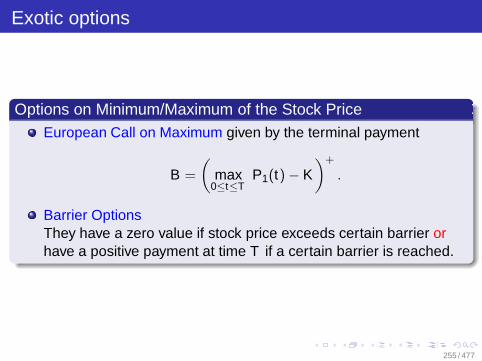
Exotic options
Options on Minimum/Maximum of the Stock PriceEuropean Call on Maximum given by the terminal payment
B =
(max
0≤t≤TP1(t) − K
)+
.
Barrier OptionsThey have a zero value if stock price exceeds certain barrier orhave a positive payment at time T if a certain barrier is reached.
255 / 477

Outline
4 Pricing of Exotic Options and Numerical AlgorithmsIntroductionExamplesExamplesEquivalent Martingale MeasureExotic Options with Explicit Pricing FormulaeWeak Convergence of Stochastic ProcessesMonte-Carlo SimulationApproximation via Binomial TreesThe Pathwise Binomial Approach of Rogers and Stapleton
256 / 477

Some examples for exotic options
Down-and-out Call
B = (P1(T ) − K1)+ 1
min0≤t≤T
P1(t)>K2
Down-and-in Call
B = (P1(T ) − K1)+ 1
min0≤t≤T
P1(t)≤K2
Double-barrier Call
B = (P1(T ) − K1)+ 1
min0≤t≤T
P1(t)>K2 , max0≤t≤T
P1(t)<K3
with K2 < K1 < K3.
257 / 477

Outline
4 Pricing of Exotic Options and Numerical AlgorithmsIntroductionExamplesExamplesEquivalent Martingale MeasureExotic Options with Explicit Pricing FormulaeWeak Convergence of Stochastic ProcessesMonte-Carlo SimulationApproximation via Binomial TreesThe Pathwise Binomial Approach of Rogers and Stapleton
258 / 477

Price of European option
The price of a European option is given by
p = EQ
(e−rT B
),
where Q is unique equivalent martingale measure andEQ its expectation.
AssumeStock prices are given as solutions of the SDE (1 ≤ i ≤ d)
dPi(t) = Pi(t)
r dt +
∑
1≤j≤d
σij dWj(t)
.
259 / 477

Outline
4 Pricing of Exotic Options and Numerical AlgorithmsIntroductionExamplesExamplesEquivalent Martingale MeasureExotic Options with Explicit Pricing FormulaeWeak Convergence of Stochastic ProcessesMonte-Carlo SimulationApproximation via Binomial TreesThe Pathwise Binomial Approach of Rogers and Stapleton
260 / 477

Path independent options on one stock
Binary Option–Part ITerminal payment in T of binary option with bound K given by
BCalld = 1P1(T )>K , BPut
d = 1P1(T )<K
if the final price P1(T ) exceeds K (in the case of a call) or issmaller than K (in the case of a put).
261 / 477
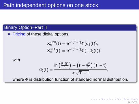
Path independent options on one stock
Binary Option–Part IIPricing of these digital options
X Calld (t) = e−t(T−t)Φ
(d2(t)
),
X Putd (t) = e−t(T−t)Φ
(−d2(t)
)
with
d2(t) =ln(
P1(t)K
)+(
r − σ2
2
)(T − t)
σ√
T − t,
where Φ is distribution function of standard normal distribution.
262 / 477

Path independent options on one stock
Paylater Options–Part IFinal payoffs
BCallPL =
(P1(T ) −
(K + DCall
))· 1P1(T )≥ K
BPutPL =
((K − DPut
)− P1(T )
)· 1P1(T )≤K
where DCall , DPut determined in such a way that prices of paylateroptions are zero at initial time.
263 / 477
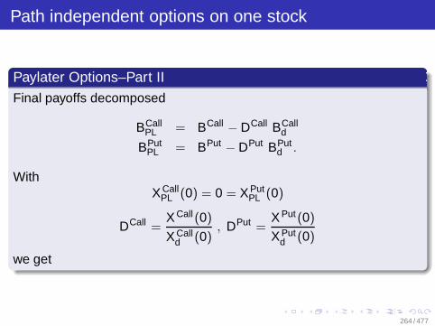
Path independent options on one stock
Paylater Options–Part IIFinal payoffs decomposed
BCallPL = BCall − DCall BCall
d
BPutPL = BPut − DPut BPut
d .
WithX Call
PL (0) = 0 = X PutPL (0)
DCall =X Call(0)
X Calld (0)
, DPut =X Put(0)
X Putd (0)
we get
264 / 477

Path independent options on one stock
Paylater Options–Part III
X CallPL = P1(t)Φ(d1(t)) −
p1Φ(d1(0))
Φ(d2(0))Φ(d2(t)) ert
X PutPL = −P1(t)Φ(−d1(t)) +
p1Φ(−d1(0))
Φ(−d2(0))Φ(−d2(t)) ert
265 / 477
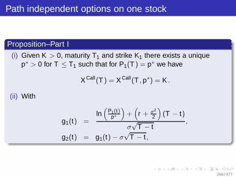
Path independent options on one stock
Proposition–Part I(i) Given K > 0, maturity T1 and strike K1 there exists a unique
p∗ > 0 for T ≤ T1 such that for P1(T ) = p∗ we have
X Call(T ) = X Call(T , p∗) = K .
(ii) With
g1(t) =ln(
P1(t)p∗
)+(
r + σ2
2
)(T − t)
σ√
T − t,
g2(t) = g1(t) − σ√
T − t ,
266 / 477

Path independent options on one stock
Proposition–Part II
h1(t) =ln(
P1(t)K1
)+(
r + σ2
2
)(T1 − t)
σ√
T1 − t,
h2(t) = h1(t) − σ√
T1 − t ,
we get the price of a call on a call
X CCcom(t) = P1(t)Φ
(ρ1)(g1(t), h1(t))
− K1e−r(T1−t)Φ(ρ1)(g2(t), h2(t))
− Ke−r(T−t)Φ(g2(t))
267 / 477
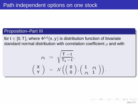
Path independent options on one stock
Proposition–Part III
for t ∈ [0, T ], where Φ(ρ)(x , y) is distribution function of bivariatestandard normal distribution with correlation coefficient ρ and with
ρ1 :=
√T − tT1 − t
,
(XY
)∼ N
((00
),
(1 ρ1
ρ1 1
)).
268 / 477
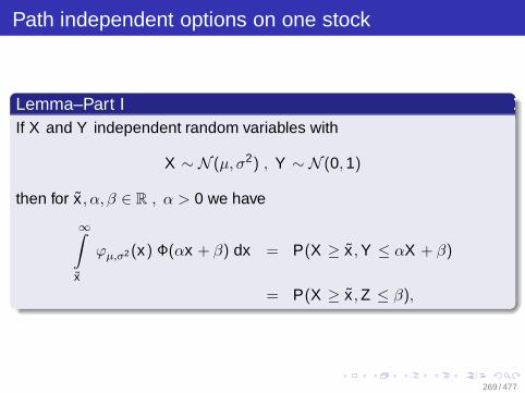
Path independent options on one stock
Lemma–Part IIf X and Y independent random variables with
X ∼ N (µ, σ2) , Y ∼ N (0, 1)
then for x , α, β ∈ R , α > 0 we have
∞∫
x
ϕµ,σ2(x) Φ(αx + β) dx = P(X ≥ x , Y ≤ αX + β)
= P(X ≥ x , Z ≤ β),
269 / 477

Path independent options on one stock
Lemma–Part IIwhere
(X , Z ) ∼ N((
µ−αµ
),
(σ2 −ασ2
−ασ2 1 + α2σ2
))
=⇒ ϕµ,σ2 is density function of the normal distribution with mean µ
and variance σ2.
270 / 477

Options on more than one underlying Stock
Indexed OptionsConsider 2-dimensional Black-Scholes model with given stock prices
dPi(t) = Pi (bi dt + σi1 dW1(t) + σi2 dW2(t)) ,
Pi(0) = pi (i = 1, 2)
Be a1, a2 ∈ R+. An indexed option with parameters a1, a2 is then given
by final payment
Bind = (a1P1(T ) − a2P2(T ))+ .
271 / 477
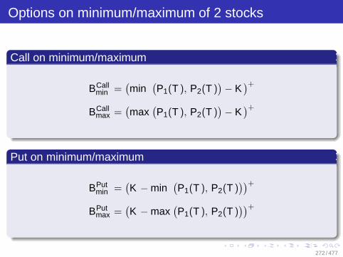
Options on minimum/maximum of 2 stocks
Call on minimum/maximum
BCallmin =
(min
(P1(T ), P2(T )
)− K
)+
BCallmax =
(max
(P1(T ), P2(T )
)− K
)+
Put on minimum/maximum
BPutmin =
(K − min
(P1(T ), P2(T )
))+
BPutmax =
(K − max
(P1(T ), P2(T )
))+
272 / 477

Options on minimum/maximum of 2 stocks
Proposition–Part IThe prices of the minimum/maximum options are given by
X Callmin (0) = p1Φ
(ρ) (d1, d3) + p2Φ(˜ρ) (d2, d4)
−Ke−rT Φ(ρ)(
d1 − σ1
√T , d2 − σ2
√T)
,
X Putmin (0) = X Call
min (0) + Ke−rT − p1Φ (d3) − p2Φ (d4) ,
X Callmax (0) = X Call
(1) (0) + X Call(2) (0) − X Call
min (0),
X Putmax (0) = X Put
(1) (0) + X Put(2) (0) − X Put
min (0),
273 / 477

Options on minimum/maximum of 2 stocks
Proposition–Part II
where X Call(i) , X Put
(i) denote prices of ordinary European calls/puts onstock i with strike K (i = 1, 2) and
σi :=√
σ2i1 + σ2
i2 (i = 1, 2),
ρ :=σ11σ21 + σ12σ22
σ1σ2,
ρ :=ρ σ2 − σ1
σ,
˜ρ :=ρσ1 − σ2
σ,
274 / 477

Options on minimum/maximum of 2 stocks
Proposition–Part III
di :=ln(pi
K
)+(r + 0.5σ2
i
)T
σi√
T,
di+2 :=(−1)i ln
(p1p2
)− 0.5σ2 T
σ√
T(i = 1, 2).
275 / 477

Path dependent options
One-sided barrier optionsOwner receives final payoff of European call/put if stock price does notexceed/does exceed given barrier before time T . Look atdown-and-out call and down-and-in call:
BCalldo = (P1(T ) − K )+ · 1P1(t)>b ∀ t∈[0,T ],
BCalldi = (P1(T ) − K )+ · 1∃ t∈[0,T ]: P1(t)≤b.
276 / 477
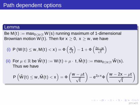
Path dependent options
LemmaBe M(t) := max0≤s≤t W (s) running maximum of 1-dimensionalBrownian motion W (t). Then for x ≥ 0, x ≥ w , we have
(i) P (W (t) ≤ w , M(t) < x) = Φ(
w√t
)− 1 + Φ
(2x−w√
t
)
(ii) For µ ∈ R be W (t) := W (t) + µ · t , M(t) := max0≤s≤t W (s).Thus we have
P(
W (t) ≤ w , M(t) < x)
= Φ
(w − µt√
t
)− e2µ xΦ
(w − 2x − µt√
t
)
277 / 477

Outline
4 Pricing of Exotic Options and Numerical AlgorithmsIntroductionExamplesExamplesEquivalent Martingale MeasureExotic Options with Explicit Pricing FormulaeWeak Convergence of Stochastic ProcessesMonte-Carlo SimulationApproximation via Binomial TreesThe Pathwise Binomial Approach of Rogers and Stapleton
278 / 477

General assumptions
General assumptions for this sectionWe consider the probability space
(Ω, F , P) = (C[0, 1], B(C[0, 1]), P),
i.e., the space of continuous, real-valued functions on [0,1] equippedwith the corresponding Borel σ-field and a probability measure P.
279 / 477

Stochastic process with distribution P
The function valued random variable X on (Ω, F , P) given by
X (ω) := ω, ω ∈ C[0, 1]
defines a real-valued stochastic process with distribution P.
Value of the process at time t ∈ [0, 1]:
X (t , ω) := πt X (ω) := ω(t).
→ projection on the "t-th coordinate" of ω.
280 / 477
Notion of convergence
The notion of convergence of stochastic process Xn via the usualweak convergence of random variables
Xn(t)n→∞−−−→ X (t) for all t ∈ [0, 1] in distribution
is too weak.
⇒ Consider weak convergence of probability measureson metric spaces
281 / 477
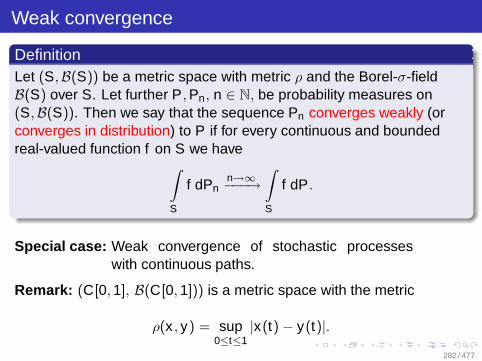
Weak convergence
DefinitionLet (S,B(S)) be a metric space with metric ρ and the Borel-σ-fieldB(S) over S. Let further P, Pn, n ∈ N, be probability measures on(S,B(S)). Then we say that the sequence Pn converges weakly (orconverges in distribution) to P if for every continuous and boundedreal-valued function f on S we have
∫
S
f dPnn→∞−−−→
∫
S
f dP.
Special case: Weak convergence of stochastic processeswith continuous paths.
Remark: (C[0, 1], B(C[0, 1])) is a metric space with the metric
ρ(x , y) = sup0≤t≤1
|x(t) − y(t)|.282 / 477

Weak convergence
DefinitionThe sequence of continuous stochastic processes Xn(t)t∈[0,1]
converges weakly (or in distribution) to X if for all f ∈ C(C[0, 1], R) wehave
Ef (Xn)n→∞−−−→ Ef (X ).
Remark: C(C[0, 1], R) is the space of the uniformly continuous,bounded functionals on C[0, 1].
283 / 477
Weak convergence
Stochastic process Xn is defined on (C[0, 1], B(C[0, 1]), Pn).
Process X is defined on (C[0, 1], B(C[0, 1]), P).
P, Pn are probability measures on (C[0, 1], B(C[0, 1])).
Ef (Xn) =∫
f (Xn) dP =∫
f dPnn→∞−−−→
∫f dP =
∫f (X ) dP = Ef (X ).
⇒ The weak convergence of stochastic processesis represented as the weak convergence of theprobability measures Pn → P.
284 / 477

Weak convergence
TheoremLet P, Pn, n ∈ N, be probability measures on the metric space(S,B(S)) endowed with the metric ρ. Further, let h : S → S′ be ameasurable mapping into a metric space S′ with metric ρ′ andBorel-σ-field B(S′). If for the set Dh of points of discontinuity of h wehave
P(Dh) = 0,
then we get
Pnn→∞−−−→ P in distribution ⇒ Pn · h−1 n→∞−−−→ P · h−1 in distribution.
⇒ Weak convergence is preserved under continuous mappings.
285 / 477
Weak convergence
CorollaryIf the sequence Xn of continuous stochastic processes convergesweakly to the continuous process X, then for every fixed t ∈ [0, 1] therandom variables Xn(t) converge in distribution to X (t).
286 / 477
Weak convergence
RemarkDefine the projections
πt1,...,tk : C[0, 1] → Rk
byπt1,...,tk (ω) = (ω(t1), . . . , ω(tk ))
for 0 ≤ t1 < . . . < tk ≤ 1. Then, we have
Xnn→∞−−−→ X in distribution
⇒ (Xn(t1), . . . , Xn(tk ))n→∞−−−→ (X (t1), . . . , X (tk )) in distribution.
287 / 477
Weak convergence
RemarkWeak convergence of stochastic processes implies convergenceof the finite-dimensional distributions.
Convergence of all finite-dimensional distributions
Pn · π−1t1,...,tk
does not in general imply convergence of the distributions Pn ofthe corresponding processes.
If the sequence of the Pn is relatively compact (i.e., eachsubsequence contains a weakly convergent subsequence), thenthe convergence of the finite-dimensional subsequences impliesweak convergence of the Pn.
288 / 477

Approximation of the one-dimensional Brownianmotion
Algorithm
(1) Choose a sequence ξnn∈N of i.i.d. random variables of a simpleform with
E(ξi) = 0, Var(ξi) = σ2 < ∞and set
S0 := 0, Sn :=n∑
i=1
ξi .
Example: ξi = Yi − q with Yi ∼ B(1, q).
289 / 477

Approximation of the one-dimensional Brownianmotion
Algorithm(2) By means of linear interpolation construct a stochastic process
Xn(t) with continuous paths of that sequence
Xn(t , ω) =1
σ√
nS[nt](ω) + (nt − [nt])
1σ√
nξ[nt]+1(ω)
for t ∈ [0, 1], n ∈ N, i.e., we have
Xn( k
n , ω)
=1
σ√
nSk(ω),
and for t ∈(k
n , k+1n
)we obtain Xn(t) by linear interpolation.
290 / 477
Approximation of the one-dimensional Brownianmotion
Algorithm(3) The finite-dimensional distributions of Xn converge in distribution
to that of a Brownian motion.
• From [ns]n
n→∞−−−→ s and the central limit theorem, we obtain
1σ√
nS[ns]
n→∞−−−→ W (s) in distribution.
• Chebychev’s inequality yields∣∣∣∣Xn(s) − 1
σ√
nS[ns]
∣∣∣∣ ≤1
σ√
n|ξ[ns]+1| n→∞−−−→ 0 in probability.
Hence,Xn(s)
n→∞−−−→ W (s) in distribution.
291 / 477

Approximation of the one-dimensional Brownianmotion
Algorithm• Due to the independence of the ξi and the theorem of Slut-
sky this results in(
1σ√
nS[ns],
1σ√
n
(S[nt] − S[ns]
)) n→∞−−−→ (Ws, Wt − Ws)
for s < t . From this we get
(Xn(s), Xn(t) − Xn(s))n→∞−−−→ (Ws, Wt − Ws) in distribution.
Slutsky’s theorem implies
(Xn(s), Xn(t))n→∞−−−→ (Ws, Wt) in distribution.
Analogously: Convergence of finite tuples ofXn(ti)-components.
292 / 477

Approximation of the one-dimensional Brownianmotion
Algorithm(4) Show that the sequence of the distributions Pn on
(C[0, 1], B(C[0, 1])) corresponding to Xn is relatively compact.
293 / 477

Donsker’s theorem
Donsker’s theoremLet ξnn∈N be an i.i.d. sequence with
E(ξi) = 0 and 0 < Var(ξi) = σ2 < ∞.
Then, the sequence Xn of stochastic processes defined by
Xn(t , ω) =1
σ√
nS[nt](ω) + (nt − [nt])
1σ√
nξ[nt]+1(ω), t ∈ [0, 1], n ∈ N
converges weakly to the one-dimensional Brownian motionW (t), t ∈ [0, 1].
294 / 477
Donsker’s theorem
RemarkThe convergence assertion and the limiting distribution areindependent of the exact choice of ξi
(Donsker’s invariance principle).
Donsker’s theorem can be viewed as the "process version" of thecentral limit theorem.
Donsker’s theorem can be assumed valid for arbitrary intervals[0, T ].
295 / 477

Donsker’s theorem for triangular schemes
Donsker’s theorem for triangular schemesThe random variables ξn1, . . . , ξnkn
, n ∈ N, kn ∈ N, are assumed to bei.i.d. with E(ξn1) = 0 and 0 < Var(ξn1) = σ2
n1≤ c, where c > 0. Let
Sni:= ξn1 + . . . + ξni , 1 ≤ i ≤ kn,
s2ni
:= σ2n1
+ . . . + σ2ni
= i · σ2n1
,
s2n := s2
nkn= kn · σ2
n1.
Define the process Xn(t), t ∈ [0, 1], by
Xn(0) := 0,
Xn
(s2
ni/s2n
):= Sni/sn , i = 1, . . . , kn,
and via linear interpolation on the intervals[s2
ni−1/s2
n, s2ni
/s2n
].
If kn → ∞ and sn → ∞ for n → ∞, then Xn converges weakly to theBrownian motion W .
296 / 477

Donsker’s theorem
RemarkWe have
E(h(Xn))n→∞−−−→ E(h(X ))
for continuous and bounded functionals h : C[0, T ] → R.
Not sufficient for practical applications.
If in the Black-Scholes model we approximate the Brownianmotion by a sequence of processes Xn, Donsker’s theorem wouldnot directly imply
E(
eb·T+σ·Xn(T ))
n→∞−−−→ E(
eb·T+σ·W (T ))
as the exponential functional is not bounded.
Additionally, we need the uniform integrability of the sequenceexp(σXn(t)).
297 / 477
Weak convergence
TheoremLet the sequence of random variables Xnn∈N be uniformly integrable.Assume further that we have
Xnn→∞−−−→ X in distribution.
Then this impliesE(Xn)
n→∞−−−→ E(X ).
298 / 477
Outline
4 Pricing of Exotic Options and Numerical AlgorithmsIntroductionExamplesExamplesEquivalent Martingale MeasureExotic Options with Explicit Pricing FormulaeWeak Convergence of Stochastic ProcessesMonte-Carlo SimulationApproximation via Binomial TreesThe Pathwise Binomial Approach of Rogers and Stapleton
299 / 477
The basic idea
Description of the idea
The basis of Monte-Carlo simulation is the strong law of largenumbers
⇒ Arithmetic mean of independent, identically distributed ran-dom variables converges towards their mean almost surely.
Computing an option price = Computing the discountedexpectation (with respect to the equivalent martingale measure) ofthe payoff B.
300 / 477
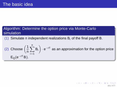
The basic idea
Algorithm: Determine the option price via Monte-Carlosimulation(1) Simulate n independent realizations Bi of the final payoff B.
(2) Choose(
1n
n∑
i=1
Bi
)· e−rT as an approximation for the option price
EQ(e−rT B).
301 / 477

Simulation of the payoff B
Assume that the payment B is a functional of the price processP1(t), t ∈ [0, T ].
Simulate a path P1(t) of the stock price process with respect tothe equivalent martingale measure Q.
A path can only be simulated approximately (it is given by infinitelymany values).
302 / 477

Simulation of the payoff B
Procedure(1) Divide the interval [0, T ] into N ≫ 1 equidistant parts.
(2) Generate N independent random numbers Yi which areN (0, 1)-distributed.
(3) From those, simulate an (approximate) path W (t) of the Brownianmotion on [0, T ]:
W (0) = 0,
W(j · T
N
)= W
((j − 1) · T
N
)+√
TN · Yj , j = 1, . . . , N,
W (t) = W((j − 1) · T
N
)
+ (t − (j − 1) · TN ) · N
T ·[W(j · T
N
)− W
((j − 1) · T
N
)],
for t ∈[(j − 1) · T
N , j · TN
]
303 / 477

Simulation of the payoff B
Procedure(4) Use this to generate an (approximate) path of the price process
P1(t):
P1(t) = p1 · e(
r−12 σ2)
t · eσ·W (t), t ∈ [0, T ].
(5) With this simulated path of the price process compute an estimatefor the payoff B.
Example (European call): Bi = (P1(T ) − K )+.
304 / 477

Simulation of the payoff B
RemarkFor the practical realization of the computation of Bi in step 5 it oftenproves to be more convenient to do the interpolation in step 4 and notin step 3:
P1(0) = p1,
P1(j · T
N
)= P1
((j − 1) · T
N
)· e(
r−12 σ2) T
N · eσ·√
TN ·Yj
, j = 1, . . . , N,
P1(t) = P1((j − 1) · T
N
)
+ (t − (j − 1) · TN ) · N
T ·[P1(j · T
N
)− P1
((j − 1) · T
N
)],
for t ∈[(j − 1) · T
N , j · TN
].
For large N the differences between both methods are negligible.
305 / 477
Convergence of the method
Let P(N)1 (t), t ∈ [0, T ] be the approximate price process.
If B is a continuous and bounded functional on C([0, T ]) then byDonsker’s theorem we have the convergence
EQ
(B(
P(N)1 (t), t ∈ [0, T ]
))N→∞−−−−→ EQ
(B(P1(t), t ∈ [0, T ])
).
If B is a continuous functional on C([0, T ]), then the convergenceof the option price is guaranteed if the family
B(
P(N)1 (t), t ∈ [0, T ]
) ∣∣∣∣N ∈ N
is uniformly integrable.
306 / 477

Convergence of the method
Showing the uniformly integrability can be tricky for specificchoices of B. Then for a given N the expected value
EQ
(B(
P(N)1 (t), t ∈ [0, T ]
))
will be approximated by the arithmetic mean
1n
n∑
i=1
B(
P(N)1,i (t), t ∈ [0, T ]
)
by the strong law of large numbers. Here, P(N)1,i (t) are different
paths which have been generated according to the aboveprocedure.
307 / 477

Advantages/Disadvantages of the Monte-Carlo method
Advantages
Easy to implement.
Reasonable number generators are available.
Every exotic option can be approximated.
Refinements to obtain faster convergence are available.
Disadvantages
Method is time-consuming (n and N have to be very large).
Frequently n and N have to be so large that the whole reservoir ofpseudo-random numbers is used and an already used sequenceof pseudo-random numbers has to be reused (→ independenceassumption of the different simulations is no longer true).
Strong dependence of the method on the quality of the randomnumber generator.
308 / 477
Outline
4 Pricing of Exotic Options and Numerical AlgorithmsIntroductionExamplesExamplesEquivalent Martingale MeasureExotic Options with Explicit Pricing FormulaeWeak Convergence of Stochastic ProcessesMonte-Carlo SimulationApproximation via Binomial TreesThe Pathwise Binomial Approach of Rogers and Stapleton
309 / 477

The basic idea
Description of the idea
Monte-Carlo simulation relies on the strong law of large numbers.
The approximation method via binomial trees can be motivated bythe central limit theorem.
310 / 477

Cox-Ross-Rubinstein model
Stock price process: P(n)1 (i), i = 0, 1, . . . , n
Possible paths given by binomial tree→ price process starts in p at time t = 0→ in each node the price P(n)
1 (i) can increaseby the factor u with probability q orby the factor d with probability (1 − q) (where d < u).
The probability of a price increase by the factor u and the possiblevalues of the relative price change
P(n)1 (i)
P(n)1 (i − 1)
are the same in each node.The factors u and d satisfy
d < er∆t < u with ∆t :=Tn
.
→ avoid riskless gains311 / 477
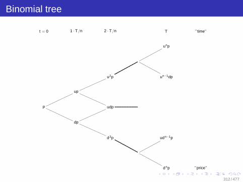
Binomial tree
t = 0 1 · T/n 2 · T/n T ”time”
unpppppppppppppppp
NNNNNNNNNNNNNN
u2p un−1dp
up
mmmmmmmmmmmmmmmm
QQQQQQQQQQQQQQQQ
p
nnnnnnnnnnnnnnnnn
PPPPPPPPPPPPPPPPP udp
dp
mmmmmmmmmmmmmmmm
QQQQQQQQQQQQQQQQ
d2p udn−1ppppppppppppppp
NNNNNNNNNNNNNNN
dnp ”price”
312 / 477
Cox-Ross-Rubinstein model
Number of "up-moves" of P(n)1 (i): Xn
Properties:Xn ∼ B(n, q)
P(n)1 (n) = p · uXn · dn−Xn = p · eXn·ln(u/d)+n·ln(d).
313 / 477

Cox-Ross-Rubinstein model
Special case:
q =12
, b ∈ R
and
u = eb∆t+σ√
∆t , d = eb∆t−σ√
∆t
b =12
ln(u) + ln(d)
∆t, σ =
12
ln(u) − ln(d)
∆t
Convergence:
P(n)1 (n) = p · exp
(b · T + σ
√T(
2Xn − n√n
))
n→∞−−−→ p · exp(
b · T + σ · W (T )
)= P1(T ) in distribution
314 / 477

Cox-Ross-Rubinstein model
Note that2Xn − n√
n
has zero mean and variance 1.2Xn is the sum of n independent, double Bernoulli variables.Important: Convergence of the discrete to the continuous priceprocess.Discounted expected payoff of the option in the discrete modelcan be computed easily.With increasing degree of fineness of the time discretization, thediscounted expected final payment in the discrete-time model willconverge to that of the continuous-time model if the family
Bn := B(
P(n)1 (i), i = 0, 1, . . . , n
)
is uniformly integrable.315 / 477
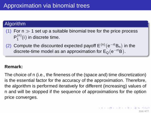
Approximation via binomial trees
Algorithm(1) For n ≫ 1 set up a suitable binomial tree for the price process
P(n)1 (i) in discrete time.
(2) Compute the discounted expected payoff E (n)(e−rtBn
)in the
discrete-time model as an approximation for EQ(e−rtB
).
Remark:
The choice of n (i.e., the fineness of the (space and) time discretization)is the essential factor for the accuracy of the approximation. Therefore,the algorithm is performed iteratively for different (increasing) values ofn and will be stopped if the sequence of approximations for the optionprice converges.
316 / 477

Choice of parameters in the binomial trees
Independence of the identically distributed increments
P(n)1 (i)
P(n)1 (i − 1)
in the binomial tree implies weak convergence of
P(n)
1 (i), i = 0, 1, . . . , n
to
P1(t), t ∈ [0, T ]
if the first two moments of the logarithm of increments
ln(
P(n)1 (i)
P(n)1 (i − 1)
)and ln
(P1(i · T
n )
P1((i − 1) · T
n
))
of the discrete and continuous price processes coincide at times i · Tn .
317 / 477
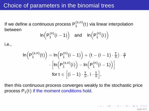
Choice of parameters in the binomial trees
If we define a continuous process P(s,n)1 (t) via linear interpolation
betweenln(
P(n)1 (i − 1)
)and ln
(P(n)
1 (i))
i.e.,
ln(
P(s,n)1 (t)
)= ln
(P(n)
1 (i − 1))
+(t − (i − 1) · T
n
)· n
T
·[ln(
P(s,n)1 (i)
)− ln
(P(n)
1 (i − 1))]
for t ∈[(i − 1) · T
n , i · Tn
],
then this continuous process converges weakly to the stochastic priceprocess P1(t) if the moment conditions hold.
318 / 477

Choice of parameters in the binomial trees
Consider the price process with respect to the equivalentmartingale measure Q and assume that
P1(t)P0(t)
is a martingale.
Binomial measure with respect to time discretization n: Q(n).
Expectation with respect to that measure: E (n).F (n)
i
i∈0,1,...,n filtration generated by the price process
P(n)
1 (i)
i∈0,1,...,n.
319 / 477
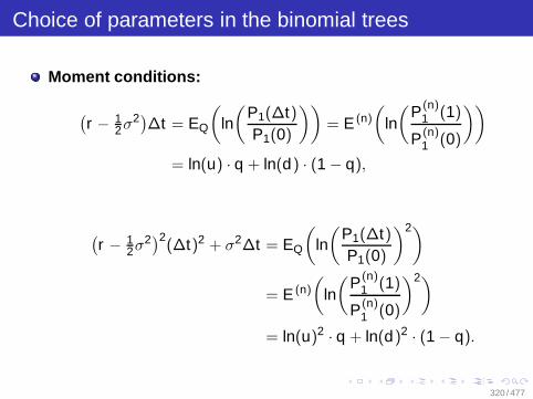
Choice of parameters in the binomial trees
Moment conditions:
(r − 1
2σ2)∆t = EQ
(ln(
P1(∆t)P1(0)
))= E (n)
(ln(
P(n)1 (1)
P(n)1 (0)
))
= ln(u) · q + ln(d) · (1 − q),
(r − 1
2σ2)2(∆t)2 + σ2∆t = EQ
(ln(
P1(∆t)P1(0)
)2)
= E (n)
(ln(
P(n)1 (1)
P(n)1 (0)
)2)
= ln(u)2 · q + ln(d)2 · (1 − q).
320 / 477

Choice of parameters in the binomial trees
Moment conditions:
(r − 1
2σ2)∆t = EQ
(ln(
P1(∆t)P1(0)
))= E (n)
(ln(
P(n)1 (1)
P(n)1 (0)
))
= ln(u) · q + ln(d) · (1 − q),
(r − 1
2σ2)2(∆t)2 + σ2∆t = EQ
(ln(
P1(∆t)P1(0)
)2)
= E (n)
(ln(
P(n)1 (1)
P(n)1 (0)
)2)
= ln(u)2 · q + ln(d)2 · (1 − q).
321 / 477

Choice of parameters in the binomial trees
Unknown parameters:
u, d "incremental factors",
q "probability of an upwards movement"
Moment conditions allow free choice of one of the parameters if
u, d > 0 and q ∈ (0, 1).
Popular choices:
u =1d
, d < 1 or q =12
.
322 / 477

Choice of parameters in the binomial trees
Special case: q = 12
Moment conditions:
ln(u · d) = 2(r − 1
2σ2)∆t
ln(u)2 + ln(d)2 = 2(r − 1
2σ2)(∆t)2 + 2σ2∆t
Symmetric in u and d
Ansatz:u = eB+C , d = eB−C .
⇒ B =(r − 1
2σ2)∆t , C = |σ| ·
√∆t .
⇒ u = e(
r−12σ2)∆t+|σ|·
√∆t , d = e
(r−1
2σ2)∆t−|σ|·
√∆t .
323 / 477

Choice of parameters in the binomial trees
Special case: q = 12
For r > 0 we have
0 < d < u and d < er∆t .
To obtainer∆t < u
we must have|σ| ·
√∆t − 1
2σ2∆t > 0.
Time discretization must be sufficiently fine:
n >T · σ2
4.
324 / 477
The option price in the binomial model
The stock price model given by a binomial tree together with thepossibility of a bond investment at times i · T
n (with a bond priceP0(t) = ert ) constitute a complete market.
Price of an option = discounted expectation of the payoff B int = T with respect to the unique equivalent martingale measureQn.
Qn is given by the "upwards probability" q = qn.
325 / 477

The option price in the binomial model
For given u and d with
0 < d < er∆t < u
we obtain q from the martingale requirement
0 = EQn
(P(n)
1 (i)
P0(i · T
n
) − P(n)1 (i − 1)
P0((i − 1) · T
n
)∣∣∣∣F
(n)i−1
)
=P(n)
1 (i − 1)
P0((i − 1) · T
n
) ·(
(q · u + (1 − q) · d) e−r Tn − 1
)
as
q =er T
n − du − d
.
326 / 477
The option price in the binomial model
For given u and d with
u = e(
r−12 σ2)∆t+|σ|·
√∆t and d = e
(r−1
2σ2)∆t−|σ|·
√∆t
q differs from 1/2.
The value E (n)(e−rT Bn
)computed as an approximation for the
option priceEQ(e−rT B
)
in the continuous model will in general not coincide with the optionprice
EQn
(e−rT Bn
)
in the binomial model.
327 / 477

The option price in the binomial model
The use of binomial trees serves us only as a method ofnumerical approximation of the expectation EQ
(e−rT B
).
The fact that this expectation is an option price has no meaning forthe numerical method.
There is no reason why the approximating sequence for thisexpectation should be option prices in some discretized models.
328 / 477

The option price in the binomial model
Another method of approximation of EQ(e−rT B
)is to determine
q, u, d via requiring the equality of the first two moments of theincrements of the discrete- and the continuous-time price process.
Equality of the first moment of the increments with theindependence and identical distribution of all increments in thebinomial model imply the martingale condition.
Choose u, d such that the second moment of the increments ofboth price models coincide.
The option price in the binomial model (given by n, q, u, d ) iscomputed as an approximation for the option price in thecontinuous model.
329 / 477

The option price in the binomial model
The concept
"approximate the option price in the continuous model by thediscrete-time model option price"
cannot be justified by weak convergence arguments.
330 / 477
Computation of the expected discounted payoff in thebinomial tree
The possibility of an efficient calculation of the expectationE (n)
(e−rT Bn
)depends on the type of the functional B
(resp. its discretized variant Bn).
Two examples for n = 2:
European call
Double-barrier knockout call
331 / 477
Computation of the expected discounted payoff in thebinomial tree
The European call
Choose q = 12 and
market parameters r = 0, σ = 0.5, T = 2, p = 1.
332 / 477

Computation of the expected discounted payoff in thebinomial treeBinomial tree for P(2)
1 (i):
t = 0 1 2 ”time”
2.117
1.455
1/2nnnnnnnnnnnnn
1/2 PPPPPPPPPPPPP
1
1/2nnnnnnnnnnnnnnn
1/2 PPPPPPPPPPPPPPP 0.779
0.535
1/2nnnnnnnnnnnnn
1/2 PPPPPPPPPPPPP
0.287 ”price”
333 / 477

Computation of the expected discounted payoff in thebinomial tree
The European call
Aim: Value a European option with a payoff of the form
B = f (P1(T )).
Approximate its value by the two-period binomial tree and thediscretized variant of the payoff
B2 = f(P(2)
1 (2)).
Discounted expected payoff (discretized model)
E (2)(B2) =12
(12
[f (2.117) + f (0.779)
])
+12
(12
[f (0.779) + f (0.287)
])
334 / 477
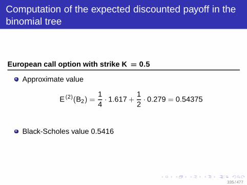
Computation of the expected discounted payoff in thebinomial tree
European call option with strike K = 0.5
Approximate value
E (2)(B2) =14· 1.617 +
12· 0.279 = 0.54375
Black-Scholes value 0.5416
335 / 477

Computation of the expected discounted payoff in thebinomial tree
Backwards induction principle
Payoff:B = f
(P1(T )
).
LetBn = f
(P(n)
1 (n))
and
V (n)(
i · Tn
, P(n)1 (i)
):= E (n)
(e−r(
T−i ·Tn)· Bn
∣∣∣P(n)1 (i)
)
be the expected payoff in t = T discounted back to t = i · Tn , if the
stock price in the binomial model at time t = i · Tn attains the value
P(n)1 (i).
336 / 477

Computation of the expected discounted payoff in thebinomial tree
Backwards induction principle
Expected discounted payoff of the option in the binomial model
V (n)(
T , P(n)1 (n)
)= f(P(n)
1 (n)),
V (n)(
i · Tn
, P(n)1 (i)
)
=12
[V (n)
((i + 1) · T
n, uP(n)
1 (i))
+ V (n)((i + 1) · T
n, dP(n)
1 (i))]
· e−r Tn , for i = n − 1, . . . , 0
E (n)(
e−rT Bn
)= V (n)(0, p).
337 / 477

Backwards induction principle
Advantage of the induction scheme:
Calculate onlyn · (n − 1)
2arithmetic means (although the stock price can follow 2n differentpaths).
Binomial tree = recombining tree
338 / 477

Backwards induction principle (modification)
How about path-dependent options?
In case of path-dependent options path dependency has to be takeninto account
⇒ Modification of backward induction recursion.
339 / 477

Backwards induction principle (modification)
Example: Double-barrier knockout call
Payoff:
BCallDB = (P1(T ) − 0.5)+ · 1
P1(t)∈[0.4, 1.4] for all t∈[0,T ]
Payoff (discrete):(
BCallDB
)2
=(P(2)
1 (2) − 0.5)+ · 1
P(2)1 (i)∈[0.4, 1.4], i=0,1,2
= 0.279 · 1P(2)
1 (2)=0.779, P(2)1 (1)=0.535
Double-barrier knockout call price (discrete approximation):
E (2)(B2) =14· 0.279 = 0.06975.
340 / 477
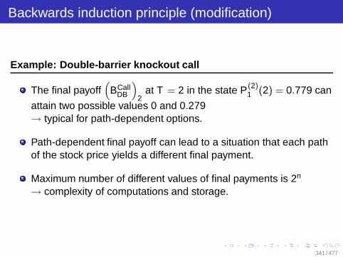
Backwards induction principle (modification)
Example: Double-barrier knockout call
The final payoff(
BCallDB
)2
at T = 2 in the state P(2)1 (2) = 0.779 can
attain two possible values 0 and 0.279→ typical for path-dependent options.
Path-dependent final payoff can lead to a situation that each pathof the stock price yields a different final payment.
Maximum number of different values of final payments is 2n
→ complexity of computations and storage.
341 / 477

Backwards induction principle (modification)A non-recombining tree:
t = 0 1 2 ”time”
2.117
1.455
1/2nnnnnnnnnnnnn
1/2 PPPPPPPPPPPPP
0.779
1
1/2
1/2
AAAA
AAAA
AAAA
AAAA
AAAA
0.779
0.535
1/2nnnnnnnnnnnnn
1/2 PPPPPPPPPPPPP
0.287 ”price”
342 / 477
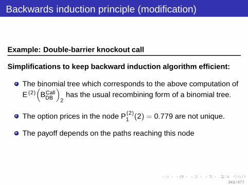
Backwards induction principle (modification)
Example: Double-barrier knockout call
Simplifications to keep backward induction algorithm effici ent:
The binomial tree which corresponds to the above computation of
E (2)(
BCallDB
)2
has the usual recombining form of a binomial tree.
The option prices in the node P(2)1 (2) = 0.779 are not unique.
The payoff depends on the paths reaching this node
343 / 477

Backwards induction principle (modification)
Principle of backward induction stays valid.
For a general path-dependent option we have to calculate up to2i−1 arithmetic means at time i (i + 1 in the non-path-dependentcase).
In the double-barrier knockout case, we can simply proceedbackwards in the recombining tree, but setting the option price tozero in all nodes where the knockout-condition is satisfied).
Computational complexity is comparable to that of a Europeannon-path-dependent option.
344 / 477

Backwards induction principle (modification)
In other cases such as
an average option with final payment of
BCallAv =
(1T
T∫
0
P1(t) dt − K)+
respectively its discrete variant
(BCall
Av
)n
=
(1
n + 1
n∑
i=0
P(n)1 (i) − K
)+
the full non-recombining tree has to be considered for theapproximative calculation of the option price.
345 / 477
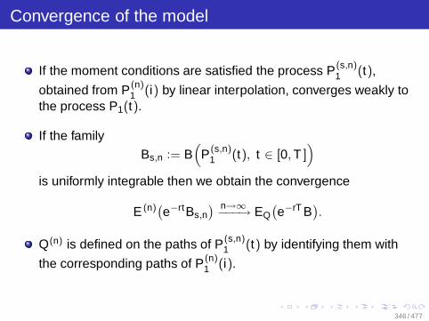
Convergence of the model
If the moment conditions are satisfied the process P(s,n)1 (t),
obtained from P(n)1 (i) by linear interpolation, converges weakly to
the process P1(t).
If the family
Bs,n := B(
P(s,n)1 (t), t ∈ [0, T ]
)
is uniformly integrable then we obtain the convergence
E (n)(e−rtBs,n
) n→∞−−−→ EQ(e−rT B
).
Q(n) is defined on the paths of P(s,n)1 (t) by identifying them with
the corresponding paths of P(n)1 (i).
346 / 477

Convergence of the model
We obtainE (n)
(e−rtBn
) n→∞−−−→ EQ(e−rT B
),
iflim
n→∞E (n)
(e−rt(Bs,n − Bn)
)= 0.
Remark: The latter convergence has to be proved for each type ofoption explicitly. It is satisfied if (Bs,n − Bn) converges to zero uniformly.
It is fulfilled for European lookbacks, barrier and double barrier options,and Asian options.
347 / 477

Advantages/Disadvantages of the method
Advantages
Easy to implement (but their efficiency can depend strongly on theoption type).
Binomial methods converge faster than Monte-Carlo-simulation.
Hybrid method via combination of binomial tree and Monte-Carlomethod for very big binomial trees available.
Disadvantages
Slow and irregular convergence behaviour for double barrieroptions.
Accuracy of approximation does not necessarily increase withfineness n.
348 / 477
Trinomial trees and explicit finite-difference methods
Option prices can be obtained as solutions of correspondingCauchy problems under certain assumptions.
In particular for options with a final payment of the form
B = f (P1(T )).
If the Cauchy problem does not admit an explicit solution we mustsolve it numerically.
Numerical methods: Connection between stochastic methods andPDE methods similar to Feynman-Kac theorem.
349 / 477
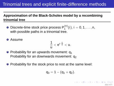
Trinomial trees and explicit finite-difference methods
Approximation of the Black-Scholes model by a recombiningtrinomial tree
Discrete-time stock price process P(n)1 (i), i = 0, 1, . . . , n,
with possible paths in a trinomial tree.
Assume1u
< er · Tn < u.
Probability for an upwards movement: q1
Probability for an downwards movement: q2
Probability for the stock price to rest at the same level:
q3 = 1 − (q1 + q2).
350 / 477

Trinomial trees and explicit finite-difference methodsTrinomial tree:
t = 0 1 · T/n 2 · T/n T ”time”
unp
u2p
rrrrrrrrrrrrrr un−1p
up
nnnnnnnnnnnnnnnnn
PPPPPPPPPPPPPPPPPP up up
p
ooooooooooooooooo
OOOOOOOOOOOOOOOOO p
nnnnnnnnnnnnnnnnnn
PPPPPPPPPPPPPPPPPPP p
1u p
nnnnnnnnnnnnnnnnnn
PPPPPPPPPPPPPPPP
1u2 p
rrrrrrrrrrrrrrrr
LLLLLLLLLLLLLL 1un−1 p
1un p ”price”
351 / 477

Trinomial trees and explicit finite-difference methods
Approximation of the Black-Scholes model by a recombiningtrinomial tree
Assume 0 < q1, q2 < 1, q1 + q2 ≤ 1.
q1 + q2 = 1 ⇒ binomial situationAssume: q1 + q2 < 1.
Donsker’s theorem ⇒ weak convergence of P(n)1 (i) to the stock
price process (in risk-neutral market)
P1(t) = p · exp((
r − 12
σ2)t + σW (t)),
if the first two moments of the increments of ln(P1(t)) between(i − 1) · T
n and i · Tn
ln(
P1(i · T
n
)
P1((i − 1) · T
n
))
coincide with the corresponding increments of ln(P(n)1 (i)).
352 / 477
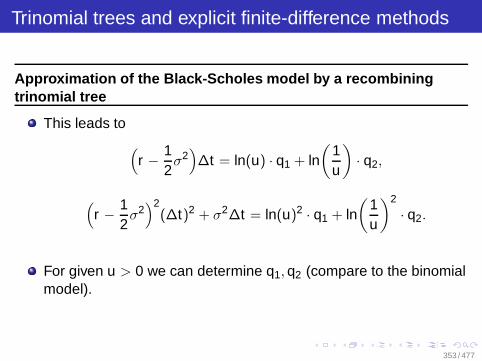
Trinomial trees and explicit finite-difference methods
Approximation of the Black-Scholes model by a recombiningtrinomial tree
This leads to
(r − 1
2σ2)∆t = ln(u) · q1 + ln
(1u
)· q2,
(r − 1
2σ2)2
(∆t)2 + σ2∆t = ln(u)2 · q1 + ln(
1u
)2
· q2.
For given u > 0 we can determine q1, q2 (compare to the binomialmodel).
353 / 477

Trinomial trees and explicit finite-difference methods
Approximation of the Black-Scholes model by a recombiningtrinomial tree
Method of Cox-Ross-Rubinstein:
u = eλσ√
∆t := e∆x
for some λ ∈ [1,∞) (neglect terms of higher order than ∆t above).
Error negligible for small ∆t .
λσ√
∆t(q1 − q2) =(r − 1
2σ2)∆t
λ2σ2∆t(q1 + q2) = σ2∆t .
354 / 477

Trinomial trees and explicit finite-difference methods
Approximation of the Black-Scholes model by a recombiningtrinomial tree
Solutions:
q1 =12
((r − 1
2σ2) 1
λσ
√∆t +
1λ2
),
q2 =12
(1λ2 −
(r − 1
2σ2) 1
λσ
√∆t)
.
q1, q2, q3 ∈ (0, 1) for small ∆t (i.e., large n).
λ = 1 ⇒ binomial model.
355 / 477
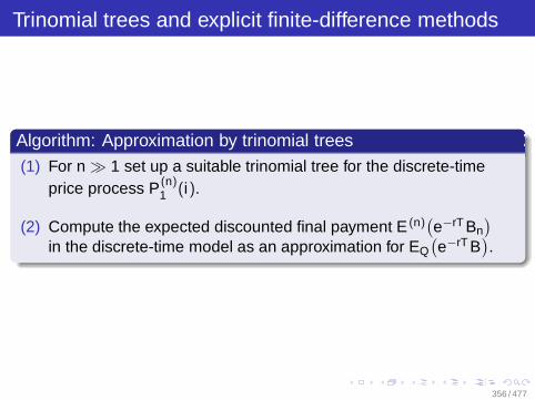
Trinomial trees and explicit finite-difference methods
Algorithm: Approximation by trinomial trees(1) For n ≫ 1 set up a suitable trinomial tree for the discrete-time
price process P(n)1 (i).
(2) Compute the expected discounted final payment E (n)(e−rT Bn
)
in the discrete-time model as an approximation for EQ(e−rT B
).
356 / 477

Computation of E (n)(e−rT Bn
)
Backward induction
LetX (n)
1 (i) := ln(P(n)
1 (i)), i = 0, 1, . . . , n,
and
V (n)(
i · ∆t , X (n)1 (i)
):= E (n)
(e−r(
T−i ·∆t)· Bn
∣∣∣P(n)1 (i)
)
357 / 477

Computation of E (n)(e−rT Bn
)
Backward induction
Compute recursively
V (n)(
T , X (n)1 (n)
)= f(
exp(X (n)
1 (n)))
,
V (n)(
i · ∆t , X (n)1 (i)
)
=
[q1V (n)
((i + 1) · ∆t , X (n)
1 (i) + ∆x)
+ q3V (n)((i + 1) · ∆t , X (n)
1 (i))
+ q2V (n)((i + 1) · ∆t , X (n)
1 (i) − ∆x)]
· e−r∆t ,
for i = n − 1, . . . , 0
E (n)(
e−rT Bn
)= V (n)(0, p).
358 / 477

The option price in the trinomial model
In general the final payment of a European call cannot bereplicated by a trading strategy in stock and bond in the trinomialmodel.
For this model exists a whole family of equivalent martingalemeasures.
The alternative method
"compute the option price in an approximating model"
cannot be performed without further modifications.
Until now we have not developed a method to compute an optionprice in incomplete markets.
359 / 477

Relations between trinomial trees and explicitfinite-difference methods
The option price solves the Cauchy problem
Vt +12
σ2p2Vpp + rpVp − rV = 0, (t , p) ∈ [0, T ] × (0,∞)
V (T , p) = f (p), p > 0.
Substitution:x = ln(p).
Notation:V (t , x) := V (t , p).
Transformed problem:
Vt +12σ2Vxx +
(r − 1
2σ2)Vx − r V = 0, (t , p) ∈ [0, T ] × R
V (T , x) = f (ex), x ∈ R.
360 / 477

Explicit finite-difference method
Time discretization: 0, ∆t , 2∆t , . . . , T
Space discretization: ln(p1), ln(p1) ± ∆x , ln(p1) ± 2∆x , . . .
∆t V (n)(t , x) :=V (n)(t + ∆t , x) − V (n)(t , x)
∆t,
∆x V (n)(t , x) :=V (n)(t + ∆t , x + ∆x) − V (n)(t + ∆t , x − ∆x)
2∆x,
∆xx V (n)(t , x)
:=V (n)(t + ∆t , x + ∆x) − 2V (n)(t + ∆t , x) + V (n)(t + ∆t , x − ∆x)
(∆x)2 .
361 / 477

Explicit finite-difference method
Notation:
ti := i · ∆t , i = 0, 1, . . . , n,
X (j) := ln(p1) + j · ∆x , j ∈ Z.
V (n)(ti , X (j))
=1
1 + r∆t
(12
σ2 ∆t(∆x)2 +
12
(r − σ2
2
)∆t∆x
)V (n)(ti + ∆t , X (j) + ∆x)
+
(1 − σ2 ∆t
(∆x)2
)V (n)(ti + ∆t , X (j))
+
(12σ2 ∆t
(∆x)2 +12
(r − σ2
2
)∆t∆x
)V (n)(ti + ∆t , X (j) − ∆x)
.
362 / 477

Explicit finite-difference method
At time T we know all values of V (n)(T , x).We obtain
V (n)(T − ∆t , X (j))
from the explicit representation.Via backward induction with step size ∆t we reach the startingtime t = 0 in n steps and obtain
V (n)(0, x)
as an approximation for the option price V (0, x).The recursion in the trinomial tree can be seen as a finitedifference scheme.V (n)(0, x) converges to V (0, x) if the stability condition
0 <∆t
(∆x)2 ≤ 1σ2
is satisfied.363 / 477

Outline
4 Pricing of Exotic Options and Numerical AlgorithmsIntroductionExamplesExamplesEquivalent Martingale MeasureExotic Options with Explicit Pricing FormulaeWeak Convergence of Stochastic ProcessesMonte-Carlo SimulationApproximation via Binomial TreesThe Pathwise Binomial Approach of Rogers and Stapleton
364 / 477

The pathwise binomial approach of Rogers andStapleton
Description of the basic idea
Binomial method: Only the distribution of P1(t) is approximated bya simpler, discrete distribution.
Method of Rogers and Stapleton: Approximate each single path ofP1(t) by a step function.
365 / 477
Description of the basic idea (continued)
The step function is only allowed to attain values in a givendiscrete set and should at most deviate by a given accuracy ε fromthe corresponding path of P1(t).
Idea: Interprete the set of all paths of a step function as an infinitebinomial tree.
Compute the (approximate) discounted expected payment of anoption in the infinite tree as an approximation for the option pricein the Black-Scholes model.
366 / 477

The pathwise binomial approach of Rogers andStapleton
Algorithm: Pathwise binomial approach of Rogers and Stapleton
(1) For a given accuracy ∆y and starting point y = ln(p1) set up aninfinite binomial tree.
(2) Compute the discounted payoff E (∆y)(e−rT B∆y
)of the option in
the infinite binomial tree as an approximation for EQ(e−rT B
).
367 / 477
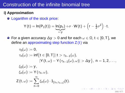
Construction of the infinite binomial tree
i) Approximation
Logarithm of the stock price:
Y (t) = ln(P1(t)) = ln(p1)︸ ︷︷ ︸=:y
+σ · W (t) +(
r − 12σ2)· t .
For a given accuracy ∆y > 0 and for each ω ∈ Ω, t ∈ [0, T ], wedefine an approximating step function Z (t) via
τ0(ω) := 0,
τn(ω) := inf
t ∈ [0, T ] | t > τn−1(ω),
|Y (t , ω) − Y (τn−1(ω), ω)| > ∆y, n = 1, 2, . . . ,
ξ0(ω) := y ,
ξn(ω) := Y (τn, ω),
Z (t , ω) :=∞∑
n=0
ξn(ω) · 1[τn,τn+1)(t).
368 / 477
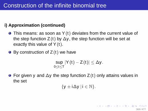
Construction of the infinite binomial tree
i) Approximation (continued)
This means: as soon as Y (t) deviates from the current value ofthe step function Z (t) by ∆y , the step function will be set atexactly this value of Y (t).
By construction of Z (t) we have
sup0≤t≤T
|Y (t) − Z (t)| ≤ ∆y .
For given y and ∆y the step function Z (t) only attains values inthe set
y ± i∆y | i ∈ N.
369 / 477

Construction of the infinite binomial tree
i) Approximation (continued)
Z (t) can only jump to adjacent values Z (t) ± ∆y
y−2∆
y−∆
y
y+∆
y+2∆
τ1
τ2
τ3 τ
4τ
5τ
6τ
7
Y(t),Z(t)
t
370 / 477

Construction of the infinite binomial tree
i) Approximation (continued)There is no a priori upper bound for the number of values thatZ (t , ω) can attain on [0, T ].
⇒ Identify the sequence of values of the step function Z (t , ω)on [0, T ] with a finite path in the infinite binomial tree.
y + 3∆y
y + 2∆yjjjj
TTTTT
y + ∆yjjjj
TTTTTTTTy + ∆y
yooooo
OOOOO yjjjjjjjjj
TTTTTTTTT . . .
y − ∆y
jjjjjjjj
TTTTy − ∆y
y − 2∆y
jjjjj
TTTT
y − 3∆y371 / 477
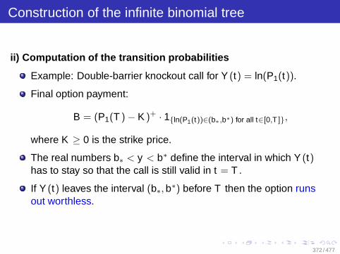
Construction of the infinite binomial tree
ii) Computation of the transition probabilities
Example: Double-barrier knockout call for Y (t) = ln(P1(t)).
Final option payment:
B = (P1(T ) − K )+ · 1ln(P1(t))∈(b∗ ,b∗) for all t∈[0,T ],
where K ≥ 0 is the strike price.
The real numbers b∗ < y < b∗ define the interval in which Y (t)has to stay so that the call is still valid in t = T .
If Y (t) leaves the interval (b∗, b∗) before T then the option runsout worthless.
372 / 477
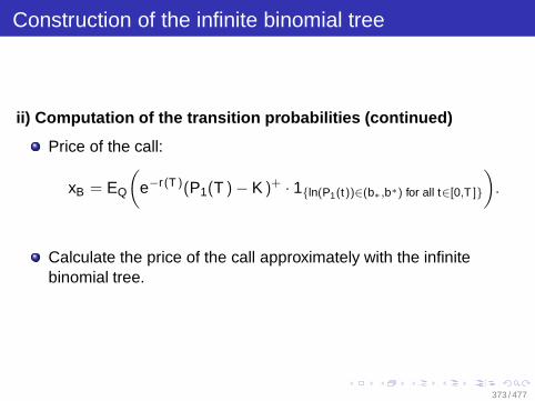
Construction of the infinite binomial tree
ii) Computation of the transition probabilities (continue d)
Price of the call:
xB = EQ
(e−r(T )(P1(T ) − K )+ · 1ln(P1(t))∈(b∗ ,b∗) for all t∈[0,T ]
).
Calculate the price of the call approximately with the infinitebinomial tree.
373 / 477
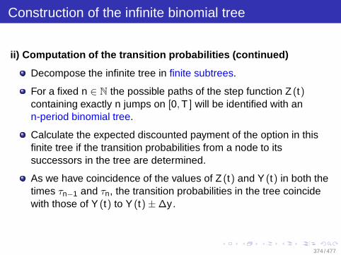
Construction of the infinite binomial tree
ii) Computation of the transition probabilities (continue d)
Decompose the infinite tree in finite subtrees.
For a fixed n ∈ N the possible paths of the step function Z (t)containing exactly n jumps on [0, T ] will be identified with ann-period binomial tree.
Calculate the expected discounted payment of the option in thisfinite tree if the transition probabilities from a node to itssuccessors in the tree are determined.
As we have coincidence of the values of Z (t) and Y (t) in both thetimes τn−1 and τn, the transition probabilities in the tree coincidewith those of Y (t) to Y (t) ± ∆y .
374 / 477

The pathwise binomial approach of Rogers andStapleton
TheoremFor a given ∆y > 0 the probability for an upwards movement of Z (t) inτn, n ∈ N, is given by
q =s(0) − s(−∆y)
s(∆y) − s(−∆y)
with
s(x) = −e−2cx and c =r − 1
2σ2
σ2 .
The probability for a downwards movement of Z (t) in τn, n ∈ N, is
(1 − q).
375 / 477

Continuation: Double-barrier knockout call
For the double-barrier knockout call all paths in the tree whichexceed b∗ by below and b∗ by above have zero value.
If the process Z (t) differs from b∗ or b∗ by a value less than ∆ywe have to take extra care.
To prevent the option being knocked out by the Y (.)-processbefore it is knocked out by the Z (.)-process, we must modify thedefinition of the Z (.)-process.
376 / 477
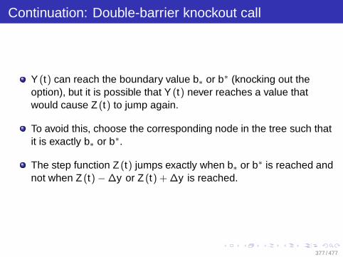
Continuation: Double-barrier knockout call
Y (t) can reach the boundary value b∗ or b∗ (knocking out theoption), but it is possible that Y (t) never reaches a value thatwould cause Z (t) to jump again.
To avoid this, choose the corresponding node in the tree such thatit is exactly b∗ or b∗.
The step function Z (t) jumps exactly when b∗ or b∗ is reached andnot when Z (t) − ∆y or Z (t) + ∆y is reached.
377 / 477
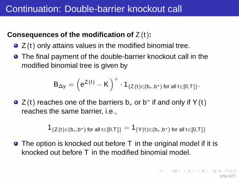
Continuation: Double-barrier knockout call
Consequences of the modification of Z (t):
Z (t) only attains values in the modified binomial tree.
The final payment of the double-barrier knockout call in themodified binomial tree is given by
B∆y =(
eZ (t) − K)+
· 1Z (t)∈(b∗,b∗) for all t∈[0,T ].
Z (t) reaches one of the barriers b∗ or b∗ if and only if Y (t)reaches the same barrier, i.e.,
1Z (t)∈(b∗,b∗) for all t∈[0,T ] = 1Y (t)∈(b∗ ,b∗) for all t∈[0,T ]
The option is knocked out before T in the original model if it isknocked out before T in the modified binomial model.
378 / 477

Continuation: Double-barrier knockout call
For the pricing of the knockout call, it plays no role if we defineZ (t) to be constant after reaching b∗ or b∗ or extend it as it wasoriginally defined.
It is important for the pricing purpose that the transitionprobabilities in the modified tree change for
Z (t) ∈ (b∗ − ∆y , b∗) or Z (t) ∈ (b∗, b∗ + ∆y).
379 / 477
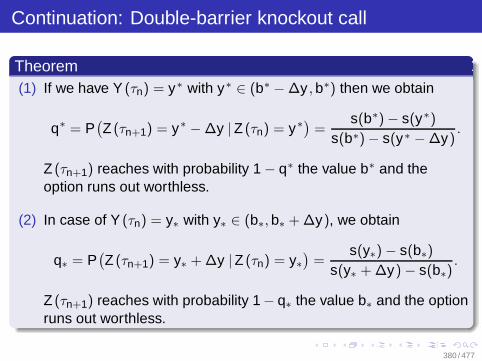
Continuation: Double-barrier knockout call
Theorem(1) If we have Y (τn) = y∗ with y∗ ∈ (b∗ − ∆y , b∗) then we obtain
q∗ = P(Z (τn+1) = y∗ − ∆y |Z (τn) = y∗) =
s(b∗) − s(y∗)s(b∗) − s(y∗ − ∆y)
.
Z (τn+1) reaches with probability 1 − q∗ the value b∗ and theoption runs out worthless.
(2) In case of Y (τn) = y∗ with y∗ ∈ (b∗, b∗ + ∆y), we obtain
q∗ = P(Z (τn+1) = y∗ + ∆y |Z (τn) = y∗
)=
s(y∗) − s(b∗)s(y∗ + ∆y) − s(b∗)
.
Z (τn+1) reaches with probability 1− q∗ the value b∗ and the optionruns out worthless.
380 / 477

Continuation: Double-barrier knockout call
PropositionLet Ψ(k , y) be the expected final payment of the option in the binomialmodel for an initial value of Z (0) = y ∈ (b∗, b∗) and a given numberk ∈ N ∪ 0 of upwards and downwards movements of Z (t) on [0, T ].Then Ψ(k , y) can be computed inductively according to the followingalgorithm
Ψ(0, y) = (ey − K )+
Ψ(n + 1, y) = q(y) · Ψ(n, y + ∆y) + q(y) · Ψ(n, y − ∆y), n = 0, 1, 2, . . .
381 / 477

Continuation: Double-barrier knockout call
Proposition (continued)Here the probabilities q(y) for y ∈ (b∗ + ∆y , b∗ − ∆y) are given by
q =s(0) − s(−∆y)
s(∆y) − s(−∆y)
with
s(x) = −e−2cx and c =r − 1
2σ2
σ2
and we haveq(y) = 1 − q(y).
382 / 477

Continuation: Double-barrier knockout call
Proposition (continued)For y ∈ (b∗, b∗ + ∆y) we have
q(y) = 0
and
q(y) =s(y) − s(b∗)
s(y + ∆y) − s(b∗).
For y ∈ (b∗ − ∆y , b∗) we have
q(y) = 0
and
q(y) =s(b∗) − s(y )
s(b∗) − s(y − ∆y).
383 / 477

Continuation: Double-barrier knockout call
Discounted expected final payment of the option in the modifiedbinomial tree:
E (∆y)(e−rT B∆y
)=
∞∑
n=0
P(v = n) · Ψ(n, y) · e−rT .
For the computation we need the probability distribution of thesum v of upwards and downwards movements of the stock pricein the binomial model.
Due toω | v(ω) ≥ n = ω | τn(ω) ≤ T
this distribution can be obtained from that of τn:
P(v = n) = P(v ≤ n) − P(v ≤ n − 1) = P(τn ≥ T ) − P(τn−1 ≥ T ).
384 / 477

Continuation: Double-barrier knockout call
Theorem(1) The random variables τn+1 − τnn∈N∪0 are independent and
identically distributed. Their Laplace transform ϕ(λ) is given by
ϕ(λ) = E(e−λτ1
)=
cosh(µσ−2∆y
)
cosh(γ∆y
)
with
µ = r − 12
σ2, γ =
√µ2 + 2λσ2
σ2 , λ > 0.
(2)E(τ1) =
∆yµ
· tanh(
µ
σ2 · ∆y)
for µ 6= 0,
E(τ21 ) = 2(E(τ1))
2 +σ2∆y
µ3 · tanh(
µ
σ2 ∆y)−(
∆yµ
)2
for µ 6= 0.
(3) τn+1 − τn is independent of ξn+1.
385 / 477

Continuation: Double-barrier knockout call
We have
τn =
n∑
i=1
(τi − τi−1).
Summands are independent and identically distributed.
Central limit theorem ⇒τn − n · E(τ1)√
n · Var(τ1)
n→∞−−−→ N(0, 1) in distribution.
Determine the distribution of τn approximately for large n.
For small n this approximation is not accurate enough.
386 / 477

Continuation: Double-barrier knockout call
TheoremWe have
P(
τn − n · E(τ1)√n · Var(τ1)
≤ x)
= Φ(x) +α3(1 − x2)e− x2
2√72πn
+ o(n−1
2)
with
α3 = E((
τ1 − E(τ1)√Var(τ1)
)3),
where Φ is the distribution function of the standard normal distribution.
387 / 477

Continuation: Double-barrier knockout call
Use Laplace transform ϕ(λ) to calculate α3:
α3 =∆y · (A + B − C)
(µσ2
)5σ6(s(∆y) − 1
)3 ,
A = 12 · µ
σ2 ∆y(s(2∆y) + s(∆y)
),
B = 8 ·( µ
σ2
)2(∆y)2(s(∆y) − s(2∆y)
),
C = 3 ·(1 + s(∆y) − s(2∆y) − s(3∆y)
).
388 / 477
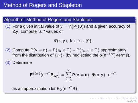
Method of Rogers and Stapleton
Algorithm: Method of Rogers and Stapleton
(1) For a given initial value of y = ln(P1(0)) and a given accuracy of∆y , compute "all" values of
Ψ(k , y), k ∈ N ∪ 0.
(2) Compute P(v = n) = P(τn ≥ T ) − P(τn−1 ≥ T ) approximatelyfrom the distribution of τnn (by neglecting the o
(n−1/2
)-terms).
(3) Determine
E (∆y)(e−rT B∆y
)=
∞∑
n=0
P(v = n) · Ψ(n, y) · e−rT
as an approximation for EQ(e−rT B
).
389 / 477
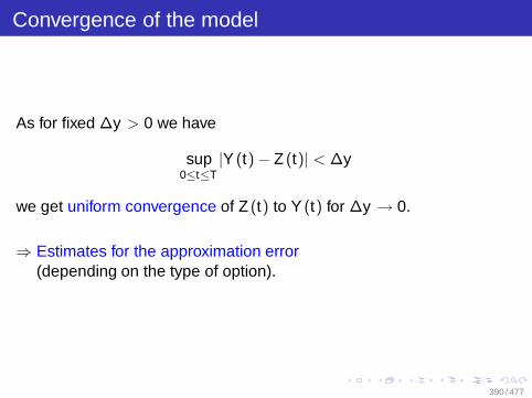
Convergence of the model
As for fixed ∆y > 0 we have
sup0≤t≤T
|Y (t) − Z (t)| < ∆y
we get uniform convergence of Z (t) to Y (t) for ∆y → 0.
⇒ Estimates for the approximation error(depending on the type of option).
390 / 477
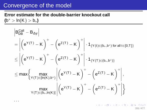
Convergence of the model
Error estimate for the double-barrier knockout call(b∗ > ln(K ) > b∗)
∣∣∣BCallDB − B∆y
∣∣∣
=
∣∣∣∣∣
(eY (T ) − K
)+
−(
eZ (T ) − K)+∣∣∣∣∣ · 1Y (t)∈(b∗ ,b∗) for all t∈[0,T ]
≤∣∣∣∣∣
(eY (T ) − K
)+
−(
eZ (T ) − K)+∣∣∣∣∣ · 1Y (T )∈(b∗,b∗)
≤ max
maxY (T )∈[ln(K ),b∗)
∣∣∣∣∣
(eY (T ) − K
)+
−(
eZ (T ) − K)+∣∣∣∣∣ ,
maxY (T )∈(b∗,ln(K )]
∣∣∣∣∣
(eY (T ) − K
)+
−(
eZ (T ) − K)+∣∣∣∣∣
. . .
391 / 477

Convergence of the model
Error estimate for the double-barrier knockout call(b∗ > ln(K ) > b∗)
∣∣∣BCallDB − B∆y
∣∣∣ ≤ . . .
≤ max(
eb∗ − eb∗−∆y)
, K · e∆y − K
= max
eb∗
(1 − e−∆y), K (e∆y − 1)
392 / 477

Advantages/Disadvantages of the method
Advantages
Paths of the approximating process Z (t) converge uniformly to thepaths Y (t) of the logarithm of the price process.
Explicit estimate of the convergence error.
Flexibility which allows for a choice of the nodes in the binomialtree ensuring that in the double-barrier knockout call case theoption runs out worthless in the modified binomial tree if and onlyif it runs out worthless in the Black-Scholes model.
Disadvantages
Concept requires a deeper understanding as in the case of thebinomial model.
Bigger computational complexity.
393 / 477

Outline
5 Optimal Portfolios
394 / 477

Outline
5 Optimal PortfoliosIntroduction and Formulation of the ProblemThe martingale methodOptimal Option PortfoliosExcursion 8: Stochastic ControlMaximize expected value in presence of quadratic control costsIntroductionPortfolio Optimization via Stochastic Control Method
395 / 477

Introduction
Until now
Trading strategies that generate a given payoff profile (replication)or a lower bound for a payment (hedging strategy).
Costs for replication strategy determined the price of the payoffprofile.
Now
Given a fixed initial capital and search for an admissibleself-financing pair of portfolio and consumption processes whichyields a payment stream as lucrative as possible.
396 / 477
Formulation of the portfolio problem
The continuous-time portfolio problem
Initial capital x > 0.
Determine an optimal consumption and investment strategy.
The investor has to determine
how many shares of which security he has to hold at which time instant
and
how much of his wealth he is allowed to consume
to maximize
his utility from consumption during the period [0, T ] and/orfrom the terminal wealth at the time horizon t = T .
397 / 477
Formulation of the portfolio problem (continued)
The continuous-time portfolio problem
The portfolio problem contains
a choice problem ("which" security)
a problem of volumes ("how many" shares, "how much",...)
a dynamic component with respect to time ("which time").
The investor
can decide on his actions at each time instant t ∈ [0, T ]
has only the information of past and present prices
should not have any knowledge of future security prices or insiderinformation.
398 / 477
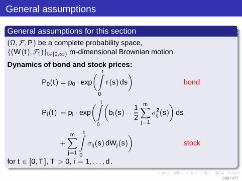
General assumptions
General assumptions for this section(Ω,F , P) be a complete probability space,(W (t),Ft )t∈[0,∞) m-dimensional Brownian motion.
Dynamics of bond and stock prices:
P0(t) = p0 · exp( t∫
0
r(s) ds)
bond
Pi(t) = pi · exp( t∫
0
(bi(s) − 1
2
m∑
j=1
σ2ij (s)
)ds
+
m∑
j=1
t∫
0
σij(s) dWj(s)
)stock
for t ∈ [0, T ], T > 0, i = 1, . . . , d .
399 / 477
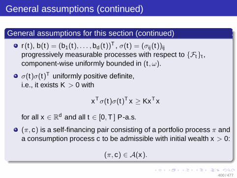
General assumptions (continued)
General assumptions for this section (continued)
r(t), b(t) = (b1(t), . . . , bd (t))T , σ(t) = (σij(t))ij
progressively measurable processes with respect to Ftt ,component-wise uniformly bounded in (t , ω).
σ(t)σ(t)T uniformly positive definite,i.e., it exists K > 0 with
xT σ(t)σ(t)T x ≥ KxT x
for all x ∈ Rd and all t ∈ [0, T ] P-a.s.
(π, c) is a self-financing pair consisting of a portfolio process π anda consumption process c to be admissible with initial wealth x > 0:
(π, c) ∈ A(x).
400 / 477

Solution approaches (continuous-time market model)
Two approaches:
Stochastic control approach (Robert/Merton)
Martingale method (Cox/Huang, Karatzas/Lehoczky/Shreve,Pliska)
401 / 477

Formulation of the problem
Introduce a functional J which measures the utility of a paymentstream (large value = good payment stream).
For a given initial wealth x > 0 an investor looks for aself-financing pair (π, c) ∈ A(x) which maximizes the expectedutility from consumption and / or terminal wealth
J(x ;π, c) = E( T∫
0
U1(t , c(t)
)dt + U2
(X (T )
))
Notation:
X (t) wealth corresponding to x and (π, c).U1, U2 utility functions.
402 / 477

Utility functions
Definition(1) Let U : (0,∞) → R be a strictly concave and continuously
differentiable function with
U ′(0) := limx↓0
U ′(x) = +∞, U ′(∞) := limx→∞
U ′(x) = 0.
Then U is called a utility function.
(2) A continuous function U : [0, T ] × (0,∞) → R such that for allt ∈ [0, T ] the function U(t , ·) is a utility function in the sense of (1)is called a utility function.
403 / 477

Examples of utility functions
Examples :
(1) U(x) = ln(x)
(2) U(x) =√
x
(3) U(x) = xα for 0 < α < 1
(4) U(t , x) = e−ρt · U1(x), ρ > 0 with U1 as in (1) or (2).
404 / 477

Utility functions
RemarkA utility function is strictly increasing
⇒ each additional wealth leads to additional utility.
A utility function is strictly concave
⇒ U ′(x) is strictly decreasing
⇒ decreasing marginal utility
⇒ the gain of utility from one additional unit of moneydecreases with increasing x .
405 / 477

Utility functions
Remark (continued)The marginal utility in x = 0 is infinite"a tiny bit is much more than nothing"
Vanishing marginal utility in x = ∞ models a saturation effect.
A wider class of utility functions can be considered. In particularthe (popular but criticized) quadratic utility function
U(x) = −12(x − a)2.
406 / 477

Formulation of the problem
RemarkFor an arbitrary (π, c) ∈ A(x) the expectation in J(x ;π, c) is notnecessarily defined.
We can restrict the class of self-financing pairs (π, c) to all thosefor which the expectation in (π, c) ∈ A(x) is finite.
We require only a weak integrability condition for a feasible pair(π, c).
407 / 477

Continuous-time portfolio problem
Continuous-time portfolio problem
max(π,c)∈A′(x)
J(x ;π, c)
with
A′(x) =
(π, c) ∈ A(x)
∣∣∣∣E( T∫
0
U1(t , c(t)
)− dt + U2(X (T )
)−)
< ∞
408 / 477

Continuous-time portfolio problem
Remark(1) By restricting to the set A′(x), the integral in J is defined.
The expectation exists but can be equal to infinity.
(2) In the case of positive utility functions, U1(t , ·) > 0 andU2(t , ·) > 0, the equality A(x) = A′(x) is satisfied.
409 / 477

Outline
5 Optimal PortfoliosIntroduction and Formulation of the ProblemThe martingale methodOptimal Option PortfoliosExcursion 8: Stochastic ControlMaximize expected value in presence of quadratic control costsIntroductionPortfolio Optimization via Stochastic Control Method
410 / 477

General assumption / notation→ completeness of the market
General assumption for this section
d = m
Notation
γ(t) := exp(−
t∫
0
r(s) ds)
θ(t) := σ−1(t)(b(t) − r(t) 1
)
Z (t) := exp(−
t∫
0
θ(s)T dW (s) − 12
t∫
0
‖θ(s)‖2 ds)
H(t) := γ(t) · Z (t)
411 / 477

The main idea
The martingale method is based on a separation of the dynamicalproblem into
a static optimization problem(determination of the optimal payoff profile)
a representation problem(compute the portfolio process correspondingto the optimal payoff profile).
412 / 477
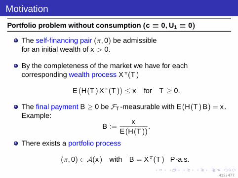
Motivation
Portfolio problem without consumption (c ≡ 0, U1 ≡ 0)
The self-financing pair (π, 0) be admissiblefor an initial wealth of x > 0.
By the completeness of the market we have for eachcorresponding wealth process Xπ(T )
E(H(T ) Xπ(T )
)≤ x for T ≥ 0.
The final payment B ≥ 0 be FT -measurable with E(H(T ) B) = x .Example:
B :=x
E(H(T )).
There exists a portfolio process
(π, 0) ∈ A(x) with B = Xπ(T ) P-a.s.
413 / 477
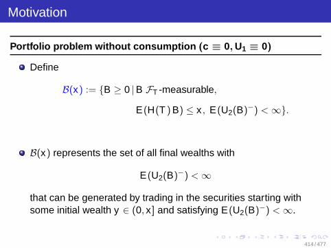
Motivation
Portfolio problem without consumption (c ≡ 0, U1 ≡ 0)
Define
B(x) := B ≥ 0 |B FT -measurable,
E(H(T ) B) ≤ x , E(U2(B)−) < ∞.
B(x) represents the set of all final wealths with
E(U2(B)−) < ∞
that can be generated by trading in the securities starting withsome initial wealth y ∈ (0, x ] and satisfying E(U2(B)−) < ∞.
414 / 477
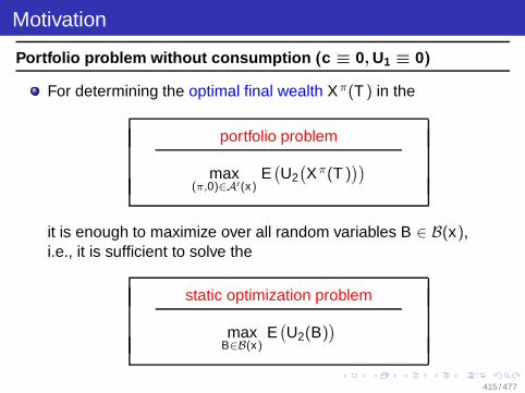
Motivation
Portfolio problem without consumption (c ≡ 0, U1 ≡ 0)
For determining the optimal final wealth Xπ(T ) in the
portfolio problem
max(π,0)∈A′(x)
E(U2(Xπ(T )
))
it is enough to maximize over all random variables B ∈ B(x),i.e., it is sufficient to solve the
static optimization problem
maxB∈B(x)
E(U2(B)
)
415 / 477

Motivation
Portfolio problem without consumption (c ≡ 0, U1 ≡ 0)
If B∗ is an optimal final wealth in the static optimization problem,then to solve the portfolio problem we have to solve the
representation problem
Find a (π, 0) ∈ A′(x)
with Xπ(T ) = B∗ P-a.s.
416 / 477
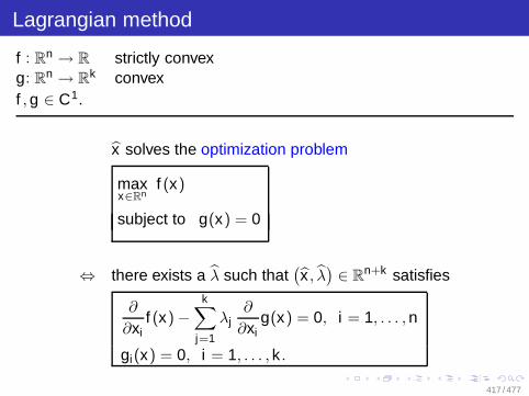
Lagrangian method
f : Rn → R strictly convex
g: Rn → R
k convexf , g ∈ C1.
x solves the optimization problem
maxx∈Rn
f (x)
subject to g(x) = 0
⇔ there exists a λ such that(x , λ
)∈ R
n+k satisfies
∂
∂xif (x) −
k∑
j=1
λj∂
∂xig(x) = 0, i = 1, . . . , n
gi(x) = 0, i = 1, . . . , k .
417 / 477

Lagrangian method
In words:(x , λ
)∈ R
n+k is a zero of the derivative of the
Lagrangian function
L(x , λ) = f (x) − λT g(x)
418 / 477

The Lagrangian method for the portfolio problem
Consider the static optimization problem
maxB∈B(x)
E(U2(B)
).
Lagrangian function
L(B, y) := E(U2(B) − y ·
(H(T ) B − x
)), y > 0.
Formally differentiating L with respect to B and yand interchanging the expectation withthe differentiating process yields
0 = LB(B, y) = E(U ′
2(B) − y H(T )),
0 = Ly (B, y) = x − E(H(T ) B
).
419 / 477

The Lagrangian method for the portfolio problem
A random variable B satisfying
U ′2(B) − y H(T ) = 0 P-a.s.
solves the first equation.
The range of U ′2(.) equals R
+ and U ′2(.) is strictly decreasing.
Therefore, it can be inverted on R+ and we obtain
B =(U ′
2
)−1(y · H(T )).
Putting this in the second equation yields
0 = x − E(H(T ) ·
(U ′
2
)−1(y · H(T ))
)︸ ︷︷ ︸
=:χ(y)
.
If we can solve this equation uniquely for y then we have found acandidate for the optimal final wealth.
420 / 477

The Lagrangian method for the portfolio problem
DefineY (u) := χ−1(u), I2 :=
(U ′
2
)−1.
Candidate for the optimal final wealth
B∗ = I2(Y (x) · H(T )
)> 0.
Prove that B∗ is the optimal final wealth.
421 / 477

Notation
Notation
I2(y) :=(U ′
2
)−1(y) for y ∈ (0,∞)
I1(t , y) :=(U ′
1
)−1(t , y) for y ∈ (0,∞)
χ(y) := E( T∫
0
H(t) I1(t , y ·H(t)
)dt + H(T ) I2
(y · H(T )
))
422 / 477
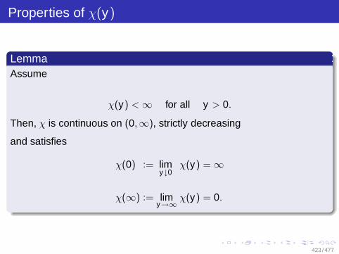
Properties of χ(y)
LemmaAssume
χ(y) < ∞ for all y > 0.
Then, χ is continuous on (0,∞), strictly decreasing
and satisfies
χ(0) := limy↓0
χ(y) = ∞
χ(∞) := limy→∞
χ(y) = 0.
423 / 477
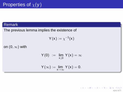
Properties of χ(y)
RemarkThe previous lemma implies the existence of
Y (x) := χ−1(x)
on (0,∞) with
Y (0) := limx↓0
Y (x) = ∞
Y (∞) := limx→∞
Y (x) = 0.
424 / 477

Utility functions
Lemma
Let U be a utility function with I :=(U ′)−1. Then we have
U(I(y)
)≥ U(x) + y(I(y) − x)
for 0 < y, x < ∞.
425 / 477

Optimal consumption / optimal terminal wealth
Theorem: Optimal consumption and optimal terminal wealthConsider the portfolio problem. Let x > 0 and χ(y) < ∞ for all y > 0.Set
Y (x) := χ−1(x).
Then, for
B∗ := I2(Y (x) · H(T )
)optimal terminal wealth
c∗(t) := I1(t , Y (x) · H(T )
)optimal consumption
there exists a self-financing portfolio process π∗(t), t ∈ [0, T ], such that(π∗, c∗) ∈ A′(x), X x,π∗,c∗
(T ) = B∗ P-a.s.
and such that(π∗, c∗) solves the portfolio problem. Here, X x,π∗,c∗
(t) isthe wealth process corresponding to the pair
(π∗, c∗) and the initial
wealth x .
426 / 477
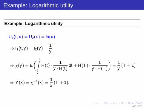
Example: Logarithmic utility
Example: Logarithmic utility
U1(t , x) = U2(x) = ln(x)
⇒ I1(t , y) = I2(y) =1y
⇒ χ(y) = E( T∫
0
H(t) · 1y · H(t)
dt + H(T ) · 1y · H(T )
)=
1y
(T + 1)
⇒ Y (x) = χ−1(x) =1x
(T + 1).
427 / 477

Example: Logarithmic utility
Optimal consumption
c∗(t) = I1(t , Y (x) · H(t)
)=
xT + 1
· 1H(t)
Optimal final wealth
B∗ = I2(Y (x) · H(t)
)=
xT + 1
· 1H(T )
428 / 477
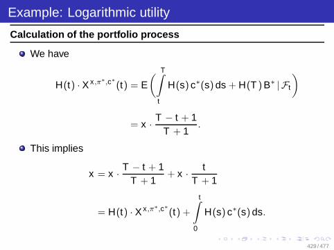
Example: Logarithmic utility
Calculation of the portfolio process
We have
H(t) · X x,π∗,c∗
(t) = E( T∫
t
H(s) c∗(s) ds + H(T ) B∗ | Ft
)
= x · T − t + 1T + 1
.
This implies
x = x · T − t + 1T + 1
+ x · tT + 1
= H(t) · X x,π∗,c∗
(t) +
t∫
0
H(s) c∗(s) ds.
429 / 477

Example: Logarithmic utility
Calculation of the portfolio process
Application of Ito’s formula to the product H(t) · X x,π∗,c∗(t) yields
x = x +
t∫
0
H(s) · X x,π∗,c∗
(s)(π∗(s)T σ(s) − θ(s)T )
︸ ︷︷ ︸=: f (s)
dW (s).
Hence we must have
f (s) = 0 P-a.s. for all s ∈ [0, T ].
As H(s) · X x,π∗,c∗(s) is positive we thus obtain
π∗(t) =(σ(t)T )−1
θ(t) for all t ∈ [0, T ].
In the special case of d = 1 and constant coefficients r , b, σ we get
π∗(t) =b − rσ2 local risk for stock investment
430 / 477
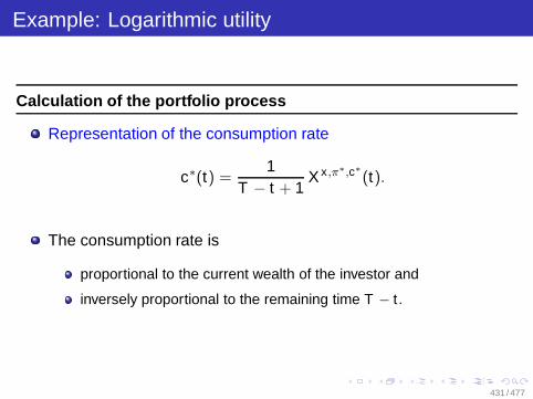
Example: Logarithmic utility
Calculation of the portfolio process
Representation of the consumption rate
c∗(t) =1
T − t + 1X x,π∗,c∗
(t).
The consumption rate is
proportional to the current wealth of the investor and
inversely proportional to the remaining time T − t .
431 / 477

Solution of the representation problem
Theorem: Solution of the representation problemConsider the portfolio problem.Let x > 0 and assume χ(y) < ∞ for all y > 0. Let
B∗ := I2(Y (x) · H(T )
), c∗(t) := I1
(t , Y (x) · H(T )
).
If there exists a function f ∈ C1,2([0, T ] × R
d)
with f (0, 0, . . . , 0) = xand
1H(T )
· E( T∫
t
H(s) c∗(s) ds + H(T ) B∗ | Ft
)= f(t , W1(t), . . . , Wd (t)
),
then for all t ∈ [0, t] we have
π∗(t) =1
X x,π∗,c∗(t)σ−1(t)∇x f
(t , W1(t), . . . , Wd (t)
).
432 / 477

Optimal consumption / optimal terminal wealth
Corollary(1) The optimal terminal wealth B∗ of the problem
max(π,0)∈A′(x)
E(U2(X x,π(T )
))
is given by
B∗ := I2(Y (x) · H(T )
)
where in the definition of χ(y) we have to set I1(t , y) ≡ 0.
433 / 477
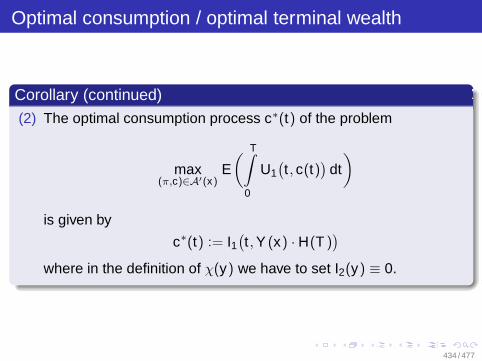
Optimal consumption / optimal terminal wealth
Corollary (continued)
(2) The optimal consumption process c∗(t) of the problem
max(π,c)∈A′(x)
E( T∫
0
U1(t , c(t)
)dt)
is given by
c∗(t) := I1(t , Y (x) · H(T )
)
where in the definition of χ(y) we have to set I2(y) ≡ 0.
434 / 477

Outline
5 Optimal PortfoliosIntroduction and Formulation of the ProblemThe martingale methodOptimal Option PortfoliosExcursion 8: Stochastic ControlMaximize expected value in presence of quadratic control costsIntroductionPortfolio Optimization via Stochastic Control Method
435 / 477

General assumption / notation
General assumption for this section
d = m
Notation
γ(t) := exp(−
t∫
0
r(s) ds)
θ(t) := σ−1(t)(b(t) − r(t) 1
)
Z (t) := exp(−
t∫
0
θ(s)T dW (s) − 12
t∫
0
‖θ(s)‖2 ds)
H(t) := γ(t) · Z (t)
436 / 477

Description of the market model
RestrictionThe market coefficients r , b, σ are constant.
437 / 477

Description of the market model
Consider
a market, where a bond, d stocks, and d options on these stocksare traded
a Portfolio consisting of the bond and the options.
Assume
The options have a price process of the form
f (i)(t , P1(t), . . . , Pd (t)), i = 1, . . . , d , f ∈ C1,2
Option prices satisfy certain requirements(particularly satisfied for European puts and calls in theBlack-Scholes model).
438 / 477

Description of the market model
Admissible trading strategy in bond and options:
ϕ(t) =(ϕ0(t), ϕ1(t), . . . , ϕd (t)
)
The integralst∫
0
ϕ0(s) dP0(s)
t∫
0
ϕi(s) df (i)(s, P1(s), . . . , Pd (s))
are assumed to be defined.ϕ(t) is assumed to be Ft -progressively measurable.Wealth progress
X (t) = ϕ0(t) P0(t) +
d∑
i=1
ϕi(t) f (i)(t , P1(t), . . . , Pd (t)).
439 / 477

The problem
Consider the problem
maxϕ
E(U(X (T ))
)
where U is a utility function.
440 / 477

Motivation of the solution of the problem
To motivate the solution of the problem, we take a look at the followingdiagrams representing
the solution of the option pricing problemvia the replication approach and
the solution of the portfolio problemvia the martingale approach.
The third diagram will show the solution of the problem.
441 / 477

Option pricing
option priceEQ(e−rT B
) terminal payoffB
?oo
=
cost of replication
X ∗(0)
=
OO
replication strategyXπ∗
(T )
π∗(t)oo
Starting out from the final payment B of an option we replicate the finalpayment via following a suitable portfolio strategy leading to a finalwealth that coincides with final option payment. Then, the costs ofsetting up the cheapest replication strategy yield the option price.
442 / 477

Portfolio optimization with stocks
initial wealthx
? // optimal terminal wealthX x,π∗
(T )
optimal final paymentB∗
// replication strategyπ∗(t)
OO
The given inital wealth x will be invested according to a portfolioprocess π∗(t) with the aim to obtain a terminal wealth which promisesthe highest possible utility (we ignore the possibility of consumption).To do so, we first determine an optimal final payoff B∗ and then look fora replication strategy for B∗.
443 / 477
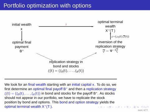
Portfolio optimization with options
initial wealthx
? //optimal terminal
wealthX ∗(T )
optimal finalpayment
B∗
((QQQQQQQQQQQ
inversion of thereplication strategy
ϕ = Ψ−1ξ
ϕ=(ϕ0(t),ϕ(t))
OO
replication strategy inbond and stocks
ξ(t) = (ξ0(t), . . . , ξd (t))
66mmmmmmmmmm
We look for an final wealth starting with an initial capital x . To do so, wefirst determine an optimal final payoff B∗ and then a replication strategyξ(t) = (ξ0(t), . . . , ξd (t)) in bond and stocks for the payoff B∗. As stocksshould not appear in our portfolio, we have to replicate the stockposition by bond and options. This bond and option strategy yields theoptimal terminal wealth X ∗(T ).
444 / 477

Motivation of the solution of the problem
TheoremLet the Delta matrix
Ψ(t) =(Ψij(t)
)ij , i , j = 1, . . . , d
withΨij := f (i)
pj
(t , P1(t), . . . , Pd (t)
)
be regular for all t ∈ [0, T ]. Then, the option portfolio problempossesses the following explicit solution:
(1) The optimal terminal wealth B∗ coincides with the optimal terminalwealth of the corresponding stock portfolio problem.
445 / 477
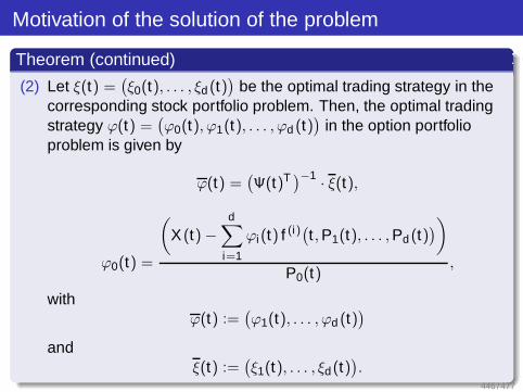
Motivation of the solution of the problem
Theorem (continued)
(2) Let ξ(t) =(ξ0(t), . . . , ξd (t)
)be the optimal trading strategy in the
corresponding stock portfolio problem. Then, the optimal tradingstrategy ϕ(t) =
(ϕ0(t), ϕ1(t), . . . , ϕd (t)
)in the option portfolio
problem is given by
ϕ(t) =(Ψ(t)T )−1 · ξ(t),
ϕ0(t) =
(X (t) −
d∑
i=1
ϕi(t) f (i)(t , P1(t), . . . , Pd (t)))
P0(t),
withϕ(t) :=
(ϕ1(t), . . . , ϕd (t)
)
andξ(t) :=
(ξ1(t), . . . , ξd(t)
).
446 / 477
Motivation of the solution of the problem
Remark(1) Under the given assumptions, the optimal final wealth only
depends on the utility functions but not on the choice of thetradable securities.
(2) The optimal trading strategy depends on the traded options viathe delta matrix (more precisely: via the replication strategy for theoptions).
447 / 477
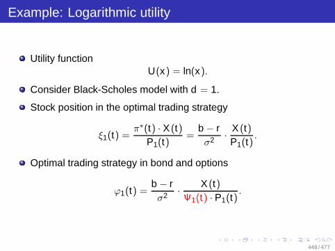
Example: Logarithmic utility
Utility functionU(x) = ln(x).
Consider Black-Scholes model with d = 1.
Stock position in the optimal trading strategy
ξ1(t) =π∗(t) · X (t)
P1(t)=
b − rσ2 · X (t)
P1(t).
Optimal trading strategy in bond and options
ϕ1(t) =b − rσ2 · X (t)
Ψ1(t) · P1(t).
448 / 477
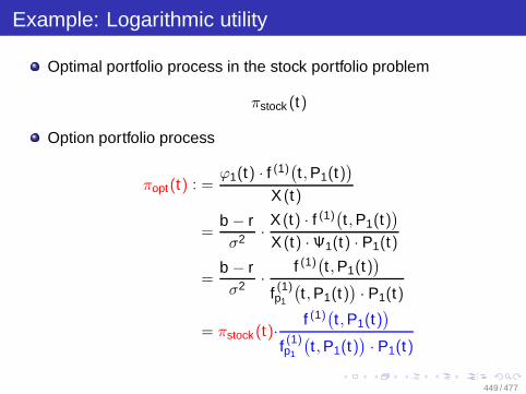
Example: Logarithmic utility
Optimal portfolio process in the stock portfolio problem
πstock (t)
Option portfolio process
πopt(t) : =ϕ1(t) · f (1)
(t , P1(t)
)
X (t)
=b − rσ2 · X (t) · f (1)
(t , P1(t)
)
X (t) · Ψ1(t) · P1(t)
=b − rσ2 · f (1)
(t , P1(t)
)
f (1)p1
(t , P1(t)
)· P1(t)
= πstock (t)· f (1)(t , P1(t)
)
f (1)p1
(t , P1(t)
)· P1(t)
449 / 477

Example: Logarithmic utility
TheoremWith the choice of
U(x) = ln(x),
in the Black-Scholes model with d = 1 we have
(1) πopt(t) = πstock (t) for all t ∈ [0, T ]
⇔ f (1)(t , P1(t)
)= k · P1(t) for a constant k ∈ R \ 0.
(2) In the case of a European call option we have
πopt(t) < πstock (t)
for all t ∈ [0, T ].
450 / 477
Example: Logarithmic utility
Remark(1) states that in the Black-Scholes model, πopt(t) is constant ifand only if the payoff of the contingent claims is a multiple of theunderlying stock price.
(2) says that with the choice of a European call option, in theoption portfolio problem the optimal capital which is invested in therisky asset is always smaller than the corresponding risky positionin the stock portfolio problem.
451 / 477
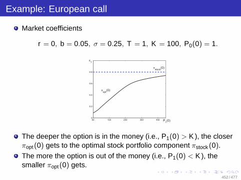
Example: European call
Market coefficients
r = 0, b = 0.05, σ = 0.25, T = 1, K = 100, P0(0) = 1.
50 150 250 350 4500
0.2
0.4
0.6
0.8
p1
P1(0)
pstock
(0)
popt
(0)
The deeper the option is in the money (i.e., P1(0) > K ), the closerπopt(0) gets to the optimal stock portfolio component πstock (0).
The more the option is out of the money (i.e., P1(0) < K ), thesmaller πopt(0) gets.
452 / 477

Outline
5 Optimal PortfoliosIntroduction and Formulation of the ProblemThe martingale methodOptimal Option PortfoliosExcursion 8: Stochastic ControlMaximize expected value in presence of quadratic control costsIntroductionPortfolio Optimization via Stochastic Control Method
453 / 477

General Assumptions
General assumptions for this section
Let X (t) be an n-dimensional Ito process.
Controlled SDEControlled stochastic differential equation:
dX (t) = µ(t , X (t), u(t)) dt + σ(t , X (t), u(t)) dW (t)
where W (t) is an m-dimensional Brownian motion andu(t) a d -dimensional stochastic process (the control).
454 / 477
Outline
5 Optimal PortfoliosIntroduction and Formulation of the ProblemThe martingale methodOptimal Option PortfoliosExcursion 8: Stochastic ControlMaximize expected value in presence of quadratic control costsIntroductionPortfolio Optimization via Stochastic Control Method
455 / 477
Example
Be X (t) = x + W (t) +t∫
0u(s) ds controlled process with 1-dimensional
Brownian motion W (t), as control action choose intensity u(t) of driftprocess at each time instant t ∈ [0, T ].Consider the problem to minimize (a, b > 0):
E
T∫
0
au2(t) dt − bX (T )
Under suitable requirements on u(t) we get
E(X (T )) = x + E
T∫
0
u(s) ds
and hence
E
T∫
0
(au2(t) − bu(t)) dt − bx
456 / 477
Example
Minimizing function u(t) under the integral leadsto the optimal choice of
u∗(t) =b2a
.
457 / 477

Outline
5 Optimal PortfoliosIntroduction and Formulation of the ProblemThe martingale methodOptimal Option PortfoliosExcursion 8: Stochastic ControlMaximize expected value in presence of quadratic control costsIntroductionPortfolio Optimization via Stochastic Control Method
458 / 477
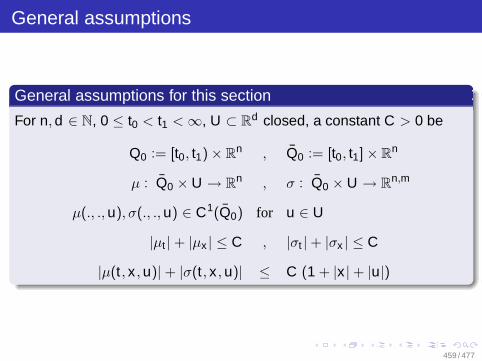
General assumptions
General assumptions for this section
For n, d ∈ N, 0 ≤ t0 < t1 < ∞, U ⊂ Rd closed, a constant C > 0 be
Q0 := [t0, t1) × Rn , Q0 := [t0, t1] × R
n
µ : Q0 × U → Rn , σ : Q0 × U → R
n,m
µ(., ., u), σ(., ., u) ∈ C1(Q0) for u ∈ U
|µt | + |µx | ≤ C , |σt | + |σx | ≤ C
|µ(t , x , u)| + |σ(t , x , u)| ≤ C (1 + |x | + |u|)
459 / 477

Notations
If the process X (t) solves the controlled SDE with an initial value of xat time t , then we indicate this by denoting its expectation at time t by
E t,x(X (s)).
460 / 477

Notations
Define for an open set O ⊂ Rn
Q := [t0, t1) × O,
Q := [t0, t1] × O,
τ := inft ≥ t0 | (t , X (t)) /∈ Q.
Define the cost function
J(t , x , u) = E t,x
τ∫
t
L(s, X (s), u(s)) ds + Ψ(τ, X (τ))
461 / 477

Notations
L,Ψ are continuous functions with
|L(t , x , u)| ≤ C(
1 + |x |k + |u|k)
,
|Ψ(t , x)| ≤ C(
1 + |x |k)
,
for some k ∈ N on Q × U or on Q.
L(s, X (s), u(s)) is called running costs and Ψ(τ, X (τ)) is calledterminal costs.
462 / 477

Notations
V (t , x) := infu∈A(t,x)
J(t , x ; u) (t , x) ∈ Q
is called value function, where A(t , x) denotes the set of all admissiblecontrols u(·).
463 / 477
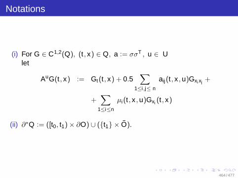
Notations
(i) For G ∈ C1,2(Q), (t , x) ∈ Q, a := σσT , u ∈ Ulet
AuG(t , x) := Gt(t , x) + 0.5∑
1≤i ,j≤ n
aij(t , x , u)Gxi xj +
+∑
1≤i≤n
µi(t , x , u)Gxi (t , x)
(ii) ∂∗Q := ([t0, t1) × ∂O) ∪ (t1 × O).
464 / 477

Contolled SDE
Definition–Part IBe (Ω,F , Ftt∈[t0,t1]
, P) probability space with filtration. A U-valuedprogressively measurable process u(t), t ∈ [t0, t1] is called admissiblecontrol, if for all values x ∈ R
n the SDE with initial condition X (t0) = xpossess a unique solution X (t)t∈[t0 ,t1] and if we have
465 / 477

Contolled SDE
Definition–Part II
E
t1∫
t0
|u(s)|k ds
< ∞,
E t,x(||X (·)| |k
):= E t,x
(sup
s∈[t,t1]|X (s)|k
)< ∞
for all k ∈ N.
466 / 477

Controlled SDE
Theorem–Part I
Be G ∈ C1,2(Q) ∩ C(Q) with |G(t , x)| ≤ K(
1 + |x |k)
for some suitable
constants K > 0, k ∈ N, a solution to the Hamilton-Jacobi-Bellmanequation:
infu∈U
(AuG(t , x) + L(t , x , u)) = 0 (t , x) ∈ Q,
G(t , x) = Ψ(t , x) (t , x) ∈ ∂∗Q.
Then we have
467 / 477
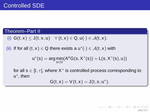
Controlled SDE
Theorem–Part II(i) G(t , x) ≤ J(t , x , u) ∀ (t , x) ∈ Q, u(·) ∈ A(t , x).
(ii) If for all (t , x) ∈ Q there exists a u∗(·) ∈ A(t , x) with
u∗(s) = arg minu∈U
(AuG(s, X ∗(s)) + L(s, X ∗(s), u))
for all s ∈ [t , τ ], where X ∗ is controlled process corresponding tou∗, then
G(t , x) = V (t , x) = J(t , x ; u∗).
468 / 477

Outline
5 Optimal PortfoliosIntroduction and Formulation of the ProblemThe martingale methodOptimal Option PortfoliosExcursion 8: Stochastic ControlMaximize expected value in presence of quadratic control costsIntroductionPortfolio Optimization via Stochastic Control Method
469 / 477
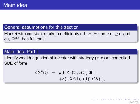
Main idea
General assumptions for this sectionMarket with constant market coefficients r , b, σ. Assume m ≥ d andσ ∈ R
d ,m has full rank.
Main idea–Part IIdentify wealth equation of investor with strategy (π, c) as controlledSDE of form
dX u(t) = µ(t , X u(t), u(t)) dt +
+σ(t , X u(t), u(t)) dW (t),
470 / 477

Main idea
Main idea–Part IIwhere µ, σ, u have special form
u = (u1, u2) := (π, c),
µ(t , x , u) = (r + uT1 (b − r 1))x − u2,
σ(t , x , u) = xuT1 σ.
471 / 477
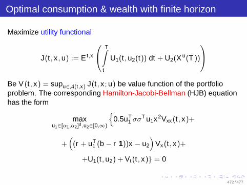
Optimal consumption & wealth with finite horizon
Maximize utility functional
J(t , x , u) := E t,x
T∫
t
U1(t , u2(t)) dt + U2(Xu(T ))
Be V (t , x) = supu∈A(t,x) J(t , x ; u) be value function of the portfolioproblem. The corresponding Hamilton-Jacobi-Bellman (HJB) equationhas the form
maxu1∈[α1,α2]d ,u2∈[0,∞)
0.5uT
1 σσT u1x2Vxx (t , x)+
+((r + uT
1 (b − r 1))x − u2
)Vx (t , x)+
+U1(t , u2) + Vt(t , x) = 0
472 / 477

Optimal consumption & wealth with finite horizon
V (T , x) = U2(x)
for given constants α1, α2 ∈ R, α1 ≤ α2.
Solution of the corresponding HJB equationSolve the HJB equation for the special choice of
U1(t , c) =1γ
e−βtcγ , U2(x) =1γ
xγ
with β > 0 , γ ∈ (0, 1).
473 / 477
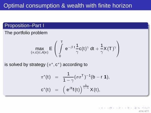
Optimal consumption & wealth with finite horizon
Proposition–Part IThe portfolio problem
max(π,c)∈A(x)
E
T∫
0
e−β t 1γ
c(t)γ dt +1γ
X (T )γ
is solved by strategy (π∗, c∗) according to
π∗(t) =1
1 − γ(σσT )−1(b − r 1),
c∗(t) =(
eβt f (t)) 1
γ−1X (t),
474 / 477

Optimal consumption & wealth with finite horizon
Proposition–Part IIwhere f (t) is given by
a1 := −0.5(b − r 1)T (σσT )−1(b − r 1)1
γ − 1+ r ,
a2 :=1 − γ
γe
βtγ−1 ,
g(t) = ea1
1−γ(T−t) +
+1 − γ
γ(a1 − β)
(e
a1−β
1−γT − e
a1−β
1−γt)
ea1
1−γ(T−t),
g(t) = f (t)γ
1−γ .
475 / 477

For Further Reading
R. Korn and E. KornOption Pricing and Portfolio Optimization -Modern methods of financial mathematics, AMS, 2001.
Gerhard-Wilhelm WeberFurther documents distributed in the course.
476 / 477