Embed Size (px)
Citation preview

Faculty of Sciences
Geostatistical analysis of the regeneration of
Sycamore (Acer pseudoplatanus) in Flanders
(Belgium)
by
ir. Thierry Onkelinx
Promoters:
Prof. Dr. ir. M. Van Meirvenne, Department of Soil Management
Prof. Dr. ir. K. Verheyen, Department of Forest and Water Management
Dr. D. Bauwens, Research Institute for Nature and Forest
Master dissertation submitted to obtain the degree of
Master of Statistical Data Analysis
Academic year 2008–2009


iii
Preface
This thesis is the final piece of my education as a master in statistical data analysis.
The master course revealed to me how fascinating the world of statistics can be. The
thesis allowed me to explore three of my favourite research topics: forestry, geographical
information science and statistics.
First of all I would like to express my gratitude to ir. Paul Quataert of the Research
Institute for Nature and Forest (INBO). He gave me the necessary facilities to combine
my full-time job with the master course during 4 years. Furthermore he encourages our
team to keep up-to-date with the current evolutions in statistics.
This thesis was not feasible without the dendrometrical data. Therefore my thanks go
out to dr. ir. Martine Waterinckx, Bart Roelandt and ir. Wout Damiaans (all Nature and
Forestry Agency, ANB) for kindly providing the data of the national forest inventory and
the forest management plans. ir. Kris Vandekerkhove, ir. Luc De Keersmaeker and Peter
Van de Kerkhove (all INBO) kindly providing the data of the forest reserves. All this data
are confidential to the extent that we can only distribute the results of our study but not
the data itself.
I could not have finalised this thesis without the input of my promoters: prof. dr. ir.
Marc Van Meirvenne (UGent), prof. dr. ir. Kris Verheyen (UGent) and dr. Dirk Bauwens
(INBO). They were willing to guide me through my thesis based on my first rough ideas
on the topic. Their invaluable comments helped me to clearly define the scope of this
thesis. Special thanks go to dr. Dirk Bauwens for expertly proof-reading this thesis.
And last but not least I own many thanks to Ester, my future wife. She took care of
many things so I could spend enough time on my thesis and the courses.
ir. Thierry Onkelinx, june 2009


v
Admission for circulating the work
The author and the promoters give permission to consult this master dissertation and to
copy it or parts of it for personal use. Each other use falls under the restrictions of the
copyright, in particular concerning the obligation to mention explicitly the source when
using results of this master dissertation.
ir. Thierry Onkelinx, june 2009

vi

CONTENTS vii
Contents
Preface ii
Table of contents v
1 Abstract 1
2 Introduction 3
2.1 Goals . . . . . . . . . . . . . . . . . . . . . . . . . . . . . . . . . . . . . . . 3
2.2 The data sets . . . . . . . . . . . . . . . . . . . . . . . . . . . . . . . . . . 3
2.2.1 Sampling technique . . . . . . . . . . . . . . . . . . . . . . . . . . . 4
2.2.2 Measure for success of regeneration . . . . . . . . . . . . . . . . . . 5
3 Modelling and predicting ecological data 7
3.1 Analysing spatially auto-correlated data . . . . . . . . . . . . . . . . . . . 7
3.1.1 Auto-covariate models . . . . . . . . . . . . . . . . . . . . . . . . . 7
3.1.2 Generalised least squares regression . . . . . . . . . . . . . . . . . . 8
3.1.3 Autoregressive models . . . . . . . . . . . . . . . . . . . . . . . . . 8
3.1.4 Spatial generalised linear mixed models (GLMM) . . . . . . . . . . 9
3.1.5 Spatial generalised estimating equations (GEE) . . . . . . . . . . . 9
3.2 Regression models for count data . . . . . . . . . . . . . . . . . . . . . . . 10
3.3 Assessing the impact of capturing spatial auto-correlation . . . . . . . . . . 10
3.3.1 Selected methods . . . . . . . . . . . . . . . . . . . . . . . . . . . . 10
3.3.2 Comparing model parameters . . . . . . . . . . . . . . . . . . . . . 13
3.3.3 Assessing the quality of the predictions . . . . . . . . . . . . . . . . 14
3.4 Parametric spatial bootstrap . . . . . . . . . . . . . . . . . . . . . . . . . . 15
4 Material and methods 17
4.1 Creating a data set . . . . . . . . . . . . . . . . . . . . . . . . . . . . . . . 17
4.2 Building the models . . . . . . . . . . . . . . . . . . . . . . . . . . . . . . . 17
4.2.1 Tested variables . . . . . . . . . . . . . . . . . . . . . . . . . . . . . 17
4.2.2 Model selection . . . . . . . . . . . . . . . . . . . . . . . . . . . . . 18
4.3 Bootstrapping the model parameters . . . . . . . . . . . . . . . . . . . . . 21
4.4 Cross-validation . . . . . . . . . . . . . . . . . . . . . . . . . . . . . . . . . 22
4.4.1 Basics . . . . . . . . . . . . . . . . . . . . . . . . . . . . . . . . . . 22
4.4.2 Working around some problems . . . . . . . . . . . . . . . . . . . . 23

viii CONTENTS
5 Results 25
5.1 Influence on model parameters . . . . . . . . . . . . . . . . . . . . . . . . . 25
5.1.1 Models assuming Gaussian data . . . . . . . . . . . . . . . . . . . . 25
5.1.2 Models assuming Poisson data . . . . . . . . . . . . . . . . . . . . . 33
5.1.3 Models assuming binomial data . . . . . . . . . . . . . . . . . . . . 39
5.2 Influence on cross-validation of predictions . . . . . . . . . . . . . . . . . . 44
5.2.1 Models assuming Gaussian data . . . . . . . . . . . . . . . . . . . . 44
5.2.2 Models assuming count data . . . . . . . . . . . . . . . . . . . . . . 47
5.2.3 Models assuming binomial data . . . . . . . . . . . . . . . . . . . . 49
6 Discussion and conclusions 53
6.1 Implications on modeling ecological data . . . . . . . . . . . . . . . . . . . 54
6.2 Summary . . . . . . . . . . . . . . . . . . . . . . . . . . . . . . . . . . . . 55
Bibliography 57
A Exploratory data analysis 63
A.1 Natural regeneration of sycamore . . . . . . . . . . . . . . . . . . . . . . . 63
A.2 Regions . . . . . . . . . . . . . . . . . . . . . . . . . . . . . . . . . . . . . 66
A.3 Geomorphology . . . . . . . . . . . . . . . . . . . . . . . . . . . . . . . . . 67
A.4 Forest management . . . . . . . . . . . . . . . . . . . . . . . . . . . . . . . 69
A.5 Soil . . . . . . . . . . . . . . . . . . . . . . . . . . . . . . . . . . . . . . . . 76
B Overview of the models 79
B.1 Gaussian models . . . . . . . . . . . . . . . . . . . . . . . . . . . . . . . . 79
B.2 Poisson models . . . . . . . . . . . . . . . . . . . . . . . . . . . . . . . . . 84
B.3 Logistic models . . . . . . . . . . . . . . . . . . . . . . . . . . . . . . . . . 87
C Glossary and abbreviations 89
C.1 Glossary . . . . . . . . . . . . . . . . . . . . . . . . . . . . . . . . . . . . . 89
C.2 Abbreviations . . . . . . . . . . . . . . . . . . . . . . . . . . . . . . . . . . 89
C.3 R packages . . . . . . . . . . . . . . . . . . . . . . . . . . . . . . . . . . . . 90

1
Chapter 1
Abstract
Autocorrelation is a very general statistical property of ecological variables observed across
geographic space (Legendre, 1993). Spatial autocorrelation implies that measurements at
locations close to each other exhibit more similar values than those taken at sites that are
further apart (Dormann et al., 2007). Spatial autocorrelation, which comes either from
the physical forcing of environmental variables or from community processes, presents
a problem for statistical testing. Indeed, autocorrelated data violate the assumption of
independence that is made by most standard statistical procedures (Legendre, 1993). The
violation of independent and identically distributed (i.i.d.) residuals may bias parameter
estimates and can increase type I error rates (Bini et al., 2009; Dormann et al., 2007).
Nevertheless, a lot authors still use the basic statistical models and tests that assume i.i.d.
residuals.
We here investigate the impact on both parameter estimates and the model predictions
of incorporating the spatial structure of the data in the statistical model. Therefore we
compare a basic method (assuming i.i.d. residuals) with four methods that deal with the
spatial structure in the data: auto-covariates (AC), generalised least squares (GLS), a
simultaneous autoregressive model (SAR) and a conditional autoregressive model (CAR).
Our case study is a fairly large data set of sycamore (Acer pseudoplatanus) regen-
eration from Flanders (northern part of Belgium). We model the presence-absence data
(binomial), the number of saplings (Poisson) and the log transformed number of saplings
(Gaussian). The explanatory variables are derived from the dendrometrical data or from
available GIS layers.
A spatial parametric bootstrap procedure is used to quantify the distribution of the
model parameter estimates. They show both bias and differences in variance. Mainly the
parameter estimates of explanatory variables with a spatial link are biased and become
more variable. The other explanatory variables exhibit seldom bias. The effect on the
variance depends on the method. Adding auto-covariates has little effect on the variances.
Whereas GLS and SAR results in model parameters with smaller variances for the non-
spatial explanatory variables. CAR results in extremely unstable model parameters.
The predictions are evaluated with a repeated ten-fold cross-validation procedure.

2 1 Abstract
The only differences for the prediction errors is an increased variance for GLS and AC
with Gaussian data. However these variances, remained low. The mean error shows no
significant differences among the methods. Only the AC method for Gaussian and Poisson
data have a significantly higher root mean square error.
We conclude that incorporating the spatial structure of the data into the model clearly
affects the estimates of model parameters for the explanatory variables that have some link
with the spatial structure. The goal of most ecological studies is to interpret the correlation
between the explanatory variables and the response variable. Hence it is important to take
the spatial autocorrelation into account.

3
Chapter 2
Introduction
A good management policy in forestry is to choose tree species with habitat requirements
that match the site conditions. So habitat requirement is an important topic in forestry
research. The nature of forests makes is seldom possible to perform lab experiments. Hence
we need to rely on in situ data. Since the site conditions tend to change gradually, we can
expect that the presence/absence or density of a species will exhibit spatial autocorrela-
tion. In practice authors do not always take this spatial autocorrelation into account, e.g.
Verheyen et al. (2007).
2.1 Goals
In this master thesis we will asses the impact of the spatial autocorrelation by comparing
models with and without a correlation component. We examine the impact on the model
parameters and interpolated maps. The abundance of sycamore (Acer pseudoplatanus) will
serve as a case study. Flanders (Belgium) is at the border of the geographical distribution
of sycamore. And although seldom planted, it turns up at more and more sites. Therefore
we assume that sycamore is mainly spreading by natural regeneration. Hence it will only
appear on locations where the habitat requirement match the site conditions.
2.2 The data sets
The raw data was based on three monitoring schemes: the national (Flemish) forest in-
ventory (NFI), the management plans (MP) and the monitoring in the forest reserves (FR).
All schemes use the same sampling technique with a sample plot area of about 0.1ha. But
each scheme has it own spatial resolution.
The NFI is managed by the Nature and Forestry Agency (ANB). It consists of a 1000m×500m grid across Flanders. This yields a sampling density of 1/50ha−1. All grid points
that coincide with forest are sampled. The results is a somewhat coarse dataset of ca 2500
points that covers the entire territory. All data are collected between 1997 and 1999.

4 2 Introduction
The MP is also managed by ANB. It aggregates the information from the management
plans of forest managed by ANB, which is about 30% of the forested area of Flanders. At
least one point is sampled in each stand. In larger stands more points are sampled in order
to get a sampling density of 1/4ha−1 to 1/2ha−1. The result is a medium scaled network
of about 6000 sampling points divided over 60 forests. All data are collected between 1999
and 2007, but most of it dates from 2002–2004.
The FR is managed by the Research Institute for Nature and Forest (INBO). The
forest reserves are designated areas with a high value for nature conservation. The plots
are located on a 70m× 70m grid. This yields a sampling density of 2ha−1.
2.2.1 Sampling technique
Each plot consists of four concentric circles and one square (fig. 2.1). The first circle
(A1) has a radius of 2.25m. Here the number of seedlings of each species are counted.
Seedlings are smaller than 2 m high. The second circle (A2) has a radius of 4.5m. Here
are the diameter at breast height (dbh, ca 1.50m above ground) of all saplings is measured.
Saplings are taller than 2m high but have a dbh smaller than 7cm. In the third circle (A3),
with 9m radius, all the young trees (7cm ≤ dbh < 39cm) are positioned and their dbh is
measured. The old trees (dbh ≥ 39cm) are positioned and their dbh is measured in the
fourth circle (A4) with a radius of 18m. The 16m× 16m square (V) has the same center
as the concentric circles. In this square a releve of the vegetation is made.
Figure 2.1: Sampling technique with nested plots.

2.2 The data sets 5
2.2.2 Measure for success of regeneration
We use the density (ha−1) of sycamore saplings as a measure for the suitability of the
site conditions for natural regeneration. Saplings are preferred above seedlings because
seedlings only indicate that sycamore can germinate at that site. So the presence of
seedlings does not guaranty a successful regeneration. Saplings indicate that sycamore
could germinate and grow for at least a few years, which implies more chance on a suc-
cessful regeneration. Another benefit is that saplings are measured in plot (A2) with four
times the area of the plot of the seedlings (A1). Since the presence of regeneration can be
rather patchy, we will have a better density estimate for the saplings.

6 2 Introduction

7
Chapter 3
Modelling and predicting ecological
data
3.1 Analysing spatially auto-correlated data
A lot of data in ecology research is collected in the field. We know that nearby sample
sites tend to yield similar measurements. More distant sites are less likely to yield similar
results. The phenomenon is called spatial auto-correlation. As a result the residuals of
a model will no longer be independent and identically distributed (i.i.d.). Hence most
ecological data violate one of the key assumptions of standard statistical data analysis.
This may bias parameter estimates and can increase the type I error rates (falsely rejecting
the null hypothesis).
Dormann et al. (2007) give an overview of methods to account for spatial auto-
correlation. In this chapter we give a short overview of methods that are appropriate
for our analysis.
3.1.1 Auto-covariate models
Auto-covariate models are classical models extended with one or more auto-covariates.
Each auto-covariate is a weighted average of the response at neighbouring locations.
Weight function can depend on geographical or ecological distance between locations.
auto-covariates can be added to normally, binomial and Poisson distributed data. Multi-
ple auto-covariates can be used for anisotropic spatial auto-correlation. Dormann et al.
(2007) found in their simulations that auto-covariate models severely and consistently
underestimated the effects of one of the variables. auto-covariate models can be fit in R
(R Development Core Team, 2009) with the package spdep (Bivand et al., 2009).

8 3 Modelling and predicting ecological data
3.1.2 Generalised least squares regression
In ordinary least squares regression the errors are assumed to be i.i.d. (ε ∼ N(0, σ)).
Generalised least squares regression (GLS) allows to model the spatial auto-correlation
in the error vector by defining a variance-covariance matrix Σ. The error vector is then
ε ∼ N(0,Σ). Some restrictions are placed upon this matrix Σ: a) it must be symmetric
and b) it must be positive definite. This guarantees that the matrix is invertible, which is
necessary for the fitting process.
The values in Σ depend on the inter-point distance through a correlation function.
Typical correlation functions are the exponential, spherical, Gaussian and Matern func-
tion.
The parameters are estimated in two steps. The first step estimates the parameters of
the correlation function by profiling the log-likelihood. The β and σ2 parameters of the
regession model are fixed at their algebraic maximum likelihood estimators. In the second
step the β and σ2 are re-estimated, now conditional on the parameters of the correlation
function from the first step (3.1). The errors are normally distributed after multiplying
all terms with(Σ−1/2
)T(3.2). We could reiterate these steps with the updated estimators
for β and σ. But Hengl (2007) points out that one iteration is often satisfactory. Pinheiro
and Bates (2004) expanded (3.1) to mixed models.
(Σ−1/2
)Ty =
(Σ−1/2
)TXβ +
(Σ−1/2
)Tε (3.1)
(Σ−1/2
)Tε ∼ N(0, σ2I) (3.2)
We have two packages available in R for linear models with GLS: MASS (Venables and
Ripley, 2002) and nlme (Pinheiro et al., 2009). The implementation in both packages is
different. MASS requires the user to fully specify the weight matrix (Σ1/2). Whereas nlme
allows the user to model the correlation through a set of correlation functions. The user
can either fix the parameters of the correlation function or ask the model to fit them too.
3.1.3 Autoregressive models
Autoregressive models come in two flavours: conditional autoregressive models (CAR)
and simultaneous autoregressive models (SAR). Both rely on neighbourhood matrices to
specify the relationship between the response values (CAR) or residuals (SAR) of each
location and it’s neighbouring locations. Hence we require a n×n matrix of spatial weights.
Usually, a binary neighbourhood matrix is formed with nij = 1 when observation j is a
neighbour of observation i. We consider two points to be neighbours if there distance is
within a user defined range. Another option is a matrix with weights depending on the
distance between points through a given function. Closer neighbours get higher weights
than more distant neighbours. Linear autoregressive models can be fit in R with the
package spdep (Bivand et al., 2009).
3.1 Analysing spatially auto-correlated data 9
3.1.4 Spatial generalised linear mixed models (GLMM)
Many common statistical models can be expressed as (generalised) linear models that
incorporate both fixed effects, which are parameters associated with an entire population
or with certain repeatable levels of experimental factors, and random effects, which are
associated with individual experimental units drawn at random from a population. A
model with both fixed effects and random effects is called a mixed-effects model (Pinheiro
and Bates, 2004).
Mixed-effect models are primarily used to describe relationships between a response
variable and some covariates in data that are grouped according to one or more clas-
sification factors. In a spatial context GLMM can be used to incorporate the effects of
(disjunct) regions. By associating common random effects to observations sharing the
same level of a classification factor, mixed-effects models flexibly represent the covariance
structure induced by the grouping of the data.
R has several packages for mixed models, each with their advantages and disadvan-
tages. lme4 (Bates et al., 2009) can cope with crossed or nested random effects in linear,
non-linear, (quasi) binomial and (quasi) Poisson models, but cannot handle correlation
nor variance structures. nlme (Pinheiro et al., 2009) can handle correlation and variance
structures. The drawbacks are that it only handles linear and non-linear models. We can
mimic the logit and log link of binomial and Poisson models, but then we have to assume
that the residuals behave Gaussian instead of binomial or Poisson. Crossed random effects
are not implemented in nlme. MASS (Venables and Ripley, 2002) supplements nlme with a
function for logistic and Poisson models based on the Penalized Quasi-Likelihood (PQL).
According to Bates (2008) the results of PQL (MASS) are less reliable than the Laplace
approximation (lme4).
3.1.5 Spatial generalised estimating equations (GEE)
Generalised estimating equations (GEE) are, like GLMM, an extension of generalised
linear models (GLM). The GEE takes correlations within clusters of samplings units
into account by means of a parameterised correlation matrix, while correlations between
clusters are assumed to be zero. In a spatial context such clusters can be interpreted
as geographical regions, if distances between different regions are large enough. Another
option is to view the dataset as belonging to one big cluster. Fortunately, estimates of
regression parameters are fairly robust against misspecification of the correlation matrix.
The GEE approach is especially suited for parameter estimation rather than prediction
(Dormann et al., 2007).
This kind of equations can be solved in R with the packages gee (Carey. et al., 2007)
and geepack (Yan, 2002; Yan and Fine, 2004).

10 3 Modelling and predicting ecological data
3.2 Regression models for count data
The classical Poisson regression model for count data is often of limited use in ecology
because empirical count data sets typically exhibit overdispersion and/or an excess number
of zeros. The issue of overdispersion can be addressed by extending the plain Poisson
regression model in various directions: e.g. using sandwich covariances or estimating an
additional dispersion parameter (in a so-called quasi-Poisson model). Another more formal
way is to use a negative binomial regression.
However, these models are in many applications not sufficient for modeling excess zeros
(Zeileis et al., 2007). A first way to overcome this problem is to use a zero-inflated model,
a mixture model that combines a count component and a point mass at zero. This point
mass models the excess number of zeros. Hence the zeros are partially modeled by the
count component and partially by the point mass. A second way is a hurdle model. They
combine a left-truncated (1 ≤ y) count component with a right censored (y < 1) hurdle
component. The left-truncated count component is e.g. a Poisson distribution for values
greater than zero. The right censored hurdle component is e.g. the probability for zero
from a binomial distribution.
The R package pscl (Jackman, 2008; Zeileis et al., 2008) can fit zero-inflated and
hurdle models. At the moment these functions cannot handle correlated data. But we can
possibly use (3.1) to solve that problem.
We can approximated zero-inflated models by first fitting a logistic regression to the
presence-absence data. Then we use these fitted probabilities as weights in a Poisson
regression. This principle is used in pscl to get starting values for a zero-inflated model.
3.3 Assessing the impact of capturing spatial auto-
correlation
Our primary focus is to evaluate the impact of spatial auto-correlation on the model
parameters and predictions. Therefore we select sets of statistical methods which differ
only in the way they try to capture spatial auto-correlation. One method in each set
assumes i.i.d. errors and hence no spatial auto-correlation. Then we will apply each method
to the sycamore dataset to evaluate the differences among the methods. We will create
sets for three types of data: binomial (presence-absence), Poisson (counts) and Gaussian
(log of counts) data.
3.3.1 Selected methods
Binomial data
For binomial data (presence-absence data) table 3.1 gives a list of possible comparisons
between models. Essentially we only have two sets of models: logistic regression, which

3.3 Assessing the impact of capturing spatial auto-correlation 11
is a generalised linear mixed model with a binomial distribution, and its mixed effects
version. The non-linear mixed effect version is nothing else than an approximation of the
generalised linear mixed effect version (see 3.1.4). Its advantage is that it can model a
correlation structure without the need for writing a customized algorithm. The draw-
back is that we must assume that the residuals follow a Gaussian instead of a binomial
distribution.
Note that as soon as we implement a correlation structure, and hence use generalised
least squares (GLS), we require a n × n matrix. Since n is the (maximum) number of
locations (in a group), this matrix can be potentially huge. 500 < n < 1000 results in
a heavy computational burden. n > 5000 can be too large to fit in the memory of the
computer.
We mentioned in 3.1.2 that GLS is currently only implemented for linear models
and not for GLM and GLMM. Thus we can only examine the effect of the spatial auto-
correlation with GLM and GLMM after incorporating (3.1) in the algorithms. We consider
this outside the scope of a master thesis. Hence the models display in italics in table 3.1
were excluded from our research. The final selection of sets is given in table 3.4.
Table 3.1: Overview of selected methods for presence-absence data. X indicates that the methodrequires potentially large n× n matrices or a custom algorithm.
Method n× n Custom
Logistic regression
Logistic regression with auto-covariates
Logistic regression with GLS X X
Non-linear mixed effects model
Non-linear mixed effects model with GLS X
Generalised linear mixed effects model
(Generalised linear mixed effects model with GLS) X X
Poisson data
Poisson (counts) data and binomial data are rather similar in the GLM framework. The
only difference is the distribution (Poisson versus binomial) and the link-function (log
versus (logit)). Consequently the only difference between table 3.1 and 3.2 is that the
latter includes the approximated zero-inflated Poisson regression (AZIP). This comparison
needs a customised algorithm for the GLM framework to handle the correlation structure.
The AZIP model depends on the logistic and poisson regression from the GLM frame-
work. We already mentioned that a GLS structure is not yet available in the GLM frame-
work. Therefore we also have to abandon the idea to test the AZIP model. Like with the

12 3 Modelling and predicting ecological data
binomial data, this excludes all models in italics from table 3.2. This leaves us with two
sets with a least two methods per set (table 3.4).
Table 3.2: Overview of selected methods for the number of saplings as count data. X indicatesthat the method requires potentially large n× n matrices or a custom algorithm.
Method n× n Custom
Poisson regression
Poisson regression with auto-covariates
Poisson regression with GLS X X
Non-linear mixed effects model
Non-linear mixed effects model with GLS X
Generalised linear mixed effects model
(Generalised linear mixed effects model with GLS) X X
Approximated zero-inflated Poisson regression
Approximated zero-inflated Poisson regression with GLS X X
Gaussian data
Finally we can use the methods described in table 3.3. If we log10(N + 1) transform the
count data and assume a continuous, Gaussian distribution. However the assumption of
a Gaussian distribution is most likely to be violated. Thus we will not proceed with the
linear mixed model as the non-linear mixed model in table 3.2 is more appropriate.
Table 3.3: Overview of selected methods for the log10(N + 1) transformed number of saplings,assumed to be continuous data. X indicates that the method requires potentiallyhuge n× n matrices or a custom algorithm.
Method n× n Custom
Linear model
Linear model with auto-covariates
Linear model with GLS X
Simultaneous autoregressive model X
Conditional autoregressive model X
Linear mixed model
Linear mixed model with GLS X

3.3 Assessing the impact of capturing spatial auto-correlation 13
Final selection of methods
Without adapting algorithms to add GLS capabilities, we have five sets of methods (ta-
ble 3.4) where we can investigate the effect of adding a spatial correlation structure to the
model. The influence of auto-covariates will be checked for continuous, binomial and count
data. In case of the linear model for continuous data, we additionally check simultaneous
and conditional autoregressive models as well as GLS. The impact of GLS on binomial
and count data is investigated through non-linear mixed models.
Table 3.4: Overview of final sets of selected methods.
Type of data Set Method
Binomial 1 Logistic regression
1 Logistic regression with auto-covariates
2 Non-linear mixed effects model
2 Non-linear mixed effects model with GLS
Poisson 3 Poisson regression
3 Poisson regression with auto-covariates
4 Non-linear mixed effects model
4 Non-linear mixed effects model with GLS
Gaussian 5 Linear model
5 Linear model with auto-covariates
5 Linear model with GLS
5 Simultaneous autoregressive model
5 Conditional autoregressive model
3.3.2 Comparing model parameters
Two important properties of the model parameters are likely to be affected by the corre-
lation structure: bias and precision. Our research is based on a real dataset, so we have no
information on the exact values of the model parameters. However, we will examine the
differences among the model parameters. Where large differences indicate that at least
one of the methods exhibits bias. We estimate the precision of the model parameters by
calculating the variance of the bootstrap estimates. A smaller variance means that we
have more precise information on the model parameter.
We start the process by building a model for the responses under the different methods.
These models will be build on the entire dataset. It is very likely that for each method
another set of covariates is selected. That would complicate the comparison of the model
parameters between the methods. Therefore we will use all covariates that are selected in
the majority of a set of the methods, resulting in five sets of covariates.

14 3 Modelling and predicting ecological data
A good way to estimate the distribution of model parameters is a bootstrap procedure.
Based on this distribution we can estimate the mean and variance of the model parameters.
The classic bootstrap uses valid resamples whenever the observations are independent and
identically distributed. Data from a spatial region usually have a correlated structure.
The naive nonparametric bootstrap method fails to provide valid resamples whenever
there is correlation in either time series or spatial data. When this bootstrap is applied
to correlated data, it randomizes either the residuals or the observations and destroys the
correlation pattern inherent in the joint distribution. Therefore we rely on the parametric
spatial bootstrap as presented by Tang et al. (2006).
3.3.3 Assessing the quality of the predictions
In order to objectively evaluate the predictions of the models, we will use repeated 10-fold
cross-validation. 10-fold cross-validation is a procedure that splits the dataset at random
in ten equal parts. This might require stratification due to the spatial nature of the data.
Each part is used once as a test set to evaluate the predictions based on the other nine
parts of the data. Hence each part is used nine times in the training set.
The training set serves both for modelling the deterministic model for the mean µ(s)
and for interpolating the residuals errors to the locations of the test set. Hence each fold
of the dataset is processed along these steps:
1. Fit a deterministic model for the mean µ(s).
2. Fit a semivariogram to the residuals ε(s).
3. Interpolate the residuals with kriging to the locations of the test set.
4. Apply the deterministic mean model to the locations of the test set.
5. The predicted value z(sj) is the sum of the deterministic mean µ(s) and the inter-
polated error ε(s).
6. Asses the quality of the predictions.
All quality measures are based on the prediction error PE (3.3), which is the difference
between the estimates values z(sj) and the actual values z∗(sj) at the locations in the test
set. The prediction error is a measure for individual locations. The two most commonly
used measurements for an entire set are the mean errorME (3.4) and the root mean square
error RMSE (3.5) (Hengl, 2007). The expected value of ME is zero. Large deviations
indicate biased predictions. The expected value of RMSE is equal to the nugget. It is an
indicator for the precision of the prediction.
PE = z(sj)− z∗(sj) (3.3)

3.4 Parametric spatial bootstrap 15
ME =1
l
l∑j=1
(z(sj)− z∗(sj)
)E[ME] = 0 (3.4)
RMSE =
√√√√1
l
l∑j=1
(z(sj)− z∗(sj)
)2
E[RMSE] = σ(h = 0) (3.5)
Each run of the 10-fold cross-validation yields one PE for each location and a ME and
RMSE for each fold. Repeating the 10-fold cross-validation a sufficient number of times
gives us an estimation of the distribution of these quality measurements. Since we have for
each location a PE, we get a distribution of PE at each location. Plotting their properties
like median, interquartile range and 2.5% and 97.5% percentiles on a map allows for visual
inspection of the local prediction quality.
3.4 Parametric spatial bootstrap
This section is written after Tang et al. (2006). The naive nonparametric bootstrap method
fails to provide valid resamples whenever there is correlation in either time series or spatial
data. When this bootstrap is applied to correlated data, it randomizes either the residuals
or the observations and destroys the correlation pattern inherent in the joint distribution.
All spatial data can be decomposed into a deterministic mean function µ(s) and a
correlated error process δ(s) as
Z(s) = µ(s) + δ(s) (3.6)
The error process δ(s) is assumed to be a zero-mean intrinsically stationary spatial process.
The methods in 3.3.1 give the deterministic mean function µ(s). This will, depending
on the method, already capture some of the spatial structure. The variance that could
not be captured by the method is left in the errors. The estimated spatial error process
can be calculated as
δ = {δ(s1), . . . , δ(sn)}= {Z(s1)− µ(s1), . . . , Zsn − µ(sn)}= Z − µ
(3.7)
We model the spatial errors with a covariogram model. A covariogram has the benefit
that the resulting matrix Σ is a positive definite covariance matrix. A positive definite
matrix can be decomposed using the Cholesky decomposition (3.8). The semivariogram
is a negative definite function which results in a matrix that cannot be decomposed.
Σ = LLT (3.8)

16 3 Modelling and predicting ecological data
where L is a lower triangular n × n matrix. Multiplying the inverse of the Cholesky
decomposition matrix L−1 with the vector of spatial errors δ yields uncorrelated standard
normal errors ε ' N(0, 1). Hence if we generate a random sample of such uncorrelated
errors and multiply them with the Cholesky decomposition matrix, we get a random
set of spatial errors with a similar spatial structure as the original data. Then we add
the deterministic mean and we have our bootstrap sample Z∗ (3.9). Next we refit the
model to the bootstrap sample. The parameters of that model are one realisation of our
bootstrapped distribution.
Z∗ = µ+ Lε∗PSB ε∗PSB ' N(0, 1) (3.9)

17
Chapter 4
Material and methods
4.1 Creating a data set
As we mentioned in §2.2, the data on the saplings are based on three data sets with each a
different spatial resolution. If we would simply join these data sets we expect to introduce
a lot of bias. The main data source is the national forest inventory (NFI). The points in
this data set are systematically selected along a grid. Hence this gives a representative
sample of the forests in Flanders. The data from the management plans (MP) and the forest
reserves (FR) cover only forests that are managed – by the Nature and Forestry Agency
(ANB) – in a very different way as the majority of the private owned forest. Therefore
adding data from the latter data sets to the NFI data will introduce bias. But these data
sets have the advantage that they have data locations with shorter inter-point distances
than the NFI. Since the spatial auto-correlation is most important at short distances,
adding points from MP and FR will add very relevant information for our research. To
minimise the bias by adding this data, we add only a sample of the data from MP and
FR. We take a random sample from each forest until we get a average sampling density of
1/10ha−1.
The explanatory variables are either based on the data available in the three data sets
or on available GIS layers. Details on this are given in appendix A.
4.2 Building the models
4.2.1 Tested variables
We conduct an exploratory data analysis and a redundancy analysis. Based on that infor-
mation we select a set of variables that we will use to build our models. These variables
are listed below with of a short description. We refer to appendix A for more detailed
information on the variables.
TotalBasalArea : The total basal area of the plot. (m2/ha)

18 4 Material and methods
EcoRegion : A set of 11 geographical regions.
AL1 + AL2 : First and second order polynomial of the altitude (m).
SL1 + SL2 : First and second order polynomial of the slope (degree).
Owner : Type of ownership.
ForestAge : Year since when the plot was first afforested. Based on a set of 4 topograph-
ical maps.
StandAge : The age of the forest stand (trees): young, median, old or mixed.
DominantSpecies : The name of the species that dominate the stand.
Deciduous : Percentage of the basal area that is composed of broad-leaved species.
ST1 + ST2 : First and second order polynomial of the average shade tolerance based
on Niinemets and Valladares (2006).
HS1 + HS2 : First and second order polynomial of the percentage of basal area com-
posed of half shadow species.
IN1 + IN2 : First and second order polynomial of the percentage of basal area composed
of indigenous species.
AggregatedTexture : Aggregated classes of soil texture (De Keersmaeker et al., 2001a).
DrainScore : Classes of soil drainage according to De Keersmaeker et al. (2001a).
XY1.0 + XY0.1 + XY2.0 + XY1.1 + XY0.2 + XY3.0 + XY2.1 + XY1.2 + XY0.3
: First, second and third order polynomials of the coordinates. XY2.1 represents X2Y
and XY0.2 X0Y 2 = Y 2.
All polynomials are centred, rescaled to a 0-1 range and orthogonal. The dominant
class (with the most elements) is used as the reference class for all factor variables. This
guarantees that we get as stable estimate for the baseline of the factor.
4.2.2 Model selection
i.i.d. model
As the goal of our research is to compare the outcome of the different statistical models,
the quality of the model itself is less important. Therefore we rely on a stepwise model
building procedure based on the AIC value. We start with the null model and try to add
one variable at a time. We repeat this with all good models. A good model is a model with
an AIC value which differs less than 2 from the best model (with lowest AIC). We keep

4.2 Building the models 19
repeating this procedure until we find no new good models. We also allow that variables
are removed from the model. Hence we use a stepwise procedure in both directions.
Our model building procedure takes marginality into account. Second order polyno-
mials are only added to the model when their first order polynomial is present. So AL2
can only enter the model if AL1 is present. And AL1 can only leave the model if AL2 is no
longer present.
Furthermore, some variables that always enter of leave the model simultaneously. In
our case these variables are the first, second and third order polynomials of the coordinates.
So XY1.0 and XY0.1 stay always together.
The algorithm does not work with non-linear mixed models. For those models we
rely on a stepwise forward selection based on AIC. A bigger problem is that we run
into computational problems when the non-linear mixed models get somewhat complex.
When the fixed effects use more that about 15 degrees of freedom, the model no longer
converges to a solution. Additionally, after adding a correlation structure to the models
that still converges, they require about one to one and a half hour of processor time to
compute. The correlation structure requires large matrices to be decomposed, which is
a time consuming process. Given the fact that we need to recalculate the models about
2000 times, this would take way too long to do. Therefore we abandon the sets of models
based on the non-linear mixed models (§3.3.1).
Auto-covariate model
As we want to compare among statistical models the parameter estimates of explanatory
variables, we build the model only for the model assuming i.i.d. data. All other methods in
the set will use the same set of variables. The auto-covariate model gets one more variable
with the auto-covariate. We tested auto-covariates with a range of 1, 2, 5, 10, 20 and 40
km. The maximum range is chosen based on the variogram in fig. 4.1. The auto-covariate
that yields the lowest AIC is kept.
Simultaneous and conditional autoregressive model
For the simultaneous autoregressive model (SAR) and conditional autoregressive models
we must define a matrix of spatial weights. This weighting scheme is based on the neigh-
bours of each point. So we have to define up to which distance we consider two points to
be neighbours. We try distances ranging from 1 up to 20km in steps of 0.5km. A distance
of 6.5km yields the highest loglikelihood (fig. 4.2). The likelihood of the CAR model is
very flat when the distance changes (fig. 4.3). Therefore we chose the same distance as for
the SAR model.

20 4 Material and methods
Distance
Sem
i−va
rianc
e
0.00
0.01
0.02
0.03
0.04
0.05
● ●●
●●
●●
● ●
● ● ● ● ● ●● ●
● ● ●
●● ● ●
●● ●
●●
● ● ● ● ●●
●
● ● ● ●
0 20000 40000 60000
Figure 4.1: Empirical variogram of the raw data.
Distance
LogL
ikel
ihoo
d
528
530
532
534
536
538
●
●●
●
●
●
●● ●
●
●
●
●●
●
●
●
●
●
● ●● ●
●●
●
●
●●
● ● ●
● ●
●●
●
●
●
5000 10000 15000 20000
Figure 4.2: Loglikelihood of the SAR model in function of the maximum distance for theneighbourhood matrix.
Generalised least squares
For the GLS models we add a correlation structure to the i.i.d. model. The nlme package
(Pinheiro et al., 2009) allows ten different correlation structures. Five of them are useful
in a spatial context (Pinheiro and Bates, 2004): exponential, Gaussian, linear, rational
quadratics and spherical. The other structure are designed for time series data.
The shape of the empirical variogram (fig. 4.1) indicates a nested variogram model.
However, the GLS model can not work with nested variogram models. Since nearby points
have more influence, we model the short range auto-correlation with a spherical correlation
model with a nugget. The model will fit the range and the nugget simultaneously with the
other model parameters. First we start the model with the default values for the correlation
structure which are a nugget of 0.1 and a range of 90% of the minimum distance between
the points. Based on the empirical variogram we expect the range to be about 10km. But

4.3 Bootstrapping the model parameters 21
Distance
LogL
ikel
ihoo
d
5000
10000
15000
20000●
●
●
●
●
●
●
●●
● ●●
●
●
●
●●
●
●●
●
● ●
●
●●
● ●●
●
●
● ●●
● ●
●
●
●
5000 10000 15000 20000
Figure 4.3: Loglikelihood of the CAR model in function of the maximum distance for theneighbourhood matrix.
the range remains very small. Therefore we recalculate the model with more appropriate
starting values: a range 10km and a nugget of 0.5. We chose this nugget because the
variogram indicates that the semi-variance at 0 is about half the semi-variance of sill at
10km. After fitting the model parameters, we found a range of 8.3km and a nugget of
0.60.
4.3 Bootstrapping the model parameters
We use a spatial parameter bootstrap procedure as described in §3.4. The deterministic
model function µ(s) is the model for which we want bootstrapped estimates of the param-
eters. Next we need a covariance matrix. A variogram model allows us to calculate the
covariance as well. So we model the semi-variance of the residuals of each model. As we
already stated before, the empirical variogram indicates a nested variogram model. The
gstat package (Pebesma, 2004) allows to fit a variogram model to an empirical variogram.
An automatic fit is only available for simple models. The bootstrap procedure requires
an good variogram model. Hence we chose to eyefit a nested variogram model. The short
range model is a Gaussian variogram model with a range of about 8.5km. The long range
model is an exponential variogram model with a range of about 160km. For the CAR
model we only use the Gaussian variogram model. All eyefitted variograms are displayed
in appendix B. After converting the variogram models to covariogram models, we use
them to calculate a covariance matrix based on a distance matrix of the dataset. The
Cholesky decomposition of this covariance matrix will be multiplied with a set of random
number from a standard normal distribution to yield a set of bootstrapped correlated
errors.
Our main goal is to compare the outcome of the different models. When we look at the

22 4 Material and methods
bootstrap procedure, we see that every run of the bootstrap consists of three parts: the
deterministic mean function, the covariance models of the residuals and a set of random
number from a standard normal distribution. The first two parts clearly depend on the
model. But the last part is present in all models. We create 999 different sets of random
numbers and used the same sets for all different models. This will allow us to pairwise
compare the bootstrap estimates. Hence, the differences between the parameter estimates
of two different models based on the same set of random numbers can only be due to the
difference between the models.
4.4 Cross-validation
4.4.1 Basics
The basic procedure of the cross-validation is described in §3.3.3. We still have to define
how the folds are created and the variogram model is fit.
We divide the dataset at random in 10 folds and repeat this procedure 100 times.
To minimise the data storage, we use the random number from the first 100 sets of the
bootstrap procedure. The folds are assigned by the deciles of the random numbers: the
first decile (0 to 10%) of the random numbers yields fold 1. To obtain pairwise quality
measures between the models we apply the same division to all models. Hence we need to
store the information of the folds.
According to the procedure in §3.3.3, we have to the model the empirical variogram
for each fold. As we have 100 repetitions of 10 folds, we need to model 1000 variograms
for each models. That requires an automated fit of the variogram model. As already
mentioned the gstat package can only do automated fit for simple, non-nested variogram
models. Since kriging gives more weight to nearby points, we chose to use an automated
fit of the short range model. First the empirical variogram is fitted with a binwidth of
2km and a cut off of 40km. That part of the variogram is dominated by the Gaussian
variogram model. Then the variogram is automatically fitted with a set of starting values:
the lowest semi-variance for the nugget, the difference between the highest and the lowest
semi-variance for the partial sill and the range was set to 40km.
The resulting variogram model is used to perform simple kriging to predict the errors
at the locations of the validation fold. In order to speed up the calculations we restricted
the kriging procedure to the 50 nearest points within a 40km search radius.
The prediction error for each point, each fold and each repetition is stored in a
database. The mean errors and root mean square errors can be calculated from the stored
prediction errors.

4.4 Cross-validation 23
4.4.2 Working around some problems
Some models give problems for the cross-validation procedure. The auto-covariates models
gives two kinds of problems. First we need to calculate the auto-covariate based on the
responses in the data set. As each training set can be seen as a different data set, we
would have to recalculate the auto-covariate for each of the training sets. But then the
second problem emerges: how to define the auto-covariates for the validation fold? We
chose to work around both problems by calculating the auto-covariates only once and on
the entire dataset.
The SAR and CAR models cause a very different kind of problem: there is no prediction
method defined for them. According to Bivand (2009) the predictions would be the product
of the non-spatial coefficient estimates and the new data values. We used this suggestion
to cross-validate the SAR model. The cross-validation of the CAR model is abandoned
since the bootstrap procedure yields very unstable parameter estimates.

24 4 Material and methods

25
Chapter 5
Results
5.1 Influence on model parameters
5.1.1 Models assuming Gaussian data
Exploring the bootstrapped parameter estimates
We start the comparison of the model parameters by looking at the density plots. In
fig. 5.1 we give a density plot for the bootstrap estimate for the intercept of each model.
The conditional autoregressive (CAR) model has a very flat density whereas all other
models have just one big spike. We find a similar pattern for all model parameters. Hence
we conclude that the CAR method yields highly unstable model parameters. Therefore
we analyse this model separately.
Fig. 5.2 to 5.5 give the densities of all model parameters for the Gaussian models
(except the CAR model). These figures clearly demonstrate that the effect of the model
differs among parameters. For some parameters there is no change in distribution. For
other there is a shift in the peak value of the distribution. A few parameters display a
different spread in distribution.
Each parameter has a different range of bootstrapped estimate. Therefore we standard-
ise each parameter estimate by subtracting the mean of the ordinary least squares model
(i.i.d.) and then divide them by the standard deviance of the i.i.d. model. As a result of
this operation all parameter estimates of the i.i.d. model will have µ = 0 and σ = 1. The
parameters of the other models will have a similar scale as their i.i.d. counterparts. This
simplifies the comparison between models and parameters.
Defining hypotheses
Our hypotheses are that the mean is not affected by the models but the variance is.
Furthermore the effect could depend on the type of variable. We defined three classes of
variables: spatial, crypto-spatial and non-spatial. The spatial variables have a clear link
with the spatial context: e.g. coordinates or geographical areas. Similar variable values

26 5 Results
Estimate
dens
ity 05
101520253035
05
101520253035
i.i.d.
SAR
0 10 20 30 40 50 60
AC
CAR
0 10 20 30 40 50 60
GLS
0 10 20 30 40 50 60
Figure 5.1: Density for the bootstrap estimates of the intercept of the Gaussian models.
imply spatial proximity. The crypto-spatial variables have at first glance no link with the
spatial context. But points at close range are more likely to have similar values, e.g. soil
texture or dominant tree species. The non-spatial variables have no direct nor indirect
link with the spatial configuration within the minimum range of our dataset. The vast
majority of the points in our dataset have their nearest neighbour at more than 500m.
Effect on the mean The standardised parameters allow us to clearly formulate null-
hypotheses. Our first hypothesis is that the mean is unaffected. With the i.i.d. model as
our base-line we have H0 : µAC −µi.i.d. = 0, H0 : µGLS−µi.i.d. = 0, H0 : µSAR−µi.i.d. = 0
and H0 : µCAR−µi.i.d. = 0. We created paired bootstrap samples between the models. The
ith bootstrap sample of every model is based on the ith set of random values. Hence the
differences in model parameters in the ith bootstrap sample is only due to the model and
not to the bootstrap sample. For every bootstrap sample i and parameter j we calculate
the test statistic dj,i = xj,i,Model − xj,i,i.i.d. where xj,i,Y is the standardised estimate of
model Y for parameter j in bootstrap sample i. If the bootstrap percentile interval of dj
does not contain zero, then we assume that the difference is significant. We will calculate
the 95% percentile interval.
The results for the Gaussian models are given in table 5.1. Only the auto-covariates
model has a lot of parameter estimates that are significantly different from the i.i.d.
model. We summarised this information graphically by plotting the histogram of the
mean of the standardised parameter estimates (fig. 5.6 and 5.7). The spatial variables in
the auto-covariates model (AC) exhibits larges shifts. The crypto-spatial variables appear
less affected and the non-spatial variable hardly change . The generalised least squares
model (GLS) has a strong effect on the spatial variables and on some of the crypto-spatial

5.1 Influence on model parameters 27
Estimate
dens
ity
0
2
4
6
8
10
0
2
4
6
Cuestas
−2.5−2.0−1.5−1.0−0.50.0
Pleistocene riv
−2.5−2.0−1.5−1.0−0.5 0.0
01234567
0
2
4
6
8
Grindrivieren
−2.5−2.0−1.5−1.0−0.50.0
Polders en de g
−2.5−2.0−1.5−1.0−0.5 0.0
0
2
4
6
8
0
1
2
3
4
Krijt−leemgebie
−2.5−2.0−1.5−1.0−0.5 0.0
Westelijke inte
−2.0−1.5−1.0−0.5 0.0 0.5
0
1
2
3
4
02468
101214
Krijtgebieden
−2.5−2.0−1.5−1.0−0.5 0.0
Zuidoostelijke
−2.5−2.0−1.5−1.0−0.5 0.0
01234567
0
2
4
6
8
Midden−Vlaamse
−2.5−2.0−1.5−1.0−0.5 0.0
Zuidwestelijke
−2.5−2.0−1.5−1.0−0.5 0.0
Model
i.i.d.
AC
GLS
SAR
Figure 5.2: Density for the bootstrap estimates of the ecoregion parameters of the Gaussianmodels.
variables. Note that the intercept is one of the crypto-spatial variables. It incorporates
some clearly spatial information as it sets the baseline for the largest ecoregion. The
simultaneous autoregressive model (SAR) has little effect on the estimates. Finally the
conditional autoregressive model (CAR) results in very large effects. Since the paired
differences with the i.i.d. model are not significant, we conclude that this model yields
very unstable and unreliable parameter estimates.
Effect on the variance The null-hypothesis is that all variances are equal. We use
Levene’s test to examine this hypothesis. We do the test six times per parameter. First
we compare all models. Then we compare all models but the CAR model. Finally we
pairwise compare each model with the i.i.d. model. The F-values of this test are given in
table 5.2.
We give a graphical overview of the variances of the standardised parameter estimates
in fig. 5.8. The AC model yields larger variances than the i.i.d. model. Mainly the spatial
variables have higher variances. The spatial variables in the GLS model have very large
variances. This is probably due to the fact that the correlation structure and the spatial
variables both allow for an effect of the ecoregion, resulting in some over-fitting of the
model. Nearly all other variables have a smaller variance. The SAR model yields estimates
with smaller variances. The CAR model on the other hand yields estimates with huge
variances.

28 5 Results
Estimate
dens
ity
0
5
10
15
20
25
0
10
20
30
40
Beech
−0.10 −0.05 0.00 0.05
Oak
0.00 0.02 0.04
0
10
20
30
40
0
10
20
30
40
50
Black pine
−0.06−0.04−0.02 0.00 0.02 0.04
Other of mixture
0.00 0.02 0.04 0.06 0.08
02468
101214
05
101520253035
Douglas
−0.20−0.15−0.10−0.05 0.00 0.05
Poplar
−0.06 −0.04 −0.02 0.00 0.02
0
5
10
15
20
0
5
10
15
20
Larch
−0.05 0.00 0.05 0.10
Spruce
−0.10 −0.05 0.00 0.05
Model
i.i.d.
AC
GLS
SAR
Figure 5.3: Density for the bootstrap estimates of the dominant species parameters of theGaussian models.
Estimate
dens
ity
0
5
10
15
0
5
10
15
20
A
−0.05 0.00 0.05 0.10 0.15
P
−0.05 0.00 0.05 0.10
0
5
10
15
20
25
0
10
20
30
40
50
E
−0.05 0.00 0.05 0.10
S
−0.04 −0.02 0.00 0.02 0.04
0
5
10
15
20
25
02468
101214
L
−0.05 0.00 0.05 0.10
U
−0.15 −0.10 −0.05 0.00 0.05
Model
i.i.d.
AC
GLS
SAR
Figure 5.4: Density for the bootstrap estimates of the aggregated texture parameters of theGaussian models.

5.1 Influence on model parameters 29
Estimate
dens
ity
0
2
4
6
8
10
12
0.0
0.5
1.0
1.5
0
10
20
30
40
Intercept
0.5 1.0 1.5 2.0 2.5
Slope
−0.5 0.0 0.5 1.0
Mixed age
−0.03 −0.02 −0.01 0.00 0.01 0.02
0.0
0.5
1.0
1.5
2.0
2.5
0.0
0.5
1.0
1.5
0
10
20
30
40
50
60
70
Indigenous
−1.0 −0.5 0.0 0.5
Slope^2
−2.0 −1.5 −1.0 −0.5 0.0 0.5
Old stand
−0.01 0.00 0.01 0.02 0.03 0.04 0.05
0.0
0.5
1.0
1.5
2.0
2.5
3.0
0.0
0.5
1.0
1.5
2.0
2.5
0
10
20
30
40
50
60
Indigenous^2
−0.6 −0.4 −0.2 0.0 0.2 0.4 0.6
Shade toler.
−0.6 −0.4 −0.2 0.0 0.2 0.4 0.6 0.8
Young stand
−0.06 −0.04 −0.02 0.00 0.02
Model
i.i.d.
AC
GLS
SAR
Figure 5.5: Density for the bootstrap estimates of the other parameters of the Gaussian models.
Mean
coun
t
02468
02468
02468
−3 −2 −1 0 1 2 3
AC
GLS
SA
R
Type
Non spatial
Crypto−spatial
Spatial
Figure 5.6: Histogram of the mean of the standardised bootstrapped parameter estimates forGaussian models.

30 5 Results
Table 5.1: Mean difference in standardised bootstrapped parameter estimates between a givenmodel and the i.i.d. model for Gaussian data. The stars indicate that zero is notincluded in the 95% percentile interval.
Type Parameter AC GLS SAR CAR
Non spatial IN1 -1.61* -1.91 -1.49 19.10
Non spatial IN2 0.27 -1.87 -1.90 60.46
Non spatial SL1 -1.92 0.30 0.10 -16.18
Non spatial SL2 -1.85 -1.87 -1.85 -4.91
Non spatial ST1 -1.28* -1.00 -1.57 72.67
Non spatial StandAgeMixed -1.91 -1.93 -1.96 -9.06
Non spatial StandAgeOld -1.72 -1.68 -1.82 -49.78
Non spatial StandAgeYoung -1.85 0.25 0.10 -9.32
Crypto-spatial (Intercept) 0.06 3.71 0.24 95.98
Crypto-spatial AggregatedTextureA -1.54* -1.82 -1.75 6.29
Crypto-spatial AggregatedTextureE -1.83 0.67 -1.96 -49.50
Crypto-spatial AggregatedTextureL -1.86 0.33 -1.98 6.98
Crypto-spatial AggregatedTextureP -1.77 0.20 0.08 -72.46
Crypto-spatial AggregatedTextureS -1.76 0.35 0.20 -63.60
Crypto-spatial AggregatedTextureU 0.02 0.75 0.16 2.66
Crypto-spatial DominantSpeciesBeech 0.86* 1.49 0.44 -49.84
Crypto-spatial DominantSpeciesBlack pine -1.98 -1.92 -1.39 -128.42
Crypto-spatial DominantSpeciesDouglas 0.15 0.21 -1.92 -214.03
Crypto-spatial DominantSpeciesLarch -1.46* -1.23 -1.47 41.38
Crypto-spatial DominantSpeciesOak -1.64 -1.68 -1.70 -41.96
Crypto-spatial DominantSpeciesOther of mixture 0.12 -1.51 -1.78 -15.90
Crypto-spatial DominantSpeciesPoplar -1.81 -1.24 -1.56 -7.16
Crypto-spatial DominantSpeciesSpruce 0.01 -1.29 -1.77 -121.90
Spatial EcoRegionCuestas -2.81* -3.62 -1.59 -7.41
Spatial EcoRegionGrindrivieren 0.03 -2.12 0.10 -73.62
Spatial EcoRegionKrijt-leemgebieden -1.55* -2.08 0.10 -19.48
Spatial EcoRegionKrijtgebieden -1.20* -2.79 -1.80 -15.25
Spatial EcoRegionMidden-Vlaamse overgangsgebieden -1.34* -3.93 0.02 -20.05
Spatial EcoRegionPleistocene riviervalleien -1.54 -2.35 0.23 -5.48
Spatial EcoRegionPolders en de getijdenschelde -1.47* -3.95 0.05 -17.44
Spatial EcoRegionWestelijke interfluvia -2.55* -2.24 -1.67 -24.92
Spatial EcoRegionZuidoostelijke heuvelzone -1.47* -4.60 0.25 -12.09
Spatial EcoRegionZuidwestelijke heuvelzone -1.50* -2.06 0.22 -5.79
Mean
coun
t
05
101520
−200 −150 −100 −50 0 50 100
Type
Non spatial
Crypto−spatial
Spatial
Figure 5.7: Histogram of the mean of the standardised bootstrapped parameter estimates forGaussian CAR model.

5.1 Influence on model parameters 31
Table 5.2: F-values of Levene’s test for equality of variances for Gaussian data. Null-hypotheses:All: all models have the same variance, without CAR: i.i.d., AC, GLS and SAR havethe same variance, AC: AC and i.i.d. have the same variance, GLS: GLS and i.i.d.have the same variance, SAR: SAR and GLS have the same variance, CAR: CARand i.i.d. have the same variance. The stars indicate that we can reject the null-hypothesis at the 5% significance levels.
Type Parameter All withoutCAR AC GLS SAR CAR
Non spatial IN1 675.89* 20.79* 1.71 40.30* 0.22 672.38*
Non spatial IN2 111.49* 28.14* 2.95 49.63* 10.99* 110.86*
Non spatial SL1 184.14* 11.22* 1.33 3.66 19.40* 183.19*
Non spatial SL2 77.31* 8.40* 19.58* 0.02 3.19 76.96*
Non spatial ST1 116.80* 13.48* 0.03 25.87* 16.13* 116.13*
Non spatial StandAgeMixed 89.28* 5.49* 0.65 12.01* 8.61* 88.80*
Non spatial StandAgeOld 562.20* 67.25* 0.00 110.00* 90.70* 558.95*
Non spatial StandAgeYoung 260.92* 139.25* 11.51* 194.34* 134.58* 259.28*
Crypto-spatial (Intercept) 235.07* 136.60* 17.63* 148.78* 36.82* 244.92*
Crypto-spatial AggregatedTextureA 72.59* 110.83* 1.15 158.95* 148.48* 72.12*
Crypto-spatial AggregatedTextureE 249.07* 139.00* 3.79 152.32* 215.70* 247.42*
Crypto-spatial AggregatedTextureL 81.55* 94.66* 3.73 107.17* 136.74* 81.06*
Crypto-spatial AggregatedTextureP 194.85* 54.71* 0.45 92.99* 60.91* 193.65*
Crypto-spatial AggregatedTextureS 368.44* 76.80* 1.29 88.01* 164.08* 365.89*
Crypto-spatial AggregatedTextureU 145.15* 18.78* 3.12 23.85* 12.54* 144.34*
Crypto-spatial DominantSpeciesBeech 157.34* 47.32* 4.08* 57.21* 52.05* 156.41*
Crypto-spatial DominantSpeciesBlack pine 135.25* 7.72* 0.71 1.14 9.14* 134.59*
Crypto-spatial DominantSpeciesDouglas 273.84* 3.49* 4.10* 0.10 4.72* 272.52*
Crypto-spatial DominantSpeciesLarch 185.98* 20.20* 1.25 53.91* 13.81* 184.87*
Crypto-spatial DominantSpeciesOak 297.24* 14.59* 0.07 32.83* 12.14* 295.53*
Crypto-spatial DominantSpeciesOther of mix-
ture
202.15* 70.86* 13.91* 103.09* 25.47* 201.03*
Crypto-spatial DominantSpeciesPoplar 258.27* 5.88* 0.03 8.72* 10.09* 256.92*
Crypto-spatial DominantSpeciesSpruce 169.54* 5.76* 0.00 3.80 5.06* 168.69*
Spatial EcoRegionCuestas 174.39* 119.82* 5.82* 110.99* 138.72* 175.39*
Spatial EcoRegionGrindrivieren 59.12* 109.47* 4.96* 113.81* 3.93* 59.20*
Spatial EcoRegionKrijt-leemgebieden 95.73* 127.67* 6.05* 125.70* 39.75* 95.90*
Spatial EcoRegionKrijtgebieden 348.29* 118.07* 1.26 124.41* 1.79 350.55*
Spatial EcoRegionMidden-Vlaamse
overgangsgebieden
137.40* 112.91* 7.51* 113.05* 23.75* 137.57*
Spatial EcoRegionPleistocene rivier-
valleien
202.76* 126.19* 19.10* 133.16* 7.86* 204.05*
Spatial EcoRegionPolders en de getij-
denschelde
139.94* 115.96* 5.61* 114.01* 38.33* 140.20*
Spatial EcoRegionWestelijke interflu-
via
70.65* 104.57* 13.44* 121.03* 4.42* 70.00*
Spatial EcoRegionZuidoostelijke
heuvelzone
177.17* 144.46* 10.71* 145.49* 16.31* 178.81*
Spatial EcoRegionZuidwestelijke
heuvelzone
210.56* 129.26* 10.09* 129.64* 27.02* 210.97*

32 5 Results
Variance
coun
t
0
5
10
15
0
5
10
15
0
5
10
15
10−0.5 100 100.5 101 101.5
AC
GLS
SA
R
Type
Non spatial
Crypto−spatial
Spatial
Figure 5.8: Histogram of the variance of the standardised bootstrapped parameter estimatesof the Gaussian models.
Variance
coun
t
012345
100 101 102 103 104 105 106
Type
Non spatial
Crypto−spatial
Spatial
Figure 5.9: Histogram of the variance of the standardised bootstrapped parameter estimatesof the Gaussian CAR model.

5.1 Influence on model parameters 33
5.1.2 Models assuming Poisson data
We compare only two methods: a basic Poisson model assuming i.i.d. data and the model
with auto-covariates (AC). Fig. 5.10 to 5.15 indicate that adding an auto-covariate to the
model has hardly any impact on the model parameters.
Estimate
dens
ity
0.0
0.2
0.4
0.6
0.8
0.0
0.2
0.4
0.6
0.8
Cuestas
1.0 1.5 2.0 2.5 3.0
Pleistocene riv
0.5 1.0 1.5 2.0 2.5 3.0
0.00
0.05
0.10
0.15
0.00.10.20.30.40.50.60.7
Grindrivieren
−10 −5 0
Polders en de g
−1 0 1 2
0.0
0.1
0.2
0.3
0.4
0.5
0.00.10.20.30.40.50.60.7
Krijt−leemgebie
−1 0 1 2 3
Westelijke inte
1.52.02.53.03.54.04.5
0.00
0.05
0.10
0.15
0.20
0.0
0.2
0.4
0.6
0.8
Krijtgebieden
−2 0 2 4 6 8
Zuidoostelijke
−0.50.0 0.5 1.0 1.5 2.0
0.0
0.2
0.4
0.6
0.8
0.0
0.2
0.4
0.6
Midden−Vlaamse
0.51.01.52.02.53.03.54.0
Zuidwestelijke
0.00.51.01.52.02.53.0
Model
i.i.d.
AC
Figure 5.10: Density for the bootstrap estimates of the ecoregion parameters of the Poissonmodels.
So it is not very surprising that only one of the parameters has a significantly difference
in mean: namely the ecoregion of the cuesta’s (table 5.3). We find no clear pattern among
the different types of variables (fig. 5.16).
The differences in variance are even smaller (table 5.4). We find no significant differ-
ences. Hence it does not make any sense to try to interpret the subtle patterns between
the types of variables (fig. 5.17).

34 5 Results
Estimate
dens
ity
0.000
0.005
0.010
0.015
0.020
0.025
0.000
0.005
0.010
0.015
0.020
0.025
0.00
0.01
0.02
0.03
0.04
XY0.1
−20 0 20 40 60
XY1.0
−40 −20 0 20 40
XY2.0
−30 −20 −10 0 10 20
0.00
0.01
0.02
0.03
0.04
0e+001e−042e−043e−044e−045e−046e−04
0.00000.00020.00040.00060.00080.00100.0012
XY0.2
−30 −20 −10 0 10 20
XY1.1
−2000−1500−1000 −500 0 500 1000
XY2.1
−1000 −500 0 500 1000
0.000.010.020.030.040.050.06
0e+00
2e−04
4e−04
6e−04
8e−04
0.00
0.02
0.04
0.06
0.08
XY0.3
−20 −15 −10 −5 0 5 10
XY1.2
−1500 −1000 −500 0 500 1000
XY3.0
−20 −15 −10 −5 0 5
Model
i.i.d.
AC
Figure 5.11: Density for the bootstrap estimates of the coordinate parameters of the Poissonmodels.
Estimate
dens
ity
0.0
0.5
1.0
1.5
0.00.51.01.52.02.53.03.5
Beech
−1.0 −0.8 −0.6 −0.4 −0.2 0.0 0.2
Oak
−0.2 0.0 0.2 0.4 0.6 0.8
0.0
0.5
1.0
1.5
2.0
2.5
0.0
0.5
1.0
1.5
2.0
2.5
Black pine
−0.8 −0.6 −0.4 −0.2 0.0 0.2
Other of mixture
0.2 0.4 0.6 0.8 1.0 1.2
0.0
0.2
0.4
0.6
0.8
0.0
0.5
1.0
1.5
2.0
2.5
Douglas
−14 −12 −10 −8 −6 −4 −2 0
Poplar
−0.6 −0.4 −0.2 0.0 0.2
0.0
0.5
1.0
1.5
0.00.20.40.60.81.01.2
Larch
0.0 0.2 0.4 0.6 0.8 1.0
Spruce
−2.5 −2.0 −1.5 −1.0 −0.5
Model
i.i.d.
AC
Figure 5.12: Density for the bootstrap estimates of the dominant species parameters of thePoisson models.

5.1 Influence on model parameters 35
Estimate
dens
ity
0.0
0.5
1.0
1.5
0.0
0.5
1.0
1.5
2.0
2.5
A
0.5 1.0 1.5
P
0.4 0.6 0.8 1.0 1.2
0.0
0.5
1.0
1.5
2.0
0.0
0.5
1.0
1.5
2.0
2.5
E
−0.4 −0.2 0.0 0.2 0.4 0.6 0.8
S
0.0 0.2 0.4 0.6 0.8 1.0
0.0
0.5
1.0
1.5
2.0
2.5
0.0
0.2
0.4
0.6
0.8
L
0.0 0.2 0.4 0.6 0.8
U
−10 −5 0
Model
i.i.d.
AC
Figure 5.13: Density for the bootstrap estimates of the aggregated texture parameters of thePoisson models.
Estimate
dens
ity
0.0
0.5
1.0
1.5
0.0
0.5
1.0
1.5
2.0
2.5
3.0
2
−0.5 0.0 0.5
4.5
−0.6−0.4−0.2 0.0 0.2
0.0
0.2
0.4
0.6
0.8
0
1
2
3
4
2.5
−10 −5 0
6
−0.6−0.5−0.4−0.3−0.2
0.00.51.01.52.02.53.0
0.0
0.2
0.4
0.6
0.8
3
−0.2 0.0 0.2 0.4
6.5
−14−12−10−8−6−4−2
0.0
0.5
1.0
1.5
0.00.51.01.52.02.53.03.5
3.5
−0.5 0.0 0.5
7
−0.5−0.4−0.3−0.2−0.10.00.1
0
1
2
3
4
5
0.0
0.2
0.4
0.6
0.8
4
−0.3−0.2−0.10.0 0.1 0.2
8
−15 −10 −5
Model
i.i.d.
AC
Figure 5.14: Density for the bootstrap estimates of the drainage score parameters of the Pois-son models.

36 5 Results
Estimate
dens
ity
0.0
0.1
0.2
0.3
0.4
0.5
0.6
0.00
0.05
0.10
0.15
Intercept
−3.0−2.5−2.0−1.5−1.0−0.50.0
Shade tol.
0 2 4 6 8 1012
0
1
2
3
4
5
0
1
2
3
4
5
< 1775
−0.2−0.10.0 0.1 0.2
Mixed stand
−0.2−0.10.00.10.20.3
0.00.51.01.52.02.53.03.5
0.0
0.5
1.0
1.5
2.0
> 1930
−0.4−0.3−0.2−0.10.0
Old stand
0.20.40.60.81.0
0.0
0.5
1.0
1.5
2.0
2.5
0
1
2
3
4
1775 − 1850
−0.8−0.6−0.4−0.2
Young stand
0.00.10.20.30.40.5
0.00
0.05
0.10
0.15
0.20
020406080
100120
Indigenuous
−12−10−8−6−4−2 0
Basal area
−0.020−0.015−0.010−0.005
Model
i.i.d.
AC
Figure 5.15: Density for the bootstrap estimates of the other parameters of the Poisson models.
Mean
coun
t
0
2
4
6
8
−0.2 −0.1 0.0 0.1 0.2
Type
Non spatial
Crypto−spatial
Spatial
Figure 5.16: Histogram of the mean of the standardised bootstrapped parameter estimates forPoisson AC model.
Variance
coun
t
0
2
4
6
8
10
0.98 0.99 1.00 1.01 1.02 1.03 1.04 1.05
Type
Non spatial
Crypto−spatial
Spatial
Figure 5.17: Histogram of the variance of the standardised bootstrapped parameter estimatesof the Poisson AC model.

5.1 Influence on model parameters 37
Table 5.3: Mean difference in standardised bootstrapped parameter estimates between a givenmodel and the i.i.d. model for Poisson data. The stars indicate that zero is notincluded in the 95% percentile interval.
Type Parameter AC Type Parameter AC
Non spatial DrainScore2 0.03 Crypto-spatial DominantSpeciesBlack pine 0.01
Non spatial DrainScore2.5 0.00 Crypto-spatial DominantSpeciesDouglas 0.01
Non spatial DrainScore3 0.11 Crypto-spatial DominantSpeciesLarch -1.94
Non spatial DrainScore3.5 -1.99 Crypto-spatial DominantSpeciesOak -1.85
Non spatial DrainScore4 0.12 Crypto-spatial DominantSpeciesOther of mix-
ture
0.03
Non spatial DrainScore4.5 0.20 Crypto-spatial DominantSpeciesPoplar 0.00
Non spatial DrainScore6 0.02 Crypto-spatial DominantSpeciesSpruce 0.00
Non spatial DrainScore6.5 0.01 Spatial EcoRegionCuestas -1.90*
Non spatial DrainScore7 0.13 Spatial EcoRegionGrindrivieren 0.00
Non spatial DrainScore8 0.01 Spatial EcoRegionKrijt-leemgebieden 0.00
Non spatial ForestAge< 1775 0.01 Spatial EcoRegionKrijtgebieden -1.95
Non spatial ForestAge> 1930 -1.99 Spatial EcoRegionMidden-Vlaamse
overgangsgebieden
0.02
Non spatial ForestAge1775 - 1850 -1.99 Spatial EcoRegionPleistocene rivier-
valleien
0.00
Non spatial IN1 -1.98 Spatial EcoRegionPolders en de getij-
denschelde
-1.96
Non spatial ST1 -1.94 Spatial EcoRegionWestelijke interflu-
via
-1.92
Non spatial StandAgeMixed -1.91 Spatial EcoRegionZuidoostelijke
heuvelzone
0.05
Non spatial StandAgeOld -1.99 Spatial EcoRegionZuidwestelijke
heuvelzone
0.08
Non spatial StandAgeYoung -1.89 Spatial XY0.1 -1.99
Non spatial TotalBasalArea 0.01 Spatial XY0.2 0.01
Crypto-spatial (Intercept) -1.99 Spatial XY0.3 -1.98
Crypto-spatial AggregatedTextureA -1.80 Spatial XY1.0 0.02
Crypto-spatial AggregatedTextureE -1.89 Spatial XY1.1 -1.99
Crypto-spatial AggregatedTextureL -1.87 Spatial XY1.2 0.05
Crypto-spatial AggregatedTextureP -1.99 Spatial XY2.0 0.01
Crypto-spatial AggregatedTextureS -1.99 Spatial XY2.1 -1.96
Crypto-spatial AggregatedTextureU -1.99 Spatial XY3.0 -1.98
Crypto-spatial DominantSpeciesBeech 0.08

38 5 Results
Table 5.4: F-values of Levene’s test for equality of variances for Poisson data. Null-hypothesis:AC: AC and i.i.d. have the same variance The stars indicate that we can reject thenull-hypothesis at the 5% significance levels.
Type Parameter AC Type Parameter AC
Non spatial DrainScore2 0.01 Crypto-spatial DominantSpeciesBlack pine 0.00
Non spatial DrainScore2.5 0.00 Crypto-spatial DominantSpeciesDouglas 0.00
Non spatial DrainScore3 0.00 Crypto-spatial DominantSpeciesLarch 0.01
Non spatial DrainScore3.5 0.00 Crypto-spatial DominantSpeciesOak 0.22
Non spatial DrainScore4 0.00 Crypto-spatial DominantSpeciesOther of mix-
ture
0.03
Non spatial DrainScore4.5 0.05 Crypto-spatial DominantSpeciesPoplar 0.07
Non spatial DrainScore6 0.02 Crypto-spatial DominantSpeciesSpruce 0.02
Non spatial DrainScore6.5 0.00 Spatial EcoRegionCuestas 0.23
Non spatial DrainScore7 0.05 Spatial EcoRegionGrindrivieren 0.00
Non spatial DrainScore8 0.00 Spatial EcoRegionKrijt-leemgebieden 0.00
Non spatial ForestAge< 1775 0.03 Spatial EcoRegionKrijtgebieden 0.02
Non spatial ForestAge> 1930 0.04 Spatial EcoRegionMidden-Vlaamse
overgangsgebieden
0.01
Non spatial ForestAge1775 - 1850 0.00 Spatial EcoRegionPleistocene rivier-
valleien
0.02
Non spatial IN1 0.08 Spatial EcoRegionPolders en de getij-
denschelde
0.01
Non spatial ST1 0.00 Spatial EcoRegionWestelijke interflu-
via
0.48
Non spatial StandAgeMixed 0.01 Spatial EcoRegionZuidoostelijke
heuvelzone
0.03
Non spatial StandAgeOld 0.00 Spatial EcoRegionZuidwestelijke
heuvelzone
0.00
Non spatial StandAgeYoung 0.00 Spatial XY0.1 0.00
Non spatial TotalBasalArea 0.00 Spatial XY0.2 0.01
Crypto-spatial (Intercept) 0.00 Spatial XY0.3 0.02
Crypto-spatial AggregatedTextureA 0.15 Spatial XY1.0 0.01
Crypto-spatial AggregatedTextureE 0.01 Spatial XY1.1 0.01
Crypto-spatial AggregatedTextureL 0.04 Spatial XY1.2 0.00
Crypto-spatial AggregatedTextureP 0.02 Spatial XY2.0 0.00
Crypto-spatial AggregatedTextureS 0.00 Spatial XY2.1 0.02
Crypto-spatial AggregatedTextureU 0.00 Spatial XY3.0 0.00
Crypto-spatial DominantSpeciesBeech 0.02

5.1 Influence on model parameters 39
5.1.3 Models assuming binomial data
Like the models assuming Poisson data we only compare two methods: the i.i.d. method
and the method with auto-covariates. For the binomial data we find some differences in
the distribution of the bootstrapped parameter estimates (fig. 5.18 to 5.21).
Estimate
dens
ity
0.0
0.1
0.2
0.3
0.4
0.5
0.0
0.1
0.2
0.3
0.4
Cuestas
−2 −1 0 1 2
Pleistocene riv
−3 −2 −1 0 1 2 3
0.00
0.02
0.04
0.06
0.08
0.10
0.12
0.000.050.100.150.200.250.300.35
Grindrivieren
−15−10−5 0 5 10 15
Polders en de g
−15 −10 −5 0
0.0
0.1
0.2
0.3
0.4
0.000.050.100.150.200.250.300.35
Krijt−leemgebie
−3 −2 −1 0 1 2 3
Westelijke inte
−2 −1 0 1 2 3 4
0.00
0.05
0.10
0.15
0.20
0.25
0.30
0.0
0.1
0.2
0.3
0.4
0.5
0.6
Krijtgebieden
−15−10−5 0 5 10 15
Zuidoostelijke
−2 −1 0 1 2
0.0
0.1
0.2
0.3
0.0
0.1
0.2
0.3
0.4
Midden−Vlaamse
−15 −10 −5 0
Zuidwestelijke
−2 −1 0 1 2 3
Model
i.i.d.
AC
Figure 5.18: Density for the bootstrap estimates of the ecoregion parameters of the logisticmodels.
Although the density graphs give indications that some parameters show a small shift
in distribution, we find that none of them is significant (table 5.5). Fig. 5.22 indicates that
the largest shifts are in the spatial variables.
Two of the ecoregion parameters (Cuesta’s and Westelijke interfluvia) have a signif-
icantly different variance (table 5.6). According to fig. 5.23, the spatial variables tend
to have a larger variance with the AC model. The small variance for the crypto-spatial
variables is due to one very deviating bootstrap estimate from the i.i.d. method.

40 5 Results
Estimate
dens
ity
0.0
0.2
0.4
0.6
0.8
0.0
0.5
1.0
1.5
Beech
−1.5 −1.0 −0.5 0.0 0.5 1.0 1.5
Oak
−0.5 0.0 0.5 1.0
0.00.20.40.60.81.01.2
0.0
0.5
1.0
1.5
2.0
Black pine
−1.0 −0.5 0.0 0.5
Other of mixture
−0.5 0.0 0.5 1.0
0.0
0.1
0.2
0.3
0.4
0.5
0.0
0.5
1.0
1.5
Douglas
−15 −10 −5 0
Poplar
−1.0 −0.5 0.0 0.5
0.0
0.2
0.4
0.6
0.8
1.0
0.0
0.2
0.4
0.6
0.8
Larch
−15 −10 −5 0
Spruce
−15 −10 −5 0
Model
i.i.d.
AC
Figure 5.19: Density for the bootstrap estimates of the dominant species parameters of thelogistic models.
Estimate
dens
ity
0.00.10.20.30.40.50.60.7
0.0
0.2
0.4
0.6
0.8
1.0
A
−1.5 −1.0 −0.5 0.0 0.5 1.0 1.5
P
−1.0 −0.5 0.0 0.5 1.0
0.0
0.2
0.4
0.6
0.8
0.0
0.5
1.0
1.5
E
−1.0 −0.5 0.0 0.5 1.0 1.5
S
−0.5 0.0 0.5
0.0
0.2
0.4
0.6
0.8
0.0
0.1
0.2
0.3
0.4
L
−1.0 −0.5 0.0 0.5 1.0
U
−15 −10 −5 0
Model
i.i.d.
AC
Figure 5.20: Density for the bootstrap estimates of the aggregated texture parameters of thelogistic models.

5.1 Influence on model parameters 41
Estimate
dens
ity
0.0
0.1
0.2
0.3
0.4
0.00
0.01
0.02
0.03
0.04
0.05
0.0
0.5
1.0
1.5
2.0
2.5
Intercept
−4 −3 −2 −1 0
Slope^2
−10 0 10 20
Old stand
−0.4−0.20.0 0.2 0.4 0.6 0.8
0.000.010.020.030.040.050.060.07
0.00
0.02
0.04
0.06
0.08
0.10
0.0
0.5
1.0
1.5
Halfshadow
−20 −10 0 10 20
Shade toler.
−10 −5 0 5 10 15
Young stand
−0.5 0.0 0.5
0.00
0.02
0.04
0.06
0.08
0.10
0.12
0.00
0.02
0.04
0.06
0.08
halfshadow^2
−10 −5 0 5
Shade toler.^2
−20 −10 0 10
0.00
0.02
0.04
0.06
0.08
0.0
0.5
1.0
1.5
2.0
Slope
−20−15−10−5 0 5 10 15
Mixed age
−0.6−0.4−0.20.0 0.2 0.4 0.6
Model
i.i.d.
AC
Figure 5.21: Density for the bootstrap estimates of the other parameters of the logistic models.
Mean
coun
t
0
1
2
3
4
5
6
−0.4 −0.2 0.0 0.2
Type
Non spatial
Crypto−spatial
Spatial
Figure 5.22: Histogram of the mean of the standardised bootstrapped parameter estimates forlogistic models.

42 5 Results
Table 5.5: Mean difference in standardised bootstrapped parameter estimates between a givenmodel and the i.i.d. model for binomial data. The stars indicate that zero is notincluded in the 95% percentile interval.
Type Parameter AC Type Parameter AC
Non spatial HS1 0.16 Crypto-spatial DominantSpeciesBlack pine -1.96
Non spatial HS2 0.12 Crypto-spatial DominantSpeciesDouglas 0.02
Non spatial SL1 0.04 Crypto-spatial DominantSpeciesLarch -1.95
Non spatial SL2 -1.96 Crypto-spatial DominantSpeciesOak -1.86
Non spatial ST1 -1.74 Crypto-spatial DominantSpeciesOther of mix-
ture
-1.99
Non spatial ST2 0.15 Crypto-spatial DominantSpeciesPoplar -1.90
Non spatial StandAgeMixed 0.01 Crypto-spatial DominantSpeciesSpruce 0.00
Non spatial StandAgeOld -1.87 Spatial EcoRegionCuestas -1.62
Non spatial StandAgeYoung 0.00 Spatial EcoRegionGrindrivieren 0.00
Crypto-spatial (Intercept) 0.01 Spatial EcoRegionKrijt-leemgebieden -1.79
Crypto-spatial AggregatedTextureA -1.81 Spatial EcoRegionKrijtgebieden -1.90
Crypto-spatial AggregatedTextureE 0.00 Spatial EcoRegionMidden-Vlaamse
overgangsgebieden
-1.86
Crypto-spatial AggregatedTextureL -1.93 Spatial EcoRegionPleistocene rivier-
valleien
-1.83
Crypto-spatial AggregatedTextureP -1.93 Spatial EcoRegionPolders en de getij-
denschelde
-1.93
Crypto-spatial AggregatedTextureS -1.91 Spatial EcoRegionWestelijke interflu-
via
-1.43
Crypto-spatial AggregatedTextureU 0.00 Spatial EcoRegionZuidoostelijke
heuvelzone
-1.81
Crypto-spatial DominantSpeciesBeech 0.22 Spatial EcoRegionZuidwestelijke
heuvelzone
-1.78
Variance
coun
t
02468
101214
0.5 0.6 0.7 0.8 0.9 1.0 1.1 1.2
Type
Non spatial
Crypto−spatial
Spatial
Figure 5.23: Histogram of the variance of the standardised bootstrapped parameter estimatesof the logistic AC model.

5.1 Influence on model parameters 43
Table 5.6: F-values of Levene’s test for equality of variances for binomial data. Null-hypothesis:AC: AC and i.i.d. have the same variance The stars indicate that we can reject thenull-hypothesis at the 5% significance levels.
Type Parameter AC Type Parameter AC
Non spatial HS1 0.05 Crypto-spatial DominantSpeciesBlack pine 0.05
Non spatial HS2 0.16 Crypto-spatial DominantSpeciesDouglas 0.00
Non spatial SL1 0.00 Crypto-spatial DominantSpeciesLarch 0.58
Non spatial SL2 0.01 Crypto-spatial DominantSpeciesOak 0.29
Non spatial ST1 0.03 Crypto-spatial DominantSpeciesOther of mix-
ture
0.01
Non spatial ST2 0.22 Crypto-spatial DominantSpeciesPoplar 0.21
Non spatial StandAgeMixed 0.03 Crypto-spatial DominantSpeciesSpruce 0.00
Non spatial StandAgeOld 0.02 Spatial EcoRegionCuestas 5.40*
Non spatial StandAgeYoung 0.05 Spatial EcoRegionGrindrivieren 0.00
Crypto-spatial (Intercept) 0.00 Spatial EcoRegionKrijt-leemgebieden 0.76
Crypto-spatial AggregatedTextureA 0.05 Spatial EcoRegionKrijtgebieden 0.00
Crypto-spatial AggregatedTextureE 0.28 Spatial EcoRegionMidden-Vlaamse
overgangsgebieden
0.44
Crypto-spatial AggregatedTextureL 0.08 Spatial EcoRegionPleistocene rivier-
valleien
1.77
Crypto-spatial AggregatedTextureP 0.02 Spatial EcoRegionPolders en de getij-
denschelde
0.09
Crypto-spatial AggregatedTextureS 0.03 Spatial EcoRegionWestelijke interflu-
via
10.35*
Crypto-spatial AggregatedTextureU 0.00 Spatial EcoRegionZuidoostelijke
heuvelzone
0.34
Crypto-spatial DominantSpeciesBeech 0.01 Spatial EcoRegionZuidwestelijke
heuvelzone
2.50

44 5 Results
5.2 Influence on cross-validation of predictions
5.2.1 Models assuming Gaussian data
Prediction error
The prediction error is the difference between the predicted value and the measured value
(3.3). A positive prediction error indicates that the model overestimates the true value.
The very high prediction errors indicate that the model expects high number of saplings
at that location but none or only few are found. The very low prediction errors are the
result of the opposite phenomenon: a considerable amount of saplings is present although
the model predicts very few.
The 10-fold cross-validation yields for each data point an estimate of the prediction
error. As we repeated this procedure 100 times, we get 100 estimates per point. That
allows us to calculate the mean and the variance of the prediction error per point. Next
we can investigate whether the mean or the variance is influenced by the model.
We have no results for the CAR model as there exists no method for predicting values
at new locations. The predictions of the SAR model are based on all model parameters
except the autoregressive parameters.
Mean The densities of the mean of the prediction errors show only marginal differences
between the models (fig. 5.24). The peak of the density is at about zero, so we can conclude
that the predictions are unbiased. Since we have for every point an estimate of the mean
of the prediction error, we can compare these means pairwise like we did with the model
parameters in §5.1.1. In table 5.7 we give the mean and the 95% percentile interval of the
difference in mean of the prediction errors. As zero is always included in the intervals, we
conclude that all models yield similar prediction errors as the i.i.d. model.
Mean prediction error
dens
ity
0
2
4
6
8
−1.5 −1.0 −0.5 0.0 0.5
Model
i.i.d.
AC
GLS
SAR
Figure 5.24: Density of the mean of predictions errors of the Gaussian models.
Variance We analyse the variance of the prediction error at each point in a similar
fashion as the mean of the prediction error. First of all the variance is very low. It ranges

5.2 Influence on cross-validation of predictions 45
Table 5.7: Median and lower and upper limits of the 95% interval of the difference in predictionerror between a given model and the i.i.d. model for Gaussian data.
Median LCL UCL
AC - i.i.d. 0.00055 -0.00454 0.03560
GLS - i.i.d. 0.00173 -0.01183 0.12637
SAR - i.i.d. 0.00081 -0.00290 0.03249
from 10−5 to 10−2. The GLS and AC models have clearly a different distribution of the
variances. The variance of these models is significantly larger than the i.i.d. model (ta-
ble 5.8).
Variance of PE
dens
ity
0.0
0.1
0.2
0.3
0.4
0.5
10−5 10−4 10−3 10−2
Model
i.i.d.
AC
GLS
SAR
Figure 5.25: Density of the variance of predictions errors of the Gaussian models.
Table 5.8: Median and lower and upper limits of the 95% interval of the difference in varianceof the prediction error between a given model and the i.i.d. model for Gaussian data.
Median LCL UCL
AC - i.i.d. 0.0002975 0.0000617 0.0100010
GLS - i.i.d. 0.0003904 0.0000743 0.0087612
SAR - i.i.d. -0.0000017 -0.0000319 0.0000682
Mean error
Each fold of the cross-validation yields one estimate of the mean error. The mean error
is the mean of the prediction errors of all points in the fold (3.4). The difference with the
mean in §5.2.1 is that there we aggregated over all repetitions of the cross-validation to
get a mean of the prediction errors for each point. Here we aggregate over all points to
get a mean of the prediction errors for each fold of the cross-validation.
The distribution of the mean error does not differ among the models (table 5.9). The
prediction are on average unbiased as the density of the mean prediction error peaks at
zero (fig. 5.26).

46 5 Results
ME
dens
ity
0
5
10
15
20
25
30
−0.04 −0.02 0.00 0.02 0.04
Model
i.i.d.
AC
GLS
SAR
Figure 5.26: Density of the mean errors of the Gaussian models.
Table 5.9: Median and lower and upper limits of the 95% interval of the difference in meanerror between a given model and the i.i.d. model for Gaussian data.
Median LCL UCL
AC - i.i.d. -0.00004 -0.00078 0.00243
GLS - i.i.d. -0.00027 -0.00307 0.00953
SAR - i.i.d. 0.00049 -0.00008 0.00333
Root mean square error
The root mean square error (RMSE) is a similar aggregation as the mean error (3.5).
The densities in fig. 5.27 display some shift in distribution. The AC model tends to have
significant higher RMSE, whereas there is no significant different for the GLS and SAR
models (table 5.10).
RMSE
dens
ity
0
2
4
6
8
10
12
0.10 0.15 0.20 0.25 0.30
Model
i.i.d.
AC
GLS
SAR
Figure 5.27: Density of the root mean square errors of the Gaussian models.

5.2 Influence on cross-validation of predictions 47
Table 5.10: Median and lower and upper limits of the 95% interval of the difference in rootmean square error between a given model and the i.i.d. model.
Median LCL UCL
AC - i.i.d. 0.00357 0.00211 0.01327
GLS - i.i.d. -0.00429 -0.01039 0.01299
SAR - i.i.d. -0.00162 -0.00310 0.00181
5.2.2 Models assuming count data
Prediction error
Mean The mean of the prediction errors ranges from about −85 up to 235 (fig. 5.28).
However, the main part of the distribution ranges from about −.05 to 0.5 (fig. 5.29). The
skewness in the prediction error is due to the fact that the model is fitted in the log-scale
and the prediction errors are measured in the original scale. The distributions for both
models overlap perfectly. So it is no surprise that the paired difference in mean prediction
error −0.0000 [−0.0009; 0.0826] is not significant.
Mean prediction error
dens
ity
0
2
4
6
8
10
−50 0 50 100 150 200
Model
i.i.d.
AC
Figure 5.28: Density of the mean of predictions errors of the Poisson models.
Mean prediction error
dens
ity
0
2
4
6
8
10
12
14
−1.0 −0.5 0.0 0.5 1.0
Model
i.i.d.
AC
Figure 5.29: Detail from the density of the mean of predictions errors of the Poisson models.

48 5 Results
Variance For most of the points the variance of the prediction error is very low (fig. 5.30).
Thus modelling the number of saplings on different random subsets of the data results in
very similar predictions. Both model have the same distribution. The paired difference is
0.0000000 [−0.0000003; 0.0827414] and not significant.
Variance of PE
dens
ity
0.000.020.040.060.080.100.120.14
10−20 10−15 10−10 10−5 100
Model
i.i.d.
AC
Figure 5.30: Density of the variance of predictions errors of the Poisson models.
Mean error
Fig. 5.31 show a clear shift in distribution between the mean error of the i.i.d. model and
the AC model. The mean error of the i.i.d. model peaks around 0.4 whereas the AC model
peaks around 0. Contrary to what we would expect, the paired difference between the mean
errors is not significant: −0.41 [−0.55; 0.40]. This is probably due to 4 simulations of the
AC model with ME > 4. All simulation with the i.i.d. model have ME < 4.
ME
dens
ity
0.0
0.5
1.0
1.5
2.0
2.5
3.0
0 2 4 6 8 10
Model
i.i.d.
AC
Figure 5.31: Density of the mean errors of the Poisson models.
Root mean square error
The root mean square error of the AC model is on average higher and more variable
than that of the i.i.d. model (fig. 5.32). The paired difference between both models is 1.85
[0.91; 11.72], which is significant.

5.2 Influence on cross-validation of predictions 49
RMSE
dens
ity
0.0
0.1
0.2
0.3
0.4
0.5
20 40 60 80 100 120
Model
i.i.d.
AC
Figure 5.32: Density of the root mean square errors of the Poisson models.
5.2.3 Models assuming binomial data
Prediction error
Mean The prediction error of a binomial response must ofcourse lay between −1 (pre-
dicted absence when present) and 1 (predicted presence when absent). In this case most of
the points have a prediction error in the range −0.05 to 0.1, which is fairly accurate. Again
the paired difference between both models is not significant: 0.00004 [−0.00052; 0.04078].
Mean prediction error
dens
ity
0
5
10
15
20
25
−1.0 −0.5 0.0 0.5
Model
i.i.d.
AC
Figure 5.33: Density of the mean of predictions errors of the logistic models.
Variance The variances of the prediction errors are again very low (fig. 5.34). Their
distribution for the two models are quasi equal. The paired difference is not significant:
0.0000000 [−0.0000003; 0.0003136].
Mean error
The mean error ranges from −0.05 to 0.04 and peaks at −0.05 (fig. 5.35). This indicates
that the models on average slightly underestimate the probability that sycamore saplings
are present. Both models have no significantly different mean error: 0.0000 [−0.0008; 0.0035].

50 5 Results
Variance of PE
dens
ity
0.00
0.05
0.10
0.15
0.20
10−20 10−15 10−10 10−5
Model
i.i.d.
AC
Figure 5.34: Density of the variance of predictions errors of the logistic models.
ME
dens
ity
0
5
10
15
20
25
−0.04 −0.02 0.00 0.02 0.04
Model
i.i.d.
AC
Figure 5.35: Density of the mean errors of the logistic models.
Root mean square error
The root mean square error ranges from 0.13 up to 0.29. Both models have a very similar
distribution (fig.5.36). As expected, the paired difference 0.0008 [−0.0011; 0.0088] is not
significant.

5.2 Influence on cross-validation of predictions 51
RMSE
dens
ity
0
5
10
15
0.15 0.20 0.25
Model
i.i.d.
AC
Figure 5.36: Density of the root mean square errors of the logistic models.

52 5 Results

53
Chapter 6
Discussion and conclusions
One of our first conclusions is that modelling spatially correlated count or presence/ab-
sence data is not straightforward as only a limited number of methods are available. We
examined two methods: generalised linear models with auto-covariates (AC) and non-
linear mixed models with a spatial correlation structure. The non-linear mixed models
gave computational problems. Therefore we had to skip the sets based on these methods.
The conditional autoregressive model (CAR) yielded very unstable parameter esti-
mates. The estimates were so unstable that although the differences in parameter esti-
mates were very large, they were not significant. This was due to the huge variances of
the estimates of the CAR model. This is very different from what Dormann et al. (2007)
and Bini et al. (2009) report. According to Dormann et al. (2007) the CAR model yields
similar estimates as the i.i.d. model. Bini et al. (2009) report lower parameter estimates
for the less important variables (variables with a small estimate relative to their variance).
A possible explanation for the unstable parameter estimates is an over-fitted model. We
choose to use all variables from the i.i.d. model in the CAR model. The i.i.d. model does
not explicitly take the spatial autocorrelation into account. But some variables can take
up some of the spatial autocorrelation. In the CAR model they compete with the spatial
structure in the model and hence yield unstable model parameters.
Our goal was to investigate the influence of accounting for spatial autocorrelation on
the parameter estimates and the predictions. We hypothesize that the means will not
change and that the variances will increase when we add the spatial structure to the
model.
Effect on the mean of the parameter estimates. Our results were not completely
in line with our hypotheses. The AC models for Poisson and binomial data gave identical
parameter estimates as their i.i.d. counterpart. But with the Gaussian data the estimates
of several parameters were affected. The parameters of the spatial variables are affected
as well as some of the crypto-spatial and non-spatial variables.
With the GLS and SAR model none of 33 parameters was significantly different from
the i.i.d. model. In both cases this was probably due to a large heterogeneity of the
variances.

54 6 Discussion and conclusions
Our results are somewhat similar to the results of Dormann et al. (2007). They found
in a limited number of simulations that the estimate of the AC model for the Gaussian,
Poisson and binomial data were clearly different from the i.i.d. model. For the other models
they did not find any differences. Maybe because they ran only 10 simulations.
On the other hand, (Bini et al., 2009) report differences for the estimates of the SAR
model, mainly for the less important parameters.
Effect on the variance of the parameter estimates. The results of the variances
were neither what we expected. The AC model gave similar variances as the i.i.d. model.
With the Gaussian and binomial data only two out of 33 parameters had a significantly
larger variance. In both case both were spatial variables. With the Poisson data, none of
the variances was significantly different from the i.i.d. model.
Most of the parameters of the GLS and SAR models had significantly smaller variances
than those of the i.i.d. model. These results confirm the results of Dormann et al. (2007).
The only exception were the ecoregion parameters in the GLS model, which in our research
have much larger variances.
Effect on the predictions We examined the effect of the models on three precision
measurements: the prediction error, the mean error and the root mean square error. We
refer to §3.3.3 for the definition of these measurements. In case of the prediction error we
found no significant difference in the mean of the prediction error among the models. Only
for the GLS model we found a slightly, but significant, higher variance in the prediction
errors. The mean error showed no significant differences among the models. Finally the
root mean square error was only significantly higher in the AC model for binomial data.
6.1 Implications on modeling ecological data
We have clearly shown that some model parameters are affected when incorporating the
spatial structure of the data into the model. On the other hand the predictions remain
stable regardless the type of model.
If the goal of the study is to find and interpret possible correlations between the
response and several predictors, then modeling the spatial structure in the data is a must.
Otherwise the model parameters can be biased and their confidence intervals can be
altered. Especially the parameters of variables with a spatial link are likely to change.
When only predictions are required, we do not need to incorporate the spatial struc-
ture in the model. But we must be aware that the models without the spatial structure
behave like a black box. The predictions are fine but we cannot interpret the model pa-
rameters. The models with the spatial structure have the benifit that they give us both
the predictions and reliable model parameters.

6.2 Summary 55
6.2 Summary
Incorporating the spatial structure in the data by means of auto-covariates can seriously
alter the parameter estimates of the model (Dormann et al., 2007). For the SAR model
we find conflicting opinions. Bini et al. (2009) reports shifts in the estimate of the less
important parameter, while Dormann et al. (2007) and our own research indicate no
significant shifts.
Both for the GLS and the CAR model we found some unstable parameter estimates,
probably due to over-fitting. Hence it is important to do the model building directly in
the framework of the desired model.
Based on our results we would advise to use the GLS or SAR models when spatial auto-
correlation is present. If we don’t take the spatial variables into account, the parameter
estimates are similar to the i.i.d. model but the variance of the parameter estimates is in
most cases much smaller.
The only downside of these models is that they require a matrix of inter-point distances.
Such a n× n matrix can become huge with large datasets.

56 6 Discussion and conclusions

BIBLIOGRAPHY 57
Bibliography
Anonymous, 2001. Bosreferentielaag van Vlaanderen.
Bates, D., 10 2008. [r-sig-me] generalized linear mixed models: large differences when using
glmmpql or lmer with laplace approximation.
URL http://finzi.psych.upenn.edu/R/Rhelp02a/archive/147421.html
Bates, D., Maechler, M., 2009. Matrix: Sparse and Dense Matrix Classes and Methods. R
package version 0.999375-27.
Bates, D., Maechler, M., Dai, B., 2009. lme4: Linear mixed-effects models using S4 classes.
R package version 0.999375-31.
URL http://lme4.r-forge.r-project.org/
Bini, L. M., Diniz-Filho, J. A. F., Rangel, T. F. L. V. B., Akre, T. S. B., Albaladejo,
R. G., Albuquerque, F. S., Aparicio, A., Araujo, M. B., Baselga, A., Beck, J., Bellocq,
M. I., Bohning-Gaese, K., Borges, P. A. V., Castro-Parga, I., Chey, V. K., Chown, S. L.,
de Marco, P. J., Dobkin, D. S., Ferrer-Castan, D., Field, R., Filloy, J., Fleishman, E.,
Gomez, J. F., Hortal, J., Iverson, J. B., Kerr, J. T., Kissling, W. D., Kitching, I. J., Leon-
Cortes, J. L., Lobo, J. M., Montoya, D., Morales-Castilla, I., Moreno, J. C., Oberdorff,
T., Olalla-Tarraga, M. A. ., Pausas, J. G., Qian, H., Rahbek, C., Rodr?’iguez, M. A. .,
Rueda, M., Ruggiero, A., Sackmann, P., Sanders, N. J., Terribile, L. C., Vetaas, O. R.,
Hawkins, B. A., 2009. Coefficient shifts in geographical ecology: an empirical evaluation
of spatial and non-spatial regression. Ecography 32, 193–204.
Bivand, R., 4 2009. Questions about spautolm. R-sig-geo mailing list.
Bivand, R. S., with contributions by Anselin, L., Assuncao, R., Berke, O., Bernat, A.,
Carvalho, M., Chun, Y., Dormann, C., Dray, S., Halbersma, R., Krainski, E., Lewin-
Koh, N., Li, H., Ma, J., Millo, G., Mueller, W., Ono, H., Peres-Neto, P., Reder, M.,
Tiefelsdorf, M., Yu., D., 2009. spdep: Spatial dependence: weighting schemes, statistics
and models. R package version 0.4-34.
Carey., V. J., Lumley, T., Ripley, B., 2007. gee: Generalized Estimation Equation solver.
R package version 4.13-13.

58 BIBLIOGRAPHY
Carstensen, B., Plummer, M., Laara, E., et. al., M. H., 2009. Epi: A package for statistical
analysis in epidemiology. R package version 1.0.12.
URL http://CRAN.R-project.org/package=Epi
Dahl, D. B., 2009. xtable: Export tables to LaTeX or HTML. R package version 1.5-5.
De Keersmaeker, L., Rogiers, N., Lauriks, R., De Vos, B., 2001a. PNVkaart uitgewerkt
voor project VLINA C97/06 ’Ecosysteemvisie Bos Vlaanderen’, studie uitgevoerd voor
rekening van de Vlaamse Gemeenschap binnen het kader van het Vlaams Impulspro-
gramma Natuurontwikkeling in opdracht van de Vlaamse minister bevoegd voor natu-
urbehoud. Tech. rep., Instituut voor Bosbouw en Wildbeheer.
De Keersmaeker, L., Rogiers, N., Lauriks, R., Devos, B., 2001b. Bosleeftijdskaart uitgew-
erkt voor project VLINA C97/06 ’Ecosysteemvisie Bos Vlaanderen’, studie uitgevoerd
voor rekening van de Vlaamse Gemeenschap binnen het kader van het Vlaams Impul-
sprogramma Natuurontwikkeling in opdracht van de Vlaamse minister bevoegd voor
natuurbehoud.
Dormann, C. F., McPherson, J. M., Araujo, M. B., Bivand, R., Bolliger, J., Carl, G.,
Davies, R. G., Hirzel, A., Jetz, W., Kissling, W. D., Kuhn, I., Ohlemuller, R., Peres-
Neto, P. R., Reineking, B., Schroder, B., Schurr, F. M., Wilson, R., 2007. Methods to
acount for spatial autocorrelation in the analysis of species distributional data: a review.
Ecography 30, 609–628.
Fox, J., Bates, D., Firth, D., Friendly, M., Gorjanc, G., Graves, S., Heiberger, R., Monette,
G., Nilsson, H., Ogle, D., Ripley, B., Weisberg, S., Zeileis, A., 2009. car: Companion to
Applied Regression. R package version 1.2-14.
URL http://CRAN.R-project.org/package=car
Harrell, F. E. J., with contributions from many other users, 2009. Hmisc: Harrell Miscel-
laneous. R package version 3.6-0.
URL http://CRAN.R-project.org/package=Hmisc
Hengl, T., september 2007. A practical guide to geostatistical mapping of environmental
variables. European Commision.
URL http://eusoils.jrc.ec.europa.eu/esdb_archive/eusoils_docs/other/
EUR22904en.pdf
Jackman, S., 2008. pscl: Classes and Methods for R Developed in the Political Science
Computational Laboratory, Stanford University. Department of Political Science, Stan-
ford University, Stanford, California, r package version 1.03.
URL http://pscl.stanford.edu/
Lapsley, M., Ripley, B. D., 2009. RODBC: ODBC Database Access. R package version
1.2-5.

BIBLIOGRAPHY 59
Legendre, P., 1993. Spatial autocorrelation: trouble or new paradigm? Ecology 74 (6),
1659–1673.
Leisch, F., 2002. Sweave: Dynamic generation of statistical reports using literate data
analysis. In: Hardle, W., Ronz, B. (Eds.), Compstat 2002 Proceedings in Computational
Statistics. Physica Verlag, Heidelberg, pp. 575–580, ISBN 3-7908-1517-9.
URL http://www.stat.uni-muenchen.de/~leisch/Sweave
Lewin-Koh, N. J., Bivand, R., contributions by Pebesma, E. J., Archer, E., Baddeley,
A., Dray, S., Forrest, D., Giraudoux, P., Golicher, D., Rubio, V. G., Hausmann, P.,
Jagger, T., Luque, S. P., MacQueen, D., Niccolai, A., Short, T., 2009. maptools: Tools
for reading and handling spatial objects. R package version 0.7-22.
URL http://CRAN.R-project.org/package=maptools
Niinemets, U., Valladares, F., 2006. Tolerance to shade, drought, and waterlogging of
temperate northern hemisphere trees and shrubs. Ecological monographs 76 (4), 521–
547.
Ondersteunend Centrum GIS-Vlaanderen, 2004. Digitaal Hoogtemodel-Vlaanderen,
raster, 25 m (OC-product).
Pebesma, E. J., 2004. Multivariable geostatistics in s: the gstat package. Computers &
Geosciences 30, 683–691.
Pinheiro, J. C., Bates, D., DebRoy, S., Sarkar, D., the R Core team, 2009. nlme: Linear
and Nonlinear Mixed Effects Models. R package version 3.1-91.
Pinheiro, J. C., Bates, D. M., 2004. Mixed-Effects Models in S and S-PLUS. Statistics
and Computing. Springer.
R Development Core Team, 2009. R: A Language and Environment for Statistical Com-
puting. R Foundation for Statistical Computing, Vienna, Austria, ISBN 3-900051-07-0.
URL http://www.R-project.org
Sevenant, M., Menschaert, J., Couvreur, M., Ronse, A., Heyn, M., Janssen, J., Antrop, M.,
Geypens, M., Hermy, M., De Blust, G., 2002. Ecodistricten: Ruimtelijke eenheden voor
gebiedsgericht milieubeleid in Vlaanderen. studieopdracht in het kader van actie 134
van het Vlaams Milieubeleidsplan 1997-2001. Tech. rep., In opdracht van de Vlaamse
Gemeenschap, Administratie Milieu, Natuur, Land- en Waterbeheer.
Tang, L., Schucany, W. R., Woodward, W. A., Gunst, R. F., 2006. A parametric spa-
tial bootstrap. Tech. Rep. SMU-TR-337, Department of Statistical Science, Southern
Methodist University, Department of Statistical Science, Southern Methodist Univer-
sity, P.O. Box 750332, Dallas, TX 75275, USA.

60 BIBLIOGRAPHY
Van Landuyt, W., Hoste, I., Vanhecke, L., Van den Brempt, P., Vercruysse, W., De Beer,
D. (Eds.), 2006. Atlas van de Flora van Vlaanderen en het Brussels gewest. Nationale
Plantentuin en het Instituut voor Natuur- en Bosonderzoek i.s.m. Flo.Wer vzw.
Van Ranst, E., Sys, S., 2000. Eenduidige legende voor de digitale bodemkaart van Vlaan-
deren (schaal 1:20.000). Tech. rep., Universiteit Gent, Laboratorium voor Bodemkunde,
Krijgslaan 281/S8, 9000 Gent.
Venables, W. N., Ripley, B. D., 2002. Modern Applied Statistics with S, 4th Edition.
Springer, New York, iSBN 0-387-95457-0.
URL http://www.stats.ox.ac.uk/pub/MASS4
Verheyen, K., Vanhellemont, M., Stock, T., Hermy, M., 2007. Predicting patterns of in-
vasion by black cherry (Prunus serotina Ehrh.) in Flanders (Belgium) and its impact
on the forest understorey community. Diversity and Distributions 13 (5), 487–497.
Waterinckx, M., 2001. De bosinventarisatie van het Vlaamse Gewest. Deel 2: Bos-
bouwkundige resultaten. Tech. rep., Ministerie van de Vlaamse Gemeenschap, Afdeling
Bos en Groen.
Waterinckx, M., Roelandts, B., 2001. De bosinventarisatie van het Vlaamse Gewest. Deel
1: Methodiek. Tech. rep., Ministerie van de Vlaamse Gemeenschap, Afdeling Bos en
Groen.
Webster, R., Oliver, M. A., 2001. Geostatistics for environmental scientists. Statistics in
practice. John Wiley and Sons, Ltd., Chichester.
Wickham, H., 2007. Reshaping data with the reshape package. Journal of Statistical Soft-
ware 21 (12), 1–20.
URL http://www.jstatsoft.org/v21/i12/paper
Wickham, H., 2008. ggplot2: An implementation of the Grammar of Graphics. R package
version 0.8.1.
URL http://had.co.nz/ggplot2/
Wickham, H., 2009. plyr: Tools for splitting, applying and combining data. R package
version 0.1.8.
URL http://CRAN.R-project.org/package=plyr
Yan, J., 2002. geepack: Yet another package for generalized estimating equations. R-News
2/3, 12–14.
Yan, J., Fine, J. P., 2004. Estimating equations for association structures. Statistics in
Medicine 23, 859–880.

BIBLIOGRAPHY 61
Zeileis, A., Kleiber, C., Jackman, S., April 2007. Regression Models for Count Data in R.
Research Report Series. Department of Statistics and Mathematics, Wirtschaftsuniver-
sitat Wien.
URL http://epub.wu-wien.ac.at
Zeileis, A., Kleiber, C., Jackman, S., 6 2008. Regression models for count data in R.
Journal of Statistical Software 27 (8), 1–25.
URL http://www.jstatsoft.org/v27/i08/

62 BIBLIOGRAPHY

63
Appendix A
Exploratory data analysis
A.1 Natural regeneration of sycamore
� The number of sycamore sapling follows a zero-inflated Poisson distributed. The
distribution in fig. A.1 was therefore only displayed for non-zero values.
� According to fig. A.2 the sycamore saplings are sparsely present in all regions except
in the Kempen region (north-east of Flanders).
� The distribution pattern is more clearly when we look at the map with presence-
absence data (fig. A.3).
� Van Landuyt et al. (2006) is an other source for distributional data on sycamore
in Flanders (fig. A.4). Note that this map does not discriminate between seedlings,
saplings and mature trees, neither does it between forests, parks, gardens,. . . In gen-
eral we find similar patterns. The most remarkable difference is in the province
Antwerp where sycamore is present in most parts, but the saplings are seldom
present.
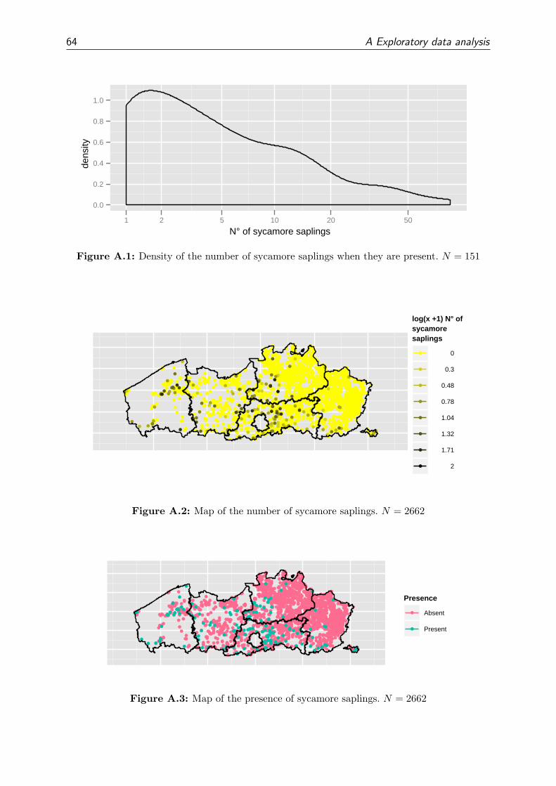
64 A Exploratory data analysis
N° of sycamore saplings
dens
ity
0.0
0.2
0.4
0.6
0.8
1.0
1 2 5 10 20 50
Figure A.1: Density of the number of sycamore saplings when they are present. N = 151
●●●● ●
●●●●●●●●●●●●●●●●●●●●●
●●● ●
●●●●●●
●
●●●●●●●●●●●●●●●●● ●●●● ●●●● ●●●
●●
●●●●●●●●●●●●
●●●●●●●●●●●●●●●●●●● ●●●●●●●●●●●●●●●●●● ●●●●●●●●●●●●●●●●●●
●●●●●●●●●●●●
●●
●●●●●●●●●●●● ●●● ●●● ●●●
●●●●●●●●●●●●●●●●●●●●●●●●●●●●●●●●●●●●●●●●●●●●●● ●●●●●
●●●●●●●●●●●●●●
●●●●● ●●● ●●●● ●●●●●●●●●●●●●●●●●●●●●●●●
●●● ●●●●● ●●●●●● ●●●●●● ●●●●●●● ●
●●● ●● ●●●●●●●●●●●●●●●●●●●●●●●●●●●●●● ●●●●●●●●●●●●●●●●●●●●●●●●●●●●●●●● ●●●●
●●● ●●●●●●●●●●●●●●●●●●●●●● ●●● ●●●●●●● ● ●●●●●●●●●●●●
●●●●●●
●●●●●●●●●● ●●●●●●●● ●
● ●● ●● ●
●●●● ●
●●●●●●●●● ●●●
●●
●●●●●● ●●● ●●● ●●
●●●●●●●●●●●●● ●● ●●●●● ●●●●
●●
●● ● ●●●
●●● ●●●●●●
●●● ●●●●●●●● ●● ●●● ●●●●●●●●●
●●
●●●●●●●● ●●●●●
●● ●●● ●●●●●●●●
●●●●●●●●●
●● ●●●● ●●●●
●●●●●●●
●●● ●●●●●●●●● ●●●●●● ●●●● ●●
●● ●●●●●●●●
●● ●●●
●● ●●●●● ●●●●●●●●●●●●●● ●●●●●●
● ●●● ●●●●●● ●●●●●●● ●● ●●●●●●●●●●●●●●●●●●●● ●●●
●●●●●●●●●●●● ●●●●●●● ●●●●●●●●●●●●●●●●●●
●●●●●●●●●●●●●●●● ●●●●●●●●●●●●●●
●
●●●●●●●● ●●●●●●●●●●●●
●●●● ●●●●●●●●●●●●●●●●
●●●●● ●●●●●● ●●●●●
●●●●●●●●●●●● ●●●●●●●●●●
●●●●●●●●●● ●●●●●●●●●●●● ●●●●●●●●●●●●●●
●●●●●●● ●●●●●●●●●●●● ●●●●●●●●●●●●●●●●●●●● ●●●● ●
●●●●●●●● ●●● ●●●●● ●●●●●●●●●●●●●●●● ●●●●● ●●●●●●●●●●● ●●●●●●●●●●●●
●●● ●●●●●●●●●● ●●●● ●● ●●●●●●●●●● ●●●●
● ●●●●● ●●●●●●●●●●●● ●●●● ●●● ●●●●●●●●●●●●●●●●●●●●●●●●●
●● ●●●●●●●●●● ●●●●● ●● ●● ●●●●●●●●●●●●●●●●●●● ●●
●●●●●●●●●●●●●●●●●●●●●●●● ●●●●●●●●●●●●●●●
●●●●●●●●●●●●●●●●●●●●●●●●●● ●●●● ●●●●●●
●●
●●●●●●●●●● ●●● ●●●
●●● ●●●●●●●●●●●●●●●●●●●
●
●● ●●● ●● ●●● ●
●●
●●●●
●●●
● ●●● ● ●● ●●●● ●●●●
●●●
●●
●●
●
●●
●●● ●
●●●●
●●●●
●
●●●
●●●●●●
●●●●●●●●●●● ●
●●● ●●● ●●
●●
●●●●●●
●●●●●●●●●● ●●
●● ●●●●●●
●●
●●●●●●●●●●
●●●●●●● ●●●
●●●●●●●
●●●● ●●●● ●
●●● ●●●●●●●●●●●●●
●●●●●●●●●
●●●●●
● ●
● ●●●● ●●●●●●●●● ●●●●● ●●●●●●●●●
●●●●●●●●●●●●●●● ●●●●●●●●●●●●●● ●● ●●●●●●●●●●●●●● ●●● ●● ●●
●●●● ●●●● ●● ●●●●●●●●●●●●●●●●●●
●●●●●●●● ●● ●● ●● ●●●●●●●● ●●● ●●● ●●● ●●
●●● ●●●● ●
● ●●●●●●●●●●●●● ●●● ●●●●●●●● ●● ●●●●●●●●●●●●●●
●●● ●●● ●●●● ●●●●●●●●●●●
●● ●●●●●●●●●●● ●●●●●●● ●● ●●● ●● ●●●●●●●●●●●●●
●●●●●●●●●●● ●●● ●●●●●●●●●●●●● ●●● ●●●●●●●●●●●●●●● ●● ●●●●●● ●● ●●●●●
● ●●●●●●●●● ●●●●●●
●●●●●●●●●●● ●●● ●●●●● ●● ●●●●●●●●●
●●●●●●●●●●●● ●●●●●●●●
●●●●●●●● ●● ●●●●●●●●●●●●●●●●● ●●●●●●●●●●●●●●●●● ●●● ●●●●●
●●●●●●●●●●●●●●●●●●●●●●● ●●●●●●●●●●●●●●●●●● ●●●● ●●●●●●●●●●●●●●●●●●●●●●
●● ●●●●●●●●●●●●●●●●●●●●●● ●●●●●●●●●●●●●●● ●●●●●●●●●●●●● ●●● ●●●●●●●●●●
●●●●●●●●●●●● ●●●● ●●●●●●●●●●●●●●●●●●●●●●●●●●●●●●●●●●●●●●●●●●●●●●●●● ●●●●● ●●●●●●●●●●●●●●●●●●●●●●
●
●●●
●●●
●
●●●
●●●● ●
●●● ●●●●●
●●●●●●●
●●●●●●●
●●●
●●
●●●
●●
●●● ●●● ●●●●●●● ●
●● ●●●
●●● ●
●●●●●● ●●●● ●●● ●
●●●●●●●
●●●●●●●●●●●● ●●●●
●●●●●●●
●●●●●●●●●
●●● ●●
● ●●●●●●●● ●●●●●●● ●●●●●●●●●●
●●●●●●●●●●●●●●●●●●●●●● ●●●●●●●●●●
●● ●●●●●●●●●●
●●●●●●
● ●● ●●● ●●●●● ●●●●● ●
●●●●●●● ●● ●●●●
●●● ●●
●●●●●●●●●●●●● ●●●●●●●●
●●●●●●●●●●●●●●●●●●●●●●●●● ●● ● ●●
●●●●
●●
●●●●●● ●●●●●●● ●● ●●
●●● ●●●●●
●●●●●●●●●●●●● ●● ●●
●●●●●●
●
● ●●● ●●●●● ●●●●●●● ●
●●●●●●●●●●●●●●●● ●●●●
●●●●●●●●●●●●
●●●●●●● ●●● ●●●●●●●●●●●●
●● ●●●●●●●●●●●●●●●●● ●
●
● ●
●●
●●
●
●●
●●
●
●
●
●● ● ●
●
●●
●●
●
●●●● ●●
●
●
●●
●
●● ●
●
●
●●●
●
●●
●
●●
●
●●
●●● ● ●●
●●
●
●
●
●
●
●
● ● ●
● ●
●●
●
●
● ●●
●
● ● ●
●
●
●●
●
●●
●●
●
●
●
●
●
●
●
●
●
●
●
●
●●
●
●
●
●
●
●
●
●
●
●
● ●
●
●
●
●
●
●
●
●
●
●
●
●
●
●
●
●
●●
●●
●
●●
●●
●
●
●●
●
●
●●
log(x +1) N° ofsycamoresaplings
● 0
● 0.3
● 0.48
● 0.78
● 1.04
● 1.32
● 1.71
● 2
Figure A.2: Map of the number of sycamore saplings. N = 2662
● ●●● ●●●●●●●●●●●●●
●●●●●●●●●
●●● ●
●●●●●●●
●●●●●●●●●●●●●●●●● ●●●● ●●●● ●●●
●●
●●●●●●●●●●●●
●●●●●●●●●●●●●●●●●●●●●●●●●●●●●●●●●●●●●●●●●●●●●●●●●●●●●●●
●●●●●●●●●●●●
●●
●●●●●●●●●●●●●●● ●●●●●●
●●●●●●●●●●●●●●●●●●●●●●●●●●●●●●●●●●●●●●●●●●●●●● ●●●●●
●●●●●●●●●●●●●●
●●●●● ●●● ●●●● ●●●●●●●●●●●●●●●●●●●●●●●●
●●●●●●●● ●●●●●● ●●●●●● ●●●●●●●●
●●● ●●●●●●●●●●●●●●●●●●●●●●●●●●●●●●●● ●●●●●●●●●●●●●●●●●●●●●●●●●●●●●●●● ●●●●
●●● ●●●●●●●●●●●●●●●●●●●●●●●●● ●●●●●●● ● ●●●●●●●●●●●●
●●●●●●
●●●●●●●●●● ●●●●●●●● ●
● ●● ●● ●
●●●●●
●●●●●●●●●●●●
●●●●●●●●●●●●●●●●
●●●●●●●●●●●●●●●●●●●●●●●●
●●
●● ● ●●●●●●●●●●●●
●●●●●●●●●●● ●● ●●●●●●●●●●●●
●●
●●●●●●●● ●●●●
●
●● ●●● ●●●●●●●●
●●●●●●●●●
●●●●●● ●●●●
●●●●●●●
●●● ●●●●●●●●●●●●●●●●●●● ●●
●●●●●●●●●●
●●●●●
●●●●●●●●●●●●●●●●●●●●●●●●●●●
● ●●●●●●●●●●●●●●●●●● ●●●●●●●●●●●●●●●●●●●●●●●
●●●●●●●●●●●●●●●●●●● ●●●●●●●●●●●●●●●●●●
●●●●●●●●●●●●●●●● ●●●●●●●●●●●●●●
●
●●●●●●●● ●●●●●●●●●●●●
●●●● ●●●●●●●●●●●●●●●●
●●●●● ●●●●●●●●●●●
●●●●●●●●●●●●●●●●●●●●●●
●●●●●●●●●● ●●●●●●●●●●●● ●●●●●●●●●●●●●●
●●●●●●●●●●●●●●●●●●● ●●●●●●●●●●●●●●●●●●●● ●●●● ●
●●●●●●●● ●●● ●●●●● ●●●●●●●●●●●●●●●● ●●●●●●●●●●●●●●●●●● ●●●●●●●●●●
●●● ●●●●●●●●●●●●●● ●● ●●●●●●●●●●●●●●
●●●●●●●●●●●●●●●●●●●●●● ●●● ●●●●●●●●●●●●●●●●●●●●●●●●●
●●●●●●●●●●●●●●●●● ●● ●●●●●●●●●●●●●●●●●●●●●●●
●●●●●●●●●●●●●●●●●●●●●●●●●●●●●●●●●●●●●●●●●●●●●●●●●●●●●●●●●●●●●●●●●●●●●●●●●●●
●●●●●●●●●●●●●●●●●●
●●● ●●●●●●●●●●●●●●●●●●●
●
●● ●●● ●● ●●● ●
●●
●●●●
●●●
● ●●● ● ●● ●●●● ●●●●
●●●●●
●●●
●●
●●● ●●●●●
●●●●
●
●●●
●●●●●●
●●●●●●●●●●●●
●●●●●●●●●●
●●●●●●
●●●●●●●●●● ●●
●● ●●●●●●
●●
●●●●●●●●●●
●●●●●●● ●●●
●●●●●●●
●●●●●●●● ●
●●● ●●●●●●●●●●●●●
●●●●●●●●●
●●●●●● ●
● ●●●●●●●●●●●●● ●●●●● ●●●●●●●●●
●●●●●●●●●●●●●●●●●●●●●●●●●●●●● ●● ●●●●●●●●●●●●●●●●●●●●●
●●●● ●●●● ●●●●●●●●●●●●●●●●●●●●
●●●●●●●●●● ●●●● ●●●●●●●●●●● ●●● ●●● ●●
●●● ●●●● ●
● ●●●●●●●●●●●●● ●●●●●●●●●●● ●●●●●●●●●●●●●●●●
●●●●●●●●●●●●●●●●●●●●●
●●●●●●●●●●●●● ●●●●●●●●●●●● ●●●●●●●●●●●●●●●
●●●●●●●●●●● ●●●●●●●●●●●●●●●● ●●●●●●●●●●●●●●●●●●●● ●●●●●●●● ●●●●●
● ●●●●●●●●● ●●●●●●
●●●●●●●●●●●●●● ●●●●●●● ●●●●●●●●●
●●●●●●●●●●●●●●●●●●●●
●●●●●●●●●●●●●●●●●●●●●●●●●●●●●●●●●●●●●●●●●●●●●●● ●●●●●
●●●●●●●●●●●●●●●●●●●●●●● ●●●●●●●●●●●●●●●●●● ●●●●●●●●●●●●●●●●●●●●●●●●●●
●● ●●●●●●●●●●●●●●●●●●●●●●●●●●●●●●●●●●●●●●●●●●●●●●●●●● ●●● ●●●●●●●●●●
●●●●●●●●●●●●●●●●●●●●●●●●●●●●●●●●●●●●●●●●●●●●●●●●●●●●●●●●●●●●●●●●●●●●●● ●●●●●●●●●●●●●●●●●●●●●●
●
●●●
●●●
●
●●●
●●●● ●
●●● ●●●●●
●●●●●●●
●●●●●●●
●●●●●
●●●
●●
●●●●●● ●●●●●●● ●
●●●●●
●●● ●
●●●●●●●●●● ●●● ●
●●●●●●●
●●●●●●●●●●●●●●●●
●●●●●●●●●●●●●●●● ●●● ● ●
● ● ●●●●●●●●●●●●●● ●●●●●●●●●●
●●●●●●●●●●●●●●●●●●●●●●●●●●●●●●●●
●●●●●●●●●●●●
●●●●●●● ●● ●●● ●●●●● ●●●●●●
●●●●●●● ●● ●●●●
●●●●●
●●●●●●●●●●●●● ●●●●●●●●
●●●●●●●●●●●●●●●●●●●●●●●●● ●● ●●●
●●●●
●●
●●●●●●●●●●●●● ●● ●●
●●●●●●●●
●●●●●●●●●●●●● ●● ●● ●
●● ●●●●
●●●●●●●●●●●●●●●● ●
●●●●●●●●●●●●●●●●●●●●
●●●●●●●●●●●●
●●●●●●● ●●● ●●●●●●●●●●●●
●● ●●●●●●●●●●●●●●●●● ●
●
● ●
●●
●●
●
●●
●●
●
●
●
●● ● ●
●
● ●
● ●
●
●●●● ●●
●
●
●●
●
●● ●
●
●
●●●
●
●●●
●●
●
●●
●●● ● ●●●
●
●
●
●
●
●
●
● ● ●
● ●
●●
●
●
● ●●
●
● ● ●
●
●
● ●●
●●
●●
●
●
●
●
●
●
●
●
●
●
●
●
● ●
●
●
●
●
●
●
●
●
●
●
● ●
●
●
●
●
●
●
●
●
●
●
●
●
●
●
●
●
●●
● ●
●
● ●
●●
●
●
●●
●
●
●●
Presence
● Absent
● Present
Figure A.3: Map of the presence of sycamore saplings. N = 2662

A.1 Natural regeneration of sycamore 65
●●● ●●●●●●●●●●
●
● ●● ●●●
●
●
●●●●●●●● ●● ●●●●●● ●● ●● ●●●●●● ●●●●●● ●● ●● ●● ●● ●●●● ●● ●
●●●●● ●●
●●●●●●
●●●●● ●●●●●
●●
●●●●
●●●●●●
●●●●●●●●
●●●●
●●●
●●●
● ●●●●
● ●●●
●●●●●
●●●
●●●●●●●●
●● ●●● ●● ●
● ●●●
● ●
●●
●●●
● ● ●●
●●
●
●●●● ●●●●●●●●
● ●●●●●●●●
●●
●●●●
●●●● ●●●●●●
●●
●●●●●●●●●●●●●
●
● ●●●●●●●●●●●●●●●
●●
●● ●●●●●●●●●●●●
●●
●●●●●●●●●●●●●●
●
●
●●●●●●●
●●●●●●
●●
●●
●● ●●●●●●●●●●●●● ●●●●●● ●● ●●●● ●●●●●● ●●●●●●●●●● ●● ●●●
●●
●● ●●●●
●●●●●●●●●
●●● ●●
●●● ●● ●
●●●●●●● ●
● ● ●●●
●●●●
●●●●
●●●●
●●●●●●
●●●●●
● ●●● ●
●
● ●● ● ●
● ●● ●● ●● ●●●●
● ●
●●●●●●●●
●●●●●●●●●●●●●●●●●●●●● ●●●●●●
●●●●
●●●●●●●●●●●
●● ●● ●● ●●●●●●●●
●
●
●●●●●●●●●●●●●●
●●
●●●●●●●●●●●●●
●●
●●●●● ●●●●●●●●
●
●
●●●● ●●●●●●●●●●
●●
●●
●●●●●●●●●● ●●●● ●●●●●● ●●●● ●●●●●●●●●● ●●●●●●●●●●●● ●● ●
●
●●●●
●●●●
● ●●●
● ●●●
● ●●●
●●●●●
●●●●●●●●●●
●●● ●● ●
●●
●●●●●●
●●●●●●
● ●●●
●●● ●●
●●
●●●●
●● ●
●● ●
● ● ●
● ●● ●●●●
●●●
●● ●● ●●
●●●●●●●●●●●●●
●●●●●
●●●● ●
●●●●●
●●●●●●●●
●●●● ●●●
●●●●●●●
●●●● ●●●●●●●●●
●●●
●●●●●
●●●●
●●●●●●●●●●●●●
●●
●●●● ●
●●●● ●●●●●●●●●●● ●●●●●●●●●●●● ●●●●●●
●● ●
●
●●●●
●●● ●●●
●●●●●●●●● ●
●●●●
●●●
●●●●●●●●●●●●
● ●
●●●●●●●●
●●●●●
●●●
●●●
● ●●● ●●●●
●
Onderzochtehokken
● 0
● 4
● 8
● 12
● 16
Ratio
● 0
● 0.2
● 0.4
● 0.6
● 0.8
● 1
Figure A.4: Ratio of the number of 1x1 km grid cells with presence of sycamore and the numberof visited 1x1 km grid cells in each 4x4 km grid cell (Van Landuyt et al., 2006).N = 905

66 A Exploratory data analysis
A.2 Regions
As the distribution of sycamore saplings seems to differ between regions, we look at the
ecological regions as a relevant division (Sevenant et al., 2002). This is available as GIS
layers covering the entire study area (Flanders).
The saplings are present in most of the ecoregions except the Kempen and the Grindriv-
ieren (fig. A.5). The number of saplings exhibits much more differentiation (fig. A.6).
The natural regeneration of sycamore differs between the ecoregions. Therefore we
think that the analysis will benefit from a stratification or random effect based on ecore-
gion.
Ecological region
Pro
babi
lity
0.1
0.2
0.3
0.4
0.5
0.6
●
● ●
●
●
●●
●
●
●
●
Cue
stas
Grin
driv
iere
n
Kem
pen
Krij
t−le
emge
bied
en
Krij
tgeb
iede
n
Mid
den−
Vla
amse
ove
rgan
gsge
bied
en
Ple
isto
cene
riv
ierv
alle
ien
Pol
ders
en
de g
etijd
ensc
held
e
Wes
telij
ke in
terf
luvi
a
Zui
doos
telij
ke h
euve
lzon
e
Zui
dwes
telij
ke h
euve
lzon
e
Figure A.5: Probability of sycamore saplings per ecological region.

A.3 Geomorphology 67
Ecological region
Log1
0 nu
mbe
r of
sap
lings
−0.2
−0.1
0.0
0.1
0.2
0.3
0.4
●
● ●
●
●●
●●
●
●●
Cue
stas
Grin
driv
iere
n
Kem
pen
Krij
t−le
emge
bied
en
Krij
tgeb
iede
n
Mid
den−
Vla
amse
ove
rgan
gsge
bied
en
Ple
isto
cene
riv
ierv
alle
ien
Pol
ders
en
de g
etijd
ensc
held
e
Wes
telij
ke in
terf
luvi
a
Zui
doos
telij
ke h
euve
lzon
e
Zui
dwes
telij
ke h
euve
lzon
e
Figure A.6: Average log10 number of sycamore saplings in a plot per ecological region
A.3 Geomorphology
The altitude and slope are based on a digital elevation model with a 25×25m grid covering
Flanders (Ondersteunend Centrum GIS-Vlaanderen, 2004).
� Fig. A.7 and A.8 show a linear to quadratic relationship between the altitude and
both the presence and the number of saplings.
� The relationship with the slope is rather linear (fig. A.9 and A.10).
Altitude
Pro
babi
lity
of s
aplin
gs
0.0
0.2
0.4
0.6
0.8
1.0
● ●●●● ●●●●●●●●●● ●●●●●●●●●● ●●●●●●●●●●●● ●●●● ●●●●●●●●●● ●● ●●●● ●● ●● ● ●●●●●●●● ●●●●●●●●●●●●●●●●● ●●●●●●●●●●●●●●●● ●●●●●●●●● ●●●●●● ●●●●●●●●●● ●●●●●●● ●●●●●● ●●●● ●●●●●● ●●●●●●●●●●●●●●●●●●●●●●●● ●●●●● ● ●●●●●●●●●●● ●●●●●●●●●●●●●●●●●●●●●●●●●●● ●●●●● ●●●●●●●●●●●●●●● ●●●●●●●●●●●●●●●●●●●●●●●●●●●●●●●●●●●●●●●●●●●●●●●●●●●●●●●●●●●●●●●●● ●●● ●●●●●● ●●●●●● ●●●● ●● ●●● ●●● ●● ●●●●●●●●●●●●● ●●● ●●●●●●●●● ● ●●●●●● ●●●●●●● ●●●●●●●● ●●●●●●●● ●●●●●●●●●●● ●●●●●●● ●● ●● ●●●●● ●●●●●●●●●●●●●●●●●●●●●●●●● ●● ●●●●●●● ●●●●●●●●●●●●●●●●●●● ●●●●●● ●● ●●●●●● ●● ●●●●●● ●●●●●● ●●●●●●●●●●●●●●●●●●●●●●● ●● ●● ●●●●●●●●●●●●●●●●●●●●●●●●● ●●●●●●●●●●●●●●●●●●●●●●● ●●●●●●●●●●●● ●●●●●●●●●●●●●● ●●● ●● ● ●● ●● ●● ●●●● ●●●●●●●●●●●●●●●●●●●●●●●●●●● ●●●●●●●●●●●●●●● ●●●●●●●●●● ●●●●●●●●●●●●●●●● ●●●● ●●● ●●●● ● ●● ●●●●●●● ● ●●●●●●●●●●●●●●● ●●●●●●●●●●●●●●●●● ●●●● ●●● ●●●●●●●●●● ●●●●●●●●● ●●●●● ●●●●● ●●●●● ●●●●●● ●●●● ●●● ●●●● ●●●●●●●●●●● ●● ●●●●● ●●●●●●●●●●●●●●●●●●●●●●●●●●●●●●●●●●● ● ●●●●●●●●●●●●●●●●● ●●●●●● ●●●● ●●●●●●●●●●●●●● ●●● ●●●●●●●●● ●● ●●●●●● ●●● ●● ● ●● ●● ●● ●● ●●●●●●●●●●●●●●●●●●●●●●●●●●●● ●●●●●●●● ●●●● ● ●● ●●●●● ●●●●●●●●●● ●●●●●●●●●●●● ●●●● ●●●●● ●●● ●● ●●●● ●● ● ● ●●● ●● ●●● ● ●● ● ● ●●●●●●●●● ●●●● ●●●●● ●● ●●●●●●●●●●●●●●●●●● ●● ●●●●●● ●●● ●● ●●●● ●●●●●●●●●●● ●● ●●●●●●● ●●●●●●●●●●●●●●●●●●●●●●●●●●●● ● ●● ●● ●●●●●● ●●● ●●●● ●●● ●●●●● ●●●●●●●●●●●●●●●●●●●●●●●●●●●●●● ●●● ●●●●●●●●● ● ●●●● ● ●● ●●● ● ●●●●● ●●●●● ●●● ● ●●● ●● ●●●● ●●●● ●● ● ●●●● ●● ●● ●●●●●●● ●● ●● ●●●● ●● ● ●●●●● ●● ●● ●●●●●●● ●● ●● ●●●●● ●● ●●●● ●● ●●●● ●● ●●● ● ●● ● ●● ●●●● ● ●●●● ●●●● ●● ● ● ●●●●●●● ●●●●●●●●● ●●●● ●●●● ●●●●●●● ●● ●●●●●● ●● ●●●● ●●●● ●●● ●●● ● ●●●●●●●●●●●●●●●●●●●●●●●●● ●●●●● ●●●●●● ●●●● ●● ●●● ●●●●●● ●●●●●● ●● ●●●● ●●● ●●●● ●● ●●●●●● ● ●●● ●●●●●● ● ●● ●●●● ●●●● ●●●●●● ●● ●●● ●●●● ●● ●●● ●●●● ●●●●● ●●● ●● ●● ● ●●●● ● ●●●●● ●●●● ●●● ●●●●● ●●●●● ●●●●●● ●●●●● ●● ●●● ●●●●●●●● ●●●● ●● ●●●● ● ●●●●● ●●●●● ●●●● ● ● ●●● ●●●●●●●●● ● ●●● ● ● ●● ● ●●● ●● ●●●● ●● ● ●●●● ●● ●●●● ●●● ●●● ● ●●●● ● ● ● ●● ●●●●●●●●●●● ●●●● ●● ●●● ●●●● ●● ●●● ●●●●●● ●●● ●● ●●●● ●●● ●●● ●● ● ●● ●●● ● ●●● ●●●●● ●● ● ● ● ●●● ●● ●●●●● ●●●●● ●●● ●●● ●●● ●●● ●●●● ●● ●● ●● ●●● ●● ●● ●● ●●● ● ●●●●● ●● ●● ●●●●●● ●●●● ●● ●● ●●● ●●● ● ● ●●● ●●● ●● ●● ●●●● ●● ●●● ●● ●●● ●●●● ●●●●●●● ●● ●● ●●● ●●●●● ●●●●●● ●●● ●●●● ●●● ●●● ●● ●●●●●● ●● ● ●●● ●●●● ● ●●● ● ●● ●●●● ● ●● ●●●●● ●●● ●●● ●●● ●● ●●●●● ●●● ●●●●● ● ●● ●●● ●● ●●● ● ● ●● ●●● ●● ●●● ●●● ●●● ●●● ● ●● ●●●●●●●●●●●●● ●●●●●●●●●●●●●●●●●● ●●●●● ●●●●●●●●●●●●●●●●●●●●●●●●●●●● ●●●●●●●●●●●●●●●●●●●●●●●●●●●●●●●●●●●●●●●●●●●●●●●●●●●●●●●●●●●●●●●●●● ●●●●●●●●● ●●●●●●● ●●●● ●●●●●●●●●●●●●●●● ●●●●●●●●●●● ●●●●●●●●●●● ●● ● ●●●●●●●●●●●●● ● ●●●● ●●●● ●●●●●●●● ● ●●●●●●● ●● ●●● ●● ●●● ●● ●●● ●●●●● ● ● ●●●● ●●●● ●●●●
●● ●● ●●●●●● ●●● ●● ●● ●● ●●●●●● ●● ●●● ●● ● ●● ●● ●● ● ●● ●● ● ●●● ● ●●●● ● ●●●●●●● ●● ●● ● ●● ●● ●●● ●●● ●● ● ●●●●●● ●● ●●● ● ●●● ●● ● ● ●●●● ●● ●●● ● ●●● ●● ● ●●● ●●● ●●● ● ●● ●●● ●●● ● ●●●● ● ●● ●●● ●●● ●●●●●
50 100 150 200 250
Figure A.7: Probability of sycamore saplings with regard to the altitude.

68 A Exploratory data analysis
Altitude
Log1
0 nu
mbe
r of
syc
amor
e sa
plin
gs
0.0
0.5
1.0
1.5
● ●●●● ●●●●●●●●●● ●●●●●●●●●● ●●●●●●●●●●●● ●●●● ●●●●●●●●●● ●● ●●●● ●● ●● ● ●●●●●●●● ●●●●●●●●●●●●●●●●● ●●●●●●●●●●●●●●●● ●●●●●●●●● ●●●●●● ●●●●●●●●●● ●●●●●●● ●●●●●● ●●●● ●●●●●● ●●●●●●●●●●●●●●●●●●●●●●●● ●●●●● ● ●●●●●●●●●●● ●●●●●●●●●●●●●●●●●●●●●●●●●●● ●●●●● ●●●●●●●●●●●●●●● ●●●●●●●●●●●●●●●●●●●●●●●●●●●●●●●●●●●●●●●●●●●●●●●●●●●●●●●●●●●●●●●●● ●●● ●●●●●● ●●●●●● ●●●● ●● ●●● ●●● ●● ●●●●●●●●●●●●● ●●● ●●●●●●●●● ● ●●●●●● ●●●●●●● ●●●●●●●● ●●●●●●●● ●●●●●●●●●●● ●●●●●●● ●● ●● ●●●●● ●●●●●●●●●●●●●●●●●●●●●●●●● ●● ●●●●●●● ●●●●●●●●●●●●●●●●●●● ●●●●●● ●● ●●●●●● ●● ●●●●●● ●●●●●● ●●●●●●●●●●●●●●●●●●●●●●● ●● ●● ●●●●●●●●●●●●●●●●●●●●●●●●● ●●●●●●●●●●●●●●●●●●●●●●● ●●●●●●●●●●●● ●●●●●●●●●●●●●● ●●● ●● ● ●● ●● ●● ●●●● ●●●●●●●●●●●●●●●●●●●●●●●●●●● ●●●●●●●●●●●●●●● ●●●●●●●●●● ●●●●●●●●●●●●●●●● ●●●● ●●● ●●●● ● ●● ●●●●●●● ● ●●●●●●●●●●●●●●● ●●●●●●●●●●●●●●●●● ●●●● ●●● ●●●●●●●●●● ●●●●●●●●● ●●●●● ●●●●● ●●●●● ●●●●●● ●●●● ●●● ●●●● ●●●●●●●●●●● ●● ●●●●● ●●●●●●●●●●●●●●●●●●●●●●●●●●●●●●●●●●● ● ●●●●●●●●●●●●●●●●● ●●●●●● ●●●● ●●●●●●●●●●●●●● ●●● ●●●●●●●●● ●● ●●●●●● ●●● ●● ● ●● ●● ●● ●● ●●●●●●●●●●●●●●●●●●●●●●●●●●●● ●●●●●●●● ●●●● ● ●● ●●●●● ●●●●●●●●●● ●●●●●●●●●●●● ●●●● ●●●●● ●●● ●● ●●●● ●● ● ● ●●● ●● ●●● ● ●● ● ● ●●●●●●●●● ●●●● ●●●●● ●● ●●●●●●●●●●●●●●●●●● ●● ●●●●●● ●●● ●● ●●●● ●●●●●●●●●●● ●● ●●●●●●● ●●●●●●●●●●●●●●●●●●●●●●●●●●●● ● ●● ●● ●●●●●● ●●● ●●●● ●●● ●●●●● ●●●●●●●●●●●●●●●●●●●●●●●●●●●●●● ●●● ●●●●●●●●● ● ●●●● ● ●● ●●● ● ●●●●● ●●●●● ●●● ● ●●● ●● ●●●● ●●●● ●● ● ●●●● ●● ●● ●●●●●●● ●● ●● ●●●● ●● ● ●●●●● ●● ●● ●●●●●●● ●● ●● ●●●●● ●● ●●●● ●● ●●●● ●● ●●● ● ●● ● ●● ●●●● ● ●●●● ●●●● ●● ● ● ●●●●●●● ●●●●●●●●● ●●●● ●●●● ●●●●●●● ●● ●●●●●● ●● ●●●● ●●●● ●●● ●●● ● ●●●●●●●●●●●●●●●●●●●●●●●●● ●●●●● ●●●●●● ●●●● ●● ●●● ●●●●●● ●●●●●● ●● ●●●● ●●● ●●●● ●● ●●●●●● ● ●●● ●●●●●● ● ●● ●●●● ●●●● ●●●●●● ●● ●●● ●●●● ●● ●●● ●●●● ●●●●● ●●● ●● ●● ● ●●●● ● ●●●●● ●●●● ●●● ●●●●● ●●●●● ●●●●●● ●●●●● ●● ●●● ●●●●●●●● ●●●● ●● ●●●● ● ●●●●● ●●●●● ●●●● ● ● ●●● ●●●●●●●●● ● ●●● ● ● ●● ● ●●● ●● ●●●● ●● ● ●●●● ●● ●●●● ●●● ●●● ● ●●●● ● ● ● ●● ●●●●●●●●●●● ●●●● ●● ●●● ●●●● ●● ●●● ●●●●●● ●●● ●● ●●●● ●●● ●●● ●● ● ●● ●●● ● ●●● ●●●●● ●● ● ● ● ●●● ●● ●●●●● ●●●●● ●●● ●●● ●●● ●●● ●●●● ●● ●● ●● ●●● ●● ●● ●● ●●● ● ●●●●● ●● ●● ●●●●●● ●●●● ●● ●● ●●● ●●● ● ● ●●● ●●● ●● ●● ●●●● ●● ●●● ●● ●●● ●●●● ●●●●●●● ●● ●● ●●● ●●●●● ●●●●●● ●●● ●●●● ●●● ●●● ●● ●●●●●● ●● ● ●●● ●●●● ● ●●● ● ●● ●●●● ● ●● ●●●●● ●●● ●●● ●●● ●● ●●●●● ●●● ●●●●● ● ●● ●●● ●● ●●● ● ● ●● ●●● ●● ●●● ●●● ●●● ●●● ● ●● ●●●●●●●●●●●●● ●●●●●●●●●●●●●●●●●● ●●●●● ●●●●●●●●●●●●●●●●●●●●●●●●●●●● ●●●●●●●●●●●●●●●●●●●●●●●●●●●●●●●●●●●●●●●●●●●●●●●●●●●●●●●●●●●●●●●●●● ●●●●●●●●● ●●●●●●● ●●●● ●●●●●●●●●●●●●●●● ●●●●●●●●●●● ●●●●●●●●●●● ●● ● ●●●●●●●●●●●●● ● ●●●● ●●●● ●●●●●●●● ● ●●●●●●● ●● ●●● ●● ●●● ●● ●●● ●●●●● ● ● ●●●● ●●●● ●●●●
●● ●● ●●●●●● ●●● ●● ●● ●● ●●●●●● ●● ●●● ●
● ● ●● ●● ●● ● ●● ●● ● ●●● ● ●●●● ● ●●●●●●● ●● ●● ● ●● ●● ●
●● ●●● ●● ● ●●●●●● ●● ●●● ● ●
●● ●● ● ● ●●●● ●● ●●● ● ●●● ●● ● ●●● ●●● ●●● ● ●● ●●● ●●● ● ●●●● ● ●● ●●● ●●● ●●●
●●
50 100 150 200 250
Figure A.8: Log10 number of sycamore saplings with regard to the altitude.
Slope
Pro
babi
lity
of s
aplin
gs
0.0
0.2
0.4
0.6
0.8
1.0
● ● ●● ●● ●● ● ●● ●● ●●●●● ●●● ●● ● ●● ●● ●● ● ●● ●● ●● ●●● ●● ● ●●● ●●● ● ●●● ●● ●● ● ● ● ●●●● ●●● ● ● ● ●● ●● ●●●● ●● ●●● ●● ● ●● ● ●● ●● ● ● ●● ● ●● ● ● ●●● ● ●●● ●● ●● ●●● ●● ●● ●● ●● ●● ● ●● ●● ●● ● ● ● ●●●●● ● ● ●●●● ● ●● ●●● ●●●● ● ●● ●●● ●●● ●● ●● ●● ● ●●●● ●●● ●● ●●● ●● ●● ● ●● ●●● ● ● ●● ●● ● ●●● ●● ●●● ●●●●● ● ●●●● ● ●● ●● ● ●● ● ●● ●●● ●●● ●● ●● ●● ●● ●●●● ●● ● ●●● ●● ●●● ●●● ● ●● ●●● ● ●● ●● ●●●● ●● ●● ●●● ●●● ● ●● ●● ●● ● ●● ● ●●● ●● ●● ●●● ●●● ●● ●●●● ●● ●● ●● ●● ●●●● ●● ● ●●●● ● ●●●● ● ● ●● ●● ● ●●● ●●●●● ● ●●● ●● ●● ●●●●● ●● ●● ● ●●● ●● ●● ●● ●● ●● ●●● ●● ●● ●● ●● ●●●● ● ● ●● ● ●●●● ● ●● ●●● ●● ●● ●●● ●● ●●●●● ●● ●● ● ● ●● ●● ●● ●● ●●● ●● ●● ●● ●●● ● ●● ● ●●●● ● ●●●● ● ●●● ● ●● ●●● ●●● ●● ● ●● ●● ●● ●●● ●● ●● ● ● ●●● ● ●● ● ●●● ● ●●● ● ●● ●● ● ●●●●● ● ●● ●● ●● ● ●●●● ●● ●●● ●● ●● ● ●●● ●● ● ●●●● ●● ● ●● ●●● ●● ● ● ●●● ●● ●● ●●●●● ● ●●●● ●●● ●●● ● ●● ●● ●● ● ● ●● ●● ●●● ●●● ●● ● ●● ●● ● ● ●● ● ●● ● ● ●● ● ●● ●●● ●● ●● ●●● ●●● ●● ●● ● ●● ● ●● ●●● ● ●● ●● ●● ● ●●● ● ● ●●● ● ●●● ●● ●● ●●● ●● ●● ●●● ●● ●●● ●● ● ●● ●●● ●● ● ●● ● ● ●● ●●● ●● ●●● ●● ●● ●●●●● ● ●● ●● ● ●●● ●●●● ●●● ●●● ● ●● ● ●● ●● ●● ● ● ●● ●● ●●● ● ●● ● ●●● ●● ●● ● ● ●● ●● ●● ●● ● ●●● ●● ●● ●●● ●●●● ●● ●● ●●●● ●●●● ●●● ●● ● ●● ● ●● ● ●●● ●●● ● ●●●● ●● ● ●●●● ● ● ●●●● ● ●● ●●● ●●● ●● ● ● ●● ● ● ●● ●● ● ●● ● ●● ● ●●●●● ●● ●●● ● ● ●●●●● ● ●●●● ● ●●●● ● ●●●● ●● ●● ●● ●●● ●●●● ●● ●●● ●● ● ● ●● ●● ●●●● ● ●● ● ● ●● ● ●●● ●● ●● ●● ● ● ●● ● ●● ● ● ● ●● ●● ●●● ● ●●● ●●● ● ● ● ●● ● ●●● ● ●●●● ● ●●● ● ●●● ● ●●● ●●● ●● ●● ●●● ● ●● ● ● ●●● ● ●●● ●● ●● ●● ●●● ● ●●● ●● ●● ●● ●●●●● ●● ●● ● ●● ●● ●●● ●●● ●●● ●● ●●●●● ● ●● ●● ●● ●● ● ●●● ●● ● ●● ● ●● ● ●● ●●● ● ●●●● ● ●● ●●● ●●●● ●●● ●● ● ●● ●● ● ●● ●●● ● ●●● ●●● ●● ● ● ●● ●● ● ●● ●● ● ●●● ● ●● ●●●● ●● ● ●●●●● ●● ●●●● ●● ● ● ●●● ●● ● ●● ●●●● ● ●● ●● ●●●● ●●● ●● ●● ●●● ● ● ●● ●● ●● ●●● ● ●●●● ●● ● ● ●● ● ●● ●● ●● ●●● ●● ●● ●● ●●● ● ●● ●● ●●● ● ●●● ●● ● ●●● ●●●● ● ● ●●●● ● ●● ● ●● ●●● ● ●● ●●●● ● ●●● ● ●● ● ●● ●● ●● ●● ● ●●● ●●● ● ●●● ●● ●● ● ●●● ●●● ●●● ●●● ● ●● ●● ● ●●●● ●● ●● ●● ●●●● ● ●● ● ●● ●●● ●● ● ●●● ●●●●●● ● ●● ●●● ●● ●● ● ●● ● ● ●● ● ●●●● ●● ●●●●● ●● ● ● ●●● ●●●● ●● ● ●●● ● ●● ●●● ●● ●●● ●●● ●●● ● ● ●● ●●● ●● ● ●●● ● ●●● ●●● ●● ●●● ●● ●●● ●● ●● ●● ● ●●●● ● ●●● ● ●● ● ●●● ● ●●● ● ● ●● ●● ●●● ●●● ●● ● ●●● ● ● ●●● ●● ●● ●● ●●● ●●● ●● ●● ●●● ● ● ●●● ●● ● ●●● ● ●●● ●● ● ● ●●● ●● ●● ●●●●●● ●● ●●● ● ● ●●● ●●● ●● ●● ●● ●● ●● ● ●● ●● ● ● ● ●● ● ●●● ●●●● ●●●● ●● ●● ●● ●●● ●●● ●●● ●●● ●● ●● ●●●●● ● ●● ●● ●● ●● ●●● ● ● ● ●● ●● ● ●●● ●●●● ●●● ●● ● ●●●●● ●●● ●● ● ●● ●● ● ●● ●●● ●● ●● ● ● ●● ●● ● ●●●● ● ●●● ●●●● ● ●● ●● ●● ● ●● ● ● ● ●● ●●● ● ●● ●●● ●●● ●● ●●●● ●● ●●● ●● ●●● ●● ● ●● ●● ●● ●●●● ● ●●● ●● ● ●● ● ●● ●● ● ● ●●● ●●●● ●● ● ●●●● ●● ●● ●● ● ● ●● ●●● ● ●●●● ● ●● ●●● ●●● ● ● ● ●● ● ●● ● ●● ●●● ●●●● ●● ●● ● ●● ●●● ●●● ● ●●● ● ● ●●● ●● ● ● ●●●● ● ●●●● ● ●● ●● ●●● ●● ●●● ●●● ● ●● ●● ●● ●●● ● ●●●● ●●● ●●● ●● ●● ● ●● ● ●●● ●● ● ● ●● ●●●● ●● ● ●● ●●● ●●●●●●●●● ●●●●●●●●●●●●●●●●●●●●●●●●●●●●●●●●●●●●●●●●●●●●●●●●●●●●●●●●●●●●●●●●●●●●●●●●●●●●●●●●●●●●●●●●●●●●●●●●●●●●●●●●●●●●●●●●●●●●●●●●●●●●●●●●●●●●●●●●●●●●●●●●●●●●●●●●●●●●●●●●●●●●●●●●●●●●●●●●●●●●●●●●●●●●●●●● ●●●●●●●●●●●●● ●●●● ●● ● ●●● ●●●●●●●●●●●●●●●●● ●●●●●● ●●●● ●●●● ●● ● ●●●●●●● ●●●●● ●●●
● ● ●● ● ●●● ●● ●●● ● ● ● ●● ● ●● ● ●● ●●● ●●●● ●● ●● ● ● ●● ●●● ●● ●● ●● ●●●●●●●●● ●● ●● ●● ●●● ●● ●●● ●● ●●● ●● ● ●●● ●●● ●● ●●● ●● ● ● ●● ●● ●●● ● ●● ● ●● ● ●●● ● ● ● ●●●● ●● ●● ● ● ●● ●●● ●●●●● ● ●●● ●●● ● ● ● ●● ● ●● ●●
20 40 60 80
Figure A.9: Probability of sycamore saplings with regard to the slope.
Slope
Log1
0 nu
mbe
r of
syc
amor
e sa
plin
gs
0.0
0.5
1.0
1.5
● ● ●● ●● ●● ● ●● ●● ●●●●● ●●● ●● ● ●● ●● ●● ● ●● ●● ●● ●●● ●● ● ●●● ●●● ● ●●● ●● ●● ● ● ● ●●●● ●●● ● ● ● ●● ●● ●●●● ●● ●●● ●● ● ●● ● ●● ●● ● ● ●● ● ●● ● ● ●●● ● ●●● ●● ●● ●●● ●● ●● ●● ●● ●● ● ●● ●● ●● ● ● ● ●●●●● ● ● ●●●● ● ●● ●●● ●●●● ● ●● ●●● ●●● ●● ●● ●● ● ●●●● ●●● ●● ●●● ●● ●● ● ●● ●●● ● ● ●● ●● ● ●●● ●● ●●● ●●●●● ● ●●●● ● ●● ●● ● ●● ● ●● ●●● ●●● ●● ●● ●● ●● ●●●● ●● ● ●●● ●● ●●● ●●● ● ●● ●●● ● ●● ●● ●●●● ●● ●● ●●● ●●● ● ●● ●● ●● ● ●● ● ●●● ●● ●● ●●● ●●● ●● ●●●● ●● ●● ●● ●● ●●●● ●● ● ●●●● ● ●●●● ● ● ●● ●● ● ●●● ●●●●● ● ●●● ●● ●● ●●●●● ●● ●● ● ●●● ●● ●● ●● ●● ●● ●●● ●● ●● ●● ●● ●●●● ● ● ●● ● ●●●● ● ●● ●●● ●● ●● ●●● ●● ●●●●● ●● ●● ● ● ●● ●● ●● ●● ●●● ●● ●● ●● ●●● ● ●● ● ●●●● ● ●●●● ● ●●● ● ●● ●●● ●●● ●● ● ●● ●● ●● ●●● ●● ●● ● ● ●●● ● ●● ● ●●● ● ●●● ● ●● ●● ● ●●●●● ● ●● ●● ●● ● ●●●● ●● ●●● ●● ●● ● ●●● ●● ● ●●●● ●● ● ●● ●●● ●● ● ● ●●● ●● ●● ●●●●● ● ●●●● ●●● ●●● ● ●● ●● ●● ● ● ●● ●● ●●● ●●● ●● ● ●● ●● ● ● ●● ● ●● ● ● ●● ● ●● ●●● ●● ●● ●●● ●●● ●● ●● ● ●● ● ●● ●●● ● ●● ●● ●● ● ●●● ● ● ●●● ● ●●● ●● ●● ●●● ●● ●● ●●● ●● ●●● ●● ● ●● ●●● ●● ● ●● ● ● ●● ●●● ●● ●●● ●● ●● ●●●●● ● ●● ●● ● ●●● ●●●● ●●● ●●● ● ●● ● ●● ●● ●● ● ● ●● ●● ●●● ● ●● ● ●●● ●● ●● ● ● ●● ●● ●● ●● ● ●●● ●● ●● ●●● ●●●● ●● ●● ●●●● ●●●● ●●● ●● ● ●● ● ●● ● ●●● ●●● ● ●●●● ●● ● ●●●● ● ● ●●●● ● ●● ●●● ●●● ●● ● ● ●● ● ● ●● ●● ● ●● ● ●● ● ●●●●● ●● ●●● ● ● ●●●●● ● ●●●● ● ●●●● ● ●●●● ●● ●● ●● ●●● ●●●● ●● ●●● ●● ● ● ●● ●● ●●●● ● ●● ● ● ●● ● ●●● ●● ●● ●● ● ● ●● ● ●● ● ● ● ●● ●● ●●● ● ●●● ●●● ● ● ● ●● ● ●●● ● ●●●● ● ●●● ● ●●● ● ●●● ●●● ●● ●● ●●● ● ●● ● ● ●●● ● ●●● ●● ●● ●● ●●● ● ●●● ●● ●● ●● ●●●●● ●● ●● ● ●● ●● ●●● ●●● ●●● ●● ●●●●● ● ●● ●● ●● ●● ● ●●● ●● ● ●● ● ●● ● ●● ●●● ● ●●●● ● ●● ●●● ●●●● ●●● ●● ● ●● ●● ● ●● ●●● ● ●●● ●●● ●● ● ● ●● ●● ● ●● ●● ● ●●● ● ●● ●●●● ●● ● ●●●●● ●● ●●●● ●● ● ● ●●● ●● ● ●● ●●●● ● ●● ●● ●●●● ●●● ●● ●● ●●● ● ● ●● ●● ●● ●●● ● ●●●● ●● ● ● ●● ● ●● ●● ●● ●●● ●● ●● ●● ●●● ● ●● ●● ●●● ● ●●● ●● ● ●●● ●●●● ● ● ●●●● ● ●● ● ●● ●●● ● ●● ●●●● ● ●●● ● ●● ● ●● ●● ●● ●● ● ●●● ●●● ● ●●● ●● ●● ● ●●● ●●● ●●● ●●● ● ●● ●● ● ●●●● ●● ●● ●● ●●●● ● ●● ● ●● ●●● ●● ● ●●● ●●●●●● ● ●● ●●● ●● ●● ● ●● ● ● ●● ● ●●●● ●● ●●●●● ●● ● ● ●●● ●●●● ●● ● ●●● ● ●● ●●● ●● ●●● ●●● ●●● ● ● ●● ●●● ●● ● ●●● ● ●●● ●●● ●● ●●● ●● ●●● ●● ●● ●● ● ●●●● ● ●●● ● ●● ● ●●● ● ●●● ● ● ●● ●● ●●● ●●● ●● ● ●●● ● ● ●●● ●● ●● ●● ●●● ●●● ●● ●● ●●● ● ● ●●● ●● ● ●●● ● ●●● ●● ● ● ●●● ●● ●● ●●●●●● ●● ●●● ● ● ●●● ●●● ●● ●● ●● ●● ●● ● ●● ●● ● ● ● ●● ● ●●● ●●●● ●●●● ●● ●● ●● ●●● ●●● ●●● ●●● ●● ●● ●●●●● ● ●● ●● ●● ●● ●●● ● ● ● ●● ●● ● ●●● ●●●● ●●● ●● ● ●●●●● ●●● ●● ● ●● ●● ● ●● ●●● ●● ●● ● ● ●● ●● ● ●●●● ● ●●● ●●●● ● ●● ●● ●● ● ●● ● ● ● ●● ●●● ● ●● ●●● ●●● ●● ●●●● ●● ●●● ●● ●●● ●● ● ●● ●● ●● ●●●● ● ●●● ●● ● ●● ● ●● ●● ● ● ●●● ●●●● ●● ● ●●●● ●● ●● ●● ● ● ●● ●●● ● ●●●● ● ●● ●●● ●●● ● ● ● ●● ● ●● ● ●● ●●● ●●●● ●● ●● ● ●● ●●● ●●● ● ●●● ● ● ●●● ●● ● ● ●●●● ● ●●●● ● ●● ●● ●●● ●● ●●● ●●● ● ●● ●● ●● ●●● ● ●●●● ●●● ●●● ●● ●● ● ●● ● ●●● ●● ● ● ●● ●●●● ●● ● ●● ●●● ●●●●●●●●● ●●●●●●●●●●●●●●●●●●●●●●●●●●●●●●●●●●●●●●●●●●●●●●●●●●●●●●●●●●●●●●●●●●●●●●●●●●●●●●●●●●●●●●●●●●●●●●●●●●●●●●●●●●●●●●●●●●●●●●●●●●●●●●●●●●●●●●●●●●●●●●●●●●●●●●●●●●●●●●●●●●●●●●●●●●●●●●●●●●●●●●●●●●●●●●●● ●●●●●●●●●●●●● ●●●● ●● ● ●●● ●●●●●●●●●●●●●●●●● ●●●●●● ●●●● ●●●● ●● ● ●●●●●●● ●●●●● ●●●
● ● ●● ● ●●● ●● ●●● ● ● ● ●● ● ●● ● ●● ●●● ●●●●
●● ●● ● ● ●● ●●● ●● ●● ●● ●●●●●●●●●●● ●● ●● ●●● ●● ●●●
●● ●●● ●● ● ●●●●●● ●● ●●● ●●
● ● ●● ●● ●●● ● ●● ● ●● ● ●●● ● ● ● ●●●● ●● ●● ● ● ●● ●●● ●●●●● ● ●●● ●●●● ● ● ●● ● ●
●
●●
20 40 60 80
Figure A.10: Log10 number of sycamore saplings with regard to the slope.

A.4 Forest management 69
A.4 Forest management
Niinemets and Valladares (2006) give an overview of the shade tolerance for a range of
species. This tolerance is based on data of seedlings. The shade tolerance is know to
decrease with age. Since that happens with all species, we can use it as an approximation
for the shade tolerance of mature trees. Species with a high shade tolerance tend to be
very efficient at capturing a maximal amount of the remaining sunlight. This causes them
to cast a lot of shade themselves. Hence the shade tolerance is a good approximation of
the shadow casting ability of a species. The available light on the forest floor is a limiting
factor for the growth of seedlings.
The shade tolerance range from 1 to 5. When the shade tolerance is at 1, then more
than half of the sunlight reaches the forest floor. At 5 that is only 2 to 5%. Some examples:
larch spec. 1.45; scotch pine 1.67; birch spec. 1.85; oak 2.45; chestnut 3.15; sycamore 3.73;
beech 4.56. Niinemets and Valladares (2006) report only a number per species. If we
require a number at a higher taxonomical level then we averaged the number based on
the species present in Flanders.
We calculated a weighted average of the shade tolerance at each plot with the basal area
of the species as weights. This has the advantage that the shade tolerance is dominated
by the dominant species which have a high basal area. A limited number of plots had no
trees (dbh > 7cm). These are recently regenerated stands. In that case we set the shade
tolerance at 1.
The shade tolerance was also used to classify the the species in four groups: light
species (1 ≤ x < 2), half shadow species (2 ≤ x < 3), shadow species (3 ≤ x < 4) and
deep shadow (4 ≤ x).
Anonymous (2001) is the information source on the dominant tree species and stand
age. It is vailable for all afforested areas in Flanders. De Keersmaeker et al. (2001b)
contains information on the forest age for the entire territory. All basal area based mea-
surements are based on the plots of the National Forest Inventory (Waterinckx, 2001;
Waterinckx and Roelandts, 2001).
� According to fig. A.11 sycamore sapling are more likely to be found in so-called
Ferraris-forest (forest already existing on the Ferraris maps of ca 1775). Likewise we
find the highest number of saplings in the oldest forest (fig. A.12).
� Sycamore saplings appear more in old stands or stands with mixed age (fig. A.13).
The number of saplings is the lowest in the medium aged stands (fig. A.14). A
possible explanation is that young stands contain more saplings (regardless the
species). Medium aged stands have less light on the forest floor which inhibits the
growth of saplings. Hence their lower number in medium aged stands. Old and mixed
aged stands tend to have some gaps in the canopy allowing more light on the forest
floor. That could explain the numbers intermediate between young and medium
aged stands.
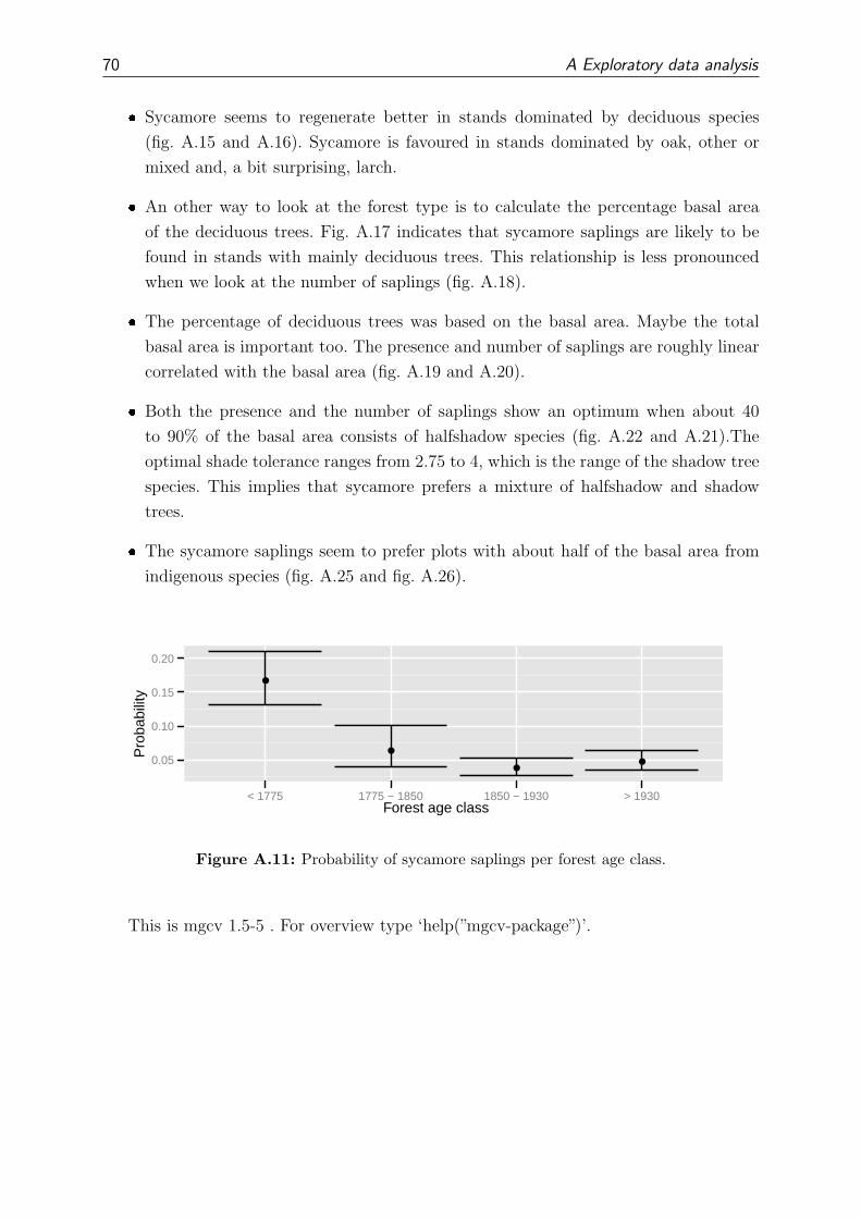
70 A Exploratory data analysis
� Sycamore seems to regenerate better in stands dominated by deciduous species
(fig. A.15 and A.16). Sycamore is favoured in stands dominated by oak, other or
mixed and, a bit surprising, larch.
� An other way to look at the forest type is to calculate the percentage basal area
of the deciduous trees. Fig. A.17 indicates that sycamore saplings are likely to be
found in stands with mainly deciduous trees. This relationship is less pronounced
when we look at the number of saplings (fig. A.18).
� The percentage of deciduous trees was based on the basal area. Maybe the total
basal area is important too. The presence and number of saplings are roughly linear
correlated with the basal area (fig. A.19 and A.20).
� Both the presence and the number of saplings show an optimum when about 40
to 90% of the basal area consists of halfshadow species (fig. A.22 and A.21).The
optimal shade tolerance ranges from 2.75 to 4, which is the range of the shadow tree
species. This implies that sycamore prefers a mixture of halfshadow and shadow
trees.
� The sycamore saplings seem to prefer plots with about half of the basal area from
indigenous species (fig. A.25 and fig. A.26).
Forest age class
Pro
babi
lity
0.05
0.10
0.15
0.20
●
●
●●
< 1775 1775 − 1850 1850 − 1930 > 1930
Figure A.11: Probability of sycamore saplings per forest age class.
This is mgcv 1.5-5 . For overview type ‘help(”mgcv-package”)’.

A.4 Forest management 71
Forest age classLog1
0 nu
mbe
r of
sap
lings
0.02
0.04
0.06
0.08
0.10
0.12
0.14
●
●
● ●
< 1775 1775 − 1850 1850 − 1930 > 1930
Figure A.12: Average number of sycamore saplings in a plot per forest age class.
Stand age class
Pro
babi
lity
0.04
0.06
0.08
0.10
0.12
●
●
●
●
Young Medium Old Mixed
Figure A.13: Probability of sycamore saplings per stand age class.
Stand age classLog1
0 nu
mbe
r of
sap
lings
0.02
0.04
0.06
0.08
●
●
●
●
Young Medium Old Mixed
Figure A.14: Average number of sycamore saplings in a plot per stand age class.

72 A Exploratory data analysis
Dominant tree species
Pro
babi
lity
0.05
0.10
0.15
0.20
0.25
●
● ●
●●
●
●
●●
Bee
ch
Bla
ck p
ine
Dou
glas
Larc
h
Oak
Oth
er o
f mix
ture
Pop
lar
Sco
tch
pine
Spr
uce
Figure A.15: Probability of sycamore saplings per dominant tree species.
Dominant tree species
Log1
0 nu
mbe
r of
sap
lings
−0.05
0.00
0.05
0.10
0.15
●
● ●
● ●
●●
● ●
Bee
ch
Bla
ck p
ine
Dou
glas
Larc
h
Oak
Oth
er o
f mix
ture
Pop
lar
Sco
tch
pine
Spr
uce
Figure A.16: Average number of sycamore saplings in a plot per dominant tree species.
Deciduous
Pre
senc
e
0.0
0.2
0.4
0.6
0.8
1.0
●●● ●●● ●●●●●●● ● ●●●● ●●●●● ●●● ●●● ●●● ●●● ● ●● ●●● ●●●● ●● ● ●● ●●● ●●● ●● ●● ●● ●●● ●● ●●● ● ●● ●●●●● ●● ●●● ●●● ●●● ●● ●●● ●● ● ●● ●●● ● ●● ● ●● ●●● ●● ● ●● ● ●●● ●● ●●● ●●●● ●● ● ●●●●● ●●● ●● ●● ● ●●● ●●● ●● ●● ● ●● ● ●●●● ●●● ●● ●● ●●●● ●● ●● ●● ●● ● ●●● ●●●● ●● ●●●● ●● ●●●●●● ●●● ●●●●● ●●● ●● ●● ● ● ●●●● ●● ●●● ●●● ●● ●●●● ●● ●● ●●●● ● ●●●●●●● ● ● ●●● ● ●● ●● ●●● ●● ● ●●●● ●●●●● ●●●● ● ● ●●● ●●●●●●●●●●●●● ●●●● ●●●●●●●● ●● ●●●● ●●● ● ●● ●●●● ●● ●● ● ●●●●●●●● ●● ● ●● ●● ●● ●●● ● ●● ● ●● ●●● ●●●● ●●●● ●●●● ●● ●● ●● ●● ●●● ●●●● ●●●● ● ●● ●●●●● ●● ●●● ●● ●● ● ●●●● ●● ●●●●●●●● ●● ●● ●● ●●●● ●●● ●● ● ●●●● ● ●● ●●●●●●● ●●● ● ●●●●●● ●● ●●●● ●●● ●●● ●● ●●●●● ●●● ●●● ●●● ●●● ●●●● ●●●●●●●●● ●●●●●●●●●●●●●●●●● ●● ●●● ●●●● ●● ● ● ●● ●●●● ●●● ●● ●● ●● ●● ● ●●●● ●● ●●● ●● ●● ●●● ●●●●● ●●●●● ●●● ●● ●● ●●● ●●●●●●●● ● ●●●● ●● ●● ●●●● ●●●● ●●● ●●●● ●●● ●● ●● ●●● ● ●●●● ●● ● ●● ●●● ● ●●●●● ●● ●● ●● ● ●● ●● ●● ● ●● ● ●● ●● ●● ●●● ●● ●●●● ●● ●●●● ●●● ●● ●●●●●●●●● ●●●●●●● ●●●●●● ●●● ●●● ●● ●●●● ● ●● ●● ●●●●● ● ● ●● ●●●●●●●● ●●● ● ●●●●● ● ●● ●●●●●●●● ● ●● ● ●●● ● ●● ●● ●●●●● ●●● ●●●●● ●● ● ●●●● ●● ●●●●● ● ●●●● ● ●● ●●●●● ● ●● ●● ●●● ●● ●●●●● ●● ● ●●●● ●● ● ● ●●●●● ●●● ●● ●● ●● ●●●●● ●●●● ●● ●●● ●●● ●●●●● ●●● ● ●●● ●●●● ●●●● ●● ●●● ● ●● ●● ● ●●● ●● ●●● ●● ●●●●● ●●●●● ●●● ●●●● ●●●●●● ●●● ● ●● ●● ● ●●●● ●● ●●● ●●●●● ●● ● ●●●●●●●●● ●●●●●●●●● ● ●●● ● ●●●●●●●●● ●●●● ●●● ●● ●●●●●●●●●●●● ●●●●●●●●● ●●●● ● ●●●● ●●● ●●●●●●●●●●●●●●●●● ●●●●●●●●●●●●●●● ●●● ●●●●●●●●● ●●●●●●●●●● ●●● ● ●● ●●●●●●● ●●●● ●●● ●●●●● ●● ●● ●●● ●● ●●●● ●● ●●●●● ●● ●●●●●● ●●● ●● ●● ●●●● ●●●●●●●●●● ● ●●●●●●●●●●●●● ●●●●●● ●●●●● ●●●●●● ●●●● ●●●●●●● ●●●●●●●●●●●● ●●●●● ●●●●●●● ●●●● ●●●●● ●●● ●● ●●● ●● ●●● ●● ●● ●● ●●●● ●● ● ●● ● ●● ● ●● ●●● ● ●●● ● ●● ●●● ●● ●● ●● ●● ●●●● ●● ● ●●● ●●● ●● ●● ● ●●● ●●●●● ●●●●●● ● ● ●● ●●●●●● ● ●● ●● ●●●●● ●● ●●● ●● ●●●●●●●●● ● ●● ●● ●● ● ●●● ● ●● ●●●●●● ●●● ●● ●● ●●● ●● ● ●● ●● ●●●●● ●● ●●●● ●●●● ●●● ●●● ●●● ●●● ● ● ● ● ●●●● ●●● ●●● ●● ●● ●● ●● ●●●●●● ● ● ●● ●● ●● ●● ● ●●● ● ● ●● ●●● ●●●● ●● ●● ● ●● ●●● ●● ●● ● ●● ● ● ●● ●● ●●● ● ●● ●●● ● ●●●● ●● ●● ●● ● ●●●● ● ● ● ●● ● ●● ●● ● ●●● ●●● ●●● ●● ● ●●●●● ●● ●●● ● ●● ● ● ●●● ● ●● ●● ●●●● ●●● ●● ●●●●● ●● ●●● ● ●● ● ● ●●●●●●● ●●●●●●●●● ●●●●●●●●●●●●●●● ●●● ●●●●●● ●●● ●● ●●●●●●●●●●●●●●●●●● ●●●●●●●●●●● ●●● ●● ●●●● ●● ●●● ●●●●●●●●●●● ●●●●●●●●●●●● ●●●●●●●●●●● ●● ●●●●●●●● ●●●● ●●● ●●● ●● ●●●●●●●● ●●●● ●●●●●●●● ●●●●●●●●●●●● ●● ●●●●●● ●● ●● ●● ●●●●●●●●●●●●● ●●●●●●●●●●●●●●●●●●● ●●●● ●● ● ●● ●●●● ●●● ●●● ●●●●●●●●●●● ●●●●●●● ●●●●●●● ●●●●●●●●●●●● ●●●● ●●●●●●●●●●●●●●●●●● ●●●● ●●● ●●● ●●●●●●●●●● ●● ●● ●●● ●● ●●●●●● ●●●● ●● ●●●● ●●● ●●●●●● ●● ●●●●●●● ●●●●●●●●●● ●●● ● ●●●●●●● ●● ● ●● ●●●● ●●● ●● ●● ● ●●●●●●●●●● ●●●●● ● ● ●● ●●●● ●● ●● ●●● ●● ● ●● ●●● ● ●●●●●●● ●● ● ● ●●●● ●●● ●● ●● ● ●●●● ●●● ● ●● ●● ●●● ●●●● ●● ●● ●●●● ●● ●●●●● ● ●●● ●●●●●●●●●●●● ●● ●● ● ● ● ●● ● ●● ●●● ●● ● ●● ●● ●●●● ●● ● ●●● ●● ●●● ● ●●●●●● ● ● ●●●●●●●●●● ●●●● ● ●●●●●● ●● ●● ●●●●●●●●●●●●●●● ●● ●● ●●●●●●●● ●● ●●● ●● ●● ●●● ●●●● ●●
● ●● ●●●● ●●● ●●●●●●●●●●●●●● ●● ●●●●●●● ●● ●●●● ●● ●●●●●●●●●●● ●●●●●●●●●●●●●●●●●●●● ●●●●●● ● ●●●●● ●● ●●●●● ●●●● ●●●●●●●●●●● ● ●●●●● ●●● ●●●●●●●● ●●●●●●●●● ●●●● ●● ●●●●● ●●●● ●●● ●
0.0 0.2 0.4 0.6 0.8 1.0
Figure A.17: The presence of sycamore saplings by percentage deciduous basal area.

A.4 Forest management 73
DeciduousLog1
0 nu
mbe
r of
sap
lings
0.0
0.5
1.0
1.5
●●● ●●● ●●●●●●● ● ●●●● ●●●●● ●●● ●●● ●●● ●●● ● ●● ●●● ●●●● ●● ● ●● ●●● ●●● ●● ●● ●● ●●● ●● ●●● ● ●● ●●●●● ●● ●●● ●●● ●●● ●● ●●● ●● ● ●● ●●● ● ●● ● ●● ●●● ●● ● ●● ● ●●● ●● ●●● ●●●● ●● ● ●●●●● ●●● ●● ●● ● ●●● ●●● ●● ●● ● ●● ● ●●●● ●●● ●● ●● ●●●● ●● ●● ●● ●● ● ●●● ●●●● ●● ●●●● ●● ●●●●●● ●●● ●●●●● ●●● ●● ●● ● ● ●●●● ●● ●●● ●●● ●● ●●●● ●● ●● ●●●● ● ●●●●●●● ● ● ●●● ● ●● ●● ●●● ●● ● ●●●● ●●●●● ●●●● ● ● ●●● ●●●●●●●●●●●●● ●●●● ●●●●●●●● ●● ●●●● ●●● ● ●● ●●●● ●● ●● ● ●●●●●●●● ●● ● ●● ●● ●● ●●● ● ●● ● ●● ●●● ●●●● ●●●● ●●●● ●● ●● ●● ●● ●●● ●●●● ●●●● ● ●● ●●●●● ●● ●●● ●● ●● ● ●●●● ●● ●●●●●●●● ●● ●● ●● ●●●● ●●● ●● ● ●●●● ● ●● ●●●●●●● ●●● ● ●●●●●● ●● ●●●● ●●● ●●● ●● ●●●●● ●●● ●●● ●●● ●●● ●●●● ●●●●●●●●● ●●●●●●●●●●●●●●●●● ●● ●●● ●●●● ●● ● ● ●● ●●●● ●●● ●● ●● ●● ●● ● ●●●● ●● ●●● ●● ●● ●●● ●●●●● ●●●●● ●●● ●● ●● ●●● ●●●●●●●● ● ●●●● ●● ●● ●●●● ●●●● ●●● ●●●● ●●● ●● ●● ●●● ● ●●●● ●● ● ●● ●●● ● ●●●●● ●● ●● ●● ● ●● ●● ●● ● ●● ● ●● ●● ●● ●●● ●● ●●●● ●● ●●●● ●●● ●● ●●●●●●●●● ●●●●●●● ●●●●●● ●●● ●●● ●● ●●●● ● ●● ●● ●●●●● ● ● ●● ●●●●●●●● ●●● ● ●●●●● ● ●● ●●●●●●●● ● ●● ● ●●● ● ●● ●● ●●●●● ●●● ●●●●● ●● ● ●●●● ●● ●●●●● ● ●●●● ● ●● ●●●●● ● ●● ●● ●●● ●● ●●●●● ●● ● ●●●● ●● ● ● ●●●●● ●●● ●● ●● ●● ●●●●● ●●●● ●● ●●● ●●● ●●●●● ●●● ● ●●● ●●●● ●●●● ●● ●●● ● ●● ●● ● ●●● ●● ●●● ●● ●●●●● ●●●●● ●●● ●●●● ●●●●●● ●●● ● ●● ●● ● ●●●● ●● ●●● ●●●●● ●● ● ●●●●●●●●● ●●●●●●●●● ● ●●● ● ●●●●●●●●● ●●●● ●●● ●● ●●●●●●●●●●●● ●●●●●●●●● ●●●● ● ●●●● ●●● ●●●●●●●●●●●●●●●●● ●●●●●●●●●●●●●●● ●●● ●●●●●●●●● ●●●●●●●●●● ●●● ● ●● ●●●●●●● ●●●● ●●● ●●●●● ●● ●● ●●● ●● ●●●● ●● ●●●●● ●● ●●●●●● ●●● ●● ●● ●●●● ●●●●●●●●●● ● ●●●●●●●●●●●●● ●●●●●● ●●●●● ●●●●●● ●●●● ●●●●●●● ●●●●●●●●●●●● ●●●●● ●●●●●●● ●●●● ●●●●● ●●● ●● ●●● ●● ●●● ●● ●● ●● ●●●● ●● ● ●● ● ●● ● ●● ●●● ● ●●● ● ●● ●●● ●● ●● ●● ●● ●●●● ●● ● ●●● ●●● ●● ●● ● ●●● ●●●●● ●●●●●● ● ● ●● ●●●●●● ● ●● ●● ●●●●● ●● ●●● ●● ●●●●●●●●● ● ●● ●● ●● ● ●●● ● ●● ●●●●●● ●●● ●● ●● ●●● ●● ● ●● ●● ●●●●● ●● ●●●● ●●●● ●●● ●●● ●●● ●●● ● ● ● ● ●●●● ●●● ●●● ●● ●● ●● ●● ●●●●●● ● ● ●● ●● ●● ●● ● ●●● ● ● ●● ●●● ●●●● ●● ●● ● ●● ●●● ●● ●● ● ●● ● ● ●● ●● ●●● ● ●● ●●● ● ●●●● ●● ●● ●● ● ●●●● ● ● ● ●● ● ●● ●● ● ●●● ●●● ●●● ●● ● ●●●●● ●● ●●● ● ●● ● ● ●●● ● ●● ●● ●●●● ●●● ●● ●●●●● ●● ●●● ● ●● ● ● ●●●●●●● ●●●●●●●●● ●●●●●●●●●●●●●●● ●●● ●●●●●● ●●● ●● ●●●●●●●●●●●●●●●●●● ●●●●●●●●●●● ●●● ●● ●●●● ●● ●●● ●●●●●●●●●●● ●●●●●●●●●●●● ●●●●●●●●●●● ●● ●●●●●●●● ●●●● ●●● ●●● ●● ●●●●●●●● ●●●● ●●●●●●●● ●●●●●●●●●●●● ●● ●●●●●● ●● ●● ●● ●●●●●●●●●●●●● ●●●●●●●●●●●●●●●●●●● ●●●● ●● ● ●● ●●●● ●●● ●●● ●●●●●●●●●●● ●●●●●●● ●●●●●●● ●●●●●●●●●●●● ●●●● ●●●●●●●●●●●●●●●●●● ●●●● ●●● ●●● ●●●●●●●●●● ●● ●● ●●● ●● ●●●●●● ●●●● ●● ●●●● ●●● ●●●●●● ●● ●●●●●●● ●●●●●●●●●● ●●● ● ●●●●●●● ●● ● ●● ●●●● ●●● ●● ●● ● ●●●●●●●●●● ●●●●● ● ● ●● ●●●● ●● ●● ●●● ●● ● ●● ●●● ● ●●●●●●● ●● ● ● ●●●● ●●● ●● ●● ● ●●●● ●●● ● ●● ●● ●●● ●●●● ●● ●● ●●●● ●● ●●●●● ● ●●● ●●●●●●●●●●●● ●● ●● ● ● ● ●● ● ●● ●●● ●● ● ●● ●● ●●●● ●● ● ●●● ●● ●●● ● ●●●●●● ● ● ●●●●●●●●●● ●●●● ● ●●●●●● ●● ●● ●●●●●●●●●●●●●●● ●● ●● ●●●●●●●● ●● ●●● ●● ●● ●●● ●●●● ●●
● ●● ●●●● ●●● ●●●●●●●●●●●●●● ●● ●●●●●
●● ●● ●●●● ●● ●●●●●●●●●●● ●●●●●
●●●●●●●●●●●●●●
● ●●●●●● ● ●●●●● ●● ●●●●● ●●●● ●●●●●●●●●●
● ● ●●●●●●●●●●●●●●●● ●●●●●●●●
● ●●●● ●● ●●
●
●● ●●●●●●
●●
0.0 0.2 0.4 0.6 0.8 1.0
Figure A.18: The log10 number of sycamore saplings by percentage deciduous basal area.
TotalBasalArea
Pre
senc
e
0.0
0.2
0.4
0.6
0.8
1.0
●●●● ● ●●●● ●●● ●● ●● ●●●● ●●● ● ●● ● ●● ●● ●● ●● ● ●●● ●● ●●●● ●● ● ●● ●● ●● ● ●●● ●● ● ●● ●●●●● ●●● ●● ●●● ● ● ●● ●●● ●● ●● ●●● ●● ● ●● ● ●●●●● ●● ●●● ●● ●● ● ●● ● ●● ● ●●●● ●●● ●● ●● ●● ●● ● ●● ●● ● ●●● ●● ● ●●● ●● ● ●● ●●●● ●● ●● ● ●● ● ● ●●● ● ●●●● ●● ●● ● ● ●● ●● ● ●● ●●● ●● ●●● ●●● ●● ●● ● ●●● ●●● ●● ●●● ●●● ●● ●● ●● ●● ● ●●● ● ● ●● ● ●●● ●●● ● ●● ●● ●●● ●● ●●● ●● ●●● ●● ● ●●● ●●● ● ● ●● ●● ●● ●● ● ●● ●● ●● ● ●●●● ●● ●● ●●●● ●● ●● ●● ● ● ●●● ● ●●●● ●● ●● ●● ● ● ●● ●● ●●●● ● ●●●● ● ●● ●● ●●● ●● ●● ●● ●●● ● ●● ● ● ●● ● ●●● ● ●● ●● ●●● ● ●● ●●● ●● ●● ● ●● ●● ● ●●● ●● ● ● ● ●●● ●●● ● ●● ●● ●●●●● ●● ●● ●●●● ● ●●● ●●●●● ●● ●● ● ● ●●●● ● ● ●● ●● ● ●● ●● ● ●●●● ●●● ●●● ● ●● ●● ● ● ●● ● ●●● ● ●● ●●● ●● ●● ● ●●●● ●● ● ●● ●● ● ●● ●●● ●●● ● ●● ● ●●● ●● ●● ●● ●● ●● ●●●● ●●● ● ● ●● ●●● ● ● ●● ●●●●● ●● ●● ●● ● ●● ●● ● ●● ● ●● ●●●●● ● ●● ●●● ●● ●● ●●● ●●● ●● ●● ●● ●● ●●● ●● ● ●●● ● ● ●● ● ●●● ●● ● ●●●●● ● ● ●● ● ●● ● ● ●● ●●● ● ●● ●● ●●● ●●●●● ● ●● ●● ●● ●●● ● ●● ● ●●● ●● ● ●●●●● ●● ● ●● ● ●● ● ●● ●●● ●● ● ●●● ● ● ●●● ●● ●● ● ●● ●● ●●●● ● ●●● ● ● ●● ●● ●●● ●● ●●● ● ●● ● ●● ● ●● ●● ●●● ●●● ● ● ● ●● ●●● ●● ● ●● ● ●●● ●● ●●● ● ●● ●●● ●●● ● ●● ●●● ●●●● ● ● ●● ● ●● ●● ● ●●● ● ● ●● ● ●● ●●● ●●● ● ● ●●● ●● ●●●●● ●● ●● ● ●● ●●●● ● ●● ●● ●●● ●●●● ●● ● ● ●●● ● ●●●● ●● ●●●● ●● ●● ●● ● ● ●●●●● ● ●● ● ●● ● ●● ●● ●●● ●● ● ● ●● ●● ● ●●●● ● ●● ● ●●● ●● ● ●● ●●● ●●●●● ●●● ●●● ●● ●●● ●● ●●●● ●● ● ●●●●● ●● ●● ● ●●● ●●● ● ●●● ●● ●●● ●● ● ●● ● ● ●● ●● ●●● ● ●● ●●● ●● ● ● ●●● ●● ●●●● ● ● ● ●●● ● ●●● ● ●● ●●●● ●● ● ●●● ●● ●● ●●●● ●● ●● ●● ●●● ● ●●● ●●● ● ● ●● ●●●●● ●●● ●● ●●● ●●● ●● ●● ●● ●●● ●●● ● ●● ●●● ● ●●● ● ● ●●● ●● ●●●● ●● ●● ●● ● ●●● ●●● ●●● ●● ●●●●● ●●● ● ● ●●● ●●● ● ●● ● ●●●● ● ●●● ●● ● ● ●● ●● ●● ● ●●● ● ●● ●● ●●●● ●●● ● ●● ●●● ●● ●● ●● ● ●● ● ●●● ●● ● ●●● ● ●● ●● ●●●● ● ● ●● ●●●● ●●●● ●●● ●●● ●●● ● ●●● ●● ●● ● ● ●● ● ●● ●●●●●● ● ●● ● ● ●●● ● ●● ●● ●● ● ●● ●●● ●● ●●●●● ●● ● ●●● ● ●● ● ●● ● ●● ●● ●●● ●●● ●●●● ●● ●● ●●●● ● ●●● ●●● ● ●● ●●● ●● ●●● ● ●● ●● ●● ●● ●● ●● ●●● ● ● ●●●●● ●● ●● ●●● ● ●●● ●● ●● ●●● ● ● ●● ● ●● ● ●● ●●● ●● ●● ●●● ● ● ● ●● ●● ●●● ●● ● ● ●● ●● ● ● ●● ● ●●●●● ● ●●● ●● ● ●● ●● ●● ●● ●●●● ●● ● ●●●● ●●● ●● ●●● ●● ●●●● ●●●●● ● ●● ●●●● ●●● ●● ●● ● ●● ●●● ● ● ●●● ● ●● ●● ● ●● ●● ● ● ●●● ●●● ●● ●● ● ● ●●● ●● ●● ●● ●● ●● ● ●●●● ●●● ●● ●● ●●●● ● ●● ●●● ● ●● ● ● ● ●● ●● ●● ●●● ●● ●●● ● ● ●●●● ●● ●● ● ●●● ●● ●● ●● ●● ●●● ● ●●●●● ●●●●● ●●● ●● ●● ●●● ●●● ● ●● ●● ● ●●● ●● ●● ●● ● ●●● ● ●●● ●● ● ●● ● ●● ●● ●● ●● ● ● ●●● ●● ● ●● ● ●● ●●● ●● ●●● ●● ●●● ●●● ● ●● ●● ●●● ●● ●●●● ●● ●●● ● ●●● ●● ● ●● ● ●● ●●●● ●●●●● ● ●● ● ●●● ●● ● ● ●●●●●● ● ●● ● ●●●●● ●● ● ●●●● ● ●● ●●● ●● ● ●● ● ●●● ●●● ● ● ●● ● ● ●●● ●● ●●●● ● ● ●●●● ●●● ●● ● ●● ● ●●● ●● ●●● ● ●● ●● ●● ●● ● ●●● ●● ●● ●● ●●● ●●● ●●● ●●● ●● ● ●● ●● ●● ●● ●●● ●● ●● ●● ● ● ● ●●●● ● ●● ● ●●● ● ●●● ●●● ●●● ●● ●●● ● ● ●●● ● ●● ●● ●● ●● ●●●● ● ●●● ●●● ● ●●● ● ●● ●●● ● ●● ● ●●● ●● ●● ●● ●● ●● ●● ●● ●●● ● ●● ● ●●●● ●●● ● ●●●● ●●● ● ●● ●● ●● ●● ●● ●● ●●● ●●●● ●● ●● ● ● ●● ● ●●●● ●●● ●● ● ● ●●●● ●● ● ●● ● ● ●●●●●● ●●● ●● ● ●● ● ● ●●● ●● ●● ● ●●● ● ●●●● ●● ●●● ● ● ●● ● ●● ●● ●●● ● ●● ●● ●●● ● ● ●● ●●●● ●● ●● ● ● ● ●● ●● ●● ●● ●●● ● ●●●● ●● ● ●● ●●●● ●●● ●●● ● ●●● ● ●● ●●●● ●●● ●● ●● ●●●● ● ● ●●● ●●● ●●●● ●● ●●● ●●● ●● ● ●●● ●● ●● ●● ●● ●● ●● ●● ● ●● ●● ● ● ●● ●●● ●●● ● ● ●●●● ●● ●● ●● ●● ● ●● ●● ●● ●● ●● ●●● ● ●● ●● ●● ● ●● ●●● ●
● ●● ● ● ●●●● ● ● ●● ●●●● ●● ●●● ● ●●● ●●●●● ● ●● ● ●●●● ●● ●● ●● ● ●● ● ● ●●●● ● ●● ● ●●● ●● ● ●● ●● ●● ● ● ●● ●● ●● ● ●●●●● ●● ● ●●● ●● ●●● ● ●●● ●●●●●● ●● ●●●●● ●● ● ●●● ●● ● ●● ● ●● ●●●● ●● ●● ●●● ● ● ●●● ●●● ●● ●●● ●
0 20 40 60 80 100 120
Figure A.19: The presence of sycamore saplings by basal area.
TotalBasalAreaLog1
0 nu
mbe
r of
sap
lings
0.0
0.5
1.0
1.5
●●●● ● ●●●● ●●● ●● ●● ●●●● ●●● ● ●● ● ●● ●● ●● ●● ● ●●● ●● ●●●● ●● ● ●● ●● ●● ● ●●● ●● ● ●● ●●●●● ●●● ●● ●●● ● ● ●● ●●● ●● ●● ●●● ●● ● ●● ● ●●●●● ●● ●●● ●● ●● ● ●● ● ●● ● ●●●● ●●● ●● ●● ●● ●● ● ●● ●● ● ●●● ●● ● ●●● ●● ● ●● ●●●● ●● ●● ● ●● ● ● ●●● ● ●●●● ●● ●● ● ● ●● ●● ● ●● ●●● ●● ●●● ●●● ●● ●● ● ●●● ●●● ●● ●●● ●●● ●● ●● ●● ●● ● ●●● ● ● ●● ● ●●● ●●● ● ●● ●● ●●● ●● ●●● ●● ●●● ●● ● ●●● ●●● ● ● ●● ●● ●● ●● ● ●● ●● ●● ● ●●●● ●● ●● ●●●● ●● ●● ●● ● ● ●●● ● ●●●● ●● ●● ●● ● ● ●● ●● ●●●● ● ●●●● ● ●● ●● ●●● ●● ●● ●● ●●● ● ●● ● ● ●● ● ●●● ● ●● ●● ●●● ● ●● ●●● ●● ●● ● ●● ●● ● ●●● ●● ● ● ● ●●● ●●● ● ●● ●● ●●●●● ●● ●● ●●●● ● ●●● ●●●●● ●● ●● ● ● ●●●● ● ● ●● ●● ● ●● ●● ● ●●●● ●●● ●●● ● ●● ●● ● ● ●● ● ●●● ● ●● ●●● ●● ●● ● ●●●● ●● ● ●● ●● ● ●● ●●● ●●● ● ●● ● ●●● ●● ●● ●● ●● ●● ●●●● ●●● ● ● ●● ●●● ● ● ●● ●●●●● ●● ●● ●● ● ●● ●● ● ●● ● ●● ●●●●● ● ●● ●●● ●● ●● ●●● ●●● ●● ●● ●● ●● ●●● ●● ● ●●● ● ● ●● ● ●●● ●● ● ●●●●● ● ● ●● ● ●● ● ● ●● ●●● ● ●● ●● ●●● ●●●●● ● ●● ●● ●● ●●● ● ●● ● ●●● ●● ● ●●●●● ●● ● ●● ● ●● ● ●● ●●● ●● ● ●●● ● ● ●●● ●● ●● ● ●● ●● ●●●● ● ●●● ● ● ●● ●● ●●● ●● ●●● ● ●● ● ●● ● ●● ●● ●●● ●●● ● ● ● ●● ●●● ●● ● ●● ● ●●● ●● ●●● ● ●● ●●● ●●● ● ●● ●●● ●●●● ● ● ●● ● ●● ●● ● ●●● ● ● ●● ● ●● ●●● ●●● ● ● ●●● ●● ●●●●● ●● ●● ● ●● ●●●● ● ●● ●● ●●● ●●●● ●● ● ● ●●● ● ●●●● ●● ●●●● ●● ●● ●● ● ● ●●●●● ● ●● ● ●● ● ●● ●● ●●● ●● ● ● ●● ●● ● ●●●● ● ●● ● ●●● ●● ● ●● ●●● ●●●●● ●●● ●●● ●● ●●● ●● ●●●● ●● ● ●●●●● ●● ●● ● ●●● ●●● ● ●●● ●● ●●● ●● ● ●● ● ● ●● ●● ●●● ● ●● ●●● ●● ● ● ●●● ●● ●●●● ● ● ● ●●● ● ●●● ● ●● ●●●● ●● ● ●●● ●● ●● ●●●● ●● ●● ●● ●●● ● ●●● ●●● ● ● ●● ●●●●● ●●● ●● ●●● ●●● ●● ●● ●● ●●● ●●● ● ●● ●●● ● ●●● ● ● ●●● ●● ●●●● ●● ●● ●● ● ●●● ●●● ●●● ●● ●●●●● ●●● ● ● ●●● ●●● ● ●● ● ●●●● ● ●●● ●● ● ● ●● ●● ●● ● ●●● ● ●● ●● ●●●● ●●● ● ●● ●●● ●● ●● ●● ● ●● ● ●●● ●● ● ●●● ● ●● ●● ●●●● ● ● ●● ●●●● ●●●● ●●● ●●● ●●● ● ●●● ●● ●● ● ● ●● ● ●● ●●●●●● ● ●● ● ● ●●● ● ●● ●● ●● ● ●● ●●● ●● ●●●●● ●● ● ●●● ● ●● ● ●● ● ●● ●● ●●● ●●● ●●●● ●● ●● ●●●● ● ●●● ●●● ● ●● ●●● ●● ●●● ● ●● ●● ●● ●● ●● ●● ●●● ● ● ●●●●● ●● ●● ●●● ● ●●● ●● ●● ●●● ● ● ●● ● ●● ● ●● ●●● ●● ●● ●●● ● ● ● ●● ●● ●●● ●● ● ● ●● ●● ● ● ●● ● ●●●●● ● ●●● ●● ● ●● ●● ●● ●● ●●●● ●● ● ●●●● ●●● ●● ●●● ●● ●●●● ●●●●● ● ●● ●●●● ●●● ●● ●● ● ●● ●●● ● ● ●●● ● ●● ●● ● ●● ●● ● ● ●●● ●●● ●● ●● ● ● ●●● ●● ●● ●● ●● ●● ● ●●●● ●●● ●● ●● ●●●● ● ●● ●●● ● ●● ● ● ● ●● ●● ●● ●●● ●● ●●● ● ● ●●●● ●● ●● ● ●●● ●● ●● ●● ●● ●●● ● ●●●●● ●●●●● ●●● ●● ●● ●●● ●●● ● ●● ●● ● ●●● ●● ●● ●● ● ●●● ● ●●● ●● ● ●● ● ●● ●● ●● ●● ● ● ●●● ●● ● ●● ● ●● ●●● ●● ●●● ●● ●●● ●●● ● ●● ●● ●●● ●● ●●●● ●● ●●● ● ●●● ●● ● ●● ● ●● ●●●● ●●●●● ● ●● ● ●●● ●● ● ● ●●●●●● ● ●● ● ●●●●● ●● ● ●●●● ● ●● ●●● ●● ● ●● ● ●●● ●●● ● ● ●● ● ● ●●● ●● ●●●● ● ● ●●●● ●●● ●● ● ●● ● ●●● ●● ●●● ● ●● ●● ●● ●● ● ●●● ●● ●● ●● ●●● ●●● ●●● ●●● ●● ● ●● ●● ●● ●● ●●● ●● ●● ●● ● ● ● ●●●● ● ●● ● ●●● ● ●●● ●●● ●●● ●● ●●● ● ● ●●● ● ●● ●● ●● ●● ●●●● ● ●●● ●●● ● ●●● ● ●● ●●● ● ●● ● ●●● ●● ●● ●● ●● ●● ●● ●● ●●● ● ●● ● ●●●● ●●● ● ●●●● ●●● ● ●● ●● ●● ●● ●● ●● ●●● ●●●● ●● ●● ● ● ●● ● ●●●● ●●● ●● ● ● ●●●● ●● ● ●● ● ● ●●●●●● ●●● ●● ● ●● ● ● ●●● ●● ●● ● ●●● ● ●●●● ●● ●●● ● ● ●● ● ●● ●● ●●● ● ●● ●● ●●● ● ● ●● ●●●● ●● ●● ● ● ● ●● ●● ●● ●● ●●● ● ●●●● ●● ● ●● ●●●● ●●● ●●● ● ●●● ● ●● ●●●● ●●● ●● ●● ●●●● ● ● ●●● ●●● ●●●● ●● ●●● ●●● ●● ● ●●● ●● ●● ●● ●● ●● ●● ●● ● ●● ●● ● ● ●● ●●● ●●● ● ● ●●●● ●● ●● ●● ●● ● ●● ●● ●● ●● ●● ●●● ● ●● ●● ●● ● ●● ●●● ●
● ●● ● ● ●●●● ● ● ●● ●●●● ●● ●●● ● ●●● ●●●●●
● ●● ● ●●●● ●● ●● ●● ● ●● ● ● ●●●● ● ●●
● ●●● ●● ● ●● ●● ●● ●
● ●● ●● ●● ● ●●●●● ●● ● ●●● ●●
●●● ● ●●● ●●●●●●
●● ●●●●●●● ●
●●
● ●● ●●● ● ●● ●●●● ●● ●● ●●● ● ● ●
●
● ●●● ●●●
●
●●
0 20 40 60 80 100 120
Figure A.20: The log10 number of sycamore saplings by basal area.

74 A Exploratory data analysis
Halfshadow
Pre
senc
e
0.0
0.2
0.4
0.6
0.8
1.0
●● ●●● ●● ●● ●●●● ● ● ●●● ●● ●●● ●●● ●● ●●●● ●●● ● ●● ●● ●●● ●●●● ● ●● ● ●●●●● ●●●● ● ●●●● ●● ●●● ● ●● ●● ●●● ●● ●●● ●●● ●● ●●● ● ●● ●● ● ●●●● ●● ● ●● ●● ●●●● ●●● ● ● ●●● ●● ●●● ●●●● ● ●●● ● ●●● ● ●● ●●●● ● ●●●●● ●● ●●● ●●● ●● ●●● ●● ●●● ●● ●●● ●●●●● ●●●●● ●●● ● ●● ●●● ●● ●● ●●● ●●● ●●● ●● ●● ● ●● ●● ●●● ● ●● ●●●●● ●●● ●● ●●● ●● ●●●● ●● ● ●●●● ●● ● ●● ●●●●● ● ● ●● ● ●●● ●●●●●● ●●●●●● ●●● ●●● ● ●●●● ●●● ●●●● ●●●● ●●●● ●●●● ●●●●●● ●● ●● ●●● ● ●●● ● ●● ●●●● ●● ●● ● ●●●● ● ●● ●●● ● ●●●● ●● ●●● ●● ●●●● ●● ● ●● ●●●●●● ● ●●● ●● ●● ●●●● ●●● ●●● ●●●●● ● ●● ●●● ●● ●● ●● ● ●● ●● ●● ●●● ●● ● ●● ●●●●● ●● ●● ●●●●●●●●●●●●● ●●●● ●●●● ●●● ●● ●● ●● ●● ● ●●● ●● ●●●● ●●● ●●● ●● ● ●●●● ●●●● ● ●● ●● ●●● ● ●●● ● ●●●●● ●●● ●● ●●● ●●●● ●●● ●●●●●● ● ●●●●● ●● ●● ●● ●● ● ●● ●●● ●●● ●● ●● ● ●● ●●●● ● ●● ●● ●● ●● ●●● ●●●●●● ●●●● ●●● ●●● ●●●● ●●● ● ●● ● ●● ●●●● ●● ●● ●●●● ●●●● ● ●● ●●●● ●● ●● ●● ● ●●● ● ● ●● ●●● ● ●● ●●● ● ● ●● ●● ● ●● ●●● ● ●● ●● ●● ● ●●● ● ●●● ●●●●●●● ●●●● ●●● ●●● ● ●● ●● ●●●●● ●●●● ●●● ●●●● ●● ● ●●● ● ●● ●●● ●● ● ●● ●● ●● ●● ●● ●●●● ● ●● ● ● ●●●● ●● ●●● ● ●●●● ●●●● ●● ●●●●●● ●● ● ● ●●●●● ●●● ●●● ●● ●● ●●● ●● ●●● ●●● ●● ● ●●●● ●●●●●● ●● ●● ●●● ●● ● ●● ●● ●●● ● ●●●● ●●●● ●●● ●● ●● ● ● ● ●●●● ● ●● ●● ●●●● ●●●●● ●● ● ●●●●● ●●●● ●●●●● ●● ●● ●● ●●●●●● ●●● ●● ●● ●● ●● ●● ● ●●● ● ●● ●● ● ●● ● ●●● ● ●●●● ● ●● ● ●●● ●●●●● ● ●●● ●●● ● ●● ● ●● ●●● ●●● ● ●● ●●●● ● ●●●●●●● ●● ● ●●●● ●●●● ● ●●● ● ●● ●●●● ● ●● ●● ●● ●●● ●● ●● ●●● ●●●● ●●● ●●● ●● ●● ●● ● ●●● ●● ●●● ● ● ●● ●●● ●● ●●● ●● ●● ●● ●● ●●● ● ● ●● ● ●●● ● ●● ●● ●●● ●● ●● ● ●●● ●● ●●● ●●● ●● ● ●●● ●● ●●●●●●● ●●●● ● ●● ● ●●●●● ● ●● ●● ● ●●●● ● ●●● ● ●● ●●● ●●●● ●●● ●● ●●● ●● ●● ●● ● ●●●● ●● ●●● ● ●● ●● ●● ●●●● ●●●● ●● ●●● ● ●● ●● ●● ●●●● ● ●●●● ● ● ●●●● ● ●● ●●●●● ●● ●●● ●●●● ●● ● ●●●●●● ●●●● ●●●● ● ●●● ●●● ●● ● ●● ● ●●●●● ● ●●● ● ●● ●●● ●● ● ●● ●● ●● ●●● ●●● ●●● ●●● ● ●● ●● ● ●● ●● ● ● ●●●● ●● ● ●● ● ● ● ●● ●●●● ●●●●● ●● ● ● ●● ●●●●●● ●●● ●● ●● ●●● ● ●● ●●●●● ● ● ●●●●●● ●●● ● ● ●●● ● ●●● ● ●●●● ●● ●● ●●● ●●● ● ● ●●● ● ● ●●● ●●● ● ●●●●● ●●● ● ●●● ●● ●●● ●●● ● ● ●● ● ●● ● ●●● ●●● ● ●●● ● ●●●● ● ●●●●● ●● ●● ●●●●● ● ●● ● ●● ●● ●●● ●● ● ●●●● ●● ●● ● ●● ●●●● ● ●● ● ●● ● ● ●●●● ●●● ●●● ●●● ●●●●● ● ●● ● ●● ● ●●● ●● ● ● ●●● ●● ● ●● ●●● ●● ● ●●●● ●● ● ●● ● ●●● ●● ●● ●● ● ● ●●● ● ●● ●● ● ●●● ●●● ●● ●●●● ●●● ●●● ●● ●●● ●● ● ●●● ●● ●● ●●●● ●● ●●● ●●● ●●● ●● ●●●● ●●● ●● ● ●●● ●●● ●● ● ●●● ●●●●● ● ●●● ●●●●● ●●● ●●● ●● ●●● ●●● ●● ● ●●● ●● ● ●●● ●●● ●● ●● ● ●● ●● ● ●● ● ●●● ●●● ●●● ●●●● ●● ● ●●● ●●●●● ●●●●●● ●●● ●●●● ●●● ● ●●● ●●● ● ● ● ● ●●●●●● ●● ● ●● ●● ● ● ● ●●●● ● ● ●● ●●●●● ●● ●●● ●● ●● ●● ●● ●● ●●● ● ●● ●●● ● ●●● ●● ● ●●● ●●● ●●●● ●● ● ● ●●● ●● ●● ● ● ●● ● ●●● ● ●●●● ●● ● ● ●● ●●● ●●● ●● ●● ●●● ●●●●●●● ●● ● ● ●● ●●●●● ●●●●●●●●●●●●● ●●●● ● ●● ● ●● ●● ●● ●●●●●●● ● ●●●●● ●● ●●● ●●● ● ●● ●●● ●● ●●●●● ●● ●● ● ●● ●● ●●●●●● ●● ● ●● ●● ●● ●●● ●●● ●●●● ●●● ●● ●● ●●●● ●● ●● ●●● ● ● ●●●●●●●● ● ●●● ●● ● ● ●●● ●● ●●● ●● ●● ●● ●● ●● ●● ● ● ●●●●●●● ●●● ● ●●●● ●● ●● ● ● ● ● ●●●● ● ●● ● ●●●● ● ●●● ●●● ● ●● ●●● ●●● ● ●● ● ●● ● ●●● ● ● ●●●● ●●●● ●● ● ●●● ● ●● ●● ● ●● ● ●● ● ●● ●● ● ● ●●● ●●● ● ● ●● ●● ● ●● ● ● ●● ● ●● ●● ●● ● ●●● ●●●● ●●● ● ●● ● ●● ●● ●● ●● ● ● ●● ●●● ●● ●● ● ●●● ●● ●●● ● ●● ●●● ●●●● ● ● ●●● ● ● ●● ●●● ● ● ●
● ●● ●● ●● ● ●● ●● ●● ●● ● ●● ●●● ●● ●● ●●● ●● ●●● ● ●● ●●● ● ●● ●● ● ●● ●● ● ●●● ● ●●● ●● ●●●●●● ● ● ● ● ●●● ● ●●●● ●● ●● ●● ●● ●● ●●●● ●●● ●● ●● ●● ●● ● ●● ●●● ● ●● ● ●● ● ●● ●●● ●● ● ● ●● ●● ●●● ● ●●● ●● ● ●●● ● ●● ●● ●●● ●
0.0 0.2 0.4 0.6 0.8 1.0
Figure A.21: The presence of sycamore saplings by percentage half shadow basal area.
HalfshadowLog1
0 nu
mbe
r of
sap
lings
0.0
0.5
1.0
1.5
●● ●●● ●● ●● ●●●● ● ● ●●● ●● ●●● ●●● ●● ●●●● ●●● ● ●● ●● ●●● ●●●● ● ●● ● ●●●●● ●●●● ● ●●●● ●● ●●● ● ●● ●● ●●● ●● ●●● ●●● ●● ●●● ● ●● ●● ● ●●●● ●● ● ●● ●● ●●●● ●●● ● ● ●●● ●● ●●● ●●●● ● ●●● ● ●●● ● ●● ●●●● ● ●●●●● ●● ●●● ●●● ●● ●●● ●● ●●● ●● ●●● ●●●●● ●●●●● ●●● ● ●● ●●● ●● ●● ●●● ●●● ●●● ●● ●● ● ●● ●● ●●● ● ●● ●●●●● ●●● ●● ●●● ●● ●●●● ●● ● ●●●● ●● ● ●● ●●●●● ● ● ●● ● ●●● ●●●●●● ●●●●●● ●●● ●●● ● ●●●● ●●● ●●●● ●●●● ●●●● ●●●● ●●●●●● ●● ●● ●●● ● ●●● ● ●● ●●●● ●● ●● ● ●●●● ● ●● ●●● ● ●●●● ●● ●●● ●● ●●●● ●● ● ●● ●●●●●● ● ●●● ●● ●● ●●●● ●●● ●●● ●●●●● ● ●● ●●● ●● ●● ●● ● ●● ●● ●● ●●● ●● ● ●● ●●●●● ●● ●● ●●●●●●●●●●●●● ●●●● ●●●● ●●● ●● ●● ●● ●● ● ●●● ●● ●●●● ●●● ●●● ●● ● ●●●● ●●●● ● ●● ●● ●●● ● ●●● ● ●●●●● ●●● ●● ●●● ●●●● ●●● ●●●●●● ● ●●●●● ●● ●● ●● ●● ● ●● ●●● ●●● ●● ●● ● ●● ●●●● ● ●● ●● ●● ●● ●●● ●●●●●● ●●●● ●●● ●●● ●●●● ●●● ● ●● ● ●● ●●●● ●● ●● ●●●● ●●●● ● ●● ●●●● ●● ●● ●● ● ●●● ● ● ●● ●●● ● ●● ●●● ● ● ●● ●● ● ●● ●●● ● ●● ●● ●● ● ●●● ● ●●● ●●●●●●● ●●●● ●●● ●●● ● ●● ●● ●●●●● ●●●● ●●● ●●●● ●● ● ●●● ● ●● ●●● ●● ● ●● ●● ●● ●● ●● ●●●● ● ●● ● ● ●●●● ●● ●●● ● ●●●● ●●●● ●● ●●●●●● ●● ● ● ●●●●● ●●● ●●● ●● ●● ●●● ●● ●●● ●●● ●● ● ●●●● ●●●●●● ●● ●● ●●● ●● ● ●● ●● ●●● ● ●●●● ●●●● ●●● ●● ●● ● ● ● ●●●● ● ●● ●● ●●●● ●●●●● ●● ● ●●●●● ●●●● ●●●●● ●● ●● ●● ●●●●●● ●●● ●● ●● ●● ●● ●● ● ●●● ● ●● ●● ● ●● ● ●●● ● ●●●● ● ●● ● ●●● ●●●●● ● ●●● ●●● ● ●● ● ●● ●●● ●●● ● ●● ●●●● ● ●●●●●●● ●● ● ●●●● ●●●● ● ●●● ● ●● ●●●● ● ●● ●● ●● ●●● ●● ●● ●●● ●●●● ●●● ●●● ●● ●● ●● ● ●●● ●● ●●● ● ● ●● ●●● ●● ●●● ●● ●● ●● ●● ●●● ● ● ●● ● ●●● ● ●● ●● ●●● ●● ●● ● ●●● ●● ●●● ●●● ●● ● ●●● ●● ●●●●●●● ●●●● ● ●● ● ●●●●● ● ●● ●● ● ●●●● ● ●●● ● ●● ●●● ●●●● ●●● ●● ●●● ●● ●● ●● ● ●●●● ●● ●●● ● ●● ●● ●● ●●●● ●●●● ●● ●●● ● ●● ●● ●● ●●●● ● ●●●● ● ● ●●●● ● ●● ●●●●● ●● ●●● ●●●● ●● ● ●●●●●● ●●●● ●●●● ● ●●● ●●● ●● ● ●● ● ●●●●● ● ●●● ● ●● ●●● ●● ● ●● ●● ●● ●●● ●●● ●●● ●●● ● ●● ●● ● ●● ●● ● ● ●●●● ●● ● ●● ● ● ● ●● ●●●● ●●●●● ●● ● ● ●● ●●●●●● ●●● ●● ●● ●●● ● ●● ●●●●● ● ● ●●●●●● ●●● ● ● ●●● ● ●●● ● ●●●● ●● ●● ●●● ●●● ● ● ●●● ● ● ●●● ●●● ● ●●●●● ●●● ● ●●● ●● ●●● ●●● ● ● ●● ● ●● ● ●●● ●●● ● ●●● ● ●●●● ● ●●●●● ●● ●● ●●●●● ● ●● ● ●● ●● ●●● ●● ● ●●●● ●● ●● ● ●● ●●●● ● ●● ● ●● ● ● ●●●● ●●● ●●● ●●● ●●●●● ● ●● ● ●● ● ●●● ●● ● ● ●●● ●● ● ●● ●●● ●● ● ●●●● ●● ● ●● ● ●●● ●● ●● ●● ● ● ●●● ● ●● ●● ● ●●● ●●● ●● ●●●● ●●● ●●● ●● ●●● ●● ● ●●● ●● ●● ●●●● ●● ●●● ●●● ●●● ●● ●●●● ●●● ●● ● ●●● ●●● ●● ● ●●● ●●●●● ● ●●● ●●●●● ●●● ●●● ●● ●●● ●●● ●● ● ●●● ●● ● ●●● ●●● ●● ●● ● ●● ●● ● ●● ● ●●● ●●● ●●● ●●●● ●● ● ●●● ●●●●● ●●●●●● ●●● ●●●● ●●● ● ●●● ●●● ● ● ● ● ●●●●●● ●● ● ●● ●● ● ● ● ●●●● ● ● ●● ●●●●● ●● ●●● ●● ●● ●● ●● ●● ●●● ● ●● ●●● ● ●●● ●● ● ●●● ●●● ●●●● ●● ● ● ●●● ●● ●● ● ● ●● ● ●●● ● ●●●● ●● ● ● ●● ●●● ●●● ●● ●● ●●● ●●●●●●● ●● ● ● ●● ●●●●● ●●●●●●●●●●●●● ●●●● ● ●● ● ●● ●● ●● ●●●●●●● ● ●●●●● ●● ●●● ●●● ● ●● ●●● ●● ●●●●● ●● ●● ● ●● ●● ●●●●●● ●● ● ●● ●● ●● ●●● ●●● ●●●● ●●● ●● ●● ●●●● ●● ●● ●●● ● ● ●●●●●●●● ● ●●● ●● ● ● ●●● ●● ●●● ●● ●● ●● ●● ●● ●● ● ● ●●●●●●● ●●● ● ●●●● ●● ●● ● ● ● ● ●●●● ● ●● ● ●●●● ● ●●● ●●● ● ●● ●●● ●●● ● ●● ● ●● ● ●●● ● ● ●●●● ●●●● ●● ● ●●● ● ●● ●● ● ●● ● ●● ● ●● ●● ● ● ●●● ●●● ● ● ●● ●● ● ●● ● ● ●● ● ●● ●● ●● ● ●●● ●●●● ●●● ● ●● ● ●● ●● ●● ●● ● ● ●● ●●● ●● ●● ● ●●● ●● ●●● ● ●● ●●● ●●●● ● ● ●●● ● ● ●● ●●● ● ● ●
● ●● ●● ●● ● ●● ●● ●● ●● ● ●● ●●● ●● ●● ●●● ●●
●●● ● ●● ●●● ● ●● ●● ● ●● ●● ● ●●● ● ●●
● ●● ●●●●●● ● ● ● ● ●
●● ● ●●●● ●● ●●●● ●● ●● ●●●●
●●● ●● ●● ●●●● ● ●
● ●●● ● ●●● ●●
●●
● ●●● ●● ● ● ●● ●● ●●● ● ●●● ●● ● ●●
● ● ●● ●●●
●
●●
0.0 0.2 0.4 0.6 0.8 1.0
Figure A.22: The log10 number of sycamore saplings by percentage halfshadow basal area.
ShadeTolerance
Pre
senc
e
0.0
0.2
0.4
0.6
0.8
1.0
●● ●●● ● ●●● ●●● ● ● ● ●●●●● ●●● ●●● ●● ●● ●● ●●● ● ●● ●● ●● ●●●●● ● ●● ●●● ●●● ●● ●● ● ● ● ●● ●● ●●● ● ●● ● ●●●● ●● ● ●● ●● ●● ●● ●● ● ●● ●● ● ●● ●● ●● ● ●● ●●●● ●● ●●●● ● ●●● ●● ●●● ● ●● ● ●● ● ●●●●● ●●● ●●●● ● ●●● ● ●●● ●●● ● ●● ●● ●●● ●● ●●● ●● ●●● ● ●● ●● ●● ●● ● ● ●● ●●● ●●● ● ●●● ●●● ●● ● ●● ● ●● ● ●●●● ●●● ●●● ●● ● ● ●● ● ● ●● ●● ●●● ● ●●●●● ●● ●● ● ●● ●● ● ●● ●●●●● ● ● ●● ● ● ● ●● ●●● ●● ●●●● ● ●●●● ● ●● ● ●●●● ●● ●●● ●●● ●●● ● ●●● ●●●● ●●●●●● ●● ●● ●● ● ● ●● ● ● ● ●●● ●● ●● ●●● ● ●●● ● ●● ●●● ●● ● ●● ●● ●●● ●● ● ● ● ●● ●● ●● ●● ●● ●● ●●● ● ●● ●● ●● ●● ●●● ● ●● ●●● ●● ● ●● ● ● ●●● ●● ●● ● ●● ● ●● ●●●● ●● ●●● ●●●● ● ●● ●● ● ●●●●●●●● ●● ●● ●●● ● ● ●●● ●●● ●● ● ●● ●●● ●●●● ●● ●● ●● ●●● ●●● ●● ●● ●●● ●●● ●●●●●● ●●● ●●●● ●●●●●● ●●● ●●● ●●●● ● ●● ●●● ●●●● ●● ●●●●● ●● ●● ●● ●● ●● ●●●● ● ●●● ●●● ●●● ●● ●● ●●●●● ●● ●● ● ●●● ● ●●● ●● ●● ● ●●● ●● ●● ●● ●●●● ● ●● ●●● ●●● ● ●● ●● ●●●● ●●●● ● ●● ●●●● ●● ● ●● ●● ●● ●● ●●● ●●● ● ●● ●●● ● ● ● ●● ●● ●● ●●● ● ● ●●● ● ●●●●● ● ●●● ●● ●● ●●● ●●●● ●● ●●●● ● ●● ●●●●●● ● ●● ●● ●● ●●●●● ●● ● ●●●● ●● ●●● ●● ● ●● ●● ●● ●● ●● ●●●● ● ●● ● ●●●● ●●● ●●● ●●●●● ●● ● ●●●●●● ●●● ●●● ● ● ●●● ● ●●● ●●● ●● ●● ● ●● ●●●●● ● ●● ●● ● ● ● ●● ●● ●●● ● ●● ●●●●● ●●● ●●●● ●●● ●● ●●● ●●●● ●●● ●● ●● ● ● ●● ●●● ● ●● ●● ●● ●● ● ●●● ● ●● ●●●●●● ● ● ●● ● ●●●●●● ●● ●● ●●● ●● ● ●●● ●● ●● ● ●●● ●●● ●● ● ●● ● ●● ●● ● ●● ●●●● ● ●● ●●● ●●●● ●●●●● ●●● ●● ●● ● ●● ●● ●●●● ● ●● ● ●●● ● ●● ●● ● ●● ● ● ●●● ● ●●●● ●● ●● ●● ●● ●●● ● ●● ●●●● ● ●● ●●●● ●● ● ●●●● ●● ● ●●●● ●●●●● ●●●● ●● ●● ● ●● ●● ● ●● ●●●● ● ●●● ●● ●● ●● ●●● ●● ●● ●● ●● ●● ●●● ●●● ● ● ●● ●●●●●●● ● ●● ●● ●●● ●● ●●●● ●● ●● ●● ●● ● ●●●● ●●● ● ●●●● ●● ●● ●● ●●● ●●● ● ●● ● ●● ●● ●●● ●● ●●● ●●●●● ●● ● ●● ●● ● ●● ●● ●●●● ● ●●● ●●● ●● ● ●●● ●●●● ● ●● ●● ●●● ● ● ● ●●● ● ●●● ●● ●●●● ● ●● ● ●● ● ●●● ●● ● ●●● ●● ●● ●●●●●● ● ●●● ● ●●● ●●● ●● ● ●● ●● ●● ●●● ●●●● ●●●● ● ●● ●●● ●● ● ●● ●●● ●●●● ● ●● ●●● ●● ● ● ●● ●● ● ● ●●●● ● ●●● ● ●● ● ●● ●● ●●● ●●● ●● ● ●●● ●● ● ● ●● ●●● ●●● ●● ●●● ●● ●●● ● ●● ● ●● ●● ● ● ●● ●● ●● ●●● ●● ● ●● ● ●● ● ● ●●●● ●● ●● ●● ●●●● ●●● ●● ● ●● ●● ●●● ●●● ●●● ●●● ●●●● ●● ●●● ●●● ●● ●● ● ●● ● ●● ●●●● ● ●●●● ●● ●● ●● ●●● ●● ●● ● ●● ●● ●● ●● ● ●●●● ●●● ●● ● ●●●● ●● ●● ● ●● ●●●●● ●● ● ●●● ● ●●●● ●●● ●●● ●●● ●●●●● ●●●● ●● ● ●●● ●● ● ● ●●● ●● ●●● ●●● ●●● ●●● ● ●● ● ●●● ●● ●●● ●● ● ●● ● ●●● ●●● ●● ● ●● ● ●●●●● ●●●● ● ●● ●●● ●● ●● ● ●● ●●●● ●● ● ●●● ● ●●● ● ● ●●● ●●● ●● ●●●● ●●●● ●● ●●●● ●● ●●● ●●● ●● ● ●● ●●● ●● ●●●●● ● ●● ● ●●● ● ● ●● ●●● ●● ●● ●● ●● ●●● ● ●● ● ●●●● ●●● ● ●●●● ●●●● ●●● ● ● ●●● ● ●● ●●● ●● ● ● ●●●● ●● ●●●● ●●● ●●● ●● ●●●● ●● ●● ●● ●●● ●●●●●●● ●●● ●● ●●● ●●●● ● ●● ●●● ●● ●● ●● ●● ● ●● ● ● ●●● ● ●● ●● ● ●● ●● ●● ●● ●● ●●● ● ●●●● ● ●●● ●● ● ●● ● ●● ●● ●● ●● ●●● ● ●● ●● ● ●● ●●●●● ● ● ●● ●●● ● ● ●●● ●●●●●●● ●●● ● ●●● ●●●● ●●●●●●●●●●●●●● ●●●● ● ●● ●● ●●●● ●●●●● ●● ●● ●● ● ●● ●● ● ●● ●●● ●● ●●● ●●●● ● ● ●● ● ●● ●● ● ●● ●● ●●● ●● ● ●●●● ● ●● ●●●● ●●● ●●●● ●● ●●● ●●●●● ●●● ● ●● ●● ● ●●●●●●●●● ● ●● ●● ● ● ●●● ● ●● ●●● ●● ●● ●● ●● ●● ● ●● ● ●●●●●●● ●● ● ● ●●●● ●●●● ● ● ●●● ● ●● ●● ●● ●●●● ● ●● ●●●● ● ● ● ● ● ●● ● ●●● ●● ●● ● ●●● ● ● ●●●● ●●●● ●● ● ●●● ● ●● ●● ●●● ● ●● ● ●● ●● ●●●●● ● ●● ● ● ●● ●● ●●● ● ● ●● ● ●● ● ●●● ● ● ●● ● ●● ● ● ●●● ●● ●●● ● ●● ●●● ●●● ●● ● ●●● ● ●●● ●● ●● ●● ●● ● ●● ●●●● ● ●●● ●● ●● ●●● ● ● ●● ●●
● ●● ● ●● ● ●● ● ●●● ●● ●● ● ●●● ● ● ●●● ● ●●● ●●● ●●● ●●● ●● ● ●●● ● ●● ● ●●● ●● ● ● ● ●● ●● ●● ●● ●●● ● ●● ● ●●● ●●● ● ●●●●● ●● ● ●● ● ● ●●●● ● ● ● ●●●● ●●●● ● ●● ●●● ●●● ● ● ●● ● ●●● ● ● ●●●●● ●● ●●● ●● ●●● ● ● ●● ●●● ●●● ●
1.0 1.5 2.0 2.5 3.0 3.5 4.0 4.5
Figure A.23: The presence of sycamore saplings by shade tolerance.

A.4 Forest management 75
ShadeToleranceLog1
0 nu
mbe
r of
sap
lings
0.0
0.5
1.0
1.5
●● ●●● ● ●●● ●●● ● ● ● ●●●●● ●●● ●●● ●● ●● ●● ●●● ● ●● ●● ●● ●●●●● ● ●● ●●● ●●● ●● ●● ● ● ● ●● ●● ●●● ● ●● ● ●●●● ●● ● ●● ●● ●● ●● ●● ● ●● ●● ● ●● ●● ●● ● ●● ●●●● ●● ●●●● ● ●●● ●● ●●● ● ●● ● ●● ● ●●●●● ●●● ●●●● ● ●●● ● ●●● ●●● ● ●● ●● ●●● ●● ●●● ●● ●●● ● ●● ●● ●● ●● ● ● ●● ●●● ●●● ● ●●● ●●● ●● ● ●● ● ●● ● ●●●● ●●● ●●● ●● ● ● ●● ● ● ●● ●● ●●● ● ●●●●● ●● ●● ● ●● ●● ● ●● ●●●●● ● ● ●● ● ● ● ●● ●●● ●● ●●●● ● ●●●● ● ●● ● ●●●● ●● ●●● ●●● ●●● ● ●●● ●●●● ●●●●●● ●● ●● ●● ● ● ●● ● ● ● ●●● ●● ●● ●●● ● ●●● ● ●● ●●● ●● ● ●● ●● ●●● ●● ● ● ● ●● ●● ●● ●● ●● ●● ●●● ● ●● ●● ●● ●● ●●● ● ●● ●●● ●● ● ●● ● ● ●●● ●● ●● ● ●● ● ●● ●●●● ●● ●●● ●●●● ● ●● ●● ● ●●●●●●●● ●● ●● ●●● ● ● ●●● ●●● ●● ● ●● ●●● ●●●● ●● ●● ●● ●●● ●●● ●● ●● ●●● ●●● ●●●●●● ●●● ●●●● ●●●●●● ●●● ●●● ●●●● ● ●● ●●● ●●●● ●● ●●●●● ●● ●● ●● ●● ●● ●●●● ● ●●● ●●● ●●● ●● ●● ●●●●● ●● ●● ● ●●● ● ●●● ●● ●● ● ●●● ●● ●● ●● ●●●● ● ●● ●●● ●●● ● ●● ●● ●●●● ●●●● ● ●● ●●●● ●● ● ●● ●● ●● ●● ●●● ●●● ● ●● ●●● ● ● ● ●● ●● ●● ●●● ● ● ●●● ● ●●●●● ● ●●● ●● ●● ●●● ●●●● ●● ●●●● ● ●● ●●●●●● ● ●● ●● ●● ●●●●● ●● ● ●●●● ●● ●●● ●● ● ●● ●● ●● ●● ●● ●●●● ● ●● ● ●●●● ●●● ●●● ●●●●● ●● ● ●●●●●● ●●● ●●● ● ● ●●● ● ●●● ●●● ●● ●● ● ●● ●●●●● ● ●● ●● ● ● ● ●● ●● ●●● ● ●● ●●●●● ●●● ●●●● ●●● ●● ●●● ●●●● ●●● ●● ●● ● ● ●● ●●● ● ●● ●● ●● ●● ● ●●● ● ●● ●●●●●● ● ● ●● ● ●●●●●● ●● ●● ●●● ●● ● ●●● ●● ●● ● ●●● ●●● ●● ● ●● ● ●● ●● ● ●● ●●●● ● ●● ●●● ●●●● ●●●●● ●●● ●● ●● ● ●● ●● ●●●● ● ●● ● ●●● ● ●● ●● ● ●● ● ● ●●● ● ●●●● ●● ●● ●● ●● ●●● ● ●● ●●●● ● ●● ●●●● ●● ● ●●●● ●● ● ●●●● ●●●●● ●●●● ●● ●● ● ●● ●● ● ●● ●●●● ● ●●● ●● ●● ●● ●●● ●● ●● ●● ●● ●● ●●● ●●● ● ● ●● ●●●●●●● ● ●● ●● ●●● ●● ●●●● ●● ●● ●● ●● ● ●●●● ●●● ● ●●●● ●● ●● ●● ●●● ●●● ● ●● ● ●● ●● ●●● ●● ●●● ●●●●● ●● ● ●● ●● ● ●● ●● ●●●● ● ●●● ●●● ●● ● ●●● ●●●● ● ●● ●● ●●● ● ● ● ●●● ● ●●● ●● ●●●● ● ●● ● ●● ● ●●● ●● ● ●●● ●● ●● ●●●●●● ● ●●● ● ●●● ●●● ●● ● ●● ●● ●● ●●● ●●●● ●●●● ● ●● ●●● ●● ● ●● ●●● ●●●● ● ●● ●●● ●● ● ● ●● ●● ● ● ●●●● ● ●●● ● ●● ● ●● ●● ●●● ●●● ●● ● ●●● ●● ● ● ●● ●●● ●●● ●● ●●● ●● ●●● ● ●● ● ●● ●● ● ● ●● ●● ●● ●●● ●● ● ●● ● ●● ● ● ●●●● ●● ●● ●● ●●●● ●●● ●● ● ●● ●● ●●● ●●● ●●● ●●● ●●●● ●● ●●● ●●● ●● ●● ● ●● ● ●● ●●●● ● ●●●● ●● ●● ●● ●●● ●● ●● ● ●● ●● ●● ●● ● ●●●● ●●● ●● ● ●●●● ●● ●● ● ●● ●●●●● ●● ● ●●● ● ●●●● ●●● ●●● ●●● ●●●●● ●●●● ●● ● ●●● ●● ● ● ●●● ●● ●●● ●●● ●●● ●●● ● ●● ● ●●● ●● ●●● ●● ● ●● ● ●●● ●●● ●● ● ●● ● ●●●●● ●●●● ● ●● ●●● ●● ●● ● ●● ●●●● ●● ● ●●● ● ●●● ● ● ●●● ●●● ●● ●●●● ●●●● ●● ●●●● ●● ●●● ●●● ●● ● ●● ●●● ●● ●●●●● ● ●● ● ●●● ● ● ●● ●●● ●● ●● ●● ●● ●●● ● ●● ● ●●●● ●●● ● ●●●● ●●●● ●●● ● ● ●●● ● ●● ●●● ●● ● ● ●●●● ●● ●●●● ●●● ●●● ●● ●●●● ●● ●● ●● ●●● ●●●●●●● ●●● ●● ●●● ●●●● ● ●● ●●● ●● ●● ●● ●● ● ●● ● ● ●●● ● ●● ●● ● ●● ●● ●● ●● ●● ●●● ● ●●●● ● ●●● ●● ● ●● ● ●● ●● ●● ●● ●●● ● ●● ●● ● ●● ●●●●● ● ● ●● ●●● ● ● ●●● ●●●●●●● ●●● ● ●●● ●●●● ●●●●●●●●●●●●●● ●●●● ● ●● ●● ●●●● ●●●●● ●● ●● ●● ● ●● ●● ● ●● ●●● ●● ●●● ●●●● ● ● ●● ● ●● ●● ● ●● ●● ●●● ●● ● ●●●● ● ●● ●●●● ●●● ●●●● ●● ●●● ●●●●● ●●● ● ●● ●● ● ●●●●●●●●● ● ●● ●● ● ● ●●● ● ●● ●●● ●● ●● ●● ●● ●● ● ●● ● ●●●●●●● ●● ● ● ●●●● ●●●● ● ● ●●● ● ●● ●● ●● ●●●● ● ●● ●●●● ● ● ● ● ● ●● ● ●●● ●● ●● ● ●●● ● ● ●●●● ●●●● ●● ● ●●● ● ●● ●● ●●● ● ●● ● ●● ●● ●●●●● ● ●● ● ● ●● ●● ●●● ● ● ●● ● ●● ● ●●● ● ● ●● ● ●● ● ● ●●● ●● ●●● ● ●● ●●● ●●● ●● ● ●●● ● ●●● ●● ●● ●● ●● ● ●● ●●●● ● ●●● ●● ●● ●●● ● ● ●● ●●
● ●● ● ●● ● ●● ● ●●● ●● ●● ● ●●● ● ● ●●● ● ●●● ●
●● ●●● ●●● ●● ● ●●● ● ●● ● ●●● ●● ● ● ●
●● ●● ●● ●● ●●● ● ●●
● ●●● ●●● ● ●●●●● ●● ● ●● ● ● ●
●●● ● ● ● ●●●● ●●●
● ● ●● ●●●●●●
●●
●● ● ●●● ● ● ●●●●● ●● ●●● ●● ●●●
●
● ●● ●●●●
●
●●
1.0 1.5 2.0 2.5 3.0 3.5 4.0 4.5
Figure A.24: The log10 number of sycamore saplings by shade tolerance.
Indigenous
Pre
senc
e
0.0
0.2
0.4
0.6
0.8
1.0
● ●● ●●● ●●●●●● ●● ●●●●●●●● ●●● ●● ●●● ●●●●●●● ●● ●● ●●● ●●● ●● ●●●● ● ● ●● ●● ●●● ●● ●●●● ●●●●● ● ●●● ●● ●● ●● ● ●● ●●●● ● ●● ● ●●●●● ● ●● ●●● ● ●●●● ●●● ●●● ●●●●● ●● ● ●● ●● ●●● ●●●● ●● ●● ●●● ● ●●● ●●●●● ●● ●●● ●●●●● ●● ● ●● ●●● ●● ● ●● ● ●●● ● ●● ●●● ● ● ●● ●●● ●● ●● ●●●● ●● ●● ●●● ●●●●● ●●●● ●●●● ●● ●●● ●●● ●● ●● ● ●●● ●●●● ●● ●● ● ● ●● ● ●● ●● ●●●●● ● ● ●●● ● ●● ●●● ●● ●● ●● ●●● ●●● ● ●●● ●●●● ●●●● ●●●● ●●●● ●● ● ●●●● ●●●●●● ●● ●●● ●●● ● ●● ●● ●● ●●●● ●●●●●● ●●● ●● ●●● ●● ● ●● ●● ●●● ●● ● ●● ●●● ●●●● ●● ●●● ●● ●● ●●● ● ●●●● ●● ●●●● ●●● ●●●●● ●●● ●●●●● ●● ●●● ● ●●●●● ●●● ●● ●●● ●●●● ● ●● ●●●●●●●● ●● ●● ●● ●●● ●●●●●● ●●●● ●● ● ●●●● ● ●●● ●● ●● ●● ●● ●● ● ● ● ●● ● ● ● ●●● ●● ●● ●●●●●● ●●●●● ● ●●● ●●● ● ●●● ● ●● ●●● ●● ●●●● ●●●●●● ●● ●●●●● ●● ●● ● ●● ● ●●● ●●●● ●●●● ● ●● ●● ●●● ● ●● ●●● ●● ●● ●● ●● ●● ●●●● ●● ● ●● ● ●●●● ●●● ●● ●● ●●●● ●● ●●●●●●● ●● ●● ● ●● ●●● ●● ●●● ●● ● ●● ●● ● ●●● ●● ● ●●● ● ●●● ●● ●● ●● ●●● ● ●● ● ● ● ●●●● ●●● ●●● ●●●● ●●●● ●●● ●● ●●●● ●● ● ●● ●● ●● ●● ●●● ●●●● ●●●● ●●● ●● ●●● ●●● ●● ●● ●●● ● ●●● ●●● ●●●●● ●●● ● ●● ●●●● ●● ●● ●●● ●●● ●● ●●● ● ●●● ●●● ● ●● ● ●● ● ●● ●● ●● ● ●● ●● ● ●● ● ●● ●●● ●● ●● ●●●● ●● ●● ●● ●●● ●●● ●●●● ●●●● ● ●●● ● ●●● ●● ● ●●●●● ●● ● ●● ●● ●● ●●● ● ● ● ●●● ●● ●●● ●● ●●● ●● ●● ● ●●●● ●● ●●●● ●● ●●●● ●●● ●● ●●●● ●● ●●●● ●●● ●● ●●● ● ●● ●● ● ● ●●●●● ●●●●● ●●● ●●● ●●● ● ●● ●● ● ●● ●● ●● ● ● ● ●● ●●● ● ●●● ●●● ● ● ● ●● ● ●● ● ●●● ●● ●●●● ●● ●● ●●●●●● ● ●● ● ● ●● ●● ● ●●●● ●● ● ●●●●●● ●● ●● ●●● ●● ●● ● ●● ●● ●●● ●●● ●● ●● ● ●● ●● ●● ●●● ● ●●●●● ●● ●● ●●● ●● ●●● ●● ●●●●●●● ●● ●●●● ● ●●● ●● ● ●● ●●●●● ●● ● ●●●● ●● ● ●● ● ●● ●●● ●●●● ●● ●●●● ●●●● ●●● ●● ●●●●● ●● ●●● ●● ●● ●● ●● ● ●●●● ●● ●●●● ●● ●● ● ●● ● ●●● ● ● ● ●● ●● ●● ●● ●● ● ● ●●●●● ●● ●●●● ● ● ● ●● ● ● ● ●● ●● ●●● ●●● ●● ●●●●●●● ● ●●● ● ●●●● ● ●● ● ●●● ●● ●●● ●●● ●● ● ●●● ●●●● ●● ● ● ● ●●● ●● ●● ●● ●● ● ●●● ●●● ●●●● ●● ●● ●●● ●●●● ●●●● ●●● ●●●● ●● ●●● ●● ●● ●●● ●●●● ●●●● ●●● ●●●●●● ●● ● ●● ●●●●● ●●●● ●●●● ● ●● ●●● ●●● ●●● ● ●●● ●●●● ●● ●●● ●● ● ●●●● ● ●●●● ● ● ●●●●●●● ● ●●● ●●● ● ●● ●● ●●●● ●●●● ●●● ● ●●●● ● ●●●● ● ●●● ●● ●●● ● ●● ●●● ● ●● ●●●●●● ●●● ●● ●● ● ●●●● ● ● ● ●●●● ● ●● ●● ●● ●●● ● ● ● ●●●● ● ●●● ●●● ●●● ●●●● ●●●●● ●●● ●● ● ● ●● ●●● ●● ●● ●●● ●● ●● ● ●●● ●●●● ●● ●●●● ●● ● ●● ●●● ●●● ●●●● ●● ●●●● ●● ● ●●●● ● ● ●●● ● ● ●● ● ●● ● ●● ●●● ●●● ●● ●● ●●●●●● ● ●● ● ●●● ●● ●●●● ●● ●● ● ●●●●●●●●●● ●●● ●● ●●●●●● ● ●●●● ●●● ● ●● ●●● ● ●●● ●●● ●● ●●●●●● ●●● ●●● ● ●●● ●●● ●●●●● ●●●● ● ●● ●● ●●●●●●●●●● ●●●● ●●●●●●●●●● ●●● ●●● ●● ●●●● ●●●●●● ●● ●●●●●●●●●● ●● ●●●●● ● ●● ●●● ●●● ● ●● ●●● ●●● ●● ●● ●● ●● ●● ●● ●●● ●●● ●●● ●● ●●● ● ● ●● ●● ●●●● ●● ●● ●●●● ● ●● ● ●● ●●●●● ●● ● ●● ●●●● ●● ●●● ●●● ●● ●● ●●●●●●●● ●●● ● ● ●●●●●● ●●●●●●●●●●●●●●●●● ● ●●● ●● ● ●●● ●●● ● ● ● ● ●●● ●●● ●● ●● ●●● ●● ●● ●●●● ●●●● ●●● ● ●● ●●● ●●●● ●●●●● ●●● ● ●●●●●● ● ●● ● ●● ●●●●● ●● ●●●● ●●● ●●●●● ●●●●●●●●●●●●●● ●● ● ●●● ●● ●● ●● ● ●●● ●●● ●● ●● ●● ●●●● ● ●●●●●● ● ●●● ● ● ●● ●●● ●● ● ● ●●● ●●●● ● ●● ●● ●●● ●●●● ●●● ● ●●●● ●● ●●●● ●●● ●●● ●●●● ●● ● ●●● ●●● ● ●● ●●●● ●● ●●● ●●● ●● ●●● ● ●●● ●● ●●● ●● ●●● ●●● ●●●● ●● ●● ●●● ● ●● ●● ●● ●●●● ●●● ●●● ●● ●● ● ●●● ●●●●●●●●● ● ● ●● ●● ●● ●●● ●●●● ● ●● ● ●●●●●●●● ● ●● ●●
●● ●● ●●●●● ●● ● ●● ●●● ●●●●●● ●●●● ● ●● ●●● ●●● ●●● ●● ● ●●● ●●● ● ●●● ● ●● ●●● ● ●●● ●●● ● ●●● ●●● ●●● ●● ●● ●●● ●● ●● ● ●● ●● ●●●● ● ●● ●● ●● ●●●● ● ●● ●●● ●● ●● ●●● ●●● ● ●● ●●● ●● ●● ● ●● ● ●●● ● ● ● ● ● ●●● ●●●●
0.0 0.2 0.4 0.6 0.8 1.0
Figure A.25: The presence of sycamore saplings by percentage indigenous basal area.
IndigenousLog1
0 nu
mbe
r of
sap
lings
0.0
0.5
1.0
1.5
● ●● ●●● ●●●●●● ●● ●●●●●●●● ●●● ●● ●●● ●●●●●●● ●● ●● ●●● ●●● ●● ●●●● ● ● ●● ●● ●●● ●● ●●●● ●●●●● ● ●●● ●● ●● ●● ● ●● ●●●● ● ●● ● ●●●●● ● ●● ●●● ● ●●●● ●●● ●●● ●●●●● ●● ● ●● ●● ●●● ●●●● ●● ●● ●●● ● ●●● ●●●●● ●● ●●● ●●●●● ●● ● ●● ●●● ●● ● ●● ● ●●● ● ●● ●●● ● ● ●● ●●● ●● ●● ●●●● ●● ●● ●●● ●●●●● ●●●● ●●●● ●● ●●● ●●● ●● ●● ● ●●● ●●●● ●● ●● ● ● ●● ● ●● ●● ●●●●● ● ● ●●● ● ●● ●●● ●● ●● ●● ●●● ●●● ● ●●● ●●●● ●●●● ●●●● ●●●● ●● ● ●●●● ●●●●●● ●● ●●● ●●● ● ●● ●● ●● ●●●● ●●●●●● ●●● ●● ●●● ●● ● ●● ●● ●●● ●● ● ●● ●●● ●●●● ●● ●●● ●● ●● ●●● ● ●●●● ●● ●●●● ●●● ●●●●● ●●● ●●●●● ●● ●●● ● ●●●●● ●●● ●● ●●● ●●●● ● ●● ●●●●●●●● ●● ●● ●● ●●● ●●●●●● ●●●● ●● ● ●●●● ● ●●● ●● ●● ●● ●● ●● ● ● ● ●● ● ● ● ●●● ●● ●● ●●●●●● ●●●●● ● ●●● ●●● ● ●●● ● ●● ●●● ●● ●●●● ●●●●●● ●● ●●●●● ●● ●● ● ●● ● ●●● ●●●● ●●●● ● ●● ●● ●●● ● ●● ●●● ●● ●● ●● ●● ●● ●●●● ●● ● ●● ● ●●●● ●●● ●● ●● ●●●● ●● ●●●●●●● ●● ●● ● ●● ●●● ●● ●●● ●● ● ●● ●● ● ●●● ●● ● ●●● ● ●●● ●● ●● ●● ●●● ● ●● ● ● ● ●●●● ●●● ●●● ●●●● ●●●● ●●● ●● ●●●● ●● ● ●● ●● ●● ●● ●●● ●●●● ●●●● ●●● ●● ●●● ●●● ●● ●● ●●● ● ●●● ●●● ●●●●● ●●● ● ●● ●●●● ●● ●● ●●● ●●● ●● ●●● ● ●●● ●●● ● ●● ● ●● ● ●● ●● ●● ● ●● ●● ● ●● ● ●● ●●● ●● ●● ●●●● ●● ●● ●● ●●● ●●● ●●●● ●●●● ● ●●● ● ●●● ●● ● ●●●●● ●● ● ●● ●● ●● ●●● ● ● ● ●●● ●● ●●● ●● ●●● ●● ●● ● ●●●● ●● ●●●● ●● ●●●● ●●● ●● ●●●● ●● ●●●● ●●● ●● ●●● ● ●● ●● ● ● ●●●●● ●●●●● ●●● ●●● ●●● ● ●● ●● ● ●● ●● ●● ● ● ● ●● ●●● ● ●●● ●●● ● ● ● ●● ● ●● ● ●●● ●● ●●●● ●● ●● ●●●●●● ● ●● ● ● ●● ●● ● ●●●● ●● ● ●●●●●● ●● ●● ●●● ●● ●● ● ●● ●● ●●● ●●● ●● ●● ● ●● ●● ●● ●●● ● ●●●●● ●● ●● ●●● ●● ●●● ●● ●●●●●●● ●● ●●●● ● ●●● ●● ● ●● ●●●●● ●● ● ●●●● ●● ● ●● ● ●● ●●● ●●●● ●● ●●●● ●●●● ●●● ●● ●●●●● ●● ●●● ●● ●● ●● ●● ● ●●●● ●● ●●●● ●● ●● ● ●● ● ●●● ● ● ● ●● ●● ●● ●● ●● ● ● ●●●●● ●● ●●●● ● ● ● ●● ● ● ● ●● ●● ●●● ●●● ●● ●●●●●●● ● ●●● ● ●●●● ● ●● ● ●●● ●● ●●● ●●● ●● ● ●●● ●●●● ●● ● ● ● ●●● ●● ●● ●● ●● ● ●●● ●●● ●●●● ●● ●● ●●● ●●●● ●●●● ●●● ●●●● ●● ●●● ●● ●● ●●● ●●●● ●●●● ●●● ●●●●●● ●● ● ●● ●●●●● ●●●● ●●●● ● ●● ●●● ●●● ●●● ● ●●● ●●●● ●● ●●● ●● ● ●●●● ● ●●●● ● ● ●●●●●●● ● ●●● ●●● ● ●● ●● ●●●● ●●●● ●●● ● ●●●● ● ●●●● ● ●●● ●● ●●● ● ●● ●●● ● ●● ●●●●●● ●●● ●● ●● ● ●●●● ● ● ● ●●●● ● ●● ●● ●● ●●● ● ● ● ●●●● ● ●●● ●●● ●●● ●●●● ●●●●● ●●● ●● ● ● ●● ●●● ●● ●● ●●● ●● ●● ● ●●● ●●●● ●● ●●●● ●● ● ●● ●●● ●●● ●●●● ●● ●●●● ●● ● ●●●● ● ● ●●● ● ● ●● ● ●● ● ●● ●●● ●●● ●● ●● ●●●●●● ● ●● ● ●●● ●● ●●●● ●● ●● ● ●●●●●●●●●● ●●● ●● ●●●●●● ● ●●●● ●●● ● ●● ●●● ● ●●● ●●● ●● ●●●●●● ●●● ●●● ● ●●● ●●● ●●●●● ●●●● ● ●● ●● ●●●●●●●●●● ●●●● ●●●●●●●●●● ●●● ●●● ●● ●●●● ●●●●●● ●● ●●●●●●●●●● ●● ●●●●● ● ●● ●●● ●●● ● ●● ●●● ●●● ●● ●● ●● ●● ●● ●● ●●● ●●● ●●● ●● ●●● ● ● ●● ●● ●●●● ●● ●● ●●●● ● ●● ● ●● ●●●●● ●● ● ●● ●●●● ●● ●●● ●●● ●● ●● ●●●●●●●● ●●● ● ● ●●●●●● ●●●●●●●●●●●●●●●●● ● ●●● ●● ● ●●● ●●● ● ● ● ● ●●● ●●● ●● ●● ●●● ●● ●● ●●●● ●●●● ●●● ● ●● ●●● ●●●● ●●●●● ●●● ● ●●●●●● ● ●● ● ●● ●●●●● ●● ●●●● ●●● ●●●●● ●●●●●●●●●●●●●● ●● ● ●●● ●● ●● ●● ● ●●● ●●● ●● ●● ●● ●●●● ● ●●●●●● ● ●●● ● ● ●● ●●● ●● ● ● ●●● ●●●● ● ●● ●● ●●● ●●●● ●●● ● ●●●● ●● ●●●● ●●● ●●● ●●●● ●● ● ●●● ●●● ● ●● ●●●● ●● ●●● ●●● ●● ●●● ● ●●● ●● ●●● ●● ●●● ●●● ●●●● ●● ●● ●●● ● ●● ●● ●● ●●●● ●●● ●●● ●● ●● ● ●●● ●●●●●●●●● ● ● ●● ●● ●● ●●● ●●●● ● ●● ● ●●●●●●●● ● ●● ●●
●● ●● ●●●●● ●● ● ●● ●●● ●●●●●● ●●●● ● ●● ●
●● ●●● ●●● ●● ● ●●● ●●● ● ●●● ● ●● ●●
● ● ●●● ●●● ● ●●● ●●
● ●●● ●● ●● ●●●●● ●● ● ●● ●● ●
●●● ● ●● ●● ●● ●●●
● ● ●● ●●●●● ●
●●
●● ●●● ● ●● ●●● ●● ●● ● ●● ● ●●● ●
●
● ● ● ●●●●
●
●●
0.0 0.2 0.4 0.6 0.8 1.0
Figure A.26: The log10 number of sycamore saplings by percentage indigenous basal area.

76 A Exploratory data analysis
A.5 Soil
Information on the soil properties is available as a digital soil map (Van Ranst and Sys,
2000). The soil map contains three variables: the soil region, the soil type and the soil
series. The soil regions are a similar division as the ecological regions. Since there are
more than 30 different soil types we focus on the soil series. De Keersmaeker et al. (2001a)
suggests ordinating the texture and drainage class according to table A.1 and A.2. Because
we had only few observations of the texture classes ”X” and ”U” we merged them with
resp. ”Z” and ”U”.
Table A.1: Ordination of soil texture classes (De Keersmaeker et al., 2001a).
Texture class X Z S P L / G A E U V
Score 1 2 3 4 5 6 7 8 9
Table A.2: Ordination of soil drainage classes (De Keersmaeker et al., 2001a).
Drainage class X a b c d e / h f / i g
Score 1 2 3 4 5 6 7 8
� Most of the information on the soil type is captured by the soil texture. Fig. A.27 and
A.28 indicate that sycamore saplings prefer P, L and A textures which are soils with
a fair amount of silt. They also have fairly large sand fraction. The combination of
silt and sand results in fertile and well drained soils. The more extreme soil textures
are avoided. E and U soils have a high clay fraction which is very fertile but is not
a well drained as the other soils. The Z and S textures drain very good (to good?)
but the lack in fertility.
� The sycamore saplings do not have a very pronounced relationship with the drainage.
According to fig. A.29, the saplings prefer most but not wet soils. We find a simular
pattern for the number of saplings (fig. A.30).

A.5 Soil 77
Aggregated soil texture
Pro
babi
lity
0.05
0.10
0.15
0.20
●
●
●
●
●
●
●
Z S P L A E U
Figure A.27: Probability of sycamore saplings per aggregated soil texture.
Aggregated soil textureLog1
0 nu
mbe
r of
sap
lings
−0.05
0.00
0.05
0.10
0.15
●
●
●● ●
●
●
Z S P L A E U
Figure A.28: Average number of sycamore saplings in a plot per aggregated soil texture.
Soil Drain
Pro
babi
lity
0.1
0.2
0.3
0.4
●
●●
●●
●
●●
●
●
●
2 2.5 3 3.5 4 4.5 5 6 6.5 7 8
Figure A.29: Probability of sycamore saplings per soil drainage class.

78 A Exploratory data analysis
Soil drainge classLog1
0 nu
mbe
r of
sap
lings
−0.10
−0.05
0.00
0.05
0.10
0.15
0.20
●
●
●
●
●
●
●●
●
●
●
2 2.5 3 3.5 4 4.5 5 6 6.5 7 8
Figure A.30: Average number of sycamore saplings in a plot per soil drainage class.

79
Appendix B
Overview of the models
B.1 Gaussian models
Table B.1: Estimate, standard deviance, t-value and p-value of the parameters of the Gaussiani.i.d. model
Estimate Std. Error t value Pr(>|t|)(Intercept) -0.0173 0.0099 -1.7397 0.0820
AggregatedTextureS 0.0094 0.0115 0.8113 0.4173
AggregatedTextureA 0.0820 0.0228 3.6008 0.0003
AggregatedTextureL 0.0192 0.0202 0.9544 0.3400
AggregatedTextureP 0.0411 0.0191 2.1558 0.0312
AggregatedTextureE 0.0110 0.0233 0.4731 0.6362
AggregatedTextureU -0.0567 0.0499 -1.1360 0.2561
DominantSpeciesOther of mixture 0.0355 0.0140 2.5379 0.0112
DominantSpeciesPoplar -0.0108 0.0186 -0.5801 0.5619
DominantSpeciesOak 0.0383 0.0162 2.3669 0.0180
DominantSpeciesBlack pine 0.0098 0.0188 0.5213 0.6022
DominantSpeciesBeech -0.0551 0.0279 -1.9733 0.0486
DominantSpeciesLarch 0.0764 0.0315 2.4252 0.0154
DominantSpeciesSpruce -0.0254 0.0355 -0.7163 0.4739
DominantSpeciesDouglas -0.0473 0.0498 -0.9498 0.3423
EcoRegionZuidoostelijke heuvel-
zone
0.0095 0.0206 0.4636 0.6430
EcoRegionPleistocene riviervalleien 0.0758 0.0166 4.5765 0.0000
EcoRegionZuidwestelijke heuvel-
zone
0.0411 0.0253 1.6226 0.1048
EcoRegionCuestas 0.1523 0.0184 8.2644 0.0000
EcoRegionMidden-Vlaamse over-
gangsgebieden
0.1222 0.0289 4.2291 0.0000
EcoRegionPolders en de getijden-
schelde
0.0563 0.0326 1.7268 0.0843
EcoRegionKrijt-leemgebieden 0.0352 0.0360 0.9796 0.3274
EcoRegionWestelijke interfluvia 0.3643 0.0389 9.3528 0.0000
EcoRegionKrijtgebieden 0.1298 0.0557 2.3315 0.0198
EcoRegionGrindrivieren -0.0068 0.1150 -0.0587 0.9532
IN1 0.3037 0.2678 1.1341 0.2569
IN2 -0.4111 0.2066 -1.9902 0.0467
SL1 -0.0096 0.2277 -0.0424 0.9662
SL2 0.4538 0.2110 2.1511 0.0316
ST1 0.5039 0.2844 1.7721 0.0765
StandAgeOld 0.0354 0.0102 3.4709 0.0005
StandAgeMixed -0.0024 0.0151 -0.1609 0.8721
StandAgeYoung 0.0003 0.0140 0.0206 0.9836
Correlation structure of class corSpher representing
range nugget
8281.3724279 0.5953236

80 B Overview of the models
Table B.2: Estimate, standard deviance, t-value and p-value of the parameters of the Gaussianautocovariates model
Estimate Std. Error t value Pr(>|t|)(Intercept) -0.0176 0.0098 -1.7970 0.0725
AggregatedTextureS 0.0056 0.0114 0.4896 0.6245
AggregatedTextureA 0.0665 0.0226 2.9384 0.0033
AggregatedTextureL 0.0173 0.0200 0.8661 0.3865
AggregatedTextureP 0.0374 0.0189 1.9831 0.0475
AggregatedTextureE 0.0094 0.0231 0.4085 0.6830
AggregatedTextureU -0.0517 0.0494 -1.0477 0.2949
DominantSpeciesOther of mixture 0.0359 0.0138 2.5947 0.0095
DominantSpeciesPoplar -0.0131 0.0184 -0.7125 0.4762
DominantSpeciesOak 0.0328 0.0160 2.0507 0.0404
DominantSpeciesBlack pine 0.0096 0.0186 0.5169 0.6053
DominantSpeciesBeech -0.0354 0.0278 -1.2747 0.2025
DominantSpeciesLarch 0.0624 0.0312 1.9984 0.0458
DominantSpeciesSpruce -0.0258 0.0351 -0.7355 0.4621
DominantSpeciesDouglas -0.0399 0.0492 -0.8112 0.4173
EcoRegionZuidoostelijke heuvel-
zone
-0.0081 0.0205 -0.3970 0.6914
EcoRegionPleistocene riviervalleien 0.0465 0.0169 2.7556 0.0059
EcoRegionZuidwestelijke heuvel-
zone
0.0121 0.0254 0.4766 0.6337
EcoRegionCuestas 0.0825 0.0206 3.9960 0.0001
EcoRegionMidden-Vlaamse over-
gangsgebieden
0.0784 0.0292 2.6853 0.0073
EcoRegionPolders en de getijden-
schelde
0.0191 0.0327 0.5859 0.5580
EcoRegionKrijt-leemgebieden 0.0084 0.0358 0.2354 0.8140
EcoRegionWestelijke interfluvia 0.2361 0.0424 5.5651 0.0000
EcoRegionKrijtgebieden 0.0570 0.0560 1.0176 0.3090
EcoRegionGrindrivieren -0.0054 0.1138 -0.0476 0.9621
IN1 0.2413 0.2651 0.9104 0.3627
IN2 -0.3573 0.2045 -1.7473 0.0807
SL1 0.0143 0.2253 0.0633 0.9496
SL2 0.4060 0.2088 1.9441 0.0520
ST1 0.3359 0.2823 1.1901 0.2341
StandAgeOld 0.0319 0.0101 3.1632 0.0016
StandAgeMixed -0.0046 0.0149 -0.3077 0.7583
StandAgeYoung -0.0012 0.0138 -0.0868 0.9308
GAC10 0.4194 0.0580 7.2301 0.0000
Distance
Sem
i−va
rianc
e
0.00
0.01
0.02
0.03
0.04
0.05
● ●●
●●
● ●● ●
● ● ● ● ● ● ● ●● ● ●
●● ● ●
● ● ●●
●● ● ●
● ● ●●
● ● ● ●
● ●●
●●
●●
● ●● ● ● ● ● ● ● ●
● ● ●
●● ● ●
● ● ●●
●● ● ●
● ● ●●
● ●● ●
● ●●
●●
●●
● ●● ● ● ● ● ● ● ●
● ● ●
●● ● ●
● ● ● ●●
● ● ●● ● ●
●
● ●● ●
● ●●
●●
●●
● ●
● ● ● ● ● ●● ●
● ● ●
●● ● ●
●● ●
●●
● ● ● ● ●●
●
● ● ● ●
● ●●
●●
● ●● ●
● ● ● ● ● ● ● ●● ● ●
●● ● ●
● ● ●●
●● ● ●
● ● ●●
● ● ● ●
0 20000 40000 60000 80000
Model
● Raw
● i.i.d.
● AC
● SAR
● GLS
Figure B.1: Empirical and fitted variograms for the residuals of the Gaussian models.

B.1 Gaussian models 81
Table B.3: Estimate, standard deviance, z-value and p-value of the parameters of the simulta-neous autoregressive model
Estimate Std. Error z value Pr(>|z|)(Intercept) -0.0155 0.0110 -1.4034 0.1605
AggregatedTextureS 0.0094 0.0119 0.7892 0.4300
AggregatedTextureA 0.0594 0.0239 2.4820 0.0131
AggregatedTextureL 0.0206 0.0207 0.9955 0.3195
AggregatedTextureP 0.0395 0.0194 2.0333 0.0420
AggregatedTextureE 0.0064 0.0236 0.2713 0.7862
AggregatedTextureU -0.0484 0.0493 -0.9810 0.3266
DominantSpeciesOther of mixture 0.0363 0.0139 2.6177 0.0089
DominantSpeciesPoplar -0.0153 0.0184 -0.8324 0.4052
DominantSpeciesOak 0.0303 0.0160 1.8954 0.0580
DominantSpeciesBlack pine 0.0107 0.0186 0.5731 0.5666
DominantSpeciesBeech -0.0414 0.0278 -1.4882 0.1367
DominantSpeciesLarch 0.0682 0.0311 2.1959 0.0281
DominantSpeciesSpruce -0.0282 0.0350 -0.8067 0.4198
DominantSpeciesDouglas -0.0248 0.0491 -0.5046 0.6139
EcoRegionZuidoostelijke heuvel-
zone
0.0227 0.0233 0.9726 0.3308
EcoRegionPleistocene riviervalleien 0.0936 0.0205 4.5691 0.0000
EcoRegionZuidwestelijke heuvel-
zone
0.0683 0.0298 2.2884 0.0221
EcoRegionCuestas 0.1264 0.0224 5.6483 0.0000
EcoRegionMidden-Vlaamse over-
gangsgebieden
0.1217 0.0324 3.7552 0.0002
EcoRegionPolders en de getijden-
schelde
0.0578 0.0370 1.5632 0.1180
EcoRegionKrijt-leemgebieden 0.0516 0.0415 1.2443 0.2134
EcoRegionWestelijke interfluvia 0.3566 0.0508 7.0137 0.0000
EcoRegionKrijtgebieden 0.1349 0.0720 1.8722 0.0612
EcoRegionGrindrivieren -0.0084 0.1134 -0.0739 0.9411
IN1 0.2813 0.2638 1.0662 0.2863
IN2 -0.3924 0.2039 -1.9241 0.0543
SL1 -0.0266 0.2331 -0.1141 0.9091
SL2 0.4457 0.2114 2.1082 0.0350
ST1 0.4353 0.2797 1.5564 0.1196
StandAgeOld 0.0349 0.0102 3.4385 0.0006
StandAgeMixed -0.0061 0.0149 -0.4097 0.6820
StandAgeYoung -0.0019 0.0138 -0.1401 0.8886
Distance
Sem
i−va
rianc
e
0
5
10
15
20
25
●
●
●
●
●
●●
●●
● ● ● ● ●●
● ● ●● ● ● ● ● ● ● ● ● ● ●
●
●
● ●●
● ●●
●
●●
0 20000 40000 60000 80000
Model
● CAR
Figure B.2: Empirical and fitted variograms for the residuals of the Gaussian CAR model.
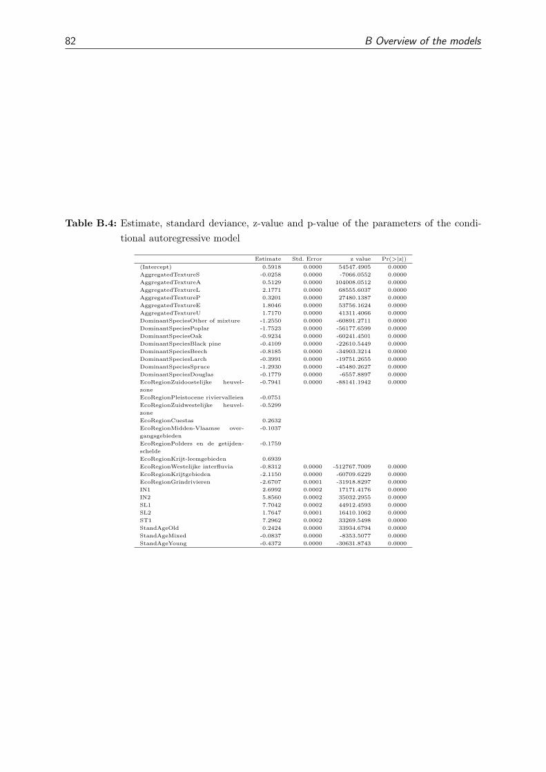
82 B Overview of the models
Table B.4: Estimate, standard deviance, z-value and p-value of the parameters of the condi-tional autoregressive model
Estimate Std. Error z value Pr(>|z|)(Intercept) 0.5918 0.0000 54547.4905 0.0000
AggregatedTextureS -0.0258 0.0000 -7066.0552 0.0000
AggregatedTextureA 0.5129 0.0000 104008.0512 0.0000
AggregatedTextureL 2.1771 0.0000 68555.6037 0.0000
AggregatedTextureP 0.3201 0.0000 27480.1387 0.0000
AggregatedTextureE 1.8046 0.0000 53756.1624 0.0000
AggregatedTextureU 1.7170 0.0000 41311.4066 0.0000
DominantSpeciesOther of mixture -1.2550 0.0000 -60891.2711 0.0000
DominantSpeciesPoplar -1.7523 0.0000 -56177.6599 0.0000
DominantSpeciesOak -0.9234 0.0000 -60241.4501 0.0000
DominantSpeciesBlack pine -0.4109 0.0000 -22610.5449 0.0000
DominantSpeciesBeech -0.8185 0.0000 -34903.3214 0.0000
DominantSpeciesLarch -0.3991 0.0000 -19751.2655 0.0000
DominantSpeciesSpruce -1.2930 0.0000 -45480.2627 0.0000
DominantSpeciesDouglas -0.1779 0.0000 -6557.8897 0.0000
EcoRegionZuidoostelijke heuvel-
zone
-0.7941 0.0000 -88141.1942 0.0000
EcoRegionPleistocene riviervalleien -0.0751
EcoRegionZuidwestelijke heuvel-
zone
-0.5299
EcoRegionCuestas 0.2632
EcoRegionMidden-Vlaamse over-
gangsgebieden
-0.1037
EcoRegionPolders en de getijden-
schelde
-0.1759
EcoRegionKrijt-leemgebieden 0.6939
EcoRegionWestelijke interfluvia -0.8312 0.0000 -512767.7009 0.0000
EcoRegionKrijtgebieden -2.1150 0.0000 -60709.6229 0.0000
EcoRegionGrindrivieren -2.6707 0.0001 -31918.8297 0.0000
IN1 2.6992 0.0002 17171.4176 0.0000
IN2 5.8560 0.0002 35032.2955 0.0000
SL1 7.7042 0.0002 44912.4593 0.0000
SL2 1.7647 0.0001 16410.1062 0.0000
ST1 7.2962 0.0002 33269.5498 0.0000
StandAgeOld 0.2424 0.0000 33934.6794 0.0000
StandAgeMixed -0.0837 0.0000 -8353.5077 0.0000
StandAgeYoung -0.4372 0.0000 -30631.8743 0.0000

B.1 Gaussian models 83
Table B.5: Estimate, standard deviance, t-value and p-value of the parameters of the gener-alised least squares model
Value Std.Error t-value p-value
(Intercept) -0.0130 0.0173 -0.7508 0.4529
AggregatedTextureS 0.0089 0.0132 0.6749 0.4998
AggregatedTextureA 0.0654 0.0265 2.4659 0.0137
AggregatedTextureL 0.0252 0.0217 1.1619 0.2454
AggregatedTextureP 0.0450 0.0205 2.1936 0.0284
AggregatedTextureE 0.0287 0.0245 1.1710 0.2417
AggregatedTextureU -0.0312 0.0492 -0.6339 0.5262
DominantSpeciesOther of mixture 0.0304 0.0135 2.2580 0.0240
DominantSpeciesPoplar -0.0219 0.0184 -1.1887 0.2347
DominantSpeciesOak 0.0341 0.0155 2.1956 0.0282
DominantSpeciesBlack pine 0.0167 0.0179 0.9287 0.3532
DominantSpeciesBeech -0.0043 0.0274 -0.1564 0.8757
DominantSpeciesLarch 0.0585 0.0299 1.9602 0.0501
DominantSpeciesSpruce -0.0354 0.0335 -1.0553 0.2914
DominantSpeciesDouglas -0.0126 0.0470 -0.2688 0.7881
EcoRegionZuidoostelijke heuvel-
zone
0.0238 0.0349 0.6801 0.4965
EcoRegionPleistocene riviervalleien 0.0840 0.0290 2.8954 0.0038
EcoRegionZuidwestelijke heuvel-
zone
0.0668 0.0388 1.7192 0.0857
EcoRegionCuestas 0.1381 0.0339 4.0726 0.0000
EcoRegionMidden-Vlaamse over-
gangsgebieden
0.1163 0.0455 2.5574 0.0106
EcoRegionPolders en de getijden-
schelde
0.0553 0.0546 1.0124 0.3114
EcoRegionKrijt-leemgebieden 0.0553 0.0527 1.0489 0.2943
EcoRegionWestelijke interfluvia 0.3470 0.0569 6.0953 0.0000
EcoRegionKrijtgebieden 0.1581 0.1041 1.5180 0.1291
EcoRegionGrindrivieren -0.0112 0.1253 -0.0891 0.9290
IN1 0.3086 0.2582 1.1950 0.2322
IN2 -0.4111 0.1987 -2.0696 0.0386
SL1 -0.0523 0.2483 -0.2107 0.8331
SL2 0.3764 0.2155 1.7464 0.0809
ST1 0.1778 0.2731 0.6511 0.5150
StandAgeOld 0.0316 0.0100 3.1637 0.0016
StandAgeMixed -0.0031 0.0145 -0.2145 0.8302
StandAgeYoung 0.0003 0.0134 0.0245 0.9805

84 B Overview of the models
B.2 Poisson models
Table B.6: Estimate, standard deviance, t-value and p-value of the parameters of the Poissoni.i.d. model
Estimate Std. Error z value Pr(>|z|)(Intercept) -6.6406 0.4723 -14.0609 0.0000
AggregatedTextureS 1.2300 0.1382 8.9023 0.0000
AggregatedTextureA 1.6181 0.1817 8.9054 0.0000
AggregatedTextureL 0.8435 0.1628 5.1812 0.0000
AggregatedTextureP 1.2524 0.1524 8.2182 0.0000
AggregatedTextureE 0.6119 0.1902 3.2179 0.0013
AggregatedTextureU -16.7805 907.5830 -0.0185 0.9852
DominantSpeciesOther of mixture 3.2590 0.4264 7.6434 0.0000
DominantSpeciesPoplar 2.2044 0.4345 5.0732 0.0000
DominantSpeciesOak 2.6069 0.4281 6.0900 0.0000
DominantSpeciesBlack pine -12.4286 203.8162 -0.0610 0.9514
DominantSpeciesBeech 1.5979 0.4663 3.4271 0.0006
DominantSpeciesLarch 3.1117 0.4497 6.9201 0.0000
DominantSpeciesSpruce -0.2923 0.8360 -0.3497 0.7266
DominantSpeciesDouglas -14.5073 710.2427 -0.0204 0.9837
DrainScore3 0.1068 0.1163 0.9188 0.3582
DrainScore6 -0.5598 0.0895 -6.2577 0.0000
DrainScore4 0.1136 0.1052 1.0806 0.2799
DrainScore7 -0.0897 0.1162 -0.7716 0.4404
DrainScore3.5 -1.1953 0.5941 -2.0119 0.0442
DrainScore4.5 -0.1508 0.1517 -0.9937 0.3204
DrainScore2 0.3927 0.3501 1.1217 0.2620
DrainScore8 -17.8862 1031.4317 -0.0173 0.9862
DrainScore6.5 -17.3893 929.6378 -0.0187 0.9851
DrainScore2.5 2.3719 0.5464 4.3410 0.0000
EcoRegionZuidoostelijke heuvel-
zone
2.9983 0.3462 8.6616 0.0000
EcoRegionPleistocene riviervalleien 3.3107 0.2853 11.6032 0.0000
EcoRegionZuidwestelijke heuvel-
zone
3.6299 0.3432 10.5754 0.0000
EcoRegionCuestas 3.6136 0.2626 13.7595 0.0000
EcoRegionMidden-Vlaamse over-
gangsgebieden
4.2918 0.3244 13.2303 0.0000
EcoRegionPolders en de getijden-
schelde
2.1469 0.3503 6.1281 0.0000
EcoRegionKrijt-leemgebieden 4.0292 0.5004 8.0522 0.0000
EcoRegionWestelijke interfluvia 6.0708 0.3602 16.8555 0.0000
EcoRegionKrijtgebieden 7.9409 0.9893 8.0269 0.0000
EcoRegionGrindrivieren -13.5816 3214.1828 -0.0042 0.9966
ForestAge> 1930 -0.3573 0.0852 -4.1961 0.0000
ForestAge< 1775 -0.0188 0.0856 -0.2199 0.8259
ForestAge1775 - 1850 -0.8088 0.1308 -6.1839 0.0000
IN1 -13.9077 1.9412 -7.1643 0.0000
ST1 11.2344 1.8843 5.9621 0.0000
StandAgeOld 1.2174 0.0818 14.8775 0.0000
StandAgeMixed 0.3295 0.1029 3.2031 0.0014
StandAgeYoung 0.5128 0.1021 5.0203 0.0000
TotalBasalArea -0.0168 0.0019 -8.7643 0.0000
XY0.1 37.1845 7.6124 4.8847 0.0000
XY0.2 -18.8631 5.2846 -3.5694 0.0004
XY0.3 -10.7388 3.4515 -3.1114 0.0019
XY1.0 -17.0732 6.3511 -2.6882 0.0072
XY1.1 -149.5557 297.0979 -0.5034 0.6147
XY1.2 -359.0530 201.4253 -1.7826 0.0747
XY2.0 -17.3762 4.0013 -4.3426 0.0000
XY2.1 415.0728 161.2692 2.5738 0.0101
XY3.0 -14.4818 2.0308 -7.1310 0.0000

B.2 Poisson models 85
Distance
Sem
i−va
rianc
e
0.0
0.5
1.0
1.5
2.0
2.5
3.0
3.5
● ●●
● ● ● ●● ● ● ● ● ● ● ● ● ●
● ● ●●
● ● ● ● ● ● ● ●● ● ●
● ● ●●
● ●● ●
● ●●
● ● ● ●● ● ● ● ● ● ● ● ● ●
● ● ●●
● ● ● ● ● ● ● ●● ● ●
● ● ●●
● ●● ●
● ●●
●
●● ● ●
●
● ● ● ● ● ● ●●
●●
●
●● ● ●
●
●●
●●
●●
●
●● ●
●
●● ●
●
0 20000 40000 60000 80000
Model
● Raw
● i.i.d.
● PAC
Figure B.3: Empirical and fitted variograms for the residuals of the Poisson models.

86 B Overview of the models
Table B.7: Estimate, standard deviance, t-value and p-value of the parameters of the Poissonautocovariates model
Estimate Std. Error z value Pr(>|z|)(Intercept) -6.6443 0.4726 -14.0587 0.0000
AggregatedTextureS 1.2315 0.1382 8.9129 0.0000
AggregatedTextureA 1.5785 0.1830 8.6257 0.0000
AggregatedTextureL 0.8280 0.1630 5.0785 0.0000
AggregatedTextureP 1.2617 0.1523 8.2864 0.0000
AggregatedTextureE 0.5966 0.1906 3.1304 0.0017
AggregatedTextureU -16.8164 923.0171 -0.0182 0.9855
DominantSpeciesOther of mixture 3.2612 0.4266 7.6445 0.0000
DominantSpeciesPoplar 2.1982 0.4349 5.0547 0.0000
DominantSpeciesOak 2.5848 0.4286 6.0305 0.0000
DominantSpeciesBlack pine -12.3787 198.5155 -0.0624 0.9503
DominantSpeciesBeech 1.6157 0.4666 3.4625 0.0005
DominantSpeciesLarch 3.0979 0.4500 6.8845 0.0000
DominantSpeciesSpruce -0.2984 0.8362 -0.3568 0.7212
DominantSpeciesDouglas -14.4443 689.7182 -0.0209 0.9833
DrainScore3 0.1286 0.1171 1.0982 0.2721
DrainScore6 -0.5586 0.0895 -6.2412 0.0000
DrainScore4 0.1307 0.1057 1.2365 0.2163
DrainScore7 -0.0732 0.1169 -0.6256 0.5316
DrainScore3.5 -1.2039 0.5941 -2.0263 0.0427
DrainScore4.5 -0.1179 0.1529 -0.7708 0.4408
DrainScore2 0.3997 0.3500 1.1420 0.2535
DrainScore8 -17.8736 1031.1900 -0.0173 0.9862
DrainScore6.5 -17.3093 899.1651 -0.0193 0.9846
DrainScore2.5 2.3881 0.5468 4.3676 0.0000
EcoRegionZuidoostelijke heuvel-
zone
3.0178 0.3466 8.7058 0.0000
EcoRegionPleistocene riviervalleien 3.3081 0.2854 11.5893 0.0000
EcoRegionZuidwestelijke heuvel-
zone
3.6737 0.3448 10.6559 0.0000
EcoRegionCuestas 3.5746 0.2637 13.5549 0.0000
EcoRegionMidden-Vlaamse over-
gangsgebieden
4.3131 0.3250 13.2700 0.0000
EcoRegionPolders en de getijden-
schelde
2.1133 0.3508 6.0245 0.0000
EcoRegionKrijt-leemgebieden 4.0130 0.5015 8.0016 0.0000
EcoRegionWestelijke interfluvia 6.0508 0.3611 16.7560 0.0000
EcoRegionKrijtgebieden 7.7962 0.9916 7.8619 0.0000
EcoRegionGrindrivieren -13.5298 3202.9744 -0.0042 0.9966
ForestAge> 1930 -0.3586 0.0852 -4.2103 0.0000
ForestAge< 1775 -0.0173 0.0855 -0.2024 0.8396
ForestAge1775 - 1850 -0.8100 0.1305 -6.2088 0.0000
IN1 -13.9733 1.9433 -7.1906 0.0000
ST1 11.0355 1.8930 5.8295 0.0000
StandAgeOld 1.2151 0.0819 14.8444 0.0000
StandAgeMixed 0.3208 0.1030 3.1147 0.0018
StandAgeYoung 0.4939 0.1029 4.7974 0.0000
TotalBasalArea -0.0168 0.0019 -8.7734 0.0000
XY0.1 36.8642 7.6243 4.8351 0.0000
XY0.2 -18.5767 5.2761 -3.5209 0.0004
XY0.3 -10.9994 3.4546 -3.1840 0.0015
XY1.0 -17.0694 6.3882 -2.6720 0.0075
XY1.1 -182.0476 298.6764 -0.6095 0.5422
XY1.2 -331.3247 201.6123 -1.6434 0.1003
XY2.0 -17.7048 4.0247 -4.3991 0.0000
XY2.1 384.9736 162.4043 2.3705 0.0178
XY3.0 -14.6223 2.0304 -7.2015 0.0000
NAC1 0.0110 0.0065 1.6894 0.0911

B.3 Logistic models 87
B.3 Logistic models
Table B.8: Estimate, standard deviance, t-value and p-value of the parameters of the logistici.i.d. model
Estimate Std. Error z value Pr(>|z|)(Intercept) -6.6056 0.6613 -9.9890 0.0000
AggregatedTextureS 0.0280 0.3674 0.0762 0.9392
AggregatedTextureA 0.8058 0.4212 1.9133 0.0557
AggregatedTextureL 0.0475 0.3917 0.1212 0.9035
AggregatedTextureP 0.5261 0.4025 1.3072 0.1912
AggregatedTextureE -0.0334 0.4893 -0.0683 0.9456
AggregatedTextureU -17.2144 2328.9794 -0.0074 0.9941
DominantSpeciesOther of mixture 2.2319 0.6586 3.3890 0.0007
DominantSpeciesPoplar 1.2004 0.6986 1.7183 0.0857
DominantSpeciesOak 2.1665 0.6736 3.2162 0.0013
DominantSpeciesBlack pine -13.8791 699.8696 -0.0198 0.9842
DominantSpeciesBeech 1.2291 0.7953 1.5454 0.1222
DominantSpeciesLarch 2.4515 0.7919 3.0957 0.0020
DominantSpeciesSpruce 1.2379 1.2504 0.9900 0.3222
DominantSpeciesDouglas -15.4142 2352.3650 -0.0066 0.9948
EcoRegionZuidoostelijke heuvel-
zone
1.8101 0.4814 3.7600 0.0002
EcoRegionPleistocene riviervalleien 2.6511 0.4151 6.3868 0.0000
EcoRegionZuidwestelijke heuvel-
zone
2.3385 0.5299 4.4127 0.0000
EcoRegionCuestas 2.8711 0.4217 6.8088 0.0000
EcoRegionMidden-Vlaamse over-
gangsgebieden
2.4961 0.5617 4.4441 0.0000
EcoRegionPolders en de getijden-
schelde
1.9821 0.7330 2.7041 0.0068
EcoRegionKrijt-leemgebieden 2.6963 0.6422 4.1986 0.0000
EcoRegionWestelijke interfluvia 4.2395 0.6055 7.0018 0.0000
EcoRegionKrijtgebieden 2.3942 0.8016 2.9868 0.0028
EcoRegionGrindrivieren -14.3032 6169.8828 -0.0023 0.9982
HS1 -7.3791 8.8423 -0.8345 0.4040
HS2 -7.7250 5.1730 -1.4933 0.1354
SL1 -4.6563 4.9351 -0.9435 0.3454
SL2 11.2549 4.8754 2.3085 0.0210
ST1 11.1392 5.9245 1.8802 0.0601
ST2 -13.3163 7.6906 -1.7315 0.0834
StandAgeOld 0.6786 0.2397 2.8311 0.0046
StandAgeMixed -0.0796 0.3046 -0.2614 0.7938
StandAgeYoung -0.2168 0.3517 -0.6165 0.5376

88 B Overview of the models
Table B.9: Estimate, standard deviance, t-value and p-value of the parameters of the logisticautocovariates model
Estimate Std. Error z value Pr(>|z|)(Intercept) -6.5122 0.6584 -9.8915 0.0000
AggregatedTextureS -0.0708 0.3747 -0.1888 0.8502
AggregatedTextureA 0.7080 0.4253 1.6645 0.0960
AggregatedTextureL 0.0487 0.3957 0.1231 0.9020
AggregatedTextureP 0.4935 0.4039 1.2218 0.2218
AggregatedTextureE -0.0177 0.4906 -0.0362 0.9712
AggregatedTextureU -17.1671 2344.4674 -0.0073 0.9942
DominantSpeciesOther of mixture 2.2064 0.6576 3.3553 0.0008
DominantSpeciesPoplar 1.1253 0.7001 1.6074 0.1080
DominantSpeciesOak 2.1114 0.6748 3.1289 0.0018
DominantSpeciesBlack pine -13.9100 703.8443 -0.0198 0.9842
DominantSpeciesBeech 1.3577 0.7966 1.7044 0.0883
DominantSpeciesLarch 2.3268 0.7972 2.9186 0.0035
DominantSpeciesSpruce 1.1319 1.2622 0.8967 0.3699
DominantSpeciesDouglas -15.2356 2392.5978 -0.0064 0.9949
EcoRegionZuidoostelijke heuvel-
zone
1.6240 0.4897 3.3165 0.0009
EcoRegionPleistocene riviervalleien 2.4338 0.4243 5.7366 0.0000
EcoRegionZuidwestelijke heuvel-
zone
2.0322 0.5460 3.7222 0.0002
EcoRegionCuestas 2.4766 0.4519 5.4806 0.0000
EcoRegionMidden-Vlaamse over-
gangsgebieden
2.2266 0.5726 3.8889 0.0001
EcoRegionPolders en de getijden-
schelde
1.7494 0.7403 2.3631 0.0181
EcoRegionKrijt-leemgebieden 2.3875 0.6582 3.6276 0.0003
EcoRegionWestelijke interfluvia 3.5959 0.6703 5.3643 0.0000
EcoRegionKrijtgebieden 1.8926 0.8314 2.2765 0.0228
EcoRegionGrindrivieren -14.3820 6170.3097 -0.0023 0.9981
HS1 -5.9284 8.9331 -0.6636 0.5069
HS2 -7.2500 5.2252 -1.3875 0.1653
SL1 -3.7553 4.9946 -0.7519 0.4521
SL2 10.7602 4.9218 2.1862 0.0288
ST1 9.0369 5.9973 1.5068 0.1319
ST2 -11.6872 7.7287 -1.5122 0.1305
StandAgeOld 0.6247 0.2413 2.5894 0.0096
StandAgeMixed -0.0976 0.3060 -0.3189 0.7498
StandAgeYoung -0.2157 0.3509 -0.6146 0.5388
PAC10 1.9338 0.7194 2.6880 0.0072
Distance
Sem
i−va
rianc
e
0.0
0.1
0.2
0.3
0.4
0.5
● ●●
●● ●
● ● ● ● ● ● ● ● ● ● ●● ● ● ● ● ● ● ● ● ● ● ● ● ●
● ●●
● ●● ● ● ●
●●
●
●● ●
● ● ● ● ● ● ● ● ● ● ●● ● ● ● ● ● ● ● ● ● ● ● ● ●
● ●●
● ●● ● ● ●
●●
●
●● ●
● ● ● ● ● ● ● ● ● ●●
● ● ●●
● ● ● ● ● ● ● ● ● ●●
●●
● ●
● ● ● ●
0 20000 40000 60000 80000
Model
● Raw
● i.i.d.
● LAC
Figure B.4: Empirical and fitted variograms for the residuals of the logistic models.

89
Appendix C
Glossary and abbreviations
C.1 Glossary
bias : difference between the estimate of a parameter and its true value.
logit : logit(π) = log( π1−π )
nugget : The variance between points at a distances of nearly zero. This can occure
with sparse events or when measurements errors can not be neglected (Webster and
Oliver, 2001).
range : The range is the distance were the variogram reaches its sill. This marks the limit
of spatial dependence (Webster and Oliver, 2001).
sill : The sill is the upper bound of the variogram at which its remains after its initial
increase (Webster and Oliver, 2001).
C.2 Abbreviations
ANB : Agentschap voor Natuur en Bos (Nature and Forestry Agency).
AZIP : Approximated zero-inflated Poisson regression.
AC : Autocovariate model.
CAR : conditional autoregressive model.
i.i.d. : independent and identically distributed.
FR : Forest reserves. Forest reserves are portions of state lands where commercial har-
vesting of wood products is excluded in order to capture elements of biodiversity
that can be missing from sustainably harvested sites.
GLM : Generalised linear model.

90 C Glossary and abbreviations
GLMM : Generalised linear mixed model.
GLS : Generalised least squares.
INBO : Instituut voor Natuur- en Bosonderzoek (Research Institute for Nature and
Forest).
LM : Linear model.
ME : Mean (prediction)error (3.4).
MP : Management plans.
NFI : National forest inventory.
NLMM : Non-linear mixed model.
OLS : Ordinary least squares.
PE : Prediction error (3.3).
RMSE : Root mean square error (3.5).
SAR : simultaneous autoregressive models.
ZIP : Zero-inflated Poisson regression.
C.3 R packages
car : (Fox et al., 2009)
Epi : (Carstensen et al., 2009)
gee : (Carey. et al., 2007)
geepack : (Yan, 2002; Yan and Fine, 2004)
ggplot2 : (Wickham, 2008)
gstat : (Pebesma, 2004)
Hmisc : (Harrell and with contributions from many other users, 2009)
lme4 : (Bates et al., 2009)
maptools : (Lewin-Koh et al., 2009)
MASS : (Venables and Ripley, 2002)
Matrix : (Bates and Maechler, 2009)

C.3 R packages 91
nlme : (Pinheiro et al., 2009)
plyr : (Wickham, 2009)
pscl : (Jackman, 2008; Zeileis et al., 2008)
reshape : (Wickham, 2007)
RODBC : (Lapsley and Ripley, 2009)
spdep : (Bivand et al., 2009)
Sweave : (Leisch, 2002)
xtable : (Dahl, 2009)