Embed Size (px)
Citation preview
SOCIETY OF ACTUARIES/CASUALTY ACTUARIAL SOCIETY
EXAM P PROBABILITY
EXAM P SAMPLE SOLUTIONS
Copyright 2008 by the Society of Actuaries and the Casualty Actuarial Society
Some of the questions in this study note are taken from past SOA/CAS examinations. P-09-08 PRINTED IN U.S.A.
1. Solution: D Let
event that a viewer watched gymnasticsevent that a viewer watched baseballevent that a viewer watched soccer
GBS
===
Then we want to find ( ) ( )
( ) ( ) ( ) ( ) ( ) ( ) ( )( )
Pr 1 Pr
1 Pr Pr Pr Pr Pr Pr Pr
1 0.28 0.29 0.19 0.14 0.10 0.12 0.08 1 0.48 0.52
cG B S G B S
G B S G B G S B S G B S
⎡ ⎤∪ ∪ = − ∪ ∪⎣ ⎦= − + + − ∩ − ∩ − ∩ + ∩ ∩⎡ ⎤⎣ ⎦= − + + − − − + = − =
--------------------------------------------------------------------------------------------------------
2. Solution: A Let R = event of referral to a specialist L = event of lab work We want to find P[R∩L] = P[R] + P[L] – P[R∪L] = P[R] + P[L] – 1 + P[~(R∪L)] = P[R] + P[L] – 1 + P[~R∩~L] = 0.30 + 0.40 – 1 + 0.35 = 0.05 .
-------------------------------------------------------------------------------------------------------- 3. Solution: D
First note [ ] [ ] [ ] [ ][ ] [ ] [ ] [ ]' ' '
P A B P A P B P A B
P A B P A P B P A B
∪ = + − ∩
∪ = + − ∩
Then add these two equations to get [ ] [ ] [ ] [ ] [ ]( ) [ ] [ ]( )
[ ] ( ) ( )[ ] [ ]
[ ]
' 2 ' '
0.7 0.9 2 1 '
1.6 2 1
0.6
P A B P A B P A P B P B P A B P A B
P A P A B A B
P A P A
P A
∪ + ∪ = + + − ∩ + ∩
+ = + − ∩ ∪ ∩⎡ ⎤⎣ ⎦= + −
=
4. Solution: A
( ) ( ) [ ]1 2 1 2 1 2 1 2
For 1, 2, letevent that a red ball is drawn form urn event that a blue ball is drawn from urn .
Then if is the number of blue balls in urn 2, 0.44 Pr[ ] Pr[ ] Pr
i
i
iR iB i
xR R B B R R B B
===
= = +
=
∩ ∪ ∩ ∩ ∩
[ ] [ ] [ ] [ ]1 2 1 2Pr Pr Pr Pr
4 16 6 10 16 10 16
Therefore,32 3 3 322.2
16 16 162.2 35.2 3 320.8 3.2
4
R R B B
xx x
x xx x x
x xxx
+
⎛ ⎞ ⎛ ⎞= +⎜ ⎟ ⎜ ⎟+ +⎝ ⎠ ⎝ ⎠
+= + =
+ + ++ = +==
-------------------------------------------------------------------------------------------------------- 5. Solution: D
Let N(C) denote the number of policyholders in classification C . Then N(Young ∩ Female ∩ Single) = N(Young ∩ Female) – N(Young ∩ Female ∩ Married) = N(Young) – N(Young ∩ Male) – [N(Young ∩ Married) – N(Young ∩ Married ∩ Male)] = 3000 – 1320 – (1400 – 600) = 880 .
-------------------------------------------------------------------------------------------------------- 6. Solution: B
Let H = event that a death is due to heart disease F = event that at least one parent suffered from heart disease
Then based on the medical records, 210 102 108
937 937937 312 625
937 937
c
c
P H F
P F
−⎡ ⎤∩ = =⎣ ⎦
−⎡ ⎤ = =⎣ ⎦
and 108108 625| 0.173937 937 625
cc
c
P H FP H F
P F
⎡ ⎤∩⎣ ⎦⎡ ⎤ = = = =⎣ ⎦ ⎡ ⎤⎣ ⎦
7. Solution: D
Let
event that a policyholder has an auto policyevent that a policyholder has a homeowners policy
AH==
Then based on the information given,
( )( ) ( ) ( )( ) ( ) ( )
Pr 0.15
Pr Pr Pr 0.65 0.15 0.50
Pr Pr Pr 0.50 0.15 0.35
c
c
A H
A H A A H
A H H A H
∩ =
∩ = − ∩ = − =
∩ = − ∩ = − =
and the portion of policyholders that will renew at least one policy is given by
( ) ( ) ( )
( )( ) ( )( ) ( )( ) ( )0.4 Pr 0.6 Pr 0.8 Pr
0.4 0.5 0.6 0.35 0.8 0.15 0.53 53%
c cA H A H A H∩ + ∩ + ∩
= + + = =
-------------------------------------------------------------------------------------------------------- 100292 01B-9 8. Solution: D Let C = event that patient visits a chiropractor
T = event that patient visits a physical therapist We are given that
[ ] [ ]( )( )
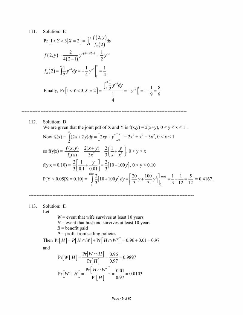
Pr Pr 0.14
Pr 0.22
Pr 0.12c c
C T
C T
C T
= +
=
=
∩
∩
Therefore, [ ] [ ] [ ] [ ]
[ ] [ ][ ]
0.88 1 Pr Pr Pr Pr Pr
Pr 0.14 Pr 0.22
2Pr 0.08
c cC T C T C T C T
T T
T
⎡ ⎤= − = = + −⎣ ⎦= + + −
= −
∩ ∪ ∩
or [ ] ( )Pr 0.88 0.08 2 0.48T = + =
9. Solution: B Let
event that customer insures more than one car
event that customer insures a sports carMS
==
Then applying DeMorgan’s Law, we may compute the desired probability as follows:
( ) ( ) ( ) ( ) ( ) ( )
( ) ( ) ( ) ( ) ( )( )
Pr Pr 1 Pr 1 Pr Pr Pr
1 Pr Pr Pr Pr 1 0.70 0.20 0.15 0.70 0.205
cc cM S M S M S M S M S
M S S M M
⎡ ⎤∩ = ∪ = − ∪ = − + − ∩⎡ ⎤⎣ ⎦⎣ ⎦= − − + = − − + =
-------------------------------------------------------------------------------------------------------- 10. Solution: C
Consider the following events about a randomly selected auto insurance customer: A = customer insures more than one car B = customer insures a sports car We want to find the probability of the complement of A intersecting the complement of B (exactly one car, non-sports). But P ( Ac ∩ Bc) = 1 – P (A ∪ B) And, by the Additive Law, P ( A ∪ B ) = P ( A) + P ( B ) – P ( A ∩ B ). By the Multiplicative Law, P ( A ∩ B ) = P ( B | A ) P (A) = 0.15 * 0.64 = 0.096 It follows that P ( A ∪ B ) = 0.64 + 0.20 – 0.096 = 0.744 and P (Ac ∩ Bc ) = 0.744 = 0.256
-------------------------------------------------------------------------------------------------------- 11. Solution: B
Let C = Event that a policyholder buys collision coverage D = Event that a policyholder buys disability coverage Then we are given that P[C] = 2P[D] and P[C ∩ D] = 0.15 . By the independence of C and D, it therefore follows that 0.15 = P[C ∩ D] = P[C] P[D] = 2P[D] P[D] = 2(P[D])2 (P[D])2 = 0.15/2 = 0.075 P[D] = 0.075 and P[C] = 2P[D] = 2 0.075 Now the independence of C and D also implies the independence of CC and DC . As a result, we see that P[CC ∩ DC] = P[CC] P[DC] = (1 – P[C]) (1 – P[D]) = (1 – 2 0.075 ) (1 – 0.075 ) = 0.33 .
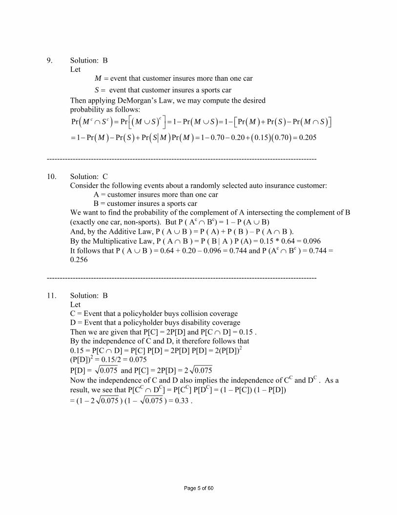
12. Solution: E
“Boxed” numbers in the table below were computed. High BP Low BP Norm BP Total Regular heartbeat 0.09 0.20 0.56 0.85 Irregular heartbeat 0.05 0.02 0.08 0.15 Total 0.14 0.22 0.64 1.00
From the table, we can see that 20% of patients have a regular heartbeat and low blood pressure.
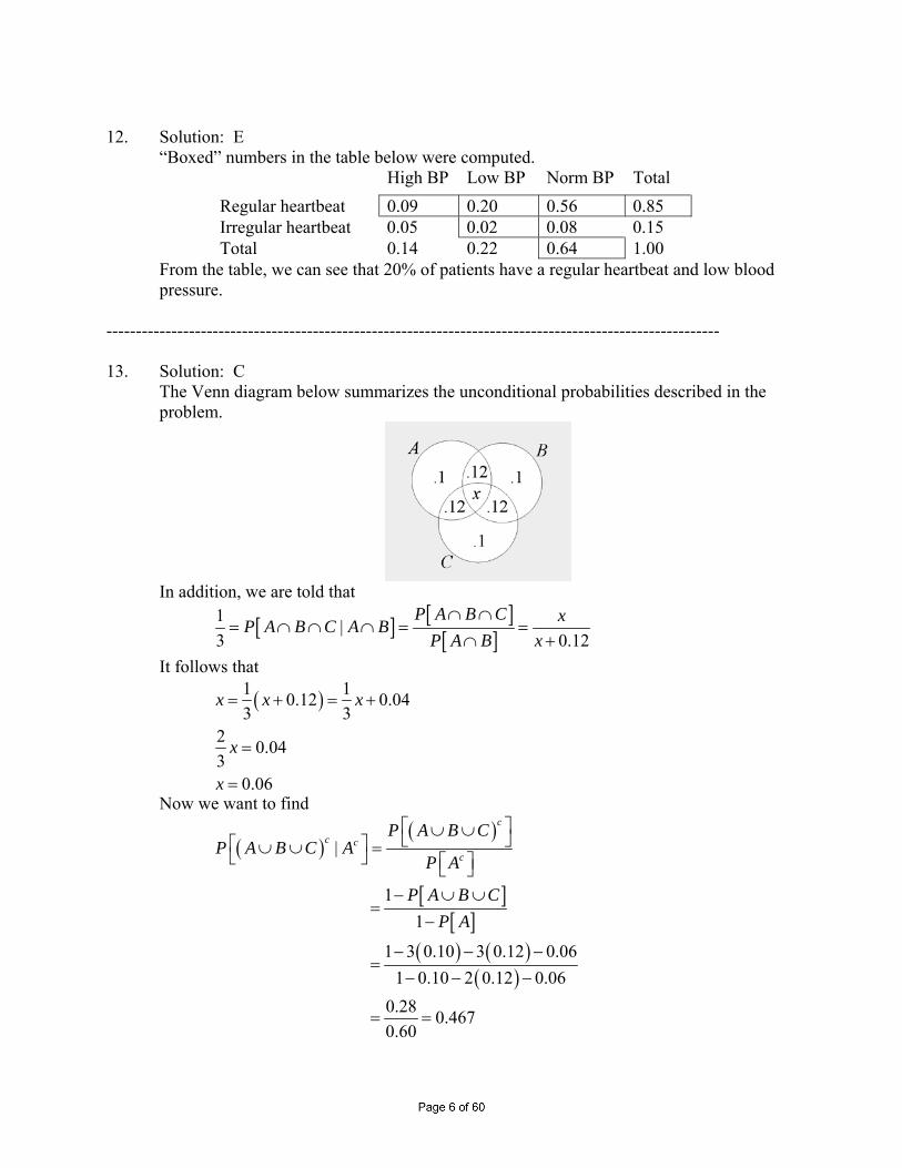
-------------------------------------------------------------------------------------------------------- 13. Solution: C
The Venn diagram below summarizes the unconditional probabilities described in the problem.
In addition, we are told that
[ ] [ ][ ]
1 |3 0.12
P A B C xP A B C A BP A B x∩ ∩
= ∩ ∩ ∩ = =∩ +
It follows that
( )1 10.12 0.043 3
2 0.043
0.06
x x x
x
x
= + = +
=
=
Now we want to find
( )( )
[ ][ ]
( ) ( )( )
|
1
1
1 3 0.10 3 0.12 0.06
1 0.10 2 0.12 0.060.28 0.4670.60
c
c cc
P A B CP A B C A
P A
P A B CP A
⎡ ⎤∪ ∪⎣ ⎦⎡ ⎤∪ ∪ =⎣ ⎦ ⎡ ⎤⎣ ⎦− ∪ ∪
=−
− − −=
− − −
= =
14. Solution: A
pk = 1 2 3 01 1 1 1 1 1 1... 05 5 5 5 5 5 5
k
k k kp p p p k− − −⎛ ⎞= = ⋅ ⋅ = = ≥⎜ ⎟⎝ ⎠
1 = 00 0
0 0
1 515 415
k
kk k
pp p p∞ ∞
= =
⎛ ⎞= = =⎜ ⎟⎝ ⎠ −
∑ ∑
p0 = 4/5 . Therefore, P[N > 1] = 1 – P[N ≤1] = 1 – (4/5 + 4/5 ⋅ 1/5) = 1 – 24/25 = 1/25 = 0.04 .
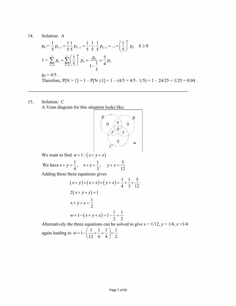
-------------------------------------------------------------------------------------------------------- 15. Solution: C A Venn diagram for this situation looks like:
We want to find ( )1w x y z= − + +
1 1 5We have , , 4 3 12
x y x z y z+ = + = + =
Adding these three equations gives
( ) ( ) ( )
( )
( )
1 1 54 3 12
2 112
1 11 12 2
x y x z y z
x y z
x y z
w x y z
+ + + + + = + +
+ + =
+ + =
= − + + = − =
Alternatively the three equations can be solved to give x = 1/12, y = 1/6, z =1/4
again leading to 1 1 1 1112 6 4 2
w ⎛ ⎞= − + + =⎜ ⎟⎝ ⎠
16. Solution: D Let 1 2 and N N denote the number of claims during weeks one and two, respectively.
Then since 1 2 and N N are independent,
[ ] [ ] [ ]71 2 1 20
7
1 80
7
90
9 6
Pr 7 Pr Pr 7
1 1 2 2
1 2
8 1 1 2 2 64
n
n nn
n
N N N n N n=
+ −=
=
+ = = = = −
⎛ ⎞⎛ ⎞= ⎜ ⎟⎜ ⎟⎝ ⎠⎝ ⎠
=
= = =
∑
∑
∑
-------------------------------------------------------------------------------------------------------- 17. Solution: D Let
Event of operating room chargesEvent of emergency room charges
OE==
Then
( ) ( ) ( ) ( )
( ) ( ) ( ) ( ) ( )0.85 Pr Pr Pr Pr
Pr Pr Pr Pr Independence
O E O E O E
O E O E
= ∪ = + − ∩
= + −
Since ( ) ( )Pr 0.25 1 PrcE E= = − , it follows ( )Pr 0.75E = .
So ( ) ( )( )0.85 Pr 0.75 Pr 0.75O O= + −
( )( )Pr 1 0.75 0.10O − =
( )Pr 0.40O = -------------------------------------------------------------------------------------------------------- 18. Solution: D
Let X1 and X2 denote the measurement errors of the less and more accurate instruments, respectively. If N(μ,σ) denotes a normal random variable with mean μ and standard deviation σ, then we are given X1 is N(0, 0.0056h), X2 is N(0, 0.0044h) and X1, X2 are
independent. It follows that Y = 2 2 2 2
1 2 0.0056 0.0044is N (0, )2 4
X X h h+ + = N(0,
0.00356h) . Therefore, P[−0.005h ≤ Y ≤ 0.005h] = P[Y ≤ 0.005h] – P[Y ≤ −0.005h] = P[Y ≤ 0.005h] – P[Y ≥ 0.005h]
= 2P[Y ≤ 0.005h] – 1 = 2P 0.0050.00356
hZh
⎡ ⎤≤⎢ ⎥⎣ ⎦ − 1 = 2P[Z ≤ 1.4] – 1 = 2(0.9192) – 1 = 0.84.
19. Solution: B Apply Bayes’ Formula. Let Event of an accidentA = 1B =Event the driver’s age is in the range 16-20 2B =Event the driver’s age is in the range 21-30 3B = Event the driver’s age is in the range 30-65 4B = Event the driver’s age is in the range 66-99 Then
( ) ( ) ( )
( ) ( ) ( ) ( ) ( ) ( ) ( ) ( )( )( )
( )( ) ( )( ) ( )( ) ( )( )
1 11
1 1 2 2 3 3 4 4
Pr PrPr
Pr Pr Pr Pr Pr Pr Pr Pr
0.06 0.080.1584
0.06 0.08 0.03 0.15 0.02 0.49 0.04 0.28
A B BB A
A B B A B B A B B A B B=
+ + +
= =+ + +
-------------------------------------------------------------------------------------------------------- 20. Solution: D
Let S = Event of a standard policy F = Event of a preferred policy U = Event of an ultra-preferred policy D = Event that a policyholder dies
Then
[ ] [ ] [ ][ ] [ ] [ ] [ ] [ ] [ ]
( ) ( )( ) ( ) ( ) ( ) ( ) ( )
||
| | |
0.001 0.10
0.01 0.50 0.005 0.40 0.001 0.10 0.0141
P D U P UP U D
P D S P S P D F P F P D U P U=
+ +
=+ +
=
-------------------------------------------------------------------------------------------------------- 21. Solution: B Apply Baye’s Formula:
[ ][ ] [ ] [ ]
( )( )( )( ) ( )( ) ( )( )
Pr Seri. Surv.
Pr Surv. Seri. Pr Seri.Pr Surv. Crit. Pr Crit. Pr Surv. Seri. Pr Seri. Pr Surv. Stab. Pr Stab.
0.9 0.30.29
0.6 0.1 0.9 0.3 0.99 0.6
⎡ ⎤⎣ ⎦⎡ ⎤⎣ ⎦=
⎡ ⎤ + ⎡ ⎤ + ⎡ ⎤⎣ ⎦ ⎣ ⎦ ⎣ ⎦
= =+ +
22. Solution: D Let
Event of a heavy smokerEvent of a light smokerEvent of a non-smokerEvent of a death within five-year period
HLND
====
Now we are given that 1Pr 2 Pr and Pr Pr2
D L D N D L D H⎡ ⎤ = ⎡ ⎤ ⎡ ⎤ = ⎡ ⎤⎣ ⎦ ⎣ ⎦ ⎣ ⎦ ⎣ ⎦
Therefore, upon applying Bayes’ Formula, we find that
[ ][ ] [ ] [ ]
( )
( ) ( ) ( )
Pr PrPr
Pr Pr Pr Pr Pr Pr
2 Pr 0.2 0.4 0.421 0.25 0.3 0.4Pr 0.5 Pr 0.3 2 Pr 0.22
D H HH D
D N N D L L D H H
D L
D L D L D L
⎡ ⎤⎣ ⎦⎡ ⎤ =⎣ ⎦ ⎡ ⎤ + ⎡ ⎤ + ⎡ ⎤⎣ ⎦ ⎣ ⎦ ⎣ ⎦⎡ ⎤⎣ ⎦= = =
+ +⎡ ⎤ + ⎡ ⎤ + ⎡ ⎤⎣ ⎦ ⎣ ⎦ ⎣ ⎦
-------------------------------------------------------------------------------------------------------- 23. Solution: D
Let C = Event of a collision T = Event of a teen driver Y = Event of a young adult driver M = Event of a midlife driver S = Event of a senior driver Then using Bayes’ Theorem, we see that
P[Y⏐C] = [ ] [ ]
[ ] [ ] [ ] [ ] [ ] [ ] [ ] [ ]
P C Y P Y
P C T P T P C Y P Y P C M P M P C S P S+ + +
= (0.08)(0.16)(0.15)(0.08) (0.08)(0.16) (0.04)(0.45) (0.05)(0.31)+ + +
= 0.22 .
-------------------------------------------------------------------------------------------------------- 24. Solution: B Observe
[ ][ ]
Pr 1 4 1 1 1 1 1 1 1 1 1Pr 1 46 12 20 30 2 6 12 20 30Pr 4
10 5 3 2 20 230 10 5 3 2 50 5
NN N
N≤ ≤ ⎡ ⎤ ⎡ ⎤⎡ ≥ ≤ ⎤ = = + + + + + + +⎣ ⎦ ⎢ ⎥ ⎢ ⎥≤ ⎣ ⎦ ⎣ ⎦+ + +
= = =+ + + +
25. Solution: B
Let Y = positive test result D = disease is present (and ~D = not D)
Using Baye’s theorem:
P[D|Y] = [ | ] [ ] (0.95)(0.01)[ | ] [ ] [ |~ ] [~ ] (0.95)(0.01) (0.005)(0.99)
P Y D P DP Y D P D P Y D P D
=+ +
= 0.657 .
--------------------------------------------------------------------------------------------------------
26. Solution: C Let: S = Event of a smoker C = Event of a circulation problem Then we are given that P[C] = 0.25 and P[S⏐C] = 2 P[S⏐CC]
Now applying Bayes’ Theorem, we find that P[C⏐S] = [ ] [ ]
[ ] [ ] [ ]( [ ])C C
P S C P C
P S C P C P S C P C+
= 2 [ ] [ ] 2(0.25) 2 2
2(0.25) 0.75 2 3 52 [ ] [ ] [ ](1 [ ])
C
C C
P S C P C
P S C P C P S C P C= = =
+ ++ − .
--------------------------------------------------------------------------------------------------------
27. Solution: D Use Baye’s Theorem with A = the event of an accident in one of the years 1997, 1998 or 1999.
P[1997|A] = [ 1997] [1997]
[ 1997][ [1997] [ 1998] [1998] [ 1999] [1999]P A P
P A P P A P P A P+ +
= (0.05)(0.16)(0.05)(0.16) (0.02)(0.18) (0.03)(0.20)+ +
= 0.45 .
--------------------------------------------------------------------------------------------------------
28. Solution: A
Let C = Event that shipment came from Company X I1 = Event that one of the vaccine vials tested is ineffective
Then by Bayes’ Formula, [ ] [ ] [ ][ ] [ ]
11
1 1
||
| | c c
P I C P CP C I
P I C P C P I C P C=
⎡ ⎤ ⎡ ⎤+ ⎣ ⎦ ⎣ ⎦
Now
[ ]
[ ]
[ ] ( ) ( ) ( )
( ) ( ) ( )
29301 1
29301 1
15
1 41 15 5
| 0.10 0.90 0.141
| 0.02 0.98 0.334
c
c
P C
P C P C
P I C
P I C
=
⎡ ⎤ = − = − =⎣ ⎦
= =
⎡ ⎤ = =⎣ ⎦
Therefore,
[ ] ( ) ( )( ) ( ) ( ) ( )1
0.141 1/ 5| 0.096
0.141 1/ 5 0.334 4 / 5P C I = =
+
-------------------------------------------------------------------------------------------------------- 29. Solution: C
Let T denote the number of days that elapse before a high-risk driver is involved in an accident. Then T is exponentially distributed with unknown parameter λ . Now we are given that
0.3 = P[T ≤ 50] = 50
50
00
t te dt eλ λλ − −= −∫ = 1 – e–50λ
Therefore, e–50λ = 0.7 or λ = − (1/50) ln(0.7)
It follows that P[T ≤ 80] = 80
800
0
t te dt eλ λλ − −= −∫ = 1 – e–80λ
= 1 – e(80/50) ln(0.7) = 1 – (0.7)80/50 = 0.435 . --------------------------------------------------------------------------------------------------------
30. Solution: D
Let N be the number of claims filed. We are given P[N = 2] = 2 4
32! 4!
e eλ λλ λ− −
= = 3 ⋅ P[N
= 4]24 λ2 = 6 λ4 λ2 = 4 ⇒ λ = 2 Therefore, Var[N] = λ = 2 .
31. Solution: D Let X denote the number of employees that achieve the high performance level. Then X
follows a binomial distribution with parameters 20 and 0.02n p= = . Now we want to determine x such that
[ ]Pr 0.01X x> ≤ or, equivalently,
[ ] ( )( ) ( )20200
0.99 Pr 0.02 0.98x k kkk
X x −
=≤ ≤ =∑
The following table summarizes the selection process for x: [ ] [ ]
( )( )( )( ) ( )
20
19
2 18
Pr Pr
0 0.98 0.668 0.668
1 20 0.02 0.98 0.272 0.940
2 190 0.02 0.98 0.0
x X x X x= ≤
=
=
= 53 0.993
Consequently, there is less than a 1% chance that more than two employees will achieve the high performance level. We conclude that we should choose the payment amount C such that
2 120,000C = or
60,000C = -------------------------------------------------------------------------------------------------------- 32. Solution: D
Let X = number of low-risk drivers insured Y = number of moderate-risk drivers insured Z = number of high-risk drivers insured f(x, y, z) = probability function of X, Y, and Z
Then f is a trinomial probability function, so [ ] ( ) ( ) ( ) ( )
( ) ( ) ( ) ( ) ( ) ( ) ( )4 3 3 2 2
Pr 2 0,0, 4 1,0,3 0,1,3 0, 2, 24! 0.20 4 0.50 0.20 4 0.30 0.20 0.30 0.20
2!2! 0.0488
z x f f f f≥ + = + + +
= + + +
=
33. Solution: B Note that
[ ] ( )20 2 20
2 2
1Pr 0.005 20 0.005 202
1 10.005 400 200 20 0.005 200 202 2
xxX x t dt t t
x x x x
⎛ ⎞> = − = −⎜ ⎟⎝ ⎠
⎛ ⎞ ⎛ ⎞= − − + = − +⎜ ⎟ ⎜ ⎟⎝ ⎠ ⎝ ⎠
∫
where 0 20x< < . Therefore,
[ ][ ]
( ) ( )( ) ( )
2
2
1200 20 16 16Pr 16 8 12Pr 16 81Pr 8 72 9200 20 8 82
XX X
X
− +>⎡ > > ⎤ = = = =⎣ ⎦ > − +
-------------------------------------------------------------------------------------------------------- 34. Solution: C
We know the density has the form ( ) 210C x −+ for 0 40x< < (equals zero otherwise).
First, determine the proportionality constant C from the condition 40
0( ) 1f x dx=∫ :
( )4040 2 1
0 0
21 10 (10 )10 50 25C CC x dx C x C− −= + =− + = − =∫
so 25 2C = , or 12.5 . Then, calculate the probability over the interval (0, 6):
( ) ( ) ( )66 2 1
0 0
1 112.5 10 10 12.5 0.4710 16
x dx x− − ⎛ ⎞+ = − + = − =⎜ ⎟⎝ ⎠∫ .
-------------------------------------------------------------------------------------------------------- 35. Solution: C
Let the random variable T be the future lifetime of a 30-year-old. We know that the density of T has the form f (x) = C(10 + x)−2 for 0 < x < 40 (and it is equal to zero otherwise). First, determine the proportionality constant C from the condition
400 ( ) 1:f x dx∫ =
1 = 40 1 40
00
2( ) (10 ) |25
f x dx C x C−=− + =∫
so that C = 252
= 12.5. Then, calculate P(T < 5) by integrating f (x) = 12.5 (10 + x)−2
over the interval (0.5).
36. Solution: B
To determine k, note that
1 = ( ) ( )1
4 5 1
00
1 15 5k kk y dy y− = − − =∫
k = 5 We next need to find P[V > 10,000] = P[100,000 Y > 10,000] = P[Y > 0.1]
= ( ) ( )1
4 5 10.1
0.1
5 1 1y dy y− = − −∫ = (0.9)5 = 0.59 and P[V > 40,000]
= P[100,000 Y > 40,000] = P[Y > 0.4] = ( ) ( )1
4 5 10.4
0.4
5 1 1y dy y− = − −∫ = (0.6)5 = 0.078 .
It now follows that P[V > 40,000⏐V > 10,000]
= [ 40,000 10,000] [ 40,000] 0.078[ 10,000] [ 10,000] 0.590
P V V P VP V P V
> ∩ > >= =
> > = 0.132 .
--------------------------------------------------------------------------------------------------------
37. Solution: D Let T denote printer lifetime. Then f(t) = ½ e–t/2, 0 ≤ t ≤ ∞ Note that
P[T ≤ 1] = 1
/ 2 / 2 1
00
12
t te dt e− −=∫ = 1 – e–1/2 = 0.393
P[1 ≤ T ≤ 2] = 2
2/ 2 / 21
1
12
t te dt e− −=∫ = e –1/2 − e –1 = 0.239
Next, denote refunds for the 100 printers sold by independent and identically distributed random variables Y1, . . . , Y100 where
200 with probability 0.393100 with probability 0.239 i = 1, . . . , 1000 with probability 0.368
iY⎧⎪= ⎨⎪⎩
Now E[Yi] = 200(0.393) + 100(0.239) = 102.56
Therefore, Expected Refunds = [ ]100
1i
iE Y
=∑ = 100(102.56) = 10,256 .
38. Solution: A
Let F denote the distribution function of f. Then
( ) [ ] 4 3 3
11Pr 3 1
x xF x X x t dt t x− − −= ≤ = = − = −∫
Using this result, we see
[ ] ( ) ( )[ ]
[ ] [ ][ ]
( ) ( )( )
( ) ( )( )
3 3 3
3
Pr 2 1.5 Pr 2 Pr 1.5Pr 2 1.5
Pr 1.5 Pr 1.5
2 1.5 1.5 2 3 1 0.5781 1.5 41.5
X X X XX X
X X
F FF
− −
−
∩ ≥⎡ ⎤ − ≤⎣ ⎦≥ = =≥ ≥
− − ⎛ ⎞= = = − =⎜ ⎟− ⎝ ⎠
< << |
--------------------------------------------------------------------------------------------------------
39. Solution: E Let X be the number of hurricanes over the 20-year period. The conditions of the problem give x is a binomial distribution with n = 20 and p = 0.05 . It follows that P[X < 2] = (0.95)20(0.05)0 + 20(0.95)19(0.05) + 190(0.95)18(0.05)2 = 0.358 + 0.377 + 0.189 = 0.925 .
-------------------------------------------------------------------------------------------------------- 40. Solution: B Denote the insurance payment by the random variable Y. Then
0 if 0
if C 1X C
YX C X
< ≤⎧= ⎨ − < <⎩
Now we are given that
( ) ( ) ( )0.50.5 22
0 00.64 Pr 0.5 Pr 0 0.5 2 0.5
CCY X C x dx x C
++= < = < < + = = = +∫
Therefore, solving for C, we find 0.8 0.5C = ± − Finally, since 0 1C< < , we conclude that 0.3C =
41. Solution: E
Let X = number of group 1 participants that complete the study. Y = number of group 2 participants that complete the study.
Now we are given that X and Y are independent. Therefore,
( ) ( ) ( ) ( ){ }( ) ( ) ( ) ( )( ) ( )[ ] [ ][ ] [ ][ ] [ ]( )( )10
9
9 9 9 9
9 9 9 9
2 9 9 (due to symmetry)
2 9 9
2 9 9 (again due to symmetry)
2 9 1 9
2 0.
P X Y X Y
P X Y P X Y
P X Y
P X P Y
P X P X
P X P X
≥ ∩ ∪ ∩ ≥⎡ ⎤ ⎡ ⎤⎣ ⎦ ⎣ ⎦
= ≥ ∩ + ∩ ≥⎡ ⎤ ⎡ ⎤⎣ ⎦ ⎣ ⎦= ≥ ∩⎡ ⎤⎣ ⎦= ≥
= ≥
= ≥ − ≥
=
< <
< <
<
<
<
( ) ( ) ( ) ( ) ( ) ( ) ( ) ( ) ( )[ ][ ]
9 10 9 1010 10 1010 9 102 0.8 0.8 1 0.2 0.8 0.8
2 0.376 1 0.376 0.469
⎡ ⎤ ⎡ ⎤+ − −⎣ ⎦ ⎣ ⎦= − =
-------------------------------------------------------------------------------------------------------- 42. Solution: D
Let IA = Event that Company A makes a claim IB = Event that Company B makes a claim XA = Expense paid to Company A if claims are made XB = Expense paid to Company B if claims are made
Then we want to find ( ) ( ){ }
( ) ( )[ ] [ ] [ ] [ ]
( ) ( ) ( ) ( ) [ ][ ]
Pr
Pr Pr
Pr Pr Pr Pr Pr (independence)
0.60 0.30 0.40 0.30 Pr 0
0.18 0.12Pr 0
CA B A B A B
CA B A B A B
CA B A B A B
B A
B A
I I I I X X
I I I I X X
I I I I X X
X X
X X
⎡ ⎤∩ ∪ ∩ ∩⎡ ⎤⎣ ⎦⎣ ⎦
⎡ ⎤= ∩ + ∩ ∩⎡ ⎤⎣ ⎦⎣ ⎦⎡ ⎤= +⎣ ⎦
= + − ≥
= + − ≥
<
<
<
Now B AX X− is a linear combination of independent normal random variables. Therefore, B AX X− is also a normal random variable with mean
[ ] [ ] [ ] 9,000 10,000 1,000B A B AM E X X E X E X= − = − = − = −
and standard deviation ( ) ( ) ( ) ( )2 2Var Var 2000 2000 2000 2B AX Xσ = + = + = It follows that
[ ]
[ ]
1000Pr 0 Pr ( is standard normal)2000 2
1 Pr2 2
1 1 Pr2 2
1 Pr 0.354
B AX X Z Z
Z
Z
Z
⎡ ⎤− ≥ = ≥⎢ ⎥⎣ ⎦⎡ ⎤= ≥⎢ ⎥⎣ ⎦
⎡ ⎤= − ⎢ ⎥⎣ ⎦= − <
<
1 0.638 0.362= − =
Finally, ( ) ( ){ } ( ) ( )Pr 0.18 0.12 0.362
0.223
CA B A B A BI I I I X X⎡ ⎤∩ ∪ ∩ ∩ = +⎡ ⎤⎣ ⎦⎣ ⎦
=
<
-------------------------------------------------------------------------------------------------------- 43. Solution: D If a month with one or more accidents is regarded as success and k = the number of
failures before the fourth success, then k follows a negative binomial distribution and the requested probability is
[ ] [ ] ( )
( ) ( ) ( ) ( )
433
0
4 0 1 2 33 4 5 60 1 2 3
4
3 2Pr 4 1 Pr 3 15 5
3 2 2 2 215 5 5 5 5
3 8 8 32 1 15 5 5 25
0.2898
kk
kk
k k +
=
⎛ ⎞ ⎛ ⎞≥ = − ≤ = − ⎜ ⎟ ⎜ ⎟⎝ ⎠ ⎝ ⎠
⎡ ⎤⎛ ⎞ ⎛ ⎞ ⎛ ⎞ ⎛ ⎞ ⎛ ⎞= − + + +⎢ ⎥⎜ ⎟ ⎜ ⎟ ⎜ ⎟ ⎜ ⎟ ⎜ ⎟⎝ ⎠ ⎝ ⎠ ⎝ ⎠ ⎝ ⎠ ⎝ ⎠⎢ ⎥⎣ ⎦
⎛ ⎞ ⎡ ⎤= − + + +⎜ ⎟ ⎢ ⎥⎝ ⎠ ⎣ ⎦=
∑
Alternatively the solution is
( ) ( ) ( )4 4 4 2 4 3
4 5 61 2 3
2 2 3 2 3 2 3 0.28985 5 5 5 5 5 5
⎛ ⎞ ⎛ ⎞ ⎛ ⎞ ⎛ ⎞ ⎛ ⎞ ⎛ ⎞+ + + =⎜ ⎟ ⎜ ⎟ ⎜ ⎟ ⎜ ⎟ ⎜ ⎟ ⎜ ⎟⎝ ⎠ ⎝ ⎠ ⎝ ⎠ ⎝ ⎠ ⎝ ⎠ ⎝ ⎠
which can be derived directly or by regarding the problem as a negative binomial distribution with
i) success taken as a month with no accidents ii) k = the number of failures before the fourth success, and iii) calculating [ ]Pr 3k ≤
44. Solution: C
If k is the number of days of hospitalization, then the insurance payment g(k) is
g(k) = {100 for 1, 2, 3300 50( 3) for 4, 5.
k kk k
=+ − =
Thus, the expected payment is 5
1 2 3 4 51
( ) 100 200 300 350 400k
k
g k p p p p p p=
= + + + +∑ =
( )1 100 5 200 4 300 3 350 2 400 115
× + × + × + × + × =220
-------------------------------------------------------------------------------------------------------- 45. Solution: D
Note that ( )0 42 2 3 30 4
2 02 0
8 64 56 2810 10 30 30 30 30 30 15x x x xE X dx dx
−−
= − + = − + = − + = =∫ ∫
-------------------------------------------------------------------------------------------------------- 46. Solution: D
The density function of T is
( ) / 31 , 03
tf t e t−= ∞< <
Therefore, [ ] ( )
2 /3 /3
0 2
/3 2 /3 /30 2 2
2/3 2 /3 /32
2/3
max ,2
2 3 3
2
2 2 2 3 2 3
t t
t t t
t
E X E T
te dt e dt
e te e dt
e e ee
∞− −
∞− − ∞ −
− − − ∞
−
= ⎡ ⎤⎣ ⎦
= +
= − − +
= − + + −
= +
∫ ∫
∫| |
|
47. Solution: D
Let T be the time from purchase until failure of the equipment. We are given that T is exponentially distributed with parameter λ = 10 since 10 = E[T] = λ . Next define the payment
P under the insurance contract by
for 0 1x for 1 320 for 3
x T
P T
T
≤ ≤⎧⎪⎪= < ≤⎨⎪
>⎪⎩
We want to find x such that
1000 = E[P] = 1
0 10x
∫ e–t/10 dt + 3
1
12 10x∫ e–t/10 dt =
1/10 /10 3
10 2
t txxe e− −− −
= −x e–1/10 + x – (x/2) e–3/10 + (x/2) e–1/10 = x(1 – ½ e–1/10 – ½ e–3/10) = 0.1772x . We conclude that x = 5644 .
-------------------------------------------------------------------------------------------------------- 48. Solution: E Let X and Y denote the year the device fails and the benefit amount, respectively. Then
the density function of X is given by ( ) ( ) ( )10.6 0.4 , 1,2,3...xf x x−= =
and ( )1000 5 if 1,2,3,4
0 if 4x x
yx
− =⎧⎪= ⎨>⎪⎩
It follows that [ ] ( ) ( )( ) ( ) ( ) ( ) ( )2 34000 0.4 3000 0.6 0.4 2000 0.6 0.4 1000 0.6 0.4
2694E Y = + + +
=
-------------------------------------------------------------------------------------------------------- 49. Solution: D Define ( )f X to be hospitalization payments made by the insurance policy. Then
( )
100 if 1, 2,3( )
300 25 3 if 4,5X X
f XX X
=⎧⎪= ⎨ + − =⎪⎩
and
( ) ( ) [ ]
[ ]
5
1Pr
5 4 3 2 1100 200 300 325 35015 15 15 15 15
1 640100 160 180 130 70 213.333 3
kE f X f k X k
=
= =⎡ ⎤⎣ ⎦
⎛ ⎞ ⎛ ⎞ ⎛ ⎞ ⎛ ⎞ ⎛ ⎞= + + + +⎜ ⎟ ⎜ ⎟ ⎜ ⎟ ⎜ ⎟ ⎜ ⎟⎝ ⎠ ⎝ ⎠ ⎝ ⎠ ⎝ ⎠ ⎝ ⎠
= + + + + = =
∑
-------------------------------------------------------------------------------------------------------- 50. Solution: C
Let N be the number of major snowstorms per year, and let P be the amount paid to
the company under the policy. Then Pr[N = n] = 3/ 2(3 / 2)
!
n en
−
, n = 0, 1, 2, . . . and
0 for 010,000( 1) for 1
NP
N N=⎧
= ⎨ − ≥⎩.
Now observe that E[P] = 3/ 2
1
(3 / 2)10,000( 1)!
n
n
enn
−∞
=
−∑
= 10,000 e–3/2 + 3/ 2
0
(3 / 2)10,000( 1)!
n
n
enn
−∞
=
−∑ = 10,000 e–3/2 + E[10,000 (N – 1)]
= 10,000 e–3/2 + E[10,000N] – E[10,000] = 10,000 e–3/2 + 10,000 (3/2) – 10,000 = 7,231 . -------------------------------------------------------------------------------------------------------- 51. Solution: C
Let Y denote the manufacturer’s retained annual losses.
Then for 0.6 2
2 for 2x x
Yx
< ≤⎧= ⎨ >⎩
and E[Y] = 2 22.5 2.5 2.5 2.5
3.5 3.5 2.5 2.5 20.6 2 0.6
2.5(0.6) 2.5(0.6) 2.5(0.6) 2(0.6)2x dx dx dxx x x x
∞∞⎡ ⎤ ⎡ ⎤
+ = −⎢ ⎥ ⎢ ⎥⎣ ⎦ ⎣ ⎦
∫ ∫ ∫
= 2.5 2.5 2.5 2.5 2.5
21.5 2.5 1.5 1.5 1.50.6
2.5(0.6) 2(0.6) 2.5(0.6) 2.5(0.6) (0.6)1.5 (2) 1.5(2) 1.5(0.6) 2x
− + = − + + = 0.9343 .
52. Solution: A
Let us first determine K. Observe that 1 1 1 1 60 30 20 15 12 1371 12 3 4 5 60 60
60137
K K K
K
+ + + +⎛ ⎞ ⎛ ⎞ ⎛ ⎞= + + + + = =⎜ ⎟ ⎜ ⎟ ⎜ ⎟⎝ ⎠ ⎝ ⎠ ⎝ ⎠
=
It then follows that [ ] [ ]
( )
Pr Pr Insured Suffers a Loss Pr Insured Suffers a Loss
60 30.05 , 1,...,5137 137
N n N n
NN N
= = ⎡ = ⎤⎣ ⎦
= = =
Now because of the deductible of 2, the net annual premium [ ]P E X= where 0 , if 2
2 , if 2N
XN N
≤⎧= ⎨ − >⎩
Then,
[ ] ( ) ( ) ( ) ( )5
3
3 1 3 32 1 2 3 0.0314137 137 137 4 137 5N
P E X NN=
⎡ ⎤ ⎡ ⎤⎛ ⎞= = − = + + =⎢ ⎥ ⎢ ⎥⎜ ⎟⎝ ⎠ ⎣ ⎦ ⎣ ⎦
∑
--------------------------------------------------------------------------------------------------------
53. Solution: D
Let W denote claim payments. Then for 1 10
10 for 10y y
Wy< ≤⎧
= ⎨ ≥⎩
It follows that E[W] = 10
10
3 3 2 1011 10
2 2 2 1010 y dy dyy y y y
∞∞
+ = − −∫ ∫ = 2 – 2/10 + 1/10 = 1.9 .
54. Solution: B
Let Y denote the claim payment made by the insurance company. Then
( )0 with probability 0.94Max 0, 1 with probability 0.0414 with probability 0.02
Y x⎧⎪= −⎨⎪⎩
and
[ ] ( ) ( ) ( ) ( ) ( ) ( ) ( )
( )
( )
( )
15 / 2
1
15 15/ 2 / 2
1 1
15 15/ 2 15 / 2 / 21 1 1
7.5 0.5 / 2
0.94 0 0.04 0.5003 1 0.02 14
0.020012 0.28
0.28 0.020012 2 2
0.28 0.020012 30 2
x
x x
x x x
x
E Y x e dx
xe dx e dx
xe e dx e dx
e e e d
−
− −
− − −
− − −
= + − +
⎡ ⎤= − +⎢ ⎥⎣ ⎦⎡ ⎤= + − + −⎢ ⎥⎣ ⎦
= + − + +
∫
∫ ∫
∫ ∫|
( )( ) ( )( ) ( )( ) ( )
15
1
7.5 0.5 / 2 151
7.5 0.5 7.5 0.5
7.5 0.5
0.28 0.020012 30 2 2
0.28 0.020012 30 2 2 2
0.28 0.020012 32 4
0.28 0.020012 2.408 0.328 (in tho
x
x
e e e
e e e e
e e
− − −
− − − −
− −
⎡ ⎤⎢ ⎥⎣ ⎦⎡ ⎤= + − + −⎣ ⎦
= + − + − +
= + − +
= +
=
∫|
usands)
It follows that the expected claim payment is 328 . --------------------------------------------------------------------------------------------------------
55. Solution: C
The pdf of x is given by f(x) = 4(1 )kx+
, 0 < x < ∞ . To find k, note
1 = 04 30
1(1 ) 3 (1 ) 3
k k kdxx x
∞∞
= − =+ +∫
k = 3
It then follows that E[x] = 40
3(1 )
x dxx
∞
+∫ and substituting u = 1 + x, du = dx, we see
E[x] = 41
3( 1)u duu
∞ −∫ = 3
2 33 4
1 1
1 1( ) 3 32 3 2 3
u uu u du∞∞ − −
− − ⎡ ⎤ ⎡ ⎤− = − = −⎢ ⎥ ⎢ ⎥− − ⎣ ⎦⎣ ⎦∫ = 3/2 – 1 = ½ .
56. Solution: C
Let Y represent the payment made to the policyholder for a loss subject to a deductible D.
That is 0 for 0
for 1X D
Yx D D X
≤ ≤⎧= ⎨ − < ≤⎩
Then since E[X] = 500, we want to choose D so that 1000 2 2
10001 1 1 ( ) (1000 )500 ( )4 1000 1000 2 2000D
D
x D Dx D dx − −= − = =∫
(1000 – D)2 = 2000/4 ⋅ 500 = 5002 1000 – D = ± 500 D = 500 (or D = 1500 which is extraneous).
-------------------------------------------------------------------------------------------------------- 57. Solution: B
We are given that Mx(t) = 4
1(1 2500 )t−
for the claim size X in a certain class of accidents.
First, compute Mx′(t) = 5 5
( 4)( 2500) 10,000(1 2500 ) (1 2500 )t t− −
=− −
Mx″(t) = 6 6
(10,000)( 5)( 2500) 125,000,000(1 2500 ) (1 2500 )t t
− −=
− −
Then E[X] = Mx′ (0) = 10,000 E[X2] = Mx″ (0) = 125,000,000 Var[X] = E[X2] – {E[X]}2 = 125,000,000 – (10,000)2 = 25,000,000 [ ]Var X = 5,000 .
--------------------------------------------------------------------------------------------------------
58. Solution: E Let XJ, XK, and XL represent annual losses for cities J, K, and L, respectively. Then X = XJ + XK + XL and due to independence M(t) = ( )J K L J K Lx x x t x t x t x txtE e E e E e E e E e+ +⎡ ⎤ ⎡ ⎤ ⎡ ⎤ ⎡ ⎤⎡ ⎤ = =⎣ ⎦ ⎣ ⎦ ⎣ ⎦⎣ ⎦⎣ ⎦
= MJ(t) MK(t) ML(t) = (1 – 2t)–3 (1 – 2t)–2.5 (1 – 2t)–4.5 = (1 – 2t)–10 Therefore, M′(t) = 20(1 – 2t)–11 M″(t) = 440(1 – 2t)–12 M″′(t) = 10,560(1 – 2t)–13 E[X3] = M″′(0) = 10,560
59. Solution: B The distribution function of X is given by
( ) ( ) ( ) ( )2.5 2.5 2.5
3.5 2.5 2.5200200
2.5 200 200 2001 , 200
xx
F x dt xt t x
−= = = − >∫
Therefore, the thp percentile px of X is given by
( ) ( )
( )
( )
( )
2.5
2.5
2.5
2.5
2 5
2 5
2001
100
2001 0.01
2001 0.01
2001 0.01
pp
p
p
p
p F xx
px
px
xp
= = −
− =
− =
=−
It follows that ( ) ( )70 30 2 5 2 5
200 200 93.060.30 0.70
x x− = − =
-------------------------------------------------------------------------------------------------------- 60. Solution: E
Let X and Y denote the annual cost of maintaining and repairing a car before and after the 20% tax, respectively. Then Y = 1.2X and Var[Y] = Var[1.2X] = (1.2)2 Var[X] = (1.2)2(260) = 374 .
-------------------------------------------------------------------------------------------------------- 61. Solution: A
The first quartile, Q1, is found by ¾ = Q1
∞z f(x) dx . That is, ¾ = (200/Q1)2.5 or
Q1 = 200 (4/3)0.4 = 224.4 . Similarly, the third quartile, Q3, is given by Q3 = 200 (4)0.4 = 348.2 . The interquartile range is the difference Q3 – Q1 .
62. Solution: C
First note that the density function of X is given by
( )
1 if 12
1 if 1 2
0 otherwise
x
x xf x
⎧ =⎪⎪⎪ − < <= ⎨⎪⎪⎪⎩
Then
( ) ( ) ( )
( ) ( ) ( )
( ) ( ) ( )
22 2 2 3 2
1 11
22 22 2 3 2 4 3
1 11
222
1 1 1 1 112 2 2 3 2
1 8 4 1 1 7 412 3 2 3 2 3 3
1 1 1 1 112 2 2 4 3
1 16 8 1 1 17 7 232 4 3 4 3 4 3 12
23 4 23 16 512 3 12 9 36
E X x x dx x x dx x x
E X x x dx x x dx x x
Var X E X E X
⎛ ⎞= + − = + − = + −⎜ ⎟⎝ ⎠
= + − − + = − =
⎛ ⎞= + − = + − = + −⎜ ⎟⎝ ⎠
= + − − + = − =
⎛ ⎞= − = − = − =⎡ ⎤ ⎜ ⎟⎣ ⎦ ⎝ ⎠
∫ ∫
∫ ∫
-------------------------------------------------------------------------------------------------------- 63. Solution: C
Note if 0 4
4 if 4 5X X
YX
≤ ≤⎧= ⎨ ≤⎩ <
Therefore,
[ ]
[ ] [ ]( )
4 5 2 4 50 40 4
4 52 2 3 4 50 40 4
222
1 4 1 45 5 10 5
16 20 16 8 4 12 10 5 5 5 5 5
1 16 1 165 5 15 5
64 80 64 64 16 64 48 112 15 5 5 15 5 15 15 15
112 12Var 1.7115 5
E Y xdx dx x x
E Y x dx dx x x
Y E Y E Y
= + = +
= + − = + =
⎡ ⎤ = + = +⎣ ⎦
= + − = + = + =
⎛ ⎞⎡ ⎤= − = − =⎜ ⎟⎣ ⎦ ⎝ ⎠
∫ ∫
∫ ∫
| |
| |
64. Solution: A
Let X denote claim size. Then E[X] = [20(0.15) + 30(0.10) + 40(0.05) + 50(0.20) + 60(0.10) + 70(0.10) + 80(0.30)] = (3 + 3 + 2 + 10 + 6 + 7 + 24) = 55 E[X2] = 400(0.15) + 900(0.10) + 1600(0.05) + 2500(0.20) + 3600(0.10) + 4900(0.10) + 6400(0.30) = 60 + 90 + 80 + 500 + 360 + 490 + 1920 = 3500 Var[X] = E[X2] – (E[X])2 = 3500 – 3025 = 475 and [ ]Var X = 21.79 . Now the range of claims within one standard deviation of the mean is given by [55.00 – 21.79, 55.00 + 21.79] = [33.21, 76.79] Therefore, the proportion of claims within one standard deviation is 0.05 + 0.20 + 0.10 + 0.10 = 0.45 .
-------------------------------------------------------------------------------------------------------- 65. Solution: B Let X and Y denote repair cost and insurance payment, respectively, in the event the auto
is damaged. Then 0 if 250
250 if 250x
Yx x
≤⎧= ⎨ − >⎩
and
[ ] ( ) ( )
( ) ( )
[ ] [ ]{ } ( )
[ ]
21500 2 1500250250
31500 2 32 1500250250
2 22
1 1 1250250 250 5211500 3000 3000
1 1 1250250 250 434,0281500 4500 4500
Var 434,028 521
Var 403
E Y x dx x
E Y x dx x
Y E Y E Y
Y
= − = − = =
⎡ ⎤ = − = − = =⎣ ⎦
⎡ ⎤= − = −⎣ ⎦
=
∫
∫
-------------------------------------------------------------------------------------------------------- 66. Solution: E
Let X1, X2, X3, and X4 denote the four independent bids with common distribution function F. Then if we define Y = max (X1, X2, X3, X4), the distribution function G of Y is given by
( ) [ ]( ) ( ) ( ) ( )[ ] [ ] [ ] [ ]( )
( )
1 2 3 4
1 2 3 4
4
4
Pr
Pr
Pr Pr Pr Pr
1 3 5 1 sin , 16 2 2
G y Y y
X y X y X y X y
X y X y X y X y
F y
y yπ
= ≤
= ≤ ∩ ≤ ∩ ≤ ∩ ≤⎡ ⎤⎣ ⎦= ≤ ≤ ≤ ≤
= ⎡ ⎤⎣ ⎦
= + ≤ ≤
It then follows that the density function g of Y is given by
( ) ( )
( ) ( )
( )
3
3
'1 1 sin cos4
3 5 cos 1 sin , 4 2 2
g y G y
y y
y y y
π π π
π π π
=
= +
= + ≤ ≤
Finally,
[ ] ( )
( )
5/ 2
3/ 2
5/ 2 3
3/ 2 cos 1 sin
4
E Y yg y dy
y y y dyπ π π
=
= +
∫
∫
-------------------------------------------------------------------------------------------------------- 67. Solution: B The amount of money the insurance company will have to pay is defined by the random
variable 1000 if 22000 if 2
x xY
x<⎧
= ⎨ ≥⎩
where x is a Poisson random variable with mean 0.6 . The probability function for X is
( ) ( )
[ ] ( )
( ) ( )
( ) ( )
0.6
0.6 0.62
0.6 0.6 0.6 0.60
0.6 0.6 0.6 0.6 0.6
0
0.60,1, 2,3 and
!0.60 1000 0.6 2000
!0.61000 0.6 2000 0.6
!
0.62000 2000 1000 0.6 2000 2000 600
!573
k
k
k
k
k
k
k
ep x k
k
E Y e ek
e e e ek
e e e e ek
−
∞− −=
∞− − − −=
∞− − − − −
=
= =
= + +
⎛ ⎞= + − −⎜ ⎟
⎝ ⎠
= − − = − −
=
∑
∑
∑
( ) ( ) ( )
( ) ( ) ( ) ( ) ( )
( ) ( ) ( ) ( ) ( )
[ ] [ ]{ } ( )
2 22 0.6 0.62
2 2 2 20.6 0.6 0.60
2 2 2 20.6 0.6
2 22
0.61000 0.6 2000!
0.6 2000 2000 2000 1000 0.6!
2000 2000 2000 1000 0.6
816,893
Var 816,893 573
k
k
k
k
E Y e ek
e e ek
e e
Y E Y E Y
∞− −=
∞− − −=
− −
⎡ ⎤ = +⎣ ⎦
⎡ ⎤= − − −⎣ ⎦
⎡ ⎤= − − −⎣ ⎦=
⎡ ⎤= − = −⎣ ⎦
∑
∑
[ ]
488,564
Var 699Y
=
=
68. Solution: C
Note that X has an exponential distribution. Therefore, c = 0.004 . Now let Y denote the
claim benefits paid. Then for 250
250 for 250x x
Yx<⎧
= ⎨ ≥⎩ and we want to find m such that 0.50
= 0.004 0.0040
0
0.004m
mx xe dx e− −= −∫ = 1 – e–0.004m
This condition implies e–0.004m = 0.5 ⇒ m = 250 ln 2 = 173.29 . -------------------------------------------------------------------------------------------------------- 69. Solution: D The distribution function of an exponential random variable T with parameter θ is given by ( ) 1 , 0tF t e tθ−= − >
Since we are told that T has a median of four hours, we may determine θ as follows:
( )
( )
( )
4
4
1 4 1212
4ln 2
4ln 2
F e
e
θ
θ
θ
θ
−
−
= = −
=
− = −
=
Therefore, ( ) ( )( )5ln 2
5 5 44Pr 5 1 5 2 0.42T F e eθ −− −≥ = − = = = = -------------------------------------------------------------------------------------------------------- 70. Solution: E
Let X denote actual losses incurred. We are given that X follows an exponential distribution with mean 300, and we are asked to find the 95th percentile of all claims that exceed 100 . Consequently, we want to find p95 such that
0.95 = 95 95Pr[100 ] ( ) (100)[ 100] 1 (100)
x p F p FP X F
< < −=
> − where F(x) is the distribution function of X .
Now F(x) = 1 – e–x/300 .
Therefore, 0.95 = 95 95
95
/300 /300100/300 1/3/3001/3
100/300 1/3
1 (1 ) 11 (1 )
p ppe e e e e e
e e
− −− −−
− −
− − − −= = −
− −
95 /300pe− = 0.05 e –1/3 p95 = −300 ln(0.05 e–1/3) = 999
71. Solution: A
The distribution function of Y is given by ( ) ( ) ( ) ( )2Pr Pr 1 4G y T y T y F y y= ≤ = ≤ = = −
for 4y > . Differentiate to obtain the density function ( ) 24g y y−= Alternate solution: Differentiate ( )F t to obtain ( ) 38f t t−= and set 2y t= . Then t y= and
( ) ( )( ) ( ) ( ) 3 2 1 2 218 42
dg y f t y dt dy f y y y y ydt
− − −⎛ ⎞= = = =⎜ ⎟⎝ ⎠
-------------------------------------------------------------------------------------------------------- 72. Solution: E We are given that R is uniform on the interval ( )0.04,0.08 and 10,000 RV e= Therefore, the distribution function of V is given by
( ) [ ] ( ) ( )( ) ( )
( ) ( )
( ) ( )ln ln 10,000
ln ln 10,000
0.040.04
Pr Pr 10,000 Pr ln ln 10,000
1 1 25ln 25ln 10,000 10.04 0.04
25 ln 0.0410,000
R
vv
F v V v e v R v
dr r v
v
−−
⎡ ⎤= ≤ = ≤ = ≤ −⎡ ⎤⎣ ⎦⎣ ⎦
= = = − −
⎡ ⎤⎛ ⎞= −⎢ ⎥⎜ ⎟⎝ ⎠⎣ ⎦
∫
-------------------------------------------------------------------------------------------------------- 73. Solution: E
( ) [ ] ( ) ( )10
81080.8 10Pr Pr 10 Pr 110
YYF y Y y X y X e−⎡ ⎤⎡ ⎤= ≤ = ≤ = ≤ = −⎢ ⎥⎣ ⎦ ⎣ ⎦
Therefore, ( ) ( ) ( )5 41
4101
8 10YYf y F y e−⎛ ⎞′= = ⎜ ⎟
⎝ ⎠
74. Solution: E
First note R = 10/T . Then
FR(r) = P[R ≤ r] = 10 10 101 TP r P T FT r r
⎡ ⎤ ⎡ ⎤ ⎛ ⎞≤ = ≥ = − ⎜ ⎟⎢ ⎥ ⎢ ⎥⎣ ⎦ ⎣ ⎦ ⎝ ⎠ . Differentiating with respect to
r fR(r) = F′R(r) = d/dr ( ) 2
10 101 T TdF F t
r dt r⎛ ⎞ −⎛ ⎞ ⎛ ⎞⎛ ⎞− = −⎜ ⎟ ⎜ ⎟⎜ ⎟⎜ ⎟⎝ ⎠ ⎝ ⎠⎝ ⎠⎝ ⎠
1( ) ( )4T T
d F t f tdt
= = since T is uniformly distributed on [8, 12] .
Therefore fR(r) = 2 2
1 10 54 2r r− −⎛ ⎞ =⎜ ⎟
⎝ ⎠ .
-------------------------------------------------------------------------------------------------------- 75. Solution: A
Let X and Y be the monthly profits of Company I and Company II, respectively. We are given that the pdf of X is f . Let us also take g to be the pdf of Y and take F and G to be the distribution functions corresponding to f and g . Then G(y) = Pr[Y ≤ y] = P[2X ≤ y] = P[X ≤ y/2] = F(y/2) and g(y) = G′(y) = d/dy F(y/2) = ½ F′(y/2) = ½ f(y/2) .
-------------------------------------------------------------------------------------------------------- 76. Solution: A
First, observe that the distribution function of X is given by
( ) 14 3 31
3 1 11 , 1x xF x dt xt t x
= = − = −∫ | >
Next, let X1, X2, and X3 denote the three claims made that have this distribution. Then if Y denotes the largest of these three claims, it follows that the distribution function of Y is given by
( ) [ ] [ ] [ ]1 2 3
3
3
Pr Pr Pr
1 1 , 1
G y X y X y X y
yy
= ≤ ≤ ≤
⎛ ⎞= −⎜ ⎟⎝ ⎠
>
while the density function of Y is given by
( ) ( )2 2
3 4 4 3
1 3 9 1' 3 1 1 , 1g y G y yy y y y
⎛ ⎞ ⎛ ⎞ ⎛ ⎞⎛ ⎞= = − = −⎜ ⎟ ⎜ ⎟ ⎜ ⎟⎜ ⎟
⎝ ⎠ ⎝ ⎠ ⎝ ⎠⎝ ⎠>
Therefore,
[ ]2
3 3 3 3 61 1
3 6 9 2 5 811
9 1 9 2 11 1
9 18 9 9 18 9 2 5 8
1 2 1 9 2.025 (in thousands)2 5 8
E Y dy dyy y y y y
dyy y y y y y
∞ ∞
∞∞
⎛ ⎞ ⎛ ⎞= − = − +⎜ ⎟ ⎜ ⎟
⎝ ⎠ ⎝ ⎠
⎛ ⎞ ⎡ ⎤= − + = − + −⎜ ⎟ ⎢ ⎥
⎝ ⎠ ⎣ ⎦
⎡ ⎤= − + =⎢ ⎥⎣ ⎦
∫ ∫
∫
-------------------------------------------------------------------------------------------------------- 77. Solution: D
Prob. = 1− 2 2
1 1
1 ( )8
x y dxdy+∫ ∫ = 0.625
Note
( ) ( ) ( ) ( ){ }( ) ( ) ( ) ( )
( ) ( ) ( ) ( ) ( )
2 2 2 2 211 1 1
2 2 2 3 3 211
Pr 1 1 Pr 1 1 (De Morgan's Law)
1 1 11 Pr 1 1 1 18 8 2
1 1 11 2 1 1 2 1 1 64 27 27 816 48 4818 301 0.62548 48
cX Y X Y
X Y x y dxdy x y dy
y y dy y y
≤ ≤ = > >⎡ ⎤ ⎡ ⎤⎣ ⎦ ⎣ ⎦
= − > > = − + = − +⎡ ⎤⎣ ⎦
⎡ ⎤ ⎡ ⎤= − + − + = − + − + = − − − +⎣ ⎦ ⎣ ⎦
= − = =
∫ ∫ ∫
∫
∪ ∩
∩
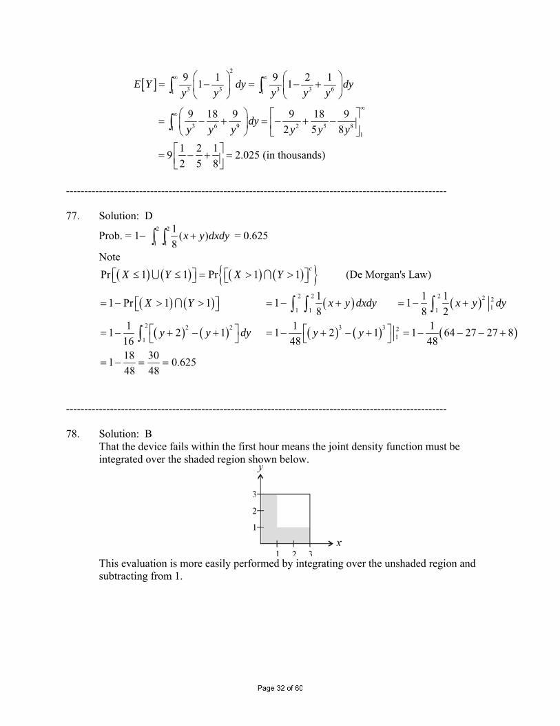
-------------------------------------------------------------------------------------------------------- 78. Solution: B
That the device fails within the first hour means the joint density function must be integrated over the shaded region shown below.
This evaluation is more easily performed by integrating over the unshaded region and subtracting from 1.
( ) ( )
( )
( ) ( ) ( )
323 3 3 3
1 1 1 11
33 2
11
Pr 1 1
2 11 1 1 9 6 1 227 54 54
1 1 1 32 111 8 4 1 8 2 1 24 18 8 2 1 0.4154 54 54 54 27
X Y
x y x xydx dy dy y y dy
y dy y y
< ∪ <⎡ ⎤⎣ ⎦
+ += − = − = − + − −
= − + = − + = − + − − = − = =
∫ ∫ ∫ ∫
∫
-------------------------------------------------------------------------------------------------------- 79. Solution: E
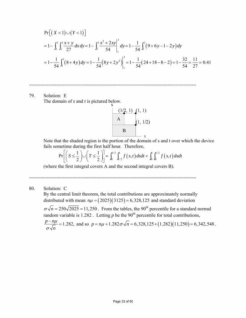
The domain of s and t is pictured below.
Note that the shaded region is the portion of the domain of s and t over which the device fails sometime during the first half hour. Therefore,
( ) ( )1/ 2 1 1 1/ 2
0 1/ 2 0 0
1 1Pr , ,2 2
S T f s t dsdt f s t dsdt⎡ ⎤⎛ ⎞ ⎛ ⎞≤ ∪ ≤ = +⎜ ⎟ ⎜ ⎟⎢ ⎥⎝ ⎠ ⎝ ⎠⎣ ⎦∫ ∫ ∫ ∫
(where the first integral covers A and the second integral covers B). -------------------------------------------------------------------------------------------------------- 80. Solution: C
By the central limit theorem, the total contributions are approximately normally distributed with mean ( )( )2025 3125 6,328,125nμ = = and standard deviation
250 2025 11,250nσ = = . From the tables, the 90th percentile for a standard normal random variable is 1.282 . Letting p be the 90th percentile for total contributions,
1.282,p nnμ
σ−
= and so ( )( )1.282 6,328,125 1.282 11,250 6,342,548p n nμ σ= + = + = .
-------------------------------------------------------------------------------------------------------- 81. Solution: C
Let X1, . . . , X25 denote the 25 collision claims, and let 125
X = (X1 + . . . +X25) . We are
given that each Xi (i = 1, . . . , 25) follows a normal distribution with mean 19,400 and standard deviation 5000 . As a result X also follows a normal distribution with mean
19,400 and standard deviation 125
(5000) = 1000 . We conclude that P[ X > 20,000]
= 19,400 20,000 19,400 19,400 0.61000 1000 1000
X XP P⎡ ⎤ ⎡ ⎤− − −> = >⎢ ⎥ ⎢ ⎥
⎣ ⎦ ⎣ ⎦ = 1 − Φ(0.6) = 1 – 0.7257
= 0.2743 . -------------------------------------------------------------------------------------------------------- 82. Solution: B
Let X1, . . . , X1250 be the number of claims filed by each of the 1250 policyholders. We are given that each Xi follows a Poisson distribution with mean 2 . It follows that E[Xi] = Var[Xi] = 2 . Now we are interested in the random variable S = X1 + . . . + X1250 . Assuming that the random variables are independent, we may conclude that S has an approximate normal distribution with E[S] = Var[S] = (2)(1250) = 2500 . Therefore P[2450 < S < 2600] =
2450 2500 2500 2600 2500 25001 2502500 2500 2500
2500 25002 150 50
S SP P
S SP P
− − − −⎡ ⎤ ⎡ ⎤< < = − < <⎢ ⎥ ⎢ ⎥⎣ ⎦⎣ ⎦− −⎡ ⎤ ⎡ ⎤= < − < −⎢ ⎥ ⎢ ⎥⎣ ⎦ ⎣ ⎦
Then using the normal approximation with Z = 250050
S − , we have P[2450 < S < 2600]
≈ P[Z < 2] – P[Z > 1] = P[Z < 2] + P[Z < 1] – 1 ≈ 0.9773 + 0.8413 – 1 = 0.8186 . -------------------------------------------------------------------------------------------------------- 83. Solution: B
Let X1,…, Xn denote the life spans of the n light bulbs purchased. Since these random variables are independent and normally distributed with mean 3 and variance 1, the random variable S = X1 + … + Xn is also normally distributed with mean
3nμ = and standard deviation
nσ = Now we want to choose the smallest value for n such that
[ ] 3 40 30.9772 Pr 40 Pr S n nSn n− −⎡ ⎤≤ = ⎢ ⎥⎣ ⎦
> >
This implies that n should satisfy the following inequality:
40 32 nn−
− ≥
To find such an n, let’s solve the corresponding equation for n:
( ) ( )
40 32
2 40 3
3 2 40 0
3 10 4 0
4 16
nn
n n
n n
n n
nn
−− =
− = −
− − =
+ − =
==
-------------------------------------------------------------------------------------------------------- 84. Solution: B Observe that
[ ] [ ] [ ][ ] [ ] [ ] [ ]
50 20 70
2 , 50 30 20 100
E X Y E X E Y
Var X Y Var X Var Y Cov X Y
+ = + = + =
+ = + + = + + =
for a randomly selected person. It then follows from the Central Limit Theorem that T is approximately normal with mean
[ ] ( )100 70 7000E T = = and variance
[ ] ( ) 2100 100 100Var T = = Therefore,
[ ]
[ ]
7000 7100 7000Pr 7100 Pr100 100
Pr 1 0.8413
TT
Z
− −⎡ ⎤< = <⎢ ⎥⎣ ⎦= < =
where Z is a standard normal random variable.
-------------------------------------------------------------------------------------------------------- 85. Solution: B
Denote the policy premium by P . Since x is exponential with parameter 1000, it follows from what we are given that E[X] = 1000, Var[X] = 1,000,000, [ ]Var X = 1000 and P = 100 + E[X] = 1,100 . Now if 100 policies are sold, then Total Premium Collected = 100(1,100) = 110,000 Moreover, if we denote total claims by S, and assume the claims of each policy are independent of the others then E[S] = 100 E[X] = (100)(1000) and Var[S] = 100 Var[X] = (100)(1,000,000) . It follows from the Central Limit Theorem that S is approximately normally distributed with mean 100,000 and standard deviation = 10,000 . Therefore,
P[S ≥ 110,000] = 1 – P[S ≤ 110,000] = 1 – 110,000 100,00010,000
P Z −⎡ ⎤≤⎢ ⎥⎣ ⎦ = 1 – P[Z ≤ 1] = 1
– 0.841 ≈ 0.159 . -------------------------------------------------------------------------------------------------------- 86. Solution: E Let 1 100,...,X X denote the number of pensions that will be provided to each new recruit.
Now under the assumptions given,
( )( )( )( )
0 with probability 1 0.4 0.61 with probability 0.4 0.25 0.1
2 with probability 0.4 0.75 0.3iX
⎧ − =⎪
= =⎨⎪ =⎩
for 1,...,100i = . Therefore, [ ] ( )( ) ( )( ) ( )( )
( ) ( ) ( ) ( ) ( ) ( )
[ ] [ ]{ } ( )
2 2 22
2 22
0 0.6 1 0.1 2 0.3 0.7 ,
0 0.6 1 0.1 2 0.3 1.3 , and
Var 1.3 0.7 0.81
i
i
i i i
E X
E X
X E X E X
= + + =
⎡ ⎤ = + + =⎣ ⎦
⎡ ⎤= − = − =⎣ ⎦
Since 1 100,...,X X are assumed by the consulting actuary to be independent, the Central Limit Theorem then implies that 1 100...S X X= + + is approximately normally distributed with mean
[ ] [ ] [ ] ( )1 100... 100 0.7 70E S E X E X= + + = = and variance
[ ] [ ] [ ] ( )1 100Var Var ... Var 100 0.81 81S X X= + + = = Consequently,
[ ]
[ ]
70 90.5 70Pr 90.5 Pr9 9
Pr 2.28 0.99
SS
Z
− −⎡ ⎤≤ = ≤⎢ ⎥⎣ ⎦= ≤
=
-------------------------------------------------------------------------------------------------------- 87. Solution: D
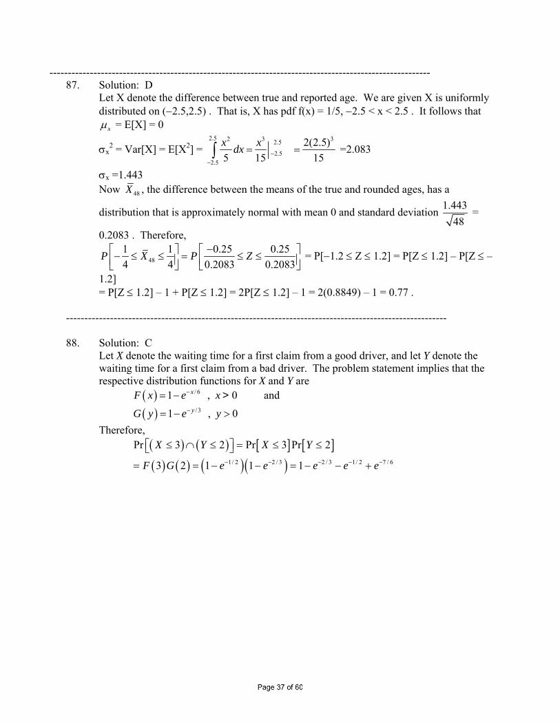
Let X denote the difference between true and reported age. We are given X is uniformly distributed on (−2.5,2.5) . That is, X has pdf f(x) = 1/5, −2.5 < x < 2.5 . It follows that
xμ = E[X] = 0
σx2 = Var[X] = E[X2] =
2.5 2 3 32.5
2.52.5
2(2.5)5 15 15x xdx −
−
= =∫ =2.083
σx =1.443 Now 48X , the difference between the means of the true and rounded ages, has a
distribution that is approximately normal with mean 0 and standard deviation 1.44348
=
0.2083 . Therefore,
481 1 0.25 0.254 4 0.2083 0.2083
P X P Z−⎡ ⎤ ⎡ ⎤− ≤ ≤ = ≤ ≤⎢ ⎥ ⎢ ⎥⎣ ⎦ ⎣ ⎦ = P[−1.2 ≤ Z ≤ 1.2] = P[Z ≤ 1.2] – P[Z ≤ –
1.2] = P[Z ≤ 1.2] – 1 + P[Z ≤ 1.2] = 2P[Z ≤ 1.2] – 1 = 2(0.8849) – 1 = 0.77 .
-------------------------------------------------------------------------------------------------------- 88. Solution: C
Let X denote the waiting time for a first claim from a good driver, and let Y denote the waiting time for a first claim from a bad driver. The problem statement implies that the respective distribution functions for X and Y are ( ) / 61 , 0xF x e x−= − > and
( ) /31 , 0yG y e y−= − > Therefore,
( ) ( ) [ ] [ ]( ) ( ) ( )( )1/ 2 2 / 3 2 / 3 1/ 2 7 / 6
Pr 3 2 Pr 3 Pr 2
3 2 1 1 1
X Y X Y
F G e e e e e− − − − −
≤ ∩ ≤ = ≤ ≤⎡ ⎤⎣ ⎦
= = − − = − − +
89. Solution: B
We are given that 6 (50 ) for 0 50 50
( , ) 125,0000 otherwise
x y x yf x y
⎧ − − < < − <⎪= ⎨⎪⎩
and we want to determine P[X > 20 ∩ Y > 20] . In order to determine integration limits, consider the following diagram:
y
x
50
50
(20, 30)
(30, 20)
x>20 y>20
We conclude that P[X > 20 ∩ Y > 20] = 30 50
20 20
6 (50 )125,000
x
x y−
− −∫ ∫ dy dx .
-------------------------------------------------------------------------------------------------------- 90. Solution: C
Let T1 be the time until the next Basic Policy claim, and let T2 be the time until the next Deluxe policy claim. Then the joint pdf of T1 and T2 is
1 2 1 2/ 2 /3 / 2 /31 2
1 1 1( , )2 3 6
t t t tf t t e e e e− − − −⎛ ⎞⎛ ⎞= =⎜ ⎟⎜ ⎟⎝ ⎠⎝ ⎠
, 0 < t1 < ∞ , 0 < t2 < ∞ and we need to find
P[T2 < T1] = 1
11 2 1 2/ 2 /3 / 2 /32 1 1
00 0 0
1 16 2
ttt t t te e dt dt e e dt
∞ ∞− − − −⎡ ⎤= −⎢ ⎥⎣ ⎦∫ ∫ ∫
= 1 1 1 1 1/ 2 / 2 /3 / 2 5 / 61 1
0 0
1 1 1 12 2 2 2
t t t t te e e dt e e dt∞ ∞
− − − − −⎡ ⎤ ⎡ ⎤− = −⎢ ⎥ ⎢ ⎥⎣ ⎦ ⎣ ⎦∫ ∫ = 1 1/ 2 5 / 6
0
3 3 215 5 5
t te e∞
− −⎡ ⎤− + = − =⎢ ⎥⎣ ⎦
= 0.4 . -------------------------------------------------------------------------------------------------------- 91. Solution: D
We want to find P[X + Y > 1] . To this end, note that P[X + Y > 1]
= 21 2 1
2
10 1 0
2 2 1 1 14 2 2 8 xx
x y dydx xy y y dx−−
+ −⎡ ⎤ ⎡ ⎤= + −⎢ ⎥ ⎢ ⎥⎣ ⎦ ⎣ ⎦∫ ∫ ∫
= 1
2
0
1 1 1 11 (1 ) (1 ) (1 )2 2 2 8
x x x x x dx⎡ ⎤+ − − − − − + −⎢ ⎥⎣ ⎦∫ = 1
2 2
0
1 1 1 12 8 4 8
x x x x dx⎡ ⎤+ + − +⎢ ⎥⎣ ⎦∫
= 1
2
0
5 3 18 4 8
x x dx⎡ ⎤+ +⎢ ⎥⎣ ⎦∫ = 1
3 2
0
5 3 124 8 8
x x x⎡ ⎤+ +⎢ ⎥⎣ ⎦ = 5 3 1 17
24 8 8 24+ + =
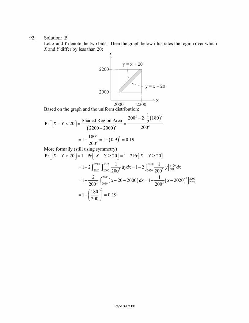
92. Solution: B Let X and Y denote the two bids. Then the graph below illustrates the region over which
X and Y differ by less than 20:
Based on the graph and the uniform distribution:
( )
( )
( )
22
2 2
22
2
1200 2 180Shaded Region Area 2Pr 202002200 2000
1801 1 0.9 0.19200
X Y− ⋅
⎡ − < ⎤ = =⎣ ⎦ −
= − = − =
More formally (still using symmetry)
[ ]
( ) ( )
2200 20 2200 2020002 22020 2000 2020
2200 2 220020202 22020
2
Pr 20 1 Pr 20 1 2Pr 20
1 11 2 1 2200 200
2 11 20 2000 1 2020200 2001801 0.19200
x x
X Y X Y X Y
dydx y dx
x dx x
− −
⎡ − < ⎤ = − ⎡ − ≥ ⎤ = − − ≥⎣ ⎦ ⎣ ⎦
= − = −
= − − − = − −
⎛ ⎞= − =⎜ ⎟⎝ ⎠
∫ ∫ ∫
∫
-------------------------------------------------------------------------------------------------------- 93. Solution: C
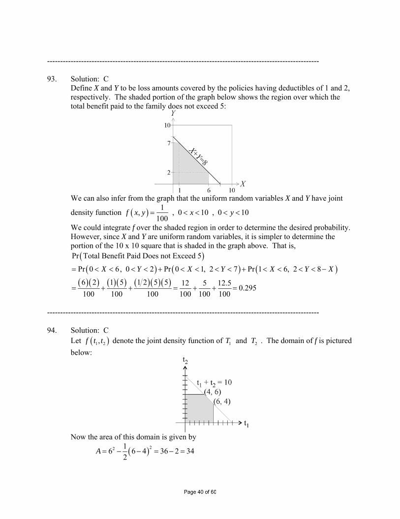
Define X and Y to be loss amounts covered by the policies having deductibles of 1 and 2, respectively. The shaded portion of the graph below shows the region over which the total benefit paid to the family does not exceed 5:
We can also infer from the graph that the uniform random variables X and Y have joint
density function ( ) 1, , 0 10 , 0 10100
f x y x y= < < < <
We could integrate f over the shaded region in order to determine the desired probability. However, since X and Y are uniform random variables, it is simpler to determine the portion of the 10 x 10 square that is shaded in the graph above. That is,
( )( ) ( ) ( )
( )( ) ( )( ) ( )( )( )
Pr Total Benefit Paid Does not Exceed 5
Pr 0 6, 0 2 Pr 0 1, 2 7 Pr 1 6, 2 8
6 2 1 5 1 2 5 5 12 5 12.5 0.295100 100 100 100 100 100
X Y X Y X Y X= < < < < + < < < < + < < < < −
= + + = + + =
-------------------------------------------------------------------------------------------------------- 94. Solution: C Let ( )1 2,f t t denote the joint density function of 1 2 and T T . The domain of f is pictured
below:
Now the area of this domain is given by
( )22 16 6 4 36 2 342
A = − − = − =
Consequently, ( ) 1 2 1 21 2
1 , 0 6 , 0 6 , 10, 34
0 elsewhere
t t t tf t t
⎧ < < < < + <⎪= ⎨⎪⎩
and [ ] [ ] [ ] [ ]
( )
11
1 2 1 2 1
4 6 6 10 4 6 1062 21 2 1 1 2 1 1 0 1 1 0 10 0 4 0 0 4
24 6 2 4 2 31 11 1 1 1 0 1 10 4
2 (due to symmetry)
1 12 234 34 34 34
3 31 1 12 10 2 517 34 34 34 3
t t
E T T E T E T E T
t tt dt dt t dt dt t dt t dt
t tdt t t dt t t
− −
+ = + =
⎧ ⎫⎡ ⎤ ⎡ ⎤⎧ ⎫= + = +⎨ ⎬ ⎨ ⎬⎢ ⎥ ⎢ ⎥⎩ ⎭ ⎣ ⎦ ⎣ ⎦⎩ ⎭
⎧ ⎫ ⎛= + − = + −⎨ ⎬ ⎜⎝⎩ ⎭
∫ ∫ ∫ ∫ ∫ ∫
∫ ∫ 64
24 1 642 180 72 80 5.717 34 3
⎧ ⎫⎞⎨ ⎬⎟
⎠⎩ ⎭⎧ ⎫⎡ ⎤= + − − + =⎨ ⎬⎢ ⎥⎣ ⎦⎩ ⎭
-------------------------------------------------------------------------------------------------------- 95. Solution: E
( ) ( ) ( ) ( ) ( )
( ) ( ) ( ) ( ) ( ) ( )
1 2 1 2 1 21 2
2 2 2 2 2 22 21 2 1 2 1 1 2 2 1 1 2 21 2 1 2 1 2
1 2
1 1 1 12 22 2 2 2
, t X Y t Y X t t X t t Yt W t Z
t t t t t t t t t t t tt t X t t Y t t
M t t E e E e E e e
E e E e e e e e e
+ + − − ++
− + − + + +− + +
⎡ ⎤ ⎡ ⎤⎡ ⎤= = =⎣ ⎦ ⎣ ⎦ ⎣ ⎦
⎡ ⎤ ⎡ ⎤= = = =⎣ ⎦ ⎣ ⎦
-------------------------------------------------------------------------------------------------------- 96. Solution: E
Observe that the bus driver collect 21x50 = 1050 for the 21 tickets he sells. However, he may be required to refund 100 to one passenger if all 21 ticket holders show up. Since passengers show up or do not show up independently of one another, the probability that all 21 passengers will show up is ( ) ( )21 211 0.02 0.98 0.65− = = . Therefore, the tour
operator’s expected revenue is ( ) ( )1050 100 0.65 985− = .
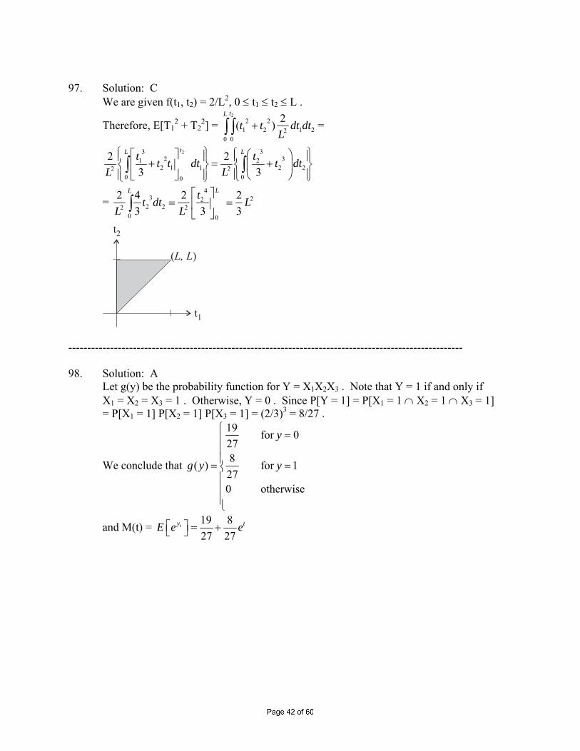
97. Solution: C
We are given f(t1, t2) = 2/L2, 0 ≤ t1 ≤ t2 ≤ L .
Therefore, E[T12 + T2
2] = 2
2 21 2 1 22
0 0
2( )tL
t t dt dtL
+∫ ∫ =
23 32 31 2
2 1 1 2 22 20 00
2 23 3
tL Lt tt t dt t dtL L
⎧ ⎫ ⎧ ⎫⎡ ⎤ ⎛ ⎞⎪ ⎪ ⎪ ⎪+ = +⎜ ⎟⎨ ⎬ ⎨ ⎬⎢ ⎥⎪ ⎪⎪ ⎪⎣ ⎦ ⎝ ⎠⎩ ⎭⎩ ⎭
∫ ∫
= 4
3 222 22 2
0 0
2 4 2 23 3 3
LL tt dt LL L
⎡ ⎤= =⎢ ⎥
⎣ ⎦∫
t2
( )L, L
t1 -------------------------------------------------------------------------------------------------------- 98. Solution: A
Let g(y) be the probability function for Y = X1X2X3 . Note that Y = 1 if and only if X1 = X2 = X3 = 1 . Otherwise, Y = 0 . Since P[Y = 1] = P[X1 = 1 ∩ X2 = 1 ∩ X3 = 1] = P[X1 = 1] P[X2 = 1] P[X3 = 1] = (2/3)3 = 8/27 .
We conclude that
19 for 0278( ) for 1270 otherwise
y
g y y
⎧ =⎪⎪⎪= =⎨⎪⎪⎪⎩
and M(t) = 19 827 27
ty tE e e⎡ ⎤ = +⎣ ⎦
99. Solution: C
( ) ( ) ( ) ( )( ) ( ) ( ) ( )
( ) ( ) ( )( )
2We use the relationships Var Var , Cov , Cov , , and
Var Var Var 2 Cov , . First we observe
17,000 Var 5000 10,000 2 Cov , , and so Cov , 1000.
We want to find Var 100 1.1 V
aX b a X aX bY ab X Y
X Y X Y X Y
X Y X Y X Y
X Y
+ = =
+ = + +
= + = + + =
+ + =⎡ ⎤⎣ ⎦ ( )[ ] ( ) ( )
( ) ( ) ( )2
ar 1.1 100
Var 1.1 Var Var 1.1 2 Cov ,1.1
Var 1.1 Var 2 1.1 Cov , 5000 12,100 2200 19,300.
X Y
X Y X Y X Y
X Y X Y
+ +⎡ ⎤⎣ ⎦= + = + +⎡ ⎤⎣ ⎦
= + + = + + =
-------------------------------------------------------------------------------------------------------- 100. Solution: B
Note P(X = 0) = 1/6 P(X = 1) = 1/12 + 1/6 = 3/12 P(X = 2) = 1/12 + 1/3 + 1/6 = 7/12 . E[X] = (0)(1/6) + (1)(3/12) + (2)(7/12) = 17/12 E[X2] = (0)2(1/6) + (1)2(3/12) + (2)2(7/12) = 31/12 Var[X] = 31/12 – (17/12)2 = 0.58 .
-------------------------------------------------------------------------------------------------------- 101. Solution: D
Note that due to the independence of X and Y Var(Z) = Var(3X − Y − 5) = Var(3X) + Var(Y) = 32 Var(X) + Var(Y) = 9(1) + 2 = 11 .
-------------------------------------------------------------------------------------------------------- 102. Solution: E
Let X and Y denote the times that the two backup generators can operate. Now the variance of an exponential random variable with mean 2is β β . Therefore,
[ ] [ ] 2Var Var 10 100X Y= = = Then assuming that X and Y are independent, we see
[ ] [ ] [ ]Var X+Y Var X Var Y 100 100 200= + = + =
103. Solution: E Let 1 2 3, , and X X X denote annual loss due to storm, fire, and theft, respectively. In
addition, let ( )1 2 3, ,Y Max X X X= . Then
[ ] [ ] [ ] [ ] [ ]
( )( )( )( )( )( )
1 2 3
3 33 1.5 2.4
53 2 4
Pr 3 1 Pr 3 1 Pr 3 Pr 3 Pr 3
1 1 1 1
1 1 1 1
0.414
Y Y X X X
e e e
e e e
− −−
−− −
> = − ≤ = − ≤ ≤ ≤
= − − − −
= − − − −
=
*
* Uses that if X has an exponential distribution with mean μ
( ) ( ) ( )1Pr 1 Pr 1 1 1t t xx
x
X x X x e dt e eμ μ μ
μ
∞− − ∞ −≤ = − ≥ = − = − − = −∫
-------------------------------------------------------------------------------------------------------- 104. Solution: B
Let us first determine k: 1 1 1 12 1
00 0 0 0
112 2 2
2
k kkxdxdy kx dy dy
k
= = = =
=
∫ ∫ ∫ ∫|
Then
[ ]
[ ]
[ ]
[ ] [ ] [ ] [ ]
1 112 2 3 1
000 0
1 11 2 1
000 0
1 1 1 12 3 100 0 0 0
2 10
2 22 23 3
1 1 2 2 2
2 223 3
2 2 1 6 6 3
1 2 1 1 1Cov , 03 3 2 3 3
E X x dydx x dx x
E Y y x dxdy ydy y
E XY x ydxdy x y dy ydy
y
X Y E XY E X E Y
= = = =
= = = =
= = =
= = =
⎛ ⎞⎛ ⎞= − = − = − =⎜ ⎟⎜ ⎟⎝ ⎠⎝ ⎠
∫ ∫ ∫
∫ ∫ ∫
∫ ∫ ∫ ∫
|
|
|
|
(Alternative Solution) Define g(x) = kx and h(y) = 1 . Then
f(x,y) = g(x)h(x) In other words, f(x,y) can be written as the product of a function of x alone and a function of y alone. It follows that X and Y are independent. Therefore, Cov[X, Y] = 0 .
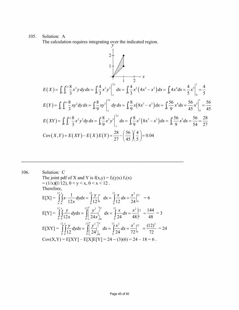
105. Solution: A The calculation requires integrating over the indicated region.
( ) ( )
( ) ( )
( ) ( )
2 11 2 1 1 12 2 2 2 2 2 4 5
0 0 0 00
2 11 2 1 1 12 3 3 3 4 5
0 0 0 00
21 2 12 2 2 3 2 3 3 5
0 0
8 4 4 4 44 43 3 3 5 5
8 8 8 56 56 5683 9 9 9 45 45
8 8 8 5683 9 9 9
xx
xx
xx
xx
xx
xx
E X x y dy dx x y dx x x x dx x dx x
E Y xy dy dx xy dy dx x x x dx x dx x
E XY x y dy dx x y dx x x x dx x d
= = = − = = =
= = = − = = =
= = = − =
∫ ∫ ∫ ∫ ∫
∫ ∫ ∫ ∫ ∫
∫ ∫ ∫
( ) ( ) ( ) ( )
1 1
0 0
56 2854 27
28 56 4Cov , 0.0427 45 5
x
X Y E XY E X E Y
= =
⎛ ⎞⎛ ⎞= − = − =⎜ ⎟⎜ ⎟⎝ ⎠⎝ ⎠
∫ ∫
-------------------------------------------------------------------------------------------------------- 106. Solution: C
The joint pdf of X and Y is f(x,y) = f2(y|x) f1(x) = (1/x)(1/12), 0 < y < x, 0 < x < 12 . Therefore,
E[X] = 12 12 12 2 12
0 00 0 0 0
112 12 12 24
x xy x xx dydx dx dxx
⋅ = = =∫ ∫ ∫ ∫ = 6
E[Y] = 12 12 122 2 12
00 0 0 00
14412 24 24 48 48
xx y y x xdydx dx dxx x
⎡ ⎤= = = =⎢ ⎥
⎣ ⎦∫ ∫ ∫ ∫ = 3
E[XY] = 12 12 122 2 3 312
00 0 0 00
(12)12 24 24 72 72
xx y y x xdydx dx dx⎡ ⎤
= = = =⎢ ⎥⎣ ⎦
∫ ∫ ∫ ∫ = 24
Cov(X,Y) = E[XY] – E[X]E[Y] = 24 − (3)(6) = 24 – 18 = 6 .
107. Solution: A
( ) ( )( ) ( ) ( ) ( )
( ) ( )( )
( ) ( )( )( )
1 2
22 2
2
Cov , Cov , 1.2
Cov , Cov , Cov ,1.2 Cov Y,1.2Y
Var Cov , 1.2Cov , 1.2Var
Var 2.2Cov , 1.2Var
Var 27.4 5 2.4
Var
C C X Y X Y
X X Y X X Y
X X Y X Y Y
X X Y Y
X E X E X
Y E Y
= + +
= + + +
= + + +
= + +
= − = − =
= ( )( )( ) ( )
( ) ( )( ) ( )
( ) ( ) ( )
2 2
1 2
51.4 7 2.4
Var Var Var 2Cov ,1 1 Cov , Var Var Var 8 2.4 2.4 1.62 2
Cov , 2.4 2.2 1.6 1.2 2.4 8.8
E Y
X Y X Y X Y
X Y X Y X Y
C C
− = − =
+ = + +
= + − − = − − =
= + + =
-------------------------------------------------------------------------------------------------------- 107. Alternate solution:
We are given the following information:
[ ]
[ ]
[ ]
1
2
2
2
1.25
27.4
7
51.4
Var 8
C X YC X YE X
E X
E Y
E Y
X Y
= += +
=
⎡ ⎤ =⎣ ⎦=
⎡ ⎤ =⎣ ⎦+ =
Now we want to calculate ( ) ( )
( )( ) [ ] [ ][ ] [ ]( ) [ ] [ ]( )
[ ] ( ) ( )( )
1 2
2 2
2 2
Cov , Cov , 1.2
1.2 1.2
2.2 1.2 1.2
2.2 1.2 5 7 5 1.2 7
27.
C C X Y X Y
E X Y X Y E X Y E X Y
E X XY Y E X E Y E X E Y
E X E XY E Y
= + +
= + + − + +⎡ ⎤⎣ ⎦⎡ ⎤= + + − + +⎣ ⎦⎡ ⎤ ⎡ ⎤= + + − + +⎣ ⎦ ⎣ ⎦
=
i
[ ] ( ) ( )( )[ ]
4 2.2 1.2 51.4 12 13.4
2.2 71.72
E XY
E XY
+ + −
= −
Therefore, we need to calculate [ ]E XY first. To this end, observe
[ ] ( ) [ ]( )[ ] [ ]( )
[ ] ( )[ ]
[ ][ ]
22
22 2
22 2
8 Var
2
2 5 7
27.4 2 51.4 144
2 65.2
X Y E X Y E X Y
E X XY Y E X E Y
E X E XY E Y
E XY
E XY
E XY
⎡ ⎤= + = + − +⎣ ⎦
⎡ ⎤= + + − +⎣ ⎦
⎡ ⎤ ⎡ ⎤= + + − +⎣ ⎦ ⎣ ⎦= + + −
= −
( )8 65.2 2 36.6= + =
Finally, ( ) ( )1, 2Cov 2.2 36.6 71.72 8.8C C = − = -------------------------------------------------------------------------------------------------------- 108. Solution: A The joint density of 1 2and T T is given by
( ) 1 21 2 1 2, , 0 , 0t tf t t e e t t− −= > >
Therefore, [ ] [ ]
( ) ( )
221 2 2 1
2 22 2
22
1 2
1122
1 2 20 0 00
1 1 1 12 2 2 2
2 20 0
1 1 1 1 12 2 2 2 2
0
Pr Pr 2
1
2 2 1 2
1 2
x tx x t xt t t t
x t x tx xt t
x t x x xt x x
x
X x T T x
e e dt dt e e dt
e e dt e e e dt
e e e e e e e
e
−− − − − −
− + − −− −
− − − − −− −
−
≤ = + ≤
⎡ ⎤= = −⎢ ⎥
⎢ ⎥⎣ ⎦⎡ ⎤ ⎛ ⎞
= − = −⎜ ⎟⎢ ⎥⎣ ⎦ ⎝ ⎠
⎡ ⎤= − + = − + + −⎢ ⎥⎣ ⎦
= − +
∫ ∫ ∫
∫ ∫
1 12 22 1 2 , 0
x xx xe e e e x− −− −− = − + >
It follows that the density of X is given by
( ) 1 12 21 2 , 0
x xx xdg x e e e e xdx
− −− −⎡ ⎤= − + = − >⎢ ⎥
⎣ ⎦
109. Solution: B
Let u be annual claims, v be annual premiums, g(u, v) be the joint density function of U and V, f(x) be the density function of X, and F(x) be the distribution function of X.
Then since U and V are independent,
( ) ( ) / 2 / 21 1, , 0 , 02 2
u v u vg u v e e e e u v− − − −⎛ ⎞= = ∞ ∞⎜ ⎟⎝ ⎠
< < < <
and
( ) [ ] [ ]
( )
( )
( )
/ 2
0 0 0 0
/ 2 / 2 / 200 0
1/ 2 / 2
0
1/ 2
Pr Pr Pr
1 ,2
1 1 1 2 2 21 1 2 2
1 2 1
vx vx u v
u v vx vx v v
v x v
v x v
uF x X x x U Vxv
g u v dudv e e dudv
e e dv e e e dv
e e dv
e ex
∞ ∞ − −
∞ ∞− − − − −
∞ − + −
− + −
⎡ ⎤= ≤ = ≤ = ≤⎢ ⎥⎣ ⎦
= =
⎛ ⎞= − = − +⎜ ⎟⎝ ⎠
⎛ ⎞= − +⎜ ⎟⎝ ⎠
= −+
∫ ∫ ∫ ∫
∫ ∫
∫
|
/ 2
0
1 12 1x
∞⎡ ⎤ = − +⎢ ⎥ +⎣ ⎦
Finally, ( ) ( )( )2
2'2 1
f x F xx
= =+
-------------------------------------------------------------------------------------------------------- 110. Solution: C Note that the conditional density function
( )( )
1 3,1 2, 0 ,3 1 3 3x
f yf y x y
f⎛ ⎞
= = < <⎜ ⎟⎝ ⎠
( )2 32 3 2 3 2
0 0 0
1 1624 1 3 8 43 9xf y dy y dy y⎛ ⎞ = = = =⎜ ⎟
⎝ ⎠ ∫ ∫
It follows that ( )1 9 9 21 3, , 03 16 2 3
f y x f y y y⎛ ⎞= = = < <⎜ ⎟
⎝ ⎠
Consequently, 1 3
1 3 2
00
9 9 1Pr 1 32 4 4
Y X X y dy y⎡ < = ⎤ = = =⎣ ⎦ ∫
111. Solution: E ( )( )
( ) ( )( )
( )
3
1
4 1 2 1 3
3 2
11
3 331 2
1
2,Pr 1 3 2
22 12,
4 2 1 2
1 1 122 4 4
11 82Finally, Pr 1 3 2 11 9 9
4
x
x
f yY X dy
f
f y y y
f y dy y
y dyY X y
− − − −
∞∞− −
−
−
⎡ < < = ⎤ =⎣ ⎦
= =−
= = − =
⎡ < < = ⎤ = = − = − =⎣ ⎦
∫
∫
∫
-------------------------------------------------------------------------------------------------------- 112. Solution: D
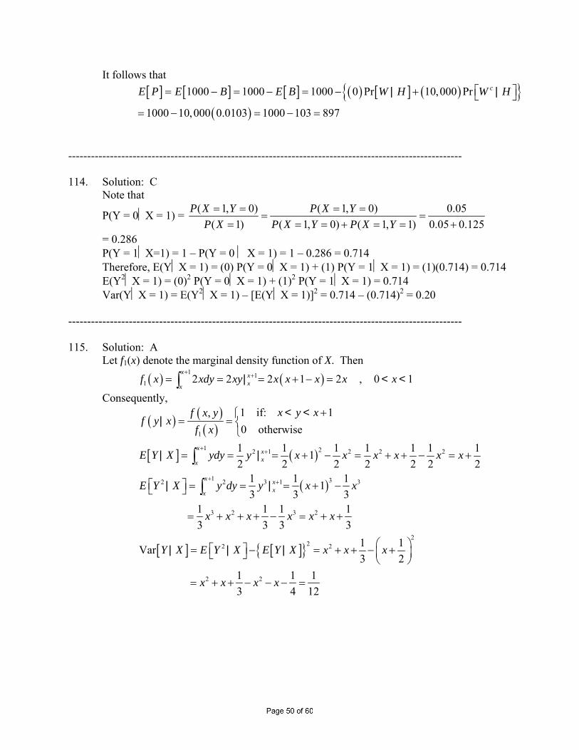
We are given that the joint pdf of X and Y is f(x,y) = 2(x+y), 0 < y < x < 1 .
Now fx(x) = 2
00
(2 2 ) 2x
xx y dy xy y⎡ ⎤+ = +⎣ ⎦∫ = 2x2 + x2 = 3x2, 0 < x < 1
so f(y|x) = 2 2
( , ) 2( ) 2 1( ) 3 3x
f x y x y yf x x x x
+ ⎛ ⎞= = +⎜ ⎟⎝ ⎠
, 0 < y < x
f(y|x = 0.10) = [ ]2 1 2 10 1003 0.1 0.01 3
y y⎡ ⎤+ = +⎢ ⎥⎣ ⎦, 0 < y < 0.10
P[Y < 0.05|X = 0.10] = [ ]0.05
0.052
00
2 20 100 1 1 510 1003 3 3 3 12 12
y dy y y⎡ ⎤+ = + = + =⎢ ⎥⎣ ⎦∫ = 0.4167 .
-------------------------------------------------------------------------------------------------------- 113. Solution: E
Let W = event that wife survives at least 10 years H = event that husband survives at least 10 years B = benefit paid P = profit from selling policies
Then [ ] [ ]Pr Pr 0.96 0.01 0.97cH P H W H W⎡ ⎤= ∩ + ∩ = + =⎣ ⎦ and
[ ] [ ][ ]
[ ]
Pr 0.96Pr 0.9897Pr 0.97
Pr 0.01Pr 0.0103Pr 0.97
cc
W HW H
H
H WW H
H
∩= = =
⎡ ⎤∩⎣ ⎦⎡ ⎤ = = =⎣ ⎦
|
|
It follows that [ ] [ ] [ ] ( ) [ ] ( ){ }
( )1000 1000 1000 0 Pr 10,000 Pr
1000 10,000 0.0103 1000 103 897
cE P E B E B W H W H⎡ ⎤= − = − = − + ⎣ ⎦= − = − =
| |
-------------------------------------------------------------------------------------------------------- 114. Solution: C
Note that
P(Y = 0⏐X = 1) = ( 1, 0) ( 1, 0) 0.05( 1) ( 1, 0) ( 1, 1) 0.05 0.125
P X Y P X YP X P X Y P X Y= = = =
= == = = + = = +
= 0.286 P(Y = 1⏐X=1) = 1 – P(Y = 0 ⏐ X = 1) = 1 – 0.286 = 0.714 Therefore, E(Y⏐X = 1) = (0) P(Y = 0⏐X = 1) + (1) P(Y = 1⏐X = 1) = (1)(0.714) = 0.714 E(Y2⏐X = 1) = (0)2 P(Y = 0⏐X = 1) + (1)2 P(Y = 1⏐X = 1) = 0.714 Var(Y⏐X = 1) = E(Y2⏐X = 1) – [E(Y⏐X = 1)]2 = 0.714 – (0.714)2 = 0.20
-------------------------------------------------------------------------------------------------------- 115. Solution: A
Let f1(x) denote the marginal density function of X. Then
( ) ( )1 1
1 2 2 2 1 2 , 0 1x x
xxf x xdy xy x x x x x
+ += = = + − =∫ | < <
Consequently,
( ) ( )( )
[ ] ( )
( )
[ ] [ ]{ }
1
1 22 1 2 2 2
1 32 2 3 1 3
3 2 3 2
22 2
1 if: 1,0 otherwise
1 1 1 1 1 1 112 2 2 2 2 2 2
1 1 113 3 3
1 1 1 1 3 3 3 3
Var
x xxx
x xxx
x y xf x yf y x
f x
E Y X ydy y x x x x x x
E Y X y dy y x x
x x x x x x
Y X E Y X E Y X x
+ +
+ +
+⎧= = ⎨
⎩
= = = + − = + + − = +
⎡ ⎤ = = = + −⎣ ⎦
= + + + − = + +
⎡ ⎤= − =⎣ ⎦
∫
∫
< <|
| |
| |
| | |2
2 2
1 13 2
1 1 1 3 4 12
x x
x x x x
⎛ ⎞+ + − +⎜ ⎟⎝ ⎠
= + + − − − =
116. Solution: D
Denote the number of tornadoes in counties P and Q by NP and NQ, respectively. Then E[NQ|NP = 0] = [(0)(0.12) + (1)(0.06) + (2)(0.05) + 3(0.02)] / [0.12 + 0.06 + 0.05 + 0.02] = 0.88 E[NQ
2|NP = 0] = [(0)2(0.12) + (1)2(0.06) + (2)2(0.05) + (3)2(0.02)] / [0.12 + 0.06 + 0.05 + 0.02] = 1.76 and Var[NQ|NP = 0] = E[NQ
2|NP = 0] – {E[NQ|NP = 0]}2 = 1.76 – (0.88)2 = 0.9856 .
-------------------------------------------------------------------------------------------------------- 117. Solution: C
The domain of X and Y is pictured below. The shaded region is the portion of the domain over which X<0.2 .
Now observe
[ ] ( )
( ) ( ) ( ) ( )
( ) ( ) ( )
10.2 1 0.2 2
0 0 00
0.2 0.22 2 2
0 0
0.2 2 3 30.200
1Pr 0.2 6 1 62
1 1 6 1 1 1 6 1 12 2
1 6 1 1 0.8 1 0.4882
xx
X x y dydx y xy y dx
x x x x dx x x dx
x dx x
−− ⎡ ⎤= − + = − −⎡ ⎤⎣ ⎦ ⎢ ⎥⎣ ⎦
⎡ ⎤ ⎡ ⎤= − − − − − = − − −⎢ ⎥ ⎢ ⎥⎣ ⎦ ⎣ ⎦
= − = − − = − + =
∫ ∫ ∫
∫ ∫
∫
<
|
-------------------------------------------------------------------------------------------------------- 118. Solution: E
The shaded portion of the graph below shows the region over which ( ),f x y is nonzero:
We can infer from the graph that the marginal density function of Y is given by
( ) ( ) ( )3 2 1 215 15 15 15 1 , 0 1y
y
yy
g y y dx xy y y y y y y= = = − = − < <∫
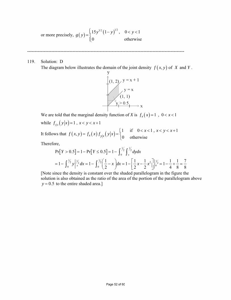
or more precisely, ( ) ( )1 23 215 1 , 0 10 otherwise
y y yg y⎧ − < <⎪= ⎨⎪⎩
-------------------------------------------------------------------------------------------------------- 119. Solution: D The diagram below illustrates the domain of the joint density ( ), of andf x y X Y .
We are told that the marginal density function of X is ( ) 1 , 0 1xf x x= < <
while ( ) 1 , 1y xf y x x y x= < < +
It follows that ( ) ( ) ( ) 1 if 0 1 , 1,
0 otherwisex y xx x y x
f x y f x f y x< < < < +⎧
= = ⎨⎩
Therefore,
[ ] [ ]1 1
2 2
0
1 11 12 2 22 200 0
Pr 0.5 1 Pr 0.5 1
1 1 1 1 1 71 1 1 12 2 2 4 8 8
x
x
Y Y dydx
y dx x dx x x
> = − ≤ = −
⎛ ⎞ ⎡ ⎤= − = − − = − − = − + =⎜ ⎟ ⎢ ⎥⎝ ⎠ ⎣ ⎦
∫ ∫
∫ ∫
[Note since the density is constant over the shaded parallelogram in the figure the solution is also obtained as the ratio of the area of the portion of the parallelogram above
0.5y = to the entire shaded area.]
120. Solution: A
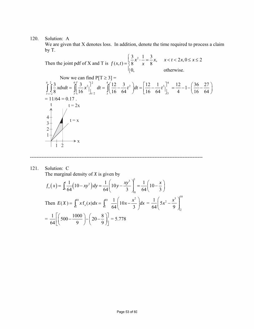
We are given that X denotes loss. In addition, denote the time required to process a claim by T.
Then the joint pdf of X and T is 23 1 3 , 2 ,0 2
( , ) 8 80, otherwise.
x x x t x xf x t x
⎧ ⋅ = < < ≤ ≤⎪= ⎨⎪⎩
Now we can find P[T ≥ 3] = 4 2 4 42 4
2 2 3
/ 2 33 / 2 3 3
3 3 12 3 12 1 12 36 2718 16 16 64 16 64 4 16 64tt
xdxdt x dt t dt t⎡ ⎤ ⎛ ⎞ ⎡ ⎤ ⎛ ⎞= = − = − = − − −⎜ ⎟ ⎜ ⎟⎢ ⎥ ⎢ ⎥⎣ ⎦ ⎝ ⎠ ⎣ ⎦ ⎝ ⎠∫ ∫ ∫ ∫
= 11/64 = 0.17 .
t
x1 2
3
4
1
2
t = x
t = 2x
-------------------------------------------------------------------------------------------------------- 121. Solution: C The marginal density of X is given by
( ) ( )131 2
00
1 1 110 10 1064 64 3 64 3x
xy xf x xy dy y⎛ ⎞ ⎛ ⎞= − = − = −⎜ ⎟ ⎜ ⎟
⎝ ⎠⎝ ⎠∫
Then 210 10
2 2
1( ) f ( ) 1064 3x
xE X x x dx x dx⎛ ⎞
= = −⎜ ⎟⎝ ⎠
∫ ∫ = 103
2
2
1 564 9
xx⎛ ⎞
−⎜ ⎟⎝ ⎠
= 1 1000 8500 2064 9 9
⎡ ⎤⎛ ⎞ ⎛ ⎞− − −⎜ ⎟ ⎜ ⎟⎢ ⎥⎝ ⎠ ⎝ ⎠⎣ ⎦ = 5.778
122. Solution: D
The marginal distribution of Y is given by f2(y) = 0
6y
∫ e–x e–2y dx = 6 e–2y 0
yxe−∫ dx
= −6 e–2y e–y + 6e–2y = 6 e–2y – 6 e–3y, 0 < y < ∞
Therefore, E(Y) = 0
y∞
∫ f2(y) dy = 2 3
0
(6 6 )y yye ye∞
− −−∫ dy = 6 2
0
yye∞
−∫ dy – 6 0
y∞
∫ e–3y dy =
0
6 22
∞
∫ ye–2y dy − 0
6 33
∞
∫ y e–3y dy
But 0
2∞
∫ y e–2y dy and 0
3∞
∫ y e–3y dy are equivalent to the means of exponential random
variables with parameters 1/2 and 1/3, respectively. In other words, 0
2∞
∫ y e–2y dy = 1/2
and 0
3∞
∫ y e–3y dy = 1/3 . We conclude that E(Y) = (6/2) (1/2) – (6/3) (1/3) = 3/2 – 2/3 =
9/6 − 4/6 = 5/6 = 0.83 . -------------------------------------------------------------------------------------------------------- 123. Solution: C Observe
[ ] [ ] [ ]
( ) ( )84 1 15 5 2
Pr 4 8 Pr 4 8 1 Pr 1 Pr 4 8 1 Pr 1
1 13 60.122
S S N N S N N
e e e e−− − −
< < = ⎡ < < = ⎤ = + ⎡ < < > ⎤ >⎣ ⎦ ⎣ ⎦
= − + −
=
*
*Uses that if X has an exponential distribution with mean μ
( ) ( ) ( ) 1 1Pr Pr Prba
t t
a b
a X b X a X b e dt e dt e eμμ μ μ
μ μ
−∞ ∞ −− −≤ ≤ = ≥ − ≥ = − = −∫ ∫
124. Solution: A
Because f(x,y) can be written as yx eeyfxf 22)()( −−= and the support of f(x,y) is a cross product, X and Y are independent. Thus, the condition on X can be ignored and it suffices to just consider yeyf 22)( −= .
Because of the memoryless property of the exponential distribution, the conditional density of Y is the same as the unconditional density of Y+3.
Because a location shift does not affect the variance, the conditional variance of Y is equal to the unconditional variance of Y.
Because the mean of Y is 0.5 and the variance of an exponential distribution is always equal to the square of its mean, the requested variance is 0.25.
--------------------------------------------------------------------------------------------------------------------- 125. Solution: E
The support of (X,Y) is 0 < y < x < 1.
2)()|(),(, == xfxyfyxf XYX on that support. It is clear geometrically (a flat joint density over the triangular region 0 < y < x < 1) that when Y = y
we have X ~ U(y, 1) so that 11
1)|( <<−
= xyfory
yxf .
By computation:
11
122
2)(
),()|(222)(
1 , <<−
=−
==⇒−== ∫ xyforyyyf
yxfyxfydxyf
yY
YXY
126. Solution: C
Using the notation of the problem, we know that 0 125
p p+ = and
0 1 2 3 4 5 1p p p p p p+ + + + + = . Let 1n np p c+− = for all 4n ≤ . Then 0 for 1 5np p nc n= − ≤ ≤ . Thus ( ) ( ) ( ) .115652 00000 =−=−++−+−+ cpcpcpcpp ...
Also ( )0 1 0 0 0225
p p p p c p c+ = + − = − = . Solving simultaneously 0
0
6 15 1225
p c
p c
− =⎧⎪⎨
− =⎪⎩
⇒
0
0
66 35
6 15 11125
p c
p c
c
− =
− + = −
=
. So 01 2 1 25 and 260 5 60 60
c p= = + = . Thus 025
120p = .
We want ( ) ( )4 5 0 017 15 324 5 0.267120 120 120
p p p c p c+ = − + − = + = = .
-----------------------------------------------------------------------------------------------------------
127. Solution: D
Because the number of payouts (including payouts of zero when the loss is below the deductible) is large, we can apply the central limit theorem and assume the total payout S is normal. For one loss there is no payout with probability 0.25 and otherwise the payout is U(0, 15000). So,
56257500*75.00*25.0][ =+=XE ,
000,250,56)12
150007500(*75.00*25.0][2
22 =++=XE , so the variance of one claim is
375,609,24][][)( 22 =−= XEXEXVar . Applying the CLT,
⎥⎥⎦
⎤
⎢⎢⎣
⎡<
−<−=<< 069044968.1
)375,609,24)(200()5625)(200(781741613.1]000,200,1000,000,1[ SPSP
which interpolates to 0.8575-(1-0.9626)=0.8201 from the provided table.
128. Key: B
Let H be the percentage of clients with homeowners insurance and R be the percentage of clients with renters insurance.
Because 36% of clients do not have auto insurance and none have both homeowners and renters insurance, we calculate that 8% (36% – 17% – 11%) must have renters insurance, but not auto insurance.
(H – 11)% have both homeowners and auto insurance, (R – 8)% have both renters and auto insurance, and none have both homeowners and renters insurance, so (H + R – 19)% must equal 35%. Because H = 2R, R must be 18%, which implies that 10% have both renters and auto insurance.
129. Key: B
The reimbursement is positive if health care costs are greater than 20, and because of the memoryless property of the exponential distribution, the conditional distribution of health care costs greater than 20 is the same as the unconditional distribution of health care costs.
We observe that a reimbursement of 115 corresponds to health care costs of 150 (100% x (120 – 20) + 50% x (150 – 120)), which is 130 greater than the deductible of 20.
Therefore,130100(115) (130) 1 0.727G F e
−= = − = .
130. Key: C
( )[ ] ( )[ ] ( )[ ] ( ) 9.415.0ln21
11005.0ln1001005.01005.0100 5.0ln =−
==== XXXX MeEEE
131. Solution: E
First, find the conditional probability function of 2N given 11 nN = : ( ) ( )( )11
21121|2
,|npnnp
nnp = ,
where ( )11 np is the marginal probability function of 1N . To find the latter, sum the joint probability function over all possible values of 2N obtaining
( ) ( ) ( )1
1
11
12111
1
2
211
1
241
431
41
43,
−∞
=
−−−−∞
=⎟⎠⎞
⎜⎝⎛=−⎟
⎠⎞
⎜⎝⎛== ∑∑
n
n
nnnn
n
eennpnp ,
since ( ) 111
1
2
211 =−∑∞
=
−−−
n
nnn ee as the sum of the probabilities of a geometric random variable. The
conditional probability function is
( ) ( )( ) ( ) 1
11
21121|2
211 1,|−−− −==
nnn eenpnnp
nnp ,
which is the probability function of a geometric random variable with parameter 1nep −= . The mean of this distribution is 11/1/1 nn eep == − , and becomes 2e when 21 =n . 132. Solution: C The number of defective modems is 20% x 30 + 8% x 50 = 10.
The probability that exactly two of a random sample of five are defective is 102.0
580
370
210
=
⎟⎟⎠
⎞⎜⎜⎝
⎛
⎟⎟⎠
⎞⎜⎜⎝
⎛⎟⎟⎠
⎞⎜⎜⎝
⎛
.
133. Solution: B Pr(man dies before age 50) = Pr(T < 50 | T > 40)
= )40(1
)40()50()40Pr(
)5040Pr(F
FFT
T−−
=><<
=
40 5040 50
40
1 1.1 1 1.1(1.1 1.1 )1000 1000
10001 1.1
1000
1e e ee
− −−
−
−= −
= 0.0696
Expected Benefit = 5000 Pr(man dies before age 50) = (5000) (0.0696) = 347.96

134. Solutions: C
Letting t denote the relative frequency with which twin-sized mattresses are sold, we have that the relative frequency with which king-sized mattresses are sold is 3t and the relative frequency with which queen-sized mattresses are sold is (3t+t)/4, or t. Thus, t = 0.2 since t + 3t + t = 1. The probability we seek is 3t + t = 0.80.
135. Key: E
Var (N) = E [ Var ( N | λ )] + Var [ E ( N | λ )] = E (λ) + Var (λ) = 1.50 + 0.75 = 2.25 136. Key: D
X follows a geometric distribution with 61
=p . Y = 2 implies the first roll is not a 6 and the
second roll is a 6. This means a 5 is obtained for the first time on the first roll (probability = 20%) or a 5 is obtained for the first time on the third or later roll (probability = 80%).
[ ] 826213| =+=+=≥p
XXE , so [ ] ( ) ( ) 6.688.012.02 =+==YXE
137. Key: E
Because X and Y are independent and identically distributed, the moment generating function of X + Y equals K2(t), where K(t) is the moment generating function common to X and Y. Thus, K(t) = 0.30e-t + 0.40 + 0.30et. This is the moment generating function of a discrete random variable that assumes the values -1, 0, and 1 with respective probabilities 0.30, 0.40, and 0.30. The value we seek is thus 0.70.