Elusive costs of sovereign defaults

Inter-American Development Bank

Banco Interamericano de Desarrollo (BID) Research Department

Departamento de Investigación Working Paper #581

The Elusive Costs of Sovereign Defaults

by

Eduardo Levy-Yeyati*

Ugo Panizza**

* Universidad Torcuato di Tella and World Bank

** Inter-American Development Bank

November 2006

2

Cataloging-in-Publication data provided by the Inter-American Development Bank Felipe Herrera Library Levy Yeyati, Eduardo.

The elusive costs of sovereign defaults / by Eduardo Levy-Yeyati, Ugo Panizza. p. cm. (Research Department Working paper series ; 581) Includes bibliographical references. 1. Finance, Public. 2. Default (Finance). 3. Debts, Public. I. Panizza, Ugo. II. Inter-

American Development Bank. Research Dept. III. Title. IV. Series.

HJ141 .L39 2006 336 L39-----dc22 ©2006 Inter-American Development Bank 1300 New York Avenue, N.W. Washington, DC 20577 The views and interpretations in this document are those of the authors and should not be attributed to the Inter-American Development Bank, or to any individual acting on its behalf. This paper may be freely reproduced provided credit is given to the Research Department, Inter-American Development Bank. The Research Department (RES) produces a quarterly newsletter, IDEA (Ideas for Development in the Americas), as well as working papers and books on diverse economic issues. To obtain a complete list of RES publications, and read or download them please visit our web site at: http://www.iadb.org/res.

3

Abstract*

Few would dispute that sovereign defaults entail significant economic costs, including, most notably, important output losses. However, most of the evidence supporting this conventional wisdom, based on annual observations, suffers from serious measurement and identification problems. To address these drawbacks, we examine the impact of default on growth by looking at quarterly data for emerging economies. We find that, contrary to what is typically assumed, output contractions precede defaults. Moreover, we find that the trough of the contraction coincides with the quarter of default, and that output starts to grow thereafter, indicating that default episode seems to mark the beginning of the economic recovery rather than a further decline. This suggests that, whatever negative effects a default may have on output, those effects result from anticipation of a default rather than the default itself.

* We would like to thank Eduardo Cavallo and other participants in the December 2005 IPES pre-conference, and we wish to thank Mariano Alvarez for excellent research assistance. The views expressed in this paper are the authors’ and do not necessarily reflect those of the Inter-American Development Bank.

4

“Hell, the last thing I should be doing is tell a country we should give up our claims. But there comes a time when you have to face reality.” “The problem historically has not been that countries have been to eager to renege on their financial obligations, but often too reluctant.1”

1. Introduction As conventional wisdom has it, a sovereign’s unilateral decision to stop servicing its debt carries

important and persistent economic costs. This is what is assumed (either explicitly or implicitly)

by the sovereign debt literature as a government’s main incentive to honor its obligations.2 In

this paper, we argue that using higher-frequency data yields a starkly different message. In

particular, we show that defaults have no significant negative impact on successive output

growth and, if anything, mark the final stage of the crisis and the beginning of economic

recovery.

The empirical literature has looked at the relationship between default and GDP growth

mainly in three ways: (i) output regressions directly controlling for default events; (ii) tests of the

effect of (current and past) defaults on access to the international credit market (more

specifically, borrowing costs); and (iii) tests of the effects on international trade (either due to the

drying up of trade credit or due to the implementation of trade sanctions). In all three cases, the

costs specifically associated with default (that is, in excess of those related to the ongoing crisis,

or to the memory of a recent crisis) are difficult to identify. While Ozler (1993) found that

defaults in the 1930s were associated with an increase in spreads of approximately 20 basis

points 40 years later, more recent work found that the effect of default on spreads is short-lived

(Ades et al., 2000; Borensztein and Panizza, 2005a). Focusing on the trade cost of defaults Rose

(2002) found that countries that defaulted on official (Paris Club) debt trade less with defaulted

1 The first quote is from an unnamed financial industry official; the second comes from a memo prepared by the Central Banks of England and Canada. Both are taken from Blustein (2005, pp. 163 and 102). 2 Sturzenegger (2004) finds a strong (albeit short-lived) negative contemporaneous effect on growth, and substantial output losses associated with defaults, a result confirmed by Borenzstein and Panizza (2005a). Both studies are based on annual observations.

5

countries, while Borensztein and Panizza (2005b) find that export-oriented industries tend to

suffer more in the aftermath of a default, though the effect is transitory.3

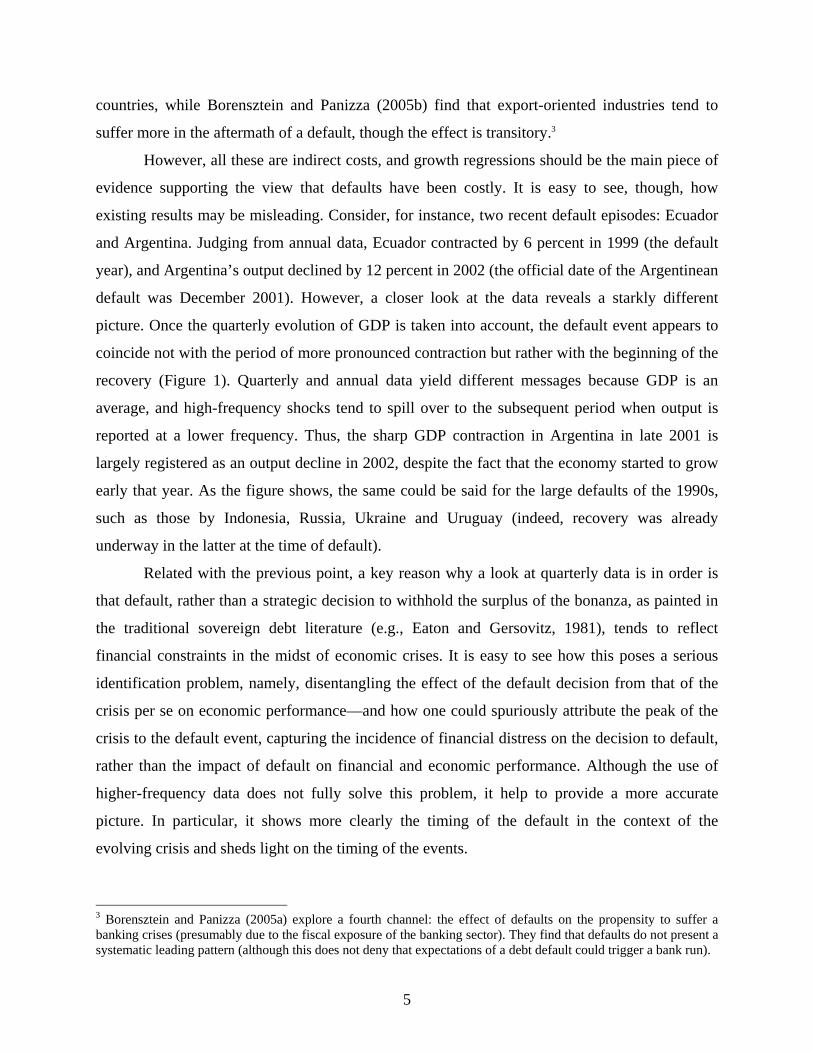
However, all these are indirect costs, and growth regressions should be the main piece of

evidence supporting the view that defaults have been costly. It is easy to see, though, how

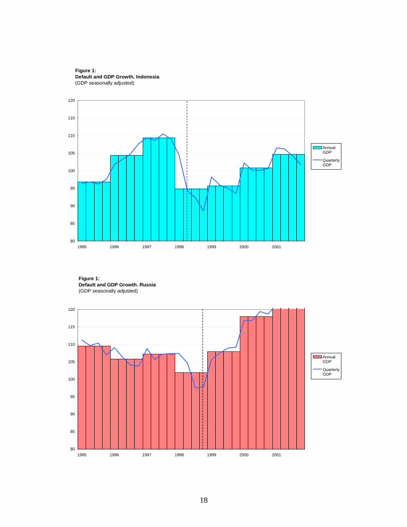
existing results may be misleading. Consider, for instance, two recent default episodes: Ecuador

and Argentina. Judging from annual data, Ecuador contracted by 6 percent in 1999 (the default

year), and Argentina’s output declined by 12 percent in 2002 (the official date of the Argentinean

default was December 2001). However, a closer look at the data reveals a starkly different

picture. Once the quarterly evolution of GDP is taken into account, the default event appears to

coincide not with the period of more pronounced contraction but rather with the beginning of the

recovery (Figure 1). Quarterly and annual data yield different messages because GDP is an

average, and high-frequency shocks tend to spill over to the subsequent period when output is

reported at a lower frequency. Thus, the sharp GDP contraction in Argentina in late 2001 is

largely registered as an output decline in 2002, despite the fact that the economy started to grow

early that year. As the figure shows, the same could be said for the large defaults of the 1990s,

such as those by Indonesia, Russia, Ukraine and Uruguay (indeed, recovery was already

underway in the latter at the time of default).

Related with the previous point, a key reason why a look at quarterly data is in order is

that default, rather than a strategic decision to withhold the surplus of the bonanza, as painted in

the traditional sovereign debt literature (e.g., Eaton and Gersovitz, 1981), tends to reflect

financial constraints in the midst of economic crises. It is easy to see how this poses a serious

identification problem, namely, disentangling the effect of the default decision from that of the

crisis per se on economic performance—and how one could spuriously attribute the peak of the

crisis to the default event, capturing the incidence of financial distress on the decision to default,

rather than the impact of default on financial and economic performance. Although the use of

higher-frequency data does not fully solve this problem, it help to provide a more accurate

picture. In particular, it shows more clearly the timing of the default in the context of the

evolving crisis and sheds light on the timing of the events.

3 Borensztein and Panizza (2005a) explore a fourth channel: the effect of defaults on the propensity to suffer a banking crises (presumably due to the fiscal exposure of the banking sector). They find that defaults do not present a systematic leading pattern (although this does not deny that expectations of a debt default could trigger a bank run).

6

With this in mind, in this paper we conduct a simple exercise: We replicate the standard

tests of the effect of default on growth and output using quarterly data for emerging economies.

The use of quarterly data allows us to date the default properly, to capture the evolution of output

more accurately, and to control for slowly moving fundamentals to better isolate the effect of

default.

We restrict our attention to a particular type of default, namely, default on debt with

private international investors. For this reason, we focus on emerging economies, which by

definition comprise globally integrated economies with a minimum volume of cross-border debt.

The emerging class provides a reasonably homogenous group exhibiting comparable external

vulnerability to capital account reversals (Sudden Stops) and, possibly, the highest propensity to

suffer from default episodes.4

Moving from yearly to quarterly data entails properly dating the default, which poses

non-trivial problems. Take, for instance, the recent events in Argentina. While Standard and

Poor’s gave a selective default rating in the last quarter of 2001 after a quasi-voluntary debt

exchange, most observers argue that a more accurate date of the default on international bonds is

January 2002, when the default was actually announced.5

In this paper, we compile a quarterly database on emerging market defaults and run panel

growth regressions controlling for crisis variables, both annual (to check consistency with

previous results reported in the literature) and quarterly. We include several leads and lags to

ensure that the results are not driven by dating errors. We find that, when we look at quarterly

data, growth rates in the post-default period are never significantly lower than in normal times.

Moreover, the evidence indicates that, contrary to what is typically assumed, the output

contractions often attributed to defaults actually precede them. Indeed, defaults mark the

inflection point at which output reaches its minimum and starts to recover.

This should not be interpreted as proof that defaults in general do not matter. On the

contrary, much in the way of a standard liquidity run, most of the financial distress that precedes

the default decision may be due to its anticipation. However, our findings have distinct

4 Extending this exercise to other countries is not straightforward. There are no recent defaults by industrial countries, and their inclusion as a control group is questionable. On the other hand, while there are defaults on debt with foreign banks in non-emerging, low income economies, availability of quarterly output data is in these case virtually null. 5 Importantly, Argentina had not missed a payment before that date. This example, however, shows that dating errors are only magnified when we look at annual data, yet another reason to go quarterly.

7

implications from a policy perspective. If defaults were costly a posteriori, the decision to default

should weigh these costs against the fiscal effort needed to service the debt. However, once the

default is anticipated (and its concomitant cost brought forward) by the market, the formal

decision to stop servicing the debt entails no tradeoff and is therefore optimal (and even

overdue).

The paper proceeds as follows. Section 2 describes the data, and Section 3 presents the

main empirical results. Finally, Section 4 discusses the implications of our findings for the

optimal timing of default and concludes.

Section 2. The Data Table 1 reports the summary statistics. Table A1 in the Appendix provides a definition of our

variables and the sources of data, and Table A2 lists all countries and periods covered in the

analysis.

Table 2 lists the default episodes in our sample. The tests below do not include all 23

default episodes listed in the table because some of them occurred within a relatively short

window and should be considered as spin-offs of the previous episode; their inclusion may bias

the results against finding a significant default cost. For this reason, we exclude default episodes

that happen within three years of the previous default (which leaves out the Indonesian defaults

of 2000 and 2002). Furthermore, we only include default on private lenders and hence exclude

the Pakistani default on Paris Club debt of 1997. As a consequence, our working sample includes

20 default episodes. Ten of these episodes took place in the 1980s and mostly concerned

international bank loans. The remaining 10 took place in the last 15 years and mostly involved

sovereign bonds.

First Impressions

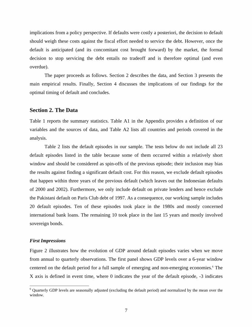
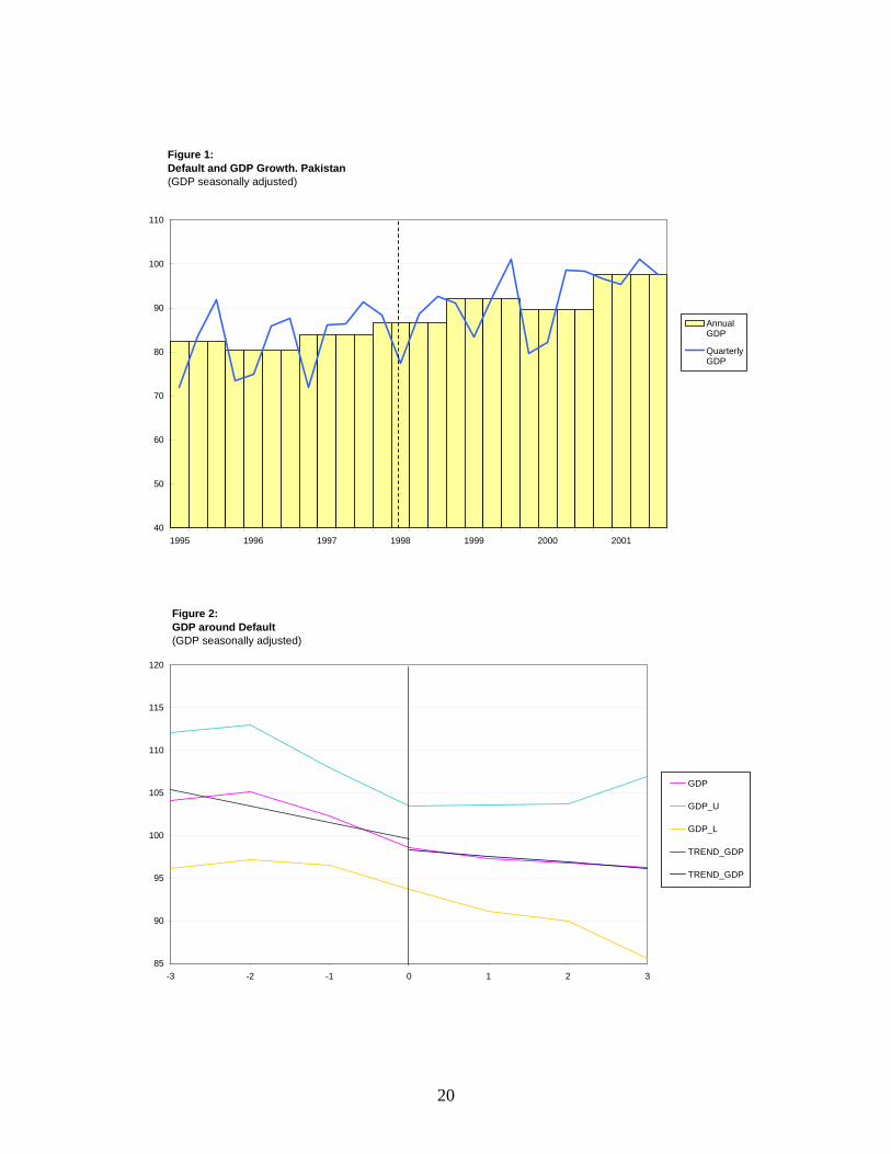
Figure 2 illustrates how the evolution of GDP around default episodes varies when we move

from annual to quarterly observations. The first panel shows GDP levels over a 6-year window

centered on the default period for a full sample of emerging and non-emerging economies.6 The

X axis is defined in event time, where 0 indicates the year of the default episode, -3 indicates

6 Quarterly GDP levels are seasonally adjusted (excluding the default period) and normalized by the mean over the window.

8

three years before the episode and 3 indicates three years after the event. This shows that GDP

starts decreasing two years before the event and keeps decreasing (albeit, at a slower rate) in the

following three years, a picture broadly consistent with the output cost of defaults identified in

panel growth regressions that use annual data.

In the second panel, we repeat the exercise for our emerging market sample. As before,

we see a clear drop in GDP in the three years before the default episode, whereas now the output

remains stable and close to its minimum in the following three years. Again, the declining trend

precedes the default event, but growth remains either negative or close to zero thereafter.

The third panel replicates the exercise once more, this time for the emerging market

sample and using quarterly data (now the X axis is measured in quarters). Now, we find a

slightly negative trend in the three years preceding the default episode combined with a steep

drop in the last three quarters of the pre-episode window. On the other hand, while GDP still

falls in the quarter after the event, the trend reverses immediately thereafter to a quick and steady

recovery to above pre-crisis levels. Thus, at least at this preliminary graphic level, going from

annual to quarterly data appears to change the message in a significant way.

3. Results Figure 2 provides suggestive evidence that the output costs of default are hard to find when

measured using quarterly data, but does not amount to a formal test. Such a test is reported in this

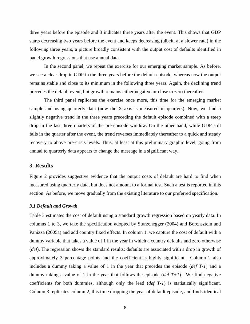
section. As before, we move gradually from the existing literature to our preferred specification. 3.1 Default and Growth Table 3 estimates the cost of default using a standard growth regression based on yearly data. In

columns 1 to 3, we take the specification adopted by Sturzenegger (2004) and Borensztein and

Panizza (2005a) and add country fixed effects. In column 1, we capture the cost of default with a

dummy variable that takes a value of 1 in the year in which a country defaults and zero otherwise

(def). The regression shows the standard results: defaults are associated with a drop in growth of

approximately 3 percentage points and the coefficient is highly significant. Column 2 also

includes a dummy taking a value of 1 in the year that precedes the episode (def T-1) and a

dummy taking a value of 1 in the year that follows the episode (def T+1). We find negative

coefficients for both dummies, although only the lead (def T-1) is statistically significant.

Column 3 replicates column 2, this time dropping the year of default episode, and finds identical

9

results. In columns 4 to 6, we run the same regressions without the control variables as an

intermediate step towards our quarterly specification, which excludes controls due to data

availability. Now def T+1 becomes statistically significant and large, indicating that growth in

the year after default is 2 percentage points lower than in tranquil times. Other than that, the

results are strikingly similar to the previous ones. The same applies to column 7 (where we

replicate the specification of column 4 for the sample of column 1), and to columns 8 to 10

(where we run similar regressions for our emerging market sample). Results are virtually

unchanged in all cases. In sum, based on annual data, during the three-year window around

default, growth rates appear to be significantly (and substantially) lower than average—although,

judging from the value of the coefficients, there is no indication that the decline accelerates after

the actual default event.

Reassured by the robustness of the previous results to sample and specification changes,

in Table 4 we repeat the exercise using quarterly GDP data. Column 1 includes only two

regressors: a dummy variable taking value 1 in the default quarter and a market pressure index

along the lines of Kaminsky and Reinhart (1999). The coefficient of the default dummy is

negative and very large, suggesting that at the time default materializes, (quarterly) growth is a

hefty 2.8 percent lower than in normal times. As expected, the market pressure variable is also

negative and statistically significant.7 Column 2 adds dummies for the quarters that precede and

follow the default event: unlike in the previous table, growth is now significantly lower in the

quarter before, but not in the quarter after default. The same message is delivered when we

include dummies for two and three periods before and after default (columns 3 and 4), and when

we use two dummies to indicate the corresponding leads and lags (columns 5 and 6). In

particular, growth is always significantly lower in the quarters leading to default but not in the

quarters following default (we report the joint test of leads and lags at the bottom panel of the

table).

Thus, a simple comparison of Tables 3 and 4 suggests that default materializes when the

crisis are already underway: the negative link revealed by annual data simply captures the fact

that defaults tend to occur in the context (and often as a result) of a crisis.

7 Dropping this variable or including a variable measuring changes in the real exchange rate does not affect our results.

10

Quarterly data may be more sensitive to (autocorrelated) measurement error that tends to

be corrected over time. However, the results are unaltered when we re-run the regressions

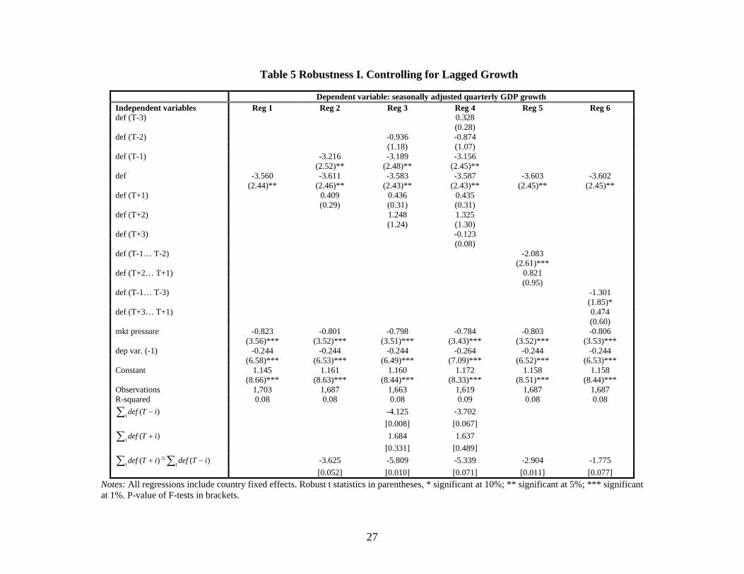
including the lagged dependent variable (Table 5). In turn, in Table 6, we control for country-

year fixed effects to capture the evolution of country-specific fundamentals at an annual

frequency. As such, this test encompasses all annual variables typically used in standard

specifications, including a crisis year dummy. The fact that the coefficients are never statistically

significant provides further indication that, once the crisis is controlled for, default does not exert

any visible influence on output.8

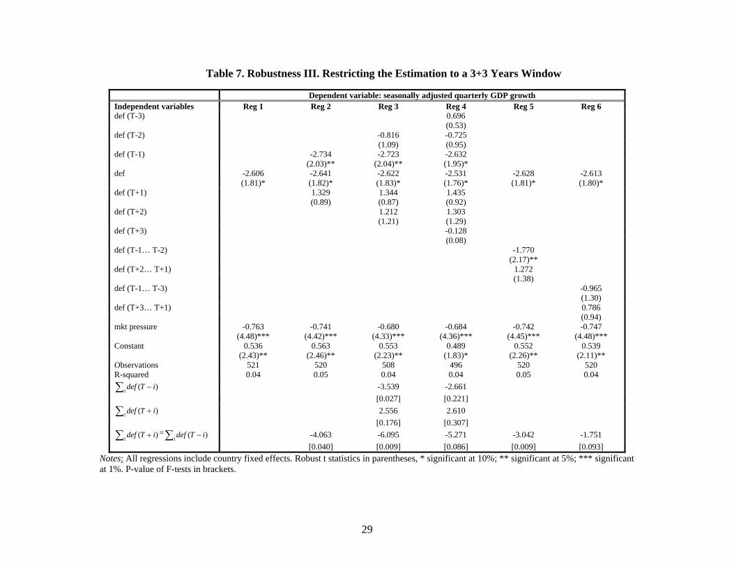
Table 7 explores the pre- and post-default periods in more detail by narrowing the

estimation window to six-year period centered around the default event. The results are again

unchanged. Table 8, in turn, explores the role of outliers (of particular relevance given the

relatively small number of events in our sample) by running the regression of Table 4, column 2

dropping one country at a time. The table, which highlights extreme values for the coefficients

and t-statistics, shows that the contemporaneous effect ranges between –1.79 and –2.88 and that

it is always statistically significant. The effect at T-1 ranges between –2.17 and –3.53 and is

statistically significant in 13 out of 14 regressions (when we exclude Peru, the p-value is 0.12).

By contrast, the effect at T+1 ranges between –0.27 and –1.79 and it is never statistically

significant (we obtain the lowest p value, 0.14, when we exclude Pakistan). Again, leads (but not

lags) help explain the evolution of output.

Table 9 presents a different look at the evidence that tests the intuition provided by

Figure 1: defaults mark the start of the recovery. To do that, we run an event-study like test that

compares cumulative growth rate before and after the default event for different windows

centered on the default quarter (which is dropped for the purposes of this computation).9 In this

way, we want to confirm not only that output trend declines before the actual default takes place,

but also that the declining trend is attenuated and even reverts after default. The results strongly

support this hypothesis: cumulative growth goes from negative to positive, and the difference

between growth rates before and after increases (Figure 3) to become significant as the window

widens. Default represents, rather than a trigger, the turning point of the crisis, possibly due to

8 The coefficients should be interpreted here as the deviation form the average growth rate in the year of default, and not as the deviation from the average growth rate in normal times. 9 Specifically, setting t = 0 for the default quarter, DGDP(-s) = [GDP(-1)/GDP(-s)]-1, and DGDP(+s) = [GDP(s)/GDP(+1)]-1.

11

non-trivial costs of avoiding default and to the fact that most of the consequences of default are

typically reflected in the markets before the decision is made official.

3.2 Growth-Inducing Defaults? The finding that defaults have been followed by periods of economic recovery should not be

mistaken as prima facie evidence of causality—much in the same way as the correlation between

default and annual growth should not be mistaken as saying that defaults are costly. A simple

inspection of Figure 1 suggests that, to the extent that larger recessions are followed by steeper

recoveries, the benign post-default outcome may be simply reflecting the association of defaults

with particularly deep economic downturns.

Indeed, Beaudry and Koop (1993) have shown that output expansions depend positively

on the “current depth of recession” (CDR), defined as the gap between current level of output

and its historical maximum. More generally, a growing body of literature has highlighted the

nonlinear nature of the business cycle and, in particular, the fact that growth rates depend

positively on the depth of the current output gap.10

We examine whether this argument can explain the finding of “growth-inducing defaults”

in two steps. First, we document that defaults are indeed associated with larger than average

recessions (note that so far, we have only documented an association between recessions and

defaults—more precisely, that the latter are typically preceded by the former—but not that the

fact that recessions are more pronounced prior to default events). Second, we rerun the baseline

regressions of Table 4 controlling for the current depth of the recession, captured by Beaudry and

Koop’s (1993) CDR variable, to see whether the link between defaults and growth is due to the

omission of the recession depth variable.

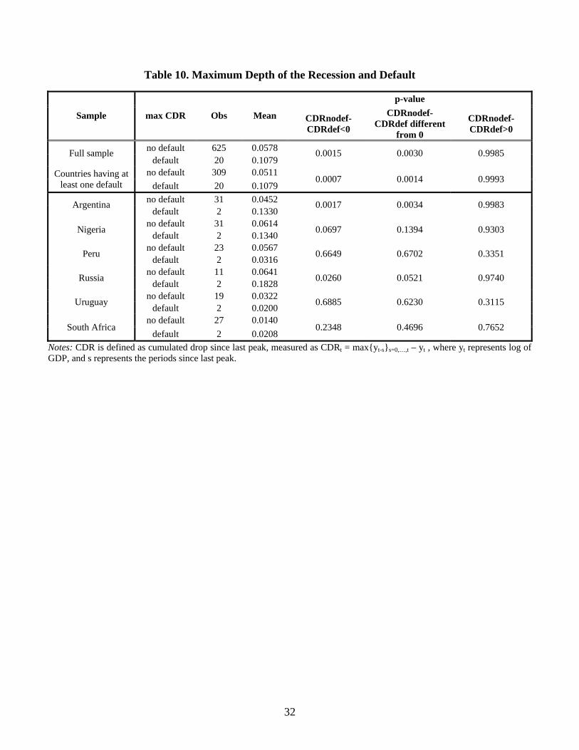
Table 10 reports the results from the first step, showing that the depth of the recession is

significantly larger for recessions leading to debt defaults. In the table, we first compare the

maximum recession depth in the absence of default for the whole sample, with the maximum

CDR reached in recessions that coincided with default events. As the means test indicates,

recessions are a significant 3 percent deeper during default episodes. The difference is even

larger when we restrict attention to countries that defaulted at least once in the period under

10 The underlying assumption is that, because of the excess capacity during the contractionary phase of the cycle, positive real shocks will have more persistent effects than negative shocks. See also Hamilton (1989), Jansen and Oh (1999), and Neftci (2001).

12

study: for defaulters, recessions have been nearly twice as deep when they ended in default than

otherwise. The same conclusion can be reached by looking at defaulters individually: pre-default

recessions are always deeper (and often significantly so).

Table 11, in turn, replicates the baseline regressions of Table 4, including the CDR

variable to test whether the expansionary effect of defaults can be attributed to the larger depth of

the preceding recessions. As expected, we find that CDR has a positive and statistical significant

effect on growth, which is robust to the inclusion of the lagged dependent variable (which

replicates Beaudry and Koop’s (1993) specification for the U.S.).11 More to the point of our test,

including the CDR variable does not alter our baseline result. First of all, we find that the leading

effect of the crisis remains virtually unaltered (negative and statistically significant). Second, we

find that including CDR and explicitly controlling for the effect of excess capacity somewhat

reduces the post-default recovery documented in Table 4 (for instance, the coefficient at def T+1

in Reg 2 goes from 1.1 to 0.4), but the coefficients for the post-default dummies remain positive

and insignificant. All this points out that our previous results were not driven by the fact that we

were not controlling for differences in the depth of the recession.

3.3 Default and Growth in the Long Run

Default may not have immediate effects on output, but may exert its influence over the long run,

either through lower investment or reduced access to capital markets.12 Because of that, the

analysis in this paper would not be complete without a look at the connection between default

episodes and the evolution of long run growth.

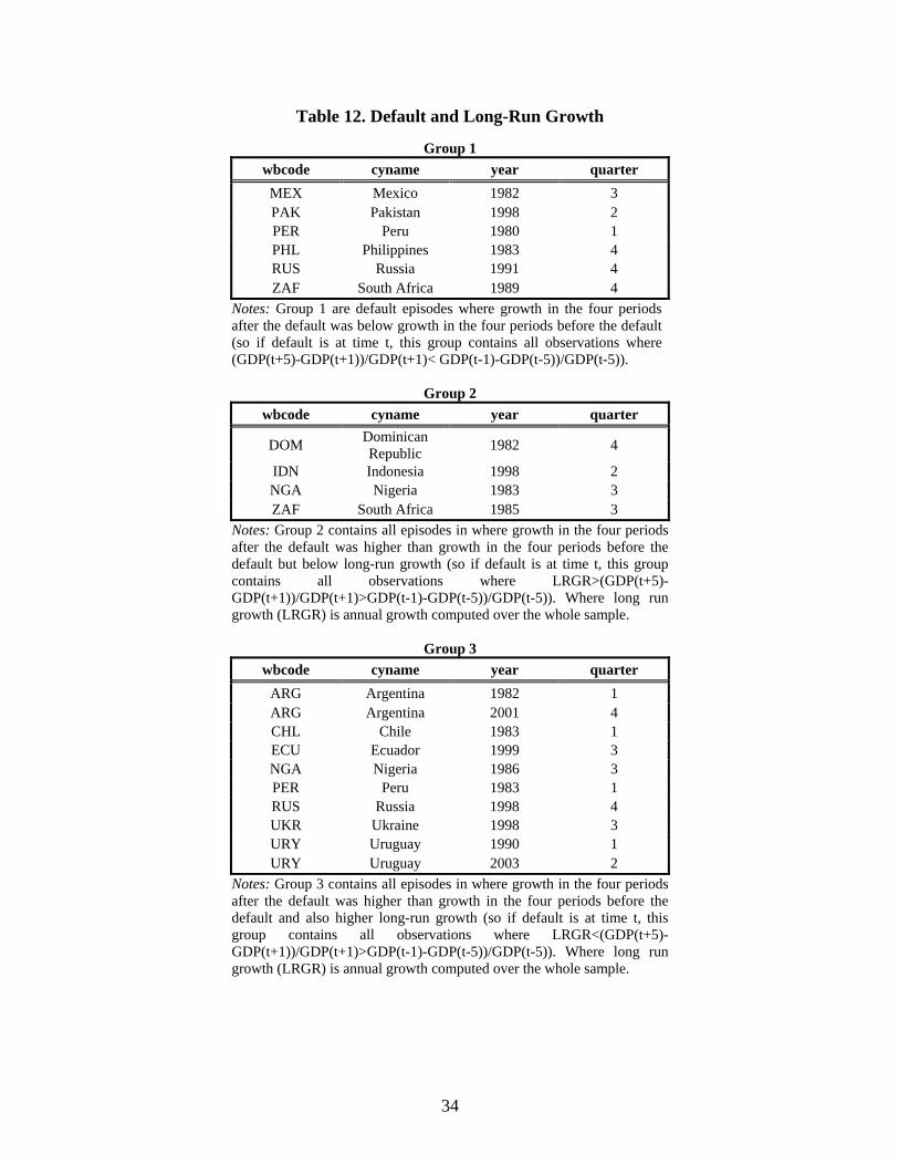
We look at this issue in two ways. First, we compare growth rates before and after the

event with the log linear trend growth. More precisely, we divide the defaults in our sample into

three groups, according to whether post-default growth was below pre-default growth, above pre-

default growth but below long-term growth, and above long-term growth. Table 12 reports the

result. As can be seen, whereas growth was stronger after default in 70 percent of the cases (in

line with our previous findings), it exceeded long-term growth in 50 percent of the cases,

suggesting that default, on average, does not deteriorate growth prospects.

11 Interestingly, the coefficient for our developing sample is roughly twice as large as the one found for the U.S., possibly as a combination of nonlinear output gap effects and deeper recessions. 12 While the evidence on the effect of default on access to finance as measured by its cost (specifically, the sovereign risk premium) is mixed at best (see Borenzstein and Panizza, 2005a), there is evidence that defaults may affect access through a reduced volume of funds (Levy Yeyati, 2006).

13

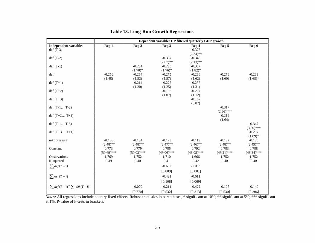
In Table 13, we look at the same issue from a different angle. Exploiting the variability of

HP-filtered long-term growth, we rerun the baseline regressions in Table 4, replacing the growth

rate with the long-term growth rate (computed country by country over the full sample period).

As can be seen, the decline in trend output that characterizes the period surrounding default

precedes the default event, and it does not appear to elicit an additional negative impact ex-post.

Thus, there seems to be no negative effect on the long-run output immediately after the default

event. Indeed, long-run growth appears to increase in the post-default period, as illustrated by

Figure 4, where we compare average HP-filtered output before and after the event. While the

difference in trends is not significant (as the one standard deviation intervals indicate), the figure

further confirms that defaults do not seem to exert a negative effect on output over the long run.

3.4 Default and Unemployment

Many observers would agree that, once income distribution is taken into account, unemployment

may be a more important—and persistent—determinant of social welfare than output growth

(Pernice and Sturzenegger, 2004). On the other hand, one would expect unemployment and real

growth to be closely correlated, so that the conclusions from the previous tests should extend to

this new variable. We show here that this is indeed the case.

Table 14 provides a preliminary look at the impact of sovereign defaults on

unemployment. The table replicates the specifications of Table 7 using unemployment instead of

real output growth as the dependent variable—that is, including the lagged dependent variable to

control for unemployment persistence. As before, we find that whatever negative influence

default may have on unemployment, it materializes before the actual default takes place. In

particular, the increase in unemployment in the run-up to default (with the highest increase

leading default by three quarters) reverts in the quarter of default.13

13 Most of the findings reported here for output growth are also obtained for the case of the unempoyment rate. Results are available upon request.

14

4. Conclusions This paper delivers a simple and sobering message: contrary to what it is typically presumed,

defaults have not been followed by output contractions. In fact, we find that the opposite seems

to be the case: the default quarter coincides with the trough of the output contraction and marks

the start of the economic recovery. This, however, does not appear to reflect a “benign” effect of

defaults but rather the fact that the latter are typically associated with particularly deep recessions

and, as a result, particularly steep recoveries.

This finding has important policy implications for debt management policies—and,

indirectly, for debt sustainability—that should be clarified. It does not imply that policies that

lead to default have no cost; on the contrary, the large GDP decline that typically precedes a

default may reflect in part the anticipation of the default decision. Indeed, it could be argued that,

if strategic defaults are costly, policymakers would only choose to default when these costs are

inevitable or have already been paid, hence the absence of observed costs documented in this

paper.14

However, the findings that these costs are largely paid before the default decision is made

also suggests that policymakers’ effort to further postpone a default that has been widely

anticipated and priced in by the market may be misguided. More generally, the argument bears

the question about the optimal timing of default. If the default decision entails a tradeoff between

the burden of servicing the debt (which grows as the crisis deepens and rollover costs mount),

and the additional cost of default (which declines as the crisis takes its toll), is the absence of

observed costs documented here an indication that defaults are often deferred for too long? Are

politicians willing to have the economy make a suboptimal effort to avoid a default that has

larger political than welfare costs?15 Is this agency problem and the associated political cost the

ultimate reason why countries honor their debts? Certainly fruitful questions for future research.

14 The finding that virtually all defaults appear to be driven by an adverse external context rather than by opportunistic behavior in times of bonanza is consistent with this view. 15 Borensztein and Panizza (2005a) discuss this hypothesis.

15

References Ades, A. et al. 2000. “Introducing GS-ESS: A New Framework for Assessing Fair Value in

Emerging Markets Hard-Currency Debt.” New York, United States: Goldman Sachs.

www.goldmansachs.com.

Barro, R.J., and J-W. Lee. 2000. “Internatinal Data on Educational Attainment: Updates and

Implications.” CID Working Paper 42. Cambridge, United States: Harvard University,

Center for International Development.

Beers, D. 2004. “Sovereign Defaults Set to Fall Again in 2005.” New York, United States:

Standard and Poors.

Beaudry, P., and G. Koop. 1993. “Do Recessions Permanently Change Output?” Journal of

Monetary Economics 31: 149-63.

Blustein, P. 2005. And the Money Kept Rolling In (and Out). New York, United States: Public

Affairs.

Bodman, P.M., and M. Crosby. 1998. “The Australian Business Cycle: Joe Palooka or Dead Cat

Bounce.” Department of Economics Working Paper 586. Melbourne, Australia:

University of Melbourne.

Borensztein, E., and U. Panizza. 2005a. “The Cost of Default.” Washington, DC, United States:

Inter-American Development Bank, Research Department. Mimeographed document.

Borensztein, E. and U. Panizza (2005b), “Do Sovereign Defaults Hurt Exporters?” Washington,

DC, United States: Inter-American Development Bank, Research Department.

Mimeographed document.

Caprio, G., and D. Klingebiel. 2003. “Episodes of Systemic and Borderline Financial Crises.”

Washington, DC, United States: World Bank. http://econ.worldbank.org/

Eaton, J., and M. Gersovitz. 1981. “Debt with Potential Repudiation: Theoretical and Empirical

Analysis.” Review of Economic Studies 48(2): 289-309.

Global Development Finance. 2003. Analysis and Statistical Appendix. Washington, DC, United

States: World Bank.

Hamilton, J.D. 1989. “A New Approach to the Economic Analysis of Nonstationary Time Series

and the Business Cycle.” Econometrica 57: 357–84.

International Financial Statistics. Washington, DC, United States: International Monetary Fund.

www.imf.org.

16

Jansen, D., and W. Oh. 1999. “Modeling Nonlinearity of Business Cycles: Choosing between the

CDR and STAR Models.” Review of Economics and Statistics 81: 344-349.

Kaminsky, G., and C. Reinhart. 1999. “The Twin Crises: The Causes of Banking and Balance-

of-Payments Problems.” American Economic Review 89(3): 473-500.

Levy Yeyati, E. 2006. “Optimal Debt? On the Insurance Value of International Debt Flows to

Developing Countries.” Washington, DC, United States: Inter-American Development

Bank, Research Department. Mimeographed document.

Martínez, J.V., and G. Sandleris. 2004. “Is it Punishment? Sovereign Defaults and the Declines

in Trade.” New York, United States: Columbia University. Mimeographed document.

Neftci, S.N. 2001. “Are Economic Time Series Asymmetric over the Business Cycle?” Journal

of Political Economy 92: 307-28.

Ozler, S. 1993. “Have Commercial Banks Ignored History?” American Economic Review 83(3):

608-20.

Pernice, S., and F. Sturzenegger. 2004. “Culture and Social Resistance to Reform: A Theory

about the Endogeneity of Public Beliefs with an Application to the Case of Argentina.”

CEMA Working Paper 275. Buenos Aires, Argentina: CEMA University.

Rose, A. 2002. “One Reason Countries Pay Their Debts: Renegotiation and International Trade.”

NBER Working Paper 8853. Cambridge, United States: National Bureau of Economic

Research.

Sturzenegger, F. 2004. “Toolkit for the Analysis of Debt Problems.” Journal of Restructuring

Finance 1(1): 201-203.

17

Figures and Tables

Figure 1:Default and GDP Growth. Argentina(GDP seasonally adjusted)

80

85

90

95

100

105

110

115

120

1998 1999 2000 2001 2002 2003 2004

AnnualGDP

QuarterlyGDP

Figure 1: Default and GDP Growth. Ecuador(GDP seasonally adjusted)

80

85

90

95

100

105

110

115

120

1996 1997 1998 1999 2000 2001 2002

AnnualGDP

QuarterlyGDP

18

Figure 1:Default and GDP Growth. Indonesia(GDP seasonally adjusted)

80

85

90

95

100

105

110

115

120

1995 1996 1997 1998 1999 2000 2001

AnnualGDP

QuarterlyGDP

Figure 1:Default and GDP Growth. Russia(GDP seasonally adjusted)

80

85

90

95

100

105

110

115

120

1995 1996 1997 1998 1999 2000 2001

AnnualGDP

QuarterlyGDP

19

Figure 1: Default and GDP Growth. Ukraine(GDP seasonally adjusted)

80

85

90

95

100

105

110

115

120

1995 1996 1997 1998 1999 2000 2001

AnnualGDP

QuarterlyGDP

Figure 1:Default and GDP Growth. Uruguay(GDP seasonally adjusted)

60

70

80

90

100

110

120

2000 2001 2002 2003 2004

AnnualGDP

QuarterlyGDP

20

Figure 1:Default and GDP Growth. Pakistan(GDP seasonally adjusted)

40

50

60

70

80

90

100

110

1995 1996 1997 1998 1999 2000 2001

AnnualGDP

QuarterlyGDP

Figure 2: GDP around Default(GDP seasonally adjusted)

85

90

95

100

105

110

115

120

-3 -2 -1 0 1 2 3

GDP

GDP_U

GDP_L

TREND_GDP

TREND_GDP

21


85

90

95

100

105

110

115

120

-3 -2 -1 0 1 2 3

GDP

GDP_U

GDP_L

TREND_GDP

TREND_GDP


85

90

95

100

105

110

115

120

-12 -8 -4 0 4 8 12

GDP

GDP_U

GDP_L

TREND_GDP

TREND_GDP

22

Figure 3: Cumulative Output Growth before and after Default(growth of GDP seasonally adjusted)

-6

-4

-2

0

2

4

6

1 2 3 4 5 6

DGDP(+t)

DGDP(-t)

Figure 4: GDP around Default(HP filtered GDP)

85

90

95

100

105

110

115

120

-12 -8 -4 0 4 8 12

GDP

GDP_U

GDP_L

TREND_GDP

TREND_GDP

23

Table 1. Summary Statistics

A. Yearly Variables

Variable Obs Mean Std. Dev. Min Max growth 482 1.675 4.877 -14.568 11.190 invgdp 460 1.773 0.725 0.329 4.215 pop growth 523 1.540 1.019 -3.248 3.390 sec 415 21.889 10.841 3.800 52.400 pop level 523 45.085 43.462 3.060 212.000 gov 460 0.035 0.095 -0.256 0.700 civil 495 3.741 1.228 1.000 7.000 �tt 474 -0.010 0.158 -2.080 1.067 openness 484 0.299 0.168 0.052 1.146 bank2av1 533 0.167 0.373 0 1 def 533 0.043 0.203 0 1

B. Quarterly Variables

Variable Obs Mean Std. Dev. Min Max growth 2,326 0.723791 5.558707 -27.3833 29.99361 external 2,298 90.78833 22.97053 13.93941 200.5199 mkt pressure 1,808 0.015815 0.487086 -5.32106 13.66791

24

Table 2: Default Episodes Included in the Sample

Country Year Quarter Default 1982 1 Default on external bank loans

Argentina 2001 4 Default on external bonds/Default on external bank loans

Chile 1983 1 Default on external bank loans 1982 4 Default on external bank loans Dominican

Republic 1999 2 Default on domestic bonds Ecuador 1999 3 Default on external bonds

Indonesia 1998 2 Default on external bank loans Mexico 1982 3 Default on external bank loans

1983 3 Default on external bank loans Nigeria 1986 3 Default on external bonds 1997 3 Paris club default Pakistan 1998 2 Default on external bank loans 1980 1 Default on external bank loans Peru 1983 1 Default on external bank loans

Philippines 1983 4 Default on external bank loans

1991 4 Default on external bank loans 1998 3 Default on domestic bonds Russia 1998 4 Default on external bonds 1985 3 Default on external bank loans South

Africa 1989 4 Default on external bank loans

Ukraine 1998 3 Default on domestic bonds/Default on external bonds/Default on domestic bonds

1990 1 Default on external bank loans Uruguay 2003 2 Default on external bonds

25

Table 3. Growth regressions (yearly data) Dependent variable: yearly GDP growth Full sample Emerging economies Independent

variables Reg 1 Reg 2 Reg 3 Reg 4 Reg 5 Reg 6 Reg 71 Reg 8 Reg 9 Reg 10 Reg 112

invgdp 1.834 1.784 1.780 (7.18)*** (6.99)*** (6.95)*** pop growth -0.452 -0.444 -0.452 (3.10)*** (3.00)*** (3.07)*** sec -0.015 -0.018 -0.022 (0.99) (1.22) (1.47) pop level 0.003 0.003 0.003 (0.72) (0.78) (0.89) gov 3.161 3.201 3.086 (3.16)*** (3.20)*** (3.08)*** civil 0.027 0.028 0.029 (0.24) (0.25) (0.27) Δtt -0.331 -0.214 0.911 (0.28) (0.18) (1.93)* openness 5.809 5.993 6.797 (3.75)*** (3.87)*** (4.45)*** bank2av1 -0.979 -0.920 -0.948 (4.04)*** (3.81)*** (3.95)*** def (T-1) -2.638 -2.618 -3.013 -3.001 -3.297 -3.410 (3.76)*** (3.75)*** (5.34)*** (5.31)*** (2.43)** (2.54)** Def -3.010 -3.207 -3.549 -3.824 -3.343 -3.715 -3.051 -3.505 (3.45)*** (3.67)*** (6.56)*** (7.08)*** (3.98)*** (3.56)*** (3.15)*** (2.11)** def (T+1) -0.552 -0.458 -2.212 -2.188 -2.352 -2.348 (0.89) (0.73) (3.74)*** (3.64)*** (2.05)** (2.01)** Constant -2.179 -2.061 -2.236 1.604 1.689 1.697 1.724 2.080 2.118 1.814 1.828 (2.69)*** (2.53)** (2.74)*** (26.04)*** (27.11)*** (27.34)*** (21.14)*** (8.90)*** (9.20)*** (8.41)*** (7.37)***Observations 2,153 2,153 2,114 4,841 4,839 4,763 2,153 454 433 482 287 Countries 89 89 89 181 181 181 89 28 28 28 14 R-squared 0.10 0.11 0.10 0.01 0.02 0.01 0.10 0.05 0.03 0.02 0.03

Notes: All regressions include country fixed effects. Robust t statistics in parentheses, * significant at 10%; ** significant at 5%; *** significant at 1% 1 Same sample as in column (1). 2 Sample used in the quarterly regressions.

26

Table 4. Quarterly Data, Baseline Model

Dependent variable: seasonally adjusted quarterly GDP growth Independent variables Reg 1 Reg 2 Reg 3 Reg 4 Reg 5 Reg 6 def (T-3) 0.463 (0.37) def (T-2) -1.002 -0.954 (1.39) (1.31) def (T-1) -2.916 -2.900 -2.854 (2.17)** (2.17)** (2.11)** def -2.802 -2.833 -2.811 -2.763 -2.834 -2.835 (2.00)** (2.02)** (2.02)** (1.99)** (2.01)** (2.01)** def (T+1) 1.142 1.161 1.208 (0.80) (0.80) (0.83) def (T+2) 1.017 1.066 (1.01) (1.05) def (T+3) -0.369 (0.23) def (T-1… T-2) -1.970 (2.47)** def (T+2… T+1) 1.067 (1.21) def (T-1… T-3) -1.183 (1.65)* def (T+3… T+1) 0.562 (0.69) mkt pressure -0.833 -0.822 -0.776 -0.766 -0.821 -0.823 (3.98)*** (3.94)*** (3.85)*** (3.82)*** (3.94)*** (3.95)*** Constant 0.858 0.862 0.896 0.884 0.862 0.863 (6.48)*** (6.41)*** (6.53)*** (6.24)*** (6.33)*** (6.27)*** Observations 1,745 1,729 1,688 1,644 1,729 1,729 R-squared 0.01 0.02 0.02 0.02 0.02 0.02

∑ −1

)( iTdef -3.902 -3.345 [0.012] [0.105]

∑ +1

)( iTdef 2.178 1.905 [0.225] [0.437]

∑ +1

)( iTdef =∑ −1

)( iTdef -4.058 -6.080 -5.250 -3.037 -1.745 [0.036] [0.008] [0.084] [0.008] [0.091]

Notes: All regressions include country fixed effects. Robust t statistics in parentheses, * significant at 10%; ** significant at 5%; *** significant at 1%. P-value of F-tests in brackets.

27

Table 5 Robustness I. Controlling for Lagged Growth

Dependent variable: seasonally adjusted quarterly GDP growth Independent variables Reg 1 Reg 2 Reg 3 Reg 4 Reg 5 Reg 6 def (T-3) 0.328 (0.28) def (T-2) -0.936 -0.874 (1.18) (1.07) def (T-1) -3.216 -3.189 -3.156 (2.52)** (2.48)** (2.45)** def -3.560 -3.611 -3.583 -3.587 -3.603 -3.602 (2.44)** (2.46)** (2.43)** (2.43)** (2.45)** (2.45)** def (T+1) 0.409 0.436 0.435 (0.29) (0.31) (0.31) def (T+2) 1.248 1.325 (1.24) (1.30) def (T+3) -0.123 (0.08) def (T-1… T-2) -2.083 (2.61)*** def (T+2… T+1) 0.821 (0.95) def (T-1… T-3) -1.301 (1.85)* def (T+3… T+1) 0.474 (0.60) mkt pressure -0.823 -0.801 -0.798 -0.784 -0.803 -0.806 (3.56)*** (3.52)*** (3.51)*** (3.43)*** (3.52)*** (3.53)*** dep var. (-1) -0.244 -0.244 -0.244 -0.264 -0.244 -0.244 (6.58)*** (6.53)*** (6.49)*** (7.09)*** (6.52)*** (6.53)*** Constant 1.145 1.161 1.160 1.172 1.158 1.158 (8.66)*** (8.63)*** (8.44)*** (8.33)*** (8.51)*** (8.44)*** Observations 1,703 1,687 1,663 1,619 1,687 1,687 R-squared 0.08 0.08 0.08 0.09 0.08 0.08

∑ −1

)( iTdef -4.125 -3.702 [0.008] [0.067]

∑ +1

)( iTdef 1.684 1.637 [0.331] [0.489]

∑ +1

)( iTdef =∑ −1

)( iTdef -3.625 -5.809 -5.339 -2.904 -1.775 [0.052] [0.010] [0.071] [0.011] [0.077]


28

Table 6. Robustness II. Controlling for Country-Year Effects

Dependent variable: seasonally adjusted quarterly GDP growth Independent variables Reg 1 Reg 2 Reg 3 Reg 4 Reg 5 Reg 6 def (T-3) 1.681 (0.85) def (T-2) -0.136 0.637 (0.08) (0.29) def (T-1) -2.455 -2.204 -1.457 (1.74)* (1.28) (0.71) def -2.401 -2.805 -2.467 -1.797 -2.321 -1.643 (1.54) (1.70)* (1.27) (0.81) (1.20) (0.77) def (T+1) 1.388 1.869 2.228 (0.74) (0.93) (1.04) def (T+2) 1.611 1.789 (1.21) (1.26) def (T+3) -0.154 (0.08) def (T-1… T-2) -1.099 (0.73) def (T+2… T+1) 1.888 (1.45) def (T-1… T-3) 0.245 (0.14) def (T+3… T+1) 1.589 (1.27) mkt pressure -0.668 -0.660 -0.627 -0.627 -0.671 -0.677 (2.26)** (2.22)** (2.10)** (2.09)** (2.26)** (2.28)** Constant 0.852 0.853 0.867 0.821 0.828 0.791 (5.84)*** (5.77)*** (5.46)*** (4.64)*** (5.30)*** (4.70)*** Observations 1,745 1,729 1,688 1,644 1,729 1,729 R-squared 0.12 0.12 0.11 0.12 0.12 0.12

∑ −1

)( iTdef -2.340 0.861 [0.432] [0.875]

∑ +1

)( iTdef 3.480 3.863 [0.196] [0.344]

∑ +1

)( iTdef =∑ −1

)( iTdef -3.843 -5.820 -3.002 -2.987 -1.344 [0.079] [0.054] [0.545] [0.054] [0.392]


29

Table 7. Robustness III. Restricting the Estimation to a 3+3 Years Window

Dependent variable: seasonally adjusted quarterly GDP growth Independent variables Reg 1 Reg 2 Reg 3 Reg 4 Reg 5 Reg 6 def (T-3) 0.696 (0.53) def (T-2) -0.816 -0.725 (1.09) (0.95) def (T-1) -2.734 -2.723 -2.632 (2.03)** (2.04)** (1.95)* def -2.606 -2.641 -2.622 -2.531 -2.628 -2.613 (1.81)* (1.82)* (1.83)* (1.76)* (1.81)* (1.80)* def (T+1) 1.329 1.344 1.435 (0.89) (0.87) (0.92) def (T+2) 1.212 1.303 (1.21) (1.29) def (T+3) -0.128 (0.08) def (T-1… T-2) -1.770 (2.17)** def (T+2… T+1) 1.272 (1.38) def (T-1… T-3) -0.965 (1.30) def (T+3… T+1) 0.786 (0.94) mkt pressure -0.763 -0.741 -0.680 -0.684 -0.742 -0.747 (4.48)*** (4.42)*** (4.33)*** (4.36)*** (4.45)*** (4.48)*** Constant 0.536 0.563 0.553 0.489 0.552 0.539 (2.43)** (2.46)** (2.23)** (1.83)* (2.26)** (2.11)** Observations 521 520 508 496 520 520 R-squared 0.04 0.05 0.04 0.04 0.05 0.04

∑ −1

)( iTdef -3.539 -2.661 [0.027] [0.221]

∑ +1

)( iTdef 2.556 2.610 [0.176] [0.307]

∑ +1

)( iTdef =∑ −1

)( iTdef -4.063 -6.095 -5.271 -3.042 -1.751 [0.040] [0.009] [0.086] [0.009] [0.093]


30

Table 8. Robustness IV. Dropping One Country at a Time

Dropping Contemporaneous effect T+1 T-1 Coefficient |t-statistics| Coefficient |t-statistics| Coefficient |t-statistics| -2.37 2.18 -1.02 0.75 -3.09 2.13 Argentina -2.31 2.10 -0.34 0.23 -2.81 1.79 Chile -2.71 2.64 -1.22 0.83 -2.64 1.83 Dominican Republic -2.35 2.15 -1.21 0.82 -3.45 2.38 Ecuador -2.37 2.16 -1.02 0.68 -2.98 1.98 Indonesia -1.87 1.88 -0.86 0.58 -2.93 1.95 Mexico -2.37 2.16 -0.87 0.59 -2.96 1.97 Nigeria -2.01 1.78 -0.27 0.19 -3.53 2.67 Pakistan -1.79 1.92 -1.79 1.45 -3.04 2.03 Peru -2.55 2.23 -1.11 0.72 -2.17 1.57 Philippines -2.03 1.93 -1.49 1.07 -2.80 1.88 Russia -2.77 2.50 -0.89 0.66 -3.23 2.10 South Africa -2.41 2.08 -1.16 0.74 -3.23 2.03 Ukraine -2.30 2.10 -0.75 0.51 -3.52 2.47 Uruguay -2.88 2.65 -0.83 0.53 -3.51 2.30 Notes: Specification (2) of Table 4.

31

Table 9. Cumulative Output Growth before and after Default

Change in Growth Obs Mean DGP(-T)-DGP(+T) p-value DGP(-T)-DGP(+T)<0

DGDP(-2) 14 -1.35 DGDP(+2) 14 1.36

-2.71 0.0766

DGDP(-3) 14 -2.77 DGDP(+3) 14 0.38

-3.15 0.0797

DGDP(-4) 13 -1.69 DGDP(+4) 14 -0.06

-1.63 0.2804

DGDP(-5) 12 -2.41 DGDP(+5) 14 1.71

-4.13 0.0997

DGDP(-6) 12 -4.69 DGDP(+6) 13 5.36

-10.04 0.0037

Notes: The table reports and compares the average cumulative growth rate before and after the default event, for windows of increasing length. For a window of length 2T+1, we drop the default quarter t = 0, and compute DGDP(-s) = [GDP-1/GDP-s]-1, and DGDP(+s) = [GDP+s/GDP+1]-1.

32

Table 10. Maximum Depth of the Recession and Default

p-value

Sample max CDR Obs Mean CDRnodef-CDRdef<0

CDRnodef-CDRdef different

from 0

CDRnodef-CDRdef>0

no default 625 0.0578 Full sample default 20 0.1079

0.0015 0.0030 0.9985

no default 309 0.0511 Countries having at least one default default 20 0.1079

0.0007 0.0014 0.9993

no default 31 0.0452 Argentina default 2 0.1330

0.0017 0.0034 0.9983

no default 31 0.0614 Nigeria default 2 0.1340 0.0697 0.1394 0.9303

no default 23 0.0567 Peru default 2 0.0316 0.6649 0.6702 0.3351

no default 11 0.0641 Russia default 2 0.1828 0.0260 0.0521 0.9740

no default 19 0.0322 Uruguay default 2 0.0200 0.6885 0.6230 0.3115

no default 27 0.0140 South Africa

default 2 0.0208 0.2348 0.4696 0.7652

Notes: CDR is defined as cumulated drop since last peak, measured as CDRt = max{yt-s}s=0,…,t – yt , where yt represents log of GDP, and s represents the periods since last peak.

33

Table 11. Current Depth of the Recession and Growth after Default

Dependent variable: seasonally adjusted quarterly GDP growth Independent variables Reg 1 Reg 2 Reg 3 Reg 4 Reg 5 Reg 6 def (T-3) 0.253 (0.20) def (T-2) -1.072 -1.034 (1.23) (1.15) def (T-1) -3.263 -3.236 -3.223 (2.32)** (2.30)** (2.26)** def -3.435 -3.491 -3.451 -3.463 -3.501 -3.510 (2.70)*** (2.72)*** (2.73)*** (2.75)*** (2.73)*** (2.73)*** def (T+1) 0.409 0.448 0.428 (0.29) (0.31) (0.29) def (T+2) 0.579 0.586 (0.55) (0.55) def (T+3) -0.424 (0.29) def (T-1… T-2) -2.192 (2.53)** def (T+2… T+1) 0.465 (0.52) def (T-1… T-3) -1.408 (1.87)* def (T+3… T+1) 0.132 (0.17) mkt pressure -0.885 -0.865 -0.820 -0.810 -0.863 -0.866 (3.86)*** (3.83)*** (3.76)*** (3.70)*** (3.82)*** (3.83)*** CDR (-1) 0.209 0.211 0.206 0.224 0.210 0.210 (5.04)*** (5.08)*** (4.93)*** (5.41)*** (5.05)*** (5.07)*** Constant 0.377 0.386 0.425 0.375 0.393 0.394 (2.34)** (2.37)** (2.57)** (2.22)** (2.40)** (2.40)** Observations 1,744 1,728 1,687 1,643 1,728 1,728 R-squared 0.04 0.05 0.05 0.05 0.05 0.05

∑ −1

)( iTdef -4.308 -4.004 [0.011] [0.067]

∑ +1

)( iTdef 1.027 0.590 [0.572] [0.804]

∑ +1

)( iTdef =∑ −1

)( iTdef -3.672 -5.335 -4.594 -2.657 -1.540 [0.065] [0.027] [0.135] [0.028] [0.138] Notes: All regressions include country fixed effects. Robust t statistics in parentheses, * significant at 10%; ** significant at 5%; *** significant at 1%. P-value of F-tests in brackets. .

34

Table 12. Default and Long-Run Growth

Group 1 wbcode cyname year quarter

MEX Mexico 1982 3 PAK Pakistan 1998 2 PER Peru 1980 1 PHL Philippines 1983 4 RUS Russia 1991 4 ZAF South Africa 1989 4

Notes: Group 1 are default episodes where growth in the four periods after the default was below growth in the four periods before the default (so if default is at time t, this group contains all observations where (GDP(t+5)-GDP(t+1))/GDP(t+1)< GDP(t-1)-GDP(t-5))/GDP(t-5)).

Group 2

wbcode cyname year quarter

DOM Dominican Republic 1982 4

IDN Indonesia 1998 2 NGA Nigeria 1983 3 ZAF South Africa 1985 3

Notes: Group 2 contains all episodes in where growth in the four periods after the default was higher than growth in the four periods before the default but below long-run growth (so if default is at time t, this group contains all observations where LRGR>(GDP(t+5)-GDP(t+1))/GDP(t+1)>GDP(t-1)-GDP(t-5))/GDP(t-5)). Where long run growth (LRGR) is annual growth computed over the whole sample.

Group 3

wbcode cyname year quarter ARG Argentina 1982 1 ARG Argentina 2001 4 CHL Chile 1983 1 ECU Ecuador 1999 3 NGA Nigeria 1986 3 PER Peru 1983 1 RUS Russia 1998 4 UKR Ukraine 1998 3 URY Uruguay 1990 1 URY Uruguay 2003 2

Notes: Group 3 contains all episodes in where growth in the four periods after the default was higher than growth in the four periods before the default and also higher long-run growth (so if default is at time t, this group contains all observations where LRGR<(GDP(t+5)-GDP(t+1))/GDP(t+1)>GDP(t-1)-GDP(t-5))/GDP(t-5)). Where long run growth (LRGR) is annual growth computed over the whole sample.

35

Table 13. Long-Run Growth Regressions

Dependent variable: HP filtered quarterly GDP growth Independent variables Reg 1 Reg 2 Reg 3 Reg 4 Reg 5 Reg 6 def (T-3) -0.378 (2.34)** def (T-2) -0.337 -0.348 (2.07)** (2.13)** def (T-1) -0.284 -0.295 -0.307 (1.70)* (1.76)* (1.82)* def -0.256 -0.264 -0.275 -0.286 -0.276 -0.289 (1.48) (1.52) (1.57) (1.62) (1.60) (1.68)* def (T+1) -0.214 -0.225 -0.237 (1.20) (1.25) (1.31) def (T+2) -0.196 -0.207 (1.07) (1.12) def (T+3) -0.167 (0.87) def (T-1… T-2) -0.317 (2.66)*** def (T+2… T+1) -0.212 (1.64) def (T-1… T-3) -0.347 (3.50)*** def (T+3… T+1) -0.207 (1.89)* mkt pressure -0.138 -0.134 -0.123 -0.119 -0.132 -0.130 (2.48)** (2.48)** (2.47)** (2.46)** (2.48)** (2.49)** Constant 0.773 0.779 0.785 0.792 0.783 0.788 (50.69)*** (50.03)*** (49.06)*** (48.05)*** (49.21)*** (48.34)*** Observations 1,769 1,752 1,710 1,666 1,752 1,752 R-squared 0.39 0.40 0.41 0.42 0.40 0.40

∑ −1

)( iTdef -0.632 -1.033 [0.009] [0.001]

∑ +1

)( iTdef -0.421 -0.611 [0.108] [0.069]

∑ +1

)( iTdef =∑ −1

)( iTdef -0.070 -0.211 -0.422 -0.105 -0.140 [0.770] [0.532] [0.313] [0.530] [0.306]


36

Table 14. Default and Unemployment

Dependent variable: seasonally adjusted quarterly unemployment rate Independent variables Reg 1 Reg 2 Reg 3 Reg 4 Reg 5 Reg 6 def (T-3) 0.058 (1.00) def (T-2) -0.068 -0.073 (1.32) (1.37) def (T-1) 0.070 0.064 0.060 (0.69) (0.63) (0.60) def -0.112 -0.113 -0.119 -0.122 -0.120 -0.127 (2.86)*** (2.72)*** (2.70)*** (2.51)** (2.81)*** (2.71)*** def (T+1) -0.111 -0.118 -0.122 (5.20)*** (4.89)*** (4.41)*** def (T+2) -0.041 -0.046 (0.42) (0.46) def (T+3) -0.107 (1.68)* def (T-1… T-2) -0.003 (0.04) def (T+2… T+1) -0.079 (1.43) def (T-1… T-3) 0.003 (0.04) def (T+3… T+1) -0.095 (2.19)** mkt pressure 0.102 0.098 0.098 0.095 0.102 0.102 (2.50)** (2.38)** (2.39)** (2.17)** (2.51)** (2.43)** Constant 0.012 0.012 0.012 0.013 0.012 0.013 (2.49)** (2.48)** (2.56)** (2.62)*** (2.58)** (2.68)*** Observations 457 457 457 457 457 457 R-squared 0.05 0.06 0.06 0.07 0.05 0.06

∑ −1

)( iTdef -0.004 0.045 [0.968] [0.765]

∑ +1

)( iTdef -0.159 -0.275 [0.139] [0.037]

∑ +1

)( iTdef =∑ −1

)( iTdef 0.181 0.155 0.320 0.076 0.098 [0.069] [0.289] [0.059] [0.355] [0.152]

Notes: All regressions include country fixed effects. Robust t statistics in parentheses * significant at 10%; ** significant at 5%; *** significant at 1%. P-value of F-tests in brackets.

37

Appendix

Table A1. Variable Definition and Sources

Yearly variables Variable Definition Source growth GDP per capita growth (annual %) World Development Indicators

invgdp Investment share of CGDP (current prices) World Development Indicators

pop growth Population growth rate World Development Indicators sec Percentage of secondary school attained in the total pop Barro and Lee (2000).

pop level Total population World Development Indicators

gov One period lag of general government final consumption expenditure (annual % growth) World Development Indicators

civil Index of Civil Rights Freedom in The World Δtt Terms of trade (tt) variation, computed as tt-tt(-1) World Development Indicators

openness Average exports plus imports to GDP (current US$) World Development Indicators bank2av1 Bank Crisis Measure (binary, 1 = crisis) Caprio and Kinglebiel (2003)

def Beginning of Foreign Currency Bank and Bond Debt Default Standard & Poor’s

def (+1) Forward of def def (-1) Lag of def

Quarterly variables Variable Definition Source

growth

Real seasonally adjusted GDP growth (% change). In order to seasonally adjust the real GDP series, we proceed in the following way. First, we calculate the mean of real GDP by country. Next, we obtained the residuals of a regression of real GDP on quarterly dummies. Finally, we added the residuals to mean growth series. We dropped observations where the absolute value of quarterly GDP growth was greater than 30 percent.

International Financial Statistics and national sources

def Beginning of Foreign Currency Bank and Bond Debt Default

Global Development Finance 2003 (Analysis and Statistical Appendix)

and Standard & Poor’s x (-i) ith lag of variable x x (+i) ith lead of variable x

External Index of external factors

mkt pressure High-frequency market pressure index (reserves +

depreciation weigthed by the inverse of their standard deviation)

International Financial Statistics

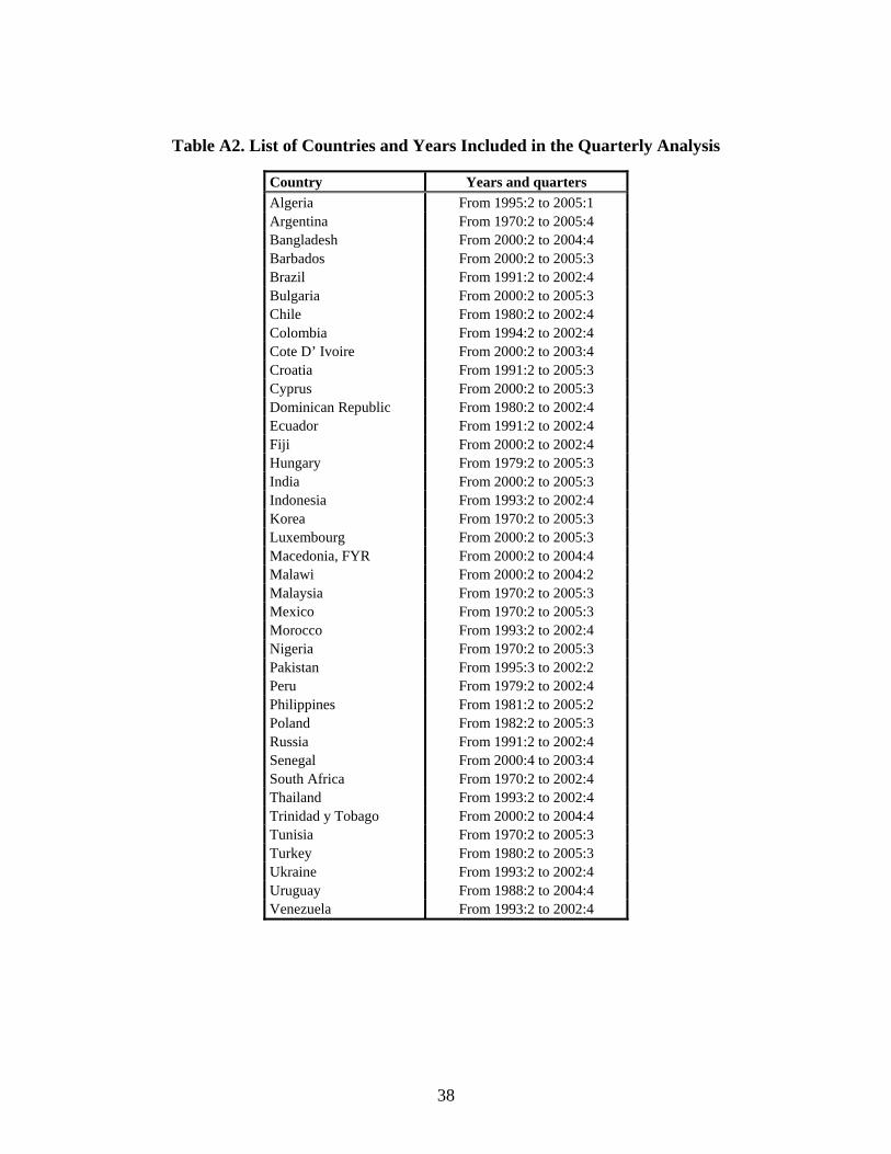
38

Table A2. List of Countries and Years Included in the Quarterly Analysis

Country Years and quarters Algeria From 1995:2 to 2005:1 Argentina From 1970:2 to 2005:4 Bangladesh From 2000:2 to 2004:4 Barbados From 2000:2 to 2005:3 Brazil From 1991:2 to 2002:4 Bulgaria From 2000:2 to 2005:3 Chile From 1980:2 to 2002:4 Colombia From 1994:2 to 2002:4 Cote D’ Ivoire From 2000:2 to 2003:4 Croatia From 1991:2 to 2005:3 Cyprus From 2000:2 to 2005:3 Dominican Republic From 1980:2 to 2002:4 Ecuador From 1991:2 to 2002:4 Fiji From 2000:2 to 2002:4 Hungary From 1979:2 to 2005:3 India From 2000:2 to 2005:3 Indonesia From 1993:2 to 2002:4 Korea From 1970:2 to 2005:3 Luxembourg From 2000:2 to 2005:3 Macedonia, FYR From 2000:2 to 2004:4 Malawi From 2000:2 to 2004:2 Malaysia From 1970:2 to 2005:3 Mexico From 1970:2 to 2005:3 Morocco From 1993:2 to 2002:4 Nigeria From 1970:2 to 2005:3 Pakistan From 1995:3 to 2002:2 Peru From 1979:2 to 2002:4 Philippines From 1981:2 to 2005:2 Poland From 1982:2 to 2005:3 Russia From 1991:2 to 2002:4 Senegal From 2000:4 to 2003:4 South Africa From 1970:2 to 2002:4 Thailand From 1993:2 to 2002:4 Trinidad y Tobago From 2000:2 to 2004:4 Tunisia From 1970:2 to 2005:3 Turkey From 1980:2 to 2005:3 Ukraine From 1993:2 to 2002:4 Uruguay From 1988:2 to 2004:4 Venezuela From 1993:2 to 2002:4

Economy & Finance

Elusive costs of sovereign defaults