Pressure Measurement
Theory and Application Guide
White Paper
Engineered solutions for all
applications

2 TI/266-EN | 2600T Series Pressure transmitters
The CompanyWe are an established world leader in the design and manufacture of measurement products for industrial process control, fl ow
measurement, gas and liquid analysis and environmental applications.
As a part of ABB, a world leader in process automation technology, we offer customers application expertise, service and support
worldwide.
We are committed to teamwork, high quality manufacturing, advanced technology and unrivalled service and support.
The quality, accuracy and performance of the Company’s products result from over 100 years experience, combined with
acontinuous program of innovative design and development to incorporate the latest technology.
2600T Series Pressure transmitters | TI/266-EN 3
Contents
Index
1. Introduction ........................................................... 5
2. Pressure measurement .......................................... 5 2.1 Atmospheric Pressure ...............................................5
2.2 Barometric Pressure ..................................................5
2.3 Hydrostatic Pressure ................................................5
2.4 Line Pressure ............................................................5
2.5 Static Pressure ..........................................................5
2.6 Working Pressure .....................................................5
2.7 Absolute Pressure .....................................................5
2.8 Gauge Pressure ........................................................5
2.9 Vacuum ....................................................................5
3. Pressure transmitter applications ........................ 6 3.1 Differential Pressure...................................................6
3.2 Flow .......................................................................6
3.3 Liquid level ...............................................................6
3.3.1 Open tank .......................................................6
3.3.2 Closed tank .....................................................6
3.3.3 Calculations ....................................................7
3.3.4 Bubble tube measurement ...............................7
3.4 Interface level measurement ......................................7
3.5 Density measurement ...............................................7
4. Pressure transmitter features ............................... 8 4.1 Main components .....................................................8
4.2 Measuring principle ...................................................9
4.2.1 Electromechanical strain gauge ........................9
4.2.2 Variable Capacitance ......................................9
4.2.3 Variable Reluctance .......................................10
4.2.4 Piezoresistive ................................................10
4.3 Signal Transmission .................................................10
4.3.1 Four-Wire Transmission ..................................10
4.3.2 Two-Wire Transmission ..................................10
4.3.3 “Smart” Transmission ....................................11
4.3.4 Fieldbus Transmission ...................................11
4.3.5 Loop Load Capacity ......................................11
4.4 Remote seals ..........................................................12
4.4.1 Remote seal response time ...........................12
4.4.2 Remote seal temperature effect .....................13
4.4.3 The all-welded construction technology ..........13
4.4.4 Remote seal applications ..............................13
5. Transmitter selection acc. to the application .......... 14 5.1 Pressure – differential, gauge or absolute .................14
5.1.1 Pipe or direct connected transmitters ............14
5.1.2 Direct-mounted diaphragm transmitters .........15
5.1.3 Remote seal transmitters .............................15
5.1.4 Remote seal transmitters for vacuum ..............16
5.2 Flow 16
5.2.1 Primary element .............................................16
5.2.2 Pressure transmitter ......................................16
5.2.3 Multivariable transmitter ...............................16
5.3 Level .....................................................................17
5.3.1 Open tank .....................................................17
5.3.2 Closed tank ...................................................17
5.4 Density ...................................................................18
5.5 Interface level .........................................................18
5.6 Volume (of product in a tank) ...................................19
6. Selection of transmitter’s features ...................... 20 6.1 Materials selection ..................................................20
6.1.1 Wetted parts material .....................................20
6.1.2 Housing ........................................................21
6.1.3 Fill fluid..........................................................21
6.1.4 Gasket ..........................................................21
6.2 Overpressure limits ..................................................21
6.3 Temperature limits ...................................................21
6.4 Accuracy ................................................................21
6.5 Power Surges .........................................................22
6.6 Safety .....................................................................22
6.6.1 Electrical Safety .............................................22
6.6.2 Safety Transmitters ........................................23
6.6.3 Pressure Safety .............................................24
6.6.4 Other safety considerations ............................24
4 TI/266-EN | 2600T Series Pressure transmitters
Contents
7. Transmitter terminology ...................................... 25 7.1 Accuracy ................................................................25
7.2 Reference Accuracy ................................................25
7.3 Damping ................................................................25
7.4 Dead band ..............................................................25
7.5 Drift .....................................................................25
7.6 Elevation and suppression ......................................26
7.7 Hysteresis ...............................................................27
7.8 Linearity ..................................................................27
7.8.1 Independent linearity .....................................27
7.8.2 Terminal-based linearity .................................28
7.8.3 Zero-based linearity ......................................28
7.9 Maximum Withstanded Pressure (MWP) ..................28
7.10 Output .................................................................28
7.11 Pressure ...............................................................28
7.11.1 Pressure definition from physic .....................28
7.11.2 Atmospheric pressure ..................................28
7.11.3 Overpressure ...............................................28
7.11.4 Proof pressure .............................................28
7.11.5 Absolute pressure ........................................28
7.11.6 Barometric pressure .....................................28
7.11.7 Differential pressure .....................................28
7.11.8 Gauge pressure ...........................................28
7.11.9 Hand Held Terminal ......................................28
7.11.10 Hydrostatic pressure ..................................28
7.11.11 Line pressure .............................................28
7.11.12 Static pressure ..........................................28
7.11.13 Vacuum .....................................................28
7.11.14 Working pressure .......................................29
7.12 Range ..................................................................29
7.12.1 Lower Range Value (LRV) .............................29
7.12.2 Upper Range Value (URV) .............................29
7.12.3 Lower Range Limit (LRL) ..............................29
7.12.4 Upper Range Limit (URL) ..............................29
7.12.5 Overrange ...................................................29
7.13 Reference operating conditions ..............................29
7.14 Repeatability .........................................................29
7.15 Reproducibility .....................................................29
7.16 Static pressure effect .............................................29
7.17 Span ...................................................................29
7.18 Span error ...........................................................29
7.19 Temperature effect ...............................................30
7.20 Turn Down ...........................................................30
7.21 Vibration effect ......................................................30
7.22 Zero error .............................................................30
2600T Series Pressure transmitters | TI/266-EN 5
1. Introduction / 2. Pressure measurement
1. IntroductionThis document has been prepared for individuals having moderate or little knowledge of electronic pressure transmitters products and their applications.
The first part of this document provides some definitions of the basic terminology used in the specification of a pressure transmitter. While in the second part it is provided a guide to the selection of pressure transmitters, including calculations examples required for the most common pressure transmitter applications.
PLEASE NOTE: the contents of this guide are for educational purposes only. Expert help should be obtained when specifying and installing a pressure measurement solution in any real-world application.
2. Pressure measurementA pressure transmitter like the ABB 2600T series can be used
to measure various forms of pressure. It can be used to
measure gauge pressure (barg, psig), absolute pressure (bara,
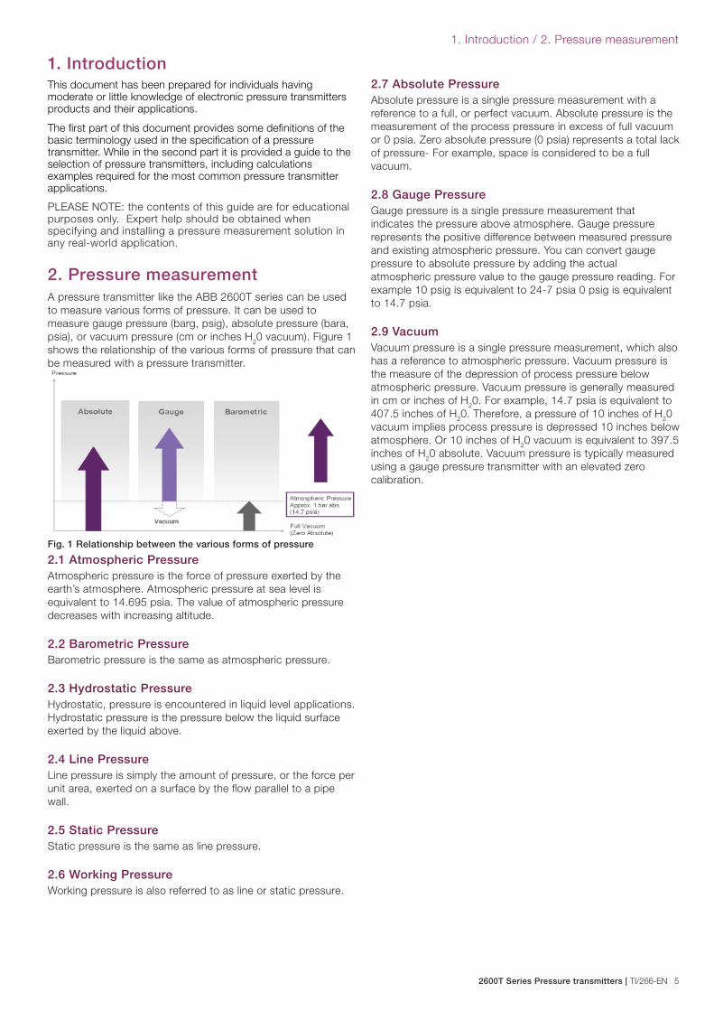
psia), or vacuum pressure (cm or inches H20 vacuum). Figure 1
shows the relationship of the various forms of pressure that can
be measured with a pressure transmitter.
2.1 Atmospheric PressureAtmospheric pressure is the force of pressure exerted by the
earth’s atmosphere. Atmospheric pressure at sea level is
equivalent to 14.695 psia. The value of atmospheric pressure
decreases with increasing altitude.
2.2 Barometric PressureBarometric pressure is the same as atmospheric pressure.
2.3 Hydrostatic Pressure Hydrostatic, pressure is encountered in liquid level applications.
Hydrostatic pressure is the pressure below the liquid surface
exerted by the liquid above.
2.4 Line PressureLine pressure is simply the amount of pressure, or the force per
unit area, exerted on a surface by the fl ow parallel to a pipe
wall.
2.5 Static PressureStatic pressure is the same as line pressure.
2.6 Working Pressure Working pressure is also referred to as line or static pressure.
Fig. 1 Relationship between the various forms of pressure
2.7 Absolute PressureAbsolute pressure is a single pressure measurement with a
reference to a full, or perfect vacuum. Absolute pressure is the
measurement of the process pressure in excess of full vacuum
or 0 psia. Zero absolute pressure (0 psia) represents a total lack
of pressure- For example, space is considered to be a full
vacuum.
2.8 Gauge PressureGauge pressure is a single pressure measurement that
indicates the pressure above atmosphere. Gauge pressure
represents the positive difference between measured pressure
and existing atmospheric pressure. You can convert gauge
pressure to absolute pressure by adding the actual
atmospheric pressure value to the gauge pressure reading. For
example 10 psig is equivalent to 24-7 psia 0 psig is equivalent
to 14.7 psia.
2.9 VacuumVacuum pressure is a single pressure measurement, which also
has a reference to atmospheric pressure. Vacuum pressure is
the measure of the depression of process pressure below
atmospheric pressure. Vacuum pressure is generally measured
in cm or inches of H20. For example, 14.7 psia is equivalent to
407.5 inches of H20. Therefore, a pressure of 10 inches of H
20
vacuum implies process pressure is depressed 10 inches below
atmosphere. Or 10 inches of H20 vacuum is equivalent to 397.5
inches of H20 absolute. Vacuum pressure is typically measured
using a gauge pressure transmitter with an elevated zero
calibration.
6 TI/266-EN | 2600T Series Pressure transmitters
3. Pressure transmitter applications
3. Pressure transmitter applications Pressure is considered a basic measurement because it is
utilized in several process applications: pressure and differential
pressure, fl ow, level, density, etc. This section will briefl y
describe the following measurement applications that
transmitters such as the ABB 2600T can be used for.
3.1 Differential PressureDifferential pressure is the difference in magnitude between
some pressure value and a reference pressure. In a sense,
absolute pressure can also be considered a differential
pressure, with full vacuum or zero absolute as the reference
pressure. Gauge pressure too can be considered a differential
pressure, since in gauge pressure the atmospheric pressure is
the reference pressure.
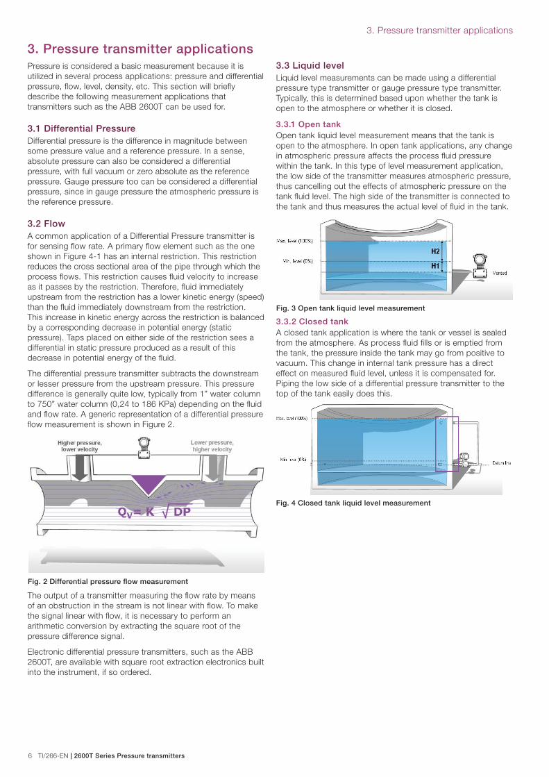
3.2 FlowA common application of a Differential Pressure transmitter is
for sensing fl ow rate. A primary fl ow element such as the one
shown in Figure 4-1 has an internal restriction. This restriction
reduces the cross sectional area of the pipe through which the
process fl ows. This restriction causes fl uid velocity to increase
as it passes by the restriction. Therefore, fl uid immediately
upstream from the restriction has a lower kinetic energy (speed)
than the fl uid immediately downstream from the restriction.
This increase in kinetic energy across the restriction is balanced
by a corresponding decrease in potential energy (static
pressure). Taps placed on either side of the restriction sees a
differential in static pressure produced as a result of this
decrease in potential energy of the fl uid.
The differential pressure transmitter subtracts the downstream
or lesser pressure from the upstream pressure. This pressure
difference is generally quite low, typically from 1” water column
to 750” water column (0,24 to 186 KPa) depending on the fl uid
and fl ow rate. A generic representation of a differential pressure
fl ow measurement is shown in Figure 2.
Fig. 2 Differential pressure fl ow measurement
The output of a transmitter measuring the fl ow rate by means
of an obstruction in the stream is not linear with fl ow. To make
the signal linear with fl ow, it is necessary to perform an
arithmetic conversion by extracting the square root of the
pressure difference signal.
Electronic differential pressure transmitters, such as the ABB
2600T, are available with square root extraction electronics built
into the instrument, if so ordered.
3.3 Liquid levelLiquid level measurements can be made using a differential
pressure type transmitter or gauge pressure type transmitter.
Typically, this is determined based upon whether the tank is
open to the atmosphere or whether it is closed.
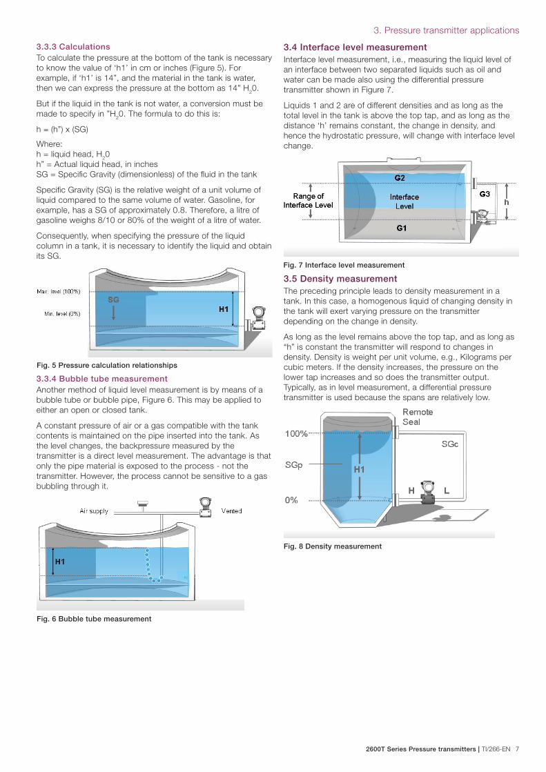
3.3.1 Open tankOpen tank liquid level measurement means that the tank is
open to the atmosphere. In open tank applications, any change
in atmospheric pressure affects the process fl uid pressure
within the tank. In this type of level measurement application,
the low side of the transmitter measures atmospheric pressure,
thus cancelling out the effects of atmospheric pressure on the
tank fl uid level. The high side of the transmitter is connected to
the tank and thus measures the actual level of fl uid in the tank.
Fig. 3 Open tank liquid level measurement
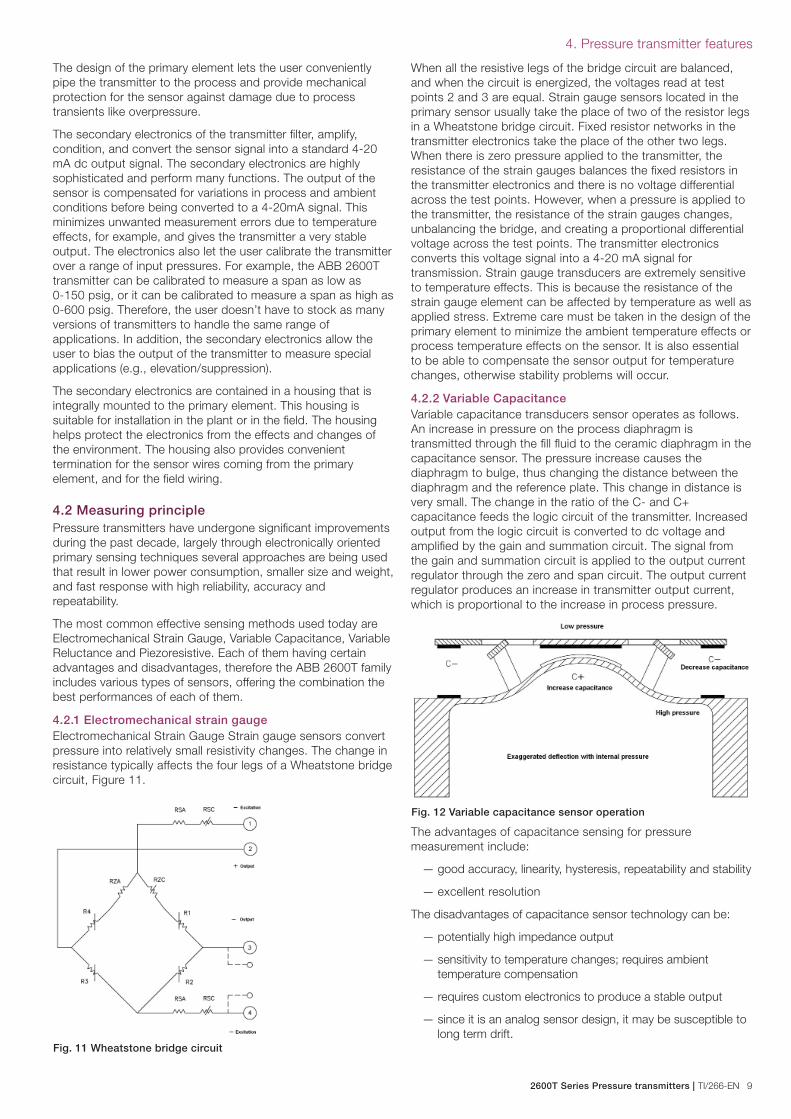
3.3.2 Closed tankA closed tank application is where the tank or vessel is sealed
from the atmosphere. As process fl uid fi lls or is emptied from
the tank, the pressure inside the tank may go from positive to
vacuum. This change in internal tank pressure has a direct
effect on measured fl uid level, unless it is compensated for.
Piping the low side of a differential pressure transmitter to the
top of the tank easily does this.
Fig. 4 Closed tank liquid level measurement
2600T Series Pressure transmitters | TI/266-EN 7
3. Pressure transmitter applications
3.3.3 CalculationsTo calculate the pressure at the bottom of the tank is necessary
to know the value of ‘h1’ in cm or inches (Figure 5). For
example, if ‘h1’ is 14”, and the material in the tank is water,
then we can express the pressure at the bottom as 14” H20.
But if the liquid in the tank is not water, a conversion must be
made to specify in ”H20. The formula to do this is:
h = (h”) x (SG)
Where:
h = liquid head, H20
h” = Actual liquid head, in inches
SG = Specifi c Gravity (dimensionless) of the fl uid in the tank
Specifi c Gravity (SG) is the relative weight of a unit volume of
liquid compared to the same volume of water. Gasoline, for
example, has a SG of approximately 0.8. Therefore, a litre of
gasoline weighs 8/10 or 80% of the weight of a litre of water.
Consequently, when specifying the pressure of the liquid
column in a tank, it is necessary to identify the liquid and obtain
its SG.
Fig. 5 Pressure calculation relationships
3.3.4 Bubble tube measurementAnother method of liquid level measurement is by means of a
bubble tube or bubble pipe, Figure 6. This may be applied to
either an open or closed tank.
A constant pressure of air or a gas compatible with the tank
contents is maintained on the pipe inserted into the tank. As
the level changes, the backpressure measured by the
transmitter is a direct level measurement. The advantage is that
only the pipe material is exposed to the process - not the
transmitter. However, the process cannot be sensitive to a gas
bubbling through it.
Fig. 6 Bubble tube measurement
3.4 Interface level measurementInterface level measurement, i.e., measuring the liquid level of
an interface between two separated liquids such as oil and
water can be made also using the differential pressure
transmitter shown in Figure 7.
Liquids 1 and 2 are of different densities and as long as the
total level in the tank is above the top tap, and as long as the
distance ‘h’ remains constant, the change in density, and
hence the hydrostatic pressure, will change with interface level
change.
Fig. 7 Interface level measurement
3.5 Density measurement The preceding principle leads to density measurement in a
tank. In this case, a homogenous liquid of changing density in
the tank will exert varying pressure on the transmitter
depending on the change in density.
As long as the level remains above the top tap, and as long as
“h” is constant the transmitter will respond to changes in
density. Density is weight per unit volume, e.g., Kilograms per
cubic meters. If the density increases, the pressure on the
lower tap increases and so does the transmitter output.
Typically, as in level measurement, a differential pressure
transmitter is used because the spans are relatively low.
Fig. 8 Density measurement

8 TI/266-EN | 2600T Series Pressure transmitters
4. Pressure transmitter features
4. Pressure transmitter features As already mentioned, pressure is considered a basic measurement because it is utilized in several process applications: pressure
and differential pressure, fl ow, level, density, volume, etc.
4.1 Main componentsPressure is measured by means of transmitters that generally consist of two main parts: a sensing element, which is in direct or
indirect contact with the process, and a secondary electronic package which translates and conditions the output of the sensing
element into a standard transmission signal.
1
2
3
4
5
6
8
7
9
10
11
12
12
13
13
14
14
15
15
16
17
18
19 20
1 Rear cover | 2 Terminal block | 3 Push buttons | 4 Housing | 5 Communication board | 6 Front blind cover | 7 Display connector | 8 LCD display with keypad | 9 LCD display with keypad and TTG technology | 10 Standard LCD display | 11 Front windowed cover | 12 Flange adapter | 13 Low rating fl anges | 14 Standard process fl anges | 15 Transducer gasket | 16 Transducer | 17 Plug | 18 Vent/drain valve | 19 Bracket kit for pipe or wall mounting | 20 Flat type bracket kit for box Fig. 9 Differential pressure transmitter components
At the heart of the transducer there is a sensor that creates a
low level electronic signal in response to force applied against
the sensing element. The sensor in the ABB 2600T Transmitter
has different working principle as detailed in the following
paragraphs. The sensor does not come into contact with the
process, but is protected from it by the use of isolating
diaphragm(s) and a fi ll fl uid.
Pascal’s Law states that whenever an external pressure is
applied to any confi ned fl uid at rest, the pressure is increased at
every point in the fl uid by the amount of that external pressure.
This is the basic principle employed in primary element design.
The primary element is connected to the process piping in such
a way that the process pressure is exerted against the isolation
diaphragm(s). According to Pascal’s Law, the fi ll fl uid inside the
primary element will reach the same pressure as that applied
against the isolation diaphragm(s). The fi ll fl uid hydraulically
conveys this pressure to the sensor, which in turn produces an
appropriate output signal.
The design of the primary element lets the user conveniently
pipe the transmitter to the process and provide mechanical
protection for the sensor against damage due to process
transients like overpressure. Fig. 10 Transducer components
1 Primary electronic | 2 Transducer body | 3 Inductive sensor | 4 Idraulic circuit components | 5 Gasket | 6 Isolating diaphragm
1
2
2
3
4
56
2600T Series Pressure transmitters | TI/266-EN 9
4. Pressure transmitter features
The design of the primary element lets the user conveniently
pipe the transmitter to the process and provide mechanical
protection for the sensor against damage due to process
transients like overpressure.
The secondary electronics of the transmitter fi lter, amplify,
condition, and convert the sensor signal into a standard 4-20
mA dc output signal. The secondary electronics are highly
sophisticated and perform many functions. The output of the
sensor is compensated for variations in process and ambient
conditions before being converted to a 4-20mA signal. This
minimizes unwanted measurement errors due to temperature
effects, for example, and gives the transmitter a very stable
output. The electronics also let the user calibrate the transmitter
over a range of input pressures. For example, the ABB 2600T
transmitter can be calibrated to measure a span as low as
0-150 psig, or it can be calibrated to measure a span as high as
0-600 psig. Therefore, the user doesn’t have to stock as many
versions of transmitters to handle the same range of
applications. In addition, the secondary electronics allow the
user to bias the output of the transmitter to measure special
applications (e.g., elevation/suppression).
The secondary electronics are contained in a housing that is
integrally mounted to the primary element. This housing is
suitable for installation in the plant or in the fi eld. The housing
helps protect the electronics from the effects and changes of
the environment. The housing also provides convenient
termination for the sensor wires coming from the primary
element, and for the fi eld wiring.
4.2 Measuring principlePressure transmitters have undergone signifi cant improvements
during the past decade, largely through electronically oriented
primary sensing techniques several approaches are being used
that result in lower power consumption, smaller size and weight,
and fast response with high reliability, accuracy and
repeatability.
The most common effective sensing methods used today are
Electromechanical Strain Gauge, Variable Capacitance, Variable
Reluctance and Piezoresistive. Each of them having certain
advantages and disadvantages, therefore the ABB 2600T family
includes various types of sensors, offering the combination the
best performances of each of them.
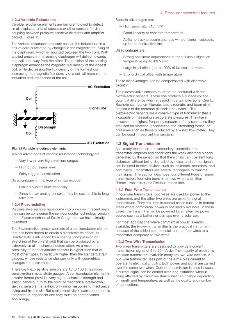
4.2.1 Electromechanical strain gaugeElectromechanical Strain Gauge Strain gauge sensors convert
pressure into relatively small resistivity changes. The change in
resistance typically affects the four legs of a Wheatstone bridge
circuit, Figure 11.
When all the resistive legs of the bridge circuit are balanced,
and when the circuit is energized, the voltages read at test
points 2 and 3 are equal. Strain gauge sensors located in the
primary sensor usually take the place of two of the resistor legs
in a Wheatstone bridge circuit. Fixed resistor networks in the
transmitter electronics take the place of the other two legs.
When there is zero pressure applied to the transmitter, the
resistance of the strain gauges balances the fi xed resistors in
the transmitter electronics and there is no voltage differential
across the test points. However, when a pressure is applied to
the transmitter, the resistance of the strain gauges changes,
unbalancing the bridge, and creating a proportional differential
voltage across the test points. The transmitter electronics
converts this voltage signal into a 4-20 mA signal for
transmission. Strain gauge transducers are extremely sensitive
to temperature effects. This is because the resistance of the
strain gauge element can be affected by temperature as well as
applied stress. Extreme care must be taken in the design of the
primary element to minimize the ambient temperature effects or
process temperature effects on the sensor. It is also essential
to be able to compensate the sensor output for temperature
changes, otherwise stability problems will occur.
4.2.2 Variable Capacitance Variable capacitance transducers sensor operates as follows.
An increase in pressure on the process diaphragm is
transmitted through the fi ll fl uid to the ceramic diaphragm in the
capacitance sensor. The pressure increase causes the
diaphragm to bulge, thus changing the distance between the
diaphragm and the reference plate. This change in distance is
very small. The change in the ratio of the C- and C+
capacitance feeds the logic circuit of the transmitter. Increased
output from the logic circuit is converted to dc voltage and
amplifi ed by the gain and summation circuit. The signal from
the gain and summation circuit is applied to the output current
regulator through the zero and span circuit. The output current
regulator produces an increase in transmitter output current,
which is proportional to the increase in process pressure.
Fig. 11 Wheatstone bridge circuit
Fig. 12 Variable capacitance sensor operation
The advantages of capacitance sensing for pressure
measurement include:
— good accuracy, linearity, hysteresis, repeatability and stability
— excellent resolution
The disadvantages of capacitance sensor technology can be:
— potentially high impedance output
— sensitivity to temperature changes; requires ambient
temperature compensation
— requires custom electronics to produce a stable output
— since it is an analog sensor design, it may be susceptible to
long term drift.
10 TI/266-EN | 2600T Series Pressure transmitters
4. Pressure transmitter features
4.2.3 Variable ReluctanceVariable reluctance elements are being employed to detect
small displacements of capsules or other sensors for direct
coupling between pressure sensitive elements and amplifi er
circuits, Figure 13.
The variable reluctance pressure sensor, the inductance in a
pair of coils is affected by changes in the magnetic coupling of
the diaphragm, which is mounted between the two coils. With
applied pressure, the sensing diaphragm will defl ect towards
one coil and away from the other. The position of the sensing
diaphragm enhances the magnetic fl ux density of the closest
coil, while decreasing the fl ux density of the furthest coil.
Increasing the magnetic fl ux density of a coil will increase the
induction and impedance of the coil.
Fig. 13 Variable reluctance elements
Typical advantages of variable reluctance technology are:
— Very low or very high pressure ranges.
— High output signal level.
— Fairly rugged construction
Disadvantages of this type of sensor include:
— Limited overpressure capability.
— Since it is an analog sensor, it may be susceptible to long
term drift.
4.2.4 PiezoresistivePiezoresistive sensors have come into wide use in recent years,
they can be considered the semiconductor technology version
of the Electromechanical Strain Gauge that we have already
described.
The Piezoresistive sensor consists of a semiconductor element
that has been doped to obtain a piezoresistive effect. Its
Conductivity is infl uenced by a change (compression or
stretching of the crystal grid) that can be produced by an
extremely small mechanical deformation. As a result, the
sensitivity of monocrystalline sensors is higher than that of
most other types. In particular higher than the standard strain
gauges, whose resistance changes only with geometrical
changes in the structure.
Therefore Piezoresistive sensors are 10 to 100 times more
sensitive than metal strain gauges. A semiconductor element in
a wafer format provides very high mechanical strength and
elastic behaviour up to the point of mechanical breakdown,
yielding sensors that exhibit only minor response to mechanical
aging and hysteresis. But strain sensitivity in semiconductors is
temperature dependent and they must be compensated
accordingly.
Specifi c advantages are:
— High sensitivity, >10mV/V
— Good linearity at constant temperature
— Ability to track pressure changes without signal hysteresis,
up to the destructive limit
Disadvantages are:
— Strong non linear dependence of the full-scale signal on
temperature (up to 1%/kelvin)
— Large initial offset (up to 100% of full scale or more)
— Strong drift of offset with temperature
These disadvantages can be compensated with electronic
circuitry.
The piezoresistive sensors must not be confused with the
piezoelectric sensors. These one produce a surface voltage
potential difference when stressed in certain directions. Quartz,
Rochelle salt, barium titanate, lead-zirconate, and tourmaline
are some of the common piezoelectric crystals. The
piezoelectric sensors are a dynamic type of transducer that is
incapable of measuring steady-state pressures. They have,
however, the highest frequency response of any sensor, so they
are used for vibration, acceleration and alternating forces, or
pressures such as those produced by a vortex fl ow meter. They
can be used in resonant transmitters.
4.3 Signal TransmissionAs already mentioned, the secondary electronics of a
transmitter amplifi es and conditions the weak electrical signals
generated by the sensor, so that the signals can’t be sent long
distances without being degraded by noise, and so the signals
can be used to drive devices such as indicators, recorders, and
controllers. Transmitters use several techniques to transmit
their signal. This section describes four different types of signal
transmission: four-wire transmitter, two wire transmitter,
“Smart” transmitter and Fieldbus transmitter.
4.3.1 Four-Wire TransmissionIn four-wire transmitters, two wires are used for power to the
instrument, and the other two wires are used for signal
transmission. They are used in special cases such as in remote
areas where commercial power is not readily available. In these
cases, the transmitter will be powered by an alternate power
source such as a battery or perhaps even a solar cell.
For most applications where commercial power is readily
available, the two-wire transmitter is the practical instrument,
because of the added cost to install and run four wires to a
transmitter compared to two wires.
4.3.2 Two-Wire TransmissionTwo wires transmitters are designed to provide a current
transmission signal of 4 to 20 mA dc. The majority of electronic
pressure transmitters available today are two-wire devices. A
two-wire transmitter uses part of the 4 mA bias current to
operate its electrical circuitry. Both power and signal are carried
over the same two wires. Current transmission is used because
a current signal can be carried over long distances without
being affected by circuit resistance that can change depending
on length and temperature, as well as the quality and number
of connections.

2600T Series Pressure transmitters | TI/266-EN 11
4. Pressure transmitter features
4.3.3 “Smart” Transmission Intelligent or “Smart” transmitters transmit both digital and
analog signals over the same two wires. A digital signal is
superimposed over the traditional 4 to 20 mA.
Digital signal transmission is faster and more accurate than
analog. More information can be carried between the
instrument and the control room using the same two wires with
two-way digital transmission, including confi guration and
diagnostic information.
Two-way communications means that a value cannot only be
read from the end device but it is possible to write to the
device. For example, the calibration constants associated with
a particular sensor can now be stored directly in the device
itself and changed as needed. This often makes it possible to
remotely diagnose a fi eld device problem, thus saving a costly
trip to the fi eld. The most widespread digital communication is
HART® based on Bell 202 FSK standard, there are millions of
instruments in the world using this standard, it is simple and
well understood.
4.3.4 Fieldbus Transmission Fieldbus is a digital, two-way, multi-drop communication link
among intelligent control devices that can be used only instead
of the 4-20 mA standard.
Multi drop communication means that over the same two wires
can take place a digital communication among several fi eld
devices (like valves, pressure transducers, etc.) and computers,
programmable logic controllers (PLCs) or remote terminal units
(RTUs). The multi-drop capability of a fi eldbus will perhaps
result in the most immediate cost saving benefi t for users, since
one single wire pair is shared among several devices. While
with analog or smart devices, a separate cable needs to be run
between each end device and the control system.
Profi bus and Fieldbus Foundation (FF) are probably the most
widespread fi eldbuses. The main advantage of FF is that it
allows the relocation of control functions (like the PID) from the
central control room out to the fi eldbus devices. In this way a
loop can e realized through the direct communication between
a sensor and a control valve. This results in better, more reliable
control as well as a less complex centralized control system.
The current limitation is on communication speed and the
limited maximum number of instrument linked to the same
communication “segment”.
The main advantage of Profi bus is that it is well suited also for
digital signal transmission. Therefore it is often selected in
processes with a high number of digital signals (like batch
processes or manufacturing industries). It can reach higher
communication speed in the traditional master slave
confi guration, where a controller acquired data from the
transmitter and sets the values of the valve. In case of failure of
the main master a reserve master can take over the
communication.
4.3.5 Loop Load CapacityTwo-wire transmitters must have a certain minimum voltage at
the terminals in order to function. Typically this value is 12Vdc.
Figure 14 shows a two-wire circuit.
With a 24V dc power supply, and the transmitter requiring
12Vdc at its terminals, this leaves only the difference, or 12Vdc,
for voltage drops around the loop.
In terms of resistance, by applying Ohm’s Law of R = E/I, and
noting that the maximum analog signal is 20 mA or .020 Amps,
we can compute the maximum resistance allowed in the loop:
R = E/I = 12 Vdc / 0.02 A = 600 Ohms
Note that, according to Namur standards, the maximum
current output can be conventionally set to 22 mA. The
transmitter in case of main transmitter failure conditions
detected by self-diagnostic sets this output. If this feature is to
be used, the maximum current value in the above calculation
has to be modifi ed accordingly with a 0.22 A instead of 0.20 A.
Fig. 14 Load loop capacity
To derive the total loop resistance we add:
250 Ohms Typical Load Resistor
45 Ohms Line Resistance (varies with length and size, but
this value is typically used for design purposes)
70 Ohms Surge Protector_________
365 Ohms Total Loop Resistance (Loop Load)
This loop will operate satisfactorily having a 235 Ohm surplus
load capability. (600 - 365 = 235 Ohms).
The ABB 2600T transmitters can operate with up to a 55Vdc
power supply. This increases the load carrying capability of the
loop to
R = (55-12)/0.020 = 2150 Ohms
In case the DC power supply is increased, a minimum load
resistance has to be present in order to avoid damages to the
electronic circuitry. The addition of other resistances, such as
barriers in an intrinsically safe loop, must be carefully
considered in determining the total loop resistance. You may
fi nd specifi cation sheets use the term impedance for dc
resistance. This is a convention in the instrument business.

12 TI/266-EN | 2600T Series Pressure transmitters
4. Pressure transmitter features
4.4 Remote sealsRemote seals have been developed in order to widen the applicability of pressure transmitter beyond their limitations in terms of
maximum temperature, dirty process fl uids, etc..
This section describes the features of remote seal transmitters and the impact on their response time and the temperature effect
on its precision. For some guidelines on the selection of the appropriate remote seal, see the following chapter on applications.
A remote seals consists of a remote element made up of a fl ange connection, a stem, and a seal diaphragm with a membrane
connected through a capillary to the fl anged chamber of the transmitter.
The remote seal can be integral with the transmitter or remote with a capillary length up to some meters. In this case the capillary
is protected with suitable armour. Once connected the individual components, the system is evacuated from the air and fi lled with
an incompressible fl uid.
In this way when process pressure is applied to the seal diaphragm, this one defl ects and exerts a force against the fi ll fl uid. Since
the liquid is incompressible, this force is transmitted hydraulically to the sensing diaphragm in the transmitter body, causing it in
turn to defl ect. The defl ection of the sensing diaphragm of the transmitter is the basis for the pressure measurement. For a proper
dimensioning of a remote seal system some features has to be considered. The fi rst one is the displacement capacity (i.e. the
volume displacement in the transmitter resulting from a full scale defl ection of the seal). It must exceed the displacement capacity
of the transmitter; otherwise the seal element cannot drive the transmitter to full-scale measurement.The second one is the
volume of the cavity between the fl ange and the primary isolation diaphragm of the transmitter. The total volume of fi ll fl uid has to
be minimized in order to minimize the ambient / process temperature effect (see the paragraph on temperature effect in the
following). Special fl anges are available for the transmitters that minimize the cavity volume when connected to a remote seal.
With the ABB 2600T product family, that includes both transmitters and remote seals, the above mentioned features are already
taken into account and the assembly is properly optimised.
4.4.1 Remote seal response time The response time is qualifi ed by means of the time constant, i.e. the amount of time required for an instrument output to reach
the 63% of the amount it will ultimately change in response to a step change in input. Normally an instrument will reach 99.9 % of
full response within a length of time equal to four times the time constant. The response time of a transmitter can be signifi cantly
increased when connected to a remote seal. This response time is affected by:
— The total length of capillary connecting the seal element to the transmitter body. The response time is directly proportional to
the length of capillary. Therefore the length of capillary has to be minimized provided that the application requirements are
satisfi ed.
— The inside diameter of the capillary. The response time of the instrument is inversely proportional to the fourth power of the
capillary diameter. A smaller capillary section “delays” the response.
— The fl uid viscosity. It is intuitive that a high viscosity of the fl uid increases the time it will take that fl uid to transmit an applied
force through the system. Also the temperature effect on viscosity (generally the viscosity increases as temperature
decreases) has to be considered, in particular it is important the temperature along the length of the capillary. The lower this
average temperature, the slower the response time of the system.
Fig. 15 Seal system structure
2600T Series Pressure transmitters | TI/266-EN 13
4. Pressure transmitter features
4.4.2 Remote seal temperature effect A change in temperature from the temperature under which the
system was fi lled (we can call it the reference temperature) will
cause the fi ll fl uid to expand or contract. The resulting effect
depends on the physical properties of the actual fi ll fl uid being
used. The change in volume causes the internal pressure of the
system to change. This will in turn cause a defl ection in the
diaphragm, which leads to zero shifts and unwanted
measurement errors. After installation this effect can be “zeroed
out”. However each time there is a temperature variation in the
process or ambient temperature, which affects the temperature
of one or more components of the remote seal, a measurement
error will be induced. A simplifi cation factor applies in case of
differential pressure measurement with two remote seals that
have the same dimensions, including the capillary length. If the
temperature of both branches of the transmitter is the same,
the effect on the differential pressure transmitter will
compensate each other, minimizing the error.
Another feature of the remote seals that attenuates the
temperature effect is low seal diaphragm stiffness. This is
measured as a spring rate, i.e. a pressure variation applied
divided by the resulting volumetric displacement. Less stiff
diaphragms will have lower values of spring rate and will
produce a small increase of the pressure applied to the
transmitter as a result of a temperature increase.
Increasing the diameter of the diaphragm decreases its spring
rate. Low spring rate are also recommended for measuring very
low pressure spans, as they can withstand only small
volumetric changes in fi ll fl uid. The length of capillaries is
dictated by the installation, they could be better accomplished
in terms of response time by means of larger internal
diameters. But this, together with the length of capillary
increases the total volume of the fi lling fl uid, with a negative
temperature. Hence a trade-off between response time and
optimal temperature performance has to be accepted.
4.4.3 The all-welded construction technologyAnother critical source of error for the remote seal is the
possibility that any gas enter the capillary system. Because of
gas compressibility even a small quantity of gas prevents the
principle upon which the seal operate (i.e. absolute constant fi ll
fl uid volume at any pressure). Therefore special care must be
paid during the fi lling operations in order to carefully avoid any
gas penetration, i.e. fi ll fl uid is de-aerated, the dry remote seal
system is emptied at full vacuum prior to fi lling, then the system
is sealed and a leak test is carried out.
Nevertheless during the operation of the transmitter, a slow gas
penetration is possible through gasket connections or threaded
joints. This is even more critical because the system fails
“slowly” and larger errors occur prior to failure.
ABB was the fi rst to introduce an innovative technology that
consists in welding all the capillary connections including a
fi lling capillary welded shut (see the above fi gure). This
technology has proven to really guarantee that no air enters
system even after years of continuous service. These features
are absolutely mandatory for high vacuum service application
where even some microscopic amount of gas tends to expand
their volume tremendously as a pressure close to absolute zero
is reached.
4.4.4 Remote seal applications In pressure transmitter directly connected to process piping by
the use of impulse lines, the process fl uid leaves the piping, fi lls
the impulse lines and enters the body of the transmitter.
Remote seals are recommended for all applications where it is
necessary to prevent the fl uid to leave the piping, or to enter
the transmitter because of:
— The process fl uid is highly corrosive
— The process fl uid is dirty, solid laden, or viscous and can
foul the impulse line
— The process fl uid can solidify in impulse line or the
transmitter body, because of temperature decrease
— The process fl uid is too hazardous to enter the area where
the transmitter is located
— The transmitter body must be located away from the
process for easier maintenance
— The process temperature exceeds the recommended
maximum limits for the transmitter
The latter can also be accomplished using impulse lines of
suffi cient length. Remote seals are employed when required
impulse line length becomes impractical for the installation.
14 TI/266-EN | 2600T Series Pressure transmitters
5. Transmitter selection according to the application
5. Transmitter selection according to the applicationThe scope of this section is to help how to identify the
instrument type (differential, absolute, fl ange mounted, etc.) that
is suitable for a specifi c application. The features of the
instrument that have to be identifi ed include also Remote Seals
requirement, required measuring range, wetted parts material
(suggested or materials not recommended) special requirements
of fi ll fl uid and of overpressure limits.
The initial questions that are to be asked are:
— the required measure, i.e. Level, Flow , Pressure (gauge,
absolute), Differential Pressure, Liquid Interface Level,
Density, Volume (of product in a tank)
— the process conditions: process and ambient
Temperature, Pressure (in particular Vacuum conditions),
Flow and line size as appropriate
— the process fl uid and some of its properties like status:
gas, liquid, condensable vapour, freezing or jellying at
process or ambient temperature and its condition: clean,
dirty, with solid suspensions
5.1 Pressure – differential, gauge or absoluteGiven the process operating pressure range, it is possible to
determine if a gauge, absolute or (high) vacuum type of
instrument is necessary. First of all it is necessary to decide the
type of measure: Differential, Absolute or Gauge. At this purpose
it is necessary to look at the required measuring range.
Differential ranges are specifi ed in Kilo Pascal (i.e. 0 to 300 KPa)
or pounds per square inch (i.e. 0 to 45 psi) or inches of water
column (i.e. 0 to 100 inWC) or millimeters of water column (i.e. 0
to 2540 mmWC).
Gauge pressure ranges are usually expressed in pounds per
square inch gauge (i.e. pressure is referred to atmospheric
pressure, 0–100 psig) or in Bars (i.e. 0-69 Barsg). The range may
have a suppressed zero (i.e., 100 to 200 psig or 69-138 Barsg),
or it may be a compound range (i.e., 20 inHg vacuum to 45 psig
or 68 KPa abs to 310 KPag).
Absolute ranges are usually expressed in inches of mercury
absolute or psia (i.e., 0–30 HgA or 0–100 psia). The most
common range with a suppressed zero is the barometric range
(i.e., 28 to 32 inHgA or 9686 to 11070 mmWCa).
Another way to fi nd out the type of measure is according to the
number of process connections: two connections to the process
are associated with a differential type of measure. In case of a
single connection to the process and a pressure range close to
Absolute Zero or that has to be independent from Atmospheric
Pressure variations, usually it is specifi ed the Absolute type of
measure, otherwise the Gauge type of measure is selected.
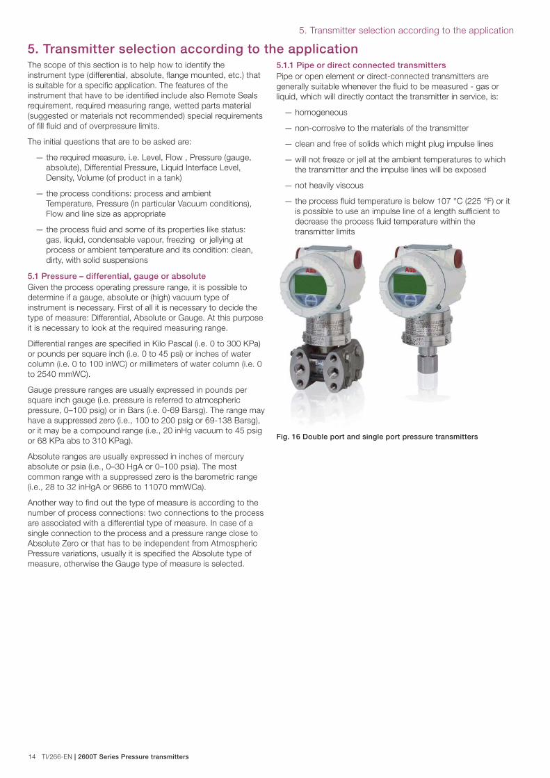
5.1.1 Pipe or direct connected transmitters Pipe or open element or direct-connected transmitters are
generally suitable whenever the fl uid to be measured - gas or
liquid, which will directly contact the transmitter in service, is:
— homogeneous
— non-corrosive to the materials of the transmitter
— clean and free of solids which might plug impulse lines
— will not freeze or jell at the ambient temperatures to which
the transmitter and the impulse lines will be exposed
— not heavily viscous
— the process fl uid temperature is below 107 °C (225 °F) or it
is possible to use an impulse line of a length suffi cient to
decrease the process fl uid temperature within the
transmitter limits
Fig. 16 Double port and single port pressure transmitters
2600T Series Pressure transmitters | TI/266-EN 15
5. Transmitter selection according to the application
5.1.2 Direct-mounted diaphragm transmitters A direct mount transmitter is practical in all cases where it is
possible to connect the transmitter directly to the process,
without the need of yokes for the transmitter and the connection
of impulse line. This is recommended when the process fl uid is
viscous or dirty; it contains solids that will precipitate or plug
impulse lines. In case the fl uid may freeze or jell at the ambient
temperature that will be encountered, an extended fl ush
diaphragm is more suitable.
Flange mounted transmitters are suggested also in case the
process fl uid is corrosive to the internal parts of the transmitter,
while it is available a seal material to which the fl uid is not
corrosive, i.e. the Tefl on anticorrosion and antistick coating. They
are also a solution when the process fl uid temperature is above
107 °C and below 210 °C (225 ° / 410 °F) and the use of
impulse line of a length suffi cient (to decrease the process fl uid
temperature within the transmitter limits) is not practical.
A direct mount diaphragm is required in case of food or
pharmaceutical application, since they require special seals in
order to assure the maximum possibility to clean the process
connection. Furthermore in this case also the fi lling fl uid must be
non-toxic, like Glycerine/Water, Vegetal or Mineral oils.
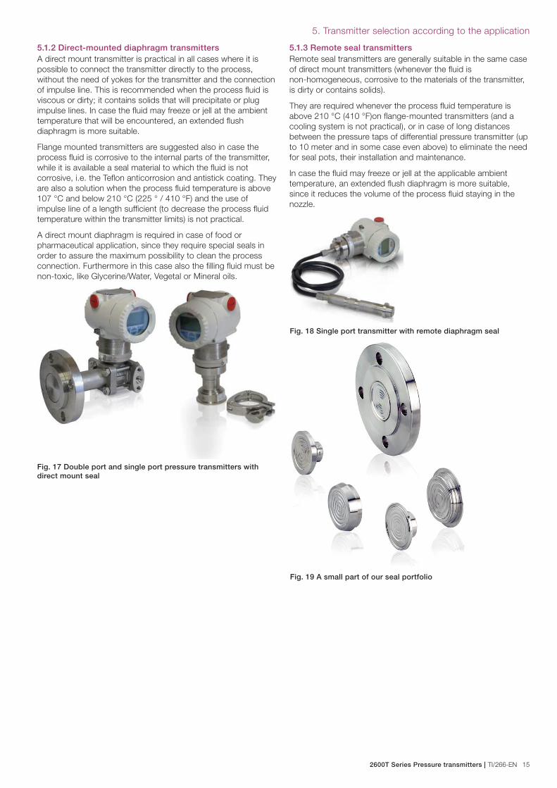
Fig. 17 Double port and single port pressure transmitters with direct mount seal
5.1.3 Remote seal transmitters Remote seal transmitters are generally suitable in the same case
of direct mount transmitters (whenever the fl uid is
non-homogeneous, corrosive to the materials of the transmitter,
is dirty or contains solids).
They are required whenever the process fl uid temperature is
above 210 °C (410 °F)on fl ange-mounted transmitters (and a
cooling system is not practical), or in case of long distances
between the pressure taps of differential pressure transmitter (up
to 10 meter and in some case even above) to eliminate the need
for seal pots, their installation and maintenance.
In case the fl uid may freeze or jell at the applicable ambient
temperature, an extended fl ush diaphragm is more suitable,
since it reduces the volume of the process fl uid staying in the
nozzle.
Fig. 18 Single port transmitter with remote diaphragm seal
Fig. 19 A small part of our seal portfolio
16 TI/266-EN | 2600T Series Pressure transmitters
5. Transmitter selection according to the application
5.1.4 Remote seal transmitters for vacuumThe relative position of the transmitter respect to the measuring
point must be taken into consideration: it is recommended to
install the transmitter below (or at) the High Side Datum.
For Differential Pressure transmitter application across a fan, no
Seal Transmitters are allowed, because the differential pressure
ranges are too little and usually no dirty or solid suspensions
are present.
Summarizing, in case the fl uid is clean it is possible to use an
instrument with a direct connection to the process, otherwise in
case of dirty or fl uid which are solid at ambient temperature it is
recommended the use of Transmitter with Seal. In case of high
temperature of process fl uid (> 250°C / 482 °F) or of diffi cult
installation on fl ange, it is better to use Remote Seal.
5.2 Flow5.2.1 Primary elementAs already mentioned, in order to sense a fl ow rate by means
of a pressure transmitter, it has to be selected a restriction
element, i.e. a primary fl ow element such as the ABB Wedge-
Flow Element, a restriction orifi ce, a Venturi meter or a Pitot
Tube.
The primary element selection can be made according to the
following table:
FluidLine
min Ø
Pressure
lossCost RD
Pipe
free Øs
Orifi ce clean 1” high low > 10.000 30
Pitot Tube clean 0.5” very low low > 40.000 30
Wedge any 0,5” medium medium > 500 10
Venturi not viscous 2” low high >75.000 10
Orifi ce plates are widely used in industrial applications. They are
effectively utilized for “clean” fl uid fl ow measurement and where
line pressure losses or pumping costs are not critical.
Pitot tubes are used in large pipe diameters (>DN 100) and when
fl uid velocity has to be preserved. Very small pressure losses are
incurred, and they are relatively inexpensive, but they need very
clean fl uids because solids can easily plug it.
The Wedge tube produces a medium head loss, but it can be
used where the process contains suspended solids or is highly
viscous, with very low Reynolds numbers, or the length of pipe
free of other elements upstream and downstream are limited.
The Venturi tube produces a relatively large differential with a
relatively small head loss. It is often used where the process
contains suspended solids or if large head losses are
unacceptable, or the free length of pipe are limited.
Once selected the primary elements it is possible to calculate the
relevant DP range according to the applicable formula (liquid,
gas, steam). A sample formula (Wedge for liquid) follows:
h = gf * ( q / (5.668 * Fa * Kd2)) 2
A further calculation is necessary in order to verify that the
Reynolds number is > 500 (for Wedge):
RD = 3160 * q * gf / (D * µ)
Where:
— q is the liquid fl ow rate and D is the inside pipe diameter
— Kd2, and Fa are related to the selected primary element
(wedge) features
— gf is the specifi c gravity and µ is the viscosity of the fl uid
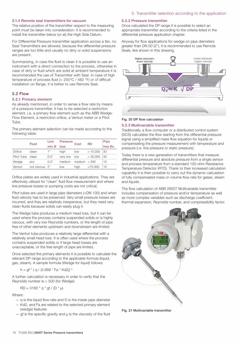
5.2.2 Pressure transmitter Once calculated the DP range it is possible to select an
appropriate transmitter according to the criteria listed in the
differential pressure application chapter.
Anyway for fl ow applications for wedge on pipe diameters
greater than DN 50 (2”), it is recommended to use Remote
Seals, like shown in this drawing.
Fig. 20 DP fl ow calculation
5.2.3 Multivariable transmitter Traditionally, a fl ow computer or a distributed control system
(DCS) calculates the fl ow starting from the differential pressure
signal using a simplifi ed mass fl ow equation for liquids or
compensating the pressure measurement with temperature and
pressure (i.e. line pressure or static pressure).
Today there is a new generation of transmitters that measure
differential pressure and absolute pressure from a single sensor
and process temperature from a standard 100-ohm Resistance
Temperature Detector (RTD). Thank to their increased calculation
capability it is then possible to carry out the dynamic calculation
of fully compensated mass or volume fl ow rate for gases, steam
and liquids.
The fl ow calculation of ABB 2600T Multivariable transmitter
includes compensation of pressure and/or temperature as well
as more complex variables such as discharge coeffi cient,
thermal expansion, Reynolds number, and compressibility factor.
Fig. 21 Multivariable transmitter
2600T Series Pressure transmitters | TI/266-EN 17
5. Transmitter selection according to the application
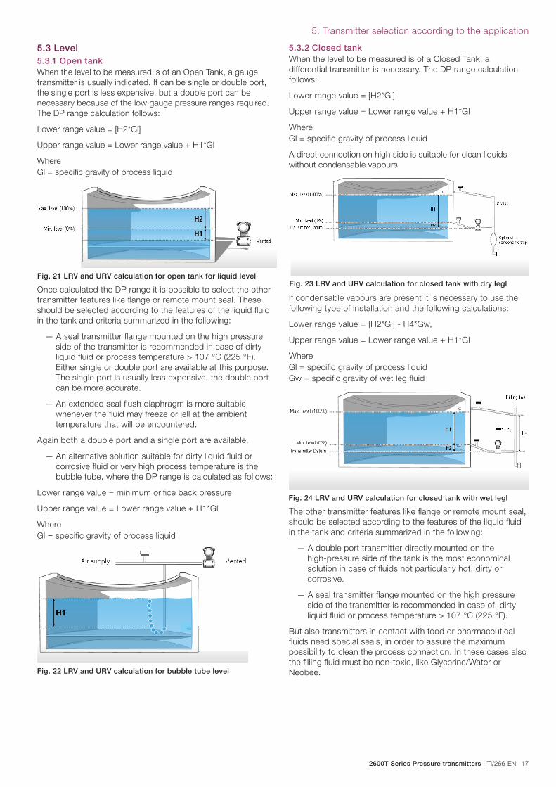
5.3 Level 5.3.1 Open tankWhen the level to be measured is of an Open Tank, a gauge
transmitter is usually indicated. It can be single or double port,
the single port is less expensive, but a double port can be
necessary because of the low gauge pressure ranges required.
The DP range calculation follows:
Lower range value = [H2*Gl]
Upper range value = Lower range value + H1*Gl
Where
Gl = specifi c gravity of process liquid
Fig. 21 LRV and URV calculation for open tank for liquid level
Once calculated the DP range it is possible to select the other
transmitter features like fl ange or remote mount seal. These
should be selected according to the features of the liquid fl uid
in the tank and criteria summarized in the following:
— A seal transmitter fl ange mounted on the high pressure
side of the transmitter is recommended in case of dirty
liquid fl uid or process temperature > 107 °C (225 °F).
Either single or double port are available at this purpose.
The single port is usually less expensive, the double port
can be more accurate.
— An extended seal fl ush diaphragm is more suitable
whenever the fl uid may freeze or jell at the ambient
temperature that will be encountered.
Again both a double port and a single port are available.
— An alternative solution suitable for dirty liquid fl uid or
corrosive fl uid or very high process temperature is the
bubble tube, where the DP range is calculated as follows:
Lower range value = minimum orifi ce back pressure
Upper range value = Lower range value + H1*Gl
Where
Gl = specifi c gravity of process liquid
Fig. 22 LRV and URV calculation for bubble tube level
5.3.2 Closed tankWhen the level to be measured is of a Closed Tank, a
differential transmitter is necessary. The DP range calculation
follows:
Lower range value = [H2*Gl]
Upper range value = Lower range value + H1*Gl
Where
Gl = specifi c gravity of process liquid
A direct connection on high side is suitable for clean liquids
without condensable vapours.
Fig. 23 LRV and URV calculation for closed tank with dry legl
If condensable vapours are present it is necessary to use the
following type of installation and the following calculations:
Lower range value = [H2*Gl] - H4*Gw,
Upper range value = Lower range value + H1*Gl
Where
Gl = specifi c gravity of process liquid
Gw = specifi c gravity of wet leg fl uid
Fig. 24 LRV and URV calculation for closed tank with wet legl
The other transmitter features like fl ange or remote mount seal,
should be selected according to the features of the liquid fl uid
in the tank and criteria summarized in the following:
— A double port transmitter directly mounted on the
high-pressure side of the tank is the most economical
solution in case of fl uids not particularly hot, dirty or
corrosive.
— A seal transmitter fl ange mounted on the high pressure
side of the transmitter is recommended in case of: dirty
liquid fl uid or process temperature > 107 °C (225 °F).
But also transmitters in contact with food or pharmaceutical
fl uids need special seals, in order to assure the maximum
possibility to clean the process connection. In these cases also
the fi lling fl uid must be non-toxic, like Glycerine/Water or
Neobee.
18 TI/266-EN | 2600T Series Pressure transmitters
5. Transmitter selection according to the application
Remote Seals are required also whenever:
— the process fl uid temperature is above 210 °C (410 °F) on
fl ange-mounted transmitters (and a cooling system is not
practical), or
— in case of long distances between the pressure taps of
differential pressure transmitter (up to 10 meter and in
some case even above), or
— to eliminate the need for seal pots, their installation and
maintenance, in particular for fl uids of the food/pharma
industry where seal pots cannot be utilized.
— An extended seal fl ush diaphragm in all of the above
cases is more suitable whenever the fl uid may freeze or jell
at the ambient temperature that will be encountered.
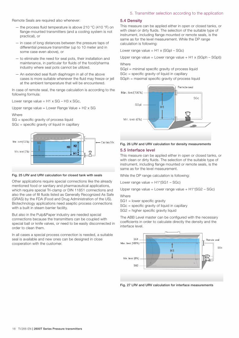
In case of remote seal, the range calculation is according to the
following formula:
Lower range value = H1 x SG – H3 x SGc,
Upper range value = Lower Range Value + H2 x SG
Where
SG = specifi c gravity of process liquid
SGc = specifi c gravity of liquid in capillary
Fig. 25 LRV and URV calculation for closed tank with seals
Other applications require special connections like the already
mentioned food or sanitary and pharmaceutical applications,
which require special Tri-clamp or DIN 11851 connections and
also the use of fi ll fl uids listed as Generally Recognized As Safe
(GRAS) by the FDA (Food and Drug Administration of the US).
Biotechnology applications need aseptic process connections
with a built in steam barrier facility.
But also in the Pulp&Paper industry are needed special
connections because the transmitters can be coupled with
special ball or knife valves, or need to be easily disconnected in
order to clean them.
In all cases a special process connection is needed, a suitable
seal is available and new ones can be designed in close
cooperation with the customer.
5.4 DensityThis measure can be applied either in open or closed tanks, or
with clean or dirty fl uids. The selection of the suitable type of
instrument, including fl ange mounted or remote seals, is the
same as for the level measurement. While the DP range
calculation is following:
Lower range value = H1 x (SGpl – SGc)
Upper range value = Lower range value + H1 x (SGph – SGpl))
Where
SGpl = minimal specifi c gravity of process liquid
SGc = specifi c gravity of liquid in capillary
SGph = maximal specifi c gravity of process liquid
Fig. 26 LRV and URV calculation for density measurements
5.5 Interface level This measure can be applied either in open or closed tanks, or
with clean or dirty fl uids. The selection of the suitable type of
instrument, including fl ange mounted or remote seals, is the
same as for the level measurement.
While the DP range calculation is following:
Lower range value = H1*(SG1 – SGc)
Upper range value = Lower range value + H1*(SG2 – SGc)
Where
SG1 = lower specifi c gravity
SGc = specifi c gravity of liquid in capillary
SG2 = higher specifi c gravity liquid
The ABB Level master can be confi gured with the necessary
coeffi cients in order to calculate directly the density and the
interface level.
Fig. 27 LRV and URV calculation for interface measurements
2600T Series Pressure transmitters | TI/266-EN 19
5. Transmitter selection according to the application
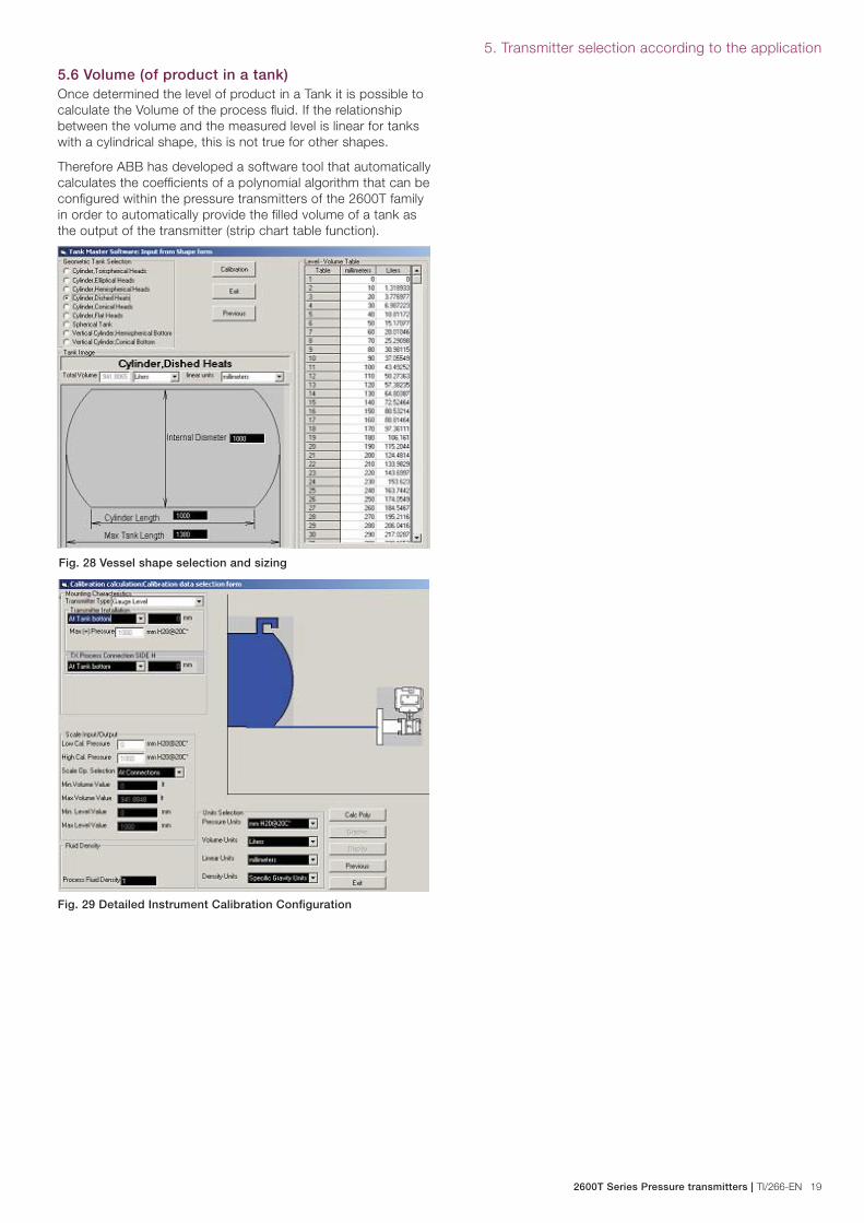
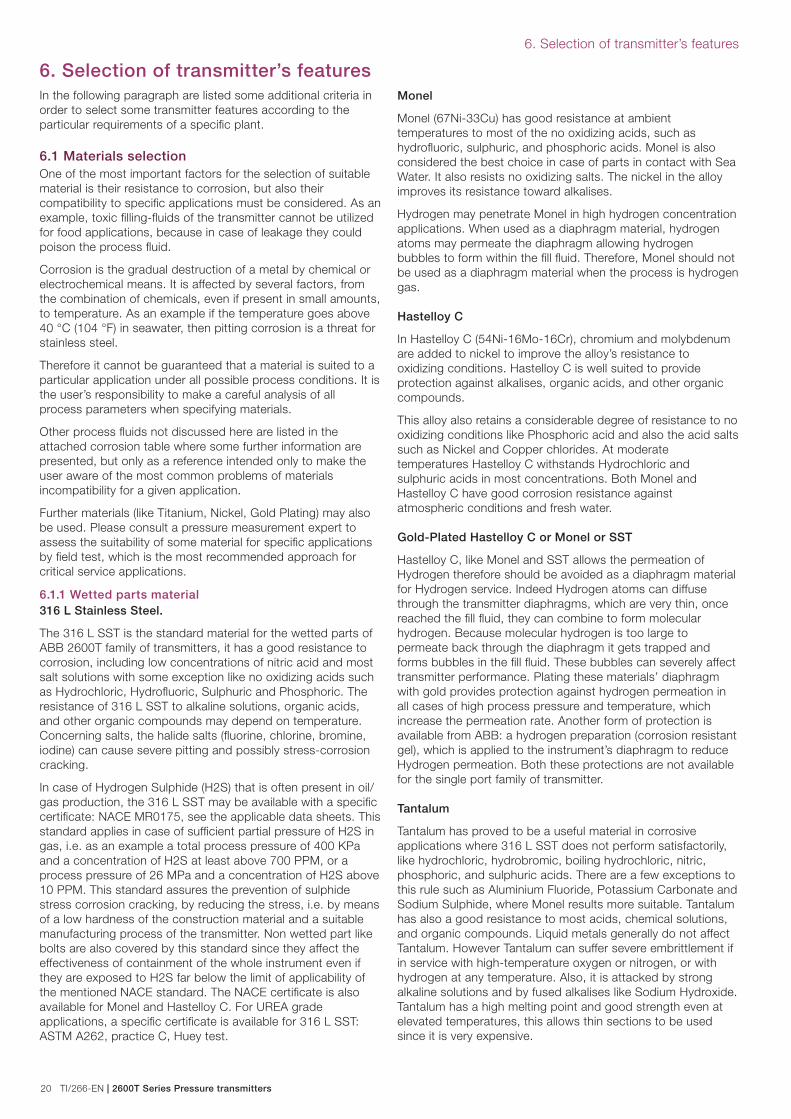
5.6 Volume (of product in a tank)Once determined the level of product in a Tank it is possible to
calculate the Volume of the process fl uid. If the relationship
between the volume and the measured level is linear for tanks
with a cylindrical shape, this is not true for other shapes.
Therefore ABB has developed a software tool that automatically
calculates the coeffi cients of a polynomial algorithm that can be
confi gured within the pressure transmitters of the 2600T family
in order to automatically provide the fi lled volume of a tank as
the output of the transmitter (strip chart table function).
Fig. 28 Vessel shape selection and sizing
Fig. 29 Detailed Instrument Calibration Confi guration
20 TI/266-EN | 2600T Series Pressure transmitters
6. Selection of transmitter’s features
6. Selection of transmitter’s featuresIn the following paragraph are listed some additional criteria in
order to select some transmitter features according to the
particular requirements of a specifi c plant.
6.1 Materials selectionOne of the most important factors for the selection of suitable
material is their resistance to corrosion, but also their
compatibility to specifi c applications must be considered. As an
example, toxic fi lling-fl uids of the transmitter cannot be utilized
for food applications, because in case of leakage they could
poison the process fl uid.
Corrosion is the gradual destruction of a metal by chemical or
electrochemical means. It is affected by several factors, from
the combination of chemicals, even if present in small amounts,
to temperature. As an example if the temperature goes above
40 °C (104 °F) in seawater, then pitting corrosion is a threat for
stainless steel.
Therefore it cannot be guaranteed that a material is suited to a
particular application under all possible process conditions. It is
the user’s responsibility to make a careful analysis of all
process parameters when specifying materials.
Other process fl uids not discussed here are listed in the
attached corrosion table where some further information are
presented, but only as a reference intended only to make the
user aware of the most common problems of materials
incompatibility for a given application.
Further materials (like Titanium, Nickel, Gold Plating) may also
be used. Please consult a pressure measurement expert to
assess the suitability of some material for specifi c applications
by fi eld test, which is the most recommended approach for
critical service applications.
6.1.1 Wetted parts material316 L Stainless Steel.
The 316 L SST is the standard material for the wetted parts of
ABB 2600T family of transmitters, it has a good resistance to
corrosion, including low concentrations of nitric acid and most
salt solutions with some exception like no oxidizing acids such
as Hydrochloric, Hydrofl uoric, Sulphuric and Phosphoric. The
resistance of 316 L SST to alkaline solutions, organic acids,
and other organic compounds may depend on temperature.
Concerning salts, the halide salts (fl uorine, chlorine, bromine,
iodine) can cause severe pitting and possibly stress-corrosion
cracking.
In case of Hydrogen Sulphide (H2S) that is often present in oil/
gas production, the 316 L SST may be available with a specifi c
certifi cate: NACE MR0175, see the applicable data sheets. This
standard applies in case of suffi cient partial pressure of H2S in
gas, i.e. as an example a total process pressure of 400 KPa
and a concentration of H2S at least above 700 PPM, or a
process pressure of 26 MPa and a concentration of H2S above
10 PPM. This standard assures the prevention of sulphide
stress corrosion cracking, by reducing the stress, i.e. by means
of a low hardness of the construction material and a suitable
manufacturing process of the transmitter. Non wetted part like
bolts are also covered by this standard since they affect the
effectiveness of containment of the whole instrument even if
they are exposed to H2S far below the limit of applicability of
the mentioned NACE standard. The NACE certifi cate is also
available for Monel and Hastelloy C. For UREA grade
applications, a specifi c certifi cate is available for 316 L SST:
ASTM A262, practice C, Huey test.
Monel
Monel (67Ni-33Cu) has good resistance at ambient
temperatures to most of the no oxidizing acids, such as
hydrofl uoric, sulphuric, and phosphoric acids. Monel is also
considered the best choice in case of parts in contact with Sea
Water. It also resists no oxidizing salts. The nickel in the alloy
improves its resistance toward alkalises.
Hydrogen may penetrate Monel in high hydrogen concentration
applications. When used as a diaphragm material, hydrogen
atoms may permeate the diaphragm allowing hydrogen
bubbles to form within the fi ll fl uid. Therefore, Monel should not
be used as a diaphragm material when the process is hydrogen
gas.
Hastelloy C
In Hastelloy C (54Ni-16Mo-16Cr), chromium and molybdenum
are added to nickel to improve the alloy’s resistance to
oxidizing conditions. Hastelloy C is well suited to provide
protection against alkalises, organic acids, and other organic
compounds.
This alloy also retains a considerable degree of resistance to no
oxidizing conditions like Phosphoric acid and also the acid salts
such as Nickel and Copper chlorides. At moderate
temperatures Hastelloy C withstands Hydrochloric and
sulphuric acids in most concentrations. Both Monel and
Hastelloy C have good corrosion resistance against
atmospheric conditions and fresh water.
Gold-Plated Hastelloy C or Monel or SST
Hastelloy C, like Monel and SST allows the permeation of
Hydrogen therefore should be avoided as a diaphragm material
for Hydrogen service. Indeed Hydrogen atoms can diffuse
through the transmitter diaphragms, which are very thin, once
reached the fi ll fl uid, they can combine to form molecular
hydrogen. Because molecular hydrogen is too large to
permeate back through the diaphragm it gets trapped and
forms bubbles in the fi ll fl uid. These bubbles can severely affect
transmitter performance. Plating these materials’ diaphragm
with gold provides protection against hydrogen permeation in
all cases of high process pressure and temperature, which
increase the permeation rate. Another form of protection is
available from ABB: a hydrogen preparation (corrosion resistant
gel), which is applied to the instrument’s diaphragm to reduce
Hydrogen permeation. Both these protections are not available
for the single port family of transmitter.
Tantalum
Tantalum has proved to be a useful material in corrosive
applications where 316 L SST does not perform satisfactorily,
like hydrochloric, hydrobromic, boiling hydrochloric, nitric,
phosphoric, and sulphuric acids. There are a few exceptions to
this rule such as Aluminium Fluoride, Potassium Carbonate and
Sodium Sulphide, where Monel results more suitable. Tantalum
has also a good resistance to most acids, chemical solutions,
and organic compounds. Liquid metals generally do not affect
Tantalum. However Tantalum can suffer severe embrittlement if
in service with high-temperature oxygen or nitrogen, or with
hydrogen at any temperature. Also, it is attacked by strong
alkaline solutions and by fused alkalises like Sodium Hydroxide.
Tantalum has a high melting point and good strength even at
elevated temperatures, this allows thin sections to be used
since it is very expensive.
2600T Series Pressure transmitters | TI/266-EN 21
6. Selection of transmitter’s features
PFA (Tefl on from Dupont)
ABB offers another unique solution to corrosive application. It
consists of a PFA (Tefl on) coating of an AISI 316 L SS remote
seal transmitter. The PFA corrosion suitability is really
outstanding and a coating of 0,2-0,3 mm can solve severe
corrosion application in a cost-effective way, i.e. without
recurring to the use of more expensive metals.
The only limitation is the recommended process temperature of
200 °C (392 °F) and a minimum increase of the temperature
effect on accuracy.
6.1.2 HousingFor marine environment there is a corrosion risk, related to the
presence of chloride, an ion that gives place to an accelerated
galvanic corrosion of aluminium housing because of the copper
content of aluminium alloy. ABB transmitter housings are
copper free (copper content of aluminium less than 0,03 %).
6.1.3 Fill fluidThe type of fi ll fl uid selected can limit the working temperature
that the transmitter can stand. Therefore the fi ll fl uid shall be
selected on the fl uid table according to the applicable
temperature. This temperature can be considered the ambient
one, because even with higher process temperature, this
sharply decreases along the piping connection to the
transmitter.
The most utilized fi ll fl uid is Silicone Oil DC200 because of its
high stability over a wide range of operating temperatures:
-40 °C to 200 °C (-40 °F to 392 °F). Other fl uids may be
selected, whenever their temperature range is compatible with
the application, in order to take advantage of a lower viscosity
or a lower thermal expansion factor. In particular this could be
very useful to improve the response time in case of remote seal
application with long capillaries. For some food or
pharmaceutical application the fi ll fl uid must not to be toxic in
order to prevent problems in case of diaphragm rupture and
product contamination. In this case a food sanitary fi ll fl uid shall
be selected. Another special case that impacts the fi ll fl uid is
the application of a transmitter on Oxygen service, since
Siliconee oil could fi re in case of fl uid losses, an inert fl uid shall
be selected.
6.1.4 GasketThe most widespread material for the transmitter gasket is
PTFE (Tefl on) because of its general corrosion suitability with
several materials. A known limitation is in case of process
which temperature can periodically vary of several degrees,
compromising the tightness because of the limited elasticity of
this material. In these cases special materials may be asked to
local ABB representatives.
Other special cases are the food or pharmaceutical applications
that require an approved material listed by the American Food
and Drug Administration (FDA) or other national equivalent
bodies.
6.2 Overpressure limitsThe maximum pressure that a transmitter can withstand
without damages (i.e. no recalibration is required) is called
Overpressure. For Differential Pressure transmitter, the
overpressure is also called Static Pressure and is usually
applied to both side of the transmitter (High and Low). This
pressure depends on the mechanical features of the transmitter
and in particular on the type of sensor and of process fl anges.
Sensors suitable for low ranges of pressure can stand lower
overpressure.
The standard Maximum Withstanded Pressure (MWP) of a
pressure transmitter is of 21 MPa, but it may differ according to
the sensor selected. In case of higher process pressure
requirements, use specifi c versions of sensors and process
connections (the latter in combination with temperature) with an
overpressure limit of 60 MPa, 8700 psi (these models are called
“High Static”).
The exposure of a transmitter to a very high pressure, above
the maximum operating pressure rating, can lead to a
mechanical modifi cation of the diaphragm, or to leakage or
even a dangerous rupture (resulting in fl ying fragments outside
the device). The capability of the transmitter to avoid leakage
and dangerous rupture is certifi ed according to the SAMA PMC
27.1 standard at a pressure of 48 MPa (6960 psi), 90 MPa
(13054 psi) for High Static models.
In order to identify the real overpressure limit requirement, it is
usually enough to check the conditions at the border of the
application, some example are provided in the following:
closed vessel
— maximum pressure of the lines connected (fi lling fl uids or
inert gas),
— refl ux from downstream equipment
— max pressure generated from a chemical reaction
Pipeline
— design rating of the line (to be checked on the P&ID if
available)
— max prevalence of the upstream pump
6.3 Temperature limitsMost electronic transmitters are rated for operation at ambient
temperature from as low as – 20 ° to – 40 °C (– 4 ° to – 40 °F)
to a high temperature between 60° to 85°C (140 ° to 185 °F),
depending on the fi lling materials that are used within the
transmitter.
However the ambient temperature fl uctuations has also to be
carefully considered. For example, consider a transmitter that is
installed in a measurement loop and which is located outdoors
in an unprotected location where it receives sunlight from
9:00 AM to 4:00 PM. The transmitter output, will most likely
show some zero shift during the hours of sunlight, even when
the air temperature is constant. The zero shift is caused by an
increase of the internal temperature of the transmitter due to
the radiant heat effect of the sun. A sudden rain shower, or a
strong cooling wind could have similar effects on the
transmitter output. Furthermore high temperatures accelerate
any degradation of electrical components, so high temperature
(above 60 °C, 140 °F) should be avoided whenever practical.
6.4 AccuracyFor the ABB 2600 T family of transmitter there is the possibility
to select among various base accuracy from 0,025% to 0,10%.
This depends on the application requirements.
As an example the highest accuracy may be required for fl ow
measurement and totalisation for transfer or fi scal metering.
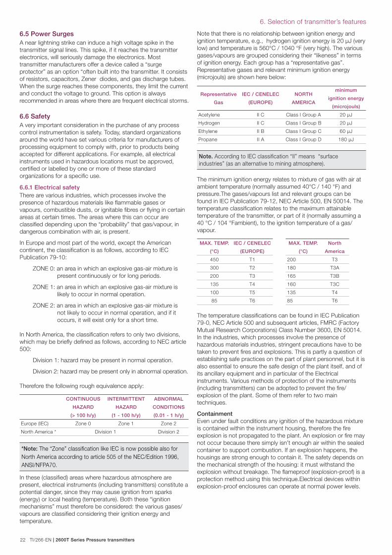
22 TI/266-EN | 2600T Series Pressure transmitters
6. Selection of transmitter’s features
6.5 Power SurgesA near lightning strike can induce a high voltage spike in the
transmitter signal lines. This spike, if it reaches the transmitter
electronics, will seriously damage the electronics. Most
transmitter manufacturers offer a device called a “surge
protector” as an option “often built into the transmitter. It consists
of resistors, capacitors, Zener diodes, and gas discharge tubes.
When the surge reaches these components, they limit the current
and conduct the voltage to ground. This option is always
recommended in areas where there are frequent electrical storms.
6.6 SafetyA very important consideration in the purchase of any process
control instrumentation is safety. Today, standard organizations
around the world have set various criteria for manufacturers of
processing equipment to comply with, prior to products being
accepted for different applications. For example, all electrical
instruments used in hazardous locations must be approved,
certifi ed or labelled by one or more of these standard
organizations for a specifi c use.
6.6.1 Electrical safetyThere are various industries, which processes involve the
presence of hazardous materials like fl ammable gases or
vapours, combustible dusts, or ignitable fi bres or fl ying in certain
areas at certain times. The areas where this can occur are
classifi ed depending upon the “probability” that gas/vapour, in
dangerous combination with air, is present.
In Europe and most part of the world, except the American
continent, the classifi cation is as follows, according to IEC
Publication 79-10:
ZONE 0: an area in which an explosive gas-air mixture is
present continuously or for long periods.
ZONE 1: an area in which an explosive gas-air mixture is
likely to occur in normal operation.
ZONE 2: an area in which an explosive gas-air mixture is
not likely to occur in normal operation, and if it
occurs, it will exist only for a short time.
In North America, the classifi cation refers to only two divisions,
which may be briefl y defi ned as follows, according to NEC article
500:
Division 1: hazard may be present in normal operation.
Division 2: hazard may be present only in abnormal operation.
Therefore the following rough equivalence apply:
CONTINUOUS
HAZARD
(> 100 h/y)
INTERMITTENT
HAZARD
(1 - 100 h/y)
ABNORMAL
CONDITIONS
(0.01 - 1 h/y)
Europe (IEC) Zone 0 Zone 1 Zone 2
North America * Division 1 Division 2
*Note: The “Zone” classifi cation like IEC is now possible also for
North America according to article 505 of the NEC/Edition 1996,
ANSI/NFPA70.
In these (classifi ed) areas where hazardous atmosphere are
present, electrical instruments (including transmitters) constitute a
potential danger, since they may cause ignition from sparks
(energy) or local heating (temperature). Both these “ignition
mechanisms” must therefore be considered: the various gases/
vapours are classifi ed considering their ignition energy and
temperature.
Note that there is no relationship between ignition energy and
ignition temperature, e.g., hydrogen ignition energy is 20 µJ (very
low) and temperature is 560°C / 1040 °F (very high). The various
gases/vapours are grouped considering their “likeness” in terms
of ignition energy. Each group has a “representative gas”.
Representative gases and relevant minimum ignition energy
(microjouls) are shown here below:
Representative
Gas
IEC / CENELEC
(EUROPE)
NORTH
AMERICA
minimum
ignition energy
(microjouls)
Acetylene II C Class I Group A 20 µJ
Hydrogen II C Class I Group B 20 µJ
Ethylene II B Class I Group C 60 µJ
Propane II A Class I Group D 180 µJ
Note. According to IEC classifi cation “II” means “surface
industries” (as an alternative to mining atmosphere).
The minimum ignition energy relates to mixture of gas with air at
ambient temperature (normally assumed 40°C / 140 °F) and
pressure.The gases/vapours list and relevant groups can be
found in IEC Publication 79-12, NEC Article 500, EN 50014. The
temperature classifi cation relates to the maximum attainable
temperature of the transmitter, or part of it (normally assuming a
40 °C / 104 °Fambient), to the ignition temperature of a gas/
vapour.
MAX. TEMP.
(°C)
IEC / CENELEC
(EUROPE)
450 T1
300 T2
200 T3
135 T4
100 T5
85 T6
MAX. TEMP.
(°C)
North
America
200 T3
180 T3A
165 T3B
160 T3C
135 T4
85 T6
The temperature classifi cations can be found in IEC Publication
79-0, NEC Article 500 and subsequent articles, FMRC (Factory
Mutual Research Corporations) Class Number 3600, EN 50014.
In the industries, which processes involve the presence of
hazardous materials industries, stringent precautions have to be
taken to prevent fi res and explosions. This is partly a question of
establishing safe practices on the part of plant personnel, but it is
also essential to ensure the safe design of the plant itself, and of
its ancillary equipment and in particular of the Electrical
instruments. Various methods of protection of the instruments
(including transmitters) can be adopted to prevent the fi re/
explosion of the plant. Some of them refer to two main
techniques.
Containment Even under fault conditions any ignition of the hazardous mixture
is contained within the instrument housing, therefore the fi re
explosion is not propagated to the plant. An explosion or fi re may
not occur because there simply isn’t enough air within the sealed
container to support combustion. If an explosion happens, the
housings are strong enough to contain it. The safety depends on
the mechanical strength of the housing: it must withstand the
explosion without breakage. The fl ameproof (explosion-proof) is a
protection method using this technique.Electrical devices within
explosion-proof enclosures can operate at normal power levels.
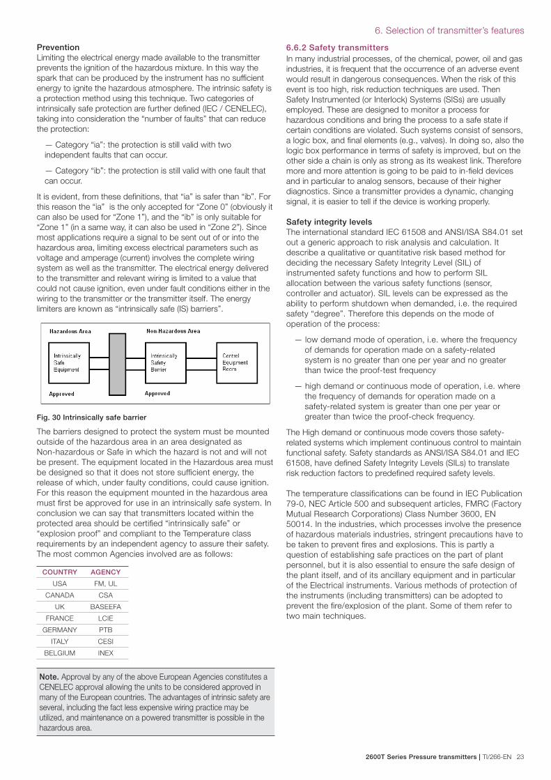
2600T Series Pressure transmitters | TI/266-EN 23
6. Selection of transmitter’s features
Prevention
Limiting the electrical energy made available to the transmitter
prevents the ignition of the hazardous mixture. In this way the
spark that can be produced by the instrument has no suffi cient
energy to ignite the hazardous atmosphere. The intrinsic safety is
a protection method using this technique. Two categories of
intrinsically safe protection are further defi ned (IEC / CENELEC),
taking into consideration the “number of faults” that can reduce
the protection:
— Category “ia”: the protection is still valid with two
independent faults that can occur.
— Category “ib”: the protection is still valid with one fault that
can occur.
It is evident, from these defi nitions, that “ia” is safer than “ib”. For
this reason the “ia” is the only accepted for “Zone 0” (obviously it
can also be used for “Zone 1”), and the “ib” is only suitable for
“Zone 1” (in a same way, it can also be used in “Zone 2”). Since
most applications require a signal to be sent out of or into the
hazardous area, limiting excess electrical parameters such as
voltage and amperage (current) involves the complete wiring
system as well as the transmitter. The electrical energy delivered
to the transmitter and relevant wiring is limited to a value that
could not cause ignition, even under fault conditions either in the
wiring to the transmitter or the transmitter itself. The energy
limiters are known as “intrinsically safe (IS) barriers”.
Fig. 30 Intrinsically safe barrier
The barriers designed to protect the system must be mounted
outside of the hazardous area in an area designated as
Non-hazardous or Safe in which the hazard is not and will not
be present. The equipment located in the Hazardous area must
be designed so that it does not store suffi cient energy, the
release of which, under faulty conditions, could cause ignition.
For this reason the equipment mounted in the hazardous area
must fi rst be approved for use in an intrinsically safe system. In
conclusion we can say that transmitters located within the
protected area should be certifi ed “intrinsically safe” or
“explosion proof” and compliant to the Temperature class
requirements by an independent agency to assure their safety.
The most common Agencies involved are as follows:
COUNTRY AGENCY
USA FM, UL
CANADA CSA
UK BASEEFA
FRANCE LCIE
GERMANY PTB
ITALY CESI
BELGIUM INEX
Note. Approval by any of the above European Agencies constitutes a
CENELEC approval allowing the units to be considered approved in
many of the European countries. The advantages of intrinsic safety are
several, including the fact less expensive wiring practice may be
utilized, and maintenance on a powered transmitter is possible in the
hazardous area.
6.6.2 Safety transmittersIn many industrial processes, of the chemical, power, oil and gas
industries, it is frequent that the occurrence of an adverse event
would result in dangerous consequences. When the risk of this
event is too high, risk reduction techniques are used. Then
Safety Instrumented (or Interlock) Systems (SISs) are usually
employed. These are designed to monitor a process for
hazardous conditions and bring the process to a safe state if
certain conditions are violated. Such systems consist of sensors,
a logic box, and fi nal elements (e.g., valves). In doing so, also the
logic box performance in terms of safety is improved, but on the
other side a chain is only as strong as its weakest link. Therefore
more and more attention is going to be paid to in-fi eld devices
and in particular to analog sensors, because of their higher
diagnostics. Since a transmitter provides a dynamic, changing
signal, it is easier to tell if the device is working properly.
Safety integrity levels
The international standard IEC 61508 and ANSI/ISA S84.01 set
out a generic approach to risk analysis and calculation. It
describe a qualitative or quantitative risk based method for
deciding the necessary Safety Integrity Level (SIL) of
instrumented safety functions and how to perform SIL
allocation between the various safety functions (sensor,
controller and actuator). SIL levels can be expressed as the
ability to perform shutdown when demanded, i.e. the required
safety “degree”. Therefore this depends on the mode of
operation of the process:
— low demand mode of operation, i.e. where the frequency
of demands for operation made on a safety-related
system is no greater than one per year and no greater
than twice the proof-test frequency
— high demand or continuous mode of operation, i.e. where
the frequency of demands for operation made on a
safety-related system is greater than one per year or
greater than twice the proof-check frequency.
The High demand or continuous mode covers those safety-
related systems which implement continuous control to maintain
functional safety. Safety standards as ANSI/ISA S84.01 and IEC
61508, have defi ned Safety Integrity Levels (SILs) to translate
risk reduction factors to predefi ned required safety levels.
The temperature classifi cations can be found in IEC Publication
79-0, NEC Article 500 and subsequent articles, FMRC (Factory
Mutual Research Corporations) Class Number 3600, EN
50014. In the industries, which processes involve the presence
of hazardous materials industries, stringent precautions have to
be taken to prevent fi res and explosions. This is partly a
question of establishing safe practices on the part of plant
personnel, but it is also essential to ensure the safe design of
the plant itself, and of its ancillary equipment and in particular
of the Electrical instruments. Various methods of protection of
the instruments (including transmitters) can be adopted to
prevent the fi re/explosion of the plant. Some of them refer to
two main techniques.
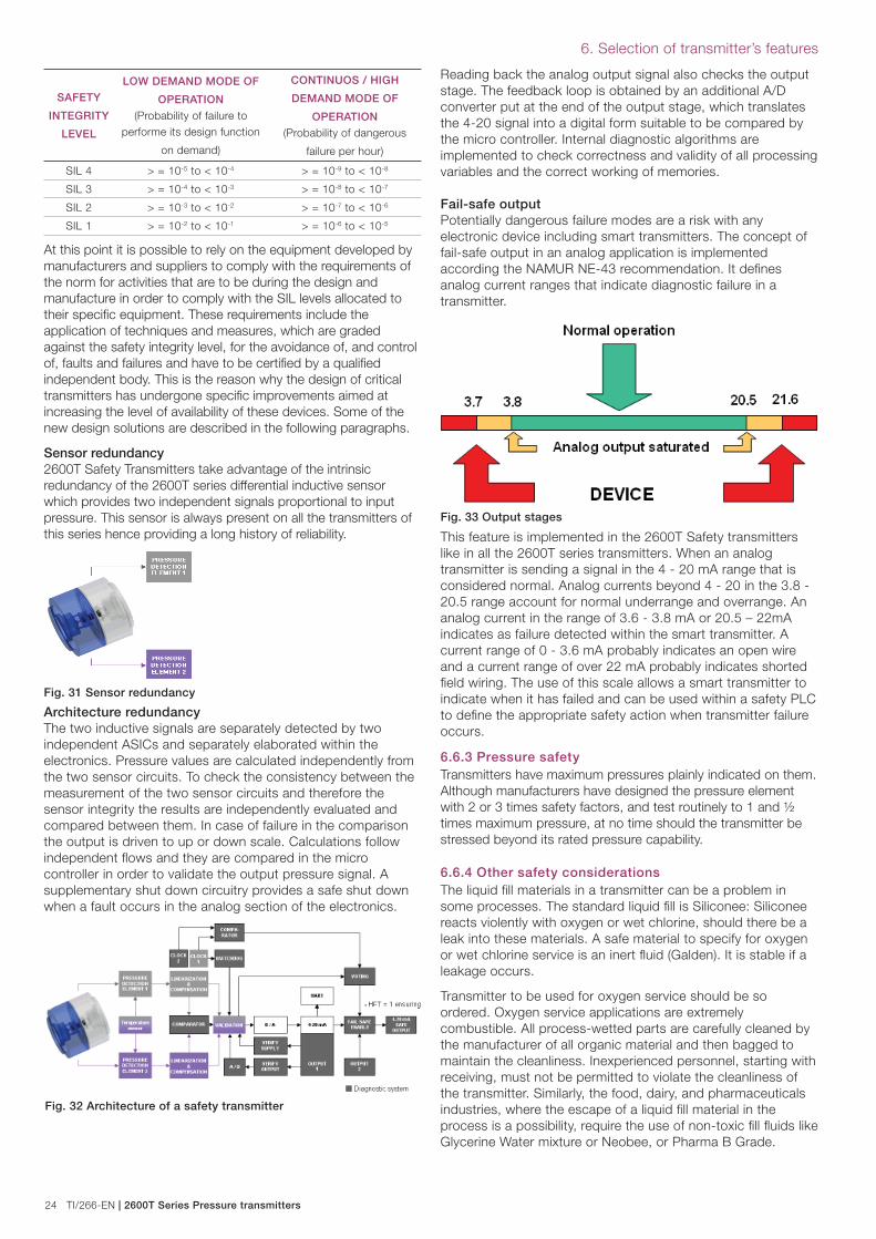
24 TI/266-EN | 2600T Series Pressure transmitters
6. Selection of transmitter’s features
SAFETY
INTEGRITY
LEVEL
LOW DEMAND MODE OF
OPERATION
(Probability of failure to
performe its design function
on demand)
CONTINUOS / HIGH
DEMAND MODE OF
OPERATION
(Probability of dangerous
failure per hour)
SIL 4 > = 10-5 to < 10-4 > = 10-9 to < 10-8
SIL 3 > = 10-4 to < 10-3 > = 10-8 to < 10-7
SIL 2 > = 10-3 to < 10-2 > = 10-7 to < 10-6
SIL 1 > = 10-2 to < 10-1 > = 10-6 to < 10-5
At this point it is possible to rely on the equipment developed by
manufacturers and suppliers to comply with the requirements of
the norm for activities that are to be during the design and
manufacture in order to comply with the SIL levels allocated to
their specifi c equipment. These requirements include the
application of techniques and measures, which are graded
against the safety integrity level, for the avoidance of, and control
of, faults and failures and have to be certifi ed by a qualifi ed
independent body. This is the reason why the design of critical
transmitters has undergone specifi c improvements aimed at
increasing the level of availability of these devices. Some of the
new design solutions are described in the following paragraphs.
Sensor redundancy
2600T Safety Transmitters take advantage of the intrinsic
redundancy of the 2600T series differential inductive sensor
which provides two independent signals proportional to input
pressure. This sensor is always present on all the transmitters of
this series hence providing a long history of reliability.
Fig. 31 Sensor redundancy
Architecture redundancy The two inductive signals are separately detected by two
independent ASICs and separately elaborated within the
electronics. Pressure values are calculated independently from
the two sensor circuits. To check the consistency between the
measurement of the two sensor circuits and therefore the
sensor integrity the results are independently evaluated and
compared between them. In case of failure in the comparison
the output is driven to up or down scale. Calculations follow
independent fl ows and they are compared in the micro
controller in order to validate the output pressure signal. A
supplementary shut down circuitry provides a safe shut down
when a fault occurs in the analog section of the electronics.
Reading back the analog output signal also checks the output
stage. The feedback loop is obtained by an additional A/D
converter put at the end of the output stage, which translates
the 4-20 signal into a digital form suitable to be compared by
the micro controller. Internal diagnostic algorithms are
implemented to check correctness and validity of all processing
variables and the correct working of memories.
Fail-safe output Potentially dangerous failure modes are a risk with any
electronic device including smart transmitters. The concept of
fail-safe output in an analog application is implemented
according the NAMUR NE-43 recommendation. It defi nes
analog current ranges that indicate diagnostic failure in a
transmitter.
Fig. 33 Output stages
This feature is implemented in the 2600T Safety transmitters
like in all the 2600T series transmitters. When an analog
transmitter is sending a signal in the 4 - 20 mA range that is
considered normal. Analog currents beyond 4 - 20 in the 3.8 -
20.5 range account for normal underrange and overrange. An
analog current in the range of 3.6 - 3.8 mA or 20.5 – 22mA
indicates as failure detected within the smart transmitter. A
current range of 0 - 3.6 mA probably indicates an open wire
and a current range of over 22 mA probably indicates shorted
fi eld wiring. The use of this scale allows a smart transmitter to
indicate when it has failed and can be used within a safety PLC
to defi ne the appropriate safety action when transmitter failure
occurs.
6.6.3 Pressure safetyTransmitters have maximum pressures plainly indicated on them.
Although manufacturers have designed the pressure element
with 2 or 3 times safety factors, and test routinely to 1 and ½
times maximum pressure, at no time should the transmitter be
stressed beyond its rated pressure capability.
6.6.4 Other safety considerationsThe liquid fi ll materials in a transmitter can be a problem in
some processes. The standard liquid fi ll is Siliconee: Siliconee
reacts violently with oxygen or wet chlorine, should there be a
leak into these materials. A safe material to specify for oxygen
or wet chlorine service is an inert fl uid (Galden). It is stable if a
leakage occurs.
Transmitter to be used for oxygen service should be so
ordered. Oxygen service applications are extremely
combustible. All process-wetted parts are carefully cleaned by
the manufacturer of all organic material and then bagged to
maintain the cleanliness. Inexperienced personnel, starting with
receiving, must not be permitted to violate the cleanliness of
the transmitter. Similarly, the food, dairy, and pharmaceuticals
industries, where the escape of a liquid fi ll material in the
process is a possibility, require the use of non-toxic fi ll fl uids like
Glycerine Water mixture or Neobee, or Pharma B Grade.
Fig. 32 Architecture of a safety transmitter
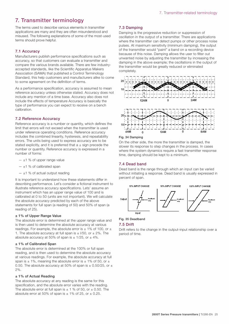
2600T Series Pressure transmitters | TI/266-EN 25
7. Transmitter-related terminology
7. Transmitter terminologyThe terms used to describe various elements in transmitter
applications are many and they are often misunderstood and
misused. The following explanations of some of the most-used
terms should prove helpful.
7.1 AccuracyManufacturers publish performance specifi cations such as
accuracy, so that customers can evaluate a transmitter and
compare the various brands available. There are few industry-
accepted standards, like the Scientifi c Apparatus Makers
Association (SAMA) that published a Control Terminology
Standard, this help customers and manufacturers alike to come
to some agreement on the defi nition of terms.
As a performance specifi cation, accuracy is assumed to mean
reference accuracy unless otherwise stated. Accuracy does not
include any mention of a time base. Accuracy also does not
include the effects of temperature Accuracy is basically the
type of performance you can expect to receive on a bench
calibration.
7.2 Reference AccuracyReference accuracy is a number or quantity, which defi nes the
limit that errors will not exceed when the transmitter is used
under reference operating conditions. Reference accuracy
includes the combined linearity, hysteresis, and repeatability
errors. The units being used to express accuracy are to be
stated explicitly, and it is preferred that a ± sign precede the
number or quantity. Reference accuracy is expressed in a
number of forms:
— ±1 % of upper range value
— ±1 % of calibrated span
— ±1 % of actual output reading
It is important to understand how these statements differ in
describing performance. Let’s consider a fi ctional instrument to
illustrate reference accuracy specifi cations. Lets’ assume an
instrument which has an upper range value of 100 and is
calibrated at 0 to 50 (units are not important). We will calculate
the absolute accuracy predicted by each of the above
statements for full span (a reading of 50) and 50% of span (a
reading of 25).
± 1% of Upper Range Value The absolute error is determined at the upper range value and
is then used to determine the absolute accuracy at various
readings. For example, the absolute error is ± 1% of 100, or ±
1. The absolute accuracy at full span is ± l/50, or ± 2%. The
absolute accuracy at 50% of span is ± 1/25, or ± 4%.
± 1% of Calibrated Span
The absolute error is determined at the 100% or full span
reading, and is then used to determine the absolute accuracy
at various readings. For example, the absolute accuracy at full
span is ± 1%, meaning the absolute error is ± 1% of 50, or ±
0.50. The absolute accuracy at 50% of span is ± 0.50/25, or ±
2%.
± 1% of Actual Reading
The absolute accuracy at any reading is the same for this
specifi cation, and the absolute error varies with the reading.
The absolute error at full span is ± 1 % of 50, or ± 0.50. The
absolute error at 50% of span is ± 1% of 25, or ± 0.25.
7.3 Damping Damping is the progressive reduction or suppression of
oscillation in the output of a transmitter. There are applications
where the transmitter can detect pumps or other process noise
pulses. At maximum sensitivity (minimum damping), the output
of the transmitter would “paint” a band on a recording device
because of this noise. Damping allows the user to fi lter out
unwanted noise by adjusting the transmitter by increasing the
damping in the above example; the oscillations in the output of
the transmitter would be greatly reduced or eliminated
completely.
Fig. 34 Damping
On the other side, the more the transmitter is damped, the
slower its response to step changes in the process. In cases
where the system dynamics require a fast transmitter response
time, damping should be kept to a minimum.
7.4 Dead bandDead band is the range through which an input can be varied
without initiating a response. Dead band is usually expressed in
percent of span.
Fig. 35 Deadband
7.5 DriftDrift refers to the change in the output-input relationship over a
period of time.
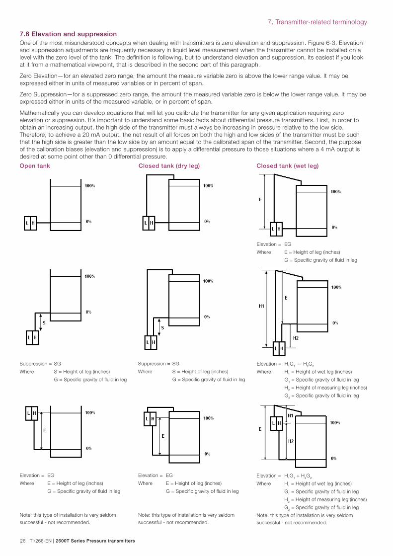
26 TI/266-EN | 2600T Series Pressure transmitters
7. Transmitter-related terminology
7.6 Elevation and suppression One of the most misunderstood concepts when dealing with transmitters is zero elevation and suppression. Figure 6-3. Elevation
and suppression adjustments are frequently necessary in liquid level measurement when the transmitter cannot be installed on a
level with the zero level of the tank. The defi nition is following, but to understand elevation and suppression, its easiest if you look
at it from a mathematical viewpoint, that is described in the second part of this paragraph.
Zero Elevation—for an elevated zero range, the amount the measure variable zero is above the lower range value. It may be
expressed either in units of measured variables or in percent of span.
Zero Suppression—for a suppressed zero range, the amount the measured variable zero is below the lower range value. It may be
expressed either in units of the measured variable, or in percent of span.
Mathematically you can develop equations that will let you calibrate the transmitter for any given application requiring zero
elevation or suppression. It’s important to understand some basic facts about differential pressure transmitters. First, in order to
obtain an increasing output, the high side of the transmitter must always be increasing in pressure relative to the low side.
Therefore, to achieve a 20 mA output, the net result of all forces on both the high and low sides of the transmitter must be such
that the high side is greater than the low side by an amount equal to the calibrated span of the transmitter. Second, the purpose
of the calibration biases (elevation and suppression) is to apply a differential pressure to those situations where a 4 mA output is
desired at some point other than 0 differential pressure.
Open tank
Elevation = EG
Where E = Height of leg (inches)
G = Specifi c gravity of fl uid in leg
Suppression = SG
Where S = Height of leg (inches)
G = Specifi c gravity of fl uid in leg
Closed tank (dry leg) Closed tank (wet leg)
Elevation = EG
Where E = Height of leg (inches)
G = Specifi c gravity of fl uid in leg
Note: this type of installation is very seldom
successful - not recommended.
Suppression = SG
Where S = Height of leg (inches)
G = Specifi c gravity of fl uid in leg
Elevation = H1G
1 — H
2G
2
Where H1 = Height of wet leg (inches)
G1 = Specifi c gravity of fl uid in leg
H2 = Height of measuring leg (inches)
G2 = Specifi c gravity of fl uid in leg
Elevation = EG
Where E = Height of leg (inches)
G = Specifi c gravity of fl uid in leg
Note: this type of installation is very seldom
successful - not recommended.
Elevation = H1G
1 + H
2G
2
Where H1 = Height of wet leg (inches)
G1 = Specifi c gravity of fl uid in leg
H2 = Height of measuring leg (inches)
G2 = Specifi c gravity of fl uid in leg
Note: this type of installation is very seldom
successful - not recommended.
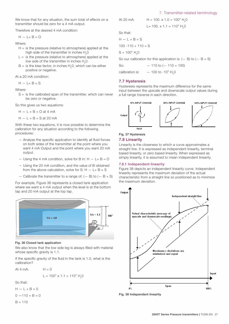
2600T Series Pressure transmitters | TI/266-EN 27
7. Transmitter-related terminology
We know that for any situation, the sum total of effects on a
transmitter should be zero for a 4 mA output.
Therefore at the desired 4 mA condition:
H — L+ B = O
Where:
H = is the pressure (relative to atmosphere) applied at the
high side of the transmitter in inches H20
L = is the pressure (relative to atmosphere) applied at the
low side of the transmitter in inches H20.
B = is the bias factor, in inches H20, which can be either
positive or negative.
At a 20 mA condition:
H — L+ B = S
Where:
S = is the calibrated span of the transmitter, which can never
be zero or negative.
So this gives us two equations:
H — L + B = O at 4 mA
H — L + B = S at 20 mA
With these two equations, it is now possible to determine the
calibration for any situation according to the following
procedures:
— Analyse the specifi c application to identify all fl uid forces
on both sides of the transmitter at the point where you
want 4 mA Output and the point where you want 20 mA
output.
— Using the 4 mA condition, solve for B in: H — L+ B = O
— Using the 20 mA condition, and the value of B obtained
from the above calculation, solve for S: H — L+ B = S
— Calibrate the transmitter to a range of: (— B) to (— B + S)
For example, Figure 36 represents a closed tank application
where we want a 4 mA output when the level is at the bottom
tap and 20 mA output at the top tap.
We also know that the low side leg is always fi lled with material
whose specifi c gravity is 1.1.
If the specifi c gravity of the fl uid in the tank is 1.0, what is the
calibration?
At 4 mA: H = 0
L = 100” x 1.1 = 110” H20
So that:
H — L + B = 0
0 —110 + B = 0
B = 110
Fig. 36 Closed tank application
At 20 mA: H = 100. x 1.0 = 100” H20
L= 100. x 1.1 = 110” H20
So that:
H — L + B = S
100 -110 + 110 = S
S = 100” H20
So our calibration for this application is: (— B) to (— B + S)
So: — 110 to (— 110 + 100)
calibration is: — 100 to -10” H20
7.7 HysteresisHysteresis represents the maximum difference for the same
input between the upscale and downscale output values during
a full range traverse in each direction.
Fig. 37 Hysteresis
7.8 LinearityLinearity is the closeness to which a curve approximates a
straight line. It is expressed as independent linearity, terminal
based linearity, or zero based linearity. When expressed as
simply linearity, it is assumed to mean independent linearity.
7.8.1 Independent linearity Figure 38 depicts an independent linearity curve. Independent
linearity represents the maximum deviation of the actual
characteristic from a straight line so positioned as to minimize
the maximum deviation.
Fig. 38 Independent linearity

28 TI/266-EN | 2600T Series Pressure transmitters
7. Transmitter-related terminology
7.8.2 Terminal-based linearity Terminal based linearity, Figure 39, is the maximum deviation of
the actual characteristics from a straight line coinciding with the
actual characteristic at upper and lower range values.
Fig. 39 Terminal-based linearity
7.8.3 Zero-based linearity The maximum deviation of the actual characteristic from a
straight line so positioned as to coincide with the actual
characteristic at the lower range value and to minimize
maximum deviation is referred to as zero based linearity.
Fig. 39 Zero-based linearity
7.9 Maximum Withstanded Pressure (MWP) See Overpressure
7.10 Output The standard output for a two-wire transmitter is 4-20 mA dc.
7.11 Pressure7.11.1 Pressure definition from physicPressure is force distributed over, a surface. The pressure P of
a force F distributed over an area A is defi ned as:
P = FA
7.11.2 Atmospheric pressureThe pressure exerted by the earth’s atmosphere. Atmospheric
pressure at sea level is about 100 KPa or 1 Bar or 15 psi.
The value of atmospheric pressure decreases with increasing
altitude.
7.11.3 OverpressureIt is the maximum pressure withstanded without damage by the
transmitter. It is also indicated as Maximum Withstanded
Pressure (MWP). See also the relevant considerations in the
“Overpressure limits” paragraph in the “transmitter features
selection” chapter.
7.11.4 Proof pressureIt is the Maximum Pressure withstanded without leaking by the
transmitter.
7.11.5 Absolute pressureMeasured above total vacuum or zero absolute. Zero absolute
represents total lack of pressure.
7.11.6 Barometric pressureSee atmospheric pressure.
7.11.7 Differential pressureIt is the difference in magnitude between some pressure value
and some reference pressure. In a sense, absolute pressure
could be considered as a differential pressure with total
vacuum or zero absolute as the reference. Likewise, gauge
pressure (defi ned below) could be considered similarly with
atmospheric pressure as the reference.
7.11.8 Gauge pressureIt is the pressure above atmospheric. Represents positive
difference between measured pressure and existing
atmospheric pressure. Can be converted to absolute by adding
actual atmospheric pressure value.
7.11.9 Hand Held TerminalHand Held Terminal (HHT) is a device usually made up of a
Liquid Crystal Display (LCD) and of a keyboard. It is used to
confi gure and calibrate the transmitters (via Hart or other Field
Bus Protocols).
7.11.10 Hydrostatic pressureThe pressure below a liquid surface exerted by the liquid
above.
7.11.11 Line pressureForce per unit area exerted on a surface by a fl uid fl owing
parallel to a pipe wall.
7.11.12 Static pressureSee line pressure.
7.11.13 VacuumPressure below atmospheric.
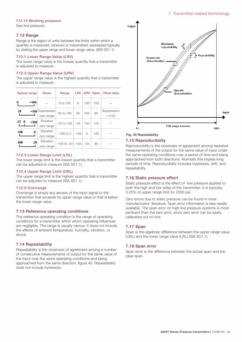
2600T Series Pressure transmitters | TI/266-EN 29
7. Transmitter-related terminology
7.11.14 Working pressureSee line pressure.
7.12 Range Range is the region of units between the limits within which a
quantity is measured, received or transmitted, expressed typically
by stating the upper range and lower range value, (ISA S51.1)
7.12.1 Lower Range Value (LRV)The lower range value is the lowest quantity that a transmitter
is adjusted to measure.
7.12.2 Upper Range Value (URV)The upper range value is the highest quantity that a transmitter
is adjusted to measure.
Typical range Name Range LRV URV Span Other data
— 0 to 100 0 100 100 —
Suppressed
zero range20 to 100 20 100 80
Suppression
= 0.25
Elevated
zero range-25 to 100 -25 100 125 —
Elevated
zero range-100 to 0 -100 0 100 —
Elevated
zero range-100 to -20 -100 -25 80 —
7.12.3 Lower Range Limit (LRL)The lower range limit is the lowest quantity that a transmitter
can be adjusted to measure (ISA S51.1).
7.12.4 Upper Range Limit (URL)The upper range limit is the highest quantity that a transmitter
can be adjusted to measure (ISA S51.1).
7.12.5 OverrangeOverrange is simply any excess of the input signal to the
transmitter that exceeds its upper range value or that is below
the lower range value.
7.13 Reference operating conditionsThe reference operating condition is the range of operating
conditions for a transmitter within which operating infl uences
are negligible. The range is usually narrow. It does not include
the effects of ambient temperature, humidity, vibration, or
shock.
7.14 RepeatabilityRepeatability is the closeness of agreement among a number
of consecutive measurements of output for the same value of
the input over the same operating conditions and being
approached from the same direction, fi gure 40. Repeatability
does not include hysteresis.
Fig. 40 Repeatability
7.15 Reproducibility Reproducibility is the closeness of agreement among repeated
measurements of the output for the same value of input under
the same operating conditions over a period of time and being
approached from both directions. Normally this implies long
periods of time. Reproducibility includes hysteresis, drift, and
repeatability.
7.16 Static pressure effectStatic pressure effect is the effect of -line pressure applied to
both the high and low sides of the transmitter. It is typically:
0.25% of upper range limit for 2000 psi
Zero errors due to static pressure can be found in most
manufacturers’ literature. Span error information is less readily
available. The span error on high line pressure systems is more
pertinent than the zero error, since zero error can be easily
calibrated out on-line.
7.17 Span Span is the algebraic difference between the upper range value
(URL) and the lower range value (LRL) (ISA S51.1).
7.18 Span error Span error is the difference between the actual span and the
ideal span.
30 TI/266-EN | 2600T Series Pressure transmitters
7. Transmitter-related terminology
7.19 Temperature effect The temperature effect, unless otherwise stated, is assumed to
include both the zero error and the total effect. It can be
expressed as:
— ± 1-0% of maximum span per 100 °F
— ± 1-0% of maximum span per 100 °F between 50 °F and
150 °F
± 1-0% of Maximum Span per 100 °F. This specifi cation implies that the temperature effect is ± 1-0%
of the upper range value for any 100 °F change in temperature
within the operating limits of the transmitter.
± 1.0% of Maximum Span per 100°F between 50°F and 150°F. This specifi cally calls out a specifi c range of temperature over
which the statement applies. This range is generally a subset of
the operating range of the transmitter. The specifi cation does
not apply if you are operating within the operating range of the
transmitter, but outside the specifi cation limits.
Temperature effect is generally defi ned in specifi cations at the
maximum span. As the transmitter is turned down and smaller
spans than maximum are measured, the temperature effect is
magnifi ed. This is true for all transmitters. As a rule of thumb,
the worst-case temperature effect is magnifi ed to the same
extent as the transmitter turn down ratio. The following
example shows how to determine temperature effect for span
settings less than the maximum limit.
On Zero:
Temperature Effect Statement: ± 0.5% /100 °F (50 °C) at
maximum span.
Span Limit: 0-25” w.c. to 0-150” w.c.
Calibrated Range: 0-25” w.c.
Temperature Change: 80° up to 180 °F (26 °C up to 82 °C), a
100 °F (56 °C) change.
Turn Down Ratio: 150/25 = 6:1
Temperature Effect at Calibrated Span: 6 x ± 0.5% =
3%/100 °F
Zero on transmitter may shift by (3% x 150”) = ± 4.5”
Because of the magnifi ed effects of temperature at low span
settings, most users will select a transmitter that works as
close to maximum range conditions as possible. In addition,
users try to eliminate the effects on ambient and process
temperature changes on the transmitter installation. For
example, a transmitter should not be installed outdoors where
it is unprotected from direct sunlight, especially if it is being
used near its minimum span limit.
7.20 Turn Down The Turn Down Ratio of a transmitter is the ratio between its
Upper Range Limit and the minimum recommended span. Some
time it is also called rangeability. It represents the capability of
the transmitter to cover several pressure ranges, without
deteriorating the transmitter performance: accuracy, etc.
7.21 Vibration effectMost specifi cations associated with vibration refer to sinusoidal
vibration, which may or may not be the type of vibration
exhibited in service. The ability of the transmitter to withstand
shock is often as important as the vibration considerations. It is
diffi cult to perform laboratory tests that relate well to the
ruggedness of a unit in a given environment, so that trial
installations tend to be much more reliable.
7.22 Zero errorZero error is the difference between the actual zero and the
ideal zero.

2600T Series Pressure transmitters | TI/266-EN 31
Products and customer support
ABB’s portfolio for valve automation:− Continuous electrical actuators and pneumatic actuators
− Electro-pneumatic, pneumatic, and digital positioners
− I/P signal converters
ABB’s pressure measurement:− Absolute, gauge and differential pressure transmitters
− IEC 61508 SIL2/3 certifi ed pressure transmitters and switches
− Multivariable transmitters
− Interface level/density transmitters
− Pressure measurement remote seals
− Pressure measurement accessories
− Pneumatic pressure transmitters
ABB’s temperature measurement:− Universal temperature sensors
− High-temperature sensors
− Temperature sensors for sanitary applications
− Mineral isolated temperature sensors
− Thermowells
− Temperature transmitters
− IEC 61508 SIL2/3 certified temperature sensors and
transmitters
ABB’s portfolio of recorders and controllers:− Process controllers and indicators
− Videographic recorders
− Paper chart recorders
− Field mountable indicators and controllers
ABB’s portfolio of level measurement:− Magnetic level gauges
− Magnetostrictive and guided wave radar level transmitters
− Laser and scanner level transmitters
− Ultrasonic, capacitance and vibrating fork level transmitters
and switches
− Rotating paddle and thermal dispersion level switches
− IEC 61508 SIL2/3 certifi ed level transmitters
ABB’s portfolio of device management:− Fieldbus and wireless solutions
− Scalable asset & device management
− Asset vision software
− Mobility handhelds
Customer supportWe provide a comprehensive after sales service via a
Worldwide Service Organization.
Contact one of the following offi ces for details on your nearest
Service and Repair Centre.
ABB S.p.A.Via Statale 113,
22016 Lenno (Co) – Italy
Tel: +39 0344 58111
Fax: +39 0344 56278
ABB Automation Product GmbHSchillerstrasse 72
D-32425 Minden – Germany
Tel: +49 551 905534
Fax: +49 551 905555
ABB Inc.125 E. County Line Road
Warminster, PA 18974 – USA
Tel: +1 215 6746000
Fax: +1 215 6747183
ABB Inc.
3450 Harvester Road
Burlington, Ontario L7N 3W5 – Canada
Tel: +1 905 6810565
Fax: +1 905 6812810
ABB Ltd.32 Industrial Area, NIT,
Faridabad - 121 001, Haryana – India
Tel: +91 129 2448300
Fax: +91 129 2440622
ABB Engineering (Shanghai) Ltd.No.5, Lane 369, Chuangye Rd., Pudong District,
Shanghai 201319 - P.R. China
Tel: +86 21 6105 6666
Fax +86 21 6105 6677

TI/
26
6-E
N 0
1.2
01
2ABB Ltd.Process AutomationHoward Road, St. Neots
Cambridgeshire, PE19 8EU
UK
Tel: +44 (0)1480 475321
Fax: +44 (0)1480 217948
ABB Inc.Process Automation125 E. County Line Road
Warminster, PA 18974
USA
Tel: +1 215 674 6000
Fax: +1 215 674 7183
ABB Automation Product GmbHSchillerstrasse 72
D-32425 Minden
Germany
Tel: +49 551 905534
Fax: +49 551 905555
ABB S.p.A.Process AutomationVia Statale 113
22016 Lenno (CO),
Italy
Tel: +39 0344 58111
Fax: +39 0344 56278
www.abb.com/measurement
Contact us
Note
We reserve the right to make technical changes or
modify the contents of this document without prior
notice. With regard to purchase orders, the agreed
particulars shall prevail. ABB does not accept any
responsibility whatsoever for potential errors or
possible lack of information in this document.
We reserve all rights in this document and in the
subject matter and illustrations contained therein.
Any reproduction, disclosure to third parties or
utilization of its contents - in whole or in parts – is
forbidden without prior written consent of ABB.
Copyright© 2012 ABB
All rights reserved
3KXP000001R2901
Recommended