1
Water Demand and Water Distribution System Design
Robert PittUniversity of AlabamaUniversity of Alabama
Distribution of per capita water demand
(Chin 2000 Table 3.5)
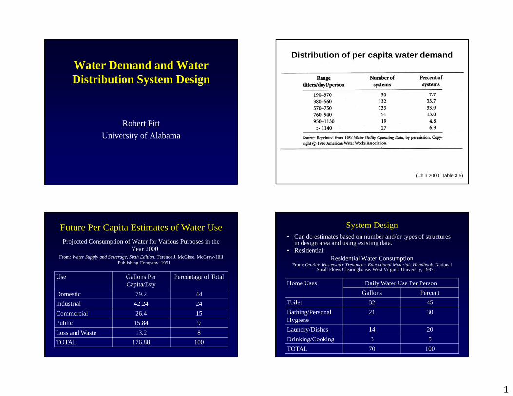
Future Per Capita Estimates of Water UseProjected Consumption of Water for Various Purposes in the
Year 2000From: Water Supply and Sewerage, Sixth Edition. Terence J. McGhee. McGraw-Hill
Publishing Company. 1991.
Use Gallons Per Capita/Day
Percentage of Total
Domestic 79.2 44Industrial 42.24 24Commercial 26.4 15Public 15.84 9Loss and Waste 13.2 8TOTAL 176.88 100
System Design• Can do estimates based on number and/or types of structures
in design area and using existing data.• Residential:
Residential Water Consumptiones de t a Wate Co su pt oFrom: On-Site Wastewater Treatment: Educational Materials Handbook. National
Small Flows Clearinghouse. West Virginia University, 1987.
Home Uses Daily Water Use Per PersonGallons Percent
Toilet 32 45Bathing/Personal Hygiene
21 30
Laundry/Dishes 14 20Drinking/Cooking 3 5TOTAL 70 100
2
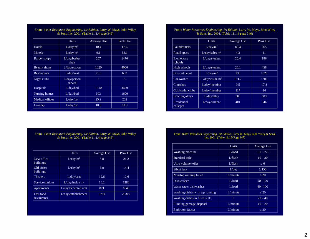
From: Water Resources Engineering, 1st Edition. Larry W. Mays, John Wiley & Sons, Inc. 2001. (Table 11.1.4 page 346)
Units Average Use Peak Use
Hotels L/day/m2 10.4 17.6
Motels L/day/m2 9 1 63 1Motels L/day/m 9.1 63.1
Barber shops L/day/barber chair
207 1470
Beauty shops L/day/station 1020 4050
Restaurants L/day/seat 91.6 632
Night clubs L/day/person d
5 5served
Hospitals L/day/bed 1310 3450
Nursing homes L/day/bed 503 1600
Medical offices L/day/m2 25.2 202
Laundry L/day/m2 10.3 63.9
From: Water Resources Engineering, 1st Edition. Larry W. Mays, John Wiley & Sons, Inc. 2001. (Table 11.1.4 page 346)
Units Average Use Peak Use
Laundromats L/day/m2 88.4 265
Retail space L/day/sales m2 4 3 11Retail space L/day/sales m 4.3 11
Elementary schools
L/day/student 20.4 186
High schools L/day/student 25.1 458
Bus-rail depot L/day/m2 136 1020
Car washes L/day/inside m2 194.7 1280
Churches L/day/member 0.5 17.8
Golf-swim clubs L/day/member 117 84
Bowling alleys L/day/alley 503 503
Residential colleges
L/day/student 401 946
From: Water Resources Engineering, 1st Edition. Larry W. Mays, John Wiley & Sons, Inc. 2001. (Table 11.1.4 page 346)
Units Average Use Peak Use
New office buildings
L/day/m2 3.8 21.2
Old office buildings
L/day/m2 5.8 14.4
Theaters L/day/seat 12.6 12.6
Service stations L/day/inside m2 10.2 1280
Apartments L/day/occupied unit 821 1640
Fast food restaurants
L/day/establishment 6780 20300
From: Water Resources Engineering, 1st Edition. Larry W. Mays, John Wiley & Sons, Inc. 2001. (Table 11.1.5 Page 347)
Units Average Use
Washing machine L/load 130 – 270
St d d t il t L/fl h 10 30Standard toilet L/flush 10 – 30
Ultra volume toilet L/flush 6
Silent leak L/day 150
Nonstop running toilet L/minute 20
Dishwasher L/load 50 –120
Water saver dishwasher L/load 40 100Water-saver dishwasher L/load 40 –100
Washing dishes with tap running L/minute 20
Washing dishes in filled sink L 20 – 40
Running garbage disposal L/minute 10 – 20
Bathroom faucet L/minute 20
3
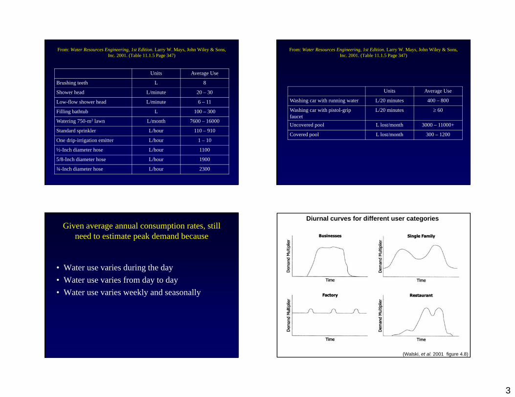
From: Water Resources Engineering, 1st Edition. Larry W. Mays, John Wiley & Sons, Inc. 2001. (Table 11.1.5 Page 347)
Units Average Use
Brushing teeth L 8
Shower head L/minute 20 – 30
Low-flow shower head L/minute 6 – 11
Filling bathtub L 100 – 300
Watering 750-m2 lawn L/month 7600 – 16000
Standard sprinkler L/hour 110 – 910
One drip-irrigation emitter L/hour 1 – 10
½-Inch diameter hose L/hour 1100
5/8-Inch diameter hose L/hour 1900
¾-Inch diameter hose L/hour 2300
From: Water Resources Engineering, 1st Edition. Larry W. Mays, John Wiley & Sons, Inc. 2001. (Table 11.1.5 Page 347)
Units Average Use
Washing car with running water L/20 minutes 400 – 800
Washing car with pistol-grip faucet
L/20 minutes 60
Uncovered pool L lost/month 3000 – 11000+
Covered pool L lost/month 300 – 1200p
Given average annual consumption rates, still need to estimate peak demand because
• Water use varies during the day• Water use varies from day to day• Water use varies weekly and seasonally
Diurnal curves for different user categories
(Walski, et al. 2001 figure 4.8)
4
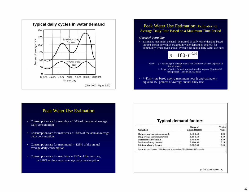
Typical daily cycles in water demand
(Chin 2000 Figure 3.23)
Peak Water Use Estimation: Estimation of Average Daily Rate Based on a Maximum Time Period
Goodrich Formula:• Estimates maximum demand (expressed as daily water demand based ( p y
on time period for which maximum water demand is desired) for community when given annual average per capita daily water use rate:
where p = percentage of average annual rate (volume/day) used in period of time of interest
10.0180 tp
time of interestt = length of period for which peak demand is required (days) (valid
time periods – 2 hours to 360 days)
• **Daily rate based upon a maximum hour is approximately equal to 150 percent of average annual daily rate.
Peak Water Use Estimation
• Consumption rate for max day = 180% of the annual average daily consumptiony p
• Consumption rate for max week = 148% of the annual average daily consumption
• Consumption rate for max month = 128% of the annual average daily consumption
• Consumption rate for max hour = 150% of the max day, or 270% of the annual average daily consumption
Typical demand factors
(Chin 2000 Table 3.6)
5
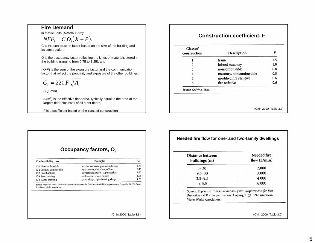
iiii PXOCNFF In metric units (AWWA 1992):
C is the construction factor based on the size of the building and its construction,
Fire Demand
O is the occupancy factor reflecting the kinds of materials stored in the building (ranging from 0.75 to 1.25), and
(X+P) is the sum of the exposure factor and the communication factor that reflect the proximity and exposure of the other buildings.
AFC 220 ii AFC 220C (L/min),
A (m2) is the effective floor area, typically equal to the area of the largest floor plus 50% of all other floors,
F is a coefficient based on the class of construction
Construction coefficient, F
(Chin 2000 Table 3.7)
Occupancy factors, Oi
(Chin 2000 Table 3.8)
Needed fire flow for one- and two-family dwellings
(Chin 2000 Table 3.9)
6
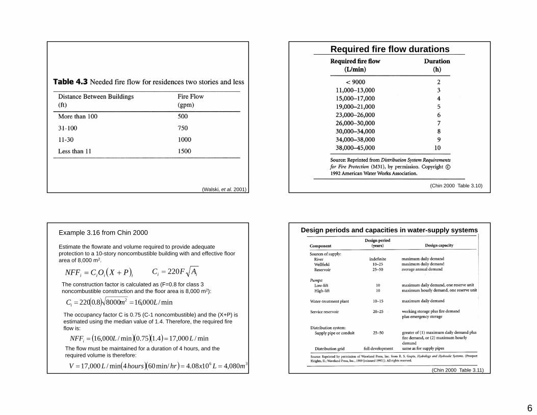
(Walski, et al. 2001)
Required fire flow durations
(Chin 2000 Table 3.10)
Example 3.16 from Chin 2000
Estimate the flowrate and volume required to provide adequate protection to a 10-story noncombustible building with and effective floor area of 8,000 m2.
PXOCNFF AFC 220 iiii PXOCNFF ii AFC 220
min/000,1680008.0220 2 LmCi
The construction factor is calculated as (F=0.8 for class 3 noncombustible construction and the floor area is 8,000 m2):
The occupancy factor C is 0.75 (C-1 noncombustible) and the (X+P) is estimated using the median value of 1.4. Therefore, the required fire
min/000,174.175.0min/000,16 LLNFFi
36 080,41008.4min/604min/000,17 mLxhrhoursLV
estimated using the median value of 1.4. Therefore, the required fire flow is:
The flow must be maintained for a duration of 4 hours, and the required volume is therefore:
Design periods and capacities in water-supply systems
(Chin 2000 Table 3.11)

7
Methods of Water Distribution
• Pumping with StorageM t– Most common
– Water supplied at approximately uniform rate– Flow in excess of consumption stored in elevated tanks– Tank water provides flow and pressure when use is high
• Fire-fighting• High-use hours• Flow during power failure
– Storage volume throughout system and for individual service areas should be approximately 15 – 30% of maximum daily rate.
Water Distribution System Components
• Pumping Stations• Distribution Storage• Distribution System Piping
Other water system components include water source and water treatment
Looped and branched networks after network failure
(Walski, et al. 2001 figure 1.2)
The Pipe System
• Primary Mains (Arterial Mains)– Form the basic structure of the system and carry
flow from the pumping station to elevated storage tanks and from elevated storage tanks to the various districts of the city
• Laid out in interlocking loopsM i t th 1 k (3000 ft) t• Mains not more than 1 km (3000 ft) apart
• Valved at intervals of not more than 1.5 km (1 mile)• Smaller lines connecting to them are valved

8
The Pipe System, Cont.
• Secondary Lines– Form smaller loops within the primary main
system– Run from one primary line to another– Spacings of 2 to 4 blocks– Provide large amounts of water for fire fighting g g g
with out excessive pressure loss
The Pipe System, Cont.
• Small distribution lines– Form a grid over the entire service area– Supply water to every user and fire hydrants– Connected to primary, secondary, or other small
mains at both ends– Valved so the system can be shut down for repairsy p– Size may be dictated by fire flow except in
residential areas with very large lots
Pipe sizes in Municipal Distribution Systems
• Small distribution lines providing only domestic flow may be as small as 4 inches, but:
< 1300 ft in length if dead ended or– < 1300 ft in length if dead ended, or – < 2000 ft if connected to system at both ends.
• Otherwise, small distribution mains > 6 in • High value districts – minimum size 8 in• Major streets – minimum size 12 in
• Fire-fighting requirements> 150 mm (6 in.)
• National Board of Fire Underwriters> 200 mm (8 in.)
Velocity in Municipal Distribution Systems
(McGhee, Water Supply and Sewerage, 6th Edition)• Normal use < 1m/s, (3 ft/s)• Upper limit = 2 m/s (6 ft/s) (may occur in
vicinity of large fires)
(Viessman and Hammer, Water Supply and Pollution Control, 6th Edition)
1< V < 1.7 m/s (3 < V < 5 ft/s)

9
Pressure in Municipal Distribution Systems(American Water Works Association)
AWWA recommends normal static pressure of 400-500kPa, 60-75lb/in2
- supplies ordinary uses in building up to 10 stories- will supply sprinkler system in buildings up to 5
stories- will provide useful fire flow without pumper trucks- will provide a relatively large margin of safety to
offset sudden high demand or closure of partof the system.
Pressure in Municipal Distribution Systems(McGee)
• Pressure in the range of 150 – 400kPa (20 to 40 lb/in2) are adequate for normal use and may be used for fire supply in small towns where building heights do not exceed 4 stories.
Minimum acceptable pressures in distribution systems
(Chin 2000 Table 3.12)
Typical elevated storage tank
(Chin 2000 Figure 3.24)
10
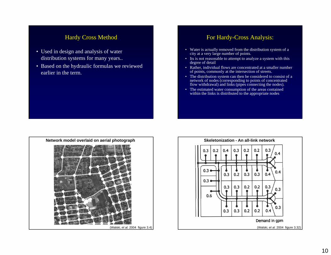
Hardy Cross Method
• Used in design and analysis of water di t ib ti t fdistribution systems for many years..
• Based on the hydraulic formulas we reviewed earlier in the term.
For Hardy-Cross Analysis:
• Water is actually removed from the distribution system of a city at a very large number of points.
• Its is not reasonable to attempt to analyze a system with this degree of detail
• Rather, individual flows are concentrated at a smaller number of points, commonly at the intersection of streets.
• The distribution system can then be considered to consist of a network of nodes (corresponding to points of concentrated flow withdrawal) and links (pipes connecting the nodes).
• The estimated water consumption of the areas contained within the links is distributed to the appropriate nodes
Network model overlaid on aerial photograph
(Walski, et al. 2004 figure 3.4)
Skeletonization - An all-link network
(Walski, et al. 2004 figure 3.32)
11
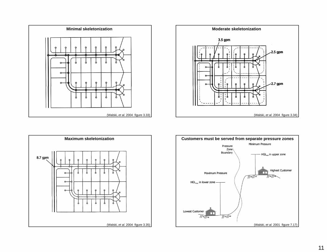
Minimal skeletonization
(Walski, et al. 2004 figure 3.33)
Moderate skeletonization
(Walski, et al. 2004 figure 3.34)
Maximum skeletonization
(Walski, et al. 2004 figure 3.35)
Customers must be served from separate pressure zones
(Walski, et al. 2001 figure 7.17)
12
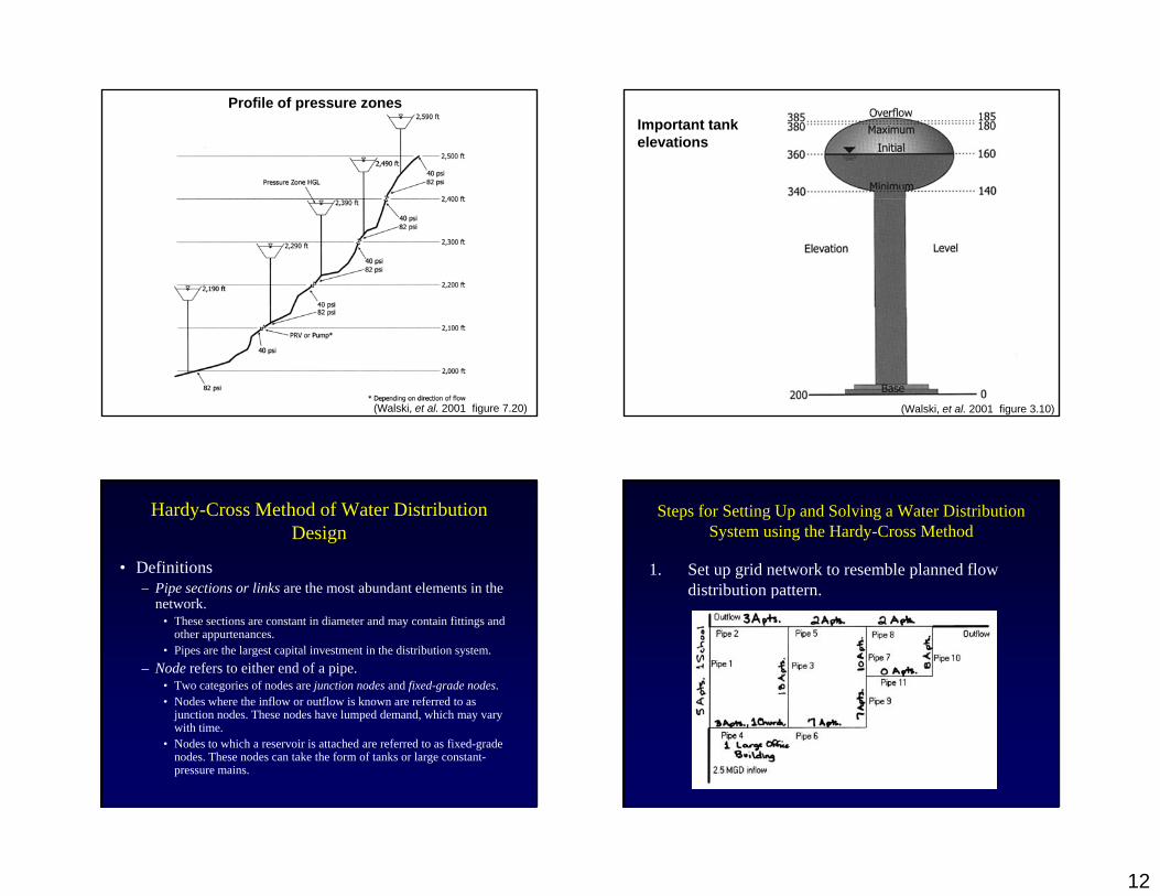
Profile of pressure zones
(Walski, et al. 2001 figure 7.20)
Important tank elevations
(Walski, et al. 2001 figure 3.10)
Hardy-Cross Method of Water Distribution Design
• Definitions– Pipe sections or links are the most abundant elements in the– Pipe sections or links are the most abundant elements in the
network. • These sections are constant in diameter and may contain fittings and
other appurtenances. • Pipes are the largest capital investment in the distribution system.
– Node refers to either end of a pipe. • Two categories of nodes are junction nodes and fixed-grade nodes.
N d h h i fl fl i k f d• Nodes where the inflow or outflow is known are referred to as junction nodes. These nodes have lumped demand, which may vary with time.
• Nodes to which a reservoir is attached are referred to as fixed-grade nodes. These nodes can take the form of tanks or large constant-pressure mains.
Steps for Setting Up and Solving a Water Distribution System using the Hardy-Cross Method
1. Set up grid network to resemble planned flow distribution patterndistribution pattern.
13
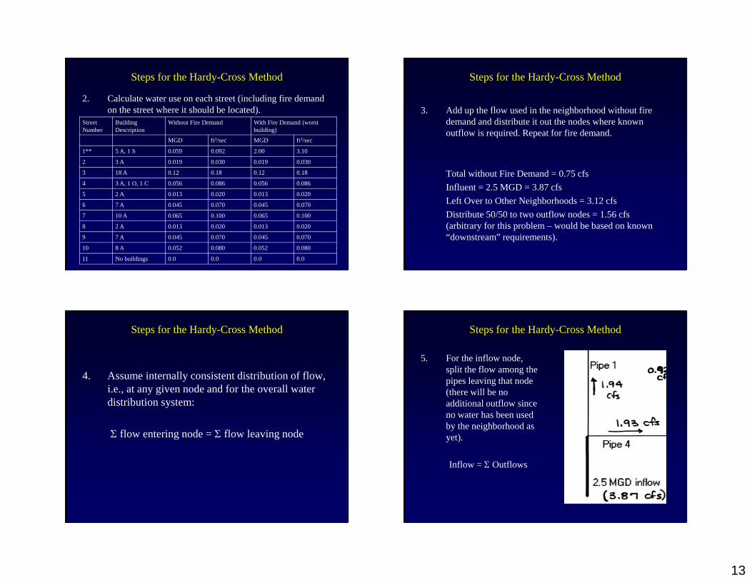
Steps for the Hardy-Cross Method
2. Calculate water use on each street (including fire demand on the street where it should be located).
Street N b
Building D i ti
Without Fire Demand With Fire Demand (worst b ildi )Number Description building)
MGD ft3/sec MGD ft3/sec
1** 5 A, 1 S 0.059 0.092 2.00 3.10
2 3 A 0.019 0.030 0.019 0.030
3 18 A 0.12 0.18 0.12 0.18
4 3 A, 1 O, 1 C 0.056 0.086 0.056 0.086
5 2 A 0.013 0.020 0.013 0.020
6 7 A 0.045 0.070 0.045 0.070
7 10 A 0.065 0.100 0.065 0.100
8 2 A 0.013 0.020 0.013 0.020
9 7 A 0.045 0.070 0.045 0.070
10 8 A 0.052 0.080 0.052 0.080
11 No buildings 0.0 0.0 0.0 0.0
Steps for the Hardy-Cross Method
3. Add up the flow used in the neighborhood without fire demand and distribute it out the nodes where known outflow is required. Repeat for fire demand.
Total without Fire Demand = 0.75 cfsInfluent = 2.5 MGD = 3.87 cfsL ft O t Oth N i hb h d 3 12 fLeft Over to Other Neighborhoods = 3.12 cfsDistribute 50/50 to two outflow nodes = 1.56 cfs (arbitrary for this problem – would be based on known “downstream” requirements).
Steps for the Hardy-Cross Method
4. Assume internally consistent distribution of flow, yi.e., at any given node and for the overall water distribution system:
flow entering node = flow leaving node
Steps for the Hardy-Cross Method
5. For the inflow node, split the flow among the pipes leaving that nodepipes leaving that node (there will be no additional outflow since no water has been used by the neighborhood as yet).
Inflow = Outflows
14
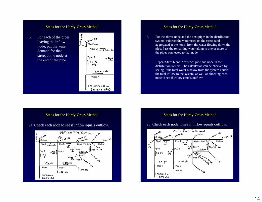
Steps for the Hardy-Cross Method
6. For each of the pipes leaving the inflow node, put the water demand for that street at the node at the end of the pipe.
Steps for the Hardy-Cross Method
7. For the above node and the next pipes in the distribution system, subtract the water used on the street (and aggregated at the node) from the water flowing down theaggregated at the node) from the water flowing down the pipe. Pass the remaining water along to one or more of the pipes connected to that node.
8. Repeat Steps 6 and 7 for each pipe and node in the distribution system. The calculation can be checked by seeing if the total ater o tflo from the s stem eq alsseeing if the total water outflow from the system equals the total inflow to the system, as well as checking each node to see if inflow equals outflow.
Steps for the Hardy-Cross Method
9a. Check each node to see if inflow equals outflow.
Steps for the Hardy-Cross Method
9b. Check each node to see if inflow equals outflow.

15
Steps for the Hardy-Cross Method10. Select initial pipe sizes (assume a velocity of 3 ft/sec for normal flow with no fire
demand). With a known/assumed flow and an assumed velocity, use the continuity equation (Q = VA) to calculate the cross-sectional area of flow. (when conducting computer design, set diameters to minimum allowable diameters for each type of neighborhood according to local regulations)
Pipe Flo (ft3/sec) Velocit Area (ft2) Diameter Diameter Act al DPipe Number
Flow (ft3/sec) Velocity (ft/sec)
Area (ft2) Diameter (ft)
Diameter (in)
Actual D (in)
1 1.94 3.0 0.65 0.91 10.9 12
2 0.288 3.0 0.10 0.35 4.2 6
3 0.922 3.0 0.31 0.63 7.5 8
4 1.930 3.0 0.64 0.91 10.9 12
5 1.000 3.0 0.33 0.65 7.8 8
6 0 922 3 0 0 31 0 63 7 5 86 0.922 3.0 0.31 0.63 7.5 8
7 0.220 3.0 0.07 0.31 3.7 4
8 1.100 3.0 0.37 0.68 8.2 10
9 0.852 3.0 0.28 0.60 7.2 8
10 0.562 3.0 0.19 0.49 5.9 6
11 0.562 3.0 0.19 0.49 5.9 6
Steps for the Hardy-Cross Method
11. Determine the convention for flow. Generally, clockwise flows are positive and counter-clockwise flows are negative.
Steps for the Hardy-Cross Method
12. Paying attention to sign (+/-), compute the head loss in each element/pipe of the system (such as by using Darcy-Weisbach or Hazen-Williams).
CDQLh
WilliamsHazen
L432.0
85.1
63.2
gV
DLfh
WeisbachDarcy
L 2
2
Steps for the Hardy-Cross Method
13. Compute the sum of the head losses around each loop (carrying the appropriate sign throughout the p ( y g pp p g gcalculation).
14. Compute the quantity, head loss/flow (hL/Q), for each element/pipe (note that the signs cancel out, leaving a positive number).leaving a positive number).
15. Compute the sum of the (hL/Q)s for each loop.
16
Steps for the Hardy-Cross Method
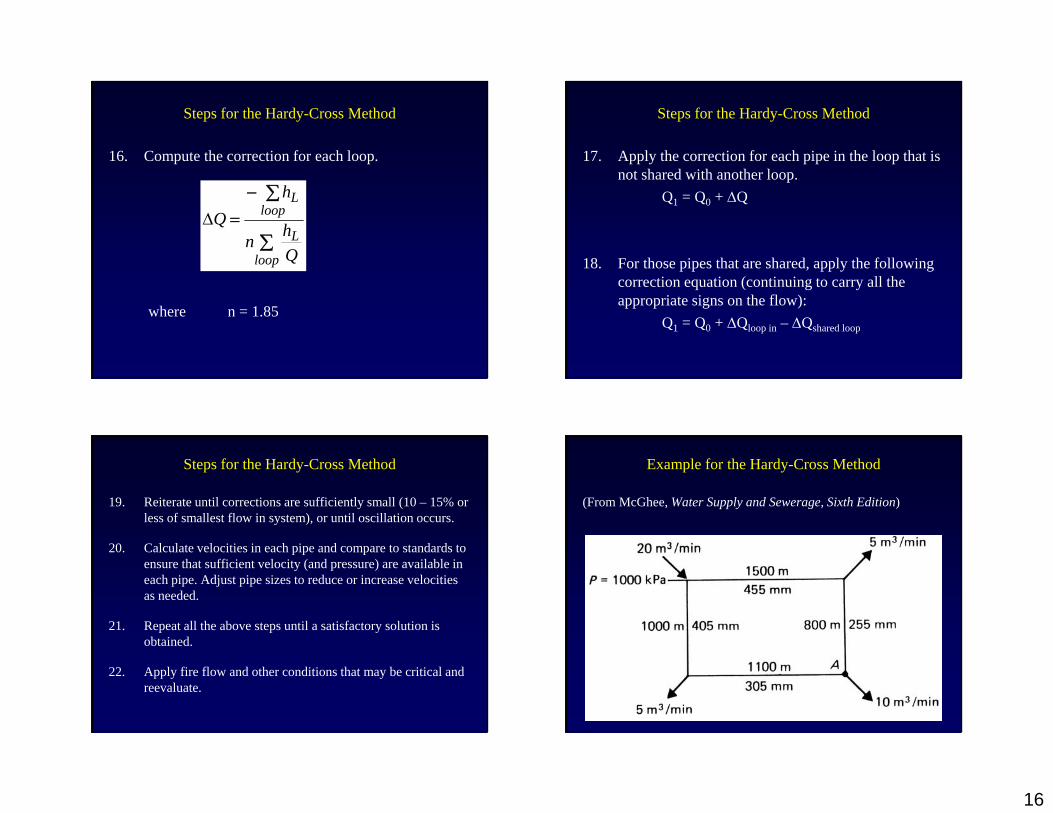
16. Compute the correction for each loop.
loop
L
loopL
Qhn
hQ
where n = 1.85
Steps for the Hardy-Cross Method
17. Apply the correction for each pipe in the loop that is not shared with another loop.p
Q1 = Q0 + Q
18. For those pipes that are shared, apply the following ti ti ( ti i t ll thcorrection equation (continuing to carry all the
appropriate signs on the flow):Q1 = Q0 + Qloop in – Qshared loop
Steps for the Hardy-Cross Method
19. Reiterate until corrections are sufficiently small (10 – 15% or less of smallest flow in system), or until oscillation occurs.
20. Calculate velocities in each pipe and compare to standards to ensure that sufficient velocity (and pressure) are available in each pipe. Adjust pipe sizes to reduce or increase velocities as needed.
21. Repeat all the above steps until a satisfactory solution is obtained.
22. Apply fire flow and other conditions that may be critical and reevaluate.
Example for the Hardy-Cross Method
(From McGhee, Water Supply and Sewerage, Sixth Edition)
17
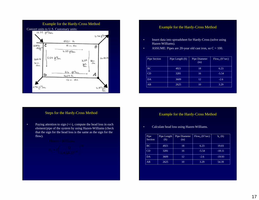
Example for the Hardy-Cross MethodConvert units to U.S. Customary units: Example for the Hardy-Cross Method
• Insert data into spreadsheet for Hardy-Cross (solve using Hazen-Williams).Hazen Williams).
• ASSUME: Pipes are 20-year old cast iron, so C = 100.
Pipe Section Pipe Length (ft) Pipe Diameter (in)
Flow0 (ft3/sec)
BC 4921 18 6 23BC 4921 18 6.23
CD 3281 16 -5.54
DA 3609 12 -2.6
AB 2625 10 3.29
Steps for the Hardy-Cross Method
• Paying attention to sign (+/-), compute the head loss in each element/pipe of the system by using Hazen-Williams (check th t th i f th h d l i th th i f ththat the sign for the head loss is the same as the sign for the flow).
85.1
63.2432.0
CDQLh
WilliamsHazen
L
Example for the Hardy-Cross Method
• Calculate head loss using Hazen-Williams.
Pipe Section
Pipe Length (ft)
Pipe Diameter (in)
Flow0 (ft3/sec) hL (ft)
BC 4921 18 6.23 19.03
CD 3281 16 -5.54 -18.11
DA 3609 12 2 6 19 93DA 3609 12 -2.6 -19.93
AB 2625 10 3.29 54.39
18
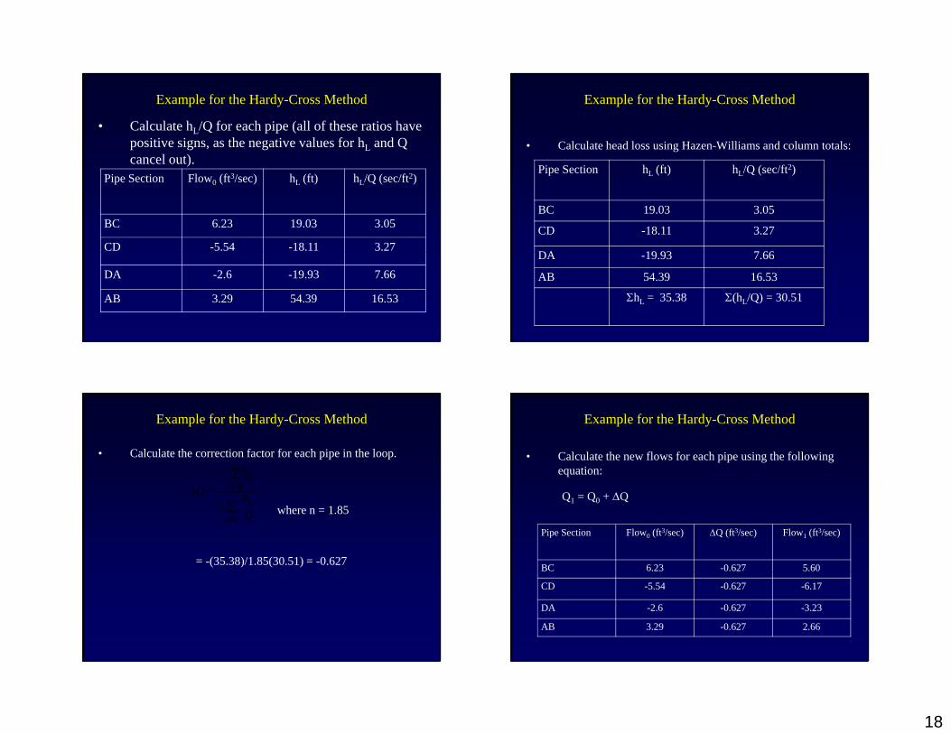
Example for the Hardy-Cross Method
• Calculate hL/Q for each pipe (all of these ratios have positive signs, as the negative values for hL and Q cancel out).cancel out).
Pipe Section Flow0 (ft3/sec) hL (ft) hL/Q (sec/ft2)
BC 6.23 19.03 3.05
CD -5.54 -18.11 3.27
DA -2.6 -19.93 7.66
AB 3.29 54.39 16.53
Example for the Hardy-Cross Method
• Calculate head loss using Hazen-Williams and column totals:
Pipe Section hL (ft) hL/Q (sec/ft2)
BC 19.03 3.05
CD -18.11 3.27
DA 19 93 7 66DA -19.93 7.66
AB 54.39 16.53
hL = 35.38 (hL/Q) = 30.51
Example for the Hardy-Cross Method
• Calculate the correction factor for each pipe in the loop.
l
Lh
where n = 1.85
loop
L
loop
Qhn
Q
= -(35.38)/1.85(30.51) = -0.627
Example for the Hardy-Cross Method
• Calculate the new flows for each pipe using the following equation:
Q1 = Q0 + Q
Pipe Section Flow0 (ft3/sec) Q (ft3/sec) Flow1 (ft3/sec)
BC 6.23 -0.627 5.60
CD -5.54 -0.627 -6.17
DA -2.6 -0.627 -3.23
AB 3.29 -0.627 2.66
19
Example for the Hardy-Cross MethodHARDY CROSS METHOD FOR WATER SUPPLY DISTRIBUTION
Trial IPipe Section Pipe Length
(f t)Pipe Diameter
(in)Flow 0
(f t3/sec)HL (f t)
HL/Q (sec/f t2)
n(HL/Q) (sec/ft2) (HL) (f t) Q (f t3/sec) Flow 1
(f t3/sec)BC 4921 18 6.2 19.03 3.05 -0.627 5.60CD 3281 16 -5.5 -18.11 3.27 -0.627 -6.17DA 3609 12 -2.6 -19.93 7.66 -0.627 -3.23BA 2625 10 3.3 54.39 16.53 -0.627 2.66
Trial 2Pipe Section Pipe Length
(f t)Pipe Diameter
(in)Flow 1
(f t3/sec)HL (f t)
HL/Q (sec/f t2)
n(HL/Q) (sec/ft2) (HL) (f t) Q (f t3/sec) Flow 2
(f t3/sec)BC 4921 18 5.60 15.64 2.79 -0.012 5.59CD 3281 16 -6.17 -22.08 3.58 -0.012 -6.18DA 3609 12 -3.23 -29.71 9.21 -0.012 -3.24
56.46 35.38
54.38 0.64
BA 2625 10 2.66 36.79 13.81 -0.012 2.65
Trial 3Pipe Section Pipe Length
(f t)Pipe Diameter
(in)Flow 2
(f t3/sec)HL (f t)
HL/Q (sec/f t2)
n(HL/Q) (sec/ft2) (HL) (f t) Q (f t3/sec) Flow 3
(f t3/sec)BC 4921 18 5.59 15.58 2.79 0.000 5.59CD 3281 16 -6.18 -22.16 3.59 0.000 -6.18DA 3609 12 -3.24 -29.91 9.24 0.000 -3.24BA 2625 10 2.65 36.49 13.76 0.000 2.65
54.34 0.00
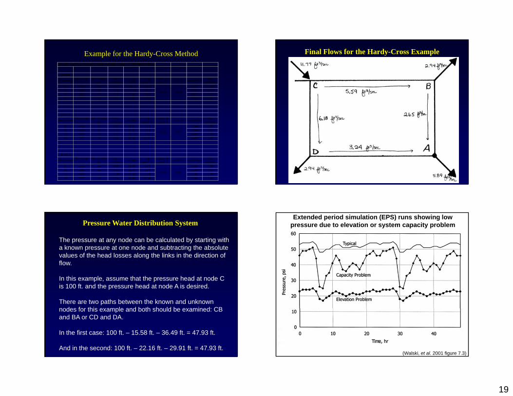
Final Flows for the Hardy-Cross Example
Pressure Water Distribution System
The pressure at any node can be calculated by starting with a known pressure at one node and subtracting the absolute values of the head losses along the links in the direction of flow.
In this example, assume that the pressure head at node C is 100 ft. and the pressure head at node A is desired.
There are two paths between the known and unknown nodes for this example and both should be examined: CBnodes for this example and both should be examined: CB and BA or CD and DA.
In the first case: 100 ft. – 15.58 ft. – 36.49 ft. = 47.93 ft.
And in the second: 100 ft. – 22.16 ft. – 29.91 ft. = 47.93 ft.
Extended period simulation (EPS) runs showing low pressure due to elevation or system capacity problem
(Walski, et al. 2001 figure 7.3)
20
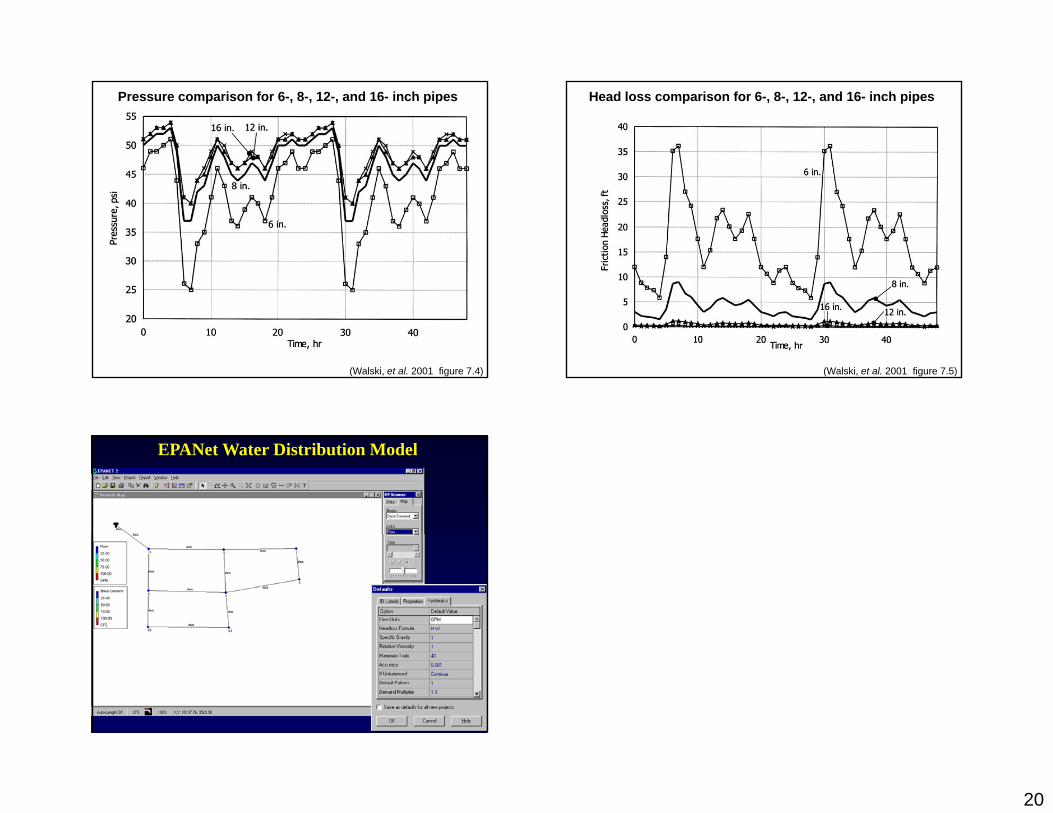
Pressure comparison for 6-, 8-, 12-, and 16- inch pipes
(Walski, et al. 2001 figure 7.4)
Head loss comparison for 6-, 8-, 12-, and 16- inch pipes
(Walski, et al. 2001 figure 7.5)
EPANet Water Distribution Model
Recommended