Vortex-induced Vibration of a 5:1 Rectangular CylinderA comparison of wind tunnel sectional model tests
and computational simulations
Dinh Tung Nguyena, David M. Hargreavesa, John S. Owena
aFaculty of Engineering, University of Nottingham, UK
Abstract
Considered to be representative of a generic bridge deck geometry and characterised bya highly unsteady flow field, the 5:1 rectangular cylinder has been the main case studyin a number of studies including the “Benchmark on the Aerodynamics of a Rectangular5:1 Cylinder” (BARC). There are still a number of limitations in the knowledge of (i) themechanism of the vortex-induced vibration (VIV) and (ii) of the turbulence-induced effectfor this particular geometry. Extended computational and wind tunnel studies were thereforeconducted by the authors to address these issues. This paper primarily describes wind tunneland computational studies using a sectional model in an attempt to bring more insight intoPoint (i). By analysing the distribution and correlation of the surface pressure around anelastically mounted 5:1 rectangular cylinders in smooth and turbulent flow, it revealed thatthe VIV was triggered by the motion-induced leading-edge vortex; a strongly correlatedflow feature close to the trailing edge was then responsible for an increase in the structuralresponse.
Keywords: 5:1 rectangular cylinder, BARC, vortex-induced vibration, turbulent flow, windtunnel, LES simulation
1. Introduction1
The rectangular cylinder has been considered as representative of many structures in2
the built environment including the bridge deck. In contrast to the circular cylinder, the3
rectangular cylinder is characterised by permanent separation points at the leading edge4
causing two unstable shear layers which can interact with the after-body length or with each5
other in the wake, significantly affecting its response (Nakamura et al., 1991). Therefore, the6
aerodynamics of the flow field and related aeroelastic responses of this cylinder are highly7
unsteady and complicated, attracting a number of studies including the BARC study (Bruno8
et al., 2014).9
Email addresses: [email protected] (Dinh Tung Nguyen),[email protected] (David M. Hargreaves), [email protected] (John S.Owen)
Preprint submitted to Journal of Wind Engineering and Industrial Aerodynamics January 15, 2018
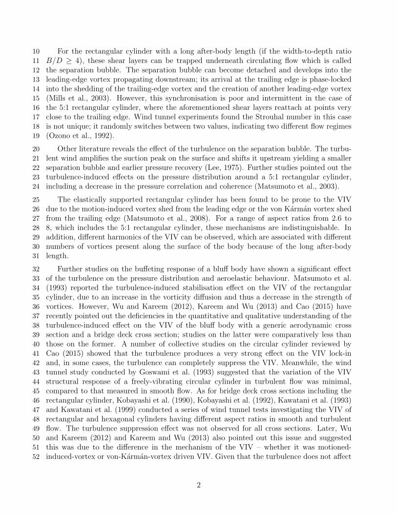
For the rectangular cylinder with a long after-body length (if the width-to-depth ratio10
B/D ≥ 4), these shear layers can be trapped underneath circulating flow which is called11
the separation bubble. The separation bubble can become detached and develops into the12
leading-edge vortex propagating downstream; its arrival at the trailing edge is phase-locked13
into the shedding of the trailing-edge vortex and the creation of another leading-edge vortex14
(Mills et al., 2003). However, this synchronisation is poor and intermittent in the case of15
the 5:1 rectangular cylinder, where the aforementioned shear layers reattach at points very16
close to the trailing edge. Wind tunnel experiments found the Strouhal number in this case17
is not unique; it randomly switches between two values, indicating two different flow regimes18
(Ozono et al., 1992).19
Other literature reveals the effect of the turbulence on the separation bubble. The turbu-20
lent wind amplifies the suction peak on the surface and shifts it upstream yielding a smaller21
separation bubble and earlier pressure recovery (Lee, 1975). Further studies pointed out the22
turbulence-induced effects on the pressure distribution around a 5:1 rectangular cylinder,23
including a decrease in the pressure correlation and coherence (Matsumoto et al., 2003).24
The elastically supported rectangular cylinder has been found to be prone to the VIV25
due to the motion-induced vortex shed from the leading edge or the von Karman vortex shed26
from the trailing edge (Matsumoto et al., 2008). For a range of aspect ratios from 2.6 to27
8, which includes the 5:1 rectangular cylinder, these mechanisms are indistinguishable. In28
addition, different harmonics of the VIV can be observed, which are associated with different29
numbers of vortices present along the surface of the body because of the long after-body30
length.31
Further studies on the buffeting response of a bluff body have shown a significant effect32
of the turbulence on the pressure distribution and aeroelastic behaviour. Matsumoto et al.33
(1993) reported the turbulence-induced stabilisation effect on the VIV of the rectangular34
cylinder, due to an increase in the vorticity diffusion and thus a decrease in the strength of35
vortices. However, Wu and Kareem (2012), Kareem and Wu (2013) and Cao (2015) have36
recently pointed out the deficiencies in the quantitative and qualitative understanding of the37
turbulence-induced effect on the VIV of the bluff body with a generic aerodynamic cross38
section and a bridge deck cross section; studies on the latter were comparatively less than39
those on the former. A number of collective studies on the circular cylinder reviewed by40
Cao (2015) showed that the turbulence produces a very strong effect on the VIV lock-in41
and, in some cases, the turbulence can completely suppress the VIV. Meanwhile, the wind42
tunnel study conducted by Goswami et al. (1993) suggested that the variation of the VIV43
structural response of a freely-vibrating circular cylinder in turbulent flow was minimal,44
compared to that measured in smooth flow. As for bridge deck cross sections including the45
rectangular cylinder, Kobayashi et al. (1990), Kobayashi et al. (1992), Kawatani et al. (1993)46
and Kawatani et al. (1999) conducted a series of wind tunnel tests investigating the VIV of47
rectangular and hexagonal cylinders having different aspect ratios in smooth and turbulent48
flow. The turbulence suppression effect was not observed for all cross sections. Later, Wu49
and Kareem (2012) and Kareem and Wu (2013) also pointed out this issue and suggested50
this was due to the difference in the mechanism of the VIV – whether it was motioned-51
induced-vortex or von-Karman-vortex driven VIV. Given that the turbulence does not affect52
2
the motion-induced vortex, the VIV response can be increased since the turbulence weakens53
the von Karman vortex and its mitigation effects on the motion-induced leading-edge vortex54
(Matsumoto et al., 2008; Wu and Kareem, 2012). Nevertheless, more studies are required to55
clarify these inconsistencies and provide a more comprehensive explanation on the mechanism56
of the turbulence-induced effect on the motion-induced vortex and the VIV.57
Together with traditional wind tunnel tests, the development of Computational Fluid58
Dynamics (CFD) allows researchers to model and investigate the aerodynamics of the flow59
around and the aeroelasticity of the rectangular cylinder. Due to the complexity of the prob-60
lem and the limitation of computational power, simulations were initially restricted to model61
the flow around 2D cylinders using Unsteady Reynolds-Averaged Navier-Stokes (URANS)62
models. Their outcomes agreed well with wind tunnel tests and offered comprehensive ex-63
planation of the vortex shedding phenomenon of the rectangular cylinder (Ohya et al., 1992;64
Tan et al., 1998; Larsen and Walther, 1998). Also, 2D simulations have shown their potential65
in modelling wind-induced responses and extracting aerodynamic and aeroelastic parameters66
such as flutter derivatives (Xiang and Ge, 2002; Owen et al., 2006; Sun et al., 2009; Waterson67
and Baker, 2010). Later, 3D simulations using Large Eddy Simulation (LES) models have68
become more available, focusing on uncovering the characteristics of the separation bubble,69
the effect of the after-body length on the separation and reattachment of the flow and the70
coherence structure of the surface pressure around a static rectangular cylinder (Bruno et al.,71
2010). LES simulations have also been coupled with structural solvers to model the fluid-72
structure interaction (FSI) of a 3D elastically supported rectangular cylinder and bridge deck73
section (Sun et al., 2008; Bai et al., 2013; Zhu and Chen, 2013). These researches highlighted74
the suitability of the LES model to capture the inherent unsteadiness in FSI problems and75
to maintain the flow structure in the wake region in contrast to the over-dissipation of the76
URANS models. Daniels et al. (2014) also applied this method to predict the effect of the free-77
stream turbulence on the aerodynamics of a static and elastically mounted 4:1 rectangular78
cylinder. The use of the LES model is still limited due to its computationally expensive near-79
wall treatment and high mesh density. In addition, Bruno et al. (2011) showed that results80
of 3D LES simulations in the application of the bridge aeroelasticity were very susceptible to81
the level of discretisation in the span-wise direction. Nevertheless, at the current rate of the82
computational development, LES simulation is becoming more favourable to investigate the83
flow field and understand the underlying physical mechanism, such as the aforementioned84
BARC study.85
Extended CFD and wind tunnel studies have been carried out by the authors with the86
aim to bring more insight into the physical mechanism (i) of the VIV as well as (i) of the87
turbulence-induced effect on the VIV of the 5:1 rectangular cylinder. The former is the pri-88
ority focus of this paper. LES simulations and wind tunnel tests are used to investigate the89
flow field around a sectional model in smooth flow. These two approaches were validated by90
comparing selective results of static simulations and wind tunnel static tests with the BARC91
summary statistics. The VIV response of an elastically supported 5:1 rectangular cylinder92
restrained to the heaving or pitching mode only will be measured in the wind tunnel; these93
wind tunnel dynamic tests are complemented by corresponding LES simulations. The analy-94
sis of the surface pressure distribution with the aid of the Proper Orthogonal Decomposition95
(POD) reveals the mechanism of the VIV of this particular geometry and associated flow96
3

features. The outcomes in this paper will be further analysed to offer comprehensive expla-97
nation of the turbulence-induced effect on the VIV, which will be presented in a separate98
paper.99
2. CFD Methodology100
The computations were conducted using the open-source CFD software OpenFOAM101
v2.2.2. The unsteady flow around the rectangular cylinder was modelled using a LES model102
where the Navier-Stokes equations are spatially filtered by the cell size. With the use of103
Boussinesq’s assumption to express the sub-grid scale tensor, the time-dependent filtered104
Navier-Stokes equations are written as105
∂ui∂t
= 0, (1)
∂
∂tρui +
∂
∂xjρuiuj = − p
∂xj+
∂
∂xj
(µ∂ui∂xj
)+
∂
∂xj
[µSGS
(∂ui∂xj
+∂uj∂xi
)], (2)
where i and j are the tensor notation denoting components of the velocity u; ρ and µ are106
the fluid density and dynamic viscosity respectively; p and u are the filtered pressure and107
velocity. µSGS is the sub-grid scale (SGS) viscosity and it is modelled by the use of the108
conventional Smagorinsky SGS model. To avoid the overestimation of the Smagorinsky109
constant and to account for the effects of convection, diffusion, production and destruction110
on the SGS velocity scale, an additional transportation equation is embedded to determine111
the distribution of the kinetic energy of the SGS eddies, kSGS, and the SGS viscosity ,µSGS,112
(Furby et al., 1997)113
∂
∂tρ kSGS +
∂
∂xjρ kSGS uj =
∂
∂xj
(µSGS
∂kSGS
∂xj
)+ 2µSGS Sij Sij − Cε
k3/2SGS
∆, (3)
µSGS = ρCSGS ∆ k1/2SGS, (4)
where the constants are Cε = 1.048 and CSGS = 0.094. ∆ is the characteristic length scale of114
the filter, which is defined as the cubic root of the cell volume. To remove the over-dissipation115
of the kinetic energy in the near-wall region, a filtered width δ according to the van Driest116
approach is introduced as117
δ = min
{∆,
k
C∆
y
(1− exp−
y+
A+
)}, (5)
y+ =
√ρ τw
µy, (6)
4
where k = 0.4187 is the von Karman constant, C∆ = 0.158 and A+ = 26 are the van118
Driest constants. τw is the wall shear stress and y and y+ are the normal distance and119
non-dimensional normal distance to the wall respectively.120
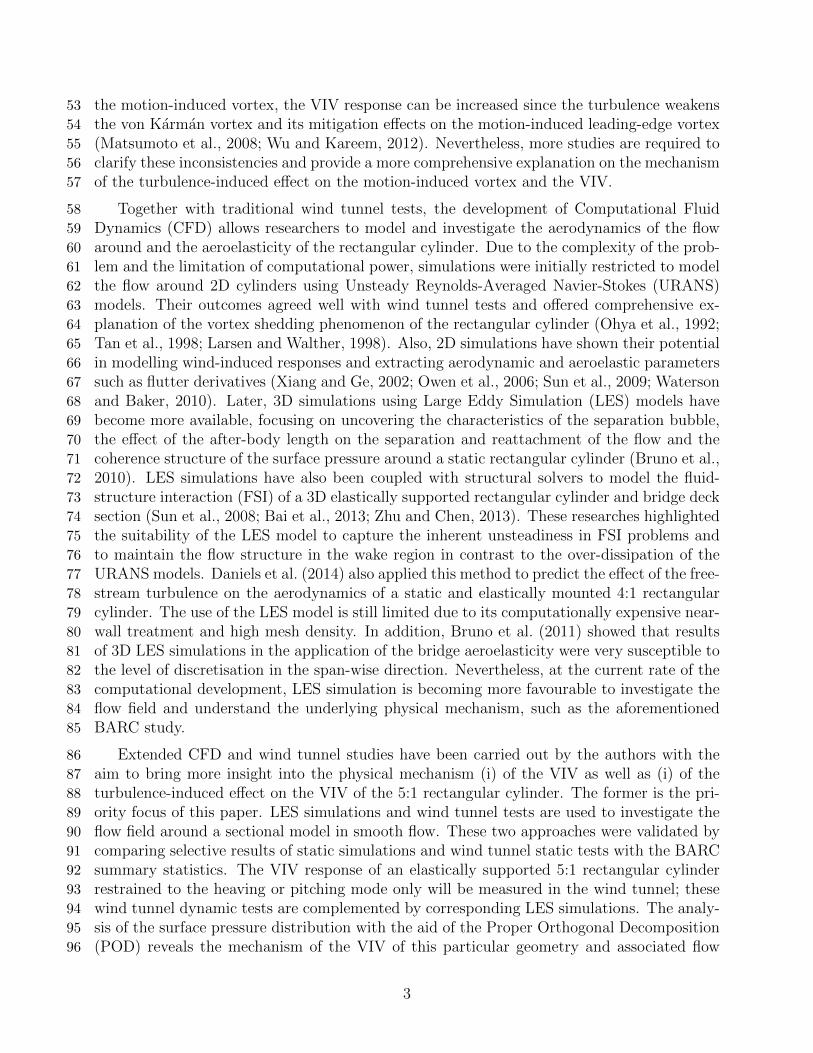
The domain geometry and some key boundary conditions are summarised in Figure 1.121
For the purposes of this computational study, the width of the cylinder. B = 0.5 m, and the122
depth D = 0.1 m. The span-wise length of the cylinder and the width L of the domain was123
3B. The blockage ratio was 4.8%. A zero gradient condition for velocity and a constant value124
of zero gauge pressure were imposed on the outlet. As for the inlet, a non-zero x-component125
wind speed and a zero gradient condition for pressure were specified to simulate smooth flow.126
The OpenFOAM boundary condition movingWallVelocity was applied on the surface of127
the model to accurately model a zero normal-to-wall velocity component at a moving wall.128
The symmetryPlane boundary condition was used for the two z patches while the cyclic129
boundary condition was selected for the two y patches.130
The meshing operation to the domain geometry was conducted using ANSYS-Meshing131
within Workbench and OpenFOAM utilities, fluentMeshToFoam and extrudeMesh. As a132
result, the computational domain was discretised using a 3D hybrid hexahedral grid, where133
the grid was hybrid in the x-z plane (Figure 2a) and structured in the y direction. An134
inflation layer which was a six-cell-thick structured grid was imposed around the model where135
the thickness of cells next to the model was ∆z/B = 2 × 10⁻³ and grew by a ratio of 1.2136
(Figure 2b). The discretisation in the along-wind direction was constant ∆x/B = 2 ∆z/B.137
The unstructured hexahedral grid was used for the remaining part of the x-z plane. The 3D138
grid was constructed by projecting the 2D grid along the y direction; 30 layers was used with139
the span-wise discretisation ∆y/B = 0.1, resulting in a total of 2.1 million cells (Figure 3).140
Figure 1: Domain geometry and boundary conditions of selected patches.
5

(a) (b)
Figure 2: The computational grid in the x-z plane (a) for the entire domain and (b) around the leading edge.
Figure 3: The computational grid used in the 3D heaving simulation.
The pressure-velocity coupling was achieved by means of the PIMPLE algorithm, which141
is a merged PISO-SIMPLE solver. During one time-step, two PISO loops were performed,142
leading to better coupling between pressure and velocity and allowing bigger time-steps and,143
hence, Courant number. The governing equation was spatially discretised using second-144
order schemes. The convection terms were discretised by the use of the limited linear145
scheme while the second-order central differencing scheme was applied to the diffusion terms.146
Non-orthogonal correction factors were enabled to take into account the skewness and non-147
orthogonality of the unstructured grid. As for the temporal discretisation, the implicit148
second-order backward difference scheme was selected. The non-dimensional time-step ∆t? =149
∆t U/B (∆t is the time-step and U is the upstream mean wind speed) was 2× 10−3.150
6

2.1. Static Simulations151
The OpenFOAM solver pimpleFoam was used to simulate the flow around the 3D static152
sectional model at 3 different wind speeds, 1, 2 and 4 m s−1. At each wind speed, the static153
force and moment coefficients were measured and the surface pressure was extracted at se-154
lected points to evaluate the pressure distribution and span-wise correlation. Each simulation155
was extended over 80 non-dimensional time t? = t U/B to obtain converged statistics and156
data in further 120 non-dimensional time was used to perform analysis. Static simulations157
were conducted in parallel on the High Performance Computer (HPC) at the University of158
Nottingham. One simulation was computed in parallel using 32 processors and 8 GB of159
memory; it would take from 1 to 1.5 months to produce reliable data for analysis.160
2.2. Dynamic Simulations161
The coupling procedure between the OpenFOAM solver pimpleDyMFoam and the mass-162
damp-spring equation was utilised to perform the dynamic simulation. The model was re-163
strained to respond in the heaving mode only with the natural frequency of fn,h = 1.2 Hz.164
The model has a mass per unit length of m = 4.7 kg m−1; the damping ratio was ζh = 1%165
yielding the Scruton number Scr = (π m ζh)/(ρB D) of 8.97. The wind speed was increased166
from 0.1 m s−1 to 2.5 m s−1 in increments of 0.1 m s−1 during the lock-in interval.167
A new dynamic mesh class Foam::dynamicHeavingFreeUDFFvMesh was written and im-168
plemented in OpenFOAM to model the heaving motion of the model; this dynamic class169
is also capable to model the pitching response. It contains a structural solver where the170
mass-damping-spring equation was discretised and solved using the the first-order backward171
Euler method172
zn+1 =Fn
m L− 2ωn,h ζh zn + ω2
n,h zn, (7)
zn+1 = zn + ∆t zn+1, (8)
zn+1 = zn + ∆t zn+1, (9)
where zi, zi, zi and Fi are the displacement, velocity and acceleration of and the force acting173
on the model at the time step i; ∆t is the time-step size. The model has the angular natural174
frequency ωn,h and the damping ratio ζh. Here, the backward Euler method was selected175
since it can better model the implicit nature of the FSI problem.176
A dynamic mesh algorithm was implemented based on the linear-spring-analogy algorithm177
proposed by Batina (1990). Since the maximum displacement during the lock-in is relatively178
small (about 10% of the depth of the cross section) and the computational domain was simple,179
this dynamic mesh algorithm is a plausible solution, still maintaining good cell qualities. The180
computational domain was divided into 9 blocks (Figure 4). Blocks 8 and 9 are rigid where181
all grid nodes are fixed relative to the model. The other blocks are grouped into a buffer182
zone where cells are allowed to deform to facilitate the displacement of the model. The183
conventional serial staggered algorithm was applied to model the coupling between the fluid,184
structure and dynamic mesh.185
7

Each dynamic simulation was computed in parallel on the HPC using 32 processors and186
10 GB of memory. The physical time for the dynamic simulation was similar to that applied187
in the static simulation; this was sufficient for the transient period to settle down and the188
fluid and structure solutions to reach the stable oscillatory state. One dynamic simulation189
at one wind speed took from 1 to 1.5 months to finish.190
Figure 4: Illustration of 9 different blocks in the computational domain; dimensions are in metres.
3. Wind Tunnel Methodology191
The wind tunnel tests were conducted at the Atmospheric Boundary Layer wind tunnel at192
the University of Nottingham. For aerodynamic tests such as the work described here, the low193
turbulence section immediately downwind of the contraction was used. With no additional194
turbulence generation, there is a uniform flow away from the walls, with a turbulence intensity195
of less than 0.2%. Both static and dynamic tests were conducted in smooth flow.196
The 5:1 rectangular model is 1.6 m long with a 0.308 m by 0.076 m section; these dimen-197
sions result in a blockage ratio of 2.89%. The model was instrumented by 7 arrays of pressure198
taps as shown in Figure 5a. There are 16 pressure taps distributed around the cross section199
at each array as shown in Figure 5b. Each tap was connected to an individual pressure sensor200
HCLA02X5DB from First Sensor.201
8

(a)
(b)
Figure 5: (a) Arrangement of pressure taps on the bottom surface and (b) a cross section of the modelshowing the distribution of pressure taps at each array; dimensions are in mm).
3.1. Static Test Procedures202
For the static tests, the model was rigidly supported on load cells in a frame within the203
aerodynamic working section. These load cells comprised of six compression force sensors204
(Kistler 9313AA1) and were manufactured at the University of Nottingham. The model was205
tested for 4 different wind speeds 4, 6, 8 and 10 m s−1 and at the angle of attack 0◦. A X-wire206
probe (TSI 1241-T1.5) was placed at a distance, B, behind the trailing edge and a distance,207
D, above the top surface to investigate the flow structure in the wake. At each wind speed,208
the surface pressure was measured and force coefficients were calculated from the load cell209
data.210
3.2. Dynamic Test Procedures211
The dynamic test was set up as shown in Figure 6; the sectional model was mounted212
on eight E0750115500S springs supplied by Associated Spring Raymond and restrained by213
light wires so that it responded in the heaving or pitching mode only. The natural frequency214
and damping ratio of the heaving were measured to be fn,h = 4.68 Hz and ζh = 0.19%215
respectively (Scr = 15.9). For the pitching mode, the natural frequency and damping ratio216
were fn,p = 5.70 Hz and ζp = 0.13% respectively. The wind speed was increased from 1217
to 10 m s−1. A coarse step size of 0.5 m s−1 was used outside the lock in region; whereas218
during the lock-in, a small increment of 0.1 m s−1 was applied to accurately track changes219
in dynamic behaviour. At each wind speed, the response was recorded using 2-axis MEMS220
9

accelerometers ADXL203 by Analog Devices, mounted on four corners of the model, and221
the surface pressure was measured. A TSI X-wire 1241-T1.5 probe was located at the same222
position as was used in the static tests to capture the the wake velocity. In all static and223
dynamic wind tunnel tests, the acceleration, forces and pressure were sampled at 500 Hz224
while the velocity in the wake was sampled at 1000 Hz.225
It should be noticed that, for the work presented here, selective results of the static226
simulation and wind tunnel static tests were compared with the BARC summary statistics227
to validate the computational and wind tunnel approaches.228
Figure 6: Schematic of the set-up of the dynamic test.
10

4. Validation Study229
4.1. Mesh Sensitivity Study230
To evaluate the effect of the span-wise discretisation on the flow field being modelled by231
LES, a mesh sensitivity study was conducted by performing the static simulation at the wind232
speed of 1 m s−1 using four grids in Table 1. They have different span-wise discretisation233
levels ∆y/B and similar grids on the x-z plane. Grid G4 is the computational domain used234
in the dynamic simulation. The Strouhal number, St, was extracted from the power spectral235
density of the lift force and was plotted against the quantity (∆x∆y∆z)1/3/B (Figure 7).236
This scaling factor was selected to be representative of the domain since it is the filtering237
width applied to solve fluid solutions in the region next to the model and reflects the span-238
wise discretisation. The Grid Convergence Index (GCI) was then calculated to estimate239
uncertainties regarding the spatial discretisation of the domain (Roache, 1997; Celik et al.,240
2008). As a result, the numerical uncertainty of the dynamic simulation was GCI34fine = 28%;241
the Strouhal number predicted by the grid G4 was within the BARC summary statistic of242
wind tunnel and computational results (Bruno et al., 2014). However, as shown in Figure 7,243
the independence of the Strouhal number from the mesh was not achieved; the use of finer244
span-wise discretisation leads to a higher Strouhal number.245
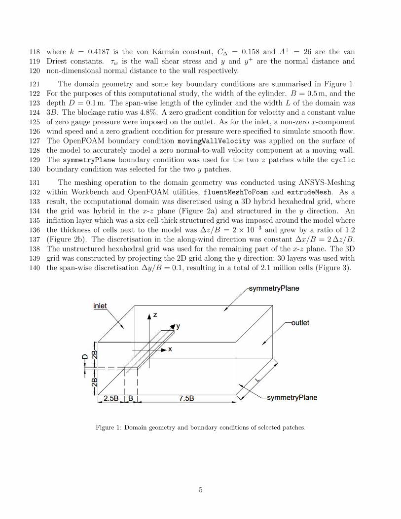
Figure 8 also indicates some influence of the span-wise discretisation on the pressure246
distribution. For the time-averaged pressure coefficient Cp (Figure 8a), all four profiles stayed247
within the BARC envelops. The pressure fluctuation inside the separation bubble modelled in248
the four simulations was in good agreement with the BARC statistics. However, the pressure249
recovery region showed more scatter (Figure 8b). The overall trend was that a coarser grid250
predicted higher pressure fluctuation; results from Grids 3 and 4 were about 5% to 30% larger251
than the upper envelop of the BARC statistics.252
Therefore, it is evident that the flow field around the rectangular cylinder was significantly253
affected by the span-wise discretisation. By reducing the discretisation level in this direction,254
i.e. using a larger filtering width, certain small-scale flow features would not be resolved255
properly. This affected the energy flow and energy dissipation of large-scale vortices, which256
eventually influenced the Strouhal number and the surface pressure distribution. These257
observations were agreed by arguments of Celik et al. (2005) that the mesh convergence of258
LES is impossible to achieve. Both numerical errors associated when resolving most-energetic259
eddies and SGS errors when modelling SGS eddies depend on the filtering width or, in this260
case, the cell size. A decrease in the cell size gradually reduces these errors; eventually, the261
mesh convergence is achieved when the cell size becomes so small that LES simulation is262
equivalent to Direct Numerical Simulation. In addition, there is a limitation on this mesh263
sensitivity study that only cells in the span-wise direction were refined, while cells in the264
x-z plane remained unchanged. This means that the refinement produced more positive265
effects on the fluid solutions on the y direction more than those on the x and z directions.266
This issue was more pronounced in case of high aspect-ratio cells such as those used in this267
computational study.268
11

Table 1: Computational grids in the mesh sensitivity study.
Grid ∆y/B Number of layersG1 0.01 300G2 0.02 150G3 0.04 75G4 0.1 30
4 5 6 7 8 9 10
10-3
0.5
0.52
0.54
0.56
0.58
0.6
0.62
0.64
0.66
Figure 7: Variability of the Strouhal number, St, against the quantity (∆x∆y ∆z)1/3/B, which is the nor-malised filtering width applied to solve fluid solutions in the region next to the model.
12
(a)
0.5 0.7 0.9 1.1 1.3 1.5 1.7 1.9 2.1 2.3 2.5 2.7 2.9 3.1 3.3 3.5 3.7 3.9 4.1 4.3 4.5 4.7 4.9 5.1 5.3 5.5
-1
-0.9
-0.8
-0.7
-0.6
-0.5
-0.4
-0.3
-0.2
-0.1
(b)
0.5 0.7 0.9 1.1 1.3 1.5 1.7 1.9 2.1 2.3 2.5 2.7 2.9 3.1 3.3 3.5 3.7 3.9 4.1 4.3 4.5 4.7 4.9 5.1 5.3 5.50
0.05
0.1
0.15
0.2
0.25
0.3
0.35
0.4
0.45
Figure 8: The surface distribution of (a) the time-averaged pressure coefficient Cp and (b) the standarddeviation of the time-varying pressure coefficient C ′p in comparison to the BARC summary statistics of CFDsimulations (Bruno et al., 2014).
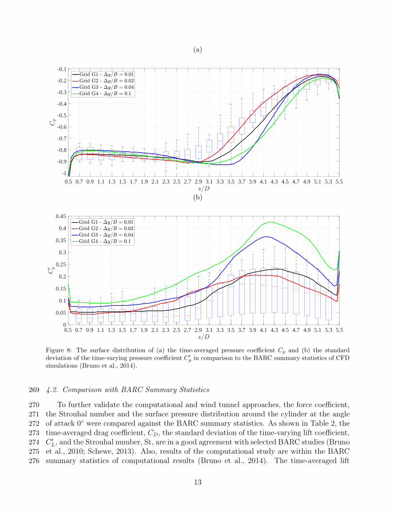
4.2. Comparison with BARC Summary Statistics269
To further validate the computational and wind tunnel approaches, the force coefficient,270
the Strouhal number and the surface pressure distribution around the cylinder at the angle271
of attack 0◦ were compared against the BARC summary statistics. As shown in Table 2, the272
time-averaged drag coefficient, CD, the standard deviation of the time-varying lift coefficient,273
C ′L, and the Strouhal number, St, are in a good agreement with selected BARC studies (Bruno274
et al., 2010; Schewe, 2013). Also, results of the computational study are within the BARC275
summary statistics of computational results (Bruno et al., 2014). The time-averaged lift276
13
Table 2: Comparison of force coefficients and Strouhal number obtained from computational and wind tunnelstudies; (?) numbers in the brackets are the standard deviation of computational results reported in BARC.
Re St CD CL C ′L
CFD study6700 0.608 0.241 -0.056 0.08113000 0.600 0.206 -0.059 0.07527000 0.609 0.206 -0.063 0.059
WT study
20800 0.640 0.225 -0.0811 0.078431200 0.621 0.230 -0.0684 0.084841600 0.622 0.240 -0.0690 0.093252000 0.601 0.252 -0.0706 0.115
WT study6000 – 40000 0.555 0.242 ∼ 0 ∼ 0.08
(Schewe, 2013)CFD study
40000 0.575 0.206 – ∼ 0.146(Bruno et al., 2010)
BARC statistics of CFD(?)
–0.545 0.2148 -0.00282 0.130
(Bruno et al., 2014) (0.075) (0.0258) (0.0284) (0.0748)
coefficient, CL, however displays the largest deviation from the BARC data. Issues regarding277
the accurate setting up angles of attack and correcting the blockage ratio were the major278
contribution to errors in the wind tunnel study. For the computational study, the negative279
CL indicated an asymmetric flow field around the cylinder. This could be attributed to the280
use of the unstructured grid where the cell density and cell size were slightly different between281
the top and bottom halves of the domain.282
Another useful measure of the quality of the experimental measurements and numerical283
predictions are the surface pressure correlation measured along the leading and trailing edges284
and the surface pressure distribution. In Figure 9, despite different Reynolds numbers, the285
pressure correlation obtained from the static simulations and wind tunnel static tests show286
similar trends and reasonably agree with the BARC summary statistics and a selected wind287
tunnel test of Ricciardelli and Marra (2008). The use of the cyclic boundary condition on288
the y patches is thought to increase the pressure correlation beyond ∆y/B = 0.7 to 0.8; this289
issue was also observed by Mannini et al. (2011). In general, the pressure correlation measured290
along the leading edge is higher than that measured along the trailing edge. These results291
indicated the presence of the separation bubble which was well-defined along the span-wise292
direction in comparison to a highly unsteady flow feature close to the trailing edge.293
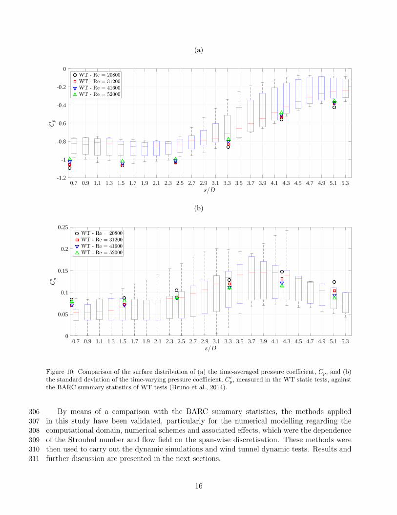
These two flow features can also be inferred from the surface pressure distribution obtained294
from the wind tunnel static tests (Figure 10). The separation bubble close to the leading295
edge was a well correlated recirculating flow feature, which was trapped underneath the shear296
layer generated from the leading edge. The separation bubble induced strong suction, with297
little variation, on the surface of the cylinder (from s/D = 0.7 to 2.5 approximately). Close298
the trailing edge, this shear layer reattached to the surface, leading to a recovery and large299
variation of the surface pressure (from s/D = 3.3 to 4.3 approximately). These flow features300
14

are associated with the impinging vortex shedding phenomenon, which is well documented in301
the literature (Nakamura et al., 1991; Mills et al., 2003; Bruno et al., 2010, 2014). The time-302
averaged pressure coefficient was overestimated due to the blockage ratio issue. Nevertheless,303
a good agreement between results of the wind tunnel static tests and the BARC summary304
statistics can be seen.305
(a)
0 0.1 0.2 0.3 0.4 0.5 0.6 0.7 0.8 0.9 1 1.1 1.2 1.3 1.4 1.5 1.6 1.7 1.8 1.9 2-0.2
0
0.2
0.4
0.6
0.8
1
(b)
0 0.1 0.2 0.3 0.4 0.5 0.6 0.7 0.8 0.9 1 1.1 1.2 1.3 1.4 1.5 1.6 1.7 1.8 1.9 2-0.2
0
0.2
0.4
0.6
0.8
1
Figure 9: Comparison of the surface pressure correlation along (a) the leading edge and (b) the trailing edge,measured in the CFD static simulations and WT static tests, against a selected wind tunnel test and theBARC summary statistics of CFD simulations and WT tests (Bruno et al., 2014).
15
(a)
0.7 0.9 1.1 1.3 1.5 1.7 1.9 2.1 2.3 2.5 2.7 2.9 3.1 3.3 3.5 3.7 3.9 4.1 4.3 4.5 4.7 4.9 5.1 5.3-1.2
-1
-0.8
-0.6
-0.4
-0.2
0
(b)
0.7 0.9 1.1 1.3 1.5 1.7 1.9 2.1 2.3 2.5 2.7 2.9 3.1 3.3 3.5 3.7 3.9 4.1 4.3 4.5 4.7 4.9 5.1 5.30
0.05
0.1
0.15
0.2
0.25
Figure 10: Comparison of the surface distribution of (a) the time-averaged pressure coefficient, Cp, and (b)the standard deviation of the time-varying pressure coefficient, C ′p, measured in the WT static tests, againstthe BARC summary statistics of WT tests (Bruno et al., 2014).
By means of a comparison with the BARC summary statistics, the methods applied306
in this study have been validated, particularly for the numerical modelling regarding the307
computational domain, numerical schemes and associated effects, which were the dependence308
of the Strouhal number and flow field on the span-wise discretisation. These methods were309
then used to carry out the dynamic simulations and wind tunnel dynamic tests. Results and310
further discussion are presented in the next sections.311
16

5. VIV Mechanism of the 5:1 Rectangular Cylinder312
The heaving VIV of the rectangular cylinder was both measured in the wind tunnel and313
modelled computationally while the pitching VIV was measured in the wind tunnel only.314
A comparison of results obtained from these two studies in smooth flow was conducted315
to provide a comprehensive explanation of the VIV mechanism. Using this finding, results316
obtained from the wind tunnel in turbulent flow were then analysed to uncover the mechanism317
of the turbulence-induced effect on the VIV.318
5.1. Heaving VIV319
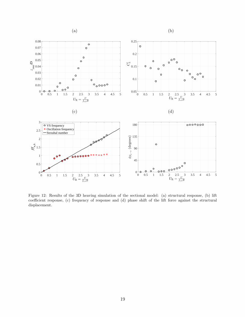
Figures 11 and 12 summarise results as the rectangular cylinder underwent heaving VIV,320
measured in the wind tunnel and 3D heaving simulation respectively. Due to the absence of321
a reliable force measurement during the wind tunnel test, information related to the lift force322
or moment was retrieved by performing the integration of the surface pressure measured at323
the pressure array 4 (Figure 5a). The pressure measurement was associated with certain324
limitation of the sensitivity at low wind speeds; therefore, results of force and moment were325
limited in the this range of wind speeds. Also, the presence of the rolling motion impaired326
results of the vortex shedding frequency and the phase shift of the lift force, which is indicated327
by some fluctuation in Figures 11c and 11d at the reduced wind speed UR = U/(fn,hB) of328
1.4 and 2.5 respectively.329
Results obtained from wind tunnel tests and computational simulations possess similar330
trends. Both studies predicted two VIV lock-in intervals indicated by an increase in the331
structural response and the fact the vortex shedding frequency was locked into the natural332
frequency of the model. Due to the larger Scruton number (higher mass and damping ratio),333
the wind tunnel test predicted lower structural responses during the VIV lock-in compared334
to the ones predicted by the computational simulation.335
In the wind tunnel dynamic test, two heaving VIV lock-in regions occurred at the onset336
reduced wind speed UR,onset = 0.77 and 1.54; the former was smaller in magnitude (Figure337
11a). Similarly, the 3D heaving simulation predicted two VIV lock-in intervals at UR,onset = 1338
and 2 (Figure 12a). The former peak was smaller in magnitude; as was revealed by the339
phase analysis of the surface pressure shown in Figure 13, this peak was associated with two340
vortices alternately being formed on the top or bottom surfaces of the model during one cycle341
of motion. This contrasted with there being only one vortex on the side when the model342
experienced the larger response. This difference in the flow structure could also be observed343
in the instantaneous contour plots of the Q-criterion (Figure 14). The main vortices are344
enclosed by red squares while the blue square highlights the secondary vortex resulted from345
the interaction of the main ones. As suggested by Nakamura et al. (1991) and Matsumoto346
et al. (2008), the number of vortices appearing on one side of the cylinder during one cycle347
of motion, n, is related to the onset reduced wind speed of the VIV heaving lock-in such348
that UR,onset = n/St. This relationship allowed the Strouhal number to be estimated; good349
agreement with results obtained from wind tunnel static tests and static simulation presented350
in Table 2 could be drawn.351
17

(a)
0 1 2 3 4 5 60
0.005
0.01
0.015
0.02
0.025
0.03
(b)
1 1.2 1.4 1.6 1.8 2 2.2 2.4 2.6 2.8 30.12
0.13
0.14
0.15
0.16
0.17
0.18
0.19
Heaving VIV Peak
(c)
0 1 2 3 4 5 60
0.5
1
1.5
2
2.5
3
3.5
4
4.5VS frequencyOscillation frequencyStrouhal number
(d)
1 1.2 1.4 1.6 1.8 2 2.2 2.4 2.6 2.8 30
20
40
60
80
100
120
140
160
180
200
Heaving VIV Peak
Figure 11: Results of the wind tunnel dynamic test of the sectional model restrained to the heaving modeonly: (a) structural response, (b) lift coefficient response, (c) frequency of response and (d) phase shift of thelift force against the structural displacement.
18
(a)
0 0.5 1 1.5 2 2.5 3 3.5 4 4.5 50
0.01
0.02
0.03
0.04
0.05
0.06
0.07
0.08
zrm
s/D
(b)
0 0.5 1 1.5 2 2.5 3 3.5 4 4.5 50.05
0.1
0.15
0.2
0.25
(c)
0 0.5 1 1.5 2 2.5 3 3.5 4 4.5 50
0.5
1
1.5
2
2.5
3
f/f
n,h
VS frequencyOscillation frequencyStrouhal number
(d)
0 0.5 1 1.5 2 2.5 3 3.5 4 4.5 50
45
90
135
180
Figure 12: Results of the 3D heaving simulation of the sectional model: (a) structural response, (b) liftcoefficient response, (c) frequency of response and (d) phase shift of the lift force against the structuraldisplacement.
19

(a) Secondary VIV peak
0 1 2 3 4 5 6s/D
-180
-135
-90
-45
0
45
90
135
180Pressure
phase
angle
(degrees)
CFD Heaving simulationU
R = 1.17
(b) Primary VIV peak
0 1 2 3 4 5 6s/D
-180
-135
-90
-45
0
45
90
135
180
Pressure
phase
angle
(degrees)
CFD Heaving simulationU
R = 3.00
WT Heaving testU
R = 2.15
Figure 13: Phase angles of vortices rolling on the surface of the cylinder measured in the wind tunnel dynamictest and in the 3D heaving simulation; all results are calculated at the reduced wind speeds correspondingthe maximum structural displacement during the lock-in.
(a)
(b)
Figure 14: Contour plots of the Q-criterion Q = 0.1 m s−1 along the mid-span plane at (a) UR = 1.17, i.e.the secondary VIV peak and (b) UR = 3.00, i.e. the primary VIV peak; results were obtained from the 3Dheaving simulation.
20

Both the wind tunnel test and the 3D heaving simulation predicted similar behaviour for352
the phase shift of the lift force against the displacement of the cylinder as shown in Figures353
11d and 12d. As the amplitude of the structural response increased, the in-phase component354
of the lift force became less dominant and after the cylinder reached the lock-out, the lift355
force suddenly became out-of-phase. This transition also indicated that there was a dramatic356
change in the flow structure around the cylinder which was responsible for the lock-out; this357
will be revealed further by analysing the span-wise correlation of the surface pressure as the358
heaving VIV lock-in occurred.359
Concentrating on the primary peak of the heaving VIV measured in the wind tunnel360
dynamic test, the variation of the span-wise pressure correlation around the leading edge361
(Positions A and B) and around the trailing edge (Positions C and D) is illustrated in362
Figure 15; the locations of these four positions are indicated in Figure 5b. Before the lock-363
in occurred, the pressure correlation around the leading edge was higher than that around364
the trailing edge, illustrating the presence of the leading edge vortex. The increase in the365
amplitude of the response improved the correlation of the surface pressure. However, during366
the lock-in, the correlation level around Position C was higher than those around the leading367
edge. This result indicated a strongly correlated flow feature occurred at Position C every368
cycle of the motion and it led to an increase in the response whereas the motion-induced369
leading-edge vortex was only responsible for triggering the motion. It was noticed that the370
span-wise pressure correlation exhibited an increase at ∆y/B = 1. This was caused the371
rolling motion of the cylinder, coupling with a finite span-wise length of the model and the372
end plates, which resulted in a standing wave effect superimposed on the flow field.373
Results obtained from the heaving simulation also revealed similar behaviour (Figure 16).374
Before the VIV lock-in (UR = 1.67), the flow field around the leading edge was better corre-375
lated than the one around the trailing edge. When the lock-in occurred and the amplitude376
of the response increased (UR = 2.00 to 2.67) and reached the peak (UR = 3.00), a slight377
decrease in the correlation level around the leading edge was observed while, around the378
trailing edge, the flow field was better correlated. When the system reached the lock-out,379
the correlation level around the trailing edge suddenly decreased.380
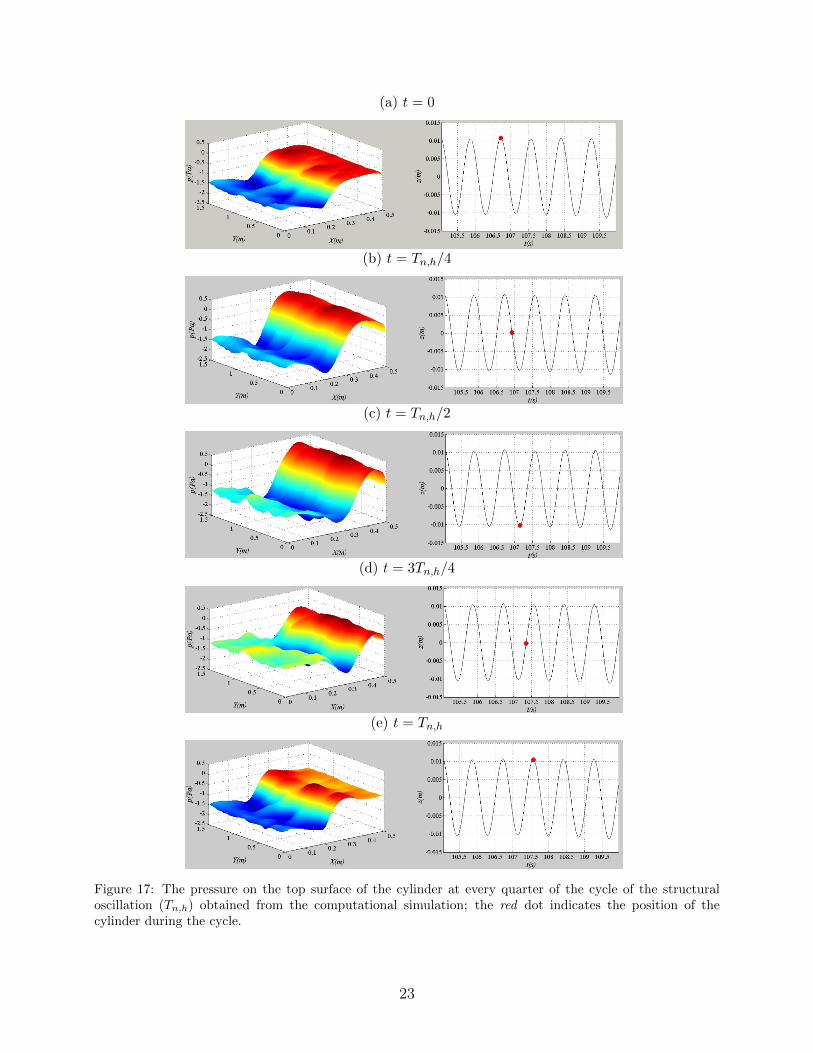
Figure 17 describes the variation of the pressure field on the top surface at UR = 3.00381
during one cycle of the structural motion (Tn,h) extracted from the computational simulation.382
The pressure field presented here is the dominant component resulted from a Proper Orthog-383
onal Decomposition analysis. At the start of the cycle of structural motion t = 0, there was384
a vortex being shed from the leading edge; the downward motion of the cylinder from t = 0385
to Tn,h/2, however, significantly affected its span-wise geometry, degrading its span-wise cor-386
relation and causing it to propagate downstream. In the next quarter of the cycle, due to the387
upward accelerating movement of the cylinder, this motion-induced leading-edge vortex dra-388
matically slowed down and appeared to impinge on the surface of the cylinder. During this389
process, this vortex gained strength and its span-wise correlation improved; this increased390
the lift force acting on the cylinder in the direction such that the cylinder was effectively391
brought back to the equilibrium position. In the final quarter of the cycle, thanks to the392
decelerating upward motion of the cylinder, this vortex was pushed downstream at a higher393
rate and was eventually shed into the wake. The behaviour of the motion-induced leading-394
21

edge vortex during one cycle of the heaving motion is summarised in Figure 18. Together the395
wind tunnel dynamic test, these results from the computational simulation indicated that,396
particularly for the 5:1 rectangular cylinder, the motion-induced leading-edge vortex acted397
as a triggering mechanism for the VIV response while the impingement of this vortex on398
the surface of the cylinder close to the trailing edge resulted in an increase in the structural399
response during the lock-in.400
(a) UR = 1.76
0 0.5 1 1.5 2 2.5∆y/B
0
0.2
0.4
0.6
0.8
1
COR
p
(b) UR = 1.82
0 0.5 1 1.5 2 2.5∆y/B
0
0.2
0.4
0.6
0.8
1
COR
p
(c) UR = 2.16
0 0.5 1 1.5 2 2.5∆y/B
0
0.2
0.4
0.6
0.8
1
COR
pFigure 15: Wind tunnel results of the span-wise pressure correlation measured at 4 stream-wise positions inthe smooth flow during the heaving VIV lock-in; black : Position A; red : Position B; blue: Position C; green:Position D.
(a) Leading edge (x/B = 0.18)
0 0.5 1 1.5 2 2.5∆y/B
0
0.2
0.4
0.6
0.8
1
COR
p
(b) Trailing edge (x/B = 0.82)
0 0.5 1 1.5 2 2.5∆y/B
0
0.2
0.4
0.6
0.8
1
COR
p
Ur = 1.33
Ur = 1.67
Ur = 2.00
Ur = 2.33
Ur = 2.67
Ur = 3.00
Ur = 3.33
Ur = 3.67
Figure 16: Computational results of variation of the span-wise pressure correlation around the leading andtrailing edges as the cylinder experienced the heaving VIV lock-in; black : before the lock-in; red : VIV lock-in;blue: after the lock-in.
22
(a) t = 0
(b) t = Tn,h/4
(c) t = Tn,h/2
(d) t = 3Tn,h/4
(e) t = Tn,h
Figure 17: The pressure on the top surface of the cylinder at every quarter of the cycle of the structuraloscillation (Tn,h) obtained from the computational simulation; the red dot indicates the position of thecylinder during the cycle.
23

t = 0 t = Tn/2 t = Tn
T1
T1
T1
T1
Impingement of the motion-induced leading edge vortex T1
T1
Figure 18: Schematic illustrating the development of the motion-induced leading edge vortex T1 throughoutone cycle of the heaving motion during the VIV lock-in.
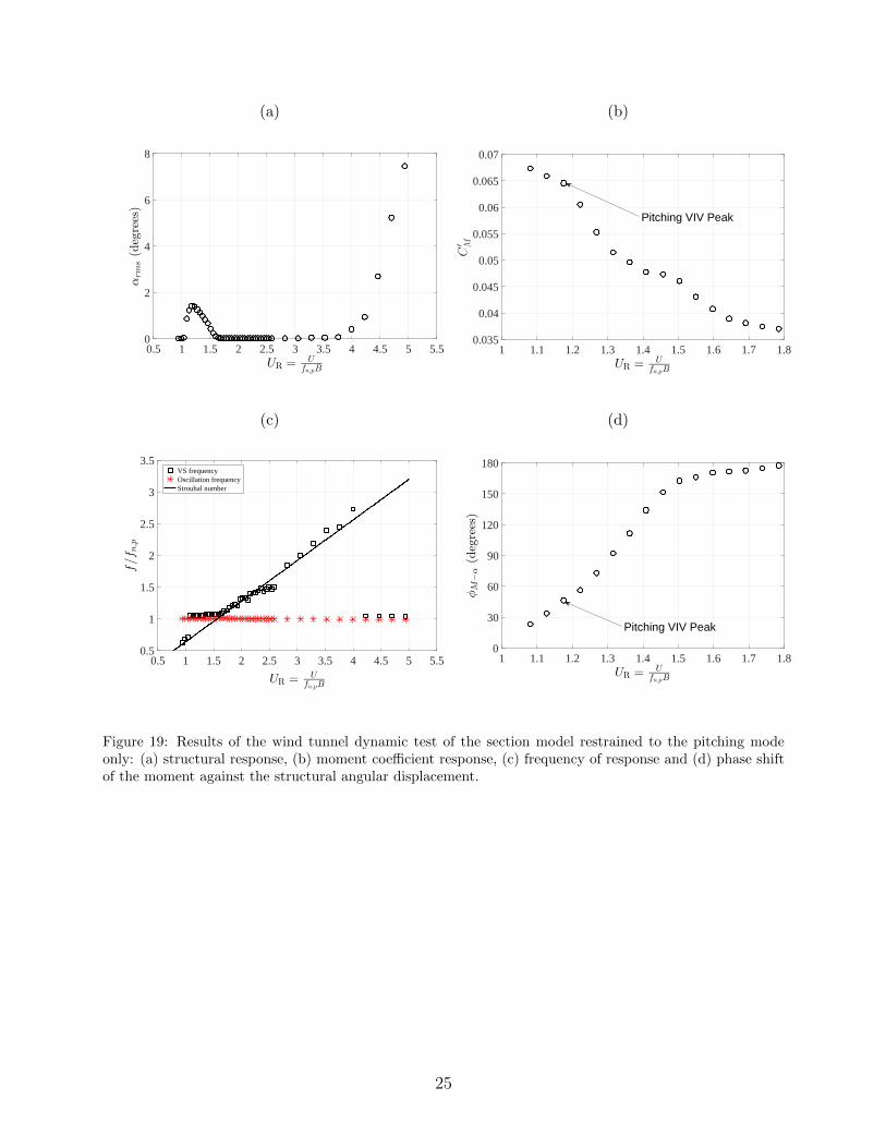
5.2. Pitching VIV401
When the model was restrained to the pitching mode only, two different behaviours402
were observed in Figure 19. The torsional flutter occurred at a high wind speed and was403
characterised by a dramatic increase in the angular displacement. One pitching VIV lock-in404
was observed at the reduced wind speed UR = 1.03. The phase analysis of the surface pressure405
on the top surface revealed there were 1.5 vortices during one cycle of motion (Figure 20)406
or, in other words, it took 1.5 cycles of motion for one vortex created at the leading edge to407
reach the trailing edge and then be shed into the wake. Based on Matsumoto et al. (2008),408
this corresponded to the secondary VIV peak; the primary VIV peak did not appear as was409
also found by Nakamura and Nakashima (1986). In comparison to the heaving response, as410
the wind speed increased, the angular response was seen to rise quite suddenly and, beyond411
the peak, it only gradually decreased. Analysing the phase shift of the moment against the412
angular displacement revealed a more gradual change in the phase angle during the lock-in.413
24
(a)
0.5 1 1.5 2 2.5 3 3.5 4 4.5 5 5.5UR = U
fn,pB
0
2
4
6
8
αrms(degrees)
(b)
1 1.1 1.2 1.3 1.4 1.5 1.6 1.7 1.8UR =
Ufn,pB
0.035
0.04
0.045
0.05
0.055
0.06
0.065
0.07
C′ M
Pitching VIV Peak
(c)
0.5 1 1.5 2 2.5 3 3.5 4 4.5 5 5.5
UR =U
fn,pB
0.5
1
1.5
2
2.5
3
3.5
f/f n
,p
VS frequencyOscillation frequencyStrouhal number
(d)
1 1.1 1.2 1.3 1.4 1.5 1.6 1.7 1.8UR = U
fn,pB
0
30
60
90
120
150
180φM
−α(degrees)
Pitching VIV Peak
Figure 19: Results of the wind tunnel dynamic test of the section model restrained to the pitching modeonly: (a) structural response, (b) moment coefficient response, (c) frequency of response and (d) phase shiftof the moment against the structural angular displacement.
25

0 1 2 3 4 5 6s/D
-180
-150
-120
-90
-60
-30
0
30
60
90
120
150
180
Pressure
phase
angle
(degrees)
Figure 20: Phase angles of vortices rolling on the surface of the cylinder experiencing the pitching VIVresponse, measured in the wind tunnel dynamic test at UR = 1.17, i.e. at the pitching VIV peak.
The variation of the surface pressure correlation measured along the leading edge (Po-414
sitions A and B) and along the trailing edge (Positions C and D) during the pitching VIV415
lock-in is summarised in Figure 21. In comparison to what was observed when the cylinder416
was restrained to the heaving mode only, certain similarities can be drawn. After the max-417
imum structural response was reached, a reduction in the pressure correlation occurred at418
Position C and led to a decrease in the amplitude of the structural response. Knowing the419
phase shift between the surface pressure and the angular displacement, the development of420
the flow field around the cylinder during two successive cycles of the motion is illustrated421
in Figure 22. After one cycle of motion, the motion-induced leading-edge vortex travelled422
downstream a distance up to two-thirds of the width of the cylinder. In the next quarter of423
the cycle, the upward accelerating motion of the trailing edge caused this vortex to impinge424
on the surface, leading to a rise in the moment acting on the cylinder. Afterwards, the425
motion of the cylinder slowed down; the vortex was pushed towards the trailing edge and426
eventually shed into the wake. This result highlighted the different role of the motion-induced427
leading-edge vortex and its impingement in the VIV of the 5:1 rectangular cylinder.428
26

(a) UR = 1.13
0 0.5 1 1.5 2 2.5∆y/B
0
0.2
0.4
0.6
0.8
1
COR
p(b) UR = 1.22
0 0.5 1 1.5 2 2.5∆y/B
0
0.2
0.4
0.6
0.8
1
COR
p
(c) UR = 1.60
0 0.5 1 1.5 2 2.5∆y/B
0
0.2
0.4
0.6
0.8
1
COR
p
Figure 21: Wind tunnel results of the span-wise pressure correlation measured at 4 stream-wise positions inthe smooth flow during the pitching VIV lock-in; black : Position A; red : Position B; blue: Position C; green:Position D.
t = 0 t = Tn/2 t = Tn t = 3Tn/2
T1
T1
T1
T1
T1
T1
T1
Impingement of the motion-induced leading edge vortex T1
Figure 22: Schematic illustrating the development of the motion-induced leading-edge vortex T1 throughout1.5 cycles of the pitching motion during the VIV lock-in.
27
6. Conclusion429
By analysing the surface pressure correlation along the leading edge and trailing edge430
and investigating the flow field offered by the computational simulation, this paper presents a431
comprehensive explanation of the VIV mechanism of the 5:1 rectangular cylinder. Regardless432
of being restrained to the heaving mode only or the pitching mode only, there were two433
key flow features which were important for the VIV of this particular geometry. The first434
one was the leading-edge vortex, which was responsible for triggering the motion, resulting435
in some initial structural displacement at the start of the lock-in. The second one was436
the impingement of the motion-induced leading-edge vortex on the surface of the cylinder,437
occurring close to the trailing edge. This flow feature led to a rise in the suction and in the lift438
force or moment acting on the cylinder, causing an increase in the structural response during439
the lock-in. As part of a boarder wind tunnel and computational studies, these outcomes440
will be analysed to provide more insight into the turbulence-induced effect of the VIV of a441
5:1 rectangular cylinder; further results and discussion will be presented in a separate paper.442
There were a number of limitations to the work presented in this paper. As for CFD443
simulations, the use of finer computational domains particularly in the span-wise direction is444
of importance to minimise issues related to the mesh sensitivity. In addition, experimental445
errors were observed in WT dynamic tests; the combination of the end plates, the finite span-446
wise length of the model and its rolling oscillation caused some resonance effect limiting the447
usability of the pressure data to investigate the span-wise correlation. This issue should be448
studied and a standard guideline to perform dynamic wind tunnel tests should be produced449
Acknowledgements450
The work presented here was supported by the University of Nottingham through the451
Dean of Engineering Research Scholarship for International Excellence, the access to the452
Atmospheric Boundary Layer wind tunnel and the High Performance Computer. The authors453
wish to express their sincere thanks to technicians in the Department of Civil Engineering454
during wind tunnel tests.455
References456
Bai, Y., Yang, K., Sun, D., Zhang, Y., Kennedy, D., Williams, F., Gao, X., 2013. Numerical457
aerodynamic analysis of bluff bodies at a high Reynolds number with three-dimensional458
CFD modelling. Science China: Physics, Mechanics and Astronomy 56, 277 – 289.459
Batina, J., 1990. Unsteady Euler airfoil solutions using unstructured dynamic meshes. AIAA460
Journal 28 (8), 1381 – 1388.461
Bruno, L., Coste, N., Fransos, D., 2011. Simulated flow around a rectangular 5:1 cylinder:462
Spanwise discretisation effects and emerging flow features. Journal of Wind Engineering463
and Industrial Aerodynamics 104 – 106 (0), 203 – 215.464
28
Bruno, L., Fransos, D., Coste, N., Bosco, A., 2010. 3D flow around a rectangular cylinder: A465
computational study. Journal of Wind Engineering and Industrial Aerodynamics 98, 263466
– 276.467
Bruno, L., Salvetti, M., Ricciardelli, F., 2014. Benchmark on the Aerodynamics of a Rect-468
angular 5:1 Cylinder: An overview after the first four years of activity. Journal of Wind469
Engineering and Industrial Aerodynamics 126 (0), 87 – 106.470
Cao, S., 2015. Towards better understanding of bridge aerodynamics - turbulence effects. In:471
The 14th International Conference on Wind Engineering. Porto Alegre, Brazil.472
Celik, I., Ghia, U., Roaches, P., Freitas, C., Coleman, H., Raad, P., 2008. Procedure for473
estimation and reporting of uncertainty due to discretisation in CFD applications. Journal474
of Fluids Engineering 130 (7).475
Celik, I. B., Cehreli, Z. N., Yavuz, I., 2005. Index of resolution quality for Large Eddy476
Simulation. Journal of Fluids Engineering 127 (5), 949 – 958.477
Daniels, S., Castro, I., Xie, Z., 2014. Free-stream turbulence effects on bridge decks undergoing478
vortex-induced vibrations using Large-Eddy Simulation. In: The 11th UK Conference on479
Wind Engineering. Birmingham, UK.480
Furby, C., Tabor, G., Weller, H., Gosman, A., 1997. A comparative study of subgrid scale481
models in homogeneous isotropic trubulence. Physics of Fluids (1994 – present) 9 (5), 1416482
– 1429.483
Goswami, I., Scanlan, R., Jones, N., 1993. Vortex-induced vibration of circular cylinder.484
Journal of Engineering Mechanics 11, 2270 – 2287.485
Kareem, A., Wu, T., 2013. Wind-induced effects on bluff bodies in turbulent flows: Nonsta-486
tionary, non-Gaussian and nonlinear features . Journal of Wind Engineering and Industrial487
Aerodynamics 122 (0), 21 – 37, the Seventh International Colloquium on Bluff Body Aero-488
dynamics and Applications (BBAA7).489
Kawatani, M., Kim, H., Uejima, H., Kobayashi, H., 1993. Effects of turbulence flows on490
vortex-induced oscillation of bridge girders with basic sections. Journal of Wind Engineer-491
ing and Industrial Applications 49 (1 – 3), 477 – 486.492
Kawatani, M., Toda, N., Sato, M., Kobayashi, H., 1999. Vortex-induced torsional oscillations493
of bridge girders with basic sections in turbulent flows. Journal of Wind Engineering and494
Industrial Applications 83 (1 – 3), 327 – 336.495
Kobayashi, H., Kawatani, M., Kim, H., 1992. Effects of turbulence characteristics on vortex-496
induced oscillation of rectangular cylinders. Journal of Wind Engineering and Industrial497
Applications 41, 775 – 784.498
Kobayashi, H., Kawatani, M., Nakade, O., 1990. Vortex-induced oscillations of two dimen-499
sional rectangular cylinders in large scale turbulence. Journal of Wind Engineering and500
Industrial Applications 33 (1 – 2), 101 – 106.501
29

Larsen, A., Walther, J., 1998. Discrete vortex simulation of flow around five generic bridge502
deck sections. Journal of Wind Engineering and Industrial Aerodynamics 77 – 78, 591 –503
602.504
Lee, B., 1975. The effects of turbulence on the surface pressure field of a square prism. Journal505
of Fluid Mechanics 69 (2), 263 – 282.506
Mannini, C., Soda, A., Schewe, G., 2011. Numerical investigation on the three-dimensional507
unsteady flow past a 5:1 rectangular cylinder. Journal of Wind Engineering and Aerody-508
namics 99 (4), 469 – 482.509
Matsumoto, M., Shiraishi, N., Shirato, H., Stoyanoff, S., Yagi, T., 1993. Mechanism of, and510
turbulence effect on vortex-induced oscillations for bridge box girders. Journal of Wind511
Engineering and Industrial Aerodynamics 49 (1 – 3), 467 – 478.512
Matsumoto, M., Shirato, H., Araki, K., Haramura, T., Hashimoto, T., 2003. Spanwise co-513
herence characteristics of surface pressure field on 2D bluff bodies. Journal of Wind Engi-514
neering and Industrial Aerodynamics 91 (1 – 2), 155 – 163.515
Matsumoto, M., Yagi, T., Tamaki, H., Tsubota, T., 2008. Vortex-induced vibration and its516
effect on torsional flutter instability in the case of B/D = 4 rectangular cylinder. Journal517
of Wind Engineering and Industrial Aerodynamics 96 (6 – 7), 971 – 983.518
Mills, R., Sheridan, J., Hourigan, K., 2003. Partical Image Velocimetry and visualisation of519
natural and forced flow around rectangular. Journal of Wind and Mechanics 478, 299 –520
323.521
Nakamura, Y., Nakashima, M., 1986. Vortex excitation of prisms with elongated rectangular,522
H and T-cross-sections. Journal of Fluids and Structures 163, 149 – 169.523
Nakamura, Y., Ohya, Y., Tsuruta, H., 1991. Experiments on vortex shedding from flat plates524
with square leading and trailing edges. Journal of Fluid Engineering 222, 473 – 447.525
Ohya, Y., Nakamura, Y., Ozono, S., Tsuruta, H., 1992. A numerical study of vortex shedding526
from flat plates with square leading and trailing edges. Journal of Fluid Mechanics 236,527
445 – 460.528
Owen, J., Hargreaves, D., Gu, X., 2006. Modelling the Mechanism of Vortex Induced Response529
of Bridge Deck. In: The 7th UK Conference on Wind Engineering (WES 06). Glasgow.530
Ozono, S., Ohya, Y., Nakamura, Y., Nakayama, R., 1992. Stepwise increase in the Strouhal531
number for flows around flat plates. International Journal for Numerical Methods in Fluid532
15 (9), 1025 – 1036.533
Ricciardelli, F., Marra, A., 2008. Sectional aerodynmic forces and their longitudinal correla-534
tion on a vibrating 5:1 rectangular cylinder. In: BBAA VI International Colloquium on:535
Bluff Bodies Aerodynamics and Applications. Milano, Italy.536
Roache, P., 1997. Quantification of uncertainty in computational fluid dynamics. Annual537
Reviews of Fluid Mechanics 29, 123 – 160.538
30

Schewe, G., 2013. Reynolds-number-effect in flow around a rectangular cylinder with aspect539
ratio 1:5. Journal of Fluids and Structures 36 (0), 16 – 25.540
Sun, D., Owen, J., Wright, N., 2009. Application of the k-ω turbulence model for a wind-541
induced vibration study of 2D bluff bodies. Journal of Wind Engineering and Industrial542
Aerodynamics 97 (2).543
Sun, D., Owen, J., Wright, N., Liaw, K., 2008. Fluid-structure interaction of prismatic line-544
like structure, using LES and block-iterative coupling. Journal of Wind Engineering and545
Industrial Aerodynamics 96 (6 – 7).546
Tan, B., Thompson, M., Hourigan, K., 1998. Simulated flow around long plates under cross547
flow pertubations. International Journal of Fluid Dynamics 2 (1).548
Waterson, N., Baker, N., 2010. Numerical Prediction of Flutter Behaviour for Long-span549
Bridge Decks. In: The 5th International Symposium on Computational Wind Engineering550
(CWE2010). North Carolina, USA.551
Wu, T., Kareem, A., 2012. An overview of vortex-induced vibration (VIV) of bridge decks.552
Journal of Frontiers of Structural and Civil Engineering 6 (64), 335 – 347.553
Xiang, H., Ge, Y., 2002. Refinements on aerodynamic stability analysis of super long-span554
bridge. Journal of Wind Engineering and Industrial Aerodynamics 90 (12 – 15), 1493 –555
1515, fifth Asia-Pacific Conference on Wind Engineering.556
Zhu, Z., Chen, Z., 2013. Large eddy simulation of aerodynamics of a flat box girder on557
long-span bridges. Procedia Engineering 61, 212 – 219.558
31
Recommended