BULLETIN (New Series) OF THEAMERICAN MATHEMATICAL SOCIETYVolume 45, Number 4, October 2008, Pages 535–593S 0273-0979(08)01212-3Article electronically published on June 25, 2008
VARIATIONAL METHODSIN RELATIVISTIC QUANTUM MECHANICS
MARIA J. ESTEBAN, MATHIEU LEWIN, AND ERIC SERE
Abstract. This review is devoted to the study of stationary solutions of lin-ear and nonlinear equations from relativistic quantum mechanics, involving theDirac operator. The solutions are found as critical points of an energy func-tional. Contrary to the Laplacian appearing in the equations of nonrelativisticquantum mechanics, the Dirac operator has a negative continuous spectrumwhich is not bounded from below. This has two main consequences. First, theenergy functional is strongly indefinite. Second, the Euler-Lagrange equations
are linear or nonlinear eigenvalue problems with eigenvalues lying in a spectralgap (between the negative and positive continuous spectra). Moreover, sincewe work in the space domain R3, the Palais-Smale condition is not satisfied.For these reasons, the problems discussed in this review pose a challenge in theCalculus of Variations. The existence proofs involve sophisticated tools fromnonlinear analysis and have required new variational methods which are nowapplied to other problems.
In the first part, we consider the fixed eigenvalue problem for models of afree self-interacting relativistic particle. They allow us to describe the localizedstate of a spin-1/2 particle (a fermion) which propagates without changingits shape. This includes the Soler models, and the Maxwell-Dirac or Klein-Gordon-Dirac equations.
The second part is devoted to the presentation of min-max principles allow-ing us to characterize and compute the eigenvalues of linear Dirac operatorswith an external potential in the gap of their essential spectrum. Many con-sequences of these min-max characterizations are presented, among them arenew kinds of Hardy-like inequalities and a stable algorithm to compute theeigenvalues.
In the third part we look for normalized solutions of nonlinear eigenvalueproblems. The eigenvalues are Lagrange multipliers lying in a spectral gap.We review the results that have been obtained on the Dirac-Fock model whichis a nonlinear theory describing the behavior of N interacting electrons in anexternal electrostatic field. In particular we focus on the problematic definition
of the ground state and its nonrelativistic limit.In the last part, we present a more involved relativistic model from Quan-
tum Electrodynamics in which the behavior of the vacuum is taken into ac-count, it being coupled to the real particles. The main interesting feature ofthis model is that the energy functional is now bounded from below, providingus with a good definition of a ground state.
Received by the editors June 22, 2007.2000 Mathematics Subject Classification. Primary 49S05, 35J60, 35P30, 35Q75, 81Q05, 81V70,
81V45, 81V55.Key words and phrases. Relativistic quantum mechanics, Dirac operator, variational methods,
critical points, strongly indefinite functionals, nonlinear eigenvalue problems, ground state, non-relativistic limit, Quantum Chemistry, mean-field approximation, Dirac-Fock equations, Hartree-Fock equations, Bogoliubov-Dirac-Fock method, Quantum Electrodynamics.
c©2008 American Mathematical SocietyReverts to public domain 28 years from publication
535

536 MARIA J. ESTEBAN, MATHIEU LEWIN, AND ERIC SERE
Contents
Introduction 536Notations and basic properties of the Dirac operator 5411. Nonlinear Dirac equations for a free particle 5421.1. Soler models: Existence by O.D.E. techniques 5431.2. Soler models: Existence by variational techniques 5441.3. Existence of solutions by perturbation theory 5451.4. Nonlinear Dirac equations in the Schwarzschild metric 5461.5. Solutions of the Maxwell-Dirac equations 5461.6. Nonlinear Dirac evolution problems 5512. Linear Dirac equations for an electron in an external field 5522.1. A variational characterization of the eigenvalues of Dc + V 5532.2. Numerical method based on the min-max formula 5592.3. New Hardy-like inequalities 5602.4. The nonrelativistic limit 5612.5. Introduction of a constant external magnetic field 5623. The Dirac-Fock equations for atoms and molecules 5633.1. The (nonrelativistic) Hartree-Fock equations 5633.2. Existence of solutions to the Dirac-Fock equations 5643.3. Nonrelativistic limit and definition of the Dirac-Fock “ground state” 5684. The mean-field approximation in Quantum Electrodynamics 5704.1. Definition of the free vacuum 5734.2. The Bogoliubov-Dirac-Fock model 5754.3. Global minimization of Eν
BDF: The polarized vacuum 5794.4. Minimization of Eν
BDF in charge sectors 5804.5. Neglecting vacuum polarization: Mittleman’s conjecture 583References 587
Introduction
In this paper we present various recent results concerning some linear and non-linear variational problems in relativistic quantum mechanics involving the Diracoperator.
Dirac derived his operator in 1928 [44] starting from the usual classical expressionof the energy of a free relativistic particle of momentum, p ∈ R
3, and mass m,
(1) E2 = c2|p|2 + m2c4,
where c is the speed of light, and imposing the necessary relativistic invariances.By means of the usual identification,
p ←→ −i∇,
where is Planck’s constant, he found that an adequate observable for describ-ing the energy of the free particle should therefore be a self-adjoint operator Dc
satisfying the equation
(2) (Dc)2 = −c2
2∆ + m2c4.

VARIATIONAL METHODS IN RELATIVISTIC QUANTUM MECHANICS 537
Taking the locality principle into account, Dirac proposed looking for a local oper-ator which is of the first order with respect to p = −i∇:
(3) Dc = −ic α · ∇ + mc2β = −ic3∑
k=1
αk∂k + mc2β,
where α1, α2, α3 and β are Hermitian matrices that have to satisfy the anticom-mutation relations
(4)
⎧⎨⎩ αkα + ααk = 2 δk ,αkβ + βαk = 0,
β2 = .
It can be proved [159] that the smallest dimension in which the relations in (4) cantake place is 4 (i.e. α1, α2, α3 and β should be 4× 4 hermitian matrices), meaningthat Dc has to act on L2(R3, C4). The usual representation in 2× 2 blocks is givenby
β =(
I2 00 −I2
), αk =
(0 σk
σk 0
)(k = 1, 2, 3) ,
where the Pauli matrices are defined as
σ1 =(
0 11 0
), σ2 =
(0 −ii 0
), σ3 =
(1 00 −1
).
By (1) the time-dependent Dirac equation describing the evolution of a freeparticle is
(5) i∂
∂tΨ = DcΨ.
This equation has been successfully used in physics to describe relativistic particleshaving a spin-1/2.
The main unusual feature of the Dirac equation is the spectrum of Dc which isnot bounded from below:
(6) σ(Dc) = (−∞,−mc2] ∪ [mc2,∞).
Compared with nonrelativistic theories in which the Schrodinger operator −∆/(2m)appears instead of Dc, property (6) leads to important physical, mathematical andnumerical difficulties. Indeed, if one simply replaces −∆/(2m) by Dc in the energiesor operators that are commonly used in the nonrelativistic case, one obtains energieswhich are not bounded from below.
Although there is no observable electron of negative energy, the negative spec-trum plays an important role in physics. Dirac himself suspected that the negativespectrum of his operator could generate new interesting physical phenomena, andin the 1930’s he proposed the following interpretation [45, 46, 47]:
“We make the assumption that, in the world as we know it, nearlyall the states of negative energy for the electrons are occupied, withjust one electron in each state, and that a uniform filling of all thenegative-energy states is completely unobservable to us.” [47]
Physically, one therefore has to imagine that the vacuum (called the Dirac sea) isfilled with infinitely many virtual particles occupying the negative energy states.With this conjecture, a real free electron cannot be in a negative state due to thePauli principle which forbids it to be in the same state as a virtual electron of theDirac sea.

538 MARIA J. ESTEBAN, MATHIEU LEWIN, AND ERIC SERE
With this interpretation, Dirac was able to conjecture the existence of “holes” inthe vacuum, interpreted as “anti-electrons” or positrons, having a positive chargeand a positive energy. The positron was discovered in 1932 by Anderson [3]. Diracalso predicted the phenomenon of vacuum polarization: in the presence of an electricfield, the virtual electrons are displaced, and the vacuum acquires a nonconstantdensity of charge. All these phenomena are now well known and well establishedin physics. They are direct consequences of the existence of the negative spectrumof Dc, showing the crucial role played by Dirac’s discovery.
Actually, in practical computations it is quite difficult to deal properly with theDirac sea. As a consequence the notion of “ground state” (the state of “lowestenergy” which is supposed to be the most “stable” for the system under consider-ation) is problematic for many of the models found in the literature. Numerically,the unboundedness from below the spectrum is also the source of important practi-cal issues concerning the convergence of the algorithms considered, or the existenceof spurious (unphysical) solutions.
Dirac’s interpretation of the negative energies will be an implicit assumptionthroughout this review in the sense that we shall (almost) always look for positiveenergy solutions for the electrons. In the last section, we present a model fromQuantum Electrodynamics (QED) in which the nonlinear behavior of the Dirac seawill be fully taken into account.
Mathematically, most of the energy functionals that we shall consider are stronglyindefinite: they are unbounded from below and all their critical points have an in-finite Morse index. Note that the mathematical methods allowing us to deal withstrongly indefinite functionals have their origin in the works of P. Rabinowitz con-cerning the study of nonlinear waves [134] and also the study of periodic solutionsof Hamiltonian systems [135]. Many results have followed these pioneering works,and powerful theories have been devised, in particular in the field of periodic orbitsof Hamiltonian systems: the linking theorem of Benci and Rabinowitz [17], Clarkeand Ekeland’s dual action functional [39], Conley and Zehnder’s relative index [41],Floer’s homology [74], etc.
Another difficulty with the models presented in this review is the lack of com-pactness: the Palais-Smale condition is not satisfied due to the unboundedness ofthe domain R
3. Variational problems with lack of compactness also have beenextensively studied. Let us mention the work of Sacks and Uhlenbeck [145] onharmonic maps, Lieb’s Lemma [114], Brezis and Nirenberg’s study of elliptic PDEswith critical exponents [25], the concentration-compactness method of P.-L. Lions[118], Bahri and Coron’s critical points at infinity [10], and more recently Fang andGhoussoub’s Palais-Smale sequences with Morse information [68, 77].
The combination of the two types of difficulties above poses a challenge in theCalculus of Variations. To prove the results presented in this review, it has beennecessary to adapt some of the sophisticated tools mentioned above and to introducenew ideas. The novel variational methods that we have designed can be appliedin general situations and in particular in the study of crystalline matter (nonlinearSchrodinger equations with periodic potentials).
The review contains four different parts which are almost independent. Thecommon feature of all the problems addressed in this review is the variational studyof linear and nonlinear eigenvalue problems with eigenvalues in spectral gaps. Inthe nonlinear case, there are two different classes of problems. Either we fix the

VARIATIONAL METHODS IN RELATIVISTIC QUANTUM MECHANICS 539
eigenvalue and let the L2-norm of the solutions free, or we look for normalizedsolutions. The eigenvalue is then a Lagrange multiplier which has to stay in thespectral gap.
In the first section, we describe the results that have been obtained for somemodels describing one self-interacting free relativistic spin-1/2 particle. The sim-plest case is when the interaction is “local”, i.e. represented by a nonlinear functionF of the spinor ψ(t, x) of the particle. The general form for the equations that weconsider in this part is
Dcψ − ωψ = ∇F (ψ).These models are phenomenological. A Lorentz-invariant interaction term F (ψ) ischosen in order to find a model of the free localized electron (or on another spin-1/2particle), which fits with experimental data (see [138]).
At the end of the first section, we present two nonlocal models: the Maxwell-Dirac and the Klein-Gordon-Dirac equations in which the electron interacts with itsown electromagnetic field. The Maxwell-Dirac equations take the following form:⎧⎨⎩ (Dc + v − α · A)ψ = ωψ,
−4π∆v = |ψ|2,−4π∆Ak = (ψ, αkψ) , k = 1, 2, 3.
From a mathematical viewpoint, the equations considered in the first section arenonlinear eigenvalue problems, in which the eigenvalue is fixed in a spectral gap,but the L2-norm of the solution is not known. They are the Euler-Lagrange equa-tions of a strongly indefinite functional. Moreover, this functional does not satisfythe Palais-Smale condition and the classical Benci-Rabinowitz linking theorem [17]cannot be applied. The solutions are obtained by a “noncompact” linking argumentinspired by the works of Hofer and Wysocki [93] and Sere [150] on homoclinic orbitsof Hamiltonian systems. An additional difficulty is that the nonlinearity can vanisheven for very large values of ψ, and this makes the a priori bounds on Palais-Smalesequences very delicate.
The second section is devoted to the study of min-max principles allowing us tocharacterize the eigenvalues of Dirac operators with an external potential V in thegap of their essential spectrum. Such operators are commonly used to describe thedynamics of an electron which is subject to the action of an external electrostaticfield with associated potential V (for instance an electron in the field created bya nucleus). It can also be used to describe many noninteracting electrons. Forpotentials V satisfying appropriate assumptions, the spectrum of the perturbedDirac operator Dc + V takes the form
σ(Dc + V ) = (−∞,−mc2] ∪ εii∈N ∪ [mc2,∞),
where the εi’s are eigenvalues of finite multiplicity in (−mc2, mc2), which can onlyaccumulate at the thresholds −mc2 or mc2 (see [18, 19]). The min-max formulaspresented in this section furnish a useful variational characterization of the εi’s andof the associated eigenfunctions:
(Dc + V )ϕi = εiϕi.
The min-max formulas are general and can be used in other settings where eigen-values in a gap of the essential spectrum have to be characterized or computed.Many consequences of the min-max principles are derived in this section, includingan algorithm for the computation of the eigenvalues.

540 MARIA J. ESTEBAN, MATHIEU LEWIN, AND ERIC SERE
In Section 3, we present results concerning the Dirac-Fock model [156], allowingus to describe N interacting electrons in an external electrostatic field. This isa nonlinear model which is used in Quantum Chemistry to compute the state ofsuch electrons in heavy atoms. The energy functional is strongly indefinite andtherefore it is really not obvious how to find an adequate definition of the groundstate and to prove the existence of critical points in general. Explaining how thiscan be achieved is the main goal of the section. The model consists of a system ofN coupled nonlinear equations, posed on L2(R3, C4)N :
Dc,Φ ϕi = εiϕi, 0 < εi < mc2,
whereDc,Φ = Dc + V + ΓΦ,
ΓΦ being an operator depending nonlinearly on Φ := (ϕ1, ..., ϕN ) and which modelsthe interactions between the electrons. The functions ϕi’s, which are assumed tosatisfy the constraints
∫R3(ϕi, ϕj) = δij , represent the states of the N electrons.
Being a system of nonlinear eigenvalue problems with eigenvalues in a spectralgap, the Dirac-Fock equations carry some similarity with the equations studied inSection 1. But there is a big difference: the L2-norm of the solutions is now fixeda priori, and the eigenvalues εi are unknown Lagrange multipliers associated withthese constraints. This makes the problem harder, the main difficulty being to keepthe multipliers εi in the interval (0, mc2). The positivity of εi is obtained thanksto a new penalization method. See [26] for a generalization of this method, withapplications to nonlinear periodic Schrodinger models for crystals. The inequalityεi < mc2 follows from Morse-type estimates, as in the existence proof of Lions forthe nonrelativistic Hartree-Fock model [119]. To obtain these Morse-type estimates,the easiest way is to use a general theorem of Fang and Ghoussoub [68]. Note that,since the functional is strongly indefinite, one has to work in fact with a relativeMorse index.
Finally, in the last section we present a more involved physical model in whichthe behavior of the electrons is coupled to that of the Dirac sea, in the presenceof an external electrostatic field V . In this model, Dirac’s interpretation of thenegative energies is really taken into account: the vacuum is considered as being anunknown physical object which can react to an external stimulation. The importantfeature of the model will be that the energy functional is bounded from below, asfirst proposed by Chaix and Iracane [36], showing the importance of the vacuumpolarization effects. The main drawback will be that one necessarily has to dealwith infinitely many interacting particles (the real ones and the virtual ones of theDirac sea), which creates lots of mathematical difficulties. In particular, the mainunknown of the model is, this time, an orthogonal projector P of infinite rank. Theoptimal projector P representing the ground state of the system is solution of anonlinear equation of the form
(7) P = χ(−∞,µ](Dc + V + Γ′P ),
where Γ′P is an operator depending on the projector P and describing the inter-
actions between all particles (the real and the virtual ones). We have used thestandard notation χI(A) for the spectral projector of A associated with the inter-val I. Solutions of (7) are obtained by a minimization principle, on a set of compactoperators. One has to be very careful in the choice of this set, and in the definitionof the energy. A serious difficulty is the presence of ultraviolet divergencies.

VARIATIONAL METHODS IN RELATIVISTIC QUANTUM MECHANICS 541
Notations and basic properties of the Dirac operator. Before going further,let us fix some notations. Throughout this review, the conjugate of z ∈ C willbe denoted by z∗. For X = (z1, ..., z4)T a column vector in C
4 , we denote by X∗
the row co-vector (z∗1 , ..., z∗4). Similarly, if A = (aij) is a 4 × 4 complex matrix, wedenote by A∗ its adjoint, (A∗)ij = a∗
ji.We denote by (X, X ′) the Hermitian product of two vectors X, X ′ in C 4, and
by |X|, the canonical Hermitian norm of X in C4, i.e. |X|2 =∑4
i=1 X∗i Xi . The
usual Hermitian product in L2(R3, C 4) is denoted as
(8) (ψ, ψ′)L2 =
∫R3
(ψ(x), ψ′(x)
)d3x.
For the sake of simplicity, we shall use a system of units in which
m = = 1.
Actually, by scaling one can also fix the value of another physical constant, suchas, for instance, the speed of light c or the charge of an electron e. We shall useboth possibilities in this review (they are of course equivalent).
Let us now list some basic and important properties of the free Dirac operator.We refer to the book of Thaller [159] for details.
Proposition 1 (Basic properties of the free Dirac operator). The free Dirac opera-tor Dc is a self-adjoint operator on L2(R3, C 4), with domain H1(R3, C 4) and form-domain H1/2(R3, C 4). Its spectrum is purely continuous, σ(Dc) = (−∞,−c2] ∪[c2, +∞). Moreover, there are two orthogonal projectors (both having infinite rank)from L2(R3, C 4) into itself, P 0
+,c and P 0−,c =
L2 − P 0+,c, such that
(9)
DcP
0+,c = P 0
+,cDc =√
c4 − c2 ∆ P 0+,c = P 0
+,c
√c4 − c2 ∆,
DcP0−,c = P 0
−,cDc = −√
c4 − c2 ∆ P 0−,c = −P 0
−,c
√c4 − c2 ∆.
The projectors P 0+,c and P 0
−,c are multiplication operators in the Fourier domaingiven by
(10) P 0±,c(p) =
±Dc(p) +√
c2 |p|2 + c4
2√
c2 |p|2 + c4.
Note that Proposition 1 enables us to split the space
H := L2(R3, C4)
as the direct sum of two infinite dimensional Hilbert spaces H0±,c = P 0
±,cH. Therestriction of Dc to H0
±,c is a self-adjoint operator in this subspace, with domainH0
±,c ∩H1(R3, C4). Furthermore, it will be convenient to use the following norm inH, equivalent to the usual norm of H1/2(R3, C4),
(11) ‖ψ‖H
:=(ψ, (Dc P 0
+,c − Dc P 0−,c)ψ
)1/2
H×H′=
(ψ, |Dc|ψ
)1/2
.
The subspaces H0+,c∩H1/2(R3, C4) and H0
−,c∩H1/2(R3, C4) are orthogonal for thisnorm as well as for the L2-norm.
When c = 1, one recovers the usual H1/2-norm. In this case, we shall use theconvenient notation P 0
±,1 = P 0± and H0
±,1 = H0±.

542 MARIA J. ESTEBAN, MATHIEU LEWIN, AND ERIC SERE
1. Nonlinear Dirac equations for a free particle
In this section we present some nonlinear Dirac equations for a free particle.Therefore, we do not consider any external potential (but possibly a self-generatedone). Stationary solutions of such equations represent the state of a localized parti-cle which can propagate without changing its shape. The first to propose and studymodels for the description of this phenomenon were Ivanenko [97], Weyl [169] andHeisenberg [90]. We refer to Ranada [138] for a very interesting review on thehistorical background of this kind of model.
In this section, we shall always assume that c = 1. A general form for theequations that we want to present is
(12) i∂tΨ − D1Ψ + ∇F (Ψ) = 0 ,
where Ψ(t, ·)∈L2(R3, C4). Throughout this chapter we assume that F∈C2(C 4, R)satisfies
(13) F (eiθΨ) = F (Ψ) for all θ ∈ R .
The charge of the particle −e does not appear since it is incorporated into thenonlinear functional F .
The relativistic invariance requirement imposes severe restrictions on the possiblenonlinearities F . In two very interesting papers [69, 70], Finkelstein et al. proposedvarious models for extended particles corresponding to various fourth order self-couplings F . In those papers they gave some numerical description of the structureof the set of solutions for different values of the parameters. Among the consideredfunctions F , in [69, 70] we find the family of general self-couplings
(14) Fb(Ψ) := λ(ΨΨ)2 + b(Ψγ5Ψ)2
,
where γ5 = −iα1α2α3, b is a real constant, and where we have used the notation
ΨΨ := (βΨ, Ψ).
In the sequel, without any loss of generality, we will assume that λ = 1/2.Stationary solutions of (12) are functions of the type
(15) Ψ(t, x) = e−iωtψ(x),
such that ψ is a nonzero localized solution of the stationary nonlinear Dirac equation
(16) D1ψ − ωψ −∇F (ψ) = 0 in R3.
It is interesting to note that the latter equation has a variational structure: it isindeed the Euler-Lagrange equation associated with the functional
(17) Iω(ψ) =∫
R3
(12(D1ψ(x), ψ(x)) − ω
2|ψ(x)|2 − F (ψ(x))
)dx .
Hence, the solutions of (16) are formally the critical points of the “energy” func-tional Iω. In this context, we say that ψ is a localized solution if Iω(ψ) is welldefined, that is, if ψ ∈ H1/2(R3, C4) and F (ψ) ∈ L1(R3, R) . Due to the structureof the Dirac operator D1, the functional Iω is not bounded below and solutions of(16) cannot be obtained by a minimization method.

VARIATIONAL METHODS IN RELATIVISTIC QUANTUM MECHANICS 543
1.1. Soler models: Existence by O.D.E. techniques. The case b = 0 in thedefinition (14) of Fb was proposed by Soler in [154] to describe elementary fermions.In this case, (17) reduces to
(18) D1ψ − ωψ − (ψψ)βψ = 0 in R3,
which is usually called the Soler model. Its more general version,
(19) D1ψ − ωψ − g(ψψ)βψ = 0 in R3,
is often called the generalized Soler equation, and it is the Euler-Lagrange equationassociated with Iω for F (ψ) = 1
2G(ψψ) , G′ = g, G(0) = 0.The main advantage of (19) is the existence of a special ansatz compatible with
the equation
(20) ψ(x) =
⎛⎜⎜⎝ v(r)(
10
)iu(r)
(cos θ
sin θ eiξ
)⎞⎟⎟⎠ .
In this ansatz, equation (19) reduces to the O.D.E. system
(21)
(u′ + 2u
r ) = v(g(v2 − u2) − (1 − ω)
)v′ = u
(g(v2 − u2) − (1 + ω)
)The O.D.E. system (21) has been extensively studied. In [164] Vazquez proved
some qualitative properties of the solutions in the case 0 < ω < 1, and showed thenonexistence of localized solutions when |ω| > 1. Cazenave and Vazquez obtainedthe first rigorous existence result for this problem in [33]. More precisely, in [33]they proved the existence of a solution (u, v) to (21) for nonlinearities g of classC1 satisfying
(22) g : [0, +∞) → [0, +∞) , g(0) = 0 , g′ > 0 , lims→+∞
g(s) = +∞ ,
whenever 0 < ω < 1. Moreover, this solution (u, v) is such that u and v arepositive on R+, u(0) = 0, v(0) > 0. Additionally, u and v (as well as their firstderivatives) decay exponentially at infinity.
Later on, Merle [124] improved the above result by extending it to a more gen-eral class of nonlinearities g. Then, Balabane et al. proved the following generalmultiplicity result:
Theorem 2 ([11]). Assume that g : R → R is a function of class C1 such thatg(0) = 0 , g is increasing in (0, +∞), g(s) > 1+ω for s large, g′(g−1(1−ω)) > 0and g(s) ≤ 0 for s ≤ 0. Then, for any ω ∈ (0, 1) , there exists an increasingsequence of positive numbers xnn≥1 such that for every n ≥ 1, there is a solution(un, vn) of (21) satisfying
• un(0) = 0 , vn(0) = xn ,• un and vn have n − 1 zeros in R
+,• un and vn decay exponentially at infinity, as well as their first derivatives.
Moreover, if for all s, g(s) = s, then the sequence xn is bounded.
In the case of singular nonlinearities, compactly supported solutions may exist.More concretely, the following result was proved in [12]:

544 MARIA J. ESTEBAN, MATHIEU LEWIN, AND ERIC SERE
Theorem 3 ([12]). Assume that g : (0, +∞) → (−∞, 0) is a function of classC1 which is nondecreasing and integrable near the origin. Suppose also that thereexists a number a such that g(a2) = 1 − ω , while g′(a2) > 0. Then, for every0 < ω < 1 there exists a positive solution (u, v) of (21). Moreover, the support of(u, v) is bounded if and only if∫ 1
0
ds
G(s)< +∞ , where G(s) := −
∫ s
0
g(x) dx .
1.2. Soler models: Existence by variational techniques. All of the aboveresults were obtained by a dynamical systems approach. But it is also possible toexploit the variational structure of (19) (and also of the O.D.E. system (21)) toprove existence of solutions.
In the case of (21), the use of variational methods does not radically improvethe results that were obtained by O.D.E. methods (see above). The assumptionsneeded to use variational techniques are slightly different. In [62], Esteban and Sere obtained the following result:
Theorem 4 ([62]). Let F : C4 → R satisfy
F (ψ) =12G(ψψ), G ∈ C2(R, R), G(0) = 0,
with G ∈ C2(R, R). Denoting by g the first derivative of G, we make the followingassumptions:
(23) ∀x ∈ R, x g(x) ≥ θ G(x) for some θ > 1,
(24) G(0) = g(0) = 0,
(25) (∀x ∈ R, G(x) ≥ 0 ) and G(A0) > 0 for some A0 > 0,
(26) 0 < ω < 1 .
Then there exist infinitely many solutions of equation (16) in⋂2≤q<+∞
W 1,q(R3, C 4).
Each of them solves a min-max variational problem on the functional Iω. They areof the form (20) and thus correspond to classical solutions of (21) on R+. Finally,they all decrease exponentially at infinity, together with their first derivatives.
The interest of using variational techniques appears much more clearly when onestudies equations for which no simplifying ansatz is known, for instance in the casewhere F = Fb with b = 0. In that case, equation (16) cannot be reduced to asystem of O.D.E’s similar to (21). A general result proved by Esteban and Sere inthis context is the following:
Theorem 5 ([62]). Let be F (ψ) = λ(|ψψ|α1 + b|ψγ5ψ|α2
), with 1 < α1, α2 < 3
2 ;λ, b > 0. Then, for every ω ∈ (0, 1), there exists a nonzero solution of (16) in⋂
1≤q<+∞ W 1,q(R3, C 4).
In fact, Theorem 5 is a consequence of the more general following result in [62].
VARIATIONAL METHODS IN RELATIVISTIC QUANTUM MECHANICS 545
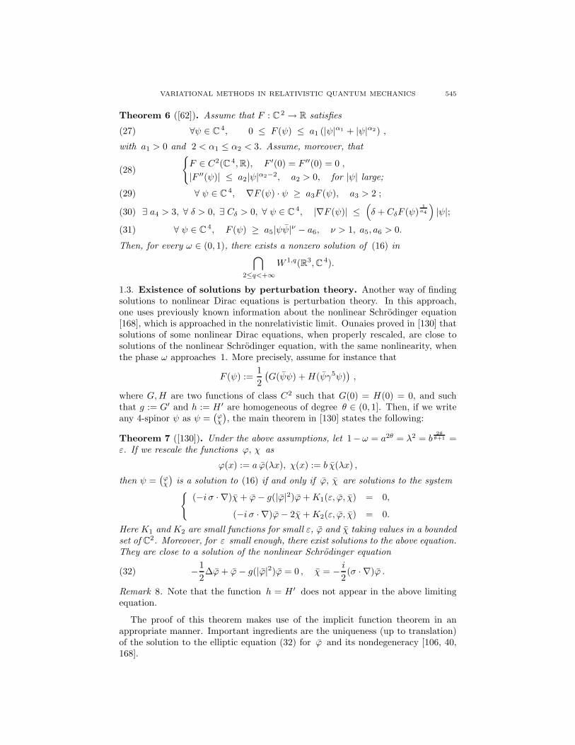
Theorem 6 ([62]). Assume that F : C 2 → R satisfies
(27) ∀ψ ∈ C4, 0 ≤ F (ψ) ≤ a1 (|ψ|α1 + |ψ|α2) ,
with a1 > 0 and 2 < α1 ≤ α2 < 3. Assume, moreover, thatF ∈ C2(C 4, R), F ′(0) = F ′′(0) = 0 ,
|F ′′(ψ)| ≤ a2|ψ|α2−2, a2 > 0, for |ψ| large;(28)
∀ ψ ∈ C4, ∇F (ψ) · ψ ≥ a3F (ψ), a3 > 2 ;(29)
∃ a4 > 3, ∀ δ > 0, ∃ Cδ > 0, ∀ ψ ∈ C4, |∇F (ψ)| ≤
(δ + CδF (ψ)
1a4
)|ψ|;(30)
∀ ψ ∈ C4, F (ψ) ≥ a5|ψψ|ν − a6, ν > 1, a5, a6 > 0.(31)
Then, for every ω ∈ (0, 1), there exists a nonzero solution of (16) in⋂2≤q<+∞
W 1,q(R3, C 4).
1.3. Existence of solutions by perturbation theory. Another way of findingsolutions to nonlinear Dirac equations is perturbation theory. In this approach,one uses previously known information about the nonlinear Schrodinger equation[168], which is approached in the nonrelativistic limit. Ounaies proved in [130] thatsolutions of some nonlinear Dirac equations, when properly rescaled, are close tosolutions of the nonlinear Schrodinger equation, with the same nonlinearity, whenthe phase ω approaches 1. More precisely, assume for instance that
F (ψ) :=12(G(ψψ) + H(ψγ5ψ)
),
where G, H are two functions of class C2 such that G(0) = H(0) = 0, and suchthat g := G′ and h := H ′ are homogeneous of degree θ ∈ (0, 1]. Then, if we writeany 4-spinor ψ as ψ =
(ϕχ
), the main theorem in [130] states the following:
Theorem 7 ([130]). Under the above assumptions, let 1−ω = a2θ = λ2 = b2θ
θ+1 =ε. If we rescale the functions ϕ, χ as
ϕ(x) := a ϕ(λx), χ(x) := b χ(λx) ,
then ψ =(ϕχ
)is a solution to (16) if and only if ϕ, χ are solutions to the system
(−i σ · ∇)χ + ϕ − g(|ϕ|2)ϕ + K1(ε, ϕ, χ) = 0,
(−i σ · ∇)ϕ − 2χ + K2(ε, ϕ, χ) = 0.
Here K1 and K2 are small functions for small ε, ϕ and χ taking values in a boundedset of C
2. Moreover, for ε small enough, there exist solutions to the above equation.They are close to a solution of the nonlinear Schrodinger equation
(32) −12∆ϕ + ϕ − g(|ϕ|2)ϕ = 0 , χ = − i
2(σ · ∇)ϕ .
Remark 8. Note that the function h = H ′ does not appear in the above limitingequation.
The proof of this theorem makes use of the implicit function theorem in anappropriate manner. Important ingredients are the uniqueness (up to translation)of the solution to the elliptic equation (32) for ϕ and its nondegeneracy [106, 40,168].

546 MARIA J. ESTEBAN, MATHIEU LEWIN, AND ERIC SERE
1.4. Nonlinear Dirac equations in the Schwarzschild metric. All of theabove models correspond to the Dirac equation written in the Minkowski metric,that is, in flat space. But space-time geometry plays an important role when onewants to take relativistic effects into account. For instance, when considering theSchwarzschild metric outside a massive star, the nonlinear Dirac equation appearsto be different.
In [9] A. Bachelot-Motet studied this problem numerically in the case of thesymmetric solutions as above. One has to study a system of O.D.E’s similar to (21)but with r-dependent coefficients instead of constant ones. More precisely, in theansatz (20) and for the case F (s) = λ|s|2 , system (21) becomes
(33)fu′ + u
r (f + f1/2) = v[λ(v2 − u2) − (f1/2 − ω)
],
fv′ + vr (f − f1/2) = u
[λ(v2 − u2) − (f1/2 + ω)
],
where f(r) = 1 − 1r .
Notice that this problem is not to be considered in the whole space: since thephysical situation corresponds to the outside of a massive star, the natural domainis the complement of a ball, or in radial coordinates, the interval r > r0 , for somer0 > 0 . In this case, the usual “MIT-bag” boundary condition reads
u(r0) = −v(r0) .
The very interesting numerical results obtained by Bachelot-Motet suggestedconditions for some existence and multiplicity results for (33) that were later rig-orously proved by Paturel in [131]. Note that in [131] the solutions are found ascritical points of a reduced energy functional by a mountain-pass argument, whileas we see below, we use a linking method to produce our solutions.
1.5. Solutions of the Maxwell-Dirac equations. The nonlinear terms appear-ing in all the above models are local, that is, they are functions of the spinor fieldΨ. But in some cases, one has to introduce nonlocal terms, for instance, such aswhen considering the interaction of the Dirac field with a self-generated field. Inthis case the equations become integro-differential.
Our first example is the Maxwell-Dirac system of classical field equations, de-scribing the interaction of a particle with its self-generated electromagnetic field.In order to write the equations in relativistically covariant form, we introduce theusual four-dimensional notations: let be γ0 := β and γk := βαk. For any wavefunc-tion Ψ(x0, x) : R × R3 → C4 (note that x0 plays the role of the time t), we denoteΨ := βΨ. In the Lorentz gauge the Maxwell-Dirac equations can be written as
(34)
(iγµ∂µ−γµAµ − 1)Ψ = 0 in R × R3,∂µAµ = 0, 4π ∂µ∂µ Aν = (Ψ, γνΨ) in R × R3.
Notice that we have used Einstein’s convention for the summation over µ. We alsointroduce the electromagnetic current Jν := (Ψ, γνΨ).
Finite energy stationary solutions of classical nonlinear wave equations have beensometimes used to describe extended particles. Of course the electromagnetic fieldshould in principle be quantized like in Quantum Electrodynamics. In the Maxwell-Dirac model, the field is not quantized but it is believed that interesting qualitativeresults can be obtained by using classical fields (see, e.g. [79, Chapter 7]).

VARIATIONAL METHODS IN RELATIVISTIC QUANTUM MECHANICS 547
Another example of a self-interaction is the Klein-Gordon-Dirac system whicharises in the so-called Yukawa model (see, e.g. [20]). It can be written as
(35)
(iγµ∂µ − χ − 1)Ψ = 0 in R × R3,∂µ∂µχ + M2χ = 1
4π (Ψ, Ψ) in R × R3 .
Other related models, which we will not discuss, include the Einstein-Dirac-Maxwellequations, which have been investigated by F. Finster, J. Smoller and S.-T. Yau [71],[72]. Systems (34) and (35) above have been extensively studied and many resultsare available concerning the Cauchy problem (we refer to [61] and [79, chapter 7]for detailed references).
A stationary solution of the Maxwell-Dirac system (34) is a particular solution(Ψ, A) : R × R4 → C4 × R4 of the form
(36)
Ψ(x0, x) = e−iωx0ψ(x) with ψ : R3 → C
4,
Aµ(x0, x) = Jµ ∗ 1|x| =
∫R3
dy|x−y| Jµ(y).
The existence of such stationary solutions of (34) has been an open problem for along time (see, e.g. [79, p. 235]). Indeed, the interaction between the spinor andits own electromagnetic field makes equations (34) nonlinear.
Concerning stationary solutions of (34), let us mention the pioneering works ofFinkelstein et al [69] and Wakano [166]. The latter considered this system in theapproximation A0 ≡ 0, A1 = A2 = A3 ≡ 0, the so-called Dirac-Poisson system.This problem can be reduced to a system of three coupled differential equationsby using the spherical spinors (20). Wakano obtained numerical evidence for theexistence of stationary solutions of the Dirac-Poisson equation. Further work in thisdirection (see [138]) yielded the same kind of numerical results for some modifiedMaxwell-Dirac equations which include some nonlinear self-coupling.
In [120] Lisi found numerical solutions of the Dirac-Poisson and of the Maxwell-Dirac systems. The computation of the magnetic part of the field A for thesesolutions showed that Wakano’s approximation was reasonable, since the field com-ponents (A1, A2, A3) stay small compared with A0. See also [136, 137, 24] wherevarious kinds of stationary solutions are considered, like the so-called static solu-tions which have no current “flow”.
In the case −1 < ω < 0, Esteban, Georgiev and Sere [61] used variationaltechniques to prove the existence of stationary solutions of (34). Any solutionof (34) taking the form (36) corresponds (formally) to a critical point ψ of thefunctional
Iω(ψ) =∫
R3
12
(iαk∂kψ, ψ)− 12
(ψ, ψ)−ω
2|ψ|2− 1
4
∫∫R3×R3
Jµ(x) Jµ(y)|x−y| dx dy.
This remark was used in [61] to find a stationary solution of (34) in the appropriatespace of functions.
Theorem 9 ([61]). For any ω strictly between −1 and 0, there exists a nonzerocritical point ψω of Iω. This function ψω is smooth in x and exponentially decreasingat infinity. Finally, the fields Ψ(x0, x) = e−iωx0 ψω, Aµ(x0, x) = Jµ
ω ∗ 1|x| are
solutions of the Maxwell-Dirac system (34).
Later, using cylindrical coordinates, S. Abenda [1] extended the result above tothe case −1 < ω < 1. Indeed, in the class of cylindrically symmetric functions, theenergy functional has better properties which allow us to use the same variational

548 MARIA J. ESTEBAN, MATHIEU LEWIN, AND ERIC SERE
procedure as in the work of Esteban and Sere, but in the more general case ω ∈(−1, 1).
Many questions are still open about the existence of stationary solutions for (34).It is easy to see that they have all a negative “mass”. Wakano already observed thisphenomenon for the soliton-like solutions of the Dirac-Poisson system. However, itwas shown in [166] that a positive mass can be reached by taking into account thevacuum polarization effect.
For the case of the Klein-Gordon-Dirac equations, the situation is slightly simplerbecause they are compatible with the ansatz (20) introduced above. So, in this casethe authors of [61] did not only obtain existence of solutions, but also multiplicity:
Theorem 10 ([61]). For any ω strictly between −1 and 0, there exists infinitelymany solutions to the Klein-Gordon-Dirac system (35). These solutions are allsmooth and exponentially decreasing at infinity in x.
We finish this section by explaining the general ideas of the proof of Theorem 9.The proofs of Theorems 4, 5 and 6 basically follow the same lines and we will skipthem.
Sketch of the proof of Theorem 9. As already mentioned in the Introduction,the presence of the negative spectrum for the Dirac operator forbids the use of aminimization argument to construct critical points. Instead, the solution will be ob-tained by means of a min-max variational method based on complicated topologicalarguments. The kinds of methods used to treat problems with infinite negative andpositive spectrum have been used already under the name of linking. The linkingmethod was introduced by V. Benci and P. Rabinowitz in a compact context [17].The reasons that make the use of variational arguments nonstandard in our caseare: (1) the equations are translation invariant, which creates a lack of compact-ness; (2) the interaction term JµAµ is not positive definite. Note that as we havealready pointed out, in some cases one can perform a reduction procedure and ob-tain a reduced functional for which critical points can be found by a mountain-passargument [131].
First step: Estimates. By defining Aµ = Jµ ∗ 1|x| , one then deduces JµAµ =
J0A0 −∑3
k=1 JkAk and
L(ψ) :=∫∫
R3×R3
Jµ(x) Jµ(y)|x−y| dx dy =
∫R3
JµAµ dx .
Let us also introduce the functional
(2.2) Q(ψ) =∫∫
R3×R3
(ψ, ψ)(x) (ψ, ψ)(y)|x−y| dx dy .
It is easy to prove that Q is nonnegative, continuous and convex on H=H1/2(R3, C4),and vanishes only when (ψ, ψ)(x) = 0 a.e. in R
3 .Let us state a lemma giving some properties of the quadratic forms in Iω.
Lemma 11. For any ψ ∈ H, the following inequalities hold:(i) JµAµ(x) ≥ 0 , a.e. in R3,(ii)
∫R3 JµAµ ≥ Q(ψ),
(iii) A0 ≥(∑3
k=1 |Ak|2)1/2
,
VARIATIONAL METHODS IN RELATIVISTIC QUANTUM MECHANICS 549
(iv) |γµAµψ| ≤ C√
A0√
AµJµ a.e. in R3.
Remark 12. Note that when the function ψ is cylindrically symmetric, the func-tional L defined above is not only nonnegative, but it actually controls from below‖ψ‖4
H(see Lemma 1 in [1]). This is the reason why Abenda has been able to treat
the case ω ∈ (−1, 1), extending Theorem 9.
Another important piece of information is given by
Lemma 13. Let µ > 0. There is a nonzero function e+ : (0;∞) → H+1 = Λ+
1 H
such that, if Λ+ψ = e+(µ), then12
∫R3
(ψ, D1ψ) − 14Q(ψ) ≤ µ
2‖ψ‖2
L2 .
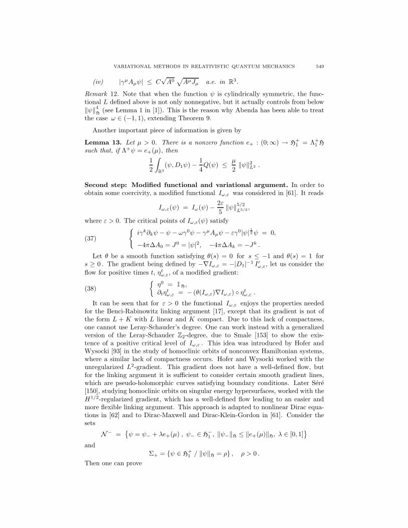
Second step: Modified functional and variational argument. In order toobtain some coercivity, a modified functional Iω,ε was considered in [61]. It reads
Iω,ε(ψ) = Iω(ψ) − 2ε
5‖ψ‖5/2
L5/2 ,
where ε > 0. The critical points of Iω,ε(ψ) satisfy
(37)
iγk∂kψ − ψ − ωγ0ψ − γµAµψ − εγ0|ψ| 12 ψ = 0,
−4π∆A0 = J0 = |ψ|2, −4π∆Ak = −Jk .
Let θ be a smooth function satisfying θ(s) = 0 for s ≤ −1 and θ(s) = 1 fors ≥ 0 . The gradient being defined by −∇Iω,ε = −|D1|−1 I ′ω,ε, let us consider theflow for positive times t, ηt
ω,ε, of a modified gradient:
(38)
η0 = H,∂tη
tω,ε = − (θ(Iω,ε)∇Iω,ε) ηt
ω,ε .
It can be seen that for ε > 0 the functional Iω,ε enjoys the properties neededfor the Benci-Rabinowitz linking argument [17], except that its gradient is not ofthe form L + K with L linear and K compact. Due to this lack of compactness,one cannot use Leray-Schauder’s degree. One can work instead with a generalizedversion of the Leray-Schauder Z2-degree, due to Smale [153] to show the exis-tence of a positive critical level of Iω,ε . This idea was introduced by Hofer andWysocki [93] in the study of homoclinic orbits of nonconvex Hamiltonian systems,where a similar lack of compactness occurs. Hofer and Wysocki worked with theunregularized L2-gradient. This gradient does not have a well-defined flow, butfor the linking argument it is sufficient to consider certain smooth gradient lines,which are pseudo-holomorphic curves satisfying boundary conditions. Later Sere[150], studying homoclinic orbits on singular energy hypersurfaces, worked with theH1/2-regularized gradient, which has a well-defined flow leading to an easier andmore flexible linking argument. This approach is adapted to nonlinear Dirac equa-tions in [62] and to Dirac-Maxwell and Dirac-Klein-Gordon in [61]. Consider thesets
N− =ψ = ψ− + λe+(µ) , ψ− ∈ H
−1 , ‖ψ−‖H ≤ ‖e+(µ)‖H, λ ∈ [0, 1]
and
Σ+ = ψ ∈ H+1 / ‖ψ‖H = ρ , ρ > 0 .
Then one can prove

550 MARIA J. ESTEBAN, MATHIEU LEWIN, AND ERIC SERE
Proposition 14. For any −1 < ω < −µ, ε > 0 and Σ+, N− constructed as above,there exists a positive constant cω, such that the set ηt
ω,ε(N−) ∩ Σ+ is nonempty,for all t ≥ 0. Moreover, the number
cω,ε = inft≥0
Iω,ε ηtω,ε(N−)
is strictly positive, it is a critical level for Iω,ε and cω,ε → cω > 0 as ε → 0.Additionally, for any ω, ε fixed, there is a sequence ϕn
ω,εn≥0 such that as n → +∞,
(39)
Iω,ε(ϕn
ω,ε) → cω,ε ,(1 + ‖ϕn
ω,ε‖)∇Iω,ε(ϕn
ω,ε) → 0 .
Remark 15. In [61] and [62], an easy regularization step is missing. Indeed, Smale’sdegree theory requires C2-regularity for the flow, which corresponds to C3-regularityfor the functional. In the case of the local nonlinear Dirac equation, such a regular-ity can be easily achieved by a small perturbation of the function F (ψ)+ε|ψ|α2−1ψ.Since all the estimates will be independent of the regularization parameter, the so-lutions of the nonregularized problem will be obtained by a limiting argument.
Note that the linking argument of [150], [62] and [61] has inspired later work (see[162, 157]), where an abstract linking theorem in a noncompact setting is given,valid first for C2- and then for C1-functionals.
Third step: Properties of the critical sequences. The concentration-com-pactness theory of P.-L. Lions [118] allows us to analyze the behavior of criticalsequences of Iω,ε as follows:
Proposition 16. Let ω ∈ (−1, 0) and ε ≥ 0 be fixed. Let (ψn) ⊂ H be a sequencein H such that
(40) 0 < infn
‖ψn‖H ≤ supn
‖ψn‖H < +∞,
and I ′ω,ε(ψn)→ 0 in H′ as n goes to +∞. Then we can find a finite integer p ≥ 1 , p
nonzero solutions ϕ1, . . . , ϕp of (37) in H and p sequences (xin) ⊂ R
3, i = 1, . . . , p,such that for i = j, |xi
n − xjn| →
n→+∞+∞ , and, up to extraction of a subsequence,
∥∥∥ψn −p∑
i=1
ϕi(· − xin)∥∥∥
H
→n→+∞
0 .
Obtaining estimates in H1/2(R3) for the sequence ϕnω,εn≥0 of Proposition 14
is quite easy because of the coercivity introduced by the perturbation term inε. Moreover, cω,ε being strictly positive, the sequence ϕn
ω,εn≥0 is also boundedfrom below away from 0. So, Proposition 16 applies to prove the existence of asolution to (37) for every ε > 0. Next, we want to pass to the limit when ε goesto 0. Note that we are doing so along a sequence of functions which are exactsolutions of the approximate problem (37). This part of the proof is done by firstproving the equivalent of the Pohozaev identity for equation (37), ε ≥ 0, and thenby introducing some special topologies in the spaces Lq which are related to thedecomposition of R3 as the union of unit cubes. Analyzing the solutions to (37)in those topologies, we find

VARIATIONAL METHODS IN RELATIVISTIC QUANTUM MECHANICS 551
Theorem 17. There is a constant κ > 0 such that if −1 < ω < 0 and 0 < ε ≤ 1,there is a function ψε ∈ H such that I ′ω,ε(ψε) = 0 and
κ ≤ Iω,ε(ψε) ≤ cω,ε .
Last step: Passing to the limit ε → 0. Eventually, we use Proposition 16to pass to the limit ε → 0. When obtaining the estimates (40) for the criticalsequences of Iω,ε , we observe that the lower estimate for the norm ||·||H is actuallyindependent of ε. Assume, by contradiction that the upper estimates do not holdfor the sequence (ψε). Then, we consider the normalized functions
ψε = ‖ψε‖−1H
ψε
and apply Proposition 16 to the sequence (ψε). Under the assumption that ||ψε||H→+ ∞, we use all the previous estimates to infer that for j = 1, . . . , p,
p∑j=1
∫R3
ϕjϕj + ω|ϕ|2 dx = 0 , Q(ϕj) = 0.
But the latter implies that for every j, ϕjϕj = 0 a.e., and so, from the right-handside identity we obtain that ϕj = 0 a.e. for all j. This contradicts Theorem 17.
1.6. Nonlinear Dirac evolution problems. The results that we have mentionedso far are concerned with the existence of stationary solutions of various nonlinearDirac evolution equations. These particular solutions are global and do not changetheir shape with time. The study of the nonlinear Dirac evolution problem,
(41)
i∂tΨ − D1Ψ + G(Ψ) = 0,Ψ(0) = Ψ0,
is also interesting in itself and, even if this is not the aim of the present paper, letus mention some references.
For the case of local nonlinearities such as the ones considered in this section, sev-eral works have proved well-posedness for small initial data in well-chosen Sobolevspaces. For nonlinearities containing only powers of Ψ of order p ≥ 4, Reed provedin [139] the global well-posedness for small initial data in Hs , s > 3. A decayestimate at infinity was also obtained in this paper. Later, Dias and Figueira [43]improved this result to include powers of order p = 3 and for s > 2. Najman [127]took the necessary regularity of the initial data down to H2. In [60] Escobedoand Vega proved an “optimal result” which states that for the physically relevantnonlinearities of order p ≥ 3 of the type
(42) G(Ψ) := λ
(ΨΨ)p−12 βΨ + b(Ψ, γ5Ψ)
p−12 γ5Ψ
,
there is local well-posedness of the evolution equation in Hs, for s > 32 −
1p−1 , when
p is an odd integer, while s has to be in the interval ( 32 − 1
p−1 , p−12 ) otherwise.
Moreover, if p > 3, then the problem is globally well-posed for small initial datain Hs(p), with s(p) = 3
2 − 1p−1 . For a more recent result, see for instance a paper
of Machihara, Nakanishi and Ozawa [121], in which the existence of small globalsolutions is proved in Hs for s > 1, and the nonrelativistic limit is also considered.
An interesting question to ask is about the (linear or nonlinear) stability proper-ties of the stationary solutions with respect to the flow generated by the evolutionequation. At present this seems to be a widely open problem (see [138] and [155]
552 MARIA J. ESTEBAN, MATHIEU LEWIN, AND ERIC SERE
for a discussion). Recently, Boussaid [21] has obtained the first stability results, forsmall stationary solutions of nonlinear Dirac equations with exterior potential.
Concerning the Cauchy problem for the Maxwell-Dirac equations, the first resultabout the local existence and uniqueness of solutions was obtained by L. Gross in[82]. Later developments were made by Chadam [34] and Chadam and Glassey[35] in 1 + 1 and 2 + 1 space-time dimensions and in 3 + 1 dimensions when themagnetic field is 0. In [38] Choquet-Bruhat studied the case of spinor fields ofzero mass and Maxwell-Dirac equations in the Minskowski space were studied byFlato, Simon and Taflin in [73]. In [76] Georgiev obtained a class of initial val-ues for which the Maxwell-Dirac equations have a global solution. This was per-formed by using a technique introduced by Klainerman (see [100, 101, 102]) toobtain L∞ a priori estimates via the Lorentz invariance of the equations and ageneralized version of the energy inequalities. The same method was used by Bach-elot [8] to obtain a similar result for the Klein-Gordon-Dirac equation. Finally,more recent efforts have been directed toward proving existence of solutions for thetime-dependent Klein-Gordon-Dirac and Maxwell-Dirac equations in the energyspace, namely C(−T, T ; H1/2 × H1). The existence and uniqueness of solutionsto the Maxwell-Dirac system in the energy space has been proved by Masmoudiand Nakanishi in [122, 123], improving Bournaveas’ result in [22], where the spaceconsidered was C(−T, T ; H1/2+ε × H1+ε).
Note that as mentioned above, the stationary states of the form (36) are particu-lar solutions of the Maxwell-Dirac equations. Physically they correspond to boundstates of the electron.
2. Linear Dirac equations for an electron in an external field
When looking for stationary states describing the dynamics of an electron movingin an external field generated by an electrostatic potential V , one is led to study theeigenvalues and eigenfunctions of the operator Dc +V . If the electron has to enjoysome stability, the eigenvalues should also be away from the essential spectrum. Inthe case of not very strong potentials V , the essential spectrum of Dc + V is thesame as that of Dc , that is, the set (−∞,−c2]∪ [c2, +∞). So the eigenvalues thatare of interest to us are those lying in the gap of the essential spectrum, i.e. inthe interval (−c2, c2). More precisely, in general a state describing an electron isalways assumed to correspond to a positive eigenvalue. It is therefore important tobe able to determine whether there are positive eigenvalues or not, and what is thebehaviour of the ‘first’ eigenvalue when V varies (whether it crosses 0 or dives intothe lower negative essential spectrum for instance). Note that one expects that for areasonable potential there are no eigenvalues embedded in the essential spectrum.Very general conditions on V that ensure nonexistence of embedded eigenvalueshave been given by [18, 19]. Finally note that in this section c is kept variable.
Formally, the eigenvalues of the operator Dc + V are critical values of theRayleigh quotient
(43) QV (ψ) :=((Dc + V )ψ, ψ)
(ψ, ψ)in the domain of Dc +V . Of course, one cannot use a minimizing argument to findsuch critical points since, due to the negative continuous spectrum of the free Diracoperator, QV is not bounded below. Many works have been devoted to findingnonminimization variational problems yielding the eigenvalues of Dc + V in the
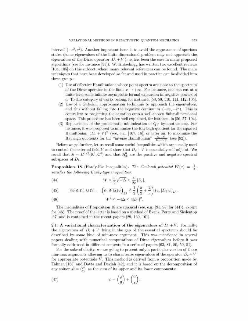
VARIATIONAL METHODS IN RELATIVISTIC QUANTUM MECHANICS 553
interval (−c2, c2). Another important issue is to avoid the appearance of spuriousstates (some eigenvalues of the finite-dimensional problem may not approach theeigenvalues of the Dirac operator Dc + V ), as has been the case in many proposedalgorithms (see for instance [55]). W. Kutzelnigg has written two excellent reviews[104, 105] on this subject, where many relevant references can be found. The maintechniques that have been developed so far and used in practice can be divided intothree groups:
(1) Use of effective Hamiltonians whose point spectra are close to the spectrumof the Dirac operator in the limit c → +∞. For instance, one can cut at afinite level some infinite asymptotic formal expansion in negative powers ofc. To this category of works belong, for instance, [58, 59, 110, 111, 112, 105].
(2) Use of a Galerkin approximation technique to approach the eigenvalues,and this without falling into the negative continuum (−∞,−c2). This isequivalent to projecting the equation onto a well-chosen finite-dimensionalspace. This procedure has been well explained, for instance, in [56, 57, 104].
(3) Replacement of the problematic minimization of QV by another one. Forinstance, it was proposed to minimize the Rayleigh quotient for the squaredHamiltonian (Dc + V )2 (see, e.g. [167, 16]) or later on, to maximize theRayleigh quotients for the “inverse Hamiltonian” Dc+V
|Dc+V |2 (see [92]).
Before we go further, let us recall some useful inequalities which are usually usedto control the external field V and show that Dc + V is essentially self-adjoint. Werecall that H = H1/2(R3, C4) and that H0
± are the positive and negative spectralsubspaces of D1.
Proposition 18 (Hardy-like inequalities). The Coulomb potential W (x) = 1|x|
satisfies the following Hardy-type inequalities:
W ≤ π
2
√−∆ ≤ π
2c|Dc|,(44)
∀ψ ∈ H0+ ∪ H
0−,
(ψ, W (x)ψ
)L2
≤ 12
(π
2+
2π
)(ψ, |D1|ψ)L2 ,(45)
W 2 ≤ −4∆ ≤ 4|D1|2.(46)
The inequalities of Proposition 18 are classical (see, e.g. [91, 98] for (44)), exceptfor (45). The proof of the latter is based on a method of Evans, Perry and Siedentop[67] and is contained in the recent papers [29, 160, 161].
2.1. A variational characterization of the eigenvalues of Dc + V . Formally,the eigenvalues of Dc + V lying in the gap of the essential spectrum should bedescribed by some kind of min-max argument. This was mentioned in severalpapers dealing with numerical computations of Dirac eigenvalues before it wasformally addressed in different contexts in a series of papers [63, 81, 80, 50, 51].
For the sake of clarity, we are going to present only a particular version of thosemin-max arguments allowing us to characterize eigenvalues of the operator Dc +Vfor appropriate potentials V . This method is derived from a proposition made byTalman [158] and Datta and Deviah [42], and it is based on the decomposition ofany spinor ψ =
(ϕχ
)as the sum of its upper and its lower components:
(47) ψ =(
ϕ
0
)+(
0χ
).

554 MARIA J. ESTEBAN, MATHIEU LEWIN, AND ERIC SERE
This proposal consisted in saying that the first eigenvalue of Dc + V could beobtained by solving the min-max problem
(48) minϕ=0
maxχ
((Dc + V )ψ, ψ)(ψ, ψ)
.
The first rigorous result on this min-max principle was obtained by Griesemerand Siedentop [81], who proved that (48) yields indeed the first positive eigenvalueof Dc+V for potentials V which are in L∞ and are not too large. In [51], Dolbeault,Esteban and Sere proved that if V satisfies the assumptions
(49) V (x) −→|x|→+∞ 0 ,
(50) − ν
|x| − K1 ≤ V ≤ K2 = supx∈R3
V (x) ,
(51) K1, K2 ≥ 0, K1 + K2 − c2 <√
c4 − ν2 c2
with ν ∈ (0, c), K1, K2 ∈ R, then the first eigenvalue λ1(V ) of Dc + V in theinterval (−c2, c2) is given by the formula
(52) λ1(V ) = infϕ=0
supχ
(ψ, (Dc + V )ψ)(ψ, ψ)
, ψ =(
ϕ
χ
).
Actually, under the conditions (49)–(50)–(51), it can be seen that Dc + V has aninfinite sequence of eigenvalues λk(V )k≥1 converging to 1, and it was proved in[51] that each of them can be obtained by the min-max procedure:
Theorem 19 (Min-max characterization of the eigenvalues of Dc + V [51]). LetV be a scalar potential satisfying (49)–(50)–(51). Then, for all k ≥ 1, the k-theigenvalue λk(V ) of the operator Dc + V is given by the min-max formula
(53) λk(V ) = infY subspace of C∞
o (R3,C 2)dimY =k
supϕ∈Y \0
λT(V, ϕ) ,
where
(54) λT(V, ϕ) := supψ=(ϕ
χ)χ∈C∞
0 (R3,C 2)
((Dc + V )ψ, ψ)(ψ, ψ)
is the unique number in (K2 − c2, +∞) such that
(55) λT (V, ϕ)∫
R3|ϕ|2dx=
∫R3
( c2 |(σ · ∇)ϕ|2c2 − V + λT (V, ϕ)
+ (c2 + V )|ϕ|2)dx.
The above result is optimal for Coulomb potentials for which all the casesν ∈ (0, c) are included. But note that assumptions (50)–(51) can be replaced byweaker ones allowing us to treat potentials which have a finite number of isolatedsingularities, even of different signs. We describe some of these extensions at theend of this subsection.
Theorem 19 is a useful tool from a practical point of view in the sense that thefirst eigenvalue (case k = 1) of Dc +V can be obtained by a minimization procedureover the (bounded-below) nonlinear functional ϕ → λT (V, ϕ). Higher eigenvaluesare obtained by the usual Rayleigh-Ritz minimax principle on the same nonlinear

VARIATIONAL METHODS IN RELATIVISTIC QUANTUM MECHANICS 555
functional. As we shall see below, this has important consequences from a numericalpoint of view.
Theorem 19 is a direct consequence of an abstract theorem proved by Dolbeault,Esteban and Sere [51], providing variational characterizations for the eigenvaluesof self-adjoint operators in the gaps of their essential spectrum.
Theorem 20 (Min-max principle for eigenvalues of operators with gaps [51]). LetH be a Hilbert space and A : D(A) ⊂ H → H a self-adjoint operator. We denote byF(A) the form-domain of A. Let H+, H− be two orthogonal Hilbert subspaces ofH such that H = H+⊕H−, and let Λ± be the projectors associated with H±. Weassume the existence of a subspace of D(A), F , which is dense in D(A) and suchthat
(i) F+ = Λ+F and F− = Λ−F are two subspaces of F(A).(ii) a− = supx−∈F−\0
(x−,Ax−)‖x−‖2
H< +∞ .
Moreover, we define the sequence of min-max levels
(56) ck(A) = infV subspace of F+
dim V =k
supx∈(V ⊕F−)\0
(x, Ax)||x||2H
, k ≥ 1,
and assume that(iii) c1(A) > a− .
Then∀k ≥ 1, ck(A) = µk,
where, if b = inf (σess(A)∩ (a−, +∞)) ∈ (a−, +∞], µk denotes the k-th eigenvalueof A (counted with multiplicity) in the interval (a−, b) if it exists, or µk = b if thereis no k-th eigenvalue.
As a consequence, b = limk→∞ ck(A) = supk ck(A) > a− .
An important feature of this min-max principle is that the min-max levels do notdepend on the splitting H = H+⊕H− provided assumptions (i), (ii) and (iii) holdtrue. In practice, one can find many different splittings satisfying these assumptionsand choose the most convenient one for a given application.
In order to treat families of operators without checking the assumptions of theabove theorem for every case, there is a “continuous” version of Theorem 20 in [51]that we shall present now.
Let us start with a self-adjoint operator A0 : D(A0) ⊂ H → H, and denote byF(A0) the form-domain of A0. Now, for ν in an interval [0, ν), we define Aν =A0 + νW , where W is a bounded operator. The operator Aν is self-adjoint withD(Aν) = D(A0), F(Aν) = F(A0). Let H = H+⊕H− be an orthogonal splitting ofH and P+ , P− the associated projectors, as in Section 1. We assume the existenceof a subspace of D(A0), F , dense in D(A0) and such that
(j) F+ = P+F and F− = P−F are two subspaces of F(A0);(jj) there is a− ∈ R such that for all ν ∈ (0, ν),
aν := supx−∈F−\0
(x−, Aνx−)‖x−‖2
H
≤ a−.
For ν ∈ (0, ν), let bν := inf(σess(Aν) ∩ (aν , +∞)) , and for k ≥ 1, let µk,ν be thek-th eigenvalue of Aν in the interval (aν , bν), counted with multiplicity, if it exists.If it does not exist, we simply let µk,ν := bν . Our next assumption is
(jjj) there is a+ > a− such that for all ν ∈ (0, ν), µ1,ν ≥ a+.

556 MARIA J. ESTEBAN, MATHIEU LEWIN, AND ERIC SERE
Finally, we define the min-max levels
(57) ck,ν := infV subspace of F+
dim V =k
supx∈(V ⊕F−)\0
(x, Aνx)||x||2H
, k ≥ 1 ,
and assume that
(jv) c1,0 > a− .
Then, we have
Theorem 21 ([51]). Under conditions (j) to (jv), Aν satisfies assumptions (i)–(iii) of Theorem 20 for all ν ∈ [0, ν), and ck,ν = µk,ν ≥ a+, for all k ≥ 1.
Theorems 20 and 21 are very good tools in the study of the point spectrum ofDirac operators Dc +νV , where V is a potential that has singularities not strongerthan c/|x − x0| (0 < c < 1). Of course, Theorem 21 cannot be directly applied tothe case of unbounded potentials, but this can actually be done by first truncatingthe potential and then passing to the limit in the truncation parameter, as we didin the proof of Theorem 19.
Theorem 21 is an easy consequence of the proof of Theorem 20. In contrast, theproof of Theorem 20 is more involved. We now sketch its main steps.
Sketch of the proof of Theorem 20. For E > a and x+ ∈ F+, let us define
ϕE,x+ : F− → R
y− → ϕE,x+(y−) =((x+ + y−), A(x+ + y−)
)− E||x+ + y−||2H .
From assumptions (i)–(ii), N(y−) =√
(a + 1)||y−||2H − (y−, Ay−) is a norm on
F−. Let FN
− be the completion of F− for this norm. Since ||.||H ≤ N on F−, we
have FN
− ⊂ H−. For all x+ ∈ F+, there is an x ∈ F such that Λ+x = x+ . If weconsider the new variable z− = y− − Λ−x, we can define
ψE,x(z−) := ϕE,Λ+x(z− + Λ−x) = (A(x + z−), x + z−) − E(x + z−, x + z−) .
Since F is a subspace of D(A), ψE,x (hence ϕE,x+) is well defined and continuousfor N , uniformly on bounded sets. So, ϕE,x+ has a unique continuous extension
ϕE,x+on F
N
−, which is continuous for the extended norm N . It is well known (seee.g. [140]) that there is a unique self-adjoint operator B : D(B) ⊂ H− → H− such
that D(B) is a subspace of FN
−, and
∀x− ∈ D(B), N(x−)2 = (a + 1)||x−||2H + (x−, Bx−).
Now, ϕE,x+is of class C2 on F
N
− and
D2ϕE,x+(x−) · (y−, y−) = −2(y−, By−) − 2E||y−||2H
≤ −2 min(1, E) N(y−)2 .(58)
So ϕE,x+has a unique maximum, at the point y− = LE(x+). The Euler-Lagrange
equations associated to this maximization problem are
(59) Λ−Ax+ − (B + E)y− = 0 .

VARIATIONAL METHODS IN RELATIVISTIC QUANTUM MECHANICS 557
The arguments above allow us, for any E > a, to define a map
QE : F+ → R
x+ → QE(x+) = supx−∈F−
ϕE,x+(x−) = ϕE,x+
(LEx+)(60)
= (x+, (A − E)x+) +(Λ−Ax+, (B + E)−1Λ−Ax+
).
It is easy to see that QE is a quadratic form with domain F+ ⊂ H+ and it ismonotone nonincreasing in E > a.
We may also, for E > a given, define the norm nE(x+) = ||x+ + LEx+||H . Weconsider the completion X of F+ for the norm nE and denote by nE the extendednorm. Then, we define another norm on F+ by
NE(x+) =√
QE(x+) + (KE + 1)(nE(x+))2
with KE = max(0, E2(E−λ1)λ2
1) and consider the completion G of F+ for the
norm NE . Finally, we use the monotonicity of the map E → QE and classi-cal tools of spectral theory to prove that the k-th eigenvalue of A in the interval(0, inf (σess(A) ∩ (a, +∞))) is the unique Ek > a such that
(61) infV subspace of G
dim V =k
supx+∈V \0
QEk(x+)
(nEk(x+))2
= 0 .
Note that since the above min-max levels correspond to the eigenvalues of theoperator TE associated to the quadratic form QE , (61) is actually equivalent to
λk(TEk) = 0,
and the fact that this inequality defines a unique Ek relies on the monotonicity ofQE w.r.t. E.
In applying Theorem 20 to prove Theorems 19 and 21, various decompositionsH = H+⊕H− could be considered. One that gives excellent resultsis defined by
(62) ψ =(
ϕ
0
)+(
0χ
).
This decomposition yields optimal results about the point spectrum for some po-tentials V . There are cases for which this is not true anymore. For instance, thishappens when the potential V has “large” positive and negative parts, a case whichis not dealt with in the previous results.
Recently, Dolbeault, Esteban and Sere [53] have considered the case where apotential can give rise to two different types of eigenvalues, not only those ap-pearing in Theorems 19 and 21. More precisely, if V satisfies (49), assume thatit is continuous everywhere except at two finite sets of isolated points, x+
i ,x−
j , i = 1, . . . I, j = 1, . . . , J, where
(63)
limx→x+
i
V (x) = +∞ , limx→x+
i
V (x) |x − x+i | ≤ νi,
limx→x−
j
V (x) = −∞ , limx→x−
j
V (x) |x − x−j | ≥ −νj ,
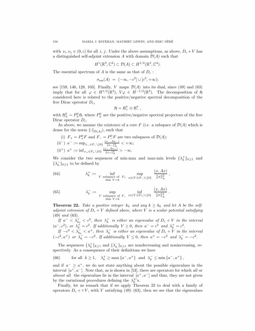
558 MARIA J. ESTEBAN, MATHIEU LEWIN, AND ERIC SERE
with νi, νj ∈ (0, c) for all i, j. Under the above assumptions, as above, Dc +V hasa distinguished self-adjoint extension A with domain D(A) such that
H1(R3, C4) ⊂ D(A) ⊂ H1/2(R3, C4).
The essential spectrum of A is the same as that of Dc :
σess(A) = (−∞,−c2] ∪ [c2, +∞);
see [159, 146, 128, 103]. Finally, V maps D(A) into its dual, since (49) and (63)imply that for all ϕ ∈ H1/2(R3), V ϕ ∈ H−1/2(R3). The decomposition of H
considered here is related to the positive/negative spectral decomposition of thefree Dirac operator Dc,
H = H0+ ⊕ H
0− ,
with H0± = P 0
±H, where P 0± are the positive/negative spectral projectors of the free
Dirac operator Dc.As above, we assume the existence of a core F (i.e. a subspace of D(A) which is
dense for the norm ‖·‖D(A)), such that
(i) F+ = P 0+F and F− = P 0
−F are two subspaces of D(A);(ii−) a− := supx−∈F−\0
(x−,Ax−)‖x−‖2
H
< +∞;
(ii+) a+ := infx+∈F+\0(x+,Ax+)‖x+‖2
H
> −∞.
We consider the two sequences of min-max and max-min levels λ+k k≥1 and
λ−k k≥1 to be defined by
(64) λ+k := inf
V subspace of F+dim V =k
supx∈(V ⊕F−)\0
(x, Ax)‖x‖2
H
,
(65) λ−k := sup
V subspace of F−dim V =k
infx∈(V ⊕F+)\0
(x, Ax)‖x‖2
H
.
Theorem 22. Take a positive integer k0 and any k ≥ k0 and let A be the self-adjoint extension of Dc + V defined above, where V is a scalar potential satisfying(49) and (63).
If a− < λ+k0
< c2, then λ+k is either an eigenvalue of Dc + V in the interval
(a−, c2), or λ+k = c2. If additionally V ≥ 0, then a− = c2 and λ+
k = c2.If −c2 < λ−
k0< a+, then λ−
k is either an eigenvalue of Dc + V in the interval(−c2, a+) or λ−
k = −c2. If additionally V ≤ 0, then a+ = −c2 and λ−k = −c2.
The sequences λ+k k≥1 and λ−
k k≥1 are nondecreasing and nonincreasing, re-spectively. As a consequence of their definitions we have
(66) for all k ≥ 1, λ+k ≥ max a−, a+ and λ−
k ≤ min a−, a+ ,
and if a− ≥ a+, we do not state anything about the possible eigenvalues in theinterval [a+, a−]. Note that, as is shown in [53], there are operators for which all oralmost all the eigenvalues lie in the interval [a+, a−] and thus, they are not givenby the variational procedures defining the λ±
k ’s.Finally, let us remark that if we apply Theorem 22 to deal with a family of
operators Dc + τ V , with V satisfying (49)–(63), then we see that the eigenvalues
VARIATIONAL METHODS IN RELATIVISTIC QUANTUM MECHANICS 559
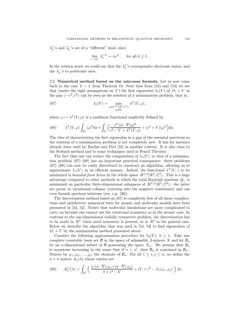
λ+k ’s and λ−
k ’s are of a “different” kind, since
limτ→0+
λτ,±k = ±c2 , for all k ≥ 1 .
In the written word, we could say that the λ+k ’s correspondto electronic states, and
the λ−k ’s to positronic ones.
2.2. Numerical method based on the min-max formula. Let us now comeback to the case k = 1 from Theorem 19. Note that from (52) and (54) we seethat (under the right assumptions on V ) the first eigenvalue λ1(V ) of Dc + V inthe gap (−c2, c2) can be seen as the solution of a minimization problem, that is,
(67) λ1(V ) = minϕ∈C∞(R3,C2)
ϕ=0
λT (V, ϕ) ,
where ϕ → λT (V, ϕ) is a nonlinear functional implicitly defined by
(68) λT (V, ϕ)∫
R3|ϕ|2dx=
∫R3
( c2 |(σ · ∇)ϕ|2c2 − V + λT (V, ϕ)
+ (c2 + V )|ϕ|2)dx.
The idea of characterizing the first eigenvalue in a gap of the essential spectrum asthe solution of a minimization problem is not completely new. It has for instancealready been used by Bayliss and Peel [16] in another context. It is also close tothe Fesbach method and to some techniques used in Pencil Theories.
The fact that one can reduce the computation of λ1(V ) to that of a minimiza-tion problem (67)–(68) has an important practical consequence: these problems(67)–(68) can now be easily discretized to construct an algorithm, allowing us toapproximate λ1(V ) in an efficient manner. Indeed, the functional λT (V, ·) to beminimized is bounded from below in the whole space H1/2(R3, C2) . This is a hugeadvantage compared to other methods in which the total Rayleigh quotient Qv isminimized on particular finite-dimensional subspaces of H1/2(R3, C4) : the latterare prone to variational collapse (entering into the negative continuum) and caneven furnish spurious solutions (see, e.g. [36]).
The discretization method based on (67) is completely free of all these complica-tions and satisfactory numerical tests for atomic and molecular models have beenpresented in [54, 52]. Notice that molecular simulations are more complicated tocarry on because one cannot use the rotational symmetry as in the atomic case. Incontrast to the one-dimensional radially symmetric problem, the discretization hasto be made in R2 when axial symmetry is present, or in R3 in the general case.Below we describe the algorithm that was used in [54, 52] to find eigenvalues ofDc + V by the minimization method presented above.
Consider the following approximation procedure for λk(V ), k ≥ 1. Take anycomplete countable basis set B in the space of admissible 2-spinors X and let Bn
be an n-dimensional subset of B generating the space Xn. We assume that Bn
is monotone increasing in the sense that if n < n′, then Bn is contained in Bn′ .Denote by ϕ1, ϕ2, . . . , ϕn the elements of Bn. For all 1 ≤ i, j ≤ n, we define then × n matrix An(λ) whose entries are
(69) Ai,jn (λ) =
∫R3
( (c (σ · ∇) ϕi, c (σ · ∇) ϕj)λ + c2 − V
+ (V + c2 − λ) (ϕi, ϕj))
dx.

560 MARIA J. ESTEBAN, MATHIEU LEWIN, AND ERIC SERE
The matrix An(λ) is self-adjoint and has therefore n real eigenvalues. For 1 ≤ k ≤n, we compute λk,n as the solution of the equation
(70) µk,n(λ) = 0 ,
where µk,n(λ) is the k-th eigenvalue of An(λ). Note that the uniqueness of such aλ comes from the monotonicity of the right-hand side of equation (69) with respectto λ. Moreover, since for a fixed λ
(71) µk,n(λ) µk(λ) as n → +∞ ,
we also have
(72) λk,n λk(V ) as n → +∞ .
The elements of the basis set used in [54] were Hermite functions. In [52] moreefficient numerical results have been obtained by means of B-spline functions. Theinterest of using well-localized basis set functions is the sparseness and the nicestructure of the corresponding discretized matrix An(λ). If the degree of the basisof B-splines increases, the number of filled diagonals will also increase. So, a goodbalance has to be found between the smoothness of elements of the approximatingbasis set and the speed of the corresponding numerical computations. In [52] thesimple choice of considering second-order spline functions on a variable length gridwas made. In the atomic case, when one-dimensional B-splines are used, very quickand accurate results can be obtained. In [52] numerical tests were provided for someaxially symmetric diatomic molecules.
In [109] we can find an algorithm which has some analogy with the algorithmdescribed above.
2.3. New Hardy-like inequalities. Another byproduct of the minimization char-acterization of the first eigenvalue of Dc + V given in (67) and of (55) is thefollowing: for all ϕ ∈ D(Dc + V ),
(73)∫
R3
(c2|(σ · ∇) ϕ|2
c2 − V + λ1(V )+ (c2 + V − λ1(V )) |ϕ|2
)dx ≥ 0.
In the particular case V = −ν/|x|, ν ∈ (0, c) , (73) means that for all ϕ ∈H1(R3, C2),(74)∫
R3
(c2|(σ · ∇) ϕ|2
c2 + ν/|x| +√
c4 − ν2 c2+ (c2 −
√c4 − ν2 c2) |ϕ|2
)dx ≥ ν
∫R3
|ϕ|2|x| dx.
By scaling, one finds that for all ϕ ∈ H1(R3, C2), and for all ν ∈ (0, 1),
(75)∫
R3
(|(σ · ∇) ϕ|2
1 + ν/|x| +√
1 − ν2+ (1 −
√1 − ν2) |ϕ|2
)dx ≥ ν
∫R3
|ϕ|2|x| dx ,
and, passing to the limit when ν tends to 1, we get:
(76)∫
R3
(|(σ · ∇) ϕ|21 + 1/|x| + |ϕ|2
)dx ≥
∫R3
|ϕ|2|x| dx .
This inequality is a Hardy-like inequality related to the Dirac operator. It is notinvariant under dilation, which corresponds to the fact that the Dirac operator Dc
VARIATIONAL METHODS IN RELATIVISTIC QUANTUM MECHANICS 561
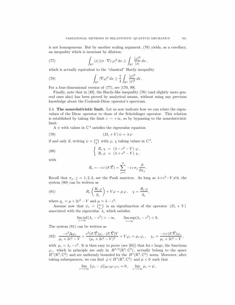
is not homogeneous. But by another scaling argument, (76) yields, as a corollary,an inequality which is invariant by dilation:
(77)∫
R3|x| |(σ · ∇) ϕ|2 dx ≥
∫R3
|ϕ|2|x| dx ,
which is actually equivalent to the “classical” Hardy inequality
(78)∫
R3|∇ϕ|2 dx ≥ 1
4
∫R3
|ϕ|2|x|2 dx .
For a four-dimensional version of (77), see [170, 99].Finally, note that in [49], the Hardy-like inequality (76) (and slightly more gen-
eral ones also) has been proved by analytical means, without using any previousknowledge about the Coulomb-Dirac operator’s spectrum.
2.4. The nonrelativistic limit. Let us now indicate how we can relate the eigen-values of the Dirac operator to those of the Schrodinger operator. This relationis established by taking the limit c → +∞, so by bypassing to the nonrelativisticlimit.
A ψ with values in C 4 satisfies the eigenvalue equation
(79) (Dc + V ) ψ = λ ψ
if and only if, writing ψ =(ϕχ
)with ϕ, χ taking values in C 2,
(80)
Rc χ = (λ − c2 − V ) ϕ ,Rc ϕ = (λ + c2 − V ) χ ,
with
Rc = −i c (σ.∇) =3∑
j=1
−i c σj∂
∂xj.
Recall that σj , j = 1, 2, 3, are the Pauli matrices. As long as λ+c2−V =0, thesystem (80) can be written as
(81) Rc
(Rc ϕ
gµ
)+ V ϕ = µ ϕ , χ =
Rc ϕ
gµ
,
where gµ
= µ + 2c2 − V and µ = λ − c2.Assume now that ψc =
(ϕc
χc
)is an eigenfunction of the operator (Dc + V )
associated with the eigenvalue λc which satisfies
lim infc→∞
(λc − c2) > −∞, lim supc→∞
(λc − c2) < 0.
The system (81) can be written as
(82)−c2∆ϕc
µc + 2c2 − V+
c2(σ.∇)ϕc · (σ.∇)V(µc + 2c2 − V )2
+ V ϕc = µc ϕc , χc =−i c (σ.∇)ϕc
µc + 2c2 − V,
with µc = λc − c2. It is then easy to prove (see [65]) that for c large, the functionsϕc , which in principle are only in H1/2(R3, C2) , actually belong to the spaceH1(R3, C2) and are uniformly bounded for the H1(R3, C2) norm. Moreover, aftertaking subsequences, we can find ϕ ∈ H1(R3, C2) and µ < 0 such that
limc→+∞
‖ϕc − ϕ‖H1(R3,C2) = 0 , limc→+∞
µc = µ ,

562 MARIA J. ESTEBAN, MATHIEU LEWIN, AND ERIC SERE
and
−∆ϕ
2+ V ϕ = µ ϕ .
Note that χc, the lower component of the eigenfunction ψc, converges to 0 in thenonrelativistic limit.
It can be proved that for all the potentials V considered in the theorems of thissection, all the eigenvalues in the gap (−c2, c2) satisfy the above conditions, andconverge, when shifted by the quantity −c2, to the associated eigenvalues of theSchrodinger operator −∆
2 perturbed by the same potential V .
2.5. Introduction of a constant external magnetic field. The previous resultswere devoted to the case of a scalar electrostatic field V . The Dirac operator fora hydrogenic atom interacting with a constant magnetic field in the x3-direction isgiven by
(83) DB := α ·[−i∇ +
B
2(−x2, x1, 0)
]+ β − ν
|x| ,
where ν = Zα > 0, Z being the nuclear charge number (we fix the speed of lightc = 1 in this subsection) and B is a constant.
The magnetic Dirac operator without the Coulomb potential ν/|x| has the essen-tial spectrum (−∞,−1]∪ [1,∞) and no eigenvalue in the gap (−1, 1) for any B ∈ R.The operator DB has the same essential spectrum and possibly some eigenvaluesin the gap. The ground state energy λ1(ν, B) is the smallest among these. As thefield gets large enough, one expects that the ground state energy of the Dirac op-erator decreases and eventually penetrates the lower continuum. The implicationof this for a second quantized model is that electron-positron pair creation comesinto the picture [129, 132]. The intuition comes from the Pauli equation, wherethe magnetic field tends to lower the energy because of the spin. It is thereforereasonable to define the critical field strength B(ν) as the supremum of the B’s forwhich λ1(ν, b) is in the gap (−1, 1) for all b < B. As a function of ν, λ1(ν, B) isnonincreasing, and as a result the function B(ν) is also nonincreasing. Estimateson this critical field as a function of the nuclear charge ν can be found in [48]. Theyhave been obtained by adapting to this case the variational arguments of Theorem19. One of the first results in this paper states that for all ν ∈ (0, 1),
(84)0.75ν2
≤ B(ν) ≤ min(
18πν2
[3ν2 − 2]2+, eC/ν2
).
As a corollary we see that as ν → 1 the critical field B(ν) stays strictly positive.This is somewhat remarkable, since in the case without magnetic field the groundstate energy λ1(ν, 0), as a function of ν, tends to 0 as ν → 1 but with an infiniteslope. Thus, one might expect very large variations of the eigenvalue at ν = 1 asthe magnetic field is turned on, in particular one might naively expect that theground state energy leaves the gap for small fields B. This is not the case.
Next, again by using the min-max characterization of λ1(ν, B),it is shown in [48]that for ν > 0 small enough and B not too large, λ1(ν, B) is asymptotically closeto the ground state energy of the Coulomb-Dirac magnetic operator inthe lowestrelativistic Landau level c0(ν, B). This constant is proved to be given by
(85) c0(ν, B) = inff∈C∞
0 (R,C)\0λB
0 (f) ,

VARIATIONAL METHODS IN RELATIVISTIC QUANTUM MECHANICS 563
where λB0 (f) is implicitly defined by
(86)
λB0 (f)
∫ +∞
−∞|f(z)|2 dz =
∫ +∞
−∞
(|f ′(z)|2
1 + λB0 (f) + ν aB
0 (z)+ (1 − ν aB
0 (z)) |f(z)|2)
dz,
and
aB0 (z) = B
∫ +∞
0
s e−Bs22
√s2 + z2
ds .
In [48] it is proved that for B not too small and ν small enough,
(87) c0(ν + ν3/2, B) ≤ λ1(ν, B) ≤ c0(ν, B),
and that since for ν small, ν3/2 ν,
c0(ν + ν3/2, B) ∼ c0(ν, B) ∼ λ1(ν, B) as ν → 0 .
The one-dimensional c0(ν, B) problem, while not trivial, is simpler to calculatethan the λ1(ν, B) problem. As a result, in the limit as ν → 0, this new theory yieldsthe first term in the asymptotics of the logarithm of the critical field. In particularwe have the following result,
limν→0
ν log(B(ν)) = π.
3. The Dirac-Fock equations for atoms and molecules
In the previous two sections we described some results concerning the solutionsof nonlinear or linear Dirac equations in R
3, which represent the state of one elec-tron only (or possibly many noninteracting electrons). We now want to presentthe Dirac-Fock (DF) model which allows us to describe the state of interactingelectrons, such as, for instance, N electrons in a molecule. The DF model is veryoften used in quantum chemistry computations and usually gives very good num-bers when the correlation between the electrons is negligible. It is the relativisticcounterpart of the better known nonrelativistic Hartree-Fock equations, which canindeed be seen as the nonrelativistic limit (c → ∞) of the Dirac-Fock model asexplained below. For this reason, we start by recalling briefly the Hartree-Fockmodel.
3.1. The (nonrelativistic) Hartree-Fock equations. The Hartree-Fock equa-tions are easily derived from the linear Schrodinger model in which one considersthe operator
(88) H :=N∑
i=1
(−∆xi
2+ V (xi)
)+
∑1≤i<j≤N
1|xi − xj |
,
whose associated quadratic form describes the energy of N interacting electrons inthe potential field V . Most often, V is the Coulomb electrostatic potential createdby a positive distribution of charge ν ≥ 0, of total charge Z:
V = −ν ∗ 1|x| ,
∫R3
ν = Z.
In the case of M pointwise nuclei of charges z1, ..., zM and located at x1, ..., xM ,one takes ν =
∑Mm=1 zmδxm
and Z =∑M
m=1 zm. But extended nuclei can also beconsidered, in which case ν is assumed to be a smooth L1 nonnegative function.
564 MARIA J. ESTEBAN, MATHIEU LEWIN, AND ERIC SERE
Due to the Pauli principle, the operator H acts on∧N
i=1 L2(R3 × ±, C), thatis to say the space of L2 functions Ψ(x1, σ1..., xN , σN ) which are antisymmetricwith respect to the permutations of the (xi, σi)’s. When Z > N − 1, it is known[171, 172] that the spectrum of H has the form σ(H) = λi ∪ [Σ,∞) where λiis an increasing sequence of eigenvalues with finite multiplicity converging to thebottom of the essential spectrum Σ. We notice that the condition Z > N − 1 playsa special role even for the linear theory based on the operator (88), as one knows[165, 96] that only finitely many eigenvalues exist below Σ when N ≥ Z + 1, andthat there is no eigenvalue below Σ when N Z [144, 151, 152, 115]. In thefollowing, we shall always assume that Z > N − 1.
In the Hartree-Fock approximation, one computes an approximation of the firsteigenvalue λ1 of H by restricting the quadratic form Ψ → 〈Ψ, HΨ〉 to the class ofthe functions Ψ which are a simple (Slater) determinant:
(89) Ψ = ϕ1 ∧ · · · ∧ ϕN ,
where (ϕ1, ..., ϕN ) is an orthonormal system of L2(R3 × ±, C) = L2(R3, C2),∫R3(ϕi, ϕj)C2 = δij . Denoting ϕi =
(ϕ+
i
ϕ−i
), (89) means more precisely
Ψ(x1, σ1, ..., xN , σN ) =1√N !
det(ϕσj
i (xj)).
Since the set of all the Ψ’s having the form (89) is not a vector subspace of∧Ni=1 L2(R3 × ±, C), one then obtains an energy functional which is nonlinear
in terms of ϕ1, ..., ϕN . The associated Euler-Lagrange equations form a system ofN coupled nonlinear PDEs:
(90) HΦ ϕk = λkϕk, k = 1, ..., N,
where HΦ is the so-called mean-field operator seen by each of the N electrons
(91) HΦ = −∆2
+ (ρΦ − ν) ∗ 1| · | −
γΦ(x, y)|x − y| ,
with ρΦ being the (scalar) electronic density and γΦ the so-called density matrix ofthe N electrons (this is a 2 × 2 matrix for any (x, y) ∈ R3 × R3):
(92) ρΦ :=N∑
i=1
|ϕi|2 and γΦ(x, y) :=N∑
i=1
ϕi(x) ⊗ ϕi(y)∗.
We notice that (91) means
(HΦ ψ)(x) = −∆ψ(x)2
+(
(ρΦ − ν) ∗ 1| · |
)(x)ψ(x) −
∫γΦ(x, y)ψ(y)
|x − y| dy
for any ψ ∈ H2(R3, C2). The existence of solutions to (90) when∫
R3 ν = Z > N −1has been proved first by Lieb and Simon [117] by a minimization method, and thenby Lions [119] by general min-max arguments. See also [108] for a recent survey.
3.2. Existence of solutions to the Dirac-Fock equations. The relativisticDirac-Fock equations were first introduced by Swirles in [156]. They take the sameform as the Hartree-Fock equations (90), with −∆/2 replaced by the Dirac opera-tor Dc. They are of course posed for functions taking values in C
4 instead of C2.
Note however that when −∆/2 is replaced by Dc in the formula of the N -bodyHamiltonian (88), one obtains an operator whose spectrum is the whole line R as

VARIATIONAL METHODS IN RELATIVISTIC QUANTUM MECHANICS 565
soon as N ≥ 2. To our knowledge, it is not known whether there exist or not eigen-values which are embedded in the essential spectrum. In any case, the relativisticN -body problem is not well-posed. This somehow restricts the physical interpre-tation of the Dirac-Fock model, compared to its nonrelativistic counterpart. Werefer to the next section in which a better model deduced from Quantum Electrody-namics is presented. Despite this issue, the Dirac-Fock equations have been widelyused in computational atomic physics and Quantum Chemistry to study atoms andmolecules involving heavy nuclei, and they seem to provide very good results whenthe correlation between the electrons is negligible.
In the case of N electrons, the Dirac-Fock equations read
(93) Dc,Φ ϕk
= εkϕk, k = 1, ..., N,
where Φ = (ϕ1, . . . , ϕN ) satisfies∫
R3(ϕi(x), ϕj(x)) dx = δij , i.e.
(94) Gram(Φ) = ,
and
Dc,Φ = Dc + (ρΦ − ν) ∗ 1|x| −
γΦ(x, y)|x − y| ,(95)
γΦ(x, y) =N∑
=1
ϕ(x) ⊗ ϕ
(y)∗, ρΦ(x) = trC4(γΦ(x, x)) =
N∑=1
|ϕ(x)|2.(96)
Notice that γΦ(x, y) is a 4× 4 complex matrix, and that the operator whose kernelis γΦ(x, y), is nothing but the orthogonal projector onto the space spanned byϕ1, ..., ϕN . We also denote it by γΦ.
Indeed, like for the Hartree-Fock case, equations (93) are the Euler-Lagrangeequations of the Dirac-Fock functional
(97) Eν,cDF(Φ) =
N∑=1
(ϕ
, Dcϕ
)L2
−N∑
=1
(ϕ
,
(ν ∗ 1
|x|
)ϕ
)L2
+12
∫∫R3×R3
ρΦ(x)ρΦ(y) − tr(γΦ(x, y)γΦ(y, x)
)|x − y| dx dy
on the manifold
M :=
Φ = (ϕ1, ..., ϕN ) ∈ H1/2(R3, C4)N , Gram(Φ) =
.
It will be important to notice that the functional Eν,cDF only depends on the projector
γΦ defined in (96):
(98) Eν,cDF(Φ) = “tr ((Dc + V )γΦ) ” +
12
∫∫R3×R3
ρΦ(x)ρΦ(y) − |γΦ(x, y)|2|x − y| dx dy ,
where by “tr ((Dc + V )γΦ)” we denote∑N
i=1((Dc + V )ϕi, ϕi). Note that this ex-pression is really a trace if the ϕi’s are in H1(R3, C4).
As a matter of fact, the Euler-Lagrange equations of Eν,cDF on M only depend on
the space spanned by (ϕ1, ..., ϕN ). This explains why, up to a rotation of the ϕi’s,one can always assume that the Lagrange multiplier matrix associated with theconstraint (94) is diagonal, with diagonal elements (ε1, ..., εN ) appearing in (93).

566 MARIA J. ESTEBAN, MATHIEU LEWIN, AND ERIC SERE
Finding solutions of (93) is then reduced to finding critical points of the func-tional Eν,c
DF on the manifold M. Once again, the unboundedness (from above andbelow) of the spectrum of the free Dirac operator makes the functional Eν,c
DF totallyindefinite. This together with the a priori lack of compactness of the problem posedin R3 and the fact that we have to work on a manifold M and not in the wholefunctional space, makes the variational problem difficult. A minimization proce-dure is once again impossible and another method has to be found. In [64], Estebanand Sere defined a penalized variational problem (see below for details) which canbe solved by first maximizing on some part of the spinor functions ϕi and thendefining a more standard min-max argument for the remaining functional, togetherwith Morse index considerations.
The theorem proved in [64] and improved later by Paturel in [131] states thefollowing:
Theorem 23 (Existence of solutions to the Dirac-Fock equations [64, 131]). Withthe above notation, assume that N and Z =
∫R3 ν are two positive integers satisfy-
ing max(Z, N) < 2cπ/2+2/π and N − 1 < Z. Then there exists an infinite sequence
(Φc,j)j≥0 of critical points of the Dirac-Fock functional Eν,c
DF on M. The functionsϕc,j
1 , . . . , ϕc,jN satisfy the normalization constraints (94) and they are strong solu-
tions, in H1/2(R3, C 4) ∩⋂
1≤q<3/2 W 1,q(R3, C 4), of the Dirac-Fock equations
Dc,Φc,j ϕc,jk
= εc,jk
ϕc,jk
, 1 ≤ k ≤ N,(99)
0 < εc,j1
≤ · · · ≤ εc,jN
< c2.(100)
Moreover,
0 < Eν,cDF(Φc,j) < Nc2,(101)
limj→∞
Eν,cDF(Φc,j) = Nc2.(102)
Remark 24. In our units, taking into account the physical value of the speed oflight c, the above conditions become
N ≤ Z ≤ 124.
The proof of the above theorem is done by defining a sequence of min-maxprinciples providing critical points of increasing Morse index. We notice that thesolution Φc,0 obtained by Theorem 23 when j = 0 will play an important role,since for c large it will actually be interpreted as an “electronic ground state” (seebelow).
The condition Z, N < 2c/(2π+π/2) is not that unnatural. Already in the linearcase this condition is related to Hardy-like inequalities ensuring the existence of agap of the spectrum of Dc + V around 0; see (45). Notice however that in [64] thefollowing additional technical assumption was used:
(103) 3N − 1 <2c
π/2 + 2/π.
This assumption was removed by Paturel shortly afterwards in [131]. He did soby studying a finite-dimensional reduction of the problem and then passing to thelimit, after having obtained the necessary bounds. This proof was done in the spiritof the Conley-Zehnder proof of Arnold’s conjecture [41]. The sketch of the proofthat we give below is that of [64] because the variational arguments are easier toexplain in that case.
VARIATIONAL METHODS IN RELATIVISTIC QUANTUM MECHANICS 567
Sketch of the proof of Theorem 23 when (103) holds. The first (and smallest)difficulty here is that ν∗ 1
|x| is not a compact perturbation of Dc when ν = Zδ0. Thiscreates some technical problems. They are easily solved, replacing the Coulombpotential 1
|x| by a regularized potential Vδ. The modified energy functional isdenoted now by Eν,c,η
DF . At the end of the proof, we shall be able to pass to thelimit η → 0.
The second difficulty is that the Morse index estimates can only give upperbounds on the multipliers εc,j
k in (99). But we also want to ensure that εc,jk > 0,
since these multipliers are interpreted as the energies of the different electrons. Toovercome this problem, we replace the constraint Gram (Φ) = by a penalizationterm πp(Φ), subtracted from the energy functional:
(104) πp(Φ) = tr[(
Gram Φ)p (− Gram Φ
)−1].
In this way we obtain a new functional Fc,η,p = Eν,c,ηDF −πp , defined now on the set
of Φ’s satisfying0 < Gram Φ < .
Since in the basis in which
Gram Φ = Diag(σ1, . . . , σN ) , 0 < σ1 ≤ · · · ≤ σN < c2 ,
the matrix(Gram Φ
)p (− Gram Φ)−1
is also diagonal and equals
Diag(fp(σ1), . . . , fp(σN )) , with fp(x) :=xp
1 − x,
the corresponding Euler-Lagrange equations are then
Dc,Φc,j ϕc,jk = f ′
p(σc,jk ) ϕc,j
k .
The numbers εc,jk := f ′
p(σc,jk ) are now explicit functions of ϕc,j
k . Thus, fp being anincreasing function, we automatically get εc,j
k > 0.The third difficulty with DF, is that all critical points have an infinite Morse
index. This kind of problem is often encountered in the theory of Hamiltoniansystems and in certain elliptic PDEs. One way of dealing with it is to use a concavityproperty of the functional, to get rid of the “negative directions”, see e.g. [2, 27,28, 31]. This method was used in [64]. Doing so, we get a reduced functionalIc,η,p. A min-max argument gives us Palais-Smale sequences (Φc,η,p
n )n≥1 for Ic,η,p
with a Morse index “at most j” (up to an error which converges to 0 as n → ∞),thanks to [68, 77]. Moreover, adapting the arguments of [119], we prove that thecorresponding εc,j,η,p,n
k are bounded away from c2. Finally, the assumptions madeon Z, N guarantee that the εc,j,η,p,n
k are also bounded away from 0, uniformly onη, p and n. Then we pass to the limit (η, p, n) → (0,∞,∞), and get the desiredsolutions of DF, with 0 < εc,j
k < c2.The fact that we recover at the limit p → +∞ the constraint Gram Φ = is a
consequence of the a priori estimates
0 < ε < εc,j,η,pk = f ′
p(σc,j,η,pk ) ,
with ε independent of η, p. The properties of the function fp and the above in-equality imply that as p → +∞ , one necessarily has σc,j,η,p → 1, which of courseis equivalent to saying that in the limit there is no loss of charge:
∫R3 |ϕc,j
k |2 = 1.
568 MARIA J. ESTEBAN, MATHIEU LEWIN, AND ERIC SERE
The method that we have just described can be generalized. In [26] an abstractversion is provided with applications to nonlinear periodic Schrodinger models aris-ing in the physics of crystalline matter.
The concavity argument of [64] works only if (103) holds. In his theorem, Paturel[131] got rid of this assumption by making a finite-dimensional reduction first. Thisallowed him to deal with finite Morse indices again.
3.3. Nonrelativistic limit and definition of the Dirac-Fock “ground state”.As in the case of the linear Dirac equations of Section 3, it is interesting here to seewhat is the nonrelativistic limit of the Dirac-Fock equations. We shall recover inthe limit the Hartree-Fock equations (90) presented above, for the two-dimensionalupper component of the ϕi’s (recall that ϕ1, ..., ϕN are C4-valued functions), thelower component converging to zero. This was proved rigorously in [65]. Thisresult has been of importance to better understand the variational structure of theDirac-Fock problem and in particular to obtain a good definition of an electronicground-state energy, which is a priori not clear because of the unboundedness ofthe Dirac-Fock energy.
Theorem 25 (Nonrelativistic limit of the Dirac-Fock equations [65]). Let be N <Z+1. Consider a sequence of numbers cn → +∞ and a sequence (Φn)n of solutionsof (93), i.e. Φn = (ϕn
1 , ..., ϕnN ), each ϕn
k being in H1/2(R3, C4), with Gram Φn = and Dcn,Φnϕn
k = εnkϕn
k . Assume that the multipliers εnk , k = 1, . . . , N, satisfy
0 < ε < εn1 ≤ · · · ≤ εn
N < c2 − ε′, with ε, ε′ > 0 independent of n.
Then for n large enough, each ϕnk is in H1(R3, C4), and there exists a solution of
the Hartree-Fock equations (90), Φ = (ϕ1, · · · , ϕN ) ∈ H1(R3, C2)N , with negativemultipliers, λ1, ..., λN , such that, after extraction of a subsequence,
(105) limn→∞
(εnk − (cn)2) = λk,
ϕnk =
(ϕn
k
χnk
)−→n→+∞
(ϕk
0
)in H1(R3, C 2) × H1(R3, C 2),(106)
∥∥∥∥χnk +
i
2cn(σ · ∇)ϕn
k
∥∥∥∥L2(R3,C 2)
= O(1/(cn)3),(107)
for all k = 1, ..., N , and
(108) Eν,cn
DF (Φn) − Nc2n −→
n→+∞EHF(Φ).
The Hartree-Fock energy EHF appearing in (108) is the same as (97), but withDc replaced by −∆/2 and C
4 by C2. It can be proved [65] that the critical points
constructed in Theorem 23 all satisfy the assumptions of Theorem 25 for any fixedj. Therefore, all the Φc,j converge as c → ∞ to a state whose upper component is asolution of the Hartree-Fock equations, and whose lower component vanishes. Thisresult can even be made more precise in the case of one of the “first” solutions (i.e.corresponding to j = 0): the critical point Φc,0 does not converge to any solutionof the HF equations, but actually to a Hartree-Fock ground state, as stated in

VARIATIONAL METHODS IN RELATIVISTIC QUANTUM MECHANICS 569
Theorem 26 (Nonrelativistic limit of the Dirac-Fock “ground state” [65]). Assumethat N < Z + 1 and ν are fixed, and that cn → ∞. Then the critical point Φcn,0
constructed in Theorem 23 for j = 0 satisfies
limcn→∞
Eν,cDF(Φcn,0) − Nc2
n
= min
Φ∈H1(R3,C2)N
Gram Φ=EHF(Φ).
Up to a subsequence, (Φcn,0) converges as cn → ∞ to(
Φ00
), where Φ0 is a minimizer
of EHF. Furthermore, for cn large enough, the εcn,0k are the first positive eigenvalues
of Dcn,Φcn,0 :
(109) γΦcn,0 = χ[0,εcn,0N ]
(Dcn,Φcn,0
).
We notice that (109) means that the last level εcn,0N is necessarily totally filled.
In other words, similar to the Hartree-Fock case [7], “there are no unfilled shells inthe Dirac-Fock theory for c 1”.
σ(Dc,Φc,0
)Φc,0
Figure 1. For c 1, the Dirac-Fock “ground state” Φc,0 containsthe eigenfunctions associated with the N first positive eigenvaluesof the mean-field operator Dc,Φc,0 .
Although the Dirac-Fock functional Eν,cDF is not bounded below, Theorem 26
allows us to interpret the first min-max solution Φc,0 (any of them, since there isno uniqueness) as an electronic ground state, since it converges to a Hartree-Fockground state in the nonrelativistic limit. Actually, more has been proved in [65]:Φc,0 indeed minimizes the Dirac-Fock functional among all the Φ = (ϕ1, ..., ϕN ) suchthat each ϕi belongs to the positive spectral subspace of the mean-field operatorDc,Φ:
Theorem 27 (Variational interpretation of the Dirac-Fock “ground state” [65]).Assume that N < Z + 1 and ν are fixed, and that c is sufficiently large. Then Φc,0
is a solution of the following minimization problem:
(110) infEν,cDF(Φ) | Φ = (ϕ1, ..., ϕN ), Gram Φ = , χ(−∞,0) (Dc,Φ) Φ = 0
,
where χ(−∞,0)(Dc,Φ) denotes the negative spectral projector of the operator Dc,Φ,and
χ(−∞,0) (Dc,Φ) Φ = 0means
χ(−∞,0) (Dc,Φ) ϕk = 0for any k = 1, ..., N .
The interpretation of the theorem is the following: Although the Dirac-Fockenergy is unbounded from below, the critical points Φc,0 are, for c large enough,the minimizers of Eν,c
DF on the set of functions satisfying the nonlinear conditionχ(−∞,0) (Dc,Φ) Φ = 0. Calling these functions electronic, we obtain that for c large,Φc,0 is really an electronic ground state. In particular, it is also a minimizer of Eν,c
DF
among all the solutions of Dirac-Fock equations with positive Lagrange multipliers.
570 MARIA J. ESTEBAN, MATHIEU LEWIN, AND ERIC SERE
Remark 28. Recently, explicit bounds on c under which Theorem 27 is valid havebeen provided by Huber and Siedentop [94].
4. The mean-field approximation in Quantum Electrodynamics
In this last section, we want to present some progress that has been made recentlyconcerning models from Quantum Electrodynamics (QED) in which, instead oftrying to “avoid” the negative spectrum of Dc, the latter is reinterpreted as Dirac’svacuum and completely “incorporated” into the model. The somehow surprisingconsequence will be that, contrary to the previous sections, the energy functionalwill be bounded from below. The price to pay is that one has to deal with infinitelymany particles (many of them being “virtual”) instead of the finite number ofelectrons as previously.
As mentioned in the Introduction, Dirac interpreted the negative spectrum ofhis operator Dc as follows [45, 46, 47]. Since there exists no electron of negativekinetic energy, one has to find a way of avoiding the negative spectrum. This isdone by assuming that the negative spectrum energies are all occupied by virtualelectrons, one in each energy state, and that this (virtual) distribution of charge isnot felt by the real particles on account on its uniformity. Then, the real electronscan in general only have positive energies due to the Pauli principle which preventsthem from being in the same state as a virtual particle.
Mathematically, Dirac’s postulate is interpreted as follows: the states of the realfree electrons necessarily belong to the positive spectral subspace H0
+,c = P 0+,c H
defined in Proposition 1, and the vacuum (Dirac sea) is described by the infiniterank spectral projector P 0
−,c. Recall that in Hartree or Dirac-Fock theories, thedensity matrix γΦ of the N electron state Ψ = ϕ1∧· · ·∧ϕN is precisely the orthog-onal projector onto span(ϕ1, ..., ϕN ), see, e.g. formulas (89) and (92). Therefore,when one represents the Dirac sea by the projector P 0
−,c, one describes formally thevacuum as an infinite Slater determinant
(111) Ω0 = ϕ1 ∧ · · · ∧ ϕi ∧ · · · ,
where (ϕi)i≥1 is an orthonormal basis of H0−,c = P 0
−,c H. Dirac’s postulate is basedon the important invariance by translation of the projector P 0
−,c, which is used toneglect the physical influence of this “constant background”.
It was realized just after Dirac’s discovery that, for consistency of the theory,the vacuum should not be considered as a totally virtual physical object that doesnot interact with the real particles. Dirac himself [45, 46, 47] conjectured theexistence of surprising physical effects as a consequence of his theory, which werethen experimentally confirmed. First, the virtual electrons of the Dirac sea canfeel an external field and they will react to this field accordingly, i.e. the vacuumwill become polarized. This polarization is then felt by the real particles, and onetherefore is led to consider a coupled system “Dirac sea + real particles”. Fromthe experimental viewpoint, vacuum polarization plays a rather small role for thecalculation of the Lamb shift of hydrogen but it is important for high-Z atoms[126], and it is even a crucial physical effect for muonic atoms [75, 78]. Second, inthe presence of strong external fields, the vacuum could react so importantly thatan electron-positron pair can be spontaneously created [129, 141, 142, 143].
The mathematical difficulties of a model aiming at describing both the Diracsea and the real particles are important, for one has to deal at the same time

VARIATIONAL METHODS IN RELATIVISTIC QUANTUM MECHANICS 571
with infinitely many particles (the real ones and the virtual ones of the Diracsea). In the following, we present a Hartree-Fock (mean-field) type model for thisproblem that has been mathematically studied by Hainzl, Lewin, Sere and Solovej[83, 84, 85, 86]. The model under consideration is inspired by an important physicalarticle by Chaix and Iracane [36] in which the possibility that a bounded-belowenergy could be obtained by adding vacuum polarization was first proposed. Butthe equations of this so-called Bogoliubov-Dirac-Fock model were already knownin Quantum Electrodynamics (QED) [142]. For the sake of simplicity, we shall notexplain how the model is derived from the QED Hamiltonian, and we refer thereader to [83, 84, 85, 86] and the review [87]. In the version studied in these works,the electromagnetic field is not quantized (photons are not considered).
Let us now describe formally the mean-field approximation in QED, followingmainly [86, 87]. The state of our system will be represented by an infinite rankprojector P . This projector should be seen as the density matrix of an infiniteSlater determinant made of an orthonormal basis of the subspace PH, such as(111). The projector P describes not only Dirac’s vacuum but the whole systemconsisting of the infinitely many virtual particles of the vacuum, together withthe finitely many real particles (they could be electrons or positrons). Indeed, itis important to realize that in this model there is no a priori possible distinctionbetween the real and the virtual particles. For N electrons, this would correspondto a decomposition of the form P = Pvac + γ, where γ is an orthogonal projector ofrank N satisfying Pvacγ = γPvac = 0 (for N positrons, this becomes P = Pvac − γ).But there are infinitely many such decompositions for a given P and a given N : itwill only be for the final solution of our equation that this decomposition will bedone in a natural way.
For the sake of simplicity, we take c = 1 except at the very end of this section.We recall that in this case an additional parameter α = e2 appears, where e is thecharge of the electron. The energy in the state P of our system in the presence ofan external field V = −αν ∗ | · |−1 is then formally given [86] by
(112) EνQED(P ) := Eν(P − 1/2),
where Eν is the Dirac-Fock functional expressed in terms of the density matrix (see(98))
(113) Eν(Γ) := tr(D1Γ) − α
∫R3
(ν ∗ 1
| · |
)(x)ρΓ(x) dx
+α
2
∫∫R3×R3
ρΓ(x)ρΓ(y)|x − y| dx dy − α
2
∫∫R3×R3
|Γ(x, y)|2|x − y| dx dy.
The density of charge ν which creates the field V can for instance represent a systemof nuclei in a molecule. But in the following we shall not allow pointwise nuclei aswe did for the Dirac-Fock model, and ν will essentially be an L1
loc function. This isnot important as pointwise particles do not exist in nature.
The subtraction of half the identity in (112) is a kind of renormalization whichwas introduced by Heisenberg [89] and has been widely used by Schwinger (see[147, eq. (1.14)], [148, eq. (1.69)] and [149, eq. (2.3)]) as a necessity for a covariantformulation of QED. The importance of this renormalization will be clarified below.
Before we come to the problems of definition of the above energy (which arenumerous), let us mention briefly how Eν
QED is supposed to be used. There are
572 MARIA J. ESTEBAN, MATHIEU LEWIN, AND ERIC SERE
two possibilities. If one wants to find the state of the vacuum alone in the fieldV (no particle at all), then one has to minimize P → Eν(P − 1/2) on the wholeset of orthogonal projectors. When ν = 0, one should obtain the free vacuum,a translation-invariant projector which is supposed to be physically unimportant.When ν = 0, one should obtain the polarized vacuum in the presence of the fieldV . It can be seen formally that such a minimizer P should be a solution of thenonlinear equation
(114) P = χ(−∞,0)
(D1 + α(ρ[P−1/2] − ν) ∗ 1
| · | − α(P − 1/2)(x, y)
|x − y|
).
If one wants to describe a system containing N real particles (or more correctly oftotal charge −eN), then one has to minimize P → Eν(P−1/2) under the additionalconstraint tr(P − 1/2) = N . Usually this will provide us with a projector P whichdescribes adequately the state of a system of charge −eN interacting with Dirac’svacuum. It is formally a solution of the nonlinear equation
(115) P = χ(−∞,µ]
(D1 + α(ρ[P−1/2] − ν) ∗ 1
| · | − α(P − 1/2)(x, y)
|x − y|
),
µ being a Lagrange multiplier due to the charge constraint. If ν is not too strong,the mean-field operator
D := D1 + α(ρ[P−1/2] − ν) ∗ 1| · | − α
(P − 1/2)(x, y)|x − y|
will have exactly N eigenvalues in [0, µ] (counted with their multiplicity). Therefore,there will be a natural decomposition
P = χ(−∞,0) (D) + χ[0,µ] (D) = χ(−∞,0) (D) +N∑
=1
ϕi ⊗ ϕi,
where the ϕi’s are solutions of
(116) Dϕk = εk ϕk, εk > 0,
which is the natural decomposition between the real and the virtual particles men-tioned above. It will be shown below that equations (116) are very close to theDirac-Fock equations (93).
The goal is now to give a mathematical meaning to this program.First, one has to face an important difficulty: When P is an orthogonal projector
and H is infinite dimensional, then P −1/2 is never compact. Therefore, none of theterms of (113) makes sense. In [86], Hainzl, Lewin and Solovej tackled this problemin the following way: They considered a box CL := [−L/2, L/2)3 of volume L3 andreplaced the ambient space H by the space L2
per(CL) of L2 functions on CL withperiodic boundary conditions, with moreover a cut-off in Fourier space. Doing so,the problem becomes finite dimensional and everything makes perfect sense. Then,when no charge constraint is imposed, they took the thermodynamic limit L → ∞with the Fourier cut-off fixed and proved that the sequence of minimizers convergesto a limiting projector P satisfying equation (114). In this way, they could give ameaning to the minimization of the QED functional (112) and to equation (114).Moreover, they also obtained the so-called Bogoliubov-Dirac-Fock (BDF) energywhich attains its minimum at the limit state P . This energy has been studied byHainzl, Lewin and Sere in [83, 84, 85]. In the following, we describe all these resultsin more detail.

VARIATIONAL METHODS IN RELATIVISTIC QUANTUM MECHANICS 573
Notice that the Fourier cut-off will not be removed in this study. Indeed it iswell known that QED contains important divergences that are difficult to remove.Therefore H will be replaced by the functional space
HΛ :=f ∈ L2(R3, C4), supp(f) ⊂ B(0, Λ)
.
The ideas described in this section have recently been adapted [30] to a nonlinearmodel of solid state physics describing nonrelativistic electrons in a crystal with adefect.
4.1. Definition of the free vacuum. We start by explaining how the free vacuumwas constructed in [86], in the case ν = 0. This is done by defining the energy (113)for projectors P acting on the finite-dimensional space
HLΛ :=
f ∈ L2
per([−L/2, L/2)3, C4), supp(f) ⊂ B(0, Λ)
= spanexp(ik · x), k ∈ (2π/L)Z3 ∩ B(0, Λ)
.
To define the energy properly, it is necessary to periodize the Coulomb potentialas follows:
WL(x) =1L3
⎛⎜⎜⎝ ∑k∈(2π)Z3/L
k =0
4π
|k|2 eik·x + wL2
⎞⎟⎟⎠ ,
where w is some constant which is chosen such that min CLWL = 0 for any L. The
Dirac operator D1 is also easily defined on HLΛ: it is just the multiplication of the
Fourier coefficients by (D1(k))k∈2πZ3/L. Then, one introduces
(117) E0L(Γ) := trHL
Λ(D1Γ) + +
α
2
∫∫CL×CL
WL(x − y)ρΓ(x)ρΓ(y) dx dy
− α
2
∫∫CL×CL
WL(x − y)|Γ(x, y)|2dx dy ,
for any self-adjoint operator Γ acting on HLΛ. The kernel Γ(x, y) of Γ is easily
defined since HLΛ is finite dimensional. Its density ρΓ is then defined as ρΓ(x) :=
trC4(Γ(x, x)). A translation-invariant operator T acting on HLΛ is by definition a
multiplication operator in the Fourier domain. In this case, one has T (x, y) =f(x − y) for some f and therefore ρT is constant. The identity of HL
Λ, denoted byILΛ is an example of a translation-invariant operator.
The first result proved in [86] is the following:
Theorem 29 (QED mean-field minimizer in a box [86]). Assume that 0 ≤ α < 4/π,Λ > 0 and that L is large enough. Then the functional E0
L has a unique minimizerΓ0
L on the convex set
GLΛ :=
Γ ∈ L(HL
Λ), Γ∗ = Γ, −ILΛ/2 ≤ Γ ≤ IL
Λ/2
.
It is invariant by translation and satisfies ρΓ0L≡ 0. Moreover, it takes the form
Γ0L = P0
L − ILΛ/2, where P0
L is an orthogonal projector on HLΛ.
Notice that in the definition of the variational set GLΛ , we did not consider only
operators taking the form P−ILΛ/2 , where P is an orthogonal projector as suggested
by (112), but we indeed extended the energy functional to the convex hull of this

574 MARIA J. ESTEBAN, MATHIEU LEWIN, AND ERIC SERE
set. But, as usual in Hartree-Fock type theories [113], the global minimizer is alwaysan extremal point, i.e. a state taking the form P − IL
Λ/2.Of course, it can easily be shown that P0
L satisfies an equation similar to (114)with ν removed and 1/|x| replaced by WL. But we do not give the details since weare more interested in the limit of P0
L as L → ∞.To be able to state the thermodynamic limit correctly, one needs first to introduce
the translation-invariant projector P0− acting on HΛ, which will be the limit of the
sequence (P0L)L. The identity of HΛ is denoted by IΛ. We introduce
(118)
T (A) =1
(2π)3
∫B(0,Λ)
trC4 [D0(p)A(p)]dp− α
(2π)5
∫∫B(0,Λ)2
trC4 [A(p)A(q)]|p − q|2 dp dq
for any A belonging to the convex set
AΛ := A translation invariant on HΛ, A∗ = A, −IΛ/2 ≤ A ≤ IΛ/2 .
It will be shown in Theorem 31 below that T represents the energy per unit volumeof translation-invariant operators. For this reason, one now considers the minimiza-tion of T on AΛ. The following was proved in [86]:
Theorem 30 (Definition of the free vacuum [86]). Assume that 0 ≤ α < 4/π andΛ > 0. Then T possesses a unique global minimizer Γ0 on AΛ. It satisfies theself-consistent equation
(119)
⎧⎪⎨⎪⎩Γ0 = − sgn(D0)
2,
D0 = D1 − αΓ0(x, y)|x − y|
or, written in terms of the translation-invariant projector P0− = Γ0 + IΛ/2,
(120) P0− = χ(−∞,0)
(D0
).
Moreover, D0 takes the special form, in the Fourier domain,
(121) D0(p) = g1(|p|)α · p + g0(|p|)β,
where g0, g1 ∈ L∞([0, Λ), R) are such that 1 ≤ g1(x) ≤ g0(x) for any x ∈ [0, Λ),and therefore
(122) |D1(p)|2 ≤ |D0(p)|2 ≤ g0(|p|)|D1(p)|2.
The self-consistent equation (119) has already been solved by Lieb and Siedentopin a different context [116]. They used a fixed point method only valid whenα log Λ ≤ C for some constant C.
As shown by the next result, the negative spectral projector P0− of the Dirac-
type operator D0 represents the free vacuum, as it is the limit of the sequenceP0
L when L → ∞. An important property of Γ0 showing the usefulness of thesubtraction of half the identity in (112) is the following. Due to
P0−(p) − IΛ(p)/2 = Γ0(p) = −g1(|p|)α · p + g0(|p|)β
2|D0(p)| ,
one inferstrC4(Γ0(p)) = trC4 [(P0
− − IΛ/2)(p)] = 0 ,

VARIATIONAL METHODS IN RELATIVISTIC QUANTUM MECHANICS 575
for any p ∈ B(0, Λ), the Pauli matrices being traceless. This has the importantconsequence that the (constant) density of charge of the free vacuum vanishes:
ρΓ0 ≡ (2π)−3
∫B(0,Λ)
trC4(Γ0(p)) dp = 0,
which is physically meaningful. This formally means that
(123) “ tr(P0− − IΛ/2
)=∫
R3ρΓ0 dx = 0 ”.
We notice that P0− is not Dirac’s original choice P 0
− (except when α = 0) becausethe interaction between the particles (the virtual and the real ones) is taken intoaccount by the model. Notice also that equation (120) is exactly the same as (114)with ν = 0, due to (119).
As a consequence of (121), the spectrum of D0 is
σ(D0) =±√
g0(|p|)2 + g1(|p|)2|p|2, p ∈ B(0, Λ)
.
It has a gap which is greater than the one of D0, by (122):
(124) 1 ≤ m(α) := minσ(|D0|).
In [85], it is proved that when α 1, then m(α) = g0(0) and it is conjectured thisis true for any 0 ≤ α < 4/π. Notice that the following expansion is known [116, 86]:g0(0) = 1 + α
π arcsinh(Λ) + O(α2).
σ(D0
)P0−
Figure 2. The free vacuum P0− is the negative spectral projector
of the translation-invariant operator D0.
We are now able to state the thermodynamic limit, as proved in [86].
Theorem 31 (Thermodynamic limit in the free case [86]). Assume that 0 ≤ α <4/π and Λ > 0. Then, one has
limL→∞
E0L(Γ0
L)L3
= minAΛ
T ,
where we recall that Γ0L is the unique minimizer of E0
L defined in Theorem 29.Moreover, P0
L = Γ0L + IL
Λ/2 converges to P0− in the following sense:
limL→∞
∥∥P0L − P0
−∥∥
S∞(HLΛ)
= limL→∞
supp∈(2πZ3/L)∩B(0,Λ)
|P0L(p) − P0
−(p)| = 0.
4.2. The Bogoliubov-Dirac-Fock model. Now that the free vacuum P0− has
been correctly defined, we will be able to introduce the Bogoliubov-Dirac-Fock(BDF) energy as studied in [83, 84, 85, 86]. Formally, it measures the energy (112)of a state P , relatively to the (infinite) energy of the free vacuum P0
−. It will only

576 MARIA J. ESTEBAN, MATHIEU LEWIN, AND ERIC SERE
depend on P − P0− and reads formally
“ EνBDF(P − P0
−) = EνQED(P ) − E0
QED(P0−)
= Eν(P − IΛ/2) − E0(P0− − IΛ/2)(125)
= tr(D0Q
)− α
∫∫R3×R3
ρQ(x)ν(y)|x − y| dx dy
+α
2
∫∫R3×R3
ρQ(x)ρQ(y)|x − y| dx dy − α
2
∫∫R3×R3
|Q(x, y)|2|x − y| dx dy ”,(126)
with Q = P −P0−. Again, this new energy looks like a Hartree-Fock type functional
except that our main variable is Q = P−P0−, which measures the difference between
our state and the (physically unobservable) translation-invariant free vacuum P0−.
The energy (126) was introduced and studied by Chaix and Iracane in [36] (seealso Chaix-Iracane-Lions [37]). An adequate mathematical formalism was thenprovided by Bach, Barbaroux, Helffer and Siedentop [6] in the free case ν = 0, andby Hainzl, Lewin and Sere [83, 84] in the external field case ν = 0. However, inall these works a simplified version was considered: D0 and P0
− were replaced byDirac’s choice D1 and P 0
−. As mentioned in [86], although the choice of P0− for the
free vacuum is better physically, the two models are essentially the same from themathematical point of view: the main results of [6, 83, 84] can be easily generalizedto treat the model in which D0 and P0
− are used.What is gained with (126) is that Q can now be a compact operator (it will
be Hilbert-Schmidt, indeed) and, thanks to the Fourier cut-off Λ, many of theterms in (126) will be mathematically well defined. However, it will be necessaryto generalize the trace functional to define correctly the kinetic energy tr
(D0Q
).
This is done by introducing the space
SP0
−1 (HΛ) :=
Q ∈ S2(HΛ) | P0
−QP0−, P0
+QP0+ ∈ S1(HΛ)
,
with the the usual notation
Sp(HΛ) := A ∈ L(HΛ), tr(|A|p) < ∞.
An operator Q belonging to SP0
−1 (HΛ) is said to be P0
−-trace class. For any such
Q ∈ SP0
−1 (HΛ), we then define its P0
−-trace as
trP0−(Q) := tr(P0
−QP0−) + tr(P0
+QP0+).
Due to the fact that the free vacuum has a vanishing charge (123), trP0−(Q) can be
interpreted as the charge of our state P = Q + P0−. We refer to [83] for interesting
general properties of spaces of the form SP ′
1 (H) for any projector P ′ and infinite-dimensional Hilbert space H.
Thanks to the cut-off in Fourier space, the charge density ρQ of an operator
Q ∈ SP0
−1 is well defined in L2(R3, R), via
ρQ(k) = (2π)−3/2
∫|p+k/2|≤L|p−k/2|≤L
trC4
(Q(p + k/2, p − k/2)
)dp.
Finally, we introduce the notation
D(f, g) = 4π
∫f(k)g(k)
|k|2 dk ,

VARIATIONAL METHODS IN RELATIVISTIC QUANTUM MECHANICS 577
for any (f, g) ∈ L2(R3, R)2, which coincides with∫∫
R3×R3 f(x)g(y)|x − y|−1dx dywhen f and g are smooth enough.
It is possible now to define the Bogoliubov-Dirac-Fock energy [83, 84, 86] as(127)
EνBDF(Q) := trP0
−(D0Q) − αD(ρQ, ν) +
α
2D(ρQ, ρQ) − α
2
∫∫R6
|Q(x, y)|2|x − y| dx dy ,
where
(128) Q ∈ QΛ :=
Q ∈ SP0
−1 (HΛ), −P0
− ≤ Q ≤ P0+
.
It is proved in [85] that any Q ∈ SP0
−1 (HΛ) automatically has its density ρQ in the
so-called Coulomb space
(129) C = f | D(f, f) < ∞ ,
which is the natural space for defining the terms depending on ρQ in (127). Noticethat the set QΛ is one more time the convex hull of our initial states P −P0
−, whereP is an orthogonal projector on HΛ. The following was proved:
Theorem 32 (The BDF energy is bounded below [37, 6, 83, 84, 86]). Assume that0 ≤ α < 4/π, Λ > 0 and that ν ∈ C.
(i) One has
∀Q ∈ QΛ, EνBDF(Q) +
α
2D(ν, ν) ≥ 0 ,
and therefore EνBDF is bounded from below on QΛ.
(ii) Moreover, if ν = 0, then E0BDF is nonnegative on QΛ, 0 being its unique
minimizer.
The boundedness from below of the BDF energy is an essential feature of thetheory. It shows the usefulness of the inclusion of the vacuum effects in the model.The interpretation of (ii) is the following: by (125), it proves that the free vacuumP0− is the unique minimizer of the (formal) QED energy in the set of all the projec-
tors P which are such that P −P0− ∈ QΛ. In the previous subsection (Theorem 30),
it was also proved that P0− is the unique minimizer of the energy per unit volume
T . These are two different ways of giving a mathematical meaning to the fact thatP0− is the unique minimizer of the QED energy when no external field is present.The case ν = 0, (ii) in Theorem 32, was proved by Bach, Barbaroux, Helffer
and Siedentop [6]. In this paper, the authors also study a relativistic model, butwith vacuum polarization neglected (see Section 4.5 below). They were inspired bya paper by Chaix, Iracane and Lions [37]. Then, it was been argued in [83, 84, 86]that the proof of the case ν = 0, (i) in Theorem 32, is a trivial adaptation of [6].
Now that EνBDF has been shown to be bounded below, it is natural to try to
minimize it. Actually, we shall be interested in two minimization problems. Thefirst is the global minimization of Eν
BDF in the whole set QΛ. As mentioned above,a global minimizer of the mean-field QED energy Eν
QED and therefore of the BDFenergy Eν
BDF (they formally differ by an infinite constant!) is interpreted as thepolarized vacuum in the external electrostatic field −αν ∗ | · |−1. If one wants todescribe a system of charge −eN , one has to minimize Eν
BDF in the N -th chargesector
QΛ(N) :=
Q ∈ QΛ | trP0−(Q) = N
.
578 MARIA J. ESTEBAN, MATHIEU LEWIN, AND ERIC SERE
These two minimization problems will be tackled in the next two subsections.Let us also notice that the boundedness from below of the BDF energy (127) has
been used by Hainzl, Lewin and Sparber in [88] to prove the existence of global-in-time solutions to the time-dependent nonlinear equation associated with the BDFfunctional,
(130) id
dtP (t) = [D(P (t)−P0
−) , P (t)],
where [·, ·] is the usual commutator and
DQ := D0 + α(ρQ − ν) ∗ 1| · | − α
Q(x, y)|x − y|
(indeed, as in [83, 84], the model for which P0− and D0 are replaced by P 0
− and D1
was considered, but the proof holds similarly in the case of (130)). Global solutionsare shown to exist for any initial orthogonal projector
P (0) ∈ P0− + S2(HΛ).
For nonlinear Dirac theories, it is usually quite difficult to prove the existenceof global solutions (see the comments in Section 1.6). Here, the proof is highlysimplified by the important property that the BDF energy Eν
BDF, which is conservedalong solutions of (130), is bounded below and coercive.
Let us now give the proof of Theorem 32, which is a simple adaptation of argu-ments of [6].
Proof of Theorem 32. Let be Q ∈ QΛ, and therefore satisfying the operator in-equality
(131) −P0− ≤ Q ≤ P0
+.
It is easily proved that (131) is equivalent to
(132) Q2 ≤ Q++ − Q−−,
where Q++ := P0+QP0
+ and Q−− := P0−QP0
−. This now implies that
(133) 0 ≤ tr(|D0|Q2) ≤ trP0−(D0Q),
which shows that the kinetic energy is nonnegative. We now use Kato’s inequality(44) and equation (122) to obtain∫∫
R3×R3
|Q(x, y)|2|x − y| dx dy ≤ π
2tr(|D1|Q2) ≤ π
2tr(|D0|Q2).
Together with (133), this implies
EνBDF(Q) ≥
(1 − α
π
4
)tr(|D0|Q2) − α
2D(ν, ν),
which easily ends the proof of Theorem 32.
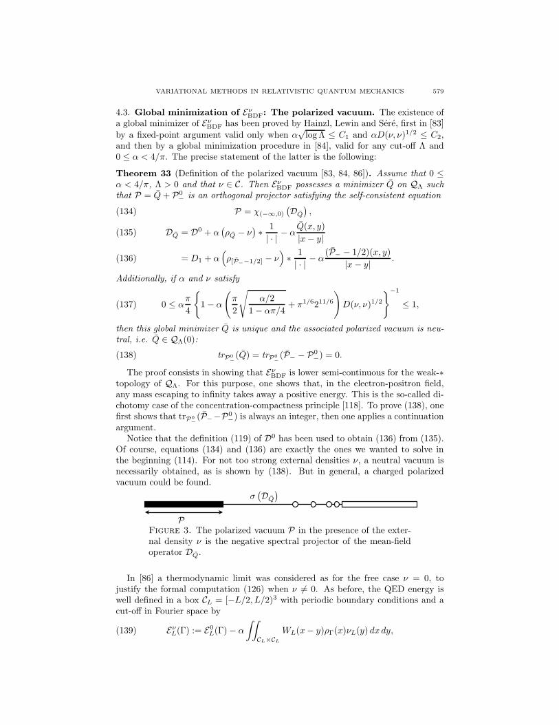
VARIATIONAL METHODS IN RELATIVISTIC QUANTUM MECHANICS 579
4.3. Global minimization of EνBDF: The polarized vacuum. The existence of
a global minimizer of EνBDF has been proved by Hainzl, Lewin and Sere, first in [83]
by a fixed-point argument valid only when α√
log Λ ≤ C1 and αD(ν, ν)1/2 ≤ C2,and then by a global minimization procedure in [84], valid for any cut-off Λ and0 ≤ α < 4/π. The precise statement of the latter is the following:
Theorem 33 (Definition of the polarized vacuum [83, 84, 86]). Assume that 0 ≤α < 4/π, Λ > 0 and that ν ∈ C. Then Eν
BDF possesses a minimizer Q on QΛ suchthat P = Q + P0
− is an orthogonal projector satisfying the self-consistent equation
P = χ(−∞,0)
(DQ
),(134)
DQ = D0 + α(ρQ − ν
)∗ 1| · | − α
Q(x, y)|x − y|(135)
= D1 + α(ρ[P−−1/2] − ν
)∗ 1| · | − α
(P− − 1/2)(x, y)|x − y| .(136)
Additionally, if α and ν satisfy
(137) 0 ≤ απ
4
1 − α
(π
2
√α/2
1 − απ/4+ π1/6211/6
)D(ν, ν)1/2
−1
≤ 1,
then this global minimizer Q is unique and the associated polarized vacuum is neu-tral, i.e. Q ∈ QΛ(0):
(138) trP0−(Q) = trP0
−(P− − P0
−) = 0.
The proof consists in showing that EνBDF is lower semi-continuous for the weak-∗
topology of QΛ. For this purpose, one shows that, in the electron-positron field,any mass escaping to infinity takes away a positive energy. This is the so-called di-chotomy case of the concentration-compactness principle [118]. To prove (138), onefirst shows that trP0
−(P−−P0
−) is always an integer, then one applies a continuationargument.
Notice that the definition (119) of D0 has been used to obtain (136) from (135).Of course, equations (134) and (136) are exactly the ones we wanted to solve inthe beginning (114). For not too strong external densities ν, a neutral vacuum isnecessarily obtained, as is shown by (138). But in general, a charged polarizedvacuum could be found.
σ(DQ
)P
Figure 3. The polarized vacuum P in the presence of the exter-nal density ν is the negative spectral projector of the mean-fieldoperator DQ.
In [86] a thermodynamic limit was considered as for the free case ν = 0, tojustify the formal computation (126) when ν = 0. As before, the QED energy iswell defined in a box CL = [−L/2, L/2)3 with periodic boundary conditions and acut-off in Fourier space by
(139) EνL(Γ) := E0
L(Γ) − α
∫∫CL×CL
WL(x − y)ρΓ(x)νL(y) dx dy,
580 MARIA J. ESTEBAN, MATHIEU LEWIN, AND ERIC SERE
where
(140) νL(x) =(2π)3/2
L3
∑k∈(2πZ3)/L
ν(k)eik·x
(for simplicity, it is assumed that ν is a smooth function). Then the following wasproved in [86].
Theorem 34 (Thermodynamic limit with external field [86]). Assume that 0 ≤α < 4/π, Λ > 0, ν ∈ C and that ν is continuous on B(0, Λ). Then for any L, Eν
L
possesses a minimizer ΓL = PL−ILΛ/2 on GL
Λ , where PL is an orthogonal projector,and one has
(141) limL→∞
Eν
L(ΓL) − E0L(Γ0
L)
= min EνBDF(Q), Q ∈ QΛ .
Moreover, up to a subsequence, QL(x, y) := (ΓL − Γ0L)(x, y) = (PL − P0
L)(x, y)converges uniformly on compact subsets of R
6 to Q(x, y), a minimizer of EνBDF on
QΛ.
Since all the previous results hold for any fixed Λ, it would be natural to considerthe limit Λ → ∞. This was done in [84] where it was argued that this limit is highlyunphysical: the vacuum polarization density totally cancels the external densityν. In QED, this “nullification” of the theory as the cut-off Λ diverges was firstsuggested by Landau [107] and later studied by Pomeranchuk et al. [133].
Notice that in QED, the procedure of renormalization is often used to formallyremove the cut-off Λ and the divergence of the theory. It consists in assumingthat the parameter α is not the physical one but the bare one. The physicalαphys 1/137 is related to α by a formula of the form
αphys α
1 + 2α log Λ/(3π).
When αphys is fixed at its physical value, then necessarily Λ ≤ 10280, meaningthat the large Λ limit should not be considered in principle. In the case where theexchange term is neglected in the energy (the so-called reduced BDF model), thisrenormalization procedure has been studied in detail in [84].
4.4. Minimization of EνBDF in charge sectors. The previous subsection was de-
voted to the global minimization of the BDF energy. We now mention some resultsthat have been obtained in [85] for minimization with a charge constraint. It isbelieved that the charge-constrained BDF model can be obtained as the thermo-dynamical limit of the full QED model in a fixed charge sector and posed in a boxwith periodic boundary conditions, but this has not been shown yet.
Due to the charge constraint and similarly for the Hartree-Fock model for in-stance, minimizers will not always exist for the BDF functional: It depends uponwhether the external electrostatic potential created by the charge distribution ν isstrong enough to be able to bind the N particles in the presence of the Dirac sea.On the other hand, it must not be too strong, otherwise electron-positron pairscould appear.
We start with a general result proved in [85] providing the form of a minimizer, ifit exists. To this end, we introduce the minimum energy in the N -th charge sector:
(142) Eν(N) := infEνBDF(Q) | Q ∈ QΛ, trP0
−(Q) = N
.

VARIATIONAL METHODS IN RELATIVISTIC QUANTUM MECHANICS 581
In principle N could be any real number, but here, for simplicity, we shall restrictourselves to integers.
Theorem 35 (Self-consistent equation of a BDF minimizer [85]). Let be 0 ≤ α <4/π, Λ > 0, ν ∈ C and N ∈ Z. Then any minimizer Q solution of the minimizationproblem (142), if it exists, takes the form Q = P − P0
−, where
(143) P = χ(−∞,µ](DQ) = χ(−∞,µ]
(D0 + α(ρQ − ν) ∗ 1/| · | − α
Q(x, y)|x − y|
),
for some µ ∈ [−m(α), m(α)].
Recall that m(α) is the threshold of the free operator D0 defined in (124). Weremark that (143) implicitly means that the last eigenvalue below µ of the mean-fieldoperator DQ is necessarily totally filled. As already mentioned in the Dirac-Fockcase, this is a general fact for Hartree-Fock type theories [7]. For a minimizer ofthe form (143) and when N, µ > 0, it is natural to consider the decomposition
P = Π + χ[0 , µ](DQ),
where Π is the polarized Dirac sea
Π := χ(−∞ , 0)(DQ).
For not too strong external potentials, the vacuum will be neutral, i.e.
trP0−(Π − P0
−) = 0 ,
and therefore χ[0 , µ](DQ) will be a projector of rank N
χ[0,µ](DQ) =N∑
n=1
ϕn ⊗ ϕ∗n, DQϕn = εnϕn ,
where ε1 ≤ · · · ≤ εN are the first N positive eigenvalues of DQ counted with theirmultiplicity. Notice that
(144) DQ = D1 + α(ρΦ − ν) ∗ 1| · | − α
γΦ(x, y)|x − y|
+ αρ[Π−IΛ/2] ∗1| · | − α
(Π − IΛ/2)(x, y)|x − y| ,
where
γΦ := χ[0,µ](DQ) =N∑
n=1
ϕn ⊗ ϕ∗n, ρΦ(x) := trC4(γΦ(x, x)) =
N∑n=1
|ϕn(x)|2.
In the first line of (144), the Dirac-Fock operator associated with (ϕ1, ..., ϕN ) ap-pears; see (95). This shows that the electronic orbitals ϕi are solutions of a Dirac-Fock type equation in which the mean-field operator DΦ is perturbed by the (self-consistent) potentials of the Dirac sea Π − IΛ/2. In practice, these potentials aresmall, and the DF equations are a good approximation of the BDF equations forthe electronic orbitals. But the energy functionals behave in a completely differentway: as we have seen, the DF energy is strongly indefinite while the BDF energyis bounded below. The Dirac-Fock model is thus interpreted as a nonvariationalapproximation of the mean-field model of no-photon QED [36].
Concerning the existence of a minimizer, solution of (143), the following resultwas proved in [85]:

582 MARIA J. ESTEBAN, MATHIEU LEWIN, AND ERIC SERE
σ (DQ)
Π ϕi’sP
µ
Figure 4. Decomposition of the system “vacuum + N electrons”for the solution P = Π + γΦ in the N -th charge sector.
Theorem 36 (Binding conditions and existence of a BDF minimizer [85]). Let0 ≤ α < 4/π, Λ > 0, ν ∈ C and N ∈ Z. Then the following two assertions areequivalent:
(H1) Eν(N) < minEν(N − K) + E0(K), K ∈ Z \ 0
.
(H2) Each minimizing sequence (Qn)n≥1 for Eν(N) is precompact in QΛ and con-verges, up to a subsequence, to a minimizer Q of Eν(N).
Conditions like (H1) appear classically when analyzing the compactness proper-ties of minimizing sequences, for instance by using the concentration-compactnessprinciple of P.-L. Lions [118]. They are also very classical for linear models inwhich the bottom of the essential spectrum has the form of the minimum in theright-hand side of (H1), as expressed by the HVZ Theorem [95, 163, 171]. AssumeN > 0 for simplicity. When 0 < K ≤ N , (H1) means that it is not favorable tolet K electrons escape to infinity, while keeping N − K electrons near the nuclei.When K < 0, it means that it is not favorable to let |K| positrons escape to infinity,while keeping N + |K| electrons near the nuclei. When K > N , it means that it isnot favorable to let K electrons escape to infinity, while keeping K − N positronsnear the nuclei. When α is small enough and N > 0, it was shown in [85] that theseparation of electron-positron pairs is not energetically favorable, so that one justneeds to check (H1) for K = 1, 2, ..., N .
To prove the existence of a minimizer, one can therefore prove that (H1) holds.Two situations in which (H1) is true have been provided by Hainzl, Lewin and Serein [85]. The first one is the case of weak coupling α 1 and αν = ν fixed (thecharge N is also fixed). The following was proved:
Theorem 37 (Existence of a minimizer in the weak coupling limit [85]). Assumethat Λ > 0, that N is a nonnegative integer, and that ν ∈ C is such that
(1) the spectrum σ(D0− ν ∗|·|−1) contains at least N positive eigenvalues below1,
(2) ker(D0 − tν ∗ | · |−1) = 0 for any t ∈ [0, 1].
Then (H1) holds in Theorem 36 for α small enough and αν = ν, and thereforethere exists a minimizer Qα of E ν/α(N). It takes the form
Qα = χ(−∞,0] (DQα) − P0
− + χ(0,µα] (DQα) := Qvac
α +N∑
i=1
|ϕαi 〉〈ϕα
i |,(145)
DQαϕα
i = εαi ϕα
i ,(146)
where εα1 ≤ · · · ≤ εα
N are the N first positive eigenvalues of DQα. Finally, for
any sequence αn → 0, (ϕαn1 , ..., ϕαn
N ) converges (up to a subsequence) in HΛ to
VARIATIONAL METHODS IN RELATIVISTIC QUANTUM MECHANICS 583
(ϕ1, ..., ϕN ) which are N first eigenfunctions of D0 − ν ∗ | · |−1 and Qvacαn
convergesto χ(−∞;0)
(D0 − ν ∗ | · |−1
)− P 0
− in S2(HΛ).
The second situation provided in [85] is the case of the nonrelativistic regimec 1. To state the result correctly, we reintroduce the speed of light c in themodel (of course, we shall then take α = 1). The expression of the energy andthe definition of the free vacuum P0
− (which of course then depends on c and theultraviolet cut-off Λ) are straightforward. We denote by Eν
α,c,Λ(N) the minimumenergy of the BDF functional depending on the parameters (α, c, Λ). The followingwas proved:
Theorem 38 (Existence of a minimizer in the nonrelativistic limit [85]). Assumethat α = 1 and that the ultraviolet cut-off is Λ = Λ0c for some fixed Λ0. Letν ∈ C ∩ L1(R3, R+) with
∫R3 ν = Z, and N a positive integer which is such that
Z > N − 1. Then, for c large enough, (H1) holds in Theorem 36 and thereforethere exists a minimizer Qc for Eν
1,c,Λ0c(N). It takes the form
Qc = χ(−∞,0)(DQ) − P0− + χ[0,µc)(DQ) = Qvac
c +N∑
i=1
|ϕci 〉〈ϕc
i | ,
and one has
limc→∞
Eν
1,c,Λ0c(N) − Ng0(0)
= minΦ∈H1(R3,C2)N
Gram Φ=EHF(Φ).
Moreover, for any sequence cn → ∞, (ϕcn1 , ..., ϕcn
N ) converges in H1(R3, C4)N (upto a subsequence) towards (ϕ1, ..., ϕN ) with ϕi =
(ϕi
0
), and where Φ0 = (ϕ1, ..., ϕN )
is a global minimizer of the Hartree-Fock energy.
We notice that this result is very similar to Theorem 26, providing the conver-gence of the Dirac-Fock “ground state” in the nonrelativistic limit.
4.5. Neglecting vacuum polarization: Mittleman’s conjecture. In view ofthe complications introduced by the Dirac sea, some authors [5, 6, 14] consideredan approximate model in which the vacuum polarization is neglected, in the spiritof a paper by Mittleman [125]. In this subsection, we shall keep the speed of lightc and therefore take α = 1.
In the vacuum case, a possible way to describe Mittleman’s approach is first towrite that the global minimizer P − 1/2 constructed in Theorem 33 is formally asolution of the following tautological max-min principle:
(147) e = supP
P 2=P
infγ
−P≤γ≤1−P
EνQED(P + γ) − Eν
QED(P )
.
Indeed taking γ = 0, one finds that e ≤ 0. Saying that P is a global QED minimizerexactly means that
minγ
−P≤γ≤1−P
EνQED(P + γ) − Eν
QED(P)
= 0.

584 MARIA J. ESTEBAN, MATHIEU LEWIN, AND ERIC SERE
Then, the idea is to approximate (147) by neglecting the vacuum polarization termscoming from P . Formally one has
(148) EνQED(P + γ) − Eν
QED(P ) = tr(DP γ) −∫∫
R3×R3
ργ(x)ν(y)|x − y| dx dy
+12
∫∫R3×R3
ργ(x)ργ(y)|x − y| dx dy − 1
2
∫∫R3×R3
|γ(x, y)|2|x − y| dx dy
withDP := Dc + ρ[P−1/2] ∗
1| · | −
(P − 1/2)(x, y)|x − y| .
Neglecting the vacuum polarization potentials then simply amounts to replacingDP by the free Dirac operator Dc. The following max-min principle was studiedby Bach, Barbaroux, Helffer and Siedentop in [6], inspired by Mittleman [125]:
(149) eν,cMitt = sup
P,P 2=P=P ∗
infγ∈S1(HΛ),−P≤γ≤1−P
Eν,cP (γ),
where Eν,cP is defined as
(150) Eν,cP (γ) := tr(Dcγ) − D(ν, ργ) +
12D(ργ , ργ) − 1
2
∫∫R6
|γ(x, y)|2|x − y| dx dy
on the set depending on P ,
Γ(P ) := γ ∈ S1(H), |∇|γ ∈ S1(H), −P ≤ γ ≤ 1 − P.The advantage of this formulation is that, since the vacuum polarization has beenneglected, no divergence problem is encountered and (149) can be studied withoutany Fourier cut-off (i.e. H = H1/2(R3, C4)), and with pointwise external charges(i.e. ν = Zδ0, where δ0 is the Dirac distribution at the point 0 ∈ R
3). The followingwas proved in [6]:
Theorem 39 (Mittleman principle for the vacuum [6]). Assume that ν = Zδ0 forsome Z ≥ 0 and that c > 0 satisfies 4c(1 − 2Z/c)/π ≥ 1. Then
Pc := χ(−∞,0)(Dc − Z/|x|)is the unique solution of Mittleman’s max-min principle
(151) eν,cMitt = sup
P∈Sinf
γ∈Γ(P )Eν,c
P (γ),
where S denotes the set of all the orthogonal projectors P which are such that Pand 1 − P leave the domain of Dc − Z/|x| invariant. Moreover, eν,c
Mitt = 0.
As a consequence, when vacuum polarization is neglected, the Dirac sea is rep-resented by the negative spectral projector of the operator Dc − Z/|x|.
The N electron case was studied by Mittleman in [125]. His main idea was tojustify the validity of the Dirac-Fock approximation by a type of max-min principlefrom QED in which vacuum polarization is neglected. Let us introduce the followingmax-min principle:
(152) eν,cMitt(N) = sup
P∈Sinf
γ∈Γ(P )γP=Pγ,tr(γ)=N
Eν,cP (γ).
The interpretation is that γ represents the N electrons, whereas P is the Diracsea. Notice that in this interpretation, the real particles are artificially separated
VARIATIONAL METHODS IN RELATIVISTIC QUANTUM MECHANICS 585
from the virtual electrons of the Dirac sea. However, it was believed that (152)could be a simpler problem with interesting practical implications. We remark thatcompared to (149), we have added in (152), the condition that γ commutes withP , i.e. it cannot contain off-diagonal terms. Without this requirement, it is known[4] that (152) cannot give any solution of the Dirac-Fock equations.
Mittleman’s conjecture consists in saying that the max-min principle (152) isattained by a solution to the Dirac-Fock system. More precisely, we follow [13] andstate it as:
Mittleman’s conjecture. A solution of (152) is given by a pair
(P, γ) = (χ(−∞,0)(Dc,Φ), γΦ),
where Φ is a solution of the Dirac-Fock equation Dc,Φϕi = εiϕi with εi > 0, andwhere Dc,Φ is the Dirac-Fock mean-field operator defined in (95).
Mittleman’s conjecture for molecules has been investigated in [14, 13]. In [14]Barbaroux, Farkas, Helffer and Siedentop studied the minimization problem onΓ(P ) in (152) for a fixed P . Under suitable conditions, they proved that γ is anelectronic density matrix γ =
∑Ni=1 |ϕi〉〈ϕi|, where (ϕ1, ..., ϕN ) is a solution of the
projected Dirac-Fock equations (1 − P )Dc,Φ(1 − P )ϕi = εiϕi. Then they furtherproved that if the energy is stationary with respect to variations of the projectorP , then the unprojected Dirac-Fock equations are obtained. But they were unableto prove the existence of such a state.
In [13], Barbaroux, Esteban and Sere investigated the validity of Mittleman’sconjecture by a perturbation argument. Namely they added a parameter τ in frontof the interaction terms as follows:
(153) Eν,c,τP (γ) := tr(Dcγ) − D(ν, ργ) +
τ
2D(ργ , ργ) − τ
2
∫∫R6
|γ(x, y)|2|x − y| dx dy.
Here ν is a fixed positive and smooth radial function with compact support and∫R3 ν = 1. They studied Mittleman’s conjecture in the regime c 1 and τ 1. We
emphasize that by a scaling argument this physically corresponds to assuming α 1 and Z 1 with αZ 1. We denote by Eν,c,τ
DF the Dirac-Fock functional whichis easily defined with these parameters, and by Φc,τ,0 the DF solution obtained bythe corresponding versions of Theorems 23 and 27 for j = 0.
When c > 1, it is known that Dc−ν∗|·|−1 is essentially self-adjoint on L2(R3, C4)and that its spectrum is
σ(Dc − ν ∗ | · |−1) = (−∞,−c2] ∪ µ1(c) < µ2(c) · · · ∪ [c2,∞),
where limi→∞ µi(c) = c2. We denote by (Ni(c))i≥1 the multiplicities of the µi(c)’s.The following was proved in [13]:
Theorem 40 (Validity and nonvalidity of Mittleman’s conjecture [13]). Assumethat ν is a fixed positive and smooth radial function with compact support and suchthat
∫R3 ν = 1.
If N =∑I
i=1 Ni(c) for some I ≥ 1 and some fixed c > 1, then Mittleman’sconjecture is true for τ small enough: one has
eν,c,τMitt (N) = Eν,c,τ
DF (Φc,τ,0) ,
where Φc,τ,0 is any of the solutions obtained in Theorem 23 in the case j = 0.Moreover, the optimal projector for the sup part of (152) is P = χ(−∞,0)(Dc,Φc,τ,0).

586 MARIA J. ESTEBAN, MATHIEU LEWIN, AND ERIC SERE
If N =∑I
i=1 Ni(c)+1 for some I ≥ 1 and c large enough, then Mittleman’s con-jecture is wrong when τ > 0 is small enough: there is no solution Φ of the Dirac-Fock equations with positive multipliers such that the pair
(χ(−∞,0)(Dc,Φ), γΦ
)re-
alizes Mittleman’s max-min principle (152).
One can consider a weaker version of Mittleman’s conjecture which consists inonly comparing energy levels and not the solutions themselves.
Wealer Mittleman’s conjecture. One has
eν,c,τMitt (N) = Eν,c,τ
DF (Φc,τ,0).
When N = 1 and for c 1, τ 1, it is known by Theorem 40 that Mittleman’sconjecture is wrong. But Barbaroux, Helffer and Siedentop proved in [15] that theweaker conjecture is indeed true.
Theorem 41 (Validity of the weaker Mittleman conjecture for N = 1 [15]). Assumethat ν = δ0. Then for c large enough and τ small enough, the weaker Mittlemanconjecture is true:
eν,c,τMitt (N) = Eν,c,τ
DF (Φc,τ,0).The sup-inf principle (152) is realized by the pair(
Pc, γ)
with Pc = χ(−∞,0)(Dc − 1/|x|), γ = |ϕc〉〈ϕc|,where ϕc is any eigenvector of
(154) Dc − 1/|x|with eigenvalue eν,c,τ
Mitt (N).
In [15], an explicit condition on τ and c is provided. Notice the equality
Dc,ϕϕc = Dc,0ϕc = (Dc − 1/|x|)ϕc = eν,c,τ
Mitt (N)ϕc,
which is very specific to the one-electron case, and means that the electron doesnot “see” its own Coulomb field. In particular Pcϕ
c = 0.For N ≥ 2, the question remains completely open.
Acknowledgments
First of all, M.J.E. and E.S. would like to thank T. Cazenave, I. Ekeland, P.-L.Lions and L. Vazquez for having introduced them to this field. We would like alsoto thank J. Dolbeault, V. Georgiev, C. Hainzl, M. Loss and J.-P. Solovej with whomwe have collaborated on differents parts of the works described in this review. Someyears ago P. Chaix was very patient in explaining to us some models of QED onwhich we have worked later; the last section of this paper has its origin in thoseconversations. Several discussions with B. Buffoni were very inspiring to us whenlooking for new variational principles in the case of strongly indefinity functionals.We want also to acknowledge our participation in the European research projects“Analysis and Quantum” (HPRN-CT-2002-00277) and “HYKE” (HPRN-CT-2002-00282). The interaction with our partners in those two projects has been a source ofinspiration and motivation for us along the years, and we thank them for that. Wealso acknowledge support from the ANR “ACCQUAREL” of the French ministryof research. E.S. was partially supported by the Institut Universitaire de France.Finally, we wish to thank P. Rabinowitz, who has been very patient encouragingus to write this review article.
VARIATIONAL METHODS IN RELATIVISTIC QUANTUM MECHANICS 587
References
[1] S. Abenda. Solitary waves for Maxwell-Dirac and Coulomb-Dirac models. Ann. Inst. H.Poincare, Phys. Theor. 68(2) (1998), 229–244. MR1618672 (99c:81023)
[2] H. Amann. Saddle points and multiple solutions of differential equations. Math. Z. 169(1979), 127–166. MR550724 (80j:47078)
[3] C.D. Anderson. The Positive Electron. Phys. Rev. 43 (1933), 491–494.[4] W.H. Aschbacher. Lowering the Hartree-Fock minimizer by electron-positron pair correla-
tion. Lett. Math. Phys. 70(1), (2004), 29–41. MR2107703 (2006b:81064)[5] V. Bach, J.M. Barbaroux, B. Helffer, H. Siedentop. Stability of matter for the Hartree-
Fock functional of the relativistic electron-positron field. Doc. Math. 3 (1998), 353–364.MR1668924 (2001a:81082)
[6] V. Bach, J.M. Barbaroux, B. Helffer, H. Siedentop. On the stability of the relativis-tic electron-positron field. Comm. Math. Phys. 201(2) (1999), 445–460. MR1682210(2000i:81169)
[7] V. Bach, E.H. Lieb, M. Loss, J.P. Solovej. There are no unfilled shells in unrestricted Hartree-Fock theory. Phys. Rev. Lett. 72(19) (1994), 2981–2983.
[8] A. Bachelot. Probleme de Cauchy global pour des systemes de Dirac-Klein-Gordon. Ann.Inst. H. Poincare 48 (1988), 387–422. MR969173 (90i:81024)
[9] A. Bachelot-Motet. Nonlinear Dirac fields on the Schwarzschild metric. Classical QuantumGravity 15 (1998), 1815–1825. MR1633146 (99e:83010)
[10] A. Bahri, J.-M. Coron. On a nonlinear elliptic equation involving the critical Sobolev ex-ponent: the effect of the topology of the domain. Comm. Pure Appl. Math. 41(3) (1988),253–294. MR929280 (89c:35053)
[11] M. Balabane, T. Cazenave, A. Douady, F. Merle. Existence of excited states for a nonlinearDirac field. Comm. Math. Phys. 119 (1988), 153–176. MR968485 (90b:35195)
[12] M. Balabane, T. Cazenave, L. Vazquez. Existence of standing waves for Dirac fields withsingular nonlinearities. Comm. Math. Phys. 133 (1990), 53–74. MR1071235 (91k:81025)
[13] J.-M. Barbaroux, M. J. Esteban, E. Sere. Some connections between Dirac-Fock andelectron-positron Hartree-Fock. Ann. Henri Poincare 6(1) (2005), 85–102. MR2119356(2006b:81065)
[14] J.-M. Barbaroux, W. Farkas, B. Helffer, H. Siedentop. On the Hartree-Fock Equationsof the Electron-Positron Field. Comm. Math. Phys. 255 (2005), 131–159. MR2123379(2006c:81227)
[15] J.-M. Barbaroux, B. Helffer, H. Siedentop. Remarks on the Mittleman max-min varia-tional method for the electron-positron field. J. Phys. A 39(1) (2006), 85–98. MR2200186(2007d:81060)
[16] W.E. Bayliss, S. J. Peel. Stable variational calculations with the Dirac Hamiltonian. Phys.Rev. A, 28(4) (1983), 2552–2554.
[17] V. Benci, P.H. Rabinowitz. Critical point theorems for indefinite functionals. Inv. Math. 52(1979), 336–352. MR537061 (80i:58019)
[18] A. Berthier, V. Georgescu. Sur le spectre ponctuel de l’operateur de Dirac. C. R. Acad.Sci. Paris, Ser. A 297 (1983), p. 335–338. MR732500 (86f:35137)
[19] A. Berthier, V. Georgescu. On the point spectrum for Dirac operators. J. Funct. Anal. 71(1987), 309–338. MR880983 (89b:35131)
[20] J.D. Bjorken, S.D. Drell. Relativistic quantum fields. McGraw-Hill (1965). MR0187642(32:5092)
[21] N. Boussaid. Stable directions for small nonlinear Dirac standing waves. Comm. Math. Phys.268(3) (2006), 757–817. MR2259214
[22] N. Bournaveas. Local existence for the Maxwell-Dirac equations in three space dimensions.Comm. Partial Differential Equations 21(5–6) (1996), 693–720. MR1391520 (97f:35176)
[23] N. Bournaveas. Local existence of energy class solutions for the Dirac-Klein-Gordon equa-tions. Comm. Partial Differential Equations 24(7–8) (1999), 1167–1193. MR1697486(2000e:35188)
[24] H. Booth. Electrons with self-field as solutions to nonlinear PDE. Geometric analysis andapplications (Canberra, 2000), 1–14, Proc. Centre Math. Appl. Austral. Nat. Univ., 39,Austral. Nat. Univ., Canberra, 2001. MR1852690 (2002h:81104)

588 MARIA J. ESTEBAN, MATHIEU LEWIN, AND ERIC SERE
[25] H. Brezis, L. Nirenberg. Positive solutions of nonlinear elliptic equations involving crit-ical Sobolev exponents. Comm. Pure Appl. Math. 36(4) (1983), 437–477. MR709644(84h:35059)
[26] B. Buffoni, M.J. Esteban, E. Sere. Normalized solutions to strongly indefinite semilinearequations. Adv. Nonlinear Stud. 6(2) (2006), 323–347. MR2219842 (2007e:35072)
[27] B. Buffoni, L. Jeanjean. Minimax characterization of solutions for a semi-linear ellipticequation with lack of compactness. Ann. Inst. H. Poincare Anal. Non Lineare 10(4) (1993),
377–404. MR1246458 (94m:35099)[28] B. Buffoni, L. Jeanjean, C. A. Stuart. Existence of a nontrivial solution to a strongly in-
definite semilinear equation. Proc. Amer. Math. Soc. 119(1) (1993), 179–186 MR1145940(93k:35086)
[29] V.I. Burenkov, W.D. Evans. On the evaluation of the norm of an integral operator associatedwith the stability of one-electron atoms. Proc. Roy. Soc. Edinburgh, Sect. A 128(5) (1998),993–1005. MR1642120 (99i:47091)
[30] E. Cances, A. Deleurence, M. Lewin. A new approach to the modelling of local defects incrystals: the reduced Hartree-Fock case. Comm. Math. Phys., 281 (2008), 129–177.
[31] A. Castro, A.C. Lazer. Applications of a min-max principle. Rev. Colombiana Mat. 10(1976), 141–149. MR0501089 (58:18544)
[32] T. Cazenave. On the existence of stationary states for classical nonlinear Dirac fields. InHyperbolic systems and Mathematical Physics. Textos e Notas 4, CMAF, Lisbonne (1989).
[33] T. Cazenave, L. Vazquez. Existence of localized solutions for a classical nonlinear Dirac field.Comm. Math. Phys. 105 (1986), 35–47. MR847126 (87j:81027)
[34] J. Chadam. Global solutions of the Cauchy problem for the (classical) coupled Maxwell-Dirac system in one space dimension. J. Funct. Anal. 13 (1973), 173–184. MR0368640(51:4881)
[35] J. Chadam, R. Glassey. On the Maxwell-Dirac equations with zero magnetic field and theirsolutions in two space dimensions. J. Math. Anal. Appl. 53 (1976), 495–507. MR0413833(54:1947)
[36] P. Chaix, D. Iracane. The Bogoliubov-Dirac-Fock formalism. I. J. Phys. At. Mol. Opt. Phys.22 (1989), 3791–3814.
[37] P. Chaix, D. Iracane, P.-L. Lions. The Bogoliubov-Dirac-Fock formalism. II. J. Phys. At.Mol. Opt. Phys. 22 (1989), 3815–3828.
[38] Y. Choquet-Bruhat. Solutions globales des equations de Maxwell-Dirac-Klein-Gordon(masses nulles). C. R. Acad. Sci. Paris, Serie I 292 (1981), 153–158. MR610307 (82f:81037)
[39] F.H. Clarke, I. Ekeland. Hamiltonian trajectories having prescribed minimal period. Comm.Pure Appl. Math. 33(2) (1980), 103–116. MR562546 (81e:70017)
[40] C.V. Coffman. Uniqueness of the ground state solution for ∆u−u+u3 = 0 and a variationalcharacterization of other solutions. Arch. Rat. Mech. Anal. 46 (1972), 81–95. MR0333489(48:11814)
[41] C. Conley, E. Zehnder. The Birkhoff-Lewis fixed point theorem and a conjecture of V.I.Arnold. Invent. Math. 73 (1983), 33–49. MR707347 (85e:58044)
[42] S.N. Datta, G. Deviah. The minimax technique in relativistic Hartree-Fock calculations.Pramana 30(5) (1988), 393–416.
[43] J.P. Dias, M. Figueira. Global existence of solutions with small initial data in Hs for themassive nonlinear Dirac equations in three space dimensions. Boll. Unione Mat. Ital. B (7)1(3) (1987), 861–874. MR916298 (89f:35181)
[44] P.A.M. Dirac. The quantum theory of the electron. Proc. Roy. Soc. A 117 (1928), 610–624.[45] P.A.M. Dirac. A theory of electrons and protons. Proc. Roy. Soc. A 126 (1930), 360–365.[46] P.A.M. Dirac. Theorie du positron. Solvay report (1934), 203–212. Gauthier-Villars, Paris.
XXV, 353 S.[47] P.A.M. Dirac. Discussion of the infinite distribution of electrons in the theory of the positron.
Proc. Camb. Philos. Soc. 30 (1934), 150–163.[48] J. Dolbeault, M.J. Esteban, M. Loss. Relativistic hydrogenic atoms in strong magnetic fields.
Ann. Henri Poincare 8(4) (2007), 749–779. MR2333781[49] J. Dolbeault, M.J. Esteban, M. Loss, L. Vega. An analytical proof of Hardy-like inequalities
related to the Dirac operator. J. Funct. Anal. 216 (2004), 1–21. MR2091354 (2005h:35291)
VARIATIONAL METHODS IN RELATIVISTIC QUANTUM MECHANICS 589
[50] J. Dolbeault, M.J. Esteban, E. Sere. Variational characterization for eigenvalues of Diracoperators. Calc. Var. Partial Differential Equations 10 (2000), 321–347. MR1767717(2001f:49083)
[51] J. Dolbeault, M.J. Esteban, E. Sere. On the eigenvalues of operators with gaps. Applicationto Dirac operators. J. Funct. Anal. 174 (2000), 208–226. MR1761368 (2001e:47040)
[52] J. Dolbeault, M.J. Esteban, E. Sere. A variational method for relativistic computations inatomic and molecular physics. Int. J. Quantum Chemistry 93 (2003), 149–155.
[53] J. Dolbeault, M. J. Esteban, E. Sere. General results on the eigenvalues of operators withgaps, arising from both ends of the gaps. Application to Dirac operators. J. Eur. Math. Soc.8(2) (2006), 243–251. MR2239275 (2007m:47044)
[54] J. Dolbeault, M.J. Esteban, E. Sere, M. Vanbreugel. Minimization methods for the one-particle Dirac equation. Phys. Rev. Lett. 85(19) (2000), 4020–4023.
[55] G.W.F. Drake, S.P. Goldman. Application of discrete-basis-set methods to the Dirac equa-tion. Phys. Rev. A 23 (1981), 2093–2098.
[56] G.W.F. Drake, S.P. Goldman. Relativistic Sturmian and finite basis set methods in atomicphysics. Adv. Atomic Molecular Phys. 23 (1988), 23–29.
[57] G.W.F. Drake, S.P. Goldman. Adv. Atomic Molecular Phys. 25 (1988), 393.[58] Ph. Durand. Transformation du Hamiltonien de Dirac en Hamiltoniens variationnels de
type Pauli. Application a des atomes hydrogenoıdes. C. R. Acad. Sci. Paris 303(2) (1986),119–124.
[59] Ph. Durand, J.-P. Malrieu. Effective Hamiltonians and pseudo-potentials as tools for rigorousmodelling. In Ab initio methods in Quantum Chemistry I. K.P. Lawley ed., J. Wiley & Sons,1987.
[60] M. Escobedo, L. Vega. A semilinear Dirac equation in Hs(R3) for s > 1. SIAM J. Math.Anal. 28(2) (1997), 338–362. MR1434039 (97k:35239)
[61] M.J. Esteban, V. Georgiev, E. Sere. Stationary solutions of the Maxwell-Dirac and theKlein-Gordon-Dirac equations. Cal. Var. Partial Differential Equations 4 (1996), 265–281.MR1386737 (97g:35144)
[62] M.J. Esteban, E. Sere. Stationary states of the nonlinear Dirac equation: a variationalapproach. Comm. Math. Phys. 171 (1995), 323–350. MR1344729 (96g:81041)
[63] M.J. Esteban, E. Sere. Existence and multiplicity of solutions for linear and nonlinear Diracproblems. Partial Differential Equations and Their Applications. CRM Proceedings andLecture Notes, vol. 12. Eds. P.C. Greiner, V. Ivrii, L.A. Seco and C. Sulem. AMS, 1997.
[64] M.J. Esteban, E. Sere. Solutions for the Dirac-Fock equations for atoms and molecules.Comm. Math. Phys. 203 (1999), 499–530. MR1700174 (2000j:81057)
[65] M.J. Esteban, E. Sere. Nonrelativistic limit of the Dirac-Fock equations. Ann. HenriPoincare 2 (2001), 941–961. MR1869528 (2003d:81066)
[66] M.J. Esteban, E. Sere. A max-min principle for the ground state of the Dirac-Fock functional.Contemp. Math. 307 (2002), 135–141. MR1946024 (2003k:81052)
[67] W.D. Evans, P. Perry, H. Siedentop. The spectrum of relativistic one-electron atoms ac-cording to Bethe and Salpeter. Comm. Math. Phys. 178 (1996), 733–746. MR1395212(97e:81019)
[68] G. Fang, N. Ghoussoub. Morse-type information on Palais-Smale sequences obtained bymin-max principles. Comm. Pure Appl. Math. 47(12) (1994), 1595–1653. MR1303222(95m:58028)
[69] R. Finkelstein, R. Lelevier, M. Ruderman. Nonlinear spinor fields. Phys. Rev. 83 (1951),326–332. MR0042204 (13:76b)
[70] R. Finkelstein, C. Fronsdal, P. Kaus. Nonlinear Spinor Field. Phys. Rev. 103 (1956), 1571–1579.
[71] F. Finster, J. Smoller, S.-T. Yau. Particle-like solutions of the Einstein-Dirac-Maxwell equa-tions. Phys. Lett. A. 259(6) (1999), 431–436. MR1714646 (2000f:83016)
[72] F. Finster, J. Smoller, S.-T. Yau. Non-existence of black hole solutions for a sphericallysymmetric, static Einstein-Dirac-Maxwell system. Comm. Math. Phys. 205(2) (1999), 249–
262. MR1712611 (2000k:83008)[73] M. Flato, J. Simon, E. Taflin. On the global solutions of the Maxwell-Dirac equations.
Comm. Math. Phys. 113 (1987), 21–49. MR904136 (88k:35117)[74] A. Floer. Morse theory for fixed points of symplectic diffeomorphisms. Bull. Amer. Math.
Soc. 16(2) (1987), 279–281. MR876964 (88b:58024)

590 MARIA J. ESTEBAN, MATHIEU LEWIN, AND ERIC SERE
[75] L.L. Foldy, E. Eriksen. Some physical consequences of vacuum polarization. Phys. Rev.95(4) (1954), 1048–1051.
[76] V. Georgiev. Small amplitude solutions of the Maxwell-Dirac equations. Indiana Univ. Math.J. 40(3) (1991), 845–883. MR1129332 (92i:81107)
[77] N. Ghoussoub. Duality and perturbation methods in critical point theory. Cambridge Univ.Press, 1993. MR1251958 (95a:58021)
[78] R. Glauber, W. Rarita, P. Schwed. Vacuum polarization effects on energy levels in µ-mesonic
atoms. Phys. Rev. 120(2) (1960), 609–613.[79] W.T. Grandy, Jr. Relativistic quantum mechanics of leptons and fields. Kluwer Acad.
Publisher, Fund. Theories of Physics, Vol. 41.[80] M. Griesemer, R.T. Lewis, H. Siedentop. A minimax principle in spectral gaps: Dirac op-
erators with Coulomb potentials. Doc. Math. 4 (1999), 275–283 (electronic). MR1701887(2000g:47023)
[81] M. Griesemer, H. Siedentop. A minimax principle for the eigenvalues in spectral gaps. J.London Math. Soc. 60(2) (1999), 490–500. MR1724845 (2000i:47047)
[82] L. Gross. The Cauchy problem for the coupled Maxwell and Dirac equations. Comm. PureAppl. Math. 19 (1966), 1–5. MR0190520 (32:7932)
[83] C. Hainzl, M. Lewin, E. Sere. Existence of a stable polarized vacuum in the Bogoliubov-Dirac-Fock approximation. Comm. Math. Phys. 257(3) (2005), 515–562. MR2164942(2006i:81123)
[84] C. Hainzl, M. Lewin, E. Sere. Self-consistent solution for the polarized vacuum in a no-photonQED model, J. Phys. A: Math. and Gen. 38 (2005), 4483–4499. MR2147635 (2006e:81341)
[85] C. Hainzl, M. Lewin, E. Sere. Existence of atoms and molecules in the mean-field approxi-mation of no-photon Quantum Electrodynamics, Arch. Rat. Mech. Anal., to appear.
[86] C. Hainzl, M. Lewin, J.P. Solovej. The mean-field approximation in Quantum Electrody-namics. The no-photon case. Comm. Pure Appl. Math. 60(4) (2007), 546–596. MR2290710
[87] C. Hainzl, M. Lewin, E. Sere, J.P. Solovej. A minimization method for relativistic electrons ina mean-field approximation of Quantum Electrodynamics. Phys. Rev. A 76 (2007), 052104.
[88] C. Hainzl, M. Lewin, C. Sparber. Existence of global-in-time solutions to a generalizedDirac-Fock type evolution equation, Lett. Math. Phys. 72 (2005), 99–113. MR2154857(2006b:81070)
[89] W. Heisenberg. Bemerkungen zur Diracschen Theorie des Positrons. Z. Phys. 90 (1934),209–223.
[90] W. Heisenberg. Doubts and hopes in quantum electrohydrodynamics. Physica 19 (1953),897–908. MR0058472 (15:378f)
[91] I.W. Herbst. Spectral theory of the operator (p2 +m2)1/2 −Ze2/r. Comm. Math. Phys. 53
(1977), 285–294. MR0436854 (55:9790)[92] R.N. Hill, C. Krauthauser. A solution to the problem of variational collapse for the one-
particle Dirac equation. Phys. Rev. Lett. 72(14) (1994), 2151–2154.[93] H. Hofer, K. Wysocki. First order elliptic systems and the existence of homoclinic orbits in
Hamiltonian systems. Math. Ann. 288 (1990), 483–503. MR1079873 (91m:58064)[94] M. Huber, H. Siedento Solutions of the Dirac-Fock equations and the energy of the electron-
positron field. Arch. Rat. Mech. Anal. 184 (1) (2007), 1–22. MR2289861 (2007m:81065)[95] W. Hunziker. On the spectra of Schrodinger multiparticle Hamiltonians. Helv. Phys. Acta.
39 (1966), 451–462. MR0211711 (35:2588)[96] W. Hunziker, I.M. Sigal. The quantum N-body problem. J. Math. Phys. 41(6) (2000),
3448–3510. MR1768629 (2001g:81267)[97] D. Ivanenko. Soviet Physics 13 (1938), 141–149.[98] T. Kato. Perturbation theory for linear operators. Springer, 1966.[99] T. Kato. Holomorphic families of Dirac operators. Math. Z. 183(3) (1983), 399–406.
MR706397 (84k:35114)[100] S. Klainerman. Global existence of small amplitude solutions to the nonlinear Klein-
Gordon equations in four space dimensions. Comm. Pure Appl. Math. 38 (1985), 631–641.MR803252 (87e:35080)
[101] S. Klainerman. The null condition and global existence to nonlinear wave equations. Lect.in Appl. Math. 23 (1986), 293–326. MR837683 (87h:35217)
[102] S. Klainerman. Remarks on the global Sobolev inequalities in the Minkowski space Rn+1.Comm. Pure Appl. Math. 40 (1986), 111–117. MR865359 (88a:46035)

VARIATIONAL METHODS IN RELATIVISTIC QUANTUM MECHANICS 591
[103] M. Klaus, R. Wust. Characterization and uniqueness of distinguished self-adjoint extensionsof Dirac operators. Comm. Math. Phys. 64(2) (1978-79), 171–176. MR519923 (80k:81025)
[104] W. Kutzelnigg. Basis set expansion of the Dirac operator without variational collapse. Int.J. Quant. Chem. 25 (1984), 107–129.
[105] W. Kutzelnigg. Relativistic one-electron Hamiltonians “for electrons only” and the varia-tional treatment of the Dirac equation. Chemical Physics 225 (1997), 203–222.
[106] M.K. Kwong, Y. Li. Uniqueness of radial solutions of semilinear elliptic equations. Trans.
Amer. Math. Soc. 333 (1992), 339–363. MR1088021 (92k:35102)[107] L.D. Landau. On the quantum theory of fields. Bohr Volume, Pergamon Press, Oxford, 1955.
Reprinted in Collected papers of L.D. Landau, edited by D. Ter Haar, Pergamon Press, 1965.MR0075092 (17:692f)
[108] C. Le Bris, P.-L. Lions. From atoms to crystals: a mathematical journey. Bull. Amer. Math.Soc. (N.S.) 42(3) (2005), 291–363. MR2149087 (2006k:81121)
[109] E. van Lenthe, E.J. Baerends, J.G. Snijders. Solving the Dirac equation, using the largecomponent only, in a Dirac-type Slater orbital basis set. Chem. Phys. Lett. 236 (1995),235-241.
[110] E. van Lenthe, R. van Leeuwen, E.J. Baerends, J.G. Snijders. Relativistic regular two-component Hamiltonians. In New challenges in computational Quantum Chemistry. R.Broek et al ed. Publications Dept. Chem. Phys. and Material sciences. University of Gronin-gen, 1994.
[111] R. van Leeuwen, E. van Lenthe, E.J. Baerends, J.G. Snijders. Exact solutions of regularapproximate relativistic wave equations for hydrogen-like atoms. J. Chem. Phys. 101(2)(1994), 1272–1281.
[112] A. Le Yaouanc, L. Oliver, J.-C. Raynal. The Hamiltonian (p2 + m2)1/2 − α/r near thecritical value αc = 2/π. J. Math. Phys. 38(8) (1997), 3397–4012. MR1459640 (98g:81033)
[113] E.H. Lieb. Variational principle for many-fermion systems. Phys. Rev. Lett. 46 (1981), 457–459. MR601336 (81m:81083)
[114] E.H. Lieb. On the lowest eigenvalue of the Laplacian for the intersection of two domains.Invent. Math. 74(3) (1983), 441–448. MR724014 (85e:35090)
[115] E.H. Lieb. Bound on the maximum negative ionization of atoms and molecules. Phys. Rev.A. 29 (1984), 3018–3028.
[116] E.H. Lieb, H. Siedentop. Renormalization of the regularized relativistic electron-positronfield. Comm. Math. Phys. 213(3) (2000), 673–683. MR1785433 (2001i:81175)
[117] E. H. Lieb, B. Simon. The Hartree-Fock theory for Coulomb systems. Comm. Math. Phys.,53 (1977), 185–194. MR0452286 (56:10566)
[118] P.-L. Lions. The concentration-compactness method in the Calculus of Variations. The lo-cally compact case. Part. I: Ann. Inst. H. Poincare Anal. Nonlineaire 1 (1984), 109–145.Part. II: Ann. Inst. H. Poincare Anal. Nonlineaire 1 (1984), 223–283.
[119] P.-L. Lions. Solutions of Hartree-Fock equations for Coulomb systems. Comm. Math. Phys.109 (1987), 33–97. MR879032 (88e:35170)
[120] A.G. Lisi. A solitary wave solution of the Maxwell-Dirac equations. J. Phys. A 28(18)(1995), 5385–5392. MR1364144 (96k:81079)
[121] S. Machihara, K. Nakanishi, T. Ozawa. Small global solutions and the nonrelativistic limit forthe nonlinear Dirac equation. Rev. Mat. Iberoamericana 19(1) (2003), 179–194. MR1993419
(2005h:35293)[122] N. Masmoudi, K. Nakanishi. Nonrelativistic limit from Maxwell-Klein-Gordon and Maxwell-
Dirac to Poisson-Schrodinger. Int. Math. Res. Not. 13 (2003), 697–734. MR1949296(2004b:81042)
[123] N. Masmoudi, K. Nakanishi. Uniqueness of Finite Energy Solutions for Maxwell-Dirac andMaxwell-Klein-Gordon Equations. Comm. Math. Phys. 243 (2003), 123–136. MR2020223(2004i:81060)
[124] F. Merle. Existence of stationary states for nonlinear Dirac equations. J. Differential Equa-tions 74(1) (1988), 50–68. MR949625 (89k:81027)
[125] M.H. Mittleman. Theory of relativistic effects on atoms: Configuration-space Hamiltonian.Phys. Rev. A 24(3) (1981), 1167–1175.
[126] P. J. Mohr, G. Plunien, G. Soff. QED corrections in heavy atoms. Phys. Rep. 293(5&6)(1998), 227–372.
592 MARIA J. ESTEBAN, MATHIEU LEWIN, AND ERIC SERE
[127] B. Najman. The nonrelativistic limit of the nonlinear Dirac equation. Ann. Inst. H. PoincareAnal. Non Lineaire 9(1) (1992), 3–12. MR1151464 (93b:81047)
[128] G. Nenciu. Self-adjointness and invariance of the essential spectrum for Dirac operatorsdefined as quadratic forms. Comm. Math. Phys. 48 (1976), 235–247. MR0421456 (54:9459)
[129] G. Nenciu. Existence of spontaneous pair creation in the external field approximation ofQ.E.D., Comm. Math. Phys. 109 (1987), 303–312. MR880417 (89b:81271)
[130] H. Ounaies. Perturbation method for a class of nonlinear Dirac equations. Differential In-
tegral Equations 13(4-6) (2000), 707–720. MR1750047 (2001a:35150)[131] E. Paturel. Solutions of the Dirac equations without projector. Ann. Henri Poincare 1
(2000), 1123–1157. MR1809795 (2001k:81369)[132] P. Pickl. Existence of Spontaneous Pair Creation. Dissertiation, Munchen (2005),
arXiv:hep-th/0609200.[133] I.Ya Pomeranchuk, V.V. Sudakov, K.A. Ter-Martirosyan. Vanishing of renormalized charges
in field theories with point interaction. Phys. Rev. 103 (3) (1956), 784–802. MR0082374(18:541a)
[134] P.H. Rabinowitz. Free vibrations for a semilinear wave equation. Comm. Pure Appl. Math.31(1) (1978), 31–68. MR470378 (81i:35109)
[135] P.H. Rabinowitz. Periodic solutions of Hamiltonian systems. Comm. Pure Appl. Math. 31(2)(1978), 157–184. MR0467823 (57:7674)
[136] C.J. Radford. Localized solutions of the Dirac-Maxwell equations. J. Math. Phys. 37(9)(1996), 4418–4433. MR1408100 (97g:81076)
[137] C.J. Radford. The stationary Maxwell-Dirac equations. J. Phys. A 36(20) (2003), 5663–5681. MR1985533 (2004i:81268)
[138] A.F. Ranada. Classical nonlinear Dirac field models of extended particles. In Quantumtheory, groups, fields and particles (editor A.O. Barut). Reidel, Amsterdam (1982).
[139] M. Reed. Abstract non-linear wave equations. Lecture Notes in Math. 507, Springer-Verlag,Berlin, 1976. MR0605679 (58:29290)
[140] M. Reed, B. Simon. Methods of modern mathematical physics, Vol. 4. Academic Press, NewYork. 1978. MR0493421 (58:12429c)
[141] J. Reinhardt, W. Greiner. Quantum Electrodynamics of strong fields. Rep. Prog. Phys. 40
(1977), 219–295.[142] P.-G. Reinhard, W. Greiner, H. Arenhovel. Electrons in strong external fields. Nucl. Phys.
A 166 (1971), 173–197.[143] J. Reinhardt, B. Muller, W. Greiner. Theory of positron production in heavy-ion collision.
Phys. Rev. A, 24(1) (1981), 103–128.[144] M.B. Ruskai. Absence of discrete spectrum in highly negative ions. II. Extension to fermions.
Comm. Math. Phys. 85(2) (1982), 325–327. MR676005 (84b:81124)[145] J. Sacks, K. Uhlenbeck. The existence of minimal immersions of 2-spheres. Ann. of Math.
113(1) (1981), 1–24. MR604040 (82f:58035)[146] U.W. Schmincke. Distinguished self-adjoint extensions of Dirac operators. Math. Z. 129
(1972), 335–349. MR0326448 (48:4792)[147] J. Schwinger. Quantum Electrodynamics I. A covariant formulation. Phys. Rev. 74(10)
(1948), 1439–1461. MR0027714 (10:345b)[148] J. Schwinger. Quantum Electrodynamics II. Vacuum polarization and self-energy. Phys. Rev.
75(4) (1949), 651–679. MR0029780 (10:663b)[149] J. Schwinger. On gauge invariance and vacuum polarization. Phys. Rev., II. Ser. 82(5)
(1951), 664–679. MR0041727 (12:889c)[150] E. Sere. Homoclinic orbits on compact hypersurfaces in R2N , of restricted contact type.
Comm. Math. Phys. 172(2) (1995), 293–316. MR1350410 (96h:58027)[151] I.M. Sigal. Geometric methods in the quantum many-body problem. Nonexistence of very
negative ions. Comm. Math. Phys. 85(2) (1982), 309–324. MR676004 (83m:81117)[152] I.M. Sigal. How many electrons can a nucleus bind? Ann. of Phys. 157 (1984), 307–320.
MR768234 (86a:81097)
[153] S. Smale. An infinite dimensional version of Sard’s Theorem. Amer. J. Math. 87 (1965),861–866. MR0185604 (32:3067)
[154] M. Soler. Classical, stable, nonlinear spinor field with positive rest energy. Phys. Rev. D 1(1970), 2766–2769.

VARIATIONAL METHODS IN RELATIVISTIC QUANTUM MECHANICS 593
[155] W.A. Strauss, L. Vazquez. Stability under dilations of nonlinear spinor fields. Phys. Rev. D34(2) (1986), 641–643. MR848095 (87g:81016)
[156] B. Swirles. The relativistic self-consistent field. Proc. Roy. Soc. A 152 (1935), 625–649.[157] W. Kryszewski, A. Szulkin. Generalized linking theorem with an application to a semilin-
ear Schrodinger equation. Adv. Differential Equations 3(3) (1998), 441–472. MR1751952(2001g:58021)
[158] J.D. Talman. Minimax principle for the Dirac equation. Phys. Rev. Lett. 57(9) (1986),
1091–1094. MR854208 (87i:81039)[159] B. Thaller. The Dirac Equation. Springer-Verlag, 1992. MR1219537 (94k:81056)[160] C. Tix. Lower bound for the ground state energy of the no-pair Hamiltonian. Phys. Lett. B
405 (1997), 293–296. MR1461249 (98g:81036)[161] C. Tix. Strict positivity of a relativistic Hamiltonian due to Brown and Ravenhall. Bull.
London Math. Soc. 30(3) (1998), 283–290. MR1608118 (99b:81047)[162] C. Troestler, M. Willem. Nontrivial solution of a semilinear Schrodinger equation. Comm.
Partial Differential Equations 21(9-10) (1996), 1431–1449. MR1410836 (98i:35034)[163] C. Van Winter. Theory of finite systems of particles. I. The Green function. Mat.-Fys. Skr.
Danske Vid. Selsk. 2(8) (1964). MR0201168 (34:1052)[164] L. Vazquez. Localised solutions of a non-linear spinor field. J. Phys. A 10(8) (1977), 1361–
1368. MR0456046 (56:14278)[165] S.A. Vugalter, G.M. Zhislin. Finiteness of a discrete spectrum of many-particle Hamiltonians
in symmetry spaces (coordinate and momentum representations). Teoret. Mat. Fiz. 32(1)(1977), 70–87. MR0449304 (56:7609)
[166] M. Wakano. Intensely localized solutions of the classical Dirac-Maxwell field equations.Progr. Theor. Phys. 35(6) (1966), 1117–1141.
[167] H. Wallmeier, W. Kutzelnigg. Use of the squared Dirac operator in variational relativisticcalculations. Chem. Phys. Lett. 78(2) (1981), 341–346.
[168] M.I. Weinstein. Modulational stability of ground states of nonlinear Schrodinger equations.SIAM J. Math. Anal 16(3) (1985), 472–491. MR783974 (86i:35130)
[169] H. Weyl. A remark on the coupling of gravitation and electron. Phys. Rev. 77 (1950), 699–701. MR0033250 (11:410b)
[170] R. Wust. Dirac operations with strongly singular potentials. Distinguished self-adjoint ex-tensions constructed with a spectral gap theorem and cut-off potentials. Math. Z. 152(3)(1977), 259–271. MR0437948 (55:10869)
[171] G. M. Zhislin. A study of the spectrum of the Schrodinger operator for a system of severalparticles. (Russian) Trudy Moskov. Mat. Obsc. 9 (1960), 81–120. MR0126729 (23:A4023)
[172] G. M. Zhislin, A.G. Sigalov. The spectrum of the energy operator for atoms with fixed nucleion subspaces corresponding to irreducible representations of the group of permutations.(Russian) Izv. Akad. Nauk SSSR Ser. Mat. 29 (1965), 835–860. Transl. Amer. Math. Soc.Ser. 2 91, 263–296 (English translation). MR0194075 (33:2289)
CNRS and Ceremade (UMR 7534), Universite Paris-Dauphine, Place du Marechal de
Lattre de Tassigny, 75775 Paris Cedex 16, France
E-mail address: [email protected]
CNRS and Laboratoire de Mathematiques (UMR 8088), Universite de Cergy-Pontoise,
2, avenue Adolphe Chauvin, 95 302 Cergy-Pontoise Cedex, France
E-mail address: [email protected]
Ceremade (UMR 7534), Universite Paris-Dauphine, Place du Marechal de Lattre de
Tassigny, 75775 Paris Cedex 16, France
E-mail address: [email protected]
Recommended