VariationalIntegrators for
MechanicalSystems
Dominik Kern
Introduction
Basics fromCalculus ofVariations
VariationalIntegrators I
conservative systems
forcing and dissipation
holonomic constraints
VariationalIntegrators II
higher order integrators
backward error analysis
thermo-mechanical systems
space-continous systems
Summary
1
TechnischeMechanik/Dynamik
Variational Integrators for MechanicalSystems
Dominik Kern
Chair of Applied Mechanics/Dynamics
Chemnitz University of Technology
5th September 2016
Summerschool Applied Mathematics and MechanicsGeometric Methods in Dynamics
VariationalIntegrators for
MechanicalSystems
Dominik Kern
Introduction
Basics fromCalculus ofVariations
VariationalIntegrators I
conservative systems
forcing and dissipation
holonomic constraints
VariationalIntegrators II
higher order integrators
backward error analysis
thermo-mechanical systems
space-continous systems
Summary
2
TechnischeMechanik/Dynamik
Sponsors
Klaus-Körper-Stiftung der Gesellschaft für AngewandteMathematik und Mechanik (GAMM e.V.)
Ingenieurgesellschaft Auto und Verkehr (IAV GmbH)
Institut für Mechatronik (IfM e.V.)

VariationalIntegrators for
MechanicalSystems
Dominik Kern
Introduction
Basics fromCalculus ofVariations
VariationalIntegrators I
conservative systems
forcing and dissipation
holonomic constraints
VariationalIntegrators II
higher order integrators
backward error analysis
thermo-mechanical systems
space-continous systems
Summary
3
TechnischeMechanik/Dynamik
Motivation [Stewart 2009]
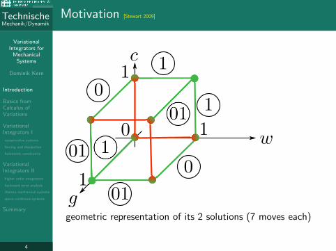
Crossing a river with a goat, a cabbage and a wolf..
VariationalIntegrators for
MechanicalSystems
Dominik Kern
Introduction
Basics fromCalculus ofVariations
VariationalIntegrators I
conservative systems
forcing and dissipation
holonomic constraints
VariationalIntegrators II
higher order integrators
backward error analysis
thermo-mechanical systems
space-continous systems
Summary
4
TechnischeMechanik/Dynamik
Motivation [Stewart 2009]
geometric representation of its 2 solutions (7 moves each)
VariationalIntegrators for
MechanicalSystems
Dominik Kern
Introduction
Basics fromCalculus ofVariations
VariationalIntegrators I
conservative systems
forcing and dissipation
holonomic constraints
VariationalIntegrators II
higher order integrators
backward error analysis
thermo-mechanical systems
space-continous systems
Summary
5
TechnischeMechanik/Dynamik
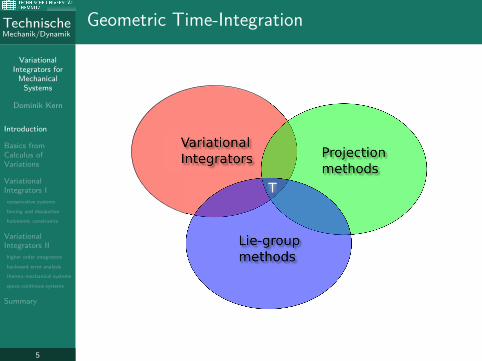
Geometric Time-Integration
VariationalIntegrators for
MechanicalSystems
Dominik Kern
Introduction
Basics fromCalculus ofVariations
VariationalIntegrators I
conservative systems
forcing and dissipation
holonomic constraints
VariationalIntegrators II
higher order integrators
backward error analysis
thermo-mechanical systems
space-continous systems
Summary
6
TechnischeMechanik/Dynamik
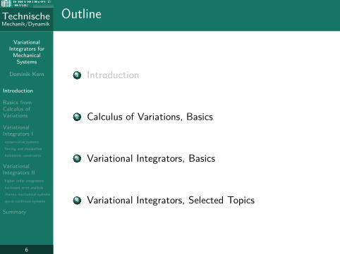
Outline
1 Introduction
2 Calculus of Variations, Basics
3 Variational Integrators, Basics
4 Variational Integrators, Selected Topics
VariationalIntegrators for
MechanicalSystems
Dominik Kern
Introduction
Basics fromCalculus ofVariations
VariationalIntegrators I
conservative systems
forcing and dissipation
holonomic constraints
VariationalIntegrators II
higher order integrators
backward error analysis
thermo-mechanical systems
space-continous systems
Summary
7
TechnischeMechanik/Dynamik
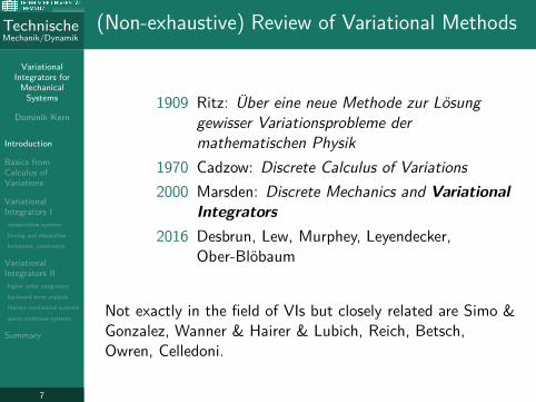
(Non-exhaustive) Review of Variational Methods
1909 Ritz: Über eine neue Methode zur Lösunggewisser Variationsprobleme dermathematischen Physik
1970 Cadzow: Discrete Calculus of Variations
2000 Marsden: Discrete Mechanics and Variational
Integrators
2016 Desbrun, Lew, Murphey, Leyendecker,Ober-Blöbaum
Not exactly in the field of VIs but closely related are Simo &Gonzalez, Wanner & Hairer & Lubich, Reich, Betsch,Owren, Celledoni.
VariationalIntegrators for
MechanicalSystems
Dominik Kern
Introduction
Basics fromCalculus ofVariations
VariationalIntegrators I
conservative systems
forcing and dissipation
holonomic constraints
VariationalIntegrators II
higher order integrators
backward error analysis
thermo-mechanical systems
space-continous systems
Summary
8
TechnischeMechanik/Dynamik
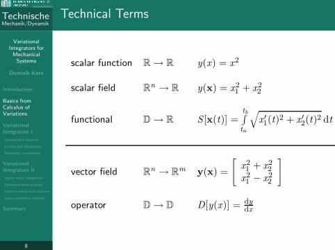
Technical Terms
scalar function R→ R y(x) = x2
scalar field Rn → R y(x) = x2
1 + x22
functional D→ R S [x(t)] =tb∫
ta
√
x ′1(t)2 + x ′2(t)2 dt
vector field Rn → R
m y(x) =
[
x21 + x2
2
x21 − x2
2
]
operator D→ D D[y(x)] = dydx
VariationalIntegrators for
MechanicalSystems
Dominik Kern
Introduction
Basics fromCalculus ofVariations
VariationalIntegrators I
conservative systems
forcing and dissipation
holonomic constraints
VariationalIntegrators II
higher order integrators
backward error analysis
thermo-mechanical systems
space-continous systems
Summary
9
TechnischeMechanik/Dynamik
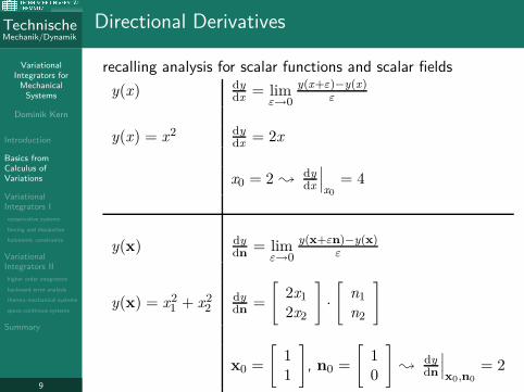
Directional Derivatives
recalling analysis for scalar functions and scalar fields
y(x) dydx
= limε→0
y(x+ε)−y(x)ε
y(x) = x2 dydx
= 2x
x0 = 2 ;dydx
∣∣∣x0
= 4
y(x) dydn
= limε→0
y(x+εn)−y(x)ε
y(x) = x21 + x2
2dydn
=
[
2x1
2x2
]
·
[
n1
n2
]
x0 =
[
11
]
, n0 =
[
10
]
;dydn
∣∣∣x0,n0
= 2
VariationalIntegrators for
MechanicalSystems
Dominik Kern
Introduction
Basics fromCalculus ofVariations
VariationalIntegrators I
conservative systems
forcing and dissipation
holonomic constraints
VariationalIntegrators II
higher order integrators
backward error analysis
thermo-mechanical systems
space-continous systems
Summary
10
TechnischeMechanik/Dynamik
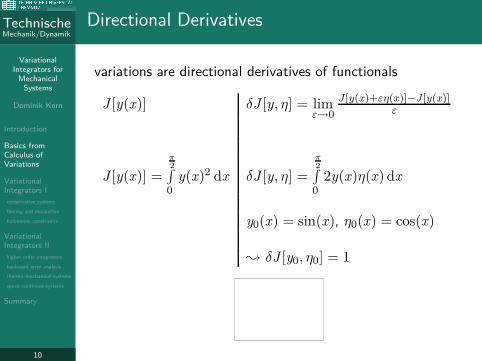
Directional Derivatives
variations are directional derivatives of functionals
J [y(x)] δJ [y, η] = limε→0
J [y(x)+εη(x)]−J [y(x)]ε
J [y(x)] =
π2∫
0y(x)2 dx δJ [y, η] =
π2∫
02y(x)η(x) dx
y0(x) = sin(x), η0(x) = cos(x)
; δJ [y0, η0] = 1
VariationalIntegrators for
MechanicalSystems
Dominik Kern
Introduction
Basics fromCalculus ofVariations
VariationalIntegrators I
conservative systems
forcing and dissipation
holonomic constraints
VariationalIntegrators II
higher order integrators
backward error analysis
thermo-mechanical systems
space-continous systems
Summary
11
TechnischeMechanik/Dynamik
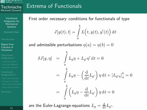
Extrema of Functionals
First order necessary conditions for functionals of type
J [y(t), t] =
b∫
a
L(
t, y(t), y′(t))
dt
and admissible perturbations η(a) = η(b) = 0
δJ [y, η] =
b∫
a
Lyη + Ly′η′ dt = 0
=
b∫
a
Lyη −
(d
dtLy′
)
η dt +∣∣Ly′η
∣∣b
a= 0
=
b∫
a
(
Lyη −d
dtLy′
)
η dt = 0
are the Euler-Lagrange-equations Ly = ddt
Ly′ .
VariationalIntegrators for
MechanicalSystems
Dominik Kern
Introduction
Basics fromCalculus ofVariations
VariationalIntegrators I
conservative systems
forcing and dissipation
holonomic constraints
VariationalIntegrators II
higher order integrators
backward error analysis
thermo-mechanical systems
space-continous systems
Summary
12
TechnischeMechanik/Dynamik
Extrema of Functionals
Remarks
There are a lot of applications in physics andengineering. The classical problems are Dido’s problem,Brachystochrone, Catenary, Geodetics, Minimalsurfaces, ...
The evaluation of sufficient conditions (of Legendre andJacobi) for extrema of functionals is more involved thanthose of functions and skipped here.
VariationalIntegrators for
MechanicalSystems
Dominik Kern
Introduction
Basics fromCalculus ofVariations
VariationalIntegrators I
conservative systems
forcing and dissipation
holonomic constraints
VariationalIntegrators II
higher order integrators
backward error analysis
thermo-mechanical systems
space-continous systems
Summary
13
TechnischeMechanik/Dynamik
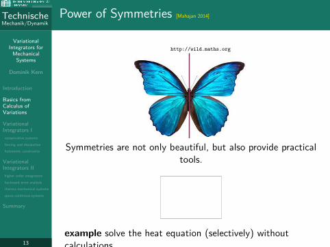
Power of Symmetries [Mahajan 2014]
http://wild.maths.org
Symmetries are not only beautiful, but also provide practicaltools.
example solve the heat equation (selectively) withoutcalculations.
VariationalIntegrators for
MechanicalSystems
Dominik Kern
Introduction
Basics fromCalculus ofVariations
VariationalIntegrators I
conservative systems
forcing and dissipation
holonomic constraints
VariationalIntegrators II
higher order integrators
backward error analysis
thermo-mechanical systems
space-continous systems
Summary
14
TechnischeMechanik/Dynamik
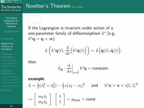
Noether’s Theorem [Levi 2014]
If the Lagrangian is invariant under action of aone-parameter family of diffeomorphism hs (e.g.hsq = q + se)
L
(
hsq(t),d
dt
(
hsq(t)))
= L(
q(t), q(t))
,
then
Lq ·d
ds
∣∣∣∣s=0
hsq = constant.
example
L = 12(x2
1 + x22 )− 1
2c(x2 − x1)2 and hsx = x + s[1, 1]T
;
[
m1x1
m2x2
]
·
[
11
]
= ptotal = const.
VariationalIntegrators for
MechanicalSystems
Dominik Kern
Introduction
Basics fromCalculus ofVariations
VariationalIntegrators I
conservative systems
forcing and dissipation
holonomic constraints
VariationalIntegrators II
higher order integrators
backward error analysis
thermo-mechanical systems
space-continous systems
Summary
15
TechnischeMechanik/Dynamik
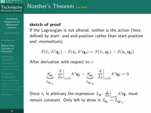
Noether’s Theorem [Levi 2014]
sketch of proof
If the Lagrangian is not altered, neither is the action (heredefined by start- and end-position rather than start-positionand -momentum)
S(t1, hsq1)− S(t0, h
sq0) = S(t1,q1)− S(t0,q0)
After derivation with respect to s
Sq1︸︷︷︸
Lq|t1
·d
ds
∣∣∣∣s=0
hsq1 − Sq0︸︷︷︸
Lq|t0
·d
ds
∣∣∣∣s=0
hsq0 = 0
Since t1 is arbitrary the expression Lq ·dds
∣∣∣s=0
hsq1 must
remain constant. Only left to show is Sq1= Lq|t1
.
VariationalIntegrators for
MechanicalSystems
Dominik Kern
Introduction
Basics fromCalculus ofVariations
VariationalIntegrators I
conservative systems
forcing and dissipation
holonomic constraints
VariationalIntegrators II
higher order integrators
backward error analysis
thermo-mechanical systems
space-continous systems
Summary
16
TechnischeMechanik/Dynamik
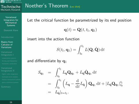
Noether’s Theorem [Levi 2014]
Let the critical function be parametrized by its end position
q(t) = Q(t, t1,q1)
insert into the action function
S(t1,q1) =
∫ t1
t0
L(Q, Q) dt
and differentiate by q1
Sq1=
∫ t1
t0
LqQq1+ LqQq1
dt
=
∫ t1
t0
(
Lq −d
dtLq
)
Qq1dt + |LqQq1
|t1
t0
= Lq|t=t1.
VariationalIntegrators for
MechanicalSystems
Dominik Kern
Introduction
Basics fromCalculus ofVariations
VariationalIntegrators I
conservative systems
forcing and dissipation
holonomic constraints
VariationalIntegrators II
higher order integrators
backward error analysis
thermo-mechanical systems
space-continous systems
Summary
17
TechnischeMechanik/Dynamik
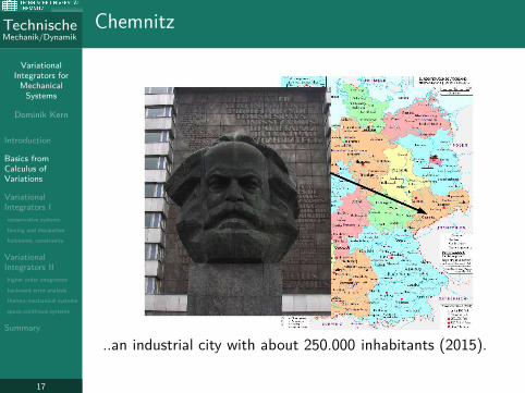
Chemnitz
..an industrial city with about 250.000 inhabitants (2015).
VariationalIntegrators for
MechanicalSystems
Dominik Kern
Introduction
Basics fromCalculus ofVariations
VariationalIntegrators I
conservative systems
forcing and dissipation
holonomic constraints
VariationalIntegrators II
higher order integrators
backward error analysis
thermo-mechanical systems
space-continous systems
Summary
18
TechnischeMechanik/Dynamik
Point of Departure
Hamilton’s principle rules the classical mechanics
δ
te∫
tb
L(q, q) dt = 0 with L = T (q, q)− V (q),
typically used for equations of motion
d
dt
(∂L
∂q
)
−∂L
∂q= 0,
which are often nonlinear and solved numerically.
The Lagrangian L(q, q) lives on tangent bundleL : TM → R of the configuration manifold M .
VariationalIntegrators for
MechanicalSystems
Dominik Kern
Introduction
Basics fromCalculus ofVariations
VariationalIntegrators I
conservative systems
forcing and dissipation
holonomic constraints
VariationalIntegrators II
higher order integrators
backward error analysis
thermo-mechanical systems
space-continous systems
Summary
19
TechnischeMechanik/Dynamik
Point of Departure
Equivalently, the system can be brought into Hamiltonianform by the Legendre Transformation
H (q,p) = p · q − L.
Due to substitution of variables, presuming ∂2L∂q∂q
regular
p(q, q) =∂L
∂q.
The Hamiltonian H (q,p) lives on co-tangent bundleH : T ∗M → R of the configuration manifold M .
The equations of motions then become
[
q
p
]
=
[
0 1−1 0
] [∂H∂q∂H∂p
]
.
VariationalIntegrators for
MechanicalSystems
Dominik Kern
Introduction
Basics fromCalculus ofVariations
VariationalIntegrators I
conservative systems
forcing and dissipation
holonomic constraints
VariationalIntegrators II
higher order integrators
backward error analysis
thermo-mechanical systems
space-continous systems
Summary
20
TechnischeMechanik/Dynamik
Point of Departure
For the simple pendulum
L =1
2ϕ2 + cosϕ
the equations of motion are either (Lagrangian form)
ϕ+ sinϕ = 0,
with ϕ(0) = ϕ0, ϕ(0) = ϕ0, or (Hamiltonian form)
ϕ = p
p = − sinϕ
with ϕ(0) = ϕ0 p(0) = p0.
VariationalIntegrators for
MechanicalSystems
Dominik Kern
Introduction
Basics fromCalculus ofVariations
VariationalIntegrators I
conservative systems
forcing and dissipation
holonomic constraints
VariationalIntegrators II
higher order integrators
backward error analysis
thermo-mechanical systems
space-continous systems
Summary
21
TechnischeMechanik/Dynamik
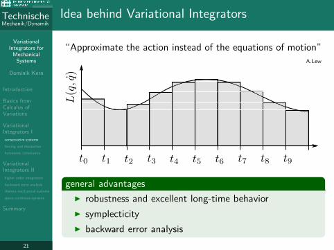
Idea behind Variational Integrators
“Approximate the action instead of the equations of motion”A.Lew
general advantages
robustness and excellent long-time behavior
symplecticity
backward error analysis
VariationalIntegrators for
MechanicalSystems
Dominik Kern
Introduction
Basics fromCalculus ofVariations
VariationalIntegrators I
conservative systems
forcing and dissipation
holonomic constraints
VariationalIntegrators II
higher order integrators
backward error analysis
thermo-mechanical systems
space-continous systems
Summary
22
TechnischeMechanik/Dynamik
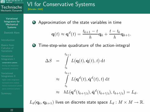
VI for Conservative Systems[Marsden 2000]
1 Approximation of the state variables in time
q(t) ≈ qd(t) =tk+1 − t
hqk +
t − tk
hqk+1.
2 Time-step-wise quadrature of the action-integral
∆S =
tk+1∫
tk
L(q(t), q(t), t
)dt
≈
tk+1∫
tk
L(qd(t), qd(t), t
)dt
≈ hL(
qd(tk+1/2), qd(tk+1/2), tk+1/2
)
= Ld .
Ld(qk ,qk+1) lives on discrete state space Ld : M ×M → R.
VariationalIntegrators for
MechanicalSystems
Dominik Kern
Introduction
Basics fromCalculus ofVariations
VariationalIntegrators I
conservative systems
forcing and dissipation
holonomic constraints
VariationalIntegrators II
higher order integrators
backward error analysis
thermo-mechanical systems
space-continous systems
Summary
23
TechnischeMechanik/Dynamik
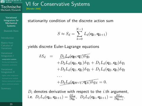
VI for Conservative Systems[Marsden 2000]
stationarity condition of the discrete action sum
S ≈ Sd =N−1∑
k=0
Ld(qk ,qk+1)
yields discrete Euler-Lagrange equations
δSd =(
((
((
((
(
D1Ld(q0,q1)δq0
+D2Ld(q0,q1)δq1 + D1Ld(q1,q2)δq1
+D2Ld(q1,q2)δq2 + D1Ld(q2,q3)δq2
. . .
+(
((
((
((
((
(
D2Ld(qN−1,qN )δqN = 0.
Di denotes derivative with respect to the i.th argument,i.e. D1Ld(qk ,qk+1) = ∂Ld
∂qk, D2Ld(qk ,qk+1) = ∂Ld
∂qk+1.
VariationalIntegrators for
MechanicalSystems
Dominik Kern
Introduction
Basics fromCalculus ofVariations
VariationalIntegrators I
conservative systems
forcing and dissipation
holonomic constraints
VariationalIntegrators II
higher order integrators
backward error analysis
thermo-mechanical systems
space-continous systems
Summary
24
TechnischeMechanik/Dynamik
VI for Conservative Systems[Marsden 2000]
The DEL determine qk , qk−1 ; qk+1 implicitly by
D2Ld(qk−1,qk) + D1Ld(qk ,qk+1) = 0.
On one hand the I.C. q0, q0 correspond to the momenta
p0 =∂L
∂q
∣∣∣∣q0,q0
on the other hand the velocity approximation corresponds to
p1/2 =∂L
∂q
∣∣∣∣q1/2,q1/2
correction by the acting forces between t0 . . . t0 + h/2
p0 = D2L(q0, q) = −D1Ld(q0,q1) = p1/2 −h
2
∂L
∂q
∣∣∣∣q1/2
to be detailed later (discrete Legendre Transform).
VariationalIntegrators for
MechanicalSystems
Dominik Kern
Introduction
Basics fromCalculus ofVariations
VariationalIntegrators I
conservative systems
forcing and dissipation
holonomic constraints
VariationalIntegrators II
higher order integrators
backward error analysis
thermo-mechanical systems
space-continous systems
Summary
25
TechnischeMechanik/Dynamik
Example
1DoF system (dimensionless), e.g. simple pendulum
L =1
2q2 − V (q)
with linear approximations for the time step t = 0 . . . h
q ≈ qd =h − t
hq0 +
t
hq1 and q ≈ qd =
q1 − q0
h
and trapezoidal rule for quadrature
∫ h
0L(qd , qd) ≈
h
2L(q0, q
d)
+h
2L(q1, q
d)
= Ld
results in the popular Störmer-Verlet scheme [Verlet1967].
δSd = 0 ;
p0 = qd + h2∂V∂q
(q0) ; q1
p1 = qd − h2∂V∂q
(q1) ; p1
VariationalIntegrators for
MechanicalSystems
Dominik Kern
Introduction
Basics fromCalculus ofVariations
VariationalIntegrators I
conservative systems
forcing and dissipation
holonomic constraints
VariationalIntegrators II
higher order integrators
backward error analysis
thermo-mechanical systems
space-continous systems
Summary
26
TechnischeMechanik/Dynamik
Symplecticity[Arnold 1974]
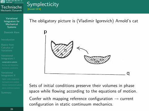
The obligatory picture is (Vladimir Igorevich) Arnold’s cat
Sets of initial conditions preserve their volumes in phasespace while flowing according to the equations of motion.
Confer with mapping reference configuration → currentconfiguration in static continuum mechanics.
VariationalIntegrators for
MechanicalSystems
Dominik Kern
Introduction
Basics fromCalculus ofVariations
VariationalIntegrators I
conservative systems
forcing and dissipation
holonomic constraints
VariationalIntegrators II
higher order integrators
backward error analysis
thermo-mechanical systems
space-continous systems
Summary
27
TechnischeMechanik/Dynamik
Symplecticity
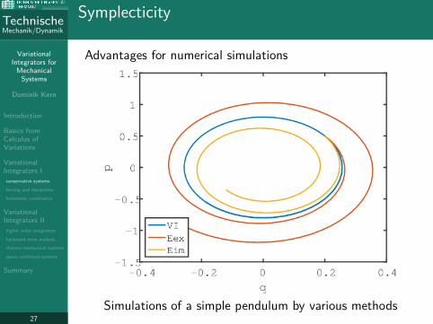
Advantages for numerical simulations
Simulations of a simple pendulum by various methods
VariationalIntegrators for
MechanicalSystems
Dominik Kern
Introduction
Basics fromCalculus ofVariations
VariationalIntegrators I
conservative systems
forcing and dissipation
holonomic constraints
VariationalIntegrators II
higher order integrators
backward error analysis
thermo-mechanical systems
space-continous systems
Summary
28
TechnischeMechanik/Dynamik
Discrete Legendre Transform[Lew 2004]
Similarly to the continous case, there is a discretemomentum definition.
pk = −D1Ld(qk ,qk+1)
pk+1 = D2Ld(qk ,qk+1)
whose continuity is enforced by the DEL.
Hint, express derived quantities, such as velocities orenergies, as functions of qk and pk , instead of evaluating the
approximations qd(t)!
VariationalIntegrators for
MechanicalSystems
Dominik Kern
Introduction
Basics fromCalculus ofVariations
VariationalIntegrators I
conservative systems
forcing and dissipation
holonomic constraints
VariationalIntegrators II
higher order integrators
backward error analysis
thermo-mechanical systems
space-continous systems
Summary
29
TechnischeMechanik/Dynamik
Discrete Noether Theorem
If there is a one-parameter group hs that leaves
Ld(hsqk , hsqk+1) = Ld(qk ,qk+1)
invariant, then there is an invariant of the dynamics
I (qk ,pk) = pk ·d
dshsqk = constant.
example: two masses connected by a spring
L = 12m(x2 + y2)− 1
2c(y − x)2, hsq = q + [s, s]T
p0 = −D1Ld =
[
m x1−x0
h− h
2 c(y1/2 − x1/2)
m y1−y0
h+ h
2 c(y1/2 − x1/2)
]
p1 = D2Ld =
[
m x1−x0
h+ h
2 c(y1/2 − x1/2)
m y1−y0
h− h
2 c(y1/2 − x1/2)
]
I = mx1 − x0
h+ m
y1 − y0
h
VariationalIntegrators for
MechanicalSystems
Dominik Kern
Introduction
Basics fromCalculus ofVariations
VariationalIntegrators I
conservative systems
forcing and dissipation
holonomic constraints
VariationalIntegrators II
higher order integrators
backward error analysis
thermo-mechanical systems
space-continous systems
Summary
30
TechnischeMechanik/Dynamik
Forcing and Dissipation[Marsden 2000]
Discrete Lagrange-D’Alembert principle, derived fromtime-continous formulation
δ
te∫
tb
L dt +
te∫
tb
δW nc dt =N−1∑
k=0
δ
tk+1∫
tk
L dt + +
tk+1∫
tk
δW nc dt = 0
L as before and virtual work of non-conservative forces by
tk+1∫
tk
δW nc dt =
tk+1∫
tk
F(t) · δq(t) dt ≈
tk+1∫
tk
F(t) · δqd(t) dt
≈ hF(tk+1/2) · δqd(tk+1/2) = F−k δqk + F+
k+1δqk+1.
DEL arranged in position-momentum form
pk = −D1Ld(qk ,qk+1)− F−k (qk ,qk+1)
pk+1 = D2Ld(qk ,qk+1) + F+k (qk ,qk+1).
VariationalIntegrators for
MechanicalSystems
Dominik Kern
Introduction
Basics fromCalculus ofVariations
VariationalIntegrators I
conservative systems
forcing and dissipation
holonomic constraints
VariationalIntegrators II
higher order integrators
backward error analysis
thermo-mechanical systems
space-continous systems
Summary
31
TechnischeMechanik/Dynamik
Alternative Approach[Vujanovic 1988]
For linear systems with damping
x + 2Dx + ω20x = 0
L =1
2(x2 − ω2
0x2)e2Dt ,
or forcing
x + ω20x = a cos Ωt
L =1
2
(
x +aΩ sin Ωt
ω20 − Ω2
)2
−ω2
0
2
(
x −a cos Ωt
ω20 − Ω2
)2
.
Generally seems the inverse problem of the calculus ofvariations to be an interesting approach.
VariationalIntegrators for
MechanicalSystems
Dominik Kern
Introduction
Basics fromCalculus ofVariations
VariationalIntegrators I
conservative systems
forcing and dissipation
holonomic constraints
VariationalIntegrators II
higher order integrators
backward error analysis
thermo-mechanical systems
space-continous systems
Summary
32
TechnischeMechanik/Dynamik
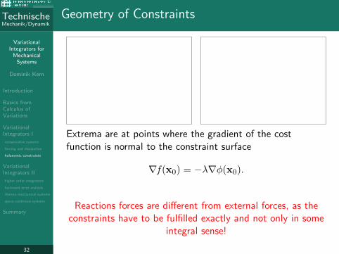
Geometry of Constraints
Extrema are at points where the gradient of the costfunction is normal to the constraint surface
∇f (x0) = −λ∇φ(x0).
Reactions forces are different from external forces, as theconstraints have to be fulfilled exactly and not only in some
integral sense!
VariationalIntegrators for
MechanicalSystems
Dominik Kern
Introduction
Basics fromCalculus ofVariations
VariationalIntegrators I
conservative systems
forcing and dissipation
holonomic constraints
VariationalIntegrators II
higher order integrators
backward error analysis
thermo-mechanical systems
space-continous systems
Summary
33
TechnischeMechanik/Dynamik
VI for Constrained Systems[Marsden 2000]
Basically it works to enforce the constraints on position levelonly, better is enforcement on position and momentum level.
Iteration equations enforce constraint φ = 0
0 = pk + D1Ld(qk ,qk+1)− λk∇φ(qk)
0 = φ(qk+1),
while update-equations enforce “hidden” constraint (φ = 0)
pk+1 = D2Ld(qk ,qk+1)− λk+1∇φ(qk+1)
0 = ∇φ(qk+1) ·∂H
∂p(qk+1,pk+1).
Alternatively, eliminate the Lagrange-multipliers by thenullspace method [Betsch2005], for VI [Leyendecker2008].
VariationalIntegrators for
MechanicalSystems
Dominik Kern
Introduction
Basics fromCalculus ofVariations
VariationalIntegrators I
conservative systems
forcing and dissipation
holonomic constraints
VariationalIntegrators II
higher order integrators
backward error analysis
thermo-mechanical systems
space-continous systems
Summary
34
TechnischeMechanik/Dynamik
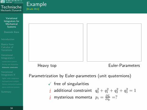
Example[Bruels 2011]
Heavy top Euler-Parameters
Parametrization by Euler-parameters (unit quaternions)
X free of singularities
additional constraint q20 + q2
1 + q22 + q2
3 = 1
mysterious momenta pi = ∂L∂qi
=?
VariationalIntegrators for
MechanicalSystems
Dominik Kern
Introduction
Basics fromCalculus ofVariations
VariationalIntegrators I
conservative systems
forcing and dissipation
holonomic constraints
VariationalIntegrators II
higher order integrators
backward error analysis
thermo-mechanical systems
space-continous systems
Summary
35
TechnischeMechanik/Dynamik
Example[Betsch 2006]
Crucial point ist the kinetic energy
T =1
2q ·M4q,
with the rank-one augmented mass matrix
M4 = 4G(q)T JG(q) + 2tr(J)q ⊗ q,
where G(q) relates to the convective angular velocity
Ω = 2G(q)q q =1
2G(q)T Ω.
Potential energy as usual
V = mgez · xs = mgez ·R(q)Xs.
VariationalIntegrators for
MechanicalSystems
Dominik Kern
Introduction
Basics fromCalculus ofVariations
VariationalIntegrators I
conservative systems
forcing and dissipation
holonomic constraints
VariationalIntegrators II
higher order integrators
backward error analysis
thermo-mechanical systems
space-continous systems
Summary
36
TechnischeMechanik/Dynamik
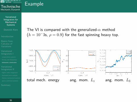
Example
The VI is compared with the generalized-α method(h = 10−3s, ρ = 0.9) for the fast spinning heavy top.
total mech. energy ang. mom. Lz ang. mom. L3
VariationalIntegrators for
MechanicalSystems
Dominik Kern
Introduction
Basics fromCalculus ofVariations
VariationalIntegrators I
conservative systems
forcing and dissipation
holonomic constraints
VariationalIntegrators II
higher order integrators
backward error analysis
thermo-mechanical systems
space-continous systems
Summary
37
TechnischeMechanik/Dynamik
TU Chemnitz
www.panoramio.com
.. a technical university with about 11.000 students (2015).
VariationalIntegrators for
MechanicalSystems
Dominik Kern
Introduction
Basics fromCalculus ofVariations
VariationalIntegrators I
conservative systems
forcing and dissipation
holonomic constraints
VariationalIntegrators II
higher order integrators
backward error analysis
thermo-mechanical systems
space-continous systems
Summary
38
TechnischeMechanik/Dynamik
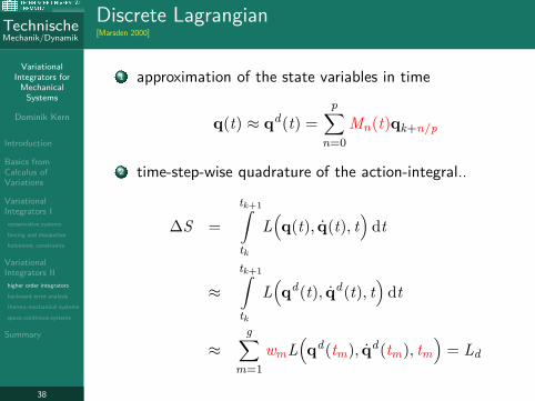
Discrete Lagrangian[Marsden 2000]
1 approximation of the state variables in time
q(t) ≈ qd(t) =p∑
n=0
Mn(t)qk+n/p
2 time-step-wise quadrature of the action-integral..
∆S =
tk+1∫
tk
L(
q(t), q(t), t)
dt
≈
tk+1∫
tk
L(
qd(t), qd(t), t)
dt
≈g∑
m=1
wmL(
qd(tm), qd(tm), tm
)
= Ld
VariationalIntegrators for
MechanicalSystems
Dominik Kern
Introduction
Basics fromCalculus ofVariations
VariationalIntegrators I
conservative systems
forcing and dissipation
holonomic constraints
VariationalIntegrators II
higher order integrators
backward error analysis
thermo-mechanical systems
space-continous systems
Summary
39
TechnischeMechanik/Dynamik
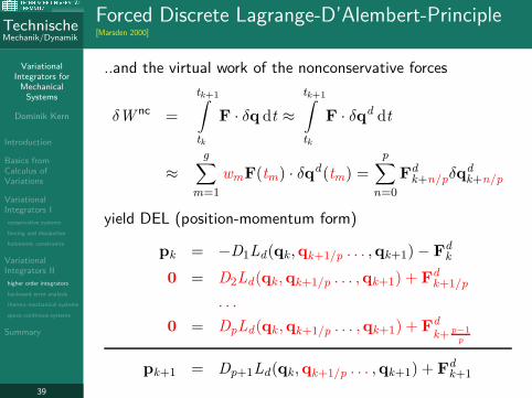
Forced Discrete Lagrange-D’Alembert-Principle[Marsden 2000]
..and the virtual work of the nonconservative forces
δW nc =
tk+1∫
tk
F · δq dt ≈
tk+1∫
tk
F · δqd dt
≈g∑
m=1
wmF(tm) · δqd(tm) =p∑
n=0
Fdk+n/pδq
dk+n/p
yield DEL (position-momentum form)
pk = −D1Ld(qk ,qk+1/p . . . ,qk+1)− Fdk
0 = D2Ld(qk ,qk+1/p . . . ,qk+1) + Fdk+1/p
. . .
0 = DpLd(qk ,qk+1/p . . . ,qk+1) + Fd
k+ p−1
p
pk+1 = Dp+1Ld(qk ,qk+1/p . . . ,qk+1) + Fdk+1
VariationalIntegrators for
MechanicalSystems
Dominik Kern
Introduction
Basics fromCalculus ofVariations
VariationalIntegrators I
conservative systems
forcing and dissipation
holonomic constraints
VariationalIntegrators II
higher order integrators
backward error analysis
thermo-mechanical systems
space-continous systems
Summary
40
TechnischeMechanik/Dynamik
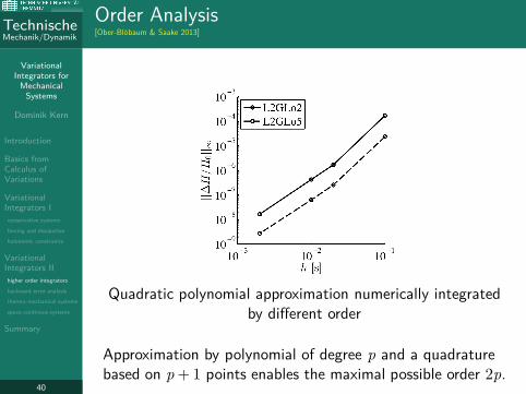
Order Analysis[Ober-Blöbaum & Saake 2013]
Quadratic polynomial approximation numerically integratedby different order
Approximation by polynomial of degree p and a quadraturebased on p + 1 points enables the maximal possible order 2p.
VariationalIntegrators for
MechanicalSystems
Dominik Kern
Introduction
Basics fromCalculus ofVariations
VariationalIntegrators I
conservative systems
forcing and dissipation
holonomic constraints
VariationalIntegrators II
higher order integrators
backward error analysis
thermo-mechanical systems
space-continous systems
Summary
41
TechnischeMechanik/Dynamik
Backward Error Analysis[Hairer & Wanner & Lubich 2006]
Rather than considering how closely the approximatedtrajectories match the exact ones, it is now considered howclosely the discrete Lagrangian (Hamiltonian) matches theideal one.
Backward error analysis reveals discrete time paths as exactsolutions of a nearby Hamiltonian
H (q, p) = H (q, p) + hg1(q, p) + h2g2(q, p) + . . .
VariationalIntegrators for
MechanicalSystems
Dominik Kern
Introduction
Basics fromCalculus ofVariations
VariationalIntegrators I
conservative systems
forcing and dissipation
holonomic constraints
VariationalIntegrators II
higher order integrators
backward error analysis
thermo-mechanical systems
space-continous systems
Summary
42
TechnischeMechanik/Dynamik
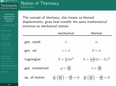
Notion of Thermacy[Helmholtz 1884]
The concept of thermacy, also known as thermaldisplacements, gives heat transfer the same mathematicalstructure as mechanical motion.
mechanical thermal
gen. coord. x α
gen. vel. v = x ϑ = α
Lagrangian L = 12mx2 L = 1
2kϑr
(α − ϑr)2
gen. momentum p = ∂L∂x
s = ∂L∂α
eq. of motion ddt
(∂L∂x
)
− ∂L∂x
= 0 ddt
(∂L∂α
)
− ∂L∂α = 0
VariationalIntegrators for
MechanicalSystems
Dominik Kern
Introduction
Basics fromCalculus ofVariations
VariationalIntegrators I
conservative systems
forcing and dissipation
holonomic constraints
VariationalIntegrators II
higher order integrators
backward error analysis
thermo-mechanical systems
space-continous systems
Summary
43
TechnischeMechanik/Dynamik
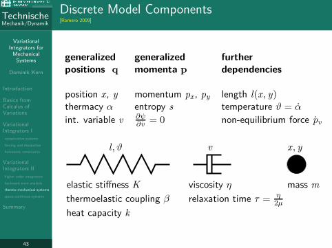
Discrete Model Components[Romero 2009]
generalized generalized further
positions q momenta p dependencies
position x, y momentum px , py length l(x, y)thermacy α entropy s temperature ϑ = α
int. variable v ∂ψ∂v
= 0 non-equilibrium force pv
l, ϑ
elastic stiffness K
thermoelastic coupling β
heat capacity k
v
viscosity η
relaxation time τ = η2µ
x, y
mass m
VariationalIntegrators for
MechanicalSystems
Dominik Kern
Introduction
Basics fromCalculus ofVariations
VariationalIntegrators I
conservative systems
forcing and dissipation
holonomic constraints
VariationalIntegrators II
higher order integrators
backward error analysis
thermo-mechanical systems
space-continous systems
Summary
44
TechnischeMechanik/Dynamik
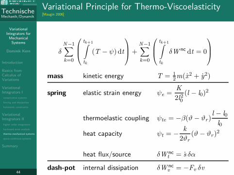
Variational Principle for Thermo-Viscoelasticity[Maugin 2006]
δN−1∑
k=0
tk+1∫
tk
(T − ψ) dt
+
N−1∑
k=0
tk+1∫
tk
δW nc dt = 0
mass kinetic energy T = 12m(x2 + y2)
spring elastic strain energy ψe =K
2l20
(l − l0)2
thermoelastic coupling ψte = −β(ϑ − ϑr)l − l0
l0
heat capacity ψt = −k
2ϑr
(ϑ − ϑr)2
heat flux/source δW nct = s δα
dash-pot internal dissipation δW ncv = −Fv δv
VariationalIntegrators for
MechanicalSystems
Dominik Kern
Introduction
Basics fromCalculus ofVariations
VariationalIntegrators I
conservative systems
forcing and dissipation
holonomic constraints
VariationalIntegrators II
higher order integrators
backward error analysis
thermo-mechanical systems
space-continous systems
Summary
45
TechnischeMechanik/Dynamik
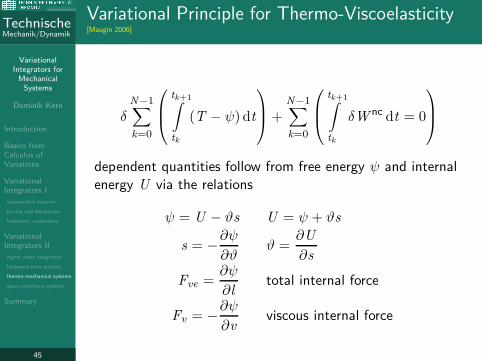
Variational Principle for Thermo-Viscoelasticity[Maugin 2006]
δN−1∑
k=0
tk+1∫
tk
(T − ψ) dt
+
N−1∑
k=0
tk+1∫
tk
δW nc dt = 0
dependent quantities follow from free energy ψ and internalenergy U via the relations
ψ = U − ϑs U = ψ + ϑs
s = −∂ψ
∂ϑϑ =
∂U
∂s
Fve =∂ψ
∂ltotal internal force
Fv = −∂ψ
∂vviscous internal force
VariationalIntegrators for
MechanicalSystems
Dominik Kern
Introduction
Basics fromCalculus ofVariations
VariationalIntegrators I
conservative systems
forcing and dissipation
holonomic constraints
VariationalIntegrators II
higher order integrators
backward error analysis
thermo-mechanical systems
space-continous systems
Summary
46
TechnischeMechanik/Dynamik
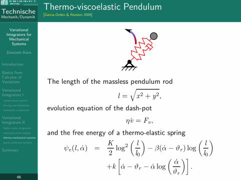
Thermo-viscoelastic Pendulum[Garcia-Orden & Romero 2006]
The length of the massless pendulum rod
l =√
x2 + y2,
evolution equation of the dash-pot
ηv = Fv ,
and the free energy of a thermo-elastic spring
ψe(l, α) =K
2log2
(l
l0
)
− β(α − ϑr) log
(l
l0
)
+k
[
α− ϑr − α log
(α
ϑr
)]
.
VariationalIntegrators for
MechanicalSystems
Dominik Kern
Introduction
Basics fromCalculus ofVariations
VariationalIntegrators I
conservative systems
forcing and dissipation
holonomic constraints
VariationalIntegrators II
higher order integrators
backward error analysis
thermo-mechanical systems
space-continous systems
Summary
47
TechnischeMechanik/Dynamik
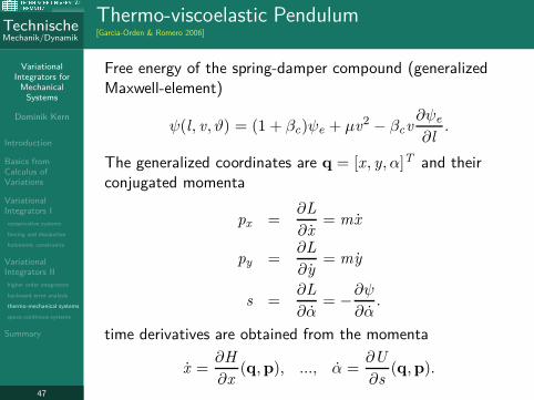
Thermo-viscoelastic Pendulum[Garcia-Orden & Romero 2006]
Free energy of the spring-damper compound (generalizedMaxwell-element)
ψ(l, v, ϑ) = (1 + βc)ψe + µv2 − βcv∂ψe
∂l.
The generalized coordinates are q = [x, y, α]T and theirconjugated momenta
px =∂L
∂x= mx
py =∂L
∂y= my
s =∂L
∂α= −
∂ψ
∂α.
time derivatives are obtained from the momenta
x =∂H
∂x(q,p), ..., α =
∂U
∂s(q,p).
VariationalIntegrators for
MechanicalSystems
Dominik Kern
Introduction
Basics fromCalculus ofVariations
VariationalIntegrators I
conservative systems
forcing and dissipation
holonomic constraints
VariationalIntegrators II
higher order integrators
backward error analysis
thermo-mechanical systems
space-continous systems
Summary
48
TechnischeMechanik/Dynamik
Thermo-viscoelastic Pendulum[Garcia-Orden & Romero 2006]
Heat transfer (Fourier type, thermal conductivity κ) betweenspring and environment
h = −κ(α− ϑ∞).
Regarding the dash-pot, it is assumed that all energymechanically dissipated is completely converted into heat,which corresponds to the entropy production
sv =gv
α.
Adding the mechanical dissipation up to the previous twoeffects
δW nc = −Fvδv +Fv v
αδα− κ
α− ϑ∞α
δα.
VariationalIntegrators for
MechanicalSystems
Dominik Kern
Introduction
Basics fromCalculus ofVariations
VariationalIntegrators I
conservative systems
forcing and dissipation
holonomic constraints
VariationalIntegrators II
higher order integrators
backward error analysis
thermo-mechanical systems
space-continous systems
Summary
49
TechnischeMechanik/Dynamik
Thermo-viscoelastic Pendulum[Garcia-Orden & Romero 2006]
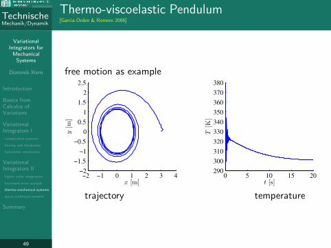
free motion as example
−2 −1 0 1 2 3 4−2
−1.5
−1
−0.5
0
0.5
1
1.5
2
2.5
y[m
]
x [m]0 5 10 15 20
290
300
310
320
330
340
350
360
370
380
T[K
]
t [s]
trajectory temperature
VariationalIntegrators for
MechanicalSystems
Dominik Kern
Introduction
Basics fromCalculus ofVariations
VariationalIntegrators I
conservative systems
forcing and dissipation
holonomic constraints
VariationalIntegrators II
higher order integrators
backward error analysis
thermo-mechanical systems
space-continous systems
Summary
50
TechnischeMechanik/Dynamik
Thermo-viscoelastic Pendulum[Garcia-Orden & Romero 2006]
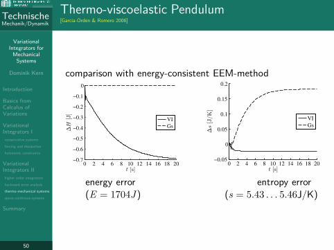
comparison with energy-consistent EEM-method
0 2 4 6 8 10 12 14 16 18 20−0.7
−0.6
−0.5
−0.4
−0.3
−0.2
−0.1
0
t [s]
∆H
[J]
VI
Gs
0 2 4 6 8 10 12 14 16 18 20−0.05
0
0.05
0.1
0.15
0.2
t [s]
∆s[J/K]
VI
Gs
energy error entropy error(E = 1704J ) (s = 5.43 . . . 5.46J/K)
VariationalIntegrators for
MechanicalSystems
Dominik Kern
Introduction
Basics fromCalculus ofVariations
VariationalIntegrators I
conservative systems
forcing and dissipation
holonomic constraints
VariationalIntegrators II
higher order integrators
backward error analysis
thermo-mechanical systems
space-continous systems
Summary
51
TechnischeMechanik/Dynamik
Non-standard Heat Transfer[Green & Naghdi 1991]
For Green & Naghdi type II heat transfer simply add
ψGN2 =1
2κII|∇α|
2
to the free energy.
+ Hamiltonian structure fits perfectly inVI-framework [Mata & Lew 2013]
- low practical relevance
- open questions
VariationalIntegrators for
MechanicalSystems
Dominik Kern
Introduction
Basics fromCalculus ofVariations
VariationalIntegrators I
conservative systems
forcing and dissipation
holonomic constraints
VariationalIntegrators II
higher order integrators
backward error analysis
thermo-mechanical systems
space-continous systems
Summary
52
TechnischeMechanik/Dynamik
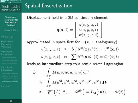
Spatial Discretization
Displacement field in a 3D-continuum element
q(x, t) =
u(x, y, z, t)v(x, y, z, t)w(x, y, z, t)
approximated in space first for u (v, w analogously)
u(x, y, z, t) ≈∑
N n(x)un(t) = usd(x, t)
u(x, y, z, t) ≈∑
N n(x)un(t) = usd(x, t)
leads as intermediate step to a semidiscrete Lagrangian
L =
∫
VL(u, v,w, u, v, w) dV
≈
∫
VL(usd, vsd,wsd, usd, vsd, wsd) dV
≈ InumV
(
L(usd, . . . , wsd))
= Lsd
(
u(t), . . . , w(t))
.
VariationalIntegrators for
MechanicalSystems
Dominik Kern
Introduction
Basics fromCalculus ofVariations
VariationalIntegrators I
conservative systems
forcing and dissipation
holonomic constraints
VariationalIntegrators II
higher order integrators
backward error analysis
thermo-mechanical systems
space-continous systems
Summary
53
TechnischeMechanik/Dynamik
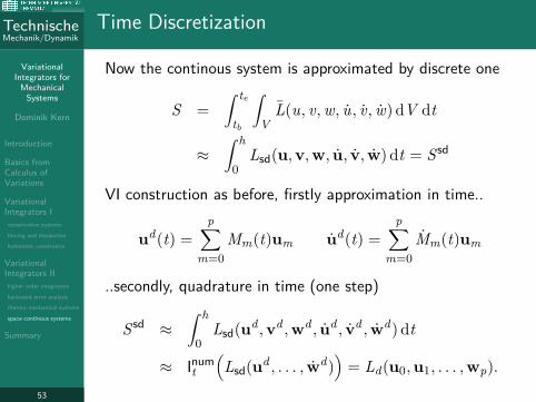
Time Discretization
Now the continous system is approximated by discrete one
S =
∫ te
tb
∫
VL(u, v,w, u, v, w) dV dt
≈
∫ h
0Lsd(u,v,w, u, v, w) dt = S sd
VI construction as before, firstly approximation in time..
ud(t) =p∑
m=0
Mm(t)um ud(t) =p∑
m=0
Mm(t)um
..secondly, quadrature in time (one step)
S sd ≈
∫ h
0Lsd(ud ,vd ,wd , ud , vd , wd) dt
≈ Inumt
(
Lsd(ud , . . . , wd))
= Ld(u0,u1, . . . ,wp).
VariationalIntegrators for
MechanicalSystems
Dominik Kern
Introduction
Basics fromCalculus ofVariations
VariationalIntegrators I
conservative systems
forcing and dissipation
holonomic constraints
VariationalIntegrators II
higher order integrators
backward error analysis
thermo-mechanical systems
space-continous systems
Summary
54
TechnischeMechanik/Dynamik
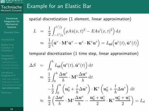
Example for an Elastic Bar
spatial discretization (1 element, linear approximation)
L =1
2
∫ Le/2
−Le/2
(
Au(x, t)2 − EAu′(x, t)2)
dx
≈1
2
(
ue ·Meue − ue ·Keue)
= Lsd
(
ue(t), ue(t))
temporal discretization (1 time step, linear approximation)
∆S =
∫ h
0Lsd
(
ue(t), ue(t))
dt
≈1
2
∫ h
0
∆ue
h·Me ∆ue
hdt
−1
2
∫ h
0
(
ue0 +
t
h∆ue
)
·Ke
(
ue0 +
t
h∆ue
)
dt
≈h
2
(∆ue
h·Me ∆ue
h−
ue0 + ue
1
2·Ke ue
0 + ue1
2
)
= Ld
VariationalIntegrators for
MechanicalSystems
Dominik Kern
Introduction
Basics fromCalculus ofVariations
VariationalIntegrators I
conservative systems
forcing and dissipation
holonomic constraints
VariationalIntegrators II
higher order integrators
backward error analysis
thermo-mechanical systems
space-continous systems
Summary
55
TechnischeMechanik/Dynamik
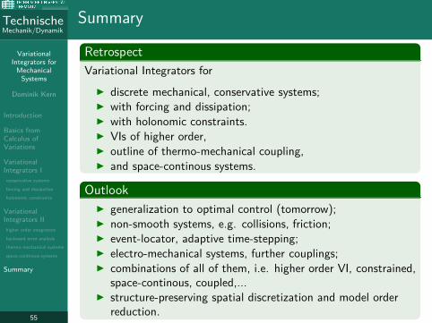
Summary
Retrospect
Variational Integrators for
discrete mechanical, conservative systems; with forcing and dissipation; with holonomic constraints. VIs of higher order, outline of thermo-mechanical coupling, and space-continous systems.
Outlook
generalization to optimal control (tomorrow); non-smooth systems, e.g. collisions, friction; event-locator, adaptive time-stepping; electro-mechanical systems, further couplings; combinations of all of them, i.e. higher order VI, constrained,
space-continous, coupled,... structure-preserving spatial discretization and model order
reduction.
Recommended