Download pdf - Unit1.Inner Product Spaces

Unit 5Inner Product Spaces and OrthogonalVectors

5.1 IntroductionIn previous units we have looked at general vector spaces defined by a very small number of definingaxioms, and have looked at many specific examples of such vector spaces. However, in our usual viewof the space in which we live we always think of it having certain properties such as distance andangles that do not occur in many vector spaces. In this Unit we investigate vector spaces that have oneadditional property, an inner product, that allows us to define distance, angle and other properties andwe call these inner product spaces. We have already studied some special cases of these in theEuclidean Vector Spaces,, Rn, for n = 1, 2, · · · , but in this unit we show how the same results apply toother vector spaces. In particular the Euclidean space aspect is covered in the subsection ”Geometryof Linear Transformations Between R2, R3 and R” of Unit 3, Section 3: Linear Transformations from Rn

to Rm.

The approach in this section follows a very important and powerful mathematical approach in which avery general concept, such as inner product spaces, is developed from only a very few basic definingproperties, or axioms. The properties developed for the general concept apply to a wide variety ofspecific and often very different-looking manifestations. That is, any theorem or property that is provedusing the defining axioms of an inner product space, will then apply to every specific example ormanifestation of inner product space.

In particular, theorems like that of Pythagoras (sum of squares of the two sides adjacent to a right anglein a triangle is equal to the square of the length of the hypotenuse) are shown to apply in all innerproduct spaces. A method for creating an orthogonal basis (any two basis vectors are orthogonal toeach other), called the Gram-Schmidt process, is developed for all inner product spaces. Orthonormalbases (orthogonal bases of unit vectors) were previously shown to be important in usingeigenvectors/eigenvalue to compute powers of a matrix (see Unit 4, Section 5: Diagonalizing a Matrix).A method called least squares approximation is shown to apply to all inner product spaces. Leastsquares approximation has many important applications in Euclidean vector spaces, and in finding bestapproximations of data sets, such as linear regression.

The topics are:

• Basic definitions and properties of inner product spaces

• Constructing an orthonormal basis, using the Gram-Schmidt process, and applications

Unit 5 Linear Algebra 2 MATH 2300 1

• Least squares approximation and applications

5.2 Learning objectivesUpon completion of this unit you should be able to:

• write down the defining axioms of an inner product space;

• define and give properties satisfied by basic concepts of an inner product space, such as angle,orthogonality, length/distance, norm, orthogonal complement;

• write down and prove a number of basic results that are true in inner product spaces, such as thetriangle inequality, Cauchy-Schwarz inequality, Pythagoras’ Theorem, the parallelogram theorem;

• describe and analyse a number of specific examples of inner product spaces;

• describe the Gram-Schmidt process for creating an orthogonal, or orthonormal, basis from anyother basis of an inner product space;

• apply the Gram-Schmidt process to find an orthogonal/orthonormal basis from any given basis ofa specific inner product spaces;

• show how an orthogonal basis allows properties of vectors to be easily calculated includingcoordinates, norms, inner products, distances, orthogonal projections;

• show how the Gram-Schmidt process is equivalent to finding a QR− decomposition of a certainmatrix;

• calculate the QR− decomposition of a matrix;

• explain the basic concept of ”best approximation” of a vector in terms of projections in an innerproduct space;

• explain how the ”best approximation” theory is applied to find an approximate solution, called the”least squares solution”, of a system of linear equations Ax = b that has no exact solution;

• show how the least squares solution of the linear system Ax = b is given by x =(AT A

)−1AT b,

provided the columns of A are linearly independent; and

• derive least squares solutions for a variety of practical problems.

5.3 Assigned readings• Section 5.5, read sections 6.1 and 6.2 in your textbook.

• Section 5.6, read sections 6.3, 6.5 and 6.6 in your textbook.

• Section 5.7, read section 6.4 in your textbook.

5.4 Unit activities1. Read each section in the unit and carefully work through each illustrative example. Make sure you

understand each concept, process, or Theorem and how it is used. Add all key points to yourpersonal course summary sheets.

Work through on your own all examples and exercises throughout the unit to check yourunderstanding of each concept.

2. Read through the corresponding sections in your textbook and work through the sample problemsand exercises.


3. If you have difficulty with a problem after giving it a serious attempt, check the discussion topic forthis unit to see if others are having similar problems. The link to the discussion area is found inthe left hand menu of your course. If you are still having difficulty with the problem then ask yourinstructor for assistance.

4. After completing the unit, review the learning objectives again. Make sure that you are familiarwith each objective and understand the meaning and scope of the objective.

5. Review the course content in preparation for the final examination.

6. Complete the online course evaluation.

5.5 Basic definitions and properties of inner product spacesAn inner product space is any vector space that has, in addition, a special kind of function, called theinner product. The inner product computes a real number from any two vectors, in a way similar to thepreviously-encountered scalar product in Euclidean spaces Rn. The inner product function has linearityproperties, is commutative, and the inner product of a non-zero vector with itself is a positive number.These properties are exactly the properties satisfied by the scalar product (dot product) of vectors in aEuclidean vector space, and so Euclidean spaces R2, R3 and more generally Rn, with the scalarproduct, are already inner product spaces. In the Euclidean spaces our intuitive idea of distancebetween two points/vectors u,v is given by the scalar product

√(u− v) · (u− v) = ‖u− v‖, and other

concepts such as perpendicular vectors and the angle between vectors are defined in terms of thescalar product. Analogously, an inner product can be used to define a distances, perpendiculartiy, andangles in any inner product space as shown in this section. Many theorems of Euclidean spaces,depending on these concepts, hold true in inner product spaces, such as the well known Pythagoras’Theorem for right angle triangles. A number of examples of inner product spaces are given in thissection. The following sections develop more extensive applications for orthogonal bases and leastsquares approximations.

5.5.1 Definition of inner product spaceDefinition.In a vector space V an inner product is a function, written as 〈u,v〉, for any two vectors u,v ∈ V,satisfying the following five axioms (properties):

(1) 〈u,v〉 is a real number for every u,v ∈ V (real number axiom).

(2) 〈u,v〉 = 〈v,u〉 for every u,v ∈ V (symmetry or commutative axiom).

(3) 〈u + v,w〉 = 〈u,w〉+ 〈v,w〉 for every u,v,w ∈ V (additive linearity axiom for the first variable).

(4) 〈ku,v〉 = k 〈u,v〉 for every u,v ∈ V and every k ∈ R (homogenity or scalar linearity axiom for thefirst variable).

(5) 〈v,v〉 > 0 for every v 6= 0 ∈ V and 〈v,v〉 = 0 if v = 0 (positivity axiom).

Note: The symmetry axiom (2) shows that the linearity of axioms (3) and (4) also applies to the secondvariable. That is, for every w,u,v ∈ V , and every k ∈ R:

〈w,u + v〉 = 〈w,u〉+ 〈w,v〉〈v, ku〉 = k 〈v,u〉

Note: Combining properties (3) and (4) shows that it is also true that it is fully linear on the first variable:

〈ku + lv,w〉 = k 〈u,w〉+ l 〈v,w〉


Using the note above it also follows that a similar result holds for the second variable:

〈w, ku + lv〉 = k 〈w,u〉+ l 〈w,u〉

Note: Setting k = 1 and l = −1 in the result immediately above shows that it is also true that:

〈u− v,w〉 = 〈u,w〉 − 〈v,w〉Definition.A real vector space that has an inner product is called an inner product space.

Example 5.5.1.This example has two parts:

(a) In R2, for any two vectors u = (u1, u2) and v = (v1, v2) we have previously defined the scalarproduct u · v = u1v1 + u2v2, which is a real number. Show that 〈u,v〉 = u · v is an inner product,called the Euclidean inner product.

(b) Similarly in Rn, for any n ≥ 1 show that the scalar product〈u,v〉 = u · v = u1v1 + u2v2 + · · ·+ unvn is an inner product.

Solution. It is left as an exercise for the reader to show that the scalar product satisfies all five axiomsof the definition. If you have difficulty with this then please consult your instructor or textbook.

An inner product space can have more than one choice of inner product, as the next example shows forEuclidean vector spaces. This means that there are other ways to define ”distance” in Euclideanspaces that are different than our normal definition of distance.

Example 5.5.2.Show that each of the following 〈u,v〉 is an inner product (the first three are called weighted Euclideaninner products):

(a) In R2, for any two vectors u = (u1, u2) and v = (v1, v2) define 〈u,v〉 = u1v1 + 2u2v2.

(b) In R2, define 〈u,v〉 = au1v1 + bu2v2, where a, b ∈ R are any two positive numbers.

(c) In Rn, for a fixed n ≥ 1 define 〈u,v〉 = a1u1v1 + a2u2v2 + · · ·+ anunvn, where a1, a2, · · · an areany non-negative real numbers.

(d) In R2, for any two vectors u = (u1, u2) and v = (v1, v2) define〈u,v〉 = 2u1v1 − u1v2 − u2v1 + 2u2v2.

Solution. We show here the proofs for parts (b) and (d). The proofs for parts (a) and (c) are similarand are left as an exercise for the reader.

(b) Suppose u = (u1, u2) , v = (v1, v2) , w = (w1, w2) are any three vectors in R2.Proof of axiom (1):au1v1 + bu2v2 is clearly a real number since it consists of products and sums of real numbersa, b, u1, u2, v1, v2.Proof of axiom (2):Using the definition 〈u,v〉 = au1v1 + bu2v2 and 〈v,u〉 = av1u1 + bv2u2 butau1v1 + bu2v2 = av1u1 + bv2u2 since real number multiplication is commutative. Hence,〈u,v〉 = 〈v,u〉 .Proof of axiom (3):

〈u + v,w〉 = 〈(u1 + v1, u2 + v2) , (w1, w2)〉= a (u1 + v1) w1 + b (u2 + v2) w2

= (au1w1 + bu2w2) + (av1w1 + bv2w2)= 〈u,w〉+ 〈v,w〉


Proof of axiom (4):

〈ku,v〉 = 〈(ku1, ku2) , (v1, v2)〉= aku1v1 + bku2v2

= k (au1v1 + bu2v2)= k 〈u,v〉

Proof of axiom (5):〈v,v〉 = av2

1 + bv22

and av21 + bv2

2 ≥ 0 since a > 0, , b > 0, v21 ≥ 0, v2

2 ≥ 0. That is, this inner product, being composedof products and and sums of non-negative numbers, is also non-negative and so satisfies:

〈v,v〉 = av21 + bv2

2 ≥ 0

Furthermore, the only way that 〈v,v〉 = 0 is if v1 = v2 = 0 when v = (v1, v2) is the zero vector.

(d) Proof of axiom (1):〈u,v〉 = 2u1v1 − u1v2 − u2v1 + 2u2v2 is clearly a real number.Proofs of axioms (2), (3), (4):These proofs are left as an exercise for the reader and should present no problems.Proof of axiom (5):〈v,v〉 = 2v2

1 − 2v1v2 + 2v22 = (v1 − v2)

2 + v21 + v2

2 . Hence:

〈v,v〉 = (v1 − v2)2 + v2

1 + v22 ≥ 0

and 〈v,v〉 = 0 only if v1 = v2 = 0 in which case v = 0.

Example 5.5.3.In R2 let any two vectors be given by u = (u1, u2) and v = (v1, v2) . Show that each of the following isnot an inner product in R2 :

(a) 〈u,v〉 = 2u1v1 − 3u2v2

(b) 〈u,v〉 = u1v1

(c) 〈u,v〉 =√

u1v1 + u2v2

(d) 〈u,v〉 = u21v

21 + u2

2v22

Note: In order to show that a function 〈u,v〉 is not an inner product it is only necessary to find twospecific vectors u,vf or which one of the five axioms fails to hold.

Solution. It is left for the reader to show that each one fails to satisfy at least one axiom of thedefinition as follows:

Show that (a) does not satisfy the positivity axiom 5 (for example, when u = (0, 1) , v = (1, 1)). Inaddition it does not satisfy axiom (2).

Show that (b) does not satisfy axiom 5 (for example, if u = (0, 1) , v = (1, 1) - but for a different reasonthan in part (a).

Show that (c) does not satisfy axiom (1) because it is not even defined as a real number for somechoices of vectors u,v. In addition, even when it is defined axioms 3 and 4 are not satisfied.

Show that (d) does not satisfy axiom (3). In additon it does not satisfy axiom (4).


Example 5.5.4.In Rn show that any n× n real non-singular matrix A generates an inner product defined in terms of theEuclidean inner product by:

〈u, v〉 = Au ·Av

Note: This can be re-written in the standard way as a matrix product:

Au ·Av =(Au)TAv = uT AT A v

Solution. Proving each axiom:Axiom 1 (it is a real number) is clearly satisfied.Axiom 2: 〈u, v〉 = uT AT Av and 〈v, u〉 = vT AT Au appear to be different, but are in fact the same.This is because uT AT Av is a real number and so transposing it does not change its value. Hence,transposing, using the usual matrix formula that the individual parts of the product are transposed inreverse order:

vT AT Au=(vT AT Au

)T

= uT AT(AT

)T (vT

)T

= uT AT A v

Axiom 3: For any u, v, w ∈ Rn :

〈u + v,w〉 = (u + v)TAT A w

=(uT +vT

)AT A w

= uT AT Aw + vT AT A w

= 〈u,w〉+ 〈v,w〉

Axiom 4: For any u, v ∈ Rn and k ∈ R :

〈ku,v〉 = (ku)TAT A v

= kuT AT A v

= k 〈u,v〉

Axiom 5: For any v ∈ Rn

〈v,v〉 = vT AT Av

= (Av)TAv

= ‖Av‖2 (the usual Euclidean norm)

Since A is non-singular it follows that Av = 0 only when v = 0, and so ‖Av‖ > 0. when v 6= 0. Hence:

〈v,v〉 > 0 when v 6= 0

〈v,v〉 = 0 when v = 0

Theorem 5.1. An inner product exists in every finite dimensional vector space V. That is, every finitedimensional vector space can be made into an inner product space.


Proof. Suppose V has dimension n and has a basis {b1,b2,b3, · · · ,bn} . For any two vectorsu, v ∈ V suppose that the unique linear combinations of the basis vectors are:

u = k1b1 + k2b2 + k3b3 + · · · knbn

v = l1b1 + l2b2 + l3b3 + · · · lnbn

Define the inner product as the scalar product (Euclidean inner product) of the coordinates of the twovectors:

〈u,v〉 = k1l1 + k2l2 + k3l3 + · · ·+ knln

This is clearliy a real number, so Axiom 1 holds. It is easy to show that 〈u,v〉 = 〈v,u〉 ,〈u + v,w〉 = 〈u,w〉+ 〈v,w〉 and 〈ku,v〉 = k 〈u,v〉 , so Axioms (2), (3), (4) hold (verify these foryourself). For Axiom 5, 〈u,u〉 = (k1)

2 + (k2)2 + (k3)

2 + · · ·+ (kn)2 ≥ 0 and clearly 〈u,u〉 = 0 only ifk1 = k2 = k3 = · · · = kn = 0, which means u = 0.

Theorem 5.2. If V is an inner product space, and S is a subspace of V then S is also an inner productspace with the same inner product function as V.

Proof. This is left as an exercise for the reader. Convince yourself that all five axioms for the innerproduct of V will also be true in the subspace S.

Example 5.5.5.In R3 find a formula for the inner product induced, as in Theorem 5.1, by the basisB = {(1, 0, 0) , (1, 2, 0) , (1, 1, 1)} .

Solution. Put the basis vectors as the columns of the matrix P. To express a vector v = (x, y, z) , withrespect to the standard basis, in terms the basis B we need to find a vector multiplying P on the rightthat gives the vector v. That is, using column matrices for vectors, the required coordinates, X, Y, Z, forthe basis B satisfy:

xyz

=

P

1 1 10 2 10 0 1

XYZ

=⇒

XYZ

=

P−1

1 1 10 2 10 0 1

−1

xyz

XYZ

=

1 − 12 − 1

20 1

2 − 12

0 0 1

xyz

=

x− y2 − z

2y2 − z

2z

Hence, using this formula for the coordinates, the induced inner product for two vectorsu = (u1, u2, u3) , v = (v1, v2, v3) is:

〈u, v〉 =(u1 − u2

2− u3

2,

u2

2− u3

2, u3

)·(v1 − v2

2− v3

2,

v2

2− v3

2, v3

)

=(u1 − u2

2− u3

2

)(v1 − v2

2− v3

2

)+

(u2

2− u3

2

)(v2

2− v3

2

)+ u3v3

〈u, v〉 = u1v1 − 12u1v2 − 1

2u2v1 − 1

2u1v3 +

12u2v2 − 1

2u3v1 +

32u3v3

5.5.2 Norm, length, distance, angle, and projectionsDefinition.In an inner product space with inner product 〈u,v〉 , define:


1. the norm or length of a vector v as:‖v‖ =

√〈v,v〉

2. the distance d (u, v) between the two point/vectors u, v as the length of the vector u−v, namely:

d (u, v) = ‖u− v‖ =√〈u− v, u− v〉

3. the angle θ between two non-zero vectors as the angle 0 ≤ θ ≤ π satisfying:

cos θ =〈u,v〉‖u‖ ‖v‖

Note: The angle definition is analogous to the formula found for angles in a Euclidean space defined interms of the scalar product. That is, we previously saw the scalar product formula, u · v = ‖u‖ ‖v‖ cos θ,where θ is the angle between the Euclidean vectors u, v. Thus gives the analogous Euclidean spaceformula:

cos θ =u · v

‖u‖ ‖v‖This is the same as the inner product formula above because u · v is an inner product (see Example5.5.1).Note: For any angle θ the cosine function satisfies −1 ≤ cos θ ≤ 1. Hence, the above formula for anglesin an inner product space can only make sense if −1 ≤ 〈u,v〉

‖u‖‖v‖ ≤ 1 for every pair of vectors u,v in aninner product space. This result is true and it is known as the Cauchy-Schwarz inequality, describednext in Theorem 5.3.

Theorem 5.3. The Cauchy-Scwarz inequality. For any two vectors u,v in an inner product space theinner product 〈u,v〉 satisfies:

|〈u,v〉| ≤ ‖u‖ ‖v‖

Note: The inner product 〈u,v〉 is a positive or negative real number so |〈u,v〉| means the absolutevalue of 〈u,v〉 , whereas u,v are vectors and so ‖u‖ =

√〈u,u〉, ‖v‖ =

√〈v,v〉 are the norms or

lengths of the vectors.

Proof. The proof is short but non-intuitive, and so is not given here. The proof may be found in mosttextbooks.

Note: Since |〈u,v〉| = 〈u,v〉 or |〈u,v〉| = −〈u,v〉 (whichever is positve), then the theorem can berestated:

±〈u,v〉 ≤ ‖u‖ ‖v‖ =⇒{ 〈u,v〉 ≤ ‖u‖ ‖v‖− 〈u,v〉 ≤ ‖u‖ ‖v‖ =⇒

{ 〈u,v〉 ≤ ‖u‖ ‖v‖〈u,v〉 ≥ −‖u‖ ‖v‖

since multiplying an inequality by a negative number reverses its direction. Hence, the theorem isequivalent to:

−1 ≤ 〈u,v〉‖u‖ ‖v‖ ≤ 1

This justifies the definition of angle θ between vectors given by cos θ = 〈u,v〉‖u‖‖v‖ (since cos θ assumes

every value between -1 and 1 for just one value of θ with 0 ≤ θ ≤ π, often written in terms of the inversecosine formula, θ = arccos

(〈u,v〉‖u‖‖v‖

)).

Definition.Two non-zero vectors u,v in an inner product space are said to be perpendicular if the angle θbetween them is θ = π

2 radians (90 degrees), which is equivalent to 〈u,v〉 = 0 (since for anglesbetween 0 and π, cos θ = 0 ⇐⇒ θ = π

2 and therefore 〈u,v〉 = ‖u‖ ‖v‖ cos θ = 0 ⇐⇒ θ = π2 ).


Theorem 5.4. The norm or length of a vector in an inner product space satisfies the normal propertiesthat we expect of length and distance. That is, for any two vectors u,v of an inner product space:

(a) ‖v‖ ≥ 0 and ‖v‖ = 0 only if v = 0 (the zero vector).

(b) ‖kv‖ = |k| ‖v‖ for any k ∈ R. - multiplying a vector by a scalar changes the length of the vector bythe positive value of that scalar.

(c) ‖u + v‖ ≤ ‖u‖+ ‖v‖ - sometimes called the triangle inequality. That is, the sum of two vectorscannot be longer than the lengths of the two individual vectors.

Proof. The following outlines the proof:

(a) See the exercise set.

(b) For any k ∈ R:

‖kv‖ =√〈kv, kv〉 =

√k 〈v, kv〉 by Axiom 4

=√

k2 〈v, v〉 by Axioms 2, 3, 4 (see Note after Axioms)

= |k|√〈v, v〉 since

√k2 = |k| for any k ∈ R

(c) Starting with the square of the left side and using the axioms of inner products:

‖u + v‖2 = 〈u + v,u + v〉= 〈u,u〉+ 2 〈u,v〉+ 〈v,v〉

‖u + v‖2 = ‖u‖2 + 2 〈u,v〉+ ‖v‖2

Using the Cauchy-Schwarz inequality formula: 〈u,v〉 ≤ ‖u‖ ‖v‖ this becomes:

‖u + v‖2 ≤ ‖u‖2 + 2 ‖u‖ ‖v‖+ ‖v‖2 =⇒‖u + v‖2 ≤ (‖u‖+ ‖v‖)2

Taking square roots of both sides gives the result.

Example 5.5.6.In R3 let u = (1, 0, 0) and v = (2, − 1, 3). Define the inner product by 〈u, v〉 = Au ·Av = uT AT Avwhere A is the matrix:

A =

1 0 20 3 −12 0 2

(a) Compute 〈u, v〉 .

(b) Compute the norms ‖u‖ , ‖v‖ .

(c) Find all vectors w perpendicular to u.

(d) Find the equation satisfied by all vectors w = (x, y, z) with ‖w‖ = 1.

Solution. The following outlines the solution:


(a) Using the scalar product form:

〈u, v〉 =

1 0 20 3 −12 0 2

100

·

1 0 20 3 −12 0 2

2−13

〈u, v〉 =

102

·

8−610

= 28

(b)

‖u‖2 = 〈u, u〉 = Au ·Au =

102

·

102

= 5 =⇒ ‖u‖ =

√5

Show for yourself that ‖v‖ =√

200 = 10√

2.

(c) If w = (x, y, z) then it is perpendicular to u = (1, 0, 0) if 〈u, w〉 = Au ·Aw = 0. That is:

0 = Au ·Aw =

102

·

1 0 20 3 −12 0 2

xyz

=

102

·

x + 2z3y − z2x + 2z

= 5x + 6z

Hence, w = (x, y, z) is perpendicular to u exactly when 5x + 6z = 0.Note: The equation 5x + 6z = 0 defines a set of vectors w that is a plane through the origin of R3

(that is, the vectors w go from the origin to points on the plane 5x + 6z = 0).

(d) Since ‖w‖ > 0 when w 6= 0 it follows that ‖w‖ = 1 if, and only if, ‖w‖2 = 1. Hence, the vectorssatisfy:

1 = ‖w‖2 = Aw ·Aw =

x + 2z3y − z2x + 2z

·

x + 2z3y − z2x + 2z

= 5x2 + 9y2 + 9z2 + 12xz − 6yz

Hence, ‖w‖ = 1 exactly when 5x2 + 9y2 + 9z2 + 12xz − 6yz = 1.Note: In a Euclidean coordinate system this is the equation of an ellipsoid with centre at theorigin.

Example 5.5.7.Using the weighted Euclidean inner product on R2 given by:

〈u, v〉 = 2u1v1 + 3u2v2

Let u = (3, − 2) , v = (1, 4) .

(a) Find the norms u, v.

(b) Find the inner product 〈u, v〉 .(c) Find the distance between the vectors/points u, v.

(d) Find the angle between the vectors u, v.

(e) Find the set of all vectors perpendicular to u.


(a) ‖u‖ =√〈u, u〉 =

√2u2

1 + 3u22 =

√30. Similarly ‖v‖ =

√50


(b) 〈u, v〉 = 2u1v1 + 3u2v2 = −18

(c) ‖u− v‖ =√〈u− v, u− v〉 =

√〈(2,−6) , (2,−6)〉 =

√126 and this is the distance between the

vectors/points u, v.

(d) The angle θ satisfies cos θ = 〈u,v〉‖u‖‖v‖ = −18√

30√

50= − 9

5√

15. Using a calculator, the approximate value

of the angle θ is:

θ = arccos(− 9

5√

15

)' 2. 054 2radians

In degrees the approximate value is:

2. 054 2× 180π

' 117. 70 degrees

Note: This angle is different from the angle calculated using the standard scalar product, which iscos θ = u·v

‖u‖‖v‖ = u·v√u·u√v·v = − 5√

13√

17, giving θ ' 1. 913 8 radians or about 109. 65 degrees.

(e) The vector w = (w1, w2) is perpendicular to u if:

0 = 〈u, w〉 = 2u1w1 + 3u2w2 = 6w1 − 6w2

The set of vectors perpendicular to u therefore satisfies 6w1 − 6w2 = 0, or simply w1 = w2. In aEuclidean coordinate system this is a line through the origin at 45 degrees to the axes. That isevery vector from the origin along this line is perpendicular to u.

Theorem 5.5. This theorem is in two parts:

(a) Pythagoras’ Theorem. For any two perpendicular vectors u,v in an inner product space both ofthe following hold:

‖u‖2 + ‖v‖2 = ‖u− v‖2

‖u‖2 + ‖v‖2 = ‖u + v‖2

(b) The cosine law. If θ is the angle between two vectors u,v in an inner product space, then:

‖u− v‖2 = ‖u‖2 + ‖v‖2 − 2 ‖u‖ ‖v‖ cos θ

Note: To see the connection with the usual theorem of Pythagoras and the cosine law in R2 think ofu,v as being two vectors in R2, starting from the origin with angle θ between them. The vector joiningthe end of v to the end of u (the hypotenuse of the triangle) is u− v. Hence, part (b) of the theorem inR2 states that the square of the length of the hypotenues is the sum of the squares on the other twosides of the triangle minus 2 ‖u‖ ‖v‖ cos θ. This last term is zero when the vectors are perpendicular,thus giving Pythagoras’ Theorem. See Figure 5.1.

Proof. By the definition of norm and the axioms of the inner product definition:it follows that:

‖u− v‖2 = 〈u− v, u− v〉= 〈u− v, u〉 − 〈u− v, v〉= 〈u, u〉 − 〈v, u〉 − 〈u, v〉+ 〈v, v〉= ‖u‖2 − 2 〈u, v〉+ ‖v‖2

Using the definition of angle, 〈u, v〉 = ‖u‖ ‖v‖ cos θ, between the vectors, this becomes the part (b)result:

‖u− v‖2 = ‖u‖2 + ‖v‖2 − 2 ‖u‖ ‖v‖ cos θ


Figure 5.1: Pythagoras’ Theorem

If the vectors u,v are perpendicular then cos θ = 0, and part (a) of the theorem follows:

‖u− v‖2 = ‖u‖2 + ‖v‖2

Replacing ”v” by ”−v” gives the alternate form of the part (a).

Theorem 5.6. The parallelogram theorem. Given two vectors u, v:

2(‖u‖2 + ‖v‖2

)= ‖u− v‖2 + ‖u + v‖2

Note: This can be interpreted as follows. The sum of the squares of the lengths of the four sides of aparallelogram is equal to the sum of the squares of the lengths of the diagonals, as in Figure 5.2.

Proof. Try this for yourself. Use the norm property ‖w‖2 = 〈w,w〉 applied to ‖u− v‖2 and ‖u + v‖2 ,together with the axioms satisfied by the inner product.

Example 5.5.8.In M22 (all 2 by 2 matrices) prove:

(a) The following is an inner product:

〈A,B〉 =⟨[

a11 a12

a21 a22

],

[b11 b12

b21 b22

]⟩= a11b11 + a12b12 + a21b21 + a22b22

That is, multiply the matrix entries in the corresponding positions and add them together.


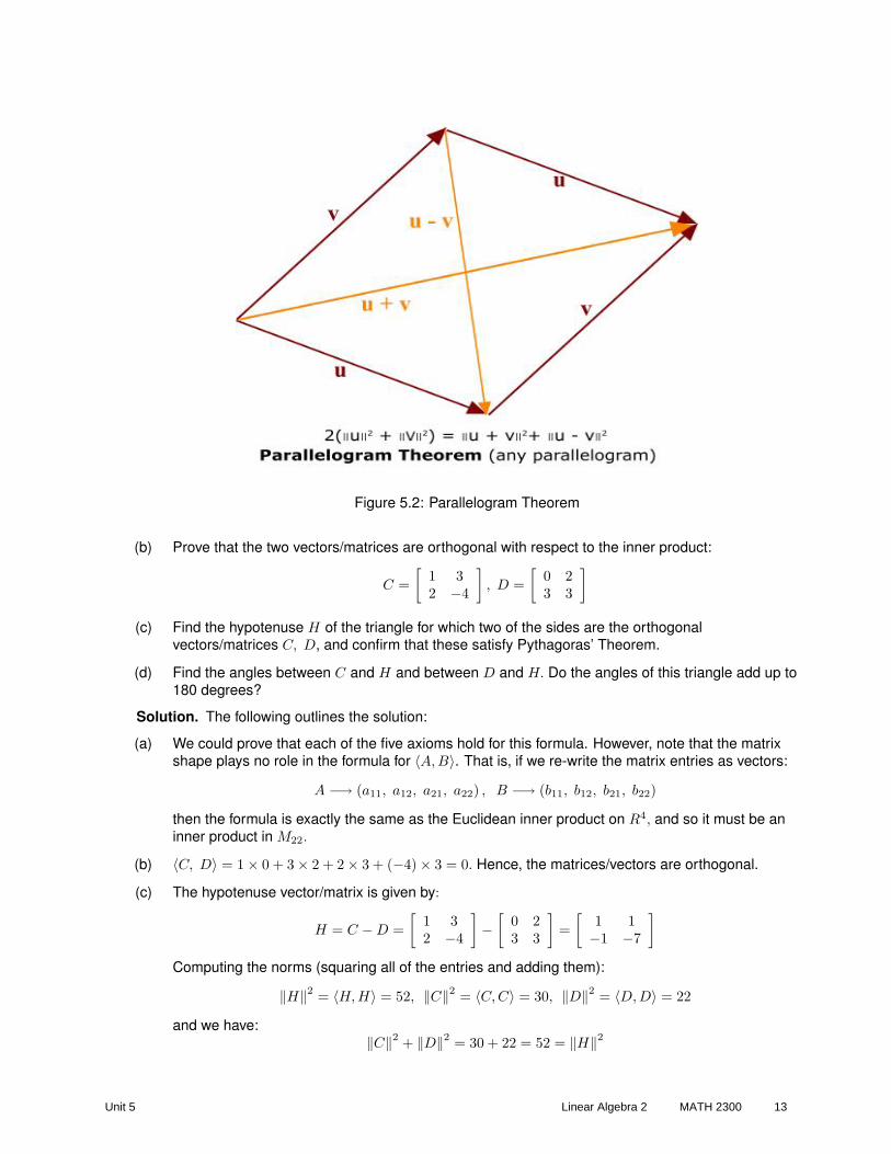
Figure 5.2: Parallelogram Theorem

(b) Prove that the two vectors/matrices are orthogonal with respect to the inner product:

C =[

1 32 −4

], D =

[0 23 3

]

(c) Find the hypotenuse H of the triangle for which two of the sides are the orthogonalvectors/matrices C, D, and confirm that these satisfy Pythagoras’ Theorem.

(d) Find the angles between C and H and between D and H. Do the angles of this triangle add up to180 degrees?


(a) We could prove that each of the five axioms hold for this formula. However, note that the matrixshape plays no role in the formula for 〈A,B〉. That is, if we re-write the matrix entries as vectors:

A −→ (a11, a12, a21, a22) , B −→ (b11, b12, b21, b22)

then the formula is exactly the same as the Euclidean inner product on R4, and so it must be aninner product in M22.

(b) 〈C, D〉 = 1× 0 + 3× 2 + 2× 3 + (−4)× 3 = 0. Hence, the matrices/vectors are orthogonal.

(c) The hypotenuse vector/matrix is given by:

H = C −D =[

1 32 −4

]−

[0 23 3

]=

[1 1−1 −7

]

Computing the norms (squaring all of the entries and adding them):

‖H‖2 = 〈H,H〉 = 52, ‖C‖2 = 〈C, C〉 = 30, ‖D‖2 = 〈D,D〉 = 22

and we have:‖C‖2 + ‖D‖2 = 30 + 22 = 52 = ‖H‖2


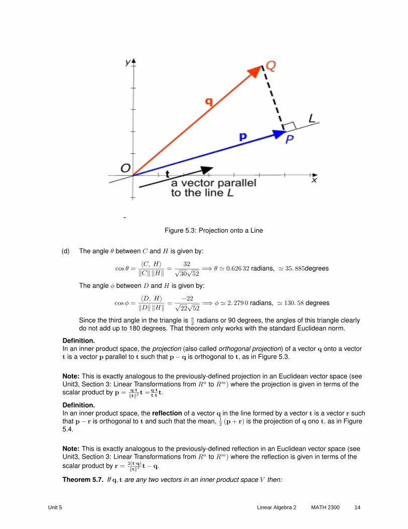
Figure 5.3: Projection onto a Line

(d) The angle θ between C and H is given by:

cos θ =〈C, H〉‖C‖ ‖H‖ =

32√30√

52=⇒ θ ' 0.626 32 radians, ' 35. 885degrees

The angle φ between D and H is given by:

cos φ =〈D, H〉‖D‖ ‖H‖ =

−22√22√

52=⇒ φ ' 2. 279 0 radians, ' 130. 58 degrees

Since the third angle in the triangle is π2 radians or 90 degrees, the angles of this triangle clearly

do not add up to 180 degrees. That theorem only works with the standard Euclidean norm.

Definition.In an inner product space, the projection (also called orthogonal projection) of a vector q onto a vectort is a vector p parallel to t such that p− q is orthogonal to t, as in Figure 5.3.

Note: This is exactly analogous to the previously-defined projection in an Euclidean vector space (seeUnit3, Section 3: Linear Transformations from Rn to Rm) where the projection is given in terms of thescalar product by p = q·t

‖t‖2 t =q·tt·t t.

Definition.In an inner product space, the reflection of a vector q in the line formed by a vector t is a vector r suchthat p− r is orthogonal to t and such that the mean, 1

2 (p + r) is the projection of q ono t, as in Figure5.4.

Note: This is exactly analogous to the previously-defined reflection in an Euclidean vector space (seeUnit3, Section 3: Linear Transformations from Rn to Rm) where the reflection is given in terms of thescalar product by r = 2(t·q)

‖t‖2 t− q.

Theorem 5.7. If q, t are any two vectors in an inner product space V then:


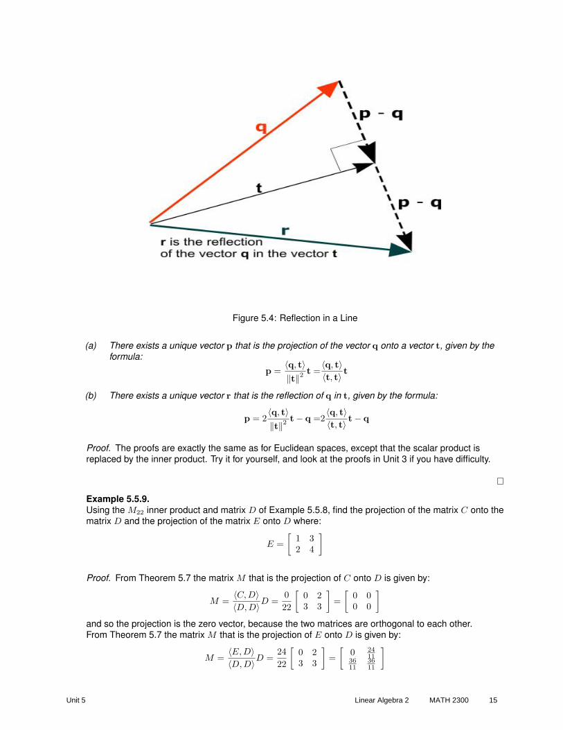
Figure 5.4: Reflection in a Line

(a) There exists a unique vector p that is the projection of the vector q onto a vector t, given by theformula:

p =〈q, t〉‖t‖2 t =

〈q, t〉〈t, t〉 t

(b) There exists a unique vector r that is the reflection of q in t, given by the formula:

p = 2〈q, t〉‖t‖2 t− q =2

〈q, t〉〈t, t〉 t− q

Proof. The proofs are exactly the same as for Euclidean spaces, except that the scalar product isreplaced by the inner product. Try it for yourself, and look at the proofs in Unit 3 if you have difficulty.

Example 5.5.9.Using the M22 inner product and matrix D of Example 5.5.8, find the projection of the matrix C onto thematrix D and the projection of the matrix E onto D where:

E =[

1 32 4

]

Proof. From Theorem 5.7 the matrix M that is the projection of C onto D is given by:

M =〈C,D〉〈D, D〉D =

022

[0 23 3

]=

[0 00 0

]

and so the projection is the zero vector, because the two matrices are orthogonal to each other.From Theorem 5.7 the matrix M that is the projection of E onto D is given by:

M =〈E, D〉〈D, D〉D =

2422

[0 23 3

]=

[0 24

113611

3611

]


Example 5.5.10.Requires calculus. In P4 find the reflection of the polynomial f (x) = x in the polynomialg (x) = 1 + x + x2 + x3, using the inner product

∫ 1

−1f (x) g (x) dx.

Solution. The reflection polynomial h (x) is given by the formula:

h (x) = 2〈f, g〉〈g, g〉g (x)− f (x)

= 2

∫ 1

−1f (x) g (x) dx

∫ 1

−1f (x) g (x) dx

g (x)− g (x)

Section 5.5 exercise setCheck your understanding by answering the following questions.

1. In R2 prove that 〈u,v〉 is an inner product (show it satisfies the five axioms):

〈u,v〉 = 2u1v1 + 3u2v2

for any two vectors u = (u1, u2) and v = (v1, v2).

2. In R2 let any two vectors be given by u = (u1, u2) and v = (v1, v2) . Show that each of thefollowing is not an inner product in R2. Recall that you need only produce one example where theresult fails in order to disprove something.

(a) 〈u,v〉 = −2u1v1 + 3u2v2

(b) 〈u,v〉 = u1v1 + u2

(c) 〈u,v〉 = u1v1 + u2v2 + 1

(d) 〈u,v〉 = |u1v1 + u2v2| (absolute value)

(e) 〈u,v〉 = u1v1

+ u2v2

3. Using the inner product on R2 given by 〈u,v〉 = 2u1v1 + 3u2v2:

(a) Find the lengths of the vectors (1, 0) , (2, − 1) .

(b) Find the inner product of the two vectors above.

(c) Find the angle between the two vectors.

4. Define an inner product on R3 by:

〈(u1, u2, u3) , (v1, v2, v3)〉 = 2u1v1 + 3u2v2 + u3v3

(a) Find the length of the vector (3, 2, 1) .

(b) Find the inner product of the vector (3, 2, 1) with the vector (0, 1, − 2) .

(c) Find all vectors perpendicular to the vector (3, 2, 1) .

(d) Find the distance from (3, 2, 1) to (0, 1, − 2) .

5. Define an function on P3 for any two polynomials p (x) = a0 + a1x + a2x2, q (x) = b0 + b1x + b2x

2

by:〈p, q〉 = a0b0 + a1b1 + a2b2

(a) Prove that it is an inner product.

(b) Find the length of the vector p (x) = 2− 3x + 4x2.


(c) Find all vectors perpendicular to the vector p (x) = 1.

(d) Find all vectors perpendicular to the vector p (x) = 1 + 2x− x2.

6. Note: Requires calculus. Repeat the previous problem, parts (a), (b), (c), but with the innerproduct defined for any two polynomials in p, q ∈ P3 by:

〈p, q〉 =∫ 1

−1

p (x) q (x) dx

7. Using the matrix-based inner product for R2 defined by 〈u, v〉 = uT AT Av (see Examples 5.5.4and 5.5.5), where:

A =[

2 30 1

]

(a) Find the length of the vector (1, 1) .

(b) Find the inner product of the vector (1, 1) with the vector (0, 1) .

(c) Find the distance from (1, 1) to (0, 1) .

(d) Find the angle between the vectors (1, 1) and (0, 1) .

8. In R2 define a function 〈u, v〉 = uT AT Av where:

A =

1 00 11 1

Is it an inner product for R2? Justify your answer.

9. In R2 with inner product 〈u,v〉 = 2u1v1 + 3u2v2, find the equation satisfied by all vectors with‖u‖ = 1.

10. Find a formula for the inner product in P3 given in Theorem 5.1, when the basis of P3 is{1, x, 1 + x2

}.

11. In M22, for any two matrices A = [aij ] , B = [bij ] define:

〈A, B〉 = a11b11 + 2a12b12 + 3a21b21 + 4a22b22

That is, multipy elements in corresponding positions in each matrix and form a weighted sum.

(a) Show this is an inner product.

(b) Compute the norm of the matrix/vector given in question 7.

(c) Compute the inner product of the two matrices/vectors:

C =[

1 00 1

], D =

[0 31 0

]

(d) Compute the distance between the two matrices/vectors above.

(e) Compute the angle between the two matrices/vectors above.

12. Use the Cauchy-Schwarz inequality to prove:

(a) For any two vectors u,v ∈ R2

|u1v1 + u2v2| ≤(u2

1 + u22

) 12

(v21 + v2

2

) 12


(b) For any two vectors u,v ∈ Rn

|u1v1 + u2v2 + · · · + unvn| ≤(u2

1 + u22 + · · · + u2

n

) 12

(v21 + v2

2 + · · · + v2n

) 12

(c) Requires calculus. For any two functions f, g continuous on [0, 1]:

[∫ 1

0

f (x) g (x) dx

]2

≤[∫ 1

0

f (x) dx

] [∫ 1

0

g (x) dx

]

(d) Requires calculus. For any two functions f, g continuous on [0, 1]:

[∫ 1

0

[f (x) + g (x)]2 dx

] 12

≤[∫ 1

0

[f (x)]2 dx

] 12

+[∫ 1

0

[g (x)]2 dx

] 12

13. Let V be any inner product space. Prove that the inner product function can be expressed interms of norms of the vectors by:

〈u, v〉 =14‖u + v‖2 − 1

4‖u− v‖2

14. Show that Pythagoras’ Theorem can be written in the following form and prove this result. For allnon-zero vectors p, q, r satisfying (p− r) · (r− q) = 0, it is true that:

‖p− r‖2 + ‖r− q‖2 = ‖p− q‖2

15. In any inner product space prove that if ‖v‖ = 0 then v = 0 (the zero vector).

16. If V is an inner product space then prove:

(a) If u ∈ V , is a fixed vector then prove that the set S = {v ∈ V | 〈u,v〉 = 0} , of all vectorsperpendicular to u, is a subspace of V.

(b) If w is perpendicular to each of the vectors in T = {v1,v2, · · · vk} then w is perpendicularto every vector in the linear span of T (that is, all linear combinations of the vectors vj).

(c) The set S of all vectors w ∈ V perpendicular to T is a subspace of V . Note: Sometime S isdesignated by the symbol T⊥.

(d) If the set T in part (b) is a basis of V then w must be the zero vector (that is, only the zerovector is perpendicular to every vector of a basis).

17. In an inner product space V prove that any three vectors satisfy:

‖v1 + v2 + v3‖ ≤ ‖v1‖+ ‖v2‖+ ‖v3‖

Solutions

1. 〈u,v〉 = 2u1v1 + 3u2v2 is clearly a real number so Axiom 1 is satisfied, and clearly〈u,v〉 = 〈v,u〉 = 2u1v1 + 3u2v2 so Axiom 2 is satisfied.Axiom 3 follows from the linearity of real number multiplication/addition:

〈u + w,v〉 = 2 (u1 + w1) v1 + 3 (u2 + w2) v2

= 2u1v1 + 3u2v2 + 2w1v1 + 3w2v2

= 〈u,v〉+ 〈w,v〉


Axiom 4 follows in a similar way:

〈ku,v〉 = 2ku1 + k3u2

= k (2u1 + 3u2)= k 〈u,v〉

Axiom 5 follows easily:〈u,u〉 = 2u2

1 + 3u22 ≥ 0

and clearly 〈u,u〉 = 0 only if u1 = u2 = 0.

2. Note: In each case one Axiom is shown to fail, but it is noted that other Axioms fail as well. Tryyourself to find examples of failure for these other Axioms.

(a) 〈u,v〉 = −2u1v1 + 3u2v2 satisfies the first four axioms but Axiom 5 fails if, for example,u = (1, 0) when 〈u,u〉 = −2 is negative.

(b) 〈u,v〉 = u1v1 + u2 satisfies Axioms 1, but none of the other axioms. For example, Axiom 2fails when u = (1, 1) , v = (1, 0) because 〈u,v〉 = 2 6= 〈v,u〉 = 1.

(c) 〈u,v〉 = u1v1 + u2v2 + 1 satisfies Axioms 1, 2, 5 but not Axioms 3 and 4. For example, todisprove Axiom 3, if u = (1, 0) , v = (1, 1) , w = (1, 0) then:

〈u + w, v〉 = 3, 〈u, v〉+ 〈w, v〉 = 2 + 2 = 4

so 〈u + w, v〉 6= 〈u, v〉+ 〈w, v〉.(d) 〈u,v〉 = |u1v1 + u2v2| satisfies Axioms 1, 2, 5 but not Axioms 3 and 4. For example, to

disprove Axiom 4, if u = (1, 0) , v = (1, 0) , k = −2 then:

〈u, v〉 = 1, 〈ku, v〉 = 2, k 〈u, v〉 = −2

so 〈ku, v〉 6= k 〈u, v〉.(e) 〈u,v〉 = u1

v1+ u2

v2does not satisfy any of the axioms. For example, Axiom 1 does not hold if

u = (1, 0) because 〈u,v〉 is not defined (cannot divide by zero).

3. If u = (1, 0) ,v = (2, − 1) , 〈u,v〉 = 2u1v1 + 3u2v2, then:

(a) ‖u‖ =√〈u,u〉 =

√2u2

1 + 3u22 =

√2. Similarly ‖v‖ =

√11.

(b) 〈u, v〉 = 2u1v1 + 3u2v2 = 4

(c) The angle θ between 0 and π is given by cos θ = 〈u,v〉‖u‖‖v‖ = 4√

22, and it is approximately (using

a calculator): θ = arccos(

4√22

)' 0.549 47 radians (or 31. 482 degrees). Note: This is not the

usual angle between these two vectors given by the Euclidean norm, which is about 0.463 65radians or 26. 565 degrees -check this for yourself.

4. If 〈(u1, u2, u3) , (v1, v2, v3)〉 = 2u1v1 + 3u2v2 + u3v3 and u = (3, 2, 1) ,v = (0, 1, − 2) then:

(a) ‖u‖ =√〈u,u〉 =

√2u2

1 + 3u22 + u2

3 =√

31

(b) 〈u,v〉 = 2u1v1 + 3u2v2 + u3v3 = 4

(c) The vector w = (w1, w2, w3) is perpendicular to u if:

2u1w1 + 3u2w2 + u3w3 = 0 =⇒6w1 + 6w2 + w3 = 0

This is the equation of a plane through the origin. That is, all vectors from the origin to apoint on this plane are perpendicular to u.


(d) ‖u− v‖ =√〈u− v,u− v〉 =

√(3, 1, 3) , (3, 1, 3) =

√30

5. If f (x) = a0 + a1x + a2x2, g (x) = b0 + b1x + b2x

2 and 〈f, g〉 = a0b0 + a1b1 + a2b2 then:

(a) Axioms 1 and 2 clearly hold since a0b0 + a1b1 + a2b2 is a real number, and the real numbermultiplications are all commutative. Axiom 3 holds because if h (x) = c0 + c1x + c2x

2 then:

〈f + h, g〉 = (a0 + c0) b0 + (a1 + c1) b1 + (a2 + c2) b2

= (a0b0 + a1b1 + a2b2) + (c0b0 + c1b1 + c2b2)= 〈f, g〉+ 〈h, g〉

Axiom 4 holds because:〈f, f〉 = a2

0 + a21 + a2

2 ≥ 0

and 〈f, f〉 = 0 only if a0 = a1 = a2 = 0 (that is, when f (x) is the zero function).(b) ‖p (x)‖ =

√〈p, p〉 =

√p20 + p2

1 + p22 =

√29

(c) q (x) = q0 + q1x + q2x2 is perpendicular to p (x) = p0 + p1x + p2x

2 = 1 if:

q0p0 + q1p1 + q2p2 = 0 =⇒q0 = 0 (since p0 = 1, p1 = p2 = 0)

Hence, the vectors/polynomials perpendicular to p (x) = 1 are all polynomials of the formq (x) = q1x + q2x

2 for any real values q1, q2.

(d) Similar to the previous part q (x) must satisfy:

q0p0 + q1p1 + q2p2 = 0

where p0 = 1, p1 = 2, p2 = −1. That is:

q0 + 2q1 − q2 = 0

That is, replacing q2 by (q0 + 2q1) , all vectors/polynomials perpendicular top (x) = 1 + 2x− x2 are q (x) = q0 + q1x + (q0 + 2q1)x2, for any real values q0, q1.

6. If f (x) = a0 + a1x + a2x2, g (x) = b0 + b1x + b2x

2 and 〈f, g〉 =∫ 1

−1p (x) q (x) dx then:

(a) Axiom 1 holds because the integral always exists (when the functions are continuous) and isa real number.Axiom 2 holds because 〈f, g〉 = 〈g, f〉 =

∫ 1

−1f (x) g (x) dx.

Axiom 3 holds because if h (x) = c0 + c1x + c2x2 then:

〈f + h, g〉 =∫ 1

−1

(f (x) + h (x)) g (x) dx

=∫ 1

−1

f (x) g (x) + h (x) g (x) dx

=∫ 1

−1

f (x) g (x) dx +∫ 1

−1

h (x) g (x) dx

= 〈f, g〉+ 〈h, g〉Axiom 4 holds because if k ∈ R:

〈kf, g〉 =∫ 1

−1

kf (x) g (x) dx

= k

∫ 1

−1

f (x) g (x) dx

= k 〈f, g〉


Axiom 5 holds because:

〈f, f〉 =∫ 1

−1

[f (x)]2 dx ≥ 0

since the integral of a non-negative function over any interval is a non-negative value. Atheorem of calculus shows that the only way this integral can be equal to zero when f iscontinous on the interval [−1, 1] is when f (x) is equal to zero for every x in the interval.Note: This proof also works for the vector space of functions for which the integrals exist,such as the vector space of all functions continuous on [−1, 1]. The proof also works ifdifferent limits of integration are used to define the inner product formula.

(b) ‖p (x)‖ =√〈p, p〉 =

√∫ 1

−1[p (x)]2 dx and this is given by:

√∫ 1

−1

[p (x)]2 dx =

√∫ 1

−1

(2− 3x + 4x2)2 dx

=

√∫ 1

−1

(16x4 − 24x3 + 25x2 − 12x + 4) dx

=

√165

x5 − 6x4 +253

x3 − 6x2 + 4x

∣∣∣∣1

−1

=

√46615

(c) q (x) = q0 + q1x + q2x2 is perpendicular to p (x) = p0 + p1x + p2x

2 = 1 if:

0 = 〈p, q〉 =∫ 1

−1

p (x) q (x) dx

0 =∫ 1

−1

(q0 + q1x + q2x

2)

dx

0 = q0x + q1x2

2+ q2

x3

3

∣∣∣∣1

−1

0 = 2q0 +23q2

0 = q0 +q2

3

Hence, substituting q0 = − q23 , the polynomials perpendicular to p (x) = 1 are

q (x) = − q23 + q1x + q2x

2.

7. Let u = (1, 1) , v = (0, 1) . First compute:

AT A =[

2 03 1

] [2 30 1

]=

[4 66 10

]

(a) ‖u‖ =√〈u,u〉 =

√uT AT Au and this is given by:

uT AT Au =[

1 1] [

4 66 10

] [11

]= 26

Hence, ‖u‖ =√

26. Similarly, ‖v‖ =√

10.


(b) This is given by:

〈u,v〉 = uT AT Av =[

1 1] [

4 66 10

] [01

]= 16

(c) ‖u− v‖ =√〈u− v,u− v〉 and 〈u− v,u− v〉 is given by:

〈u− v,u− v〉 = (u− v)TAT A (u− v)

=[

1 0] [

4 66 10

] [10

]

= 4

Hence, the distance from (1, 1) to (0, 1) is√

4 = 2.

(d) The angle θ between u and v is given by:

cos θ =〈u,v〉‖u‖ ‖v‖ =

16√26√

10=

8√65

The approximate angle (using a calculator) is θ = arccos 8√65' 0.124 35 radians or about 7.

124 7 degrees. Note: This has no relationship to the angle calculated using the Euclideaninner product, which is π

4 or 45 degrees.

8. The function 〈u, v〉 = uT AT Av is defined for all vectors u, v ∈ R2 and is a real number (sincethe sizes of the four parts of the product are compatible: 1× 2, 2× 3, 3× 2, 2× 1, and the resulthas size 1× 1). Hence, Axiom 1 is satisfied.Axiom 2 is satisfied because 〈v, u〉 = vT AT Au =

(vT AT Au

)T (since the transpose of a numberis the same number). Hence:

〈v, u〉 =(vT AT Au

)T= uT AT A v = 〈u,v〉

Axiom 3 is satisfied since:

〈u + w, v〉 = (u + w)TAT A v

= uT AT Av + wT AT A v

= 〈u, v〉+ 〈w, v〉Axiom 4 is satisfed since for k ∈ R:

〈ku,v〉 = (ku)TAT Av

= k(uT AT Av

)

= k 〈u,v〉Axiom 5 is satisfied since:

〈v,v〉 = vT AT Av

= (Av)T

= ‖Av‖2 (standard Euclidean norm)

and so 〈v,v〉 = ‖Av‖2 ≥ 0. Furthermore, Av = 0 only if:

1 00 11 1

[v1

v2

]=

000

=⇒

v1

v2

v1 + v2

=

000

which shows v = 0.Hence, all five axioms are satisfied and so the function is an inner product.


9. ‖u‖ = 1 if, and only if, ‖u‖2 = 1, which is 2u21 + 3u2

2 = 1. In the standard Euclidean axis system,this is an ellipse.

10. Any vector/polynomial p (x) = p0 + p1x + p2x2 can be expressed in terms of the basis by:

p (x) = (p0 − p2)× 1 + p1 × x + p2 ×(1 + x2

)

Hence, by Theorem 5.1 the inner product defined as a dot product by this basis is:

〈p, q〉 = (p0 − p2, p1, p2) · (q0 − q2, q1, q2)= (p0 − p2) (q0 − q2) + p1q1 + p2q2

〈p, q〉 = p0q0 − p0q2 + p1q1 − p2q0 + 2p2q2

Hence, the inner product is:

〈p, q〉 = p0q0 − p0q2 + p1q1 − p2q0 + 2p2q2

11.

(a) We could prove that each of the five axioms hold for this formula. However, we can avoid thisby using the method of Example 5.5.8. Note that the matrix shape plays no role in theformula for 〈A,B〉. The formula is exactly the same as a weighted (weights 1, 2, 3, and 4)Euclidean inner product on R4 where the matrix entries are re-written as vectors:

A −→ (a11, a12, a21, a22) , B −→ (b11, b12, b21, b22)

Since a weighted Euclidean inner product is always an inner product, then the matrix formula〈A,B〉 is also an inner product.

(b)∥∥∥∥[

2 30 1

]∥∥∥∥ = 1× 22 + 2× 32 + 3× 0 + 4× 12 = 26

(c) 〈C, D〉 = 1× 0 + 2× 0× 3 + 3× 0× 1 + 4× 1× 0 = 0

(d) 〈C −D, C −D〉 =⟨[

1 −3−1 1

],

[1 −3−1 1

]⟩= 1 + 2 (−3)2 + 3 (−1)2 + 4 = 26. Hence:

‖C −D‖ =√〈C −D, C −D〉 =

√26

(e) If θ is the angle between C and D then:

cos θ =〈C, D〉‖C‖ ‖D‖ = 0 since 〈C,D〉 = 0

Hence, θ = π2 (90 degrees). The matrices are perpendicular to each other.

12. The Cauchy-Schwarz result (Theorem 5.3) is: |〈u,v〉| ≤ ‖u‖ ‖v‖.(a) If u = (u1, u2) , v = (v1, v2) with the inner product is the standard scalar or dot product so

that 〈u,v〉 = u1v1 + u2v2 and ‖u‖ =√

u21 + u2

2, ‖v‖ =√

v21 + v2

2 . Applying these in theCauchy-Schwarz formula gives the required result:

|u1v1 + u2v2| ≤√

u21 + u2

2

√v21 + v2

2

(b) The proof is very similar to part (a). Try this for yourself.


(c) The function 〈f, g〉 =∫ 1

0f (x) g (x) dx is an inner product for the vector space of functions

continuous on [0, 1] (see the proof of question 6(a). With this inner product:

‖f‖ =√∫ 1

0[f (x)]2 dx, ‖g‖ =

√∫ 1

0[g (x)]2 dx, and the Cauchy-Schwarz result,

|〈f, g〉| ≤ ‖f‖ ‖g‖, becomes:∣∣∣∣∫ 1

0

f (x) g (x) dx

∣∣∣∣ ≤(∫ 1

0

[f (x)]2 dx

) 12

(∫ 1

0

[g (x)]2 dx

) 12

Both sides are positive, so squaring both sides gives the required result:[∫ 1

0

f (x) g (x) dx

]2

≤[∫ 1

0

[f (x)]2 dx

] [∫ 1

0

[g (x)]2 dx

]

(d) This result is simply the triangle inequality (see Theorem 5.4, part (c)):

‖f + g‖ ≤ ‖f‖+ ‖g‖13. By the definition of norm in terms of the inner product and the axioms of the inner product:

14‖u + v‖2 − 1

4‖u− v‖2 =

14〈u + v,u + v 〉 − 1

4〈u− v, u− v〉

=14

[〈u,u 〉+ 2 〈u,v〉+ 〈v,v 〉]− 14

[〈u,u 〉 − 2 〈u,v〉+ 〈v,v 〉]= 〈u,v〉

14. One version of Pythagoras’ Theorem (Theorem 5.5) states that ‖u‖2 + ‖v‖2 = ‖u + v‖2 when〈u,v〉 = 0. Replace u by p− r and v by r− q so that u + v is replaced by p− q and 〈u,v〉 = 0 isreplaced by 〈p− r, r− q〉 = 0, thus giving the required result:

‖p− r‖2 + ‖r− q‖2 = ‖p− q‖2

15. Proof of the ”if” part: If v = 0 then 〈v,v〉 = 0 by Axiom 5. Hence, ‖v‖ =√〈v,v〉 = 0.

Proof of the ”only if” part: If ‖v‖ = 0 then ‖v‖2 = 〈v,v〉 = 0. Axiom 5 states that 〈v,v〉 = 0 onlywhen v = 0 and so the result follows.

16.

(a) The set S of vectors in V perpendicular to a particular vector v is a subset of a vector spaceV. To prove S is a vector space it is only necessary to prove it is closed under addition andscalar multiplication (see Theorem 2.3 of Unit 2, Section 3: Subspaces of a Vector Space).Suppose k ∈ R and v, w are any two vectors in S, so 〈v,u〉 = 〈w,u〉 = 0. Using the axiomsof the inner product:

〈v + w,u〉 = 〈v,u〉+ 〈w,u〉 = 0 + 0 = 0〈kv,u〉 = k 〈v,u〉 = k × 0 = 0

Hence, S is closed under addition and scalar multiplication and so it is a vector space (asubspace of V ). Note: S must also be an inner product space since the inner product of V isalso an inner product for S.

(b) If w satisfies 〈v1, w〉 = 0, 〈v2, w〉 = 0, · · · , 〈vk, w〉 = 0 and then by the axioms of innerproducts, for any scalars r1, r2, · · · , rk :

〈r1v1 + r2v2 + · · · + rkvk, w〉 = 〈r1v1, w〉+ 〈r2v2, w〉+ · · · + 〈rkvk, w〉= r1 〈v1, w〉+ r2 〈v2, w〉+ · · · + rk 〈vk, w〉= 0

Hence, w is perpendicular to the linear span of T.


(c) As in part (a), it is only necessary to prove that S is closed under addition and scalarmultiplication. The proof is very similar to the proof of part (a) and is not given here.

(d) The vector w is perpendicular to all of the basis vectors, and w is also a linear combinationof the basis vectors. However w is orthogonal to all linear combinations of the basis vectors,by part (b), and so w is perpendicular to itself:

0 = 〈w, w〉By Axiom 5 for linear products, it follows that w = 0.

17. The triangle inequality for any two vectors u, v ∈ V, states that ‖u + v‖ ≤ ‖u‖+ ‖v‖ . Writingu = v1 + v2 and v = v3 changes this to:

‖(v1 + v2) + v3‖ ≤ ‖v1 + v2‖+ ‖v3‖Applying the triangle inequality a second time to v1,v2 shows that ‖v1 + v2‖ ≤ ‖v1‖+ ‖v2‖ andso the above inequality becomes the required result:

‖v1 + v2 + v3‖ ≤ ‖v1‖+ ‖v2‖+ ‖v3‖

5.6 Orthogonal bases, the Gram-Schmidt process and QR− fac-torization

We have previously seen that a basis of a vector space can be used to develop most processes andproperties of interest. Usually it does not matter which particular basis is used, but sometimes a specialbasis is easier to use than other bases. In particular, if the vector space is an Inner Product Space thenit is often very advantageous to work with an orthogonal basis (each basis vector is perpendicular toevery other basis vector). Orthogonal bases are required in some applications, such as the method fordiagonalizing a matrix using eigenvalues and eigenvectors (see Unit 4 Eigenvalues, Eigenvectors, andDiagonalization of Matrices, Diagonalizing a Matrix).

In this section an algorithm , the Gram-Schmidt Process, is described for converting anynon-orthogonal basis of an Inner Product Space into an orthogonal basis. If the vectors of the originalbasis are the columns of a matrix A then the Gram-Schmidt process is shown to be equivalent tofinding a QR− factorization, A = QR, where Q is an orthogonal matrix, and R is upper triangular. TheQR− factorization is used in the QR− algorithm, one of the most successful numerical methods forfinding the eigenvalues a matrix (see Unit 4 Eigenvalues, Eigenvectors and Diagonalization of Matrices,Methods for finding Eigenvalues and Eigenvectors).

5.6.1 The Gram-Schmidt processDefinition.A set of vectors {v1, v2, v3, · · · , vn} of an Inner Product space is said to be orthogonal if the vectorsare mutually orthogonal, meaning:

〈vi, vj〉 = 0 for i 6= j = 1, 2, 3, · · · , n

The set {v1, v2, v3, · · · , vn} is said to be orthonormal if it is orthogonal and all vectors are unitvectors. That is, for i, j = 1, 2, 3, · · · , n:

〈vi, vi〉 = 1 and 〈vi, vj〉 = 0 if i 6= j

Note: A vector v is a unit vector if its length is 1, meaning ‖v‖ = 1. Since ‖v‖2 = 〈v, v〉 , and so‖v‖ =

√〈v, v〉, it follows that v is also a unit vector if 〈v, v〉 = 1.

Note: An orthogonal set of vectors can always be converted to an orthonormal set by simply convertingeach vector to a unit vector by dividing it by its length (change each vector v to the vector

1‖v‖v = 1√

〈v, v〉v).


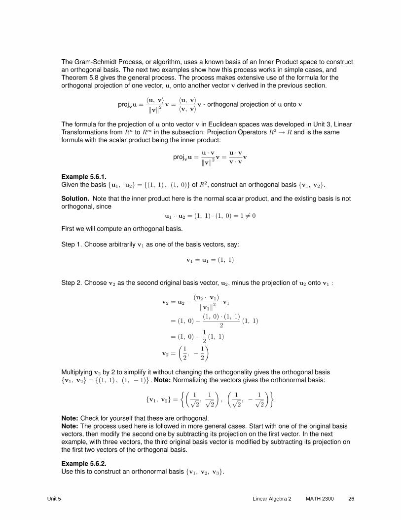
The Gram-Schmidt Process, or algorithm, uses a known basis of an Inner Product space to constructan orthogonal basis. The next two examples show how this process works in simple cases, andTheorem 5.8 gives the general process. The process makes extensive use of the formula for theorthogonal projection of one vector, u, onto another vector v derived in the previous section.

projvu =〈u, v〉‖v‖2 v =

〈u, v〉〈v, v〉v - orthogonal projection of u onto v

The formula for the projection of u onto vector v in Euclidean spaces was developed in Unit 3, LinearTransformations from Rn to Rm in the subsection: Projection Operators R2 → R and is the sameformula with the scalar product being the inner product:

projvu =u · v‖v‖2 v =

u · vv · vv

Example 5.6.1.Given the basis {u1, u2} = {(1, 1) , (1, 0)} of R2, construct an orthogonal basis {v1, v2}.

Solution. Note that the inner product here is the normal scalar product, and the existing basis is notorthogonal, since

u1 · u2 = (1, 1) · (1, 0) = 1 6= 0

First we will compute an orthogonal basis.

Step 1. Choose arbitrarily v1 as one of the basis vectors, say:

v1 = u1 = (1, 1)

Step 2. Choose v2 as the second original basis vector, u2, minus the projection of u2 onto v1 :

v2 = u2 − (u2 · v1)‖v1‖2

v1

= (1, 0)− (1, 0) · (1, 1)2

(1, 1)

= (1, 0)− 12

(1, 1)

v2 =(

12, − 1

2

)

Multiplying v2 by 2 to simplify it without changing the orthogonality gives the orthogonal basis{v1, v2} = {(1, 1) , (1, − 1)} . Note: Normalizing the vectors gives the orthonormal basis:

{v1, v2} ={(

1√2,

1√2

),

(1√2, − 1√

2

)}

Note: Check for yourself that these are orthogonal.Note: The process used here is followed in more general cases. Start with one of the original basisvectors, then modify the second one by subtracting its projection on the first vector. In the nextexample, with three vectors, the third original basis vector is modified by subtracting its projection onthe first two vectors of the orthogonal basis.

Example 5.6.2.Use this to construct an orthonormal basis {v1, v2, v3}.


Solution. Note that the inner product here is the normal scalar product, and the existing basis isclearly not orthogonal. It is easiest to construct an orthogonal basis first, then normalize (make into unitvectors) the basis afterwards. Start as in the previous example:

Step 1. Choose arbitrarily v1 as one of the basis vectors, say:

v1 = u1 = (1, 1, 1)

Step 2. You might notice that u2 is already orthogonal to v1 and so we can choosev2 = u2 = (1, 0 − 1) . If you did not notice this then the solution process gives the same result asfollows. Choose v2 as the second original basis vector, u2, minus the projection of u2 onto v1 :

v2 = u2 − (u2 · v1)‖v1‖2

v1

= (1, 0, − 1)− (1, 0, − 1) · (1, 1, 1)(1, 1, 1) · (1, 1, 1)

(1, 1, 1)

= (1, 0 − 1)− 03

(1, 1, 1)

v2 = (1, 0 − 1)

Step 3. In order to find v3 apply the method of Step 2 to u3, but this time subtract off the projections ofu3 onto both v1 and v2.

v3 = u3 − (u3 · v1)‖v1‖2

v1 − (u3 · v2)‖v2‖2

v2

= (2, − 3, 4)− (2, − 3, 4) · (1, 1, 1)(1, 1, 1) · (1, 1, 1)

(1, 1, 1)− (2, − 3, 4) · (1, 0, − 1)(1, 0, − 1) · (1, 0, − 1)

(1, 0, − 1)

= (2, − 3, 4)− 33

(1, 1, 1)− −22

(1, 0, − 1)

v3 = (2, − 4, 2)

Hence, the orthogonal basis is {v1, v2, v3} = {(1, 1, 1) , (1, 0 − 1) , (2,−4, 2)} .Note: Check for yourself that this set is orthogonal. Notice that v3 = (1, − 2, 1) can be simplified, bydividing by 2, to give v3 = (1, − 2, 1), and the set is still orthogonal.Note: Normalizing the orthogonal basis gives an orthonormal basis:

{v1, v2, v3} ={(

1√3,

1√3,

1√3

),

(1√2, 0 − 1√

2

),

(1√6,− 2√

6,

1√6

)}

The general method for producing an orthogonal basis is given next in Theorem 5.8. It is a simpleextension of the process in Examples 5.6.1 and 5.6.2 above, except that a dot product like u2 · v1 isreplaced by the inner product 〈u2, v1〉 .Theorem 5.8. The Gram-Schmidt Process If {u1, u2, u3, · · · , um} is a set of linearly independentvectors spanning a subspace S of an inner-product space V then an orthogonal set of vectors,{v1, v2, v3, · · · , vm} , spanning the same subspace S is produced by the following process(algorithm):

Step 1. Set v1 = u1

Step 2. Set v2 = u2 − 〈u2, v1〉‖v1‖2

v1


Step 3. Set v3 = u3 − 〈u3, v1〉‖v1‖2

v1 − 〈u3, v2〉‖v2‖2

v2

Step 4. Set v4 = u4 − 〈u4, v1〉‖v1‖2

v1 − 〈u4, v2〉‖v2‖2

v2 − 〈u4, v3〉‖v3‖2

v3

and continuing this pattern until step m is reached:

Step m. Set vm = um − 〈um, v1〉‖v1‖2

v1 − 〈um, v2〉‖v2‖2

v2 − 〈um, v3〉‖v3‖2

v3− · · · · · · − 〈um, vm−1〉‖vm−1‖2

vm−1

Note: In the equations above we can replace ‖vj‖2 by 〈vj , vj〉 for each j = 1, 2, · · · ,m, and anorthonormal basis is obtained by changing each vj into the unit vector 1

‖vj‖vj = 1√〈vj , vj〉

vj .

Note: If {u1, u2, u3, · · · , um} is a basis of V then {v1, v2, v3, · · · , vm} will be an orthogonal basis ofV.

Proof. Consult your textbook or other source for a proof of this result. The proof is conceptually simplebut rather ”messy” and confusing.

The Gram-Schmidt Process can be written in a slightly different and, in some ways, simpler form inorder to directly produce an orthonormal basis, as in the next theorem.

Theorem 5.9. If {u1, u2, u3, · · · , um} is a set of linearly independent vectors spanning a subspace Sof an inner-product space V then an orthonormal set of vectors, {w1, w2, w3, · · · , wm} , spanningthe same subspace S is produced by the following process (algorithm):

Step 1. Set v1 = u1 and define w1 = 1‖v1‖v1. That is, normalize the vector v1 so it has length one by

dividing by ‖v1‖ =√〈v1, v1〉.

Step 2. Set v2 = u2 − 〈u2, w1〉w1 and define w2 = 1‖v2‖v2.

Step 3. Set v3 = u3 − 〈u3, w1〉w1 − 〈u3, w2〉w2 and define w3 = 1‖v3‖v3.

Step 4. Set v4 = u4 − 〈u4, w1〉w1 − 〈u4, w2〉w2 − 〈u4, w3〉w3 and define w4 = 1‖v4‖v4,

and continuing this pattern until step n is reached.

Step m. Set vm = um − 〈um, w1〉w1 − 〈um, w2〉w2 − 〈um, w3〉w3− · · · · · · − 〈uw, wm−1〉wm−1, anddefine wm = 1

‖vm‖vm.

Proof. In step 2 of Theorem 5.8 show that the formula there is the same as the one used here by


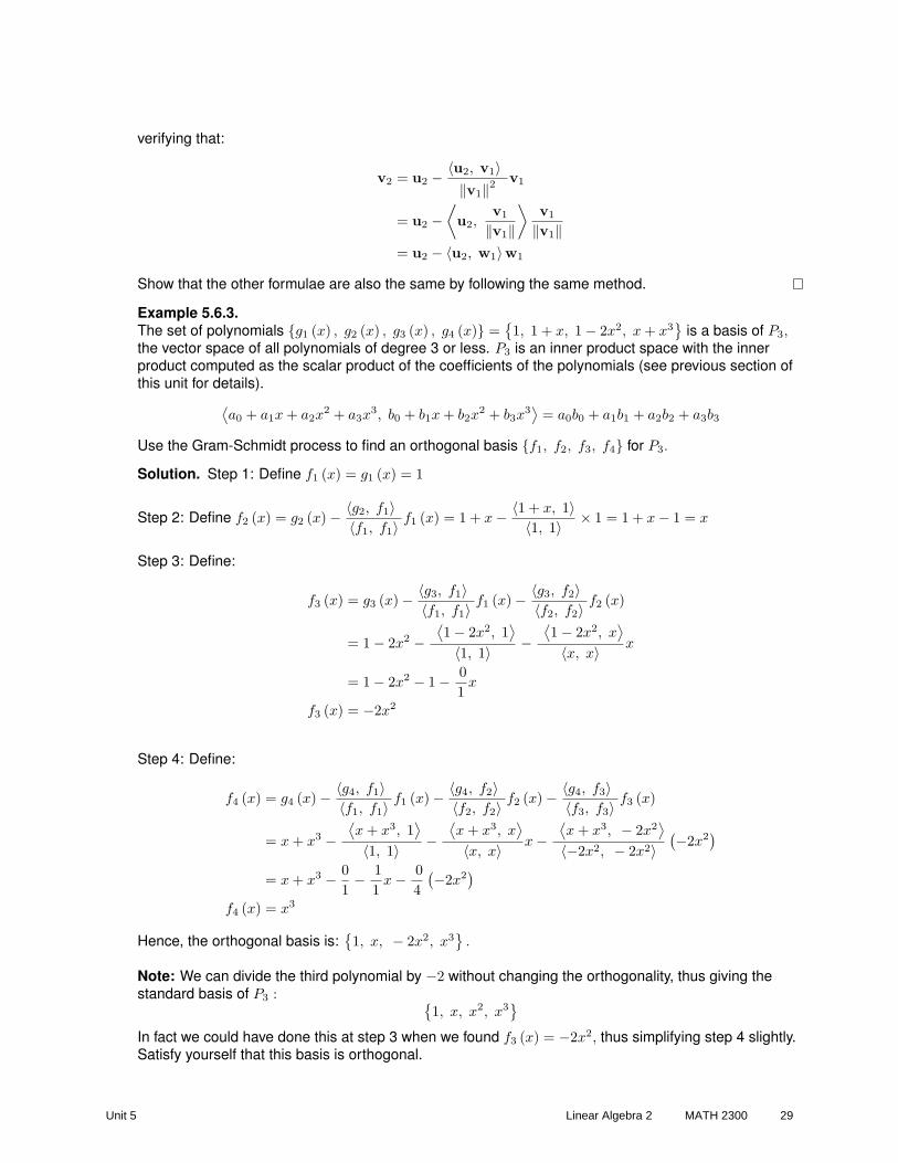
verifying that:

v2 = u2 − 〈u2, v1〉‖v1‖2

v1

= u2 −⟨u2,

v1

‖v1‖⟩

v1

‖v1‖= u2 − 〈u2, w1〉w1

Show that the other formulae are also the same by following the same method.

Example 5.6.3.The set of polynomials {g1 (x) , g2 (x) , g3 (x) , g4 (x)} =

{1, 1 + x, 1− 2x2, x + x3

}is a basis of P3,

the vector space of all polynomials of degree 3 or less. P3 is an inner product space with the innerproduct computed as the scalar product of the coefficients of the polynomials (see previous section ofthis unit for details).

⟨a0 + a1x + a2x

2 + a3x3, b0 + b1x + b2x

2 + b3x3⟩

= a0b0 + a1b1 + a2b2 + a3b3

Use the Gram-Schmidt process to find an orthogonal basis {f1, f2, f3, f4} for P3.

Solution. Step 1: Define f1 (x) = g1 (x) = 1

Step 2: Define f2 (x) = g2 (x)− 〈g2, f1〉〈f1, f1〉 f1 (x) = 1 + x− 〈1 + x, 1〉

〈1, 1〉 × 1 = 1 + x− 1 = x

Step 3: Define:

f3 (x) = g3 (x)− 〈g3, f1〉〈f1, f1〉 f1 (x)− 〈g3, f2〉

〈f2, f2〉 f2 (x)

= 1− 2x2 −⟨1− 2x2, 1

⟩

〈1, 1〉 −⟨1− 2x2, x

⟩

〈x, x〉 x

= 1− 2x2 − 1− 01

x

f3 (x) = −2x2

Step 4: Define:

f4 (x) = g4 (x)− 〈g4, f1〉〈f1, f1〉 f1 (x)− 〈g4, f2〉

〈f2, f2〉 f2 (x)− 〈g4, f3〉〈f3, f3〉 f3 (x)

= x + x3 −⟨x + x3, 1

⟩

〈1, 1〉 −⟨x + x3, x

⟩

〈x, x〉 x−⟨x + x3, − 2x2

⟩

〈−2x2, − 2x2〉(−2x2

)

= x + x3 − 01− 1

1x− 0

4(−2x2

)

f4 (x) = x3

Hence, the orthogonal basis is:{1, x, − 2x2, x3

}.

Note: We can divide the third polynomial by −2 without changing the orthogonality, thus giving thestandard basis of P3 : {

1, x, x2, x3}

In fact we could have done this at step 3 when we found f3 (x) = −2x2, thus simplifying step 4 slightly.Satisfy yourself that this basis is orthogonal.


Example 5.6.4.Requires calculus. The set of functions f (x) that are continuous on an interval [a, b] , written C [a, b]is a an infinite dimensional vector space and is an inner product space with the inner product definedas the integral of the product of the two functions between a and b :

〈f, g〉 =∫ b

a

f (x) g (x) dx

This is also an inner product for the subspaces of C [a, b] of polynomials Pn, n = 1, 2, 3, · · · . Givena = −1, b = 1 and the four functions: g1 (x) = 1, g2 (x) = x, g3 (x) = x2, g4 (x) = x3 then find fourorthogonal functions, f1, f2, f3, f4, that span the same subspace.

Solution. The following is the solution:

Step 1: Define f1 (x) = g1 (x) = 1

Step 2: Define:

f2 (x) = g2 (x)− 〈g2, f1〉〈f1, f1〉 f1 (x)

= x−∫ 1

−1x dx

∫ 1

−1dx

× 1

= x− 02

f2 (x) = x

Step 3: Define:

f3 (x) = g3 (x)− 〈g3, f1〉〈f1, f1〉 f1 (x)− 〈g3, f2〉

〈f2, f2〉 f2 (x)

= x2 −∫ 1

−1x2 dx

∫ 1

−1dx

× 1−∫ 1

−1x2 × x dx

∫ 1

−1x2 dx

x

= x2 −(

23

)

2− 0(

23

) x

f3 (x) = x2 − 13

Step 4: Define:

f4 (x) = g4 (x)− 〈g4, f1〉〈f1, f1〉 f1 (x)− 〈g4, f2〉

〈f2, f2〉 f2 (x)− 〈g4, f3〉〈f3, f3〉 f3 (x)

= x3 −∫ 1

−1x3 dx

∫ 1

−1dx

× 1−∫ 1

−1x3 × x dx

∫ 1

−1x2 dx

x−∫ 1

−1x3

(x2 − 1

3

)dx

∫ 1

−1

(x2 − 1

3

) (x2 − 1

3

)dx

(x2 − 1

3

)

= x3 − 02−

(25

)(

23

) x− 0(845

)(

x2 − 13

)

f4 (x) = x3 − 35

x


Note: The orthogonal polynomials f1 (x) = 1, f2 (x) = x, f3 (x) = x2 − 13 , f4 (x) = x2 − 3

5 x aremultiples of the first four Legendre Polynomials, which are:

p0 (x) = 1, p1 (x) = x, p2 (x) =12

(x2 − 1

), p3 (x) =

12

(5x3 − 3x

)

These multiples are chosen so that pk (1) = 1, so they are an orthogonal set but are not normalizedwith respect to the inner product and so do not form an orthonormal set. Legendre Polynomials areimportant in some Engineering applications and more details can be found on the web athttp://en.wikipedia.org/wiki/Legendre polynomials

5.6.2 Uses of orthogonal and orthonormal basesWhen vectors are expressed as linear combinations of orthogonal basis vectors, many operations aremuch easier to carry out, as is shown in the following theorems. If the basis is orthonormal, then itbecomes even easier, and vectors with respect to this orthonormal basis interact very like vectors inEuclidean spaces, Rn. The first theorem notes the fairly obvious fact that orthogonal sets of vectorsmust be linearly independent.

Theorem 5.10. If S = {v1, v2, v3, · · · , vn} is an orthogonal set of (non-zero) vectors in an innerproduct space then the vectors are linearly independent.Note: Hence, if S is produced by the Gram-Schmidt process applied to a basis of an inner productspace V , then S must also be a basis of V. Hence, every inner product space has an orthogonal basis.

Proof. If the vectors are linearly dependent then a non-zero linear combination of the vectors gives thezero vector:

k1v1 + k2v2 + k3v3 + · · · + knvn = 0

Take the inner product with v1, using the axioms:

〈(k1v1 + k2v2 + k3v3 + · · · + knvn) , v1〉 = 〈0, v1〉k1 〈v1, v1〉+ k2 〈v2, v1〉+ k3 〈v3, v1〉+ · · · + kn 〈vn, v1〉 = 0

k1 〈v1, v1〉 = 0

This shows that k1 = 0, since 〈v1, v1〉 = ‖v‖2 6= 0. Repeating the above process, taking inner productswith v2, v3, · · · , vn, shows that all of the coefficients are zero:

k1 = k2 = k3 = · · · = kn = 0

Hence, there is no linear combination of the vectors giving the zero vector except the trivial one with allcoefficients equal to zero, and so the vectors are linearly independent.

Theorem 5.11. If B = {b1, b2, b3, · · · , bn} is an orthonormal basis of an inner product space andvectors u,v have coordinates with respect to this basis:

(u)B = (u1, u2, u3, · · · , un) and (v)B = (v1, v2, v3, · · · , vn)

(that is: u = u1b1 + u2b2 + u3b3 + · · ·+ unbn and similarly for v), then:

(a) 〈u, v〉 = u1v1 + u2v2 + u3v3 + · · ·+ unvn

(b) ‖u‖ =√

u21 + u2

2 + u23 + · · ·+ u2

n

(c) d (u, v) =√

(u1 − v1)2 + (u2 − v2)

2 + (u3 − v3)2 + · · ·+ (un − vn)2


Note: These quantities do not depend on the values of the basis vectors, but only on the coordinatesrelative to the basis, and are exactly the same formulae as for Euclidean vectors in Rn with respect tothe standard basis of Rn.

Proof. The following is the proof:

(a) When n = 2: Using the linearity of the inner product:

〈u, v〉 = 〈u1b1 + u2b2 , v1b1 + v2b2〉= u1v1 〈b1, b1〉+ u1 v2 〈b1, b2〉+ u2v1 〈b2, b1〉+ u2v2 〈b2, b2〉

Using the orthonormality 〈b1, b1〉 = 〈b2, b2〉 = 1, and 〈b1, b2〉 = 〈b2, b1〉 = 0, this simplifies to:

〈u, v〉 = u1v1 + u2v2

Note: Try yourself the same proof for n = 3, and attempt to generalize your proof for all values of n.Note: Try yourself to prove (b) and (c) for the cases n = 2, 3 and for all n.

Theorem 5.12. If B = {v1, v2, v3, · · · , vn} is an orthogonal basis of an inner product space and avector u has coordinates (u)S = (u1, u2, u3, · · · , un) with respect to this basis then:

u1 =〈u, v1〉‖v1‖2

, u2 =〈u, v2〉‖v2‖2

, · · · , un =〈u, vn〉‖vn‖2

, so u =〈u, v1〉‖v1‖2

v1 +〈u, v2〉‖v2‖2

v2 + · · · +〈u, vn〉‖vn‖2

vn

If the basis is also orthonormal then:

u1 = 〈u, v1〉 , u2 = 〈u, v2〉 , · · · , un = 〈u, vn〉 so that u = 〈u, v1〉 v1+ 〈u, v2〉 v2+ · · · +〈u, vn〉 vn

Note: Recall that 〈u, v1〉‖v1‖2 v1 is the formula for the perpendicular projection of the vector u onto the

vector v1. Hence, the coordinates with respect to an orthogonal basis are given by the perpendicularprojections onto the basis vectors. Recall also that for any vector v, ‖v‖2 = 〈v, v〉 .

Proof. Proof for n = 2 : Suppose that u = u1v1 + u2v2 then taking the inner product with v1 and usingthe linearity axioms:

〈u, v1〉 = 〈u1v1 + u2v2, v1〉= u1 〈v1, v1〉+ u2 〈v2, v1〉

〈u, v1〉 = u1 〈v1, v1〉

Hence, solving for u1 :

u1 =〈u, v1〉〈v1, v1〉 =

〈u, v1〉‖v1‖2

Taking the inner product of u with v2 gives in the same way the formula for u2 :

u2 =〈u, v2〉〈v2, v2〉 =

〈u, v2〉‖v2‖2

Note: Try yourself the proof for n = 3, and think about the generalization to the proof for all n.


Generalizing the previous theorem to projections onto a subspace of an inner product space gives thefollowing result.

Theorem 5.13. Suppose that W is a r− dimensional subspace with orthogonal basisB = {v1, v2, · · · ,vr} of an inner product space V and u ∈ V, then:

(a) The perpendicular projection of u onto W is given by:

projW u =〈u, v1〉‖v1‖2

v1 +〈u, v2〉‖v2‖2

v2 + · · · +〈u, vr〉‖vr‖2

vr

or if {v1, v2, · · · ,vr} is orthonormal then:

projW u = 〈u, v1〉 v1 + 〈u, v2〉 v2 + · · · + 〈u, vr〉 vr

(b) The basis B can be extended to an orthogonal basis of V :

{v1, v2, · · · ,vr, vr+1, · · · ,vn}and the additional basis vectors vr+1, · · · ,vn are a basis of W⊥ (the subspace of all vectors inW that are perpendicular to every vector in W ).

(c) Every vector u ∈ V can be expressed in exactly one way:

u = u1 + u2 where u1 ∈ W and u2 ∈ W⊥

Note: Part (a) states that the projection of u onto W is simply the sum of the projections onto eachindividual vector of B (the orthogonal basis of W ).Note: The formula in part (a) for the projection of u onto the space S spanned by the orthogonal set{v1, v2, · · · ,vr} is exactly the same as the formula from Theorem 5.12. for expressing u as a linearcombination of the {v1, v2, · · · ,vr} . That is, the formula gives that linear combination if it exists (if uis in the span of S) and otherwise gives the projection of the vector u onto S.

Proof. The following is the proof:

(a) If w = projW u = k1v1 + k2v2 + · · · + krvr then use the fact that w − u is orthogonal to everyvector in W, first taking the inner product with v1:

0 = 〈w − u, v1〉0 = 〈k1v1 + k2v2 + · · · + krvr, v1〉 − 〈u, v1〉

Using the linearity of the inner product and orthonormality of B:

0 = k1 〈v1, v1〉 − 〈u, v1〉 =⇒

k1 =〈u, v1〉〈v1, v1〉 =

〈u, v1〉‖v1‖2

The formulae for other ki values can be established using the same method, computing0 =

⟨w − u, vj

⟩for j = 2, 3, · · · , r.

(b) (outline only) The basis B = {v1, v2, · · · ,vr} can be extended to a basis of V by first simplyadding any vector wr+1 not in W, then repeating this by adding another vector not in the span of{v1, v2, · · · ,vr, wr+1} and so on until a basis of V is created. Apply the Gram-Schmidt processto this basis, starting with v1, v2, · · · ,vr (i.e., leave them unchanged) to produce an orthogonalbasis {v1, v2, · · · ,vr, vr+1, · · · ,vn} of V. By orthogonality all of the basis vectorsvr+1, · · · ,vn are orthogonal to every vector v1, v2, · · · ,vr. Linearity of the inner product showsthat every vector of the subspace W⊥ spanned by vr+1, · · · ,vn is perpendicular to every vectorof the subspace W spanned by v1, v2, · · · ,vr. Furthermore, any vector w orthogonal to W caneasily be shown to belong to W⊥.


(c) This immediately follows from the proof of (b). That is, express u as a linear (unique) combinationof the basis vectors {v1, v2, · · · ,vr, vr+1, · · · ,vn} . The part involving v1, v2, · · · ,vr will beu1 and the part involving vr+1, · · · ,vn will be u2.

Example 5.6.5.This example has four parts:

(a) Write the vector u = (1, 2, 3) of R3 as a linear combination of the orthogonal basis vectors:

v1 = (1, 0, 0) , v2 = (0, 1, 1) , v3 = (0, 1, − 1)

Note: Check for yourself that this is an orthogonal set of vectors.

(b) Use Theorem 5.11 to compute ‖u‖ and compare it with the value by the standard calculation.

(c) Find the projection of u onto the subspace S of R3 spanned by v2 and v3.

(d) Write u = u1 + u2 where u1 ∈ S and u2 ∈ S⊥.


(a) We could solve for x, y, z the system of equations formed by equating the components:

(1, 2, 3) = x (1, 0, 0) + y (0, 1, 1) + z (0, 1, − 1)

However, Theorem 5.12 gives us an easier way to do this when the basis is orthogonal, namely:

u =〈u, v1〉‖v1‖2

v1 +〈u, v2〉‖v2‖2

v2 +〈u, vn〉‖vn‖2

vn

=(1, 2, 3) · (1, 0, 0)(1, 0, 0) · (1, 0, 0)

(1, 0, 0) +(1, 2, 3) · (0, 1, 1)(0, 1, 1) · (0, 1, 1)

(0, 1, 1) +(1, 2, 3) · (0, 1,−1)

(0, 1,−1) · (0, 1,−1)(0, 1,−1)

u = (1, 0, 0) +52

(0, 1, 1)− 12

(0, 1,−1)

(b) Converting the basis vectors to unit vectors, the expression for u becomes:

u = 1 (1, 0, 0) +52

√2

(0,

1√2,

1√2

)− 1

2

√2

(0,

1√2,− 1√

2

)

By Theorem 5.12 the norm is:

‖u‖ =

√√√√12 +

(5√

22

)2

+

(√2

2

)2

=√

14

In comparison the direct calculation of the norm is:

‖(1, 2, 3)‖ =√

12 + 22 + 32 =√

14

(c) The projection of u onto S is, according to Theorem 5.13:

52

(0, 1, 1)− 12

(0, 1,−1)

(that part of the linear combination for u from part (a) that involves the basis vectors of S).


(d) From Theorem 5.13, u2 = 52 (0, 1, 1)− 1

2 (0, 1,−1) (from part (c) above) and u1 = (1, 0, 0) - theremaining part of the linear combination of orthogonal basis vectors given in part (a).

Example 5.6.6.M22 is an inner product space with inner product 〈U, V 〉 = trace

(UT V

). Recall that the trace is the

sum of the diagonal entries (it is the same as multiplying the entries in the same position in U and Vand adding those four products).

(a) Show that the four matrices A1, A2, A3, A4 are mutually orthogonal.

(b) Show that {A1, A2, A3, A4} is a basis of M22.

(c) Express the matrix B as a linear combination of A1, A2, A3, A4.

A1 =[

1 11 0

], A2 =

[2 −1−1 0

], A3 =

[0 1−1 0

], A4 =

[0 00 3

]

B =[

1 23 4

]


(a) We must show that the trace is zero for each of the six products (there are 12 products but theothers are transposes of these and so have the same trace):

AT1 A2, AT

1 A3, AT1 A4, AT

2 A3, AT2 A4, AT

3 A4

The first one is:

AT1[

1 11 0

] A2[2 −1−1 0

]=

[1 −12 −1

]with trace 1 + (−1) = 0

An alternate, perhaps simpler, way of computing this is to multiply the corresponding entries ineach matrix and form the sum:

1× 2 + 1× (−1) + 1× (−1) + 0× 0 = 0

Verify that the other five inner products are also zero. Hence, {A1, A2, A3, A4} is an orthogonalset.

(b) The set {A1, A2, A3, A4} is linearly independent by Theorem 5.10. Hence, it must be a basis ofM22 since the dimension of M22 is four.

(c) By Theorem 5.12, omitting details of the computations of the inner products:

B =〈B, A1〉〈A1, A1〉 A1 +

〈B, A2〉〈A2, A2〉 A2 +

〈B, A3〉〈A3, A3〉 A3 +

〈B, A4〉〈A4, A4〉 A4

B =63

A1 +(−3)

6A2 +

(−1)2

A3 +129

A4

Note: Check for yourself that the result is correct by computing the matrices on the right handside as follows:

B?= 2

[1 11 0

]− 1

2

[2 −1−1 0

]− 1

2

[0 1−1 0

]+

43

[0 00 3

]


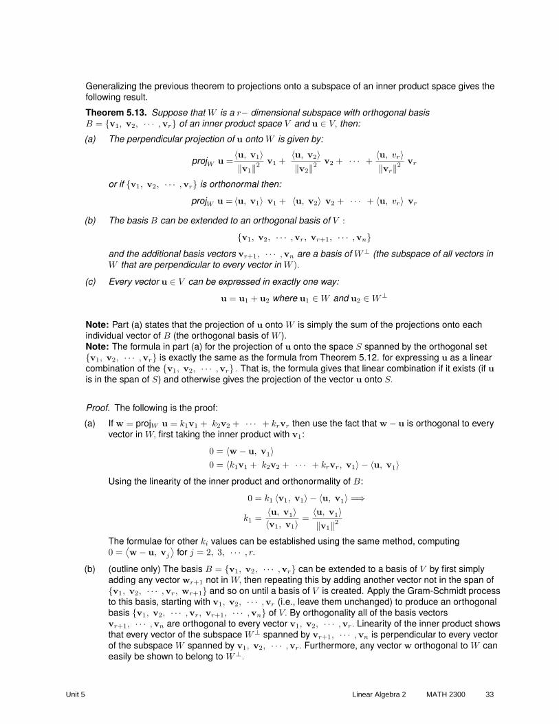
Example 5.6.7.Requires calculus. Compute the projection of the polynomial g (x) = x + x3 onto the subspace S ofP4, spanned by the first three Legendre polynomials:

f1 (x) = 1, f2 (x) = x, f3 (x) = x2 − 13

with the inner product defined by:

〈f, g〉 =∫ 1

−1

f (x) g (x) dx

Solution. It was shown in Example 5.6.4 that the set {f1, f2, f3} is orthogonal and spans the samesubspace as

{1, x, x2

}. Consequently, it is tempting to suppose that the projection of g (x) on S is the

polynomial x (that is, drop the x3 term). However, we will confirm this, or otherwise, using Theorem5.13.

According to Theorem 5.13, the projection is given by:

projS g =〈g, f1〉〈f1, f1〉 f1 (x) +

〈g, f2〉〈f2, f2〉 f2 (x) +

〈g, f3〉〈f3, f3〉f3 (x)

=

∫ 1

−1g (x) f1 (x) dx

∫ 1

−1(f1 (x))2 dx

f1 (x) +

∫ 1

−1g (x) f2 (x) dx

∫ 1

−1(f2 (x))2 dx

f2 (x) +

∫ 1

−1g (x) f3 (x) dx

∫ 1

−1(f3 (x))2 dx

f3 (x)

=

∫ 1

−1

(x + x3

)dx

∫ 1

−11 dx

× 1 +

∫ 1

−1

(x + x3

)xdx

∫ 1

−1x2 dx

x +

∫ 1

−1

(x + x3

) (x2 − 1

3

)dx

∫ 1

−1

(x2 − 1

3

)2dx

(x2 − 1

3

)

=02

+

(1615

)(

23

) x +0(845

)(

x2 − 13

)

projS g =85

x

Note: The intuitive argument above, that projS g = x, is clearly wrong. This is because the projection ofthe term x3 of g (x) onto S is not zero, but is in fact the polynomial 3

5x (check this for yourself). Sincethe other term in g (x) is x, and this is already in S, it follows that the projection of g onto S is35x + x = 8

5 x as was found above.

5.6.3 The QR− factorization of a matrixThe Gram-Schmidt Process takes a linearly independent set of vectors {u1, u2, u3, · · · , um} andconverts it into an orthogonal set {v1, v2, v3, · · · , vm} that spans the same vector space, that can bechanged to an orthonormal basis {w1, w2, w3, · · · , wm} by normalizing the vectors: wj = 1

‖vj‖vj .

This process can be expressed as a matrix factorization, A = QR, called the QR− factorization orQR− decomposition, of the matrix A. In this factorization the columns of A are the vectors uj , and thecolumns of Q are the normalized vectors wj . The matrix R is upper triangular (entries below the maindiagonal are zero), and each non-zero row i, column j entry is equal to the inner product of the form〈wi, uj〉 . In fact the whole Gram-Schmidt orthogonalization process can be carried out very efficientlyby working with matrices, rather than vectors.

The QR− factorization is usually applied to Euclidean spaces Rn, and the components of the vectorsui are written as columns of the matrix A. Similarly the wi components are columns of Q. In this case,if the number of vectors m = n, the dimension of the vector space, then the matrix Q will be an n× northogonal matrix. However, the matrix form applies to any inner product space.

Examples 5.6.8 and 5.6.9 show the QR− factorization in a simple two-vector case previously examinedin example 5.6.1. The complete result is given in Theorem 5.14.


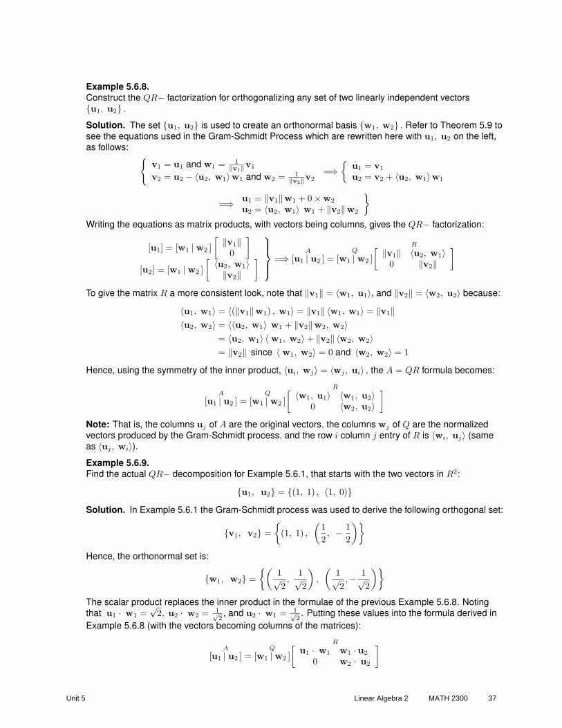
Example 5.6.8.Construct the QR− factorization for orthogonalizing any set of two linearly independent vectors{u1, u2} .

Solution. The set {u1, u2} is used to create an orthonormal basis {w1, w2} . Refer to Theorem 5.9 tosee the equations used in the Gram-Schmidt Process which are rewritten here with u1, u2 on the left,as follows:

{v1 = u1 and w1 = 1

‖v1‖v1

v2 = u2 − 〈u2, w1〉w1 and w2 = 1‖v2‖v2

=⇒{

u1 = v1

u2 = v2 + 〈u2, w1〉w1

=⇒ u1 = ‖v1‖w1 + 0×w2

u2 = 〈u2, w1〉 w1 + ‖v2‖w2

}

Writing the equations as matrix products, with vectors being columns, gives the QR− factorization:

[u1] = [w1 | w2 ][ ‖v1‖

0

]

[u2] = [w1 | w2 ][ 〈u2, w1〉

‖v2‖]

=⇒A

[u1 | u2 ] =Q

[w1 | w2 ]

R[ ‖v1‖ 〈u2, w1〉0 ‖v2‖

]

To give the matrix R a more consistent look, note that ‖v1‖ = 〈w1, u1〉, and ‖v2‖ = 〈w2, u2〉 because:

〈u1, w1〉 = 〈(‖v1‖w1) , w1〉 = ‖v1‖ 〈w1, w1〉 = ‖v1‖〈u2, w2〉 = 〈〈u2, w1〉 w1 + ‖v2‖w2, w2〉

= 〈u2, w1〉〈 w1, w2〉+ ‖v2‖ 〈w2, w2〉= ‖v2‖ since 〈 w1, w2〉 = 0 and 〈w2, w2〉 = 1

Hence, using the symmetry of the inner product, 〈ui, wj〉 = 〈wj , ui〉 , the A = QR formula becomes:

A

[u1 | u2 ] =Q

[w1 | w2 ]

R[ 〈w1, u1〉〈w1, u2〉0 〈w2, u2〉

]

Note: That is, the columns uj of A are the original vectors, the columns wj of Q are the normalizedvectors produced by the Gram-Schmidt process, and the row i column j entry of R is 〈wi, uj〉 (sameas 〈uj , wi〉).Example 5.6.9.Find the actual QR− decomposition for Example 5.6.1, that starts with the two vectors in R2:

{u1, u2} = {(1, 1) , (1, 0)}Solution. In Example 5.6.1 the Gram-Schmidt process was used to derive the following orthogonal set:

{v1, v2} ={

(1, 1) ,

(12, − 1

2

)}

Hence, the orthonormal set is:

{w1, w2} ={(

1√2,

1√2

),

(1√2,− 1√

2

)}

The scalar product replaces the inner product in the formulae of the previous Example 5.6.8. Notingthat u1 · w1 =

√2, u2 · w2 = 1√

2, and u2 · w1 = 1√

2. Putting these values into the formula derived in

Example 5.6.8 (with the vectors becoming columns of the matrices):

A

[u1 | u2 ] =Q

[w1 | w2 ]

R[u1 · w1 w1 · u2

0 w2 · u2

]


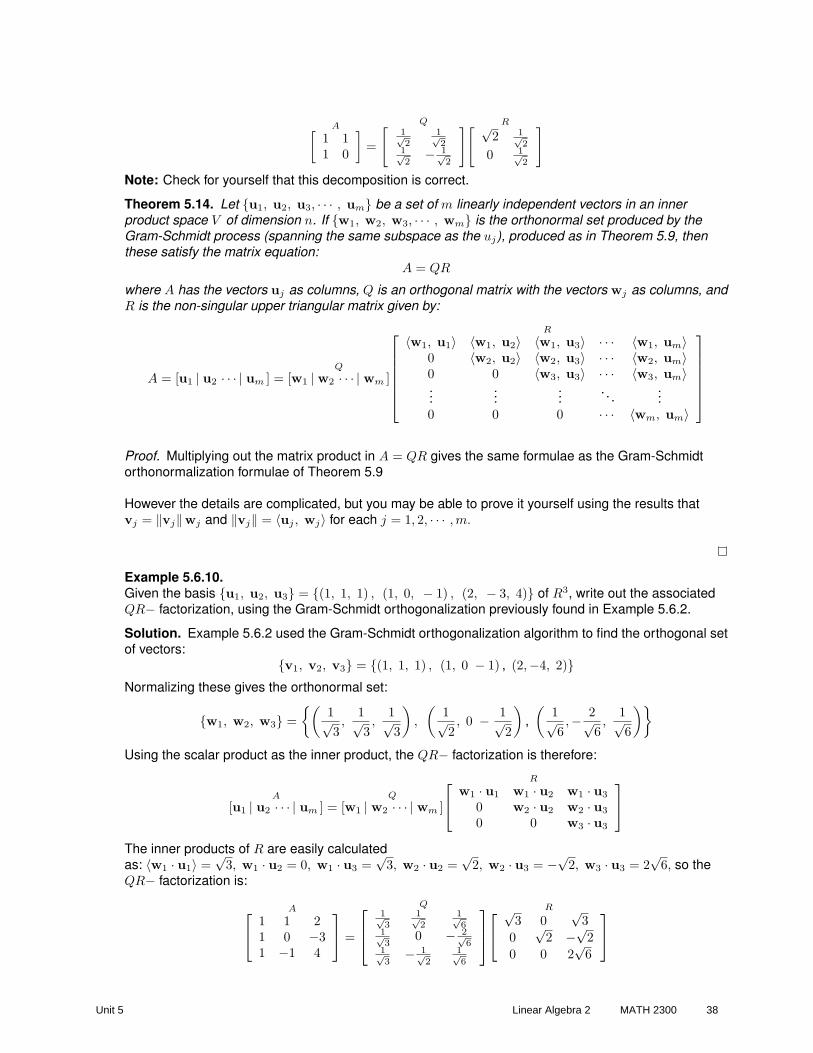
A[1 11 0

]=

Q[1√2

1√2

1√2

− 1√2

] R[ √2 1√

2

0 1√2

]

Note: Check for yourself that this decomposition is correct.

Theorem 5.14. Let {u1, u2, u3, · · · , um} be a set of m linearly independent vectors in an innerproduct space V of dimension n. If {w1, w2, w3, · · · , wm} is the orthonormal set produced by theGram-Schmidt process (spanning the same subspace as the uj), produced as in Theorem 5.9, thenthese satisfy the matrix equation:

A = QR

where A has the vectors uj as columns, Q is an orthogonal matrix with the vectors wj as columns, andR is the non-singular upper triangular matrix given by:

A = [u1 | u2 · · · | um ] =Q

[w1 | w2 · · · | wm ]

R

〈w1, u1〉〈w1, u2〉〈w1, u3〉 · · · 〈w1, um〉0 〈w2, u2〉〈w2, u3〉 · · · 〈w2, um〉0 0 〈w3, u3〉 · · · 〈w3, um〉...

......

. . ....

0 0 0 · · · 〈wm, um〉

Proof. Multiplying out the matrix product in A = QR gives the same formulae as the Gram-Schmidtorthonormalization formulae of Theorem 5.9

However the details are complicated, but you may be able to prove it yourself using the results thatvj = ‖vj‖wj and ‖vj‖ = 〈uj , wj〉 for each j = 1, 2, · · · ,m.

Example 5.6.10.Given the basis {u1, u2, u3} = {(1, 1, 1) , (1, 0, − 1) , (2, − 3, 4)} of R3, write out the associatedQR− factorization, using the Gram-Schmidt orthogonalization previously found in Example 5.6.2.

Solution. Example 5.6.2 used the Gram-Schmidt orthogonalization algorithm to find the orthogonal setof vectors:

{v1, v2, v3} = {(1, 1, 1) , (1, 0 − 1) , (2,−4, 2)}Normalizing these gives the orthonormal set:

{w1, w2, w3} ={(

1√3,

1√3,

1√3

),

(1√2, 0 − 1√

2

),

(1√6,− 2√

6,

1√6

)}

Using the scalar product as the inner product, the QR− factorization is therefore:

A

[u1 | u2 · · · | um ] =Q

[w1 | w2 · · · | wm ]

R

w1 · u1 w1 · u2 w1 · u3

0 w2 · u2 w2 · u3

0 0 w3 · u3

The inner products of R are easily calculatedas: 〈w1 · u1〉 =

√3, w1 · u2 = 0, w1 · u3 =

√3, w2 · u2 =

√2, w2 · u3 = −√2, w3 · u3 = 2

√6, so the

QR− factorization is:

A

1 1 21 0 −31 −1 4

=

Q

1√3

1√2

1√6

1√3

0 − 2√6

1√3

− 1√2

1√6

R√

3 0√

30

√2 −√2

0 0 2√

6


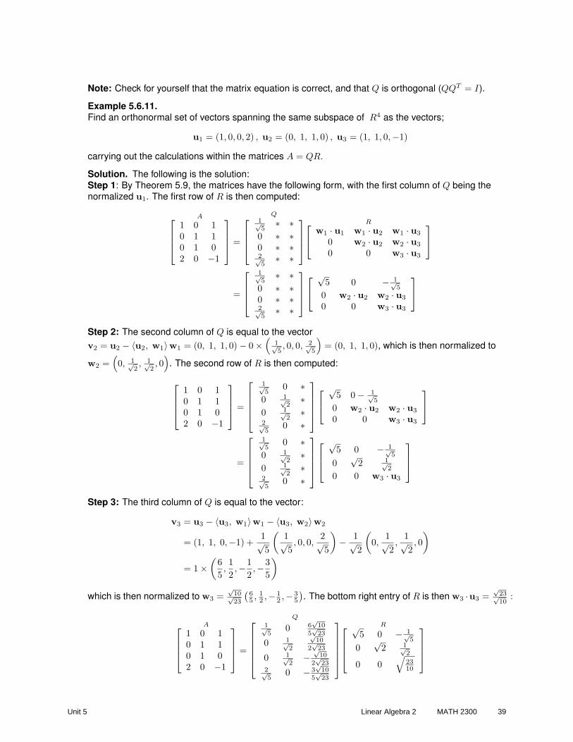
Note: Check for yourself that the matrix equation is correct, and that Q is orthogonal (QQT = I).

Example 5.6.11.Find an orthonormal set of vectors spanning the same subspace of R4 as the vectors;

u1 = (1, 0, 0, 2) , u2 = (0, 1, 1, 0) , u3 = (1, 1, 0,−1)

carrying out the calculations within the matrices A = QR.

Solution. The following is the solution:Step 1: By Theorem 5.9, the matrices have the following form, with the first column of Q being thenormalized u1. The first row of R is then computed:

A

1 0 10 1 10 1 02 0 −1

=

Q

1√5

∗ ∗0 ∗ ∗0 ∗ ∗2√5

∗ ∗

R

w1 · u1 w1 · u2 w1 · u3

0 w2 · u2 w2 · u3

0 0 w3 · u3

=

1√5

∗ ∗0 ∗ ∗0 ∗ ∗2√5

∗ ∗

√

5 0 − 1√5

0 w2 · u2 w2 · u3

0 0 w3 · u3

Step 2: The second column of Q is equal to the vectorv2 = u2 − 〈u2, w1〉w1 = (0, 1, 1, 0)− 0×

(1√5, 0, 0, 2√

5

)= (0, 1, 1, 0), which is then normalized to

w2 =(0, 1√

2, 1√

2, 0

). The second row of R is then computed:

1 0 10 1 10 1 02 0 −1

=

1√5

0 ∗0 1√

2∗

0 1√2

∗2√5

0 ∗

√

5 0− 1√5

0 w2 · u2 w2 · u3

0 0 w3 · u3

=

1√5

0 ∗0 1√

2∗

0 1√2

∗2√5

0 ∗

√5 0 − 1√

5

0√

2 1√2

0 0 w3 · u3

Step 3: The third column of Q is equal to the vector:

v3 = u3 − 〈u3, w1〉w1 − 〈u3, w2〉w2

= (1, 1, 0,−1) +1√5

(1√5, 0, 0,

2√5

)− 1√

2

(0,

1√2,

1√2, 0

)

= 1×(

65,12,−1

2,−3

5

)

which is then normalized to w3 =√

10√23

(65 , 1

2 ,− 12 ,− 3

5

). The bottom right entry of R is then w3 ·u3 =

√23√10

:

A

1 0 10 1 10 1 02 0 −1

=

Q

1√5

0 6√

105√

23

0 1√2

√10

2√

23

0 1√2

−√

102√

232√5

0 − 3√

105√

23

R

√5 0 − 1√

5

0√

2 1√2

0 0√

2310


Note: Verify for yourself that the matrix equation is correct.Note: Some authors make Q into an orthogonal matrix by adding appropriate extra columns (one isneeded in this case), and by adding rows of zeros to the bottom of R to make the matrix multiplicationcompatible. The extra column of Q is found by choosing an arbitrary fourth vector u4 (it is very unlikelyto be in the span of {u1,u2,u3}) and then continuing the Gram-Schmidt algorithm for one more step,but leaving out the extra column in the final matrix equation. This form of the factorization in thisexample is:

A

1 0 10 1 10 1 02 0 −1

=

Q

1√5

0 6√

105√

232√23

0 1√2

√10

2√

23− 3√

23

0 1√2

−√

102√

233√23

2√5

0 − 3√

105√

23− 1√

23

R

√5 0 − 1√

5

0√

2 1√2

0 0√

2310

0 0 0

For completeness we give a QR− factorization for P3, but in fact this matrix factorization is rarely usedoutside of Euclidean spaces.

Example 5.6.12.Referring to Example 5.6.3, starting with the polynomials{g1 (x) , g2 (x) , g3 (x) , g4 (x)} =

{1, 1 + x, 1− 2x2, x + x3

}and inner product defined by:

⟨a0 + a1x + a2x

2 + a3x3, b0 + b1x + b2x

2 + b3x3⟩

= a0b0 + a1b1 + a2b2 + a3b3

write the Gram-Schmidt orthogonalization as a QR− factorization.

Solution. The orthogonal set found in Example 5.6.3 is:

{f1 (x) , f2 (x) , f3 (x) , f4 (x)} ={1, x, − 2x2, x3

}

Normalizing these gives the orthonormal basis of P3 :

{h1 (x) , h2 (x) , h3 (x) , h4 (x)} ={1, x, x2, x3

}

The QR− factorization is therefore:[

g1 (x) g2 (x) g3 (x) g4 (x)]

=

[h1 (x) h2 (x) h3 (x) h4 (x)

]

〈h1, g1〉〈h1, g2〉〈h1, g3〉〈h1, g4〉0 〈h2, g2〉〈h2, g3〉〈h2, g4〉0 0 〈h3, g3〉〈h3, g4〉0 0 0 〈h4, g4〉

and 〈h1, g1〉 = 1, 〈h1, g2〉 = 1, 〈h1, g3〉 = 1 〈h1, g3〉 = 0, 〈h2, g2〉 = 1, 〈h2, g3〉 = 0, 〈h2, g3〉 = 1,〈h3, g3〉 = −2, 〈h3, g4〉 = 0, 〈h4, g4〉 = 1, so

A[1 1 + x 1− 2x2 x + x3

]=

Q[1 x x2 x3

]R

1 1 1 00 1 0 10 0 −2 00 0 0 1

Note: Check for yourself that the matrix equality is correct.



1. Let S be the subspace of R3 spanned by the following set of two vectors:

{(1, 2, − 1) , (3, 0, 3)}

(a) Check that the set of vectors is orthogonal.

(b) Convert it to an orthonormal set.

(c) Extend it to an orthonormal basis of R3 (Hint: add to the two orthogonal vectors any othervector not in S - a random choice usually works - and apply one step of the Gram-Schmidtprocess).

(d) Find the projection of the vector (1, 2, 3) onto S (use Theorem 5.13).

2. For the following set of vectors in R3 :

{(1, 2, 0) , (1, 1, 1) , (3, − 2, 1)}

(a) Use the Gram-Schmidt process of Theorem 5.8 to find an orthogonal basis of R3.

(b) Find an orthonormal basis of R3.

(c) Can you be certain that the original three vectors are linearly independent?

3. Apply the Gram-Schmidt orthogonalization process (Theorem 5.8) to the following set of vectorsin R4. What do you conclude about this set?

{(1, 2, 0, − 3) , (1, 1, 1, 1) , (1, 0, 2, 5)}

4. For the following set of vectors in R3 :

{(1, 0, − 1) , (1, 1, 0) , (1, 1, 1)}

(a) Use the Gram-Schmidt process of Theorem 5.8 to find an orthonormal basis of R3.

(b) Use the Gram-Schmidt process of Theorem 5.9 to find an orthonormal basis of R3. Discusswhich of the two methods in (a) and (b) is easiest.

(c) Use Theorem 5.12 to find linear combination of the basis vectors, giving the two vectorsu1 = (1, 3,−2) , u2 = (4, 0, 1).

(d) Show that Theorem 5.11 gives the correct values for u1 · u2, for the norms of u1. and u2, andfor the distance between u1 and u2.

5. The following set of polynomials is a basis of P2:{1− x2, x + 2x2, − 2 + x + 3x2

}

(a) Find an orthogonal basis using the Gram-Schmidt orthogonalization process (Theorem 5.8)with the inner product of Example 5.6.3 (scalar product of the vectors of coefficients).

(b) Find an orthogonal basis using the Gram-Schmidt orthogonalization process (Theorem 5.8)with the inner product:

⟨a0 + a1x + a2x

2, b0 + b1x + b2x2⟩

= a0b0 + 2a1b1 + 3a2b2

(c) Requires calculus and more difficult. Find an orthogonal basis using the Gram-Schmidtorthogonalization process (Theorem 5.8) with the inner product of Example 5.6.7 (theintegral of the product from x = −1 to x = 1).

(d) Find orthonormal basis with the inner product of part (a).

(e) Find orthonormal basis with the inner product of part (b).


6. For the basis vectors found in the previous question

(a) Express the polynomial 2 + 3x− 4x2 as a linear combination of the orthogonal polynomialsfound in part (a) of the previous question (see Theorems 5.11and 5.12).

(b) Express the polynomial 2 + 3x− 4x2 as a linear combination of the orthogonal polynomialsfound in part (b)of the previous question.

(c) Express the Gram-Schmidt process covered in part (a) and (d) of the previous question as aQR− factorization.

7. Apply the Gram-Schmidt orthogonalization process (Theorem 5.8) with the inner product ofExample 5.6.3 (scalar product of the vectors of coefficients).to the set of polynomials in P3

{1− x2, x + 2x2, − 2 + x + 4x2

}

What do you conclude?

8. Let S be the subspace of M22 spanned by the three matrices:

S ={[

1 3−2 0

],

[2 12 1

],

[0 32 1

]}

(a) Find an orthogonal basis of S using the Gram-Schmidt orthogonalization process (Theorem5.8) with the inner product of Example 5.6.6 (scalar product of the 4−vectors formed by theentries of the matrices).

(b) Find an orthonormal basis of S.

(c) Attempt to express the following matrix as a linear combination of the orthonormal basismatrices of S (see Theorems 5.11 and 5.12):

[5 20 1

]

(d) Attempt to express the following matrix as a linear combination of the orthonormal basismatrices of S : [

3 0−1 2

]

9. Requires calculus and is more difficult. Starting with the following five basis polynomials of P4

and the inner product 〈f, g〉 =∫ 1

−1f (x) g (x) dx :

{1, x, x2, x3, x4

}

(a) Use the Gram-Schmidt orthogonalization process (Theorem 5.8) to find the fifth function ofthe orthogonal basis (the first four are given in Example 5.6.4).Note: These orthogonal basis polynomials are multiples of the first four LegendrePolynomials that are very useful in some Engineering applications.

(b) Convert the basis from part (a) into an orthonormal basis of P4.

10. Let W be the subspace of R4 spanned by the two vectors:

{(1, 0, 0, 1) , (1, 2, 0, 1)}(a) Find a basis of W⊥.

(b) If u = (2, 3, 0, 4) then find two (unique) vectors u1 ∈ W, u2 ∈ W⊥ such that u = u1 + u2.

(c) Find the QR− factorization equivalent to the Gram-Schmidt process in part (a) (that is,including all four basis vectors of W and W⊥).


11. Find, if possible, the QR− factorization of the following matrices:

(a) A =[

1 30 4

], (b) B =

1 1 00 1 11 −1 1

, (c) C =

3 54 00 −2

, (d) D =

1 0 20 1 32 −1 1

Solutions

1. For the vectors (1, 2, − 1) , (3, 0, 3) :

(a) They are orthogonal since (1, 2, − 1) · (3, 0, 3) = 1× 3 + 2× 0 + (−1)× 3 = 0.

(b) Normalizing (dividing the vector by its norm/length) the vectors gives the orthonormal set:

w1 =(

1√6,

2√6, − 1√

6

), w2 =

(1√2, 0,

1√2

)

(c) Choose, randomly, the vector u = (1, 0, 0) and apply the last step of the Gram-Schmidtalgorithm (Theorem 5.9) to the vector {w1,w2,u} to form an orthonormal set {w1,w2,w3}using the intermediate vector v :

v= u− (w1 · u)w1 − (w2 · u)w2

= (1, 0, 0)− 1√6

(1√6,

2√6, − 1√

6

)− 1√

2

(1√2, 0,

1√2

)

= (1, 0, 0)−(

16,

13, − 1

6

)−

(12, 0,

12

)

v =(

13, − 1

3, − 1

3

)

Normalizing v gives the required result w3 =(

1√3, − 1√

3, − 1√

3

)and the orthonormal

basis:

w1 =(

1√6,

2√6, − 1√

6

), w2 =

(1√2, 0,

1√2

), w3 =

(1√3, − 1√

3, − 1√

3

)

(d) The projection of the vector u = (1, 2, 3) onto the subspace S with orthonormal basis{w1, w2} is given by (see Theorem 5.13):

projS u= 〈u, w1〉 w1 + 〈u, w2〉 w2

=[(1, 2, 3) ·

(1√6,

2√6, − 1√

6

)]w1 +

[(1, 2, 3) ·

(1√2, 0,

1√2

)]w2

=13

√6

(1√6,

2√6, − 1√

6

)+ 2

√2

(1√2, 0,

1√2

)

=(

13,

23, − 1

3

)+ (2, 0, 2)

projS u =(

73,

23,

53

)

2. For the vectors:u1 = (1, 2, 0) , u2 = (1, 1, 0) , u3 = (3, − 2, 1)


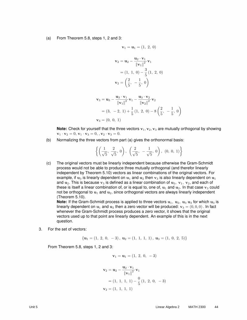
(a) From Theorem 5.8, steps 1, 2 and 3:

v1 = u1 = (1, 2, 0)

v2 = u2 − u2 · v1

‖v1‖2v1

= (1, 1, 0)− 35

(1, 2, 0)

v2 =(

25, − 1

5, 0

)

v3 = u3 − u3 · v1

‖v1‖2v1 − u3 · v2

‖v2‖2v2

= (3, − 2, 1) +15

(1, 2, 0)− 8(

25, − 1

5, 0

)

v3 = (0, 0, 1)

Note: Check for yourself that the three vectors v1,v2,v3 are mutually orthogonal by showingv1 · v2 = 0, v1 · v3 = 0, ,v2 · v3 = 0.

(b) Normalizing the three vectors from part (a) gives the orthonormal basis:{(

1√5,

2√5, 0

),

(2√5, − 1√

5, 0

), (0, 0, 1)

}

(c) The original vectors must be linearly independent because otherwise the Gram-Schmidtprocess would not be able to produce three mutually orthogonal (and therefor linearlyindependent by Theorem 5.10) vectors as linear combinations of the original vectors. Forexample, if u3 is linearly dependent on u1 and u2 then v3 is also linearly dependent on u1

and u2. This is because v3 is defined as a linear combination of u3, v1, v2, and each ofthese is itself a linear combination of, or is equal to, one of, u1 and u2. In that case v3 couldnot be orthogonal to u1 and u2, since orthogonal vectors are always linearly independent(Theorem 5.10).Note: If the Gram-Schmidt process is applied to three vectors u1, u2, u3 u3 for which u3 islinearly dependent on u1 and u2 then a zero vector will be produced: v3 = (0, 0, 0) . In factwhenever the Gram-Schmidt process produces a zero vector, it shows that the originalvectors used up to that point are linearly dependent. An example of this is in the nextquestion.

3. For the set of vectors:

{u1 = (1, 2, 0, − 3) , u2 = (1, 1, 1, 1) , u3 = (1, 0, 2, 5)}

From Theorem 5.8, steps 1, 2 and 3:

v1 = u1 = (1, 2, 0, − 3)

v2 = u2 − u2 · v1

‖v1‖2v1

= (1, 1, 1, 1)− 05

(1, 2, 0, − 3)

v2 = (1, 1, 1, 1)


That is v2 = u2 because u2 was already orthogonal to v1. Finally,

v3 = u3 − u3 · v1

‖v1‖2v1 − u3 · v2

‖v2‖2v2

= (1, 0, 2, 5) +1414

(1, 2, 0,−3)− 84

(1, 1, 1, 1)

= (1, 0, 2, 5) + (1, 2, 0,−3)− (2, 2, 2, 2)v3 = (0, 0, 0, 0)

Hence, v3 = 0, the zero vector, and this indicates that it is not possible to find a non-zero vectororthogonal to v1 and v2. This only happens when the original set of vectors is linearly dependent.Note: Check for yourself that the linear dependence is: u3 = 2u2 − u1.

4. For the vectors:u1 = (1, 0, − 1) , u2 = (1, 1, 0) , u3 = (1, 2, − 1)

(a) From Theorem 5.8, steps 1, 2 and 3:

v1 = u1 = (1, 0, − 1)

v2 = u2 − u2 · v1

‖v1‖2v1

= (1, 1, 0)− 12

(1, 0, − 1)

v2 =(

12, 1,

12

)

v3 = u3 − u3 · v1

‖v1‖2v1 − u3 · v2

‖v2‖2v2

= (1, 2, − 1)− 22

(1, 0, − 1)− 2(32

)(

12, 1,

12

)

v3 =(−2

3,

23, − 2

3

)

Hence, simplifying by multiplying two of the vectors by an appropriate constant, anorthogonal set is:

{v1, 2v2, − 3

2v3

}= {(1, 0, − 1) , (1, 2, 1) , (1, − 1, 1)}

Hence, normalizing the vectors gives the orthonormal set:

{w1, w2, w3} ={(

1√2, 0, − 1√

2

),

(1√6,

2√6,

1√6

),

(1√3, − 1√

3,

1√3

)}

{w1, w2, w3} ={

1√2

(1, 0,−1) ,1√6

(1, 2, 1) ,1√3

(1,−1, 1)}

(b) Repeat the process, using Theorem 5.9, steps 1, 2 and 3, starting with the vectorsu1 = (1, 0, − 1) , u2 = (1, 1, 0) , u3 = (1, 2, − 1) :

w1 =1

‖u1‖u1 =(

1√2, 0, − 1√

2

)


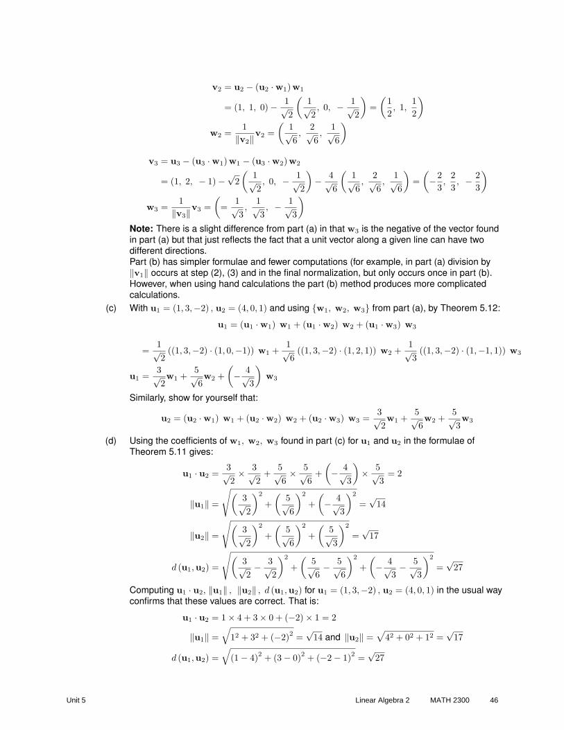
v2 = u2 − (u2 ·w1)w1

= (1, 1, 0)− 1√2

(1√2, 0, − 1√

2

)=

(12, 1,

12

)

w2 =1

‖v2‖v2 =(

1√6,

2√6,

1√6

)

v3 = u3 − (u3 ·w1)w1 − (u3 ·w2)w2

= (1, 2, − 1)−√

2(

1√2, 0, − 1√

2

)− 4√

6

(1√6,

2√6,

1√6

)=

(−2

3,

23, − 2

3

)

w3 =1

‖v3‖v3 =(

=1√3,

1√3, − 1√

3

)

Note: There is a slight difference from part (a) in that w3 is the negative of the vector foundin part (a) but that just reflects the fact that a unit vector along a given line can have twodifferent directions.Part (b) has simpler formulae and fewer computations (for example, in part (a) division by‖v1‖ occurs at step (2), (3) and in the final normalization, but only occurs once in part (b).However, when using hand calculations the part (b) method produces more complicatedcalculations.

(c) With u1 = (1, 3,−2) , u2 = (4, 0, 1) and using {w1, w2, w3} from part (a), by Theorem 5.12:

u1 = (u1 ·w1) w1 + (u1 ·w2) w2 + (u1 ·w3) w3

=1√2

((1, 3,−2) · (1, 0,−1)) w1 +1√6

((1, 3,−2) · (1, 2, 1)) w2 +1√3

((1, 3,−2) · (1,−1, 1)) w3

u1 =3√2w1 +

5√6w2 +

(− 4√

3

)w3

Similarly, show for yourself that:

u2 = (u2 ·w1) w1 + (u2 ·w2) w2 + (u2 ·w3) w3 =3√2w1 +

5√6w2 +

5√3w3

(d) Using the coefficients of w1, w2, w3 found in part (c) for u1 and u2 in the formulae ofTheorem 5.11 gives:

u1 · u2 =3√2× 3√

2+

5√6× 5√

6+

(− 4√

3

)× 5√

3= 2

‖u1‖ =

√(3√2

)2

+(

5√6

)2

+(− 4√

3

)2

=√

14

‖u2‖ =

√(3√2

)2

+(

5√6

)2

+(

5√3

)2

=√

17

d (u1,u2) =

√(3√2− 3√

2

)2

+(

5√6− 5√

6

)2

+(− 4√

3− 5√

3

)2

=√

27

Computing u1 · u2, ‖u1‖ , ‖u2‖ , d (u1,u2) for u1 = (1, 3,−2) , u2 = (4, 0, 1) in the usual wayconfirms that these values are correct. That is:

u1 · u2 = 1× 4 + 3× 0 + (−2)× 1 = 2

‖u1‖ =√

12 + 32 + (−2)2 =√

14 and ‖u2‖ =√

42 + 02 + 12 =√

17

d (u1,u2) =√

(1− 4)2 + (3− 0)2 + (−2− 1)2 =√

27


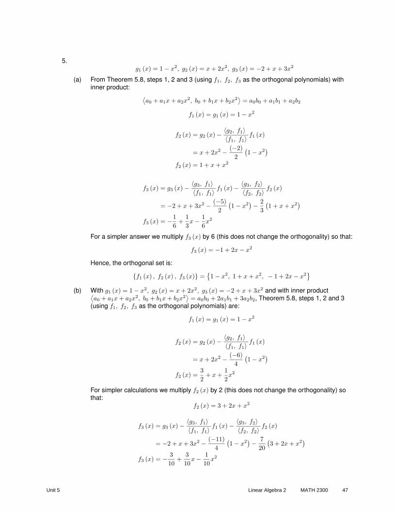
5.g1 (x) = 1− x2, g2 (x) = x + 2x2, g3 (x) = −2 + x + 3x2

(a) From Theorem 5.8, steps 1, 2 and 3 (using f1, f2, f3 as the orthogonal polynomials) withinner product:

⟨a0 + a1x + a2x

2, b0 + b1x + b2x2⟩

= a0b0 + a1b1 + a2b2

f1 (x) = g1 (x) = 1− x2

f2 (x) = g2 (x)− 〈g2, f1〉〈f1, f1〉 f1 (x)

= x + 2x2 − (−2)2

(1− x2

)

f2 (x) = 1 + x + x2

f3 (x) = g3 (x)− 〈g3, f1〉〈f1, f1〉 f1 (x)− 〈g3, f2〉

〈f2, f2〉 f2 (x)

= −2 + x + 3x2 − (−5)2

(1− x2

)− 23

(1 + x + x2

)

f3 (x) = −16

+13x− 1

6x2

For a simpler answer we multiply f3 (x) by 6 (this does not change the orthogonality) so that:

f3 (x) = −1 + 2x− x2

Hence, the orthogonal set is:

{f1 (x) , f2 (x) , f3 (x)} ={1− x2, 1 + x + x2, − 1 + 2x− x2

}

(b) With g1 (x) = 1− x2, g2 (x) = x + 2x2, g3 (x) = −2 + x + 3x2 and with inner product⟨a0 + a1x + a2x

2, b0 + b1x + b2x2⟩

= a0b0 + 2a1b1 + 3a2b2, Theorem 5.8, steps 1, 2 and 3(using f1, f2, f3 as the orthogonal polynomials) are:

f1 (x) = g1 (x) = 1− x2

f2 (x) = g2 (x)− 〈g2, f1〉〈f1, f1〉 f1 (x)

= x + 2x2 − (−6)4

(1− x2

)

f2 (x) =32

+ x +12x2

For simpler calculations we multiply f2 (x) by 2 (this does not change the orthogonality) sothat:

f2 (x) = 3 + 2x + x2

f3 (x) = g3 (x)− 〈g3, f1〉〈f1, f1〉 f1 (x)− 〈g3, f2〉

〈f2, f2〉 f2 (x)

= −2 + x + 3x2 − (−11)4

(1− x2

)− 720

(3 + 2x + x2

)

f3 (x) = − 310

+310

x− 110

x2


For a simpler answer we multiply f2 (x) by 2 (this does not change the orthogonality) so that:

f3 (x) = −3 + 3x− x2


{f1 (x) , f2 (x) , f3 (x)} ={1− x2, 3 + 2x + x2, − 3 + 3x− x2

}

Note: Check for yourself that these three polynomials are mutually orthogonal but only forthe inner product

⟨a0 + a1x + a2x

2, b0 + b1x + b2x2⟩

= a0b0 + 2a1b1 + 3a2b2.

(c) With g1 (x) = 1− x2, g2 (x) = x + 2x2, g3 (x) = −2 + x + 3x2 and with inner product〈p (x) , q (x)〉 =

∫ 1

−1p (x) q (x) dx, Theorem 5.8, steps 1, 2 and 3, using f1, f2, f3 as the

orthogonal polynomials, and omitting details of the integrations, are:

f1 (x) = g1 (x) = 1− x2

f2 (x) = g2 (x)− 〈g2, f1〉〈f1, f1〉 f1 (x)

= x + 2x2 −∫ 1

−1

(x + 2x2

) (1− x2

)dx

∫ 1

−1(1− x2)2 dx

(1− x2

)

= x + 2x2 −(

815

)(

1615

) (1− x2

)

f2 (x) = −12

+ x +52x2

For simpler calculations we multiply f2 (x) by 2 (this does not change the orthogonality) sothat:

f2 (x) = −1 + 2x + 5x2

f3 (x) = g3 (x)− 〈g3, f1〉〈f1, f1〉 f1 (x)− 〈g3, f2〉

〈f2, f2〉 f2 (x)

= −2 + x + 3x2 −∫ 1

−1

(−2 + x + 3x2) (

1− x2)

dx∫ 1

−1(1− x2)2 dx

(1− x2

)

−∫ 1

−1

(−2 + x + 3x2) (−1 + 2x + 5x2

)dx

∫ 1

−1(−1 + 2x + 5x2)2 dx

(−1 + 2x + 5x2)

= −2 + x + 3x2 −(− 28

15

)(

1615

) (1− x2

)−(

83

)

8(−1 + 2x + 5x2

)

f3 (x) =112

+13x− 5

12x2

For a simpler answer we multiply f3 (x) by 12 (this does not change the orthogonality) sothat:

f3 (x) = 1 + 4x− 5x2


{f1 (x) , f2 (x) , f3 (x)} ={1− x2, − 1 + 2x + 5x2, 1 + 4x− 5x2

}

Note: Check for yourself that these three polynomials are mutually orthogonal but only forthe inner product used in this part.


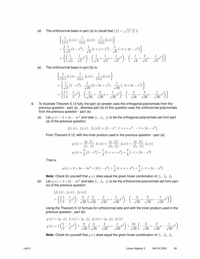
(d) The orthonormal basis in part (a) is (recall that ‖f‖ =√〈f, f〉 ):

{1

‖f1‖f1 (x) ,1

‖f2‖ f2 (x) ,1

‖f3‖f3 (x)}

={

1√2

(1− x2

),

1√3

(1 + x + x2

),

1√6

(−1 + 2x− x2)}

={(

1√2− 1√

2x2

),

(1√3

+1√3x +

1√3x2

),

(− 1√

6+

2√6x− 1√

6x2

)}

(e) The orthonormal basis in part (b) is:{

1‖f1‖f1 (x) ,

1‖f2‖ f2 (x) ,

1‖f3‖f3 (x)

}

={

1√4

(1− x2

),

1√20

(3 + 2x + x2

),

1√30

(−3 + 3x− x2)}

={(

12− 1

2x2

),

(3√20

+2√20

x +1√20

x2

),

(− 3√

30+

3√30

x− 1√30

x2

)}

6. To illustrate Theorem 5.12 fully, the part (a) answer uses the orthogonal polynomials from theprevious question - part (a) , whereas part (b) of this question uses the orthonormal polynomialsfrom the previous question - part (e).

(a) Let g (x) = 2 + 3x− 4x2 and take f1, f2, f3 to be the orthogonal polynomials set from part(a) of the previous question:

{f1 (x) , f2 (x) , f3 (x)} ={1− x2, 1 + x + x2, − 1 + 2x− x2

}

From Theorem 5.12, with the inner product used in the previous question - part (a):

g (x) =〈g, f1〉〈f1, f1〉 f1 (x) +

〈g, f2〉〈f2, f2〉 f2 (x) +

〈g, f3〉〈f3, f3〉 f3 (x)

g (x) =62

(1− x2

)+

13

(1 + x + x2

)+

86

(−1 + 2x− x2)

That is,

g (x) = 2 + 3x− 4x2 = 3(1− x2

)+

13

(1 + x + x2

)+

43

(−1 + 2x− x2)

Note: Check for yourself that g (x) does equal the given linear combination of f1, f2, f3

(b) Let g (x) = 2 + 3x− 4x2 and take f1, f2, f3 to be the orthonormal polynomials set from part(e) of the previous question:

{f1 (x) , f2 (x) , f3 (x)}

={(

12− 1

2x2

),

6√20

(3√20

+2√20

x +1√20

x2

),

(− 3√

30+

3√30

x− 1√30

x2

)}

Using the Theorem 5.12 formula for orthonormal sets and with the inner product used in theprevious question - part (b):

g (x) = 〈g, f1〉 f1 (x) + 〈g, f2〉 f2 (x) + 〈g, f3〉 f3 (x)

g (x) = 7(

12− 1

2x2

)+

6√20

(3√20

+2√20

x +1√20

x2

)+

24√30

(− 3√

30+

3√30

x− 1√30

x2

)

Note: Check for yourself that g (x) does equal the given linear combination of f1, f2, f3.


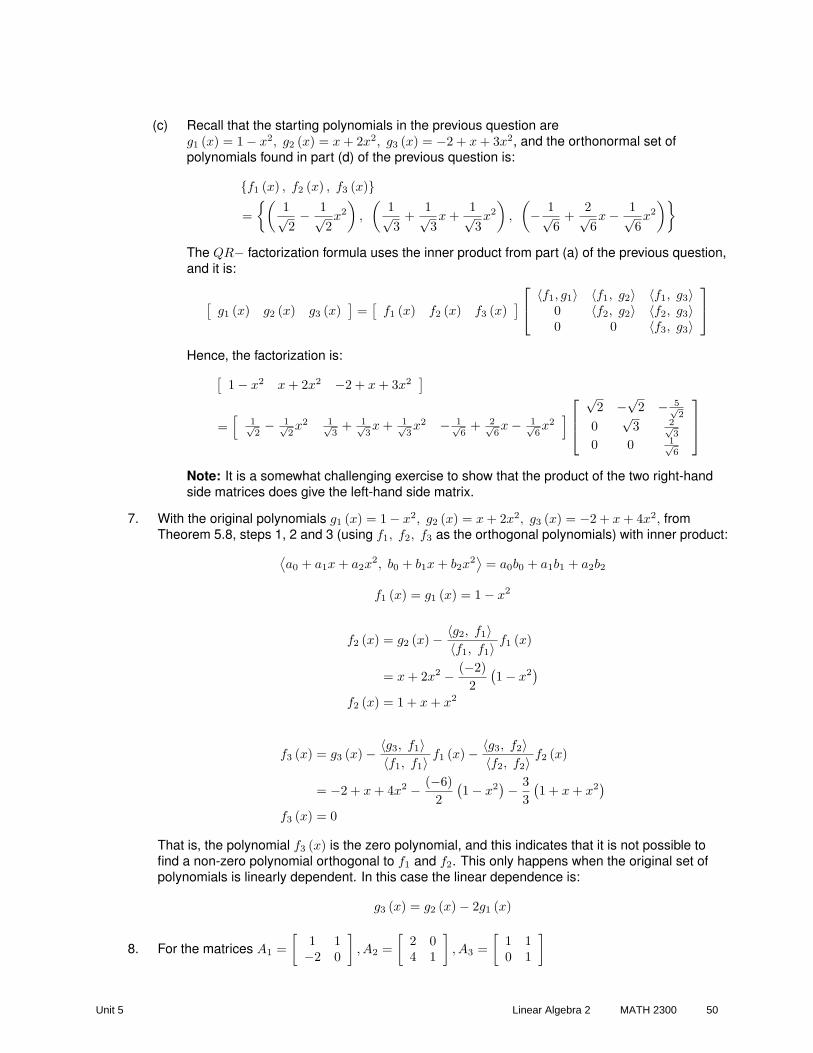
(c) Recall that the starting polynomials in the previous question areg1 (x) = 1− x2, g2 (x) = x + 2x2, g3 (x) = −2 + x + 3x2, and the orthonormal set ofpolynomials found in part (d) of the previous question is:

{f1 (x) , f2 (x) , f3 (x)}

={(

1√2− 1√

2x2

),

(1√3

+1√3x +

1√3x2

),

(− 1√

6+

2√6x− 1√

6x2

)}

The QR− factorization formula uses the inner product from part (a) of the previous question,and it is:

[g1 (x) g2 (x) g3 (x)

]=

[f1 (x) f2 (x) f3 (x)

]〈f1, g1〉〈f1, g2〉〈f1, g3〉

0 〈f2, g2〉〈f2, g3〉0 0 〈f3, g3〉

Hence, the factorization is:[

1− x2 x + 2x2 −2 + x + 3x2]

=[

1√2− 1√

2x2 1√

3+ 1√

3x + 1√

3x2 − 1√

6+ 2√

6x− 1√

6x2

]

√2 −√2 − 5√

2

0√

3 2√3

0 0 1√6

Note: It is a somewhat challenging exercise to show that the product of the two right-handside matrices does give the left-hand side matrix.

7. With the original polynomials g1 (x) = 1− x2, g2 (x) = x + 2x2, g3 (x) = −2 + x + 4x2, fromTheorem 5.8, steps 1, 2 and 3 (using f1, f2, f3 as the orthogonal polynomials) with inner product:

⟨a0 + a1x + a2x

2, b0 + b1x + b2x2⟩

= a0b0 + a1b1 + a2b2

f1 (x) = g1 (x) = 1− x2

f2 (x) = g2 (x)− 〈g2, f1〉〈f1, f1〉 f1 (x)

= x + 2x2 − (−2)2

(1− x2

)

f2 (x) = 1 + x + x2

f3 (x) = g3 (x)− 〈g3, f1〉〈f1, f1〉 f1 (x)− 〈g3, f2〉

〈f2, f2〉 f2 (x)

= −2 + x + 4x2 − (−6)2

(1− x2

)− 33

(1 + x + x2

)

f3 (x) = 0

That is, the polynomial f3 (x) is the zero polynomial, and this indicates that it is not possible tofind a non-zero polynomial orthogonal to f1 and f2. This only happens when the original set ofpolynomials is linearly dependent. In this case the linear dependence is:

g3 (x) = g2 (x)− 2g1 (x)

8. For the matrices A1 =[

1 1−2 0

], A2 =

[2 04 1

], A3 =

[1 10 1

]


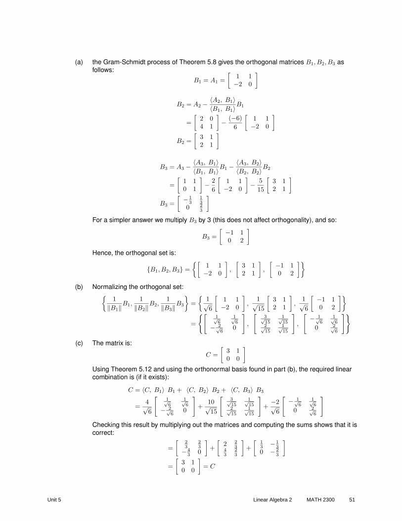
(a) the Gram-Schmidt process of Theorem 5.8 gives the orthogonal matrices B1, B2, B3 asfollows:

B1 = A1 =[

1 1−2 0

]

B2 = A2 − 〈A2, B1〉〈B1, B1〉B1

=[

2 04 1

]− (−6)

6

[1 1−2 0

]

B2 =[

3 12 1

]

B3 = A3 − 〈A3, B1〉〈B1, B1〉B1 − 〈A3, B2〉

〈B2, B2〉B2

=[

1 10 1

]− 2

6

[1 1−2 0

]− 5

15

[3 12 1

]

B3 =[ − 1

313

0 23

]

For a simpler answer we multiply B3 by 3 (this does not affect orthogonality), and so:

B3 =[ −1 1

0 2

]


{B1, B2, B3} ={[

1 1−2 0

],

[3 12 1

],

[ −1 10 2

]}

(b) Normalizing the orthogonal set:{

1‖B1‖B1,

1‖B2‖B2,

1‖B3‖B3

}=

{1√6

[1 1−2 0

],

1√15

[3 12 1

],

1√6

[ −1 10 2

]}

=

{[1√6

1√6

− 2√6

0

],

[3√15

1√15

2√15

1√15

],

[− 1√

61√6

0 2√6

]}

(c) The matrix is:

C =[

3 10 0

]

Using Theorem 5.12 and using the orthonormal basis found in part (b), the required linearcombination is (if it exists):

C = 〈C, B1〉 B1 + 〈C, B2〉 B2 + 〈C, B3〉 B3

=4√6

[1√6

1√6

− 2√6

0

]+

10√15

[3√15

1√15

2√15

1√15

]+−2√

6

[− 1√

61√6

0 2√6

]

Checking this result by multiplying out the matrices and computing the sums shows that it iscorrect:

=[

23

23

− 43 0

]+

[2 2

343

23

]+

[13 − 1

30 − 2

3

]

=[

3 10 0

]= C


(d) The matrix is:

C =[

1 0−1 2

]

Using Theorem 5.12 and using the orthonormal basis found in part (b), the required linearcombination is (if it exists):

C = 〈C, B1〉 B1 + 〈C, B2〉 B2 + 〈C, B3〉 B3

=3√6

[1√6

1√6

− 2√6

0

]+

3√15

[3√15

1√15

2√15

1√15

]+

1√6

[− 1√

61√6

0 2√6

]

Checking this result by multiplying out the matrices and computing the sums shows that it iscorrect:

=[

12

12

−1 0

]+

[35

15

25

15

]+

[ − 16

16

0 13

]

=[

1415

1315

− 35

815

]6= C

In this case the linear combination of the orthogonal matrices is not equal to C. This meansC is not in the span of B1, B2, B3. By Theorem 5.13, the linear combination is actually theprojection of C onto the space S.

9. For the polynomials:

g1 (x) = 1, g2 (x) = x, g3 (x) = x2, g4 (x) = x3, g5 (x) = x4

it was shown in Example 5.6.4 that the first four orthogonal polynomials produced by theGram-Schmidt process (Theorem 5.8) are:

{f1 (x) , f2 (x) , f3 (x) , f4 (x)} ={

1, x, x2 − 13, x3 − 3

5x

}

(a) The fifth orthogonal polynomial is given by:

f5 (x) = g5 (x)− 〈g5, f1〉〈f1, f1〉 f1 (x)− 〈g5, f2〉

〈f2, f2〉 f2 (x)− 〈g5, f3〉〈f3, f3〉 f3 (x)− 〈g5, f4〉

〈f4, f4〉 f4 (x)

= x4 −∫ 1

−1x4 dx

∫ 1

−112 dx

1−∫ 1

−1x5 dx

∫ 1

−1x2 dx

x−∫ 1

−1x4

(x2 − 1

3

)dx

∫ 1

−1

(x2 − 1

3

)2dx

(x2 − 1

3

)

−∫ 1

−1x4

(x3 − 3

5x)

dx∫ 1

−1

(x3 − 3

5x)2

dx

(x3 − 3

5x

)

= x4 −(

25

)

2− 0(

23

) x−(

16105

)(

845

)(

x2 − 13

)− 0(

8175

)(

x3 − 35x

)

= x4 − 15− 6

7

(x2 − 1

3

)

f3 (x) = x4 − 67x2 +

335

Hence, the orthogonal basis of P4 is:

{f1 (x) , f2 (x) , f3 (x) , f4 (x) , f5 (x)} ={

1, x, x2 − 13, x3 − 3

5x, x4 − 6

7x2 +

335

}


Note: The Legendre Polynomials are multiples of these polynomials, and the first fiveLegendre Polynomials are:

p0 (x) = 1, p1 (x) = x, p2 (x) =12

(x2 − 1

), p3 (x) =

12

(5x3 − 3x

), p4 (x) =

18

(35x4 − 30x2 + 3

)

These multiples are chosen so that pk (1) = 1, so they are an orthogonal set but are notnormalized with respect to the inner product and so do not form an orthonormal set. Formore details see: http://en.wikipedia.org/wiki/Legendre polynomials

(b) The corresponding orthonormal basis is:

1‖f1‖f1 (x) ,

1‖f2‖f2 (x) ,

1‖f3‖ f3 (x) ,

1‖f4‖f4 (x) ,

1‖f5‖ f5 (x)

=1√

〈f1, f1〉f1 (x) ,

1√〈f2, f2〉

f2 (x) ,1√

〈f3, f3〉f3 (x) ,

1√〈f4, f4〉

f4 (x) ,1√

〈f5, f5〉f5 (x)

=1√∫ 1

−11 dx

× 1,1√∫ 1

−1x2 dx

x,1√∫ 1

−1

(x2 − 1

3

)2dx

(x2 − 1

3

),

1√∫ 1

−1

(x3 − 3

5x)2

dx

(x3 − 3

5x

),

1√∫ 1

−1

(x4 − 6

7x2 + 335

)2dx

(x4 − 6

7x2 +

335

)

=1√2,

1√23

x,1(

2√

23√

5

)(

x2 − 13

),

1(2√

25√

7

)(

x3 − 35x

),

1(8√

2105

)(

x4 − 67x2 +

335

)

=1√2,

√32x,

3√

52√

2

(x2 − 1

3

),

5√

72√

2

(x3 − 3

5x

),

105(8√

2)

(x4 − 6

7x2 +

335

)

10. For the vectors:u1 = (1, 0, 0, 1) , u2 = (1, 2, 0, 1)

(a) Using the method of Theorem 5.9 to find an orthonormal basis of W :

v1 = u1 and w1 =1

‖v1‖v1 =(

1√2, 0, 0,

1√2

)

v2 = u2 − (u2 ·w1)w1 = (1, 2, 0, 1)−√

2(

1√2, 0, 0,

1√2

)= (0, 2, 0, 0)

w2 =1

‖v2‖v2 = (0, 1, 0, 0)

Hence, an orthonormal basis of W is:

{w1, w2} ={(

1√2, 0, 0,

1√2

), (0, 1, 0, 0)

}

In order to find a basis of W⊥ we add vectors, and use the Gram-Schmidt process to find anorthonormal basis of the whole space R4 - the extra vectors are an orthonormal basis ofW⊥. That is, we first add a third vector w3 to the set w1, w2. The choice of w3 is arbitrary(as long as it is not in W ) but by noticing that the third components of w1, w2 are both zerowe can choose w3 = (0, 0, 1, 0) so that it is already normalized and orthogonal to the firsttwo vectors.We add a fourth vector u4 to the set w1, w2, w3 and arbitrarily choose it to be


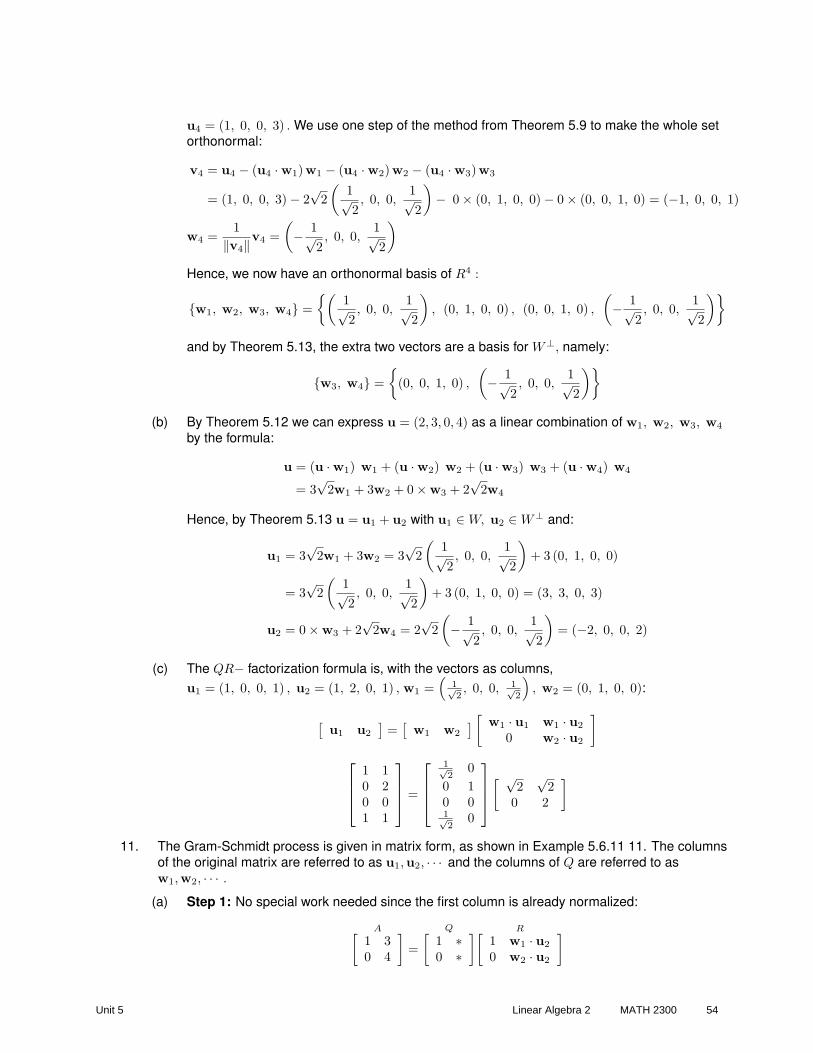
u4 = (1, 0, 0, 3) . We use one step of the method from Theorem 5.9 to make the whole setorthonormal:

v4 = u4 − (u4 ·w1)w1 − (u4 ·w2)w2 − (u4 ·w3)w3

= (1, 0, 0, 3)− 2√

2(

1√2, 0, 0,

1√2

)− 0× (0, 1, 0, 0)− 0× (0, 0, 1, 0) = (−1, 0, 0, 1)

w4 =1

‖v4‖v4 =(− 1√

2, 0, 0,

1√2

)

Hence, we now have an orthonormal basis of R4 :

{w1, w2, w3, w4} ={(

1√2, 0, 0,

1√2

), (0, 1, 0, 0) , (0, 0, 1, 0) ,

(− 1√

2, 0, 0,

1√2

)}

and by Theorem 5.13, the extra two vectors are a basis for W⊥, namely:

{w3, w4} ={

(0, 0, 1, 0) ,

(− 1√

2, 0, 0,

1√2

)}

(b) By Theorem 5.12 we can express u = (2, 3, 0, 4) as a linear combination of w1, w2, w3, w4

by the formula:

u = (u ·w1) w1 + (u ·w2) w2 + (u ·w3) w3 + (u ·w4) w4

= 3√

2w1 + 3w2 + 0×w3 + 2√

2w4

Hence, by Theorem 5.13 u = u1 + u2 with u1 ∈ W, u2 ∈ W⊥ and:

u1 = 3√

2w1 + 3w2 = 3√

2(

1√2, 0, 0,

1√2

)+ 3 (0, 1, 0, 0)

= 3√

2(

1√2, 0, 0,

1√2

)+ 3 (0, 1, 0, 0) = (3, 3, 0, 3)

u2 = 0×w3 + 2√

2w4 = 2√

2(− 1√

2, 0, 0,

1√2

)= (−2, 0, 0, 2)

(c) The QR− factorization formula is, with the vectors as columns,u1 = (1, 0, 0, 1) , u2 = (1, 2, 0, 1) , w1 =

(1√2, 0, 0, 1√

2

), w2 = (0, 1, 0, 0):

[u1 u2

]=

[w1 w2

] [w1 · u1 w1 · u2

0 w2 · u2

]

1 10 20 01 1

=

1√2

00 10 01√2

0

[ √2

√2

0 2

]

11. The Gram-Schmidt process is given in matrix form, as shown in Example 5.6.11 11. The columnsof the original matrix are referred to as u1,u2, · · · and the columns of Q are referred to asw1,w2, · · · .

(a) Step 1: No special work needed since the first column is already normalized:

A[1 30 4

]=

Q[1 ∗0 ∗

] R[1 w1 · u2

0 w2 · u2

]


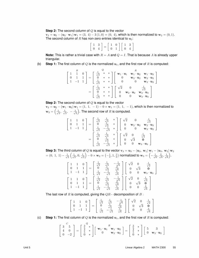
Step 2: The second column of Q is equal to the vectorv2 = u2 − (u2 ·w1)w1 = (3, 4)− 3 (1, 0) = (0, 4), which is then normalized to w2 = (0, 1).The second column of R has non-zero entries identical to u2:

[1 30 4

]=

[1 00 1

] [1 30 4

]

Note: This is rather a trivial case with R = A and Q = I. That is because A is already uppertriangular.

(b) Step 1: The first column of Q is the normalized u1, and the first row of R is computed:

B

1 1 00 1 11 −1 1

=

Q

1√2

∗ ∗0 ∗ ∗1√2

∗ ∗

R

w1 · u1 w1 · u2 w1 · u3

0 w2 · u2 w2 · u3

0 0 w3 · u3

=

1√2

∗ ∗0 ∗ ∗1√2

∗ ∗

√

2 0 1√2

0 w2 · u2 w2 · u3

0 0 w3 · u3

Step 2: The second column of Q is equal to the vectorv2 = u2 − (w1 · u2)w1 = (1, 1, − 1)− 0×w1 = (1, 1, − 1), which is then normalized tow2 =

(1√3, 1√

3, − 1√

3

). The second row of R is computed.

1 1 00 1 11 −1 1

=

1√2

1√3

∗0 1√

3∗

1√2

− 1√3

∗

√

2 0 1√2

0 w2 · u2 w2 · u3

0 0 w3 · u3

=

1√2

1√3

∗0 1√

3∗

1√2

− 1√3

∗

√

2 0 1√2

0√

3 00 0 w3 · u3

Step 3: The third column of Q is equal to the vector v3 = u3 − 〈u3, w1〉w1 − 〈u3, w2〉w2

= (0, 1, 1)− 1√2

(1√2, 0, 1√

2

)− 0×w2 =

(− 12 , 1, 1

2

)normalized to w3 =

(− 1√

6, 2√

6, 1√

6

).

1 1 00 1 11 −1 1

=

1√2

1√3

− 1√6

0 1√3

2√6

1√2

− 1√3

1√6

√

2 0 1√2

0√

3 00 0 w3 · u3

1 1 00 1 11 −1 1

=

1√2

1√3

− 1√6

0 1√3

2√6

1√2

− 1√3

1√6

√2 0 1√

2

0√

3 00 0 3√

6

The last row of R is computed, giving the QR− decomposition of B :

1 1 00 1 11 −1 1

=

1√2

1√3

− 1√6

0 1√3

2√6

1√2

− 1√3

1√6

√2 0 1√

2

0√

3 00 0 3√

6

(c) Step 1: The first column of Q is the normalized u1, and the first row of R is computed:

C

3 54 00 −2

=

Q

35 ∗45 ∗0 ∗

R[w1 · u1 w1 · u2

0 w2 · u2

]=

35 ∗45 ∗0 ∗

[5 30 w2 · u2

]


Step 2: The second column of Q is equal to the vectorv2 = u2 − (w1 · u2)w1 = (5, 0, − 2)− 3

(35 , 4

5 , 0)

=(

165 , − 12

5 , − 2)

which is then

normalized to w2 =(

85√

5, − 6

5√

5, − 1√

5

)The second row of R is computed giving the QR−

factorization:

3 54 00 −2

=

35

85√

545 − 6

5√

5

0 − 1√5

[5 30 w2 · u2

]=

Q

35

85√

545 − 6

5√

5

0 − 1√5

R[5 30 2

√5

]

(d) Step1: By Theorem 5.9, the matrices have the following form, with the first column of Qbeing the normalized u1. The first row of R is then computed:

D

1 0 20 1 32 −1 1

=

Q

1√5

∗ ∗0 ∗ ∗2√5

∗ ∗

R

w1 · u1 w1 · u2 w1 · u3

0 w2 · u2 w2 · u3

0 0 w3 · u3

=

1√5

∗ ∗0 ∗ ∗2√5

∗ ∗

√

5 − 2√5

4√5

0 w2 · u2 w2 · u3

0 0 w3 · u3

Step 2: The second column of Q is equal to the vectorv2 = u2 − (u2 ·w1)w1 = (0, 1, − 1)−

(− 2√

5

)(1√5, 0, 2√

5

)=

(25 , 1, − 1

5

), which is then

normalized to w2 =√

56

(25 , 1, − 1

5

)=

( √6

3√

5,√

5√6, − 1√

5√

6

). The second row of R is then

computed:

1 0 20 1 32 −1 1

=

1√5

√6

3√

5∗

0√

5√6

∗2√5

− 1√5√

6∗

√

5 − 2√5

4√5

0 w2 · u2 w2 · u3

0 0 w3 · u3

=

1√5

√6

3√

5∗

0√

5√6

∗2√5

− 1√5√

6∗

√5 − 2√

54√5

0√

65

3√

6√5

0 0 w3 · u3

Step 3: The third column of Q is equal to the vector:

v3 = u3 − (w1 · u3)w1 − (w2 · u3)w2

= (2, 3, 1)− 4√5

(1√5, 0,

2√5

)− 3

√6√5

( √6

3√

5,

√5√6,− 1√

5√

6

)

v3 = (0, 0, 0)

The zero vector found for v3 indicates that it is not possible to find a third non-zero vectororthogonal to the first two columns of Q. This happens because the original matrix D has alinear dependence in its columns (the third column equals 3 times the second plus 2 timesthe first), and so the columns of D only span a 2-dimensional subspace of R3.Note: Some authors produce a QR− factorization anyway, by finding an extra non-zerocolumn that makes Q orthogonal and then putting the bottom row of R to be all zeros, giving:

1 0 20 1 32 −1 1

=

1√5

√6

3√

5

√2√3

0√

5√6

− 1√6

2√5

− 1√5√

6− 1√

6

√5 − 2√

54√5

0√

65

3√

6√5

0 0 0


5.7 Least squares approximationsWhen S is a subspace of an inner product space V any vector b not in S is shown to have a uniqueorthogonal projection vector in the space S, denoted projS b, such that b− projS b is orthogonal toevery vector in S. The orthogonal projection vector solves an optimization problem because it is thenearest vector in S to the vector b, when distance is defined in terms of the inner product of V. In thisoptimization context, projS b is often referred to as the least squares approximation of the vector bwhen V is a Euclidean vector space.

We have previously encountered some orthogonal projection formulae. In Euclidean spaces in Unit 3Section 7: Linear Transformations from Rn to Rm, Theorem 3.14 gives the orthogonal projection onto aline through the origin, and Theorem 3.19 gives the orthogonal projection onto a plane through theorigin. We also encountered the general inner product space formula for the orthogonal projection ontoa line/vector through the origin in Theorem 5.7 of Unit 5 Section 5, Basic Properties of Inner ProductSpaces. Finally we saw a formula for the orthogonal projection onto a subspace of an inner productspace with a known orthogonal basis, in Theorem 5.13 of Unit 5, Section 6, Orthogonal Bases, theGram-Schmidt Process and QR− factorization. In this section we develop some formulae fororthogonal projections that work for any subspace of an inner product space and specificspecializations of these formulae for Euclidean spaces. The orthogonal projection, or least squaresapproximation, has a wide variety of applications in Engineering, Science, and Mathematics.

Note: Some of the proofs of theorems are omitted here but can be found in your textbook. Vectors areshown interchangeably as column matrices and as comma - separated row vectors. The word”projection” is often used here to mean ”orthogonal projection.”

5.7.1 Properties of orthogonal projections in inner product spacesDefinition.If S is a subspace of an inner product space V , and b /∈ S is any vector in V then the orthogonalprojection (or simply projection) of b in S is a vector y ∈ S such that b− y is orthogonal to everyvector in S. If b is in S we formally define the projection of b in S to be b (the same vector). Theprojection is denoted as projS b.

Note: Think of going from b along a line that is perpendicular to every vector in S until the line meets Sat the vector y =projS b. You can also think of it as being analogous to the Euclidean space projectionthat is easy to visualize, at least for R2 and R3. The picture for R2 is shown in Figure 5.5, and a similarpicture for R3 can be found in Unit 3, Linear Transformations from Rn to Rm.

Theorem 5.15. In any inner product space, the orthogonal projection projS b, of a vector b into a finitedimensional subspace S, always exists and is unique.

Proof. The subspace S must have a basis, and this basis can be converted to an orthogonal basisusing the Gram-Schmidt algorithm of the previous section, Orthogonal Bases, the Gram-SchmidtProcess, and QR− factorization. Furthermore Theorem 5.13 of the previous section gives a formula forthe orthogonal projection in terms of this orthogonal basis - hence, the projection always exists.

In order to show it is unique, suppose y1 and y2 are both projections of b. Since y1, y2 ∈ S :

〈b− y1, y1〉 = 0 =⇒ 〈b, y1〉 = 〈y1, y1〉〈b− y1, y2〉 = 0 =⇒ 〈b, y1〉 = 〈y1, y2〉

}and 〈b− y2, y2〉 = 0 =⇒ 〈b, y2〉 = 〈y2, y2〉

〈b− y2, y1〉 = 0 =⇒ 〈b, y2〉 = 〈y2, y1〉}

Since 〈y1, y2〉 = 〈y2, y1〉 (basis axiom that inner products are commutative) it follows that:

〈y1, y1〉 = 〈y2, y2〉 = 〈y1, y2〉 = 〈y2, y1〉


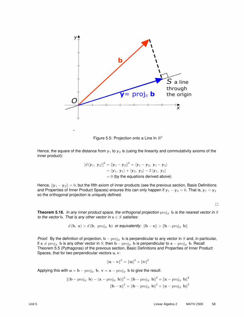
Figure 5.5: Projection onto a Line In R2

Hence, the square of the distance from y1 to y2 is (using the linearity and commutativity axioms of theinner product):

[d (y1, y2)]2 = ‖y1 − y2‖2 = 〈y1 − y2, y1 − y2〉

= 〈y1, y1〉+ 〈y2, y2〉 − 2 〈y1, y2〉= 0 (by the equations derived above)

Hence, ‖y1 − y2‖ = 0, but the fifth axiom of inner products (see the previous section, Basis Definitionsand Properties of Inner Product Spaces) ensures this can only happen if y1 − y2 = 0. That is, y1 = y2

so the orthogonal projection is uniquely defined.

Theorem 5.16. In any inner product space, the orthogonal projection projS b is the nearest vector in Sto the vector b. That is any other vector in x ∈ S satisfies:

d (b, x) > d (b, projS b) or equivalently: ‖b− x‖ > ‖b− projS b‖

Proof. By the definition of projection, b− projS b is perpendicular to any vector in S and, in particular,if x 6= projS b is any other vector in S, then b− projS b is perpendicular to x− projS b. RecallTheorem 5.5 (Pythagoras) of the previous section, Basic Definitions and Properties of Inner ProductSpaces, that for two perpendicular vectors u,v:

‖u− v‖2 = ‖u‖2 + ‖v‖2

Applying this with u = b− projS b, v = x− projS b to give the result:

‖(b− projS b)− (x− projS b)‖2 = ‖b− projS b‖2 + ‖x− projS b‖2

‖b− x‖2 = ‖b− projS b‖2 + ‖x− projS b‖2


However, ‖x− projS b‖2 > 0, since x− projS b 6= 0, and so:

‖b− x‖2 > ‖b− projS b‖2 =⇒ ‖b− x‖ > ‖b− projS b‖ , as asserted.

Theorem 5.17. Suppose V is an inner product space, and S is a 2-dimensional subspace with a basis{v1, v2}. If the orthogonal projection vector is given by the linear combination of these basis vectors as:

projS b = k1v1 + k2v2 where k1, k2 ∈ R

then k1, k2 are solutions of the linear equations with non-singular coefficient matrix:[ 〈v1, v1〉〈v1, v2〉〈v2, v1〉〈v2, v2〉

] [k1

k2

]=

[ 〈v1, b〉〈v2, b〉

]

Note: The matrix is symmetric because 〈v2, v1〉 = 〈v1, v2〉 .

Proof. If b− projS b is orthogonal to v1 and v2 then it is left as an exercise for the reader to show thatb− projS b is orthogonal to all vectors in S. Hence, we have the two equations (using projS b− binstead of b− projS b):

〈projS b− b, v1〉 = 0〈projS b− b, v2〉 = 0

}=⇒ 〈k1v1 − k2v2 − b, v1〉 = 0

〈k1v1 − k2v2 − b, v2〉 = 0

}=⇒ k1 〈v1, v1〉+ k2 〈v2, v1〉 = 〈b, v1〉

k1 〈v1, v2〉+ k2 〈v2, v2〉 = 〈b, v2〉}

The matrix form of the two equations is the required result (using the commutativity 〈b, v1〉 = 〈v1, b〉,〈b, v2〉 = 〈v2, b〉 , 〈v2, v1〉 = 〈v1, v2〉.

The determinant of the coefficient matrix is (where θ is the angle between the two basis vectors):

〈v1, v1〉〈v2, v2〉 − 〈v1, v2〉2 = ‖v1‖2 ‖v2‖2 − ‖v1‖2 ‖v2‖2 cos2 θ

= ‖v1‖2 ‖v2‖2(1− cos2 θ

)

= ‖v1‖2 ‖v2‖2 sin2 θ

This is zero only if one of ‖v1‖ , ‖v2‖ is zero, in which case that vector is the zero vector, and so not abasis vector, or, sin θ = 0 in which case θ = 0 and v1, v2 are parallel vectors and so cannot be a basisof S. Hence, the determinant cannot be zero when {v1, v2} is a basis, and so the coefficient matrix isnon-singular.

Theorem 5.18. Suppose V is an inner product space, and S is a k− dimensional subspace with abasis {v1, v2, · · · , vk}. If the orthogonal projection vector is given by the linear combination of thesebasis vectors as:

projS b = k1v1 + k2v2 + · · ·+ kkvk where k1, k2, · · · , kk ∈ R

then k1, k2 2, · · · , kk are solutions of the k × k system of linear equations with k × k non-singularcoefficient matrix:

〈v1, v1〉〈v1, v2〉 · · · 〈v1, vk〉〈v2, v1〉〈v2, v2〉 · · · 〈v2, vk〉

......

. . ....

〈vk, v1〉〈vk, v2〉 · · · 〈vk, vk〉

k1

k2

...kk

=

〈v1, b〉〈v2, b〉

...〈vk, b〉

Note: The matrix is symmetric because⟨vi, vj

⟩= 〈vj , vi〉 for each i, j.


Proof. The proof is not given but is similar to the proof of Theorem 5.17.

Example 5.7.1.In P3 find the projection of the polynomial f (x) = 2− 3x + 4x2 onto the subspace S with basis{b1 (x) , b2 (x)} =

{x, x2

}

(a) Using the inner product⟨a0 + a1x + a2x

2, b0 + b1x + b2x2⟩

= a0b0 + a1b1 + a2b2

(b) Requires calculus. Using the inner product 〈f, g〉 =∫ 1

−1f (x) g (x) dx


(a) If the projection is the linear combination of the basis vectors p (x) = k1x + k2x2 then by Theorem

5.17, k1, k2 satisfies:[ 〈b1, b1〉〈b1, b2〉〈b2, b1〉〈b2, b2〉

] [k1

k2

]=

[ 〈b1, f〉〈b2, f〉

]

[1 00 1

] [k1

k2

]=

[ −34

]

with solution k1 = −3, k2 = 4. Hence, the projection of f (x) = 2− 3x + 4x2 onto the subspacewith basis

{x, x2

}is the polynomial:

p (x) = −3x + 4x2

Note: The projection just drops the constant term of the polynomial, which seems intuitivelyreasonable.

(b) If the projection is the linear combination of the basis vectors p (x) = k1x + k2x2 then by Theorem

5.17, k1, k2 satisfies:[ 〈b1, b1〉〈b1, b2〉〈b2, b1〉〈b2, b2〉

] [k1

k2

]=

[ 〈b1, f〉〈b2, f〉

]

[ ∫ 1

−1x2 dx

∫ 1

−1x3 dx∫ 1

−1x3 dx

∫ 1

−1x4 dx

] [k1

k2

]=

[ ∫ 1

−1x

(2− 3x + 4x2

)dx∫ 1

−1x2

(2− 3x + 4x2

)dx

]

Evaluating the integrals (details not shown) the equations become:[

23 00 2

5

] [k1

k2

]=

[ −24415

]

with solution k1 = −3, k2 = 223 . Hence, the projection of f (x) = 2− 3x + 4x2 onto the subspace

with basis{x, x2

}is the polynomial:

p (x) = −3x +223

x2

Note: To check the accuracy of the result in part (b), compute the f (x)− p (x) = 2− 103 x2 (that is

f (x)− projS f ), and show it is orthogonal to the basis polynomials, b1 (x) and b2 (x). That is,check that: ∫ 1

−1

x

(2− 10

3x2

)dx = 0 and

∫ 1

−1

x2

(2− 10

3x2

)dx = 0


Example 5.7.2.Find the orthogonal projection of the matrix A onto the subspace S of M22 with basis {B, C} , usingthe usual inner product (scalar product of the vectors formed from the four coefficients of the matrices):

A =[

2 0−3 2

], B =

[1 00 1

], C =

[0 11 1

]

Solution. If the projection is the linear combination of the basis vectors D = k1B + k2C then byTheorem 5.17, k1, k2 satisfies:

[ 〈B, B〉〈B, C〉〈C, B〉〈C, C〉

] [k1

k2

]=

[ 〈B, A〉〈C, A〉

]

[2 11 3

] [k1

k2

]=

[4−1

]

with solution k1 = 135 , k2 = − 6

5 . Hence, the projection is:

D =135

[1 00 1

]− 6

5

[0 11 1

]=

[135 − 6

5− 6

575

]

Note: To check the accuracy of the result in part (b), compute A−D =[ − 3

565

− 95

35

](that is

A− projS A), and show it is orthogonal to the basis matrices B,C. That is, check that:

〈A−D, B〉 = 0 and 〈A−D,C〉 = 0

5.7.2 Properties of orthogonal projections in Euclidean spaces Rn

Euclidean spaces, Rn, n = 1, 2, 3, · · · are inner product spaces. We assume the usual inner product〈u, v〉 = u · v - the scalar product. The orthogonal projection in a Euclidean space Rn is often calledthe Least Squares Approximation. The reason for this name is that if b is a vector and y = projS b isits projection on a subspace S then y is the nearest vector to b in S. Hence, if e = b− y is the ”error”vector of the approximation of b by y then the length ‖e‖ is minimized. However:

‖e‖ =√

e21 + e2

2 + · · ·+ e2n

where e1, e2, · · · , en are the components of e, and so the orthogonal projection minimizes the sum ofthe squares of the ei - that is it finds the least value of the sum of squares.

The results in the previous section for general Inner Product Spaces, hold in Euclidean spaces but havesome extra features. Theorem 5.17 becomes:

Theorem 5.19. Suppose that in Rn, for some n > 2, S is a 2-dimensional subspace with a basis{v1, v2}. If the orthogonal projection of the vector b is given by the linear combination of these basisvectors as:

projS b = k1v1 + k2v2 where k1, k2 ∈ R

then k1, k2 are solutions of the linear equations with symmetric non-singular coefficient matrix:[

v1 · v1 v1 · v2

v2 · v1 v2 · v2

] [k1

k2

]=

[v1 · bv2 · b

]

This can also be re-written in terms of products of matrices as:

AT AX = AT B


where:AT[vT

1−−−vT

2

]A[

v1| v2

] X[k1

k2

]=

AT[vT

1−−−vT

2

]B

[b]

That is, the matrix A has the column vectors v1, v2 as columns, the transpose matrix AT has thevectors v1, v2 as rows, and B has the single vector b as its column.

Note: The matrix equations AT AX = AT B are called the normal equations and are usually deriveddirectly using matrix/vector methods in Rn without appealing to the general theorem of inner productspaces.

Proof. The first matrix equation containing the scalar products follows directly from Theorem 5.17. Theproof that this is the same as the second matrix form follows directly by using block matrix multiplicationof the rows vT

1 ,vT2 of AT by the columns v1,v2,b of A and B:

[vT

1−−−vT

2

][

v1| v2

] [k1

k2

]=

[vT

1−−−vT

2

][b] =⇒

[vT

1 v1 vT1 v2

vT2 v1 vT

2 v2

] [k1

k2

]=

[vT

1 bvT

2 b

]

Since vTi vj = vi · vj and vT

i b = vi · b this last equation is the same as first matrix equation of thetheorem.

Theorem 5.20. Suppose that in Rn, for some n > k, S is a k− dimensional subspace with a basis{v1, v2, · · · ,vk}. If the orthogonal projection of the vector b is given by the linear combination of thesebasis vectors as:

projS b = k1v1 + k2v2 + · · ·+ kkvk where k1, k2, · · · , kk ∈ R

then k1, k2, · · · , kk are solutions of the linear equations with symmetric non-singular coefficient matrix:

v1 · v1 v1 · v2 · · · v1 · vk

v2 · v1 v2 · v2 · · · v2 · vk

......

. . ....

vk · v1 vk · v2 · · · vk · vk

k1

k2

...kk

=

v1 · bv2 · b

...vk · b

This can also be re-written in terms of products of matrices as:

AT AX = AT B

where:AT

vT1

vT2...

vTk

A[v1 v2 · · · vk

]

X

k1

k2

...kk

=

AT

vT1

vT2...

vTk

B

[b]

That is, the matrix A has the column vectors v1, v2, · · · ,vk as columns, the transpose matrix AT hasthe row vectors vT

1 , vT2 , · · · ,vT

k as rows, and B has the single vector b as its column.

Proof. The proof is not given here, but it would use methods analogous to the proof of Theorem5.19.


Theorem 5.21. Suppose that in Rn, for some n > k, S is a k− dimensional subspace with a basis{v1, v2, · · · ,vk}, and A has the vi as columns:

A =[

v1 v2 · · · vk

]

The projection matrix P, such that for any b ∈ Rn, Pb is the projection of b onto S is given by:

P = A(AT A

)−1AT

Proof. From Theorem 5.20, the matrix AT A is non-singular, and the projection satisfies:

projS b = k1v1 + k2v2 + · · ·+ kkvk =A[

v1 v2 · · · vk

]

X

k1

k2

...kk

= AX

X is the solution of AT AX = AT B, where B = [b]. This is given by the inverse matrix method as:

X =(AT A

)−1AT B

and so the projection is:P = AX = A

(AT A

)−1AT B

and so the projection matrix is A(AT A

)−1AT .

Example 5.7.3.Find the orthogonal projection of the vector b = (1, 2, 3) onto the subspace S with basis{v1, v2} = {(1, 0, 2) , (0,−1, 3)} .

Solution. If the projection is p = k1v1 + k2v2 then, using Theorem 5.19, the equations satisfied byk1, k2 are: [

v1 · v1 v1 · v2

v2 · v1 v2 · v2

] [k1

k2

]=

[v1 · bv2 · b

]=⇒

[5 66 10

] [k1

k2

]=

[77

]

with solution k1 = 2, k2 = − 12 . Hence, the orthogonal projection is:

p = 2 (1, 0, 2)− 12

(0,−1, 3) =(

2,12,52

)

Note: To check the accuracy of this result, show that b− p =(−1, 3

2 , 12

)is orthogonal to the basis

vectors v1, v2. That is, check that:(−1,

32,12

)· (1, 0, 2) = 0 and

(−1,

32,12

)· (0,−1, 3) = 0

Note: The alternative way of setting-up the equations, used in most textbooks, is as follows. Constructthe matrices, A with the basis vectors as columns and B with b as its column:

A =

1 00 −12 3

, B =

123


Compute the normal equations AT AX = AT B (these will be the same as the equations used above tosolve this example):

AT[1 0 20 −1 3

] A

1 00 −12 3

[k1

k2

]=

AT[1 0 20 −1 3

] B

123

After multiplying the first two matrices on each side these become:[

5 66 10

] [k1

k2

]=

[77

]

5.7.3 Applications of least squares in Euclidean spaces Rn

Approximate solutions of inconsistent systems of equationsIn many applications the solution of a problem is given by the solution of a linear system of equations,but this system turns out to be inconsistent (it does not have a solution). This can happen when there isan excess of data that produces more equations than unknowns and inaccuracies in the data or modelused ensure this system is inconsistent. In other applications the model deliberately creates aninconsistent system and requires a best possible approximate solution to the system (see Example5.7.5 below).

There are many ways to find an approximate solution to an inconsistent system. The Least SquaresApproximation of an inconsistent system AX = B uses results established in Theorems 5.19, 5.20and 5.21 that are, for convenience, re-written in equation terminology in Theorem 5.22.

Theorem 5.22. Suppose a linear system is AX = B, whereA is an m× n matrix with m ≥ n, X is then× 1 column of unknowns, and B is the m× 1 column vector of right hand values. The least squaresapproximate solution for X of the system is defined to be the orthogonal projection of B onto the spacespanned by the columns of A, and it is given by the solution of the normal equations:

AT AX = AT B

The least squares approximation minimizes the sum of the squares of the differences between the righthand side and left hand side of each of the equations (that is, each row of AX = B). If the columns ofA are linearly independent then the coefficient matrix AT A is non-singular and then the solution can bewritten:

X =(AT A

)−1AT B

The orthogonal projection of B onto the column space of A is given by:

AX = A(AT A

)−1AT B, and the projection matrix is: A

(AT A

)−1AT

Note: This formula holds even if the original system is consistent (has an exact solution). In that casethe least squares approximation is the same as the exact solution of the system. When the columns ofA are linearly dependent, the coefficient matrix AT A is singular, and the normal equations haveinfinitely many solutions, but all of these will give the same value of AX.

Proof. This theorem is a variation of Theorems 5.19 and 5.20. To make the connection clearer, notethat AX is simply a linear combination of the column vectors of A. That is if, in column form,A =

[v1| v2| · · · | vn

]and XT =

[x1 x2 · · · xn

]then:

AX =[

v1| v2| · · · | vn

]

x1

x2

...xn

= x1v1 + x2v2 + · · ·+ xnvn


Hence, the problem is to find the orthogonal projection of the right hand side B onto the subspacespanned by columns of A - the problem solved by Theorems 5.19 and 5.20.

Theorems 5.19 and 5.20 did not cover the case where the matrix AT A is singular (because thecolumns of A are linearly dependent). However, in that case, if X is any one solution of the normalequations AT AX = AT B the all other solutions are given by X + Y where Y is any vector in the nullspace of A. In that case all solutions give the same value of for the projection AX becauseA (X + Y ) = AX + AY = AX.

Example 5.7.4.Find the least squares approximation, and find the error in the solution for the system of equationsAX = B:

1 −3−2 41 −4

[x1

x2

]=

216

Solution. Solving the first two equations gives x1 = − 112 , x2 = − 5

2 , but these two values do not satisfythe third equation, so the system is inconsistent. Using the method of Theorem 5.19, the least squareapproximation X is the solution of the normal equations AT AX = AT B, and this is:

[1 −2 1−3 4 −4

]

1 −3−2 41 −4

[x1

x2

]=

[1 −2 1−3 4 −4

]

216

[6 −15−15 41

] [x1

x2

]=

[6−26

]

with solution x1 = − 487 and x2 = − 22

7 . The differences between the left and right sides gives the errorvector:

1 −3−2 41 −4

[ − 487

− 227

]−

216

=

18787407

−

216

=

4717− 2

7

Hence, the errors in the three equations are 47 , 1

7 ,− 27 .

Note: The method actually minimizes the sum of the squares of the errors. That is, in this example,(47

)2 +(

17

)2 +(− 2

7

)2 = 37 is as small as it possibly can be.

Note: In many inconsistent systems of equations it would be better to minimize the sums of theabsolute values of the errors (rather than the squares of these), but this is a more difficult problem tosolve. In particular, when an inconsistent system has an equation constructed from data that is totallywrong, then the least squares method tends to exaggerate the affect of that invalid equation on theapproximate solution (rather than minimizing it).

Linear regressionExample 5.7.5.A large set of data in R2: (xi, yi) , i = 1, 2, · · · ,m is obtained in an experiment. The data should lie on astraight line but experimental errors, or inaccuracies in the model, have ensured that the data does notlie on a straight line. The experimenters want to find a straight line, y = a + bx, that best fits the data,and they decide to minimize the sums of the squares of the deviations in the y− values. Show that thevalues for a, b are given by:

a =

∑y∑

x2 −∑

x∑

xy

m∑

x2 −(∑

x)2 , b =

m∑

xy −∑

x∑

y

m∑

x2 −(∑

x)2


where the formulae use the following abbreviations for clarity:∑

xy meansm∑

i=1

xiyi,∑

x meansm∑

i=1

xi,

∑y means

m∑

i=1

yi,∑

x2meansm∑

i=1

x2i .

Solution. Set up each data point for the equation in the form a + bx = y, with unknowns a and b :

a + bx1 = y1

a + bx2 = y2

a + bx3 = y3

...a + bxm = ym

=⇒

1 x1

1 x2

1 x3

......

1 xm

[ab

]=

y1

y2

y3

...ym

This is (almost certainly) an inconsistent system of the form AX = B, and so we can solve it by themethod of Theorem 5.22, by solving the system AT AX = AT B :

1 1 1

... 1

x1 x2 x3

... xm

1 x1

1 x2

1 x3

......

1 xm

[ab

]=

1 1 1

... 1

x1 x2 x3

... xm

y1

y2

y3

...ym

m∑

i=1

1∑

x

∑x

∑x2

[ab

]=

[ ∑y∑xy

]

Noting thatm∑

i=1

1 = m, the solution given by the formula for the inverse of a 2× 2 matrix is:

[ab

]=

1

m∑

x2 −(∑

x)2

[ ∑x2 −

∑x

−∑

x m

][ ∑y∑xy

]

[ab

]=

1

m∑

x2 −(∑

x)2

[ ∑y∑

x2 −∑

x∑

xy

m∑

xy −∑

x∑

y

]=

∑y

∑x2−

∑x

∑xy

m

∑x2−

�∑x

�2

m

∑xy−

∑x

∑y

m

∑x2−

�∑x

�2

Note: The regression line is a basic result in statistics ,where it is often written in a simpler form using

statistical constructs: x =∑

x

m (the mean of the xi values), y =∑

y

m . The formulae become (see theexercise set for more details):

b =∑

(x− x) (y − y)∑(x− x)2

and a = y − bx

Note: See the exercise set for numerical examples using this formula.

Least squares approximations for nonlinear functionsThe least squares method uses linear methods but it can be used to find least squares data fits, usingpolynomials and exponential functions.


Example 5.7.6.A given set of data in R2: (xi, yi) , i = 1, 2, · · · ,m is expected to fit a quadratic function but experimentalerrors, or inaccuracies in the model, have ensured that no quadratic fits it exactly. We want to find aquadratic, y = a + bx + cx2, by minimizing the sums of the squares of the deviations in the y− values.Show that the values of a, b, c are given by the solutions of the normal equations AT AX = AT B, where:

A =

1 x1 x21

1 x2 x22

1 x3 x23

......

...1 xm x2

m

, X =

abc

, B =

y1

y2

y3

...ym

Solution. Set up each data point for the equation in the form a + bx + cx2 = y, with unknowns a, b, c :

a + bx1 + cx21 = y1

a + bx2 + cx22 = y2

a + bx3 + cx23 = y3

...a + bxm + cx2

m = ym

=⇒

1 x1 x21

1 x2 x22

1 x3 x23

......

...1 xm x2

m

abc

=

y1

y2

y3

...ym

This is (almost certainly) an inconsistent system of the form AX = B and so we can solve it by themethod of Theorem 5.22 (and Example 5.7.5) by solving the system AT AX = AT B as asserted.

Note: For numerical examples, see the exercise set.

Note: A method exactly analogous to this example can be used to find polynomials of any degree thatapproximate a data set. However, the problem becomes numerically unstable if the degree of thepolynomial is large. The process generally works reasonably well with polynomials of degree 3 and 4.

Note: The method will also become unstable and may give meaningless results if the data really doesnot all lie reasonably close to a polynomial of the degree used in the approximation.

Example 5.7.7.A given set of data in R2: (xi, yi) , i = 1, 2, · · · ,m is expected to fit an exponential function, y = aebx,but experimental errors, or inaccuracies in the model, have ensured that no such function fits it exactly.We want to find an exponential function y = aebx by minimizing the sums of the squares of thedeviations in the y− values. Show that the values of a, b are given by the solutions of the normalequations AT AX = AT B, where:

A =

1 x1

1 x2

1 x3

......

1 xm

, X =[

ln ab

], B =

ln y1

ln y2

ln y3

...ln ym

Solution. Set up each data point for the equation in the form aebx = y, with unknowns a, b :

aebx1 = y1

aebx2 = y2

aebx3 = y3

...aebxm = ym

Take logs of=⇒

both sides

ln a + bx1 = ln y1

ln a + bx2 = ln y2

ln a + bx3 = ln y3

...ln a + bxm = ln ym

=⇒

1 x1

1 x2

1 x3

......

1 xm

[ln ab

]=

ln y1

ln y2

ln y3

...ln ym


This is (almost certainly) an inconsistent system of the form AX = B, and so we can solve it by themethod of Theorem 5.22 (and Examples 5.7.5, 5.7.6) by solving the system AT AX = AT B asasserted.

Note: For numerical examples, see the exercise set.

Note: The solution does not actually solve the problem as stated, because it actually finds the leastsquares solution of the equations formed by taking logs of both sides. That is, the solution is not a leastsquares solution of the original equations aebxi = yi.


1. Find the orthogonal projection in R3 of the vector (1, 2, 3) onto the two-dimensional subspacespanned by the vectors {(2, 0,−3) , (2, 1, 1)}, using the inner product:

(a) The normal scalar product

(a) The inner product: 〈(a, b, c) , (e, f, g)〉 = ae + bf + 2cg

2. Find the orthogonal projection in P4 of the polynomial f (x) = x + x4 onto P2 with basis{b1 (x) , b2 (x) , b3 (x)} =

{1, x, x2

}using the inner product:

(a)⟨a0 + a1x + a2x

2 + a3x3 + a4x

4, b0 + b1x + b2x2 + b3x

3 + b4x4⟩

= a0b0 + a1b1 + a2b2 + a3b3 + a4b4

(b) Requires calculus: 〈p, q〉 =∫ 1

−1p (x) q (x) dx

3. Find the projection of the matrix A onto the subspace of M22 spanned by the matrices B, C, Dwith the inner product defined in the usual way as the scalar product of the vectors formed fromthe four entries in each matrix or, equivalently, as the trace (sum of diagonal values) of thetranspose of one matrix multiplied by the other matrix.

A =[

2 10 2

], B =

[1 01 1

], C =

[0 11 1

], D =

[1 11 0

]

4. Find the projection matrix P for the projection in R4 onto the subspace S spanned by the twovectors:

{(1, 3,−2, 1) , (0, 1, 0, 1)}That is, Pv gives the orthogonal projection of v in S.

5. Find the least squares approximation, and find the errors in each equation, for the linear systemsAX = B:

(a) when:

A =

2 0−1 20 1

, B =

2−13

(b) when:

A =

2 0−1 20 1

, B =

211

and explain the meaning of the unusual set of errors.


(c) when:

A =

2 0 1−1 2 00 1 00 0 1

, B =

2−132

6. Find the regression line for the data:

{(0, 1) , (1, 1.3) , (2, 1.9) , (3, 2.6) , (4, 3)}

7. More difficult and needs a calculator or computer. Find a plane that fits the data:

(xi, yi, zi) = {(0, 1, 1) , (1, 1.3, 1.9) , (2, 1.9, 3.1) , (3, 2.6, 4.2) , (4, 3, 4.8)}That is, assume the plane is z = a + bx + cy, and do the least squares fit on the z− values.

8. More difficult. Given the data:

{(0, 2) , (1, 0) , (2, − 1) , (3, 0) , (4, 1)}(a) Find a quadratic, y = a + bx + cx2, that gives the best least squares fit to the data. Find the

sum of squares of the errors.(b) Find a cubic, y = a + bx + cx2 + dx3, that gives the best least squares fit to the data. Find the

sum of squares of the errors.

9. More difficult. Given the data:

{(−1, 0.5) , (0, 1) , (0.5, 2) , (1, 3) , (1.5, 5)}(a) Find an exponential, y = aebx, that gives the best least squares fit to the data. Find all of the

errors in the y− values.(b) Find a quadratic, y = a + bx + cx3, that gives the best least squares fit to the data. Find the

errors in the y− values.

10. Requires calculus and difficult. Find the orthogonal projection of f (x) = ex onto the set ofpolynomials {g1 (x) , g2 (x) , g3 (x) , g4 (x)} =

{1, x, x2, x3

}in the (infinite dimensional) vector

space of all continuous functions, with the inner product:

〈p, q〉 =∫ 1

−1

f (x) g (x) dx

11. More difficult. Show that the simpler forms of the formulae given in Example 5.7.5 are correct:

b =m

∑xy −

∑x∑

y

m∑

x2 −(∑

x)2 =

∑(x− x) (y − y)∑

(x− x)2

a =

∑y∑

x2 −∑

x∑

xy

m∑

x2 −(∑

x)2 = y − bx

Solutions

1. For the vector b = (1, 2, 3) , and subspace S spanned by {v1, v2} = {(2, 0,−3) , (2, 1, 1)} , theorthogonal projection of b onto S is given by p = k1v1 + k2v2, given by the solution of (Theorem5.17 ): [ 〈v1, v1〉〈v1, v2〉

〈v2, v1〉〈v2, v2〉] [

k1

k2

]=

[ 〈v1, b〉〈v2, b〉

]

and this becomes:


(a) For the normal scalar product:[

v1 · v1 v1 · v2

v2 · v1 v2 · v2

] [k1

k2

]=

[v1 · bv2 · b

]

[13 11 6

] [k1

k2

]=

[ −77

]

with solution k1 = − 711 , k2 = 14

11 . Hence, the orthogonal projection is:

p =(− 7

11

)(2, 0,−3) +

1411

(2, 1, 1) =(

1411

,1411

,3511

)

(b) For the inner product 〈(a, b, c) , (e, f, g)〉 = ae + bf + 2cg this becomes:[

22 −2−2 7

] [k1

k2

]=

[ −1610

]

with solution k1 = − 4675 , k2 = 94

75 . Hence, the orthogonal projection is:

p =(−46

75

)(2, 0,−3) +

9475

(2, 1, 1) =(

3225

,9475

,23275

)

2. Given f (x) = x + x4 and basis {b1 (x) , b2 (x) , b3 (x)} ={1, x, x2

}of P2, the projection of f onto

P2 is given by = p (x) = k1b1 (x) + k2b2 (x) + k3b3 (x) where k1, k2, k3 are given by:

(a) With inner product⟨a0 + a1x + a2x

2 + a3x3 + a4x

4, b0 + b1x + b2x2 + b3x

3 + b4x4⟩

= a0b0 + a1b1 + a2b2 + a3b3 + a4b4, solve:〈b1, b1〉〈b1, b2〉〈b1, b3〉〈b2, b1〉〈b2, b2〉〈b2, b3〉〈b3, b1〉〈b3, b2〉〈b3, b3〉

k1

k2

k3

=

〈b1, f〉〈b2, f〉〈b3, f〉

1 0 00 1 00 0 1

k1

k2

k3

=

010

=⇒

k1

k2

k3

=

010

Hence, the projection of f (x) = x + x4 is p (x) = x.

(b) With inner product 〈p, q〉 =∫ 1

−1p (x) q (x) dx, solve:

∫ 1

−11 dx

∫ 1

−1x dx

∫ 1

−1x2 dx∫ 1

−1x dx

∫ 1

−1x2 dx

∫ 1

−1x3 dx∫ 1

−1x2 dx

∫ 1

−1x3 dx

∫ 1

−1x4 dx

k1

k2

k3

=

∫ 1

−1

(x + x4

)dx∫ 1

−1x

(x + x4

)dx∫ 1

−1x2

(x + x4

)dx

2 0 23

0 23 0

23 0 2

5

k1

k2

k3

=

252327

=⇒

k1

k2

k3

=

− 3

35167

Hence, the projection of f (x) = x + x4 is p (x) = − 335 + x + 6

7x2.Note: To check your result, show that 〈f − p, bi〉 = 0 for each basis function bi. Sincef (x)− p (x) = 3

35 − 67x2 + x4, we have to show (the correct results):

∫ 1

−1

(335− 6

7x2 + x4

)dx = 0,

∫ 1

−1

(335

x− 67x3 + x5

)dx = 0

∫ 1

−1

(335

x2 − 67x4 + x6

)dx = 0


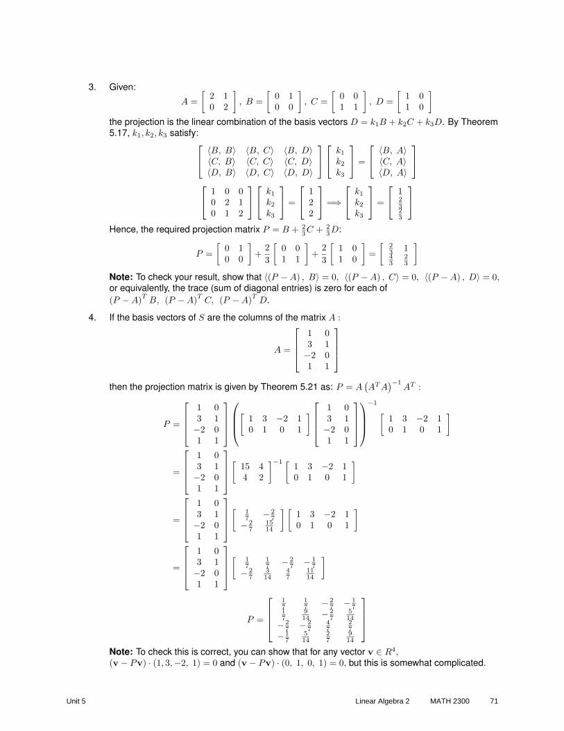
3. Given:

A =[

2 10 2

], B =

[0 10 0

], C =

[0 01 1

], D =

[1 01 0

]

the projection is the linear combination of the basis vectors D = k1B + k2C + k3D. By Theorem5.17, k1, k2, k3 satisfy:

〈B, B〉〈B, C〉〈B, D〉〈C, B〉〈C, C〉〈C, D〉〈D, B〉〈D, C〉〈D, D〉

k1

k2

k3

=

〈B, A〉〈C, A〉〈D, A〉

1 0 00 2 10 1 2

k1

k2

k3

=

122

=⇒

k1

k2

k3

=

12323

Hence, the required projection matrix P = B + 23C + 2

3D:

P =[

0 10 0

]+

23

[0 01 1

]+

23

[1 01 0

]=

[23 143

23

]

Note: To check your result, show that 〈(P −A) , B〉 = 0, 〈(P −A) , C〉 = 0, 〈(P −A) , D〉 = 0,or equivalently, the trace (sum of diagonal entries) is zero for each of(P −A)T

B, (P −A)TC, (P −A)T

D.

4. If the basis vectors of S are the columns of the matrix A :

A =

1 03 1−2 01 1

then the projection matrix is given by Theorem 5.21 as: P = A(AT A

)−1AT :

P =

1 03 1−2 01 1

[1 3 −2 10 1 0 1

]

1 03 1−2 01 1

−1

[1 3 −2 10 1 0 1

]

=

1 03 1−2 01 1

[15 44 2

]−1 [1 3 −2 10 1 0 1

]

=

1 03 1−2 01 1

[17 − 2

7− 2

71514

] [1 3 −2 10 1 0 1

]

=

1 03 1−2 01 1

[17

17 − 2

7 − 17

− 27

314

47

1114

]

P =

17

17 − 2

7 − 17

17

914 − 2

7514

− 27 − 2

747

27

− 17

514

27

914

Note: To check this is correct, you can show that for any vector v ∈ R4,(v − Pv) · (1, 3,−2, 1) = 0 and (v − Pv) · (0, 1, 0, 1) = 0, but this is somewhat complicated.


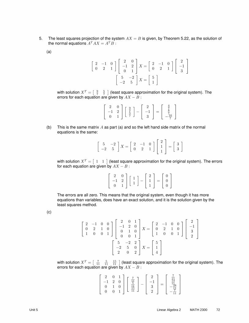
5. The least squares projection of the system AX = B is given, by Theorem 5.22, as the solution ofthe normal equations AT AX = AT B :

(a)

[2 −1 00 2 1

]

2 0−1 20 1

X =

[2 −1 00 2 1

]

2−13

[5 −2−2 5

]X =

[51

]

with solution XT =[

97

57

](least square approximation for the original system). The

errors for each equation are given by AX −B :

2 0−1 20 1

[9757

]−

2−13

=

4787

− 167

(b) This is the same matrix A as part (a) and so the left hand side matrix of the normalequations is the same:

[5 −2−2 5

]X =

[2 −1 00 2 1

]

211

=

[33

]

with solution XT =[

1 1]

(least square approximation for the original system). The errorsfor each equation are given by AX −B :

2 0−1 20 1

[11

]−

211

=

000

The errors are all zero. This means that the original system, even though it has moreequations than variables, does have an exact solution, and it is the solution given by theleast squares method.

(c)

2 −1 0 00 2 1 01 0 0 1

2 0 1−1 2 00 1 00 0 1

X =

2 −1 0 00 2 1 01 0 0 1

2−132

5 −2 2−2 5 02 0 2

X =

514

with solution XT =[

711

511

1511

](least square approximation for the original system). The

errors for each equation are given by AX −B :

2 0 1−1 2 00 1 00 0 1

7115111511

−

2−132

=

7111411− 28

11− 7

11


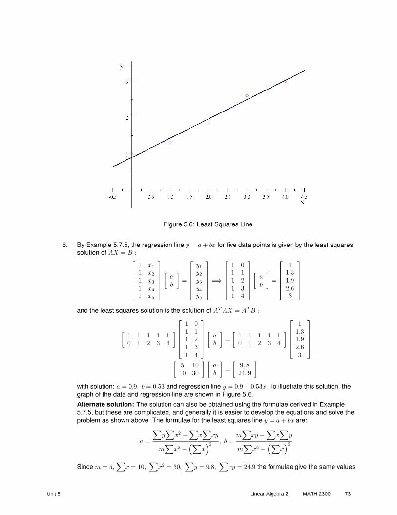
Figure 5.6: Least Squares Line

6. By Example 5.7.5, the regression line y = a + bx for five data points is given by the least squaressolution of AX = B :

1 x1

1 x2

1 x3

1 x4

1 x5

[ab

]=

y1

y2

y3

y4

y5

=⇒

1 01 11 21 31 4

[ab

]=

11.31.92.63

and the least squares solution is the solution of AT AX = AT B :

[1 1 1 1 10 1 2 3 4

]

1 01 11 21 31 4

[ab

]=

[1 1 1 1 10 1 2 3 4

]

11.31.92.63

[5 1010 30

] [ab

]=

[9. 824. 9

]

with solution: a = 0.9, b = 0.53 and regression line y = 0.9 + 0.53x. To illustrate this solution, thegraph of the data and regression line are shown in Figure 5.6.

Alternate solution: The solution can also be obtained using the formulae derived in Example5.7.5, but these are complicated, and generally it is easier to develop the equations and solve theproblem as shown above. The formulae for the least squares line y = a + bx are:

a =

∑y∑

x2 −∑

x∑

xy

m∑

x2 −(∑

x)2 , b =

m∑

xy −∑

x∑

y

m∑

x2 −(∑

x)2

Since m = 5,∑

x = 10,∑

x2 = 30,∑

y = 9.8,∑

xy = 24.9 the formulae give the same values


for a, b:

a =9.8× 30− 10× 24.9

5× 30− (10)2= 0.9

b =5× 24.9− 10× 9.8

5× 30− (10)2= 0.53

7. Extending the method of Example 5.7.5, the regression equation z = a + bx + cy: for five datapoints is given by the least squares solution of equations AX = B formed by inserting the data inthe form a + bx + cy = z

1 x1 y1

1 x2 y2

1 x3 y3

1 x4 y4

1 x5 y5

abc

=

z1

z2

z3

z4

z5

=⇒

1 0 11 1 1.31 2 1.91 3 2.61 4 3

abc

=

11.93.14.24.8

and the least squares solution is the solution of AT AX = AT B :

1 1 1 1 10 1 2 3 41 1. 3 1. 9 2. 6 3

1 0 11 1 1.31 2 1.91 3 2.61 4 3

abc

=

1 1 1 1 10 1 2 3 41 1. 3 1. 9 2. 6 3

11.93.14.24.8

5 10 9.810 30 24. 99. 8 24.9 22.06

abc

=

15.039. 934. 68

with approximate solution: a = 0.329, b = 0.583, c = 0.767 and regression equationz = 0.329 + 0.583x + 0.767y.

8.

(a) By Example 5.7.6 the quadratic, y = a + bx + cx2, that approximates the five data points(xi, yi) in the least squares sense is given by the least squares approximation for thesystem AX = B :

1 x1 x21

1 x2 x22

1 x3 x23

1 x4 x24

1 x5 x25

abc

=

y1

y2

y3

y4

y5

=⇒

1 0 01 1 11 2 41 3 91 4 16

abc

=

20−101

with least squares approximation X given by the solution of AT AX = AT B :

1 1 1 1 10 1 2 3 40 1 4 9 16

1 0 01 1 11 2 41 3 91 4 16

abc

=

1 1 1 1 10 1 2 3 40 1 4 9 16

20−101

5 10 3010 30 10030 100 354

abc

=

2212


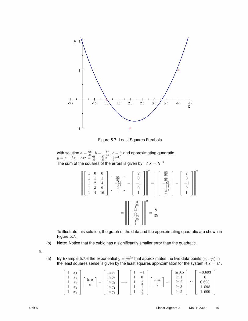
Figure 5.7: Least Squares Parabola

with solution a = 6835 , b = − 87

35 , c = 47 and approximating quadratic

y = a + bx + cx2 = 6835 − 87

35x + 47x2.

The sum of the squares of the errors is given by ‖AX −B‖2∥∥∥∥∥∥∥∥∥∥

1 0 01 1 11 2 41 3 91 4 16

6835− 87

3547

−

20−101

∥∥∥∥∥∥∥∥∥∥

2

=

∥∥∥∥∥∥∥∥∥∥

6835135− 26

35− 13

3587

−

20−101

∥∥∥∥∥∥∥∥∥∥

2

=

∥∥∥∥∥∥∥∥∥∥

− 235135935− 13

3517

∥∥∥∥∥∥∥∥∥∥

2

=835

To illustrate this solution, the graph of the data and the approximating quadratic are shown inFigure 5.7.

(b) Note: Notice that the cubic has a significantly smaller error than the quadratic.

9.

(a) By Example 5.7.6 the exponential y = aebx that approximates the five data points (xi, yi) inthe least squares sense is given by the least squares approximation for the system AX = B :

1 x1

1 x2

1 x3

1 x4

1 x5

[ln ab

]=

ln y1

ln y2

ln y3

ln y4

ln y5

=⇒

1 −11 01 1

21 11 3

2

[ln ab

]=

ln 0.5ln 1ln 2ln 3ln 5

'

−0.6930

0.6931. 0981. 609


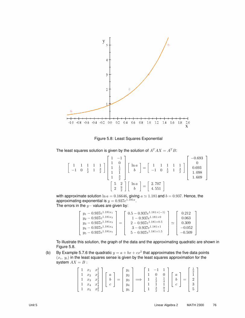
Figure 5.8: Least Squares Exponential

The least squares solution is given by the solution of AT AX = AT B:

[1 1 1 1 1−1 0 1

2 1 32

]

1 −11 01 1

21 11 3

2

[ln ab

]=

[1 1 1 1 1−1 0 1

2 1 32

]

−0.6930

0.6931. 0981. 609

[5 22 9

2

] [ln ab

]=

[2. 7074. 551

]

with approximate solution ln a = 0.16646, giving a ' 1.181 and b = 0.937. Hence, theapproximating exponential is y = 0.937e1.181x.The errors in the y− values are given by:

y1 − 0.937e1.181x1

y2 − 0.937e1.181x2

y3 − 0.937e1.181x3

y4 − 0.937e1.181x4

y5 − 0.937e1.181x5

=

0.5− 0.937e1.181×(−1)

1− 0.937e1.181×0

2− 0.937e1.181×0.5

3− 0.937e1.181×1

5− 0.937e1.181×1.5

'

0.2120.0630.309−0.052−0.509


(b) By Example 5.7.6 the quadratic y = a + bx + cx2 that approximates the five data points(xi, yi) in the least squares sense is given by the least squares approximation for thesystem AX = B :

1 x1 x21

1 x2 x22

1 x3 x23

1 x4 x24

1 x5 x25

abc

=

y1

y2

y3

y4

y5

=⇒

1 −1 11 0 01 1

214

1 1 11 3

294

abc

=

121235


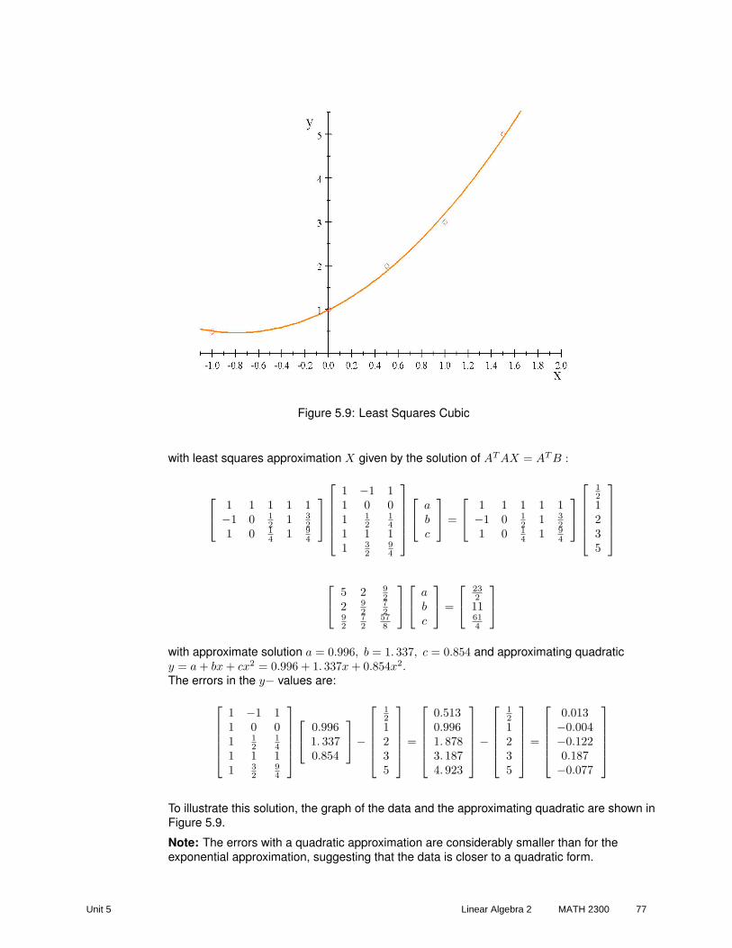
Figure 5.9: Least Squares Cubic

with least squares approximation X given by the solution of AT AX = AT B :

1 1 1 1 1−1 0 1

2 1 32

1 0 14 1 9

4

1 −1 11 0 01 1

214

1 1 11 3

294

abc

=

1 1 1 1 1−1 0 1

2 1 32

1 0 14 1 9

4

121235

5 2 92

2 92

72

92

72

578

abc

=

23211614

with approximate solution a = 0.996, b = 1. 337, c = 0.854 and approximating quadraticy = a + bx + cx2 = 0.996 + 1. 337x + 0.854x2.The errors in the y− values are:

1 −1 11 0 01 1

214

1 1 11 3

294

0.9961. 3370.854

−

121235

=

0.5130.9961. 8783. 1874. 923

−

121235

=

0.013−0.004−0.1220.187−0.077


Note: The errors with a quadratic approximation are considerably smaller than for theexponential approximation, suggesting that the data is closer to a quadratic form.


10. By Theorem 5.18 the projection p (x) = k1g1 (x) + k2g2 (x) + k3g3 (x) + k4g4 (x)

〈g1, g1〉〈g1, g2〉〈g1, g3〉〈g1, g4〉〈g2, g1〉〈g2, g2〉〈g2, g3〉〈g2, g4〉〈g3, g1〉〈g3, g2〉〈g3, g3〉〈g3, g4〉〈g4, g1〉〈g4, g2〉〈g4, g3〉〈g4, g4〉

k1

k2

k3

k4

=

〈g1, f〉〈g2, f〉〈g3, f〉〈g4, f〉

∫ 1

−11dx

∫ 1

−1xdx

∫ 1

−1x2dx

∫ 1

−1x3dx∫ 1

−1xdx

∫ 1

−1x2dx

∫ 1

−1x3dx

∫ 1

−1x4dx∫ 1

−1x2dx

∫ 1

−1x3dx

∫ 1

−1x4dx

∫ 1

−1x5dx∫ 1

−1x3dx

∫ 1

−1x4dx

∫ 1

−1x5dx

∫ 1

−1x6dx

k1

k2

k3

k4

=

∫ 1

−1exdx∫ 1

−1xexdx∫ 1

−1x2exdx∫ 1

−1x3exdx

2 0 23 0

0 23 0 2

523 0 2

5 00 2

5 0 27

k1

k2

k3

k4

=

2 sinh 12e−1

e− 5e−1

16e−1 − 2e

with approximate solution: k1 = 0.996, k2 = 0.998, k3 = 0.537, k4 = 0.176 and approximatingpolynomial:

y = 0.996 + 0.998x + 0.537x2 + 0.176x3

Note: The first four terms of the Taylor Series approximation to ex are:

ex ' 1 + x +12x2 +

16x3

' 1 + x + 0.5x2 + 0.167 x3

These values are reasonably close to those found by the least squares method.

11. Using the formulae for the means, x = 1m

∑x2, y = 1

m

∑y2 the simplified formula,

b =∑

(x−x)(y−y)∑(x−x)2

, numerator and denomenator are computed separately:

∑(x− x) (y − y) =

∑xy − x

∑y − y

∑x + xy

∑1

=∑

xy − 1m

∑x∑

y − 1m

∑y∑

x +1m

∑x× 1

m

∑y ×m

∑(x− x) (y − y) =

1m

(m

∑xy −

∑y∑

x)

∑(x− x)2 =

∑x2 − 2x

∑x + x2

∑1

=∑

x2 − 21m

∑x×

∑x +

(1m

∑x

)2

×m

∑(x− x)2 =

1m

(m

∑x2 −

(∑x)2

)

Hence the result follows:

b =∑

(x− x) (y − y)∑(x− x)2

=m

∑xy −

∑y∑

x

m∑

x2 −(∑

x)2 - the formula found in Exercise 5.7.5.

Starting with the simplified formula for a then:

y − bx = y −∑

(x− x) (y − y)∑(x− x)2

x

=y∑

(x− x)2 − x∑

(x− x) (y − y)∑(x− x)2


Computing the numerator separately:

= y∑

x2 − 2yx∑

x + yx2∑1− x∑

xy + x2∑y + xy∑

x− x2y∑

1

Moving the fourth term of the numerator up to the second position:

=1m

∑y∑

x2 − 1m

∑x∑

xy − 2myx× x + myx2 + mx2y + mxyx−mx2y

=1m

∑y∑

x2 −∑x∑

xy

Putting this back with the denomenator and using the formula for the denomenator derived above:

a =1m

∑y∑

x2 −∑x∑

xy∑(x− x)2

a =∑

y∑

x2 −∑x∑

xy

m∑

x2 −(∑

x)2 - the formula found in Exercise 5.7.5
