Underwater Acoustic MIMO OFDM:An experimental analysis

Guillem PalouAdvisor: Milica Stojanovic

Massachusetts Institute of Technology

September 2009

! " # $ %& %! %" %#!&'$

!&'#

!&'"

!&'!

&

&'!

&'"

&'#

()*+,-./012

34561-78509

Contents

List of Figures 4

Acknowledgements i

Resum iii

Abstract v

I Introduction 1

1 The Underwater Acoustic Channel 3

1.1 Attenuation . . . . . . . . . . . . . . . . . . . . . . . . . . . . . . . . . . 3

1.2 Noise . . . . . . . . . . . . . . . . . . . . . . . . . . . . . . . . . . . . . . 3

1.3 Multipath . . . . . . . . . . . . . . . . . . . . . . . . . . . . . . . . . . . 5

1.4 Doppler Effect . . . . . . . . . . . . . . . . . . . . . . . . . . . . . . . . . 5

2 Orthogonal Frequency Division Multiplexing 7

2.1 OFDM Signals . . . . . . . . . . . . . . . . . . . . . . . . . . . . . . . . 7

System . . . . . . . . . . . . . . . . . . . . . . . . . . . . . . . . . . . . . 7

Mathematical description . . . . . . . . . . . . . . . . . . . . . . . . . . . 8

Coding and Interleaving . . . . . . . . . . . . . . . . . . . . . . . . . . . 10

Advantages, Drawbacks and System Design . . . . . . . . . . . . . . . . 11

2.2 Intercarrier Interference . . . . . . . . . . . . . . . . . . . . . . . . . . . 12

Sources . . . . . . . . . . . . . . . . . . . . . . . . . . . . . . . . . . . . . 12

Signal model . . . . . . . . . . . . . . . . . . . . . . . . . . . . . . . . . . 13

3 MIMO Systems overview 15

3.1 Forms of MIMO . . . . . . . . . . . . . . . . . . . . . . . . . . . . . . . . 15

Single-Input Single-Output . . . . . . . . . . . . . . . . . . . . . . . . . . 15

Single-Input Multiple-Output . . . . . . . . . . . . . . . . . . . . . . . . 16

Multiple-Input Single Output . . . . . . . . . . . . . . . . . . . . . . . . 16

Multiple-Input Multiple-Output . . . . . . . . . . . . . . . . . . . . . . . 16

3.2 The MIMO channel . . . . . . . . . . . . . . . . . . . . . . . . . . . . . . 16

3.3 Space Time Coding . . . . . . . . . . . . . . . . . . . . . . . . . . . . . . 18

3.4 MIMO OFDM . . . . . . . . . . . . . . . . . . . . . . . . . . . . . . . . . 19

2

CONTENTS 3

II Data detection Algorithms 21

4 State of the Art of OFDM UWA Systems 23

Low-complexity OFDM detector . . . . . . . . . . . . . . . . . . . . . . . 23

Phase tracking . . . . . . . . . . . . . . . . . . . . . . . . . . . . 25

Channel Estimation . . . . . . . . . . . . . . . . . . . . . . . . . . 25

5 Adaptive Algorithm for MIMO systems 27

Channel estimation . . . . . . . . . . . . . . . . . . . . . . . . . . . . . . 28

Channel sparsing . . . . . . . . . . . . . . . . . . . . . . . . . . . 29

Channel estimated length . . . . . . . . . . . . . . . . . . . . . . 29

6 ICI Algorithms 31

6.1 Estimating the channel matrix . . . . . . . . . . . . . . . . . . . . . . . . 32

Pilot aided estimation . . . . . . . . . . . . . . . . . . . . . . . . . . . . 32

Adaptive Frequency Channel Estimator . . . . . . . . . . . . . . . . . . . 33

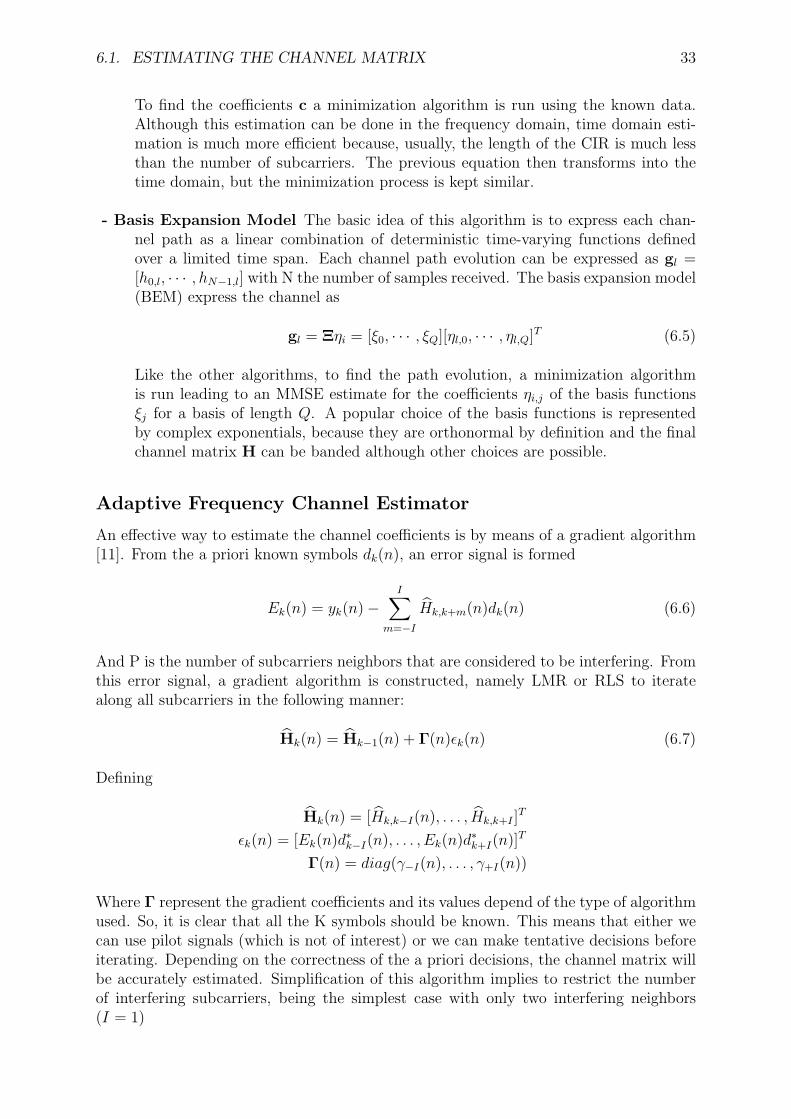
Frequency Domain - Decision Feedback Equalizer . . . . . . . . . . . . . 34

Taylor approximation . . . . . . . . . . . . . . . . . . . . . . . . . . . . . 35

6.2 Inverting the channel matrix . . . . . . . . . . . . . . . . . . . . . . . . . 36

LDLH Factorization . . . . . . . . . . . . . . . . . . . . . . . . . . . . . 36

LSQR Iterative method . . . . . . . . . . . . . . . . . . . . . . . . . . . . 37

Matrix Decoupling . . . . . . . . . . . . . . . . . . . . . . . . . . . . . . 38

Jacobi Stationary Iterative Method . . . . . . . . . . . . . . . . . . . . . 38

Matrix Simplification . . . . . . . . . . . . . . . . . . . . . . . . . . . . . 39

III Results and Conclusions 41

7 Results on experimental data 43

7.1 MIMO . . . . . . . . . . . . . . . . . . . . . . . . . . . . . . . . . . . . . 43

System description . . . . . . . . . . . . . . . . . . . . . . . . . . . . . . 43

Channel sparsing . . . . . . . . . . . . . . . . . . . . . . . . . . . . . . . 46

Phase Tracking & Doppler factor . . . . . . . . . . . . . . . . . . . . . . 47

MSE & BER . . . . . . . . . . . . . . . . . . . . . . . . . . . . . . . . . 51

Environmental correlation . . . . . . . . . . . . . . . . . . . . . . . . . . 52

7.2 ICI Compensation . . . . . . . . . . . . . . . . . . . . . . . . . . . . . . 52

Taylor approximation . . . . . . . . . . . . . . . . . . . . . . . . . . . . . 54

Compensation on SIMO systems . . . . . . . . . . . . . . . . . . . . . . . 54

8 Conclusions 59

Bibliography 61

List of Figures

1.1 Absorption coefficient in [dB/km] . . . . . . . . . . . . . . . . . . . . . . . . 4

1.2 Sources of ambient noise and analytical approximation . . . . . . . . . . . . 4

1.3 SNR depending on the frequency and transmission distance for a fixed trans-mitted power . . . . . . . . . . . . . . . . . . . . . . . . . . . . . . . . . . . 5

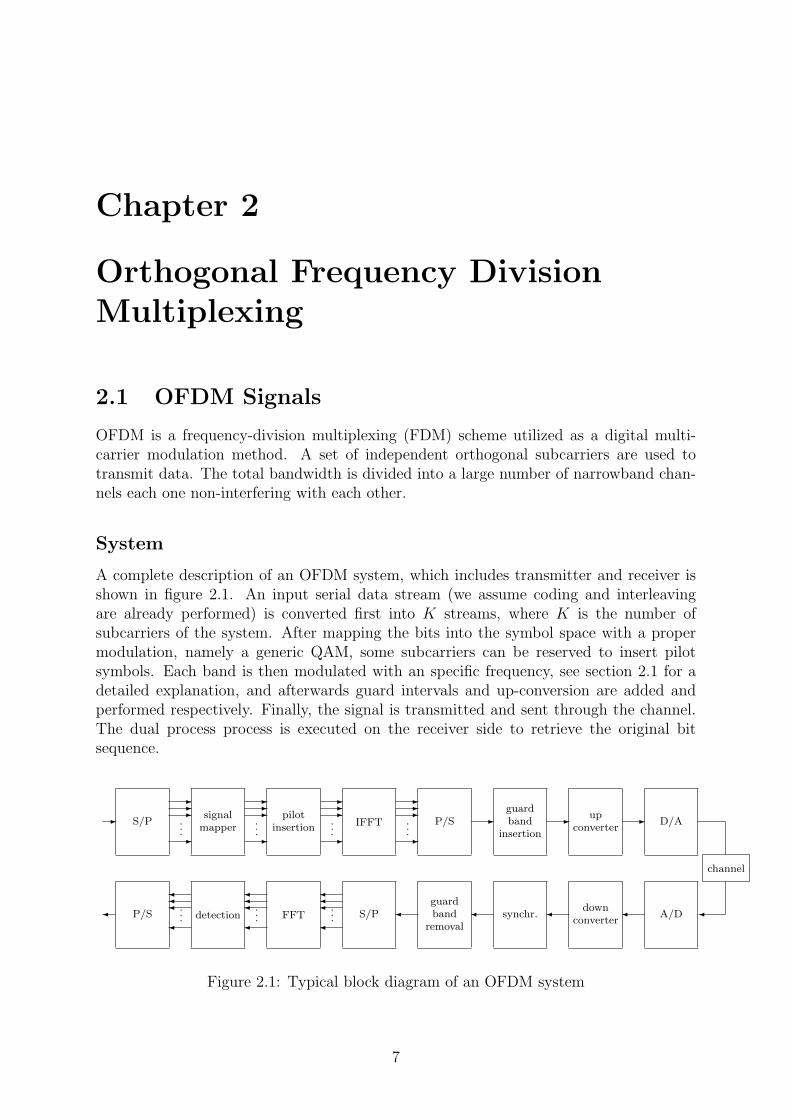
2.1 Typical block diagram of an OFDM system . . . . . . . . . . . . . . . . . . 7

2.2 OFDM Signal Spectrum with K = 128 subcarriers . . . . . . . . . . . . . . . 9

2.3 Example of time interleaving with the original and the interleaved data (topand bottom respectively). . . . . . . . . . . . . . . . . . . . . . . . . . . . . 11

2.4 Frequency synchronization in OFDM systems. . . . . . . . . . . . . . . . . . 12

2.5 Effect of the Doppler spread in the ICI phenomenon . . . . . . . . . . . . . . 13

3.1 Different forms of MIMO and their configuration . . . . . . . . . . . . . . . 16

3.2 Simplyfied scheme of the MIMO channel . . . . . . . . . . . . . . . . . . . . 17

4.1 Example of non-uniform Doppler shift . . . . . . . . . . . . . . . . . . . . . 24

4.2 Diagram of the algorithm described in [1] . . . . . . . . . . . . . . . . . . . . 24

6.1 Typical channel matrix for an ICI problem. Dark points mean highest coefficients 32

6.2 Scheme of a Frequency Domain DFE . . . . . . . . . . . . . . . . . . . . . . 34

6.3 Example of decoupling the diagonal of the channel matrix . . . . . . . . . . 38

7.1 Geometry of the experiment. . . . . . . . . . . . . . . . . . . . . . . . . . . 44

7.2 Wind speed with the wind direction indicated, wave height and wave periodduring the experiment. Stars mark the exact points in time when OFDMsignals were recorded. . . . . . . . . . . . . . . . . . . . . . . . . . . . . . . 45

7.3 Scatter plot for received QPSK and 8-PSK signals . . . . . . . . . . . . . . . 46

7.4 A typical channel impulse response. . . . . . . . . . . . . . . . . . . . . . . . 47

7.5 Channel Impulse Response estimated for a different number of threshold.From left to right and top to bottom: no sparsing, 10, 30, 60. . . . . . . . . 48

7.6 MSE and Coefficients kept (left to right) for a different number of sparsingthresholds . . . . . . . . . . . . . . . . . . . . . . . . . . . . . . . . . . . . . 48

7.7 Phases of three experiments with 128 and 1024 subcarriers and 1 transmitter. 49

7.8 Doppler of three experiments with 1024 subcarriers and 1 transmitter . . . . 49

7.9 Phases of three experiments with 1024 subcarriers and 2 transmitters . . . . 50

7.10 MSE for QPSK (top) and 8-PSK (bottom) for varying number of transmitters,MT=1, 2, 3 and 4 from left to right. . . . . . . . . . . . . . . . . . . . . . . 50

7.11 BER without coding for QPSK (top) and 8-PSK (bottom) for varying numberof transmitters, MT=1, 2, 3 and 4 from left to right. . . . . . . . . . . . . . 51

4

List of Figures 5

7.12 Wave height for the days of the experiment (top) and MSE (single transmitter,QPSK and 8-PSK, K=128, 256, 512, 1024). . . . . . . . . . . . . . . . . . . 53

7.13 Autocorrlation of a received signal (QPSK, K = 1024) after FFT demodulation. 547.14 Performance of ICI suppression on a QPSK signal set: linear equalization and

time-domain channel estimation based on Taylor series model are used. Thebackground light-grey curve corresponds to the ICI equalizer MSE. . . . . . 55

7.15 Scheme of ICI equalization prior to receiver combination . . . . . . . . . . . 557.16 Scheme of receiver combination before ICI suppression . . . . . . . . . . . . 567.17 Performance of ICI suppression on a SIMO system with a variable number of

receivers with EGC. . . . . . . . . . . . . . . . . . . . . . . . . . . . . . . . 577.18 Performance of ICI suppression on a SIMO system with a variable number of

receivers with MRC. . . . . . . . . . . . . . . . . . . . . . . . . . . . . . . . 57

Acknowledgements

I first would like to thank people who helped me to be able to do this work. Milica,as my advisor, helped me in all the problems and sugggestions I had. Her open mindshowed me how to look at the problems in many different ways, and try to solve them byseeking another perspective. I’m also thankful to MIT, specially the Sea Grant College,who offered me a lab and treated me like all the others in the team. My labmates in MIT,Jordi, Willy, Thang and Roman, were wonderful persons to share work with. Neverthe-less, regular meetings at Northeastern University, made the work more interesting, beingable to learn from other people, namely Ashish, Parastoo, Yashar, Rameez, Francesco,Baosheng and Joao.The work would have not be the same if life outside the laboratory didn’t exist. SpeciallyI would like to mention my roommate in the best house ever, 357 Columbia St., Jordi.Funny, intelligent and very... let’s say critic. I want to mention also other spanish peoplewho were present in my Bostonian life, Martin, Guillem, Hector, Miquel, Agua, Annawho was also my roommate; without them, I would have not been able to do it. Thanksto all.I would like to recognize my family for the sacrifice of missing me during all these months;and specially my girlfriend Alba, with whom I spent a whole month during the summer.She was all I needed during this period of time, she knew how I felt, she knew what todo; and now that it’s all over I don’t know how to thank her for all her effort. At least Ican put her name in this document. :)

i

Resum

Recentment, els esforcos de recerca han provat que el Multiplexat de Divisio Ortogonal enfrequencia (OFDM per les seves sigles en angles) representa una alternativa viable a lescomunicacions de portadora unica, que han estat utilitzades tradicionalment per enllacosde gran bitrate en entorns acustics submarins. La principal atraccio de l’OFDM es la sevasimplicitat en els processos de modulacio, demodulacio, implementats via FFT/IFFT.La recerca previa s’ha focalitzat en el disseny d’algorismes adaptatius que engloben totesles funcions necessaries de la capa fısica per un modem: sincronitzacio (adquisicio iniciali seguiment), estimacio del canal (tan el metode convencional com el dispers), detecciode les dades amb la seva corresponen decodificacio. Totes aquestes caracterıstiques ames d’utilitzar diversos receptors aixı com mes d’un transmissor per un enllac anomenatMIMO (Multiple-Input Multiple-Output) formen l’avantguarda de la nova generacio demodems subaquatics.Nomes recentment s’ha comencat a experimentar en entorns reals. OFDM ha estat am-pliament utilitzat en entorns radio, fins al punt d’estar inclos a diversos estandards del’IEEE. En comunicacions subaquatiques, aquesta tecnica de multiplexat en frequenciaes recent com per poder tenir resultats novedosos en aquest ambit. Donat que els primerstests experimentals van ser satisfactoris, la questio que es planteja ara es la dels lımits del’OFDM. L’objectiu d’aquest treball sera mesurar aquests lımits i veure si tenen algunarelacio amb les condicions fısiques o metorologiques, analitzant un seguit d’experimentsreals que van tenir lloc prop de la costa de Cape Cod.L’efficiencia d’un sistema MIMO-OFDM ve donada per R/B = mMT/(1 + TgB/K)bps/Hz, on m es el nivell de modulacio (els bits per sımbol, per ser mes concrets), MT

es el nombre d’elements transmissors, Tg es el temps de guarda que el sistema utilitzaentre dos blocks consecutius OFDM per evitar el multipath i que ha de ser mes llarg queel retard per multipropagacio del canal Tmp, B es l’ample de banda total que s’utilitza ifinalment K es el numero de subportadores que generalment es una potencia de 2 comara 128, 256... 1024. Com que els sistemes acustics estan limitats per banda a causade la gran atenuacio que sofreixen les altes frequencies, si es vol augmentar l’efficiencia,l’unic que es pot modificar son el numero de transmissors i les subportadores. Aquestsparametres, tanmateix, estan restringits tambe per la capacitat de processat i pel canalmateix. Una de les consideracions que s’assumeix en OFDM es que el canal resta invari-ant durant un block. Aleshores, incrementant el numero de subportadores (amb B fixe)resulta en un increment del temps de sımbol OFDM (T = K/B), cosa que possibilita alcanal variar la seva resposta durant aquest bloc. Mentre el temps de bloc estigui per sotadel temps de coherencia del canal no hi ha cap problema; en el moment que aquestes duesduracions son comparables, violem un dels principis d’estacionarietat de la FFT. Encaraque un processat post FFT pot compensar aquesta distorsio fins a un cert punt utilitzanttecniques de cancelacio de ICI (Inter-carrier Interference), una variacio del canal impor-tant pot causar perdues irrecuperables. L’unica manera de constrarestar aquest efecte

iii

iv RESUM

es mitjancant metodes pre-FFT; encara que utilitzant un processat mes complex redueixles avantatges de la simplicitat de l’OFDM. Aixı doncs, la variacio temporal del canalimposa un clar lımit a l’efficiencia d’un sistema OFDM en el numero de subportadoresque es poden arribar a utilitzar.El nombre d’elements transmissors que pot encabir un sistema esta limitat per la quanti-tat de conversa creuada (cross-talk en angles, efecte conegut per les les lınies telefoniquesanalogiques) que pot suportar l’estimador de canal MIMO. Es obvi que, com mes cross-talk hi hagi, mes dıficil sera la tasca de separar la informacio i aixı mes dıficil sera estimarel canal. Quantitativament, per que un receptor tingui suficients observacions per estimarMT respostes del canal, la llargada de cada una d’elles, L = dTmpBe, esta limitada perla condicio MT ≤ K/L. Aixo vol dir que si eventualment, donades el numero de sub-portadores i el nombre de transmissors, L es realment mes llarga que el que pot estimarel sistema, l’estimacio de canal no sera del tot correcta. Aixı, si establim un altre copl’equacio de l’eficiencia del sistema en funcio de la llargada del canal, trobem que aquestaeficiencia es, com a maxim, K2/(LK + L2) sımbols per segon i per Hertz.L’analisi experimental que s’ha dut a terme en aquest estudi es focalitza en senyalsacustiques enregistrades durant un perıode de 15 dies durant l’Octubre de 2008. L’experimentva ser realitzat al sud de l’illa Martha’s Vineyard a Cape Cod, Massachusetts. Un sistema4×12 MIMO va ser desplegat amb una distancia entre transmissors i receptors de 1000 men una profunditat de 15m a l’ocea Atlantic. Les condicions de l’experiment van resultarser molt variables, amb perıdodes de gran activitat d’onades i de forts vents. Les senyalsvan ser transmeses en la banda de 8 a 18 kHz (B = 10 kHz) i diversos parametres vananar variant-se, incloent diferents tipus de modulacio, com ara QPSK i 8-PSK, amb unrang de subportadores de 128 a 1024. Aquesta seleccio de parametres correspon a unaeficiencia espectral, sense codificar, de 0.9 a 10.4 bps/Hz. Aquest ampli rang ha permesposar a prova tant el sistema com el canal per a poder arribar a conclusions fermes.Les senyals han estat processades utilitzant un algoritme que incorpora una compen-sacio no uniforme de l’efecte Doppler. Com que la naturalesa fısica del sistema fa quesigui de banda ampla, la distorsio per efecte Doppler en una frequencia que en una al-tra. L’estimacio del canal MIMO ha estat realitzada utilitzant l’algoritme [2], el qualexplota de manera optima la coeherencia del canal en el domini frequencial. Els resul-tats obtinguts revelen (a) variacio del rendiment del sistema, que poden ser fins a unpunt deguts tambe a la variacio de les condicions meteorlogiques; (b) una millora delrendiment al augmentar el numero de subportadores per un nombre de transmissors de-terminat, fet que implica que el lımit imposat pel temps de coherencia no ha estat assolitamb les condicions presents; d’aquesta manera s’impulsa l’estimacio del canal ja que commes subportadores suporti el sistema, mes observacions per una correcta estimacio sondisponibles. Finalment, (c) el rendiment del sistema decreix quan s’augmenta el nombrede transmissors, cosa que, per altra banda, es d’esperar degut a l’increment de bitrate delsistema.

Abstract

Research efforts over the past several years have provided ample proof that orthogonalfrequency division multiplexing (OFDM) represents a viable alternative to single-carriermodulation which has traditionally been used for high rate communications over underwa-ter acoustic channels. The main attraction of OFDM lies in its simplicity of implementa-tion via FFT modulation/demodulation, which makes it a candidate for implementationin the next generation of acoustic modems.

Prior work has focused on the design and conceptual testing of adaptive detectionalgorithms that encompass all the necessary functions of the physical layer modem: syn-chronization (initial acquisition and continued tracking), channel estimation (conven-tional and sparse), and data detection and decoding; all in configuration with multiplereceive elements, as well as a single or multiple transmit elements. With successful com-pletion of initial field tests, a question naturally arises as to what are the limits of OFDMperformance. We address this question through an experimental analysis.

Bandwidth efficiency of MIMO OFDM is given as R/B = mMT/(1+TgB/K) bps/Hz,where m is the modulation level, MT is the number of transmit elements, Tg ≥ Tmp is aguard time greater than the multipath spread of the channel Tmp, B is the total systembandwidth, and K is the number of carriers. Since acoustic systems are bandwidth-limited, pushing the OFDM performance limits rests on increasing the number of carriersand transmit elements. These parameters, however, are restricted by the capabilities ofsignal processing and the channel itself. Specifically, increasing the number of carriersresults in an increased OFDM block duration (T = K/B), which in turn allows fora larger channel variation to occur over one block. The time-coherence assumption,necessary for FFT demodulation, is thus eventually violated. While a post-FFT processorcan compensate for some amount of time-variation by inter-carrier interference (ICI)cancellation, a larger variation will cause an irrecoverable loss during FFT demodulation.The only way in which this can be prevented is by pre-FFT processing; however, usinga more complex processor would diminish the original appeal of OFDM–its simplicity.Hence, the temporal variation of the channel imposes a fundamental limit on the numberof carriers K in a conventional OFDM system.

The number of transmit elements MT is limited by the amount of cross-talk that canbe handled by a MIMO channel estimator. In particular, in order for the receiver tohave a sufficient number of signal observations to estimate MT channel responses, eachof length L = dTmpBe, the number of transmitters has to be MT ≤ K/L. Hence, thebandwidth efficiency of a MIMO OFDM system is at most K2/(LK + L2) symbols persecond per Hertz.

Our experimental analysis focuses on acoustic signals recorded over a period of 15days during an October 2008 test conducted south of the island of Martha’s Vineyard inthe Atlantic Ocean. A 4 × 12 MIMO system was deployed over a 1 km range in about15 m of water. The conditions during the experiment were varying, with periods of high

v

vi ABSTRACT

wave activity. The signals, transmitted in the 8-18 kHz band (B=10 kHz), included4- and 8-PSK with varying number of carriers ranging between K=128 and 1024. Thisselection of signal parameters corresponds to a large range of bandwidth efficiencies, from0.9 to 10.4 bps/Hz.

The signals were processed using an adaptive algorithm that incorporates non-uniformDoppler compensation and sparse channel estimation. MIMO channel estimation was ac-complished using the algorithm [2], which optimally exploits channel coherence in thefrequency domain. These results reveal (a) performance variation over the course ofthe experiment, which can to some extent be correlated with the environmental con-dition; (b) performance improvement with an increase in the number of carriers for agiven number of transmit elements, which implies that the coherence limit is not reachedwithin the present conditions, thus boosting the decision-directed channel estimation byincreasing the number of signal observations in a block, and (c) performance decreasewith an increase in the number of transmit elements, which is to be expected given theaccompanying increase in the bit rate.

Part I

Introduction

1

Chapter 1

The Underwater Acoustic Channel

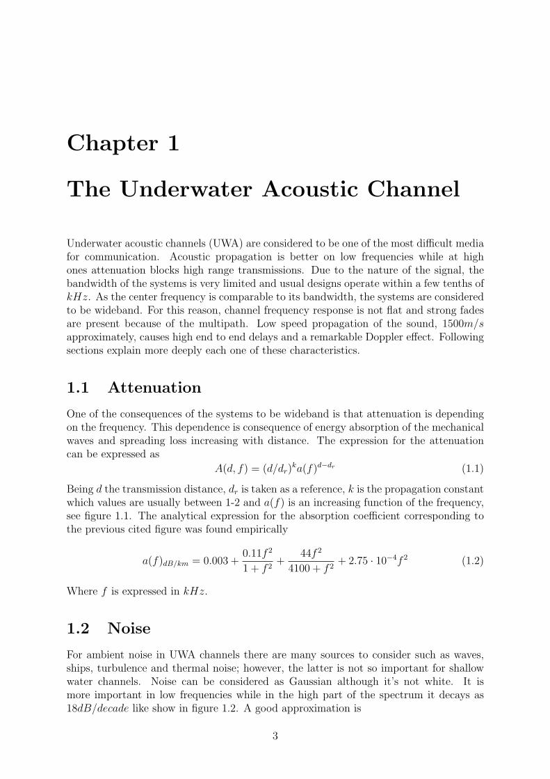
Underwater acoustic channels (UWA) are considered to be one of the most difficult mediafor communication. Acoustic propagation is better on low frequencies while at highones attenuation blocks high range transmissions. Due to the nature of the signal, thebandwidth of the systems is very limited and usual designs operate within a few tenths ofkHz. As the center frequency is comparable to its bandwidth, the systems are consideredto be wideband. For this reason, channel frequency response is not flat and strong fadesare present because of the multipath. Low speed propagation of the sound, 1500m/sapproximately, causes high end to end delays and a remarkable Doppler effect. Followingsections explain more deeply each one of these characteristics.

1.1 Attenuation

One of the consequences of the systems to be wideband is that attenuation is dependingon the frequency. This dependence is consequence of energy absorption of the mechanicalwaves and spreading loss increasing with distance. The expression for the attenuationcan be expressed as

A(d, f) = (d/dr)ka(f)d−dr (1.1)

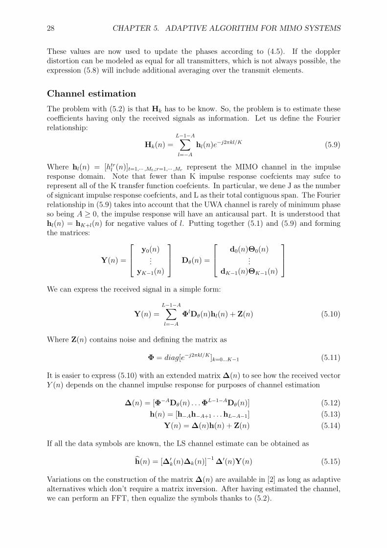
Being d the transmission distance, dr is taken as a reference, k is the propagation constantwhich values are usually between 1-2 and a(f) is an increasing function of the frequency,see figure 1.1. The analytical expression for the absorption coefficient corresponding tothe previous cited figure was found empirically

a(f)dB/km = 0.003 +0.11f 2

1 + f 2+

44f 2

4100 + f 2+ 2.75 · 10−4f 2 (1.2)

Where f is expressed in kHz.

1.2 Noise

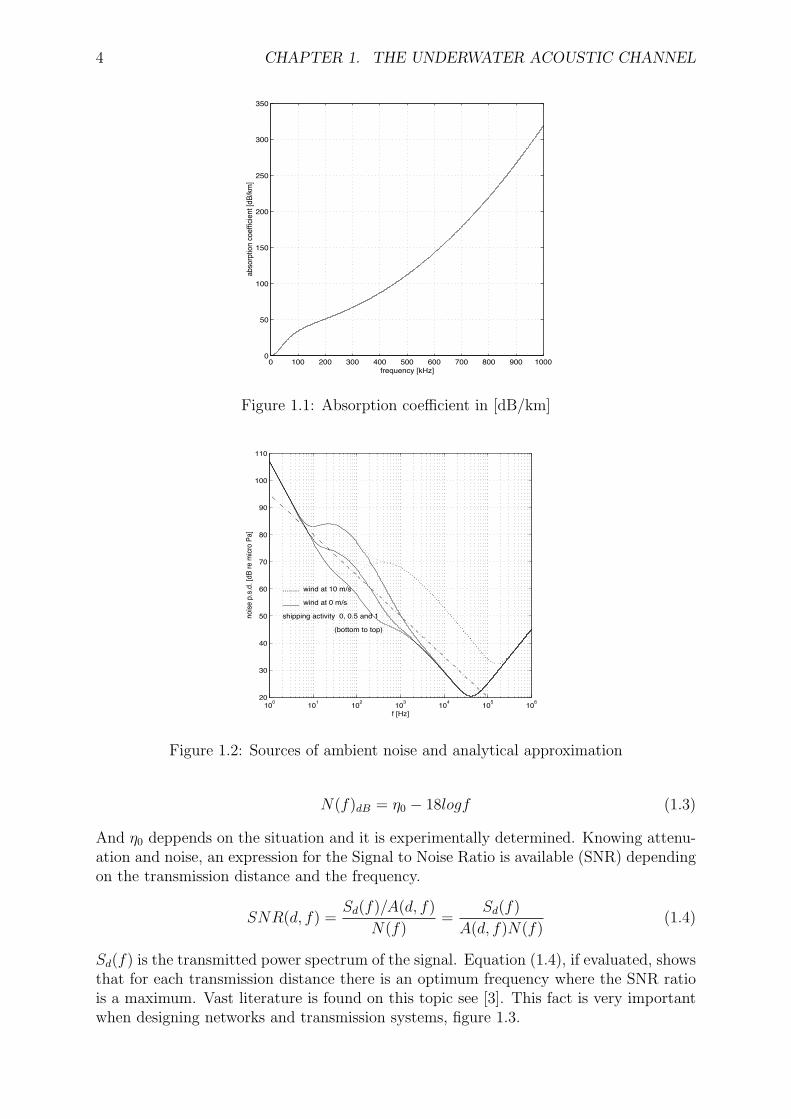
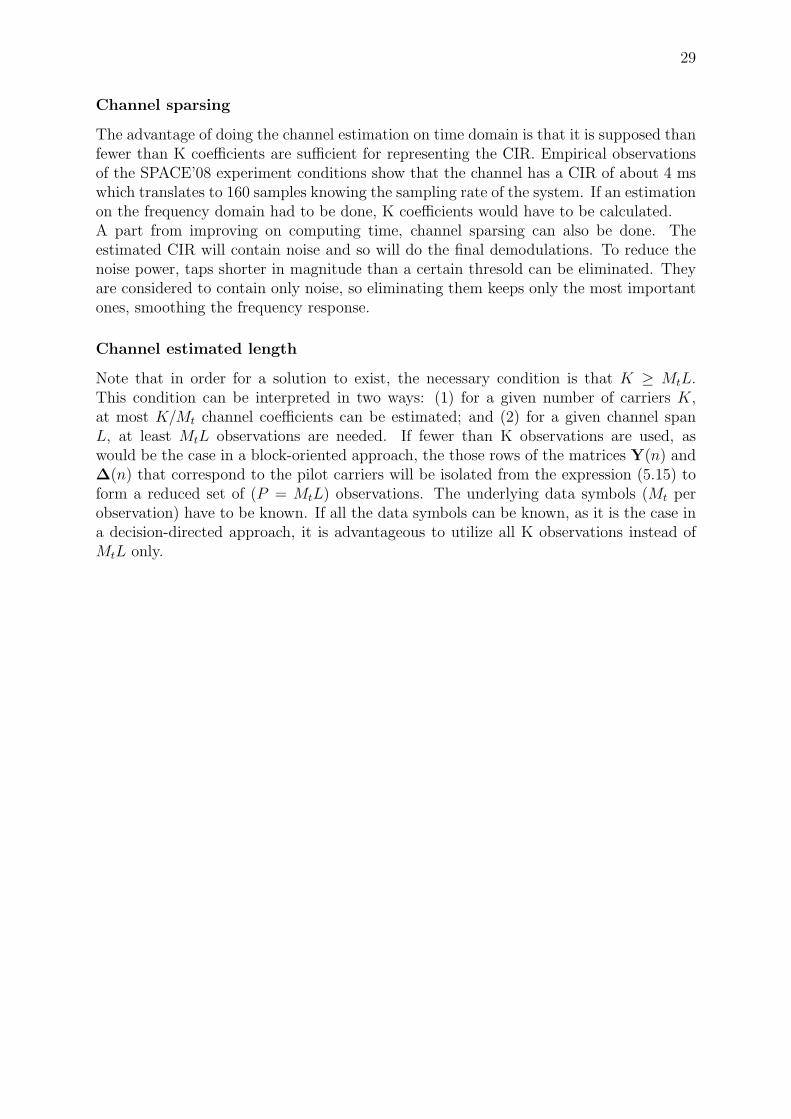
For ambient noise in UWA channels there are many sources to consider such as waves,ships, turbulence and thermal noise; however, the latter is not so important for shallowwater channels. Noise can be considered as Gaussian although it’s not white. It ismore important in low frequencies while in the high part of the spectrum it decays as18dB/decade like show in figure 1.2. A good approximation is

3

4 CHAPTER 1. THE UNDERWATER ACOUSTIC CHANNEL4 CHAPTER 1. UNDERWATER COMMUNICATIONS SYSTEMS

0 100 200 300 400 500 600 700 800 900 10000

50

100

150

200

250

300

350

frequency [kHz]

abso

rptio

n c

oeffic

ient [d

B/k

m]

Figure 1.1: Absorption coe!cient, a(f) [dB/km].

sources may be described as having a continuous spectrum and Gaussian statistics,with a power spectral density that decays at approximately 18dB/decade [2]. The ap-proximation is shown in Fig. 1.2. Site-specific noise is basically due to man-made noise,biological sources, ice cracking, rain and seismic events. For more detailed informationsee [3].

100

101

102

103

104

105

106

20

30

40

50

60

70

80

90

100

110

f [Hz]

nois

e p

.s.d

. [d

B r

e m

icro

Pa]

........ wind at 10 m/s

____ wind at 0 m/s

shipping activity 0, 0.5 and 1

(bottom to top)

Figure 1.2: Power spectral density of the ambient noise, N(f) [dB reµPa]. The dash-dot lineshows an approximation 10logN(f) = 50! 18logf .

From noise and attenuation, the signal-to-noise ratio (SNR) for a given bandwidthcan be computed. The bandwidth for a pre-specified SNR is severely limited at longerdistances. That is one of the reasons why multi-hop transmissions are better than directtransmissions (it also reduces the total transmitted power) [4]. At shorter distances,the available bandwidth will probably be limited by that of the transducer.

• Multipath

Figure 1.1: Absorption coefficient in [dB/km]

4 CHAPTER 1. UNDERWATER COMMUNICATIONS SYSTEMS

0 100 200 300 400 500 600 700 800 900 10000

50

100

150

200

250

300

350

frequency [kHz]abso

rptio

n c

oeffic

ient [d

B/k

m]

Figure 1.1: Absorption coe!cient, a(f) [dB/km].

sources may be described as having a continuous spectrum and Gaussian statistics,with a power spectral density that decays at approximately 18dB/decade [2]. The ap-proximation is shown in Fig. 1.2. Site-specific noise is basically due to man-made noise,biological sources, ice cracking, rain and seismic events. For more detailed informationsee [3].

100

101

102

103

104

105

106

20

30

40

50

60

70

80

90

100

110

f [Hz]

nois

e p

.s.d

. [d

B r

e m

icro

Pa]

........ wind at 10 m/s

____ wind at 0 m/s

shipping activity 0, 0.5 and 1

(bottom to top)

Figure 1.2: Power spectral density of the ambient noise, N(f) [dB reµPa]. The dash-dot lineshows an approximation 10logN(f) = 50! 18logf .

From noise and attenuation, the signal-to-noise ratio (SNR) for a given bandwidthcan be computed. The bandwidth for a pre-specified SNR is severely limited at longerdistances. That is one of the reasons why multi-hop transmissions are better than directtransmissions (it also reduces the total transmitted power) [4]. At shorter distances,the available bandwidth will probably be limited by that of the transducer.

• Multipath

Figure 1.2: Sources of ambient noise and analytical approximation

N(f)dB = η0 − 18logf (1.3)

And η0 deppends on the situation and it is experimentally determined. Knowing attenu-ation and noise, an expression for the Signal to Noise Ratio is available (SNR) dependingon the transmission distance and the frequency.

SNR(d, f) =Sd(f)/A(d, f)

N(f)=

Sd(f)

A(d, f)N(f)(1.4)

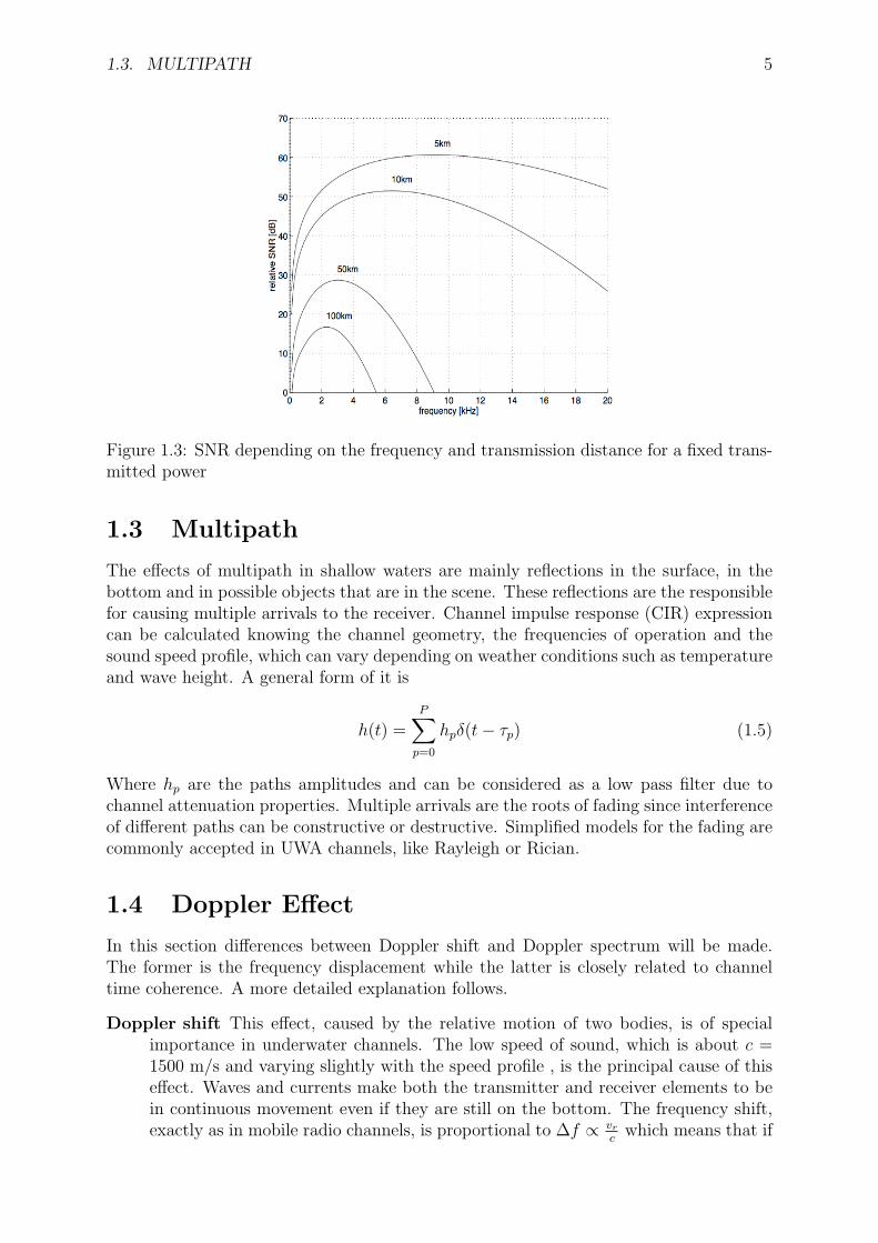
Sd(f) is the transmitted power spectrum of the signal. Equation (1.4), if evaluated, showsthat for each transmission distance there is an optimum frequency where the SNR ratiois a maximum. Vast literature is found on this topic see [3]. This fact is very importantwhen designing networks and transmission systems, figure 1.3.

1.3. MULTIPATH 5

Figure 1.3: SNR depending on the frequency and transmission distance for a fixed trans-mitted power

1.3 Multipath

The effects of multipath in shallow waters are mainly reflections in the surface, in thebottom and in possible objects that are in the scene. These reflections are the responsiblefor causing multiple arrivals to the receiver. Channel impulse response (CIR) expressioncan be calculated knowing the channel geometry, the frequencies of operation and thesound speed profile, which can vary depending on weather conditions such as temperatureand wave height. A general form of it is

h(t) =P∑p=0

hpδ(t− τp) (1.5)

Where hp are the paths amplitudes and can be considered as a low pass filter due tochannel attenuation properties. Multiple arrivals are the roots of fading since interferenceof different paths can be constructive or destructive. Simplified models for the fading arecommonly accepted in UWA channels, like Rayleigh or Rician.

1.4 Doppler Effect

In this section differences between Doppler shift and Doppler spectrum will be made.The former is the frequency displacement while the latter is closely related to channeltime coherence. A more detailed explanation follows.

Doppler shift This effect, caused by the relative motion of two bodies, is of specialimportance in underwater channels. The low speed of sound, which is about c =1500 m/s and varying slightly with the speed profile , is the principal cause of thiseffect. Waves and currents make both the transmitter and receiver elements to bein continuous movement even if they are still on the bottom. The frequency shift,exactly as in mobile radio channels, is proportional to ∆f ∝ vr

cwhich means that if

6 CHAPTER 1. THE UNDERWATER ACOUSTIC CHANNEL

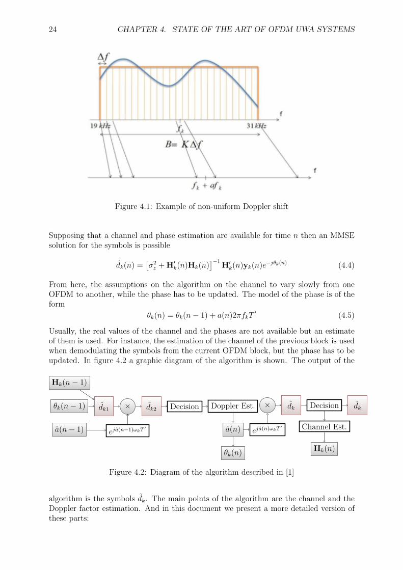
c, the wave propagation speed, is low then the shift will be higher. In mobile radiochannels shifts are of little interest in most of the cases, but in UWA channels thiseffect must be taken into account.One assumption on radio channel is that the Doppler shift is uniform all over thebandwidth. This is true, as the frequency shift is proportional also to the carrierfrequency, only if BW << fc. In UWA channels this approximation cannot befulfilled since the system bandwidth is comparable to its center carrier frequency.This leads then to non uniform Doppler shifts [4] and the signal spectrum expandsor contracts depending on the relative motion. As a consequence, the duration andbandwidth of the signal are not the same and new values are Td = T/(1 + a) andBd = B(1 + a) being a the Doppler factor.

Doppler spectrum The models behind Rayleigh or Rician fading assume that manywaves arrive each with its own random angle of arrival (thus with its own Dopplershift), which is uniformly distributed within [0...2π], independently of other waves.This allows to compute a probability density function of the frequency of incomingwaves. If we look at the Rayleigh fading channel in the time domain we find thatthe autocorrelation function of a specific tap (single arrival) is a first order Besselfunction which depends of the maximum Doppler spread. We then can calculatethe power spectral density (p.s.d.) of the Doppler, which shows how much thechannel spreads the signal. For example, If a sinusoidal signal is transmitted, aftertransmission over a fading channel, we will receive a power spectrum according toa U-shaped function

D(f) =1

2πfd

√1− ( f

fd)2|f | < fd (1.6)

Where fd is the maximum doppler spread. In practice, signals have a much complexspectrum but the frequency range where the power spectrum is nonzero defines theDoppler spread. This somehow is related to the channel time coherence. Morespecifically, as said before, the inverse Fourier transform of the Doppler spectrumis the autocorrelation function of a channel tap in time. From there, channel timecoherence tc can be inferred. Usual approximations assume that fd ∝ 1

tc.

Doppler effect is of extreme importance when dealing with multicarrier communications.Little frequency variations can cause an important degradation in performance. Usually,frequency shifts are corrected with hardware via resampling due to the cost of the oper-ation, while Doppler spectrum estimation can be done in a low-complexity manner oncehaving the sampled signals.

Chapter 2

Orthogonal Frequency DivisionMultiplexing

2.1 OFDM Signals

OFDM is a frequency-division multiplexing (FDM) scheme utilized as a digital multi-carrier modulation method. A set of independent orthogonal subcarriers are used totransmit data. The total bandwidth is divided into a large number of narrowband chan-nels each one non-interfering with each other.

System

A complete description of an OFDM system, which includes transmitter and receiver isshown in figure 2.1. An input serial data stream (we assume coding and interleavingare already performed) is converted first into K streams, where K is the number ofsubcarriers of the system. After mapping the bits into the symbol space with a propermodulation, namely a generic QAM, some subcarriers can be reserved to insert pilotsymbols. Each band is then modulated with an specific frequency, see section 2.1 for adetailed explanation, and afterwards guard intervals and up-conversion are added andperformed respectively. Finally, the signal is transmitted and sent through the channel.The dual process process is executed on the receiver side to retrieve the original bitsequence.

Chapter 2

Orthogonal Frequency DivisionMultiplexing

2.1 Introduction to OFDM

OFDM is a multicarrier transmission technique in which the available bandwidth is dividedamong many orthogonal carriers, and one symbol (of the same user) is transmitted in eachsubband. With this technique, a frequency selective channel is converted into several flatfading subchannels.

2.1.1 An OFDM system

The basic scheme of an OFDM system is given in Fig. 2.1.

! S/P

!...

!!! signal

mapper!...

!!! pilot

insertion!...

!!!

IFFT

!...

!!!

P/S !guardband

insertion

! upconverter

! D/A

channel

"" P/S"

...

"""

detection"

...

"""

FFT"

...

"""

S/P "guardband

removal

" synchr. " downconverter

" A/D

Figure 2.1: OFDM system: transmitter and receiver for CP-OFDM or ZP-OFDM-OLA.

The input data stream is serial-to-parallel converted into K streams dk(n), k = 0, ..., K!1, among which pilot tones are usually included to perform channel estimation at the receiver.K information symbols are transmitted in parallel on K carriers, creating an OFDM symbolwhose duration is K times greater than that of a single-carrier system. The guard bandinterval has to be long enough to accommodate for the delay spread, which helps to mitigatethe e!ect of the ISI caused by the channel multipath. It is called cyclic prefix (CP), if itis a copy of the last IFFT-precoded information samples added before the OFDM block, or

7

Figure 2.1: Typical block diagram of an OFDM system

7

8 CHAPTER 2. ORTHOGONAL FREQUENCY DIVISION MULTIPLEXING

Mathematical description

In this section a former description of the OFDM signals is shown. It is important to knowthat OFDM is formed by blocks each containing the transmission for the K subcarriers.Each block duration contains the effective symbol time and the guard interval

T = T ′ + Tg (2.1)

Where Tg stands for the guard time and it must be longer than channel impulse responselength to prevent inter-symbol interference between two consecutive OFDM blocks. T ′

stands for the effective symbol duration and it is defined as T ′ = B/K where B isthe overall system bandwidth and K is the number of subcarriers, the spacing betweenadjacent subcarriers is ∆f = 1/T ′. So, the subcarrier frequencies are:

fk = f0 + k∆f, k = 0 . . . K − 1, (2.2)

where f0 is the optional carrier frequency for a not baseband transmission. Each ofthe subcarriers contain a QAM symbol; typical modulations on the UWA channel areQPSK, 8PSK and low density QAM such as 16 or 32-QAM. It is assumed that all thesubcarriers contain the same modulation level; unlike the Discrete Multitone Modulation(DMT) where each subcarrier varies the bandwidth efficiency depending on the SNR inthat band.From the OFDM definition we can derive an expression for the bandwidth efficiency,which is the ratio for the bit rate to the bandwidth

R

B=

mα

1 + TgB/K(2.3)

Where m stands for the modulation level and its units are bits/symbol and for the case ofQPSK is m = 2 bits/symbol. α is the coding efficiency, either for block or convolutionalcoding. In (2.3) it is clearly seen that the efficiency of the system increases as spacingbetween subcarriers B/K and the guard interval decrease.Each one of the mapped symbols is modulated with one subcarrier, that is if the symbolon the k-subcarrier is called dk then the baseband expression of the modulated signal foronly one block is

bs(t) =K−1∑k=0

dkej2πk∆ft t = 0 . . . T ′ (2.4)

Equation (2.4) has the form of an IFFT operation. In fact, all the practical modulationschemes implement the OFDM modulation process as an IFFT due to its low-complexityand dedicated existing hardware. In the receiver side, an FFT will be key to retrievethe data. To transmit the signal, a guard interval must be added. This can be in theform of Cyclic Prefix (CP) or a simple Zero Padding (ZP) operation [5]. The first one isused in most of the radio systems for its capability to preserve the FFT/IFFT circularityconverting a linear channel convolution into a circular without any additional processingand offering good synchronization via autocorrelation on the receiver. The latter is usedwhen power saving is needed and it offers even better properties than CP, but additionalcomputations should be done to the received signal. The expressions for each one of the

2.1. OFDM SIGNALS 9

signals is given by

bs(t) =K−1∑k=0

dkej2πk∆ftgZP (t) t = 0 . . . T for ZP (2.5)

bs(t) =K−1∑k=0

dkej2πk∆f(t−Tg) t = 0 . . . T for CP (2.6)

The gZP (t) function is a rectangular pulse with duration T and it represents the zero-padding operation. Once known the baseband expression of the signal, the sent signalis

s(t) = <{bs(t)e

2πf0t}

(2.7)

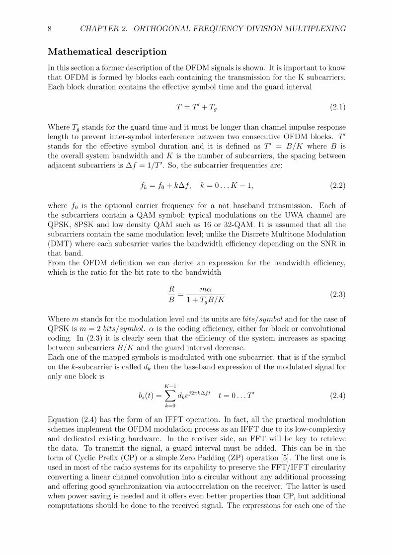
Therefore, s(t) represents an OFDM symbol containing K symbols. The spectrum of atypical OFDM signal is like the one shown in figure 2.3 The effective block symbol time is

0 0.05 0.1 0.15 0.2 0.25 0.3 0.35 0.4 0.45 0.510−5

10−4

10−3

10−2

10−1

100

101

Digital Frequency

Po

we

r

Figure 2.2: OFDM Signal Spectrum with K = 128 subcarriers

related to the subcarrier spacing to preserve the orthogonality between subcarriers. Thatis, for two specific subcarriers φk(t), φl(t) in the demodulator∫ T ′

0

φk(t)φl(t)∗ =

∫ T ′

0

ej2πk∆fte−j2πl∆ft = δ(k − l) (2.8)

Where δ(t) is the Kronecker’s delta. The orthogonality can be thought in time or infrequency domain. In time domain, as stated in previous equation, each subcarrier is asine wave with an integer number of cycles within a block so, the definition of a scalarproduct of two sine waves with multiple frequencies is zero. From the frequency domain,the spectrum of each subcarrier is a sinc function with its maximum value in its centerfrequency while being zero at other subcarriers’ centers.Although the modulation process is very simple, there are some practical mathematical

10 CHAPTER 2. ORTHOGONAL FREQUENCY DIVISION MULTIPLEXING

advices to be aware of. Let’s assume that the sampling frequency is fs and the number ofsamples of an OFDM block is Ns. When generating the signal in the frequency domain,an IFFT of at least 2K samples has to be done in order to verify the Nyquist theorem toprevent aliasing. Then a condition that must be satisfied always is Ns > 2K. Moreover,if the signal is translated to an upper band before D/A conversion, this condition has tobe more strict and becomes fs = Ns/T

′ > 2(f0 + ∆fK) = 2B.In the receiver side, accurate synchronization is needed. Whichever type of chosen OFDM,CP or ZP, the guard interval has to be removed prior to FFT demodulation. Synchro-nization and guard removal are processes that differ depending on the chosen scheme, [5]exposes them in a more detailed manner.

Coding and Interleaving

In order to keep the bit error rate probability low, or even an error free communication;coding and interleaving are needed to reduce incorrect detections. Usually, when usingan OFDM modulation, the system is considered wideband. Therefore, as the frequencyresponse of the channel is not equal for each subband, there can be parts of the spectrumwhich are more error prone due to their high attenuation and low SNR ratio. In thissection, an overview of some possibilities are outlined.

Coding Like in all other communications systems, in the useful bits that have to besent some redundancy is added. Channel coding, differenced to source or entropyencoding, is used to protect data sent over the channel even in the presence ofnoise. the redundancy added makes possible to retrieve the error-free original bitsif the coding is properly dimensioned. That is, depending on the SNR ratio, moreredundancy has to be applied. Shannon established a theoretical limit for the rateof the communications.

C = BW × log2(1 + SNR) bps (2.9)

The channel capacity, C, is directly proportional to the bandwidth used. Whendesigning a system the coding used has to respect this limit, if any knowledge ofprior SNR is available. Otherwise errors will appear on the receiver side.Two types of coding are mostly used in actual systems: block and convolutionalcoding. The main difference between them is that the former transforms blocks ofuseful bits into codewords properly designed while the output of the latter is formedbased on bit operations. To decode a block coding the received bits are assignedthe closest codeword and then retrieve the original bits. To decode a convolutionalcoding, the Viterbi algorithm is needed.

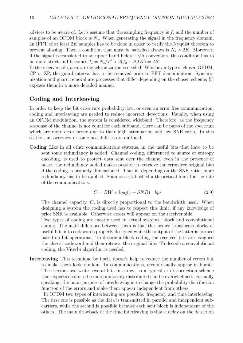
Interleaving This technique by itself, doesn’t help to reduce the number of errors butto make them look random. In communications, errors usually appear in bursts.These errors overwrite several bits in a row, so a typical error correction schemethat expects errors to be more uniformly distributed can be overwhelmed. Formallyspeaking, the main purpose of interleaving is to change the probability distributionfunction of the errors and make them appear independent from others.In OFDM two types of interleaving are possible: frequency and time interleaving.

The first one is possible as the data is transmitted in parallel and independent sub-carriers, while the second is possible because each sent block is independent of theothers. The main drawback of the time interleaving is that a delay on the detection

2.1. OFDM SIGNALS 11

Figure 2.3: Example of time interleaving with the original and the interleaved data (topand bottom respectively).

is introduced but as an advantage it protects the data from burst errors. Frequencyinterleaving is useful to deal with the non-flat channel frequency response so, errorwithin an OFDM also are more uniformly distributed with no delay expenses.

Advantages, Drawbacks and System Design

In this section the main advantages and drawbacks of an OFDM system.Advantages

• Can easily adapt to severe channel conditions without complex equalization

• Robust against narrow-band co-channel interference

• Robust against Intersymbol interference (ISI) and fading caused by multipath prop-agation

• High spectral efficiency

• Efficient implementation using FFT

• Low sensitivity to time synchronization errors

Drawbacks

• Sensitive to Doppler shift.

• Sensitive to frequency synchronization problems.

• High peak-to-average-power ratio (PAPR), requiring linear transmitter circuitry,which suffers from poor power efficiency.

• Loss of efficiency caused by Cyclic prefix/Guard interval.

Although there are some important factors in the drawbacks’ list, OFDM is the bestcandidate to support high rate underwater communications.

12 CHAPTER 2. ORTHOGONAL FREQUENCY DIVISION MULTIPLEXING

0

0.2

0.4

0.6

0.8

1

1.2

Frequency Domain

Spec

trum

Mag

nitud

e

Correct Frequency Synchronization Incorrect Frequency Synchronization

Figure 2.4: Frequency synchronization in OFDM systems.

2.2 Intercarrier Interference

One of the main causes of performance degradation is Intercarrier Interference (ICI). Themain advantage of OFDM is that each subcarrier is orthogonal, and thus independent,to each other. When the channel conditions change, this orthogonality disappears andthen, each subcarrier has some contribution to the others in the demodulating process.In this section, the sources of ICI are presented and a new OFDM signal model is alsoshown.

Sources

Although there can be many processed that can cause ICI here we will focus on the onesthat are more important in underwater communications.

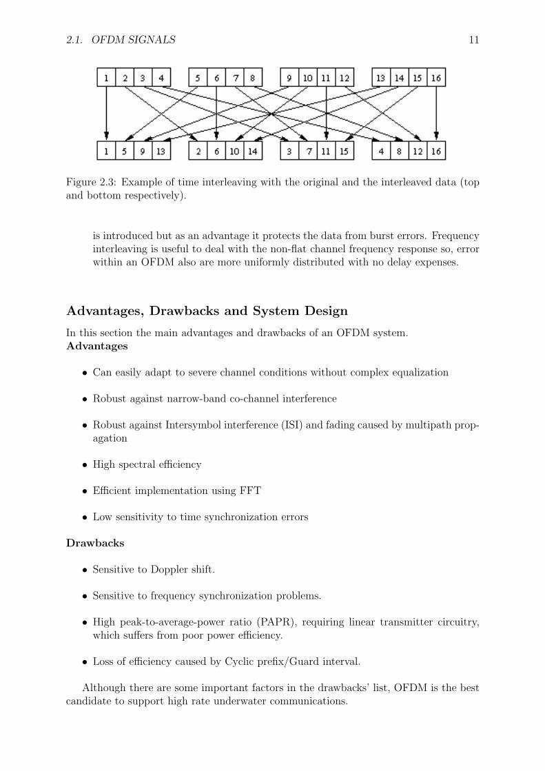
Doppler Shift As shown in section 1.4, the UWA channel suffers from severe Dopplereffect due to the low carrier frequencies and the low speed of propagation of sound.The main cause of this effect is the relative motion between the ends of the trans-mission. As a further matter, the wideband nature of the signal impacts in two waysin its transformation. A frequency shift, and a time (de)compression. Recall fromradio channels that time consequences are neglected in most of the cases and onlyfrequency shift is considered. When talking about wireless OFDM in UWA commu-nications it should be known that the Doppler shift can be sometimes comparableor even more than the subcarrier spacing. Conventionally, this shift is combatedvia resampling in time domain of the data, but its offset has to be known precisely.Produced ICI due to frequency de-synchronization is shown in figure 2.4. It canbe seen that if correct synchronization is performed, no influence of any subcarrieris collected (although the example only shows two subcarriers for clarity, this canbe extend to an arbitrary number). If the receiver oscillator has a little offset, orif there has been some uncorrected Doppler shift, incorrect synchronization is then

2.2. INTERCARRIER INTERFERENCE 13

0

0.2

0.4

0.6

0.8

1

1.2

Frequency Domain

Spec

trum

Mag

nitu

de

Influence of the adjacent subcarrier

Figure 2.5: Effect of the Doppler spread in the ICI phenomenon

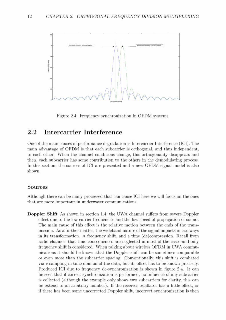
performed in the receiver and influence from other subcarriers are collected for oneband as shown with the red line in the figure.

Channel Time-Variance and Doppler Spread In OFDM, the channel is supposedto be time invariant within a block. If this condition is not satisfied, again, the sub-carriers loose their orthogonality. Mathematical expressions are available if someassumptions about the Doppler spread are maid [6]. Intuitively, figure 2.5 showshow this effect can lead to a degradation of the performance.Coherence time of the UWA channel is a critic paramter. Unlike radio communi-cations, the lack of high bandwidths can make a transmission of an OFDM blockwith a high number of subcarriers last for a few milliseconds. In this time, thechannel can change noticeably and time invariability is no longer respected. Inpractical situations, observations of the channel show that its coherence time canbe of about tc = 200 ms or less. As the Doppler spread fD is inversely proportionalrelated to tc, section 1.4, a spread of a few Hz is present in the system. There aresome real systems deployments which consider a subcarrier spacing of about 10Hz(a 1024-OFDM with 10KHz bandwidth, for example). Those system will suffer ofsevere ICI, if nothing is done about it.

Signal model

If ICI has to be considered, a more complex mathematical model arises. Although ana-lytical expressions can be derived making reasonable assumptions on the channel. Mostof the systems don’t need to be very accurate and simply model the received signal forone block as:

yk =K−1∑m=0

Hm,kdm + wk (2.10)

This simple model clearly shows that each received subband yk has the influence of allthe other subcarriers. Hm,k stands for the coefficient of the channel that represents the

14 CHAPTER 2. ORTHOGONAL FREQUENCY DIVISION MULTIPLEXING

influence of the subcarrier m to the subcarrier k and usually, in almost ICI-free systems,Hk,k >> Hm,k when m 6= k. A closed expression can also be found for the coefficientsHm,k in terms of the time variant CIR hn(l)

Hm,k =1

K

K−1∑n=0

L∑l=0

hn(l)exp

(j2π

n(m− k)−mlK

)(2.11)

If the channel impulse response hn(l) does not depend on the index n, only the coefficientsHk,k are non-zero and system is ICI free. This is however not real in practical systems.If we desire to simplify even more the model, we will simply separate the non-ICI partfrom the interfering one and lead to

yk = Hk,kdk + ICIk + wk (2.12)

The main drawback with this equation is that ICI is treated as additional noise. If itspower is negligible, this approximation can result in good performance without increasingsystem complexity, but if the power of the other subcarriers is somewhat important, thena more complex model, and yet a more complex system has to be taken into account, [6].

Chapter 3

MIMO Systems overview

MIMO, Multiple-Input Multiple-Output, is an antenna technology where multiple an-tennas are used in both ends of a transmission. Therefore, either in transmitter and/orreceiver more than one antenna is deployed. This technique allows to increase the bit rateof the communications link without need to increase the transmitter power per antennanor the bandwidth. These systems are defined by its spatial diversity and multiplexing,namely the number antennas used in both sides of the system.Spatial Multiplexing is defined as the transmission of multiple data streams over morethan one antenna. Two types have to be taken into consideration, V-BLAST (firstly usedin Bell Laboratories) and Space-Time Codes, which use orthogonal data streams for abetter detection on the receiver. See references for a more detailed informationSpatial Diversity is the source of improving channel capacity (multiplexing decreases it).The diversity is based on structured redundancy as the signal sent from one antenna isreceived in all the others. If the MIMO channel suffices some conditions, the system canretrieve the original sent signals from the received ones.

3.1 Forms of MIMO

Like many systems, MIMO exist in different forms as in figure 3.1. In the latest standards,such as the IEEE 802.11n or WiMAX, spatial diversity is used offering very good resultsin terms of capacity and bit rate. There are, though, many drawbacks of the techniqueand the number of transmitters is often limited to 4 in most of the standards. Thereare two main reasons, the first one is because each of the antennas has to be away ofthe other in order to make the received signal uncorrelated with the others, hence, moredeployed antennas mean a bigger transmitter and/or receiver. The second one is becauseof over-multiplexing and the MIMO channel, see section 3.2.

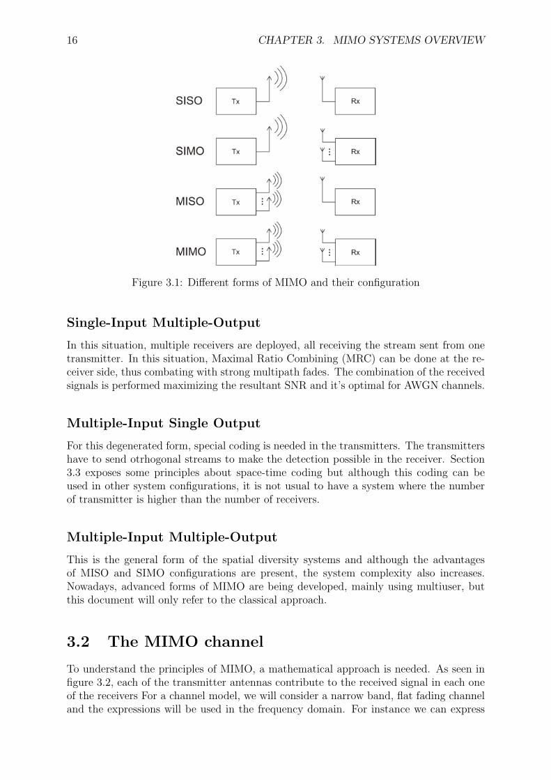
Single-Input Single-Output

This case cannot be considered an innovation scheme. The system is a conventionalcommunications system with one transmitter and one receiver. Nevertheless it is not ofless importance because nowadays there are still many systems that use this architecture.MIMO, for a proper behavior, needs multipath propagation to create a certain numberof uncorrelated and independent channels. In many situations, both transmitter andreceiver have a line of sight and little spatial diversity can be created.

15

16 CHAPTER 3. MIMO SYSTEMS OVERVIEW

Figure 3.1: Different forms of MIMO and their configuration

Single-Input Multiple-Output

In this situation, multiple receivers are deployed, all receiving the stream sent from onetransmitter. In this situation, Maximal Ratio Combining (MRC) can be done at the re-ceiver side, thus combating with strong multipath fades. The combination of the receivedsignals is performed maximizing the resultant SNR and it’s optimal for AWGN channels.

Multiple-Input Single Output

For this degenerated form, special coding is needed in the transmitters. The transmittershave to send otrhogonal streams to make the detection possible in the receiver. Section3.3 exposes some principles about space-time coding but although this coding can beused in other system configurations, it is not usual to have a system where the numberof transmitter is higher than the number of receivers.

Multiple-Input Multiple-Output

This is the general form of the spatial diversity systems and although the advantagesof MISO and SIMO configurations are present, the system complexity also increases.Nowadays, advanced forms of MIMO are being developed, mainly using multiuser, butthis document will only refer to the classical approach.

3.2 The MIMO channel

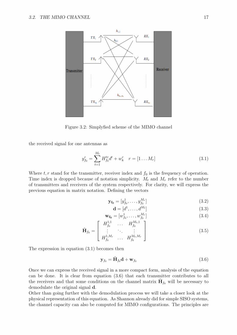
To understand the principles of MIMO, a mathematical approach is needed. As seen infigure 3.2, each of the transmitter antennas contribute to the received signal in each oneof the receivers For a channel model, we will consider a narrow band, flat fading channeland the expressions will be used in the frequency domain. For instance we can express

3.2. THE MIMO CHANNEL 17

Figure 3.2: Simplyfied scheme of the MIMO channel

the received signal for one antennas as

yrf0 =Mt∑t=1

H trf0dt + wrk r = [1 . . .Mr] (3.1)

Where t, r stand for the transmitter, receiver index and f0 is the frequency of operation.Time index is dropped because of notation simplicity. Mt and Mr refer to the numberof transmitters and receivers of the system respectively. For clarity, we will express theprevious equation in matrix notation. Defining the vectors

yf0 = [y1f0, . . . , yMr

f0] (3.2)

d = [d1, . . . , dMt ] (3.3)

wf0 = [w1f0, . . . , wMr

f0] (3.4)

Hf0 =

H1,1f0

. . . HMt,1f0

.... . .

...

H1,Mr

f0. . . HMt,Mr

f0

(3.5)

The expression in equation (3.1) becomes then

yf0 = Hf0d + wf0 (3.6)

Once we can express the received signal in a more compact form, analysis of the equationcan be done. It is clear from equation (3.6) that each transmitter contributes to allthe receivers and that some conditions on the channel matrix Hf0 will be necessary todemodulate the original signal d.Other than going further with the demodulation process we will take a closer look at thephysical representation of this equation. As Shannon already did for simple SISO systems,the channel capacity can also be computed for MIMO configurations. The principles are

18 CHAPTER 3. MIMO SYSTEMS OVERVIEW

the same, the capacity will be the maximum mutual information between the data beforethe channel, d and the data received, y. The usual expression for a flat fading channelis:

CMt,Mr = max{I(d,y)} = max EHf0{log2det

(IMt + Hf0RdH

′f0

)} (3.7)

Some considerations about the previous equation:

• If the channel is deterministic, the expected value is not used. If the channelrandom, averages are needed and then the term ergodic capacity is used

• The matrix Rdkrepresents the correlation of the sent bits. This matrix is mainly

the power allocation on the transmitters.

• Channel capacity is only useful in the transmitter side. Consequently, channel stateinformation (CSI) is needed at the transmission side of the communications system.

• If no CSI is available, no techniques on power allocation can be done, hence, thesame amount of power will be transmitted in each of the antennas.

• The strategy ot maximize the capacity depends on the type of fading assumed forthe channel. Rayleigh, Rician and Nakagami channels are the models used in typicalsituations.

Numerous studies have been done for the MIMO channel. This document will not focuson the statistical characterization of the UWA MIMO channel but more on demodulationtechniques that can be applied.

3.3 Space Time Coding

The Space Time Coding is a techniques used to improve reliability in a MIMO link.Redundancy is introduced in the transmitters with the hope that forward error correction(FEC) on the receiver will recover the original, useful data. Space time codes may bedivided into two subgroups:

Space Time Trellis Codes STTC Much complex than block codes, this types of codesdistribute a trellis code into several antennas thus providing diversity and codinggain. As the trellis coding is convolutional the receivers relies on the Viterbi algo-rithm to decode the data, thus increasing the system complexity.

Space Time Block Codes STBC This technique is based on constructing a set oforthogonal codewords which are transmitted along the antennas. the complexity ofit is much less that STTCs and only linear operations are needed.

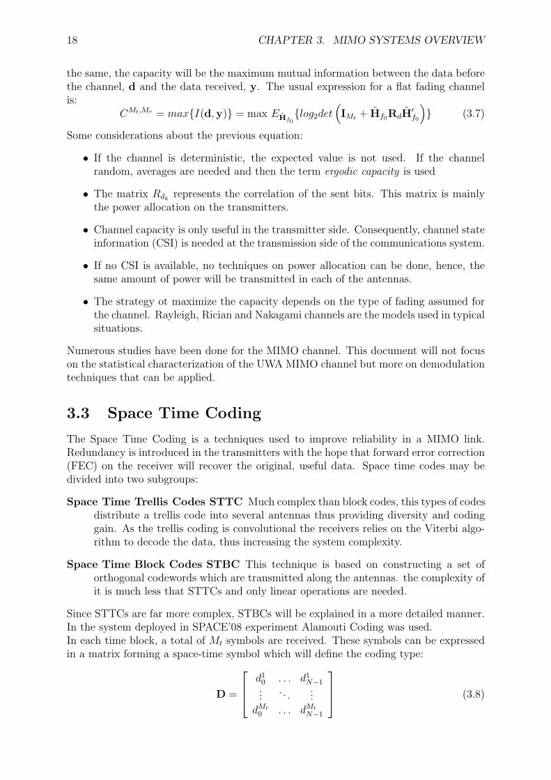
Since STTCs are far more complex, STBCs will be explained in a more detailed manner.In the system deployed in SPACE’08 experiment Alamouti Coding was used.In each time block, a total of Mt symbols are received. These symbols can be expressedin a matrix forming a space-time symbol which will define the coding type:

D =

d10 . . . d1

N−1...

. . ....

dMt0 . . . dMt

N−1

(3.8)

3.4. MIMO OFDM 19

Where dij represents the symbol sent on the transmitter i at time instant j. The mainpoint of the coding is to make the set of codewords, that is dij,∀i orthogonal betweeneach other. The result of this is simple, linear and optimal decoding at the receiver. Asmany coding techniques, the use of redundancy make the system sacrifice its data rate.The rate of the code is given by the number of encoded symbols in one time block (notethat many transmitters can send the same symbol) divided by the number of time slotsnecessary to complete the sapce-block symbol, r = #symbols/N . The simplest of thesecodes is the Alamouti’s code, with a matrix of 2× 2 with no bit rate loss as its rate is 1.The matrix for this code is

D =

[d1 d2

−d∗2 d∗1

](3.9)

Where it can be seen that the columns od the matrix are clearly orthogonal. In thereceiver side, using optimal decoding scheme, the bit-error rate (BER) behavior of theAlamouti’s code is equivalent to a MRC of 2 symbols over Mr receivers. This is aresult of the perfect orthogonality between the symbols after receive processing: thereare two copies of each symbol transmitted and Mr copies received. Maximum likelihooddecoding is performed with the only need of linear operations, thus maintaining thesystem complexity low. Recall that the symbols will not be recovered after 2 time slots(N for a general STBC) thus introducing a little delay.Although the commented scheme was for STBCs, STTCs are more robust against errors,but the receiver complexity is higher as dynamic programming algorithms are needed onthe receivers for correct data decoding. Either way, the use of space time coding permitsto MIMO systems to operate with more transmitters than receivers.

3.4 MIMO OFDM

When the MIMO channel was presented in previous sections, a flat fading model wasassumed. This is not true for a wideband system, where the channel has really differentresponses for each part of the spectrum. For instance, strong fades due to multipath cancause variations over 20 dB and the model for the MIMO capacity is no longer respected.One of the reasons why OFDM is a good associate for a MIMO transmission is because itdivides the overall spectrum into a set of narrow band, flat fading channels. This indeedcreates a group of independent channels, and each one of them accomplish the MIMOconditions presented before.The capacity is then the sum of each one of the narrow-band capacities. Obviously, if somesubband has less attenuation that others and a better SNR, a higher level modulation canbe employed in this band. Many wireless systems take profit of the subband independence,such as xDSL technologies, and transmit a different number of bits for each subband. Forthis to be possible CSI at the transmitter must be present. However in UWA channelsno feedback information from the receiver can be sent to the transmitter faster than thetime coherence of the channel, hence, uniform power allocation (UPA) and the same typeof modulation is used for all the subbands in OFDM.

Part II

Data detection Algorithms

21

Chapter 4

State of the Art of OFDM UWASystems

All along this chapter some of the existent algorithms for OFDM demodulation will beoutlined. Plenty of work has been done in this area since OFDM is a promising techniquefor high rate communications with wideband signals. UWA channels per se, are one ofthe most difficult channels for data transmission. Previous transmission techniques weretried for underwater communications such as spread spectrum or single carrier modula-tions for example. With the arrival of OFDM, the receiver and transmitter complexitydecreases achieving high efficiencies. Due to OFDM scalability the data rate can be var-ied significantly so, each communication link can be tuned easily to have the maximumpossible bit rate.The purpoes of this document is to apply one algorithm for a MIMO system with dataof the SPACE’08 experiment and see the results. Additionally, some ideas about ICI areconsidered.

Low-complexity OFDM detector

This algorithm, in contraposition with the previous one, makes all the processing postFFT. The technique in [4] dealt with the resampling frequency and modified the signalbefore the FFT operation. Although the Doppler shifts that can be corrected via hardwareare higher than the ones only using software, its simplicity makes it worth mentioning.The algorithm in [1] makes uses of multiple receiver MMSE combining and separes phasetracking from equalization using a Doppler model for the phase change, see figure 4.1.Let’s define the received signal vector for a given subband

yk(n) =[y0k(n) . . . yMr

k (n)]

(4.1)

Where the expression of each received signal yrk(n) for receiver r and OFDM block indexn can be seen as

yrk(n) = Hrk(n)dke

jθk(n) + zk(n) (4.2)

Where Hk is the frequency response of the channel at the subband k for 0 ≥ k < K. Theterm θk(n) is the time-varying phase offset. The matrix notation for all the receivers is

yk(n) = Hk(n)dkejθk(n) + zk(n) (4.3)

23

24 CHAPTER 4. STATE OF THE ART OF OFDM UWA SYSTEMS

Figure 4.1: Example of non-uniform Doppler shift

Supposing that a channel and phase estimation are available for time n then an MMSEsolution for the symbols is possible

dk(n) =[σ2z + H′k(n)Hk(n)

]−1H′k(n)yk(n)e−jθk(n) (4.4)

From here, the assumptions on the algorithm on the channel to vary slowly from oneOFDM to another, while the phase has to be updated. The model of the phase is of theform

θk(n) = θk(n− 1) + a(n)2πfkT′ (4.5)

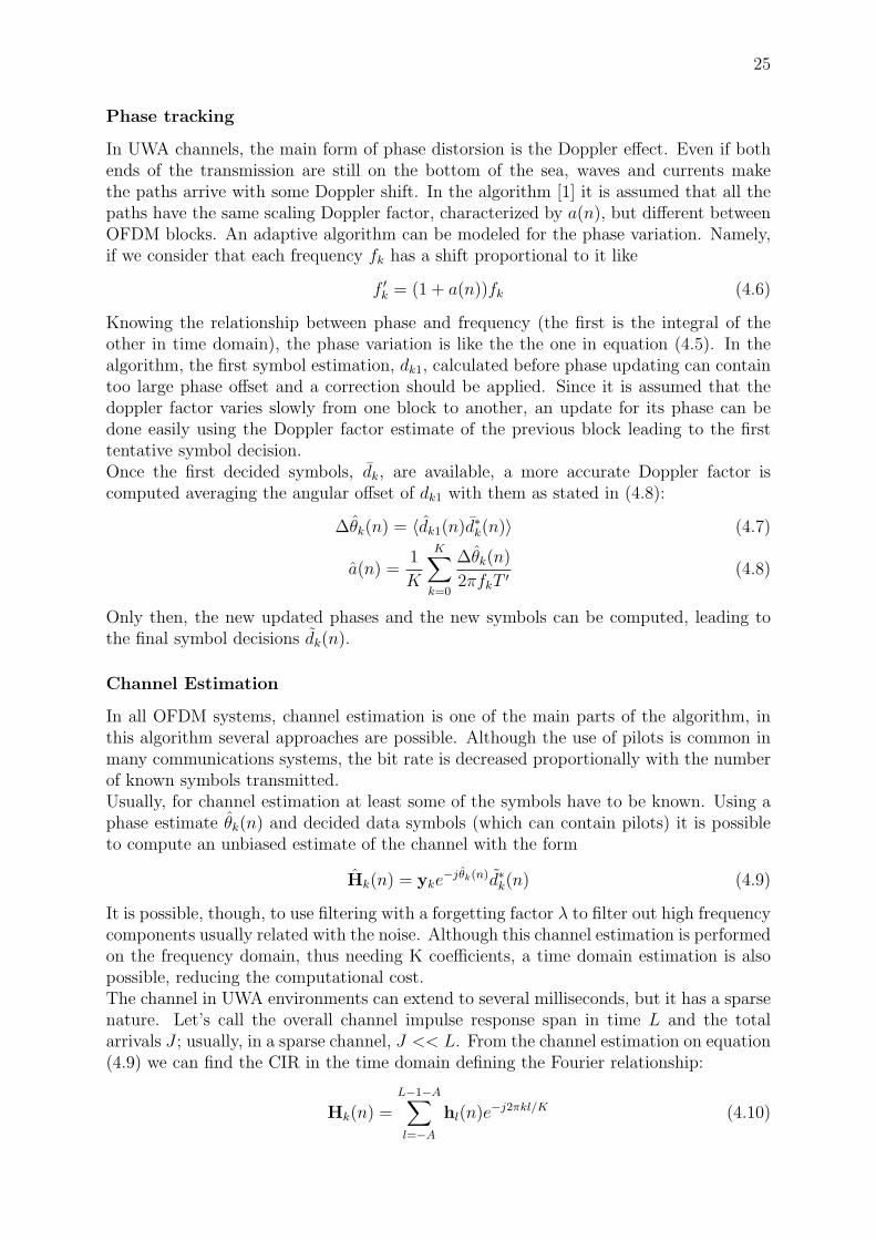
Usually, the real values of the channel and the phases are not available but an estimateof them is used. For instance, the estimation of the channel of the previous block is usedwhen demodulating the symbols from the current OFDM block, but the phase has to beupdated. In figure 4.2 a graphic diagram of the algorithm is shown. The output of the

Hk(n− 1)

θk(n− 1)

a(n− 1)

dk1 ×

eja(n−1)ωkT′

dk2 Decision Doppler Est.

a(n)

θk(n)

eja(n)ωkT′

× dk Decision

Channel Est.

Hk(n)

dk

Figure 4.2: Diagram of the algorithm described in [1]

algorithm is the symbols dk. The main points of the algorithm are the channel and theDoppler factor estimation. And in this document we present a more detailed version ofthese parts:

25

Phase tracking

In UWA channels, the main form of phase distorsion is the Doppler effect. Even if bothends of the transmission are still on the bottom of the sea, waves and currents makethe paths arrive with some Doppler shift. In the algorithm [1] it is assumed that all thepaths have the same scaling Doppler factor, characterized by a(n), but different betweenOFDM blocks. An adaptive algorithm can be modeled for the phase variation. Namely,if we consider that each frequency fk has a shift proportional to it like

f ′k = (1 + a(n))fk (4.6)

Knowing the relationship between phase and frequency (the first is the integral of theother in time domain), the phase variation is like the the one in equation (4.5). In thealgorithm, the first symbol estimation, dk1, calculated before phase updating can containtoo large phase offset and a correction should be applied. Since it is assumed that thedoppler factor varies slowly from one block to another, an update for its phase can bedone easily using the Doppler factor estimate of the previous block leading to the firsttentative symbol decision.Once the first decided symbols, dk, are available, a more accurate Doppler factor iscomputed averaging the angular offset of dk1 with them as stated in (4.8):

∆θk(n) = 〈dk1(n)d∗k(n)〉 (4.7)

a(n) =1

K

K∑k=0

∆θk(n)

2πfkT ′(4.8)

Only then, the new updated phases and the new symbols can be computed, leading tothe final symbol decisions dk(n).

Channel Estimation

In all OFDM systems, channel estimation is one of the main parts of the algorithm, inthis algorithm several approaches are possible. Although the use of pilots is common inmany communications systems, the bit rate is decreased proportionally with the numberof known symbols transmitted.Usually, for channel estimation at least some of the symbols have to be known. Using aphase estimate θk(n) and decided data symbols (which can contain pilots) it is possibleto compute an unbiased estimate of the channel with the form

Hk(n) = yke−jθk(n)d∗k(n) (4.9)

It is possible, though, to use filtering with a forgetting factor λ to filter out high frequencycomponents usually related with the noise. Although this channel estimation is performedon the frequency domain, thus needing K coefficients, a time domain estimation is alsopossible, reducing the computational cost.The channel in UWA environments can extend to several milliseconds, but it has a sparsenature. Let’s call the overall channel impulse response span in time L and the totalarrivals J ; usually, in a sparse channel, J << L. From the channel estimation on equation(4.9) we can find the CIR in the time domain defining the Fourier relationship:

Hk(n) =L−1−A∑l=−A

hl(n)e−j2πkl/K (4.10)

26 CHAPTER 4. STATE OF THE ART OF OFDM UWA SYSTEMS

Note that an UWA channel is rarely of minimum phase thus having arrivals before thestrongest path. This means that the direct path between transmitter and receiver is notthe fastest one, unlike the radio channel if a line of sight is available. After performingthe IFFT, coefficients below a certain threshold γ can be eliminated as the channel willcontain also noise and eliminating low energy taps can also reduce the noise variance.Thus, the channel CIR will be

hl(n) =

{hl(n) if |hl(n)| > γ

0 if |hl(n)| ≤ γ(4.11)

Different results are obtained for different γ, see section 7 for more details. Normally,γ is defined as γ = ρ×max(|hl(n)|) where ρ is between 0 and 1The MIMO algorithm explained later in section 5 will use many of the equations shownin this section. In a simplified manner, the adaptation of this algorithm to multiple trans-mitters implies tracking of several Doppler factors, one for each transmitter, and a moredifficult channel estimation because each pair of transmitter and receiver hydrophoneshas his own channel.

Chapter 5

Adaptive Algorithm for MIMOsystems

The receiver algorithm used for data detection in the SPACE’08 experiment is the oneexplained in [2] and an overview is presented here commenting also the particularities ofthe MIMO channel. As a result of sending the signal through a channel, the receivedsignal can be expressed in the frequency domain after the FFT demodulation as

yrk(n) =Mt∑t=0

H trk (n)dtk(n)ejθ

tk(n) + ntk(n) (5.1)

Where t, r, k, n refer to the transmitter, the receiver the frequency index and the timerespectively. H is referring to the channel frequency response and n to the noise compo-nent of the received signal. Using the expression (5.1) it is possible to construct an LSestimate of the received symbols in a matrix form:

dk1(n) = yk(n)H′k(n) [Hk(n)H′k(n)]−1

Θ∗k(n) (5.2)

The prime denotes hemitian transpose and the asterisk complex conjugate. In practice,when the channels and the phases are not known, their estimates will be used instead oftrue values in the expression 5.2. Symbol decisions can then be made, e.g. by soft-decisiondecoding. Matrices and the vectors appearing in (5.2) are defined as

yk(n) = [y1k(n) . . . yMr

k (n)] (5.3)

dk1(n) = [d1k(n) . . . dMt

k (n)] (5.4)

Hk(n) = [H trk (n)]t=1···Mt;r=1···Mr (5.5)

Θk(n) = diag[ejθtk(n)]t=1···Mt (5.6)

The existing channel estimate Hk(n − 1) is used to form two types of symbol estimatesaccording to the expression (5.2): dk(n) is obtained using the predicted phase θtk(n) and

dk(n) is obtained using the outdated phase θtk(n). The former is used to make tentativesymbol decisions dk(n), as the latter may contain too large phase offset. The underlyingphase error is measured as

ψtk(n) = 〈dtk(n)dt∗k (n)〉,∀k, t (5.7)

And used to update the Doppler factors by averaging

at(n) =1

K

K−1∑k=0

ψtk(n)

2πfkT ′(5.8)

27

28 CHAPTER 5. ADAPTIVE ALGORITHM FOR MIMO SYSTEMS

These values are now used to update the phases according to (4.5). If the dopplerdistortion can be modeled as equal for all transmitters, which is not always possible, theexpression (5.8) will include additional averaging over the transmit elements.

Channel estimation

The problem with (5.2) is that Hk has to be know. So, the problem is to estimate thesecoefficients having only the received signals as information. Let us define the Fourierrelationship:

Hk(n) =L−1−A∑l=−A

hl(n)e−j2πkl/K (5.9)

Where hl(n) = [htrl (n)]t=1,··· ,Mt,;r=1,··· ,Mr represent the MIMO channel in the impulseresponse domain. Note that fewer than K impulse response coefcients may sufce torepresent all of the K transfer function coefcients. In particular, we dene J as the numberof signicant impulse response coefcients, and L as their total contiguous span. The Fourierrelationship in (5.9) takes into account that the UWA channel is rarely of minimum phaseso being A ≥ 0, the impulse response will have an anticausal part. It is understood thathl(n) = hK+l(n) for negative values of l. Putting together (5.1) and (5.9) and formingthe matrices:

Y(n) =

y0(n)...

yK−1(n)

Dθ(n) =

d0(n)Θ0(n)...

dK−1(n)ΘK−1(n)

We can express the received signal in a simple form:

Y(n) =L−1−A∑l=−A

ΦlDθ(n)hl(n) + Z(n) (5.10)

Where Z(n) contains noise and defining the matrix as

Φ = diag[e−j2πkl/K ]k=0...K−1 (5.11)

It is easier to express (5.10) with an extended matrix ∆(n) to see how the received vectorY (n) depends on the channel impulse response for purposes of channel estimation

∆(n) = [Φ−ADθ(n) . . .ΦL−1−ADθ(n)] (5.12)

h(n) = [h−Ah−A+1 . . .hL−A−1] (5.13)

Y(n) = ∆(n)h(n) + Z(n) (5.14)

If all the data symbols are known, the LS channel estimate can be obtained as

h(n) = [∆′k(n)∆k(n)]−1

∆′(n)Y(n) (5.15)

Variations on the construction of the matrix ∆(n) are available in [2] as long as adaptivealternatives which don’t require a matrix inversion. After having estimated the channel,we can perform an FFT, then equalize the symbols thanks to (5.2).

29

Channel sparsing

The advantage of doing the channel estimation on time domain is that it is supposed thanfewer than K coefficients are sufficient for representing the CIR. Empirical observationsof the SPACE’08 experiment conditions show that the channel has a CIR of about 4 mswhich translates to 160 samples knowing the sampling rate of the system. If an estimationon the frequency domain had to be done, K coefficients would have to be calculated.A part from improving on computing time, channel sparsing can also be done. Theestimated CIR will contain noise and so will do the final demodulations. To reduce thenoise power, taps shorter in magnitude than a certain thresold can be eliminated. Theyare considered to contain only noise, so eliminating them keeps only the most importantones, smoothing the frequency response.

Channel estimated length

Note that in order for a solution to exist, the necessary condition is that K ≥ MtL.This condition can be interpreted in two ways: (1) for a given number of carriers K,at most K/Mt channel coefficients can be estimated; and (2) for a given channel spanL, at least MtL observations are needed. If fewer than K observations are used, aswould be the case in a block-oriented approach, the those rows of the matrices Y(n) and∆(n) that correspond to the pilot carriers will be isolated from the expression (5.15) toform a reduced set of (P = MtL) observations. The underlying data symbols (Mt perobservation) have to be known. If all the data symbols can be known, as it is the case ina decision-directed approach, it is advantageous to utilize all K observations instead ofMtL only.

Chapter 6

ICI Algorithms

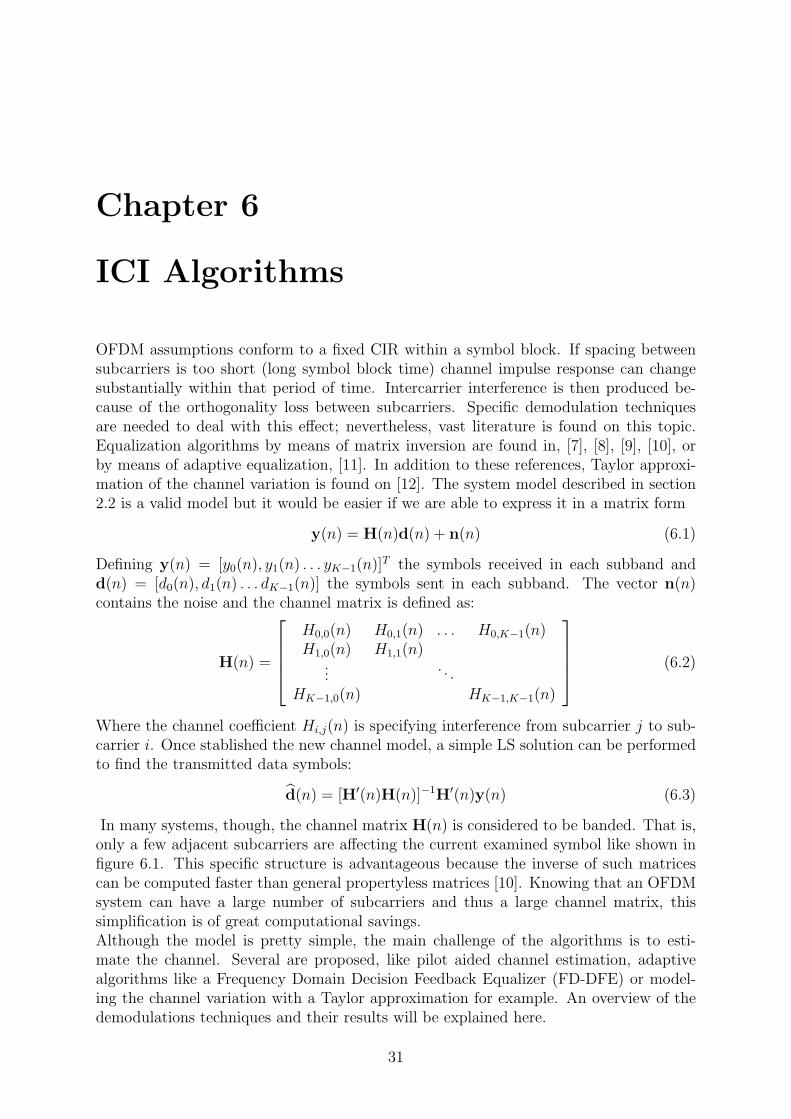
OFDM assumptions conform to a fixed CIR within a symbol block. If spacing betweensubcarriers is too short (long symbol block time) channel impulse response can changesubstantially within that period of time. Intercarrier interference is then produced be-cause of the orthogonality loss between subcarriers. Specific demodulation techniquesare needed to deal with this effect; nevertheless, vast literature is found on this topic.Equalization algorithms by means of matrix inversion are found in, [7], [8], [9], [10], orby means of adaptive equalization, [11]. In addition to these references, Taylor approxi-mation of the channel variation is found on [12]. The system model described in section2.2 is a valid model but it would be easier if we are able to express it in a matrix form

y(n) = H(n)d(n) + n(n) (6.1)

Defining y(n) = [y0(n), y1(n) . . . yK−1(n)]T the symbols received in each subband andd(n) = [d0(n), d1(n) . . . dK−1(n)] the symbols sent in each subband. The vector n(n)contains the noise and the channel matrix is defined as:

H(n) =

H0,0(n) H0,1(n) . . . H0,K−1(n)H1,0(n) H1,1(n)

.... . .

HK−1,0(n) HK−1,K−1(n)

(6.2)

Where the channel coefficient Hi,j(n) is specifying interference from subcarrier j to sub-carrier i. Once stablished the new channel model, a simple LS solution can be performedto find the transmitted data symbols:

d(n) = [H′(n)H(n)]−1H′(n)y(n) (6.3)

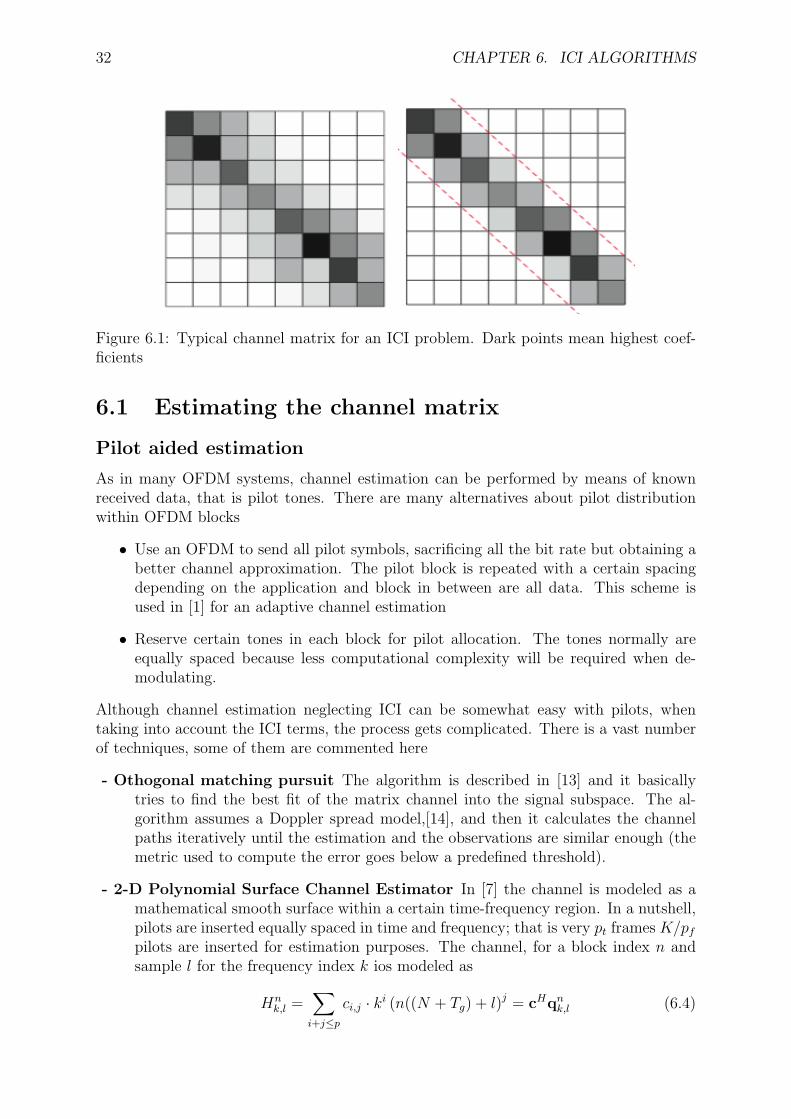
In many systems, though, the channel matrix H(n) is considered to be banded. That is,only a few adjacent subcarriers are affecting the current examined symbol like shown infigure 6.1. This specific structure is advantageous because the inverse of such matricescan be computed faster than general propertyless matrices [10]. Knowing that an OFDMsystem can have a large number of subcarriers and thus a large channel matrix, thissimplification is of great computational savings.Although the model is pretty simple, the main challenge of the algorithms is to esti-mate the channel. Several are proposed, like pilot aided channel estimation, adaptivealgorithms like a Frequency Domain Decision Feedback Equalizer (FD-DFE) or model-ing the channel variation with a Taylor approximation for example. An overview of thedemodulations techniques and their results will be explained here.

31

32 CHAPTER 6. ICI ALGORITHMS

Figure 6.1: Typical channel matrix for an ICI problem. Dark points mean highest coef-ficients

6.1 Estimating the channel matrix

Pilot aided estimation

As in many OFDM systems, channel estimation can be performed by means of knownreceived data, that is pilot tones. There are many alternatives about pilot distributionwithin OFDM blocks

• Use an OFDM to send all pilot symbols, sacrificing all the bit rate but obtaining abetter channel approximation. The pilot block is repeated with a certain spacingdepending on the application and block in between are all data. This scheme isused in [1] for an adaptive channel estimation

• Reserve certain tones in each block for pilot allocation. The tones normally areequally spaced because less computational complexity will be required when de-modulating.

Although channel estimation neglecting ICI can be somewhat easy with pilots, whentaking into account the ICI terms, the process gets complicated. There is a vast numberof techniques, some of them are commented here

- Othogonal matching pursuit The algorithm is described in [13] and it basicallytries to find the best fit of the matrix channel into the signal subspace. The al-gorithm assumes a Doppler spread model,[14], and then it calculates the channelpaths iteratively until the estimation and the observations are similar enough (themetric used to compute the error goes below a predefined threshold).

- 2-D Polynomial Surface Channel Estimator In [7] the channel is modeled as amathematical smooth surface within a certain time-frequency region. In a nutshell,pilots are inserted equally spaced in time and frequency; that is very pt frames K/pfpilots are inserted for estimation purposes. The channel, for a block index n andsample l for the frequency index k ios modeled as

Hnk,l =

∑i+j≤p

ci,j · ki (n((N + Tg) + l)j = cHqnk,l (6.4)

6.1. ESTIMATING THE CHANNEL MATRIX 33

To find the coefficients c a minimization algorithm is run using the known data.Although this estimation can be done in the frequency domain, time domain esti-mation is much more efficient because, usually, the length of the CIR is much lessthan the number of subcarriers. The previous equation then transforms into thetime domain, but the minimization process is kept similar.

- Basis Expansion Model The basic idea of this algorithm is to express each chan-nel path as a linear combination of deterministic time-varying functions definedover a limited time span. Each channel path evolution can be expressed as gl =[h0,l, · · · , hN−1,l] with N the number of samples received. The basis expansion model(BEM) express the channel as

gl = Ξηi = [ξ0, · · · , ξQ][ηl,0, · · · , ηl,Q]T (6.5)

Like the other algorithms, to find the path evolution, a minimization algorithmis run leading to an MMSE estimate for the coefficients ηi,j of the basis functionsξj for a basis of length Q. A popular choice of the basis functions is representedby complex exponentials, because they are orthonormal by definition and the finalchannel matrix H can be banded although other choices are possible.

Adaptive Frequency Channel Estimator

An effective way to estimate the channel coefficients is by means of a gradient algorithm[11]. From the a priori known symbols dk(n), an error signal is formed

Ek(n) = yk(n)−I∑

m=−I

Hk,k+m(n)dk(n) (6.6)

And P is the number of subcarriers neighbors that are considered to be interfering. Fromthis error signal, a gradient algorithm is constructed, namely LMR or RLS to iteratealong all subcarriers in the following manner:

Hk(n) = Hk−1(n) + Γ(n)εk(n) (6.7)

Defining

Hk(n) = [Hk,k−I(n), . . . , Hk,k+I ]T

εk(n) = [Ek(n)d∗k−I(n), . . . , Ek(n)d∗k+I(n)]T

Γ(n) = diag(γ−I(n), . . . , γ+I(n))

Where Γ represent the gradient coefficients and its values depend of the type of algorithmused. So, it is clear that all the K symbols should be known. This means that either wecan use pilot signals (which is not of interest) or we can make tentative decisions beforeiterating. Depending on the correctness of the a priori decisions, the channel matrix willbe accurately estimated. Simplification of this algorithm implies to restrict the numberof interfering subcarriers, being the simplest case with only two interfering neighbors(I = 1)

34 CHAPTER 6. ICI ALGORITHMS

Yk ak ×

e−jθk

+ DECISION DEVICE

bk

dk−

+pk Xk

qk

Figure 6.2: Scheme of a Frequency Domain DFE

Frequency Domain - Decision Feedback Equalizer

A decision-feedback equalizer is a nonlinear equalizer that contains a forward filter and afeedback filter. Unlike the linear equalizer, the DFE doesn’t have to estimate the explicitICI coefficients. In the classical way, the DFE was widely used for intersymbol interference(ISI) cancellation. In OFDM, information is sent among independent channels, so ICIcan be treated as ISI but in a causal and anticausal way. In ISI approaches, only symbolsthat were sent before would affect the current decision, but in the frequency domainand ICI, the influence comes from the higher and the lower subcarriers. See the schemeproposed in figure 6.2 and the corresponding explanation for more details.

Inputs of the DFE are vectors formed by 2I + 1 elements corresponding to the ICIcoefficients that must be taken into account. Normally, as in the linear equalizers, I = 1so the vectors have 3 elements. The inputs are filteres and then are multiplied by thephase corresponding to the subcarrier with index k. The output of the decision deviceis also a vector of 2I + 1 elements which come from previous decisions. A filtering ofthis output subtracted to the filtered phase-corrected input for the new input to the nextdecision module. For each iteration, the optimal coefficients conditioned to the phaseestimate are:

woptk = (E {UkU

′k})−1

E {Ukd∗k} (6.8)

wherewoptk =

[aoptk boptk

](6.9)

andUk =

[Yke

−jbθk dk

](6.10)

This process is repeated for all the subcarrier indexes and the coefficients are updatedusing RLS or LMS. Phase tracking is implemented using a second-order locked loop. Inthe system, the phase is modeled as

θk = θ0 + a2πfkT′ (6.11)

With usually θ0 = 0. From the MSE solution found for the DFE, the recursion describingthe phase tracking is done with

θk+1 = θk +G1ψk +G2

k∑i=0

ψk (6.12)

With G1 and G2 the step sizes of the loop. Normally, G2 = G1/10 and G1 is tunnedmanually observing experiment results. The gradient estimate ψk is computed as

ψk = ={pk(pk + ek)∗} (6.13)

6.1. ESTIMATING THE CHANNEL MATRIX 35

Taylor approximation

The approach used is to consider a linear channel tap variation within each OFDM block.That means that the channel has to be estimated before and after the demodulation ofthe block. The algorithm runs in the time domain, so only the CIR has to be estimated.As the CIR is related to the frequency response via a Fourier relationship, estimatingthe first is equivalent to have the latter. Going to the channel response domain can beadvantageous if we want to apply channel sparsing, hence, noise variance can be reduced.The channel estimate of the previous block is always available, so the challenge is to obtainthe next channel estimation without the use of pilots. To accomplish this, algorithm in[1] is executed and a channel esimation is calculated after making the final decisions. Wethen have the two channel estimates that can help to calculate the time variation.Let’s define the channel as a variant-time vector inside a block, from the first sample,n = 0,to the sample n = N − 1

h0 = [h0,0, h0,1, . . . , h0,L−1]T CIR in the start of the block (6.14)

hN−1 = [hN−1,0, hN−1,1, . . . , hN−1,L−1]T CIR at the end of the block (6.15)

From these two variables we can consider the CIR to vary inside a block as:

hk = h0 + k × h0 − hN−1

N − 1= h0 + k × ∆h

N − 1(6.16)

Basically, in each sample, the channel varies an amount of ∆hN−1

. So, if the received signalcan be expressed as:

Yn =L−1∑l=0

hn,ls|n−l| + nn (6.17)

Where sn is the sample n of the sent signal which is a common modulated OFDM block.Overlap add is used to convert linear convolution into circular convolution. The signalreceived is, in matrix notation:

Y = Hs + n =

h0,0 h0,N−1 . . . h0,1

h1,1 h1,0 . . . h1,2

h2,2...

. . ....

hN−1,N−1 hN−1,N−2 . . . hN−1,0

×

s0

s1...

sN−1

+ n (6.18)

The vector n contains noise. As the channel is varying, we can relate the H matrixcoefficients by the linear relationship in equation (6.18)

H =

h0,0 h0,N−1 . . . h0,1

h0,1 h0,0 . . . h0,2...

.... . .

...h0,N−1 h0,N−2 . . . h0,0

+1

N − 1diag(0, 1, 2, . . . , N−1)×

∆h0 ∆hN−1 . . . ∆h1

∆h1 ∆h0 . . . ∆h2...

.... . .

...∆hN−1 ∆hN−2 . . . ∆h0

(6.19)

To simplify notation we will express the channel as

H = A0 +1

N − 1DA1 (6.20)

From equations (6.19) and (6.20) we can see that the matrices A0 and A1 are Toeplitz.When receiving the signal, an FFT operation is performed. W will be used to denote

36 CHAPTER 6. ICI ALGORITHMS

the inverse Fourier transform so, WH denotes the Fourier transform itself. Knowing thatthe sent signal is s = Wd, the received signal becomes, in the frequency domain

y = W′HWs = W′(A0 +1

N − 1DA1)Wd + n (6.21)

The challenge is to find the Fourier transform for the matrices A0 and A1 separately tosimplify the process. As said before, it’s Toeplitz nature will define its structure

W′(A0 +1

N − 1DA1)W = (W′A0W) +

1

N − 1(W′DW)(W′A1W) (6.22)

Af0 = W′A0W (6.23)

Af1 = W′A1W (6.24)

Df = W′DW (6.25)

The received signal becomes:

y = (Af0 +

1

N − 1DfAf

1)d + n = Hd + n (6.26)

The problem resides in finding the expressions of matrices A′0, A′1 and D′. Thelatter has no difficulties since it is a fixed matrix and can be precalculated before thedemodulation process begins. As a result, D′ is a Toeplitz matrix whose first row elementsare the IFFT of the diagonal elements of D.A′0 is a little trickier to find, but after playing with the properties of A0 we can showthat it is a diagonal matrix whose elements are the Fourier transform of h0. Equivalently,A′1 is a diagonal matrix whose elements are the transform of the ∆h vector.Once found the transforms of the previous matrices and calculated the expression for Hand MMSE estimate is constructed

d = (H′H)−1H′y (6.27)

Matrix H will be typically banded, being the coefficients of the main diagonal moreimportant than the others.

6.2 Inverting the channel matrix

All along this section, several methods for estimate the channel matrix are considered.Although estimation is the most difficult part theoretically, the inversion of large matricesiand the amount of operations spent on doing so is what practical systems need to dofast. The ICI channel matrix is of dimensions K×K, quite big if an inversion is required.Since the MMSE solution of the demodulated symbols computes an inverse of this size,several approaches are possible to make it simpler.

LDLH Factorization

One of the forms of making the process faster, is to perform the inversion in two differentparts [10]. As a first step, the Channel matrix is truncated and only its main P diagonalsare only considered. As shown in equation (6.3) the solution is

d(n) = [H′(n)H(n)]−1H′(n)y(n) (6.28)

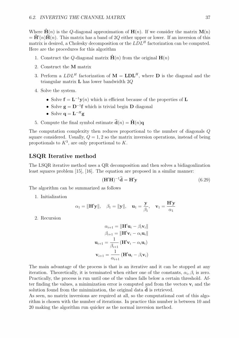
6.2. INVERTING THE CHANNEL MATRIX 37

Where H(n) is the Q-diagonal approximation of H(n). If we consider the matrix M(n)= H′(n)H(n). This matrix has a band of 2Q either upper or lower. If an inversion of thismatrix is desired, a Cholesky decomposition or the LDLH factorization can be computed.Here are the procedures for this algorithm

1. Construct the Q-diagonal matrix H(n) from the original H(n)

2. Construct the M matrix

3. Perform a LDLH factorization of M = LDLH , where D is the diagonal and thetriangular matrix L has lower bandwidth 2Q

4. Solve the system.

• Solve f = L−1y(n) which is efficient because of the properties of L

• Solve g = D−1f which is trivial begin D diagonal

• Solve q = L−Hg

5. Compute the final symbol estimate d(n) = H(n)q

The computation complexity then reduces proportional to the number of diagonals Qsquare considered. Usually, Q = 1, 2 so the matrix inversion operations, instead of beingpropotionals to K3, are only proportional to K.

LSQR Iterative method

The LSQR iterative method uses a QR decomposition and then solves a bidiagonlizationleast squares problem [15], [16]. The equation are proposed in a similar manner:

(H′H)−1d = H′y (6.29)

The algorithm can be summarized as follows

1. Initialization

α1 = ‖H′y‖, β1 = ‖y‖, u1 =y

β1

, v1 =H′y

α1

2. Recursion

αi+1 = ‖H′ui − βivi‖βi+1 = ‖H′vi − αiui‖

ui+1 =1

βi+1

(H′vi − αiui)

vi+1 =1

αi+1

(H′ui − βivi)

The main advantage of the process is that is an iterative and it can be stopped at anyiteration. Theoretically, it is terminated when either one of the constants, αi, βi is zero.Practically, the process is run until one of the values falls below a certain threshold. Af-ter finding the values, a minimization error is computed and from the vectors vi and thesolution found from the minimization, the original data d is retrieved.As seen, no matrix inversions are required at all, so the computational cost of this algo-rithm is chosen with the number of iterations. In practice this number is between 10 and20 making the algorithm run quicker as the normal inversion method.

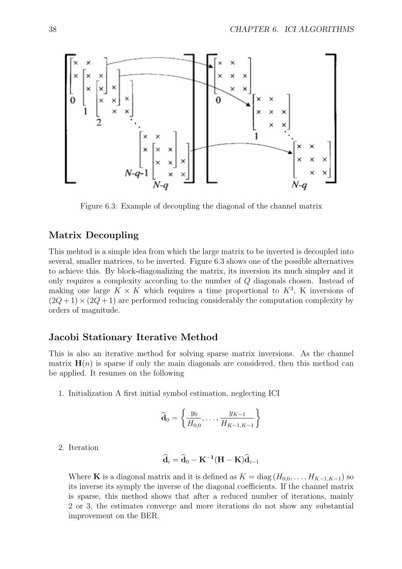
38 CHAPTER 6. ICI ALGORITHMS

Figure 6.3: Example of decoupling the diagonal of the channel matrix

Matrix Decoupling

This mehtod is a simple idea from which the large matrix to be inverted is decoupled intoseveral, smaller matrices, to be inverted. Figure 6.3 shows one of the possible alternativesto achieve this. By block-diagonalizing the matrix, its inversion its much simpler and itonly requires a complexity according to the number of Q diagonals chosen. Instead ofmaking one large K × K which requires a time proportional to K3, K inversions of(2Q+ 1)× (2Q+ 1) are performed reducing considerably the computation complexity byorders of magnitude.

Jacobi Stationary Iterative Method

This is also an iterative method for solving sparse matrix inversions. As the channelmatrix H(n) is sparse if only the main diagonals are considered, then this method canbe applied. It resumes on the following

1. Initialization A first initial symbol estimation, neglecting ICI

d0 =

{y0

H0,0

, . . . ,yK−1

HK−1,K−1

}

2. Iteration

di = d0 −K−1(H−K)di−1

Where K is a diagonal matrix and it is defined as K = diag (H0,0, . . . , HK−1,K−1) soits inverse its symply the inverse of the diagonal coefficients. If the channel matrixis sparse, this method shows that after a reduced number of iterations, mainly2 or 3, the estimates converge and more iterations do not show any substantialimprovement on the BER.

6.2. INVERTING THE CHANNEL MATRIX 39

Matrix Simplification

This technique was tried with algorithm in [12]. The point is to observe that the ICIcoefficients of the adjacent subcarriers can be, in typical cases, 10dB in amplitude belowthe corresponding coefficient. That is HdB

k,k±1 + 10dB = HdBk,k . Assuming this result, to

compute the LS estimate, the following approximation can be done:

(H′(n)H(n)

)−1

≈ diag

(1∑K−1

k=0 ‖H0,k‖2, . . . ,

1∑K−1k=0 ‖HK−1,k‖2

)(6.30)

Which is simply a truncation of the multiplication of the left hand side of the equation.Empirical results show that a difference of 30dB is usually found between the main andthe upper diagonal, so truncation can be performed without observing any degradationon BER. Therefore, the final solution is

d(n) = diag

(1∑K−1

k=0 ‖H0,k‖2, . . . ,

1∑K−1k=0 ‖HK−1,k‖2

)H′(n)y(n) (6.31)

Which doeas not require any matrix inversion.

Part III

Results and Conclusions

41

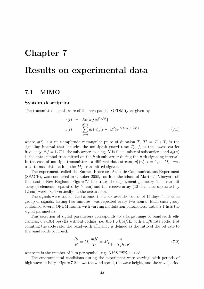
Chapter 7

Results on experimental data

7.1 MIMO

System description

The transmitted signals were of the zero-padded OFDM type, given by

s(t) = Re{u(t)ej2πf0t}

u(t) =K−1∑k=0

dk(n)g(t− nT ′)ej2πk∆f(t−nT ′) (7.1)

where g(t) is a unit-amplitude rectangular pulse of duration T , T ′ = T + Tg is thesignaling interval that includes the multipath guard time Tg, f0 is the lowest carrierfrequency, ∆f = 1/T is the subcarrier spacing, K is the number of subcarriers, and dk(n)is the data sumbol transmitted on the k-th subcarrier during the n-th signaling interval.In the case of multiple transmitters, a different data stream, dtk(n), t = 1, . . .MT , wasused to modulate each of the MT transmitted signals.

The experiment, called the Surface Processes Acoustic Communications Experiment(SPACE), was conducted in October 2008, south of the island of Martha’s Vineyard offthe coast of New England. Figure 7.1 illustrates the deployment geometry. The transmitarray (4 elements separated by 50 cm) and the receive array (12 elements, separated by12 cm) were fixed vertically on the ocean floor.

The signals were transmitted around the clock over the course of 15 days. The samegroup of signals, lasting two minutes, was repeated every two hours. Each such groupcontained several OFDM frames with varying modulation parameters. Table 7.1 lists thesignal parameters.

This selection of signal parameters corresponds to a large range of bandwidth effi-ciencies, 0.9-10.4 bps/Hz without coding, i.e. 0.1-1.6 bps/Hz with a 1/6 rate code. Notcounting the code rate, the bandwidth efficiency is defined as the ratio of the bit rate tothe bandwidth occupied,

Rb

B= MT

mK

T ′= MT

m

1 + TgB/K(7.2)

where m is the number of bits per symbol, e.g. 3 if 8-PSK is used.The environmental conditions during the experiment were varying, with periods of

high wave activity. Figure 7.2 shows the wind speed, the wave height, and the wave period

43

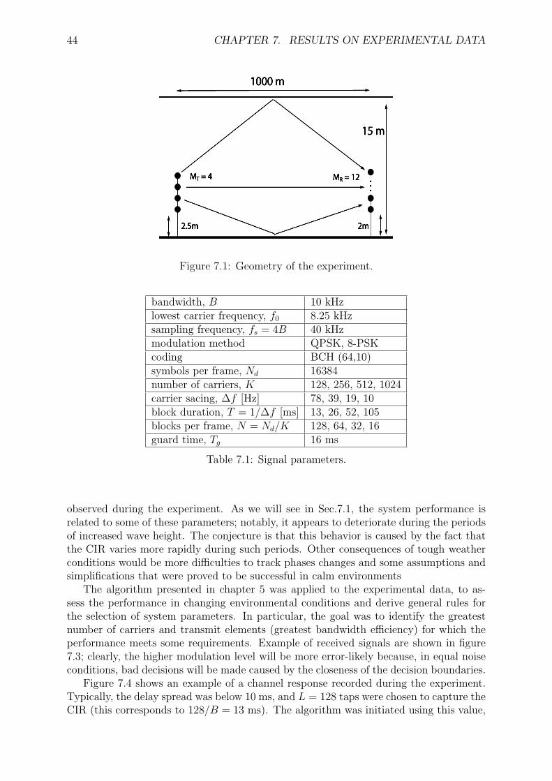
44 CHAPTER 7. RESULTS ON EXPERIMENTAL DATA

Figure 7.1: Geometry of the experiment.

bandwidth, B 10 kHzlowest carrier frequency, f0 8.25 kHzsampling frequency, fs = 4B 40 kHzmodulation method QPSK, 8-PSKcoding BCH (64,10)symbols per frame, Nd 16384number of carriers, K 128, 256, 512, 1024carrier sacing, ∆f [Hz] 78, 39, 19, 10block duration, T = 1/∆f [ms] 13, 26, 52, 105blocks per frame, N = Nd/K 128, 64, 32, 16guard time, Tg 16 ms

Table 7.1: Signal parameters.

observed during the experiment. As we will see in Sec.7.1, the system performance isrelated to some of these parameters; notably, it appears to deteriorate during the periodsof increased wave height. The conjecture is that this behavior is caused by the fact thatthe CIR varies more rapidly during such periods. Other consequences of tough weatherconditions would be more difficulties to track phases changes and some assumptions andsimplifications that were proved to be successful in calm environments

The algorithm presented in chapter 5 was applied to the experimental data, to as-sess the performance in changing environmental conditions and derive general rules forthe selection of system parameters. In particular, the goal was to identify the greatestnumber of carriers and transmit elements (greatest bandwidth efficiency) for which theperformance meets some requirements. Example of received signals are shown in figure7.3; clearly, the higher modulation level will be more error-likely because, in equal noiseconditions, bad decisions will be made caused by the closeness of the decision boundaries.

Figure 7.4 shows an example of a channel response recorded during the experiment.Typically, the delay spread was below 10 ms, and L = 128 taps were chosen to capture theCIR (this corresponds to 128/B = 13 ms). The algorithm was initiated using this value,

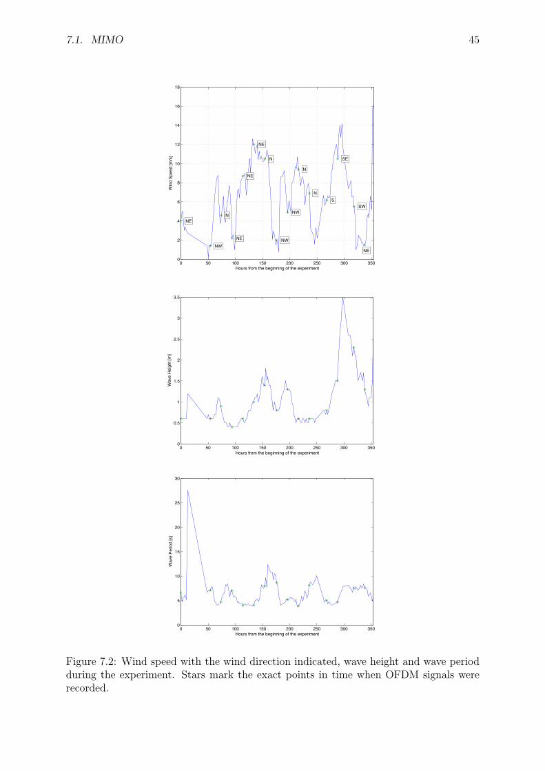
7.1. MIMO 45

0 50 100 150 200 250 300 3500

2

4

6

8

10

12

14

16

18

Hours from the beginning of the experiment

NE

NW

N

NE

NE

NE

N

NW

NW

N

NS

SE

SW

NE

Win

d Sp

eed

[m/s

]

0 50 100 150 200 250 300 3500

0.5

1

1.5

2

2.5

3

3.5

Hours from the beginning of the experiment

Wav

e He

ight

[m]

0 50 100 150 200 250 300 3500

5

10

15

20

25

30

Hours from the beginning of the experiment

Wav

e Pe

riod

[s]

Figure 7.2: Wind speed with the wind direction indicated, wave height and wave periodduring the experiment. Stars mark the exact points in time when OFDM signals wererecorded.

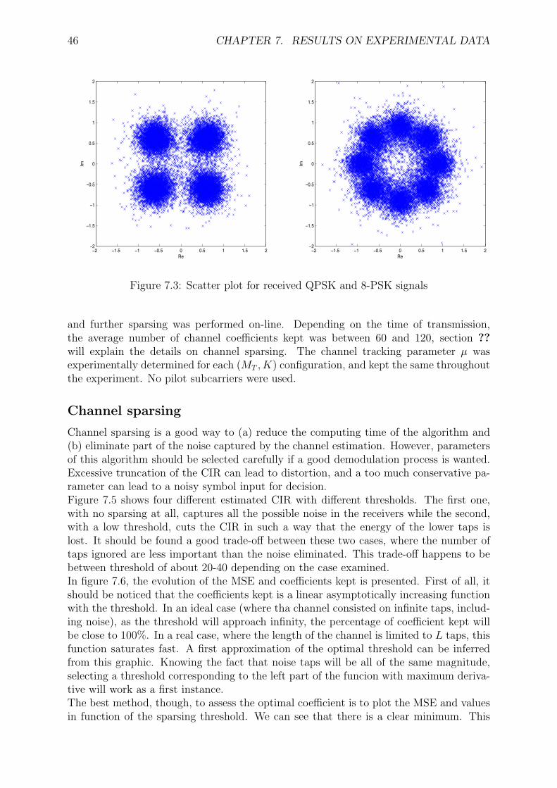
46 CHAPTER 7. RESULTS ON EXPERIMENTAL DATA

−2 −1.5 −1 −0.5 0 0.5 1 1.5 2−2

−1.5

−1

−0.5

0

0.5

1

1.5

2

Re

Im

−2 −1.5 −1 −0.5 0 0.5 1 1.5 2−2

−1.5

−1

−0.5

0

0.5

1

1.5

2

Re

Im

Figure 7.3: Scatter plot for received QPSK and 8-PSK signals

and further sparsing was performed on-line. Depending on the time of transmission,the average number of channel coefficients kept was between 60 and 120, section ??will explain the details on channel sparsing. The channel tracking parameter µ wasexperimentally determined for each (MT , K) configuration, and kept the same throughoutthe experiment. No pilot subcarriers were used.

Channel sparsing

Channel sparsing is a good way to (a) reduce the computing time of the algorithm and(b) eliminate part of the noise captured by the channel estimation. However, parametersof this algorithm should be selected carefully if a good demodulation process is wanted.Excessive truncation of the CIR can lead to distortion, and a too much conservative pa-rameter can lead to a noisy symbol input for decision.Figure 7.5 shows four different estimated CIR with different thresholds. The first one,with no sparsing at all, captures all the possible noise in the receivers while the second,with a low threshold, cuts the CIR in such a way that the energy of the lower taps islost. It should be found a good trade-off between these two cases, where the number oftaps ignored are less important than the noise eliminated. This trade-off happens to bebetween threshold of about 20-40 depending on the case examined.In figure 7.6, the evolution of the MSE and coefficients kept is presented. First of all, itshould be noticed that the coefficients kept is a linear asymptotically increasing functionwith the threshold. In an ideal case (where tha channel consisted on infinite taps, includ-ing noise), as the threshold will approach infinity, the percentage of coefficient kept willbe close to 100%. In a real case, where the length of the channel is limited to L taps, thisfunction saturates fast. A first approximation of the optimal threshold can be inferredfrom this graphic. Knowing the fact that noise taps will be all of the same magnitude,selecting a threshold corresponding to the left part of the funcion with maximum deriva-tive will work as a first instance.The best method, though, to assess the optimal coefficient is to plot the MSE and valuesin function of the sparsing threshold. We can see that there is a clear minimum. This

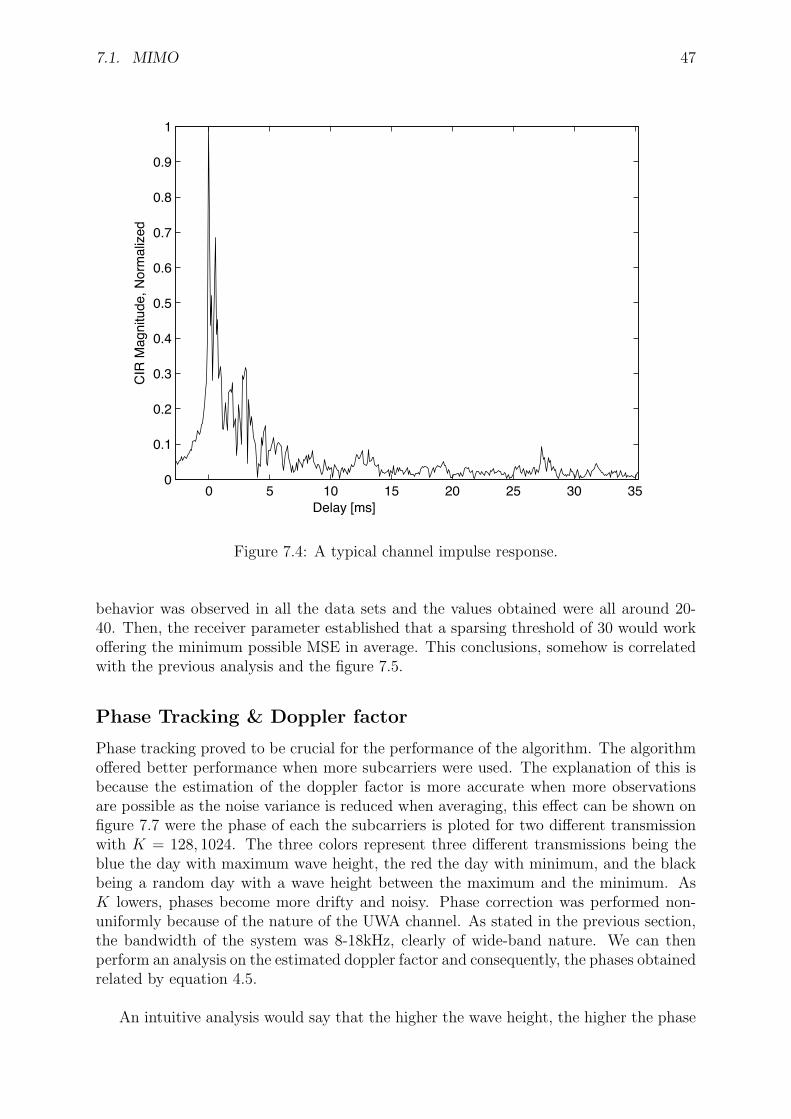
7.1. MIMO 47

0 5 10 15 20 25 30 350

0.1

0.2

0.3

0.4

0.5

0.6

0.7

0.8

0.9

1

Delay [ms]

CIR

Mag

nitu

de, N

orm

alize

d

Figure 7.4: A typical channel impulse response.

behavior was observed in all the data sets and the values obtained were all around 20-40. Then, the receiver parameter established that a sparsing threshold of 30 would workoffering the minimum possible MSE in average. This conclusions, somehow is correlatedwith the previous analysis and the figure 7.5.

Phase Tracking & Doppler factor

Phase tracking proved to be crucial for the performance of the algorithm. The algorithmoffered better performance when more subcarriers were used. The explanation of this isbecause the estimation of the doppler factor is more accurate when more observationsare possible as the noise variance is reduced when averaging, this effect can be shown onfigure 7.7 were the phase of each the subcarriers is ploted for two different transmissionwith K = 128, 1024. The three colors represent three different transmissions being theblue the day with maximum wave height, the red the day with minimum, and the blackbeing a random day with a wave height between the maximum and the minimum. AsK lowers, phases become more drifty and noisy. Phase correction was performed non-uniformly because of the nature of the UWA channel. As stated in the previous section,the bandwidth of the system was 8-18kHz, clearly of wide-band nature. We can thenperform an analysis on the estimated doppler factor and consequently, the phases obtainedrelated by equation 4.5.

An intuitive analysis would say that the higher the wave height, the higher the phase

48 CHAPTER 7. RESULTS ON EXPERIMENTAL DATA

−5 0 5 10 15 20 25 300

0.1

0.2

0.3

0.4

0.5

0.6

0.7

0.8

0.9

1Channel for Transmitter 1

Time [ms]−5 0 5 10 15 20 25 30

0

0.1

0.2

0.3

0.4

0.5

0.6

0.7

0.8

0.9

1Channel for Transmitter 1

Time [ms]

−5 0 5 10 15 20 25 300

0.1

0.2

0.3

0.4

0.5

0.6

0.7

0.8

0.9

1Channel for Transmitter 1

Time [ms]−5 0 5 10 15 20 25 30

0

0.1

0.2

0.3

0.4

0.5

0.6

0.7

0.8

0.9

1Channel for Transmitter 1

Time [ms]

Figure 7.5: Channel Impulse Response estimated for a different number of threshold.From left to right and top to bottom: no sparsing, 10, 30, 60.

0 20 40 60 80 100 120 140 160 180 200−6.4

−6.3

−6.2

−6.1

−6

−5.9

−5.8

−5.7

−5.6

−5.5

−5.4

Sparsing Threshold

MS

E [

dB

]

0 20 40 60 80 100 120 140 160 180 2000

10

20

30

40

50

60

70

80

90

100

Sparsing Threshold

Co

eff

icie

nts

Ke

pt

(%)

Figure 7.6: MSE and Coefficients kept (left to right) for a different number of sparsingthresholds

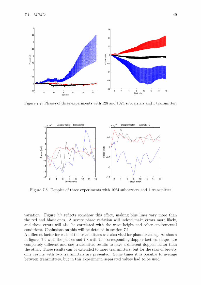
7.1. MIMO 49

0 20 40 60 80 100 120!0.5

0

0.5

1

1.5

2

2.5

3

3.5

4

Block Index

Ph

ase

[ra

d]

2 4 6 8 10 12 14 16−0.8

−0.6

−0.4

−0.2

0

0.2

0.4

0.6

Block Index

Phase

[ra

d]

Figure 7.7: Phases of three experiments with 128 and 1024 subcarriers and 1 transmitter.

2 4 6 8 10 12 14 16−8

−6

−4

−2

0

2

4

6

8

10x 10−6 Doppler factor − Transmitter 1

Block Index

Pha

se [r

ad]

2 4 6 8 10 12 14 16−1.5

−1

−0.5

0

0.5

1x 10−5 Doppler factor − Transmitter 2

Block Index

Pha

se [r

ad]

Figure 7.8: Doppler of three experiments with 1024 subcarriers and 1 transmitter

variation. Figure 7.7 reflects somehow this effect, making blue lines vary more thanthe red and black ones. A severe phase variation will indeed make errors more likely,and these errors will also be correlated with the wave height and other enviromentalconditions. Conlusions on this will be detailed in section 7.1A different factor for each of the transmitters was also vital for phase tracking. As shownin figures 7.9 with the phases and 7.8 with the corresponding doppler factors, shapes arecompletely different and one transmitter results to have a different doppler factor thanthe other. These results can be extended to more transmitters, but for the sake of brevityonly results with two transmitters are presented. Some times it is possible to averagebetween transmitters, but in this experiment, separated values had to be used.

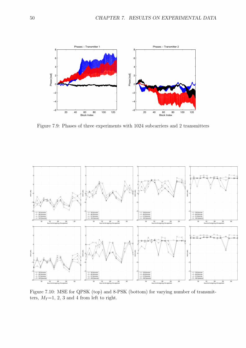
50 CHAPTER 7. RESULTS ON EXPERIMENTAL DATA

20 40 60 80 100 120−6

−4

−2

0

2

4

6

8Phases − Transmitter 1

Block Index

Phas

e [ra

d]

20 40 60 80 100 120−6

−4

−2

0

2

4

6

8Phases − Transmitter 2

Block Index

Phas

e [ra

d]Figure 7.9: Phases of three experiments with 1024 subcarriers and 2 transmitters

100 150 200 250 300−20

−15

−10

−5

0

5

10

Hours from the beginning of the experiment

MS

E [

dB

]

128 Subcarriers256 Subcarriers512 Subcarriers1024 Subcarriers

100 150 200 250 300−20

−15

−10

−5

0

5

10

Hours from the beginning of the experiment

MS

E [

dB

]

128 Subcarriers256 Subcarriers512 Subcarriers1024 Subcarriers

100 150 200 250 300−20

−15

−10

−5

0

5

10

Hours from the beginning of the experiment

MS

E [

dB

]

128 Subcarriers256 Subcarriers512 Subcarriers1024 Subcarriers

100 150 200 250 300−20

−15

−10

−5

0

5

10

Hours from the beginning of the experiment

MS

E [

dB

]

128 Subcarriers256 Subcarriers512 Subcarriers1024 Subcarriers

100 150 200 250 300−20

−15

−10

−5

0

5

10

Hours from the beginning of the experiment

MS

E [

dB

]

128 Subcarriers256 Subcarriers512 Subcarriers1024 Subcarriers

100 150 200 250 300−20

−15

−10

−5

0

5

10

Hours from the beginning of the experiment

MS

E [

dB

]

128 Subcarriers256 Subcarriers512 Subcarriers1024 Subcarriers

100 150 200 250 300−20

−15

−10

−5

0

5

10

Hours from the beginning of the experiment

MS

E [

dB

]

128 Subcarriers256 Subcarriers512 Subcarriers1024 Subcarriers

100 150 200 250 300−20

−15

−10

−5

0

5

10

Hours from the beginning of the experiment

MS

E [

dB

]

128 Subcarriers256 Subcarriers512 Subcarriers1024 Subcarriers

Figure 7.10: MSE for QPSK (top) and 8-PSK (bottom) for varying number of transmit-ters, MT=1, 2, 3 and 4 from left to right.

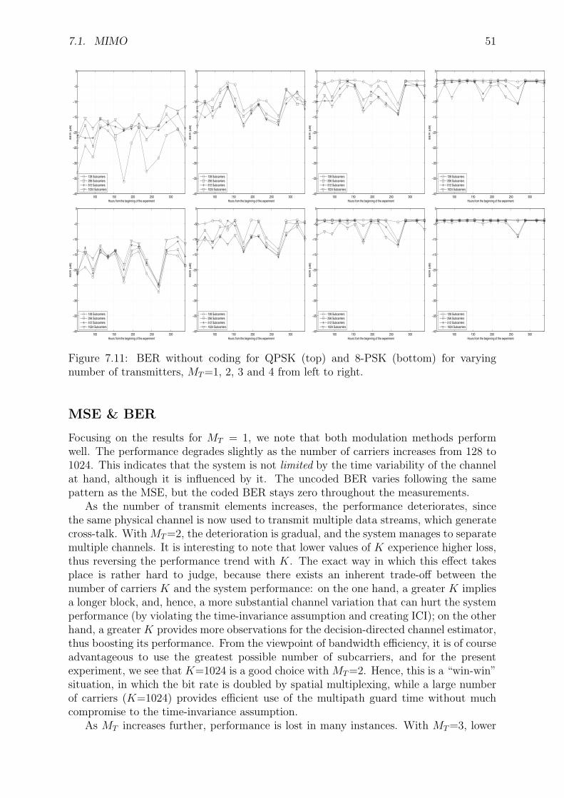
7.1. MIMO 51

100 150 200 250 300−40

−35

−30

−25

−20

−15

−10

−5

0

Hours from the beginning of the experiment

BE

R [

dB

]

128 Subcarriers256 Subcarriers512 Subcarriers1024 Subcarriers

100 150 200 250 300−40

−35

−30

−25

−20

−15

−10

−5

0

Hours from the beginning of the experiment

BE

R [

dB

]

128 Subcarriers256 Subcarriers512 Subcarriers1024 Subcarriers

100 150 200 250 300−40

−35

−30

−25

−20

−15

−10

−5

0

Hours from the beginning of the experiment

BE

R [

dB

]

128 Subcarriers256 Subcarriers512 Subcarriers1024 Subcarriers

100 150 200 250 300−40

−35

−30

−25

−20

−15

−10

−5

0

Hours from the beginning of the experiment

BE

R [

dB

]

128 Subcarriers256 Subcarriers512 Subcarriers1024 Subcarriers

100 150 200 250 300−40

−35

−30

−25

−20

−15

−10

−5

0

Hours from the beginning of the experiment

BE

R [

dB

]

128 Subcarriers256 Subcarriers512 Subcarriers1024 Subcarriers

100 150 200 250 300−40

−35

−30

−25

−20

−15

−10

−5

0

Hours from the beginning of the experiment

BE

R [

dB

]

128 Subcarriers256 Subcarriers512 Subcarriers1024 Subcarriers

100 150 200 250 300−40

−35

−30

−25

−20

−15

−10

−5

0

Hours from the beginning of the experiment

BE

R [

dB

]

128 Subcarriers256 Subcarriers512 Subcarriers1024 Subcarriers

100 150 200 250 300−40

−35

−30

−25

−20

−15

−10

−5

0

Hours from the beginning of the experiment

BE

R [

dB

]

128 Subcarriers256 Subcarriers512 Subcarriers1024 Subcarriers

Figure 7.11: BER without coding for QPSK (top) and 8-PSK (bottom) for varyingnumber of transmitters, MT=1, 2, 3 and 4 from left to right.

MSE & BER

Focusing on the results for MT = 1, we note that both modulation methods performwell. The performance degrades slightly as the number of carriers increases from 128 to1024. This indicates that the system is not limited by the time variability of the channelat hand, although it is influenced by it. The uncoded BER varies following the samepattern as the MSE, but the coded BER stays zero throughout the measurements.

As the number of transmit elements increases, the performance deteriorates, sincethe same physical channel is now used to transmit multiple data streams, which generatecross-talk. With MT=2, the deterioration is gradual, and the system manages to separatemultiple channels. It is interesting to note that lower values of K experience higher loss,thus reversing the performance trend with K. The exact way in which this effect takesplace is rather hard to judge, because there exists an inherent trade-off between thenumber of carriers K and the system performance: on the one hand, a greater K impliesa longer block, and, hence, a more substantial channel variation that can hurt the systemperformance (by violating the time-invariance assumption and creating ICI); on the otherhand, a greater K provides more observations for the decision-directed channel estimator,thus boosting its performance. From the viewpoint of bandwidth efficiency, it is of courseadvantageous to use the greatest possible number of subcarriers, and for the presentexperiment, we see that K=1024 is a good choice with MT=2. Hence, this is a “win-win”situation, in which the bit rate is doubled by spatial multiplexing, while a large numberof carriers (K=1024) provides efficient use of the multipath guard time without muchcompromise to the time-invariance assumption.

As MT increases further, performance is lost in many instances. With MT=3, lower

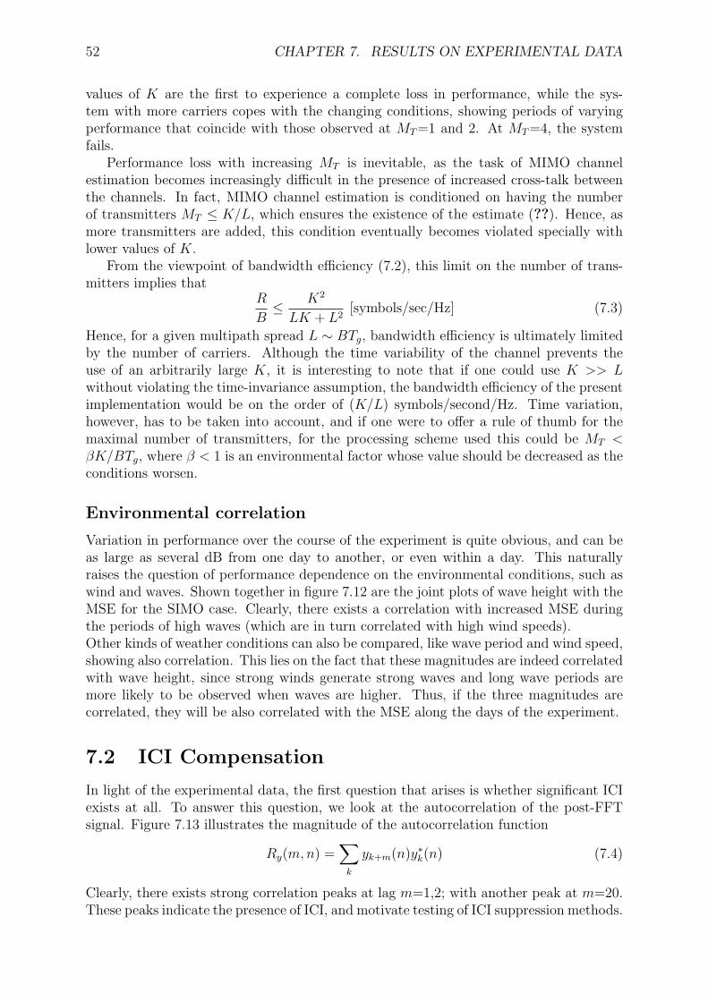
52 CHAPTER 7. RESULTS ON EXPERIMENTAL DATA

values of K are the first to experience a complete loss in performance, while the sys-tem with more carriers copes with the changing conditions, showing periods of varyingperformance that coincide with those observed at MT=1 and 2. At MT=4, the systemfails.

Performance loss with increasing MT is inevitable, as the task of MIMO channelestimation becomes increasingly difficult in the presence of increased cross-talk betweenthe channels. In fact, MIMO channel estimation is conditioned on having the numberof transmitters MT ≤ K/L, which ensures the existence of the estimate (??). Hence, asmore transmitters are added, this condition eventually becomes violated specially withlower values of K.

From the viewpoint of bandwidth efficiency (7.2), this limit on the number of trans-mitters implies that

R

B≤ K2

LK + L2[symbols/sec/Hz] (7.3)

Hence, for a given multipath spread L ∼ BTg, bandwidth efficiency is ultimately limitedby the number of carriers. Although the time variability of the channel prevents theuse of an arbitrarily large K, it is interesting to note that if one could use K >> Lwithout violating the time-invariance assumption, the bandwidth efficiency of the presentimplementation would be on the order of (K/L) symbols/second/Hz. Time variation,however, has to be taken into account, and if one were to offer a rule of thumb for themaximal number of transmitters, for the processing scheme used this could be MT <βK/BTg, where β < 1 is an environmental factor whose value should be decreased as theconditions worsen.

Environmental correlation

Variation in performance over the course of the experiment is quite obvious, and can beas large as several dB from one day to another, or even within a day. This naturallyraises the question of performance dependence on the environmental conditions, such aswind and waves. Shown together in figure 7.12 are the joint plots of wave height with theMSE for the SIMO case. Clearly, there exists a correlation with increased MSE duringthe periods of high waves (which are in turn correlated with high wind speeds).Other kinds of weather conditions can also be compared, like wave period and wind speed,showing also correlation. This lies on the fact that these magnitudes are indeed correlatedwith wave height, since strong winds generate strong waves and long wave periods aremore likely to be observed when waves are higher. Thus, if the three magnitudes arecorrelated, they will be also correlated with the MSE along the days of the experiment.

7.2 ICI Compensation

In light of the experimental data, the first question that arises is whether significant ICIexists at all. To answer this question, we look at the autocorrelation of the post-FFTsignal. Figure 7.13 illustrates the magnitude of the autocorrelation function

Ry(m,n) =∑k

yk+m(n)y∗k(n) (7.4)

Clearly, there exists strong correlation peaks at lag m=1,2; with another peak at m=20.These peaks indicate the presence of ICI, and motivate testing of ICI suppression methods.

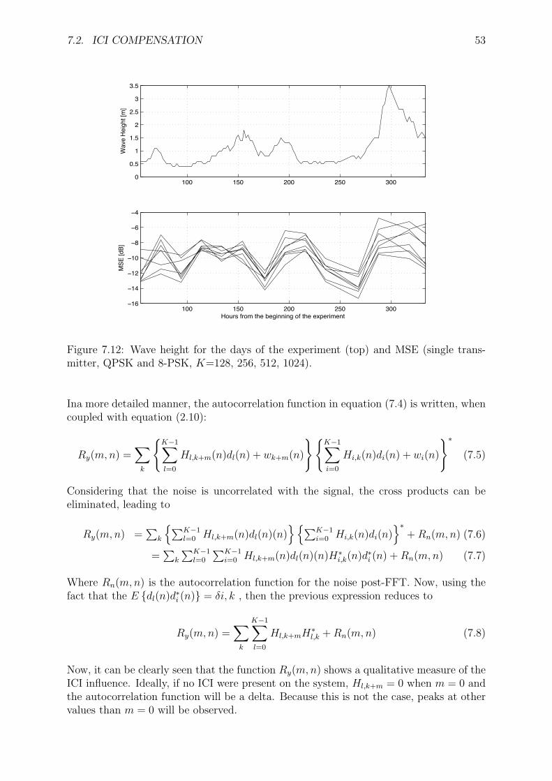
7.2. ICI COMPENSATION 53

100 150 200 250 3000

0.5

1

1.5

2

2.5

3

3.5

Wav

e He

ight

[m]

100 150 200 250 300−16

−14

−12

−10

−8

−6

−4

Hours from the beginning of the experiment

MSE

[dB]

Figure 7.12: Wave height for the days of the experiment (top) and MSE (single trans-mitter, QPSK and 8-PSK, K=128, 256, 512, 1024).

Ina more detailed manner, the autocorrelation function in equation (7.4) is written, whencoupled with equation (2.10):

Ry(m,n) =∑k

{K−1∑l=0

Hl,k+m(n)dl(n) + wk+m(n)

}{K−1∑i=0

Hi,k(n)di(n) + wi(n)

}∗(7.5)

Considering that the noise is uncorrelated with the signal, the cross products can beeliminated, leading to

Ry(m,n) =∑

k

{∑K−1l=0 Hl,k+m(n)dl(n)(n)

}{∑K−1i=0 Hi,k(n)di(n)

}∗+Rn(m,n) (7.6)

=∑

k

∑K−1l=0

∑K−1i=0 Hl,k+m(n)dl(n)(n)H∗i,k(n)d∗i (n) +Rn(m,n) (7.7)

Where Rn(m,n) is the autocorrelation function for the noise post-FFT. Now, using thefact that the E {dl(n)d∗i (n)} = δi, k , then the previous expression reduces to

Ry(m,n) =∑k

K−1∑l=0

Hl,k+mH∗l,k +Rn(m,n) (7.8)

Now, it can be clearly seen that the function Ry(m,n) shows a qualitative measure of theICI influence. Ideally, if no ICI were present on the system, Hl,k+m = 0 when m = 0 andthe autocorrelation function will be a delta. Because this is not the case, peaks at othervalues than m = 0 will be observed.

54 CHAPTER 7. RESULTS ON EXPERIMENTAL DATA

−10 −5 0 5 10

−18

−16

−14

−12

−10

−8

−6

−4

−2

0

Subcarrier Difference

Cro

ss C

orre

latio

n [d

B]

Figure 7.13: Autocorrlation of a received signal (QPSK, K = 1024) after FFT demodu-lation.

Taylor approximation

Figure 7.14 illustrates the performance of this algorithm on an experimental data set.After estimating the channel, a linear equalizer is built using a varying number I of ICIcoefficients, as before. The performance of this scheme is very good with a single ICI co-efficient, yielding a 1-5 dB improvement at very low computational complexity and littleoverhead (only the first block is used for training and no pilots after that were used).Other I were tried, leading to similar performance. Obviously I has to be kept as small aspossible because of computational expenses. Furthermore, keeping I low eliminates thenoise variance which is also contained in the estimated channel matrix. Like in channelsparsing, if the power of the noise is known, the coefficients could be cut off at a certainthreshold.It is important to notice, that this design, although very simple, lead to good improve-ments. Hence, this result demonstrates that a careful receiver design, which respects theunderlying physical processes, can be used to significantly improve the performance, thuspushing the limits on the data rate supported by the band-limited acoustic channel.

Compensation on SIMO systems

In a multichannel receiver, an ICI equalizer is associated with each receiving element. Theequalizer corresponding to the r-th receiving element utilizes channel coefficients Hr

k,l(n),

resulting in a set of (preliminary) data symbol estimates, drk(n), one for each receivingelement r = 1, . . .MR life shown in figure 7.15. The data estimates are obtained using

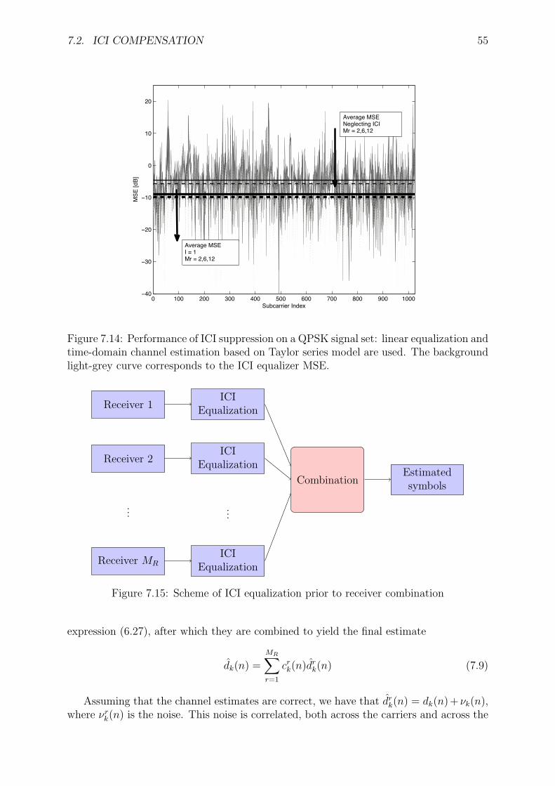
7.2. ICI COMPENSATION 55

0 100 200 300 400 500 600 700 800 900 1000−40

−30

−20

−10

0

10

20

Subcarrier Index

MSE

[dB]

Average MSENeglecting ICIMr = 2,6,12

Average MSEI = 1Mr = 2,6,12

Figure 7.14: Performance of ICI suppression on a QPSK signal set: linear equalization andtime-domain channel estimation based on Taylor series model are used. The backgroundlight-grey curve corresponds to the ICI equalizer MSE.

Receiver 1

Receiver 2

...

Receiver MR

ICIEqualization

ICIEqualization

...

ICIEqualization

CombinationEstimatedsymbols

Figure 7.15: Scheme of ICI equalization prior to receiver combination

expression (6.27), after which they are combined to yield the final estimate

dk(n) =

MR∑r=1

crk(n)drk(n) (7.9)

Assuming that the channel estimates are correct, we have that drk(n) = dk(n) + νk(n),where νrk(n) is the noise. This noise is correlated, both across the carriers and across the

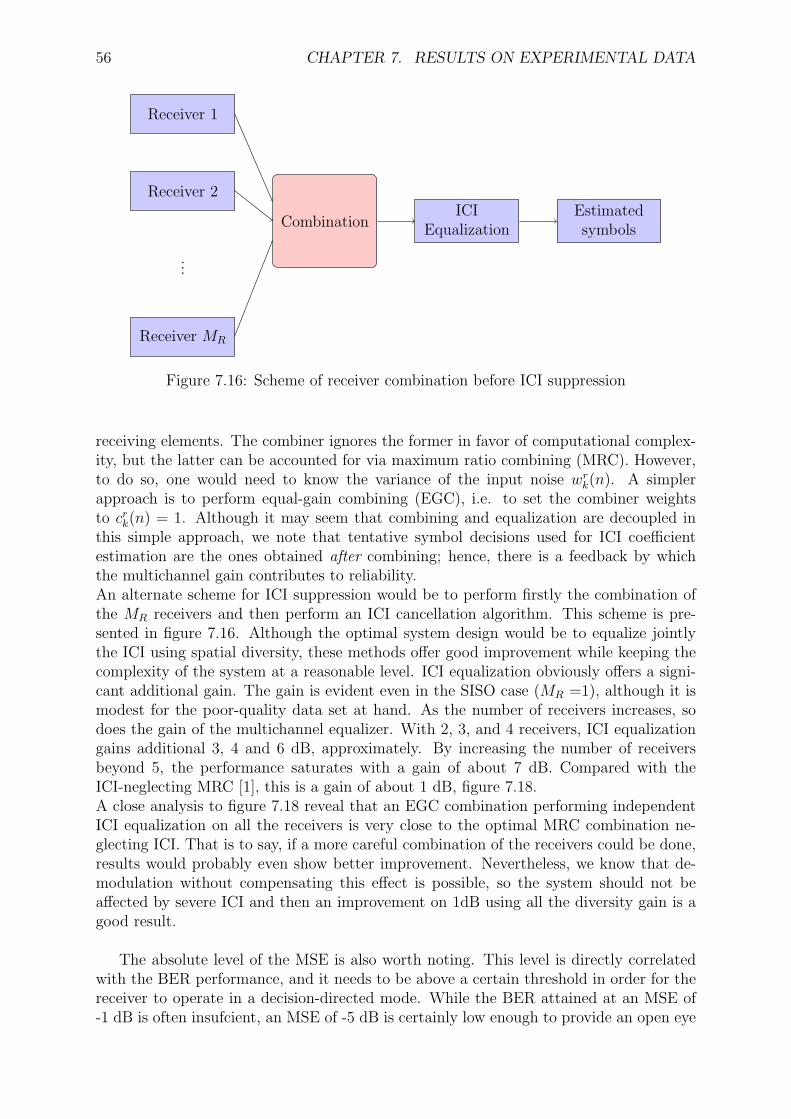
56 CHAPTER 7. RESULTS ON EXPERIMENTAL DATA

Receiver 1

Receiver 2

...

Receiver MR

CombinationICI

EqualizationEstimatedsymbols

Figure 7.16: Scheme of receiver combination before ICI suppression

receiving elements. The combiner ignores the former in favor of computational complex-ity, but the latter can be accounted for via maximum ratio combining (MRC). However,to do so, one would need to know the variance of the input noise wrk(n). A simplerapproach is to perform equal-gain combining (EGC), i.e. to set the combiner weightsto crk(n) = 1. Although it may seem that combining and equalization are decoupled inthis simple approach, we note that tentative symbol decisions used for ICI coefficientestimation are the ones obtained after combining; hence, there is a feedback by whichthe multichannel gain contributes to reliability.An alternate scheme for ICI suppression would be to perform firstly the combination ofthe MR receivers and then perform an ICI cancellation algorithm. This scheme is pre-sented in figure 7.16. Although the optimal system design would be to equalize jointlythe ICI using spatial diversity, these methods offer good improvement while keeping thecomplexity of the system at a reasonable level. ICI equalization obviously offers a signi-cant additional gain. The gain is evident even in the SISO case (MR =1), although it ismodest for the poor-quality data set at hand. As the number of receivers increases, sodoes the gain of the multichannel equalizer. With 2, 3, and 4 receivers, ICI equalizationgains additional 3, 4 and 6 dB, approximately. By increasing the number of receiversbeyond 5, the performance saturates with a gain of about 7 dB. Compared with theICI-neglecting MRC [1], this is a gain of about 1 dB, figure 7.18.A close analysis to figure 7.18 reveal that an EGC combination performing independentICI equalization on all the receivers is very close to the optimal MRC combination ne-glecting ICI. That is to say, if a more careful combination of the receivers could be done,results would probably even show better improvement. Nevertheless, we know that de-modulation without compensating this effect is possible, so the system should not beaffected by severe ICI and then an improvement on 1dB using all the diversity gain is agood result.

The absolute level of the MSE is also worth noting. This level is directly correlatedwith the BER performance, and it needs to be above a certain threshold in order for thereceiver to operate in a decision-directed mode. While the BER attained at an MSE of-1 dB is often insufcient, an MSE of -5 dB is certainly low enough to provide an open eye

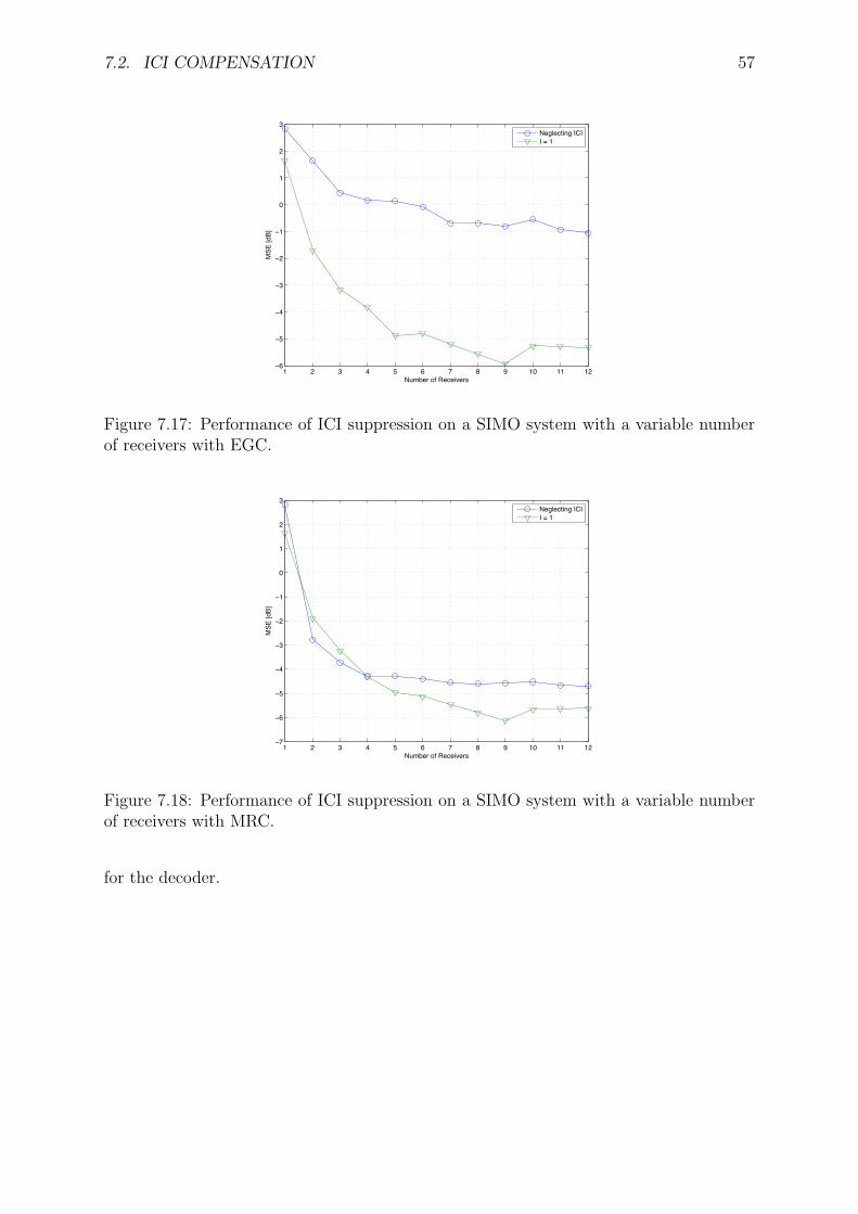
7.2. ICI COMPENSATION 57

1 2 3 4 5 6 7 8 9 10 11 12−6

−5

−4

−3

−2

−1

0

1

2

3

Number of Receivers

MSE

[dB]

Neglecting ICII = 1

Figure 7.17: Performance of ICI suppression on a SIMO system with a variable numberof receivers with EGC.

1 2 3 4 5 6 7 8 9 10 11 12−7

−6

−5

−4

−3

−2

−1

0

1

2

3

Number of Receivers

MSE

[dB]

Neglecting ICII = 1

Figure 7.18: Performance of ICI suppression on a SIMO system with a variable numberof receivers with MRC.

for the decoder.

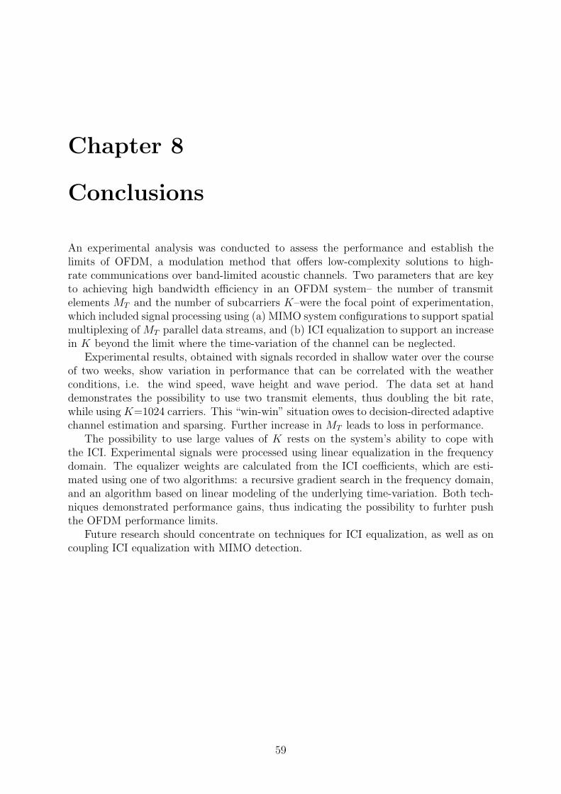
Chapter 8

Conclusions

An experimental analysis was conducted to assess the performance and establish thelimits of OFDM, a modulation method that offers low-complexity solutions to high-rate communications over band-limited acoustic channels. Two parameters that are keyto achieving high bandwidth efficiency in an OFDM system– the number of transmitelements MT and the number of subcarriers K–were the focal point of experimentation,which included signal processing using (a) MIMO system configurations to support spatialmultiplexing of MT parallel data streams, and (b) ICI equalization to support an increasein K beyond the limit where the time-variation of the channel can be neglected.

Experimental results, obtained with signals recorded in shallow water over the courseof two weeks, show variation in performance that can be correlated with the weatherconditions, i.e. the wind speed, wave height and wave period. The data set at handdemonstrates the possibility to use two transmit elements, thus doubling the bit rate,while using K=1024 carriers. This “win-win” situation owes to decision-directed adaptivechannel estimation and sparsing. Further increase in MT leads to loss in performance.

The possibility to use large values of K rests on the system’s ability to cope withthe ICI. Experimental signals were processed using linear equalization in the frequencydomain. The equalizer weights are calculated from the ICI coefficients, which are esti-mated using one of two algorithms: a recursive gradient search in the frequency domain,and an algorithm based on linear modeling of the underlying time-variation. Both tech-niques demonstrated performance gains, thus indicating the possibility to furhter pushthe OFDM performance limits.

Future research should concentrate on techniques for ICI equalization, as well as oncoupling ICI equalization with MIMO detection.

59

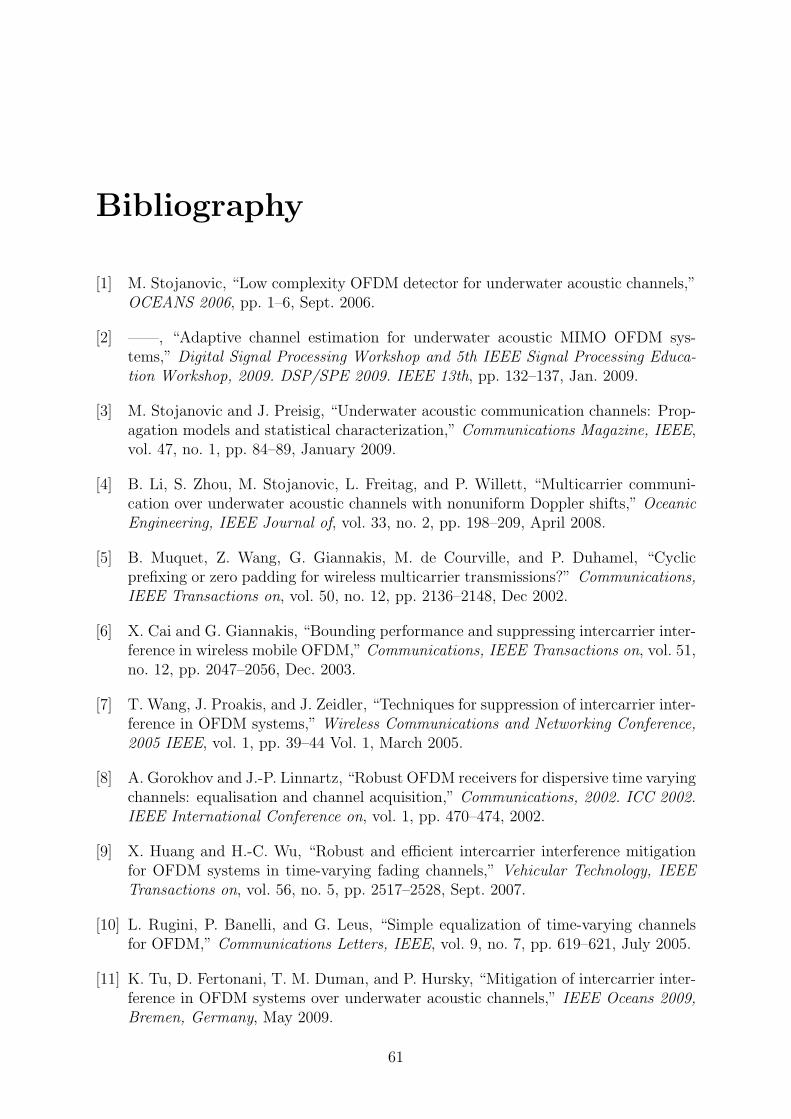
Bibliography

[1] M. Stojanovic, “Low complexity OFDM detector for underwater acoustic channels,”OCEANS 2006, pp. 1–6, Sept. 2006.

[2] ——, “Adaptive channel estimation for underwater acoustic MIMO OFDM sys-tems,” Digital Signal Processing Workshop and 5th IEEE Signal Processing Educa-tion Workshop, 2009. DSP/SPE 2009. IEEE 13th, pp. 132–137, Jan. 2009.

[3] M. Stojanovic and J. Preisig, “Underwater acoustic communication channels: Prop-agation models and statistical characterization,” Communications Magazine, IEEE,vol. 47, no. 1, pp. 84–89, January 2009.

[4] B. Li, S. Zhou, M. Stojanovic, L. Freitag, and P. Willett, “Multicarrier communi-cation over underwater acoustic channels with nonuniform Doppler shifts,” OceanicEngineering, IEEE Journal of, vol. 33, no. 2, pp. 198–209, April 2008.

[5] B. Muquet, Z. Wang, G. Giannakis, M. de Courville, and P. Duhamel, “Cyclicprefixing or zero padding for wireless multicarrier transmissions?” Communications,IEEE Transactions on, vol. 50, no. 12, pp. 2136–2148, Dec 2002.

[6] X. Cai and G. Giannakis, “Bounding performance and suppressing intercarrier inter-ference in wireless mobile OFDM,” Communications, IEEE Transactions on, vol. 51,no. 12, pp. 2047–2056, Dec. 2003.

[7] T. Wang, J. Proakis, and J. Zeidler, “Techniques for suppression of intercarrier inter-ference in OFDM systems,” Wireless Communications and Networking Conference,2005 IEEE, vol. 1, pp. 39–44 Vol. 1, March 2005.

[8] A. Gorokhov and J.-P. Linnartz, “Robust OFDM receivers for dispersive time varyingchannels: equalisation and channel acquisition,” Communications, 2002. ICC 2002.IEEE International Conference on, vol. 1, pp. 470–474, 2002.

[9] X. Huang and H.-C. Wu, “Robust and efficient intercarrier interference mitigationfor OFDM systems in time-varying fading channels,” Vehicular Technology, IEEETransactions on, vol. 56, no. 5, pp. 2517–2528, Sept. 2007.

[10] L. Rugini, P. Banelli, and G. Leus, “Simple equalization of time-varying channelsfor OFDM,” Communications Letters, IEEE, vol. 9, no. 7, pp. 619–621, July 2005.

[11] K. Tu, D. Fertonani, T. M. Duman, and P. Hursky, “Mitigation of intercarrier inter-ference in OFDM systems over underwater acoustic channels,” IEEE Oceans 2009,Bremen, Germany, May 2009.

61

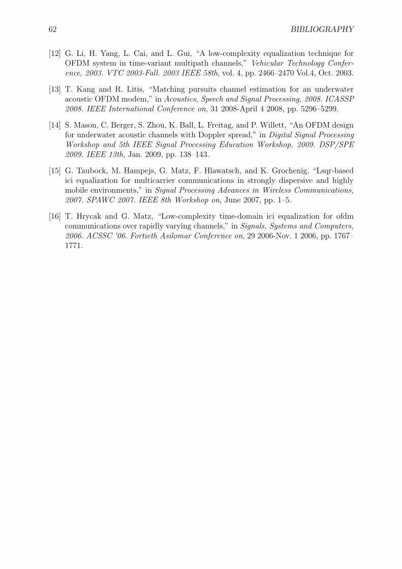
62 BIBLIOGRAPHY

[12] G. Li, H. Yang, L. Cai, and L. Gui, “A low-complexity equalization technique forOFDM system in time-variant multipath channels,” Vehicular Technology Confer-ence, 2003. VTC 2003-Fall. 2003 IEEE 58th, vol. 4, pp. 2466–2470 Vol.4, Oct. 2003.

[13] T. Kang and R. Litis, “Matching pursuits channel estimation for an underwateracoustic OFDM modem,” in Acoustics, Speech and Signal Processing, 2008. ICASSP2008. IEEE International Conference on, 31 2008-April 4 2008, pp. 5296–5299.

[14] S. Mason, C. Berger, S. Zhou, K. Ball, L. Freitag, and P. Willett, “An OFDM designfor underwater acoustic channels with Doppler spread,” in Digital Signal ProcessingWorkshop and 5th IEEE Signal Processing Education Workshop, 2009. DSP/SPE2009. IEEE 13th, Jan. 2009, pp. 138–143.

[15] G. Taubock, M. Hampejs, G. Matz, F. Hlawatsch, and K. Grochenig, “Lsqr-basedici equalization for multicarrier communications in strongly dispersive and highlymobile environments,” in Signal Processing Advances in Wireless Communications,2007. SPAWC 2007. IEEE 8th Workshop on, June 2007, pp. 1–5.

[16] T. Hrycak and G. Matz, “Low-complexity time-domain ici equalization for ofdmcommunications over rapidly varying channels,” in Signals, Systems and Computers,2006. ACSSC ’06. Fortieth Asilomar Conference on, 29 2006-Nov. 1 2006, pp. 1767–1771.