Two-Layer Linear Processing for MassiveMIMO on the TitanMIMO Platform
Sébastien RoyDept. of Electrical and Computer Engineering
Université de Sherbrookee-mail: [email protected]
January 27, 2015
Massive MIMO is a cornerstone technology in reaching the 5G target of a thousand-fold capacity increase by 2020. The paradigm is based on the fact that if there areenough antennas at the base station (several hundreds to a thousand or more), theso-called massive effect is observed whereby simple linear processing (eigenbeam-forming and maximal-ratio combining) becomes optimal. This is attractive becausesuch processing is not only extremely simple, it scales linearly with the size of the ar-ray and requires very little inter-processor communication. However, while antennasare not in themselves costly, such very large arrays with hundreds or thousands of RFfront-ends, A/D and D/A converters are cumbersome and energy-hungry, to say theleast. It is therefore of interest to explore the quasi-massive case, where the numberof antennas is not sufficient to achieve the massive effect, but still large enough tomake full-fledged interference nulling processing — such as minimum mean-squareerror (MMSE) and zero forcing (ZF) — undesirable because their complexity scalesin polynomial fashion, according to the cube of the number of antennas. We showhere that applying MMSE or ZF on subsets of antennas and further combining theresulting outputs in a second layer of processing constitutes an attractive approach toachieve good performance with reduced numbers of antennas, while limiting com-plexity. Furthermore, this approach maps extremely well to the TitanMIMO modulararchitecture where remote radio head (RRH) units of 8 antennas, each equipped withlocal baseband processing capability, are aggregated together to form massive MIMOprototyping platforms of various sizes.
1

1 What is massive MIMO?
The massive MIMO (multi-input, multi-output) paradigm is an evolution of multi-user MIMO(MU-MIMO). It should be understood that MIMO, in current wireless standards such as LTE and802.11, is typically implemented in its single-user form. That is to say that on a given channeland in a given timeslot, all the base station antennas are used to communicate with a single userterminal, itself being equipped with multiple antennas, where the multiplicity of antennas at bothends allows the creation of multiple data streams in space, thus multiplying the link capacity by asignificant factor. As it is easier to have a lot of antennas (for size and cost reasons) at the basestation compared to the handset, these additional degrees of freedom can be used to communicatewith multiple users at the same time, giving rise to MU-MIMO. However, this is a much moredifficult problem given that the multiple users addressed simultaneously cannot easily performjoint processing in order to eliminate the inter-user interference created with this method.
Therefore, while MU-MIMO is supported in LTE release 8, the precoding scheme therein doesnot completely address the interference problem. It follows that efficient implementation requiresclever processing beyond what is dictated by the standard, and many system designers are skepticalwith this route. The reason is that it is much simpler to maximize single-user MIMO (SU-MIMO)throughput, thus liberating the channels sooner for other users, rather than attempt MU-MIMOwhile the system gains are similar.
Given this state of affairs, neither SU-MIMO nor MU-MIMO is sufficiently powerful to achievethe 1000× capacity increase demanded by 5G. The seminal paper by Marzetta [1] introduced theconcept of “massive MIMO” in 2010 (also referred to as large-scale antenna systems or LSAS),generating immediate interest and numerous other papers [2]–[4]. It constitutes a theoretical andasymptotic analysis of a multi-cell scenario where a population of single-antenna terminals areserved by cellular base stations having an infinite number of antennas. While some real-worldconstraints are not considered, this work provides useful insights into the benefits and drawbacksof LSAS. Namely, when the number of base station antennas is allowed to tend towards infinity,
1. the effect of uncorrelated noise and fast fading vanish;
2. throughput and the number of terminals become independent from the size of the cells;
3. the required transmitted energy tends towards zero (due to infinite array gain);
4. multi-user interference vanishes; and
5. very simple forms of detection and precoding, namely matched filtering and eigenbeamform-ing, become optimal.
However, such theoretical fundamental benefits cannot be achieved without overcoming multiplepractical hurdles. Known issues affecting massive MIMO include
1. Pilot contamination: In massive MIMO, it is unrealistic to operate in FDD mode and touse some sort of sounding / feedback technique to obtain downlink channel estimates, given
2

the staggering overhead this would entail for such a large array. TDD operation is generallyassumed, with a frame size such that decent downlink channel estimates can be obtained byreciprocity from the uplink channel estimates. Typically, the latter are obtained during a ded-icated training interval, or, equivalently using pilot symbols. The pilots or training sequencescan be made orthogonal or quasi-orthogonal among users for a single cell, but will necessar-ily be contaminated by transmissions (re-use of training sequences) from surrounding cells.This effect, which does not diminish with the size of the array L, is widely recognized as oneof the main practical capacity limitations of the massive MIMO paradigm.
2. Array scale: The sheer array scale required to achieve the true massive effect, wherebyeigenbeamforming and maximal-ratio combining can be leveraged, involves staggering size,cost, and energy consumption considerations.
3. Array coherence: Appropriate synchronization, calibration, and phase alignment accross alarge-scale array, of hundreds of antennas or more, pose serious practical challenges.
To summarize, the true massive effect implies that eigenbeamforming and maximal-ratio com-bining are optimal, transmit power can be made arbitrarily small, white noise, channel estimationerror and interference vanish, and capacity is limited by pilot contamination. This is known toresult when the base station array size L tends towards ∞ while the number of addressed userantennas M remains fixed. Obviously, a limit must be imposed on the size of the array in practice,as expressed by hurdle 2 above. Hoydis, ten Brink and Debbah have asked the important ques-tion “How many antennas to we need?” in practice in order to achieve a significant percentageof the ideal massive MIMO performance [5]. They show therein that in certain scenarios, ZF andMMSE processing can attain the performance level of eigenbeamforming / MRC with an order ofmagnitude fewer antennas. However, the resulting array must still be large with respect to the userpopulation of size M , and the complexity of ZF and MMSE raises serious concerns given that itscales according to L3 and that processing accross the entire array becomes tightly intercoupled,requiring rapid and flexible connections between local baseband processors.
A key paper [6] describes Argos, the first (and one of the few) hardware implementation of anLSAS hardware system in the spirit of massive MIMO. This reference is crucial because in theprocess of making a working system, based on a modular, scalable architecture, the authors hadto address (and describe therein) the main practical issues associated with such an undertaking.The system needed to be scalable both in terms of numerical complexity and in terms of datarouting requirements. Indeed, as the array becomes very large, it becomes impractical (in termsof hardware complexity and / or delay) to gather data from all antennas in one central locationfor weight calculation, detection and / or channel estimation. Thus, all these tasks must ideallybe performed locally at each antenna, and their numerical complexity should scale linearly withthe number of antennas. The prototype system comprises one FPGA processing board for every 4antennas, so its computation power does scale linearly as well. In order to achieve this, the authorsused conjugate (matched) beamforming with local power scaling, so that channel estimation andweight computation can be performed locally. Furthermore, internal calibration is implementedrelative to antenna 1, and this is shown to be adequate to compensate for the effect of RF component
3

imperfections on channel reciprocity. However, their results show that zero-forcing beamformingyields a capacity advantage by a factor of 2 to 4 for the relatively small number of antennas (16to 64) used in the experiment. This confirms the results of [5] discussed above. Thus, many moreantennas (100s) would be required for conjugate beamforming to become optimal, yet zero-forcinghas a numerical complexity that scales with L3 (due to matrix inversion) and requires data routingto a central controller for weight computation.
The Nutaq TitanMIMO platform [7] represents a significant evolution with respect to Argos inmany respects. It provides one large Virtex-6 FPGA for every 8 antennas, with all modules beinglinked in a user-defined topology with high speed point-to-point links (up to 7x 20Gbps links permodule). The latter enable the testbed to be used in a wide range of scenarios making it a perfect fitfor massive MIMO/multi-layer processing research-oriented projects. Figure 1 shows an exampleof a TitanMIMO system which supports up to 64 RF transceivers, using an RRH-only topology.
Figure 1: TitanMIMO-6S 64 TRX configuration
Since each module (RRH) possesses 7 high speed point-to-point links, a large number of dif-ferent topologies can be implemented. However, as the number of antennas increases, additionalprocessing power is required and there comes a point where the local processing of the RRH mod-ules may not suffice. However, the scalability of the TitanMIMO can be pushed further by addingone or more octal-FPGA central processing boards (Kermode XV6) as shown in Figs. 2 and 3.
This scalability can attain up to 1000 TX/RX channels and the additional processing powerbrought by the Octal-FPGA processing boards enables the implementation of higher complexityalgorithms such as ZF and MMSE.
2 Two-layer processing
Given large-scale arrays of manageable sizes in practice, the above discussion highlights the needfor algorithms that are simpler and that scale better than full-fledged ZF or MMSE, while offering
4

Figure 2: TitanMIMO-6D 128 TRX configuration
Figure 3: TitanMIMO-6D 256 TRX configuration
better interference nulling than eigenbeamforming / MRC. One promising approach on the recep-tion side is to form subsets of antennas of a given size N , to apply ZF or MMSE at the subsetlevel (the first processing layer), and to subsequently combine the resulting outputs using MRC(second processing layer). In this approach complexity is essentially proportional toN3, instead of
5

L3, where N can be made much smaller than L, according to the desired complexity-performancetradeoff. It should be noted that while N is assumed fixed in the following, it is entirely possible tohave subsets of unequal size, which might in fact be necessary for certain array sizes L dependingon the number of desired subsets.
...
Base station
L
M
Figure 4: Typical massive MIMO scenario: the base station has L antennas and is servicing Msingle-antenna terminals, where L�M .
Figure 4 shows a typical massive MIMO scenario where the base station is equipped with a largenumber L of antennas and is servicing a population of M single-antenna user terminals on anygiven channel, where L is assumed to be at least an order of magnitude greater than M . Thus, thecomplex baseband model of this MIMO link is given by
x = Hs + n, (1)
where x ∈ CL×1 is the received signal and H ∈ CL×M is the Rayleigh-fading channel matrixcomprised of independent, identically distributed (i.i.d.) zero-mean circularly symmetric complexGaussian coefficients denoted by hml ∼ N(0, 1) for 1 ≤ m ≤ M , 1 ≤ l ≤ L. It is assumed thattheM data streams have equal power. In other words, s ∈ CM×1 is characterized by the followingcovariance matrix:
Rxx =⟨xxH
⟩= P IM , (2)
where 〈·〉 is the expectation operator, (·)H = (·)∗T is the Hermitian transpose (or conjugate trans-pose), and IM is the M ×M identity matrix. Finally, the thermal white Gaussian noise vectorn ∈ CL×1 is also circularly symmetric such that n ∼ N
(0, σ2nIL
).
For conventional linear processing on the uplink, the vector of estimates of the transmitted sig-nals prior to detection is given by
z = Wx, (3)
where each entry of z ∈ CM×1 corresponds to the same entry of s, and W ∈ CM×L is the weightcombining matrix. It should be noted that the mth row of W is the weight combining vector foruser m’s signal.
6

If we assume perfect channel knowledge, the weight combining matrix W for MRC, ZF andMMSE is given by
WMRC = HH , (4)
WZF =(HHH
)−1HH , (5)
WMMSE =
(HHH +
σ2nP
I
)−1
HH . (6)
It can be seen that both ZF and MMSE require matrix inversion, which for large array size Lbecomes problematic given that the complexity is O(L3). Meanwhile, MRC is much simpler toimplement but requires a much larger array to yield acceptable performance.
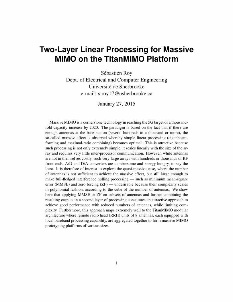
Figure 5 shows the proposed 2-layer processing scheme for reception (uplink) at the base station.Here, the processing for a single user is illustrated and the output is one of the entries of vector z.It should be understood that a similar structure can be leveraged for transmission (downlink) withidentical benefits. Therefore, we focus herein and without loss of generality on the uplink, theextension to downlink processing being straightforward.
With this architecture, all antennas in the array are equipped with an RF front-end (including A/Dand D/A conversion) and first layer processing in each group is performed in the digital domain.The first layer subset processors implement either ZF or MMSE combining in order to reduceinter-user interference. Thus, we have, for all users
yk = Wkxk, (7)
where 1 ≤ k ≤ K, xk is the portion of the received signal vector x corresponding to the kth subset,and Wk is the weight combining matrix associated with the latter. Thus, Wk is computed in oneof two ways, depending on whether ZF or MMSE processing is desired, i.e.
Wk =
Wk,ZF =(HHk Hk
)−1HHk for ZF,
Wk,MMSE =(HHk Hk + σ2
nP I)−1
HHk for MMSE,
(8)
where Hk ∈ CN×M is the portion of the channel matrix H corresponding to the kth subset.To apply MRC in the second layer, we recall that the MRC concept is akin to a spatial matched
filter, i.e. each input is co-phased and weighted proportionally to its SINR. It should be noted,however, that all inputs are already co-phased as a result of first-layer processing.
For a given user m, we have
ymk = wHmkxk,
= wHmkHks + wH
mknk, (9)
where the mth row of Hk will henceforth be denoted hmk.The final output of the two-layer processor for user m is given by
zm = w̄Hmy. (10)
7
Second layer
ZF / MMSE ZF / MMSEZF / MMSE ......
...MRC
Analog / RF domain
Digital domain
... ... ...
First layer
ym1 ym2 ymK
zm
N︷ ︸︸ ︷ N︷ ︸︸ ︷N︷ ︸︸ ︷L=KN︷ ︸︸ ︷
RF front end - A/D - D/A
{
Figure 5: Two-layer processing scheme for the uplink at the base station of a massive MIMOsystem
If zero-forcing is used in the first layer, we have
w̄m =
√hHm1
(HH
1 H1
)−1hm1√
hHm2
(HH
2 H2
)−1hm2
...√hHmK
(HHKHK
)−1hmK
, (11)
where hmk is the mth column of Hk or, equivalently, the channel coefficient vector for user m onsubset k.
Similarly, if MMSE is used in the first layer, we have
w̄m =
√hHm1
(HH
1 H1 + σ2nP I)−1
hm1√hHm2
(HH
2 H2 + σ2nP I)−1
hm2
...√hHmK
(HHKHK + σ2
nP I)−1
hmK
. (12)
If the signal-to-interference-plus-noise ratio (SINR) at the output of subset k for user m is de-noted γkm, then the final combined output at the second layer for user m will have an SINR of
γm =
K∑k=1
γkm. (13)
8
3 Performance comparisons
It should be noted that while many papers on massive MIMO present asymptotic, i.e. approximate,results in part due to the fact that simulations can become very time consuming and cumbersomeat large array sizes, all performance results herein for MRC and ZF combiners are exact.
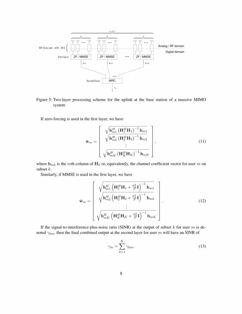
It has been established that as the number of antennas grows to infinity, thanks to the “massiveeffect,” MRC becomes the optimal combining method. However, at more modest array sizes, MRCsuffers from an error floor due to the fact that it does not null interference completely, regardless ofSNR. This is why ZF and MMSE combiners, which specifically target interferers, can achieve thesame performance as MRC at a much smaller array size.
SNR (dB)
ZFMRC
200
250
300350500
1000400
22100
4030
50
10−10 200−20
10−3
10−4
10−5
10−6
Bit
erro
rpro
babi
lityPe
1
10−1
10−2
Figure 6: Bit error probability versus SNR for MRC and ZF for various array sizes L when thenumber of received signals M = 20.
Figure 6 compares the error performance of MRC and ZF combiners for various array sizeswhile assuming a number of transmit antennas of M = 20. For analytical convenience (andwithout loss of generality since the trends and relationships between curves would be similar forany modulation type), DPSK modulation is assumed. It can be observed that to reach a performancelevel of Pe = 10−3 at a SNR of -10 dB (or Pe = 10−4 at a SNR of 10 dB), at least 200 antennas arerequired for MRC. To attain Pe = 10−3 at a SNR of -10 dB with ZF, however, 100 antennas is morethan enough. And, because there is no error floor, between 22 and 30 antennas would be adequateto reach Pe = 10−4 at 10 dB. Observing the crossing points of the curves is most informative. Forexample, at a SNR of 1.5 dB, a 30-antenna ZF array yields the same error probability as a 200-antenna MRC one. That is nearly a factor of 7 in array size. Likewise, at -3 dB, both a 50-antennaZF array and a 350-antenna MRC array yield an error probability of 10−6. Here, we have exactly
9
a factor of 7.It should be noted that the error performance of ZF and MMSE behaves in a very similar way, i.e.
the slope of their bit error rate (BER) curves is the same. However, MMSE has a slight advantage,typically on the order of a few dBs, which translates to a shift of the BER curve to the left. Itwas shown in [8] that there exists a performance gain in MMSE with respect to ZF that does notdiminish with increasing SNR. However, it is known that training converges faster with ZF thanwith MMSE, thus implying that ZF may not suffer as much in the presence of channel estimationerrors.
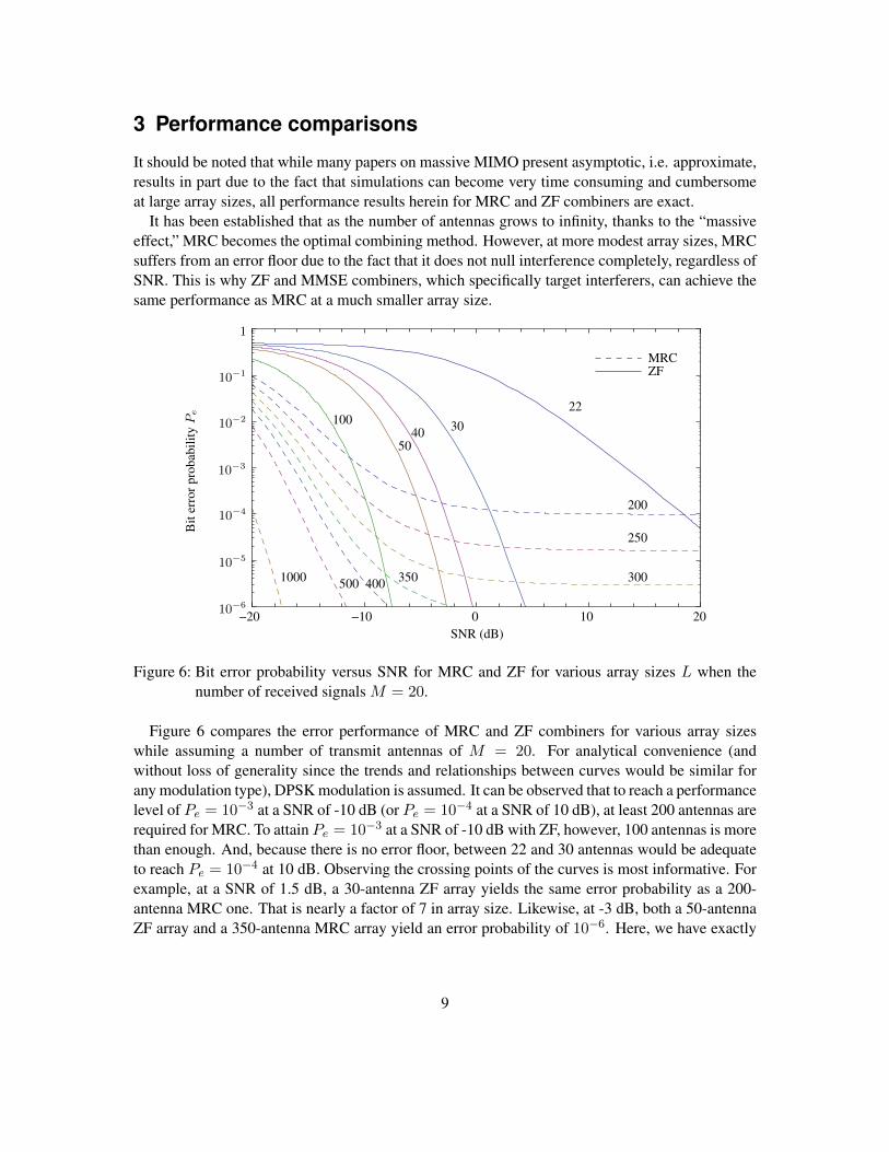
Figure 7 compares the performance of various types of combiners, including 3 instances of two-layer architectures with a number of signals M = 16. Given the TitanMIMO RRH size of 8, groupsizes of 16 were chosen for the two-layer schemes. Thus, each subset processor in layer 1 can beimplemented accross a pair of RRH units. It can be observed that to reach Pe = 10−3 at an SNRof 0 dB or better, at least 128 antennas are required with MRC. This same level of performanceis attained with only 32 antennas divided into 2 sets of 16 with ZF / MRC 2-layer processing atan SNR of 15 dB. If instead MMSE / MRC processing is used with 2 sets of 16, an SNR of 6 dBis sufficient. It can be seen that the 4 × 16 ZF / MRC curve has a steeper curve than the 2 × 16schemes, but it is poorer than the MMSE / MRC 2× 16 processor below 9 dB.
SNR (dB)
10−10 200−20
Bit
erro
rpro
babi
lityPe
ZF / MRC, 2× 16
2× 16
MMSE, L = 128 MMSE, L = 64
MMSE, L = 32
MRC, L = 64
MRC, L = 128
ZF / MRC4× 16
MMSE / MRC
1
10−1
10−2
10−3
10−4
10−5
10−6
Figure 7: Bit error probability versus SNR for various combiners when the number of receivedsignals M = 16.
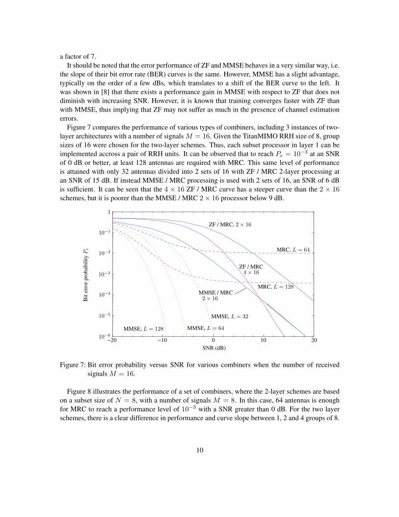
Figure 8 illustrates the performance of a set of combiners, where the 2-layer schemes are basedon a subset size of N = 8, with a number of signals M = 8. In this case, 64 antennas is enoughfor MRC to reach a performance level of 10−3 with a SNR greater than 0 dB. For the two layerschemes, there is a clear difference in performance and curve slope between 1, 2 and 4 groups of 8.
10

10−10 200−20
SNR (dB)
MRC, L = 128
ZF, L = 64
ZF, L = 32
ZF, L = 16
MMSE, L = 8
ZF, L = 8
ZF/MRC, 2× 8
ZF/MRC, 4× 8
MRC, L = 64
1
10−1
10−2
10−3
10−4
10−5
10−6
Bit
erro
rpro
babi
lityPe
Figure 8: Bit error probability versus SNR for various combiners when the number of receivedsignals M = 8.
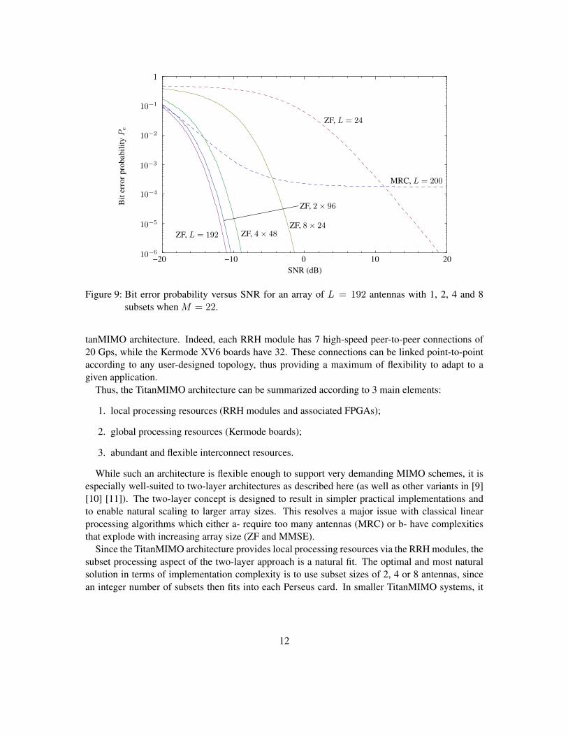
Figure 9 shows a different angle to performance comparison. Here, the number of impingingsignals is M = 22 and the subset size is either N = 24 (equivalent to 3 RRH modules in aTitanMIMO system) or a multiple thereof. While maintaining the array size at L = 192, we varythe number of subsets from 1 to 8. Curves for MRC with L = 200 and ZF with L = 24 areprovided for reference purposes. Going from full ZF with 192 antennas (with a complexity ofO(1923)) to 2 subsets of 96 antennas (with a complexity of O(963)), we see that the performancepenalty is less than 1 dB while the complexity is reduced by a factor of 23/2 = 4. Likewise, with4 subsets of 48, the performance penalty with respect to full ZF is approximately 2.5 dB while thecomplexity is reduced by a factor 43/4 = 16. With 8 subsets of 24, the performance penalty growsto 8 dB while the complexity reduction is on the order of 83/8 = 64.
4 Prototyping with TitanMIMO platform
The TitanMIMO architecture is designed to be modular and scalable, according to requirements.Processing is naturally distributed since each remote radio head (RRH) module of 8 RF transceiversis equipped with its own Virtex-6 FPGA (Perseus 611x card), and the collection of RRH modulescan be linked to one or more Kermode XV6 modules, each being equipped with superlative com-puting power (8 large FPGAs from the Virtex-6 family) and thus play the role of central processinunit(s).
As with all parallel computing systems, the performance keystone resides in the bandwidth andflexibility of the interconnection network. This is precisely one of the great strenghts of the Ti-
11
SNR (dB)
−20 0 20−10 10
ZF, L = 192
1
10−1
10−2
10−3
10−4
10−5
10−6
Bit
erro
rpro
babi
lityPe
MRC, L = 200
ZF, L = 24
ZF, 4× 48ZF, 8× 24
ZF, 2× 96
Figure 9: Bit error probability versus SNR for an array of L = 192 antennas with 1, 2, 4 and 8subsets when M = 22.
tanMIMO architecture. Indeed, each RRH module has 7 high-speed peer-to-peer connections of20 Gps, while the Kermode XV6 boards have 32. These connections can be linked point-to-pointaccording to any user-designed topology, thus providing a maximum of flexibility to adapt to agiven application.
Thus, the TitanMIMO architecture can be summarized according to 3 main elements:
1. local processing resources (RRH modules and associated FPGAs);
2. global processing resources (Kermode boards);
3. abundant and flexible interconnect resources.
While such an architecture is flexible enough to support very demanding MIMO schemes, it isespecially well-suited to two-layer architectures as described here (as well as other variants in [9][10] [11]). The two-layer concept is designed to result in simpler practical implementations andto enable natural scaling to larger array sizes. This resolves a major issue with classical linearprocessing algorithms which either a- require too many antennas (MRC) or b- have complexitiesthat explode with increasing array size (ZF and MMSE).
Since the TitanMIMO architecture provides local processing resources via the RRH modules, thesubset processing aspect of the two-layer approach is a natural fit. The optimal and most naturalsolution in terms of implementation complexity is to use subset sizes of 2, 4 or 8 antennas, sincean integer number of subsets then fits into each Perseus card. In smaller TitanMIMO systems, it
12
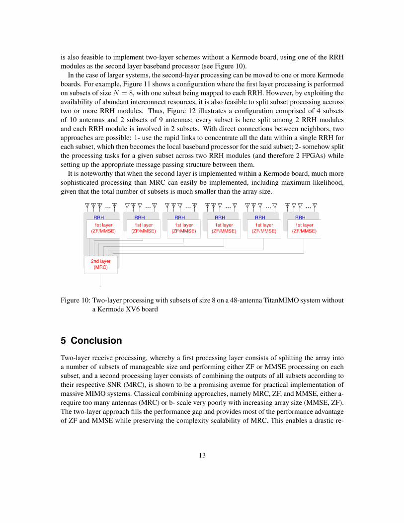
is also feasible to implement two-layer schemes without a Kermode board, using one of the RRHmodules as the second layer baseband processor (see Figure 10).
In the case of larger systems, the second-layer processing can be moved to one or more Kermodeboards. For example, Figure 11 shows a configuration where the first layer processing is performedon subsets of size N = 8, with one subset being mapped to each RRH. However, by exploiting theavailability of abundant interconnect resources, it is also feasible to split subset processing accrosstwo or more RRH modules. Thus, Figure 12 illustrates a configuration comprised of 4 subsetsof 10 antennas and 2 subsets of 9 antennas; every subset is here split among 2 RRH modulesand each RRH module is involved in 2 subsets. With direct connections between neighbors, twoapproaches are possible: 1- use the rapid links to concentrate all the data within a single RRH foreach subset, which then becomes the local baseband processor for the said subset; 2- somehow splitthe processing tasks for a given subset across two RRH modules (and therefore 2 FPGAs) whilesetting up the appropriate message passing structure between them.
It is noteworthy that when the second layer is implemented within a Kermode board, much moresophisticated processing than MRC can easily be implemented, including maximum-likelihood,given that the total number of subsets is much smaller than the array size.
RRH RRHRRHRRHRRHRRH
1st layer
(ZF/MMSE)
1st layer
(ZF/MMSE)(ZF/MMSE)
1st layer
(ZF/MMSE)
1st layer
(MRC)
2nd layer
1st layer
(ZF/MMSE)
1st layer
(ZF/MMSE)
Figure 10: Two-layer processing with subsets of size 8 on a 48-antenna TitanMIMO system withouta Kermode XV6 board
5 Conclusion
Two-layer receive processing, whereby a first processing layer consists of splitting the array intoa number of subsets of manageable size and performing either ZF or MMSE processing on eachsubset, and a second processing layer consists of combining the outputs of all subsets according totheir respective SNR (MRC), is shown to be a promising avenue for practical implementation ofmassive MIMO systems. Classical combining approaches, namely MRC, ZF, and MMSE, either a-require too many antennas (MRC) or b- scale very poorly with increasing array size (MMSE, ZF).The two-layer approach fills the performance gap and provides most of the performance advantageof ZF and MMSE while preserving the complexity scalability of MRC. This enables a drastic re-
13

RRH RRH
Processor CoreBasebandOctal V6
RRH RRH RRH RRH RRH RRH
(ZF/MMSE) (ZF/MMSE)
(MRC)
2nd layer
(ZF/MMSE)
1st layer 1st layer1st layer 1st layer
(ZF/MMSE) (ZF/MMSE)
1st layer
(ZF/MMSE)
1st layer
(ZF/MMSE)
1st layer
(ZF/MMSE)
1st layer
Figure 11: Two-layer processing with subsets of size N = 8 on a 64-antenna TitanMIMO system
RRH
Processor CoreBasebandOctal V6
RRH RRH RRH RRH RRH RRHRRH
1st layer 1st layer
(MRC)
2nd layer
(ZF/MMSE)
1st layer
(ZF/MMSE)
1st layer
(ZF/MMSE)
1st layer
(ZF/MMSE)
1st layer
(ZF/MMSE) (ZF/MMSE)
Figure 12: Two-layer processing with subsets of size 8 and 9 on a 64-antenna TitanMIMO system
duction in the number of antennas and RF chains with respect to MRC for similar performancelevels. Since this approach is inherently modular, it maps naturally to the TitanMIMO architecture.Furthermore, a TitanMIMO with two-layer processing can be scaled up with predictable and man-ageable complexity growth. Thus, 2-layer processing can be implemented on a small system whichcan be incrementally upgraded to larger array sizes with minimal changes to FPGA configurations.
References
[1] T. L. Marzetta, “Noncooperative cellular wireless with unlimited num- bers of base stationantennas,” IEEE Trans. Wireless Commun., vol. 9, no. 11, pp. 3590–3600, Nov. 2010.
[2] A. Pitarokoilis, S. K. Mohammed, and E. G. Larsson, “On the Optimality of Single-CarrierTransmission in Large-Scale Antenna Systems,” IEEE Wireless Commun. Lett., vol. 1, no. 4,pp. 276-279, Aug. 2012.
[3] F. Rusek, D. Persson, B. K. Lau, E. G. Larsson, T. L. Marzetta, O. Edfors, and F. Tufvesson,
14

“Scaling up MIMO: Opportunities and Challenges with Very Large Arrays,” IEEE SignalProcess. Mag., to appear, 2012.
[4] B. Gopalakrishnan and N. Jindal, “An Analysis of Pilot Contamination on Multi-User MIMOCellular Systems with Many Antennas,” Proc. Signal Processing Advances in Wireless Com-munications (SPAWC), San Francisco, CA, June 2011.
[5] J. Hoydis, S. Ten Brink, and M. Debbah, “Massive MIMO in the UL/DL of cellular networks:How many antennas do we need?,” IEEE Journal on Selected Areas in Communications, vol.31, no. 2, pp. 160–171, Feb. 2013.
[6] C. Shepard, H. Yu, N. Anand, L. E. Li, T. L. Marzetta, R. Yang, and L. Zhong, “Argos: practi-cal many-antenna base stations,” in Proc. ACM Int. Conf. Mobile Computing and Networking(MobiCom), Aug. 2012.
[7] M. Brown and M. Turgeon, “TitanMIMO: A 100x100 Massive MIMO Testbed Based onxTCA Standards,” white paper, Nutaq Inc., www.nutaq.com.
[8] Y. Jiang, M. K. Varanasi, and J. Li, “Performance analysis of ZF and MMSE equalizers forMIMO systems: an in-depth study of the high SNR regime,” IEEE Transactions on Informa-tion Theory, vol. 57, no. 4, pp. 2008–2026, April 2011.
[9] S. Roy, “Dual layer switch-and-examine / selection diversity receivers,” IEEE Vehicular Tech-nology Conference (VTC) – Spring, Dresden, Germany, June 2–5, 2013.
[10] S. Roy, “Performance analysis of hierarchical selection diversity combining in Rayleigh fad-ing,” International Conference on Networking and Communications (ICNC), San Diego,U.S.A., Jan 28–31, 2013.
[11] S. Roy, “Hierarchical Selection Diversity Combining Architecture,” IEEE Int. Conf. on Com-mun. (ICC), Ottawa, Canada, June 10–15, 2012.
15

Biography
Sébastien Roy is professor at the Departement of Electrical and Computer Engineering at Uni-versité de Sherbrooke, Sherbrooke, Canada, as well as founder and head of the World-MachineInterface Research Group (WMIRG). He has published over 120 journal and conference papers,most of which are in the field of wireless communications and, more specifically, antenna arraysand MIMO systems. Active in technology transfer and industrial consulting, he holds 7 patents inthe US and worldwide. He recently received the VTS Conference Chair Award, jointly with co-chair André Morin, for chairing the Vehicular Technology Conference (VTC) Fall 2012 in QuebecCity.
16
Recommended