Lappeenrannan teknillinen yliopisto Lappeenranta University of Technology
Panu Kurronen TORQUE VIBRATION MODEL OF AXIAL-FLUX SURFACE-MOUNTED PERMANENT MAGNET SYNCHRONOUS MACHINE
Thesis for the degree of Doctor of Science (Technology) to be presented with due permission for public examination and criticism in the Auditorium 1383 at Lappeenranta University of Technology, Lappeenranta, Finland on the 22nd of August, 2003, at noon.
Acta Universitatis Lappeenrantaensis 154
ISBN 951-764-773-5 ISSN 1456-4491
Lappeenrannan teknillinen yliopisto
Digipaino 2003
ABSTRACT
Lappeenranta University of Technology Acta Universitatis Lappeenrantaesis 154 Panu Kurronen Torque vibration model of axial-flux surface-mounted permanent magnet synchronous machine Lappeenranta 2003 ISBN 951-764-773-5, ISSN 1456-4991
In order that the radius and thus ununiform structure of the teeth and other electrical and mag-
netic parts of the machine may be taken into consideration the calculation of an axial flux per-
manent magnet machine is, conventionally, done by means of 3D FEM-methods. This calcula-
tion procedure, however, requires a lot of time and computer recourses. This study proves that
also analytical methods can be applied to perform the calculation successfully. The procedure of
the analytical calculation can be summarized into following steps: first the magnet is divided
into slices, which makes the calculation for each section individually, and then the parts are
submitted to calculation of the final results. It is obvious that using this method can save a lot of
designing and calculating time.
The calculation program is designed to model the magnetic and electrical circuits of surface
mounted axial flux permanent magnet synchronous machines in such a way, that it takes into
account possible magnetic saturation of the iron parts. The result of the calculation is the torque
of the motor including the vibrations. The motor geometry and the materials and either the
torque or pole angle are defined and the motor can be fed with an arbitrary shape and amplitude
of three-phase currents. There are no limits for the size and number of the pole pairs nor for
many other factors. The calculation steps and the number of different sections of the magnet are
selectable, but the calculation time is strongly depending on this. The results are compared to
the measurements of real prototypes.
The permanent magnet creates part of the flux in the magnetic circuit. The form and amplitude
of the flux density in the air-gap depends on the geometry and material of the magnetic circuit,
on the length of the air-gap and remanence flux density of the magnet. Slotting is taken into ac-
count by using the Carter factor in the slot opening area.
The calculation is simple and fast if the shape of the magnet is a square and has no skew in rela-
tion to the stator slots. With a more complicated magnet shape the calculation has to be done in
several sections. It is clear that according to the increasing number of sections also the result
will become more accurate. In a radial flux motor all sections of the magnets create force with a
same radius. In the case of an axial flux motor, each radial section creates force with a different
radius and the torque is the sum of these.
The magnetic circuit of the motor, consisting of the stator iron, rotor iron, air-gap, magnet and
the slot, is modelled with a reluctance net, which considers the saturation of the iron. This
means, that several iterations, in which the permeability is updated, has to be done in order to
get final results.
The motor torque is calculated using the instantaneous linkage flux and stator currents. Flux
linkage is called the part of the flux that is created by the permanent magnets and the stator cur-
rents passing through the coils in stator teeth. The angle between this flux and the phase cur-
rents define the torque created by the magnetic circuit.
Due to the winding structure of the stator and in order to limit the leakage flux the slot openings
of the stator are normally not made of ferromagnetic material even though, in some cases,
semimagnetic slot wedges are used. In the slot opening faces the flux enters the iron almost
normally (tangentially with respect to the rotor flux) creating tangential forces in the rotor. This
phenomenon is called cogging. The flux in the slot opening area on the different sides of the
opening and in the different slot openings is not equal and so these forces do not compensate
each other. In the calculation it is assumed that the flux entering the left side of the opening is
the component left from the geometrical centre of the slot. This torque component together with
the torque component calculated using the Lorenz force make the total torque of the motor.
It is easy to assume that when all the magnet edges, where the derivative component of the
magnet flux density is at its highest, enter the slot openings at the same time, this will have as a
result a considerable cogging torque. To reduce the cogging torque the magnet edges can be
shaped so that they are not parallel to the stator slots, which is the common way to solve the
problem. In doing so, the edge may be spread along the whole slot pitch and thus also the high
derivative component will be spread to occur equally along the rotation.
Besides forming the magnets they may also be placed somewhat asymmetric on the rotor sur-
face. The asymmetric distribution can be made in many different ways. All the magnets may
have a different deflection of the symmetrical centre point or they can be for example shifted in
pairs. There are some factors that limit the deflection. The first is that the magnets cannot over-
lap. The magnet shape and the relative width compared to the pole define the deflection in this
case. The other factor is that a shifting of the poles limits the maximum torque of the motor. If
the edges of adjacent magnets are very close to each other the leakage flux from one pole to the
other increases reducing thus the air-gap magnetization.
The asymmetric model needs some assumptions and simplifications in order to limit the size of
the model and calculation time. The reluctance net is made for symmetric distribution. If the
magnets are distributed asymmetrically the flux in the different pole pairs will not be exactly
the same. Therefore, the assumption that the flux flows from the edges of the model to the next
pole pairs, in the calculation model from one edge to the other, is not correct. If it were wished
for that this fact should be considered in multi-pole pair machines, this would mean that all the
poles, in other words the whole machine, should be modelled in reluctance net. The error result-
ing from this wrong assumption is, nevertheless, irrelevant.
UDC 621.313.323 : 621.318.2
Keywords: Permanent magnet synchronous machine, Axial-flux, tangential vibration

ACKNOWLEDGEMENTS
I wish thank all the parties who have promoted the progress of this thesis.
First I would like express my great gratitude for my supervisor Professor Juha Pyrhönen for
creating the preconditions to carry out this study and for all his support and interest in the work.
Also the good advice of the supporting team Markku Niemelä, Janne Nerg and Jussi Salo is
considered with gratefulness. Asko Parviainen I wish to thank for the calculation support and
the laboratory team Jouni Ryhänen, Harri Loisa and Martti Lindh for the measurement
arrangements.
The financial support by IVO-foundation (at present Fortum foundation), Ulla Tuominen
foundation, Tekniikan editämissäätiö, National Technology Agency of Finland, Finnish
Academy, Metso Paper Oyj and ABB Industry Oy is highly appreciated. Kone Corporation and
there especially Tarvo Viita-aho I thank for material and technical support.
I’m much obliged to Professor Tapani Jokinen and Dr. Eero Keskinen for valuable comments
and corrections and Julia Vauterin for language review during pre examination.
Most of all I wish express my gratefulness to my family Kirsi, Laura, Henni and Jesse for
standing beside me during these rough years. I love you.
Lappeenranta 31th of June 2003 Panu Kurronen

CONTENTS ABSTRACT
ACKNOWLEDGEMENTS
CONTENTS
ABBREVIATIONS AND VARIABLES
1 INTRODUCTION 15 1.1 Existing Calculation Methods 17 1.2 Mechanical System Vibrations 18 1.3 Permanent Magnet Synchronous Motor 20
1.3.1 The Development and the Features of the Permanent Magnet Material 21 1.3.2 Permanent Magnet Synchronous Motor (PMSM) types 24
1.4 Frequency Converter 30 1.5 Outline of the Thesis 31 1.6 The Scientific Contribution of This Work 33
2 TORQUE CALCULATION MODEL 34 2.1 General 34 2.2 Air-Gap Flux Created by the Permanent Magnets 35 2.3 Magnetic Circuit 40 2.4 Torque Calculation 42
2.4.1 Flux Linkage 43 2.5 Cogging Torque 45 2.6 Radial Flux and Axial Flux Motor Calculation 47 2.7 Calculation Procedure 47 2.8 Conclusions 50
3 TORQUE VIBRATION 51 3.1 Calculation Parameters 52 3.2 Stator 54
3.2.1 Slotting and Slot Opening 55 3.2.2 Winding Harmonics 60
3.3 Air-gap 66 3.4 The Rotor 67
3.4.1 Permanent Magnets 67 3.5 Magnetic Circuit and Saturation 81 3.6 Asymmetric Magnetic Circuits 83
3.6.1 Asymmetric Magnet Distribution 85 3.6.2 Additional Slot or Slots 88 3.6.3 Eccentricity 89
3.7 Conclusions 89
4 MODEL VERIFICATION – EXPERIMENTAL RESULTS 90 4.1 Reference Motor Versions 90 4.2 Reference Motor Calculations 91
4.2.1 Comparison Between FEM and Analytical Calculation 93 4.3 Test Setup 101 4.4 Comparison Between Calculations and Measurements 104
4.4.1 Standard Stator 104 4.4.2 The Influence of the Additional Slot Stator 106 4.4.3 Measured and Calculated Air-gap Permeance Harmonic Torque 107 4.4.4 Current Asymmetry Effects 108
4.5 Conclusions of Comparison 110
5 CONCLUSIONS 112
REFERENCES 114
APPENDIX A 118
ABBREVIATIONS AND VARIABLES
ABBREVIATIONS
2D Two-dimensional
3D Three-dimensional
ABB DCS 500 ABB DC-converter tm
AFPMSM Axial flux permanent magnet synchronous motor
CCW Counter clockwise
CW Clockwise
DC Direct current
DTC Direct Torque Control
FEM Finite Element Method
T/I Torque-Current -ratio
IM Induction motor
mmf Magneto motive force
NdFeB Neodym Iron Boron -alloy
PM1 Permanent magnet shape
PM2 Permanent magnet shape
PM3 Permanent magnet shape
PMSM Permanent magnet synchronous machine
SOR Sector of a ring
RMS Root mean square
SM Synchronous motors
SmCo Samarium Cobalt -alloy
VARIABLES
[NI] MMF matrix.
[R] Reluctance matrix
B Flux density
BHmax Energy product
Bpm Permanent magnet remanence flux density
Br Remanence flux density
E Electric field strength
f Frequency
fs Rated supply frequency
g1 Positive or negative integer.
ga Length variable
H Field strength
Hc Coercive force
Hc’ Coercivity
hpm Magnet thickness
hso Slot opening height
hto Tooth height
i Peak current
I RMS current
id Direct axis current
In Motor rated current
JHC Coersivity
kw Constant.
Lsc The length of the stator stack
m Number of phases
n Number of poles
nc Number of coils
NI Total current of each individual coil
Ns Number of turns in a slot
p Number of pole pairs
Pn Motor rated power
Q Charge
q Number of slots per pole and phase
Qs Number of slots
r Radius
R Reluctance
rag Average air-gap radius
rm, Permanent magnet outer radius (radial flux motor)
rr Rotor radius (radial flux motor)
rs Stator radius (radial flux motor)
ssg Constant.
T Torque
T0 Average torque
Tcog Cogging torque
Tν Torque harmonic of order ν
Te Electric torque
Un Motor rated voltage
v Speed
w Local winding pitch
w/τp Deviation of the coil span w from the pole pitch τp
W’ Co-energy
w1 Distances from the calculation point to the slot opening edge
w2 Distances from the calculation point to the slot opening edge
wPM Tangential width of the magnet or its section
wsl Slot width
wso Slot opening width
wto Tooth width
x Length variable
∆PM Distance
∆ϕp Ideal phase shift
α Calculation angle (elect.)
αd Angle corresponding to slot pitch
αI Angle shift
αp Magnet relative length
β Factor, function of wso/δ
δag Air-gap length
γs Skewing angle of the magnet edge
µ0 Permeability of vacuum
µpm Relative permeability of the permanent magnet
µr Relative permeability of the iron
ν Order of harmonic
νΘ Magneto motive force
θ Angular position τp Pole pitch
τs Slot pitch
τν The pole pitch of the harmonic
ξv Winding factor of a harmonic
ψs Flux linkage
15
1 INTRODUCTION
Speed controlled electrical drives and especially low speed systems may have severe vibration
interactions with the driven mechanical system. The problem came into focus in low speed
direct drive systems since in these cases the non-idealities of the motor and the power electronic
controller are emphasized. At low speeds the mechanical system does not filter undesirable
torque vibrations from the driven system. The most difficult torque vibration frequencies are
lower than a few hundred hertz. Vibrations in this frequency range may proceed easily in
mechanical systems and even in building constructions.
The wide use of electrical positioning, linear motors and controlled rotating machines in the
industry has increased the complexity of vibration problems in mechanical systems. The torque
ripple created by electric drives causes mechanical resonance in machines. Due to this, the
dynamic interaction has to be taken into account when controlling the systems. These kinds of
interactions may be found practically in every rotating mechanical system.
The consequences of mechanical vibration in rotating systems may be diverse. Not only
mechanical wearing and brake down may be the result, but the transferable vibration or
unbearable noise may also cause problems to its surroundings. Also the production quality may
suffer from the unstable rotational speed or high level of vibration. Any of these may lead to
malfunctions or to an exceeding of the set limits and may thus result in a restriction of use. In
the industry these equipments can be part of the chain in a large production line. As a
consequence of the costs caused by an interruption of production the demands for reliability
increase significantly. To be able to avoid unexpected interruptions anticipatory condition
monitoring based on vibration level measurement has been applied more and more commonly.
The problems mentioned above have lead to tightened regulations concerning vibrations and
noise levels. These limits are part of the requirements set for the standard of living and, for this
reason, must be applied for example to residential buildings. Noise level limits inside
apartments caused by equipment inside the building, like air conditioning, elevators, etc., can be
set even as low as 30 dBA (Bovärket 2001). This, again, sets high requirements to the industry
manufacturing this type of equipment. Silencers or isolation materials can be used to limit the
airborne noise, but vibration transferring through the structures may create noise even far from
the source.
16
Excitation that leads to a vibrating system may be created by multiple sources such as non-
idealities in speed control loop, frequency converter, motor electrical circuit, magnetic circuit,
or it may be transferred from the surroundings. The excitations caused by non-idealities may be
damped by material, parameters, manufacturing or design changes. Also active dampers, which
are set to resonate at a certain frequency and thus suck the vibration excitation, are sometimes
used. To avoid the system interrupting the surroundings or vice versa noise or vibration
isolation is required.
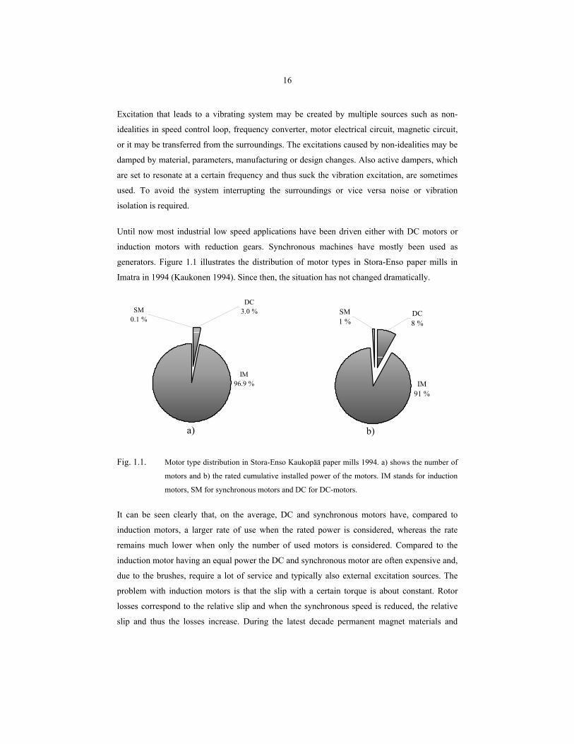
Until now most industrial low speed applications have been driven either with DC motors or
induction motors with reduction gears. Synchronous machines have mostly been used as
generators. Figure 1.1 illustrates the distribution of motor types in Stora-Enso paper mills in
Imatra in 1994 (Kaukonen 1994). Since then, the situation has not changed dramatically.
SM0.1 %
DC3.0 %
IM96.9 %
a)
IM91 %
DC8 %
SM1 %
b)
Fig. 1.1. Motor type distribution in Stora-Enso Kaukopää paper mills 1994. a) shows the number of
motors and b) the rated cumulative installed power of the motors. IM stands for induction
motors, SM for synchronous motors and DC for DC-motors.
It can be seen clearly that, on the average, DC and synchronous motors have, compared to
induction motors, a larger rate of use when the rated power is considered, whereas the rate
remains much lower when only the number of used motors is considered. Compared to the
induction motor having an equal power the DC and synchronous motor are often expensive and,
due to the brushes, require a lot of service and typically also external excitation sources. The
problem with induction motors is that the slip with a certain torque is about constant. Rotor
losses correspond to the relative slip and when the synchronous speed is reduced, the relative
slip and thus the losses increase. During the latest decade permanent magnet materials and
17
frequency control techniques have developed rapidly. This has brought that permanent magnet
synchronous machines have been used more widely and in different types of applications. With
permanent magnet synchronous machine gearless drives also the low speed area can be covered
maintaining high efficiency.
Permanent magnet synchronous machines (PMSMs) are nowadays used in several pilot
applications in paper mills. The machine type is also more and more often used in ship
propulsion systems and in direct driven windmills. Lift and hoist applications have pioneered
this development and successful mature products are already on the market.
New motor types are often developed for a certain application having certain boundary
conditions. There exist no design tradition and modern methods, such as the Finite Element
Method (FEM), are used to develop these new machine types.
1.1 Existing Calculation Methods
Traditionally, motors have been designed using analytical calculations, trial and error. The
analytical calculations, which formerly were done by hand, have been replaced by computer
aided analytical calculations in everyday design. Especially the system for induction motor
design has matured during the latest one hundred years. During the latest decades the FEM has
become a common tool to design and calculate electrical motors. The advantage of the method
is that it allows very accurate defining of the motor details and used materials, but also, at the
same time, focusing on the design of the most interesting areas or parameters. It also gives a lot
of possibilities to calculate different types of parameters such as torque, forces, electrical
parameters, material saturation level in different parts etc. Many commercial FEM-programs
are able to communicate with different types of calculation systems, like electrical circuit
simulators. This offers a lot of new possibilities to take into account different factors of
different systems and their mutual effect. Many programs also allow both steady state and
transient calculations.
Two-dimensional (2D) solvers have been available for about 20 years. Along the years the
development of the software as well as hardware has been enormous. In many cases the
problems were much too large or complex to be solved. Three-dimensional calculation has
become more popular, but the 2D FEM is still more commonly used. In some cases, 3D-
calculation doesn’t give any extra advantage since the calculation time or resources are
normally always limited. Also modelling is generally a lot easier with 2D. However, the
18
electrical motor has typical factors, which require 3D calculation to achieve accurate results.
These 3D-problems result from the rotor skewing, the motor end-effects in short machines or
the axial flux structure, which causes a changing of the factors along the radius. In permanent
magnet machines the magnet edges are often skewed in relation to the stator slots in order to
reduce the high cogging effect. This means that PMSMs, practically, almost always require 3D
calculation. Normally, it is not necessary to calculate and model the whole motor, but it is
enough to calculate only one sector of the machine because of its symmetry. When the flux
paths can be assumed to be on a plane, as in a radial flux motor with neglected coil end effects,
calculation can be made two-dimensionally in axial sections.
FEM includes large matrixes to be solved, and it is easy to understand, that large systems or
complex structures need a high amount of elements. The denser part of small elements can be
set in critical areas, like air-gap, to be examined, and a sparser element net in less meaningful
areas of the magnetic circuit. Transient or steady state rotating motor calculations still need a lot
of time for modelling and calculating. The process to model and calculate one single case in one
operational point may take days or even weeks. Often, this is a far too slow process, especially,
if the design obtained after the first cycle is not satisfying, but requires one or more iterations in
the process. This explains why there still exists a real need for a tool that makes modelling
faster, even though the results obtained would be to some extent less accurate.
Vibration problems in electrically driven mechanical systems are the sum of different factors. It
is not enough to model just the motor, drive or actuator. The mutual effects of different
components have a great impact on the final result. Until now, there exist various solution
methods and software to be applied to the respective mechanical systems and to the respective
drives and motors. It would be a huge if not an impossible task to combine the commercial
mechanics simulator, electrical motor FEM and circuit simulator with the system feedback.
Even if that could be done, the solution environment would grow so large and slow, that the
result would be a solver that cannot be applied for example to the R&D development process
where typically a number of iteration loops is needed.
1.2 Mechanical System Vibrations
Mechanical vibration is the sum of all sinusoidal movements of the system components. The
movements are not necessarily homogenous inside each of the components, but may also cause
internal forces. In its simplest form it may consist of only one frequency and amplitude, but in
multiplex systems it may include an infinite number of frequencies and amplitudes. In addition
19
to this, the vibrations may appear in different degrees of freedom. They may be components in
3D-coordinates or they can be radial or torsional (tangential). (Newland, 1989)
Each mechanical system has its own natural frequencies. This means that the shape and
materials give the system its properties to dampen excitations with different frequencies. These
properties in different degrees of freedom normally differ from each other. The more complex
the system is the higher is the number of natural frequencies. For example high-speed drives are
normally tried to be kept subcritical. In practice, this means that the rotational speed is kept
under the first bending mode of the rotating system. When this speed is exceeded, the rotor
starts to bend causing vibrations and great stress to the bearings. In addition to the shape and
material, the amplitude is in such a case also dependent of the rotational balance of the system
and thus high-speed systems are normally carefully balanced.
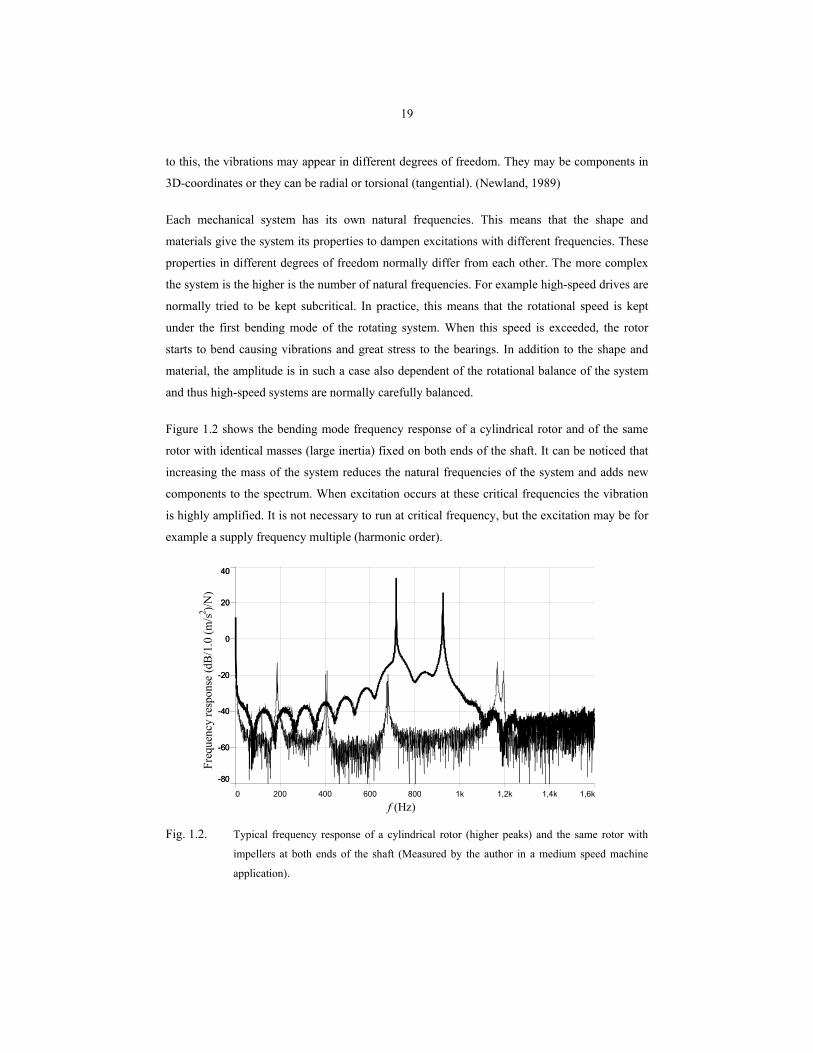
Figure 1.2 shows the bending mode frequency response of a cylindrical rotor and of the same
rotor with identical masses (large inertia) fixed on both ends of the shaft. It can be noticed that
increasing the mass of the system reduces the natural frequencies of the system and adds new
components to the spectrum. When excitation occurs at these critical frequencies the vibration
is highly amplified. It is not necessary to run at critical frequency, but the excitation may be for
example a supply frequency multiple (harmonic order).
0 200 400 600 800 1k 1,2k 1,4k 1,6k
-80
-60
-40
-20
0
20
40
[Hz]0 200 400 600 800 1k 1,2k 1,4k 1,6k
-80
-60
-40
-20
0
20
40
f (Hz)
Freq
uenc
y re
spon
se (d
B/1
.0 (m
/s )/
N)
2
Fig. 1.2. Typical frequency response of a cylindrical rotor (higher peaks) and the same rotor with
impellers at both ends of the shaft (Measured by the author in a medium speed machine
application).
20
When there is only one frequency and direction it is usually easy to find a way to dampen the
vibration or even totally get rid of it. In complex systems, damping the vibrations usually
requires a number of different technologies and is a compromise that leads to an acceptable
result. Typical ways of avoiding vibration problems are: decreasing the excitation, using a
resonator to suck the critical excitation, changing the mechanical structure to keep the natural
frequencies above the excitations or limiting the operation of the application to uncritical
rotational speeds.
Frequency converters often have the feature due to which so-called predefined forbidden
frequencies are avoided. This property is typically used, when in normal operation or during
acceleration the natural frequencies have to be passed fast. In practice, this means that these
frequencies with a certain tolerance are passed quickly and continuous operation is kept either
above or below this area.
The increased computer capacity and sophisticated programs have enabled the development of
good tools to calculate the natural frequencies of a component or even of a complicated
mechanical system. For the existing systems these can be found by means of the modal
analysis. The modal analysis is normally commenced by giving a mechanical impulse to the
system using an impulse hammer. After this, the frequency response of the mechanical system
is measured. Also the mode type can be found with this system.
1.3 Permanent Magnet Synchronous Motor
Traditionally, separately excited synchronous machines (SM) have been used as generators and
high power motors, often with higher voltages. Even though the SM has an efficiency that can
easily be higher than that of the induction or DC-motor and has an adjustable power factor, it is
seldom used in other than large industrial or traction applications. Compared to the induction
motor it is more difficult to use for example in applications that require a frequently starting of
the motor. As the denomination indicates, the rotor rotation has to be synchronized to the
voltage supply in both the velocity and phase angle in order to achieve a successful start up. In
practice, this calls for the use of vector controlled inverters. When using an induction motor the
start up may be done by directly switching the machine on the network. Also scalar inverters or
soft starters may be used. Also the SM structure with wound rotor and slip rings make them
more expensive to manufacture.
21
Since high-energy permanent magnets were discovered and frequency converters with
synchronous motor applications entered the market, the use of synchronous motors has rapidly
increased. Especially in low speed applications, which traditionally have been driven with
induction motors and reduction gears, the gearless PMSM drive is now often an alternative for
replacement. Induction motors are not used without gears in low speed applications since in
direct drives the relatively high per unit slip increases the rotor losses remarkably.
1.3.1 Development and Features of Permanent Magnet Material
The development of permanent magnet material has been fast during the latest decades. First,
the materials were based on Cobalt -, Tungsten - and Chromium – iron alloys. – Aluminium –
Nickel - Cobalt alloys were discovered in the 1930s, but the developing of Samarium – Cobalt
in the 1960s and finally Neodymium – Iron – Boron based magnets in the late seventies made it
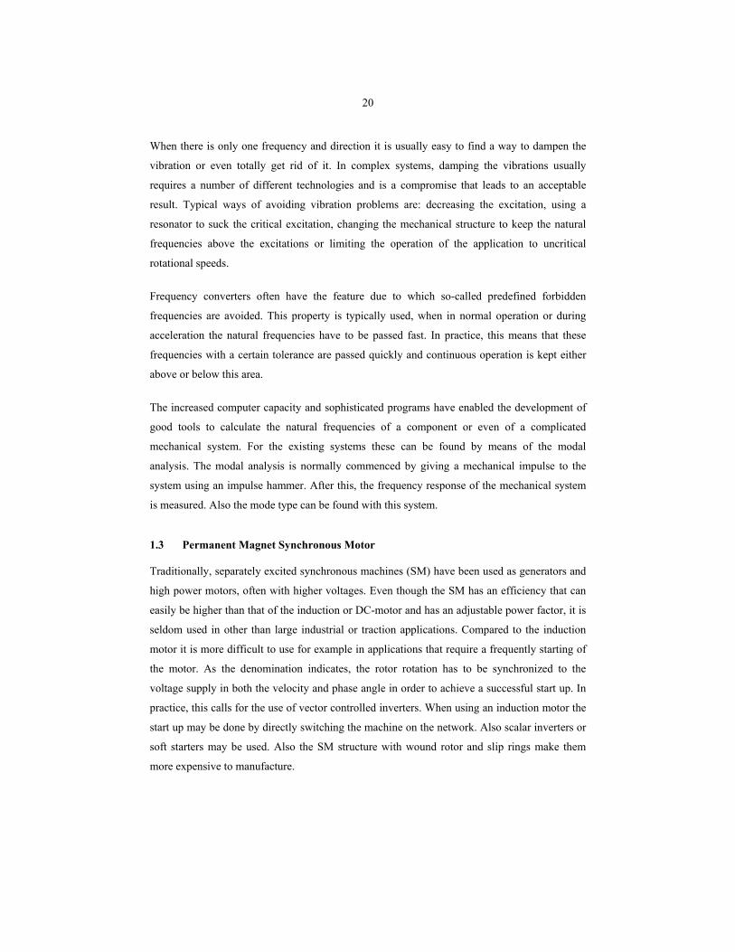
possible to benefit the permanent magnet materials in electrical motors. Figure 1.3 shows the
development of the energy content of different permanent magnet materials. The slope in the
curve is rather radical up to the year 1983. Since then, the energy density did not rise
dramatically nor any new types of material were published, but a lot of interest has been
focused on the material properties of Neo-magnets , like corrosion resistance and temperature
tolerance.
0
50
100
150
200
250
300
350
400
1910 1920 1930 1940 1950 1960 1970 1980 1990
Year
BHm
ax [
kJ/m
3 ]
Fig. 1.3. Development of the permanent magnet materials (Pyrhönen 1991).
22
Especially the good properties - a large remanence and coercivity - of SmCo and NdFeB
magnets have made it possible to introduce the application of these materials to industrial
motors. The coercive forces of both of these materials are large enough to tolerate a large
demagnetising armature reaction. This property makes the utilization of these materials possible
in motor and generator drives where negative d-axis currents are allowed. The traditional id = 0
control method is no more needed and new, much more effective control methods like DTC
(Direct Torque Control) have been introduced for application to PMSM drives (Luukko 2000).
Compared to motors driven with id = 0 control, the DTC control method offers the possibility
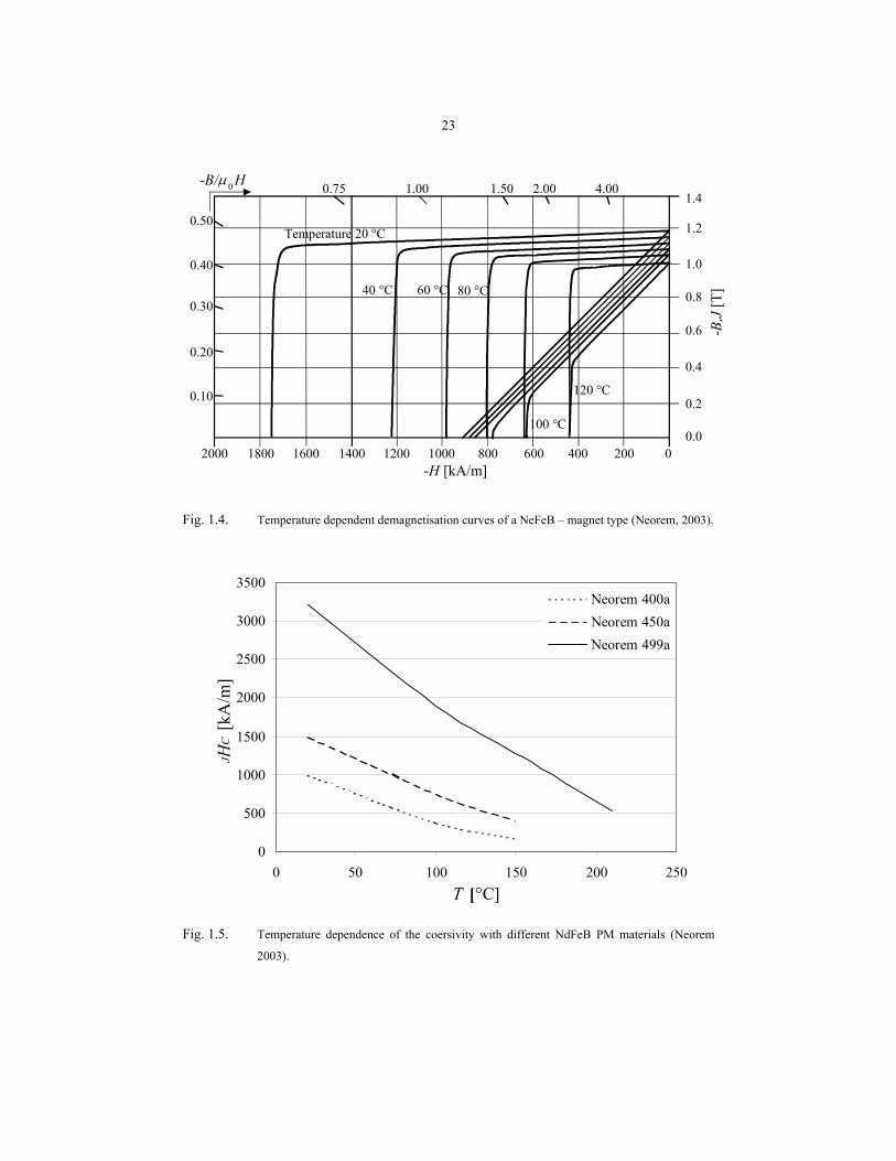
even to reduce the motor size. Figure 1.4 illustrates a typical NeFeB –type of permanent magnet
temperature dependent BH-curves. When the external opposite field strength becomes larger
then the so-called knee in the relevant curve, irreversible changes occur in the magnetisation.
This phenomenon is called demagnetisation.
However, there are some properties related to the use of permanent magnet materials , which
have slowed down the final break through. The patents concerning the materials and the
material prices have kept the cost of the magnets quite high. Also the manufacturing process is
quite complicated.
The first generation of NdFeB-magnets was susceptible to corrosion and had thus to be
protected carefully against humidity. Now, the materials have improved remarkably, but still
this weakness should be taken carefully into consideration. The phenomenon called white
corrosion emerges, when the magnetic material is exposed to hydrogen. When corrosion occurs,
the material turns to white powder and looses its properties. For this reason, practically all
magnetic materials are either coated or phosphated.
Typically, the temperature limitation for permanent magnets is below 120 degrees Celsius due
to the temperature dependent demagnetisation curves of the magnets. In the latest years, with
the use of special alloys this limit could be raised for some magnets to about 180 °C.
23
1.4
1.2
1.0
0.8
0.6
0.4
0.2
0.0
4.002.001.501.000.75
0.50
0.40
0.30
0.20
0.10
2000 1800 1600 1400 1200 1000 800 600 400 200 0
Temperature 20 °C
40 °C 60 °C 80 °C
100 °C
120 °C
-B/µ H0
-H [kA/m]
-B,J
[T]
Fig. 1.4. Temperature dependent demagnetisation curves of a NeFeB – magnet type (Neorem, 2003).
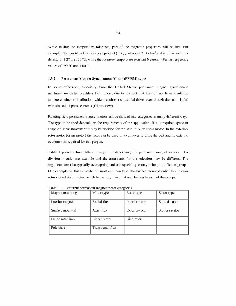
0
500
1000
1500
2000
2500
3000
3500
0 50 100 150 200 250T [°C]
J HC
[kA
/m]
Neorem 400aNeorem 450aNeorem 499a
Fig. 1.5. Temperature dependence of the coersivity with different NdFeB PM materials (Neorem
2003).
24
While raising the temperature tolerance, part of the magnetic properties will be lost. For
example, Neorem 400a has an energy product (BHmax) of about 310 kJ/m3 and a remanence flux
density of 1.28 T at 20 °C, while the lot more temperature resistant Neorem 499a has respective
values of 190 °C and 1.00 T.
1.3.2 Permanent Magnet Synchronous Motor (PMSM) types
In some references, especially from the United States, permanent magnet synchronous
machines are called brushless DC motors, due to the fact that they do not have a rotating
ampere-conductor distribution, which requires a sinusoidal drive, even though the stator is fed
with sinusoidal phase currents (Gieras 1999).
Rotating field permanent magnet motors can be divided into categories in many different ways.
The type to be used depends on the requirements of the application. If it is required space or
shape or linear movement it may be decided for the axial flux or linear motor. In the exterior-
rotor motor (drum motor) the rotor can be used in a conveyer to drive the belt and no external
equipment is required for this purpose.
Table 1 presents four different ways of categorizing the permanent magnet motors. This
division is only one example and the arguments for the selection may be different. The
arguments are also typically overlapping and one special type may belong to different groups.
One example for this is maybe the most common type: the surface mounted radial flux interior
rotor slotted stator motor, which has an argument that may belong to each of the groups.
Table 1.1. Different permanent magnet motor categories. Magnet mounting Motor type Rotor type Stator type
Interior magnet Radial flux Interior-rotor Slotted stator
Surface mounted Axial flux Exterior-rotor Slotless stator
Inside rotor iron Linear motor Disc-rotor
Pole shoe Transversal flux
25
Radial Flux Machine
The most typical or traditional electrical motor type is radial. In this type a cylindrical rotor
rotates inside a stator tube (interior-rotor motors) or, in some cases, a tube rotor rotates around a
stator (exterior-rotor motors). The motor properties, such as air-gap flux density distribution,
effective amount of permanent magnet material, cogging torque are, among other factors,
dependent on the magnet mounting, shape and volume. Also the manufacturing costs for the
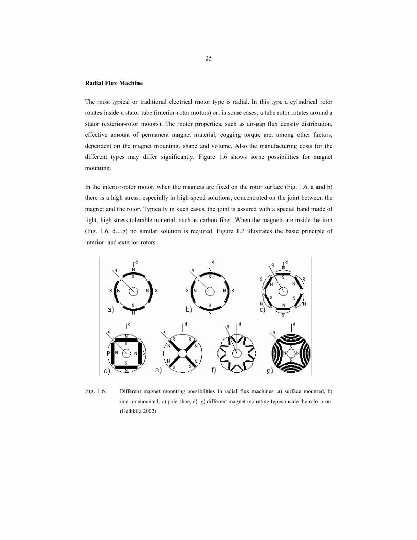
different types may differ significantly. Figure 1.6 shows some possibilities for magnet
mounting.
In the interior-rotor motor, when the magnets are fixed on the rotor surface (Fig. 1.6, a and b)
there is a high stress, especially in high-speed solutions, concentrated on the joint between the
magnet and the rotor. Typically in such cases, the joint is assured with a special band made of
light, high stress tolerable material, such as carbon fiber. When the magnets are inside the iron
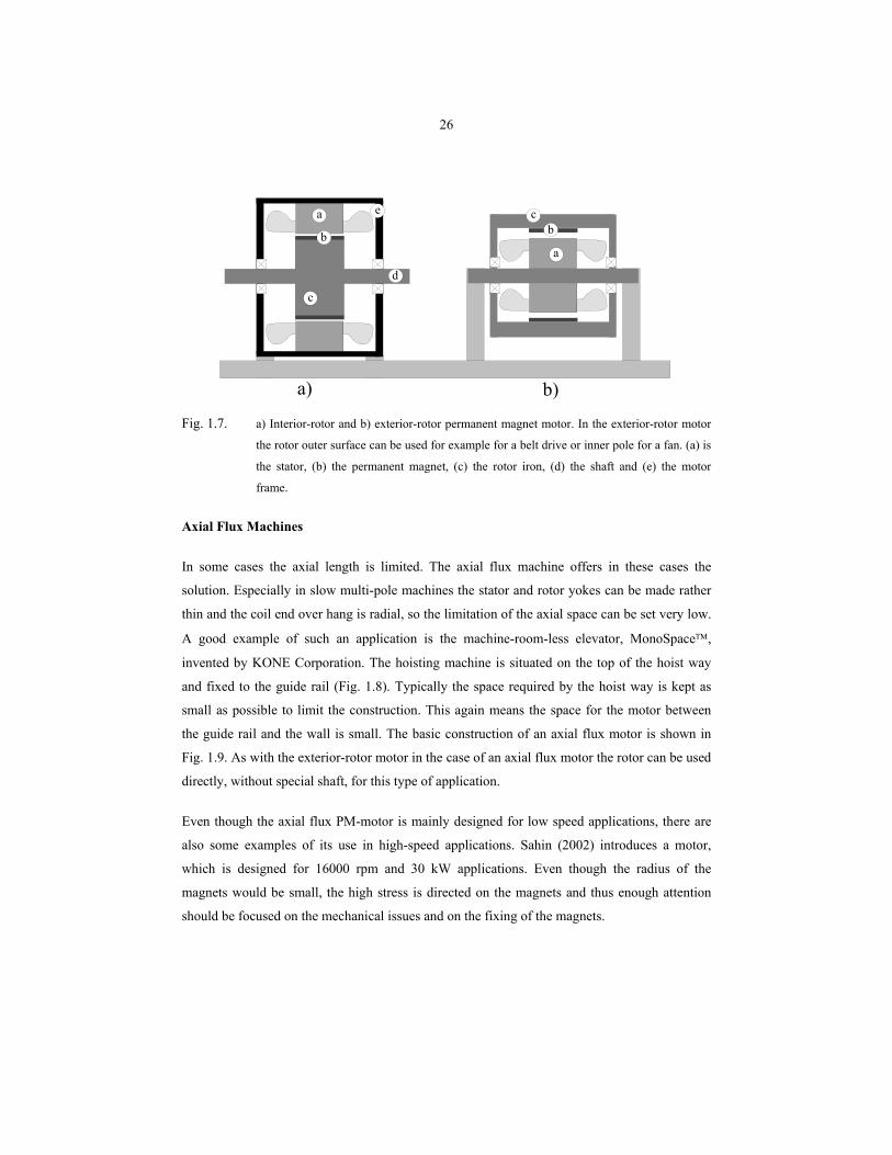
(Fig. 1.6, d…g) no similar solution is required. Figure 1.7 illustrates the basic principle of
interior- and exterior-rotors.
Fig. 1.6. Different magnet mounting possibilities in radial flux machines. a) surface mounted, b)
interior mounted, c) pole shoe, d)..g) different magnet mounting types inside the rotor iron.
(Heikkilä 2002)
26
c
c
a
a
b b
d
e
a) b)
Fig. 1.7. a) Interior-rotor and b) exterior-rotor permanent magnet motor. In the exterior-rotor motor
the rotor outer surface can be used for example for a belt drive or inner pole for a fan. (a) is
the stator, (b) the permanent magnet, (c) the rotor iron, (d) the shaft and (e) the motor
frame.
Axial Flux Machines
In some cases the axial length is limited. The axial flux machine offers in these cases the
solution. Especially in slow multi-pole machines the stator and rotor yokes can be made rather
thin and the coil end over hang is radial, so the limitation of the axial space can be set very low.
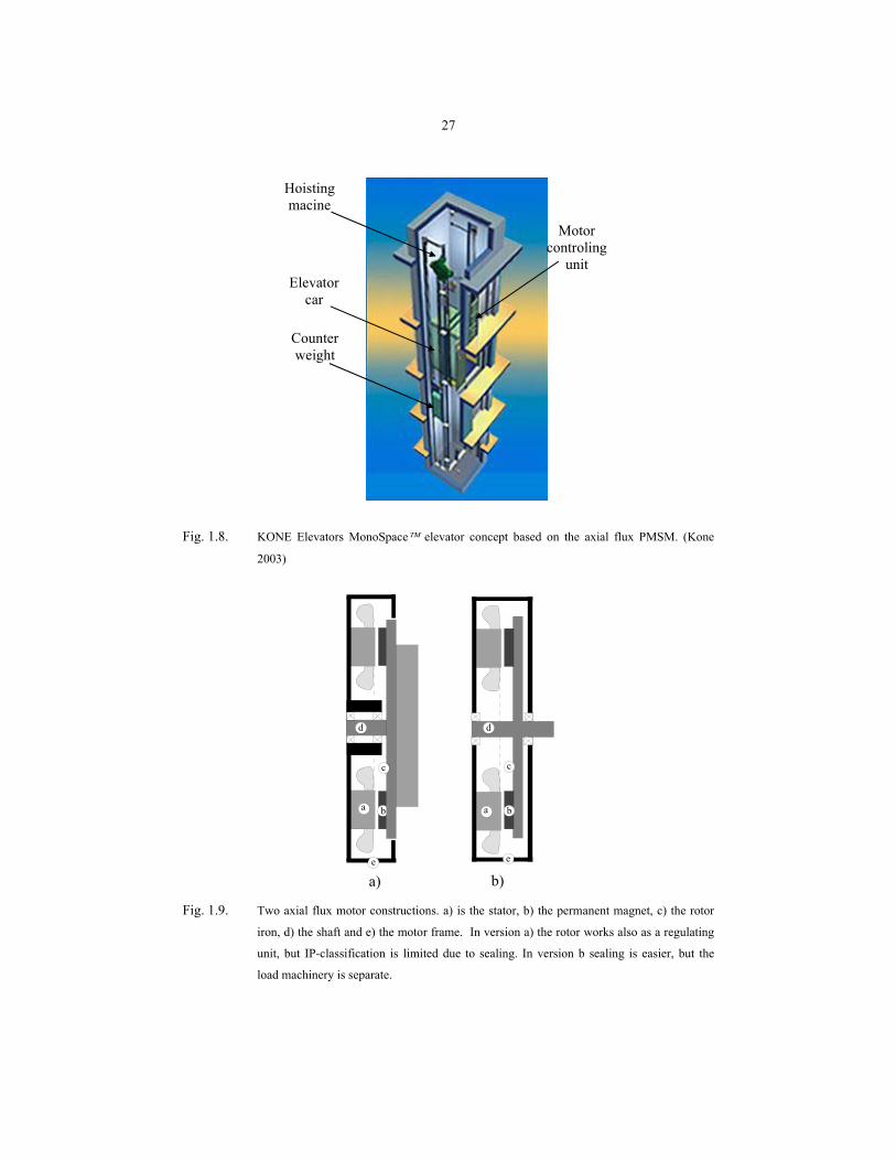
A good example of such an application is the machine-room-less elevator, MonoSpace,
invented by KONE Corporation. The hoisting machine is situated on the top of the hoist way
and fixed to the guide rail (Fig. 1.8). Typically the space required by the hoist way is kept as
small as possible to limit the construction. This again means the space for the motor between
the guide rail and the wall is small. The basic construction of an axial flux motor is shown in
Fig. 1.9. As with the exterior-rotor motor in the case of an axial flux motor the rotor can be used
directly, without special shaft, for this type of application.
Even though the axial flux PM-motor is mainly designed for low speed applications, there are
also some examples of its use in high-speed applications. Sahin (2002) introduces a motor,
which is designed for 16000 rpm and 30 kW applications. Even though the radius of the
magnets would be small, the high stress is directed on the magnets and thus enough attention
should be focused on the mechanical issues and on the fixing of the magnets.
27
Hoistingmacine
Motor controling
unitElevator
car
Counterweight
Fig. 1.8. KONE Elevators MonoSpace elevator concept based on the axial flux PMSM. (Kone
2003)
a
c
d
e
a b
c
d
e
c
b
a) b)
Fig. 1.9. Two axial flux motor constructions. a) is the stator, b) the permanent magnet, c) the rotor
iron, d) the shaft and e) the motor frame. In version a) the rotor works also as a regulating
unit, but IP-classification is limited due to sealing. In version b sealing is easier, but the
load machinery is separate.
28
In certain applications the axial flux motor requires less material than the radial motor does for
the same operation. In their study Sitapati and Krishnan (2001), compared one radial and four
axial field topologies. Their conclusion was that the axial flux motor has a higher power density
compared to radial flux motor. Zhang et al. (1996) came to the same conclusion concerning the
torque density, when the reference considered is the amount of active material.
Transversal Flux Machines
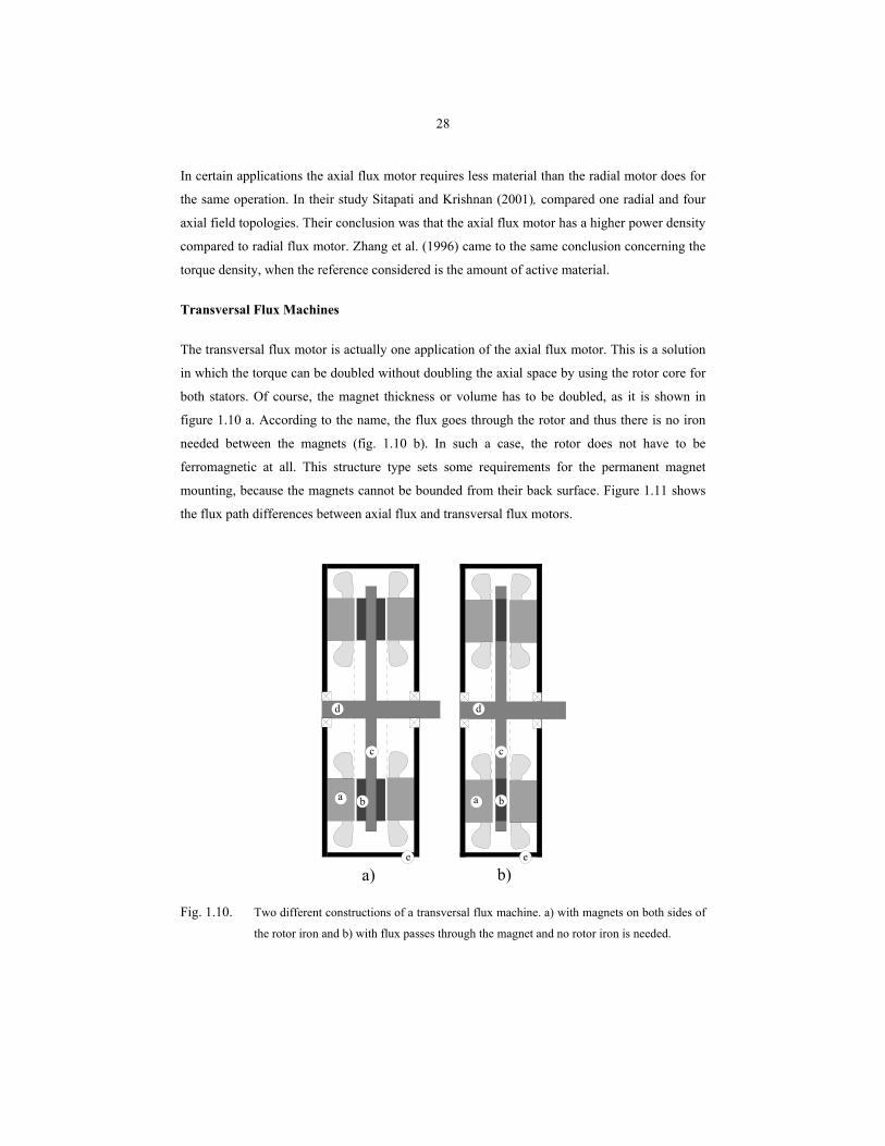
The transversal flux motor is actually one application of the axial flux motor. This is a solution
in which the torque can be doubled without doubling the axial space by using the rotor core for
both stators. Of course, the magnet thickness or volume has to be doubled, as it is shown in
figure 1.10 a. According to the name, the flux goes through the rotor and thus there is no iron
needed between the magnets (fig. 1.10 b). In such a case, the rotor does not have to be
ferromagnetic at all. This structure type sets some requirements for the permanent magnet
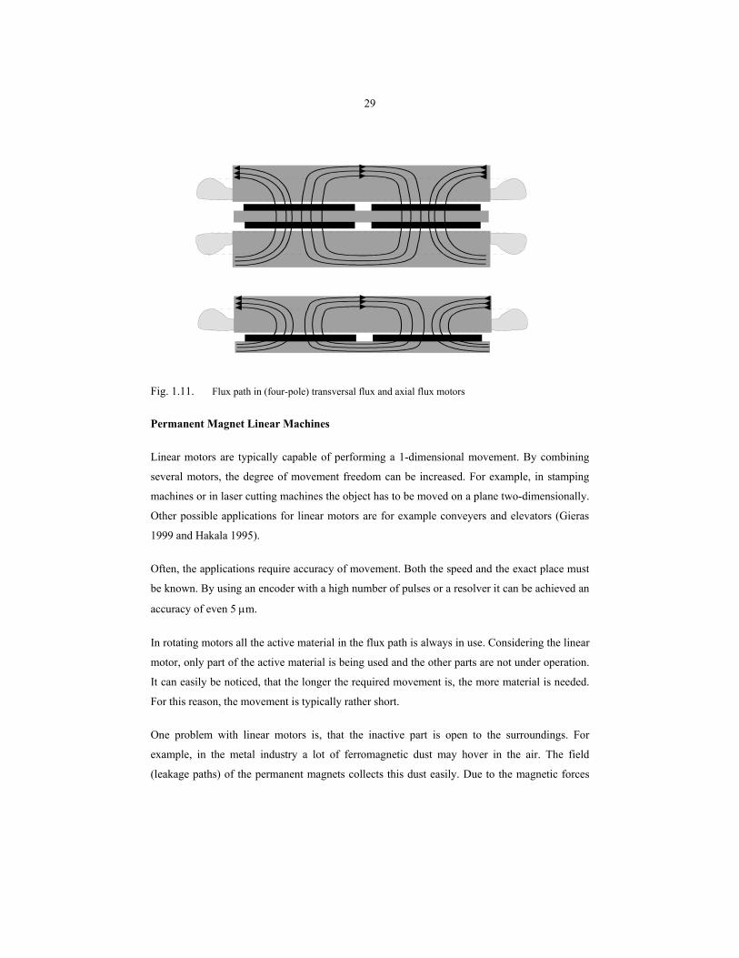
mounting, because the magnets cannot be bounded from their back surface. Figure 1.11 shows
the flux path differences between axial flux and transversal flux motors.
a b
c
d
e
a b
c
d
e
a) b)
Fig. 1.10. Two different constructions of a transversal flux machine. a) with magnets on both sides of
the rotor iron and b) with flux passes through the magnet and no rotor iron is needed.
29
Fig. 1.11. Flux path in (four-pole) transversal flux and axial flux motors
Permanent Magnet Linear Machines
Linear motors are typically capable of performing a 1-dimensional movement. By combining
several motors, the degree of movement freedom can be increased. For example, in stamping
machines or in laser cutting machines the object has to be moved on a plane two-dimensionally.
Other possible applications for linear motors are for example conveyers and elevators (Gieras
1999 and Hakala 1995).
Often, the applications require accuracy of movement. Both the speed and the exact place must
be known. By using an encoder with a high number of pulses or a resolver it can be achieved an
accuracy of even 5 µm.
In rotating motors all the active material in the flux path is always in use. Considering the linear
motor, only part of the active material is being used and the other parts are not under operation.
It can easily be noticed, that the longer the required movement is, the more material is needed.
For this reason, the movement is typically rather short.
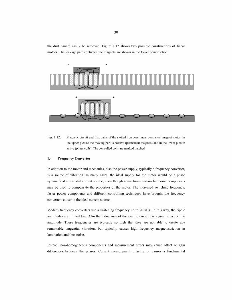
One problem with linear motors is, that the inactive part is open to the surroundings. For
example, in the metal industry a lot of ferromagnetic dust may hover in the air. The field
(leakage paths) of the permanent magnets collects this dust easily. Due to the magnetic forces
30
the dust cannot easily be removed. Figure 1.12 shows two possible constructions of linear
motors. The leakage paths between the magnets are shown in the lower construction.
Fig. 1.12. Magnetic circuit and flux paths of the slotted iron core linear permanent magnet motor. In
the upper picture the moving part is passive (permanent magnets) and in the lower picture
active (phase coils). The controlled coils are marked hatched.
1.4 Frequency Converter
In addition to the motor and mechanics, also the power supply, typically a frequency converter,
is a source of vibration. In many cases, the ideal supply for the motor would be a phase
symmetrical sinusoidal current source, even though some times certain harmonic components
may be used to compensate the properties of the motor. The increased switching frequency,
faster power components and different controlling techniques have brought the frequency
converters closer to the ideal current source.
Modern frequency converters use a switching frequency up to 20 kHz. In this way, the ripple
amplitudes are limited low. Also the inductance of the electric circuit has a great effect on the
amplitude. These frequencies are typically so high that they are not able to create any
remarkable tangential vibration, but typically causes high frequency magnetostriction in
lamination and thus noise.
Instead, non-homogeneous components and measurement errors may cause offset or gain
differences between the phases. Current measurement offset error causes a fundamental
31
harmonic component and current measurement gain error causes a second order harmonic
component to the torque (Chung 1998, Laurila 2002).
1.5 Outline of the Thesis
The behaviour of PM-motors has been studied widely during the latest years. Different methods
of reducing the torque ripple have been developed and studied in many sources. Also
calculation methods to estimate the torque and cogging have been an interesting field of study.
Most of the studies are carried out with the finite element method, which gives reliable results
when modelling is done carefully, but requires a lot of work and calculation recourses. Analytic
methods are mainly used to calculate a certain factor in the motor model.
The critical frequencies in a mechanical system are difficult to predict. Traditionally, a
prototype is built by means of which practical results can be obtained. However, to avoid the
need to build expensive prototypes a project was founded to model the torque vibrations of a
mechanical application including the frequency converter, motor, actuator and the control
system. This study is part of that project.
The work has two objectives. 1) to create an analytical, reluctance network based and accurate
enough calculation method to evaluate the instantaneous electro-magnetic torque of PMSMs
with rotor surface mounted magnets. The calculation model must be applicable to the larger
mechanics simulation system mentioned above 2) to minimize the output torque ripple of the
prototype machine developed during the study.
Zhu et al. (1993 & 2000) have been widely referred in the area of permanent magnet motor
modeling and the cogging phenomenon. They developed analytic approach to flux density
created by the permanent magnets in the air-gap. Their approach is also one of the bases in this
study and is one the main requirements in order to handle the torque component analytically.
They also studied widely the effect of different design factors on the torque quality.
Due to the traditional structure of electric motors most of the articles handle radial flux
(cylindrical) motors. Most of the effects are about equal when compared with axial flux (AF)
motors, but there are also some differences. One these is the magnetization direction in radial
magnets (Jahns 1996). The other difference is that in radial motor the torque is created with
constant radius, when in AF motors it varies. The force created in the stator outer radius creates
32
higher torque than same force in the inner radius. This factor was not found in any of the used
references.
Li & Slemon (1988) were among the first to study the effects of NdFeB –magnet to torque
vibration in synchronous machines. As with many others their study was base on the 2-
dimensional approach, which limits the possibilities in magnet, slot and teeth widths. They
found optimum width for square magnet and slot/tooth width. Calculation was made with linear
stator (linear motor model). While the calculation programs developed Ishikawa & Slemon
(1993) continued on this basis but with cylindrical model, which also took the rotor curvature in
to account. The results they got where slightly different compared with the linear model.
However, a simple, but reliable enough tool to evaluate the effect of different factors on the
torque ripple was not found in the references. One limiting factor for this may be the demand of
three dimensional calculations due to the structure of the motor. It is aimed at developing a
calculation environment with analytical equations to solve radial and axial flux PMSMs with
rotor surface mounted permanent magnets simply and fast, but still sufficiently accurately. The
modelling of the motor and its different factors should be simple, but still the achieved results
must be useful and reliable. The model is to be fed with the currents, required mechanical
torque and speed and the output of the calculation is the torque created by the motor. If the
latter differs from the torque of the actuator, the difference either accelerates or decelerates the
system. Also the possibility to connect the model with other factors (power source, control
circuit and mechanics) that have a great impact to the torque and vibration would make this type
of model most interesting.
This difference (excitation) is generated by the non-idealities of the electric and magnetic
systems. How the mechanical system will react to this depends on the frequency of the
excitation and frequency response of the mechanical system.
The second chapter introduces the equations to create a calculation model for the surface
mounted rotating permanent magnet motor. This model may be applied to both the radial and
axial flux motor. The main interest is, however, focused in the latter, since the results may thus
be compared and verified with the results achieved with the testing prototype.
The third chapter discusses different factors that affect the vibration created by the motor. These
are factors that are related to material properties, geometry and asymmetry. In a brief review it
is also focused on the frequency converter non-idealities.
33
In the fourth chapter, the analytic calculations are compared with the FEM-calculations and
measured results. A conclusion of the research is given in the last chapter.
1.6 Scientific Contribution of The Work
The scientific contribution of the work can be summarized as follows:
1. Analytic equations and methods are introduced for the fast and reliable torque
calculation of a surface mounted axial flux permanent magnet machine and the
possibility is discussed to integrate the method as part of the total electro-mechanic
system calculation.
2. A close, theoretical study is done of the effects of different factors on the torque
quality.
3. A large number of measurements are performed to verify the calculation method.
Typically, the calculating of an axial flux permanent magnet machine is performed applying a
3D FEM-method, by means of which it is possible to take into account the radius and non-
uniform structure of the teeth and the other electrical and magnetic parts of the machine. The
calculation requires a lot of time and computer recourses. This study will prove that calculating
can also be done with analytical methods progressing the following way: first, the magnet is
divided into slices and the calculation is performed for each section separately, then, the parts
are submitted for final results. This method offers the advantage that a lot of time in design and
calculation can be saved.
The calculation method is used to study the effect of the different factors of the permanent
magnet and of the other parts of the magnetic circuit on the torque quality. It is proven with
different methods that combining in a suitable way the magnet shaping, magnetic circuit
asymmetry and magnetic circuit dimensioning it is possible to reduce the torque ripple to fulfil
the requirements of almost any electric motor application.
The measurements are carried out with a number of different permanent magnet shapes and
distributions as well as with some modifications made in the stator. Also the effect of supply
non-linearities is measured. These measurements are verified with different calculation methods
and thus support the reliability of this method.
34
2 TORQUE CALCULATION MODEL
This chapter introduces the analytical equations that create the basics of the calculation model
for rotating permanent magnet motors having the permanent magnet material attached on the
rotor surface. The model takes into account the stator magneto motive force harmonics, the air-
gap permeance harmonics and the rotor permanent magnet shapes. With some slight
modifications the model can be applied to both radial and axial flux motors. However, the main
interest is focused on the latter.
2.1 General
The Finite Element Method has become a common tool to design and calculate electrical
motors in steady state and in transients. Even though progress in the development of computer
technology and calculation programs has been rapid and computers have become faster and
capable of treating a large amount of data, the accurate modelling of the motors remains still a
time consuming process, especially if a three-dimensional solution is required. The increasing
demand on the motor performance calls for more reliable results, more accurate models and
shorter time steps in dynamic simulation. In radial flux motors two-dimensional (2D) modelling
is often accurate enough, especially if the motor is long and the end effects in the motor may be
ignored. As an example, in the case of slot skewing or special magnet shapes modelling must be
done in axial slices in order that the geometry should be taken into consideration. Three-
dimensional (3D) modelling has thus been increasingly approved, though the fact that - as it can
be assumed - with the accurate 3D model calculation and modelling require really a lot of time.
In axial flux machines many parameters change as a function of the rotor radius. Inherently, a
pure 3D modelling or 2D modelling using several slices is required if accurate torque quality
studies should be performed. The results given in chapter 4.2 confirm this statement. In some
occasions the average torque of an axial flux machine may, however, be calculated using the
simplified 2D model.
With an analytical model of the motor the calculation results obtained may be less accurate than
those obtained with FEM, but in many cases the required results can be reached in a fractional
time. Especially used as a normal design tool the analytical calculation program is very
attractive. In the project of the this research the motor calculation has to be part of a whole
electromechanical drive model and compatible with the calculation of the other parts. In such a
case FEM cannot be applied and thus an analytical model is needed.
35
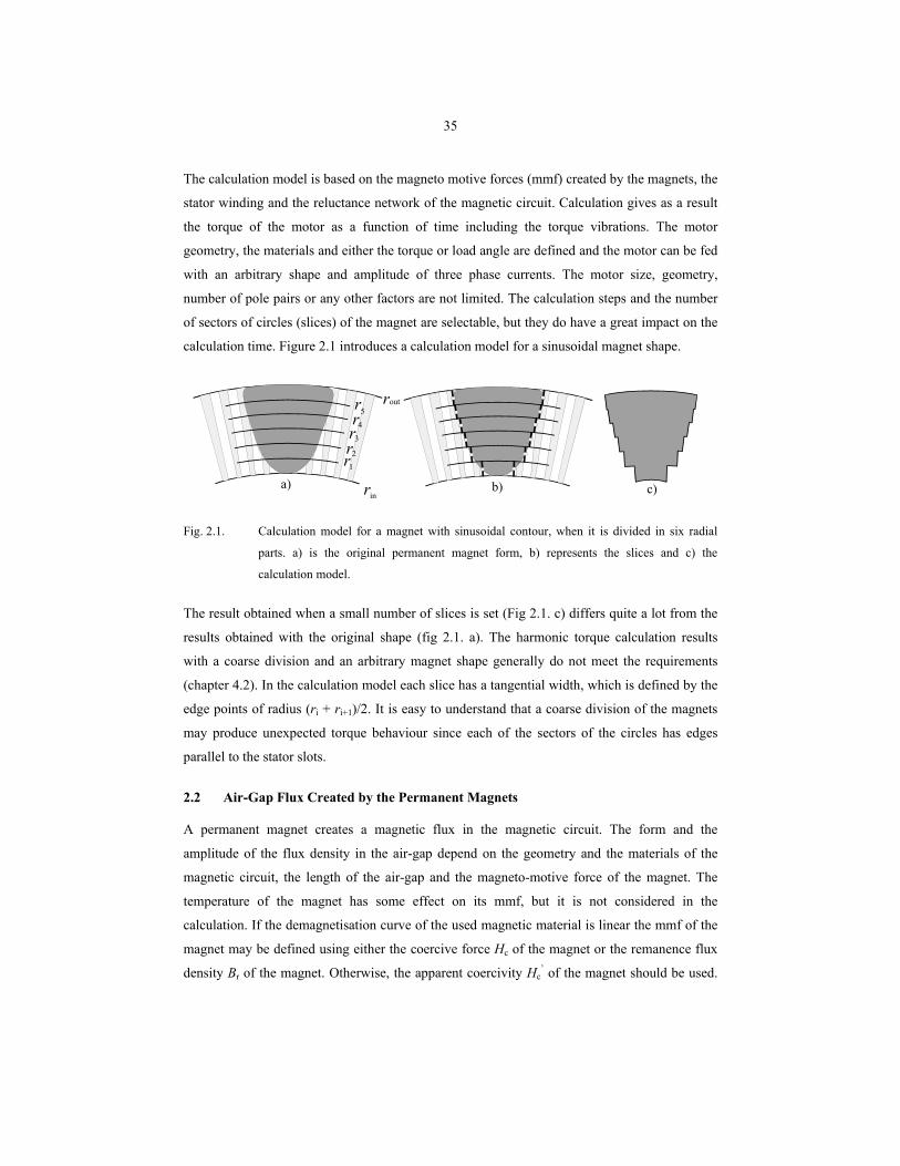
The calculation model is based on the magneto motive forces (mmf) created by the magnets, the
stator winding and the reluctance network of the magnetic circuit. Calculation gives as a result
the torque of the motor as a function of time including the torque vibrations. The motor
geometry, the materials and either the torque or load angle are defined and the motor can be fed
with an arbitrary shape and amplitude of three phase currents. The motor size, geometry,
number of pole pairs or any other factors are not limited. The calculation steps and the number
of sectors of circles (slices) of the magnet are selectable, but they do have a great impact on the
calculation time. Figure 2.1 introduces a calculation model for a sinusoidal magnet shape.
in
12
3
45
outr r
r
rrrr
a) b) c)
Fig. 2.1. Calculation model for a magnet with sinusoidal contour, when it is divided in six radial
parts. a) is the original permanent magnet form, b) represents the slices and c) the
calculation model.
The result obtained when a small number of slices is set (Fig 2.1. c) differs quite a lot from the
results obtained with the original shape (fig 2.1. a). The harmonic torque calculation results
with a coarse division and an arbitrary magnet shape generally do not meet the requirements
(chapter 4.2). In the calculation model each slice has a tangential width, which is defined by the
edge points of radius (ri + ri+1)/2. It is easy to understand that a coarse division of the magnets
may produce unexpected torque behaviour since each of the sectors of the circles has edges
parallel to the stator slots.
2.2 Air-Gap Flux Created by the Permanent Magnets
A permanent magnet creates a magnetic flux in the magnetic circuit. The form and the
amplitude of the flux density in the air-gap depend on the geometry and the materials of the
magnetic circuit, the length of the air-gap and the magneto-motive force of the magnet. The
temperature of the magnet has some effect on its mmf, but it is not considered in the
calculation. If the demagnetisation curve of the used magnetic material is linear the mmf of the
magnet may be defined using either the coercive force Hc of the magnet or the remanence flux
density Br of the magnet. Otherwise, the apparent coercivity Hc’ of the magnet should be used.
36
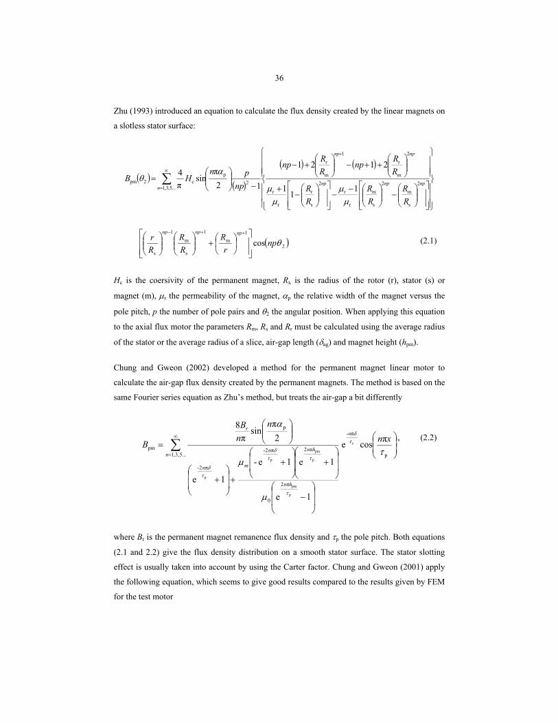
Zhu (1993) introduced an equation to calculate the flux density created by the linear magnets on
a slotless stator surface:
( )( )
( ) ( )∑∞
=
+
−
−−
−
+
++−
+−
−
=
...5,3,12
s
m
2
s
m
r
r
2
s
r
r
r
2
m
r1
m
r
2p
c2pm1
11
2121
12π
sinπ4
nnpnpnp
npnp
RR
RR
RR
RR
npRR
np
nppn
HB
µµ
µµ
αθ
( )2
1m
1
s
m
1
s
cos θnpr
RRR
Rr npnpnp
+
++−
(2.1)
Hc is the coersivity of the permanent magnet, Rx is the radius of the rotor (r), stator (s) or
magnet (m), µr the permeability of the magnet, αp the relative width of the magnet versus the
pole pitch, p the number of pole pairs and θ2 the angular position. When applying this equation
to the axial flux motor the parameters Rm, Rs and Rr must be calculated using the average radius
of the stator or the average radius of a slice, air-gap length (δag) and magnet height (hpm).
Chung and Gweon (2002) developed a method for the permanent magnet linear motor to
calculate the air-gap flux density created by the permanent magnets. The method is based on the
same Fourier series equation as Zhu’s method, but treats the air-gap a bit differently
−
+
+
+
+
= ∑∞
= p
π-
...5,3,1
π2
0
π2π2-
π2-
pr
pmπcose
1e
1e1e-
1e
2π
sinπ
8
s
p
pm
p
pm
p
p
τ
µ
µ
α
τδ
τ
ττδ
τδ
xnn
nB
Bn
n
hn
hnn
mn
, (2.2)
where Br is the permanent magnet remanence flux density and τp the pole pitch. Both equations
(2.1 and 2.2) give the flux density distribution on a smooth stator surface. The stator slotting
effect is usually taken into account by using the Carter factor. Chung and Gweon (2001) apply
the following equation, which seems to give good results compared to the results given by FEM
for the test motor
37
′+
′+−=
gwgwk so
ss
so
4π1ln
π41c ττ
, (2.3)
where τs is the slot pitch, wso the width of the slot opening and g’ the total air-gap length.
However, in this case, it is not sufficient to use only the Cater factor; the permeance function of
the air gap region is required. Several sources discuss different methods to calculate the
permeance function kΛ. Heller and Hamata (1977) present different equations, depending on the
air-gap length, slot and slot opening parameters. The following equation introduced by Weber
(1928) is one of the most appropriate equations referred to by Heller and Hamata. The air-gap
flux density along a slot pitch is modified by the permeance function
( ) maxd
2max
πsin21 BBkB n
−== Λ α
αβα , (2.4)
where
so
so
ww
n s −=
τ. (2.5)
β is a function of wso/δ and αd is the angle corresponding to slot pitch. The depth of the drop in
the flux density under the slot opening depends on the distance to the stator surface, where the
distribution is calculated.
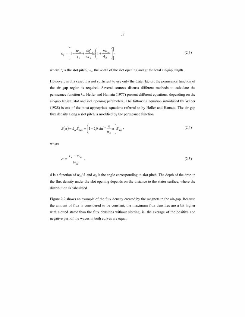
Figure 2.2 shows an example of the flux density created by the magnets in the air-gap. Because
the amount of flux is considered to be constant, the maximum flux densities are a bit higher
with slotted stator than the flux densities without slotting, ie. the average of the positive and
negative part of the waves in both curves are equal.
38
-1-0.8-0.6-0.4-0.2
00.20.40.60.8
1
B [T
]
Bpm
Bpm slottedstator
Fig. 2.2. Air-gap flux density along one pole pair area created by the permanent magnet, with and
without slotting
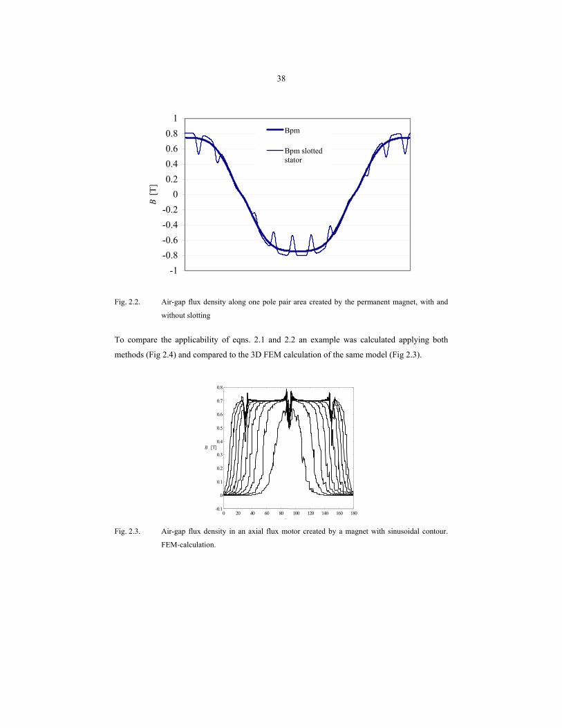
To compare the applicability of eqns. 2.1 and 2.2 an example was calculated applying both
methods (Fig 2.4) and compared to the 3D FEM calculation of the same model (Fig 2.3).
0 20 40 60 80 100 120 140 160 180-0.1
0 0.1 0.2 0.3 0.4 0.5 0.6 0.7 0.8
α
B [T]
Fig. 2.3. Air-gap flux density in an axial flux motor created by a magnet with sinusoidal contour.
FEM-calculation.
39
-0.10
0.10.20.30.40.50.60.70.8
0 30 60 90 120 150 180(°)
B [T
]
-0.10
0.10.20.30.40.50.60.70.8
0 30 60 90 120 150 180(°)
B [T
]
a) b)
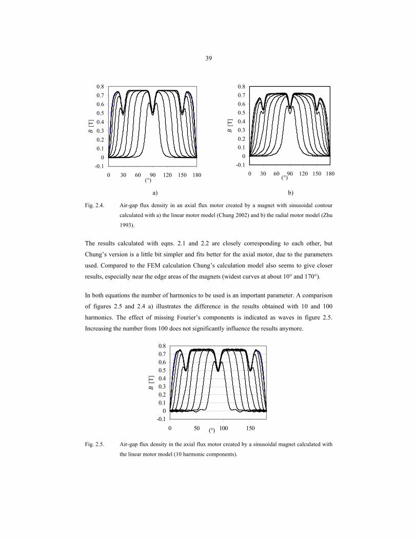
Fig. 2.4. Air-gap flux density in an axial flux motor created by a magnet with sinusoidal contour
calculated with a) the linear motor model (Chung 2002) and b) the radial motor model (Zhu
1993).
The results calculated with eqns. 2.1 and 2.2 are closely corresponding to each other, but
Chung’s version is a little bit simpler and fits better for the axial motor, due to the parameters
used. Compared to the FEM calculation Chung’s calculation model also seems to give closer
results, especially near the edge areas of the magnets (widest curves at about 10° and 170°).
In both equations the number of harmonics to be used is an important parameter. A comparison
of figures 2.5 and 2.4 a) illustrates the difference in the results obtained with 10 and 100
harmonics. The effect of missing Fourier’s components is indicated as waves in figure 2.5.
Increasing the number from 100 does not significantly influence the results anymore.
-0.10
0.10.20.30.40.50.60.70.8
0 50 100 150(°)
B [T
]
Fig. 2.5. Air-gap flux density in the axial flux motor created by a sinusoidal magnet calculated with
the linear motor model (10 harmonic components).
40
The calculation is simple and fast if the shape of the magnet is a square and has no skew related
to the stator slots. When the shape of the magnets is more complicated the calculation has to be
done in several slices. The bigger the amount of slices the more accurate is the result. A coarse
division of the sector into slices may cause unexpected torque vibrations since the width of an
individual slice may appear to be seriously disadvantageous with reference to the pole pitch or
slot pitch.
2.3 Magnetic Circuit
The magnetic circuit of the motor, consisting of the stator iron, rotor iron, air-gap, magnet and
slot, is modelled in the model developed with a reluctance network, which takes the saturation
of the iron into account. This means that several iteration circles, in which the permeability in
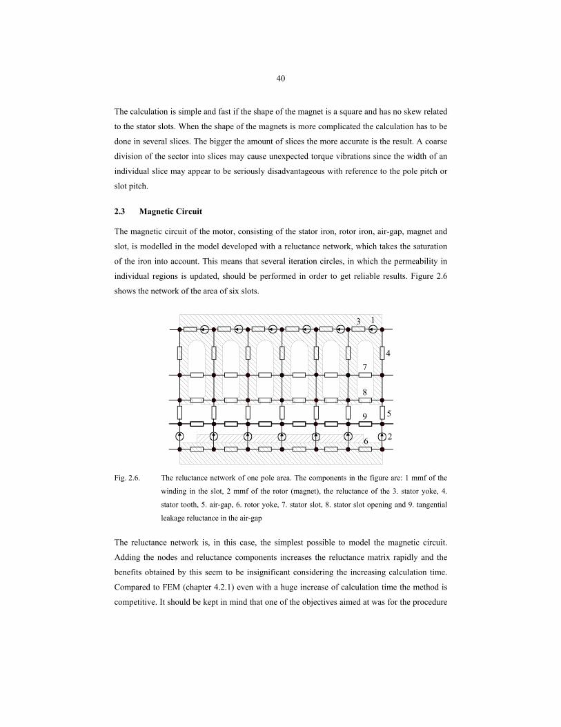
individual regions is updated, should be performed in order to get reliable results. Figure 2.6
shows the network of the area of six slots.
4
3
7
1
8
59
26
Fig. 2.6. The reluctance network of one pole area. The components in the figure are: 1 mmf of the
winding in the slot, 2 mmf of the rotor (magnet), the reluctance of the 3. stator yoke, 4.
stator tooth, 5. air-gap, 6. rotor yoke, 7. stator slot, 8. stator slot opening and 9. tangential
leakage reluctance in the air-gap
The reluctance network is, in this case, the simplest possible to model the magnetic circuit.
Adding the nodes and reluctance components increases the reluctance matrix rapidly and the
benefits obtained by this seem to be insignificant considering the increasing calculation time.
Compared to FEM (chapter 4.2.1) even with a huge increase of calculation time the method is
competitive. It should be kept in mind that one of the objectives aimed at was for the procedure
41
to be part of system calculation. In such a case, it is not appropriate to enlarge the matrix sizes
and increase the calculation time. Also the results given in chapter four prove this simple
network to be accurate. The calculation procedure itself does not limit the network size.
In case of an integer slot winding the total calculation model is made for one pole pair of the
machine, and this one pole pair module is connected from both ends to each other to take the
flux passing edge of the model in to consideration. This means that the model analyses the
machine calculating just one pole pair. However, this is not enough in the case of a fractional
slot winding or in cases in which non-uniformity in the magnet positions or magnet sizes is
included. In these cases several pole pairs must be calculated. The total torque is reached by
multiplying the torque of the calculated area with the number of similar areas.
The main route of the flux goes along the stator yoke, the teeth, the air-gap and the rotor yoke.
The BH-curve of the magnetic material is defined, and the values of the reluctances are
calculated depending on the saturation of the magnetic circuit components. The permeability of
air is constant, and the air-gap reluctance as well as the leakage reluctances are thus kept
constant.
According to the calculations made with this procedure, the tangential leakage reluctance has a
very small effect on the calculation results, but it adds one calculation circuit in each tooth area.
When calculating asymmetric cases as e.g. an additional slot in the stator (described closer in
chapter 3), a model of the whole motor including all pole pairs is needed. If in such asymmetric
cases this component is neglected the size of the matrixes and calculation time will be
considerably reduced. The flux φ in each circuit is solved by
[ ] [ ] [ ]NIR 1−=φ , (2.6)
where [R] is the reluctance matrix and [NI] is mmf matrix.
Reluctance networks have been successfully used also with other types of electrical motors.
Perho (2002) presented a method to calculate induction motors with the reluctance model..
However, Perho defines the circuit using an amount of elements that is much larger compared
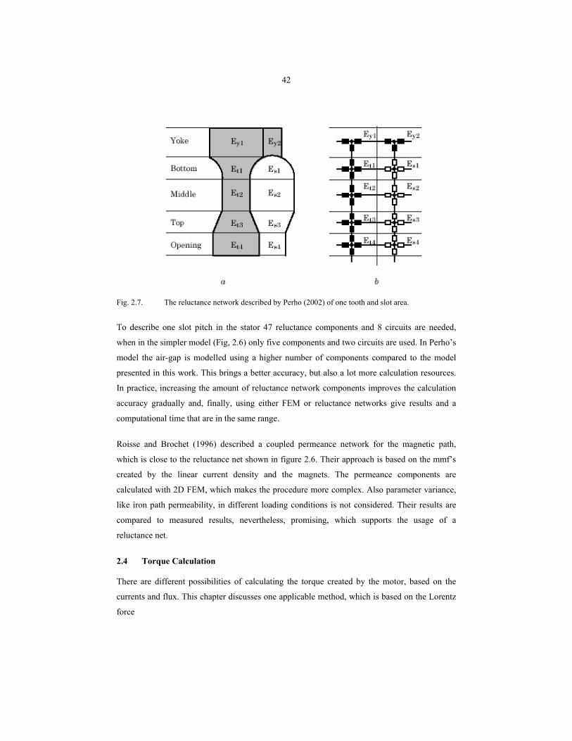
to the model introduced in this work. Figure 2.7 shows the reluctance model of one slot and
tooth area as it is described Perho’s work.
42
Fig. 2.7. The reluctance network described by Perho (2002) of one tooth and slot area.
To describe one slot pitch in the stator 47 reluctance components and 8 circuits are needed,
when in the simpler model (Fig, 2.6) only five components and two circuits are used. In Perho’s
model the air-gap is modelled using a higher number of components compared to the model
presented in this work. This brings a better accuracy, but also a lot more calculation resources.
In practice, increasing the amount of reluctance network components improves the calculation
accuracy gradually and, finally, using either FEM or reluctance networks give results and a
computational time that are in the same range.
Roisse and Brochet (1996) described a coupled permeance network for the magnetic path,
which is close to the reluctance net shown in figure 2.6. Their approach is based on the mmf’s
created by the linear current density and the magnets. The permeance components are
calculated with 2D FEM, which makes the procedure more complex. Also parameter variance,
like iron path permeability, in different loading conditions is not considered. Their results are
compared to measured results, nevertheless, promising, which supports the usage of a
reluctance net.
2.4 Torque Calculation
There are different possibilities of calculating the torque created by the motor, based on the
currents and flux. This chapter discusses one applicable method, which is based on the Lorentz
force
43
)( BvEdQFdrrrr
×+= , (2.7)
In practice, the sum of the tangential components created by the electric field strength ( Er
) is
zero and, thus, does not create any torque. This is due to the fact that the electrical field around
the slot is equal to the opposite directions thus compensating each other. Here, only the last
component in bracket part of equation 2.7 is considered.
)()( BlddIBvdQFdrrrrr
×=×= (2.8)
The Maxwell stress tensor is also often used in the torque calculation. In practice, the Maxwell
stress tensor may be calculated only by using FEM. The normal and tangential components of
the air gap flux density must be accurately known. Even though an accurate element network in
the air-gap region of the FEM calculation is used applying the Maxwell stress method may
produce an error in calculation of the torque. For this reason this method is often replaced by
other methods even when using FEM. Belmans (1990) suggests that the rotor loss calculation
based torque calculation should be used for induction machines instead of the Maxwell stress
method. For the PMSM, however, the rotor loss method is no applicable. In this study
considering an air gap flux density solution that is not at all accurate enough, the Maxwell stress
method cannot be applied. However, the Lorentz force based methods seem to give satisfactory
results.
2.4.1 Flux Linkage
The linear current density is somewhat imaginary and thus, considering the harmonic
components, depends on the presentation. In case no harmonic calculation is needed, the
instantaneous linkage flux may be used, which would be a more substantive approach. The part
of the flux that is created by the permanent magnets and the stator currents and passes through
the coils in the stator teeth is called the flux linkage. When using the space vector approach the
angle between the flux linkage and the stator current vector defines the torque created by the
magnetic circuit. In a three-phase machine the torque is (Kovacs, Racz 1954)
sse 23 iψT ×= p . (2.9)
The stator flux linkage vector and the current vector are defined using the phase values as
44
( ) ( ) ( ) ( )
++= 3
π4
c3π2
b0
as 32 jjj etΨetΨetΨtψ , (2.10)
( ) ( ) ( ) ( )
++= 3
π4
c3π2
b0
as 32 jjj etietietiti . (2.11)
The torque vector in Eqn. 2.9 may contain time harmonic components created by the current
harmonics. However, in this case the vector presentation is not applicable since it does not take
the machine non-indealities into account. Instead, in order that the motor space harmonics can
be taken into account in the torque production the instantaneous component values must be used
and thus the torque may be expressed as:
( ) ( ) ( )∑=
=c
1e
n
nnn tNitptT ϕ , (2.12)
where Nin is the total current of each individual coil, ϕn is the peak value of flux linkage and nc
is the number of coils. This expression will be used in the machine modelling done in this work
hereafter.
In the reluctance net model the flux in each part of the magnetic circuit is known. This means
that also the flux linkage in each of the teeth as well as the current in each of the coils is known
in every time step. Now, when numerically calculating the product, it is not necessary to know
the angles between the components, but instead the branch fluxes and the currents in the coils
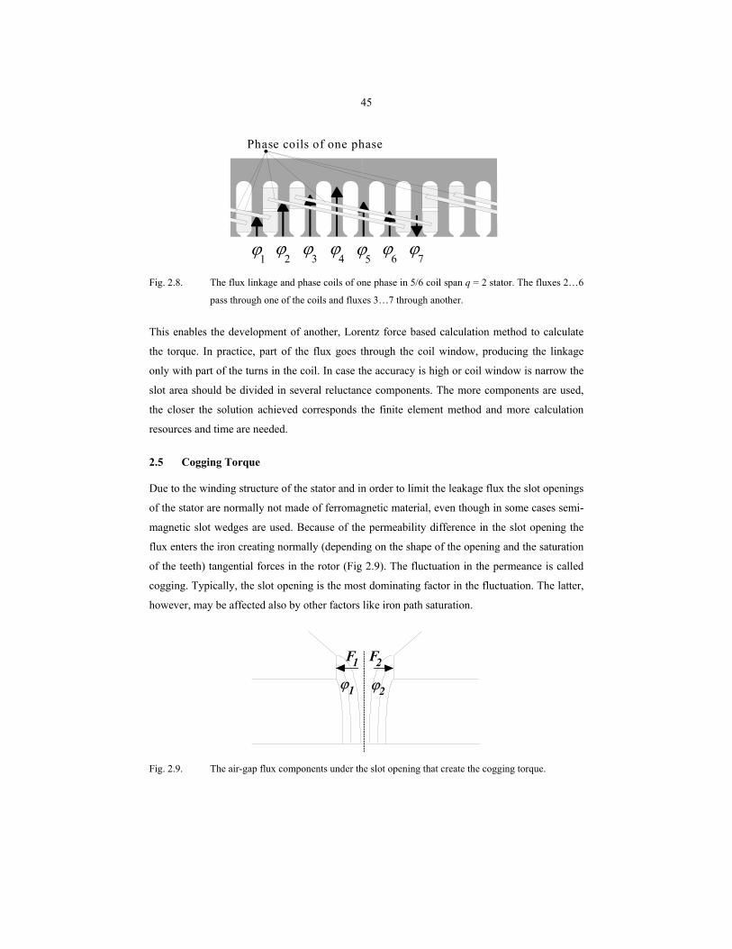
around them are used. Figure 2.8 shows part of the stator in a three-phase motor, the phase coils
of one phase and the flux in the teeth. For example, in one of the coils fluxes 2…6 create the
flux linkage.
45
ϕ1
ϕ2
ϕ3
ϕ4
ϕ5
ϕ6
ϕ7
Phase coils of one phase
Fig. 2.8. The flux linkage and phase coils of one phase in 5/6 coil span q = 2 stator. The fluxes 2…6
pass through one of the coils and fluxes 3…7 through another.
This enables the development of another, Lorentz force based calculation method to calculate
the torque. In practice, part of the flux goes through the coil window, producing the linkage
only with part of the turns in the coil. In case the accuracy is high or coil window is narrow the
slot area should be divided in several reluctance components. The more components are used,
the closer the solution achieved corresponds the finite element method and more calculation
resources and time are needed.
2.5 Cogging Torque
Due to the winding structure of the stator and in order to limit the leakage flux the slot openings
of the stator are normally not made of ferromagnetic material, even though in some cases semi-
magnetic slot wedges are used. Because of the permeability difference in the slot opening the
flux enters the iron creating normally (depending on the shape of the opening and the saturation
of the teeth) tangential forces in the rotor (Fig 2.9). The fluctuation in the permeance is called
cogging. Typically, the slot opening is the most dominating factor in the fluctuation. The latter,
however, may be affected also by other factors like iron path saturation.
ϕ1 ϕ2
F1 F2
Fig. 2.9. The air-gap flux components under the slot opening that create the cogging torque.
46
The flux in the slot opening area on different sides of the opening and in different slot openings
is typically not equal and thus these forces do not compensate each other. In the calculation it is
assumed that the flux entering the left side of the opening is the component left from the
geometrical centre of the slot according to figure 2.9. The calculated total instantaneous torque
of the motor is the sum of the flux linkage and permeance fluctuation components.
Proca et al. (1999) presented a similar approach to the radial flux motor based on the force
caused by the flux entering the slot opening sides. Their equation is rather complex compared to
the method presented above
( ) ( ) ,π22π
aM2PM
0
ssccog ∑
+
+= ssggRm
NB
NRLT θ
µθ (2.13)
where ga = 0 and ssg = 0 outside the slot opening, ga = w1 + δag and ssg = 1 on the left side of
the slot opening and ga = w2 + δag and ssg = 1 on the right side of the slot opening. w1 and w2
are distances from the calculation point to the slot opening edge. The result based on this
equation and Zhu’s (1993) BPM –model (eqn. 2.1) are close to FEM-calculations.
The general method to calculate the torque ripple is based on the rate of change with the angular
positionθ of the co-energy W’ in the air-gap (Li 1988)
θ
WTd
d ′= , (2.14)
where
∫=′ VB
W d2
d0
2
µθ . (2.15)
This method requires an accurate modelling of the air-gap and, in practice, a dividing of the air-
gap in to finite elements. When a precise model is used this method unquestionably gives more
accurate results than the analytical calculation. However, for example in the case of an axial
flux motor it should be decided for the 3D method.
47
2.6 Radial Flux and Axial Flux Motor Calculation
In a radial type motor all sections of the magnets have the same peripheral velocity with respect
to the stator windings and create force with the same radius. If the magnet has a constant
tangential width and thickness, the flux densities created by each section of the magnet can be
combined and the torque can be calculated using only one flux density curve. However, if the
magnets are skewed compared to the stator slots, the same air-gap flux density curve may be
used, but each section has a different phase angle compared to the stator field and calculation
must be carried out in several sections. If the slightest changes in the torque quality should be
studied the amount of slices appears to be a crucial factor since this defines the quality of the
calculation. The amount of circle ring sector slices needed should be found iteratively. The
amount of slices is set large enough when further increasing of the number of slices does not
improve anymore the result.
For the axial flux motor the torque calculation should be done in sections independent of the
magnet shape or skewing, because each radial section creates a force with different radius and
the torque is the sum of the sections. In axial and linear motors normally at least one side of the
permanent magnets is plane and magnetization throughout the magnet is parallel. In radial
motors magnetization may be also radial. This affects the air-gap flux density created by the
magnets. The type of magnetization can be used to affect the motor properties. Parallel
magnetization directs the flux towards the centre, making the flux density more sinusoidal,
whereas radial magnetization keeps the flux density more constant (trapezoidal) (Jahns 1996,
Sebastian 1996).
2.7 Calculation Procedure
Calculation starts with the definition of the motor geometry, the material properties and
calculation parameters. A selected number of radial slices defines the magnet. Each slice is
described with a pair of numbers. The first number indicates the relative width of the slice
compared to the width of the pole and the second indicates the distance from the centre of the
slice to the middle of the pole. This representation enables to define any shape of the magnet in
a simple but effective way. The only limitations that must be taken into consideration are that
the magnets should be of equal thickness (height) and that their relative length should not be
greater than unity. The stator and rotor iron materials are described with their specific BH-
curves. These curves are set up in separate files, and their number is not limited. The calculation
parameters required are given in table 2.1. The winding is defined with the turns Ns, the number
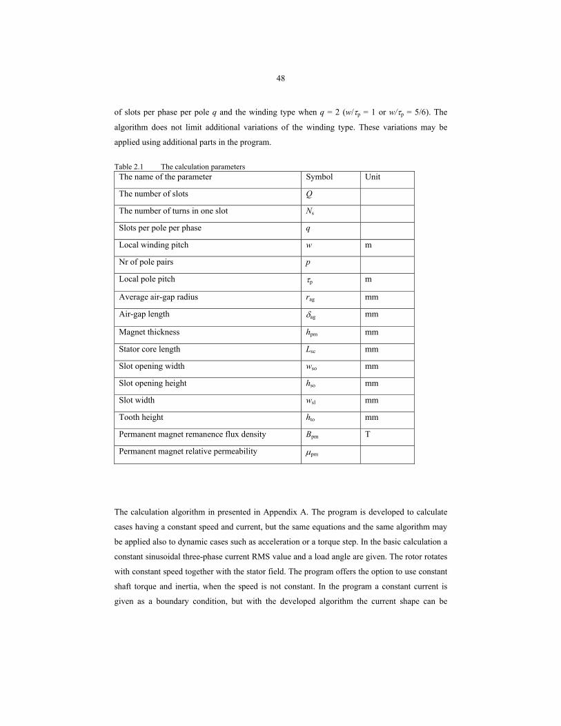
48
of slots per phase per pole q and the winding type when q = 2 (w/τp = 1 or w/τp = 5/6). The
algorithm does not limit additional variations of the winding type. These variations may be
applied using additional parts in the program.
Table 2.1 The calculation parameters The name of the parameter Symbol Unit
The number of slots Q
The number of turns in one slot Ns
Slots per pole per phase q
Local winding pitch w m
Nr of pole pairs p
Local pole pitch τp m
Average air-gap radius rag mm
Air-gap length δag mm
Magnet thickness hpm mm
Stator core length Lsc mm
Slot opening width wso mm
Slot opening height hso mm
Slot width wsl mm
Tooth height hto mm
Permanent magnet remanence flux density Bpm T
Permanent magnet relative permeability µpm
The calculation algorithm in presented in Appendix A. The program is developed to calculate
cases having a constant speed and current, but the same equations and the same algorithm may
be applied also to dynamic cases such as acceleration or a torque step. In the basic calculation a
constant sinusoidal three-phase current RMS value and a load angle are given. The rotor rotates
with constant speed together with the stator field. The program offers the option to use constant
shaft torque and inertia, when the speed is not constant. In the program a constant current is
given as a boundary condition, but with the developed algorithm the current shape can be
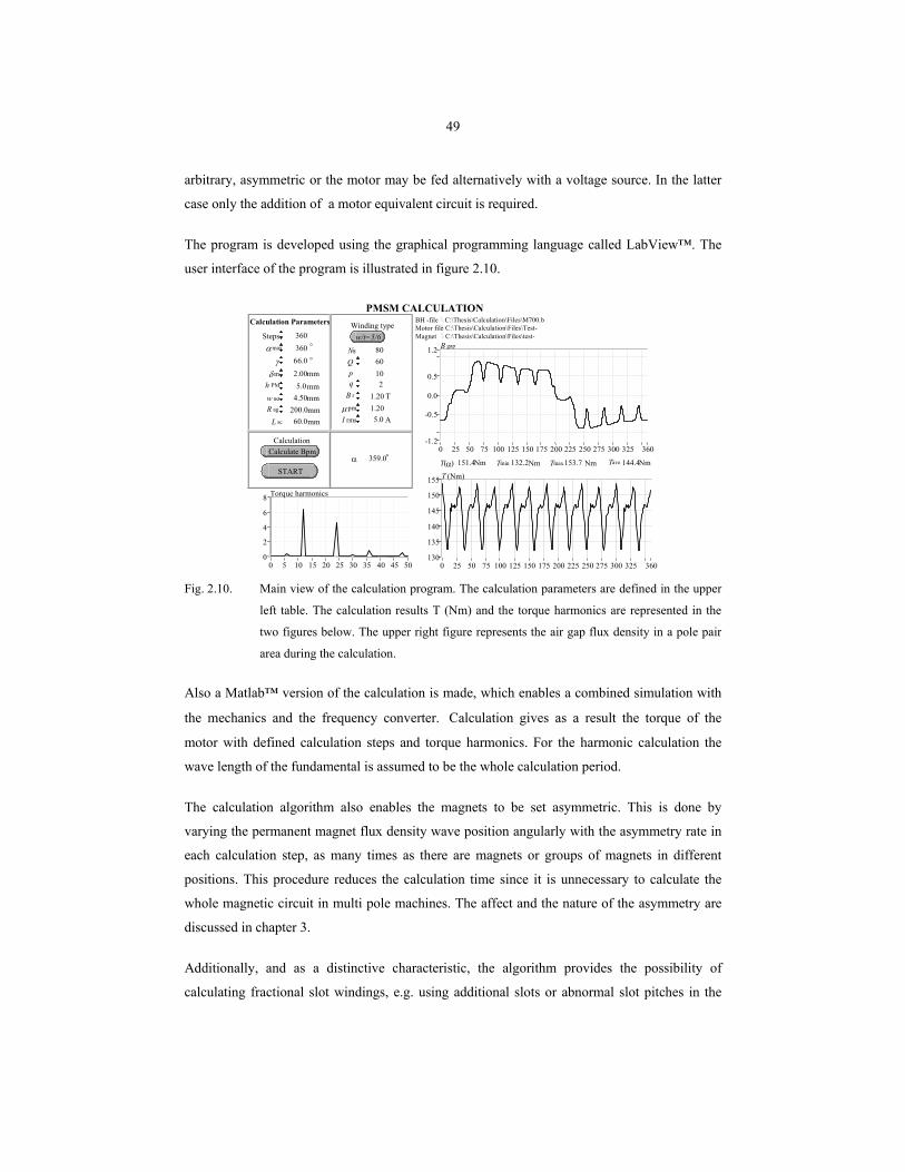
49
arbitrary, asymmetric or the motor may be fed alternatively with a voltage source. In the latter
case only the addition of a motor equivalent circuit is required.
The program is developed using the graphical programming language called LabView™. The
user interface of the program is illustrated in figure 2.10.
359.0α 151.4T(α)
1.2
-1.2
-0.5
0.0
0.5
360 0 25 50 75 100 125 150 175 200 225 250 275 300 325
B gap
1.20B r 1.20µ pm
10p
200.0 R ag 4.50 w so
60Q 66.0 γ
5.0I rms
Calculate Bpm Calculation
155
130
135
140
145
150
360 0 25 50 75 100 125 150 175 200 225 250 275 300 325
T (Nm)
360 Steps 360 α max
C:\Thesis\Calculation\Files\M700.bBH -fileC:\Thesis\Calculation\Files\Test-Motor file
60.0 L sc
80N s
8
0 2 4 6
500 5 10 15 20 25 30 35 40 45
Torque harmonics
144.4 Tave
2.00 δ m 5.0 h PM
mm
mm mm
A
Nm
mm
mm
T
°
°
Calculation Parameters
Nm
PMSM CALCULATION
°
START 132.2Tmin 153.7Tmax
2q
w/t=5/6Winding type
C:\Thesis\Calculation\Files\test-Magnet
Nm Nm
Fig. 2.10. Main view of the calculation program. The calculation parameters are defined in the upper
left table. The calculation results T (Nm) and the torque harmonics are represented in the
two figures below. The upper right figure represents the air gap flux density in a pole pair
area during the calculation.
Also a Matlab™ version of the calculation is made, which enables a combined simulation with
the mechanics and the frequency converter. Calculation gives as a result the torque of the
motor with defined calculation steps and torque harmonics. For the harmonic calculation the
wave length of the fundamental is assumed to be the whole calculation period.
The calculation algorithm also enables the magnets to be set asymmetric. This is done by
varying the permanent magnet flux density wave position angularly with the asymmetry rate in
each calculation step, as many times as there are magnets or groups of magnets in different
positions. This procedure reduces the calculation time since it is unnecessary to calculate the
whole magnetic circuit in multi pole machines. The affect and the nature of the asymmetry are
discussed in chapter 3.
Additionally, and as a distinctive characteristic, the algorithm provides the possibility of
calculating fractional slot windings, e.g. using additional slots or abnormal slot pitches in the
50
stator. This is also explained in chapter 3. Here, the stator field is asymmetric between the
poles, which means that, instead of one pole pair, the whole motor must be modelled and
calculated.
2.8 Conclusions
An analytical model for the axial flux permanent magnet motor was developed. The model
divides the calculation of an axial flux machine in several radial circles and may thus be used to
accurately calculate the torque ripple behaviour of axial-flux permanent magnet synchronous
machines. Comparison of the results with the results given by FEM proves that analytical
methods may be applied to calculate the air-gap flux density created by the permanent magnets.
In the numerical calculation the Lorentz Force based flux linkage method is proven to be the
most suitable method since it gives fast reliable results. The calculation allows easy parameter
definition and also consideration of certain non-linearities and asymmetries.
51
3 Torque Vibration
The torque vibration of an electric machine is the sum of different excitations created by
multiple sources. Besides the machine itself also the power source may generate a torque ripple.
The current shape, especially in frequency converter drives, often differs to some degree from
the sinusoidal, which inevitably creates a torque ripple in machines developed for sinusoidal
supply. Another source of excitation may be the mechanics . These, however, also amplify (and
dampen) the frequencies differently. This chapter studies the influence of different machine
components on the torque quality. The forming and the placement of the permanent magnets,
the magnetic circuit dimensions, the winding arrangements and different types of asymmetry
are discussed.
Vibration excitations are caused by the power supply, the structure of the electrical circuit
(winding arrangements and physical asymmetry of the assembly), the mechanical structure of
the magnetic circuit, possible eccentricity and etc. In principle, in an electric machine electro-
magnetic torque pulsations are generated by two different effects: 1) Stator and rotor mmf
harmonic interactions and 2) reluctance discontinuities in the whole magnetic circuit.
The stator harmonic mmfs reach a practical minimum when the number of slots per phase and
pole q is as large as feasible and when w/τp= 5/6 short pitch windings are used (Vogt 1983).
However, in a multi-pole machine there is often no space to increase the value of q and thus the
designer has to apply slot numbers per pole and phase near to 1 and 2. In some recent articles
fractional slot windings with q = 0.25, q = 0.4 and q = 0.5 are reported (Koch 2002). When
above-mentioned values for the fractional slot winding are applied the torque producing
tangential electro-magnetic stress reaches very high values, as high as e.g. 58 kN/m2.
In a PMSM the thickness variation of the magnets along the pole pitch or the contour shape of
uniform thickness permanent magnets may be selected purely sinusoidal which, in principle,
eliminates all torque vibrations generated by the stator and rotor mmfs (Pyrhönen, 1999). Using
a smooth rotor steel core surface guarantees that no harmonic reluctance torques can possibly be
generated in interaction between the stator harmonics and rotor reluctance variations.
Although the sinusoidal form of the permanent magnets produces also a low cogging, there is,
however, no guarantee that it will give the minimum cogging torque. Different measures are
needed for the cogging torque than for the stator generated harmonic torques. The intersection
52
point of the permanent magnet edge curve and the stator slot opening should move at a constant
speed and when a magnet has totally passed the slot opening the edge of another magnet should
take over in order that the process could continue smoothly.
Even though the amplitude of each component would stay constant, the result in the torque
vibration depends on the frequency response of the mechanical structure. Typically, the
structure may include one or more of the following components: the motor (especially rotor),
shaft, clutches, gearbox and the regulating unit. The more complex is the structure, the bigger
number of rated eigen-frequencies can be found, and the more likely vibration problems may
occur. It has to be noticed, that in the case of a gearbox, also the frequency of the excitations is
changed according to the gear ratio.
3.1 Calculation Parameters
There are several different factors that influence the torque vibration of an electric motor. To
optimise the motor structure, many of these factors should be analysed in calculations based on
the analytical equations introduced in chapter two. The example calculations in this chapter are
performed with an axial flux motor having the basic parameters given in table 3.1. These
parameters are kept constant and the changes made concern the winding, permanent magnet
material properties and geometrical details. Also the effects of different asymmetry parameters
are considered. Some of these factors are dealt with in the test motor measurements and in
corresponding calculations and they are discussed in chapter four,. Unless otherwise stated the
calculations are carried out with a permanent magnet form, which has radial edges that are
parallel to the slots (fig. 3.1). This shape is most responsive to cogging and thus the effects of
the changes are easier to determine.
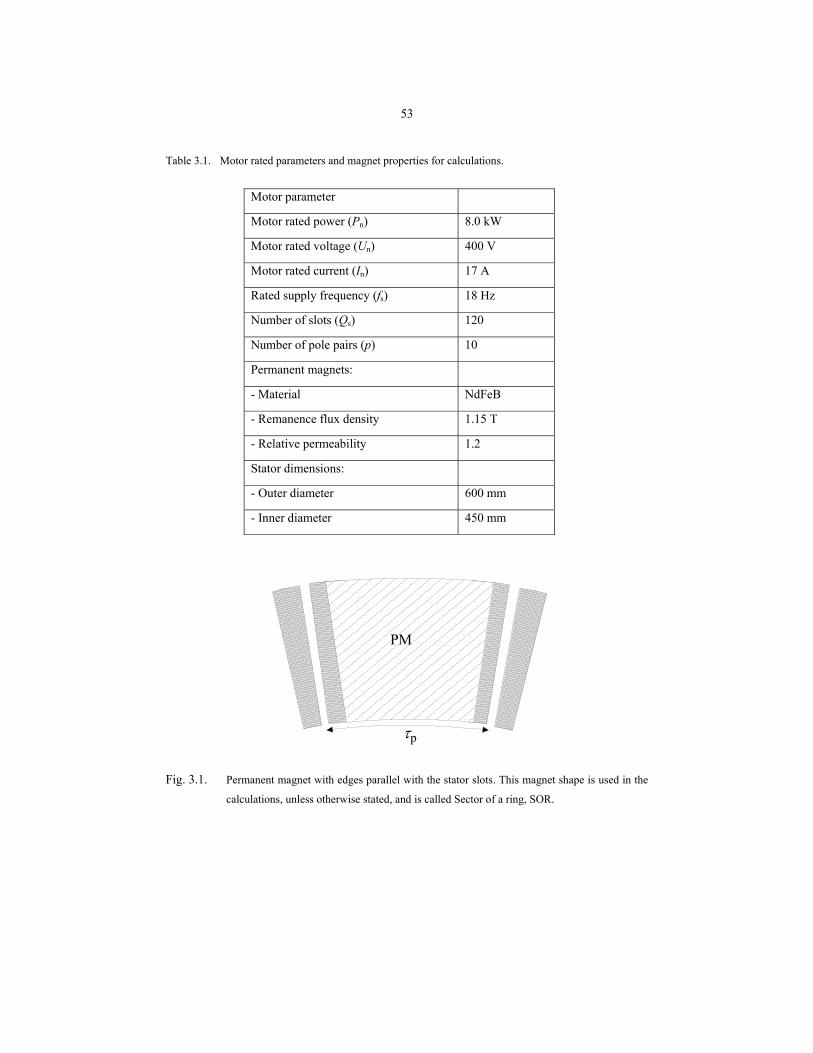
53
Table 3.1. Motor rated parameters and magnet properties for calculations.
Motor parameter
Motor rated power (Pn) 8.0 kW
Motor rated voltage (Un) 400 V
Motor rated current (In) 17 A
Rated supply frequency (fs) 18 Hz
Number of slots (Qs) 120
Number of pole pairs (p) 10
Permanent magnets:
- Material NdFeB
- Remanence flux density 1.15 T
- Relative permeability 1.2
Stator dimensions:
- Outer diameter 600 mm
- Inner diameter 450 mm
PM
τp
Fig. 3.1. Permanent magnet with edges parallel with the stator slots. This magnet shape is used in the
calculations, unless otherwise stated, and is called Sector of a ring, SOR.
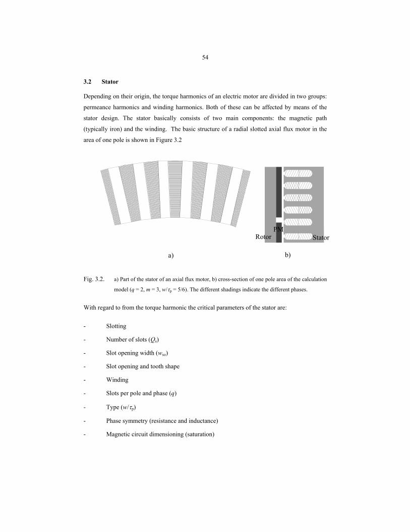
54
3.2 Stator
Depending on their origin, the torque harmonics of an electric motor are divided in two groups:
permeance harmonics and winding harmonics. Both of these can be affected by means of the
stator design. The stator basically consists of two main components: the magnetic path
(typically iron) and the winding. The basic structure of a radial slotted axial flux motor in the
area of one pole is shown in Figure 3.2
StatorRotorPM
b)a)
Fig. 3.2. a) Part of the stator of an axial flux motor, b) cross-section of one pole area of the calculation
model (q = 2, m = 3, w/τp = 5/6). The different shadings indicate the different phases.
With regard to from the torque harmonic the critical parameters of the stator are:
- Slotting
- Number of slots (Qs)
- Slot opening width (wso)
- Slot opening and tooth shape
- Winding
- Slots per pole and phase (q)
- Type (w/τp)
- Phase symmetry (resistance and inductance)
- Magnetic circuit dimensioning (saturation)
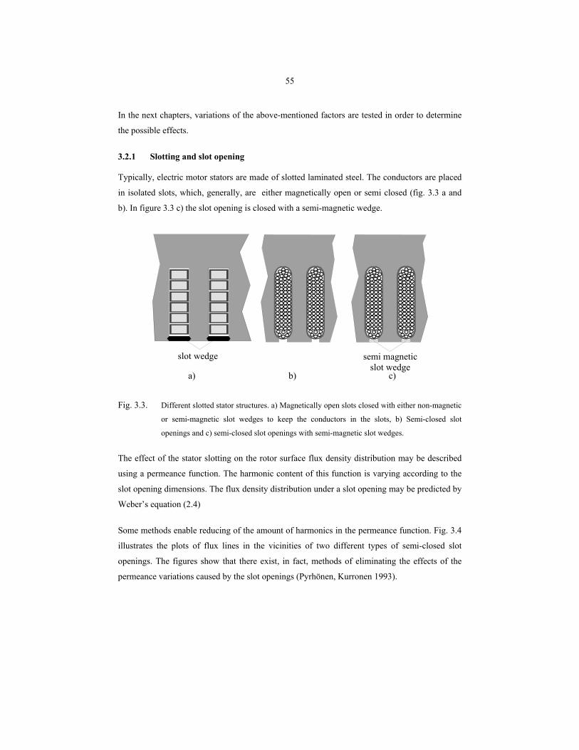
55
In the next chapters, variations of the above-mentioned factors are tested in order to determine
the possible effects.
3.2.1 Slotting and slot opening
Typically, electric motor stators are made of slotted laminated steel. The conductors are placed
in isolated slots, which, generally, are either magnetically open or semi closed (fig. 3.3 a and
b). In figure 3.3 c) the slot opening is closed with a semi-magnetic wedge.
a) b) c)
slot wedge semi magneticslot wedge
Fig. 3.3. Different slotted stator structures. a) Magnetically open slots closed with either non-magnetic
or semi-magnetic slot wedges to keep the conductors in the slots, b) Semi-closed slot
openings and c) semi-closed slot openings with semi-magnetic slot wedges.
The effect of the stator slotting on the rotor surface flux density distribution may be described
using a permeance function. The harmonic content of this function is varying according to the
slot opening dimensions. The flux density distribution under a slot opening may be predicted by
Weber’s equation (2.4)
Some methods enable reducing of the amount of harmonics in the permeance function. Fig. 3.4
illustrates the plots of flux lines in the vicinities of two different types of semi-closed slot
openings. The figures show that there exist, in fact, methods of eliminating the effects of the
permeance variations caused by the slot openings (Pyrhönen, Kurronen 1993).
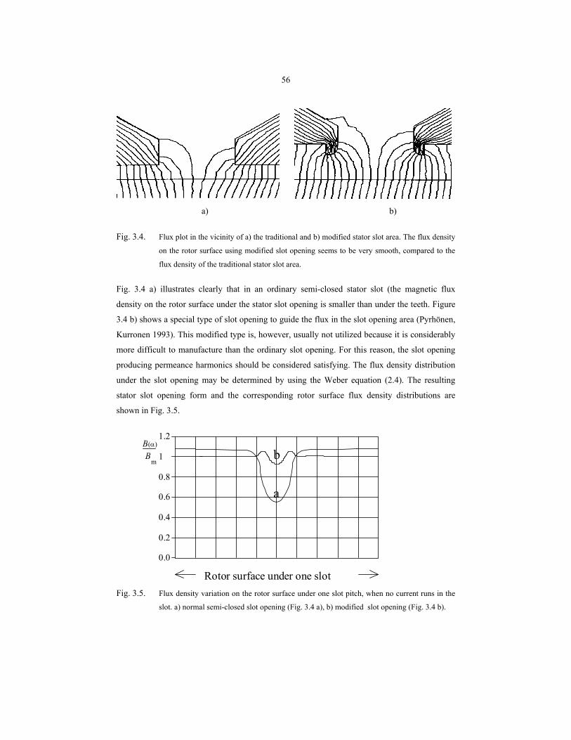
56
a) b)
Fig. 3.4. Flux plot in the vicinity of a) the traditional and b) modified stator slot area. The flux density
on the rotor surface using modified slot opening seems to be very smooth, compared to the
flux density of the traditional stator slot area.
Fig. 3.4 a) illustrates clearly that in an ordinary semi-closed stator slot (the magnetic flux
density on the rotor surface under the stator slot opening is smaller than under the teeth. Figure
3.4 b) shows a special type of slot opening to guide the flux in the slot opening area (Pyrhönen,
Kurronen 1993). This modified type is, however, usually not utilized because it is considerably
more difficult to manufacture than the ordinary slot opening. For this reason, the slot opening
producing permeance harmonics should be considered satisfying. The flux density distribution
under the slot opening may be determined by using the Weber equation (2.4). The resulting
stator slot opening form and the corresponding rotor surface flux density distributions are
shown in Fig. 3.5.
B B
m 1 0.8 0.6 0.4 0.2 0.0
1.2
Rotor surface under one slot
a
b(α)
Fig. 3.5. Flux density variation on the rotor surface under one slot pitch, when no current runs in the
slot. a) normal semi-closed slot opening (Fig. 3.4 a), b) modified slot opening (Fig. 3.4 b).
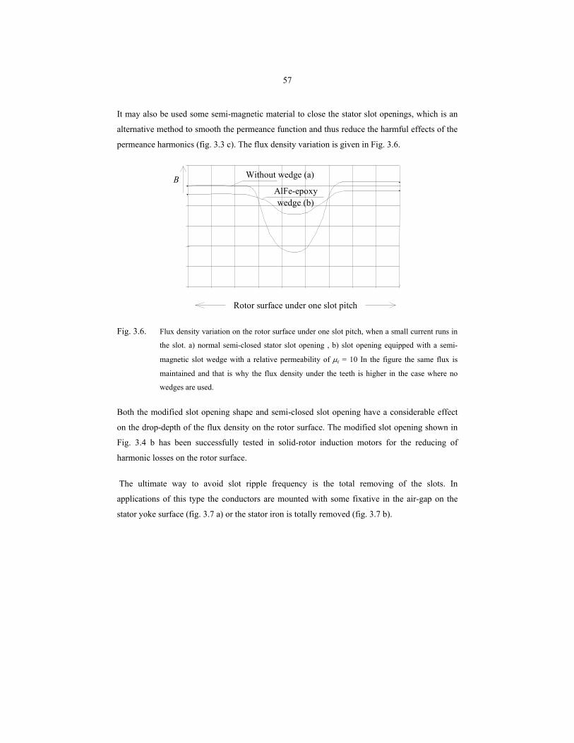
57
It may also be used some semi-magnetic material to close the stator slot openings, which is an
alternative method to smooth the permeance function and thus reduce the harmful effects of the
permeance harmonics (fig. 3.3 c). The flux density variation is given in Fig. 3.6.
Rotor surface under one slot pitch
B Without wedge (a)
AlFe-epoxy
wedge (b)
Fig. 3.6. Flux density variation on the rotor surface under one slot pitch, when a small current runs in
the slot. a) normal semi-closed stator slot opening , b) slot opening equipped with a semi-
magnetic slot wedge with a relative permeability of µr = 10 In the figure the same flux is
maintained and that is why the flux density under the teeth is higher in the case where no
wedges are used.
Both the modified slot opening shape and semi-closed slot opening have a considerable effect
on the drop-depth of the flux density on the rotor surface. The modified slot opening shown in
Fig. 3.4 b has been successfully tested in solid-rotor induction motors for the reducing of
harmonic losses on the rotor surface.
The ultimate way to avoid slot ripple frequency is the total removing of the slots. In
applications of this type the conductors are mounted with some fixative in the air-gap on the
stator yoke surface (fig. 3.7 a) or the stator iron is totally removed (fig. 3.7 b).
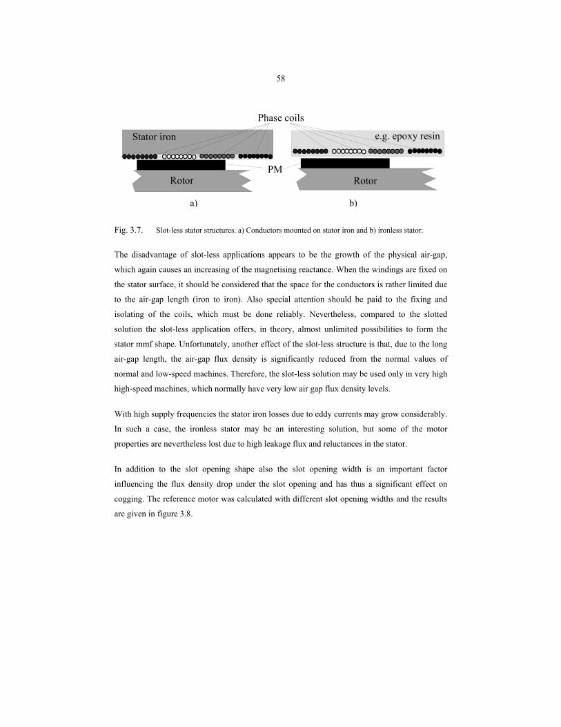
58
Stator iron
Phase coils
e.g. epoxy resin
Rotor RotorPM
a) b)
Fig. 3.7. Slot-less stator structures. a) Conductors mounted on stator iron and b) ironless stator.
The disadvantage of slot-less applications appears to be the growth of the physical air-gap,
which again causes an increasing of the magnetising reactance. When the windings are fixed on
the stator surface, it should be considered that the space for the conductors is rather limited due
to the air-gap length (iron to iron). Also special attention should be paid to the fixing and
isolating of the coils, which must be done reliably. Nevertheless, compared to the slotted
solution the slot-less application offers, in theory, almost unlimited possibilities to form the
stator mmf shape. Unfortunately, another effect of the slot-less structure is that, due to the long
air-gap length, the air-gap flux density is significantly reduced from the normal values of
normal and low-speed machines. Therefore, the slot-less solution may be used only in very high
high-speed machines, which normally have very low air gap flux density levels.
With high supply frequencies the stator iron losses due to eddy currents may grow considerably.
In such a case, the ironless stator may be an interesting solution, but some of the motor
properties are nevertheless lost due to high leakage flux and reluctances in the stator.
In addition to the slot opening shape also the slot opening width is an important factor
influencing the flux density drop under the slot opening and has thus a significant effect on
cogging. The reference motor was calculated with different slot opening widths and the results
are given in figure 3.8.
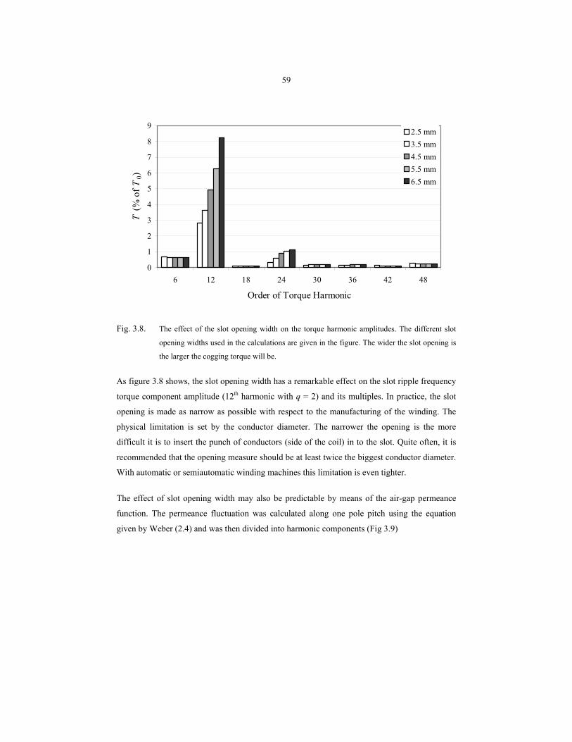
59
0
1
2
3
4
5
6
7
8
9
6 12 18 24 30 36 42 48
Order of Torque Harmonic
T (%
of T
0)2.5 mm3.5 mm4.5 mm5.5 mm6.5 mm
Fig. 3.8. The effect of the slot opening width on the torque harmonic amplitudes. The different slot
opening widths used in the calculations are given in the figure. The wider the slot opening is
the larger the cogging torque will be.
As figure 3.8 shows, the slot opening width has a remarkable effect on the slot ripple frequency
torque component amplitude (12th harmonic with q = 2) and its multiples. In practice, the slot
opening is made as narrow as possible with respect to the manufacturing of the winding. The
physical limitation is set by the conductor diameter. The narrower the opening is the more
difficult it is to insert the punch of conductors (side of the coil) in to the slot. Quite often, it is
recommended that the opening measure should be at least twice the biggest conductor diameter.
With automatic or semiautomatic winding machines this limitation is even tighter.
The effect of slot opening width may also be predictable by means of the air-gap permeance
function. The permeance fluctuation was calculated along one pole pitch using the equation
given by Weber (2.4) and was then divided into harmonic components (Fig 3.9)
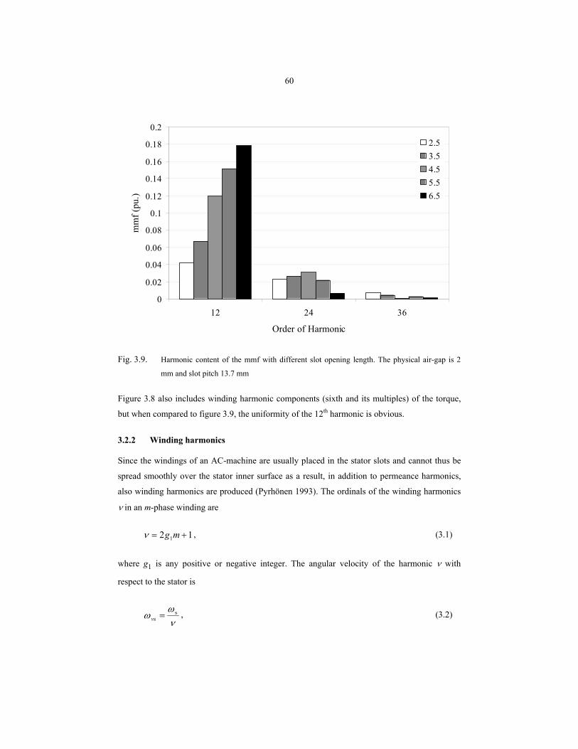
60
0
0.02
0.04
0.06
0.08
0.1
0.12
0.14
0.16
0.18
0.2
12 24 36
Order of Harmonic
mm
f (pu
.)2.53.54.55.56.5
Fig. 3.9. Harmonic content of the mmf with different slot opening length. The physical air-gap is 2
mm and slot pitch 13.7 mm
Figure 3.8 also includes winding harmonic components (sixth and its multiples) of the torque,
but when compared to figure 3.9, the uniformity of the 12th harmonic is obvious.
3.2.2 Winding harmonics
Since the windings of an AC-machine are usually placed in the stator slots and cannot thus be
spread smoothly over the stator inner surface as a result, in addition to permeance harmonics,
also winding harmonics are produced (Pyrhönen 1993). The ordinals of the winding harmonics
ν in an m-phase winding are
12 1 += mgν , (3.1)
where g1 is any positive or negative integer. The angular velocity of the harmonic ν with
respect to the stator is
νω
ω ss =ν , (3.2)
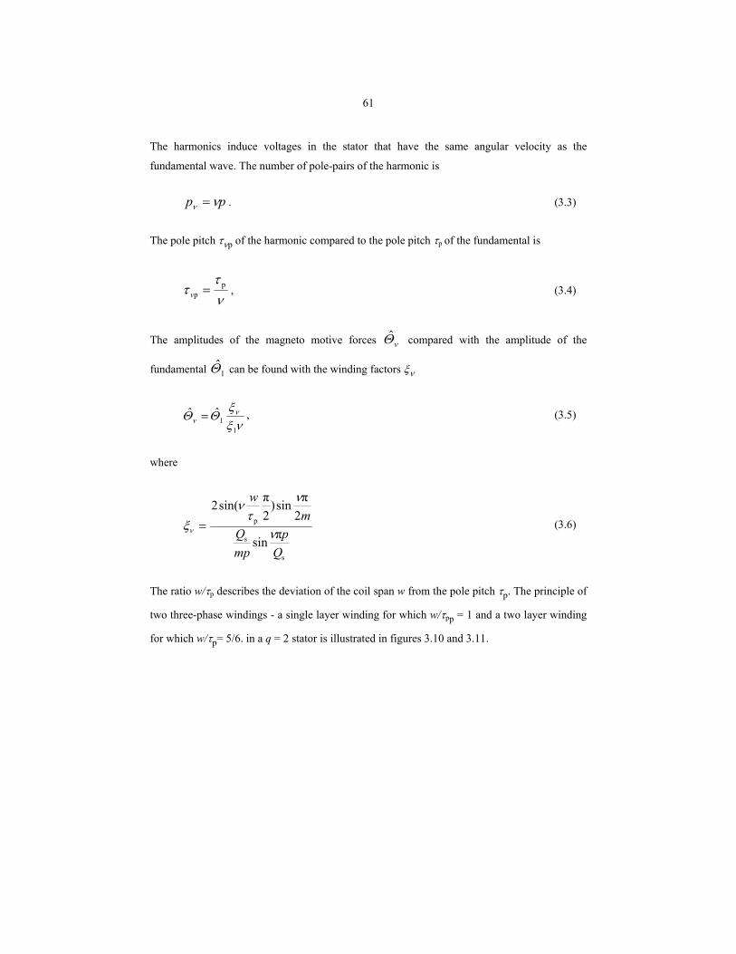
61
The harmonics induce voltages in the stator that have the same angular velocity as the
fundamental wave. The number of pole-pairs of the harmonic is
pp νν = . (3.3)
The pole pitch τνp of the harmonic compared to the pole pitch τp of the fundamental is
ντ
τ pp =ν , (3.4)
The amplitudes of the magneto motive forces νΘ compared with the amplitude of the
fundamental 1Θ can be found with the winding factors ξν
νξ
ξΘΘ ν
ν1
1ˆˆ = , (3.5)
where
s
s
p
πsin
2πsin)
2πsin(2
Qp
mpQ
mw
ν
ντ
νξν = (3.6)
The ratio w/τp describes the deviation of the coil span w from the pole pitch τp. The principle of
two three-phase windings - a single layer winding for which w/τpp = 1 and a two layer winding
for which w/τp= 5/6. in a q = 2 stator is illustrated in figures 3.10 and 3.11.
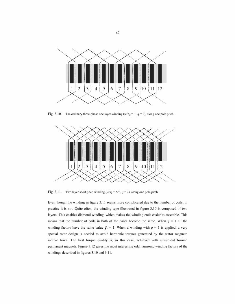
62
1 32 4 5 6 7 8 9 10 11 12
Fig. 3.10. The ordinary three-phase one layer winding (w/τ p = 1, q = 2), along one pole pitch.
1 32 4 5 6 7 8 9 10 11 12
Fig. 3.11. Two layer short pitch winding (w/τp = 5/6, q = 2), along one pole pitch.
Even though the winding in figure 3.11 seems more complicated due to the number of coils, in
practice it is not. Quite often, the winding type illustrated in figure 3.10 is composed of two
layers. This enables diamond winding, which makes the winding ends easier to assemble. This
means that the number of coils in both of the cases become the same. When q = 1 all the
winding factors have the same value ξν = 1. When a winding with q = 1 is applied, a very
special rotor design is needed to avoid harmonic torques generated by the stator magneto
motive force. The best torque quality is, in this case, achieved with sinusoidal formed
permanent magnets. Figure 3.12 gives the most interesting odd harmonic winding factors of the
windings described in figures 3.10 and 3.11.
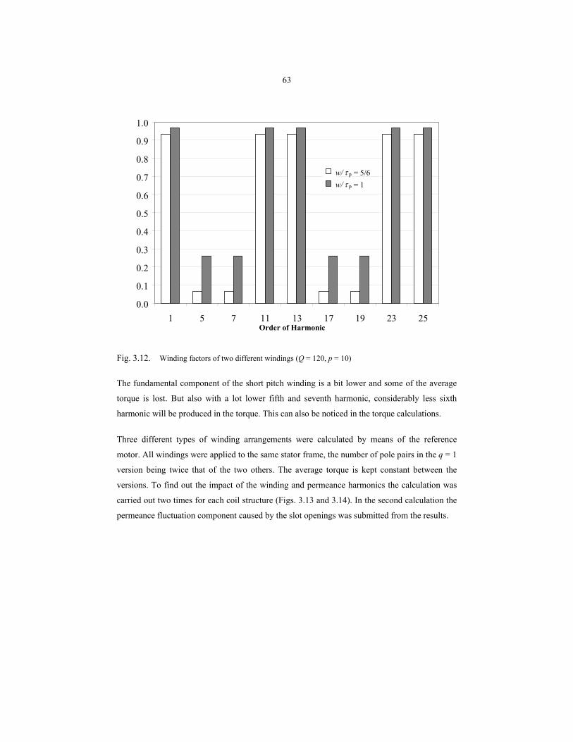
63
Fig. 3.12. Winding factors of two different windings (Q = 120, p = 10)
The fundamental component of the short pitch winding is a bit lower and some of the average
torque is lost. But also with a lot lower fifth and seventh harmonic, considerably less sixth
harmonic will be produced in the torque. This can also be noticed in the torque calculations.
Three different types of winding arrangements were calculated by means of the reference
motor. All windings were applied to the same stator frame, the number of pole pairs in the q = 1
version being twice that of the two others. The average torque is kept constant between the
versions. To find out the impact of the winding and permeance harmonics the calculation was
carried out two times for each coil structure (Figs. 3.13 and 3.14). In the second calculation the
permeance fluctuation component caused by the slot openings was submitted from the results.
0.0
0.1
0.2
0.3
0.4
0.5
0.6
0.7
0.8
0.9
1.0
1 5 7 11 13 17 19 23 25
w/ τ p = 5/6w/ τ p = 1
Order of Harmonic
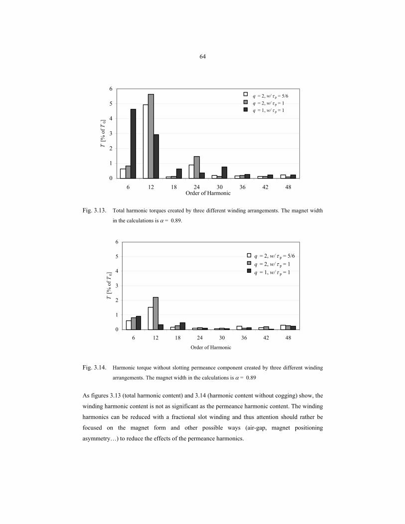
64
0
1
2
3
4
5
6
6 12 18 24 30 36 42 48Order of Harmonic
T [%
of T
0]q = 2, w/ τ p = 5/6q = 2, w/ τ p = 1q = 1, w/ τ p = 1
Fig. 3.13. Total harmonic torques created by three different winding arrangements. The magnet width
in the calculations is α = 0.89.
0
1
2
3
4
5
6
6 12 18 24 30 36 42 48
Order of Harmonic
T [%
of T
0]
q = 2, w/ τ p = 5/6q = 2, w/ τ p = 1q = 1, w/ τ p = 1
Fig. 3.14. Harmonic torque without slotting permeance component created by three different winding
arrangements. The magnet width in the calculations is α = 0.89
As figures 3.13 (total harmonic content) and 3.14 (harmonic content without cogging) show, the
winding harmonic content is not as significant as the permeance harmonic content. The winding
harmonics can be reduced with a fractional slot winding and thus attention should rather be
focused on the magnet form and other possible ways (air-gap, magnet positioning
asymmetry…) to reduce the effects of the permeance harmonics.
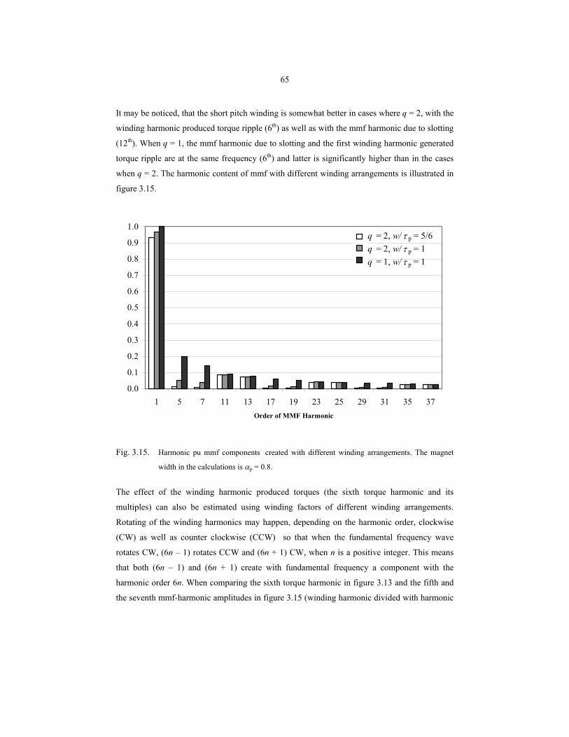
65
It may be noticed, that the short pitch winding is somewhat better in cases where q = 2, with the
winding harmonic produced torque ripple (6th) as well as with the mmf harmonic due to slotting
(12th). When q = 1, the mmf harmonic due to slotting and the first winding harmonic generated
torque ripple are at the same frequency (6th) and latter is significantly higher than in the cases
when q = 2. The harmonic content of mmf with different winding arrangements is illustrated in
figure 3.15.
0.0
0.1
0.2
0.3
0.4
0.5
0.6
0.7
0.8
0.9
1.0
1 5 7 11 13 17 19 23 25 29 31 35 37Order of MMF Harmonic
q = 2, w/ τ p = 5/6q = 2, w/ τ p = 1q = 1, w/ τ p = 1
Fig. 3.15. Harmonic pu mmf components created with different winding arrangements. The magnet
width in the calculations is αp = 0.8.
The effect of the winding harmonic produced torques (the sixth torque harmonic and its
multiples) can also be estimated using winding factors of different winding arrangements.
Rotating of the winding harmonics may happen, depending on the harmonic order, clockwise
(CW) as well as counter clockwise (CCW) so that when the fundamental frequency wave
rotates CW, (6n – 1) rotates CCW and (6n + 1) CW, when n is a positive integer. This means
that both (6n – 1) and (6n + 1) create with fundamental frequency a component with the
harmonic order 6n. When comparing the sixth torque harmonic in figure 3.13 and the fifth and
the seventh mmf-harmonic amplitudes in figure 3.15 (winding harmonic divided with harmonic
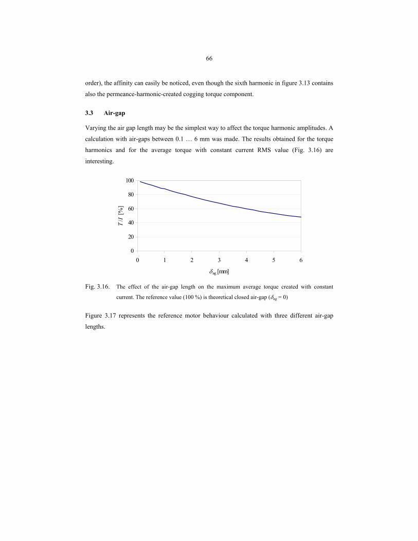
66
order), the affinity can easily be noticed, even though the sixth harmonic in figure 3.13 contains
also the permeance-harmonic-created cogging torque component.
3.3 Air-gap
Varying the air gap length may be the simplest way to affect the torque harmonic amplitudes. A
calculation with air-gaps between 0.1 … 6 mm was made. The results obtained for the torque
harmonics and for the average torque with constant current RMS value (Fig. 3.16) are
interesting.
0
20
40
60
80
100
0 1 2 3 4 5 6
δag [mm]
T/I
[%]
Fig. 3.16. The effect of the air-gap length on the maximum average torque created with constant
current. The reference value (100 %) is theoretical closed air-gap (δag = 0)
Figure 3.17 represents the reference motor behaviour calculated with three different air-gap
lengths.
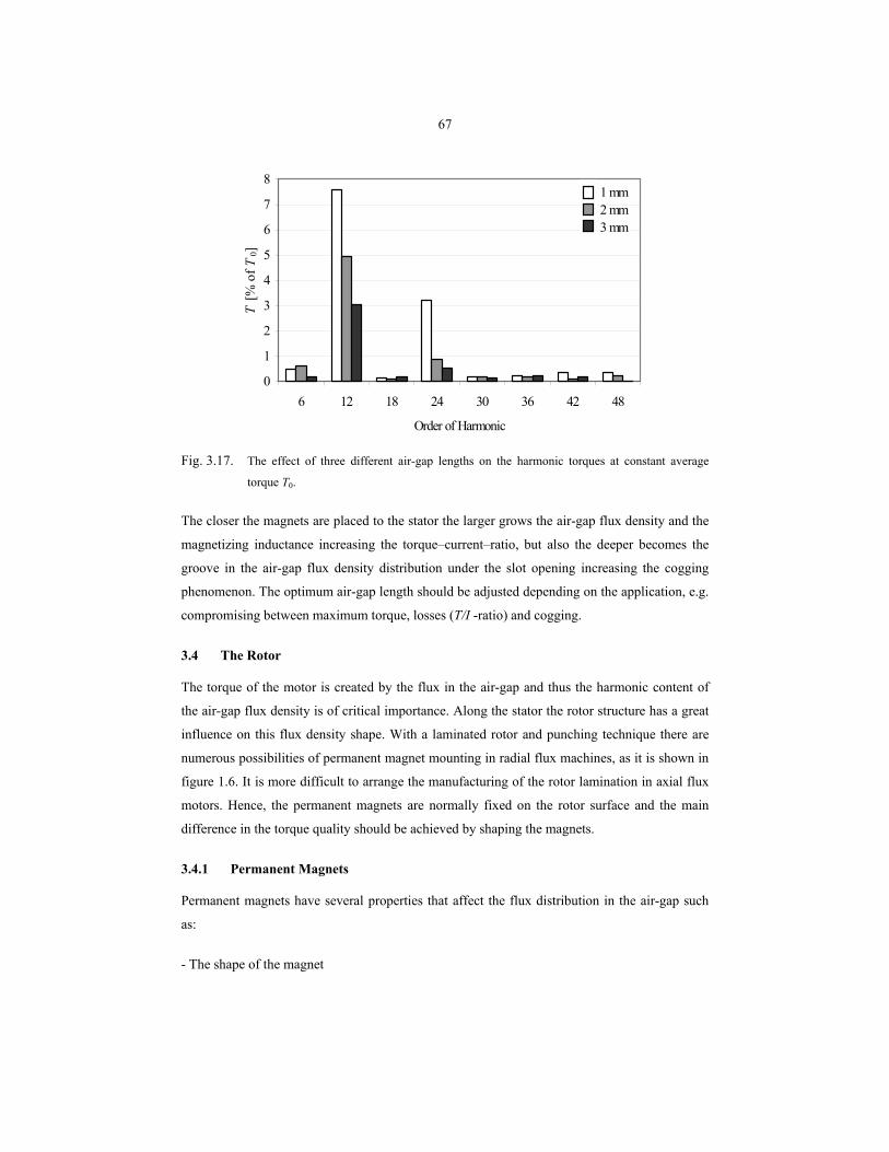
67
0
1
2
3
4
5
6
7
8
6 12 18 24 30 36 42 48
Order of Harmonic
T [%
of T
0]
1 mm2 mm3 mm
Fig. 3.17. The effect of three different air-gap lengths on the harmonic torques at constant average
torque T0.
The closer the magnets are placed to the stator the larger grows the air-gap flux density and the
magnetizing inductance increasing the torque–current–ratio, but also the deeper becomes the
groove in the air-gap flux density distribution under the slot opening increasing the cogging
phenomenon. The optimum air-gap length should be adjusted depending on the application, e.g.
compromising between maximum torque, losses (T/I -ratio) and cogging.
3.4 The Rotor
The torque of the motor is created by the flux in the air-gap and thus the harmonic content of
the air-gap flux density is of critical importance. Along the stator the rotor structure has a great
influence on this flux density shape. With a laminated rotor and punching technique there are
numerous possibilities of permanent magnet mounting in radial flux machines, as it is shown in
figure 1.6. It is more difficult to arrange the manufacturing of the rotor lamination in axial flux
motors. Hence, the permanent magnets are normally fixed on the rotor surface and the main
difference in the torque quality should be achieved by shaping the magnets.
3.4.1 Permanent Magnets
Permanent magnets have several properties that affect the flux distribution in the air-gap such
as:
- The shape of the magnet
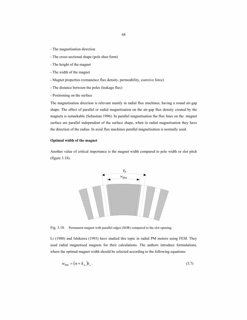
68
- The magnetisation direction
- The cross-sectional shape (pole shoe form)
- The height of the magnet
- The width of the magnet
- Magnet properties (remanence flux density, permeability, coercive force)
- The distance between the poles (leakage flux)
- Positioning on the surface
The magnetisation direction is relevant mainly in radial flux machines, having a round air-gap
shape. The effect of parallel or radial magnetisation on the air-gap flux density created by the
magnets is remarkable (Sebastian 1996). In parallel magnetisation the flux lines on the magnet
surface are parallel independent of the surface shape, when in radial magnetisation they have
the direction of the radius. In axial flux machines parallel magnetisation is normally used.
Optimal width of the magnet
Another value of critical importance is the magnet width compared to pole width or slot pitch
(figure 3.18).
pτwPM
Fig. 3.18. Permanent magnet with parallel edges (SOR) compared to the slot opening.
Li (1988) and Ishikawa (1993) have studied this topic in radial PM motors using FEM. They
used radial magnetised magnets for their calculations. The authors introduce formulations,
where the optimal magnet width should be selected according to the following equations:
( ) swPM τknw += . (3.7)
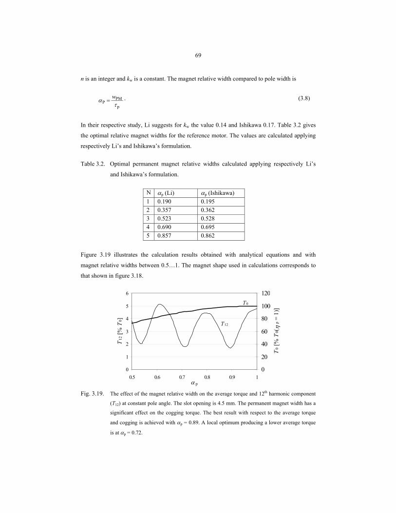
69
n is an integer and kw is a constant. The magnet relative width compared to pole width is
p
PMP τ
α w= . (3.8)
In their respective study, Li suggests for kw the value 0.14 and Ishikawa 0.17. Table 3.2 gives
the optimal relative magnet widths for the reference motor. The values are calculated applying
respectively Li’s and Ishikawa’s formulation.
Table 3.2. Optimal permanent magnet relative widths calculated applying respectively Li’s
and Ishikawa’s formulation.
N αp (Li) αp (Ishikawa) 1 0.190 0.195 2 0.357 0.362 3 0.523 0.528 4 0.690 0.695 5 0.857 0.862
Figure 3.19 illustrates the calculation results obtained with analytical equations and with
magnet relative widths between 0.5…1. The magnet shape used in calculations corresponds to
that shown in figure 3.18.
0
1
2
3
4
5
6
0.5 0.6 0.7 0.8 0.9 1α p
T12
[% T
0]
0
20
40
60
80
100
120
T0 [
% T
0(η
p = 1
)] T0
T12
Fig. 3.19. The effect of the magnet relative width on the average torque and 12th harmonic component
(T12) at constant pole angle. The slot opening is 4.5 mm. The permanent magnet width has a
significant effect on the cogging torque. The best result with respect to the average torque
and cogging is achieved with αp = 0.89. A local optimum producing a lower average torque
is at αp = 0.72.
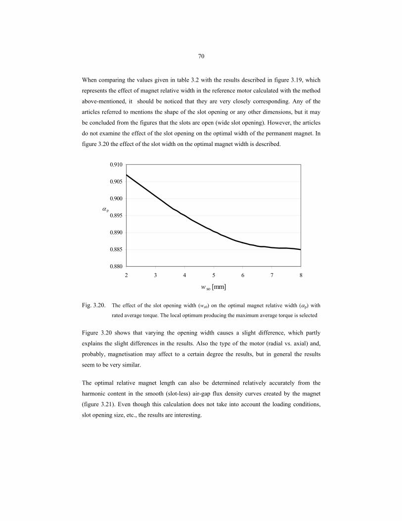
70
When comparing the values given in table 3.2 with the results described in figure 3.19, which
represents the effect of magnet relative width in the reference motor calculated with the method
above-mentioned, it should be noticed that they are very closely corresponding. Any of the
articles referred to mentions the shape of the slot opening or any other dimensions, but it may
be concluded from the figures that the slots are open (wide slot opening). However, the articles
do not examine the effect of the slot opening on the optimal width of the permanent magnet. In
figure 3.20 the effect of the slot width on the optimal magnet width is described.
0.880
0.885
0.890
0.895
0.900
0.905
0.910
2 3 4 5 6 7 8
w so [mm]
α p
Fig. 3.20. The effect of the slot opening width (ws0) on the optimal magnet relative width (αp) with
rated average torque. The local optimum producing the maximum average torque is selected
Figure 3.20 shows that varying the opening width causes a slight difference, which partly
explains the slight differences in the results. Also the type of the motor (radial vs. axial) and,
probably, magnetisation may affect to a certain degree the results, but in general the results
seem to be very similar.
The optimal relative magnet length can also be determined relatively accurately from the
harmonic content in the smooth (slot-less) air-gap flux density curves created by the magnet
(figure 3.21). Even though this calculation does not take into account the loading conditions,
slot opening size, etc., the results are interesting.
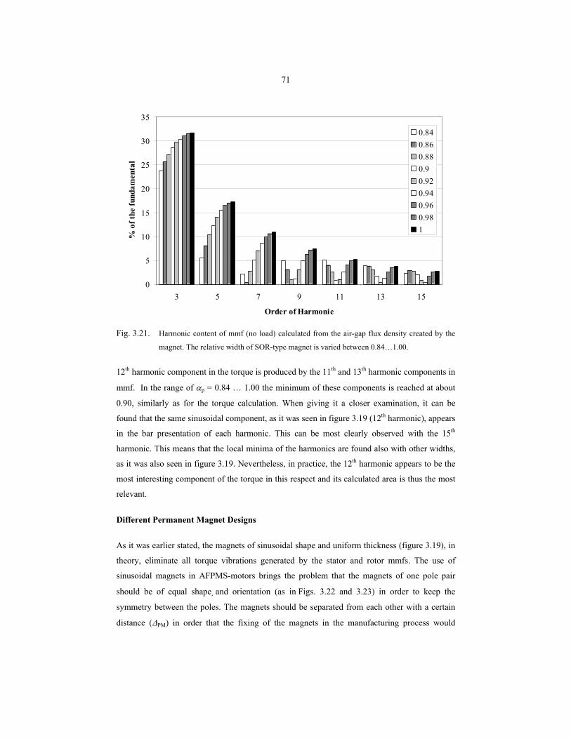
71
0
5
10
15
20
25
30
35
3 5 7 9 11 13 15
Order of Harmonic
% o
f the
fund
amen
tal
0.840.860.880.90.920.940.960.981
Fig. 3.21. Harmonic content of mmf (no load) calculated from the air-gap flux density created by the
magnet. The relative width of SOR-type magnet is varied between 0.84…1.00.
12th harmonic component in the torque is produced by the 11th and 13th harmonic components in
mmf. In the range of αp = 0.84 … 1.00 the minimum of these components is reached at about
0.90, similarly as for the torque calculation. When giving it a closer examination, it can be
found that the same sinusoidal component, as it was seen in figure 3.19 (12th harmonic), appears
in the bar presentation of each harmonic. This can be most clearly observed with the 15th
harmonic. This means that the local minima of the harmonics are found also with other widths,
as it was also seen in figure 3.19. Nevertheless, in practice, the 12th harmonic appears to be the
most interesting component of the torque in this respect and its calculated area is thus the most
relevant.
Different Permanent Magnet Designs
As it was earlier stated, the magnets of sinusoidal shape and uniform thickness (figure 3.19), in
theory, eliminate all torque vibrations generated by the stator and rotor mmfs. The use of
sinusoidal magnets in AFPMS-motors brings the problem that the magnets of one pole pair
should be of equal shape and orientation (as in Figs. 3.22 and 3.23) in order to keep the
symmetry between the poles. The magnets should be separated from each other with a certain
distance (∆PM) in order that the fixing of the magnets in the manufacturing process would
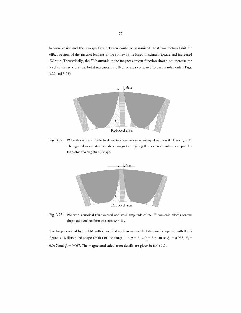
72
become easier and the leakage flux between could be minimized. Last two factors limit the
effective area of the magnet leading in the somewhat reduced maximum torque and increased
T/I ratio. Theoretically, the 3rd harmonic in the magnet contour function should not increase the
level of torque vibration, but it increases the effective area compared to pure fundamental (Figs.
3.22 and 3.23).
∆PM
Reduced area
Fig. 3.22. PM with sinusoidal (only fundamental) contour shape and equal uniform thickness (q = 1).
The figure demonstrates the reduced magnet area giving thus a reduced volume compared to
the sector of a ring (SOR) shape.
∆PM
Reduced area
Fig. 3.23. PM with sinusoidal (fundamental and small amplitude of the 3rd harmonic added) contour
shape and equal uniform thickness (q = 1) .
The torque created by the PM with sinusoidal contour were calculated and compared with the in
figure 3.18 illustrated shape (SOR) of the magnet in q = 2, w/τp= 5/6 stator ξ1 = 0.933, ξ5 =
0.067 and ξ7 = 0.067. The magnet and calculation details are given in table 3.3.
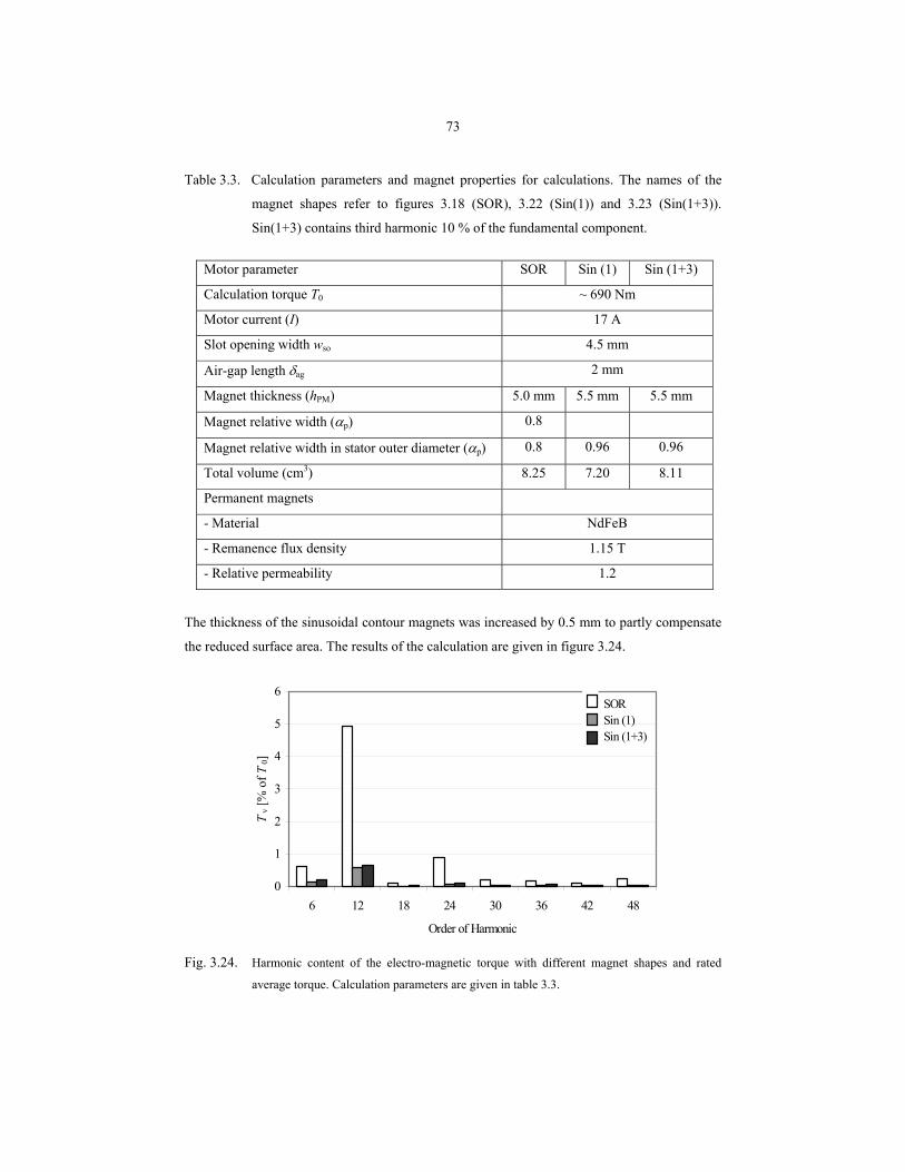
73
Table 3.3. Calculation parameters and magnet properties for calculations. The names of the
magnet shapes refer to figures 3.18 (SOR), 3.22 (Sin(1)) and 3.23 (Sin(1+3)).
Sin(1+3) contains third harmonic 10 % of the fundamental component.
Motor parameter SOR Sin (1) Sin (1+3)
Calculation torque T0 ~ 690 Nm
Motor current (I) 17 A
Slot opening width wso 4.5 mm
Air-gap length δag 2 mm
Magnet thickness (hPM) 5.0 mm 5.5 mm 5.5 mm
Magnet relative width (αp) 0.8
Magnet relative width in stator outer diameter (αp) 0.8 0.96 0.96
Total volume (cm3) 8.25 7.20 8.11
Permanent magnets
- Material NdFeB
- Remanence flux density 1.15 T
- Relative permeability 1.2
The thickness of the sinusoidal contour magnets was increased by 0.5 mm to partly compensate
the reduced surface area. The results of the calculation are given in figure 3.24.
0
1
2
3
4
5
6
6 12 18 24 30 36 42 48
Order of Harmonic
Tv [
% o
f T0]
SORSin (1)Sin (1+3)
Fig. 3.24. Harmonic content of the electro-magnetic torque with different magnet shapes and rated
average torque. Calculation parameters are given in table 3.3.
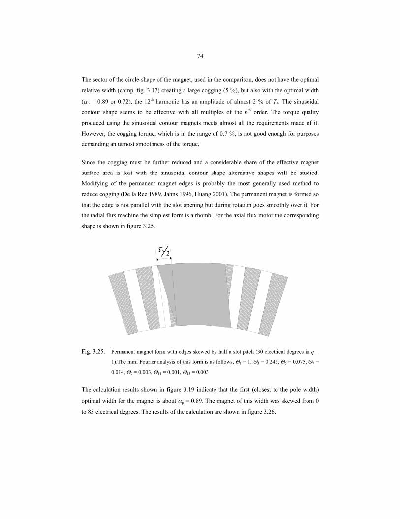
74
The sector of the circle-shape of the magnet, used in the comparison, does not have the optimal
relative width (comp. fig. 3.17) creating a large cogging (5 %), but also with the optimal width
(αp = 0.89 or 0.72), the 12th harmonic has an amplitude of almost 2 % of T0. The sinusoidal
contour shape seems to be effective with all multiples of the 6th order. The torque quality
produced using the sinusoidal contour magnets meets almost all the requirements made of it.
However, the cogging torque, which is in the range of 0.7 %, is not good enough for purposes
demanding an utmost smoothness of the torque.
Since the cogging must be further reduced and a considerable share of the effective magnet
surface area is lost with the sinusoidal contour shape alternative shapes will be studied.
Modifying of the permanent magnet edges is probably the most generally used method to
reduce cogging (De la Ree 1989, Jahns 1996, Huang 2001). The permanent magnet is formed so
that the edge is not parallel with the slot opening but during rotation goes smoothly over it. For
the radial flux machine the simplest form is a rhomb. For the axial flux motor the corresponding
shape is shown in figure 3.25.
sτ 2
Fig. 3.25. Permanent magnet form with edges skewed by half a slot pitch (30 electrical degrees in q =
1).The mmf Fourier analysis of this form is as follows, Θ1 = 1, Θ3 = 0.245, Θ5 = 0.075, Θ7 =
0.014, Θ9 = 0.003, Θ11 = 0.001, Θ13 = 0.003
The calculation results shown in figure 3.19 indicate that the first (closest to the pole width)
optimal width for the magnet is about αp = 0.89. The magnet of this width was skewed from 0
to 85 electrical degrees. The results of the calculation are shown in figure 3.26.
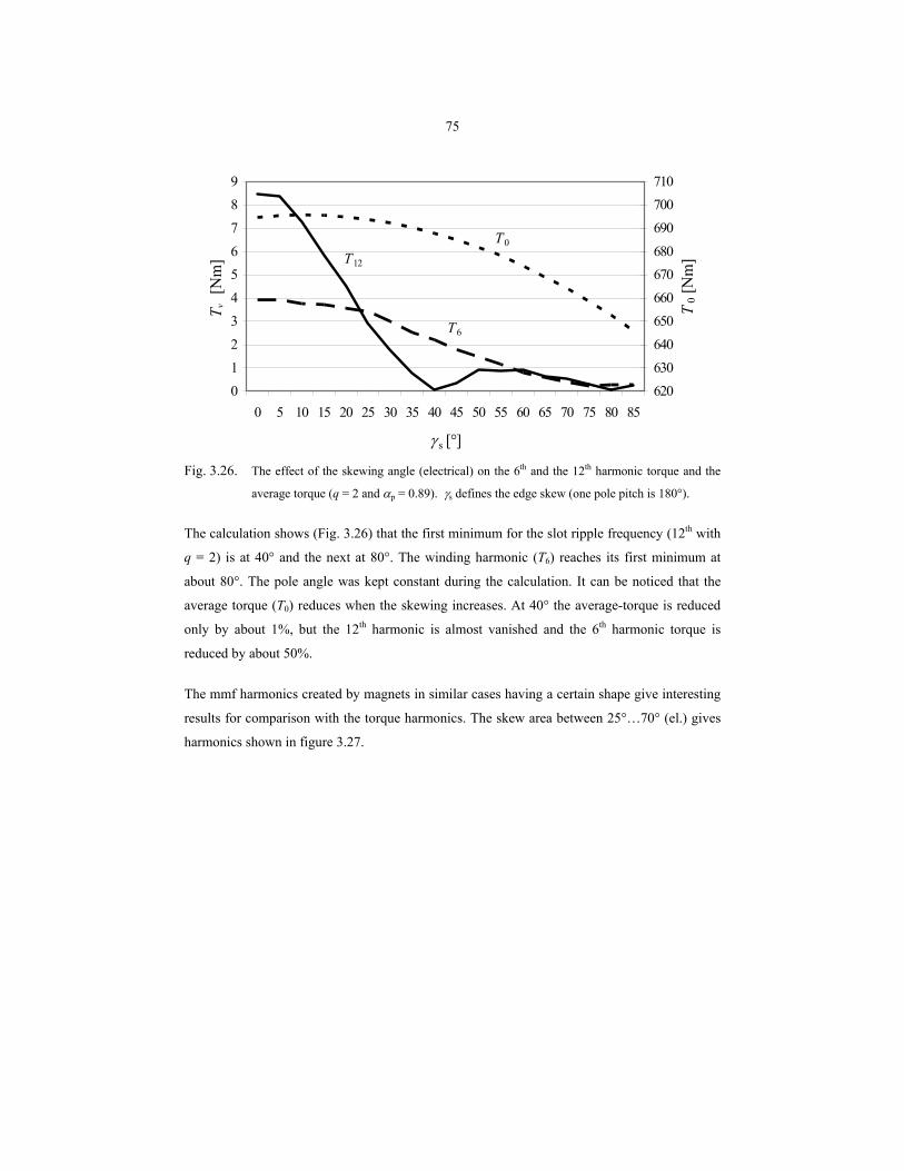
75
0123456789
0 5 10 15 20 25 30 35 40 45 50 55 60 65 70 75 80 85
γ s [°]
T v [
Nm
]
620630640650660670680690700710
T0 [
Nm
]
T0
T12
T6
Fig. 3.26. The effect of the skewing angle (electrical) on the 6th and the 12th harmonic torque and the
average torque (q = 2 and αp = 0.89). γs defines the edge skew (one pole pitch is 180°).
The calculation shows (Fig. 3.26) that the first minimum for the slot ripple frequency (12th with
q = 2) is at 40° and the next at 80°. The winding harmonic (T6) reaches its first minimum at
about 80°. The pole angle was kept constant during the calculation. It can be noticed that the
average torque (T0) reduces when the skewing increases. At 40° the average-torque is reduced
only by about 1%, but the 12th harmonic is almost vanished and the 6th harmonic torque is
reduced by about 50%.
The mmf harmonics created by magnets in similar cases having a certain shape give interesting
results for comparison with the torque harmonics. The skew area between 25°…70° (el.) gives
harmonics shown in figure 3.27.
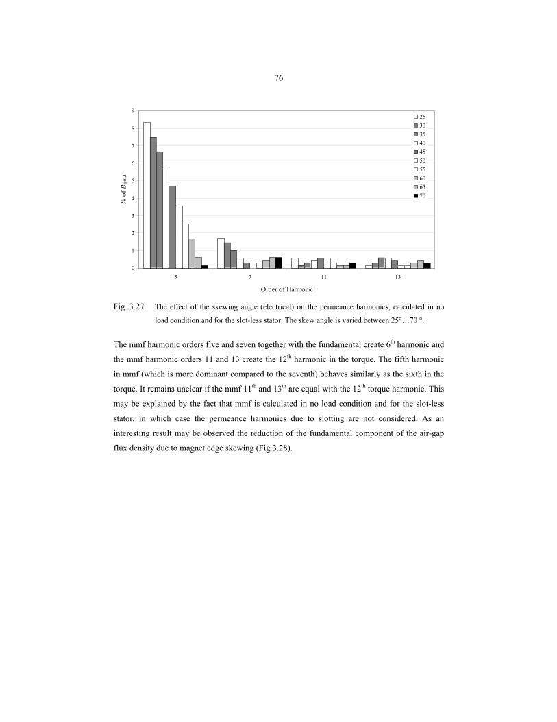
76
0
1
2
3
4
5
6
7
8
9
5 7 11 13
Order of Harmonic
% o
f Bpm
,125303540455055606570
Fig. 3.27. The effect of the skewing angle (electrical) on the permeance harmonics, calculated in no
load condition and for the slot-less stator. The skew angle is varied between 25°…70 °.
The mmf harmonic orders five and seven together with the fundamental create 6th harmonic and
the mmf harmonic orders 11 and 13 create the 12th harmonic in the torque. The fifth harmonic
in mmf (which is more dominant compared to the seventh) behaves similarly as the sixth in the
torque. It remains unclear if the mmf 11th and 13th are equal with the 12th torque harmonic. This
may be explained by the fact that mmf is calculated in no load condition and for the slot-less
stator, in which case the permeance harmonics due to slotting are not considered. As an
interesting result may be observed the reduction of the fundamental component of the air-gap
flux density due to magnet edge skewing (Fig 3.28).
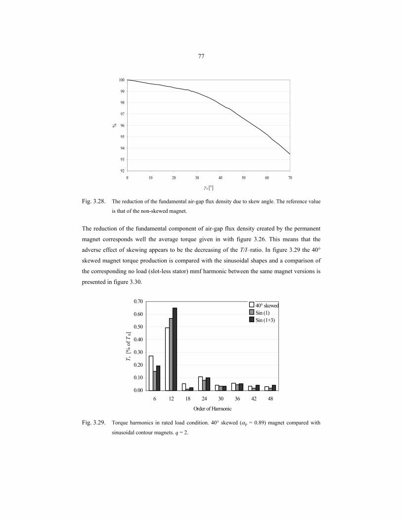
77
92
93
94
95
96
97
98
99
100
0 10 20 30 40 50 60 70
γ s [°]
%
Fig. 3.28. The reduction of the fundamental air-gap flux density due to skew angle. The reference value
is that of the non-skewed magnet.
The reduction of the fundamental component of air-gap flux density created by the permanent
magnet corresponds well the average torque given in with figure 3.26. This means that the
adverse effect of skewing appears to be the decreasing of the T/I–ratio. In figure 3.29 the 40°
skewed magnet torque production is compared with the sinusoidal shapes and a comparison of
the corresponding no load (slot-less stator) mmf harmonic between the same magnet versions is
presented in figure 3.30.
0.00
0.10
0.20
0.30
0.40
0.50
0.60
0.70
6 12 18 24 30 36 42 48
Order of Harmonic
T v [%
of T
0]
40° skewedSin (1)Sin (1+3)
Fig. 3.29. Torque harmonics in rated load condition. 40° skewed (αp = 0.89) magnet compared with
sinusoidal contour magnets. q = 2.
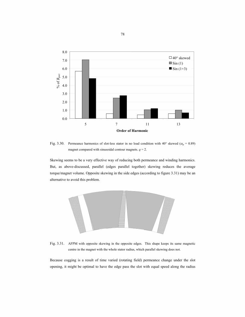
78
Fig. 3.30. Permeance harmonics of slot-less stator in no load condition with 40° skewed (αp = 0.89)
magnet compared with sinusoidal contour magnets. q = 2.
Skewing seems to be a very effective way of reducing both permeance and winding harmonics.
But, as above-discussed, parallel (edges parallel together) skewing reduces the average
torque/magnet volume. Opposite skewing in the side edges (according to figure 3.31) may be an
alternative to avoid this problem.
Fig. 3.31. AFPM with opposite skewing in the opposite edges. This shape keeps its same magnetic
centre in the magnet with the whole stator radius, which parallel skewing does not.
Because cogging is a result of time varied (rotating field) permeance change under the slot
opening, it might be optimal to have the edge pass the slot with equal speed along the radius
0.0
1.0
2.0
3.0
4.0
5.0
6.0
7.0
8.0
5 7 11 13
Order of Harmonic
% o
f Bpm
1 40° skewed Sin (1) Sin (1+3)
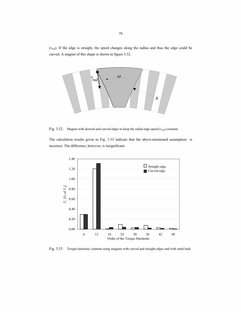
79
(vrad). If the edge is straight, the speed changes along the radius and thus the edge could be
curved. A magnet of this shape is shown in figure 3.32.
vradω
R
Fig. 3.32. Magnet with skewed and curved edges to keep the radial edge speed (vrad) constant.
The calculation results given in Fig. 3.33 indicate that the above-mentioned assumption is
incorrect. The difference, however, is insignificant.
0.00
0.20
0.40
0.60
0.80
1.00
1.20
1.40
6 12 18 24 30 36 42 48Order of the Torque Harmonic
T v [%
of T
0]
Straight edgeCurved edge
Fig. 3.33. Torque harmonic contents using magnets with curved and straight edges and with rated load.
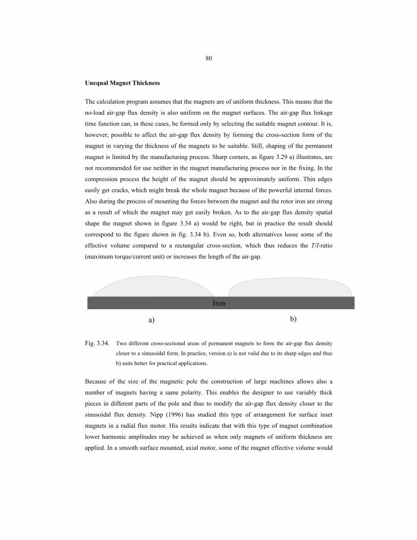
80
Unequal Magnet Thickness
The calculation program assumes that the magnets are of uniform thickness. This means that the
no-load air-gap flux density is also uniform on the magnet surfaces. The air-gap flux linkage
time function can, in these cases, be formed only by selecting the suitable magnet contour. It is,
however, possible to affect the air-gap flux density by forming the cross-section form of the
magnet in varying the thickness of the magnets to be suitable. Still, shaping of the permanent
magnet is limited by the manufacturing process. Sharp corners, as figure 3.29 a) illustrates, are
not recommended for use neither in the magnet manufacturing process nor in the fixing. In the
compression process the height of the magnet should be approximately uniform. Thin edges
easily get cracks, which might break the whole magnet because of the powerful internal forces.
Also during the process of mounting the forces between the magnet and the rotor iron are strong
as a result of which the magnet may get easily broken. As to the air-gap flux density spatial
shape the magnet shown in figure 3.34 a) would be right, but in practice the result should
correspond to the figure shown in fig. 3.34 b). Even so, both alternatives loose some of the
effective volume compared to a rectangular cross-section, which thus reduces the T/I-ratio
(maximum torque/current unit) or increases the length of the air-gap.
a) b)
Iron
Fig. 3.34. Two different cross-sectional areas of permanent magnets to form the air-gap flux density
closer to a sinusoidal form. In practice, version a) is not valid due to its sharp edges and thus
b) suits better for practical applications.
Because of the size of the magnetic pole the construction of large machines allows also a
number of magnets having a same polarity. This enables the designer to use variably thick
pieces in different parts of the pole and thus to modify the air-gap flux density closer to the
sinusoidal flux density. Nipp (1996) has studied this type of arrangement for surface inset
magnets in a radial flux motor. His results indicate that with this type of magnet combination
lower harmonic amplitudes may be achieved as when only magnets of uniform thickness are
applied. In a smooth surface mounted, axial motor, some of the magnet effective volume would
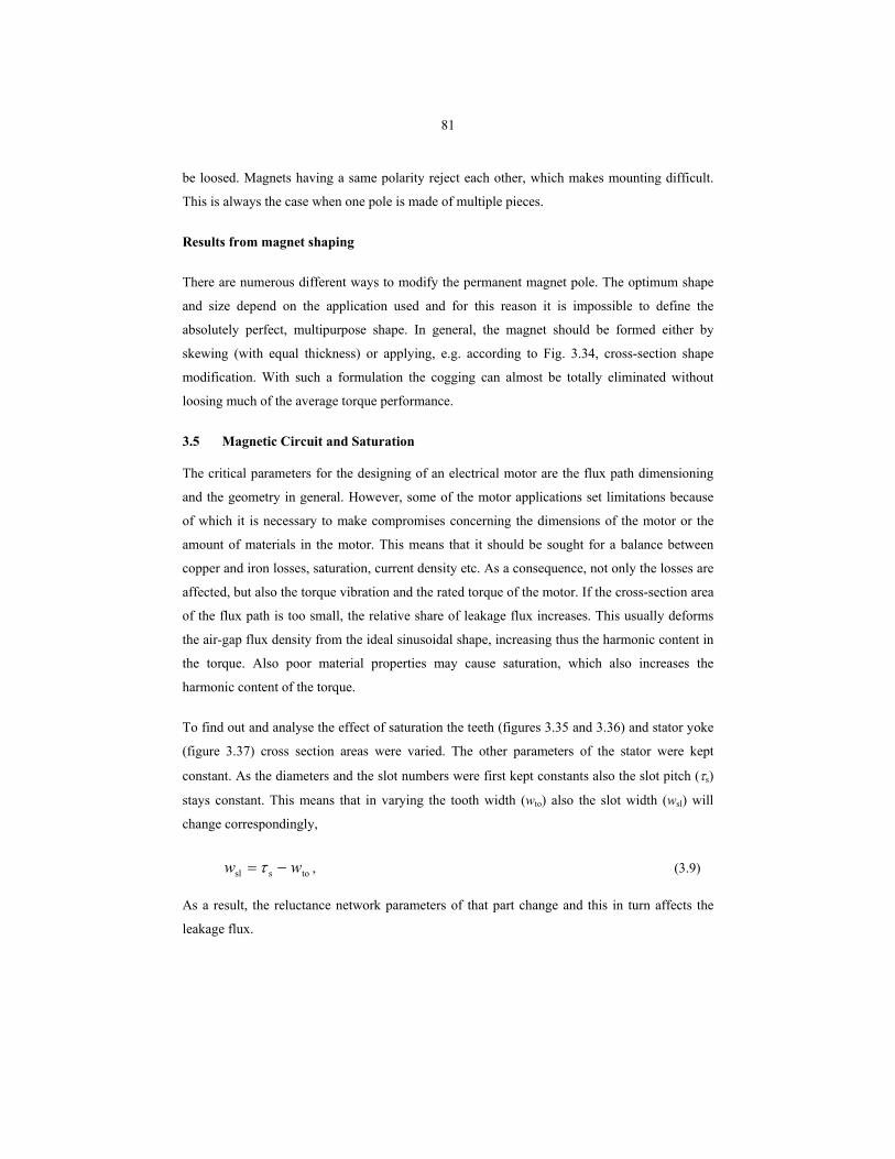
81
be loosed. Magnets having a same polarity reject each other, which makes mounting difficult.
This is always the case when one pole is made of multiple pieces.
Results from magnet shaping
There are numerous different ways to modify the permanent magnet pole. The optimum shape
and size depend on the application used and for this reason it is impossible to define the
absolutely perfect, multipurpose shape. In general, the magnet should be formed either by
skewing (with equal thickness) or applying, e.g. according to Fig. 3.34, cross-section shape
modification. With such a formulation the cogging can almost be totally eliminated without
loosing much of the average torque performance.
3.5 Magnetic Circuit and Saturation
The critical parameters for the designing of an electrical motor are the flux path dimensioning
and the geometry in general. However, some of the motor applications set limitations because
of which it is necessary to make compromises concerning the dimensions of the motor or the
amount of materials in the motor. This means that it should be sought for a balance between
copper and iron losses, saturation, current density etc. As a consequence, not only the losses are
affected, but also the torque vibration and the rated torque of the motor. If the cross-section area
of the flux path is too small, the relative share of leakage flux increases. This usually deforms
the air-gap flux density from the ideal sinusoidal shape, increasing thus the harmonic content in
the torque. Also poor material properties may cause saturation, which also increases the
harmonic content of the torque.
To find out and analyse the effect of saturation the teeth (figures 3.35 and 3.36) and stator yoke
(figure 3.37) cross section areas were varied. The other parameters of the stator were kept
constant. As the diameters and the slot numbers were first kept constants also the slot pitch (τs)
stays constant. This means that in varying the tooth width (wto) also the slot width (wsl) will
change correspondingly,
tossl ww −= τ , (3.9)
As a result, the reluctance network parameters of that part change and this in turn affects the
leakage flux.
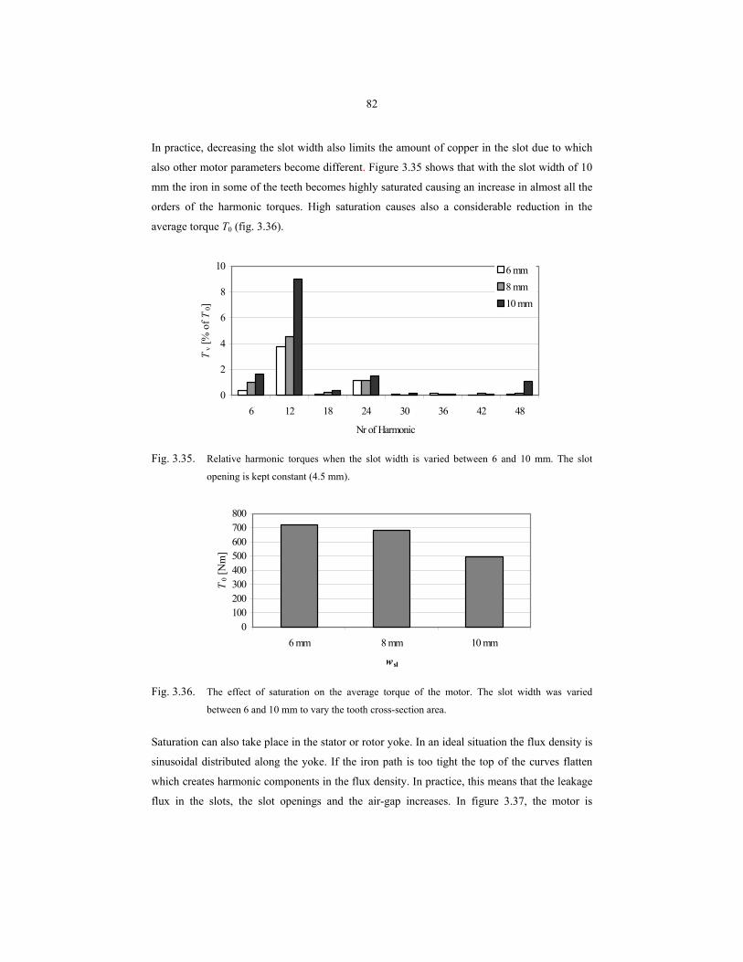
82
In practice, decreasing the slot width also limits the amount of copper in the slot due to which
also other motor parameters become different. Figure 3.35 shows that with the slot width of 10
mm the iron in some of the teeth becomes highly saturated causing an increase in almost all the
orders of the harmonic torques. High saturation causes also a considerable reduction in the
average torque T0 (fig. 3.36).
0
2
4
6
8
10
6 12 18 24 30 36 42 48
Nr of Harmonic
Tv [
% o
f T0]
6 mm8 mm10 mm
Fig. 3.35. Relative harmonic torques when the slot width is varied between 6 and 10 mm. The slot
opening is kept constant (4.5 mm).
0100200300400500600700800
6 mm 8 mm 10 mm
wsl
T0 [
Nm
]
Fig. 3.36. The effect of saturation on the average torque of the motor. The slot width was varied
between 6 and 10 mm to vary the tooth cross-section area.
Saturation can also take place in the stator or rotor yoke. In an ideal situation the flux density is
sinusoidal distributed along the yoke. If the iron path is too tight the top of the curves flatten
which creates harmonic components in the flux density. In practice, this means that the leakage
flux in the slots, the slot openings and the air-gap increases. In figure 3.37, the motor is
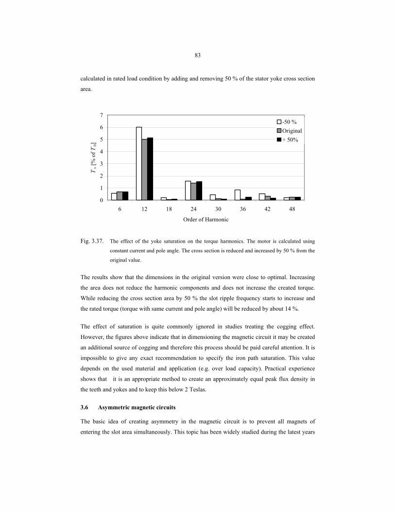
83
calculated in rated load condition by adding and removing 50 % of the stator yoke cross section
area.
0
1
2
3
4
5
6
7
6 12 18 24 30 36 42 48
Order of Harmonic
Tv [
% o
f T0]
-50 %Original+ 50%
Fig. 3.37. The effect of the yoke saturation on the torque harmonics. The motor is calculated using
constant current and pole angle. The cross section is reduced and increased by 50 % from the
original value.
The results show that the dimensions in the original version were close to optimal. Increasing
the area does not reduce the harmonic components and does not increase the created torque.
While reducing the cross section area by 50 % the slot ripple frequency starts to increase and
the rated torque (torque with same current and pole angle) will be reduced by about 14 %.
The effect of saturation is quite commonly ignored in studies treating the cogging effect.
However, the figures above indicate that in dimensioning the magnetic circuit it may be created
an additional source of cogging and therefore this process should be paid careful attention. It is
impossible to give any exact recommendation to specify the iron path saturation. This value
depends on the used material and application (e.g. over load capacity). Practical experience
shows that it is an appropriate method to create an approximately equal peak flux density in
the teeth and yokes and to keep this below 2 Teslas.
3.6 Asymmetric magnetic circuits
The basic idea of creating asymmetry in the magnetic circuit is to prevent all magnets of
entering the slot area simultaneously. This topic has been widely studied during the latest years
84
(Studer 1997, Zhu 2000 and Bianchi 2000). In symmetric permanent magnet distribution all
poles amplify the harmonic frequencies in the same phase angle. In ideal asymmetry the same
excitation exists in each pole as it does in the symmetric distribution, but because the phase
angles are different in the slot frequencies the poles compensate each other. The slot frequency
(cogging) is defined as
ss qmff
pQf 2sf == , (3.10)
where q is the number of slots per pole and phase, m is the number of phases and fs is the supply
frequency.
Asymmetry has also its disadvantages. Depending on the type and degree of asymmetry low
order harmonics such as first or second or even sub-harmonics, which in symmetric cases with
no offset or gain error do not exist, may appear.
This may be due to the fact that the phase angle between the coils or of the fundamental wave
of the linear current distribution is unequal, or the leakage fluxes in different poles differ from
each other. The asymmetric magnetic circuit also causes asymmetry in the reluctance network
due to different cross section areas or permeability of the corresponding parts of the magnetic
circuit. This means that the electro-motive forces in different poles are in a different angle, as a
result of which asymmetry occurs in the magnetic circuits between the poles, which affects the
saturation of the circuit and the multiphase electric circuit. In series connected circuits this
effect is more controllable due to equal current in each of the phase coils. Also the EMF is the
sum of individual coils. When there are several branches, asymmetry caused by the unequal
current distribution may change the balance between these branches causing thus saturation and
flux differences in the magnetic circuit.
In case of symmetric magnetic circuit every pole may be put to work in the optimum point to
maximize the T/I -ratio or just the torque. When the torque versus pole angle is sinusoidal and
not linear, the T/I –ratio is, compared to a symmetric circuit, always somewhat smaller. The
extreme case is when the asymmetry is increased equally to 180 electric decrees. In this case the
sum torque is always zero, even though individual poles create torque.
85
To decrease the cogging torque the asymmetry needed is from zero to one slot pitch. The bigger
the slot number per pole and phase q is set, the smaller the angle of one slot pitch is obtained
and also the smaller the required relative asymmetry will be compared to the pole width.
The more complex the asymmetry appears to be, the more difficult the model for calculation
will be. In practice, asymmetry brings that the whole machine has to be calculated instead of
just one pole pair. In many cases FEM offers the easiest way of calculating.
The following chapters studies different possibilities of creating asymmetry in the magnetic
circuit.
3.6.1 Asymmetric Magnet Distribution
It may be consequently assumed that when all the magnet edges, where the derivative
component of the magnet flux density is at its highest, enter the slot openings at the same time
high cogging torque is created. The cogging torque is usually reduced by forming the magnet
edges so that these are not parallel to the stator slots. The shape of the air-gap flux linkage
becomes thus closer to sinusoidal. But also in this case, all the non-linearities meet the slots
simultaneously and this causes cogging.
In addition to the option of forming the geometry of the magnets, it is also possible to place
them somewhat asymmetric on the rotor surface (fig. 3.38). An asymmetric distribution can be
created in many different ways. All the magnets can be put in different deflection from the
symmetrical centre point or they can be for example shifted in pairs. However, some factors
limiting deflection should be considered. Firstly, the magnets cannot overlap. Deflection is, in
this case, defined by the magnet shape and the relative width compared to the pole. The other
reason is that shifting the poles limits the maximum torque of the motor. If the edges of adjacent
magnets are very close to each other the leakage flux from one pole to the other increases due to
which the air-gap magnetization decreases.
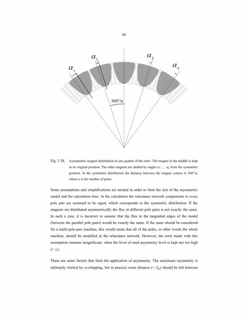
86
α1
α2α3
α4
360°/n
Fig. 3.38. Asymmetric magnet distribution in one quarter of the rotor. The magnet in the middle is kept
in its original position. The other magnets are shifted by angles α1 … α4 from the symmetric
position. In the symmetric distribution the distance between the magnet centres is 360°/n,
where n is the number of poles.
Some assumptions and simplifications are needed in order to limit the size of the asymmetric
model and the calculation time. In the calculation the reluctance network components in every
pole pair are assumed to be equal, which corresponds to the symmetric distribution. If the
magnets are distributed asymmetrically the flux in different pole pairs is not exactly the same.
In such a case, it is incorrect to assume that the flux in the tangential edges of the model
(between the parallel pole pairs) would be exactly the same. If the same should be considered
for a multi-pole-pair machine, this would mean that all of the poles, in other words the whole
machine, should be modelled in the reluctance network. However, the error made with this
assumption remains insignificant, when the level of used asymmetry level is kept not too high
(> τs).
There are some factors that limit the application of asymmetry. The maximum asymmetry is
ultimately limited by overlapping, but in practice some distance (> δag) should be left between
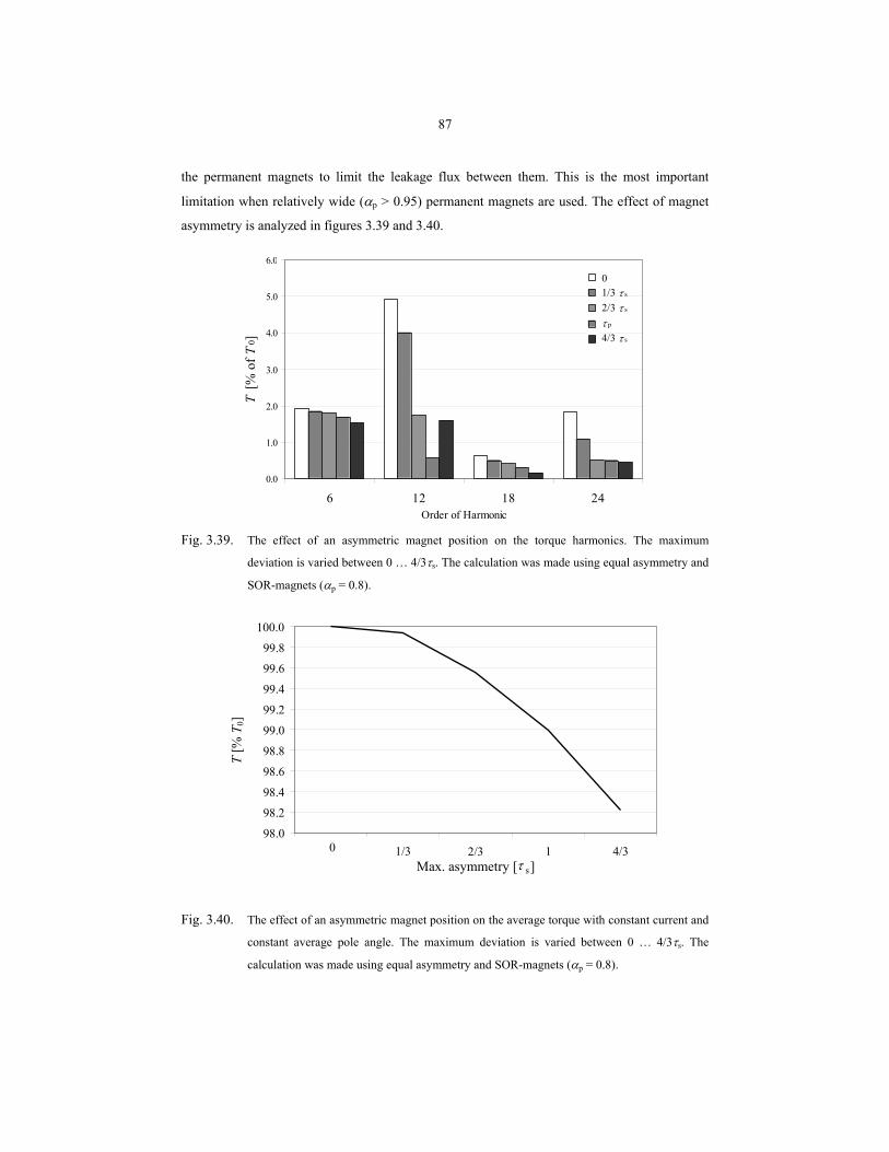
87
the permanent magnets to limit the leakage flux between them. This is the most important
limitation when relatively wide (αp > 0.95) permanent magnets are used. The effect of magnet
asymmetry is analyzed in figures 3.39 and 3.40.
0.0
1.0
2.0
3.0
4.0
5.0
6.0
6 12 18 24Order of Harmonic
T [%
of T
0 ]
01/3 τ s
2/3 τ s
τ p
4/3 τ s
Fig. 3.39. The effect of an asymmetric magnet position on the torque harmonics. The maximum
deviation is varied between 0 … 4/3τs. The calculation was made using equal asymmetry and
SOR-magnets (αp = 0.8).
Fig. 3.40. The effect of an asymmetric magnet position on the average torque with constant current and
constant average pole angle. The maximum deviation is varied between 0 … 4/3τs. The
calculation was made using equal asymmetry and SOR-magnets (αp = 0.8).
98.0
98.2
98.4
98.6
98.8
99.0
99.2
99.4
99.6
99.8
100.0
0 1/3 2/3 1 4/3 Max. asymmetry [τ s ]
T [%
T0]
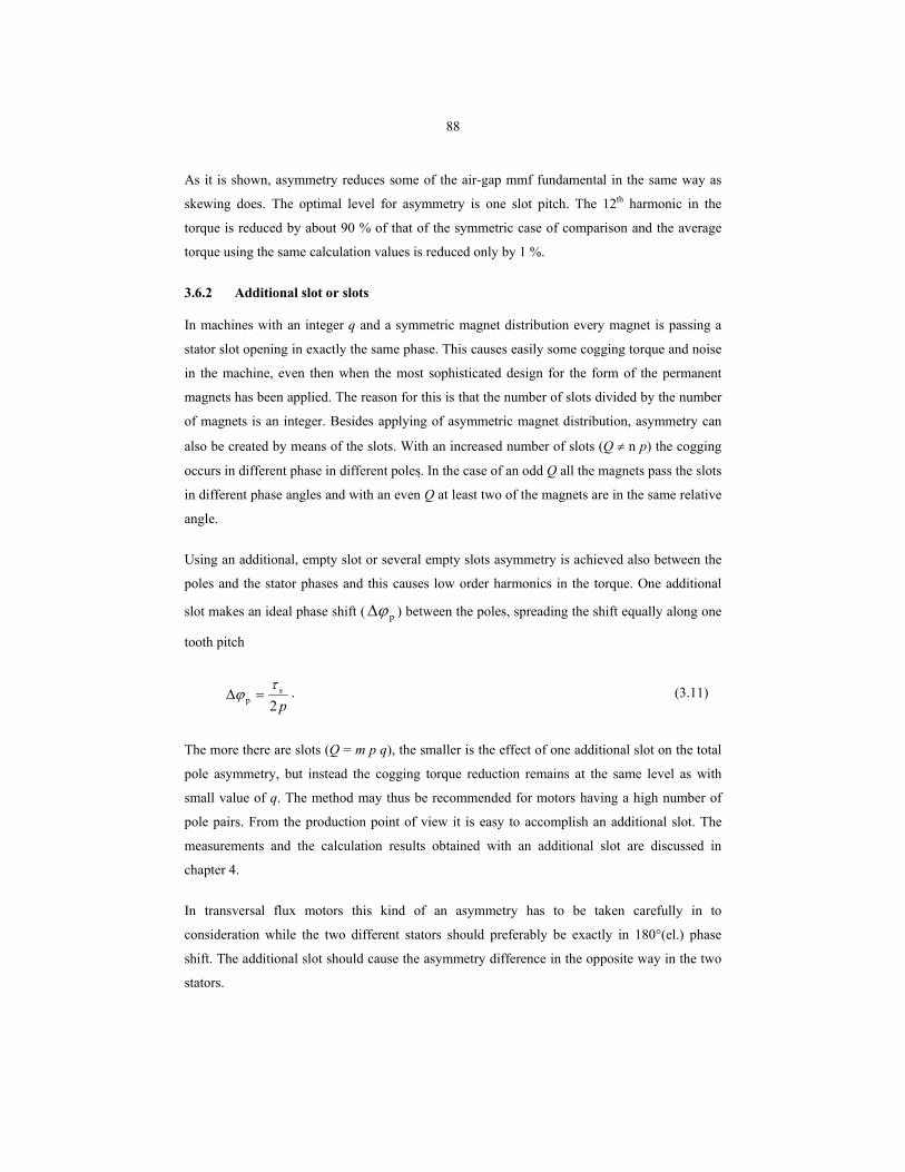
88
As it is shown, asymmetry reduces some of the air-gap mmf fundamental in the same way as
skewing does. The optimal level for asymmetry is one slot pitch. The 12th harmonic in the
torque is reduced by about 90 % of that of the symmetric case of comparison and the average
torque using the same calculation values is reduced only by 1 %.
3.6.2 Additional slot or slots
In machines with an integer q and a symmetric magnet distribution every magnet is passing a
stator slot opening in exactly the same phase. This causes easily some cogging torque and noise
in the machine, even then when the most sophisticated design for the form of the permanent
magnets has been applied. The reason for this is that the number of slots divided by the number
of magnets is an integer. Besides applying of asymmetric magnet distribution, asymmetry can
also be created by means of the slots. With an increased number of slots (Q ≠ n p) the cogging
occurs in different phase in different poles. In the case of an odd Q all the magnets pass the slots
in different phase angles and with an even Q at least two of the magnets are in the same relative
angle.
Using an additional, empty slot or several empty slots asymmetry is achieved also between the
poles and the stator phases and this causes low order harmonics in the torque. One additional
slot makes an ideal phase shift ( pϕ∆ ) between the poles, spreading the shift equally along one
tooth pitch
p2s
pτ
ϕ =∆ . (3.11)
The more there are slots (Q = m p q), the smaller is the effect of one additional slot on the total
pole asymmetry, but instead the cogging torque reduction remains at the same level as with
small value of q. The method may thus be recommended for motors having a high number of
pole pairs. From the production point of view it is easy to accomplish an additional slot. The
measurements and the calculation results obtained with an additional slot are discussed in
chapter 4.
In transversal flux motors this kind of an asymmetry has to be taken carefully in to
consideration while the two different stators should preferably be exactly in 180°(el.) phase
shift. The additional slot should cause the asymmetry difference in the opposite way in the two
stators.
89
3.6.3 Eccentricity
Eccentricity is one of the factors that create unwished harmonic torques in the motors. This
subject has been studied by e.g. Kim 1998, Wang 1999 and Paljan 2000. Eccentricity appears to
be a problem in radial motors, more precisely in cases where the rotor alignment in the
manufacturing process did not succeed or the rotor stiffness is not sufficient. However,
eccentricity is more an unpredictable error of manufacturing, not a designing criterion, and is
therefore not treated in detail in this research. Furthermore, it would require a different way of
handling the air-gap reluctances and flux density created by the magnets to study eccentricity
using the calculation method presented in chapter 2.
3.7 Conclusions
It is shown that in forming the magnet and using asymmetry either in the stator or magnet
distribution it is possible to effectively reduce the cogging torque without dramatically affecting
the torque average value. The winding arrangements and number of slots per pole and phase are
a means of reducing the winding harmonics. Since the magnetic circuit depends on different
factors as e.g. application, its requirements, manufacturing capabilities and other elements like
the cost target of the machine, it is impossible to recommend any exact design for it. However,
it may be stated that, generally, forming the magnet and using suitable asymmetry should be
recommendable in most of the cases.
90
4 MODEL VERIFICATION – EXPERIMENTAL RESULTS
According to the calculations discussed in chapters 2 and 3 there exist many possibilities to
affect the torque ripple of a permanent magnet synchronous motor. The results are based on
theoretical studies and it is the objective of this chapter to show that the calculated and
measured values correspond well to each other. It is also shown that based on the principles
obtained with the calculation model introduced in this work it is possible to produce a really
low torque ripple machine.
4.1 Reference Motor Versions
The motors manufactured to perform verification are axial flux motors with Qs = 120, q = 2,
w/τp = 5/6 and p = 10, which is a motor configuration that produces a fairly low amount of
stator harmonic magneto-motive force components. The elimination of the cogging torque is
thus emphasized when the designing is made for the purpose of achieving a smooth torque. The
calculation program enables the use of rotor PM of almost arbitrary shapes. Only the magnet
width is restricted to be less than or equal with the pole pitch (αp ≤ 1). Based on the
calculations results three different magnet shapes were selected for practical verification of the
results. The selected magnets shapes are illustrated in figure 4.1. The magnet shape shown in
Fig. 4.1 a is optimised to achieve the lowest possible cogging. With the sinusoidal magnet shape
(Fig. 4.1 b) no stator winding harmonics based torque components are produced since this shape
produces a flux linkage containing only the first and the third harmonic. The magnet contour
shape shown in Fig. 4.1 c is close to that of a sinusoidal magnet which has a negative third
amplitude. The stator slot passing velocity of the magnet edges is almost constant and thus the
cogging will remain low. In this study the magnets will be further called respectively: a) PM1x,
b) PM2 and c) PM3x, where the subscript x indicates the asymmetry level of the magnet
positioning as follows:
- x = 0 symmetric distribution
- x = 1 max. deviation from the symmetry ±7° (electrical)
- x = 2 max. deviation from the symmetry ±14° (el.)
The magnets of the PM1 and PM3 type were mounted symmetrically as well as asymmetrically.
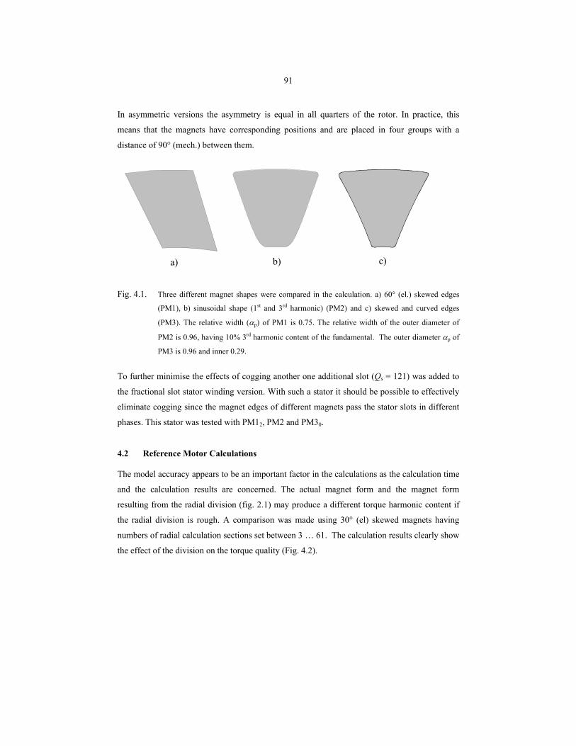
91
In asymmetric versions the asymmetry is equal in all quarters of the rotor. In practice, this
means that the magnets have corresponding positions and are placed in four groups with a
distance of 90° (mech.) between them.
a) b) c)
Fig. 4.1. Three different magnet shapes were compared in the calculation. a) 60° (el.) skewed edges
(PM1), b) sinusoidal shape (1st and 3rd harmonic) (PM2) and c) skewed and curved edges
(PM3). The relative width (αp) of PM1 is 0.75. The relative width of the outer diameter of
PM2 is 0.96, having 10% 3rd harmonic content of the fundamental. The outer diameter αp of
PM3 is 0.96 and inner 0.29.
To further minimise the effects of cogging another one additional slot (Qs = 121) was added to
the fractional slot stator winding version. With such a stator it should be possible to effectively
eliminate cogging since the magnet edges of different magnets pass the stator slots in different
phases. This stator was tested with PM12, PM2 and PM30.
4.2 Reference Motor Calculations
The model accuracy appears to be an important factor in the calculations as the calculation time
and the calculation results are concerned. The actual magnet form and the magnet form
resulting from the radial division (fig. 2.1) may produce a different torque harmonic content if
the radial division is rough. A comparison was made using 30° (el) skewed magnets having
numbers of radial calculation sections set between 3 … 61. The calculation results clearly show
the effect of the division on the torque quality (Fig. 4.2).
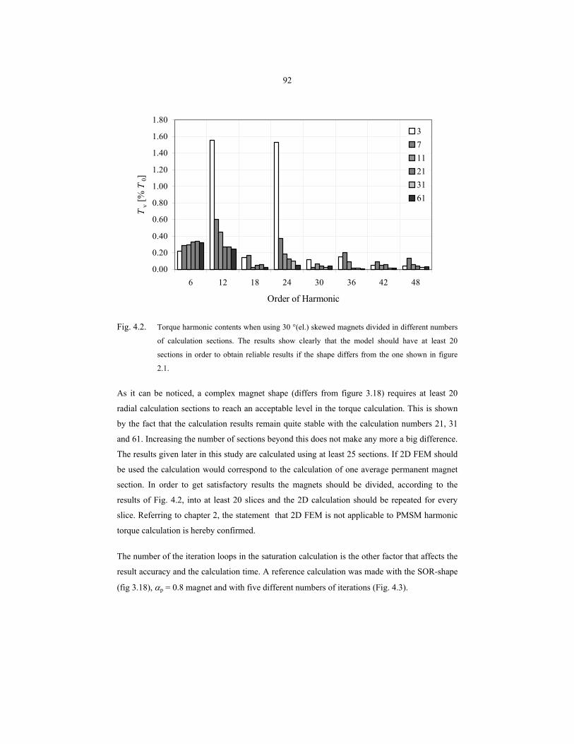
92
0.00
0.20
0.40
0.60
0.80
1.00
1.20
1.40
1.60
1.80
6 12 18 24 30 36 42 48
Order of Harmonic
Tν [
% T
0]3711213161
Fig. 4.2. Torque harmonic contents when using 30 °(el.) skewed magnets divided in different numbers
of calculation sections. The results show clearly that the model should have at least 20
sections in order to obtain reliable results if the shape differs from the one shown in figure
2.1.
As it can be noticed, a complex magnet shape (differs from figure 3.18) requires at least 20
radial calculation sections to reach an acceptable level in the torque calculation. This is shown
by the fact that the calculation results remain quite stable with the calculation numbers 21, 31
and 61. Increasing the number of sections beyond this does not make any more a big difference.
The results given later in this study are calculated using at least 25 sections. If 2D FEM should
be used the calculation would correspond to the calculation of one average permanent magnet
section. In order to get satisfactory results the magnets should be divided, according to the
results of Fig. 4.2, into at least 20 slices and the 2D calculation should be repeated for every
slice. Referring to chapter 2, the statement that 2D FEM is not applicable to PMSM harmonic
torque calculation is hereby confirmed.
The number of the iteration loops in the saturation calculation is the other factor that affects the
result accuracy and the calculation time. A reference calculation was made with the SOR-shape
(fig 3.18), αp = 0.8 magnet and with five different numbers of iterations (Fig. 4.3).
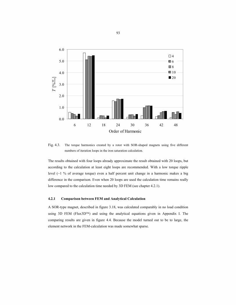
93
0.0
1.0
2.0
3.0
4.0
5.0
6.0
6 12 18 24 30 36 42 48
Order of Harmonic
T [%
T n]
4681020
Fig. 4.3. The torque harmonics created by a rotor with SOR-shaped magnets using five different
numbers of iteration loops in the iron saturation calculation.
The results obtained with four loops already approximate the result obtained with 20 loops, but
according to the calculation at least eight loops are recommended. With a low torque ripple
level (~1 % of average torque) even a half percent unit change in a harmonic makes a big
difference in the comparison. Even when 20 loops are used the calculation time remains really
low compared to the calculation time needed by 3D FEM (see chapter 4.2.1).
4.2.1 Comparison between FEM and Analytical Calculation
A SOR-type magnet, described in figure 3.18, was calculated comparably in no load condition
using 3D FEM (Flux3D) and using the analytical equations given in Appendix I. The
comparing results are given in figure 4.4. Because the model turned out to be to large, the
element network in the FEM-calculation was made somewhat sparse.
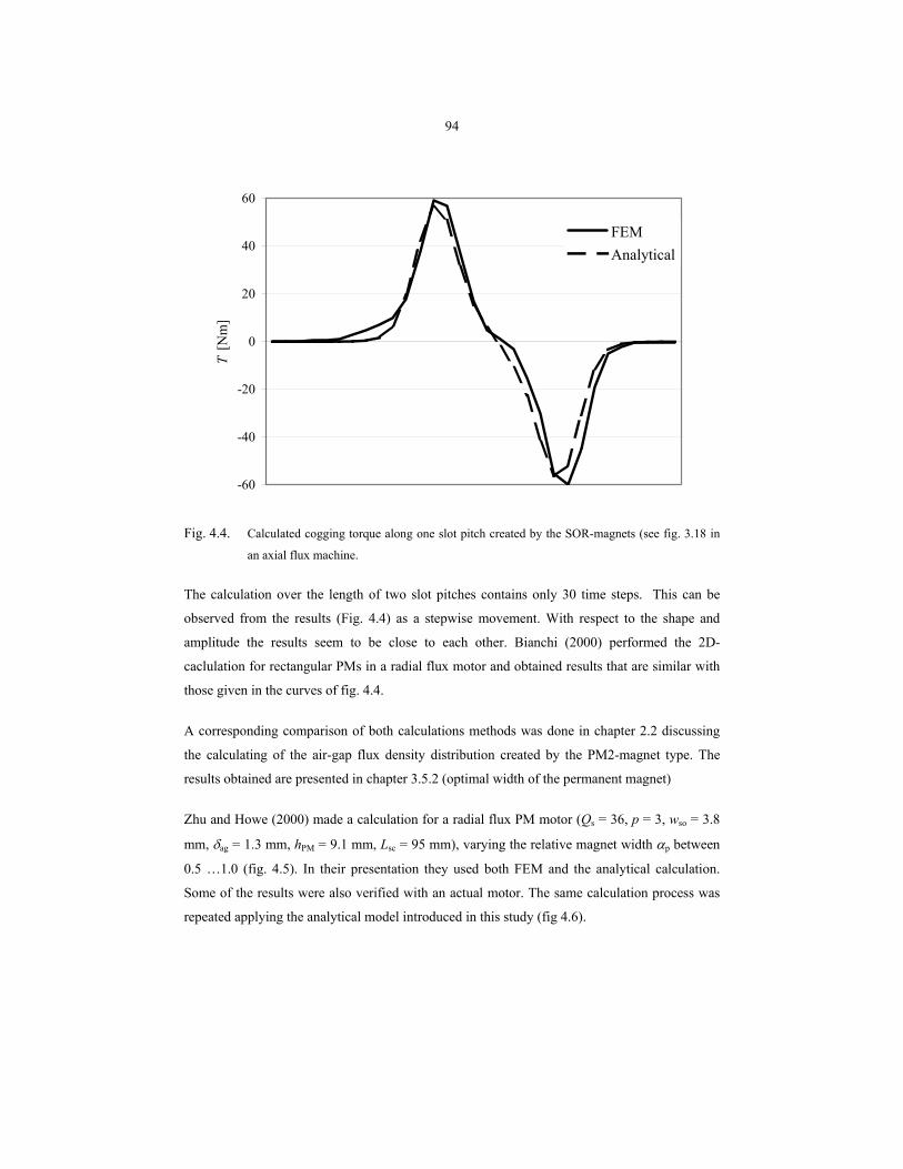
94
-60
-40
-20
0
20
40
60
T [N
m]
FEMAnalytical
Fig. 4.4. Calculated cogging torque along one slot pitch created by the SOR-magnets (see fig. 3.18 in
an axial flux machine.
The calculation over the length of two slot pitches contains only 30 time steps. This can be
observed from the results (Fig. 4.4) as a stepwise movement. With respect to the shape and
amplitude the results seem to be close to each other. Bianchi (2000) performed the 2D-
caclulation for rectangular PMs in a radial flux motor and obtained results that are similar with
those given in the curves of fig. 4.4.
A corresponding comparison of both calculations methods was done in chapter 2.2 discussing
the calculating of the air-gap flux density distribution created by the PM2-magnet type. The
results obtained are presented in chapter 3.5.2 (optimal width of the permanent magnet)
Zhu and Howe (2000) made a calculation for a radial flux PM motor (Qs = 36, p = 3, wso = 3.8
mm, δag = 1.3 mm, hPM = 9.1 mm, Lsc = 95 mm), varying the relative magnet width αp between
0.5 …1.0 (fig. 4.5). In their presentation they used both FEM and the analytical calculation.
Some of the results were also verified with an actual motor. The same calculation process was
repeated applying the analytical model introduced in this study (fig 4.6).
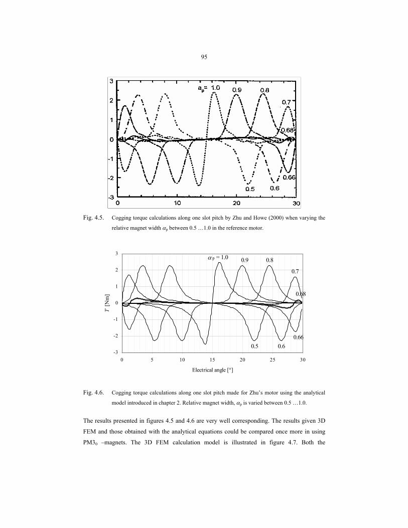
95
Fig. 4.5. Cogging torque calculations along one slot pitch by Zhu and Howe (2000) when varying the
relative magnet width αp between 0.5 …1.0 in the reference motor.
-3
-2
-1
0
1
2
3
0 5 10 15 20 25 30
Electrical angle [°]
T [N
m]
α p = 1.0 0.9 0.8
0.7
0.68
0.66 0.6 0.5
Fig. 4.6. Cogging torque calculations along one slot pitch made for Zhu’s motor using the analytical
model introduced in chapter 2. Relative magnet width, αp is varied between 0.5 …1.0.
The results presented in figures 4.5 and 4.6 are very well corresponding. The results given 3D
FEM and those obtained with the analytical equations could be compared once more in using
PM30 –magnets. The 3D FEM calculation model is illustrated in figure 4.7. Both the
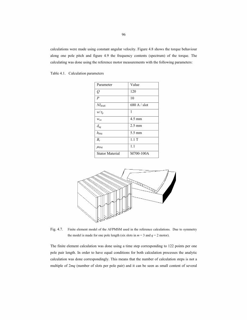
96
calculations were made using constant angular velocity. Figure 4.8 shows the torque behaviour
along one pole pitch and figure 4.9 the frequency contents (spectrum) of the torque. The
calculating was done using the reference motor measurements with the following parameters:
Table 4.1. Calculation parameters
Fig. 4.7. Finite element model of the AFPMSM used in the reference calculations. Due to symmetry
the model is made for one pole length (six slots in m = 3 and q = 2 motor).
The finite element calculation was done using a time step corresponding to 122 points per one
pole pair length. In order to have equal conditions for both calculation processes the analytic
calculation was done correspondingly. This means that the number of calculation steps is not a
multiple of 2mq (number of slots per pole pair) and it can be seen as small content of several
Parameter Value
Q 120
P 10
NIRMS 680 A / slot
w/τp 1
wso 4.5 mm
δag 2.5 mm
hPM 5.5 mm
Br 1.1 T
µPM 1.1
Stator Material M700-100A
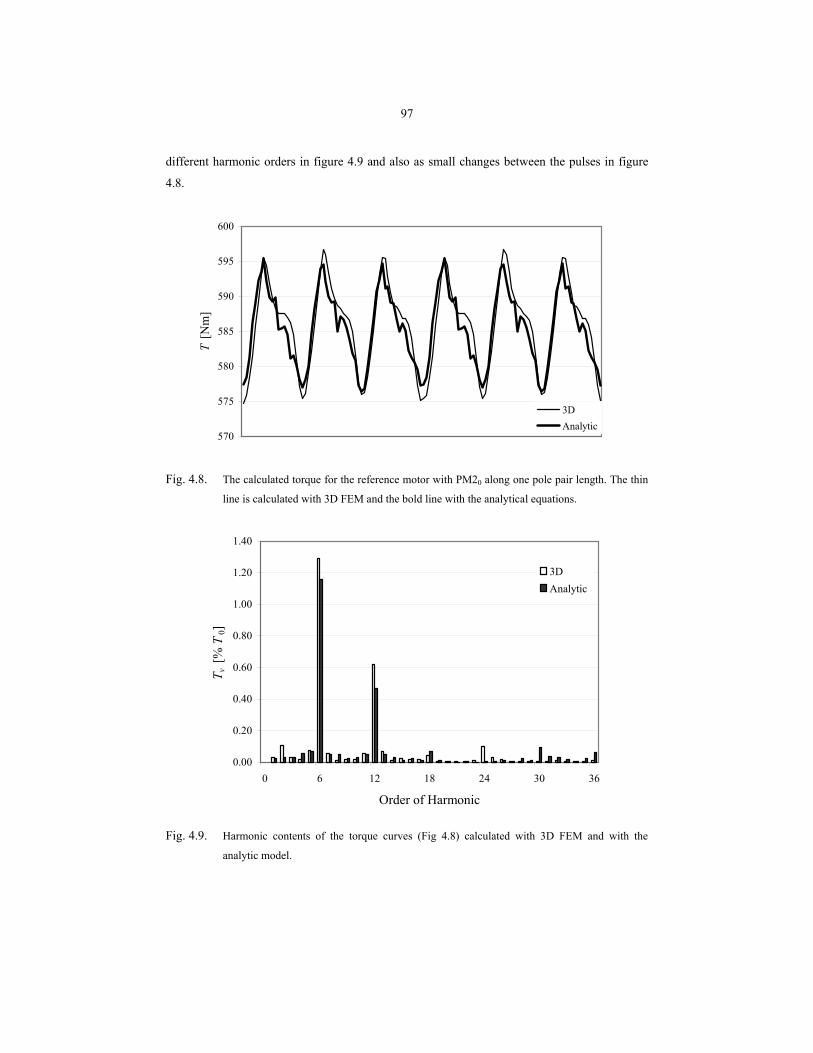
97
different harmonic orders in figure 4.9 and also as small changes between the pulses in figure
4.8.
570
575
580
585
590
595
600
T [N
m]
3DAnalytic
Fig. 4.8. The calculated torque for the reference motor with PM20 along one pole pair length. The thin
line is calculated with 3D FEM and the bold line with the analytical equations.
0.00
0.20
0.40
0.60
0.80
1.00
1.20
1.40
0 6 12 18 24 30 36
Order of Harmonic
T v [%
T0]
3DAnalytic
Fig. 4.9. Harmonic contents of the torque curves (Fig 4.8) calculated with 3D FEM and with the
analytic model.
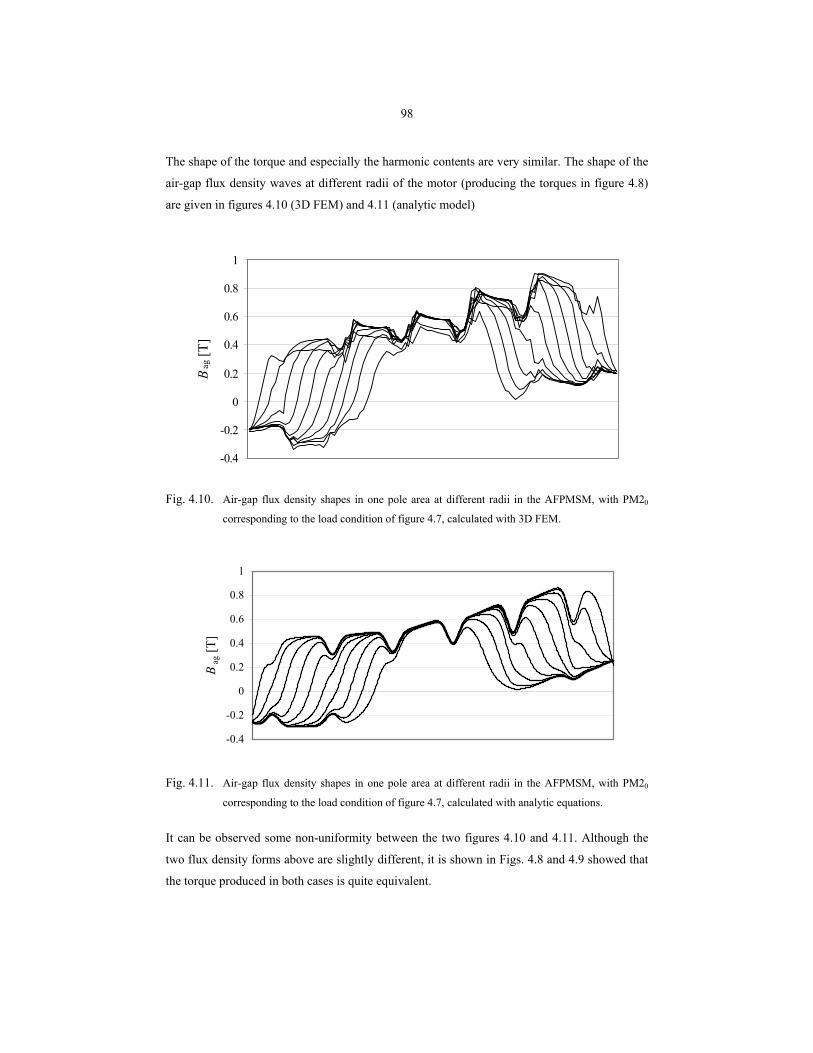
98
The shape of the torque and especially the harmonic contents are very similar. The shape of the
air-gap flux density waves at different radii of the motor (producing the torques in figure 4.8)
are given in figures 4.10 (3D FEM) and 4.11 (analytic model)
-0.4
-0.2
0
0.2
0.4
0.6
0.8
1
Bag
[T]
Fig. 4.10. Air-gap flux density shapes in one pole area at different radii in the AFPMSM, with PM20
corresponding to the load condition of figure 4.7, calculated with 3D FEM.
-0.4
-0.2
0
0.2
0.4
0.6
0.8
1
Bag
[T]
Fig. 4.11. Air-gap flux density shapes in one pole area at different radii in the AFPMSM, with PM20
corresponding to the load condition of figure 4.7, calculated with analytic equations.
It can be observed some non-uniformity between the two figures 4.10 and 4.11. Although the
two flux density forms above are slightly different, it is shown in Figs. 4.8 and 4.9 showed that
the torque produced in both cases is quite equivalent.
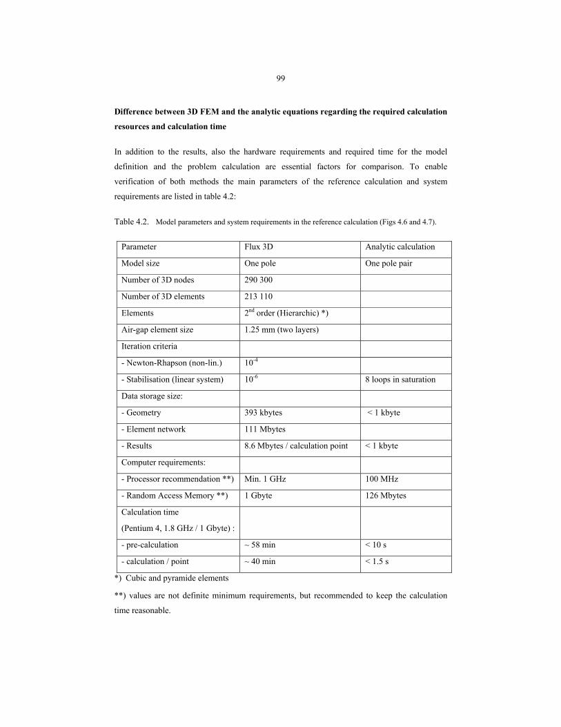
99
Difference between 3D FEM and the analytic equations regarding the required calculation
resources and calculation time
In addition to the results, also the hardware requirements and required time for the model
definition and the problem calculation are essential factors for comparison. To enable
verification of both methods the main parameters of the reference calculation and system
requirements are listed in table 4.2:
Table 4.2. Model parameters and system requirements in the reference calculation (Figs 4.6 and 4.7).
Parameter Flux 3D Analytic calculation
Model size One pole One pole pair
Number of 3D nodes 290 300
Number of 3D elements 213 110
Elements 2nd order (Hierarchic) *)
Air-gap element size 1.25 mm (two layers)
Iteration criteria
- Newton-Rhapson (non-lin.) 10-4
- Stabilisation (linear system) 10-6 8 loops in saturation
Data storage size:
- Geometry 393 kbytes < 1 kbyte
- Element network 111 Mbytes
- Results 8.6 Mbytes / calculation point < 1 kbyte
Computer requirements:
- Processor recommendation **) Min. 1 GHz 100 MHz
- Random Access Memory **) 1 Gbyte 126 Mbytes
Calculation time
(Pentium 4, 1.8 GHz / 1 Gbyte) :
- pre-calculation ~ 58 min < 10 s
- calculation / point ~ 40 min < 1.5 s
*) Cubic and pyramide elements
**) values are not definite minimum requirements, but recommended to keep the calculation
time reasonable.
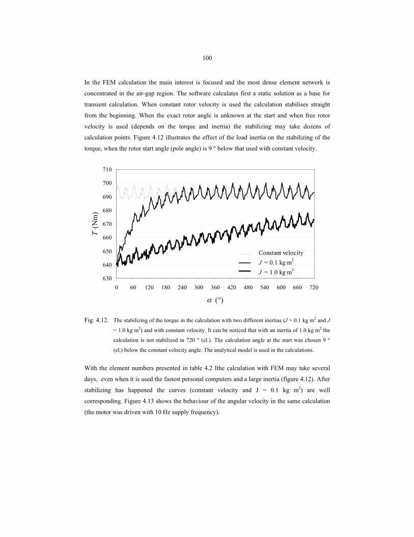
100
In the FEM calculation the main interest is focused and the most dense element network is
concentrated in the air-gap region. The software calculates first a static solution as a base for
transient calculation. When constant rotor velocity is used the calculation stabilises straight
from the beginning. When the exact rotor angle is unknown at the start and when free rotor
velocity is used (depends on the torque and inertia) the stabilizing may take dozens of
calculation points. Figure 4.12 illustrates the effect of the load inertia on the stabilizing of the
torque, when the rotor start angle (pole angle) is 9 ° below that used with constant velocity.
630
640
650
660
670
680
690
700
710
0 60 120 180 240 300 360 420 480 540 600 660 720
α (°)
T (N
m)
Constant velocityJ = 0.1 kg m2
J = 1.0 kg m2
Fig. 4.12. The stabilizing of the torque in the calculation with two different inertias (J = 0.1 kg m2 and J
= 1.0 kg m2) and with constant velocity. It can be noticed that with an inertia of 1.0 kg m2 the
calculation is not stabilized in 720 ° (el.). The calculation angle at the start was chosen 9 °
(el.) below the constant velocity angle. The analytical model is used in the calculations.
With the element numbers presented in table 4.2 Ithe calculation with FEM may take several
days, even when it is used the fastest personal computers and a large inertia (figure 4.12). After
stabilizing has happened the curves (constant velocity and J = 0.1 kg m2) are well
corresponding. Figure 4.13 shows the behaviour of the angular velocity in the same calculation
(the motor was driven with 10 Hz supply frequency).
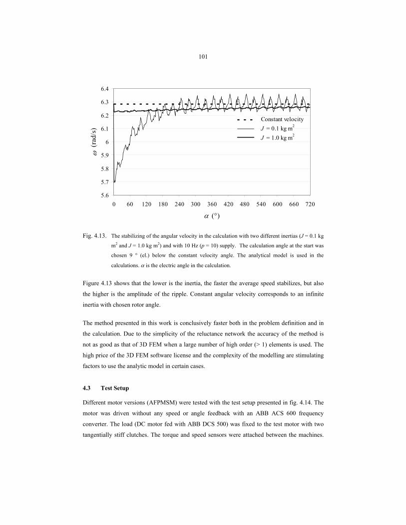
101
5.6
5.7
5.8
5.9
6
6.1
6.2
6.3
6.4
0 60 120 180 240 300 360 420 480 540 600 660 720
α (°)
ω (r
ad/s
)
Constant velocityJ = 0.1 kg m2
J = 1.0 kg m2
Fig. 4.13. The stabilizing of the angular velocity in the calculation with two different inertias (J = 0.1 kg
m2 and J = 1.0 kg m2) and with 10 Hz (p = 10) supply. The calculation angle at the start was
chosen 9 ° (el.) below the constant velocity angle. The analytical model is used in the
calculations. α is the electric angle in the calculation.
Figure 4.13 shows that the lower is the inertia, the faster the average speed stabilizes, but also
the higher is the amplitude of the ripple. Constant angular velocity corresponds to an infinite
inertia with chosen rotor angle.
The method presented in this work is conclusively faster both in the problem definition and in
the calculation. Due to the simplicity of the reluctance network the accuracy of the method is
not as good as that of 3D FEM when a large number of high order (> 1) elements is used. The
high price of the 3D FEM software license and the complexity of the modelling are stimulating
factors to use the analytic model in certain cases.
4.3 Test Setup
Different motor versions (AFPMSM) were tested with the test setup presented in fig. 4.14. The
motor was driven without any speed or angle feedback with an ABB ACS 600 frequency
converter. The load (DC motor fed with ABB DCS 500) was fixed to the test motor with two
tangentially stiff clutches. The torque and speed sensors were attached between the machines.
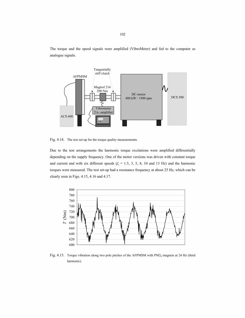
102
The torque and the speed signals were amplified (VibroMeter) and fed to the computer as
analogue signals.
AFPMSM
DC-motor 480 kW / 1500 rpm
Magtrol 214200 Nm
Tangentially stiff clutch
VibrometerT/n -amplifier
Labview
DCS 500
ACS 600
Fig. 4.14. The test set-up for the torque quality measurements.
Due to the test arrangements the harmonic torque excitations were amplified differentially
depending on the supply frequency. One of the motor versions was driven with constant torque
and current and with six different speeds (fs = 1.5, 3, 5, 8, 10 and 13 Hz) and the harmonic
torques were measured. The test set-up had a resonance frequency at about 25 Hz, which can be
clearly seen in Figs. 4.15, 4.16 and 4.17.
600620640660680700720740760780800
T (N
m)
Fig. 4.15. Torque vibration along two pole pitches of the AFPMSM with PM20 magnets at 24 Hz (third
harmonic).
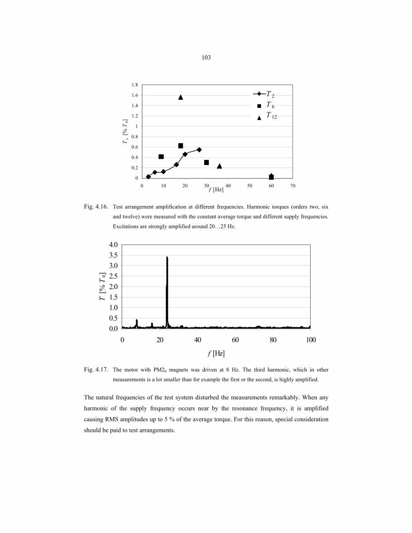
103
0
0.2
0.4
0.6
0.8
1
1.2
1.4
1.6
1.8
0 10 20 30 40 50 60 70f [Hz]
Tν
[% T
0]
T 2
T 6
T 12
Fig. 4.16. Test arrangement amplification at different frequencies. Harmonic torques (orders two, six
and twelve) were measured with the constant average torque and different supply frequencies.
Excitations are strongly amplified around 20…25 Hz.
0.00.51.01.52.02.53.03.54.0
0 20 40 60 80 100
f [Hz]
T [%
T0]
Fig. 4.17. The motor with PM20 magnets was driven at 8 Hz. The third harmonic, which in other
measurements is a lot smaller than for example the first or the second, is highly amplified.
The natural frequencies of the test system disturbed the measurements remarkably. When any
harmonic of the supply frequency occurs near by the resonance frequency, it is amplified
causing RMS amplitudes up to 5 % of the average torque. For this reason, special consideration
should be paid to test arrangements.
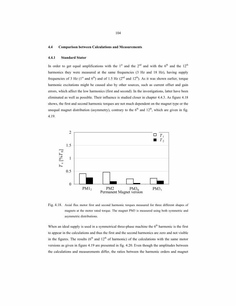
104
4.4 Comparison between Calculations and Measurements
4.4.1 Standard Stator
In order to get equal amplifications with the 1st and the 2nd and with the 6th and the 12th
harmonics they were measured at the same frequencies (3 Hz and 18 Hz), having supply
frequencies of 3 Hz (1st and 6th) and of 1.5 Hz (2nd and 12th). As it was shown earlier, torque
harmonic excitations might be caused also by other sources, such as current offset and gain
errors, which affect the low harmonics (first and second). In the investigations, latter have been
eliminated as well as possible. Their influence is studied closer in chapter 4.4.3. As figure 4.18
shows, the first and second harmonic torques are not much dependent on the magnet type or the
unequal magnet distribution (asymmetry), contrary to the 6th and 12th, which are given in fig.
4.19.
0
0.5
1
1.5
2
Permanent Magnet version
Tv [
%T
0]
T 1T 2
PM12 PM2 PM30 PM31
Fig. 4.18. Axial flux motor first and second harmonic torques measured for three different shapes of
magnets at the motor rated torque. The magnet PM3 is measured using both symmetric and
asymmetric distributions.
When an ideal supply is used in a symmetrical three-phase machine the 6th harmonic is the first
to appear in the calculations and thus the first and the second harmonics are zero and not visible
in the figures. The results (6th and 12th of harmonic) of the calculations with the same motor
versions as given in figure 4.19 are presented in fig. 4.20. Even though the amplitudes between
the calculations and measurements differ, the ratios between the harmonic orders and magnet
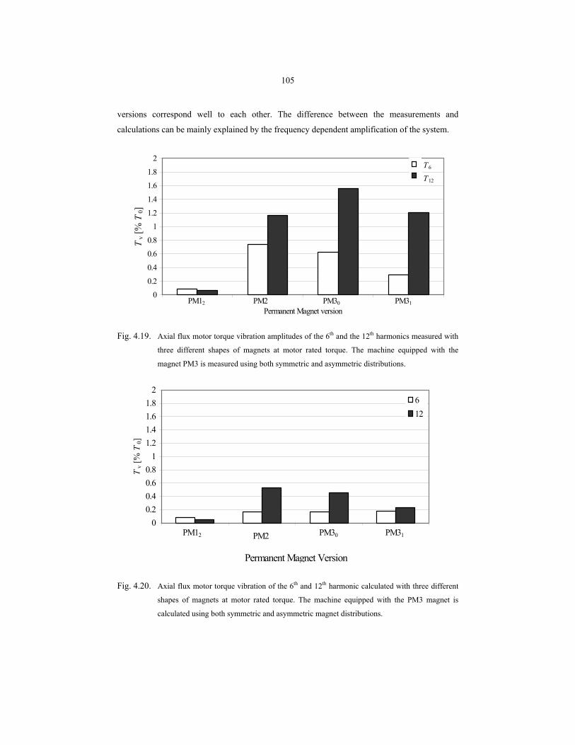
105
versions correspond well to each other. The difference between the measurements and
calculations can be mainly explained by the frequency dependent amplification of the system.
0
0.2
0.4
0.6
0.8
1
1.2
1.4
1.6
1.8
2
Permanent Magnet version
Tv [
% T
0]
T6
T12
PM12 PM2 PM30 PM31
Fig. 4.19. Axial flux motor torque vibration amplitudes of the 6th and the 12th harmonics measured with
three different shapes of magnets at motor rated torque. The machine equipped with the
magnet PM3 is measured using both symmetric and asymmetric distributions.
00.20.40.60.8
11.21.41.61.8
2
Permanent Magnet Version
Tv [
% T
0]
612
PM12 PM2 PM30 PM31
Fig. 4.20. Axial flux motor torque vibration of the 6th and 12th harmonic calculated with three different
shapes of magnets at motor rated torque. The machine equipped with the PM3 magnet is
calculated using both symmetric and asymmetric magnet distributions.
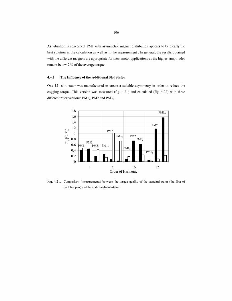
106
As vibration is concerned, PM1 with asymmetric magnet distribution appears to be clearly the
best solution in the calculation as well as in the measurement . In general, the results obtained
with the different magnets are appropriate for most motor applications as the highest amplitudes
remain below 2 % of the average torque.
4.4.2 The Influence of the Additional Slot Stator
One 121-slot stator was manufactured to create a suitable asymmetry in order to reduce the
cogging torque. This version was measured (fig. 4.21) and calculated (fig. 4.22) with three
different rotor versions: PM12, PM2 and PM30.
00.20.40.60.8
11.21.41.61.8
1 2 6 12Order of Harmonic
Tν [
% T
0]
PM12
PM2PM30
PM2
PM2
PM2
PM12 PM12PM12
PM30
PM30
PM30
Fig. 4.21. Comparison (measurements) between the torque quality of the standard stator (the first of
each bar pair) and the additional-slot-stator.
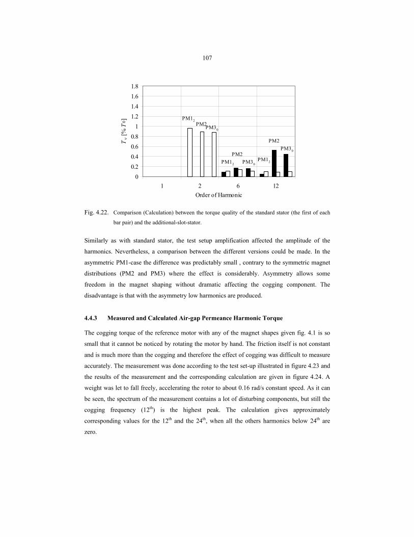
107
00.20.40.60.8
11.21.41.61.8
1 2 6 12Order of Harmonic
Tν [
% T
0 ] PM12PM2PM30
PM12PM12
PM2PM30
PM30
PM2
Fig. 4.22. Comparison (Calculation) between the torque quality of the standard stator (the first of each
bar pair) and the additional-slot-stator.
Similarly as with standard stator, the test setup amplification affected the amplitude of the
harmonics. Nevertheless, a comparison between the different versions could be made. In the
asymmetric PM1-case the difference was predictably small , contrary to the symmetric magnet
distributions (PM2 and PM3) where the effect is considerably. Asymmetry allows some
freedom in the magnet shaping without dramatic affecting the cogging component. The
disadvantage is that with the asymmetry low harmonics are produced.
4.4.3 Measured and Calculated Air-gap Permeance Harmonic Torque
The cogging torque of the reference motor with any of the magnet shapes given fig. 4.1 is so
small that it cannot be noticed by rotating the motor by hand. The friction itself is not constant
and is much more than the cogging and therefore the effect of cogging was difficult to measure
accurately. The measurement was done according to the test set-up illustrated in figure 4.23 and
the results of the measurement and the corresponding calculation are given in figure 4.24. A
weight was let to fall freely, accelerating the rotor to about 0.16 rad/s constant speed. As it can
be seen, the spectrum of the measurement contains a lot of disturbing components, but still the
cogging frequency (12th) is the highest peak. The calculation gives approximately
corresponding values for the 12th and the 24th, when all the others harmonics below 24th are
zero.
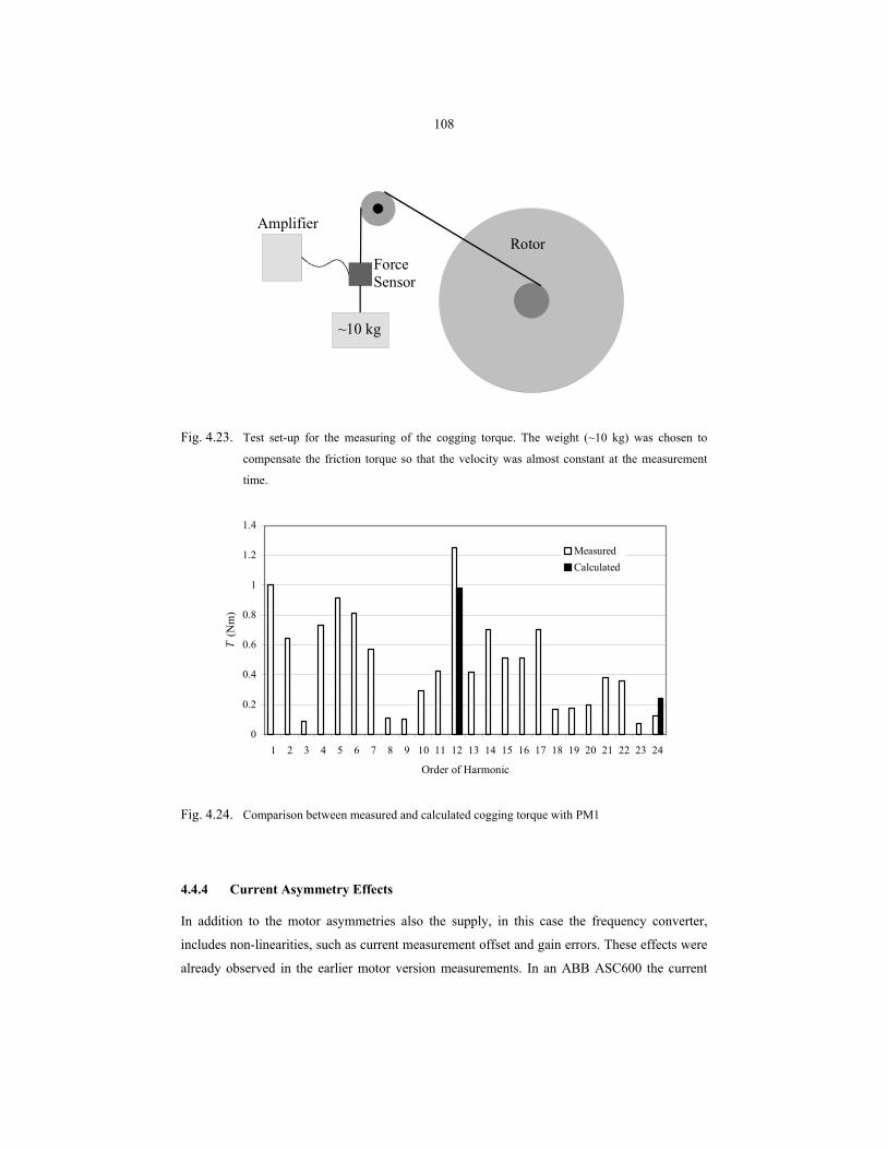
108
~10 kg
ForceSensor
RotorAmplifier
Fig. 4.23. Test set-up for the measuring of the cogging torque. The weight (~10 kg) was chosen to
compensate the friction torque so that the velocity was almost constant at the measurement
time.
0
0.2
0.4
0.6
0.8
1
1.2
1.4
1 2 3 4 5 6 7 8 9 10 11 12 13 14 15 16 17 18 19 20 21 22 23 24
Order of Harmonic
T (N
m)
MeasuredCalculated
Fig. 4.24. Comparison between measured and calculated cogging torque with PM1
4.4.4 Current Asymmetry Effects
In addition to the motor asymmetries also the supply, in this case the frequency converter,
includes non-linearities, such as current measurement offset and gain errors. These effects were
already observed in the earlier motor version measurements. In an ABB ASC600 the current
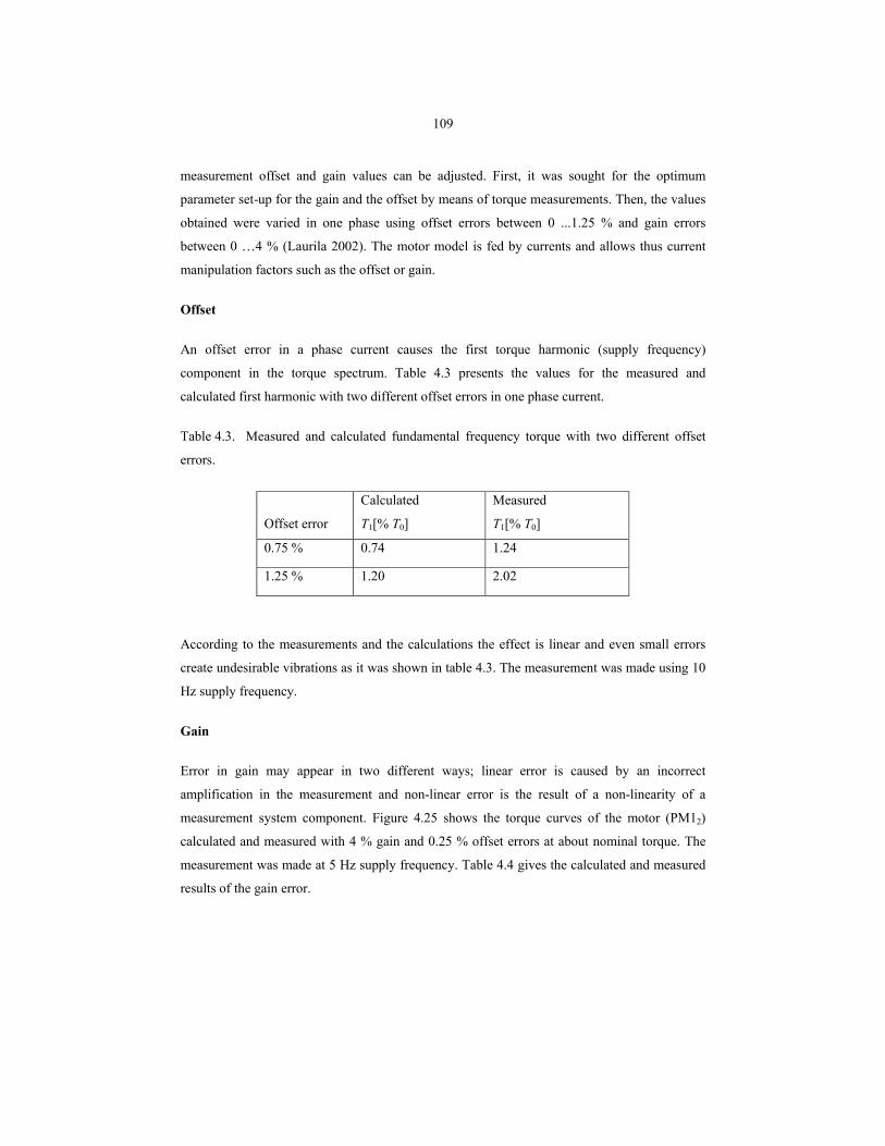
109
measurement offset and gain values can be adjusted. First, it was sought for the optimum
parameter set-up for the gain and the offset by means of torque measurements. Then, the values
obtained were varied in one phase using offset errors between 0 ...1.25 % and gain errors
between 0 …4 % (Laurila 2002). The motor model is fed by currents and allows thus current
manipulation factors such as the offset or gain.
Offset
An offset error in a phase current causes the first torque harmonic (supply frequency)
component in the torque spectrum. Table 4.3 presents the values for the measured and
calculated first harmonic with two different offset errors in one phase current.
Table 4.3. Measured and calculated fundamental frequency torque with two different offset
errors.
Offset error
Calculated
T1[% T0]
Measured
T1[% T0]
0.75 % 0.74 1.24
1.25 % 1.20 2.02
According to the measurements and the calculations the effect is linear and even small errors
create undesirable vibrations as it was shown in table 4.3. The measurement was made using 10
Hz supply frequency.
Gain
Error in gain may appear in two different ways; linear error is caused by an incorrect
amplification in the measurement and non-linear error is the result of a non-linearity of a
measurement system component. Figure 4.25 shows the torque curves of the motor (PM12)
calculated and measured with 4 % gain and 0.25 % offset errors at about nominal torque. The
measurement was made at 5 Hz supply frequency. Table 4.4 gives the calculated and measured
results of the gain error.
110
Table 4.4. Measured and calculated second harmonic torque with two different gain errors.
Gain error
Calculated
T2[% T0]
Measured
T2[% T0]
2.0 % 1.31 1.43
4.0 % 2.64 2.89
640
650
660
670
680
690
700
710
720
730
740
T (N
m)
Fig. 4.25. Motor torque (PM12) measured and calculated along two pole pitches with an one-phase gain
error of 4 % and with offset error 0.25%. The bold line is the calculated torque.
In the calculation only the linear component was considered. Table 4.4 and figure 4.25 show
that the calculation results match convincingly well the results obtained with the measurements.
4.5 Conclusions from the Comparison
The calculation procedure functions very reliably within the limits defined in the previous
chapters. Comparison with both FEM and the measurements shows that the results obtained
with the calculation procedure are promising.
It is shown that PM1 with asymmetric magnet distribution is obviously the most suitable
magnet shape. Unfortunately, the symmetric distribution variant of this magnet shape was not
available. Also the other magnet shapes (PM2 and PM3) are rather good and their use is
acceptable in most motor applications. With PM2 and PM3 the stator asymmetry reduces the
111
cogging in a considerable way and, for this reason, the results obtained are approaching those of
PM1. Due to the fact that the magnets in PM1 are already asymmetrically distributed, the
additional asymmetry in the stator does not have a big effect anymore.
The measuring arrangement with its natural frequencies made it difficult to get absolute
amplitudes of the harmonics, but the comparison between the magnets could be drawn
successfully.
The power supply (ABB ACS600) made it also possible to vary the source phase current
amplitude symmetry (gain and offset). The results obtained with the calculation and with the
measurements are satisfying.
112
5 Conclusions
In recent years it could be observed a considerable increase in the studying of permanent
magnet motor torque vibrations and especially of the cogging effect. Some of these studies
apply analytical methods, but most of them use FEM. The objective for this thesis was to
develop a simple but reliable calculation method for testing different factors of the motor and
improving the reference motor.
First target
The first goal of this study was to create an analytical calculation method for the purpose of
applying it to the surface mounted axial flux permanent magnet motor. The results have proven
that analytical equations can be used for PM-motor modelling. These do not compete with
FEM, but for certain purposes they may be applied and their application may also be considered
as a “pre study” to FEM use in order to reduce the required number of calculations or iterations.
As discussed in chapter four, the final result or absolute value is highly depended on the total
system and its frequency response and not just on the motor excitation. For this reason, the
effect generated by changes is often more interesting to study.
Analytical modelling offers several advantages:
- Easy modelling and parameter variation
- Easy to check the effect of different factors
- Fast calculation compared to FEM
- Can be modified for different accuracy levels (reluctance network)
- Equations easy to adapt for total (larger) systems
- Supply non-linearities can easily be considered
- Possible to use almost arbitrary magnet shape (constant thickness)
- Transients easy to calculate
The method has also some disadvantages and limitations compared to FEM. Of these it should
be mentioned:
- Equal magnet height is required
- Magnetic circuit details modelling is limited
113
- Magnetising direction is assumed to be constant
- Different type of motors require their own models
- Does not include all the options that are available in FEM => many features are
lacking
- Does not allow a same accuracy of fine modelling as FEM does
As a further disadvantage it should be noted that the different types of windings require their
own model/part. Consequently, this also means that the program can be applied to different
kinds of slotted windings by slightly manipulating it or by using separate models for the
different windings.
The structure of the reluctance network used appears to be rather simple, even so the calculation
results are promising when comparing them with the FEM results and with the measurements of
the actual models. This may be mainly explained by the fact that even a simple network is
capable of calculating reliably the instant flux in the teeth and thus the winding harmonics and
the average torque. The permeance harmonics are calculated using the permeance function, by
means of which the air-gap flux density can be accurately determined.
The Matlab-version of the calculation model has already been tested with the DTC –frequency
converter model and, in the near future, it will be joined to the electromechanical-system model.
Second target
The second purpose of the study was to apply the developed calculation program. By means of
the program the reference motor could be modified, the results achieved with FEM were
verified and measurements with actual models were carried out.
The significance of the magnet shape decreases if an additional slot stator is used. However, as
cogging is concerned, the results achieved are promising, and these results apply not only to
skewed magnets PM1 but also to all the other magnet types.
114
REFERENCES
Aydin, M., Huang, S., Lipo, T. A., (2001) Design and 3D Electromagnetic Field Analysis of Non-Slotted and Slotted TORUS Type Axial Flux Surface Mounted Permanent Magnet Disc Machines. The 27th Annual Conference of the IEEE Industrial Electronics Society. pp. 645-651.
Belachen A., (2000). Force Calculation for Vibration and Noise Analysis of Electrical Machines. International Conference of Electrical Motors 2000, Espoo Finland. pp. 1829-1833.
Bianchi, N., Cervaro, S., Malesani, L., (2000). Current Shapes for Minimising Torque Ripple in SPM Motors. International Conference of Electrical Motors 2000, Espoo Finland. pp. 1237-1241.
Bianchi, N.; Bolognani, S (2000). Design Techniques for Reducing the Cogging Torque in Surface-Mounted PM Motors. Industry Applications Conference, 2000. Conference Record of the 2000 IEEE, Vol. 1, 2000. pp. 179 –185
Boverket, (2002). Boverkets byggregler; Föreskrifter och almänna råd. Elanders Gotab, Vällingby.
Cai, W., Fulton, D., Reichrt, K., (2000). Design of Permanent Magnet Motors with Low Torque Ripples: A Review. International Conference of Electrical Motors 2000, Espoo Finland. pp. 1384-1388.
Chang, L., Dawson, G. E., Eastham, T. R., (1990). Permanent Magnet Synchronous Motor Design: Finite Element and Analytical Methods. International Conference of Electrical Motors 1990, Vol. III, pp. 1082-1088.
Chung, D-W., Sul, S-K., (1998). Analysis and Compensation of Current Measurement Error in Vector-Controlled AC Motor Drives. IEEE Transactions on Industrial Applications, Volume: 34, No: 2, pp. 340 – 345.
Chung, M-J., Gweon, D-G., (2001). Modelling of the Armature Slotting Effect of Magnetic Field Distribution of a Linear Permanent Magnet Motor. Electrical Engineering 84, 2002. pp. 101-108.
Colamartino, F.; Marchand, C.; Razek, A., (1994). Considerations of Non-Sinusoidal Field Distribution in a Permanent Magnet Synchronous Motor Control. Fifth International Conference on Power Electronics and Variable-Speed Drives 1994 , pp. 508 –513
Consoli, A., Oteri, F., Raciti, A., (1990). Dynamic Behaviour of Permanent Magnet Synchronous Machines. International Conference of Electrical Motors 1990, Vol. I, pp. 117-123.
De La Ree, J., Boules, N., (1989). Torque production in Permanent Magnet Synchronous Motors. IEEE Transactions on Industry Applications Vol 25, NO. 1. 1989. pp. 107-111.
Gieras, J. F., Piech, Z. J., (1999), Linear Synchronous Motors: Transportation and Automation Systems, CRC Press, London, New York, Washington DC.
Hakala, H., (1995). Applications of Linear Motors in Elevator Hoisting Machines. Dissertation, Tampere University of technology.
115
Hanselman, D. C., (1994) Brushless Permanent Magnet Motor Design. McGraw-Hill, New York, p.22.
Heikkilä, T., (2002). Permanent Magnet Synchronous Motor for Industrial Applications – Analysis and Design. Dissertation, Lappeenranta University of Technology.
Heller, B., Hamata, V., (1977). Harmonic Field Effects in Induction Machines, Elsevier Scientific Publishing Company, Amsterdam, Oxford, New York.
Hendershot Jr, J.R., Miller, T. J. E., (1994). Design of Brushless Permanent-Magnet Motors, Magna Physics Publishing and Clarendon Press, Oxford.
Hirvonen, M., (1997) Epäsinimuotoisen ilmavälivuon kestomagneettitahtikoneen suoralle vääntömomentin säädölle asettamat erityisvaatimukset. Thesis for Master of Science, Lappeenranta University of Technology (in Finnish).
Huang, S., Aydin, M, Lipo, T. A., (2001). Electromagnetic Vibration and Noise Assessment for Surface Mounted PM Machines. The 27th Annual Conference of the IEEE Industrial Electronics Society. pp 1417-1426.
Ishikawa, T.; Slemon, G.R. (1993). A Method of Reducing Ripple Torque in Permanent Magnet Motors Without Skewing., IEEE Transactions on Magnetics, Volume: 29 Issue: 2 , March 1993. pp. 2028 –2031.
Jahns, T.M.; Soong, W.L., (1996). Pulsating Torque Minimization Techniques for Permanent Magnet AC Motor Drives-a Review., IEEE Transactions on Industrial Electronics, Volume: 43 Issue: 2 , April 1996. pp. 321 –330
Kaukonen, J., (1994). Energy Consumption Losses of Induction motors in Pulp and Paper Industry. Thesis for Master of Science, Lappeenranta University of Technology (in Finnish).
Kaukonen, J., Pyrhönen, J., Nerg, J., Luukko, J., Niemelä, M., Pyrhönen, O., (1998). Salient Pole Synchronous Motor Saturation in a Direct Torque Controlled Drive International Conference of Electrical Motors 1998. pp. 1397-1401.
Kim, U., Lieu, D.K., (1998). Magnetic Field Calculation in Permanent Magnet Motors with Rotor Eccentricity: Without Slotting Effect. IEEE Transactions on Magnetics, Volume: 34 Issue: 4 Part: 2, pp. 2243 –2252
Laurila, L., Kurronen, P., Niemelä, M., Pyrhönen, J., (2002). Effect of Unideal Current Sensors in Direct Torque Controlled PMSM Drives. NORPIE 2002, Nordic Workshop on Power and Industrial Electronics.
Li, T., Slemon, G. (1988). Reduction of Cogging Torque in Permanent Magnet Motors. IEEE Transactions on Magnetics, Volume: 24 Issue: 6, Nov. 1988. pp. 2901 –2903
Lukaniszyn, M., Wrobel, R., (2000). A Study on the Influence of Permanent Magnet Dimensions and Stator Core Structures on the Torque of the Disc-Type Brushless DC Motor. Electrical Engineering 82, 2000. pp. 163-171.
116
Luukko, J., (2000). Direct Torque Control Of Permanent Magnet Synchronous Machines – Analysis and Implementation. Dissertation, Lappeenranta University of Technology.
Neorem Magnets Oy (2003). Technical pages in www.neorem.fi (Internet 28.02.2003)
Newland, D. E.,(1989). Mechanical Vibration Analysis and Computation. Longman Scientific and Technical
Nipp, E., Reduction of Torque Ripple and Current Harmonics in Surface-Mounted Permanent Magnet Motors. International Conference of Electrical Motors 1996, Vol. II, pp. 273-278.
Pahner, U., Van Haute, S., Belmans, R., Hameyer, K., Stumberger, B., Dolinar, D., (1998). Comparison of Two Methods to Determine the d/q-axis Lumped Parameters of Permanent Magnet Machines with Respect to Numerical Optimisation. International Conference of Electrical Motors 1998. pp. 352-357.
Paljan, D., (2000). Magnetischer Leitwert des Exzentrischen Luftspaltes bei Electrischen Maschinen. Electrical Engineering 82 (2000), pp. 247-255.
Parviainen, A., Pyrhönen, J., Niemelä, M., 2001, Axial Flux Interior Permanent Magnet Synchronous Motor with Sinusoidally Shaped Magnets, ISEF 2001 - 10th International Symposium on Electromagnetic Fields in Electrical Engineering Cracow, Poland, September 20-22, 2001
Perho, J., (2002). Reluctance Network for Analysing Induction Machines. Dissertation, Helsinki University of Technology.
Proca, A.B.; Keyhani, A.; EL-Antably, A. (1999). Analytical model for permanent magnet motors with surface mounted magnets. Electric Machines and Drives, 1999. International Conference IEMD '99. , Page(s):767 – 769.
Pyökäri, T., (1971). Sähkökoneoppi (Electric Motor Theory), Weilin + Göös (in Finnish).
Pyrhönen, J. (1991). Magneettiset materiaalit (Magnetic Materials), Lappeenranta University of Technology, Research report EN B-74 (in finnish).
Pyrhönen, J. (2003). Sähkökoneopas. Lappeenranta University of Technology. Education Material (in Finnish)
Pyrhönen, J., Kurronen, P., (1993). Properties of High-Speed Solid-Rotor Induction Machines. Lappeenranta University of Technology. Research report EN A-19.
Rasmussen, K. F., (1999). Analytical Prediction of Magnetic Field from Surface Mounted Permanent Magnet Motor. Electric Machines and Drives, 1999. International Conference IEMD '99. , Page(s):34 – 36
Roisse, H., Brochet, P., (1996). Dynamic Simulation of a Synchronous Permanent Magnet Machine Using a Coupled Permeance Network. International Conference of Electrical Motors 1996, Vol II, pp. 39-44.
Romary, R., Roger, D., Brudny, J.F., Brutsaert, P., (1994). Rejection of Tangential Vibrations of Synchronous Machine Under Speed Control. Fifth International Conference on Power Electronics and Variable-Speed Drives, 1994. pp. 574 –579.
117
Sahin, F., Vandenput, A. J. A., Thermal Modeling and Testing of a High-Speed Axial Flux Permanent-Magnet Machine. ICEM 2002
Sebastian, T., Gangla, V., (1996). Analysis of Induced EMF Waveforms and Torque Ripple in a Brushless Permanent Magnet Machine. IEEE Transactions on Industry Applications Vol. 32, NO. 1, 1996. pp. 195-200.
Sitapati, K., Krishnan, R., (2001). Performance Comparisons of Radial and Axil Field, Permanent Magnet, Brushless Machines. IEEE Transactions on Industry Applications Vol 37, NO. 5, 2001. pp. 1219-1226.
Studer, C.; Keyhani, A.; Sebastian, T.; Murthy, S.K, (1997). Study of Cogging Torque in Permanent Magnet Machines. Industry Applications Conference, 1997. Thirty-Second IAS Annual Meeting, IAS '97. Conference Record of the 1997 IEEE Vol. I, 1997 , pp. 42 -49
Stumberger, B., Kreca, B., Hribernik, B., (1996). Variation of Parameters of Two Axis Model of Synchronous Motor with Permanent Magnets. International Conference of Electrical Motors 1996, Vol I, pp. 12-16.
Wang, J-P., Leiu, D. K., (1999). Magnetic Lumped Parameter Modelling of Rotor Eccentricity in Brushless Permanent-Magnet Motors. IEEE Transactions on Magnetics, Volume: 35 Issue: 5. pp. 4225 –4231.
Weber, W., (1928). Nutungsfactor in Electrischen Maschinen. ETZ 1928, pp. 858 – 861.
Zhang, Z., Profumo, F., Tenconi., (1996). Axial Flux Versus Radial Flux PM Motors. Speedam ‘96, Capri, Italy. pp. A4 – 19 -24.
Zhu, Z. Q. Howe, D., Bolte, E., Ackerman, B., (1993) Instantaneous Magnetic Field Distribution in Brushless Permanent Magnet dc Motors, Part I: Open-Circuit Field. IEEE Transactions on Magnetics Vol 29, NO. 1.
Zhu, Z.Q.; Howe, D. Influence of Design Parameters on Cogging Torque in Permanent Magnet Machines., IEEE Transactions on Energy Conversion, Volume: 15 Issue: 4 , Dec. 2000. pp. 407 -412
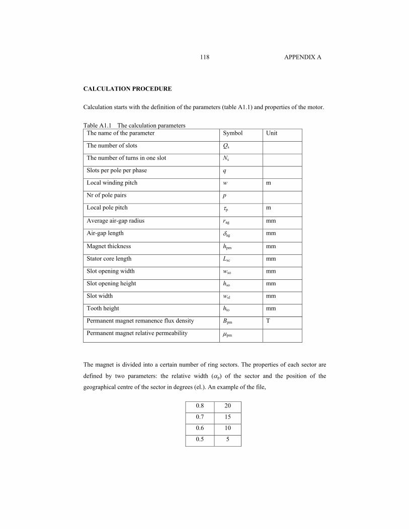
APPENDIX A 118
CALCULATION PROCEDURE
Calculation starts with the definition of the parameters (table A1.1) and properties of the motor.
Table A1.1 The calculation parameters The name of the parameter Symbol Unit
The number of slots Qs
The number of turns in one slot Ns
Slots per pole per phase q
Local winding pitch w m
Nr of pole pairs p
Local pole pitch τp m
Average air-gap radius rag mm
Air-gap length δag mm
Magnet thickness hpm mm
Stator core length Lsc mm
Slot opening width wso mm
Slot opening height hso mm
Slot width wsl mm
Tooth height hto mm
Permanent magnet remanence flux density Bpm T
Permanent magnet relative permeability µpm
The magnet is divided into a certain number of ring sectors. The properties of each sector are
defined by two parameters: the relative width (αp) of the sector and the position of the
geographical centre of the sector in degrees (el.). An example of the file,
0.8 20
0.7 15
0.6 10
0.5 5
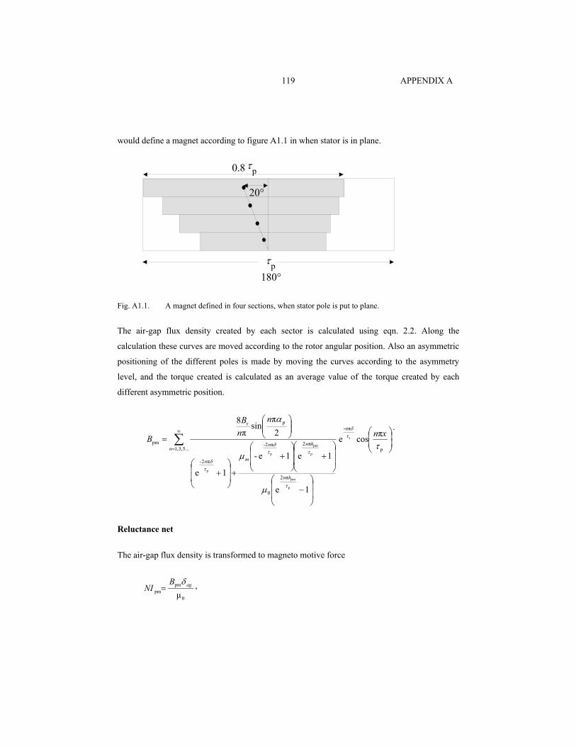
APPENDIX A 119
would define a magnet according to figure A1.1 in when stator is in plane.
τp180°
0.8 τp
20°
Fig. A1.1. A magnet defined in four sections, when stator pole is put to plane.
The air-gap flux density created by each sector is calculated using eqn. 2.2. Along the
calculation these curves are moved according to the rotor angular position. Also an asymmetric
positioning of the different poles is made by moving the curves according to the asymmetry
level, and the torque created is calculated as an average value of the torque created by each
different asymmetric position.
−
+
+
+
+
= ∑∞
= p
π-
...5,3,1
π2
0
π2π2-
π2-
pr
pmπcose
1e
1e1e-
1e
2π
sinπ
8
s
p
pm
p
pm
p
p
τ
µ
µ
α
τδ
τ
ττδ
τδ
xnn
nB
Bn
n
hn
hnn
mn
.
Reluctance net
The air-gap flux density is transformed to magneto motive force
0
pmpm µ
agBNI
δ= ,
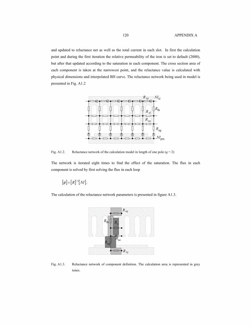
APPENDIX A 120
and updated to reluctance net as well as the total current in each slot. In first the calculation
point and during the first iteration the relative permeability of the iron is set to default (2000),
but after that updated according to the saturation in each component. The cross section area of
each component is taken at the narrowest point, and the reluctance value is calculated with
physical dimensions and interpolated BH curve. The reluctance network being used in model is
presented in Fig. A1.2
NIpm
NIsl
Rag
RthR sl
Rso
R sy
Fig. A1.2. Reluctance network of the calculation model in length of one pole (q = 2)
The network is iterated eight times to find the effect of the saturation. The flux in each
component is solved by first solving the flux in each loop
[ ] [ ] [ ]NIR 1−=φ .
The calculation of the reluctance network parameters is presented in figure A1.3.
R sy
Rth
R ry
Rso
Rs
Rag
Fig. A1.3. Reluctance network of component definition. The calculation area is represented in grey
tones.
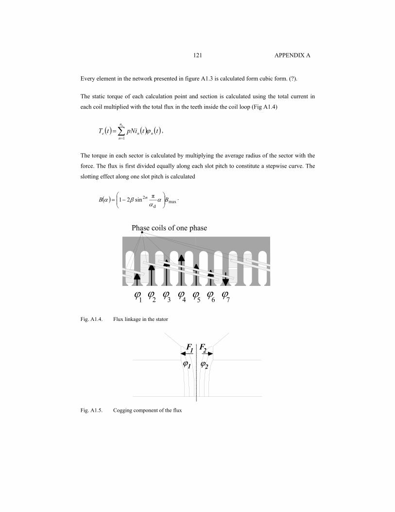
APPENDIX A 121
Every element in the network presented in figure A1.3 is calculated form cubic form. (?).
The static torque of each calculation point and section is calculated using the total current in
each coil multiplied with the total flux in the teeth inside the coil loop (Fig A1.4)
( ) ( ) ( )∑=
=c
1
n
nnne ttpNitT ϕ ,
The torque in each sector is calculated by multiplying the average radius of the sector with the
force. The flux is first divided equally along each slot pitch to constitute a stepwise curve. The
slotting effect along one slot pitch is calculated
( ) maxd
2 πsin21 BB n
−= α
αβα .
ϕ1
ϕ2
ϕ3
ϕ4
ϕ5
ϕ6
ϕ7
Phase coils of one phase
Fig. A1.4. Flux linkage in the stator
ϕ1 ϕ2
F1 F2
Fig. A1.5. Cogging component of the flux
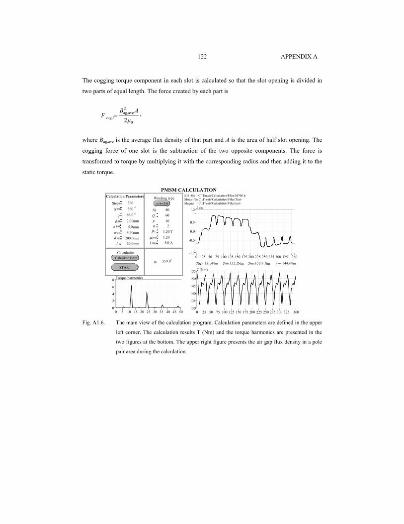
APPENDIX A 122
The cogging torque component in each slot is calculated so that the slot opening is divided in
two parts of equal length. The force created by each part is
0
2ag,ave
cog, 2µAB
F i= ,
where Bag,ave is the average flux density of that part and A is the area of half slot opening. The
cogging force of one slot is the subtraction of the two opposite components. The force is
transformed to torque by multiplying it with the corresponding radius and then adding it to the
static torque.
359.0α 151.4T(α)
1.2
-1.2
-0.5
0.0
0.5
360 0 25 50 75 100 125 150 175 200 225 250 275 300 325
B gap
1.20B r 1.20µ pm
10p
200.0 R ag 4.50 w so
60Q 66.0 γ
5.0I rms
Calculate Bpm Calculation
155
130
135
140
145
150
360 0 25 50 75 100 125 150 175 200 225 250 275 300 325
T (Nm)
360 Steps 360 α max
C:\Thesis\Calculation\Files\M700.bBH -fileC:\Thesis\Calculation\Files\Test-Motor file
60.0 L sc
80N s
8
0 2 4 6
500 5 10 15 20 25 30 35 40 45
Torque harmonics
144.4 Tave
2.00 δ m 5.0 h PM
mm
mm mm
A
Nm
mm
mm
T
°
°
Calculation Parameters
Nm
PMSM CALCULATION
°
START 132.2Tmin 153.7Tmax
2q
w/t=5/6Winding type
C:\Thesis\Calculation\Files\test-Magnet
Nm Nm
Fig. A1.6. The main view of the calculation program. Calculation parameters are defined in the upper
left corner. The calculation results T (Nm) and the torque harmonics are presented in the
two figures at the bottom. The upper right figure presents the air gap flux density in a pole
pair area during the calculation.
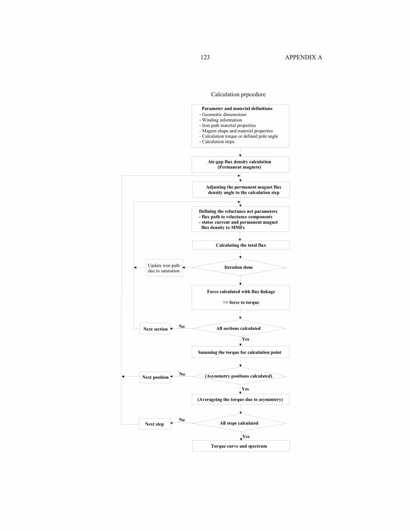
APPENDIX A 123
Parameter and material definitions- Geometric dimenssions- Winding information- Iron path material properties- Magnet shape and material properties- Calculation torque or defined pole angle- Calculation steps
Air-gap flux density calculation(Permanent magnets)
Adjusting the permanent magnet flux density angle to the calculation step
Calculating the total flux
Defining the reluctance net parameters- flux path to reluctance components- stator current and permanent magnet flux density to MMFs
Iteration doneUpdate iron path due to saturation
Force calculated with flux linkage
=> force to torque
Summing the torque for calculation point
All sections calculated
(Averageing the torque due to asymmtery)
(Asymmetry positions calculated)
Torque curve and spectrum
All steps calculatedNext step
Next position
No
No
Yes
Yes
Yes
Next section No
Calculation prpcedure
ACTA UNIVERSITATIS LAPPEENRANTAENSIS
111. LAINE, PERTTI. Kohti vesiensuojelun aikaa: veden laadun muutokset eteläisellä Saimaalla. 2001. 264 s. Väitösk.
112. SILVENTOINEN, PERTTI. Electromagnetic compatibility and EMC-measurements in DC-voltage link converters. 2001. 115 s. Diss.
113. TERVONEN, ANTERO. Laadun kehittäminen suomalaisissa yrityksissä. 2001. 206 s. Väitösk.
114. SALMINEN, ANTTI. The effects of filler wire feed on the efficiency, parameters and tolerances of laser welding. 2001. 82 s., liitt. Diss.
115. HORTTANAINEN, MIKA. Propagation of the ignition front against airflow in packed beds of wood particles. 2001. U.s. Diss.
116. IKONEN, JOUNI. Improving distributed simulation in a workstation environment. 2001. U.s. Diss.
117. WU, HUAPENG. Analysis, design and control of a hydraulically driven parallel robot manipulator. 2001. U.s. Diss.
118. REUNANEN, ARTTU. Experimental and numerical analysis of different volutes in a centrifugal compressor. 2001. 150 s. Diss.
119. TAAVITSAINEN, VELI-MATTI. Strategies for combining soft and hard modelling in some physicochemical problems. 2001. U.s. Diss.
120. SAVOLAINEN, RAIJA. The use of branched ketene dimers in solving the deposit problems related to the internal sizing of uncoated fine paper. 2001. U.s. Diss.
121. SARAVIRTA, ALI. Project success through effective decisions: case studies on project goal setting, success evaluation and managerial decision making. 2001. 286 s. Diss.
122. BLOMQVIST, KIRSIMARJA. Partnering in the dynamic environment: the role of trust in asymmetric technology partnership formation. 2002. 296 s., liitt. Diss.
123. KARVONEN, VESA. Development of fiber recovery process. 2002. U.s. Diss.
124. KÄYHKÖ, JARI. The influence of process conditions on the deresination efficiency in mechanical pulp washing. 2002. 87 s., liitt. Diss.
125. SAVOLAINEN, PEKKA. Modeling of non-isothermal vapor membrane separation with thermodynamic models and generalized mass transfer equations. 2002. 179 s. Diss.
126. KÄRKKÄINEN, HANNU. Customer need assessment: Challenges and tools for product innovation in business-to-business organizations. 2002. U. s. Diss.
127. HÄMÄLÄINEN, MARKKU. Spray coating technique as a surface treatment for woodcontaining paper grades. 2002. 121 s. Diss.
128. RANTA, TAPIO. Logging residues from regeneration fellings for biofuel production – a GIS-based availability and supply cost analysis. 2002. 182 s. Diss.
129. KUOSA, MAUNU. Numerical and experimental modelling of gas flow and heat transferin the air gap of an electric machine. 2002. 97 s. Diss.
130. LAITINEN, NIINA. Development of a ceramic membrane filtration equipment and its applicability for different wastewaters. 2002. U. s. Diss.
131. SUNDQVIST, SANNA. Market orientation in the international context: Antecedents, consequences and applicability. 2002. U. s. Diss.
132. TORKKELI, MARKO. Technology selection and group decision support systems: Case studies on supporting strategic technology selection processes. 2002. U.s. Diss.
133. KYRKI, VILLE. Local and global feature extraction for invariant object recognition. 2002. 115 s. Diss.
134. HEIKKILÄ, TANJA. Permanent magnet synchronous motor for industrial inverter applications – analysis and design. 2002. 109 s. Diss.
135. HUTTUNEN, PENTTI. Data-parallel computation in parallel and distributed environments. 2002. U.s. Diss.
136. LIU, YONG. On sliding mode control of hydraulic servo systems and a manipulator. 2002. U.s.Diss.
137. JUHANTILA, OLLI-PEKKA. Establishing intercompany relationships: Motives and methods for successful collaborative engagement. 2002. 281 s. Diss.
138. PREIS, SERGEI. Practical applications of a systematic approach to the chemical abatement of pollutants in water and air. 2002. 234 s. Diss.
139. TIIHONEN, JARI. Influence of stationary phase and eluent properties on chromatographic separation of carbohydrates. 2002. U. s. Diss.
140. KILKKI, JUHA. Automated formulation of optimisation models for steel beam structures. 2002. 85 s., liitt. Diss.
141. LENSU, LASSE. Photoelectric properties of bacteriorhodopsin films for photosensing and information processing. 2002. 114 s. Diss.
142. KAURANNE, TUOMO. Introducing parallel computers into operational weather forecasting. 2002. U.s. Diss.
143. PUUMALAINEN, KAISU. Global diffusion of innovations in telecommunications: Effects of data aggregation and market environment. 2002. 153 s. Diss.
144. SARRETTE, CHRISTINE. Effect of noncondensable gases on circulation of primary coolant in nuclear power plants in abnormal situations. 2003. 114 s. Diss.
145. SAARENKETO, SAMI. Born globals – internationalization of small and medium-sized knowledge-intensive firms. 2002. 247 s. Diss.
146. IKONEN, KIRSI. Metal surface and subsurface inspection using nondestructive optical methods. 2002 U.s. Diss.
147. KOUVO, PETRI. Formation and control of trace metal emissions in co-firing of biomass, peat and wastes in fluidised bed combustors. 2003. U.s. Diss.
148. MOOSAVI, ALI. Transport properties of multi-phase composite materials. 2003. U.s. Diss.
150. SMOLANDER, KARI. On the role of architecture in systems development. 2003. U.s. Diss.
151. VERENICH, SVETLANA. Wet oxidation of concentrated wastewaters: process combination and reaction kinetic modeling. 2003. U.s. Diss.
152. STÅHLE, PIRJO, STÅHLE, STEN & PÖYHÖNEN, AINO. Analyzing dynamic intellectual capital: System-based theory and application. 2003. 191 s.
153. HAATAJA, JORMA. A comparative performance study of four-pole induction motors and synchronous reluctance motors in variable speed drives. 2003. 135 s. Diss.
Recommended