The macroeconomic effects of the sovereign debt crisis in the euro area
Stefano Neri and Tiziano Ropele*
May 2013
Abstract
Since the spring of 2010 tensions in the government bond markets in the euro-area have led to diverging dynamics in the cost of loans and credit developments among euro-area countries. These heterogeneous credit conditions, together with fiscal consolidations in some countries, have led to diverging trends in economic activity and employment. This paper studies the macroeconomic effects of the sovereign debt crisis focusing on a subset of euro-area countries using a Factor Augmented Vector Autoregressive (FAVAR) model. The analysis suggests that the sovereign tensions have led to an increase in the cost of new loans and a contraction in credit which has been particularly strong in the countries most affected by the crisis. The higher cost of credit and the contraction in lending have exerted a negative and significant effect on industrial production in both the peripheral and core countries. In the latter countries, the contraction in economic activity has reflected the strong trade link with the peripheral countries. The findings are robust to an alternative transformation of the data and measure of sovereign tensions.
JEL codes: E52, F41.
Keyword: sovereign debt crisis; FAVAR; Bayesian methods.
Paper presented at the Workshop “The Sovereign Debt Crisis and the Euro Area” organized by the Bank of Italy and held in Rome on February 15, 2013. The proceedings are available at:http://www.bancaditalia.it/studiricerche/convegni/atti.
* Bank of Italy, Economic Research and International Relations Area, Economic Outlook and Monetary Policy Department. We thank Fabio Canova, Francesco Nucci, Marco Lippi, Giulio Nicoletti, Marco Lombardi, Frank Smets, Giancarlo Corsetti and Gabriel Perez-Quiros for their comments and suggestions. The views expressed in the paper do not necessarily reflect those of the Banca d’Italia. All errors are the responsibility of the authors.
268
1. Introduction
The sovereign debt crisis that erupted in early 2010 has led to dramatic economic and social
consequences. The widening of sovereign spreads in several euro-area countries has been
accompanied by divergent financial and macroeconomics developments. While in the “core”
countries (Germany, Netherlands, France, Austria, Belgium and Finland) financing conditions
remained broadly in line with the European Central Bank (ECB) official rates, industrial production
continued expanding and unemployment barely increased, in the “peripheral” countries (Greece,
Ireland, Portugal, Spain and Italy) the picture was literally reversed. Credit became more costly and
scantier, economic activity fell and unemployment increased. At the apex of the financial tensions
in the last quarter of 2011, the survival of the euro area was at risk. The ECB and the national
governments intervened with bold measures to restore confidence in financial markets, to support
the flow of credit to the economy and to guarantee the sustainability of public finances.
In this paper we propose a quantification of the impact of the sovereign debt crisis on a
number of macroeconomic variables, pertaining not only to the euro area as a whole but also to
individual countries. Our interest in documenting the effects of the sovereign tensions on country-
specific variables not only arises naturally because the debt crisis has exerted heterogeneous effects
on member countries but also because shedding light on its transmission mechanisms may help
shaping policy-makers’ interventions.
The outburst of the sovereign debt crisis in the euro area has attracted a lot of attention from
central banks, international institutions, and academic researchers. However, to the best of our
knowledge no paper has yet attempted a quantification of the macroeconomic impact of the
sovereign crisis. In order to fill this gap, three important issues need to be resolved beforehand.
First, how can one identify a “sovereign tensions” shock? Second, how can one deal with a
potentially very large set of macroeconomic variables? Third, given that the tensions started at the
end of 2009, how can one study the effects of the crisis using a limited sample size?
269
With regard to the first issue, given the uniqueness of the euro-area sovereign debt crisis,
there is not a commonly and widely accepted indicator of sovereign tension. For this reason we
propose three possible indicators, all of which are based on sovereign bonds yields. The first
indicator builds on the so-called “wake-up call” hypothesis and consists of the spread between the
10-year Greek bonds yield and the interest rate swap of corresponding maturity. The second one
exploits the results of a principal component analysis (PCA) on the whole set of sovereign spreads
and is constructed as a weighted average of the spreads between the 10-year Italian, Greek, Irish,
Portuguese, Spanish, Belgian, French and Austrian bonds yield and the interest rate swap of
corresponding maturity. The last indicator consists of the first principal component of the whole set
of sovereign spreads.
With regards to the second issue on how to handle a high-dimension data set, we conduct our
empirical investigation estimating a Factor Augmented Vector Autoregressive (FAVAR) model
with Bayesian methods. The FAVAR methodology, popularized by Bernanke, Boivin and Eliasz
(2005), has been shown to be a suitable tool to examine the effects of shocks on high-dimension
dataset. Our analysis employs a total of 139 time series regarding industrial production, bank
interest rates, credit and monetary aggregates, inflation and unemployment rates at the national
level and a set of aggregate variables for the euro area.
Finally, on the third issue we base our analysis solely on monthly time series observed from
January 2008 to September 2012 and we use Bayesian methods.1 In particular, Bayesian estimation
allowed us to estimate the VAR over a short sample by employing prior distributions for the
parameters of the model.
Our results can be summarised as follows. An adverse “sovereign tensions” shock, besides
increasing sovereign spreads in the peripheral countries, leads to significantly heterogeneous credit
conditions and credit dynamics across euro-area member countries. However, the impact on
industrial activity is rather similar across countries, possibly reflecting the strong trade links 1 As explained more in detail in Section 4.1, the estimation of the factors has been done using the sample period from January 2003 to September 2012.

270
between peripheral and “core” countries. The diverging trends in unemployment may be related to
structural differences, including job protection and labour market flexibility. These findings are
robust to a different transformation of the data and to alternative indicators of sovereign debt
tensions.
2. The macroeconomic effects of sovereign debt crises
Historically, episodes of sovereign debt crises have been frequent in emerging as well as in
developed countries.2 Sovereign crises that spiralled out of control have often resulted in broader
financial and banking crises and in some cases in a major macroeconomic meltdown.
Sovereign debt crises affect the economy through multiple channels. First, sovereign debt
crises – and especially sovereign debt defaults – may lead to the exclusion of a country from
international capital markets, with adverse effects on trade and investment activities. Richmond and
Dias (2008) examine the duration of exclusion from international capital markets between 1980 and
2005 by a sample of sovereigns which defaulted and find that countries regained access to
international capital markets after about five years. Second, sovereign crises usually entail a
collapse in international trade. Rose (2005) uses a large panel data set for over 200 trading partners
from 1948 to 1997 and finds a significant reduction in bilateral trade of approximately 8 per cent
per year following the occurrence of a sovereign default. Third – and this is particularly relevant for
the euro area – sovereign debt crises have direct effects on the banking sector and thus on the
economy at large. Banks are major creditors of governments and thus their balance sheets and
financial stability may be put at risk if governments may be expected to default on their debt. In
these cases, banks’ access to funding, especially on international wholesale markets, deteriorates,
hampering their ability to provide credit to the economy and impairing the transmission of monetary
policy.3
2 See Reinhart and Rogoff (2009) for a history of financial crises; such episodes share remarkable similarities across time and countries. Recent episodes in developed countries are Russia in 1998 and Argentina in 2001. 3 See Committee on the Global Financial System (2011).
271
Other channels may also be at work and feedback-loop effects may take place. Sovereign debt
crises may be accompanied by a currency crisis and cause a deterioration in businesses’ and
households’ confidence. Furthermore, measures of fiscal consolidation that are typically taken to
restore confidence on the long-run sustainability of public debt may have short-run negative effects
on the economy, and thus unintentionally exacerbate the crisis. Furthermore, banking crises are
usually resolved through the injection of fresh capital by the national governments and thus the
problems in the banking sector may end up as a further liability for the government (recall the Irish
experience during the 2008-09 financial crisis).
While a sovereign debt crisis may unfold through multiple channels simultaneously – thus
making difficult the chronological reconstruction of the events – the ultimate outcome is a
contraction in output, a loss in the number of employees, a weaker financial system and, more
generally, a decline in living standards. De Paoli, Hoggarth and Saporta (2009) document that
sovereigns that faced debt crises have gone through deep recessions. The median output loss in their
sample is nearly 5 per cent a year of pre-crisis annual output. Moreover, they show that a debt crisis
commonly coincides with banking or currency crises and that when it coincides with both, it tends
to be considerably more costly. More recently, Furceri and Zdzienicka (2012) analyze the short and
medium-run effects of debt crises on output for a panel of 154 countries from 1970 to 2008. In the
short-run, the results suggest that debt crises are very damaging, reducing output growth by 6
percentage points. Debt crises have also negative effects on output growth in the medium term. In
particular, debt crises are associated with protracted output losses: 8 years after the occurrence of a
debt crisis, output has fallen by around 10 per cent.
272
3. Macroeconomic developments in euro-area countries during the sovereign debt crisis
Before presenting the econometric analysis, in this Section we briefly outline the
developments of some macroeconomic variables during the sovereign crisis.4
We emphasise two results: 1) the sovereign debt crisis has had dramatic financial and
macroeconomic consequences and 2) the crisis has clustered the countries considered in the analysis
into core and peripheral ones.
The financial crisis that erupted in September 2008 with the bankruptcy of Lehman Brothers,
marked a halt in the trend towards more homogenous financial conditions in the euro area. Secured
and unsecured money markets became increasingly impaired, especially along national borders.
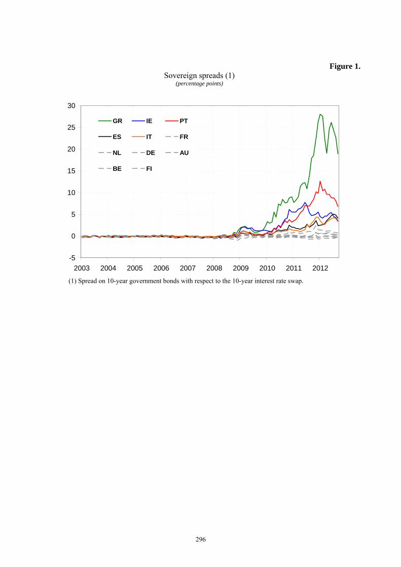
Soon after, sovereign bond yields started to diverge (Figure 1); this pattern became more
pronounced following the onset of the sovereign debt crisis in May 2010, which caused significant
heterogeneity in financial conditions across euro-area countries and more generally in
macroeconomic developments. The underlying causes of the increase in heterogeneity originate in
the accumulation of fiscal, macroeconomic and financial imbalances in several euro area countries
prior to the crisis. When the crisis erupted, the unsustainable nature of these imbalances became
evident.
Changes in banks’ funding conditions have been extremely important to assess the ability of
financial intermediaries to supply credit to the real economy. Figure 2 (top panels) reports the cost
of deposit with agreed maturity up to one year held by households.5 Since the beginning of 2009 the
remuneration on these deposits in core countries remained broadly unchanged although with a
larger dispersion compared to the pre-crisis period. For most of the peripheral countries from 2010
until the end of 2011 the cost of these deposits increased significantly, reflecting banks’ difficulties
4 We decided to keep this Section as brief as possible because there are now uncountable sources (central banks’ websites, academic articles and working papers, newspapers, blogs, etc…) where one can read in great detail the chronology of the events that have characterized the sovereign debt crisis in the euro area. 5 We concentrate on the interest rate paid on deposits with agreed maturity up to one year held by households, rather than an average rate on all deposits, for two main reasons. First, the remuneration on overnight deposits, which represent an important fraction of total deposits, has remained virtually unchanged in most countries. Second, the cost of deposits with agreed maturity, which have represented an important form of stable funding for banks, may well represent the marginal cost of stable funding.
273
in obtaining funding via market sources; throughout 2012 it slightly decreased owing to an
improvement in market confidence, which was partly triggered the cuts in the key ECB interest
rates in November and December 2011, as well as the non-standard monetary policy measures
announced by the ECB in December 2011 (in particular, the two three-year longer-term refinancing
operations) which aimed at further alleviating euro area banks’ funding conditions.
Banks’ funding difficulties in the peripheral countries also adversely affected the financing
conditions to non-financing corporations (NFCs) and to households (HHs). As clearly illustrated in
Figure 2 (middle and bottom panels) the cost of short-term loans to NFCs in the peripheral
countries increased abruptly until the end of 2011; in some cases, namely Greece and Portugal, the
interest rates reached the same levels observed in the third quarter of 2008 when the ECB policy
rates were at their pre-crisis levels. Between May 2010 and December 2011 interest rates on short-
term loans to NFCs increased by, respectively, 225, 140, 250 and 210 basis points in Italy, Spain,
Greece and Portugal while in Germany the increase was remarkably smaller (40 basis points) and
substantially in line with the increase (30 basis points) of the overnight (Eonia, Euro OverNight
Index Average) rate. The interest rates on new loans to households for house purchase followed
similar patterns. In either cases, the time dispersion across peer countries significantly increased
during the sovereign debt crisis. The cost of new loans to HHs for house purchases at floating rate
also increased rapidly in tandem with intensification of sovereign tensions. Only in 2012 the
financing conditions in the peripheral countries became more favorable, still remaining at
significantly higher levels than those observed in core countries.
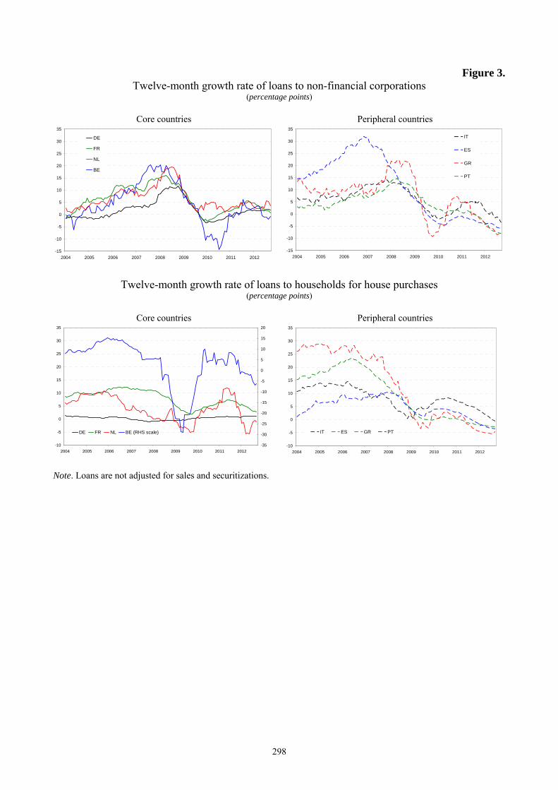
Heterogeneous developments are also detectable when looking at credit developments (Figure
3). Although in 2010 the annual growth of loans to NFCs in core countries followed divergent
patterns, from 2011 onwards growth rates varied in the range 0-5%. In the peripheral countries,
however, despite a generalized recovery in 2010, the annual growth rate of loans to NFCs declined
in 2011 and entered in negative territory in 2012. As for households, loan growth in the peripheral
countries, while most of the correction of past excesses (before the financial crisis loans to
274
households for house purchases grew at double digits in Greece, Spain and Italy) took place in the
period 2006-2009, during the sovereign debt crisis developments in loans to households continued
to remain subdued and in several cases became negative. Developments in lending to NFCs and to
HHs reflected demand as well as supply factors. As for the former one can cite the weakness in
economic activity, in investment spending by firms and housing markets. As for supply factors,
especially towards the end of 2011, access conditions to credit markets tightened substantially in the
peripheral countries. The Bank Lending Survey in the euro area conducted by the Eurosystem
reported a remarkable tightening of credit standards to NFCs as well as the households.
The marked differences in financing conditions across countries and the scarcity of credit in
the peripheral countries have been reflected in a poor economic performance. As reported in Figure
4, while in some core countries industrial production expanded and the unemployment rate either
remained broadly stable or even declined (as in Germany), in the peripheral economies more
affected the sovereign tensions, industrial activity sharply contracted and labour market conditions
deteriorated markedly.6 In most of these countries, industrial production stood at levels reached in
2009. From May 2010 to September 2012, industrial production contracted by 16 per cent in
Greece, 7 in Spain and 3.5 in Italy. In contrast, in Germany as well as in other core countries
industrial production grew by 10 per cent. In the summer of 2011, industrial production in Germany
basically returned to the levels recorded before the 2009 Great Recession; in Italy and Spain,
industrial production was lower by, respectively, 16 and 20 per cent.
Together with the decline in economic activity, the unemployment rate sharply increased in
the peripheral countries, in particular in Greece, Portugal and Spain. In Italy, unemployment started
rising in the summer of 2011.
6 From mid-2009 to the beginning of 2012 unemployment in Germany steadily declined from 8 per cent to 5.5, as a result of the recourse during the crisis to more generous public subsidies and the achievement of agreements at the firm level that ensured employment levels in exchange for wage concessions or arrangements (see the box “Recent developments in the macroeconomic framework in Germany”, in Economic Bulletin of the Bank of Italy, No. 62).
275
4. A Factor Augmented Vector Autoregression (FAVAR) model
In order to assess the effect of the sovereign debt crisis on key macroeconomic variables we
rely on a Factor Augmented Vector Autoregressive (FAVAR) model that allows studying the effect
of shocks on a large set of variables. As thoroughly documented in several recent contributions (e.g.
Bernanke and Boivin, 2003; Bernanke, Boivin and Eliasz, 2005), the FAVAR approach builds on
the idea the information contained in a large number of variables can be accurately captured by a
small number of unobservable factors, which can then be included in a standard VAR model and to
allow for a better characterization of the dynamics of the macroeconomic variables.
In what follows, we briefly go through the main steps of the FAVAR approach, highlighting
some methodological issues we are confronted with.
4.1. Extraction of the factors: A Principal Component Analysis
Let tX denote an ( 1xn ) vector (with xn large) of economic variables for which we want to
assess the dynamic response after a sovereign debt shock (to be defined shortly). To resolve the
dimensionality problem that would make the analysis infeasible, the first step of the FAVAR
approach is to run a Principal Component Analysis (PCA) on tX , obtaining the following
decomposition of tX :7
)1()1()()1(
xffxx nt
nt
nn
F
nt FX (1)
where tF is a vector of unobservable factors (with fn small), t is a vector of idiosyncratic
components and F is a matrix of factor loadings.8 However, since the main goal of our analysis is
to assess the effects of an unanticipated increase in the measure of sovereign debt tensions (see
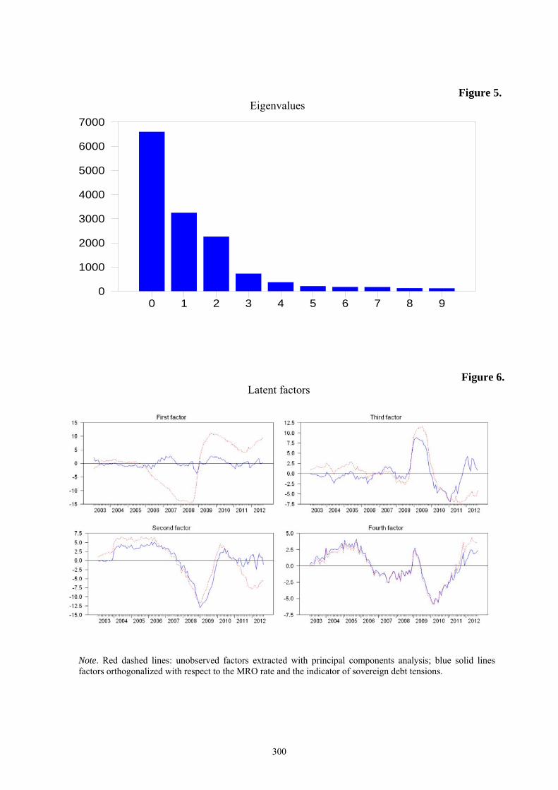
7 The PCA is a statistical technique that is used to determine whether the observed correlation between a given set of variables can be explained by a smaller number of unobserved and unrelated common factors. 8 The number of factors to be retained is chosen on the basis of scree plot of the eigenvalues against the factor numbers. In particular, the number of factors coincides with the number of factors before the plotted line turns flat.
276
section 4.3) and the role of monetary policy we impose some observable factors tY . Formally, the
decomposition of tX now reads
)1()1()()1()()1(
~~~
xyyxffxx nt
nt
nn
Y
nt
nn
F
nt YFX (2)
where Y is a matrix of observable factor loading. Note that in (2) F~ , tF~
and t~
have a
superscript “~”. In particular, the unobserved factors need to be orthogonalised with respect to tY
and thus for this reason tF is replaced by the residual of the following simple linear regression:
ttt FYF~
and a new matrix of factor loading F~ is computed. Consequently, the vector t~
of idiosyncratic
components is also re-computed. Note that these transformations are necessary in order to ensure a
contemporaneous orthogonality between tF~
and tY and thus making it possible to examine the
effects of a shock to a variable in tY onto Ft and thereafter onto tX (Bernanke, Boivin and Eliasz,
2005).9
Throughout our analysis, we assume that vector tY is bi-dimensional and includes the
sovereign debt tensions indicator st (see section 4.3) as well as the monetary policy interest rate rt
(the rate on the main refinancing operations, MRO). The inclusion of the sovereign debt tensions
indicator is trivially dictated by the fact that the scope of our analysis is to examine the effects of a
sovereign debt tensions shock and thus we need have it in tY . There are two reasons why we treat
the monetary policy rate as an observable factor. First, it turns out that one of the factors obtained in
(1) visibly resembles the monetary policy rate or a very short-term money market interest rate. This
is clearly illustrated in Figure 6. We thus have decided to impose the monetary policy rate as an
observable factor. The second reason is that we are interested in studying the response of
9 For this procedure to work one has also to ensure that the idiosyncratic components are orthogonal to tY .

277
conventional monetary policy to the shock. Likewise for this purpose we need have the monetary
policy rate among the observable factors.10
Estimation of the unobserved factors
The unobserved factors are extracted from a series of 139 macroeconomic variables from
January 2003 to September 2012. As for the factors, we decided to use a longer sample period in
order to better capture the co-movements among the variables. On this regard, however, it is worth
noting that the factors estimated over the 2003-2012 period are virtually identical to those estimated
using the shorter 2008-2012 sample.
The set of variables includes industrial production for the total industry excluding
construction, unemployment rates for the whole economy, loans to non-financial corporations, loans
to households for house purchase, interest rates on new loans to non-financial corporations and
households for house purchase at floating rate, interest rates on households deposits with agreed
maturity up to one year, national contributions to the euro area monetary aggregate M3, inflation
rates based on the Harmonized Indices of Consumer Prices (HICP), a group of variables for the
euro area as a whole and, finally, sovereign spreads. The transformation applied to the time series
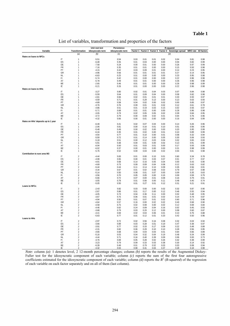
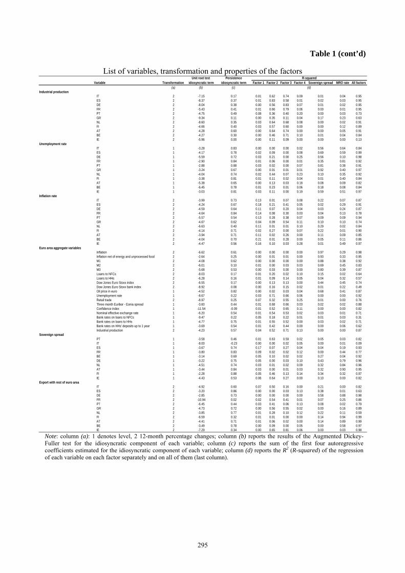
are reported, together with the list of variables, in Table 1.
The transformed data are expressed in deviation from the sample mean and divided by their
sample standard deviation. The number of factors extracted from the cross section of variables Xt
turns out to be four. They account for around 80 per cent of the cross sectional variance. To assess
the goodness of fit of the four latent factors as well as the two observable factors in explaining the
variability of Xt we run linear regressions for each of the variables in Xt on the factors and compute
the R2. As reported in Table 1, the six factors provide a reasonable characterization of the set of
variables with only one exception, industrial production in Ireland. Overall the average R2 is equal
to 0.89 and reaches 0.98 for bank rates, 0.92 for credit, 0.80 for industrial production and 0.91 for
10 If we left the monetary policy rate in the vector Xt and did not include it in the VAR there would not be any feedback effect from the policy rate to the other variables and this in turn would the counterfactual exercise meaningless.
278
the unemployment rate; the R2 for the other categories are between 0.76 and 0.86. Figure 6 reports
both the PCA factors and the orthogonalized ones. Importantly, based on standard unit root tests,
the idiosyncratic components are stationary and this allows us to avoid a detailed investigation on
whether the factors are I(0) or some of them are I(1) (see Bai and Ng, 2004).
Similar results concerning the estimation of the unobserved factors are obtained if one first
removes from all the variables in X the contemporaneous relation with the measure of sovereign
debt tensions as well as with the monetary policy rate and then extracts the latent factors using the
residuals of such regressions (see Buch, Eickmeier and Prieto, 2010).11
4.2. A VAR model
Once we have the unobservable and the observable factors we construct and estimate a
reduced-form p-order VAR model:
tkt
p
kpt ZAz
1
, with zztt zzE ' (3)
where tttt rsFz~ and ts and tr are the two observable factors, the indicator of sovereign debt
tensions and the monetary policy rate, respectively.
In order to ensure identification of structural shocks, we assume – in line also with previous
FAVAR analyses – a Cholesky factorization of the covariance matrix of the reduced-form residuals
'10
'0
AAzz
where the matrix 0A , which describes the contemporaneous relations among the elements of vector
tz , is lower triangular.12 Such a recursive structure implies that the unobservable factors do not
contemporaneously respond to either the sovereign debt tensions or to the monetary policy rate; the 11 We thank Fabio Canova for suggesting this alternative method for estimating the latent factors. The results are available upon request. 12 Sign restrictions are not useful as it is not easy to derive meaningful and theoretically justified restrictions to be imposed on the impulse responses there are only two observable variables, the MRO and the indicator of sovereign debt tensions, the responses of which can be restricted to have given signs.
279
sovereign debt tensions instead does respond contemporaneously to the latent factors but not to the
policy rate; finally, the policy rate is left free to respond contemporaneously to measure of
sovereign debt tensions as well as to the latent factors. Thus, it is clear the importance of ensuring
the contemporaneous orthogonality between tF~
and tY , which then allows use to use the
identification strategy sketched above.13
Estimation of the VAR model
The VAR model is estimated using a Bayesian approach and in particular assuming a normal-
diffuse prior for the coefficients (Kadiyala and Karlsson, 1997). This approach has several
advantages. First, it provides an easier and more accurate assessment of the uncertainty. Second, it
easily allows incorporating a priori information. Third, it better copes with the presence of unit
roots (Sims and Uhlig, 1991). Finally, in-sample over-fitting is less problematic with Bayesian
VAR models which have also good forecasting properties (Doan, Litterman and Sims, 1984).
The VAR model is estimated from January 2008 to September 2012 in order to focus on the
financial turmoil that followed Lehman Brothers’ collapse and on the euro-area sovereign debt
crisis. The order of the VAR is set to 2 based on the Schwarz’s Bayesian information criterion
(BIC) and the outcome of serial correlation tests of the estimated residuals. Inspection of the
residuals does not reveal any sign of heteroskedasticity, which is confirmed by formal tests.
As for the choice of the prior, we rely on the Litterman prior and set the mean of the
coefficients on the first lag of each variable (except the indicator of the sovereign debt tensions) to
0.95, which corresponds to the average of the AR(1) coefficients over the VAR estimation period.14
Given a normal distribution of the error terms in (2), the posterior distribution is normal-Wishart.
Inference is conducted using the Gibbs algorithm.15 Inference on the impulse responses is carried
13 Strictly speaking, since we are interested in the effects of a sovereign debt tensions shock it would be enough to
ensure orthogonality between tF~
and ts . 14 Assuming a unit root prior yields similar results. 15 Draws from the posterior distribution for which the companion of the VAR has eigenvalues larger than one in absolute value are discarded.
280
out with Monte Carlo methods drawing from the posterior distribution (which is normal conditional
on the covariance matrix of the residuals) of the reduced-from parameters and that the covariance
matrix of the residuals (which has a Wishart distribution).
4.3. Measuring the sovereign debt tensions
There exists a vast literature on the identification of structural shocks in VAR models. Just to
name a few, Christiano, Eichenbaum and Evans (1999) have examined the effects of a monetary
policy shock in the U.S. while Galí (1999) have concentrated on technology shocks. While the
literature has converged on a particular set of assumptions for identifying the former shocks, the
identification of an exogenous “sovereign debt tensions” shock is an unchartered territory.
The task of identifying a sovereign debt tensions shock is hard for several reasons. First, the
sovereign debt tensions have materialized in the euro area only in late November 2009, when the
new Greek government disclosed a significant revision to budget deficit and nearly doubled the
2009 forecast to roughly 13 per cent of GDP. Second, the financial turmoil initially confined to
Greece rapidly spread to Ireland, whose economy suffered the consequences of a severe banking
crisis, and to Portugal, whose economy was penalized by a sizable external trade imbalance and
characterized by weak growth prospects. Tensions in financial markets assumed systemic
proportions in the summer of 2011, when the European Council announced the private-sector
involvement (PSI) to resolve the Greek crisis. Financial tensions then quickly passed onto Italian
and Spanish government bonds. The Spanish economy was weakened by the burst of a housing
bubble and by a fragile banking sector while the Italian economy was held back by weak prospects
of economic growth and by an extremely high level of public debt to GDP ratio.
Figure 1 plots the 10-year sovereign spreads for the major euro-area countries. The spreads are
computed with respect to the 10-year interest swap rate in order to account for flight-to-quality
effects towards the German Bund during the financial and sovereign debt crises (De Sanctis, 2012).
From 2003 to mid-2009, the average 10-year sovereign spread ranged from 22 basis points for
281
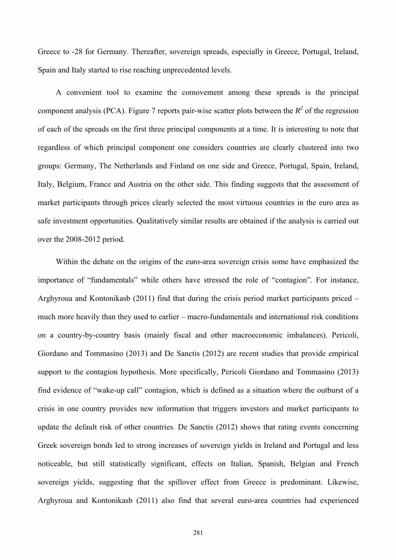
Greece to -28 for Germany. Thereafter, sovereign spreads, especially in Greece, Portugal, Ireland,
Spain and Italy started to rise reaching unprecedented levels.
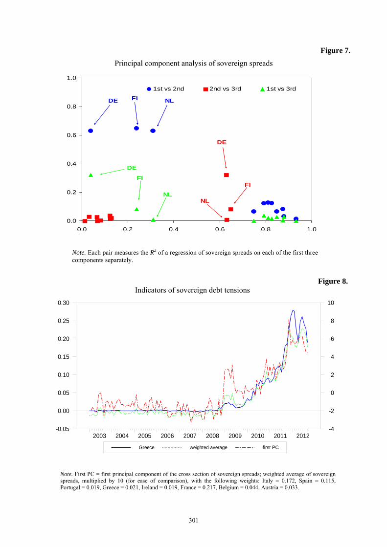
A convenient tool to examine the comovement among these spreads is the principal
component analysis (PCA). Figure 7 reports pair-wise scatter plots between the R2 of the regression
of each of the spreads on the first three principal components at a time. It is interesting to note that
regardless of which principal component one considers countries are clearly clustered into two
groups: Germany, The Netherlands and Finland on one side and Greece, Portugal, Spain, Ireland,
Italy, Belgium, France and Austria on the other side. This finding suggests that the assessment of
market participants through prices clearly selected the most virtuous countries in the euro area as
safe investment opportunities. Qualitatively similar results are obtained if the analysis is carried out
over the 2008-2012 period.
Within the debate on the origins of the euro-area sovereign crisis some have emphasized the
importance of “fundamentals” while others have stressed the role of “contagion”. For instance,
Arghyroua and Kontonikasb (2011) find that during the crisis period market participants priced –
much more heavily than they used to earlier – macro-fundamentals and international risk conditions
on a country-by-country basis (mainly fiscal and other macroeconomic imbalances). Pericoli,
Giordano and Tommasino (2013) and De Sanctis (2012) are recent studies that provide empirical
support to the contagion hypothesis. More specifically, Pericoli Giordano and Tommasino (2013)
find evidence of “wake-up call” contagion, which is defined as a situation where the outburst of a
crisis in one country provides new information that triggers investors and market participants to
update the default risk of other countries. De Sanctis (2012) shows that rating events concerning
Greek sovereign bonds led to strong increases of sovereign yields in Ireland and Portugal and less
noticeable, but still statistically significant, effects on Italian, Spanish, Belgian and French
sovereign yields, suggesting that the spillover effect from Greece is predominant. Likewise,
Arghyroua and Kontonikasb (2011) also find that several euro-area countries had experienced

282
contagion from Greece supporting the view that Greek bond yield has become a proxy for EMU-
specific systemic risk, increasing borrowing costs in other EMU countries beyond the level justified
by the common international risk factor and their idiosyncratic fundamentals.16
In light of the above considerations, the following measures of sovereign debt tensions are
used in the estimation of the VAR: (i) the spread between the 10-year Greek bonds yield and the 10-
year interest rate swap, based on the evidence of “wake-up call” contagion; (ii) the weighted
average of the spreads between the 10-year Italian, Greek, Irish, Portuguese, Spanish, Belgian,
French and Austrian bonds yields and the 10-year interest rate swap, based on the results of the
PCA reported in Figure 7; (iii) the first principal component on the whole set of sovereign spreads.
Figure 8 shows our three indicators. Interestingly, they show remarkably similar patterns as also
confirmed by the large pair-wise correlations (between 0.90 and 0.98).
5. The macroeconomic effects of the sovereign debt crisis
In this Section we describe the impulse responses of the macroeconomic variables to a
sovereign tensions shock, identified using the Greek spread as measure of the tensions, and with the
FAVAR outlined in Section 4.1 and employing the identification strategy discussed in Section 4.2.
In particular, we examine the effects of an unexpected increase of 350 basis points in the Greek
spread, which roughly corresponds to the increase observed from August to September 2011 after
the announcement of the PSI. The results obtained using the other two indicators of the sovereign
tensions are discussed in the Section 5.3.
16 Several recent studies have put forward theoretical models with the aim to shed light on the possible causes and propagations mechanisms of the sovereign debt crisis in the euro area. For example, Arghyrou and Tsoukalas (2010) develop a theoretical model of the euro-area sovereign debt crisis combining elements from the second- and third generation currency crisis models, by Obstfeld (1996) and Krugman (1979) respectively. Guerrieri, Iacoviello and Minetti (2012) examine the international propagation of a sovereign debt default in a two-country microfounded economic model calibrated to data from the euro area, with the two countries representing the periphery (Greece, Italy, Portugal and Spain) and the core.
283
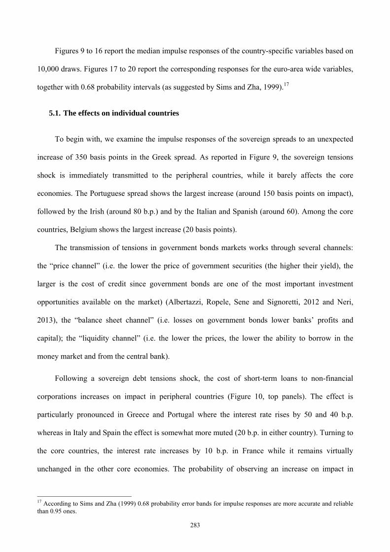
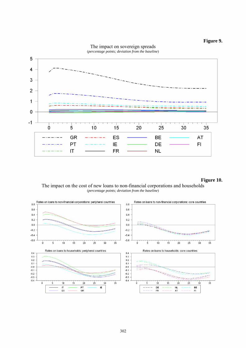
Figures 9 to 16 report the median impulse responses of the country-specific variables based on
10,000 draws. Figures 17 to 20 report the corresponding responses for the euro-area wide variables,
together with 0.68 probability intervals (as suggested by Sims and Zha, 1999).17
5.1. The effects on individual countries
To begin with, we examine the impulse responses of the sovereign spreads to an unexpected
increase of 350 basis points in the Greek spread. As reported in Figure 9, the sovereign tensions
shock is immediately transmitted to the peripheral countries, while it barely affects the core
economies. The Portuguese spread shows the largest increase (around 150 basis points on impact),
followed by the Irish (around 80 b.p.) and by the Italian and Spanish (around 60). Among the core
countries, Belgium shows the largest increase (20 basis points).
The transmission of tensions in government bonds markets works through several channels:
the “price channel” (i.e. the lower the price of government securities (the higher their yield), the
larger is the cost of credit since government bonds are one of the most important investment
opportunities available on the market) (Albertazzi, Ropele, Sene and Signoretti, 2012 and Neri,
2013), the “balance sheet channel” (i.e. losses on government bonds lower banks’ profits and
capital); the “liquidity channel” (i.e. the lower the prices, the lower the ability to borrow in the
money market and from the central bank).
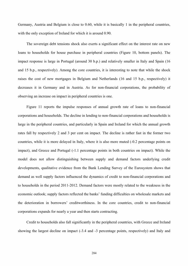
Following a sovereign debt tensions shock, the cost of short-term loans to non-financial
corporations increases on impact in peripheral countries (Figure 10, top panels). The effect is
particularly pronounced in Greece and Portugal where the interest rate rises by 50 and 40 b.p.
whereas in Italy and Spain the effect is somewhat more muted (20 b.p. in either country). Turning to
the core countries, the interest rate increases by 10 b.p. in France while it remains virtually
unchanged in the other core economies. The probability of observing an increase on impact in
17 According to Sims and Zha (1999) 0.68 probability error bands for impulse responses are more accurate and reliable than 0.95 ones.
284
Germany, Austria and Belgium is close to 0.60, while it is basically 1 in the peripheral countries,
with the only exception of Ireland for which it is around 0.90.
The sovereign debt tensions shock also exerts a significant effect on the interest rate on new
loans to households for house purchase in peripheral countries (Figure 10, bottom panels). The
impact response is large in Portugal (around 30 b.p.) and relatively smaller in Italy and Spain (16
and 15 b.p., respectively). Among the core countries, it is interesting to note that while the shock
raises the cost of new mortgages in Belgium and Netherlands (16 and 15 b.p., respectively) it
decreases it in Germany and in Austria. As for non-financial corporations, the probability of
observing an increase on impact in peripheral countries is one.
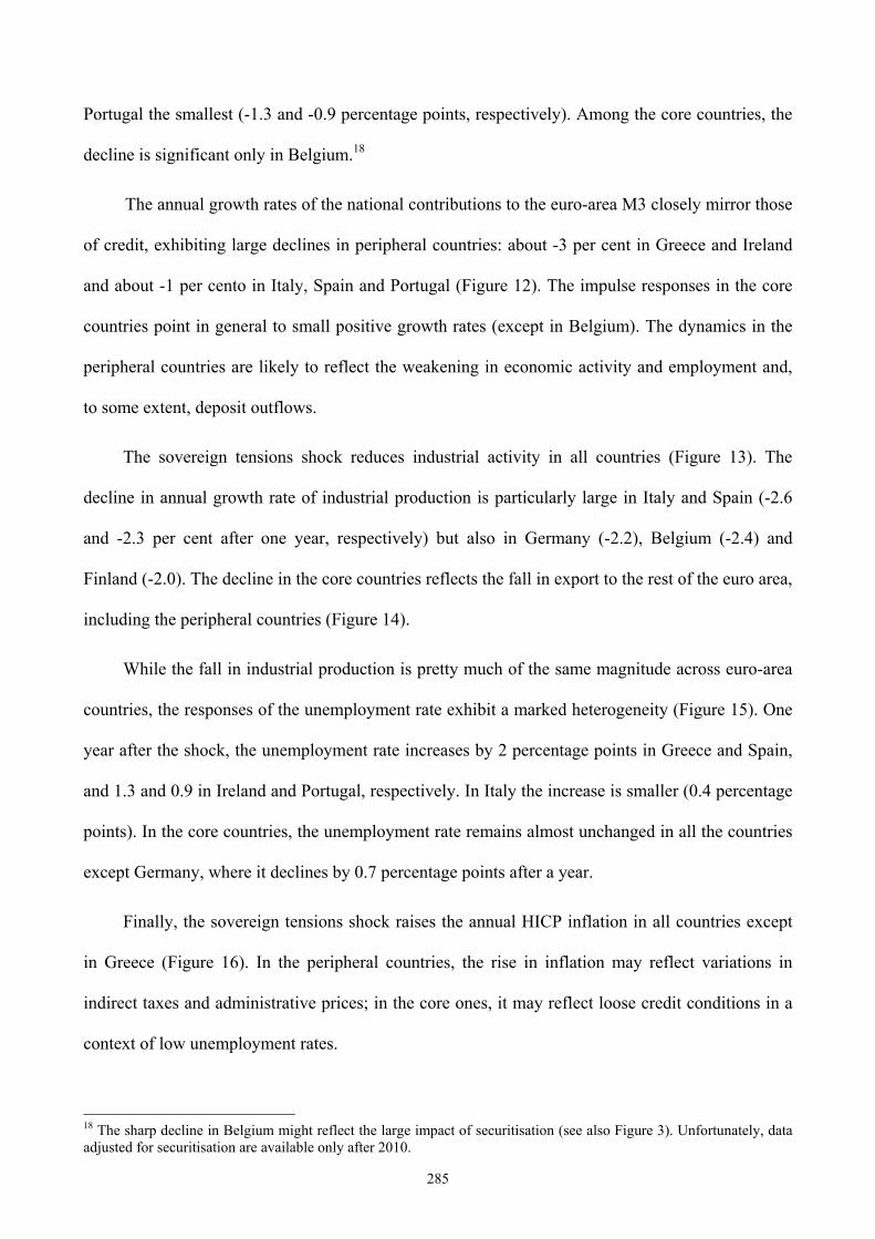
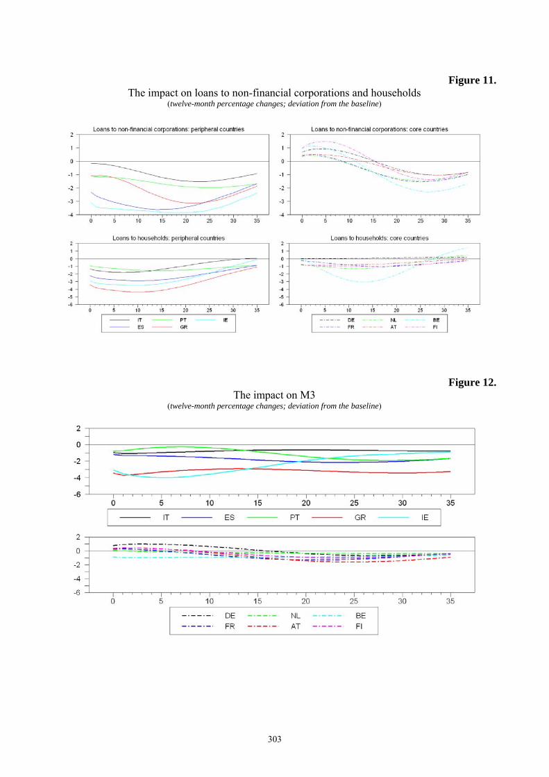
Figure 11 reports the impulse responses of annual growth rate of loans to non-financial
corporations and households. The decline in lending to non-financial corporations and households is
large in the peripheral countries, and particularly in Spain and Ireland for which the annual growth
rates fall by respectively 2 and 3 per cent on impact. The decline is rather fast in the former two
countries, while it is more delayed in Italy, where it is also more muted (-0.2 percentage points on
impact), and Greece and Portugal (-1.1 percentage points in both countries on impact). While the
model does not allow distinguishing between supply and demand factors underlying credit
developments, qualitative evidence from the Bank Lending Survey of the Eurosystem shows that
demand as well supply factors influenced the dynamics of credit to non-financial corporations and
to households in the period 2011-2012. Demand factors were mostly related to the weakness in the
economic outlook; supply factors reflected the banks’ funding difficulties on wholesale markets and
the deterioration in borrowers’ creditworthiness. In the core countries, credit to non-financial
corporations expands for nearly a year and then starts contracting.
Credit to households also fall significantly in the peripheral countries, with Greece and Ireland
showing the largest decline on impact (-3.4 and -3 percentage points, respectively) and Italy and
285
Portugal the smallest (-1.3 and -0.9 percentage points, respectively). Among the core countries, the
decline is significant only in Belgium.18
The annual growth rates of the national contributions to the euro-area M3 closely mirror those
of credit, exhibiting large declines in peripheral countries: about -3 per cent in Greece and Ireland
and about -1 per cento in Italy, Spain and Portugal (Figure 12). The impulse responses in the core
countries point in general to small positive growth rates (except in Belgium). The dynamics in the
peripheral countries are likely to reflect the weakening in economic activity and employment and,
to some extent, deposit outflows.
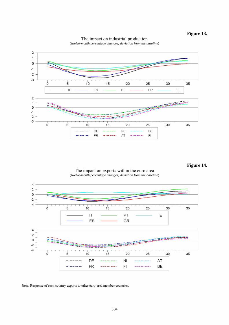
The sovereign tensions shock reduces industrial activity in all countries (Figure 13). The
decline in annual growth rate of industrial production is particularly large in Italy and Spain (-2.6
and -2.3 per cent after one year, respectively) but also in Germany (-2.2), Belgium (-2.4) and
Finland (-2.0). The decline in the core countries reflects the fall in export to the rest of the euro area,
including the peripheral countries (Figure 14).
While the fall in industrial production is pretty much of the same magnitude across euro-area
countries, the responses of the unemployment rate exhibit a marked heterogeneity (Figure 15). One
year after the shock, the unemployment rate increases by 2 percentage points in Greece and Spain,
and 1.3 and 0.9 in Ireland and Portugal, respectively. In Italy the increase is smaller (0.4 percentage
points). In the core countries, the unemployment rate remains almost unchanged in all the countries
except Germany, where it declines by 0.7 percentage points after a year.
Finally, the sovereign tensions shock raises the annual HICP inflation in all countries except
in Greece (Figure 16). In the peripheral countries, the rise in inflation may reflect variations in
indirect taxes and administrative prices; in the core ones, it may reflect loose credit conditions in a
context of low unemployment rates.
18 The sharp decline in Belgium might reflect the large impact of securitisation (see also Figure 3). Unfortunately, data adjusted for securitisation are available only after 2010.
286
To sum up, an unexpected increase in sovereign debt tensions leads a rise in sovereign spreads
of all the peripheral countries and to significantly heterogeneous credit conditions and credit
dynamics across countries. The impact on industrial activity is similar across countries, possibly
reflecting the strong trade links. The diverging responses in the unemployment may be related to
structural differences in labour markets, including job protection and labour market flexibility.
The next Section discusses the impact on euro-area aggregate variables.
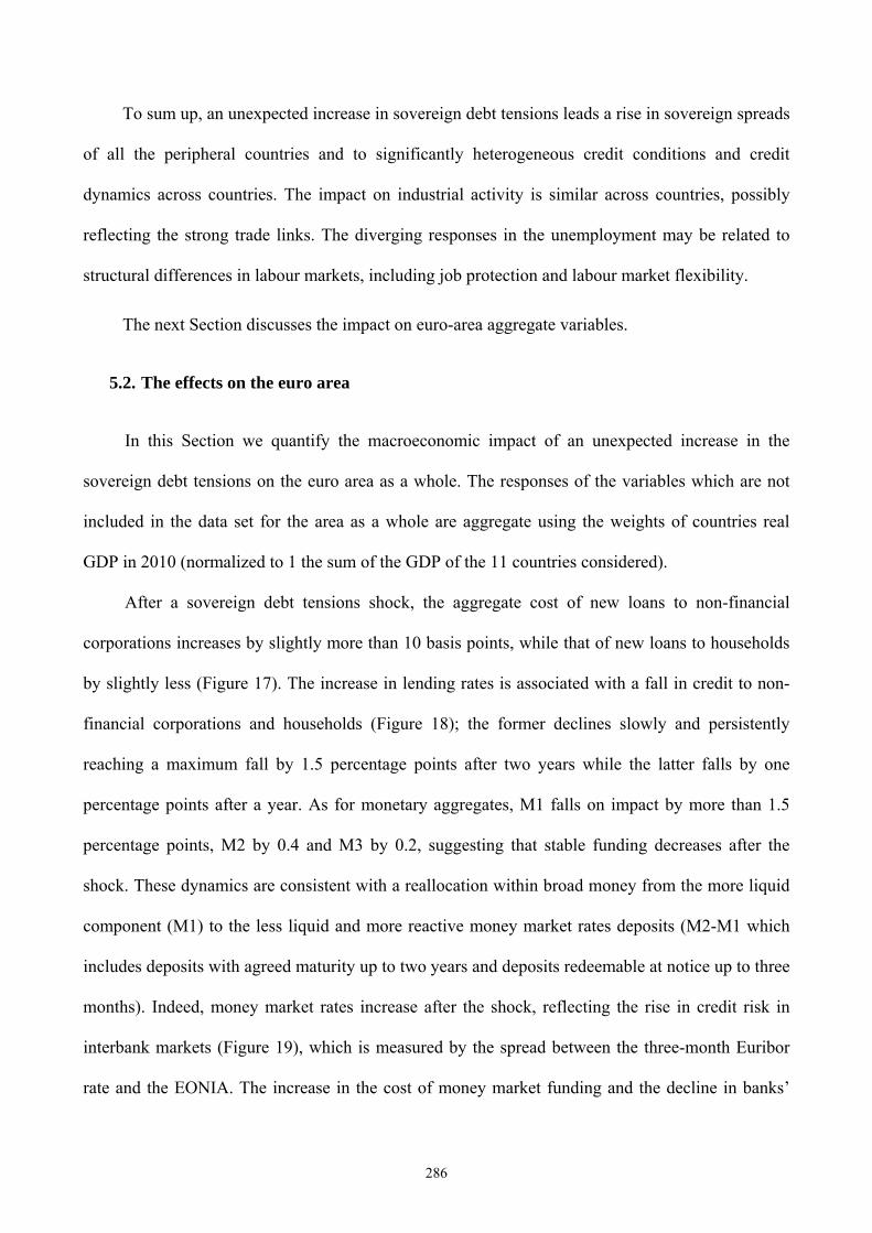
5.2. The effects on the euro area
In this Section we quantify the macroeconomic impact of an unexpected increase in the
sovereign debt tensions on the euro area as a whole. The responses of the variables which are not
included in the data set for the area as a whole are aggregate using the weights of countries real
GDP in 2010 (normalized to 1 the sum of the GDP of the 11 countries considered).
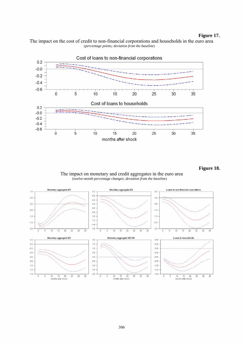
After a sovereign debt tensions shock, the aggregate cost of new loans to non-financial
corporations increases by slightly more than 10 basis points, while that of new loans to households
by slightly less (Figure 17). The increase in lending rates is associated with a fall in credit to non-
financial corporations and households (Figure 18); the former declines slowly and persistently
reaching a maximum fall by 1.5 percentage points after two years while the latter falls by one
percentage points after a year. As for monetary aggregates, M1 falls on impact by more than 1.5
percentage points, M2 by 0.4 and M3 by 0.2, suggesting that stable funding decreases after the
shock. These dynamics are consistent with a reallocation within broad money from the more liquid
component (M1) to the less liquid and more reactive money market rates deposits (M2-M1 which
includes deposits with agreed maturity up to two years and deposits redeemable at notice up to three
months). Indeed, money market rates increase after the shock, reflecting the rise in credit risk in
interbank markets (Figure 19), which is measured by the spread between the three-month Euribor
rate and the EONIA. The increase in the cost of money market funding and the decline in banks’
287
stable funding exert a negative impact on banks’ profitability as shown by the large decline in the
average price of banks’ stocks.
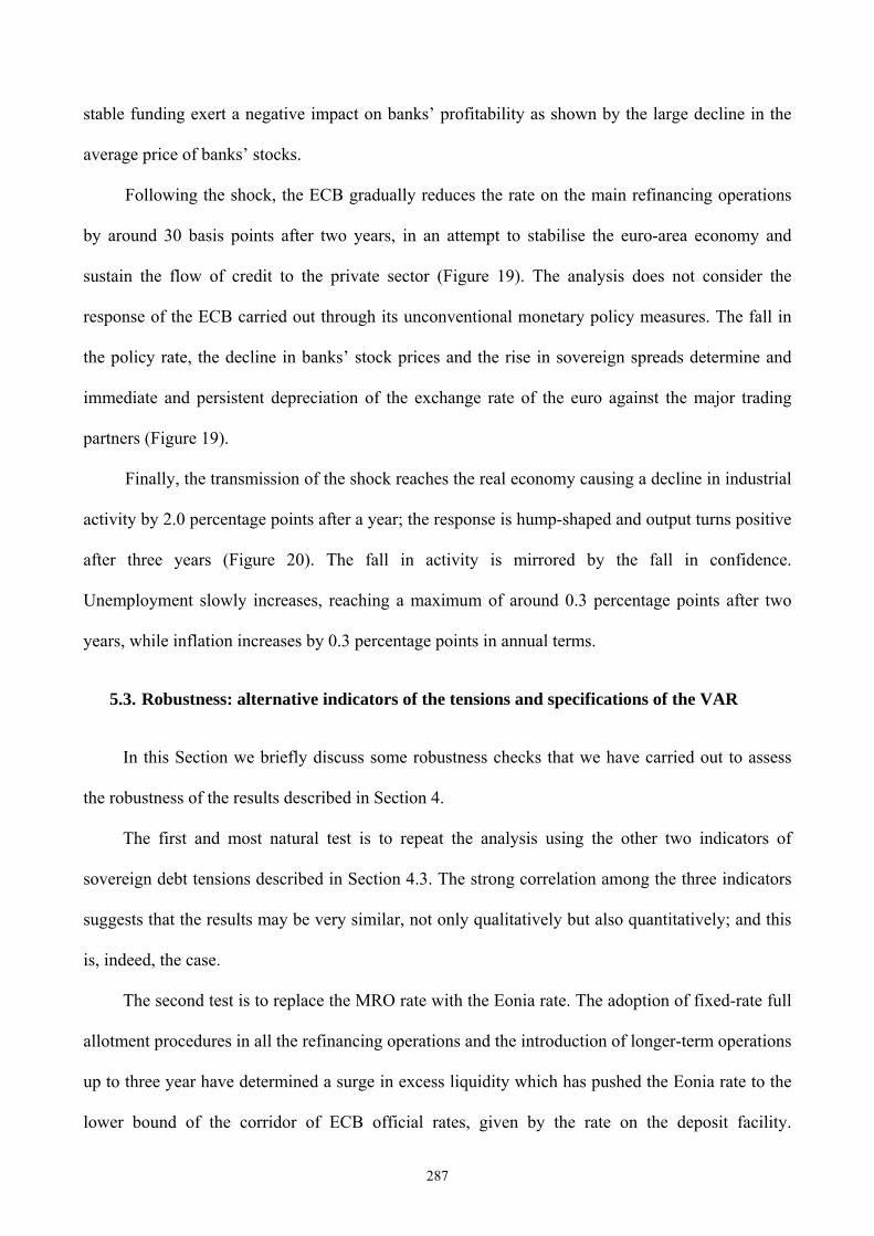
Following the shock, the ECB gradually reduces the rate on the main refinancing operations
by around 30 basis points after two years, in an attempt to stabilise the euro-area economy and
sustain the flow of credit to the private sector (Figure 19). The analysis does not consider the
response of the ECB carried out through its unconventional monetary policy measures. The fall in
the policy rate, the decline in banks’ stock prices and the rise in sovereign spreads determine and
immediate and persistent depreciation of the exchange rate of the euro against the major trading
partners (Figure 19).
Finally, the transmission of the shock reaches the real economy causing a decline in industrial
activity by 2.0 percentage points after a year; the response is hump-shaped and output turns positive
after three years (Figure 20). The fall in activity is mirrored by the fall in confidence.
Unemployment slowly increases, reaching a maximum of around 0.3 percentage points after two
years, while inflation increases by 0.3 percentage points in annual terms.
5.3. Robustness: alternative indicators of the tensions and specifications of the VAR
In this Section we briefly discuss some robustness checks that we have carried out to assess
the robustness of the results described in Section 4.
The first and most natural test is to repeat the analysis using the other two indicators of
sovereign debt tensions described in Section 4.3. The strong correlation among the three indicators
suggests that the results may be very similar, not only qualitatively but also quantitatively; and this
is, indeed, the case.
The second test is to replace the MRO rate with the Eonia rate. The adoption of fixed-rate full
allotment procedures in all the refinancing operations and the introduction of longer-term operations
up to three year have determined a surge in excess liquidity which has pushed the Eonia rate to the
lower bound of the corridor of ECB official rates, given by the rate on the deposit facility.

288
Therefore, the Eonia partly reflects changes in the MRO, and more precisely in the rate on the
deposit facility, and partly the effects of the unconventional measures. Also in this case, the results
are qualitatively similar.
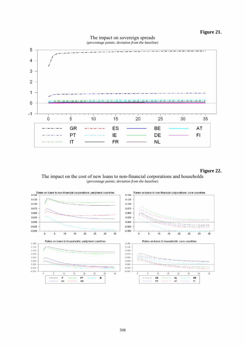
The third test is to perform the analysis using the three-month differences for the variables
which have been transformed using twelve-month changes and first differences for unemployment,
lending rates and the sovereign spreads.19 The results, which are broadly in line with those
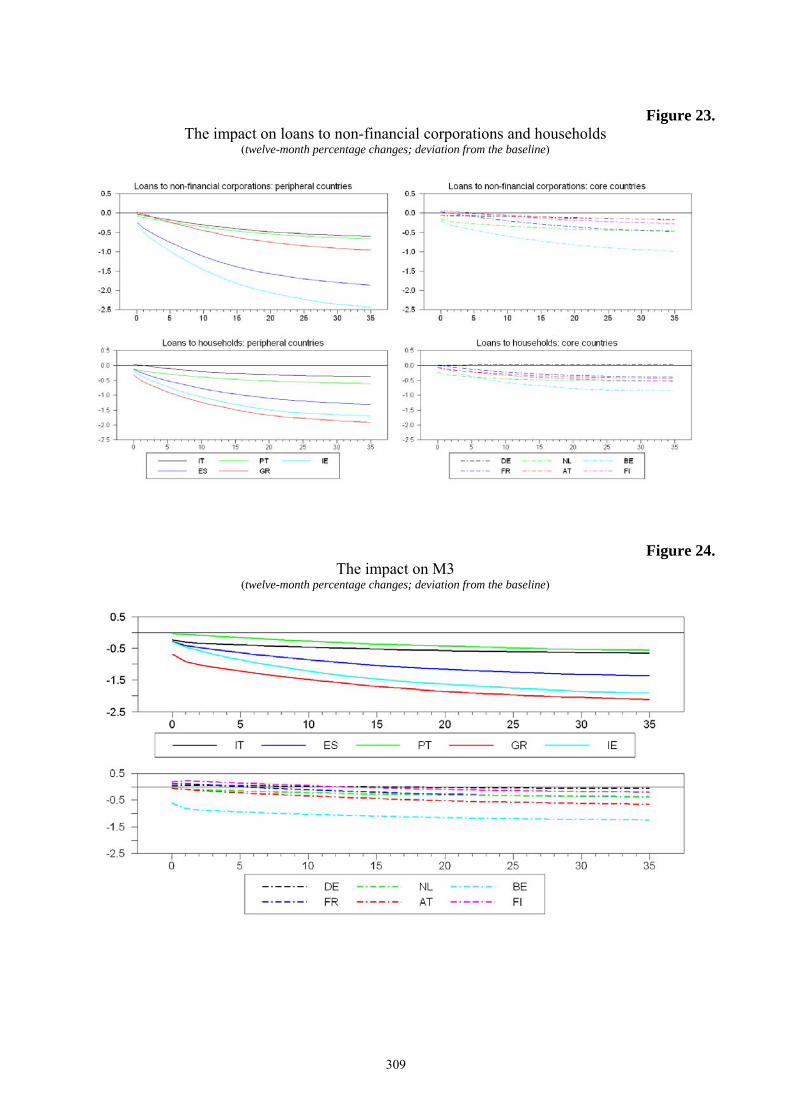
discussed in the previous sections, are reported in Figure 21 to 30. The results are broadly in line
with those obtained with the baseline model and discussed in Sections 5.1 and 5.2. The larger
persistence that characterizes almost all the responses is due to the transformation of the variables.
Bank rates increase and lending and M3 fall substantially in the peripheral countries (Figures 22, 23
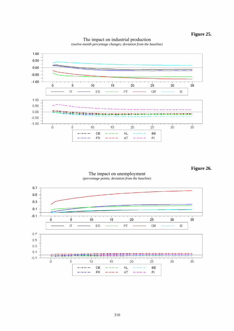
and 24) The fall in industrial production is more muted in Italy and Spain as well as in the core
countries (Figure 25). Unemployment increases sharply in Greece while does not respond in the
core countries (Figure 26). The increase in the other peripheral countries is smaller than in the
baseline model. As for the aggregate variables, the impulse responses are in line with the baseline
results (Figures 27 to 30). The only qualitative difference arises for the response of the nominal
exchange rate, which appreciates following the sovereign shock.
Fourth, we have introduced the debt-to GDP ratios in the set of variables Xt. This has the
advantage of allowing assessing the impact of the sovereign tensions on public debt and better
identifying the sovereign tension shock by taking into account a key determinant of sovereign
spreads (see, among others, Pericoli, Giordano and Tommasino, 2012). Overall, the impulse
responses do not change. The responses of the debt-to-GDP ratios (Figure 31) are in line with our
expectations; the peripheral countries experience a rapid increase while core countries are basically
unaffected. In particular, public debt increases sharply in Ireland (by 12 percentage points), Portugal
and Greece (8 percentage points), and slightly less in Spain and Italy (4 and 2, respectively).
Finally, we have estimated the VAR over the period 2003:1-2007:12 and found, in line with our
19 The exchange rate and the Euribor-Eonia swap spread enter in level while oil prices are first-differenced.
289
expectations, that an unexpected increase in sovereign spreads does not have exert any visible effect
on any of the macroeconomic variables.
6. Conclusions
Almost four years have passed since the outburst of the global financial crisis, the euro area is
struggling with an unprecedented crisis that has its roots, on the one hand, in the weak fiscal
positions and macroeconomic imbalances of the peripheral countries and, on the other hand, in the
lack of adequate instruments for managing and resolving the crisis, coupled with the incompleteness
of the euro area architecture. The strong interconnection between sovereigns and banks has been a
powerful transmission mechanism of the tensions in government bond markets. Two years and a
half after the beginning of the tensions in government bond markets, economic activity is
weakening in all euro-area member countries.
Surprisingly enough, there is very little evidence on the macroeconomic impact of the
sovereign debt crisis on the euro area as a whole and on the individual countries. The aim of our
research, which has to be though of as a starting point for a more structural analysis, is to fill this
gap by resorting on state-of-the-art econometric tools, known as Factor Augmented Vector
Autoregressive (FAVAR) models.
The empirical analysis confirms that the crisis, that started at the end of 2009 in Greece,
rapidly spread to other countries with weak fiscal and macroeconomic conditions, namely Portugal
and Ireland, and with some delay to Spain, which had suffered the consequences of a fall in
property prices, and Italy, with its high public debt and weak growth prospects in the medium term.
Credit conditions have become significantly heterogeneous, with the cost of credit raising sharply in
the peripheral countries, and posing important challenges to the ECB monetary policy. The tensions
in sovereign debt markets have caused a decline in economic activity in all countries and also at the
aggregate euro-area level.
290
While our analysis helps understanding the real effects of the sovereign crisis, a lot more
needs to be done, in particular along two dimensions. On the empirical side, more elaborated
models, possibly allowing for time variation in parameters (Primiceri, 2005 and Koop and
Korobilis, 2012), might be more useful to complete our task to fully capture the transmission of the
sovereign debt crisis to the euro-area economy. The Large Bayesian VAR approach suggested by
by Bańbura, Giannone and Reichlin (forthcoming) is an interesting and appealing alternative to deal
with the high dimension of the data. On the theoretical side, structural models with open economy
features allowing for the possibility of sovereigns’ and banks’ defaults may be extremely useful to
analyse the channels through which the fear of unsustainable fiscal dynamics end up hitting the real
economy and spilling over to the rest of the global economy. Needless to say, such models need to
incorporate not only a “conventional” role for monetary policy but, most importantly, its
“unconventional” dimension.
291
References
Albertazzi, U., T. Ropele, G. Sene and F. M. Signoretti (2012), “The impact of the sovereign debt
crisis on the activity of Italian banks”, Occasional Papers Banca d’Italia, No. 133.
Arghyrou, M. G. and J. Tsoukalas (2011), “The EMU sovereign-debt crisis: Fundamentals,
expectations and contagion”. European Economy - Economic Papers 436, European Commission.
Bai, J. and S. Ng (2004), “A PANIC attack on unit roots and cointegration”, Econometrica, Vol.
72, pp. 1127-1177.
Bańbura, M., D. Giannone, L. Reichlin (2013), “Large Bayesian VARs”, Journal of Applied
Econometrics, forthcoming.
Bank of Italy (2010), Economic Bulletin, No. 62.
Bernanke, B. and J. Boivin (2003), “Monetary Policy in a Data-Rich Environment”, Journal of
Monetary Economics, Vol. 50, pp. 525-546.
Bernanke, B., J. Boivin, and P. Eliasz (2005), “Measuring the Effects of Monetary Policy: A actor-
Augmented Vector Autoregressive (FAVAR) Approach”, The Quarterly Journal of Economics,
Vol. 120(1), pp. 387-422.
Buch, C., S. Eickmeier, and E. Prieto (2010), “Macroeconomic factors and micro-level bank risk”,
Deutsche Bundesbank Discussion Paper, No. 2010/20.
Christiano L. J., M. Eichenbaum M. and C. L. Evans (1999), “Monetary policy shocks: what have
we learned and to what end?”, in Handbook of Macroeconomics, Vol. 1, Ch. 2, Taylor J. B., M.
Woodford (eds), pp. 65-148.
Committee on the Global Financial System (CGFS) (2011), “The impact of sovereign credit risk on
bank funding conditions”, Report submitted by a Study Group established by the Committee on the
Global Financial System, CGFS papers, No. 43.
De Paoli, B., Hoggarth, G. and V. Saporta (2009), “Output costs of sovereign crises: some
empirical estimates”, Bank of England Working Paper, No. 362.
De Santis, R. (2012), “The euro area sovereign debt crisis: Safe haven, credit rating agencies and
the spread of the fever from Greece, Ireland and Portugal”, ECB Working Paper, No. 1419.
292
Doan, T., R. Litterman and C. A. Sims (1984), “Forecasting and conditional projections using
realist prior distributions”, Econometric Review, Vol. 3, pp. 1-100.
Furceri, D. and A. Zdzienicka (2012), “How costly are debt crises?”, Journal of International
Money and Finance, Vol. 31(4), pp. 726-742.
Galí, J. (1999), “Technology, employment, and the business cycle: Do technology shocks explain
aggregate fluctuations?”, American Economic Review, Vol. 89, pp. 249-271.
Guerrieri L, M. Iacoviello and R. Minetti (2012), “Banks, sovereign debt and the international
transmission of business cycles.” International Finance Discussion Papers 1067, Board of
Governors of the Federal Reserve System.
Kadiyala, K. R. and S. Karlsson (1997), “Numerical methods for estimation and inference in
bayesian var-models”, Journal of Applied Econometrics, Vol. 12, pp. 99-132.
Koop, G. and D. Korobilis (2012), “Large time-varying parameter VARs”, The Rimini Centre for
Economic Analysis, Working Paper, No. 12-11.
Krugman, P. R. (1979), “A model of balance of payments crises”, Journal of Money Credit and
Banking, Vol. 11, pp. 311-25.
Neri, S. (2013), “The impact of the sovereign debt crisis on bank lending rates in the euro area”,
mimeo, Banca d’Italia.
Obstfeld, M. (1996), “Models of currency crises with self-fulfilling features”, European Economic
Review, Vol. 40, pp. 1037-48.
Pericoli, M. R. Giordano and P. Tommasino (2013), “‘’Pure’’ or ‘’wake-up-call’’ contagion?
Another look at the EMU sovereign debt crisis”, mimeo, Banca d’Italia.
Primiceri, G. (2005), “Time Varying Structural Vector Autoregressions and Monetary Policy”, The
Review of Economic Studies, Vol. 72, pp. 821-852.
Reinhart, C. M. and K. S. Rogoff (2009), This Time Is Different: Eight Centuries of Financial
Folly. Princeton, NJ: Princeton University Press.
Richmond, C. and D. Dias (2008), “Duration of Capital Market Exclusion: Stylized Facts and
Determining Factors”, mimeo, UCLA.
Rose, A. K. (2005), “One Reason Countries Pay Their Debts: Renegotiation and International
Trade”, Journal of Development Economics, Vol. 77(1), pp. 189-206.

293
Sims, C. A. and H. Uhlig (1991), “Understanding Unit Rooters: A Helicopter Tour”,
Econometrica, Vol. 59, pp. 1591-1599.
Sims, C. A. and T. Zha (1999), “Error bands for impulse responses”, Econometrica, Vol. 67, pp.
1113-1156.
294
Table 1
List of variables, transformation and properties of the factors
Unit root test PersistenceTransformation idiosyncratic term idiosyncratic term Factor 1 Factor 2 Factor 3 Factor 4 Sovereign spread MRO rate All factors
(a) (b) (c)Rates on loans to NFCs
IT 1 -5.51 0.54 0.03 0.01 0.01 0.02 0.04 0.81 0.98ES 1 -6.48 0.35 0.01 0.04 0.00 0.00 0.04 0.82 0.99DE 1 -7.58 0.24 0.00 0.01 0.00 0.00 0.26 0.97 0.99FR 1 -7.16 0.35 0.01 0.01 0.00 0.00 0.15 0.93 0.98PT 1 -4.15 0.42 0.03 0.09 0.01 0.00 0.14 0.23 0.95GR 1 -4.96 0.56 0.01 0.01 0.01 0.01 0.27 0.14 0.95NL 1 -6.63 0.25 0.01 0.00 0.00 0.00 0.20 0.95 0.98FI 1 -5.74 0.42 0.01 0.00 0.00 0.00 0.22 0.96 0.98AT 1 -5.78 0.49 0.01 0.01 0.00 0.00 0.26 0.96 0.98BE 1 -2.65 0.46 0.01 0.01 0.00 0.00 0.26 0.98 0.99IE 1 -5.21 0.26 0.01 0.00 0.00 0.00 0.22 0.96 0.98
Rates on loans to HHsIT 1 -3.27 0.80 0.02 0.01 0.04 0.03 0.07 0.84 0.98ES 1 -5.59 0.64 0.01 0.09 0.04 0.00 0.08 0.82 0.98DE 1 -2.81 0.66 0.02 0.01 0.01 0.01 0.33 0.93 0.97FR 1 -4.59 0.71 0.01 0.29 0.13 0.00 0.13 0.63 0.93PT 1 -4.89 0.58 0.04 0.02 0.00 0.02 0.00 0.65 0.97GR 1 -3.76 0.76 0.09 0.01 0.01 0.02 0.12 0.61 0.78NL 1 -4.86 0.51 0.01 0.19 0.03 0.15 0.02 0.56 0.97FI 1 -5.71 0.68 0.01 0.01 0.00 0.00 0.28 0.96 0.98AT 1 -3.05 0.79 0.02 0.05 0.05 0.02 0.39 0.84 0.95BE 1 -3.72 0.79 0.00 0.09 0.02 0.01 0.04 0.76 0.96IE 1 -4.32 0.66 0.00 0.01 0.00 0.00 0.16 0.94 0.99
Rates on HHs' deposits up to 1 year IT 1 -6.48 0.41 0.02 0.07 0.04 0.00 0.14 0.26 0.96ES 1 -2.06 0.81 0.00 0.16 0.01 0.10 0.01 0.56 0.95DE 1 -5.48 0.49 0.00 0.02 0.00 0.00 0.20 0.95 0.99FR 1 -6.16 0.35 0.01 0.02 0.00 0.01 0.10 0.89 0.99PT 1 -4.54 0.77 0.01 0.10 0.00 0.01 0.08 0.32 0.94GR 1 -5.59 0.72 0.01 0.14 0.00 0.05 0.30 0.06 0.93NL 1 -5.18 0.51 0.00 0.12 0.03 0.04 0.02 0.65 0.93FI 1 -5.91 0.48 0.00 0.01 0.00 0.02 0.13 0.91 0.99AT 1 -6.04 0.50 0.01 0.03 0.01 0.00 0.17 0.93 0.99BE 1 -6.02 0.37 0.00 0.01 0.00 0.00 0.31 0.98 0.99IE 1 -5.76 0.52 0.00 0.04 0.00 0.02 0.04 0.81 0.98
Contribution to euro area M3IT 2 -4.44 0.83 0.01 0.00 0.10 0.01 0.60 0.34 0.78ES 2 -4.08 0.65 0.00 0.01 0.03 0.07 0.51 0.77 0.97DE 2 -4.91 0.68 0.14 0.16 0.05 0.04 0.00 0.43 0.90FR 2 -4.69 0.73 0.09 0.09 0.04 0.08 0.12 0.63 0.82PT 2 -5.44 0.44 0.11 0.14 0.10 0.09 0.35 0.56 0.91GR 2 -4.34 0.67 0.01 0.02 0.08 0.02 0.79 0.57 0.98NL 2 -5.14 0.50 0.08 0.01 0.07 0.00 0.09 0.35 0.63FI 2 -3.56 0.70 0.05 0.05 0.00 0.15 0.09 0.59 0.79AT 2 -5.66 0.72 0.07 0.00 0.01 0.08 0.16 0.79 0.91BE 2 -3.55 0.78 0.01 0.06 0.00 0.11 0.48 0.40 0.74IE 2 -5.05 0.50 0.01 0.27 0.01 0.12 0.31 0.21 0.91
Loans to NFCsIT 2 -2.43 0.82 0.03 0.00 0.00 0.02 0.32 0.87 0.90ES 2 -2.67 0.86 0.01 0.17 0.00 0.12 0.46 0.55 0.94DE 2 -4.05 0.73 0.04 0.36 0.11 0.00 0.02 0.48 0.95FR 2 -3.67 0.75 0.06 0.01 0.01 0.02 0.14 0.78 0.87PT 2 -4.94 0.50 0.01 0.07 0.01 0.02 0.60 0.71 0.96GR 2 -4.64 0.57 0.16 0.00 0.02 0.02 0.40 0.68 0.90NL 2 -3.58 0.75 0.02 0.08 0.00 0.02 0.12 0.69 0.84FI 2 -4.46 0.62 0.24 0.09 0.04 0.16 0.02 0.45 0.93AT 2 -3.68 0.79 0.03 0.20 0.12 0.00 0.08 0.60 0.87BE 2 -4.41 0.69 0.02 0.04 0.06 0.01 0.10 0.76 0.88IE 2 -5.63 0.77 0.01 0.12 0.01 0.20 0.42 0.50 0.96
Loans to HHsIT 2 -2.97 0.72 0.02 0.56 0.16 0.08 0.32 0.04 0.94ES 2 -3.66 0.89 0.03 0.28 0.01 0.19 0.47 0.38 0.97DE 2 -3.91 0.77 0.02 0.33 0.17 0.09 0.22 0.48 0.89FR 2 -2.31 0.82 0.06 0.29 0.10 0.10 0.28 0.56 0.95PT 2 -4.65 0.68 0.00 0.03 0.03 0.01 0.64 0.66 0.89GR 2 -5.16 0.53 0.04 0.32 0.04 0.19 0.48 0.34 0.99NL 2 -4.44 0.71 0.16 0.40 0.39 0.09 0.06 0.00 0.73FI 2 -3.76 0.69 0.05 0.28 0.02 0.26 0.42 0.38 0.99AT 2 -3.23 0.79 0.09 0.33 0.03 0.38 0.30 0.14 0.92BE 2 -6.39 0.49 0.01 0.79 0.52 0.03 0.03 0.08 0.94IE 2 -4.32 0.63 0.08 0.41 0.04 0.37 0.28 0.19 0.98
R-squaredVariable
(d)
Note: column (a): 1 denotes level, 2 12-month percentage changes; column (b) reports the results of the Augmented Dickey-Fuller test for the idiosyncratic component of each variable; column (c) reports the sum of the first four autoregressive coefficients estimated for the idiosyncratic component of each variable; column (d) reports the R2 (R-squared) of the regression of each variable on each factor separately and on all of them (last column).
295
Table 1 (cont’d)
List of variables, transformation and properties of the factors Unit root test Persistence
Transformation idiosyncratic term idiosyncratic term Factor 1 Factor 2 Factor 3 Factor 4 Sovereign spread MRO rate All factors(a) (b) (c)
Industrial productionIT 2 -7.15 0.17 0.01 0.62 0.74 0.09 0.01 0.04 0.95ES 2 -8.37 0.37 0.01 0.83 0.58 0.01 0.02 0.03 0.95DE 2 -8.04 0.38 0.00 0.56 0.83 0.07 0.01 0.02 0.95FR 2 -5.43 0.41 0.01 0.66 0.79 0.06 0.00 0.01 0.95PT 2 -4.75 0.49 0.08 0.36 0.40 0.20 0.00 0.03 0.73GR 2 -9.34 0.11 0.00 0.35 0.11 0.04 0.17 0.23 0.63NL 2 -8.60 0.35 0.03 0.64 0.68 0.08 0.00 0.02 0.91FI 2 -4.66 0.40 0.03 0.57 0.60 0.00 0.00 0.12 0.89AT 2 -4.28 0.60 0.00 0.64 0.74 0.00 0.00 0.05 0.91BE 2 -4.27 0.30 0.00 0.46 0.71 0.10 0.01 0.04 0.84IE 2 -5.96 0.00 0.00 0.11 0.09 0.00 0.00 0.00 0.13
Unemployment rateIT 1 -3.28 0.83 0.00 0.00 0.00 0.02 0.56 0.64 0.84ES 1 -4.17 0.78 0.02 0.09 0.00 0.08 0.69 0.59 0.99DE 1 -5.59 0.72 0.03 0.21 0.00 0.25 0.56 0.10 0.98FR 1 -2.90 0.84 0.01 0.06 0.00 0.01 0.35 0.81 0.92PT 1 -2.88 0.88 0.03 0.02 0.00 0.07 0.81 0.38 0.91GR 1 -3.24 0.67 0.00 0.01 0.01 0.01 0.92 0.40 0.97NL 1 -4.04 0.74 0.02 0.44 0.07 0.23 0.10 0.35 0.92FI 1 -3.38 0.81 0.01 0.11 0.02 0.04 0.01 0.40 0.84AT 1 -5.38 0.65 0.00 0.13 0.03 0.18 0.08 0.09 0.82BE 1 -6.45 0.78 0.01 0.23 0.01 0.06 0.18 0.08 0.84IE 1 -3.03 0.81 0.03 0.11 0.00 0.19 0.59 0.51 0.97
Inflation rateIT 2 -3.99 0.73 0.13 0.01 0.07 0.08 0.22 0.07 0.87ES 2 -4.24 0.67 0.18 0.21 0.41 0.05 0.02 0.29 0.91DE 2 -4.59 0.64 0.11 0.07 0.20 0.04 0.03 0.24 0.87FR 2 -4.64 0.84 0.14 0.08 0.30 0.03 0.04 0.13 0.78PT 2 -5.57 0.54 0.13 0.28 0.38 0.07 0.09 0.09 0.94GR 2 -4.67 0.62 0.04 0.09 0.54 0.11 0.10 0.10 0.74NL 2 -6.63 0.40 0.11 0.01 0.01 0.10 0.29 0.02 0.84FI 2 -4.14 0.71 0.02 0.27 0.00 0.07 0.22 0.01 0.90AT 2 -3.94 0.71 0.11 0.02 0.26 0.00 0.11 0.09 0.85BE 2 -4.04 0.70 0.21 0.01 0.28 0.00 0.05 0.11 0.86IE 2 -4.47 0.56 0.16 0.10 0.03 0.28 0.01 0.49 0.97
Euro area aggregate variablesInflation 2 -6.62 0.61 0.00 0.00 0.00 0.00 0.97 0.29 0.98Inflation net of energy and unprocessed food 2 -2.64 0.25 0.00 0.01 0.01 0.00 0.93 0.33 0.95M1 2 -4.08 0.62 0.00 0.00 0.00 0.00 0.88 0.38 0.92M2 2 -6.01 0.10 0.01 0.00 0.03 0.03 0.69 0.45 0.83M3 2 -5.68 0.53 0.00 0.03 0.00 0.00 0.80 0.39 0.87Loans to NFCs 2 -8.03 0.17 0.01 0.20 0.02 0.10 0.15 0.02 0.64Loans to HHs 2 -6.28 0.16 0.01 0.09 0.14 0.05 0.04 0.32 0.57Dow Jones Euro Stoxx index 2 -6.55 0.17 0.00 0.13 0.13 0.00 0.44 0.45 0.74Dow Jones Euro Stoxx bank index 2 -8.92 0.08 0.00 0.16 0.15 0.02 0.01 0.22 0.49Oil price in euro 1 -4.52 0.82 0.00 0.02 0.03 0.04 0.68 0.41 0.87Unemployment rate 1 -8.67 0.22 0.03 0.71 0.66 0.06 0.00 0.00 0.92Retail trade 2 -8.97 0.25 0.07 0.32 0.55 0.25 0.01 0.00 0.76Three month Euribor - Eonia spread 1 -3.60 0.44 0.01 0.68 0.66 0.03 0.02 0.02 0.88Confidence index 1 -11.54 -0.09 0.01 0.52 0.65 0.11 0.00 0.00 0.82Nominal effective exchange rate 1 -6.20 0.54 0.01 0.54 0.53 0.02 0.03 0.01 0.71Bank rates on loans to NFCs 1 -9.47 0.22 0.05 0.18 0.22 0.01 0.01 0.03 0.31Bank rates on loans to HHs 1 -4.77 0.75 0.01 0.55 0.52 0.00 0.03 0.02 0.71Bank rates on HHs' deposits up to 1 year 1 -3.69 0.54 0.01 0.42 0.44 0.00 0.00 0.06 0.62Industrial production 2 -4.23 0.57 0.04 0.52 0.71 0.13 0.00 0.00 0.87
Sovereign spreadPT 1 -3.58 0.46 0.01 0.63 0.59 0.02 0.05 0.03 0.82IT 1 -8.00 -0.23 0.00 0.00 0.02 0.05 0.00 0.01 0.09ES 1 -3.67 0.74 0.17 0.07 0.27 0.04 0.04 0.19 0.93FR 1 -3.80 0.83 0.09 0.02 0.02 0.12 0.00 0.44 0.77BE 1 -3.14 0.69 0.05 0.10 0.02 0.02 0.27 0.04 0.92DE 1 -3.22 0.75 0.05 0.00 0.03 0.10 0.43 0.79 0.96NL 1 -4.51 0.74 0.03 0.01 0.02 0.09 0.32 0.84 0.96AT 1 -3.44 0.84 0.03 0.00 0.01 0.03 0.32 0.90 0.95FI 1 -2.28 0.88 0.05 0.46 0.13 0.14 0.34 0.32 0.97IE 1 -4.43 0.53 0.06 0.64 0.27 0.00 0.10 0.00 0.82
Export with rest of euro areaIT 2 -4.92 0.60 0.07 0.50 0.16 0.00 0.21 0.00 0.82ES 2 -3.20 0.86 0.00 0.00 0.03 0.13 0.38 0.01 0.63DE 2 -2.85 0.73 0.00 0.00 0.00 0.00 0.58 0.88 0.98FR 2 -10.94 0.02 0.02 0.54 0.41 0.01 0.07 0.25 0.86PT 2 -6.45 0.44 0.03 0.41 0.06 0.13 0.08 0.02 0.79GR 2 -4.73 0.72 0.00 0.56 0.55 0.02 0.00 0.16 0.89NL 2 -3.85 0.77 0.01 0.28 0.10 0.12 0.22 0.11 0.59FI 2 -6.59 0.32 0.01 0.01 0.00 0.00 0.14 0.94 0.99AT 2 -4.41 0.71 0.01 0.06 0.02 0.00 0.14 0.89 0.99BE 2 -3.49 0.78 0.00 0.09 0.00 0.05 0.00 0.58 0.97IE 2 -7.29 0.34 0.00 0.65 0.81 0.06 0.00 0.03 0.98
R-squaredVariable
(d)
Note: column (a): 1 denotes level, 2 12-month percentage changes; column (b) reports the results of the Augmented Dickey-Fuller test for the idiosyncratic component of each variable; column (c) reports the sum of the first four autoregressive coefficients estimated for the idiosyncratic component of each variable; column (d) reports the R2 (R-squared) of the regression of each variable on each factor separately and on all of them (last column).
296
Figure 1.Sovereign spreads (1)
(percentage points)
-5
0
5
10
15
20
25
30
2003 2004 2005 2006 2007 2008 2009 2010 2011 2012
GR IE PT
ES IT FR
NL DE AU
BE FI
(1) Spread on 10-year government bonds with respect to the 10-year interest rate swap.

297
Figure 2.Interest rate on households’ deposits with agreed maturity up to one year
(percentage points) Core countries
0.0
1.0
2.0
3.0
4.0
5.0
6.0
2003 2004 2005 2006 2007 2008 2009 2010 2011 2012
0.0
0.5
1.0
1.5
2.0
2.5
3.0
3.5
4.0
4.5
5.0
Time dispersion (RHS)DE FR NL BE
Peripheral countries
0.0
1.0
2.0
3.0
4.0
5.0
6.0
2003 2004 2005 2006 2007 2008 2009 2010 2011 2012
0.0
0.5
1.0
1.5
2.0
2.5
3.0
3.5
4.0
4.5
5.0
Time dispersion (RHS)IT
ES GR
PT
Interest rate on short-term loans to non-financial corporations
(outstanding loans with maturity up to one year, including overdrafts; percentage points)
Core countries
0
1
2
3
4
5
6
7
8
9
2003 2004 2005 2006 2007 2008 2009 2010 2011 2012
0.0
0.5
1.0
1.5
2.0
2.5
3.0
3.5
4.0
Time dispersion (RHS)
DE
FR
NL
BE
Peripheral countries
0
1
2
3
4
5
6
7
8
9
2003 2004 2005 2006 2007 2008 2009 2010 2011 2012
0.0
0.5
1.0
1.5
2.0
2.5
3.0
3.5
4.0Time dispersion (RHS)
IT
ES
GR
PT
Floating interest rate on new loans to households for house purchases
(percentage points)
Core countries
0
1
2
3
4
5
6
7
2003 2004 2005 2006 2007 2008 2009 2010 2011 2012
0.0
0.5
1.0
1.5
2.0
2.5
3.0Time dispersion (RHS)DE FR NL BE
Peripheral countries
0
1
2
3
4
5
6
7
2003 2004 2005 2006 2007 2008 2009 2010 2011 2012
0.0
0.5
1.0
1.5
2.0
2.5
3.0Time dispersion (RHS)
IT
ES
GR
PT
Note. DE = Germany, FR = France, NL = Netherlands, BE = Belgium, IT = Italy, ES = Spain, GR = Greece, PT = Portugal. The measure of time dispersion is calculated as the standard deviation of the interest rates at each point in time among countries.
298
Figure 3.Twelve-month growth rate of loans to non-financial corporations
(percentage points)
Core countries
-15
-10
-5
0
5
10
15
20
25
30
35
2004 2005 2006 2007 2008 2009 2010 2011 2012
DE
FR
NL
BE
Peripheral countries
-15
-10
-5
0
5
10
15
20
25
30
35
2004 2005 2006 2007 2008 2009 2010 2011 2012
IT
ES
GR
PT
Twelve-month growth rate of loans to households for house purchases
(percentage points)
Core countries
-10
-5
0
5
10
15
20
25
30
35
2004 2005 2006 2007 2008 2009 2010 2011 2012
-35
-30
-25
-20
-15
-10
-5
0
5
10
15
20
DE FR NL BE (RHS scale)
Peripheral countries
-10
-5
0
5
10
15
20
25
30
35
2004 2005 2006 2007 2008 2009 2010 2011 2012
IT ES GR PT
Note. Loans are not adjusted for sales and securitizations.

299
Figure 4.Industrial production
(base year = 2005) Core countries Peripheral countries
40
50
60
70
80
90
100
110
120
2003 2004 2005 2006 2007 2008 2009 2010 2011 2012
0
5
10
15
20
25
30
35
40
45
50
Time dispersion (RHS)
DE
FR
NL
BE
40
50
60
70
80
90
100
110
120
2003 2004 2005 2006 2007 2008 2009 2010 2011 2012
0
5
10
15
20
25
30
35
40
45
50
Time dispersion (RHS)
IT
ES
GR
PT
Unemployment rate (percentage points)
Core countries Peripheral countries
0
5
10
15
20
25
30
2003 2004 2005 2006 2007 2008 2009 2010 2011 2012
0
2
4
6
8
10
12
14
16
18
20
Time dispersion (RHS)
DE
FR
NL
BE
0
5
10
15
20
25
30
2003 2004 2005 2006 2007 2008 2009 2010 2011 2012
0
2
4
6
8
10
12
14
16
18
20
Time dispersion (RHS)
IT
ES
GR
PT
Inflation rate
(percentage points) Core countries Peripheral countries
-4
-2
0
2
4
6
8
2003 2004 2005 2006 2007 2008 2009 2010 2011 2012
0
1
2
3
4
5
6
7
8
Time dispersion (RHS)
DE
FR
NL
BE
-4
-2
0
2
4
6
8
2003 2004 2005 2006 2007 2008 2009 2010 2011 2012
0
1
2
3
4
5
6
7
8
Time dispersion (RHS)
IT
ES
GR
PT
Note. Inflation rate is based on the Harmonized Index of Consumer Prices.
300
Figure 5.Eigenvalues
0 1 2 3 4 5 6 7 8 90
1000
2000
3000
4000
5000
6000
7000
Figure 6.Latent factors
Note. Red dashed lines: unobserved factors extracted with principal components analysis; blue solid lines factors orthogonalized with respect to the MRO rate and the indicator of sovereign debt tensions.
301
Figure 7.
Principal component analysis of sovereign spreads
Note. Each pair measures the R2 of a regression of sovereign spreads on each of the first three components separately.
Figure 8.
Indicators of sovereign debt tensions
Greece weighted average first PC
2003 2004 2005 2006 2007 2008 2009 2010 2011 2012-0.05
0.00
0.05
0.10
0.15
0.20
0.25
0.30
-4
-2
0
2
4
6
8
10
Note. First PC = first principal component of the cross section of sovereign spreads; weighted average of sovereign spreads, multiplied by 10 (for ease of comparison), with the following weights: Italy = 0.172, Spain = 0.115, Portugal = 0.019, Greece = 0.021, Ireland = 0.019, France = 0.217, Belgium = 0.044, Austria = 0.033.
0.0
0.2
0.4
0.6
0.8
1.0
0.0 0.2 0.4 0.6 0.8 1.0
1st vs 2nd 2nd vs 3rd 1st vs 3rd
DE
DE
DE FI NL
FI
NLNL
FI
302
Figure 9.The impact on sovereign spreads
(percentage points; deviation from the baseline)
Figure 10.The impact on the cost of new loans to non-financial corporations and households
(percentage points; deviation from the baseline)
303
Figure 11.The impact on loans to non-financial corporations and households
(twelve-month percentage changes; deviation from the baseline)
Figure 12.The impact on M3
(twelve-month percentage changes; deviation from the baseline)
304
Figure 13.The impact on industrial production
(twelve-month percentage changes; deviation from the baseline)
Figure 14.
The impact on exports within the euro area (twelve-month percentage changes; deviation from the baseline)
Note. Response of each country exports to other euro-area member countries.

305
Figure 15.
The impact on unemployment (percentage points; deviation from the baseline)
Figure 16.The impact on inflation
(percentage points; deviation from the baseline)
306
Figure 17.The impact on the cost of credit to non-financial corporations and households in the euro area
(percentage points; deviation from the baseline)
Figure 18.The impact on monetary and credit aggregates in the euro area
(twelve-month percentage changes; deviation from the baseline)

307
Figure 19.
The impact on the money market spread, banks’ stock prices, the exchange rate of the euro and the ECB policy rate
(twelve-month percentage changes and percentage points; deviation from the baseline)
Note. A decrease in the nominal effective exchange rate denotes a depreciation.
Figure 20.The impact on industrial production, unemployment, inflation and confidence in the euro area
(twelve-month percentage changes, percentage points, per cent and net percentages; deviation from the baseline)
308
Figure 21.The impact on sovereign spreads
(percentage points; deviation from the baseline)
Figure 22.The impact on the cost of new loans to non-financial corporations and households
(percentage points; deviation from the baseline)
309
Figure 23.The impact on loans to non-financial corporations and households
(twelve-month percentage changes; deviation from the baseline)
Figure 24.The impact on M3
(twelve-month percentage changes; deviation from the baseline)
310
Figure 25.The impact on industrial production
(twelve-month percentage changes; deviation from the baseline)
Figure 26.The impact on unemployment
(percentage points; deviation from the baseline)

311
Figure 27.
The impact on monetary and credit aggregates in the euro area (twelve-month percentage changes; deviation from the baseline)
Figure 28.
The impact on the cost of credit to non-financial corporations and households in the euro area (percentage points; deviation from the baseline)
Note. Weighted average of the responses at the country level.
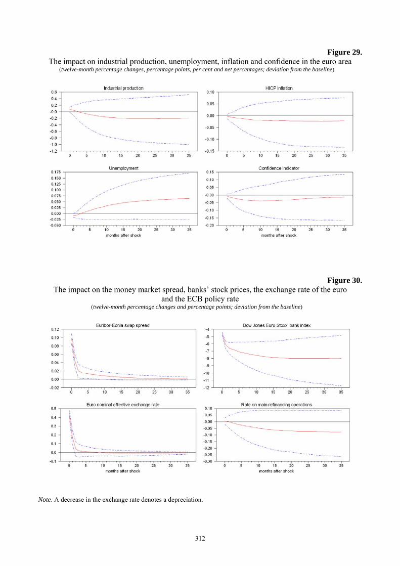
312
Figure 29.The impact on industrial production, unemployment, inflation and confidence in the euro area
(twelve-month percentage changes, percentage points, per cent and net percentages; deviation from the baseline)
Figure 30.The impact on the money market spread, banks’ stock prices, the exchange rate of the euro
and the ECB policy rate (twelve-month percentage changes and percentage points; deviation from the baseline)
Note. A decrease in the exchange rate denotes a depreciation.
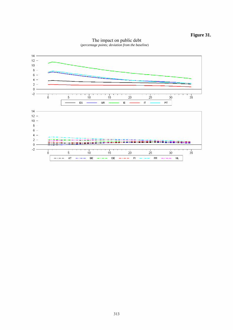
313
Figure 31.
The impact on public debt (percentage points; deviation from the baseline)
Recommended


