Download pdf - The Fast Lifting Wav elet Transform - Pusanharmony.cs.pusan.ac.kr/lecture/lecture_data/The Fast Lifting... · The Fast Lifting Wavelet Transform – © C. Valens, 1999 – [email protected]

The Fast Lifting WaveletTransform

© C. Valens, 1999

[email protected]

The Fast Lifting Wavelet Transform – © C. Valens, 1999 – [email protected]

2

Disclaimer

This tutorial is aimed at the engineer, not the mathematician. This does not mean that there will be nomathematics, it just means that there will be no proofs in the text. In my humble opinion, mathematicalpapers are completely unreadable because of the proofs that clutter the text. For proofs the reader ispointed to suitable references. The equations presented are there to illustrate and to clarify things, I hope.It should not be necessary to understand all the equations in order to understand the theory. However, tounderstand this tutorial, a mathematical background on an engineering level is required. Also someknowledge of signal processing theory might come in handy.

The information presented in this tutorial is believed to be correct. However, no responsibilty whatsoeverwill be accepted for any damage whatsoever due to errors or misleading statements or whatsoever in thistutorial. Should there be anything incorrect, incomplete or not clear in this text, please let me know so thatI can improve this tutorial.


3

Table of Contents

1. Introduction

2. Perfect reconstruction

3. The polyphase representation

4. Intermezzo: Laurent polynomials

5. Lifting

6. Factoring filters

7. Example

8. Lifting properties

9. Integer lifting

10. Coda

11. References


4

1. Introduction

This tutorial is a sequel to my wavelet tutorial, which will fill in the blank spots on the wavelet transform map, add

some detail and even explore the area outside it. We start with taking a closer look at the scaling and wavelet filters

in general, what they should look like, what their constraints are and how they can be used in the inverse wavelet

transform. Then we will do some algebra and develop a general framework to design filters for every possible

wavelet transform. This framework was introduced by Sweldens [Swe96a] and is known as the lifti ng scheme or

simply lif ting. Using the lifting scheme we will in the end arrive at a universal discrete wavelet transform which

yields only integer wavelet- and scaling coefficients instead of the usual floating point coeff icients. In order to clarify

the theory in this tutorial a detailed example will be presented.

In this tutorial we will go into some more detail compared to the wavelet transform tutorial, since the lifting scheme

is a quite recent development and especially integer lifting [Cal96], [Uyt97b] and multi-dimensional l ifting [Kov97],

[Uyt97a] are not (yet) widely known. This tutorial is mainly based on [Dau97], [Cal96], [Swe96a], [Swe96b],

[Cla97], [Uyt97b] and [Uyt97c].

Before we start a short note on notation. In order to be compatible with existing lifting literature I will use the same

symbols. This means that the analyzing filters are denoted as h~

and g~ , i.e. with a tilde, while the synthesizing filters

are denoted by a plain h and g. In fact, everything that has to do with the forward wavelet transform will carry a tilde.

I will however use a slightly different form here due to the fact that in [Dau97] the transposed version of )(~

zΡ is used

in all calculations and because the filters h~

and g~ are there defined as )(~ 1−zh and )(~ 1−zg instead of )(

~zh and )(~ zg .

In this tutorial λ stands for the scaling function coefficients and γ for the wavelet coefficients.

2. Perfect reconstruction

Usuall y a signal transform is used to transform a signal to a different domain, perform some operation on the

transformed signal and inverse transform it, back to the original domain. This means that the transform has to be

invertible. In case of no data processing we want the reconstruction to be perfect, i.e. we will allow only for a time

delay. All this holds also in our case of the wavelet transform.

As mentioned before, we can perform a wavelet transform (or subband coding or multi resolution analysis) using a

filter bank. A simple one-stage filter bank is shown in figure 1 and it can be made using FIR filters. Although IIR

filters can also be used, they have the disadvantage that their infinite response leads to infinite data expansion. For

any practical use of an IIR filter bank the output data stream has to be cut which leads to a loss of data. In this text

we will only look at FIR filters.


5

Figure 1

A one-stage filter bank for signal analysis and reconstruction.

Figure 1 shows how a one-stage wavelet transform uses two analysis filters, a low-pass filter h~

and a high-passfilter g~ followed by subsampling for the forward transform. From this figure it seems only logical to construct the

inverse transform by first performing an upsampling step and then to use two synthesis filters h (low-pass) and g

(high-pass) to reconstruct the signal. We need filters here, because the upsampling step is done by inserting a zero in

between every two samples and the filters will have to smooth this.

For the filter bank in figure 1 the conditions for perfect reconstruction are now given by [Dau97] as:

0

2

)(~)()(~

)(

)(~)()(~

)(11

11

==

−+−+

−−

−−

zgzgzhzh

zgzgzhzh . (1)

The time reversion of the analyzing filters is necessary to compensate for the delays in the filters. Without it, it

would be impossible to arrive at an non-delayed perfectly reconstructed signal. If the conditions for perfect

reconstruction are fulfill ed, then all the aliasing caused by the subsampling will miraculously be canceled during the

reconstruction.

3. The polyphase representation

In the filter stage shown in the left part of figure 1 the signal is first filtered and then subsampled. In other words, we

throw away half of the filtered samples and keep only the even-numbered samples, say. Clearly this is not efficient

and therefore we would like to do the subsampling before the filtering in order to save some computing time. Let us

take a closer look at what exactly is thrown away by subsampling.


6

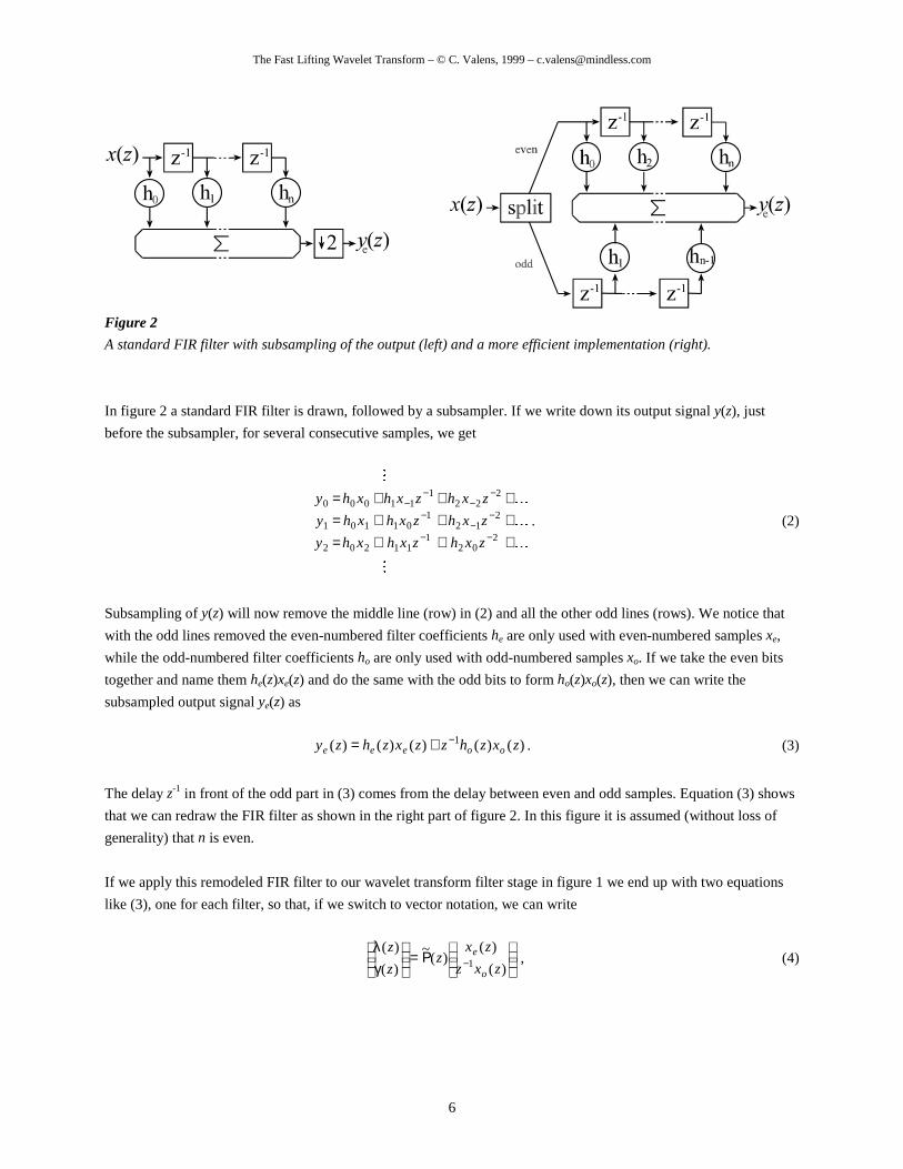
Figure 2

A standard FIR filter with subsampling of the output (left) and a more efficient implementation (right).

In figure 2 a standard FIR filter is drawn, followed by a subsampler. If we write down its output signal y(z), just

before the subsampler, for several consecutive samples, we get

�

�

�

�

+++

+++

+++

===

−

−−

−−

−

−

−−

202

212

222

111

101

111

20

10

00

2

1

0

zxh

zxh

zxh

zxh

zxh

zxh

xh

xh

xh

y

y

y

. (2)

�

Subsampling of y(z) will now remove the middle line (row) in (2) and all the other odd lines (rows). We notice that

with the odd lines removed the even-numbered filter coefficients he are only used with even-numbered samples xe,

while the odd-numbered filter coefficients ho are only used with odd-numbered samples xo. If we take the even bits

together and name them he(z)xe(z) and do the same with the odd bits to form ho(z)xo(z), then we can write the

subsampled output signal ye(z) as

)()()()()( 1 zxzhzzxzhzy ooeee−+= . (3)

The delay z-1 in front of the odd part in (3) comes from the delay between even and odd samples. Equation (3) shows

that we can redraw the FIR filter as shown in the right part of figure 2. In this figure it is assumed (without loss of

generality) that n is even.

If we apply this remodeled FIR filter to our wavelet transform filter stage in figure 1 we end up with two equations

like (3), one for each filter, so that, if we switch to vector notation, we can write

Ρ=

γλ

− )(

)()(

~)(

)(1 zxz

zxz

z

z

o

e , (4)


7

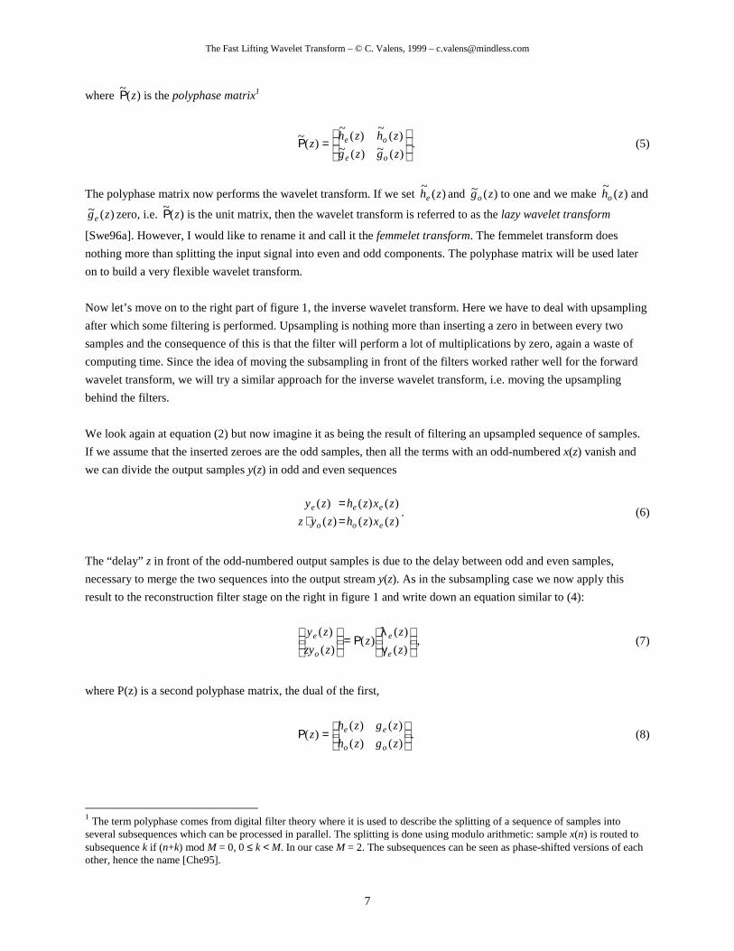
where )(~

zΡ is the polyphase matrix1

=Ρ

)(~)(~)(

~)(

~)(

~

zgzg

zhzhz

oe

oe . (5)

The polyphase matrix now performs the wavelet transform. If we set )(~

zhe and )(~ zgo to one and we make )(~

zho and

)(~ zge zero, i.e. )(~

zΡ is the unit matrix, then the wavelet transform is referred to as the lazy wavelet transform

[Swe96a]. However, I would like to rename it and call it the femmelet transform. The femmelet transform does

nothing more than spli tting the input signal into even and odd components. The polyphase matrix will be used later

on to build a very flexible wavelet transform.

Now let’s move on to the right part of figure 1, the inverse wavelet transform. Here we have to deal with upsampling

after which some filtering is performed. Upsampling is nothing more than inserting a zero in between every two

samples and the consequence of this is that the filter will perform a lot of multiplications by zero, again a waste of

computing time. Since the idea of moving the subsampling in front of the filters worked rather well for the forward

wavelet transform, we will t ry a similar approach for the inverse wavelet transform, i.e. moving the upsampling

behind the filters.

We look again at equation (2) but now imagine it as being the result of filtering an upsampled sequence of samples.

If we assume that the inserted zeroes are the odd samples, then all the terms with an odd-numbered x(z) vanish and

we can divide the output samples y(z) in odd and even sequences

)()(

)()(

)(

)(

zxzh

zxzh

zyz

zy

eo

ee

o

e

==

⋅. (6)

The “delay” z in front of the odd-numbered output samples is due to the delay between odd and even samples,

necessary to merge the two sequences into the output stream y(z). As in the subsampling case we now apply this

result to the reconstruction filter stage on the right in figure 1 and write down an equation similar to (4):

γλ

Ρ=

)(

)()(

)(

)(

z

zz

zzy

zy

e

e

o

e , (7)

where P(z) is a second polyphase matrix, the dual of the first,

=Ρ

)()(

)()()(

zgzh

zgzhz

oo

ee . (8)

1 The term polyphase comes from digital filter theory where it is used to describe the splitting of a sequence of samples intoseveral subsequences which can be processed in parallel. The splitti ng is done using modulo arithmetic: sample x(n) is routed tosubsequence k if (n+k) mod M = 0, 0 ≤ k < M. In our case M = 2. The subsequences can be seen as phase-shifted versions of eachother, hence the name [Che95].


8

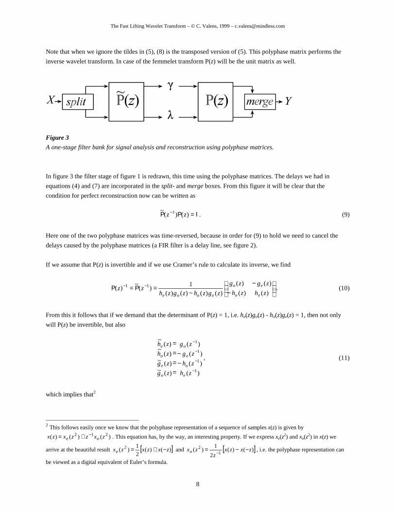
Note that when we ignore the tildes in (5), (8) is the transposed version of (5). This polyphase matrix performs the

inverse wavelet transform. In case of the femmelet transform P(z) will be the unit matrix as well .

Figure 3

A one-stage filter bank for signal analysis and reconstruction using polyphase matrices.

In figure 3 the filter stage of figure 1 is redrawn, this time using the polyphase matrices. The delays we had in

equations (4) and (7) are incorporated in the split - and merge boxes. From this figure it will be clear that the

condition for perfect reconstruction now can be written as

Ι=ΡΡ − )()(~ 1 zz . (9)

Here one of the two polyphase matrices was time-reversed, because in order for (9) to hold we need to cancel the

delays caused by the polyphase matrices (a FIR filter is a delay line, see figure 2).

If we assume that P(z) is invertible and if we use Cramer’s rule to calculate its inverse, we find

−

−−

=Ρ=Ρ −−

)()(

)()(

)()()()(

1)(

~)( 11

zhzh

zgzg

zgzhzgzhzz

eo

eo

eooe

. (10)

From this it follows that if we demand that the determinant of P(z) = 1, i.e. he(z)go(z) - ho(z)ge(z) = 1, then not only

will P(z) be invertible, but also

)(

)(

)(

)(

)(~)(~)(

~)(

~

1

1

1

1

−

−

−

−

−−

====

zh

zh

zg

zg

zg

zg

zh

zh

e

o

e

o

o

e

o

e

, (11)

which implies that2

2 This follows easily once we know that the polyphase representation of a sequence of samples x(z) is given by

)()()( 212 zxzzxzx oe−+= . This equation has, by the way, an interesting property. If we express xe(z

2) and xo(z2) in x(z) we

arrive at the beautiful result [ ])()(2

1)( 2 zxzxzxe −+= and [ ])()(

2

1)(

12 zxzx

zzxo −−=

−, i.e. the polyphase representation can

be viewed as a digital equivalent of Euler’s formula.


9

)(

)(

)(~)(

~

11

11

−−

−−

−−−

==

zhz

zgz

zg

zh. (12)

In the special case that h = h~

and g = g~ the wavelet transform is orthogonal, otherwise it is biorthogonal.

If the polyphase matrix has a determinant of 1, then the filter pair (h,g) is called complementary. If the filter pair

(h,g) is complementary, so is the filter pair ( h~

, g~ ).

Note that if the determinant of P(z) = 1 the filters he(z) and ho(z) have to be relatively prime and we will exploit this

property in the section on filter factoring. Of course the pairs ge(z) and go(z), he(z) and ge(z) and ho(z) and go(z) will

also be relatively prime.

Summarizing we can state that the problem of finding an invertible wavelet transform using FIR filters amounts to

finding a matrix P(z) with determinant 1. From this matrix the four filters needed in the invertible wavelet transform

follow immediately. Compare this to the definition of the continuous wavelet transform at the beginning of the

wavelet tutorial. We sure have come a long way! But there is more to come.

4. Intermezzo: Laurent polynomials

As an intermezzo some algebra will now be presented, which we will need in the following sections.

The z-transform of a FIR filter is given by

∑=

−=q

pk

kk zhzh )( . (13)

This summation is also known as a Laurent polynomial or Laurent series3. A Laurent polynomial differs from a

normal polynomial in that it can have negative exponents. The degree of a Laurent polynomial h is defined as

pqh −= , (14)

so that the length of the filter is equal to the degree of the associated polynomial plus one. Note that the Laurent

polynomial zp has degree zero. The sum or difference of two Laurent polynomials is again a Laurent polynomial and

the product of two Laurent polynomials of degree a and b is a Laurent polynomial of degree a+b. Exact division is in

general not possible, but division with remainder is. This means that for any two Laurent polynomials a(z) and b(z) ≠0, with |a(z)| ≥ |b(z)| there will always exist a Laurent polynomial q(z) with |q(z)| = |a(z)| - |b(z)|, and a Laurent

polynomial r(z) with |r(z)| < |b(z)| so that

)()()()( zrzqzbza += . (15)

3 Like the Taylor series, Laurent series can be used to expand functions in.


10

This division is not necessarily unique.

Finally we remark that a Laurent polynomial is invertible if and only if it is of degree zero, i.e. if it is a monomial.

In the following sections we will unleash the power of algebra on the polyphase matrices. The result will be an

extremely powerful algorithm to build wavelet transforms.

5. Lifting

As will be clear from our intermezzo the polyphase matrix is a matrix of Laurent polynomials and since we

demanded that its determinant be equal to 1, we know that the filter pair (h,g) is complementary. The lifti ng theorem

[Dau97] now states that any other finite filter gnew complementary to h is of the form

)()()()( 2zszhzgzgnew += , (16)

where s(z2) is a Laurent polynomial. This can be seen very easily if we write gnew in polyphase form (see also the

footnote with equation (12)) and assemble the new polyphase matrix as

Ρ=

++

=Ρ10

)(1)(

)()()()(

)()()()()(

zsz

zgzszhzh

zgzszhzhz

ooo

eeenew . (17)

As can be easily verified the determinant of the new polyphase matrix also equals 1, which proofs (16).

Similarly, we can apply the lifting theorem to create the filter )(~

zh new complementary to )(~ zg (recall the identities

from (11))

)(~)(~)(~

)(~ 2zszgzhzh new += , (18)

with the new dual polyphase matrix given by

)(~

10

)(~1

)(~)(~)(~)(~)(

~)(~)(~)(

~)(

~z

zs

zgzg

zszgzhzszgzhz

oe

ooeenew Ρ

=

++=Ρ . (19)

What we just did is called primal lifti ng, we lifted the low-pass subband with the help of the high-pass subband.

Figure 4 shows the effect of primal l ifting graphicall y.


11

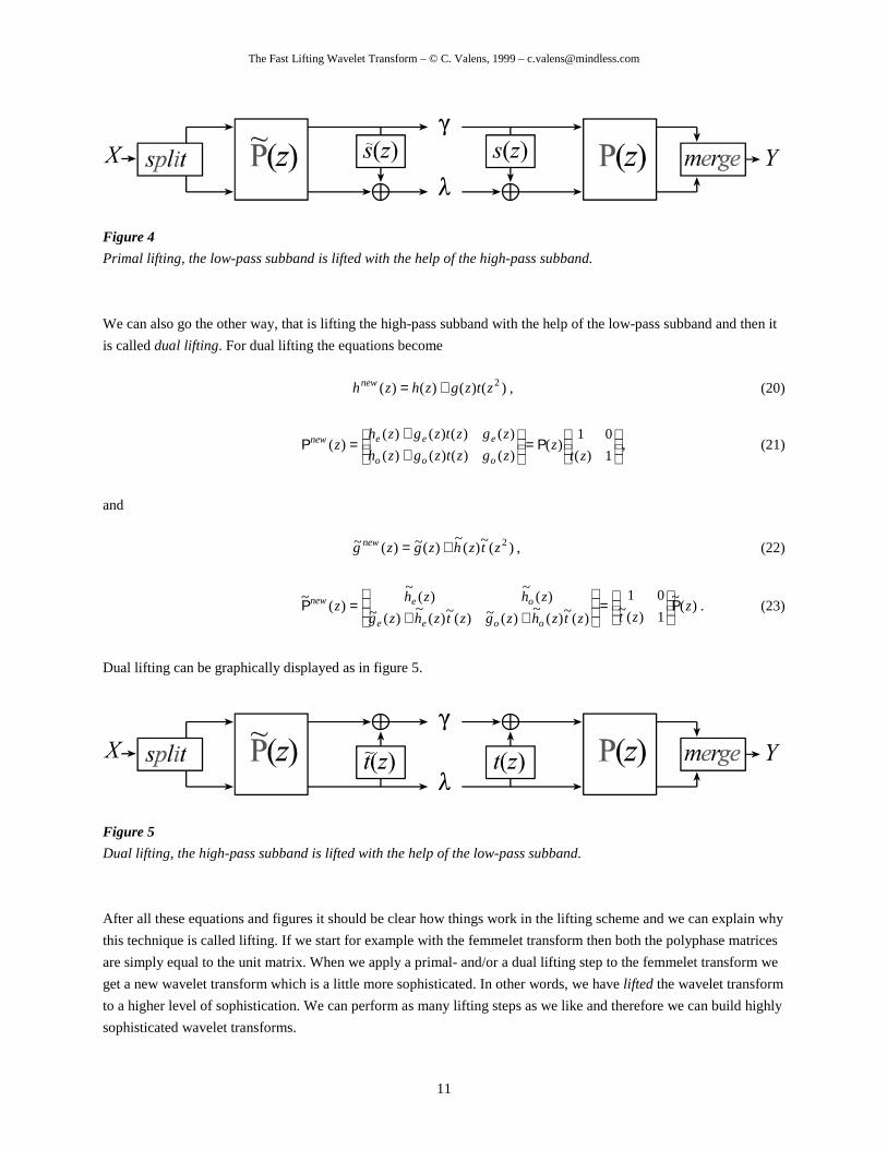
Figure 4

Primal lifti ng, the low-pass subband is lifted with the help of the high-pass subband.

We can also go the other way, that is lifting the high-pass subband with the help of the low-pass subband and then it

is called dual lifti ng. For dual li fting the equations become

)()()()( 2ztzgzhzhnew += , (20)

Ρ=

++

=Ρ1)(

01)(

)()()()(

)()()()()(

ztz

zgztzgzh

zgztzgzhz

ooo

eeenew , (21)

and

)(~)(~

)(~)(~ 2ztzhzgzgnew += , (22)

)(~

1)(~01

)(~)(~

)(~)(~)(~

)(~)(

~)(

~)(

~z

ztztzhzgztzhzg

zhzhz

ooee

oenew Ρ

=

++=Ρ . (23)

Dual l ifting can be graphicall y displayed as in figure 5.

Figure 5

Dual lifti ng, the high-pass subband is lifted with the help of the low-pass subband.

After all these equations and figures it should be clear how things work in the li fting scheme and we can explain why

this technique is called li fting. If we start for example with the femmelet transform then both the polyphase matrices

are simply equal to the unit matrix. When we apply a primal- and/or a dual li fting step to the femmelet transform we

get a new wavelet transform which is a littl e more sophisticated. In other words, we have lifted the wavelet transform

to a higher level of sophistication. We can perform as many li fting steps as we like and therefore we can build highly

sophisticated wavelet transforms.


12

The inverse lifting transform now also begins to take shape. If we start with a femmelet transform we only split the

input stream into an even and an odd stream. Then we lift one of these streams as in the left of figures 4 and 5 by

applying a Laurent polynomial to the other and adding it to the first. We can very easily undo this lifting step by

again applying the same Laurent polynomial to the other stream and then subtract it from the first. In other words,

inverting a lifting transform is the same as changing all the signs of the lifting Laurent polynomials in figures 4 and 5

and run it backwards, i.e. start at the output. Inverting the lifting scheme this way will always work! From this wecan conclude that )(~)( ztzt −= and )(~)( zszs −= .

From the figures 4 and 5 we can see another interesting property of lifting. Every time we apply a primal or dual

li fting step we add something to one stream. All the samples in the stream are replaced by new samples and at any

time we need only the current streams to update sample values. In other words, the whole transform can be done in-

place, without the need for auxiliary memory. This is the same as with the fast Fourier transform, where the

transformed data also takes the same place as the input data. This in-place property makes the lifting wavelet

transform very attractive for use in embedded applications, where memory and board space are still expensive.

We conclude this section with a note on terminology. In lifting literature the dual l ifting step is also referred to as the

predict step, while the primal l ifting step is also referred to as the update step. The idea behind this terminology is

that lifting of the high-pass subband with the low-pass subband can be seen as prediction of the odd samples from the

even samples. One assumes that, especially at the first steps, consecutive samples will be highly correlated so that it

should be possible to predict the odd ones from the even ones (or the other way around). The update step, i.e. li fting

the low-pass subband with the high-pass subband, then is done to keep some statistical properties of the input stream,

usually at least the average, of the low-pass subband.

6. Factoring filters

In the previous section we lifted a wavelet transform to a more sophisticated level. Of course we can also do the

opposite, i.e. we can factor the FIR filters of an existing wavelet transform into lifting steps. This would be very

useful because a lot of research has already been performed on designing wavelet filters for all kinds of applications

and factoring these filters will allow us to benefit easily from this research. So how do we go about?

Starting with for instance equation (22) we can go the other way by writing

)(~)(~)(~

)(~ 2 zgztzhzg new+= . (24)

The form of (24) is identical to a long division with remainder of Laurent polynomials, where )(~ zgnew is the

remainder. If we rewrite equation (23) a littl e as well , we obtain

)(~

1)(~01

)(~)()(~

)(~)()(~

)(~

)(~

)(~

zztzgztzhzgztzh

zhzhz new

newoo

newee

oe Ρ

=

++=Ρ , (25)


13

and we see that for the polyphase matrix we have to perform two long divisions in order to extract one li fting step.

Once we have extracted one such lifting step we can continue by extracting more lifting steps from the new

polyphase matrix until we end up with the unit matrix, or a matrix with only two constants on its main diagonal. In

fact, in [Dau97] it is proven that it will always be possible to do this when we start with a complementary filter pair

(h,g), i.e. P(z) can always be factored into lifting steps:

∏=

î

=Ρ

m

i i

i

zt

zs

K

Kz

12

1

1)(

01

10

)(1

0

0)( . (26)

In equation (26) K1 and K2 are scaling constants unequal to zero. If scaling is not desired for some reason, it is even

possible to factor the scaling matrix into four more lifting steps, one of which can be combined with the last real

li fting step so that factoring a scaling matrix costs three extra li fting steps [Dau97].

To perform a long division with remainder on Laurent polynomials we can use the Euclidean algorithm for Laurent

polynomials4. The Euclidean algorithm was originally developed to find the greatest common divisor (gcd) of two

natural numbers, but we can extend it to Laurent polynomials as well . In [Dau97] it is given as:

Take two Laurent polynomials a(z) and b(z) ≠ 0 with |a(z)| ≥ |b(z)|. Let a0(z) =

a(z) and b0(z) = b(z) and iterate the following steps starting from i = 0

)(/)()(

)()%()(

)()(

1

1

1

zbzazq

zbzazb

zbza

iii

iii

ii

===

+

+

+

(27)

Then an(z) = gcd(a(z),b(z)) where n is the smallest number for which bn(z) = 0.

The ‘%’-symbol in the second line of (27) means mod, i.e. integer divide with remainder but only keeping the

remainder, and it is the same symbol as used in the C programming language for the mod operation. The ‘ /’ -symbol

in the third line is the C-language div operator. The result of this algorithm can be written as

∏=

=

n

i

ni zazq

zb

za

10

)(

01

1)(

)(

)(, (28)

which looks very much like a series of lifting steps. The gcd found might not be unique since it is defined only up to

a factor zp, i.e. there are several factorizations possible. This turns out to be an advantage because it allows us to

select the factoring which best suits our needs.

4 Why? We write the long division with remainder of a0 and a1 as a0 = q1·a1 + a2. But we can express a1 in a similar way as a1 =q2·a2 + a3 and a2 also, and so on. The row of remainders will eventually reach zero, a1> a2>…> an> an+1= 0, and this is where itstops. The gcd of a0 and a1 is now an. However, we are more interested in the intermediate results a0 = q1·( q2·(…( qn·an + an+1)+…) + a3) + a2 (remember an+1 = 0) or written as in (28) [Coh95].


14

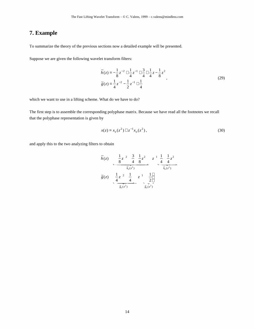
7. Example

To summarize the theory of the previous sections now a detailed example will be presented.

Suppose we are given the following wavelet transform filters:

4

1

2

1

4

1)(~

8

1

4

1

4

3

4

1

8

1)(

~

12

212

+−=

−+++−=

−−

−−

zzzg

zzzzzh, (29)

which we want to use in a li fting scheme. What do we have to do?

The first step is to assemble the corresponding polyphase matrix. Because we have read all the footnotes we recall

that the polyphase representation is given by

)()()( 212 zxzzxzx oe−+= , (30)

and apply this to the two analyzing filters to obtain

��

� ��

)(~

1

)(~

2

)(~

21

)(~

22

22

22

2

1

4

1

4

1)(~

4

1

4

1

8

1

4

3

8

1)(

~

zgzg

zhzh

oe

oe

zzzg

zzzzzh

î −+

î +=

î ++

î −+−=

−−

−−

, (31)

which means that

2

1)(~

4

1

4

1)(~

4

1

4

1)(

~

8

1

4

3

8

1)(

~

1

1

−=+=

+=−+−=

−

−

zgzzg

zzhzzzh

oe

oe, (32)

and thus

−+

+−+−=Ρ

−

−

2

1

4

1

4

14

1

4

1

8

1

4

3

8

1

)(~

1

1

z

zzzz . (33)

With the help of (11) we can now assemble the synthesizing polyphase matrix as well. First we check the

determinant of (33):

2

1

4

1

4

1

4

1

4

1

2

1

8

1

4

3

8

1 11 −=

+

+−

−

−+− −− zzzz , (34)

so we have to scale (11) a bit before using the equaliti es to get:


15

+−+

+=Ρ

−

−

zzz

zz

4

1

2

3

4

1

2

1

2

12

1

2

11

)(1

1

. (35)

Do not get confused here, P(z) is not time-reversed! Remember, if we want to check (9) we have to time-reverse one

of the polyphase matrices. From (35) we can find the synthesizing filters as follows:

zzzgzzg

zzhzh

oe

oe

4

1

2

3

4

1)(

2

1

2

1)(

2

1

2

1)(1)(

11 +−=+=

+==

−−, (36)

thus

{ }

��

� ��

)(

221

)(

2

)(

21

)(

22

2

2

4

1

2

3

4

1

2

1

2

1)(

2

1

2

11)(

zgzg

zhzh

oe

o

e

zzzzzg

zzzh

î +−+

î +=

î ++=

−−−

−

, (37)

so that

zzzzzg

zzzh

4

1

2

1

2

3

2

1

4

1)(

2

11

2

1)(

123

1

++−+=

++=

−−−

−

. (38)

Note that it is not necessary to actually calculate the synthesizing filters because of the simple reversibili ty of the

forward transform. We have done it here just to ill ustrate how things work.

The next step is the factoring of the polyphase matrices into lifting steps. We start with the extraction of a dual l ifting

step5.

−

+=Ρ

1)(~01

2

1)(~

4

1

4

1)(

~

)(~

ztzg

zzhz

newe

newe

, (39)

which means that we have to solve the following two equations:

)(~2

1)(~

4

1

4

1

)(~

4

1

4

1)(~

8

1

4

3

8

1

1

1

zgztz

zhzztzz

newe

newe

+

−=+

+

+=−+−

−

−

. (40)

5 Why? Because )(

~zh is the longest filter.


16

We use the Euclidean algorithm with a0 = )(~

zhe and b0 = )(~

zho and perform one step. Now note that there are three

possibiliti es for q1, and thus for b1, depending on which two terms of a0 you want to match with b0:

î

−

+

−

+

+

−−

−

+

+−

=−+−

−−

−

−

−

11

1

1

1

4

1

4

1

2

1

2

7

14

1

4

1

2

1

2

14

1

4

1

2

7

2

1

8

1

4

3

8

1

zzz

zz

zzz

zz . (41)

Note also that we have found three greatest common divisors. If we choose the middle line of (41) as thefactorization we have a symmetrical one, which goes nicely with )(~ zg as well , and we arrive at the following

decomposition:

−

−

+=Ρ − 1

2

1

2

101

2

10

4

1

4

11

)(~

1z

zz . (42)

We can continue by extracting a primal l ifting step. For this we apply the Euclidean algorithm to )(~ zge and )(~ zgo of

(42), almost not worth mentioning it, and find:

−

+

−=Ρ − 1

2

1

2

101

104

1

4

11

2

10

01)(

~1z

zz . (43)

This equation gives a fully factored version of the filters from (29). If we finally use (43) with (4) we can display our

wavelet transform graphically as in figure 6 while the corresponding wavelet and scaling function are displayed in

figure 7.

Figure 6

The implementation of the wavelet transform of this example.


17

From figure 6 we can generalize the lifting steps as:

)()(~)()(

)()(~)()(

zzszz

zztzznew

new

γ+λ=λ

λ+γ=γ, (44)

to emphasize the in-place calculation property of the lifting transform.

Figure 7

The scaling function (left) and the wavelet (right) that go with this example.

8. Lifting properties

The li fting scheme has some properties which are not found in many other transforms. Figure 6 shows a few of these

properties and we will now take a look at some of the most important ones.

The inverse transform is immediately clear: change the signs of all the scaling factors, replace “split ” by “merge” and

go from right to left, i.e. reverse the data flow. This easy invertibili ty is always true for the li fting scheme.

Lifting can be done in-place (see 42): we never need samples other than the output of the previous li fting step and

therefore we can replace the old stream by the new stream at every summation point. Not immediately clear from

this figure is that when we iterate a filter bank using in-place lifted filters we end up with interlaced coefficients. This

can be seen as follows. We split the input in odd- and even-numbered samples and perform the in-place lifting steps.

After one complete step the high-pass filtered samples, the wavelet coefficients, sit in the odd-numbered places and

the low-pass filtered samples sit in the even-numbered places. Then we perform another transform step, but only

using the low-pass filtered samples, so that this sequence will again be divided into odd- and even-numbered

samples. Again the odd-numbered samples are transformed into wavelet coefficients, while the even-numbered

samples will be processed further so that in the end all wavelet coefficients will be interlaced.


18

The third important property has not been mentioned yet, but it shows clearly from figure 6: li fting is not causal.

Usuall y this is not really a problem, we can always delay the signal enough to make it causal, but it will never be

real-time. In some cases however it is possible to design a causal li fting transform.

The last important property I will mention here is the calculation complexity. In [Dau97] it is proven that for long

filters the lifting scheme cuts computation complexity in half, compared to the standard iterated FIR filter bank

algorithm. This type of wavelet transform has already a complexity of N, in other words, much more efficient than

the FFT with its complexity of Nlog(N) and lifting speeds things up with another factor of two. This is where the title

of this tutorial comes from: it is a fast wavelet transform and therefore we will refer to it as the fast lifti ng wavelet

transform of FLWT.

9. Integer lifting

The last stage of our voyage to the ultimate6 wavelet transform is the stage where we make sure that the wavelet

coeff icients are integers. In classical transforms, including the non-lifted wavelet transforms, the wavelet coefficients

are assumed to be floating point numbers. This is due to the filter coeff icients used in the transform filters, which are

usually floating point numbers. In the li fting scheme it is however rather easy to maintain integer data, although the

dynamic range of the data might increase. That this is possible in the lifting scheme has to do with the easy

invertibili ty property of lifting.

The basic li fting step is given in (44) and we rewrite it here a littl e modified as [Uyt97]:

)()()()( zyzszxzxnew +← . (45)

Because the signal part y(z) is not changed by the lifting step, the result of the filter operation can be rounded, and we

can write:

)()()()( zyzszxzxnew +← , (46)

where we have used ⋅ to denote the rounding operation. Equation (46) is fully reversible:

)()()()( zyzszxzx new −← , (47)

and this shows the most amazing feature of integer lifting: whatever rounding operation is used, the lifting operation

will always be reversible.

We have to take care however, because we did not consider the scaling step in the previous paragraph. Scaling

usually does not yield integer results but it is a part of the lifting transform. The simplest solution to this problem is

to forget all about scaling and just keep in mind that the transform coeff icients actually have to be scaled. This is

important for instance in denoising applications. If scaling is ignored, then it is desirable to let the scaling factor be

6 That is, in our limited world, i.e. the context of this tutorial.


19

as close to one as possible. This can be done using the non-uniqueness of the lifting factorization. Another solution is

to factor the scaling into lifting steps as well [Dau97].

As mentioned before the integer lifting transform can not guarantee the preservation of the dynamic range of the

input signal. Usually the dynamic range doubles [Uyt97c], but there are schemes that can keep the dynamic range. In

[Cha96] an interesting lifting transform with the so-called property of precision preservation (PPP) is described.

This transform makes use of the two-complement representation of integers in a computer and the wrap-around

overflows cause in this representation. The disadvantage of such a transform is that large coefficients may be

represented by small values and it is therefore difficult to take decisions on coefficient values.

10. Coda

We have now finished our self-imposed task of transforming the CWT into a practical implementation. In this

tutorial we have seen how we can use the lifting scheme to build a very versatile wavelet transform. After first

optimizing the subsampled and upsampled FIR filters from the wavelet tutorial, through the use of some algebra we

arrived at a scheme to build a wavelet transform using primal and dual l ifting blocks. These modules allowed us to

build any wavelet transform, which fits in the classical framework, and more. Adapting the lifting scheme we will be

well armed: amongst our weaponry are such elements as7 easy invertibili ty of any transform, in-place calculation of

the transform and easy integer transform coefficients without losing any of its features. And there are many more

features [Cal96], [Uyt97b], [Dau97].

However, this does not mean that this is the only way to go. There are probably as many wavelet transforms as there

are wavelets. Due to the infinite variety of wavelets it is possible to design a transform which maximally exploits the

properties of a specific wavelet8, and of course this has been done. While researching wavelet theory I stumbled

upon morlets9, coiflets, wavelants, slantlets, brushlets and wavelet packets to name a few. The li fting scheme on the

other hand is a really general scheme, which makes it very suitable for experimenting while the in-place and integer

properties make it extremely useful for embedded systems where memory is still expensive. With the application

described in this report in mind, it will be clear that these are the reasons for studying the lifting scheme.

Finally, four remarks to conclude this tutorial:

• In [Uyt97b] the filter factoring algorithm is used to split the original filters in simpler filters and one primal and

dual li fting step. These lifting steps are then used to make the original wavelet transform integer. This is some

kind of hybrid (trans)form but very effective.

• Up to now we have only spoken about one-dimensional transforms. It is however easily possible to extend the

li fting transform to the multi-dimensional case. Not only can the lifting transform be used in a classical 7 “Our chief weapon is surprise … surprise and fear… fear and surprise … Our two weapons are fear and surprise … andruthless efficiency … Our three weapons are fear, surprise, and ruthless efficiency … and an almost fanatical devotion to thePope … Our four … no … Amongst our weapons … Amongst our weaponry … are such elements as fear, surprise …” FromMonthy Python’s Flying Circus, series 2, episode 15, “The Spanish Inquisition” (1970).8 Compare this to the Fourier transform, where a sine will always be a sine.9 Very funny indeed, Morlet [Mor82] being more or less the inventer of wavelets, but used as such in [Wei94].


20

separable multi-dimensional setting, but it can be made truly multi-dimensional. In [Uyt97a] the lifting

transform is extended to a true two-dimensional transform, while in [Kov97] the complete theoretical

foundations are laid out for any dimension. The principles behind lifting do not change at all i n the multi-

dimensional setting.

• One of the advantages of the li fting scheme as pointed out in for instance [Dau97] and [Cal96] is that the lifting

scheme allows for an introduction into wavelet theory without the use of Fourier theory. I do not agree with this

on the grounds that from the li fting scheme it is totall y unclear why there should be wavelets in it at all . The

concept of wavelets is completely unnecessary to understand the lifting scheme and therefore, I feel, it should

not be used as an introduction to wavelet theory.

• The li fting scheme is constantly under development and is investigated by many. Recent additions are the li fting

scheme in a redundant setting in order to improve the translation invariance [Sto98] and adaptive prediction

schemes for integer li fting [Cla97].

11. References

Books and papers

[Cal96] Calderbank, A. R. and I. Daubechies, W. Sweldens, B.-L. YeoWAVELET TRANSFORMS THAT MAP INTEGERS TO INTEGERS.Proceedings of the IEEE Conference on Image Processing. Preprint, 1996.IEEE Press, 1997. To appear.

[Che95] Chen, W.-K., editor.THE CIRCUITS AND FILTERS HANDBOOK.Boca Raton, Fl (USA): CRC Press, 1995.The Electrical Engineering Handbook Series.

[Cla97] Claypoole, R. and G. Davis, W. Sweldens, R. Baraniuk.NONLINEAR WAVELET TRANSFORMS FOR IMAGE CODING.Asilomar Conference on Signals, Systems, and Computers. Preprint, 1997.To appear.

[Dau97] Daubechies, I. and W. Sweldens.FACTORING WAVELET TRANSFORMS INTO LIFTING STEPS.J. Fourier Anal. Appl., Vol. 4, Nr. 3, 1998, preprint.

[Kov97] Kovacevic, J. and W. SweldensWAVELET FAMILIES OF INCREASING ORDER IN ARBITRARY DIMENSIONS.To appear in IEEE Transactions on Image Processing. Preprint 1997.

[Mor82] Morlet, J. and G. Arens, I. Fourgeau, D. Giard.WAVE PROPAGATION AND SAMPLING THEORY.Geophysics, Vol. 47 (1982), p. 203-236.

[Sto98] Stoffel, A.


21

REMARKS ON THE UNSUBSAMPLED WAVELET TRANSFORM AND THE LIFTINGSCHEME.Elsevier Science. Preprint, 1998.

[Swe96a] Sweldens, W.THE LIFTING SCHEME: A CONSTRUCTION OF SECOND GENERATION WAVELETS.Siam J. Math. Anal, Vol. 29, No. 2 (1997). Preprint, 1996.

[Swe96b] Sweldens, W.BUILDING YOUR OWN WAVELETS AT HOME.In: Wavelets in Computer Graphics.ACM SIGGRAPH Course Notes, 1996.

[Uyt97a] Uytterhoeven G. and A. Bultheel.THE RED-BLACK WAVELET TRANSFORM.Technical report TW271, Department of Computer Science.Leuven: Katholieke Universiteit Leuven, 1997.

[Uyt97b] Uytterhoeven G. and F. Van Wulpen, M. Jansen, D. Roose, A. Bultheel.WAILI: WAVELETS WITH INTEGER LIFTING.Technical report TW262, Department of Computer Science.Leuven: Katholieke Universiteit Leuven, 1997.

[Uyt97c] Uytterhoeven G. and D. Roose, A. Bultheel.WAVELET TRANSFORMS USING THE LIFTING SCHEME.Report ITA-Wavelets-WP1.1, Department of Computer Science.Leuven: Katholieke Universiteit Leuven, 1997.

[Wei94] Weiss, L. G.WAVELETS AND WIDEBAND CORRELATION PROCESSING.IEEE Signal Processing Magazine, January (1994), p. 13-32.

Internet resources

Besides classical references there are many Internet sources that deal with wavelets. Here I have listed a few thathave proved to be useful. With these links probably every other wavelet related site can be found. Keep in mindhowever that this list was compiled in July 1999.

• The Wavelet Digest, a monthly electronic magazine currently edited by Wim Sweldens [Swe96a,b], is a platformfor people working with wavelets. It contains announcements of conferences, abstracts of publications andpreprints and questions and answers of readers. It can be found at www.wavelet.org/wavelet/index.html and it isthe site for wavelets.

• MathsoftÒ , the makers of MathcadÒ , maintain a wavelet site called wavelet resources, which contains a hugelist of wavelet-related papers and links. It is located at www.mathsoft.com/wavelets.html

• Rice University, the home of Burrus [Bur98] et al, keeps a list of publications and makes available the RiceWavelet Toolbox for MatLabÒ at www-dsp.rice.edu/publications/

• The Katholieke Universiteit of Leuven, Belgium, is active on the net with wavelets, publications and the toolboxWAILI, at www.cs.kuleuven.ac.be/~wavelets/

• Amara Graps maintains a long list of links, publications and tools besides explaining wavelet theory in a nutshellat www.amara.com/current/wavelet.html


22

• There is a real li fting page, dedicated to Liftpack, a li fting toolbox atwww.cs.sc.edu/~fernande/liftpack/index.html

• Finally I would like to mention an interesting tutorial aimed at engineers by Robi Polikar from Iowa StateUniversity at www.public.iastate.edu/~rpolikar/WAVELETS/