Download pdf - The Direct Stiffness Method - SDC · PDF fileThe Direct Stiffness Method 2-3 2.2 One-dimensional Truss Element The simplest type of engineering structure is the truss structure. A

Introduction to Finite Element Analysis 2-1

Chapter 2 The Direct Stiffness Method

♦ Understand system equations for truss elements.

♦ Understand the setup of a Stiffness Matrix.

♦ Apply the Direct Stiffness Method. ♦ Create an Extruded solid model using

I-DEAS. ♦ Use the Display Viewing commands. ♦ Use the Sketch in Place command. ♦ Create Cutout features. ♦ Use the Basic Modify commands.

2-2 Introduction to Finite Element Analysis

2.1 Introduction The direct stiffness method is used mostly for Linear Static analysis. The development of the direct stiffness method originated in the 1940s and is generally considered the fundamental of finite element analysis. Linear Static analysis is appropriate if deflections are small and vary only slowly. Linear Static analysis omits time as a variable. It also excludes plastic action and deflections that change the way loads are applied. The direct stiffness method for Linear Static analysis follows the laws of Statics and the laws of Strength of Materials.

Stress-Strain diagram of typical ductile material This chapter introduces the fundamentals of finite element analysis by illustrating an analysis of a one-dimensional truss system using the direct stiffness method. The main objective of this chapter is to present the classical procedure common to the implementation of structural analysis. The direct stiffness method utilizes matrices and matrix algebra to organize and solve the governing system equations. Matrices, which are ordered arrays of numbers that are subjected to specific rules, can be used to assist the solution process in a compact and elegant manner. Of course, only a limited discussion of the direct stiffness method is given here, but we hope that the focused practical treatment will provide a strong basis for understanding the procedure to perform finite element analysis with I-DEAS. The later sections of this chapter demonstrate the procedure to create a solid model using I-DEAS Master Modeler. The step-by-step tutorial introduces the I-DEAS user interface and serves as a preview to some of the basic modeling techniques demonstrated in the later chapters.

Elastic Plastic STRAIN

STRESS

Linear Elastic region

Yield Point

The Direct Stiffness Method 2-3

2.2 One-dimensional Truss Element The simplest type of engineering structure is the truss structure. A truss member is a slender (the length is much larger than the cross section dimensions) two-force member. Members are joined by pins and only have the capability to support tensile or compressive loads axially along the length. Consider a uniform slender prismatic bar (shown below) of length L, cross-sectional area A, and elastic modulus E. The ends of the bar are identified as nodes. The nodes are the points of attachment to other elements. The nodes are also the points for which displacements are calculated. The truss element is a two-force member element; forces are applied to the nodes only, and the displacements of all nodes are confined to the axes of elements. In this initial discussion of the truss element, we will consider the motion of the element to be restricted to the horizontal axis (one-dimensional). Forces are applied along the X-axis and displacements of all nodes will be along the X-axis. For the analysis, we will establish the following sign conventions:

1. Forces and displacements are defined as positive when they are acting in the positive X direction as shown in the above figure.

2. The position of a node in the undeformed condition is the finite element

position for that node. If equal and opposite forces of magnitude F are applied to the end nodes, from the elementary strength of materials, the member will undergo a change in length according to the equation:

δ =

This equation can also be written as δ = F/K, which is similar to Hooke′s Law used in a linear spring. In a linear spring, the symbol K is called the spring constant or stiffness of the spring. For a truss element, we can see that an equivalent spring element can be used to simplify the representation of the model, where the spring constant is calculated as K=EA/L.

L

FF

A

+ X

FL EA


Force-Displacement Curve of a Linear Spring

We will use the general equations of a single one-dimensional truss element to illustrate the formulation of the stiffness matrix method:

By using the Relative Motion Analysis method, we can derive the general expressions of the applied forces (F1 and F2) in terms of the displacements of the nodes (X1 and X2) and the stiffness constant (K).

1. Let X1 = 0,

Based on Hooke’s law and equilibrium equation:

F2 = K X2 F1 = - F2 = - K X2

Force

Displacement

F

δK = EA/L

F

K

F1 F2

Node 1 Node 2

+X1 +X2

K = EA/L

F1 F2

Node 1 Node 2

X1= 0 +X2

K = EA/L


2. Let X2 = 0,

Based on Hooke’s Law and equilibrium:

F1 = K X1 F2 = - F1 = - K X1 Using the Method of Superposition, the two sets of equations can be combined:

F1 = K X1 - K X2 F2 = - K X1+ K X2 The two equations can be put into matrix form as follows:

F1 + K - K X1 F2 - K + K X2 This is the general force-displacement relation for a two-force member element, and the equations can be applied to all members in an assemblage of elements. The following example illustrates a system with three elements. Example 2.1: Consider an assemblage of three of these two-force member elements. (Motion is restricted to one-dimension, along the X-axis.)

F1 F2

Node 1 Node 2

X2= 0 +X1

K = EA/L

=

F K1

K2

K3 +X

Element 1

Element 2

Element 3


The assemblage consists of three elements and four nodes. The Free Body Diagram of the system with node numbers and element numbers labeled:

Consider now the application of the general force-displacement relation equations to the assemblage of the elements.

Element 1:

F1 + K1 - K1 X1 F21 - K1 + K1 X2

Element 2:

F22 + K2 - K2 X2 F3 - K2 + K2 X3

Element 3:

F23 + K3 - K3 X2 F4 - K3 + K3 X4

Expanding the general force-displacement relation equations into an Overall Global Matrix (containing all nodal displacements):

Element 1:

F1 + K1 - K1 0 0 X1

F21 - K1 + K1 0 0 X2 0 0 0 0 0 X3

0 0 0 0 0 X4

=

=

Element 3

F1

K1

K2

K3

Node 1 Node 2

Node 3

Node 4 +X1

+X2

+X3

+X4

F3

F4 Element 1

Element 2

=

=


Element 2:

0 0 0 0 0 X1 F22 0 +K2 -K2 0 X2

F3 0 -K2 +K2 0 X3 0 0 0 0 0 X4

Element 3:

0 0 0 0 0 X1 F23 0 +K3 0 -K3 X2

0 0 0 0 0 X3 F4 0 -K3 0 +K3 X4

Summing the three sets of general equation: (Note F2=F21+F22+F32)

F1 K1 -K1 0 0 X1 F2 -K1 (K1+K2+K3) -K2 -K3 X2

F3 0 -K2 K2 0 X3 F4 0 -K3 0 +K3 X4

Once the Overall Global Stiffness Matrix is developed for the structure, the next step is to substitute boundary conditions and solve for the unknown displacements. At every node in the structure, either the externally applied load or the nodal displacement is needed as a boundary condition. We will demonstrate this procedure with the following example.

Example 2.2: Given:

Find: Nodal displacements and reaction forces.

=

=

=

Overall Global Stiffness Matrix

F = 40 lbs.

K1= 50 lb/in

K3 = 70 lb/in +X

Element 1

Element 2

Element 3

Node 1 Node 2

Node 3

Node 4

K2 = 30 lb/in


Solution:

From example 2.1, the overall global force-displacement equation set:

F1 50 -50 0 0 X1 F2 -50 (50+30+70) -30 -70 X2

F3 0 -30 30 0 X3 F4 0 -70 0 70 X4

Next, apply the known boundary conditions to the system: the right-ends of element 2 and element 3 are attached to the vertical wall; therefore, these two nodal displacements (X3 and X4) are zero.

F1 50 -50 0 0 X1

F2 -50 (50+30+70) -30 -70 X2 F3 0 -30 30 0 0

F4 0 -70 0 70 0

The two displacements we need to solve the system are X1 and X2. Remove any unnecessary columns in the matrix:

F1 50 -50

F2 -50 150 X1 F3 0 -30 X2 F4 0 -70 Next, include the applied loads into the equations. The external load at Node 1 is 40 lbs. and there is no external load at Node 2.

40 50 -50

0 -50 150 X1 F3 0 -30 X2 F4 0 -70

The Matrix represents the following four simultaneous system equations:

40 = 50 X1 – 50 X2

0 = - 50 X1 + 150 X2 F3 = 0 X1 – 30 X2

F4 = 0 X1 – 70 X2

=

=

=

=


From the first two equations, we can solve for X1 and X2: X1 = 1.2 in. X2 = 0.4 in.

Substituting these known values into the last two equations, we can now solve for F3 and F4:

F3 = 0 X1 – 30 X2 = -30 x 0.4 = 12 lbs. F4 = 0 X1 – 70 X2 = -70 x 0.4 = 28 lbs.

From the above analysis, we can now reconstruct the Free Body Diagram (FBD) of the system:

The above sections illustrated the fundamental operation of the direct stiffness

method, the classical finite element analysis procedure. As can be seen, the formulation of the global force-displacement relation equations is based on the general force-displacement equations of a single one-dimensional truss element. The two-force-member element (truss element) is the simplest type of element used in FEA. The procedure to formulate and solve the global force-displacement equations is straightforward, but somewhat tedious. In real-life applications, the use of a truss element in one-dimensional space is rare and very limited. In the next chapter, we will expand the procedure to solve two-dimensional truss frameworks.

The following sections illustrate the procedure to create a solid model using I-DEAS Master Modeler. The step-by-step tutorial introduces the basic I-DEAS user interface and the tutorial serves as a preview to some of the basic modeling techniques demonstrated in the later chapters.

F1= 40 lbs. K1 K2

K3 1.2 in.

0.4 in. F3 = -12 lbs.

F4= -28 lbs.


2.3 Basic Solid Modeling using I-DEAS Master Modeler

One of the methods to create solid models in I-DEAS Master Modeler is to create a two-dimensional shape and then extrude the two dimensional shape to define a volume in the third dimension. This is an effective way to construct three-dimensional solid models since many designs are in fact the same shape in one direction. Computer input and output devices used today are largely two-dimensional in nature, which makes this modeling technique quite practical. This method also conforms to the design process that helps the designer with conceptual design along with the capability to capture the design intent. I-DEAS Master Modeler provides many powerful modeling tools and there are many different approaches available to accomplish modeling tasks. We will start by introducing the basic two-dimensional sketching and parametric modeling tools. The Adjuster Block design

Starting I-DEAS

1. Select the I-DEAS icon or type “ideas” at your system prompt to start I-DEAS. The I-DEAS Start window will appear on the screen.

2. Fill in and select the items as shown below:

Project Name: (Your account name) Model File Name: Adjuster Application: Design Task: Master Modeler


3. After you click OK, two warning

windows will appear to tell you that a new model file will be created. Click OK on both windows as they come up.

I-DEAS Warning ! New Model File will be created OK

4. Next, I-DEAS will display the main

screen layout, which includes the graphics window, the prompt window, the list window and the icon panel.

Units Setup

When starting a new model, the first thing we should do is to determine the set of units we would like to use. I-DEAS displays the default set of units in the list window.

1. Use the left-mouse-button and select the Options menu in the icon panel as

shown. 2. Select the Units option.

3. Inside the graphics window, pick Inch (pound f) from

the pop-up menu. The set of units is stored with the model file when you save.

2. Select Units.

1. Select Options.

3. Select Inch (pound f).


Step 1: Creating a rough sketch

In this lesson we will begin by building a 2D sketch, as shown in the figure below.

I-DEAS provides many powerful tools for sketching 2D shapes. In the previous generation CAD programs, exact dimensional values were needed during construction, and adjustments to dimensional values were quite difficult once the model was built. In I-DEAS, we can now treat the sketch as if it is being done on a piece of napkin, and it is the general shape of the design that we are more interested in defining. The I-DEAS part model contains more than just the final geometry, it also contains the design intent that governs what will happen when geometry changes. The design philosophy of “shape before size” is implemented through the use of I-DEAS’ Variational Geometry. This allows the designer to construct solid models in a higher level and leave all the geometric details to I-DEAS. We will first create a rough sketch, by using some of the visual aids available, and then update the design through the associated control parameters.

1. Pick Polylines in the icon panel. (The icon is located in

the second row of the task specific icon panel. If the icon is not on top of the stack, press and hold down the left-mouse-button on the displayed icon to display all the choices. Select the desired icon by clicking with the left-mouse-button when the icon is highlighted.)


Graphics Cursors Notice the cursor changes from an arrow to a crosshair when graphical input is expected. Look in the prompt window for a description of what you are to choose. The cursor will change to a double crosshair when there is a possibly ambiguous choice. When the double crosshair appears, you can press the middle-mouse-button to accept the highlighted pick or choose a different item.

2. The message “Locate start” is displayed in the prompt

window. Left-click a starting point of the shape, roughly at the center of the graphics window; it could be inside or outside of the displayed grids. In I-DEAS, the sketch plane actually extends into infinity. As you move the graphics cursor, you will see a digital readout in the upper left corner of the graphics window. The readout gives you the cursor location, the line length, and the angle of the line measured from horizontal. Move the cursor around and you will also notice different symbols appear along the line as it occupies different positions.

Dynamic Navigator I-DEAS provides you with visual clues as the cursor is moved across the screen; this is the I-DEAS Dynamic Navigator. The Dynamic Navigator displays different symbols to show you alignments, perpendicularities, tangencies, etc. The Dynamic Navigator is also used to capture the design intent by creating constraints where they are recognized. The Dynamic Navigator displays the governing geometric rules as models are built. Vertical indicates a line is vertical Horizontal indicates a line is horizontal

Alignment indicates the alignment to the center point, midpoint

or endpoint of an entity Parallel indicates a line is parallel to other entities Perpendicular indicates a line is perpendicular to other entities Endpoint indicates the cursor is at the endpoint of an entity


Intersection indicates the cursor is at the intersection point of

two entities Center indicates the cursor is at the centers or midpoints of

entities Tangent indicates the cursor is at tangency points to curves

3. Move the graphics cursor directly below point 1. Pick the second point when the vertical constraint is displayed and the length of the line is about 2 inches.

4. Move the graphics cursor horizontally to the right of point 2. The perpendicular symbol indicates when the line from point 2 to point 3 is perpendicular to the vertical line. Left-click to select the third point. Notice that dimensions are automatically created as you sketch the shape. These dimensions are also constraints, which are used to control the geometry. Different dimensions are added depending upon how the shape is sketched. Do not worry about the values not being exactly what we want. We will modify the dimensions later.

5. Move the graphics cursor directly above point 3. Do not place this point in

alignment with the midpoint of the other vertical line. An additional constraint will be added if they are aligned. Left-click the fourth point directly above point 3.

3

4

6

5

1

2


6. Move the graphics cursor to the left of point 4. Again, watch the displayed symbol to apply the proper geometric rule that will match the design intent. A good rule of thumb is to exaggerate the features during the initial stage of sketching. For example, if you want to construct a line that is five degrees from horizontal, it would be easier to sketch a line that is 20 to 30 degrees from horizontal. We will be able to adjust the actual angle later. Left-click once to locate the fifth point horizontally from point 4.

7. Move the graphics cursor directly above the last point. Watch the different

symbols displayed and place the point in alignment with point 1. Left-click the sixth point directly above point 5.

8. Move the graphics cursor near the starting point of the sketch. Notice the

Dynamic Navigator will jump to the endpoints of entities. Left-click point 1 again to end the sketch.

9. In the prompt window, you will see the message “Locate start.” By default,

I-DEAS remains in the Polylines command and expects you to start a new sequence of lines.

10. Press the ENTER key or click once with the middle-mouse-button to end the

Polylines command.

♦ Your sketch should appear similar to the figure above. Note that the displayed

dimension values may be different on your screen. In the following sections, we will discuss the procedure to adjust the dimensions. At this point in time, our main concern is the SHAPE of the sketch.


Dynamic Viewing Functions I-DEAS provides a special user interface called Dynamic Viewing that enables convenient viewing of the entities in the graphics window. The Dynamic Viewing functions are controlled with the function keys on the keyboard and the mouse.

Panning – F1 and the mouse

Hold the F1 function key down, and move the mouse to pan the display. This allows you to reposition the display while maintaining the same scale factor of the display. This function acts as if you are using a video camera. You control the display by moving the mouse.

Pan F1 + MOUSE

Zooming – F2 and the mouse

Hold the F2 function key down, and move the mouse vertically on the screen to adjust the scale of the display. Moving upward will reduce the scale of the display, making the entities display smaller on the screen. Moving downward will magnify the scale of the display.

Zoom F2 + MOUSE ♦ On your own, experiment with the two Dynamic Viewing functions. Adjust the

display so that your sketch is near the center of the graphics window and adjust the scale of your sketch so that it is occupies about two-thirds of the graphics window.


Basic Editing – Using the Eraser One of the advantages of using a CAD system is the ability to remove entities without leaving any marks. We will delete one of the lines using the Delete command.

1. Pick Delete in the icon panel. (The icon is located in the

last row of the application icon panel. The icon is a picture of an eraser at the end of a pencil.)

2. In the prompt window, the message “Pick entity to delete” appears.

Pick the line as shown in the figure below.

3. The prompt window now reads “Pick entity to delete (done).” Press

the ENTER key or the middle-mouse-button to indicate you are done picking entities to be deleted.

4. In the prompt window, the message “OK to delete 1 curve, 1

constraint and 1 dimension? (Yes)” will appear. The “1 constraint” is the parallel constraint created by the Dynamic Navigator.

5. Press ENTER, or pick Yes in the pop-up menu to delete the selected

line. The constraints and dimensions are used as geometric control variables. When the geometry is deleted, the associated control features are also removed.

6. In the prompt window, you will see the message “Pick entity to delete.” By default, I-DEAS remains in the Delete command and expects you to select additional entities to be erased.

7. Press the ENTER key or the middle-mouse-button to end the Delete

command.

Delete this line.


Creating a Single Line

Now we will create a line at the same location by using the Lines command.

1. Pick Lines in the icon panel. (The icon is

located in the same stack as the Polylines icon.) Press and hold down the left-mouse-button on the Polylines icon to display the available choices. Select the Lines command with the left-mouse-button when the option is highlighted.

2. The message “Locate start” is displayed in the prompt window. Move the

graphics cursor near point 1 and, as the endpoint symbol is displayed, pick with the left-mouse-button.

3. Move the graphics cursor near point 2 and click the

left-mouse-button when the endpoint symbol is displayed.

Notice the Dynamic Navigator creates the parallel

constraint and the dimension as the geometry is constructed.

4. The message “Locate start” is displayed in the prompt window. Press the ENTER key or use the middle-mouse-button to end the Lines command.

21


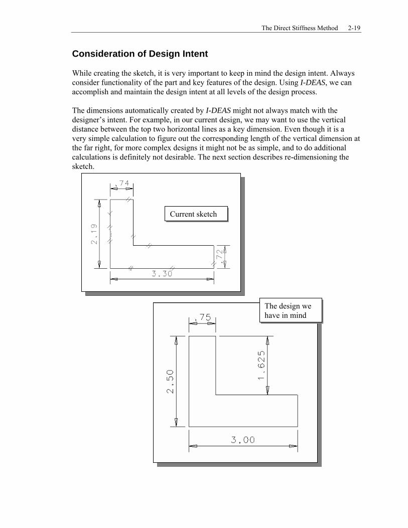
Consideration of Design Intent While creating the sketch, it is very important to keep in mind the design intent. Always consider functionality of the part and key features of the design. Using I-DEAS, we can accomplish and maintain the design intent at all levels of the design process. The dimensions automatically created by I-DEAS might not always match with the designer’s intent. For example, in our current design, we may want to use the vertical distance between the top two horizontal lines as a key dimension. Even though it is a very simple calculation to figure out the corresponding length of the vertical dimension at the far right, for more complex designs it might not be as simple, and to do additional calculations is definitely not desirable. The next section describes re-dimensioning the sketch.

Current sketch

The design we have in mind


Step 2: Apply/Delete/Modify constraints and dimensions

As the sketch is made, I-DEAS automatically applies some of the geometric constraints (such as horizontal, parallel and perpendicular) to the sketched geometry. We can continue to modify the geometry, apply additional constraints, and/or define the size of the existing geometry. In this example, we will illustrate deleting existing dimensions and add new dimensions to describe the sketched entities. To maintain our design intent, we will first remove the unwanted dimension and then create the desired dimension.

1. Pick Delete in the icon panel. (The icon is located in the

last row of the application icon panel.)

2. Pick the dimension as shown.

3. Press the ENTER key or the middle-mouse-button to accept the selection.

4. In the prompt window, the message “OK to delete 1 dimension?” is

displayed. Pick Yes in the popup menu, or press the ENTER key or the middle-mouse-button to delete the selected dimension. End the Delete command by hitting the middle-mouse-button again.

Delete this dimension


Creating Desired Dimensions

1. Choose Dimension in the icon panel. The message “Pick

the first entity to dimension” is displayed in the prompt window.

2. Pick the top horizontal line as shown in the figure below.

3. Pick the second horizontal line as shown.

4. Place the text to the right of the model.

5. Press the ENTER key or the middle-mouse-button to end the Dimension

command.

In I-DEAS, the Dimension command will create a linear dimension if two parallel lines are selected (distance in between the two lines). Selecting two lines that are not parallel will create an angular dimension (angle in between the two lines).

2. Pick the top horizontal line as the 1st entity to dimension

4. Position the dimension text

3. Second entity to dimension


Modifying Dimensional Values Next we will adjust the dimensional values to the desired values. One of the main advantages of using a feature-based parametric solid modeler, such as I-DEAS, is the ability to easily modify existing entities. The operation of modifying dimensional values will demonstrate implementation of the design philosophy of “shape before size.” In I-DEAS, several options are available to modify dimensional values. In this lesson, we will demonstrate two of the options using the Modify command. The Modify command icon is located in the second row of the application icon panel; the icon is a picture of an arrowhead with a long tail.

1. Choose Modify in the icon panel. (The icon is located in the second row of

the application icon panel. If the icon is not on top of the stack, press and hold down the left-mouse-button on the displayed icon, then select the Modify icon.) The message “Pick entity to modify” is displayed in the prompt window.

2. Pick the dimension as shown (the number might be different than displayed).

The selected dimension will be highlighted. The Modify Dimension window appears.

Modify this dimension.


In the Modify Dimension window, the value of the selected dimension is displayed and also identified by a name in the format of “Dxx,” where the “D” indicates it is a dimension and the “xx” is a number incremented automatically as dimensions are added. You can change both the name and the value of the dimension by clicking and typing in the appropriate boxes.

3. Type in 3.0 to modify the dimensional value as shown in the figure above.

4. Click on the OK button to accept the value you have entered.

I-DEAS will adjust the size of the object based on the new value entered.

5. On your own, click on the top horizontal dimension and adjust the

dimensional value to 0.75.

6. Press the ENTER key or the middle-mouse-button to end the Modify command.

3. Enter 3.0


The size of our design is

automatically adjusted by I-DEAS based on the dimensions we have entered. I-DEAS uses the dimensional values as control variables and the geometric entities are modified accordingly. This approach of rough sketching the shape of the design first then finalizing the size of the design is known as the “shape before size” approach.

Pre-selection of Entities I-DEAS provides a flexible graphical user interface that allows users to select graphical entities BEFORE the command is selected (pre-selection), or AFTER the command is selected (post-selection). The procedure we have used so far is the post-selection option. To pre-select one or more items to process, hold down the SHIFT key while you pick. Selected items will stay highlighted. You can deselect an item by selecting the item again. The item will be toggled on and off by each click. Another convenient feature of pre-selection is that the selected items remain selected after the command is executed.

1. Pre-select all of the dimensions by holding down the SHIFT key and clicking the left-mouse-button on each dimension value.

PRE-SELECT SHIFT + LEFT-mouse-button

2. Select the Modify icon. The Dimensions window

appears.


3. Move the Dimensions window around so that it does not overlap the part drawing. Do this by “clicking and dragging” the window’s title area with the left-mouse-button. You can also use the Dynamic Viewing functions (activate the graphics window first) to adjust the scale and location of the entities displayed in the graphics window (F1 and the mouse, F2 and the mouse).

4. Click on one of the dimensions in

the pop-up window. The selected dimension will be highlighted in the graphics window. Type in the desired value for the selected dimension. DO NOT hit the ENTER key. Select another dimension from the list to continue modifying. Modify all of the dimensional values to the values as shown.

5. Click the OK button to accept the

values you have entered and close the Dimensions window.

I-DEAS will now adjust the size of the shape to the desired dimensions. The design philosophy of “shape before size” is implemented quite easily. The geometric details are taken care of by I-DEAS.

Modify highlighted dimension.

Use the Dynamic Viewing functions to adjust location and/or size of the sketch.

Click and drag in the title area with left-mouse-button to move the Dimensions window.

Pick Dimensions to modify.


Step 3: Completing the Base Solid Feature ♦ Now that the 2D sketch is completed, we will proceed to the next step: create a 3D

feature from the 2D profile. Extruding a 2D profile is one of the common methods that can be used to create 3D parts. We can extrude planar faces along a path.

1. Choose Extrude in the icon panel. The Extrude icon is

located in the fifth row of the task specific icon panel. Press and hold down the left-mouse-button on the icon to display all the choices. If a different choice were to be made, you would slide the mouse up and down to switch between different options. In the prompt window, the message “Pick curve or section” is displayed.

2. Pick any edge of the 2D shape. By default, the Extrude

command will automatically select all segments of the shape that form a closed region. Notice the different color signifying the selected segments.

3. Notice the I-DEAS prompt “Pick curve to add or remove. (Done)” We can

select more geometric entities or deselect any entity that has been selected. Picking the same geometric entity will again toggle the selection of the entity “on” or “off” with each left-mouse-button click. Press the ENTER key to accept the selected entities.

4. The Extrude Section window will

appear on the screen. Enter 2.5, in the first value box, as the extrusion distance, and confirm that the New part option is set as shown in the figure.

5. Click on the OK button to accept

the settings and extrude the 2D section into a 3D solid.

Notice all of the dimensions disappeared from the screen. All of the dimensional values and geometric constraints are stored in the database by I-DEAS and they can be brought up at any time.


Display Viewing Commands

3D Dynamic Rotation – F3 and the mouse The I-DEAS Dynamic Viewing feature allows users to do “real-time” rotation of the display. Hold the F3 function key down and move the mouse to rotate the display. This allows you to rotate the displayed model about the screen X- (horizontal), Y- (vertical), and Z- (perpendicular to the screen) axes. Start with the cursor near the center of the screen and hold down F3; moving the cursor up or down will rotate about the screen X-axis while moving the cursor left or right will control the rotation about the screen Y-axis. Start with the cursor in the corner of the screen and hold down F3, which will control the rotation about the screen Z-axis.

Dynamic Rotation F3 + MOUSE Display Icon Panel The Display icon panel contains various icons to handle different viewing operations. These icons control the screen display, such as the view scale, the view angle, redisplay, and shaded and hidden line displays.

Top View

Refresh

Front View

Zoom All

Wireframe Image

Shaded Image

Zoom In

Isometric View

Side View


View icons: Front, Side, Top, Bottom, Isometric, and Perspective: These six icons are the standard view icons. Selecting any of these icons will change the viewing angle. Try each one as you read its description below

Front View (X-Y Workplane) Right Side View

Top View Bottom View

Isometric View Perspective View

Shaded Solids: Depending on your display type, you will pick either Shaded Hardware or Shaded Software to get shaded images of 3D objects. Shaded Hardware on a workstation with OGL display capability allows real-time dynamic rotation (F3 and the mouse) of the shaded 3D solids. A workstation with X3D display capability allows the use of the Shaded Software command to get the shaded image without the real-time dynamic rotation capability.

Shaded Hardware Shaded Software


Hidden-line Removal: Three options are available to generate images with all the back lines removed.

Hidden Hardware Precise Hidden Quick Hidden

Wireframe Image: This icon allows the display of the 3D objects using the basic wireframe representation scheme.

Wireframe

Refresh and Redisplay:

Use these commands to regenerate the graphics window.

Refresh Redisplay

Zoom-All: Adjust the viewing scale factor so that all objects are displayed.

Zoom-All

Zoom-In: Allows the users to define a rectangular area, by selecting two diagonal corners, which will fill the graphics window.

Zoom-In


Workplane – It is an XY CRT, but an XYZ World

Design modeling software is becoming more powerful and user friendly, yet the system still does only what the user tells it to do. In using a geometric modeler, therefore, we need to have a good understanding of what the inherent limitations are. We should also have a good understanding of what we want to do and what results to expect based upon what is available. In most 3D geometric modelers, 3D objects are located and defined in what is usually called world space or global space. Although a number of different coordinate systems can be used to create and manipulate objects in a 3D modeling system, the objects are typically defined and stored using the world space. The world space is usually a 3D Cartesian coordinate system that the user cannot change or manipulate. In most engineering designs, models can be very complex; it would be tedious and confusing if only the world coordinate system were available. Practical 3D modeling systems allow the user to define Local Coordinate Systems or User Coordinate Systems relative to the world coordinate system. Once a local system is defined, we can then create geometry in terms of this more convenient system. Although objects are created and stored in 3D space coordinates, most of the input and output is done in a 2D Cartesian system. Typical input devices such as a mouse or digitizers are two-dimensional by nature; the movement of the input device is interpreted by the system in a planar sense. The same limitation is true of common output devices, such as CRT displays and plotters. The modeling software performs a series of three-dimensional to two-dimensional transformations to correctly project 3D objects onto the 2D picture plane (monitor).


The I-DEAS workplane is a special construction tool that enables the planar nature of 2D input devices to be directly mapped into the 3D coordinate system. The workplane is a local coordinate system that can be aligned to the world coordinate system, an existing face of a part, or a reference plane. By default, the workplane is aligned to the world coordinate system. The basic design process of creating solid features in the I-DEAS task is a three-step process:

1. Select and/or define the workplane. 2. Sketch and constrain 2D planar geometry. 3. Create the solid feature.

These steps can be repeated as many times as needed to add additional features to the design. The base feature of the Adjuster Block model was created following this basic design process; we used the default settings where the workplane is aligned to the world coordinate system. We will next add additional features to our design and demonstrate how to manipulate the I-DEAS workplane. Workplane Appearance The workplane is a construction tool; it is a coordinate system that can be moved in space. The size of the workplane display is only for our visual reference, since we can sketch on the entire plane, which extends to infinity.

1. Choose Workplane Appearance in

the icon panel. (The icon is located in the second row of the application icon panel. If the icon is not on top of the stack, press and hold down the left-mouse-button on the displayed icon to display all the choices, then select the Workplane Appearance icon.) The Workplane Attributes window appears.


2. Toggle on the three display switches as shown.

3. Adjust the workplane border size by entering the Min. and Max. values as

shown.

4. In the Workplane Attributes window, click on the Workplane Grid button. The Grid Attributes window appears.

5. Change the Grid Size settings by entering the values as shown.

6. Toggle on the Display Grid option if it is not already switched on.

Although the Grid Snap option is available, its usage in parametric modeling is not

recommended. The Grid Snap concept does not conform to the “shape before size” philosophy and most real designs rarely have uniformly spaced dimension values.

7. Pick Apply to view the effects of the changes.

8. Click on the OK button to exit the Grid Attributes window.

9. Click on the OK button to exit the Workplane Attributes window.

10. On your own, use [F3+Mouse] to dynamically rotate the part and observe the

workplane is aligned with the surface corresponding to the first sketch drawn.

2. Display switches

3. Border size 4. Grid controls

5. Grid size & display 6.Toggle ON


Step 4: Adding additional features

Sketch in Place One option to manipulate the workplane is with the Sketch in Place command. The Sketch in Place command allows the user to sketch on an existing part face. The workplane is reoriented and is attached to the face of the part.

1. Choose Isometric View in the

display viewing icon panel. 2. Choose Zoom-All in the display

viewing icon panel.

3. Choose Sketch in Place in the icon panel. In the prompt

window, the message “Pick plane to sketch on” is displayed. 4. Pick the top face of the horizontal portion of the 3D object

by left-clicking the surface, when it is highlighted as shown in the figure below.

Notice that, as soon as the top surface is picked, I-DEAS automatically orients the workplane to the selected surface. The surface selected is highlighted with a different color to indicate the attachment of the workplane.

4. Pick the top face of the base feature.


Step 4-1: Adding an extruded feature

Next, we will create another 2D sketch, which will be used to create an extruded feature that will be added to the existing solid object.

1. Choose Rectangle by 2 Corners in the icon

panel. This command requires the selection of two locations to identify the two opposite corners of a rectangle. The message “Locate first corner” is displayed in the prompt window.

2. Create a rectangle by first selecting the top

left corner of the solid model as shown in the figure. Note that I-DEAS automatically snaps to the end points of existing geometry.

3. Create a rectangle of arbitrary size by

selecting a location that is toward the front left direction of the last location as shown in the figure.

Note that I-DEAS automatically applies

dimensions as the rectangle is constructed. Do not be concerned with the actual numbers of the dimensions, which we will adjust in the next section.


4. On your own, modify the two

dimensions to 0.75 and 2.25 as shown in the figure.

5. Choose Extrude in the icon panel. The Extrude

icon is located in the fifth row of the task specific icon panel.

6. In the prompt window, the message “Pick curve or section” is

displayed. Pick the front edge of the 2D rectangle we just created. By default, the Extrude command will automatically select all neighboring segments of the selected segment to form a closed region. Notice the different color signifying the selected segments.

7. Pick the segment in between the displayed two small circles so that the highlighted entities form a closed region.


8. The short segment of the sketched rectangle, aligned to the top edge of the solid model, is highlighted and notice the double line cursor is displayed. Press the ENTER key once, or click once with the middle-mouse-button, to accept the selected entity.

Attempting to select a line where two entities lie on top of one another (i.e., coincide)

causes confusion as indicated by the double line cursor ╬ symbol and the prompt window message “Pick curve to add or remove (Accept)**”. This message indicates I-DEAS needs you to confirm the selected item. If the correct entity is selected, you can continue to select additional entities. To reject an erroneously selected entity, press the [F8] key to select a neighboring entity or press the right-mouse-button and highlight Deselect All from the popup menu.

9. Confirm the four sides of the sketched rectangle are highlighted and press the

ENTER key once, or click once with the middle-mouse-button, to proceed with the Extrude command.

10. The Extrude window appears on the screen. Click on the Flip

Direction button near the upper right corner of the Extrude window to switch the extrusion direction so that the green arrow points downward.

11. Enter 2.5, in the first value box, as

the extrusion distance.

12. Confirm that the Join option is set as shown in the figure.


13. Confirm the extrusion options inside the Extrude window and the displayed image inside the graphics window are set as shown.

14. Click on the OK button to accept the settings and extrude the sketched 2D

section into a 3D solid feature of the solid model.


Step 4-2: Adding a cut feature • Next, we will create a circular cut feature to the existing solid object.

1. Choose Isometric View in the

display viewing icon panel. 2. Choose Zoom-All in the display

viewing icon panel.

3. Choose Sketch in Place in the icon panel. In the prompt

window, the message “Pick plane to sketch on” is displayed. 4. Pick the top face of the horizontal portion of the 3D object

by left-clicking the surface, when it is highlighted as shown in the figure below.

4. Pick this face of the base feature.


5. Choose Circle – Center Edge in the icon panel. This

command requires the selection of two locations: first the location of the center of the circle and then a location where the circle will pass through.

6. On your own, create a circle inside the

horizontal face of the solid model as shown.

7. On your own, create and

modify the three dimensions as shown.


♦ Extrusion – Cut option

1. Choose Extrude in the icon panel. The Extrude icon is

located in the fifth row of the task specific icon panel. 2. In the prompt window, the message “Pick curve or section” is

displayed. Pick the newly sketched circle. 3. At the I-DEAS prompt “Pick curve to add or remove (Done),”

press the ENTER key or the middle-mouse-button to accept the selection.

4. The Extrude Section window appears. Set the

extrude option to Cut. Note the extrusion direction displayed in the graphics window.

5. Click and hold down the left-mouse-button on

the depth menu and select the Thru All option. I-DEAS will calculate the distance necessary to cut through the part.

6. Click on the OK button to accept the settings.

The rectangle is extruded and the front corner of the 3D object is removed.


7. On your own, create another circular cut feature on the vertical section and complete the model as shown.

Save the Part and Exit I-DEAS

1. From the icon panel, select the File pull-down

menu. Pick the Save option. Notice that you can also use the Ctrl-S combination (pressing down the Ctrl key and hitting the “S” key once) to save the part. A small watch appears to indicate passage of time as the part is saved.

2. Now you can leave I-DEAS. Use the left-mouse-

button to click on File in the toolbar menu and select Exit from the pull-down menu. A pop-up window will appear with the message “Save changes before exiting?” Click on the NO button since we have saved the model already.


Questions: 1. The truss element used in finite element analysis is considered as a two-force member

element. List and describe the assumptions of a two-force member. 2. What is the size of the stiffness matrix for a single element? What is the size of the

overall global stiffness matrix in example 2.2? 3. What is the first thing we should setup when building a new CAD model in I-DEAS? 4. How does the I-DEAS Dynamic Navigator assist us in sketching? 5. How do we remove the dimensions created by the Dynamic Navigator? 6. How do we modify more than one dimension at a time? 7. What is the difference between Distance and Thru All when extruding? 8. Identify and describe the following commands:

(a)

SHIFT + LEFT mouse button (b)

(c)

(d)

F3 + Mouse


Exercises: 1. Determine the nodal displacements and reaction forces using the direct stiffness

method.

2.

F = 60 lbs.

K1= 50 lb/in K2 = 60 lb/in

+X

Node 1 Node 2 Node 3

K3 = 55 lb/in

Node 4


Notes: