SPEECH ENHANCEMENT USING AN MMSE SPECTRAL AMPLITUDE ESTIMATORBASED ON A MODULATION DOMAIN KALMAN FILTER WITH A GAMMA PRIOR
Yu Wang? Mike Brookes†
?Engineering Department, University of Cambridge, United Kingdom†Department of Electrical and Electronic Engineering, Imperial Collge London, United Kingdom
[email protected] [email protected]
ABSTRACT
In this paper, we propose a minimum mean square error spectralestimator for clean speech spectral amplitudes that uses a Kalmanfilter to model the temporal dynamics of the spectral amplitudes inthe modulation domain. Using a two-parameter Gamma distributionto model the prior distribution of the speech spectral amplitudes, wederive closed form expressions for the posterior mean and varianceof the spectral amplitudes as well as for the associated update stepof the Kalman filter. The performance of the proposed algorithmis evaluated on the TIMIT core test set using the perceptual evalua-tion of speech quality (PESQ) measure and segmental SNR measureand is shown to give a consistent improvement over a wide range ofSNRs when compared to competitive algorithms.
Index Terms— speech enhancement, modulation domain Kalmanfilter, minimum mean-square error (MMSE) estimator
1. INTRODUCTION
Over several decades, numerous speech enhancement algorithmshave been proposed. Among the most popular are those such as[1, 2, 3] which apply a variable gain in the short time Fourier trans-form (STFT) domain to estimate the spectral amplitudes of theclean speech. Although these STFT-domain enhancement algo-rithms often improve the signal-to-noise ratio (SNR) dramatically,the temporal dynamics of the speech spectral amplitudes are notincorporated into the derivation of the estimator. There is evidence,however, that significant information in speech is carried by themodulation of spectral envelopes in addition to the envelopes them-selves [4, 5]. Spectral modulation-domain processing has been usedin speech recognition [6, 7], in speech intelligibility metrics [8, 9]and in speech enhancement [10, 11, 12]. In one such enhancementalgorithm [12], the temporal envelope of the amplitude spectrumof the noisy speech is processed separately in each subband by aKalman filter (KF) in order to obtain the spectral amplitudes of theenhanced speech. This modulation-domain KF combines the esti-mated dynamics of the speech spectral amplitudes with the observednoisy speech amplitudes to give an minimum mean square error(MMSE) estimate of the amplitude spectrum of the clean speech,under the assumption that the spectral amplitudes of both the cleanspeech and the noise are Gaussian distributed.
In this paper, we propose an MMSE spectral amplitude estima-tor under the assumption that the speech amplitudes follow a gen-eralized Gamma distribution [13]. The advantage of the proposed
Yu Wang was a PhD student at Imperial College London during thecourse of this work.
estimator over previously proposed spectral amplitude estimators[2, 13, 14] is that it incorporates temporal continuity into the MMSEestimator by the use of the KF and that it uses a Gamma prior whichis a more appropriate model for the speech spectral amplitudes thana Gaussian prior [11].
2. SIGNAL MODEL AND KALMAN FILTER
We assume an additive model in the STFT domain in which, forfrequency bin k of frame n,
Yn,k = Xn,k +Wn,k (1)
where X and W denote the complex-valued STFT coefficients ofthe clean speech and the noise respectively. Since each frequencybin is processed independently within our algorithm, we omit thefrequency index, k, in the remainder of this paper. We denote thespectral amplitudes as: |Xn| = An, |Yn| = Rn and |Wn| = Nn.The prediction model we assume for the clean speech spectral am-plitudes is
an = Fn�1an�1 + vn (2)
where an = [An · · ·An�p+1]T is the p-dimensional state vec-
tor and vn denotes the zero-mean prediction residual with co-variance matrix Qn. The (p ⇥ p) transition matrix has the form
Fn =
�bT
nI 0
�, where bn = [b1 · · · bp]T is the vector of linear
prediction (LPC) coefficients for the speech spectral amplitudes inframe n. Our model differs from that used in [12] in two respects:we treat the noise and speech as additive in the complex STFTdomain rather than in the spectral amplitude domain and we use ageneralized Gamma prior for the speech amplitudes rather than aGaussian prior.
3. PROPOSED ESTIMATOR DESCRIPTION
A block diagram of the proposed algorithm is shown in Fig. 1.The noisy speech, y(t) is converted to the time-frequency do-main, Rn,ke
j⇥n,k, using the STFT [15]. In order to perform LPCmodelling in the modulation domain, the noise power spectrum isestimated using, for example, [16] or [17], and the speech is passedthrough a conventional MMSE enhancer [3] to reduce the effects ofthe noise on the modelling. Following this, the sequence of spec-tral amplitudes in each frequency bin is divided into overlappingmodulation frames. Autocorrelation LPC [18] is performed on eachmodulation frame to determine the coefficients, bn, and thence thetransition matrix Fn in (2).
STFT$KF$Update$$
$$$Noise$$Es1mator$
logMMSE$enhancer$
KF$Predict$$
Modula1on$Domain$LPC$
ISTFT$
1Aframe$delay$$
y(t)Yn,k
�n,k x̂(t)
�2n,k
�2n,k
an|n�1
Pn|n�1
an|n Pn|n
Pn�1|n�1
an�1|n�1
Fn
bn
Fig. 1. Block diagram of the proposed Kalman Filter MMSE esti-mator.
3.1. Kalman filter prediction step
From the time update model (2), we obtain the KF prediction equa-tions
an|n�1 = Fn�1an�1|n�1 (3)
Pn|n�1 = Fn�1Pn�1|n�1FTn�1 +Qn, (4)
where an|n�1 and Pn|n�1 denote respectively the a priori estimatesof the amplitude state vector and of the corresponding covariancematrix at time n, and an�1|n�1 denotes the a posteriori estimate ofthe state vector at time n � 1. The first element of the state vector,an|n�1, corresponds to the spectral amplitude in the current frame,An|n�1, and so its a priori mean and variance are given by
µn|n�1 , E(An|Rn�1) = dTan|n�1 (5)
�2n|n�1 , V ar(An|Rn�1) = cTPn|n�1c, (6)
where Rn�1 represents the observed speech amplitudes up to timen� 1 and c = [1 0...0]T .
3.2. Kalman Filter MMSE update model
In this section, we describe the KF MMSE update step which de-termines an updated state estimate by combining the predicted statevector and covariance, the estimated noise and the observed spec-tral amplitude. Within the update step, we model the prior speechamplitude An|n�1 using a 2-parameter Gamma distribution
p (an|Rn�1) =2a2�n�1
n
�2�nn � (�n)
exp
✓�a2
n
�2n
◆, (7)
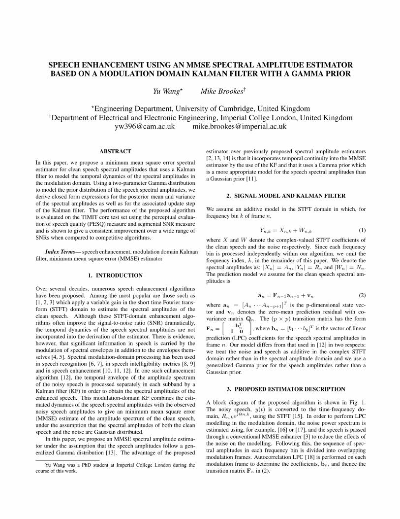
where � (·) is the Gamma function. The distribution is obtainedby setting c = 2 in the generalized Gamma distribution given in[19], and the two parameters, �n and �n are chosen to match themean µn and variance �2
n of the predicted amplitude from (5) and(6). Examples of the probability density functions from (7) withvariance, �2
= 1 and means, µ, in the range 0.5 to 8 are shownin Fig. 2, from which it can be seen that the distribution in (7) issufficiently flexible to model the outcome of the prediction over awide range of µn/�n.
At frame n, the mean and variance of the Gamma distribution in(7) can be expressed in terms of �n and �n [19] as
0 2 4 6 8 100
0.2
0.4
0.6
0.8
1
a
p(a
)
µ=0.5, σ=1.0
µ=1.0, σ=1.0
µ=1.5, σ=1.0
µ=4.0, σ=1.0
µ=8.0, σ=1.0
Fig. 2. Curves of Gamma probability density function for (7) withvariance �2
= 1 and different means.
0 0.2 0.4 0.6 0.8 10
0.5
1
1.5
λ
φ
true
fitted
Fig. 3. The curve of � versus �, where 0 < � = arctan(�) < ⇡2
and 0 < � =
�2(�+0.5)�2(�)�
< 1.
µn|n�1 = �n� (�n + 0.5)
� (�n), (8)
�2n|n�1 = �2
n
✓�n � �
2(�n + 0.5)�
2(�n)
◆. (9)
We can eliminate � between (8) and (9) to obtain
�
2(�n + 0.5)
�n�2(�n)
=
µ2n|n�1
µ2n|n�1 + �2
n|n�1
, �n (10)
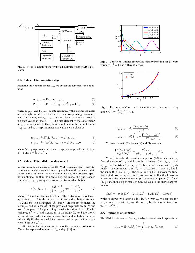
We need to solve the non-linear equation (10) to determine �nfrom the value of �n which can be calculated from µn|n�1 and�2n|n�1 and satisfies 0 < �n < 1. Instead of dealing with �n di-
rectly, it is convenient to set �n = arctan(�n) where �n lies inthe range 0 < �n < ⇡
2 . The solid line in Fig. 3 shows the func-tion �n(�). We can approximate this function well with a low-orderpolynomial that is constrained to pass through the points (0, 0) and(1, ⇡
2 ) and in the experiments in Sec. 4.1 we use the quartic approx-imation
�(�) = �0.1640�4+ 2.3612�3 � 1.2182�2
+ 0.5918�
which is shown with asterisks in Fig. 3. Given �n we can use thispolynomial to obtain �n and thence �n by the inverse transform�n = tan(�n).
3.3. Derivation of estimator
The MMSE estimate of An is given by the conditional expectation
µn|n = E(An|Rn) =
1̂
0
anp(an|Rn)dan (11)
Using Bayes rule, the conditional probability is expressed as
p (an|Rn) = p(an|yn,Rn�1)
=
´ 2⇡
0p (yn|an,�n,Rn�1) p (an,�n|Rn�1) d�n
p (yn|Rn�1)
(12)
where �n is the realization of the random variable �n which rep-resents the phase of the clean speech. Because Yn is conditionallyindependent of Rn�1 given an and �n, (12) becomes
p (an|Rn) =
´ 2⇡0
p (yn|an,�n) p (an,�n|Rn�1) d�n
p (yn|Rn�1)(13)
Following [2], the observation noise is assumed to be complex Gaus-sian distributed with variance ⌫2
n = E(N2n) leading to the observa-
tion prior model
p(yn|an,�n) =1
⇡⌫2nexp
⇢� 1
⌫2n|yn � ane
j�n |2�
(14)
Under the assumption of the statistical models previously definedand assuming that the phase components and amplitude components,�n and An, are independent, we can now calculate a closed-formexpression for the estimator (11) using [20, Eq. 6.631, 9.201.1,9.220.2]
µn|n =
� (�n + 0.5)� (�n)
s⇠n
⇣n(�n + ⇠n)
M⇣�n + 0.5; 1; ⇣n⇠n
�n+⇠n
⌘
M⇣�n; 1;
⇣n⇠n�n+⇠n
⌘ Rn,
(15)where M is the confluent hypergeometric function [21], and
⇠n =
E(A2n|Yn�1)
⌫2n
=
µ2n|n�1 + �2
n|n�1
⌫2n
, ⇣n =
R2n
⌫2n
are the a priori SNR and a posteriori SNR respectively. The varianceof the posterior estimate is given by
�2n|n = E
�A2
n|Rn,�n
�� (E (An|Rn,�n))
2
=
�n⇠n⇣n(�n + ⇠n)
M⇣�n + 1; 1;
⇣n⇠n�n+⇠n
⌘
M⇣�n; 1;
⇣n⇠n�n+⇠n
⌘ R2n �
�µn|n
�2 .
(16)
3.4. Update of state vector
The final step is to update the entire state vector and the associatedcovariance matrix, an|n and Pn|n. In order to decorrelate the cur-rent observation from the rest of the state vector, we decompose thecovariance matrix Pn|n�1 as
Pn|n�1 =
�2n|n�1 gT
n
gn Gn
�,
where gn is a (p � 1)-dimensional vector. We now transform thestate vector as
zn|n�1 = Hnan|n�1 (17)
using the transformation matrix Hn =
"1 0T
� gn�2n|n�1
I
#. The
covariance matrix, Un|n�1, of the transformed state vector zn|n�1
is given by
Un|n�1 = E⇣zn|n�1z
Tn|n�1
⌘= HnPn|n�1H
Tn
=
"�2n|n�1 0T
0 Gn � ��2n|n�1gngT
n
#.
We see that the first element of zn|n�1 is equal to µn|n�1 and un-correlated with any of the other elements and is therefore distributedas N (µn|n�1,�
2n|n�1). Using the posterior mean and variance from
(15) and (16) and c = [1 0 . . . 0]T , we can update the transformedmean vector and covariance matrix as
zn|n = zn|n�1 + (µn|n � µn|n�1)c
Un|n = Un|n�1 +��2n|n � �2
n|n�1
�ccT .
Inverting the transformation in (17), we obtain, after some alge-braic manipulation, the following update equations
an|n = an|n�1 +�µn|n � µn|n�1
���2n|n�1Pn|n�1c (18)
Pn|n = Pn|n�1 +
⇣�2n|n�
�2n|n�1 � 1
⌘��2n|n�1Pn|n�1cc
TPn|n�1.
(19)
In this section we have derived the update equations for the KF.For each acoustic frame of noisy speech, we first use (3) and (4)to calculate the a priori state vector an|n�1 and the correspondingcovariance Pn|n�1, and solve (10) to find �n. We then use (15) and(16) to calculate the a posteriori estimate of the amplitude and thecorresponding variance respectively. Finally, the KF state vector andits covariance matrix are updated using (18) and (19).
4. IMPLEMENTATION AND EVALUATION
4.1. Implementation of algorithm
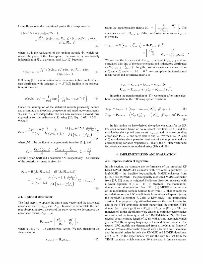
In this section, we compare the performance of the proposed KFbased MMSE (KMMSE) estimator with five other algorithms: (i)logMMSE – the baseline log-amplitude MMSE enhancer from[3, 22]; (ii) pMMSE – the perceptually motivated MMSE estimatorfrom [23, 22] using a weighted Euclidean distortion measure witha power exponent of p = �1; (iii) ModSub – the modulation-domain spectral subtraction from [11]; (iv) MDKF – the versionof the modulation-domain Kalman filter from [12] that extracts themodulation-domain LPC coefficients from enhanced speech (usingthe logMMSE algorithm [3, 22]); (v) KFMMSEI – an intermediateversion of our proposed algorithm that assumes the speech and noiseadd in the STFT amplitude domain rather than the complex STFTdomain (i.e. replacing (1) with |Yn,k| = |Xn,k|+ |Wn,k|). The pa-rameters of all the algorithms were chosen to optimize performanceon a subset of the training set of the TIMIT database [24]. We haveused an acoustic frame length of 32 ms with a 4 ms increment whichgives a 250 Hz sampling frequency in the modulation domain. Thespeech LPC models are determined from a modulation frame ofduration 128 ms (32 acoustic frames) with a 16 ms frame incrementand the model orders in both the KMMSE and MDKF algorithmsare l = 2. In the experiments, we use the core test set from theTIMIT database which contains 16 male and 8 female speakers
−10 −5 0 5 10 15−20
−15
−10
−5
0
5
10
15
Global SNR of noisy speech (dB)
segS
NR
(dB
)
KMMSEpMMSEMDKFlogMMSENoisy
−10 −5 0 5 10 15−20
−15
−10
−5
0
5
10
15
Global SNR of noisy speech (dB)
segS
NR
(dB
)
KMMSEpMMSEMDKFlogMMSENoisy
Fig. 4. Average segmental SNR of enhanced speech speech afterprocessing by four algorithms plotted against the global SNR of theinput speech corrupted by additive car noise (left) and street noise(right). The algorithm acronyms are defined in the text.
−10 −5 0 5 10 151.5
2
2.5
3
3.5
4
Global SNR of noisy speech (dB)
PE
SQ
KMMSEpMMSEMDKFlogMMSENoisy
−10 −5 0 5 10 151.5
2
2.5
3
3.5
4
Global SNR of noisy speech (dB)
PE
SQ
KMMSEpMMSEMDKFlogMMSENoisy
Fig. 5. Average PESQ quality of enhanced speech after processingby four algorithms plotted against the global SNR of the input speechcorrupted by additive car noise (left) and street nose (right).
each reading 8 distinct sentences (totalling 192 sentences) and thespeech is corrupted by the noise from the RSG-10 database [25] andthe ITU-T test signals database [26] at �10,�5, 0, 5, 10 and 15 dBglobal SNR. A Hamming window is used in the STFT analysis andsynthesis and the noise power spectrum, ⌫2
n,k, is estimated using thealgorithm from [17] as implemented in [22]. It is possible for thealgorithm to lock up with µn|n = 0; to prevent this, we impose theconstraint �n > 0.5 in (10).
4.2. Performance evaluations
The performance of the algorithms is evaluated using both segmen-tal SNR (segSNR) and the perceptual evaluation of speech quality(PESQ) measure defined in ITU-T P.862. All the measured val-
1.5
2
2.5
3
Noisy logMMSE pMMSE ModSub MDKF KMMSEI KMMSE
PE
SQ
Fig. 6. Box plot of the PESQ scores for noisy speech processed bysix enhancement algorithms. The plots show the median, interquar-tile range and extreme values from 2376 speech+noise combinations.
−1
−0.5
0
0.5
Noisy logMMSE pMMSE ModSub MDKF KMMSEI
∆P
ES
Q
KMMSE
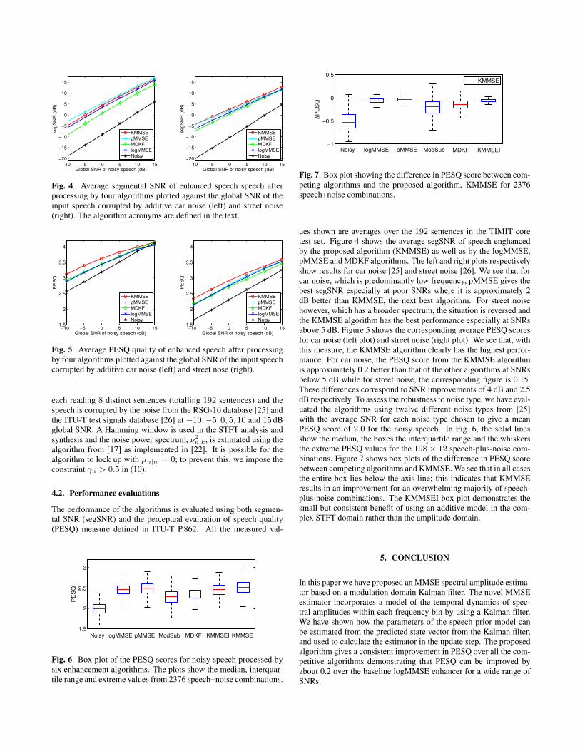
Fig. 7. Box plot showing the difference in PESQ score between com-peting algorithms and the proposed algorithm, KMMSE for 2376speech+noise combinations.
ues shown are averages over the 192 sentences in the TIMIT coretest set. Figure 4 shows the average segSNR of speech enghancedby the proposed algorithm (KMMSE) as well as by the logMMSE,pMMSE and MDKF algorithms. The left and right plots respectivelyshow results for car noise [25] and street noise [26]. We see that forcar noise, which is predominantly low frequency, pMMSE gives thebest segSNR especially at poor SNRs where it is approximately 2dB better than KMMSE, the next best algorithm. For street noisehowever, which has a broader spectrum, the situation is reversed andthe KMMSE algorithm has the best performance especially at SNRsabove 5 dB. Figure 5 shows the corresponding average PESQ scoresfor car noise (left plot) and street noise (right plot). We see that, withthis measure, the KMMSE algorithm clearly has the highest perfor-mance. For car noise, the PESQ score from the KMMSE algorithmis approximately 0.2 better than that of the other algorithms at SNRsbelow 5 dB while for street noise, the corresponding figure is 0.15.These differences correspond to SNR improvements of 4 dB and 2.5dB respectively. To assess the robustness to noise type, we have eval-uated the algorithms using twelve different noise types from [25]with the average SNR for each noise type chosen to give a meanPESQ score of 2.0 for the noisy speech. In Fig. 6, the solid linesshow the median, the boxes the interquartile range and the whiskersthe extreme PESQ values for the 198 ⇥ 12 speech-plus-noise com-binations. Figure 7 shows box plots of the difference in PESQ scorebetween competing algorithms and KMMSE. We see that in all casesthe entire box lies below the axis line; this indicates that KMMSEresults in an improvement for an overwhelming majority of speech-plus-noise combinations. The KMMSEI box plot demonstrates thesmall but consistent benefit of using an additive model in the com-plex STFT domain rather than the amplitude domain.
5. CONCLUSION
In this paper we have proposed an MMSE spectral amplitude estima-tor based on a modulation domain Kalman filter. The novel MMSEestimator incorporates a model of the temporal dynamics of spec-tral amplitudes within each frequency bin by using a Kalman filter.We have shown how the parameters of the speech prior model canbe estimated from the predicted state vector from the Kalman filter,and used to calculate the estimator in the update step. The proposedalgorithm gives a consistent improvement in PESQ over all the com-petitive algorithms demonstrating that PESQ can be improved byabout 0.2 over the baseline logMMSE enhancer for a wide range ofSNRs.
6. REFERENCES
[1] S. Boll. Suppression of acoustic noise in speech using spec-tral subtraction. IEEE Trans. Acoust., Speech, Signal Process.,27(2):113 – 120, April 1979.
[2] Y. Ephraim and D. Malah. Speech enhancement using aminimum-mean square error short-time spectral amplitudeestimator. IEEE Trans. Acoust., Speech, Signal Process.,32(6):1109–1121, December 1984.
[3] Y. Ephraim and D. Malah. Speech enhancement using aminimum mean-square error log-spectral amplitude estimator.IEEE Trans. Acoust., Speech, Signal Process., 33(2):443–445,1985.
[4] L. Atlas and S.A. Shamma. Joint acoustic and modulationfrequency. EURASIP Journal on Applied Signal Processing,7:668–675, 2003.
[5] R. Drullman, J. M. Festen, and R. Plomp. Effect of temporalenvelope smearing on speech reception. J. Acoust. Soc. Am.,95(2):1053–1064, 1994.
[6] H. Hermansky and N. Morgan. RASTA processing of speech.IEEE Transactions on Speech and Audio Processing, 2(4):578–589, 1994.
[7] B. E. D. Kingsbury, N. Morgan, and S. Greenberg. Robustspeech recognition using the modulation spectrogram. Speechcommunication, 25(1):117–132, 1998.
[8] C. H. Taal, R. C. Hendriks, R. Heusdens, and J. Jensen.An algorithm for intelligibility prediction of time frequencyweighted noisy speech. IEEE Trans. Audio, Speech, Lang. Pro-cess., 19(7):2125–2136, September 2011.
[9] R. L. Goldsworthy and J. E. Greenberg. Analysis of speech-based speech transmission index methods with implications fornonlinear operations. J. Acoust. Soc. Am., 116(6):3679–3689,December 2004.
[10] T. H. Falk, S. Stadler, W. B. Kleijn, and W. Y. Chan. Noisesuppression based on extending a speech-dominated modula-tion band. In Proc. Interspeech Conf., pages 970–973, August2007.
[11] K. Paliwal, K. Wojcicki, and B. Schwerin. Single-channelspeech enhancement using spectral subtraction in the short-time modulation domain. Speech Communication, 52(5):450–475, 2010. The Matlab software is available online at URL:http://maxwell.me.gu.edu.au/spl/research/modspecsub/.
[12] S. So and K. K. Paliwal. Modulation-domain Kalman filteringfor single-channel speech enhancement. Speech Communica-tion, 53(6):818–829, July 2011.
[13] J. S. Erkelens, R. C. Hendriks, R. Heusdens, and J. Jensen.Minimum mean-square error estimation of discrete fourier co-efficients with generalized gamma priors. IEEE Trans. SpeechAudio Process., 15(6):1741–1752, 2007.
[14] R. Martin. Speech enhancement based on minimum mean-square error estimation and supergaussian priors. IEEE Trans.Speech Audio Process., 13(5):845–856, September 2005.
[15] J. R. Deller, J. G. Proakis, and J. H. L. Hansen. Discrete TimeProcessing of Speech Signals. Prentice Hall, 1993.
[16] R. Martin. Noise power spectral density estimation basedon optimal smoothing and minimum statistics. IEEE Trans.Speech Audio Process., 9(5):504 –512, July 2001.
[17] T. Gerkmann and R. C. Hendriks. Unbiased MMSE-basednoise power estimation with low complexity and low track-ing delay. IEEE Trans. Audio, Speech, Lang. Process.,20(4):1383–1393, May 2012.
[18] J. Makhoul. Linear prediction: A tutorial review. Proceedingsof the IEEE, 63(4):561 – 580, April 1975.
[19] L. Norman, S. Kotz, and N. Balakrishnan. Continuous Uni-variate Distributions. Wiley, 1994.
[20] A. Jeffrey and D. Zwillinger. Table of Integrals, Series, andProducts. Academic Press, 2007.
[21] F. Olver, D. Lozier, R. F. Boiszert, and C. W. Clark, editors.NIST Handbook of Mathematical Functions: Companion tothe Digital Library of Mathematical Functions. CambridgeUniversity Press, 2010. URL: http://dlmf.nist.gov/13.
[22] D. M. Brookes. VOICEBOX: A speech processing tool-box for MATLAB. http://www.ee.imperial.ac.uk/hp/staff/dmb/voicebox/voicebox.html, 1998-2014.
[23] P. C. Loizou. Speech enhancement based on perceptually mo-tivated Bayesian estimators of the magnitude spectrum. IEEETrans. Speech Audio Process., 13(5):857–869, 2005.
[24] J. S. Garofolo, L. F. Lamel, W. M. Fisher, J. G. Fiscus, D. S.Pallett, N. L. Dahlgren, and V. Zue. TIMIT acoustic-phoneticcontinuous speech corpus. Corpus LDC93S1, Linguistic DataConsortium, Philadelphia, 1993.
[25] H. J. M. Steeneken and F. W. M. Geurtsen. Description of theRSG.10 noise data-base. Technical Report IZF 1988–3, TNOInstitute for perception, 1988.
[26] ITU-T P.501. Test signals for use in telephonometry, August1996.
Recommended