Shortest Paths for Line Segments∗

Christian Icking∗∗ Gunter Rote† Emo Welzl‡ Chee Yap§

February 3, 1992

Abstract

We study the problem of shortest paths for a line segment in the plane.As a measure of the distance traversed by a path, we take the average curvelength of the orbits of prescribed points on the line segment. This problem isnontrivial even in free space (i.e., in the absence of obstacles). We characterizeall shortest paths of the line segment moving in free space under the measured2, the average orbit length of the two endpoints.

The problem of d2 optimal motion has been solved by Gurevich and alsoby Dubovitskij, who calls it Ulam’s problem. Unlike previous solutions, ourbasic tool is Cauchy’s surface-area formula. This new approach is relativelyelementary, and yields new insights.

1 Introduction

The problem of moving an object amidst obstacles has received considerable atten-tion recently. Most of these results are concerned with the feasibility of an obstacle-avoiding motion (see for example [SchSh, Yap]). The problem of optimal motionshas also been studied although the results here are almost exclusively for the caseof moving a sphere (including the limiting case of moving a point). See for example[AAGHI]. The main reason for this paucity of results for moving non-spherical ob-jects is that one must now contend with motions that are neither pure translationsnor pure rotations — such motions apparently defeat the known techniques in thefield of computational geometry. Furthermore, there is no well-accepted definition ofmeasuring the distance traversed by a motion of general objects. One obvious sug-gestion for the case of moving a line segment turns out to be a bad idea: to take thearea swept by the motion of the line segment. In this case, it was shown that the area

∗This work was partially supported by the ESPRIT II Basic Research Actions Program of theEC under contract no. 3075 (project ALCOM) and by the Deutsche Forschungsgemeinschaft grantOt 64/5-3. Chee Yap acknowledges support from the Deutsche Forschungsgemeinschaft, and partialsupport from NSF grants DCR-8401898 and DCR-8401633.

∗∗FernUniversitat Hagen, Praktische Informatik VI, D-5800 Hagen†Technische Universitat Graz, Institut fur Mathematik, Kopernikusgasse 24, A-8010 Graz‡Freie Universitat Berlin, Institut fur Informatik, Arnimallee 2–6, D-1000 Berlin 33§Courant Institute, New York University

1

swept by a motion of the line segment that performs a ‘180 degrees turn, in place’can be arbitrarily close to zero (see Besicovitch [Bes], who attributes this problem toKakeya).

Nevertheless, there is some agreement (e.g., [PaSi, ORo]) that one natural measureon motions is the average distance traversed by each point on the object. In thispaper, we call this the natural measure and denote it by d∞ (see Section 2). Thetrouble is that there are no known tools for studying d∞-optimal motions, even infree space. To get around this, one must either restrict the allowable motions (as in[ORo]) or change the measure ([PaSi] does both). In [PaSi], the length of the orbitof one endpoint was proposed as distance measure. Furthermore, the motions of theline segment are restricted so that the distinguished endpoint must travel in straightlines that connect obstacle vertices. In [ORo], the natural measure is retained butmotions are restricted to pure translations and to rotations in ±90◦ increments. Inboth these papers, polynomial time algorithms for shortest paths amidst obstaclesare presented. Sharir [Sha] has improved the complexity of the algorithm in [PaSi].

One of the most intriguing features of shortest paths for non-spherical objects isthe opportunity of developing fundamentally new techniques to deal with the non-linearity that arises from simultaneous rotation-translation. Unfortunately both of thecited papers explicitly rule this out; nevertheless, their problems remain non-trivial.In our paper, we impose no a priori constraints on the motions. We will define a classof measures dn (n ≥ 2). dn is the average length of the paths of n equally spacedpoints on the segment. These measures fall within the class of measures in which onetakes the average orbit lengths of prescribed points on the object, and so we hopethat it will give us some insight into the limiting case of d∞. Again in contrast to theprevious papers, even the simplest problem of d2-shortest paths (paths in which thethe average distance traversed by the two endpoints of the line segment is minimal)is already nontrivial in free space. Our main result is a complete solution of this case.

Early History. After we completed this paper, O’Rourke brought to our attentionthe work of Dubovitskij [Dub]; Dubovitskij, by considering optimal control principles,arrived at essentially the same results as this paper. Dubovitskij (whose book treatsother problems as well) calls this Ulam’s problem (see [Ula], Chapter VI, Section 9:A problem in the Calculus of Variations). To the best of our knowledge, the firstcomplete and correct solution to Ulam’s problem is due to Gurevich [Gur]. Someearlier papers gave only partial or incorrect solutions. A paper of Goldberg [Gol] usesan interesting mechanical argument to characterize the optimal motion in the casethat the initial and final placements are far enough apart. Despite the above work, thepresent paper remains of interest because our use of the Cauchy surface-area formulaas the basic tool gives a different approach and yields new insights.

In Section 2 we recall some notations and show some basic properties of a classof measures dn (n ≥ 2). The remaining part of the paper deals exclusively with d2.In Section 3 we study the case of pure rotations, introducing the Cauchy surface-area formula as our principal tool. Section 4 describes the shortest path betweentwo placements that are sufficiently far apart. Section 5 completes the analysis by

2

showing that the shortest path between any pair of placements reduces to situationswhere either Section 3 or Section 4 apply. We make some final remarks in Section 6.

2 Basic Notations and Properties

Let us consider a line segment AB in the plane. The endpoints are A and B and infigures we will direct the line segment from A to B. We may assume that its length‖B −A‖ equals 1. ‖ · ‖ will always denote the Euclidean norm (‖(x, y)‖ =

√x2 + y2).

In motion planning, we think of AB as a rigid body that is placed in different positions.To make this precise, we use the language of ‘placements’ (see [Yap]); this is repeatedhere for convenience.

Definition 1 Let P = IR2 × S1 denote the set of placements, where IR is the realline and S1 is the unit circle (represented as the interval [0, 2π)). Each placementP = (x, y, α) represents a transformation of the Euclidean plane where the pointq = (a, b) ∈ IR2 is transformed to a new point denoted by q[P ], defined as follows:

q[P ] = (x + a cos α − b sin α, y + a sin α + b cos α) .

A subset S ⊂ IR2 is transformed to S[P ] = {q[P ] : q ∈ S}. We say that theset S[P ] is a position of the set S in placement P . Two placements P = (x, y, α)and P ′ = (x′, y′, α′) are said to be parallel (respectively, anti-parallel), if α = α′

(respectively, α = α′ + π).

We can think of the symbol [P ] as a transformation symbol except that we writeit after rather than before its argument.

Convention: As illustration of these notations, we will assume that our linesegment AB is in the standard position where A = (0, 0) and B = (1, 0). Then for anyplacement P = (x, y, α), we have that A[P ] = (x, y) and B[P ] = (x+cos α, y +sin α).Furthermore, AB[P ] denotes the position of the line segment with endpoints A[P ]and B[P ]. Usually we write A, B with subscripts (A0, B1, etc) to denote positions ofA, B in different placements. See Figure 1.

A=(x,y)

B

α

1

Figure 1: The segment AB in a placement (x, y, α).

We now make P into a metric space by defining a distance function ρn(P, Q) forany two placements P, Q, where n ≥ 2 is any fixed integer.

3

Definition 2 For fixed n ≥ 2, let Ak = A+(k/(n− 1))(B −A), (k = 0, 1, . . . , n− 1)denote n equally spaced points on the segment AB. Then ρn is the average distancebetween corresponding points in the two placements P and Q:

ρn(P, Q) =1

n

n−1∑k=0

‖Ak[P ] − Ak[Q]‖ .

Furthermore, ρ∞ is the limit of ρn for n → ∞:

ρ∞(P, Q) =

1∫0

∥∥∥((1 − s)A[P ] + sB[P ]

)−

((1 − s)A[Q] + sB[Q]

)∥∥∥ ds .

It is clear that these are metrics, and it is not hard to prove that all of them arelinearly related :

ρ2(P, Q) ≥ ρn(P, Q) ≥ ρ2(P, Q)/2, for all n = 2, 3, . . . ,∞ .

Thus, all these metrics define the same topology and convergence criterion in P.

We are interested in motions from one placement to another. Let us now definethis concept:

Definition 3 A motion m of the line segment from placement P0 to placement P1 isa continuous, rectifiable function of the form

m : [t0, t1] → Pwhere m(t0) = P0 and m(t1) = P1. We also denote this by

P0m−→ P1 .

Here, continuity is defined relative to the usual topology on the reals and the topologyon P induced above; rectifiability is meant with respect to any of the above distancesρn, in the sense that the following expression for the length has a finite value:

dn(m) = sup(t0=s0<s1<...<sl=t1)

l−1∑i=0

ρn

(m(si+1), m(si)

).

Here the supremum is taken over all finite subdivisions s0 < s1 < . . . < sl of theparameter interval [t0, t1].

Informally, the cost of a motion is the average length of the orbits of the pointsAk in the motion m. The rectifiability requirement is equivalent to requiring that theorbits of all points on the segment are rectifiable. (In fact, it suffices that the orbitsof A and B are rectifiable.)

If [a, b] is a subinterval of [t0, t1], we write m[a, b] for the submotion of m in thetime interval [a, b]. It is sometimes convenient to express a motion m : [a, b] → P as

the triplet(x(t), y(t), α(t)

)where x, y : [a, b] → IR and α : [a, b] → S1. We call α(t)

the angular function of m.

4

Definition 4 Define the dn-distance between any two placements P0 and P1 to be

dn(P0, P1) = infP0

m−→P1

dn(m) .

If m is a motion from P0 to P1 and dn(P0, P1) = dn(m), then we say m is dn-optimalor a dn-shortest motion.

Note that we use the same symbol for the length of a motion and the distancebetween two placements.

We call d∞ the natural measure on motions, since it can be defined for any compactset that plays the role of our line segment. Pure translational motions are clearlyoptimal for any dn.

The next lemma, whose proof is straightforward, states that dn is a metric, theso-called intrinsic metric associated with the metric space (P, ρn) (cf. [Rin]).

Lemma 1 For any integer n ≥ 2 or n = ∞, dn is a metric on P:(a) (definiteness) dn(P0, P1) ≥ 0 with equality iff P0 = P1.(b) (symmetry) dn(P0, P1) = dn(P1, P0).(c) (triangle inequality) dn(P0, P1) + dn(P1, P2) ≥ dn(P0, P2).

Remark: We could extend the above definitions to the case d1, defined to be thelength of the orbit of A or of (A+B)/2. Unfortunately, d1 is not a metric since it failsthe definiteness axiom (a) above. For this reason, we do not discuss d1 any further.Notice that the two metrics ρn and dn are quite different, but the inequality ρn(P, Q) ≤dn(P, Q) holds for any P, Q ∈ P. Only for some special P and Q they are equal (seealso Section 4).

Of course, we are interested in dn-optimal motions. The theory of intrinsic metricsguarantees their existence:

Theorem 1 For n ≥ 2 or n = ∞ and for any placements P0, P1, there exists adn-shortest motion m∗ from P0 to P1.

Proof: By Theorem 17.7 of [Rin, p. 141], whose proof goes back to Hilbert [Hil], it issufficient to show that (P, ρn) is a finitely compact metric space, i. e., every boundedinfinite sequence has a convergent subsequence. Since ρn is linearly related to, forexample, the Euclidean metric, this is clear.

The remaining part of this section is devoted to some elementary properties ofoptimal motions.

Lemma 2 For each n ≥ 2 or n = ∞, if m(t) =(x(t), y(t), α(t)

)is any dn-shortest

motion then α(t) is monotonic.

5

Proof: If α(t1) = α(t2) for some t1 < t2 then we can modify the motion by a puretranslation from m(t1) to m(t2). The modified motion will have shorter length unlessm[t1, t2] is already a pure translation.

Lemma 3 For each n ≥ 2 or n = ∞, if m is a dn-shortest motion then its angularfunction α(t) spans an interval of angles that is at most half a circle (i.e., of arclength at most π).

Proof: For any two antiparallel placements P0, P1, there are at least two differentoptimal paths between them: take an optimal path m and the reverse of its symmet-rical counterpart m′. More precisely, assume that the two antiparallel placements aremirror images of each other about the origin O. See Figure 2. Then the symmetricalcounterpart of m can be obtained by taking the pointwise mirror images of the pathabout O. If the line segment turns clockwise from P0 to P1 in m, then it also turnsclockwise from P1 to P0 in the counterpart m′. Let m′′ be the reverse of m′, i.e., ifthe domain of m′ is [0, 1] then m′(t) = m′′(1 − t) for all t ∈ [0, 1]. Also note that theangular range of m and m′′ are complementary in the sense that an angle α is in therange of one iff angle π + α is in the range of the other.

m

m''

O

B2

B0

B1

A1

A2

A0

Figure 2: Motion m′′ is the symmetric reverse of the motion m: the orbit of B isshown.

If m is a motion from an initial placement P0 and m goes through a range of anglesof size > π, then clearly m is a continuation of a motion m from P0 to an antiparallelplacement P1. If the angular function of m is not monotonic then the previous lemmashows that m could not be optimal. Otherwise we modify m by replacing its initialportion m from P0 to P1 by m′′ defined as above. The length of the modified motion is

6

still dn(m), but its angular function α0(t) is no longer monotonic (look at the modifiedmotion in the neighborhood of P1). So this modified motion and hence m could notbe optimal.

In other words: if we just consider the rotational aspect, any optimal motion takesthe shorter of the two ranges of angles necessary to get from the initial to the finalangle.

Remark: Lemma 2 and Lemma 3 hold for any distance measure in which shortestpaths always exist and with the properties definiteness, triangular inequality, sym-metry, translation optimality, translation and rotation invariance.

3 Cauchy’s Formula and Rotational Shortest Paths

The rest of this paper focuses on the d2-metric. As motivation, we ask if the obviousrotation of the rod about any point on the rod through an angle ≤ π is d2-optimal.The answer is yes, though not trivially so. We shall introduce a basic tool based onCauchy’s surface-area formula to solve this. More generally, we show that when theinitial and final placements are “close to each other” then the shortest path can berealized by three (pure) rotations.

The following theorem and its corollaries will be useful for giving lower boundsfor the length of a motion. For the statement of the theorem, we need one moredefinition.

Definition 5 Given a closed curve C, the support function hC : S1 → IR is definedas

hC(α) = sup{ x cos α + y sin α : (x, y) ∈ C } .

In other words, hC(α) is the (signed) distance of the supporting line perpendicular todirection α from the origin (see Figure 3).

Note that hC(α) and hC(α + π) correspond to two parallel supporting lines, andhC(α) + hC(α + π) ≥ 0 equals the width of C when looking along a direction per-pendicular to α. A curve of constant width is a curve whose width is constant for alldirections (cf. [Egg, chapter 7], [Bla], or [YaBo, chapter 7]).

Theorem 2 (Cauchy’s surface-area formula) [Egg, Section 5.3] Let C be a closedconvex curve in the plane. Then the length L(C) of C can be expressed in terms ofits support function hC:

L(C) =

2π∫0

hC(α) dα .

Since the length of an arbitrary closed curve is at least the perimeter of its convexhull, and since the support function is not changed by taking the convex hull, weobtain:

7

C

αx

y

hC(α)

Figure 3: The support function of a curve.

Corollary 1 The length L(C) of a closed curve C in the plane is bounded as follows:

L(C) ≥2π∫0

hC(α) dα .

In the d2 measure, we are interested in the sum of the lengths of two curves. Thefollowing consequence of the surface-area formula will be useful for obtaining lowerbounds.

Corollary 2 Let C1, C2 be closed curves, with support functions h1 and h2, respec-tively. Then the sum of their lengths is bounded as follows:

L(C1) + L(C2) ≥2π∫0

(h1(α + π) + h2(α)

)dα ,

with equality in the case of two convex curves.

Proof: This is an easy consequence of the periodicity of h1.

To conveniently apply Corollary 2, we now introduce some notations. If m is anymotion, let Cm

A and CmB denote the boundary of the convex hulls of the orbits of A

and B in m, respectively. Denote their respective support functions by hmA , hm

B . Forany angle α, define

Hm(α) = hmA (α + π) + hm

B (α). (1)

Applying Corollary 2 to the curves CmA , Cm

B , we conclude that

L(CmA ) + L(Cm

B ) =

2π∫0

Hm(α) dα . (2)

Lemma 4 For any motion m and any direction α in the range of angles of thismotion,

Hm(α) ≥ 1 .

8

Proof: By assumption, there is some intermediate position m(t) = (x, y, α). SinceA(t) = (x, y) belongs to CA and B(t) = (x + cos α, y + sin α) belongs to CB, theseimply that Hm(α) = hm

A (α + π) + hmB (α) is bounded from below by 1. (Note that

hmA (α + π) is the “highest” point of CA in direction α + π, i.e., the “lowest” point in

direction α.)

We are ready to give a lower bound on the d2-distance between two antiparallelplacements.

Lemma 5 Let P, Q be two antiparallel placements. Then d2(P, Q) ≥ π/2.

Proof: We want to show that a motion m from P to Q must have length d2(m) ≥π/2. As in the proof of Lemma 3, the symmetrical counterpart of m is a motion m′

from Q to P with d2(m′) = d2(m). Let m′′ be the concatenation of m and m′. Let C ′′

A

be the boundary of the convex hull of the m′′-orbit of A with support function h′′A,

and similarly for C ′′B and h′′

B. Again, let H ′′(α) = h′′A(α + π) + h′′

B(α). By Corollary 2and the previous lemma,

L(C ′′A) + L(C ′′

B) ≥2π∫0

H ′′(α) dα ≥2π∫0

dα = 2π .

Clearly d2(m) ≥(L(C ′′

A) + L(C ′′B)

)/4 ≥ π/2.

Remark: With the tools which we have so far, we can already solve some simplecases. For example, in order to turn a segment around by 180 degrees in place, fromA0B0 to A1B1 where A1 = B0 and B1 = A0, we get a lower bound of π/2 from thelast lemma. This bound can easily be achieved, for example by a rotation aroundthe midpoint. However, note that this solution is far from being unique: in fact, wemay take any curve of constant width 1 through the points A0 and B0 and move theendpoints on this curve, and we will always get an optimal motion.

Lemma 6 Let P = (0, 0, 0) and Q = (x, y, α) be two placements such that 0 ≤ α ≤ π.Then d2(P, Q) ≥ α/2.

Proof: Take an optimal motion from P to Q. We continue this motion by a rotationof an angle of (π − α) around (x, y). We arrive at a placement Q′ antiparallel to P .We have d2(Q, Q′) ≤ (π−α)/2 (pure rotation around an endpoint), and consequentlyby Lemma 5:

d2(P, Q) + (π − α)/2 ≥ d2(P, Q) + d2(Q, Q′) ≥ d2(P, Q′) ≥ π/2

=⇒ d2(P, Q) ≥ α/2 .

It is easy to see that the lower bound of the preceding lemma is attained by anypure rotation through an angle of at most π about any point of the line segment.This answers the question posed in the introduction to this section:

9

Corollary 3 Any pure rotation through an angle of at most π about any point of theline segment AB is optimal.

We are now able to construct shortest paths between any two placements P, Qthat are sufficiently close together:

Definition 6 Two placements P, Q are said to be near to each other if

‖A[P ] − B[Q]‖ ≤ 1 and ‖A[Q] − B[P ]‖ ≤ 1 .

The reader should be warned that this technical definition of “nearness” may beslightly misleading.

B0

A1

A0

B2

α

α

B3

B1

Figure 4: An optimal motion consisting of three rotations (Theorem 3).

Theorem 3 Between any two placements that are near to each other, there existsa shortest motion consisting of at most 3 rotations. Moreover the rotations can beassumed to be around the endpoints A or B.

Proof: We may assume that the two placements are P0 = (0, 0, π/2) and P1 =(x, y, α) where α ∈ [−π

2, π

2] (cf. Figure 4). For each placement Pi (i = 0, 1), we will

let Ai, Bi denote the positions A[Pi], B[Pi], respectively. We know from the abovelemma that the length of any motion from P0 to P1 is at least (π/2 − α)/2 and thatthe angular function of an optimal motion must vary monotonically from π/2 to α(i.e., clockwise turn). The idea of the proof is to rotate the segment clockwise until‖B −A1‖ = 1 or ‖A−B1‖ = 1. (This first rotation can be made around an arbitrarypoint on the segment.) The remaining course of action is now fixed: with two morerotations we place the endpoints of the segment in their final position, one at a time.We now make this precise.

Let P2 be the placement (0, 0, α), and so B2 = B[P2] is equal to (cosα, sin α).The assumption of this theorem is equivalent to the assertion that B1 lies inside theintersection of the unit circle and the circle with radius 1 around B2 + (0, 1), i.e.,inside the shaded region in Figure 4. The unit circles around A0 and A1 intersectin a point B3 on the arc from B0 clockwise to B2. We now describe a motion from

10

P0 to P1: rotate around A until B reaches the position B3, call this placement P3.Now rotate from P3 around B until A reaches A1, call this position P4 (so A1 = A4).Finally rotate from P4 around A until B reaches B1. Of course, this final placementis P1. (In special cases, where B1 is on the boundary of the shaded region, one, two,or all of the named rotations shrink to nothing.) The length of this motion is halfof the sum of the angles of the rotations, which is (π/2 − α)/2. This is optimal, byLemma 6.

We should remark that the optimal motion in the case of the last theorem is ingeneral not unique, cf. the example in the remark after Lemma 5.

4 Shortest Paths Between Two Distant Placements

In this section, we construct optimal d2-paths between placements are that distantfrom each other. In this case the pure rotational motions of the previous section isinsufficient and it turns out that what we need is precisely the following:

Definition 7 A motion m of the line segment AB between two placements P and Qis a straight-line motion if

d2(m) =1

2

(‖A[P ] − A[Q]‖ + ‖B[P ] − B[Q]‖

).

In other words, both endpoints A and B move monotonically (i.e., without back-tracking) along the respective straight line segments that connect that initial andfinal positions. (We may also say: d2(P, Q) = ρ2(P, Q), see Section 2.)

It is clear that straight-line motions include pure translations as a special case,and they are d2-optimal. This type of motion is performed by the example of a laddersliding simultaneously along two walls (see Figure 5).

B0

A1

A0

B2 B1

A2

Figure 5: A straight-line motion.

11

Unfortunately, this motion is not possible in all cases. To see this, draw thetwo lines that connect corresponding endpoints of the initial position A0B0 and finalposition A2B2 of the line segment (Figure 5). If the segment has to go through a“critical position” A1B1 which is perpendicular to one of these two connecting lines,then no straight-line motion is possible. Note that a pair of intersecting lines has 4critical positions.

Next we attack the case when initial and final positions are antiparallel and theresult of the previous section does not apply (i.e., they are not near to each other).Actually, we first assume that both positions represent horizontal line segments onthe x-axis.

Lemma 7 Let P0 =(−(a − 1)/2, 0, π

)and P1 =

((a − 1)/2, 0, 0

)be two horizontal

antiparallel placements with midpoint distance a ≥ 1. Let c = (xc, yc) be the intersec-tion of the upper tangent from A0 to the unit circle around B1 with the upper tangentfrom A1 to the unit circle around B0. Let b0 and b1 be the contact points of the lowertangents from B0 and B1 to the unit circle around c, and let β0 and β1 be the anglesof the segments from c to b0 and b1.Then a shortest path m∗ from P0 to P1 is described as follows (see Figure 6): Per-form a straight-line motion from P0 to (xc, yc, β0), then perform a rotation from(xc, yc, β0) to (xc, yc, β1) around A, and conclude the motion by a straight-line mo-tion from (xc, yc, β1) to P1.Moreover, this motion and the one obtained from it by reflection along the x-axis arethe only optimal motions.

Proof: The assumption a ≥ 1 assures the feasibility of the described motion m∗. Ifa = 1, the straight-line motions vanish and m∗ is a pure rotation which is optimal byprevious results. See Figure 6.

B1

A1A0B0

c

b0

β0

a

β1

b1

Figure 6: The optimal motion m∗ of Lemma 7.

Let m be any motion from P0 to P1 whose angular function αm(t) (like that of m∗)is executing a monotonic counterclockwise rotation (recall that the angular function

12

of optimal motions must be monotonic). As in the previous section, define CmA to be

the convex hull of the orbit of A in m with hmA as support function; similarly define

CmB , hm

B and Hm. Referring to Figure 6,

L(CmA ) + L(Cm

B ) ≤ 2d2(m) + ‖B0 − B1‖ + ‖A0 − A1‖ = 2d2(m) + 2a.

Hence

d2(m) ≥ L(CmA ) + L(Cm

B )

2− a.

To lower bound the right-hand side of this inequality, we use equation (2):

L(CmA ) + L(Cm

B ) =

2π∫0

Hm(α) dα.

But note that Hm(α) ≥ 1 for all α in the range between β0 and β1, since αm(t) isrotating counterclockwise; moreover, Hm(α) = 1 if m = m∗. In the remaining rangeof angles, we can give a lower bound for Hm(α) by using the endpoints of AB inits initial and final positions. Again, this lower bound is attained when m = m∗.It follows that Hm(α) attains its minimum value for all α when m = m∗. Thisproves L(Cm

A ) + L(CmB ) is minimized when m = m∗. The optimality of m∗ follows

immediately.

It remains to show that m∗ is the unique motion whose angular function is exe-cuting a counterclockwise rotation. From the previous argument it follows that thesupport functions for an alternative optimal motion must attain the same value asHm∗

(α) for all values of α. Hence A must never go above the line through A0 and cor above the line through A1 and c. [To see this: if A goes above the line A0c thenHm(β1) > 1 = Hm∗

(β1).] Likewise, B must never go below the lines through B0 andb0 and through B1 and b1. Consider now the moment in a motion, when the segmentis in a placement with orientation β0. Then A must sit on the segment connecting cand A1. From the initial placement to this placement a straight-line motion is possi-ble — with larger length than the motion to (xc, yc, β0), though, unless A moves toc. Symmetrically we can argue for the placement in the motion with angle β1. Inbetween these two placements we have to pay at least the cost of (β1 − β0)/2, byLemma 6. This is exactly the cost that the motion m∗ needs to go from orientationβ0 to orientation β1. Thus the only way to stay optimal is to go through m∗ — orthe reflected version.

In the following proof, we will perform an intuitively simple operation called “dou-bling a motion”. To explain this, we define a placement P ′ to be the antiplacementof P if A[P ] = B[P ′] and B[P ] = A[P ′] (i.e., P, P ′ are antiparallel and in the sameposition). For any motion m = m[0, 1], define the antimotion of m to be the motionm′ in which for all t ∈ [0, 1], m′(t) is the antiplacement of m(t). A translation ofm is a motion m′ such that for some fixed vector v and for all t ∈ [0, 1], m′(t) isthe translation of m(t) by v. Finally, if m is a motion from a placement P0 to anantiparallel placement P1, we define the doubling of m to be the motion m(2) that isthe concatenation of m with m′, where m′ is a translation of the antimotion of m.Note that m′ is completely determined since m(1) must be equal to m′(0) in order for

13

the concatenation to be defined. Note that the initial and final placements of m(2)

must be parallel. Figure 7 illustrates a doubled motion.

a

α α+π

a a

β

Figure 7: The doubling of motion m∗ from Lemma 7.

Theorem 4 Assume an arbitrary final placement P1 antiparallel to the initial place-ment P0 and assume the distance between the midpoints in these two placements isa ≥ 1. Then there is an optimal motion m with

d2(m) =√

a2 − 1 + arcsin(1/a)

consisting of at most two endpoint rotations and one straight-line motion or onerotation and two straight-line motions.

Proof: The key idea of the proof is to double the optimal motion m∗ described inLemma 7, where the segment’s initial and final positions were horizontal. Let m∗ beconcatenated with m∗∗ to form the doubling of m∗ (so m∗∗ is a translation of theantimotion of m∗). Note that the initial straight-line motion of endpoint B is parallelto the final straight-line motion of endpoint A, and vice versa. See Figure 7. It followsfrom this that the straight-line motion at the end of m∗ is actually continued intothe straight-line motion at the beginning of m∗∗. Let d2(m

∗) denote the length of themotion in Lemma 7.

Assume a coordinate system where the midpoints of segment AB in placementsP0 and P1 lie on some horizontal line. Since the midpoint distance is a, we can embedthe P0 and P1 in the doubling of m∗. Thus we constructed a feasible motion m withlength d2(m) = d2(m

∗), the same length as in Lemma 7 [To see this, consider thepieces of the endpoint orbits: they coincide with pieces of one of the two optimalmotions between antiparallel horizontal positions.]

On the other hand, we could double any optimal motion m between arbitraryantiparallel positions and embed a motion m′ between antiparallel horizontal positionsin m(2), again with d2(m) = d2(m

′). From this, the optimality of m results.

To determine the exact length d2(m), consider the special situation with twovertical, antiparallel positions. d2(m) can be read off from Figure 7: call the angle atthe intermediate tangent position β. The orbits of the two endpoints have the same

14

length. The lower endpoint first goes along an arc of the length π2− β, then along an

edge of a right-angled triangle with other edges of lengths 1 and a and an angle ofjust π

2− β, so:

d2(m) =√

a2 − 1 + π2− β

=√

a2 − 1 + arcsin(1/a) .

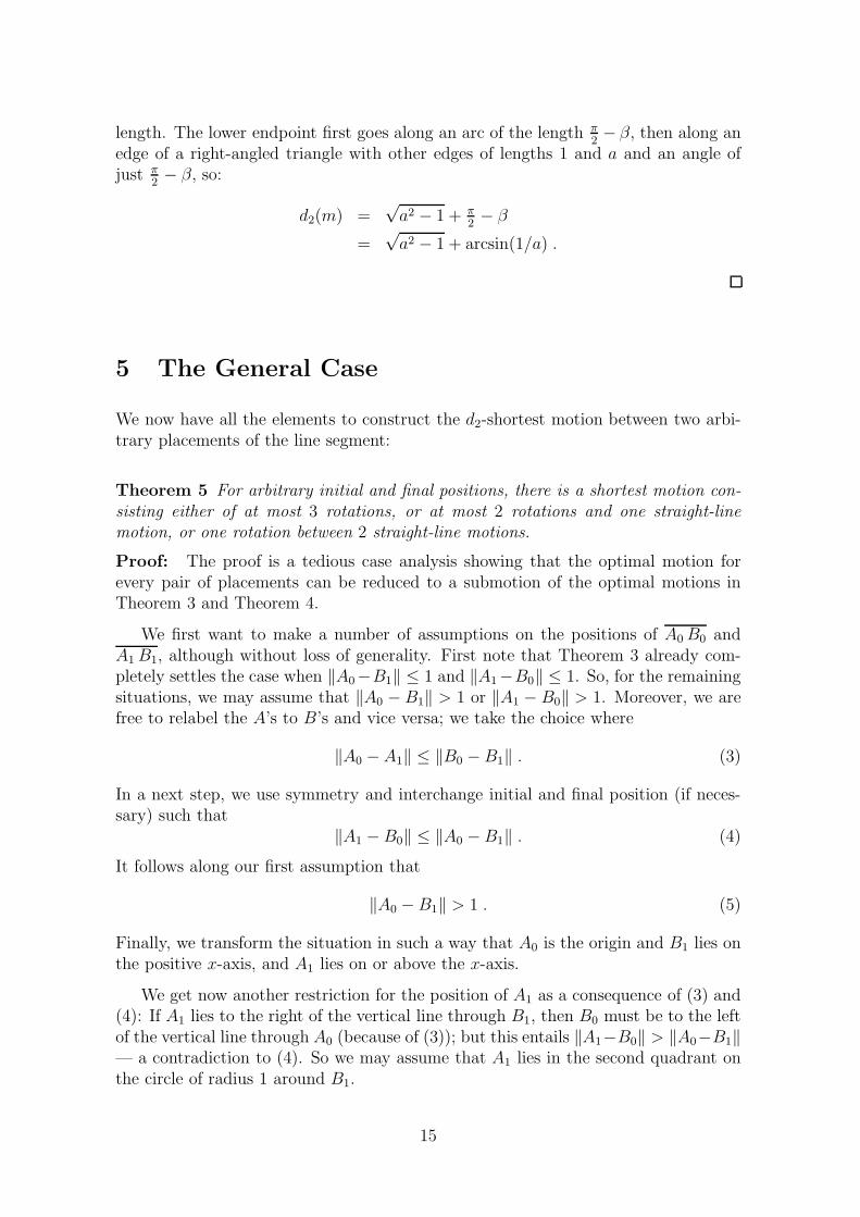
5 The General Case

We now have all the elements to construct the d2-shortest motion between two arbi-trary placements of the line segment:

Theorem 5 For arbitrary initial and final positions, there is a shortest motion con-sisting either of at most 3 rotations, or at most 2 rotations and one straight-linemotion, or one rotation between 2 straight-line motions.

Proof: The proof is a tedious case analysis showing that the optimal motion forevery pair of placements can be reduced to a submotion of the optimal motions inTheorem 3 and Theorem 4.

We first want to make a number of assumptions on the positions of A0 B0 andA1 B1, although without loss of generality. First note that Theorem 3 already com-pletely settles the case when ‖A0−B1‖ ≤ 1 and ‖A1−B0‖ ≤ 1. So, for the remainingsituations, we may assume that ‖A0 − B1‖ > 1 or ‖A1 − B0‖ > 1. Moreover, we arefree to relabel the A’s to B’s and vice versa; we take the choice where

‖A0 − A1‖ ≤ ‖B0 − B1‖ . (3)

In a next step, we use symmetry and interchange initial and final position (if neces-sary) such that

‖A1 − B0‖ ≤ ‖A0 − B1‖ . (4)

It follows along our first assumption that

‖A0 − B1‖ > 1 . (5)

Finally, we transform the situation in such a way that A0 is the origin and B1 lies onthe positive x-axis, and A1 lies on or above the x-axis.

We get now another restriction for the position of A1 as a consequence of (3) and(4): If A1 lies to the right of the vertical line through B1, then B0 must be to the leftof the vertical line through A0 (because of (3)); but this entails ‖A1−B0‖ > ‖A0−B1‖— a contradiction to (4). So we may assume that A1 lies in the second quadrant onthe circle of radius 1 around B1.

15

B1A0

P1

P2P3

Q2

Q1

p1

p2

p0 q1q0

q2

Figure 8: Partitioning for the case analysis.

Unfortunately, we have to go through a case analysis; in order to discriminate thedifferent cases we have to identify points on the circles of radius 1 around B1 and A0.Since ‖A0 − B1‖ > 1, we may speak of the tangents of the circle around B1 throughA0 (circles are always of radius 1 — from now on).

Let q1 be the point where the tangent of positive slope touches the circle aroundB1. Let q0 be the point vertically above B1 on the circle and let q2 be the pointhorizontally to the left of B1 on the circle (cf. Figure 8). We caution that Figure 8may be slightly misleading because in general, the two circles indicated could intersect.But our arguments will not hinge on their non-intersection.

We distinguish for A1 the positions Q1 between q0 and q1 (including q0) and thepositions Q2 between q1 and q2 (including q1 and q2).

Let us switch to the circle around A0. Its tangents through B1 touch in two points;let p0 be the one above the x-axis, and let p2 be the one below. Let p1 be the pointdiametrically opposite to p2. We distinguish the three intervals P1 between p0 and p1,P2 between p1 and p2, and P3 between p2 and p0 (always the second point included).Note now that if A1 ∈ Q1 and B0 ∈ P3, then

‖A0 − A1‖ > ‖A0 − q1‖ = ‖B1 − p0‖ ≥ ‖B1 − B0‖which contradicts (3).

If A1 ∈ Q1 and B0 ∈ P2, then

‖B0 − A1‖ > ‖B0 − q1‖ ≥ ‖p1 − q1‖ = ‖A0 − B1‖ ;

a contradiction to (4). We are ready to settle the first case.

Case 1 A1 ∈ Q1:We have just seen that this implies B0 ∈ P1. Then the following motion is optimal.Rotate B around A0 in clockwise direction until it reaches p0, then perform a straight-line motion between A0 p0 and q1 B1 and then rotate A around B1 clockwise until itreaches A1. It is clear from Theorem 4 that this motion m is optimal because condition(4) ensures that the angle rotated does not exceed π and m can be embedded in the

16

doubling of m∗ in Theorem 4. Moreover, unless A0 B0 and A1 B1 are antiparallel, themotion is unique.

Case 2 A1 ∈ Q2, B0 ∈ P3:This situation allows a straight-line motion.

Case 3 A1 ∈ Q2, B0 ∈ P1 ∪ P2:We need here another partitioning of P1∪P2 (see Figure 9). To this end let r and s bethe intersection points of the circle around A0 with the line through A0 perpendicularto A0 A1; r is the one above the x-axis.

P'P1

P'P2

B1A0

Q2

p2

p0 q1

q2

A1

r

s

Figure 9: Partitioning for Case 3.

We have r ∈ P1 and s ∈ P2. We denote by P ′1 the interval between p0 and r (r

included) and by P ′2 the interval between s and p2 (s and p2 included).

Case 3.1 B0 ∈ P ′1:

Rotate B clockwise around A0 until it reaches p0, then continue with a straight-linemotion from A0 p0 to A1 B1. Assume we prolongate the straight-line motion as faras possible, i.e., until the segment gets perpendicular to the line through A0 and A1.Then the segment is antiparallel to A0r, and this shows that the motion describedabove is a submotion of an optimal motion between the two antiparallel positions.

Case 3.2 B0 ∈ P ′2:

Observe first that if A1 = q1, then s = p2 and so B0 = p2. Hence, A0 B0 and A1 B1

are parallel which is an obvious case. Otherwise we suggest the following motion.Rotate B counterclockwise around A0 until it reaches p2 and then continue with astraight-line motion from A0 p2 to A1 B1. We can take over the reasoning for Case3.1 (with r replaced by s) to argue that this motion is optimal.

Note that we have not met a motion of the type “straight-line – rotation – straight-line” so far in our analysis. This will happen in the remaining cases which turn outto be somewhat more subtle.

Case 3.3 B0 ∈ (P1 ∪ P2) − (P ′1 ∪ P ′

2):Once more we transform the situation, namely in such a way that A0 and A1 lie onthe x-axis, A0 to the left of A1. Now r and s lie vertically above and below A0. That

17

is, B0 lies in the second or third quadrant around A0. From the fact that A1 ∈ Q2, italso easily follows that B1 lies in the fourth quadrant around A1.

Case 3.3.1 B0 lies in the third quadrant around A0 (Figure 10):

A0

B0b0

B1

r

s

t A1

b1

B'B1

Figure 10: Case 3.3.1.

Condition (4) implies that B0 lies already below B′1, the image of B1 reflected at

the bisector of A0 and A1. As anticipated this leads to a motion consisting of twostraight-line motions with a rotation in between. The rotation will be around A in apoint t. For the construction of t, we consider the tangents (from above) to the circlearound B1 through A0 and the tangent (from above) to the circle around B0 throughA1; let t be the intersection of these two tangents. Recall ‖A0 − B1‖ > 1 and notethat ‖A1 − B0‖ > ‖A0 − B0‖ = 1 to see that both tangents exist.

Point t lies between the vertical lines through A0 and A1. We have ‖t − B0‖ ≥ 1and ‖t−B1‖ ≥ 1 because t lies on tangents to the circles around the respective points.So, let b0 and b1 be the touching points of the tangents from below to the circle aroundt through B0 and B1. Now the suggested motion is: straight-line motion from A0 B0

to t b0; rotation around A in t from t b0 to t b1; and straight-line motion from t b1 toA1 B1. Since B0b0 is parallel to t A1, b1 B1 is parallel to A0 t, and the angle rotatedis at most π, it follows along the lines of the proof of Theorem 4 that this motion isoptimal.

Case 3.3.2 B0 lies in the second quadrant around A0 (Figure 11):

Condition (4) implies that B0 lies already above B′1, the image of B1 reflected at

the midpoint of A0 and A1. The reasoning can be taken over from Case 3.3.1 almostverbatim. In the construction of t we have to use tangents from below (instead ofabove), and for the construction of b0 and b1 we use tangents from above (instead ofbelow). For the fact that the rotated angle does not exceed π, we need once more theassumption that ‖A1 − B0‖ ≤ ‖A0 − B1‖.

This completes the proof of the main theorem.

18

b0

b1

A0

B'B1

B0

r

s

t

A1

B1

Figure 11: Case 3.3.2.

Recall Definition 6 about the nearness of two placements P, Q. In that case wehad shown that three rotations suffice to move from P to Q optimally (Theorem 3).We now conclude that this is also a necessary condition.

Corollary 4 There is a shortest motion from one placement to another consisting ofpure rotations if and only if the two placements are near to each other.

Proof: If the two placements are near, we know from Theorem 3 that there isa motion consisting of pure rotations. Conversely, suppose the two placements arenot near. Then the above proof shows that an optimal path (and this is essentiallyunique) is a submotion of the doubling of an optimal motion between two antiparallelplacements which are not near, as treated in Theorem 4. For antiparallel placements,nearness is equivalent to a midpoint distance a ≤ 1. But such a submotion always hasa portion consisting of a straight-line motion, as we see in the proof of Theorem 5.

6 Final Remarks

We introduced the distance measures d2, . . . , d∞ for line segment motions in the planeand proved some general properties of all these distance measures. We introduced theCauchy surface area theorem as a simple and effective tool for analyzing d2-optimalmotions. At present it is not clear how to extend our techniques from d2 to the othercases. However, one should be able to construct d2-shortest paths in the presence ofat least simple obstacles.

An interesting consequence of our main result is that there is always a d2-optimalmotion which is a sequence of straight-line motions and pure rotations. It is worth-while noting that we first arrived at this conclusion by studying the Euler-Lagrange

19

differential equations for optimal motions, before we discovered the present construc-tive procedure to find the optimal paths. But of course just knowing that straight-linemotions and pure rotations suffice was still very far from any constructive solution.

References

[AAGHI] T. Asano, T. Asano, L. Guibas, J. Hershberger, and H. Imai. Visibility-polygonsearch and Euclidean shortest paths. In Proceedings of the 26th IEEE Sym-posium on Foundations of Computer Science, 1985, pages 155–164.

[Bes] A. S. Besicovitch. On Kakeya’s problem and a similar one. MathematischeZeitschrift 27, 1928, pages 312–320.

[Bla] C. Blatter. Uber Kurven konstanter Breite. Elemente der Mathematik 36,1981, pages 105–115.

[Dub] V. A. Dubovitskij. Zadacha Ulama ob optimal’nom sovmeshchenii otrezkov (inRussian). USSR Academy of Sciences, Chernogolovka, Moscow, 1981. English transla-tion: The Ulam Problem of Optimal Motion of Line Segments. OptimizationSoftware, New York, 1985.

[Egg] H. G. Eggleston. Convexity. Cambridge University Press, Cambridge, 1958.

[Gol] M. Goldberg. The Minimum Path and the Minimum Motion of a Moved LineSegment. Mathematics Magazine 46, 1973, pages 31–34.

[Gur] A. B. Gurevich. The “Most Economical” Displacement of a Segment (in Rus-sian). Differentsial’nye Uravneniya 11, 1975, No. 12, pages 2134–2143. Englishtranslation: Differential Equations 11, 1976, pages 1583–1589.

[Hil] D. Hilbert. Uber das Dirichlet’sche Princip. Jahresbericht der DeutschenMathematiker-Vereinigung 8, 1900, pages 184–188.

[ORo] J. O’Rourke. Finding a shortest ladder path: a special case. IMA PreprintSeries #353, Institute for Mathematics and its Applications, University of Minnesota,1987.

[PaSi] C. H. Papadimitriou and E. B. Silverberg. Optimal Piecewise Linear Motion ofan Object Among Obstacles. Algorithmica 2, 1987, pages 523–539.

[Rin] W. Rinow. Die innere Geometrie der metrischen Raume. Volume 105 ofGrundlehren der Mathematischen Wissenschaften in Einzeldarstellungen,Springer-Verlag, Berlin, 1961.

[SchSh] J. T. Schwartz and M. Sharir. On the piano movers’ problem: I. The case ofa two-dimensional rigid polygonal body moving amidst polygonal barriers.Communications on Pure and Applied Mathematics 36, 1983, pages 345–398.

20

[Sha] M. Sharir. A note on the Papadimitriou-Silverberg algorithm for planningoptimal piecewise-linear motion of a ladder. NYU Robotics Report No. 188,1989.

[Ula] S. M. Ulam. Problems of Modern Mathematics. Science Editions, New York, 1964.Originally published as: A Collection of Mathematical Problems. IntersciencePublishers, New York, 1960.

[YaBo] I. M. Yaglom and V. G. Boltyanskiı. Convex Figures. Holt, Rinehart and Winston,New York, 1961.

[Yap] C. K. Yap. Algorithmic Motion Planning. In J. T. Schwartz and C. K. Yap, editors,Advances in robotics: algorithmic and geometric issue (Volume 1), LawrenceErlbaum Associates, Hillsdale, New Jersey, 1987.

21