MATH 2070–03 Differential Equations Dr. Lori Alvin

Section 6.1 - 6.2 Notes Laplace Transforms

Name:

A short table of Laplace transforms appears on the last page. We begin by reviewing somebasic calculus results before introducing the Laplace Transform.

Review: Limits of exponential functions

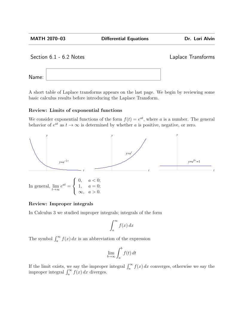
We consider exponential functions of the form f(t) = eat, where a is a number. The generalbehavior of eat as t→∞ is determined by whether a is positive, negative, or zero.

t

y

y=e-2 t

t

y

y=et

t

y

y=e0 t=1

In general, limt→∞

eat =

0, a < 0;1, a = 0;∞, a > 0.

Review: Improper integrals

In Calculus 3 we studied improper integrals; integrals of the form∫ ∞a

f(x) dx

The symbol∫∞af(x) dx is an abbreviation of the expression

limb→∞

∫ b

a

f(t) dt

If the limit exists, we say the improper integral∫∞af(x) dx converges, otherwise we say the

improper integral∫∞af(x) dx diverges.

Exercise 1. Decide whether the following improper integrals converge or diverge. For thosethat converge, compute their values.(a)

∫∞0e−4x dx

(b)∫∞0te−3t dt

(c)∫∞0et/2 dt

(d)∫∞0

1x lnx

dx

Exercise 2. For which values of s does the integral∫∞0e−st dt converge?

The Laplace Transform

The Laplace Transform is another way of writing a function.Usually when we talk about a function, we talk about its values. We evaluate the function

by substituting numbers into the formula. For example, we evaluate f(x) =1

4 + x2at x = 3

by substituting 3 into the formula: f(3) =1

4 + 32=

1

13. Two functions f(x) and g(x) are

the same if every possible evaluation produces the same result, that is if f(a) and g(a) arethe same for every a in the domains of f and g.There are other ways to “test” functions, that is, to make them produce numbers. Oneway is to multiply them with other functions and then integrate. We can think of this as ageneralization of evaluation.Given functions f and g defined on the interval [0,∞), we can integrate f against g, thatis, compute ∫ ∞

0

f(t)g(t) dt

For many choices of g, the result will be a number. We will mainly be interested in theresults of integrating f against exponential functions, such as e−4t:∫ ∞

0

f(t)e−4t dt

or, more generally, ∫ ∞0

f(t)e−st dt.

For different values of s, the result will be a number, depending on s.

Definition The Laplace transform function Y of the function y is defined by

Y (s) =

∫ ∞0

y(t)e−st dt

for all numbers s for which the integral converges.

Page 2

Example. Compute the Laplace transform of y(t) = e5t and state its domain.

We can think of the value of Y (s) as measuring how closely the function y(t) resembles thefunction est: when Y (s) is very large, the function y(t) closely resembles est, and when Y (s)is small, the function y(t) is very different from est.

Page 3

Notation.

If y(t) is a function, we may write L [y(t))] for its laplace transform. So

L [e5t] =1

s− 5for s > 5

The Laplace Transform and Derivatives

The reason for even considering the Laplace transform is because of the nice relationshipbetween the Laplace transform of a function y(t) and the Laplace transform of its derivativedydt

.

Laplace Transform of Derivatives Given a function y(t) with Laplace transform L [y],

the Laplace transform ofdy

dtis

L[dydt

]= sL [y]− y(0).

This is a consequence of the definition of the Laplace transform and integration by parts:

L[dydt

]=

∫ ∞0

(dydt

)e−st dt.

Page 4

Exercise 3. Verify that the formula L[dydt

]= sL [y]− y(0) holds for the function y(t) = t.

That is, compute L [t], compute L [1], and show that L [1] = sL [t]− 0.

Linearity

The following standard properties of integration

∫f(t)+g(t) dt =

∫f(t) dt+

∫g(t) dt and∫

cf(t) dt = c

∫f(t) dt lead to the corresponding properties for the Laplace transform:

L [f + g] = L [f ] + L [g]

[cf ] = c[f ].

Page 5

General Procedure for Solving a First-order Linear equation using Laplace trans-forms

Given an initial value problem

dy

dt= a(t)y + b(t), y(0) = y0

(Usually a(t) is a constant.)

1. Compute the Laplace transform of both sides, using the identity L[dydt

]= sL [y]− y(0)

on the left-hand side.

2. Solve for L [y]: you will have a solution of the form L [y] = g(s).

3. Break g(s) down as a sum of simple functions (hopefully the ones that appear in the tableof Laplace transforms on page 626). Use partial fractions if necessary.

4. Compute the inverse Laplace transform of g(s): your answer will be

y(t) = L −1[g(s)]

Example. Solve

dy

dt= y − t y(0) = 1

using Laplace transforms.

Page 6

Discontinuous functions in differential equations

The Heaviside function

ua(t) =

{0, if t < a;1, if t ≥ a.

The Laplace transform of ua(t):

L [ua] =e−as

s

The Heaviside function is useful in modeling physical situations where something changesabruptly at a certain time.

Example. Solve the initial value problem

dy

dt= −y + 4u2(t); y(0) = 3

Page 7

.

Page 8

.

Remarks. The answer produced by Solution (B) is actually the same as the answer producedby Solution (A). You can check that they are the same by simplifying the answer from (B):

4u2(t)(1− e−(t−2)) + 3e−t =

3e−t, if t < 2;

4(1− e−(t−2)) + 3e−t, if t ≥ 2.

and the second part simplifies as (3− 4e−2)et + 4.

Page 9

Example. Solve the initial-value problemdy

dt= 2y+e−3t, y(0) = 1 using Laplace transforms.

Page 10

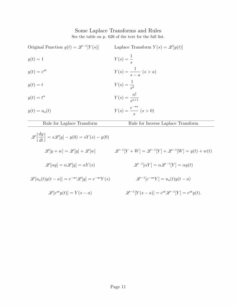
Some Laplace Transforms and RulesSee the table on p. 626 of the text for the full list.

Original Function y(t) = L −1[Y (s)] Laplace Transform Y (s) = L [y(t)]

y(t) = 1 Y (s) =1

s

y(t) = eat Y (s) =1

s− a(s > a)

y(t) = t Y (s) =1

s2

y(t) = tn Y (s) =n!

sn+1

y(t) = ua(t) Y (s) =e−as

s(s > 0)

Rule for Laplace Transform Rule for Inverse Laplace Transform

L[dydt

]= sL [y]− y(0) = sY (s)− y(0)

L [y + w] = L [y] + L [w] L −1[Y +W ] = L −1[Y ] + L −1[W ] = y(t) + w(t)

L [αy] = αL [y] = αY (s) L −1[αY ] = αL −1[Y ] = αy(t)

L [ua(t)y(t− a)] = e−asL [y] = e−asY (s) L −1[e−asY ] = ua(t)y(t− a)

L [eaty(t)] = Y (s− a) L −1[Y (s− a)] = eatL −1[Y ] = eaty(t).

Page 11