Download pdf - Rigid Body Mechanics

Rigid Body Mechanics 2

In which we find that a rigid body has six degrees of freedom, learn how to describe the orientation of

a rigid body in terms of Euler angles, define inertial and body coordinates and find the Euler-Lagrange

equations for a single rigid body. . .

Kinematics

I will develop the idea of a rigid body using what we have already from systems of particles. A rigid

body can be viewed as a system of constrained particles. I will need to discuss degrees of freedom and

constraints as part of this process. This will be useful as an introduction to a fuller discussion of

constraints in Chap. 3.

The number of degrees of freedom of a system is the minimum number of variables needed to

specify the system. A particle has three degrees of freedom: translation in three independent

directions (typically with respect to a Cartesian axis, but this is not necessary). Two particles have

six degrees of freedom – three each – but were they rigidly attached, the total number of degrees of

freedom would be reduced to five. The argument is simple. Denote the positions of the two particles

by r1 and r2 respectively. If the particles are rigidly attached the distance between them is fixed. We

say that there is a constraint enforcing this:

r1 � r2ð Þ � r1 � r2ð Þ ¼ d2 (2.1)

where d denotes the distance between the two particles. I have written the constraint in terms of the

coordinates of the two masses. This is the definition of a holonomic constraint. (I will address

nonholonomic constraints, which cannot be so written, in Chap. 3.) In principle, we can use the

constraint to eliminate one of the six coordinates, but this is an unwieldy task (try it!), and it is easier

to parameterize the constraint1. One useful way to do this is to write

x2 ¼ x1 þ d cos α sin β; y2 ¼ y1 þ d sin α sin β; z2 ¼ z1 þ d cos β (2.2)

1 I will address another alternative in Chap. 3.

R.F. Gans, Engineering Dynamics: From the Lagrangian to Simulation,DOI 10.1007/978-1-4614-3930-1_2, # Springer Science+Business Media New York 2013

31

http://dx.doi.org/10.1007/978-1-4614-3930-1_3

http://dx.doi.org/10.1007/978-1-4614-3930-1_3

http://dx.doi.org/10.1007/978-1-4614-3930-1_3

(The reader can verify that this satisfies Eq. 2.1). The five degrees of freedom are then described by

the three components of r1 and the two angles. (The angles will look familiar: α corresponds to the

usual spherical coordinate angle ϕ and β to θ. I use α and β because I want to reserve ϕ and θ [and ψ]for Euler angles). The parameterization says that r2 lies on a sphere surrounding r1.

Adding a third point leads us directly to the rigid body. The thought process is as follows. Suppose

the third point to be at r3. Denote the fixed distances between the points by d12, d13, d23, respectively.The third point must lie on a sphere of radius d13 from r1 and a sphere of radius d23 from r2. Two

spheres intersect in a circle, so the third point can be anywhere on that circle. This means that it has

but one degree of freedom, so that the system of three rigidly attached particles has six degrees of

freedom, the five associated with the first two rigidly-connected particles, plus the one additional

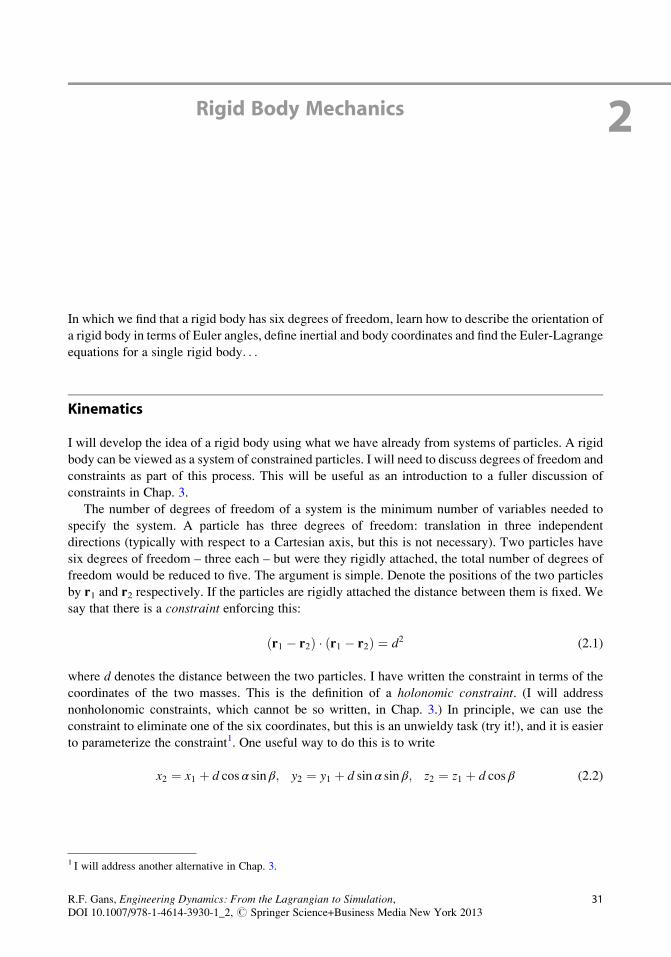
degree of freedom, the location of the third point on the circle of intersection. Figure 2.1 shows the

original two points and the two spheres.

Each additional particle must lie at the intersection of at least three spheres. Three spheres intersect

at a point (if at all), so additional particles add no additional degrees of freedom. The number of

degrees of freedom of a single rigid body is six.

A Geometrical Digression onto a Plane

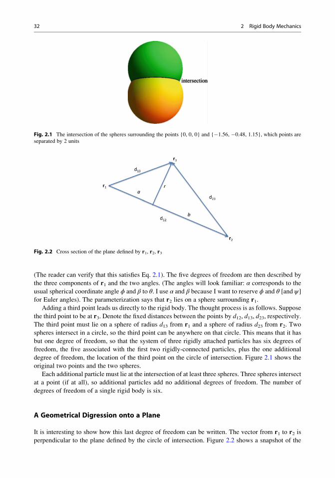
It is interesting to show how this last degree of freedom can be written. The vector from r1 to r2 is

perpendicular to the plane defined by the circle of intersection. Figure 2.2 shows a snapshot of the

Fig. 2.1 The intersection of the spheres surrounding the points {0, 0, 0} and {�1.56, �0.48, 1.15}, which points are

separated by 2 units

Fig. 2.2 Cross section of the plane defined by r1, r2, r3

32 2 Rigid Body Mechanics

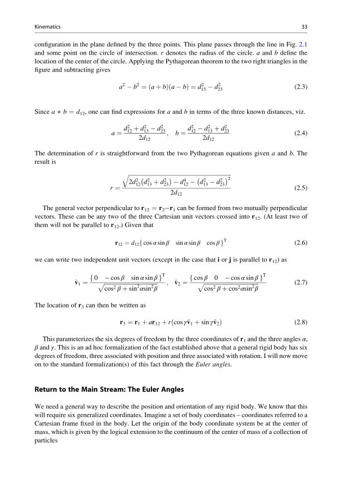
configuration in the plane defined by the three points. This plane passes through the line in Fig. 2.1

and some point on the circle of intersection. r denotes the radius of the circle. a and b define the

location of the center of the circle. Applying the Pythagorean theorem to the two right triangles in the

figure and subtracting gives

a2 � b2 ¼ aþ bð Þ a� bð Þ ¼ d213 � d223 (2.3)

Since a + b ¼ d12, one can find expressions for a and b in terms of the three known distances, viz.

a ¼ d212 þ d213 � d2232d12

; b ¼ d212 � d213 þ d2232d12

(2.4)

The determination of r is straightforward from the two Pythagorean equations given a and b. Theresult is

r ¼ffiffiffiffiffiffiffiffiffiffiffiffiffiffiffiffiffiffiffiffiffiffiffiffiffiffiffiffiffiffiffiffiffiffiffiffiffiffiffiffiffiffiffiffiffiffiffiffiffiffiffiffiffiffiffiffiffiffiffiffiffiffiffiffiffiffiffiffiffiffiffiffiffi2d212 d213 þ d223

� �� d412 � d213 � d223� �2q

2d12(2.5)

The general vector perpendicular to r12 ¼ r2�r1 can be formed from two mutually perpendicular

vectors. These can be any two of the three Cartesian unit vectors crossed into r12. (At least two of

them will not be parallel to r12.) Given that

r12 ¼ d12 cos α sin β sin α sin β cos βf gT (2.6)

we can write two independent unit vectors (except in the case that i or j is parallel to r12) as

v̂1 ¼ 0 � cos β sin α sin βf gTffiffiffiffiffiffiffiffiffiffiffiffiffiffiffiffiffiffiffiffiffiffiffiffiffiffiffiffiffiffiffiffiffiffiffiffiffifficos2 β þ sin2αsin2β

p ; v̂2 ¼ cos β 0 � cos α sin βf gTffiffiffiffiffiffiffiffiffiffiffiffiffiffiffiffiffiffiffiffiffiffiffiffiffiffiffiffiffiffiffiffiffiffiffiffiffiffifficos2 β þ cos2αsin2β

p (2.7)

The location of r3 can then be written as

r3 ¼ r1 þ ar12 þ r cos γv̂1 þ sin γv̂2ð Þ (2.8)

This parameterizes the six degrees of freedom by the three coordinates of r1 and the three angles α,β and γ. This is an ad hoc formalization of the fact established above that a general rigid body has six

degrees of freedom, three associated with position and three associated with rotation. I will now move

on to the standard formalization(s) of this fact through the Euler angles.

Return to the Main Stream: The Euler Angles

We need a general way to describe the position and orientation of any rigid body. We know that this

will require six generalized coordinates. Imagine a set of body coordinates – coordinates referred to a

Cartesian frame fixed in the body. Let the origin of the body coordinate system be at the center of

mass, which is given by the logical extension to the continuum of the center of mass of a collection of

particles

Kinematics 33

rCM ¼

Ðvolume

ρrdV

m(2.9)

The first three degrees of freedom are the inertial coordinates of the center of mass; the other three

come from the orientation of the body, the angular relations between the body axes and the inertial

axes. These six variables uniquely define the position of a body. I will sometimes refer to this as the

posture of the body. I will replace the ad hoc description above with the standard description in terms

of the Euler angles, which I will now develop.

Denote the body Cartesian coordinates by (X, Y, Z) and denote the corresponding unit vectors by

I, J,K. Denote the unit vectors for the inertial (x, y, z) system by i, j, k. Any vector can be defined with

respect to either coordinate system. Denote the inertial description by v and the body description by

V. The connection between these two can be defined using the basis vectors. We’ll have

v ¼ vxiþ vyjþ vzk ¼ V ¼ VXIþ VYJþ VZK

The inertial components in terms of the body components are

vx ¼ VXi � Iþ VY i � Jþ VZi �Kvy ¼ VXj � Iþ VYj � Jþ VZj �Kvz ¼ VXk � Iþ VYk � Jþ VZk �K

which can be written in matrix form as

vx

vy

vz

8><>:

9>=>; ¼

i � I i � J i �Kj � I j � J j �Kk � I k � J k �K

8><>:

9>=>;

VX

VY

VZ

8><>:

9>=>; (2.10)

The body components can be written in terms of the inertial coordinates by a similar process. The

matrix form is

VX

VY

VZ

8><>:

9>=>; ¼

i � I j � I k � Ii � J j � J k � Ji �K j �K k �K

8><>:

9>=>;

vx

vy

vz

8><>:

9>=>; (2.11)

The two matrices are both mutual transposes and mutual inverses. All that we need to complete the

process is to find the dot products. We can do this formally using the Euler angles, but it will be

helpful to go through the process in a less formal, more ad hoc process. The manipulation of vectors

and angles is a remarkably important part of three dimensional rigid body mechanics, so more than

one exposition is not amiss. We need a relationship between the inertial basis vectors and the body

basis vectors, and we can develop that by supposing that the two systems start out coincident and that

we then rotate the body basis vectors with respect to the inertial frame. There are many ways to do

this. I will use the common Euler angles in an intuitive method, which I will formalize shortly. The

idea is to rotate the body frame about three of its own axes successively by the angles ϕ, θ, and ψ . Thedifference between this and the formalism is that I take an inertial point of view for this discussion.

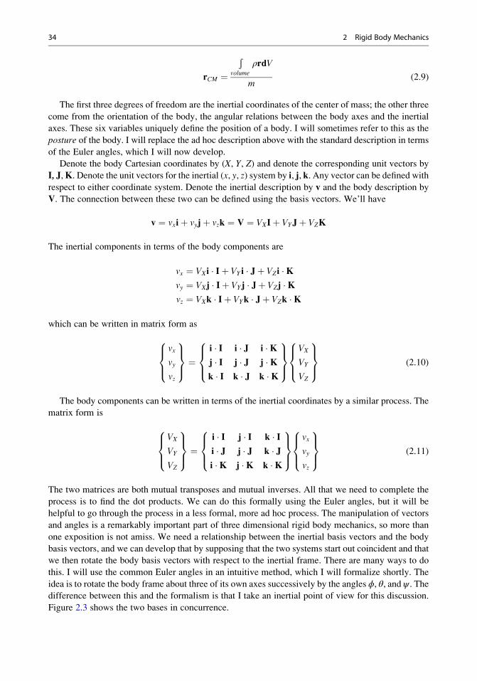
Figure 2.3 shows the two bases in concurrence.


The standard Euler rotations start by rotating the body system counterclockwise about itsK axis by

an angle ϕ. The vectors I and J change while K remains fixed. We can write the vectors after the first

rotation in terms of their original positions

I1 ¼ cosϕI0 þ sinϕJ0; J1 ¼ � sinϕI0 þ cosϕJ0; K1 ¼ K0 (2.12a)

where the subscript denotes the number of rotations. Figure 2.4 shows the system after this rotation.

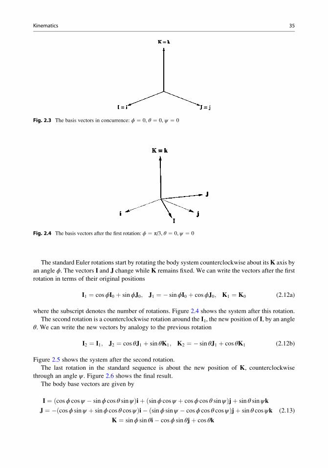
The second rotation is a counterclockwise rotation around the I1, the new position of I, by an angle

θ. We can write the new vectors by analogy to the previous rotation

I2 ¼ I1; J2 ¼ cos θJ1 þ sin θK1; K2 ¼ � sin θJ1 þ cos θK1 (2.12b)

Figure 2.5 shows the system after the second rotation.

The last rotation in the standard sequence is about the new position of K, counterclockwise

through an angle ψ . Figure 2.6 shows the final result.

The body base vectors are given by

I ¼ cosϕ cosψ � sinϕ cos θ sinψð Þiþ sinϕ cosψ þ cosϕ cos θ sinψð Þjþ sin θ sinψk

J ¼ � cosϕ sinψ þ sinϕ cos θ cosψð Þi� sinϕ sinψ � cosϕ cos θ cosψð Þjþ sin θ cosψk

K ¼ sinϕ sin θi� cosϕ sin θjþ cos θk

(2.13)

Fig. 2.3 The basis vectors in concurrence: ϕ ¼ 0, θ ¼ 0, ψ ¼ 0

Fig. 2.4 The basis vectors after the first rotation: ϕ ¼ π/3, θ ¼ 0, ψ ¼ 0

Kinematics 35

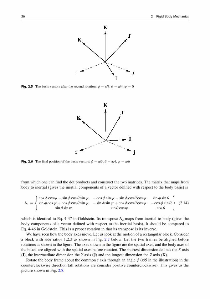
from which one can find the dot products and construct the two matrices. The matrix that maps from

body to inertial (gives the inertial components of a vector defined with respect to the body basis) is

A1 ¼cosϕ cosψ � sinϕ cos θ sinψ � cosϕ sinψ � sinϕ cos θ cos ψ sinϕ sin θsinϕ cosψ þ cosϕ cos θ sinψ � sinϕ sinψ þ cosϕ cos θ cos ψ � cosϕ sin θ

sin θ sinψ sin θ cosψ cos θ

8<:

9=; (2.14)

which is identical to Eq. 4-47 in Goldstein. Its transpose A2 maps from inertial to body (gives the

body components of a vector defined with respect to the inertial basis). It should be compared to

Eq. 4-46 in Goldstein. This is a proper rotation in that its transpose is its inverse.

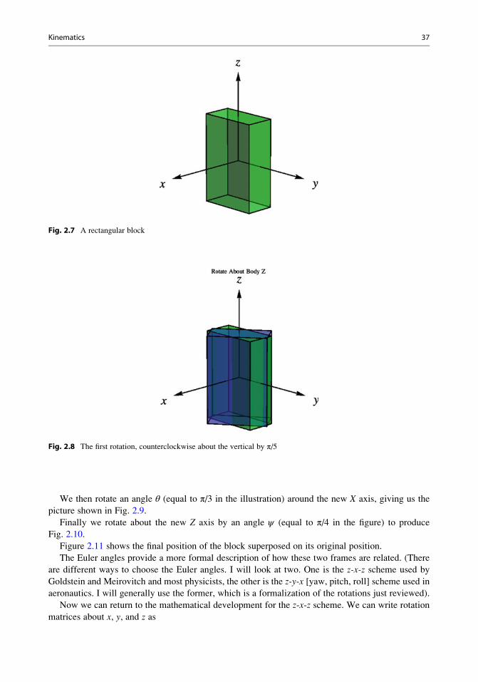
We have seen how the body axes move. Let us look at the motion of a rectangular block. Consider

a block with side ratios 1:2:3 as shown in Fig. 2.7 below. Let the two frames be aligned before

rotations as shown in the figure. The axes shown in the figure are the spatial axes, and the body axes of

the block are aligned with the spatial axes before rotation. The shortest dimension defines the X axis

(I), the intermediate dimension the Y axis (J) and the longest dimension the Z axis (K).

Rotate the body frame about the common z axis through an angle ϕ (π/5 in the illustration) in the

counterclockwise direction (all rotations are consider positive counterclockwise). This gives us the

picture shown in Fig. 2.8.

Fig. 2.5 The basis vectors after the second rotation: ϕ ¼ π/3, θ ¼ π/4, ψ ¼ 0

Fig. 2.6 The final position of the basis vectors: ϕ ¼ π/3, θ ¼ π/4, ψ ¼ π/6


We then rotate an angle θ (equal to π/3 in the illustration) around the new X axis, giving us the

picture shown in Fig. 2.9.

Finally we rotate about the new Z axis by an angle ψ (equal to π/4 in the figure) to produce

Fig. 2.10.

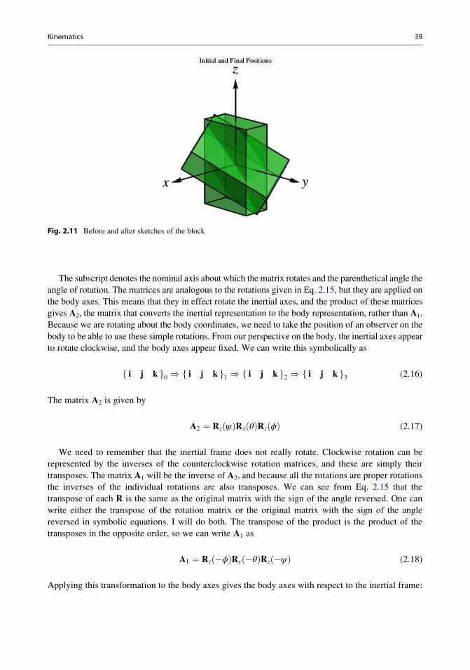
Figure 2.11 shows the final position of the block superposed on its original position.

The Euler angles provide a more formal description of how these two frames are related. (There

are different ways to choose the Euler angles. I will look at two. One is the z-x-z scheme used by

Goldstein and Meirovitch and most physicists, the other is the z-y-x [yaw, pitch, roll] scheme used in

aeronautics. I will generally use the former, which is a formalization of the rotations just reviewed).

Now we can return to the mathematical development for the z-x-z scheme. We can write rotation

matrices about x, y, and z as

Fig. 2.7 A rectangular block

Fig. 2.8 The first rotation, counterclockwise about the vertical by π/5

Kinematics 37

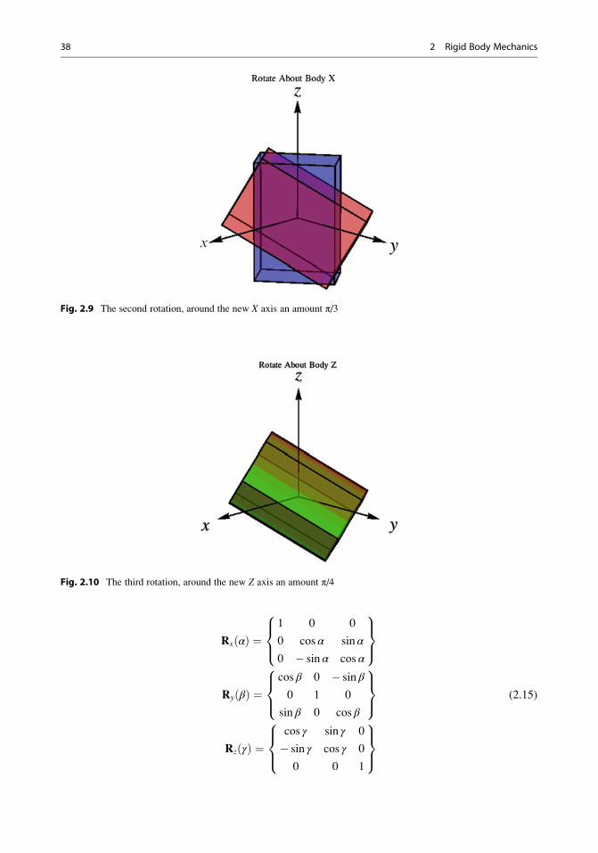
Rx αð Þ ¼1 0 0

0 cos α sin α

0 � sin α cos α

8><>:

9>=>;

Ry βð Þ ¼cos β 0 � sin β

0 1 0

sin β 0 cos β

8><>:

9>=>;

Rz γð Þ ¼cos γ sin γ 0

� sin γ cos γ 0

0 0 1

8><>:

9>=>;

(2.15)

Fig. 2.9 The second rotation, around the new X axis an amount π/3

Fig. 2.10 The third rotation, around the new Z axis an amount π/4


The subscript denotes the nominal axis about which the matrix rotates and the parenthetical angle the

angle of rotation. The matrices are analogous to the rotations given in Eq. 2.15, but they are applied on

the body axes. This means that they in effect rotate the inertial axes, and the product of these matrices

gives A2, the matrix that converts the inertial representation to the body representation, rather than A1.

Because we are rotating about the body coordinates, we need to take the position of an observer on the

body to be able to use these simple rotations. From our perspective on the body, the inertial axes appear

to rotate clockwise, and the body axes appear fixed. We can write this symbolically as

i j kf g0 ) i j kf g1 ) i j kf g2 ) i j kf g3 (2.16)

The matrix A2 is given by

A2 ¼ Rz ψð ÞRx θð ÞRz ϕð Þ (2.17)

We need to remember that the inertial frame does not really rotate. Clockwise rotation can be

represented by the inverses of the counterclockwise rotation matrices, and these are simply their

transposes. The matrix A1 will be the inverse of A2, and because all the rotations are proper rotations

the inverses of the individual rotations are also transposes. We can see from Eq. 2.15 that the

transpose of each R is the same as the original matrix with the sign of the angle reversed. One can

write either the transpose of the rotation matrix or the original matrix with the sign of the angle

reversed in symbolic equations. I will do both. The transpose of the product is the product of the

transposes in the opposite order, so we can write A1 as

A1 ¼ Rz �ϕð ÞRx �θð ÞRz �ψð Þ (2.18)

Applying this transformation to the body axes gives the body axes with respect to the inertial frame:

Fig. 2.11 Before and after sketches of the block

Kinematics 39

I ¼1

0

0

8><>:

9>=>; )

cosϕ cosψ � cos θ sinϕ sinψ

cosψ sinϕþ cos θ cosϕ sinψ

sin θ sinψ

8><>:

9>=>;

J ¼0

1

0

8><>:

9>=>; )

� cosϕ sinψ � cos θ sinϕ cosψ

� sinψ sinϕþ cos θ cosϕ cosψ

sin θ cosψ

8><>:

9>=>;

K ¼0

0

1

8><>:

9>=>; )

sin θ sinϕ

� cosϕ sin θ

cos θ

8><>:

9>=>;

(2.19)

I leave it to the reader to verify these.

We can summarize these rules. Suppose that we start with the body basis vectors in concurrence

with the inertial basis vectors, and rotate about a succession of body axes by a succession of angles α1,α2, etc. The two transformation matrices are

A1 ¼ R1 �α1ð ÞR2 �α2ð Þ � � �RN �αNð ÞA2 ¼ RN αNð Þ � � �R2 α2ð ÞR1 α1ð Þ (2.20)

We will have occasion later in the text to use more than three rotations. This will arise when we

have multilink mechanisms in which two links share all three Euler angles, but one of the links rotates

with respect to the rest of the system in yet another direction. Equation 2.20 will be very useful in such

cases.

It is essential to note that these finite rotations do not commute. The rotation Rx(π/2).Rz(π/2)carries the body frame I, J, K to j, k, i, respectively, while the rotation Rz(π/2). Rx(π/2) carries thesame set to –k, i, �j.

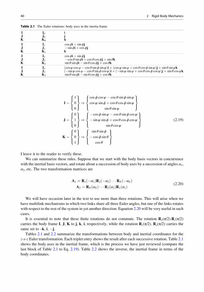
Tables 2.1 and 2.2 summarize the transformations between body and inertial coordinates for the

z-x-z Euler transformation. Each triplet entry shows the result after each successive rotation. Table 2.1

shows the body axes in the inertial frame, which is the process we have just reviewed (compare the

last block of Table 2.1 to Eq. 2.19). Table 2.2 shows the inverse, the inertial frame in terms of the

body coordinates.

Table 2.1 The Euler rotations: body axes in the inertia frame

I I0 iJ J0 jK K0 k

I I1 cosϕiþ sinϕjJ J1 �sinϕiþ cosϕjK K1 k

I I2 cosϕiþ sinϕjJ J2 �cos θ sinϕiþ cos θ cosϕjþ sin θkK K2 sin θ sinϕi� sin θ cosϕjþ cos θk

I I3 cosψ cosφ� cos θ sinϕ sinψð Þiþ cosψ sinφþ cos θ cosϕ sinψð Þjþ sin θ sinψkJ J3 �sinψ cosφ� cos θ sinϕ cosψð Þiþ �sinψ sinφþ cos θ cosϕ cosψð Þjþ sin θ cosψkK K3 sin θ sinϕi� sin θ cosϕjþ cos θk


Placing Axes

The aim of the text is to develop methods for analyzing mechanisms by building mathematical

models of them. Mechanisms are assemblies of links. The links are connected at specified locations,

and generally one body axis is aligned with some direction, either in space or on another link.

Specifying the direction of a body axis still leaves one degree of freedom – rotation about this axis.

Thus we need a method to align a body axis with an arbitrary direction and allow rotation of the body

about that axis all in the context of the Euler angles.

It takes two angles to specify a direction in space. I will use the longitude and the colatitude, which

I will denote here by α and β respectively. The unit vector in that direction is then

V ¼cos α sin βsin α sin βcos β

8<:

9=;

We can always convert an arbitrary vector given in component form to a unit vector defined by α and

β. Denote the vector by v and let it have components v1, v2, v3. Its unit vector equivalent is

v̂ ¼v1ffiffiffiffiffiffiffiffiffiffiffiffiffiffiffiffiffiffiffiffiffiffiffiffiffiffiffiffiffiffiffiffiffiffiffiffiffiffiffiffiffi

v1ð Þ2 þ v2ð Þ2 þ v3ð Þ2q v2ffiffiffiffiffiffiffiffiffiffiffiffiffiffiffiffiffiffiffiffiffiffiffiffiffiffiffiffiffiffiffiffiffiffiffiffiffiffiffiffiffi

v1ð Þ2 þ v2ð Þ2 þ v3ð Þ2q v3ffiffiffiffiffiffiffiffiffiffiffiffiffiffiffiffiffiffiffiffiffiffiffiffiffiffiffiffiffiffiffiffiffiffiffiffiffiffiffiffiffi

v1ð Þ2 þ v2ð Þ2 þ v3ð Þ2q( )T

The angle β lies between 0 and π, so the cosine is unambiguously positive and we can write

β ¼ cos�1v̂3. The angle α can take any value from 0 to 2π, so one has to be careful in taking the

inverse tangent to identify the proper quadrant. Fortunately most software now has an arctangent

function that does this automatically, so we can write

α ¼ tan�1 v2

v1

� �

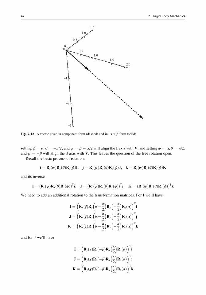
without fear of difficulty. Figure 2.12 shows the vector {2, 3/2, �3}T and its unit vector in terms of a

(¼ 0.6435) and b (¼ 2.4469). They are clearly aligned.

It should be clear that we can align the body K axis with V by simply letting ϕ ¼ α + π/2 and

θ ¼ β, leaving the third Euler angle ψ for rotation about K. Aligning the I and J axes with V is

straightforward, but adding the rotation about those axes is not. I leave it to the reader to verify that

Table 2.2 The Euler rotations: inertial axes in the body frame

i i0 Ij j0 Jk k0 K

i i1 cosϕI� sinϕJj j1 sinϕIþ cosϕJk k1 K

i i2 cosϕI� cos θ sinϕJþ sin θ sinϕKj j2 sinϕIþ cos θ cosϕJ� sin θ cosϕKk k2 sin θJþ cos θK

i i3 cosψ cosφ� cos θ sinϕ sinψð ÞIþ �cos θ cosψ sinφ� cosϕ sinψð ÞJþ sin θ sinϕKj j3 cosψ sinφþ cos θ cosϕ sinψð ÞIþ �sinψ sinφþ cos θ cosϕ cosψð ÞJ� sin θ cosϕKk k3 sin θ sinψIþ sin θ cosψJþ cos θK

Kinematics 41

setting ϕ ¼ α, θ ¼ �π/2, and ψ ¼ β � π/2 will align the I axis with V, and setting ϕ ¼ α, θ ¼ π/2,and ψ ¼ �β will align the J axis with V. This leaves the question of the free rotation open.

Recall the basic process of rotation:

i ¼ Rz ψð ÞRx θð ÞRz ϕð ÞI; j ¼ Rz ψð ÞRx θð ÞRz ϕð ÞJ; k ¼ Rz ψð ÞRx θð ÞRz ϕð ÞK

and its inverse

I ¼ Rz ψð ÞRx θð ÞRz ϕð Þð ÞTi; J ¼ Rz ψð ÞRx θð ÞRz ϕð Þð ÞTj; K ¼ Rz ψð ÞRx θð ÞRz ϕð Þð ÞTk

We need to add an additional rotation to the transformation matrices. For I we’ll have

I ¼ Rx ξð ÞRz β � π

2

� �Rx � π

2

� �Rz αð Þ

� �T

i

J ¼ Rx ξð ÞRz β � π

2

� �Rx � π

2

� �Rz αð Þ

� �T

j

K ¼ Rx ξð ÞRz β � π

2

� �Rx � π

2

� �Rz αð Þ

� �T

k

and for J we’ll have

I ¼ Ry χð ÞRz �βð ÞRxπ

2

� �Rz αð Þ

� �T

i

J ¼ Ry χð ÞRz �βð ÞRxπ

2

� �Rz αð Þ

� �T

j

K ¼ Ry χð ÞRz �βð ÞRxπ

2

� �Rz αð Þ

� �T

k

−3

−2

−1

00.0

0.5

0.5

1.0

1.0

1.5

2.01.5

Fig. 2.12 A vector given in component form (dashed) and in its α, β form (solid)


The angle ψ is a fixed constant for both of these transformations, but there is a new angle expressing

the free rotation about the axis in question. We can write these out to see how this goes. For I

we have

I ¼cos α sin β

sin α sin β

cos β

8><>:

9>=>;; J ¼

� sin α sin ξþ cos α cos β cos ξ

cos α sin ξ sin α cos β cos ξ

� sin β cos ξ

8><>:

9>=>;;

K ¼� sin α cos ξ� cos α cos β sin ξ

cos α cos ξ� sin α cos β sin ξ

sin β sin ξ

8><>:

9>=>;

and for J we have

I ¼� sin α sin χ þ cos α cos β cos χ

cos α sin χ þ sin α cos β cos χ

� sin β cos χ

8><>:

9>=>;; J ¼

cos α sin β

sin α sin β

cos β

8><>:

9>=>;;

K ¼sin α cos χ þ cos α cos β sin χ

� cos α cos χ þ sin α cos β sin χ

� sin β sin χ

8><>:

9>=>;

−0.5

0.5

z

x

y

0.5 0.5

I

K

J

0.00.00.0

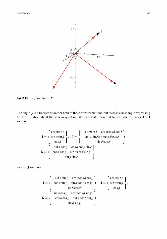
Fig. 2.13 Body axes for I ~ V

Kinematics 43

Figures 2.13, 2.14 and 2.15 show the axis alignment for I ~ V, J ~ V and K ~ V, respectively.The thin line represents 1.2 V, the extension to allow one to see it. The thick lines are the body axes as

labeled. The angles α ¼ 3π/4 and β ¼ π/3, and the final rotation angles ξ ¼ π/4, χ ¼ π/2, ψ ¼ πrespectively.

The Rotation Vector

The instantaneous rotation vector can be expressed in terms of the derivatives of the Euler angles.

The rotations represented by each Euler angle do not form a simple orthogonal triad, so we need to be

careful. In order to make use of the expressions for angular momentum and kinetic energy in terms of

0.00.00.0

0.2

0.4

0.6

0.8

0.50.5

−0.5

I

K

J

y

x

Fig. 2.14 Body axes for J ~ V

0.00.00.0

0.20.40.60.8 0.5

0.5

−0.5

−0.5I

K

J

y

x

z

Fig. 2.15 Body axes for K ~ V


principal axes, it is most useful to express the rotation vector in terms of the body axes. _ϕ represents

rotation about the inertial z axis, so it can be represented in body coordinates by _ϕ times k in body

coordinates, the last line of Table 2.2. _ψ represents rotation about the K axis and so needs no

transformation. _θ represents rotation about the intermediate axis I1. This is given in inertial

coordinates by the fourth line of Table 2.1. Replacing i and j by their expressions in terms of I, J,

K from the last block of Table 2.2 gives _θ cosψI� sinψJð Þ. We can gather up all the components of

Ω, the rotation vector in terms of the body axes, in terms of the Euler angles and their derivatives:

Ω ¼ _ϕ sin θ sinψ þ _θ cosψ� �

Iþ _ϕ sin θ cosψ � _θ sinψ� �

Jþ _ϕ cos θ þ _ψ� �

K (2.21a)

This can be converted to inertial coordinates and the result, which will be useful later, is

ω ¼ _ψ sin θ sinϕþ _θ cosϕ� �

iþ � _ψ cosϕ sin θ þ _θ sinϕ� �

jþ _ψ cos θ þ _ϕ� �

k (2.21b)

We can summarize some useful facts about the Euler angles. Rotation about k is given by ϕ.Rotation about K is given by ψ . The angle θ is may be deduced from the dot product k.K ¼ cosθ.When k and K are coincident we use ψ to denote the rotation and take ϕ ¼ 0 ¼ θ.2 These

conventions will be very useful in the study of robot motion. I will call the set of Euler angles the

Euler triad. It will also be useful to have a notation for the Euler triad. I will useΦ ¼ {ϕ, θ, ψ}, and Iwill adopt the convention that {0, 0, 0} corresponds to I ¼ i, J ¼ j, K ¼ k. I leave it to the reader to

work out the Euler triad for other common orientations, such as I ¼ �k, J ¼ j, K ¼ i for which the

Euler triad is equal to {π/2, �π/2, �π/2} (show this).

One can rewrite Eq. 2.21a, 2.21b in terms of Φ and a pair of matrices:

Ω ¼sin θ sinψ cosψ 0

sin θ cosψ � sinψ 0

cos θ 0 1

8><>:

9>=>;

_ϕ_θ

_ψ

8><>:

9>=>; ¼ AΩ _Φ

ω ¼0 cosϕ sin θ sinϕ

0 sinϕ � sin θ cosϕ

1 0 cos θ

8><>:

9>=>;

_ϕ_θ

_ψ

8><>:

9>=>; ¼ Aω _Φ

(2.21c,d)

We can see how this works in the context of describing the motion of a wheel. A wheel will travel

parallel to its plane and parallel to the ground. It is most sensible to choose the axle direction as theKbody axis. This axis is horizontal for the wheels on a wheel chair, say, although it is necessary to

understand other orientations. The wheels on a bicycle tilt for example. To orient a wheel starting

from its neutral position lying on its side with K ¼ k, turn it first about k (ϕ) so that its I axis pointsparallel to the direction the wheel is to travel in. Then rotate it about the new position of I (θ) to bringthe plane out of the horizontal. Denote the new position of I by I*. For a common vertical wheel

2 This is only a convention, but it is a very useful one.

Kinematics 45

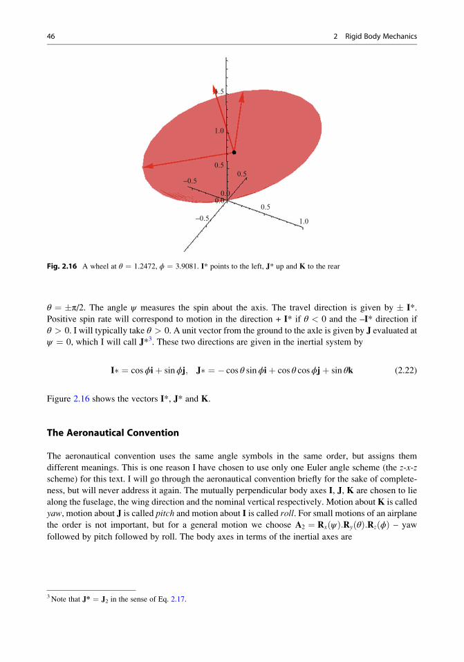
θ ¼ �π/2. The angle ψ measures the spin about the axis. The travel direction is given by � I*.

Positive spin rate will correspond to motion in the direction + I* if θ < 0 and the –I* direction if

θ > 0. I will typically take θ > 0. A unit vector from the ground to the axle is given by J evaluated atψ ¼ 0, which I will call J*3. These two directions are given in the inertial system by

I� ¼ cosϕiþ sinϕj; J� ¼ � cos θ sinϕiþ cos θ cosϕjþ sin θk (2.22)

Figure 2.16 shows the vectors I*, J* and K.

The Aeronautical Convention

The aeronautical convention uses the same angle symbols in the same order, but assigns them

different meanings. This is one reason I have chosen to use only one Euler angle scheme (the z-x-zscheme) for this text. I will go through the aeronautical convention briefly for the sake of complete-

ness, but will never address it again. The mutually perpendicular body axes I, J, K are chosen to lie

along the fuselage, the wing direction and the nominal vertical respectively. Motion aboutK is called

yaw, motion about J is called pitch and motion about I is called roll. For small motions of an airplane

the order is not important, but for a general motion we choose A2 ¼ Rx ψð Þ:Ry θð Þ:Rz ϕð Þ – yaw

followed by pitch followed by roll. The body axes in terms of the inertial axes are

0.00.0

0.5

0.50.5

1.0

1.0

1.5

−0.5

−0.5

Fig. 2.16 A wheel at θ ¼ 1.2472, ϕ ¼ 3.9081. I* points to the left, J* up and K to the rear

3 Note that J* ¼ J2 in the sense of Eq. 2.17.


I ¼cos θ cosϕ

cos θ sinϕ

sin θ

8><>:

9>=>;

J ¼� sinϕ cosψ � cosϕ sin θ sinψ

cosϕ cosψ � sinϕ sin θ sinψ

cos θ sinψ

8><>:

9>=>;

K ¼sinϕ sinψ � cosϕ sin θ cosψ

� cosϕ sinψ � sinϕ sin θ cosψ

cos θ cosψ

8><>:

9>=>;

ð2:110Þ

and the rotation rate in inertial coordinates is

ω ¼� _θ sinϕþ _ψ cosϕ cos θ_θ cosϕþ _ψ sinϕ cos θ

_ϕ� _ψ sin θ

8<:

9=; ð2:12b0Þ

The Combined Rotations as a Single Rotation

Applying the Euler rotations (in the z-x-z convention) leads to a combined rotation matrix: R ¼Rz(ψ).Rx(θ).Rz(ϕ). This rotation can be written as a single rotation through an angle Ω about a single

axis. This is not part of the mainstream of this text, but it is an interesting fact worth exploring for

completeness. Denote the single rotation axis by a. Rotation about a does not rotate the axis itself, so

we have the equation

R:a ¼ a (2.23)

which states that R has an eigenvalue +1 and an eigenvector a. The rotation axis is then proportional

to the eigenvector of R for which +1 is the eigenvalue. The unnormalized eigenvector is

a ¼cos

ϕ� ψ

2

� �csc

ϕþ ψ

2

� �tan

θ

2

sin ϕ� ψð Þ tan θ2

sinϕþ sinψ1

8>>>><>>>>:

9>>>>=>>>>;

(2.24)

It is possible by a proper rotation to transform R to a simple rotation about a. Suppose the new

coordinate system to be such that a ¼ k. Then the rotation can be written in that coordinate system as

R0 Ωð Þ ¼cosΩ � sinΩ 0

sinΩ cosΩ 0

0 0 1

8<:

9=; (2.25)

Kinematics 47

The trace of this rotation matrix can be used to find Ω, but the trace of a matrix is invariant under

proper rotations, so the trace of R0 is equal to the trace of R, and we have an equation for the single

rotation angle corresponding to the three Euler angles:

Ω ¼ cos�1 Tr Rð Þ � 1

2

� �(2.26)

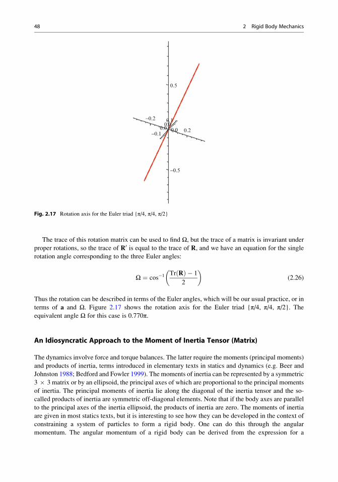
Thus the rotation can be described in terms of the Euler angles, which will be our usual practice, or in

terms of a and Ω. Figure 2.17 shows the rotation axis for the Euler triad {π/4, π/4, π/2}. Theequivalent angle Ω for this case is 0.770π.

An Idiosyncratic Approach to the Moment of Inertia Tensor (Matrix)

The dynamics involve force and torque balances. The latter require the moments (principal moments)

and products of inertia, terms introduced in elementary texts in statics and dynamics (e.g. Beer andJohnston 1988; Bedford and Fowler 1999). The moments of inertia can be represented by a symmetric

3 � 3 matrix or by an ellipsoid, the principal axes of which are proportional to the principal moments

of inertia. The principal moments of inertia lie along the diagonal of the inertia tensor and the so-

called products of inertia are symmetric off-diagonal elements. Note that if the body axes are parallel

to the principal axes of the inertia ellipsoid, the products of inertia are zero. The moments of inertia

are given in most statics texts, but it is interesting to see how they can be developed in the context of

constraining a system of particles to form a rigid body. One can do this through the angular

momentum. The angular momentum of a rigid body can be derived from the expression for a

0.00.00.00.1

0.5

0.2

−0.5

−0.1

−0.2

Fig. 2.17 Rotation axis for the Euler triad {π/4, π/4, π/2}


collection of particles. Doing this will also give us the moments and products of inertia in the form of

an inertia tensor. This is a generalization of the exposition given in elementary statics texts.

The angular momentum for a collection of particles is given by Eq. 1.23, reproduced here for

convenience

l ¼ R� r0ð Þ � mVþXNi¼1

mir0i � v0i (1.23)

I care about the second term, which is the angular momentum of the rigid body with respect to its

center of mass. If R ¼ r0 (r0 is at the center of mass), it is the total angular momentum. The only

relative motion possible for particles in a rigid body is rotation, here rotation about the center of mass.

The rotation vector is the same everywhere in the rigid body, and we can write

XNi¼1

mir0i � v0i ¼

XNi¼1

mir0i � Ω� r0ið Þ )

ðvolume

ρr0 � Ω� r0ð ÞdV (2.27)

where Ω denotes the (instantaneously fixed) rotation vector. The double cross product can be

rewritten using a common vector identity (see, e.g., Stratton 1941) to give

ðvolume

ρr0 � ðΩ� r0ÞdV ¼ Ωðvolume

ρr0 � r0dV �ðvolume

ρðΩ � r0ÞrdV (2.28)

This is a vector, and it is equal to the inertia tensor times the rotation vector, although that is not

immediately obvious. Indicial notation (see Appendix A) can make this much clearer. The following

is not the only route through, but it works very nicely. Rewrite the angular momentum in indicial

notation, dropping the prime on the r as unnecessary as long as we remember what we are doing (that

is, that r represents the radius vector with respect to the center of mass). Then

li ¼ Ωj

ðvolume

ρδjirkrkdV � Ωj

ðvolume

ρrirjdV ¼

ðvolume

ρ δjirkrk � rir

j� �

dV

Ωj ¼ IjiΩj (2.29)

where δji denotes the Kronecker delta, equal to zero when i and j are not equal and unity when they

are. I leave it to the reader to show that the inertia tensor contains the moments of inertia when i ¼ j

and the products of inertia otherwise. The inertia tensor is symmetric, and so there exists an

orientation for which it is purely diagonal. Body axes oriented in this position are called principal

axes, and one tries to choose principal axes for analysis.

We can do the same sort of analysis for kinetic energy. We’ve shown that the kinetic energy for a

collection of particles is

T ¼ 1

2mV � Vþ

XNi¼1

1

2miv

0i � v0i (1.27)

As before, the only motion possible in a rigid body is rotation. Choose the center of mass to be the

reference point and write

T ¼ 1

2mV � Vþ 1

2

XNi¼1

mivi � vi ) 1

2mV � Vþ 1

2

ðvolume

ρ Ω� rð Þ � Ω� rð ÞdV (2.30)

Kinematics 49

http://dx.doi.org/10.1007/978-1-4614-3930-1_9

We can rewrite the latter integral using the relevant vector identity, and then introduce indicial

notation to obtain

ðvolume

1

2ρ Ω� rð Þ � Ω� rð ÞdV ¼ 1

2

ðvolume

ρ Ω � Ωð Þ r � rð Þ � Ω � rð Þ2� �

dV

¼ 1

2Ωi

ðvolume

ρ δijrkrk � rirj

� �dVΩj ¼ 1

2ΩiI

ijΩ

j

(2.31)

showing that the kinetic energy of rotation can be expressed in terms of the rotation and the inertia

tensor. These expressions are simpler in principal axes, for which there are no products of inertia (off-

diagonal terms in the inertia matrix), and we will generally work in principal (body) coordinates.

Denote the principal moments of inertia by A, B and C. The angular momentum is given in body

coordinates4 by

l ¼ A _ϕ sin θ sinψ þ _θ cosψ� �

Iþ B _ϕ sin θ cosψ � _θ sinψ� �

Jþ C _ϕ cos θ þ _ψ� �

K (2.32)

and the (rotational) kinetic energy by

Trot ¼ 1

2A _ϕ sin θ sinψ þ _θ cosψ� �2 þ 1

2B _ϕ sin θ cosψ � _θ sinψ� �2 þ 1

2C _ϕ cos θ þ _ψ� �2

(2.33)

The total kinetic energy is this plus the translational kinetic energy associated with the motion of the

center of mass, which we can write as

Ttrans ¼ 1

2m _x2 þ _y2 þ _z2� �

(2.34)

Note that both the translational and rotational kinetic energies are quadratic forms in the

derivatives of the coordinates. We can combine the two into a single quadratic form involving all

six coordinates. We can combine the coordinates by defining generalized coordinates q

qi ¼ x y z θ ϕ ψf g , qi ¼ x y z θ ϕ ψf gT (2.35a)

Equivalently

q1 ¼ x ¼ q1; q2 ¼ y ¼ q2; q3 ¼ z ¼ q3; q4 ¼ ϕ ¼ q4; q5 ¼ θ ¼ q5; q6 ¼ ψ ¼ q6 (2.35b)

(This is not a unique choice, but it is a common one.) Because the kinetic energy is a quadratic form it

can be written as

T ¼ 1

2_qiMij _q

j (2.36)

4 The full expression in inertial coordinates is much too unwieldy for display.


The matrix Mij is a 6 � 6 invertible symmetric matrix, and it represents the inertia of the system.

In general it depends on the coordinates, but not their derivatives. It is not the same as the inertia

matrix of a single rigid body. It can be called the inertia matrix for the system. I will generally refer toit as the inertia for short. It is a 6 � 6 matrix for the single unconstrained rigid body. It can be larger

or smaller for real systems, as we will see going forward. The system inertia matrix for a single rigid

body may be written in terms of qi

m 0 0 0 0 0

0 m 0 0 0 0

0 0 m 0 0 0

0 0 0 A cos2 q6 þ Bsin2q6 A� Bð Þ sin q4 sin q6 cos q6 0

0 0 0 A� Bð Þ sin q4 sin q6 cos q6 C cos2 q4 þ A sin2 q6 þ Bcos2q6� �

sin2q4 C cos q4

0 0 0 0 C cos q4 C

8>>>>>>>>>><>>>>>>>>>>:

9>>>>>>>>>>=>>>>>>>>>>;

(2.37)

There is obviously significant simplification if the body is axisymmetric so that A ¼ B.

The location of a point in a rigid body with respect to the center of mass can be written

R ¼ XIþ YJþ ZK (2.38)

The motion of the point with respect to the center of mass, which defines the angular velocity of the

body, is the rate of change of R and this can be written in two ways:

Vrot ¼ Ω� R ¼ _R (2.39)

Expanding these two expressions leads to

ΩYZ�ΩZY¼ YI � _JþZI � _K; ΩZX�ΩXZ¼XJ � _IþZJ � _K; ΩXY�ΩYX¼XK � _IþYK � _J (2.40)

from which we can find the components of the angular velocity in the body frame:

ΩX ¼ d

dYK � _R� �

; ΩY ¼ d

dZI � _R� �

; ΩZ ¼ d

dXJ � _R� �

(2.41)

Thus if we know the body axes in terms of any set of coordinates, we can find the angular velocity,

momentum and kinetic energy in terms of those coordinates. The reader might find it informative to

verify Eq. 2.41 for the case for which the coordinates are the Euler angles. You should be able to

reproduce Eq. 2.21a.

Dynamics

We now have everything we need to know to write the equations of motion for an unconstrained rigid

body. We will use the simple rigid body as a building block as we move forward. Do not be

Dynamics 51

intimidated by the apparent complexity in the Euler-Lagrange formulation. We will find simpler

equivalent formulations later.

The potential is a function only of the coordinates, not their derivatives, so the Lagrangian can be

written compactly as

L ¼ 1

2_qiMij q

k� �

_qj � V qk� �

(2.42)

The nondissipative Euler-Lagrange equations from Chap. 1 are

d

dt

@L

@ _qk

� �� @L

@qk¼ QNPk (1.44)

This suggests a convenient bit of notation

pk ¼ @L

@ _qk¼ Mkj _q

j (2.43)

This is called the conjugate momentum. Note that the free index is a subscript so that this is a row

vector. For now it is just a convenient bit of shorthand, but it will come into its own in Chap. 4.

The Euler-Lagrange equations can be written

_pk �@L

@qk¼ Mkj€q

j þ @Mkj

@qm_qm _qj ¼ Qk (2.44)

(Remember that at this point pk is just convenient shorthand as defined in Eq. 2.43.) There will be sixEuler-Lagrange equations for an unconstrained rigid body. The first three are simple; the second three

are coupled. I write them in terms of q and its first two derivatives. The first three are simply

m€qi þ@V

@qi¼ Qi; i ¼ 1; 2; 3 (2.45a,b,c)

The angular equations are fairly complicated. We’ll find easier ways to deal with them eventually,

but for now, let’s simply write them out one at a time

d

dtA cos2 q6 þ Bsin2q6� �

_q4 þ A� Bð Þ sin q4 sin q6 cos q6 _q5� �þ cos q4 sin q4 C� Bcos2q6 � Asin2q6

� �_q5

2 þ C sin q4 _q5 _q6 � A� Bð Þ cos q4 sin q6 cos q6 _q4 _q5 ¼ Q4

(2.45d)

d

dtA� Bð Þ sin q4 sin q6 cos q6 _q4 þ sin2 q4 A sin2 q6 þ Bcos2q6

� �þ Ccos2q4� �

_q5 þ C cos q4 _q6� � ¼ Q5

(2.45e)

Cd

dtcos q4 _q5 þ _q6� �þ A� Bð Þ cos q6 sin q6 _q4

2 � sin2q4 _q52

� �� cos2 q6 � sin2q6� �

sin q4 _q4 _q5� �

¼ Q6

(2.45f)


http://dx.doi.org/10.1007/978-1-4614-3930-1_1

http://dx.doi.org/10.1007/978-1-4614-3930-1_4

Chapter 1 introduced the generalized forces. One way to find them is by using a virtual displacement

procedure. Imagine each component of q to be given a small virtual displacement without the other

components changing. The force or torque that does virtual work during this virtual displacement is the

generalized force that goes with that component of q, and appears in the corresponding dynamical

equation. This needs to be modified a bit when we get to constrained motion in Chap. 3, but it is worth

noting here to give us a head start.

Similar equations (in terms of torques in the inertial system rather than generalized forces) are

often given in elementary dynamics books (e.g. Bedford and Fowler 1999, Eq. 9.48). There is

significant simplification for axisymmetric bodies for which A and B are equal, and some additional

simplification for spherically symmetric bodies (not necessarily spheres – the inertia ellipsoid of a

cube is a sphere). The general problem is ghastly. I will address it in a different setting later. It can be

dealt with numerically as posed. One would have to solve for the second derivatives in Eq. 2.45 d–f,

give the first derivatives names and proceed to a 12 dimensional state space. There are several better

ways to address this particular problem, and we will examine several of these in Chap. 4. We can find

some interesting things by looking at some examples using Eq. 2.45 a–f.

Applications/Examples

Example 2.1 A Falling Brick. Consider a rectangular brick, semiaxes a, b and c, massM and principal

moments of inertia A, B and C falling under gravity. Let z be positive up, so that the potential energy is

Mgz, where g denotes the acceleration of gravity. The kinetic energy is the sum of the energies given

by Eqs. 2.26 and 2.27. I will assign the generalized coordinates according to Eq. 2.28. There are no

generalized forces, and we can write the six Euler-Lagrange equations from Eq. 2.34. The transla-

tional ones are simple and not coupled to the rotational equations:

M€q1 ¼ 0 ¼ M€q2; M€q3 þMg ¼ 0

These tell us that the brick falls down under gravity, and translates sideways at a uniform speed. (This

is the same behavior as the projectile of Example 1.2; rotation does not affect this behavior, although

it may well affect the stability of the motion.) The others are homogeneous, Eq. 2.45 d–f with no

generalized forces and no explicit appearance of q5. These equations are still complicated coupled

nonlinear ordinary differential equations. There are no general analytic solutions, and numerical

solution is complicated. The Euler-Lagrange equations as stated are not the best way to address this

problem, but one can say a few things from this formulation.

Any set of constant angles satisfies these equations. Spin about the K axis is easily represented by

the rate of change of ψ , and such a spin also satisfies the equations. It is apparently well-known

(Goldstein (1980, pp. 209–10) touches on this) that such a spin will be stable if theK direction has the

largest or smallest principal moment of inertia, but unstable if the axis is an intermediate axis, that is,

C must be less than A and B or greater than A and B for this spin to be stable. ([C < (A&B)] OR

[C > (A&B)] implies stability.) This can be demonstrated numerically using the equations of motion,

which I will do here, and it is possible to set up a linearized system of equations to prove infinitesimal

stability/instability, but that is very intricate. The proof is simple using the method of

quasicoordinates, and I will defer the proof until we have explored that in Chap. 4.

Numerical solution of these problems is usually effected by writing the governing equations as a

set of first order ordinary differential equations and using an appropriate numerical scheme (usually

one of the variants of the Runge–Kutta method, see Press et al. 1992) to integrate them. To solve this

Applications/Examples 53

http://dx.doi.org/10.1007/978-1-4614-3930-1_1

http://dx.doi.org/10.1007/978-1-4614-3930-1_3

http://dx.doi.org/10.1007/978-1-4614-3930-1_4

http://dx.doi.org/10.1007/978-1-4614-3930-1_4

problem numerically using what we know so far, we solve the six Euler-Lagrange equations for €q, let_q ¼ u and then we will have six equations for _q in terms of q and u and another six equations for _u.

These form a twelfth order system that can be integrated numerically5. The u equations are quite

complicated so I will not display them here.

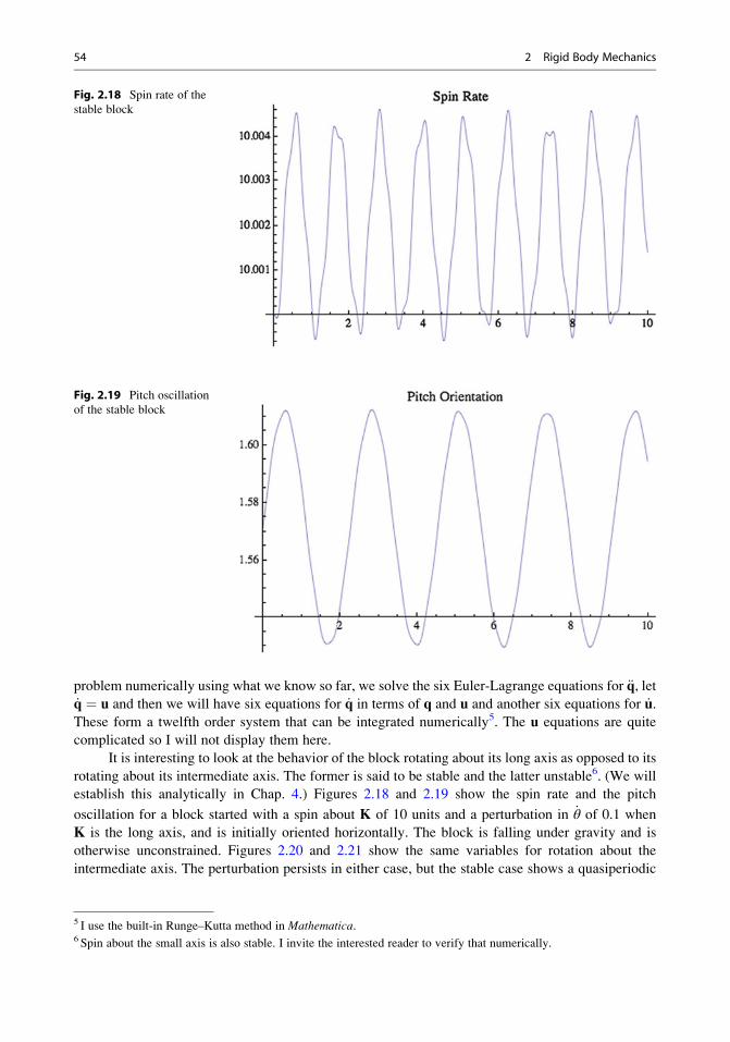
It is interesting to look at the behavior of the block rotating about its long axis as opposed to its

rotating about its intermediate axis. The former is said to be stable and the latter unstable6. (We will

establish this analytically in Chap. 4.) Figures 2.18 and 2.19 show the spin rate and the pitch

oscillation for a block started with a spin about K of 10 units and a perturbation in _θ of 0.1 when

K is the long axis, and is initially oriented horizontally. The block is falling under gravity and is

otherwise unconstrained. Figures 2.20 and 2.21 show the same variables for rotation about the

intermediate axis. The perturbation persists in either case, but the stable case shows a quasiperiodic

Fig. 2.18 Spin rate of the

stable block

Fig. 2.19 Pitch oscillation

of the stable block

5 I use the built-in Runge–Kutta method in Mathematica.6 Spin about the small axis is also stable. I invite the interested reader to verify that numerically.


http://dx.doi.org/10.1007/978-1-4614-3930-1_4

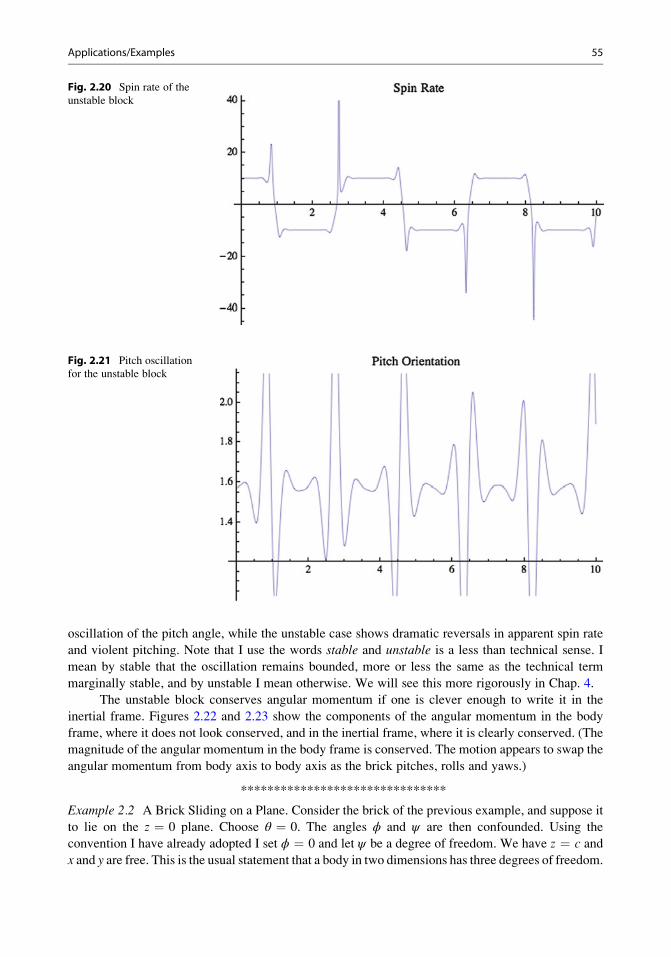
oscillation of the pitch angle, while the unstable case shows dramatic reversals in apparent spin rate

and violent pitching. Note that I use the words stable and unstable is a less than technical sense. I

mean by stable that the oscillation remains bounded, more or less the same as the technical term

marginally stable, and by unstable I mean otherwise. We will see this more rigorously in Chap. 4.

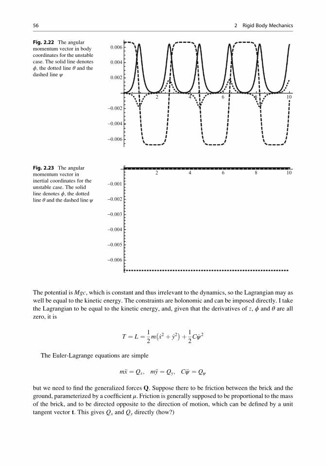
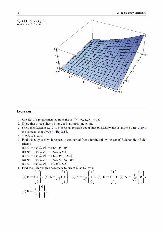
The unstable block conserves angular momentum if one is clever enough to write it in the

inertial frame. Figures 2.22 and 2.23 show the components of the angular momentum in the body

frame, where it does not look conserved, and in the inertial frame, where it is clearly conserved. (The

magnitude of the angular momentum in the body frame is conserved. The motion appears to swap the

angular momentum from body axis to body axis as the brick pitches, rolls and yaws.)

*******************************

Example 2.2 A Brick Sliding on a Plane. Consider the brick of the previous example, and suppose it

to lie on the z ¼ 0 plane. Choose θ ¼ 0. The angles ϕ and ψ are then confounded. Using the

convention I have already adopted I set ϕ ¼ 0 and let ψ be a degree of freedom. We have z ¼ c and

x and y are free. This is the usual statement that a body in two dimensions has three degrees of freedom.

Fig. 2.20 Spin rate of the

unstable block

Fig. 2.21 Pitch oscillation

for the unstable block


http://dx.doi.org/10.1007/978-1-4614-3930-1_4

The potential isMgc, which is constant and thus irrelevant to the dynamics, so the Lagrangian may as

well be equal to the kinetic energy. The constraints are holonomic and can be imposed directly. I take

the Lagrangian to be equal to the kinetic energy, and, given that the derivatives of z, ϕ and θ are all

zero, it is

T ¼ L ¼ 1

2m _x2 þ _y2� �þ 1

2C _ψ2

The Euler-Lagrange equations are simple

m€x ¼ Qx; m€y ¼ Qy; C€ψ ¼ Qψ

but we need to find the generalized forces Q. Suppose there to be friction between the brick and the

ground, parameterized by a coefficient μ. Friction is generally supposed to be proportional to the mass

of the brick, and to be directed opposite to the direction of motion, which can be defined by a unit

tangent vector t. This gives Qx and Qy directly (how?)

−0.006

−0.004

−0.002

0.002

2 4 6 8 10

0.004

0.006Fig. 2.22 The angular

momentum vector in body

coordinates for the unstable

case. The solid line denotes

ϕ, the dotted line θ and the

dashed line ψ

−0.006

−0.005

−0.004

−0.003

−0.002

−0.001

2 4 6 8 10Fig. 2.23 The angular

momentum vector in

inertial coordinates for the

unstable case. The solid

line denotes ϕ, the dottedline θ and the dashed line ψ


Qx ¼ � _xffiffiffiffiffiffiffiffiffiffiffiffiffiffi_x2 þ _y2

p μmg; Qy ¼ � _yffiffiffiffiffiffiffiffiffiffiffiffiffiffi_x2 þ _y2

p μmg

Friction also opposes the rotation, but to find that torque we need to integrate. This is fairly messy.

Before we go to that note that the translational equations decouple from the rotational equation

(as they did in the more general Example 2.1). The translational equations have a closed form solution

over a limited time for an initially translating block. One can substitute the generalized forces into the

Euler-Lagrange equations to form a single equation for the speed of the block

m _x€xþ m _y€y ¼ � _x2ffiffiffiffiffiffiffiffiffiffiffiffiffiffi_x2 þ _y2

p μmg� _y2ffiffiffiffiffiffiffiffiffiffiffiffiffiffi_x2 þ _y2

p μmg

+1

2

d

dt_x2 þ _y2

� � ¼ �μgffiffiffiffiffiffiffiffiffiffiffiffiffiffi_x2 þ _y2

q

This can be integrated by separation of variables and the result is

ffiffiffiffiffiffiffiffiffiffiffiffiffiffi_x2 þ _y2

q¼ v ¼ v0 � 4μgt

which tells us that a sliding block will stop sliding when t ¼ v0/4 μg. Here v0 denotes the initial

velocity. The solution is meaningless for larger times.

The rotational frictional torque Qψ is given by

τk ¼ðð�area

r� ð�tμdmÞ ¼ðð�area

r� ð�tμÞρ2cdA

where ρ denotes the density of the brick, r a vector from the center of mass to a point on the surface

and t the unit tangent vector to the motion. The tangent vector is given by t ¼ (k� r)/r, where r is themagnitude of r. This can be converted using the usual vector identities (e.g. Stratton 1941), giving

τ ¼ �8μρgc

ðb0

ða0

ffiffiffiffiffiffiffiffiffiffiffiffiffiffiffiffiX2 þ Y2

pdXdY

I have written the integral in body coordinates for convenience and made use of symmetry to write

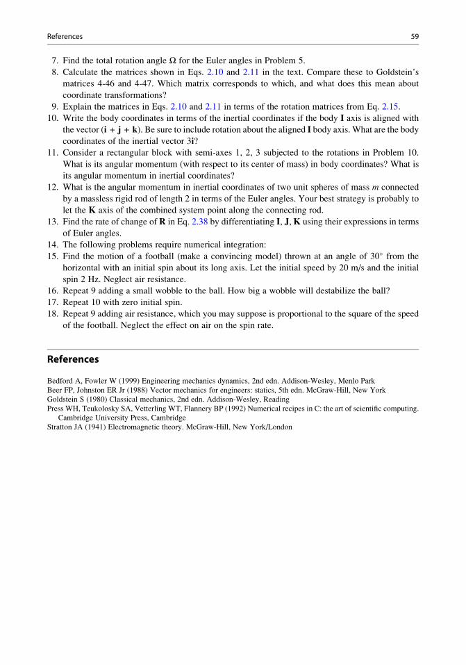
it as four times the integral over one quadrant. This is a nontrivial integral, but Mathematica knows it.

I won’t write the result, but Fig. 2.24 shows its value as a function of a and b. It is, in any case,

constant, and the rotation equation is simple and the result is

ψ ¼ ψ0 þ _ψ0t�1

2τt2

valid until _ψ first becomes zero, at which point the spin stops. Both translational and rotational sliding

stop in finite time.

Note that this friction force is nonlinear and cannot be incorporated in a Rayleigh dissipation

function. Only the so-called viscous friction, f ¼ �kv, can be modeled using a Rayleigh dissipation

function.


Exercises

1. Use Eq. 2.1 to eliminate z2 from the set {x1, y1, z1, x2, y2, z2}.

2. Show that three spheres intersect in at most one point.

3. Show that Rx(α) in Eq. 2.11 represents rotation about an x axis. Show that A1 given by Eq. 2.20 is

the same as that given by Eq. 2.14.

4. Verify Eq. 2.19.

5. Find the body axes with respect to the inertial frame for the following sets of Euler angles (Euler

triads):

(a) Φ ¼ {ϕ, θ, ψ} ¼ {π/4, π/4, π/4}(b) Φ ¼ {ϕ, θ, ψ} ¼ {π/3, 0, π/3}(c) Φ ¼ {ϕ, θ, ψ} ¼ {π/3, π/4, �π/3}(d) Φ ¼ {ϕ, θ, ψ} ¼ {π/3, π/100, �π/3}(e) Φ ¼ {ϕ, θ, ψ} ¼ {0, π/2, π/2}

6. Find the Euler angles necessary to orient K as follows:

ðaÞ K ¼0

1

0

8><>:

9>=>;; ðbÞ K¼ 1ffiffiffi

3p

1

1

1

8><>:

9>=>;; ðcÞ K¼ 1ffiffiffi

2p

1

1

0

8><>:

9>=>;; ðdÞ K¼

1

0

0

8><>:

9>=>;; ðeÞ K ¼ 1ffiffiffi

2p

1

0

1

8><>:

9>=>;;

ðfÞ K¼ 1ffiffiffi2

p0

1

1

8><>:

9>=>;;

0.0

0.00

2

4

6

0.5

0.5

1.0

1.0

1.5

1.5

2.0

2.0

Fig. 2.24 The τ integralfor 0 < a < 2, 0 < b < 2


7. Find the total rotation angle Ω for the Euler angles in Problem 5.

8. Calculate the matrices shown in Eqs. 2.10 and 2.11 in the text. Compare these to Goldstein’s

matrices 4-46 and 4-47. Which matrix corresponds to which, and what does this mean about

coordinate transformations?

9. Explain the matrices in Eqs. 2.10 and 2.11 in terms of the rotation matrices from Eq. 2.15.

10. Write the body coordinates in terms of the inertial coordinates if the body I axis is aligned with

the vector (i + j + k). Be sure to include rotation about the aligned I body axis. What are the body

coordinates of the inertial vector 3i?

11. Consider a rectangular block with semi-axes 1, 2, 3 subjected to the rotations in Problem 10.

What is its angular momentum (with respect to its center of mass) in body coordinates? What is

its angular momentum in inertial coordinates?

12. What is the angular momentum in inertial coordinates of two unit spheres of mass m connected

by a massless rigid rod of length 2 in terms of the Euler angles. Your best strategy is probably to

let the K axis of the combined system point along the connecting rod.

13. Find the rate of change of R in Eq. 2.38 by differentiating I, J,K using their expressions in terms

of Euler angles.

14. The following problems require numerical integration:

15. Find the motion of a football (make a convincing model) thrown at an angle of 30� from the

horizontal with an initial spin about its long axis. Let the initial speed by 20 m/s and the initial

spin 2 Hz. Neglect air resistance.

16. Repeat 9 adding a small wobble to the ball. How big a wobble will destabilize the ball?

17. Repeat 10 with zero initial spin.

18. Repeat 9 adding air resistance, which you may suppose is proportional to the square of the speed

of the football. Neglect the effect on air on the spin rate.

References

Bedford A, Fowler W (1999) Engineering mechanics dynamics, 2nd edn. Addison-Wesley, Menlo Park

Beer FP, Johnston ER Jr (1988) Vector mechanics for engineers: statics, 5th edn. McGraw-Hill, New York

Goldstein S (1980) Classical mechanics, 2nd edn. Addison-Wesley, Reading

Press WH, Teukolosky SA, Vetterling WT, Flannery BP (1992) Numerical recipes in C: the art of scientific computing.

Cambridge University Press, Cambridge

Stratton JA (1941) Electromagnetic theory. McGraw-Hill, New York/London

References 59

http://www.springer.com/978-1-4614-3929-5