- 1 -

Real Estate Risk:A Forward Looking Approach

By

William C. Wheaton, Ph.D.Raymond G. Torto, Ph.D., CRE

Petros S. Sivitanides, Ph.D.Jon A. Southard

Robert E. HopkinsJames M. Costello

Torto Wheaton Research200 High Street

Boston, MA 02110-3036www.tortowheatonresearch.com

617-912-5200

May15, 2001

� Torto Wheaton Research, 2001

- 2 -

Real Estate Risk:A Forward Looking Approach

Executive Summary: In this paper we argue forcefully that real estate is a predictable

asset class (unlike stocks and bonds} and propose a forward-looking methodology for

evaluating real estate market risk. Using a modern time-series modeling approach, VAR, we

argue that it is possible to quantify such risk, as the standard error of the forecast for each

variable in a real estate model. Subsequently, we outline an approach for assessing income

and value risk in commercial real estate, based on the premise that the most important source

of such risk is the market’s fundamentals. Finally we demonstrate the application of this

approach in generating confidence bands for NOI and property values for specific markets.

1. Introduction

Investors in real estate, public or private, equity or debt, evaluate risk adjusted returns

in the pursuit of their goals. Or, at least, that is what they profess! More often the real estate

practice is to evaluate investment returns, not risk adjusted investment returns.

Practice focuses on returns, not risk adjusted returns, not because the real estate

investor hasn’t read his/her finance books, but because of the lack of appropriate risk

measures that can be usefully applied to real estate.

This paper is one of three that we have prepared to address this problem. We develop

a forward looking methodology to define and measure risk in real estate and to apply it to

- 3 -

equity (private or public) and debt (private or public). This paper, the first in the trilogy,

introduces our thinking on how to define and generate risk measures for real estate that can be

used for fundamental analysis (as it relates to leasing markets) and investment analysis (asset

related).1

This paper is a further evolution of our thinking found in (Wheaton et al., 1999) and

has benefited immeasurably from discussions with fellow academics, researchers, and many

clients of Torto Wheaton Research.2 Readers familiar with our previous writings on this

subject will find parts of this earlier discussion interspersed herein. We felt it was important

to present our full, complete and significantly revised methodology in one paper.

This paper first reviews some traditional definitions and measures of real estate

investment risk, and then proposes a forward-looking and useful methodology for forecasting

and evaluating real estate market risk. Our primary contribution is to argue that for real estate

markets, which have some significant degree of statistical predictability, the uncertainty

associated with forecasting of market outcomes, and not the inherent, historical variability of

the market itself, is the key measure of risk. As we will demonstrate this forecast uncertainty

comes from a number of sources-- the local or national economy, net absorption, new

construction, rents, vacancy-- each of which contribute to generating uncertainty about future

market outcomes-- the true definition of risk. But we will also argue that the most important

distinction to make for real estate is to separate the predictable versus unpredictable

components in forecasting real estate markets.

2. Future Market Uncertainty is Risk

- 4 -

Most economists agree that risk is best conceptualized as uncertainty over likely future

outcomes (Bodie, Kane and Markus, 1993). The future outcome could be thought of as

returns over five years and the uncertainty can be thought of as a “deviation” from an

expected, or likely outcome. Over the past forty years the exploration of risk has been one of

the dominant themes of financial economics and the success of this line of inquiry is evident

in that the technical advances in financial economics have been applied to nearly all other

branches of the discipline.

A detailed review of this literature is beyond the scope of this paper. Instead, it is

sufficient to note that risk is generally modeled as some function of the “spread” of the

probability distribution of future outcomes (Sharpe, 1985).3 Economists or finance theorists

do not debate the definition of risk, but rather the challenges surrounding its measurement and

its application. On this theme, the next section introduces our perspective on measuring real

estate risk.

3. Measuring Real Estate Risk: Market Variability vs. Future Uncertainty

If there is so much agreement that risk is the uncertainty of future outcomes, why,

then, is historical variability the most often used measure of investment risk? For instance, in

publicly traded securities markets, analysts frequently look at the historical variability of

investment returns as one principal measure of risk. This is usually measured by the standard

deviation of historical returns.

The answer lies in the pricing nature of publicly traded securities. These markets are

widely held to be efficient. That is, the current price reflects all information available and, as

such, public market returns are largely a random walk (Fama, 1965).

- 5 -

Think of it this way. Historical variability can be decomposed into two components: a

predictable part and a non-predictable or “intrinsic” variability. The predictable component is

displayed in the historical return series when there are autoregressive or other distinct

statistical patterns. The unpredictable component is evidenced in time series that have more

of a random walk. Publicly traded securities markets are widely held to be efficient and, as

such, it is believed that they have little predictable component. Hence, if returns are largely a

random walk, then future returns cannot be reliably predicted and using historical data to

estimate variability is acceptable.4

The key question is whether real estate risk should be defined, measured and

estimated as it has been done in the public securities markets? The problem with extending

Wall Street methods to real estate is that this asset class exhibits predictable auto-correlation

over time. For instance, property income is highly auto-correlated due to long term leasing

contracts. Furthermore, with development lags, even positive random market shocks always

set off a predictable rise and then eventually a fall in asset prices. Numerous researchers have

documented the unusually strong predictable component in real estate markets (e.g., Shiller

and Case, 1989).

Our argument is that since there are predicable components to real estate returns,

these returns and the risks can and should be forecast forward, rather than simply

developing a measure reflecting their historical variability.5

4. The Uncertainty of Real Estate Forecasts

A forecast of future real estate investment returns has two components: the variability

of the forecast return and the uncertainty surrounding that forecast. The variability of the

- 6 -

future forecast by definition is based only on the predictable component i.e., the forecast

model. The uncertainty of the forecast incorporates all of the random factors (outside of the

model) that generated much of the (unpredictable) historical variability. Lest there be any

doubt about this, look at an econometric forecast for any variable, it is always smoother than

the historical data series being forecasted6.

If the forces influencing the historical movements of an investment are well

understood, then forecast models fit well and the predictable real estate component is large

relative to what is unknown – the unpredictable component . In this case, there is confidence

in the forecast, the confidence interval is tight and there is lower risk (uncertainty).

When the forces underlying a forecasted variable are largely random or unpredictable,

the forecast model has a poor fit, the confidence interval is large and there is considerably

more uncertainty about the true likely outcome. In these cases, it is the uncertainty of the

forecast that generates most of the true future risk, rather than whether the base forecast has

a smooth or varying pattern of returns (Makridakis, Wheelwright and McGee, 1983).

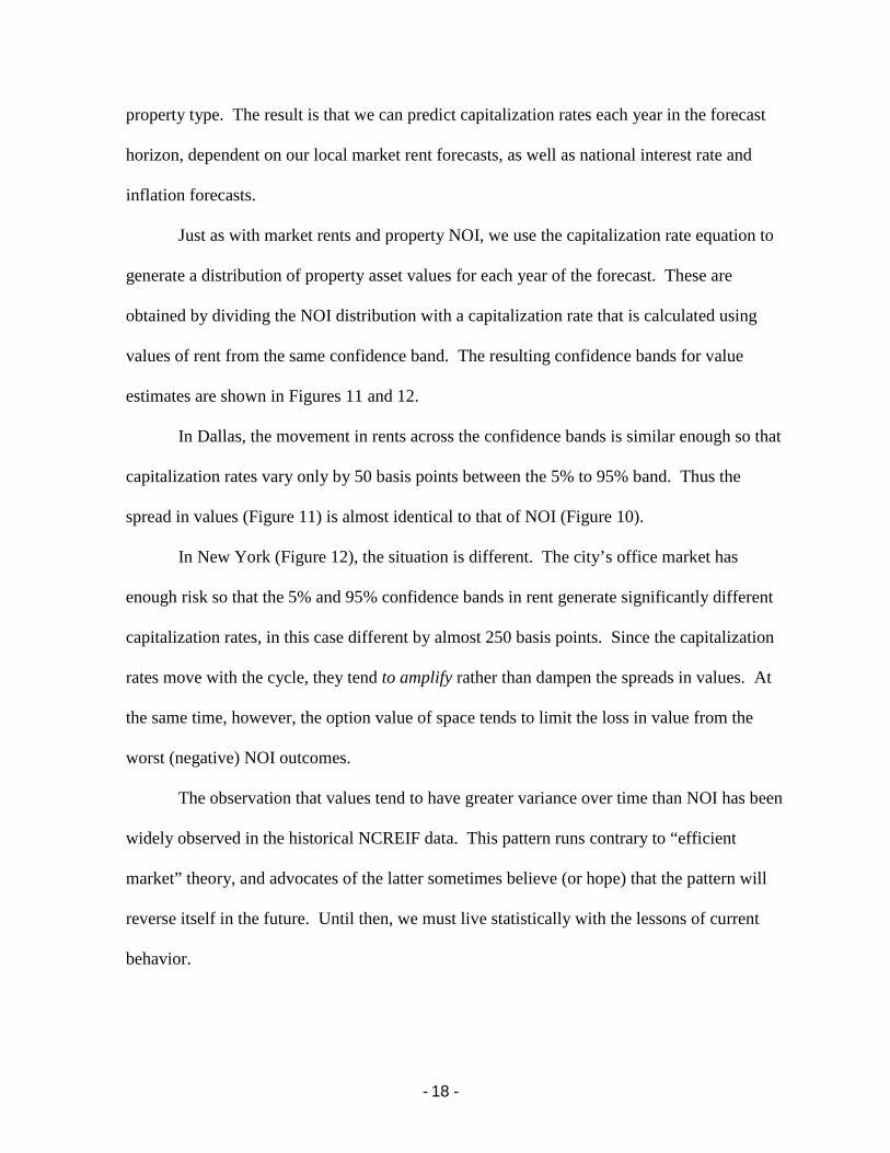
Figure 1 gives an historical and forecasted time series for NOI. This figure illustrates

several points. First, the traditional approach is to take the standard deviation of the historical

variability as a measure of risk. We are arguing that the historical measure will overstate the

future uncertainty because it sums both the predictable and unpredictable components that

generated the historical NOI series. Second, we are arguing that given the current position of

the market or NOI stream, the workings of the real estate market makes real estate more

predictable than the other asset classes.

- 7 -

5. How to Model Real Estate Markets

When investment returns are largely random, as in the traded-security markets, the

“model” which best fits the series is often some (complete or partial) form of Brownian

motion, in which the movement in returns today is independent of previous returns and

largely a function of random error, possibly with a trend.7 The way that such “intrinsic”

variability is forecast, is to simulate the random movements with Monte Carlo methods. After

thousands of trials, one can obtain the frequency distribution of returns for each period

forward in the simulation. If the model is true Brownian motion, the frequency distribution of

returns has increasing spread or variance with time. Since the period to period changes are

random, the simulated movement between year t and t+1 does not depend on the history of

the series through year t. Most economic variables, however, seem to be “bounded,” and so

statisticians use “retaining barriers” and other “mean reverting” techniques to keep the

simulated distribution of outcomes from expanding indefinitely.

It is important to note that in an approach using a Monte Carlo process, the period to

period outcomes are random. That means that if in period six, you forecast NOI to be 100,

then in period seven NOI could be any value—zero, 105 or 1000! We think that for real

estate there is a high correlation over time for NOI or any market variable and, therefore, the

Monte Carlo process is not correct for assessing future uncertainty.

Our view is that real estate markets are not random in their movements. Furthermore,

they have very distinct bounds. For instance, in reaction to positive shocks, new supply

eventually limits the upside for both property income and return. Likewise, with negative

shocks, operating costs and the sunk cost of capital set a floor on returns.

- 8 -

Basically, “mean reversion” is an intrinsic part of the operation of real estate markets.

In reaction to positive shocks, returns initially increase, but eventually diminish with the

arrival of new supply. Similarly, negative shocks lead to building conversions, loss of stock

and an eventual recovery of returns. All of this creates considerable predictability in both

market fundamentals and capital market returns. We believe that good econometric

modeling can capture much of this predictability and that econometric analysis can add

considerably to the analysis of returns and risk in real estate investments in both equity (pubic

and private) and debt (public and private).

5.1. The Torto Wheaton Research (TWR) Approach

This section will introduce our approach on how to measure real estate risk and to

apply it to either collateral specific and/or market prototypical assets in real estate. This

thinking was first introduced in Wheaton, et al. (1999), but has advanced considerably from

that article.

TWR has traditionally modeled the behavior of property markets using a system of

equations that relate local economic drivers to real estate performance measures and to

changes in the asset markets. A simplified sketch of such a system is presented in Figure 2.

Each block in the diagram is an equation and the equations (blocks) interact in terms of

providing explanatory feedback in a recursive manner.

The figure shows the transmission lines from the net absorption model to the rent

model and from the rent model to the construction model. When we estimate these equations

individually, it gives us no ability to determine what percent of the uncertainty surrounding

the construction model is due to unpredictable elements that are feeding through from the

- 9 -

other equations. Such interactions are important if one wants to quantify the predictable vs.

unpredictable portions of an entire system of equations representing a property market and in

turn it’s risk profile.

To capture the interaction between our system of equations, TWR has modeled the

behavior of property markets using Vector Auto Regressive models (VAR). A VAR system

allows one to test the explanatory power of any single variable in a system of equations and

allows us to estimate confidence intervals around the transmission lines. Typically,

forecasters who use VAR systems impose no economic theory on the system of equations that

define their models, and use a VAR system to filter through their data to find variables that

simply work the best (Pindyck and Rubinfeld, 1991).

TWR’s approach, however, has been to use a class of models called “structural”

VARs. Their structure comes from restrictions on the coefficients to conform a priori to

economic theory.8 TWR’s experience in modeling real estate markets gives us the

appropriate structure. Most importantly, for our purposes, linear VAR systems have the

property that confidence intervals of their forecasts can be analytically determined.9 As

opposed to engaging in Monte Carlo random simulations to generate the distribution of

future outcomes (Hamilton, 1996), this approach to determining confidence intervals takes

into account the error structure, or the unpredictable components of each equation in the VAR

system, as well as how these unpredictable components interact through the VAR equations.

Statistically, this means that each variable forecasted in the VAR approach will have a

standard error of the forecast for each period and that each standard error will incorporate

the interrelationships of each equation in the model.

- 10 -

Simply stated, the VAR model estimates a standard error of the forecast, which

incorporates all the components of uncertainty in the estimated model. For instance, the

uncertainty around the rent forecast incorporates the uncertainty of the construction forecast.

Additionally, we can estimate the contributions of each variable to the estimated uncertainty.

The forecasts for each market and the decomposition of the future uncertainty will

depend on a number of considerations and we have a lot of analysis yet to be undertaken. To

date we have found that forecast confidence bandwidths, or standard deviations, depend on

the following market characteristics:

- Markets with long development lags , but with high development elasticity with

respect to rents (that is, markets with a strong supply response in response to rent

changes), tend to exhibit wider confidence intervals since supply responses are

more variable.

- Markets where the underlying determinants of demand and supply are more

idiosyncratic and less explained by rational economic factors, have wider forecast

confidence bands.

- When rent and vacancy forecasts are converted to property net operating income

confidence intervals, the leasing structure and operating parameters of the asset are

extremely important. Shorter leases and greater operating leverage lead to wider

confidence bands for net operating income. This occurs because the property

income becomes more exposed to changes in market conditions.

- 11 -

We will be presenting more analysis of risk across markets and property types in forthcoming

papers.

6. VAR Forecast Confidence Intervals: Some Examples

In order to provide insight to the TWR VAR methodology, we have chosen two

different markets: the New York office market and the Dallas apartment market. These

examples are for illustrative purposes only.

The New York office economy has a large base in the Finance, Insurance, and Real

Estate (FIRE) sector. Since the 1920s, the growth of the securities and banking industries has

seemingly been the “raison d’être” of the city’s economy. Despite this belief, actual FIRE

employment has changed little in the last thirty years. To be sure, it has had its cyclic

movements, but the number of workers in FIRE in 2000 (520,000) is only 8% greater than it

was in 1970. By contrast, employment in the business and professional services category has

increased from 360,000 to more than 660,000 over this same period. This broad category

includes workers employed in sectors ranging from advertising to law to software.

Econometric models of the New York office economy have forecast confidence

intervals that differ greatly by sector. Forecasts of FIRE have very tight confidence bands

around little or no growth. By contrast, forecasts of business and professional services have

much wider confidence bands around a strong upward trend. Thus, much of the future

demand for New York office space rests on the uncertain expansion of the service sector and

not on the growth of its traditional securities and banking industries. Figure 3 shows the VAR

base forecast (the middle line) and confidence bands for business and professional services in

- 12 -

New York. Given the properties of a structural VAR and the application of the Central Limit

Theorem, the sampling distribution of the forecasted variable at any time period is

approximately normally distributed around an expected value for that time period. The

stylized drawing of the normal curve around time period six shows this.

Office construction exhibits far more volatility, some of which is predictable, but

some of which is not. The model suggests that a building boom will occur. Office

development has intrinsically long lags, and so the boom’s magnitude and length are much

harder to predict. In New York, the forecast of 3.5m. square feet of new office space five

years out has a standard deviation of about 1 million square feet, implying that the 95%

confidence band lies between 1.5 and 5.5m. By year ten, the confidence bands are

considerably wider. Figure 4 presents the New York construction forecast and confidence

bands.

The rental forecast for New York, shown in Figure 5, has wide confidence bands, in

part, because the forecasts for two of its major drivers, namely, construction and employment,

also have wide bands. It is pretty clear that the rapid rise in rents will come to an eventual

end, but by the 10th year of the forecast, the 95% confidence bands around the $55 forecast

office rent level range from $75 down to $32. This spread is almost 78% of the forecast

value. Clearly, the New York office market has considerable risk, reflecting its historical

tendency to experience severe cyclical movements.

The Dallas apartment market is different. In Dallas, total employment has risen from

650,000 in 1970 to 1.9 million in 2000. This 200% gain creates a predictable urban growth

trend. As Dallas has gotten bigger, its growth rate has slowed and going forward, most

economists predict that the growth rate in Dallas will slow significantly. By 2009 there will

- 13 -

be 2.35 million workers, only a 25% increase over 2000. Interestingly, the confidence

interval around this forecast is quite tight, at least in comparison to the forecast for New

York’s service sector. The 95% confidence bands for Dallas range from 2.48 to 2.22 million

workers (See Figure 6).

The forecast for apartment construction in Dallas, however, is just as uncertain as the

forecast for office buildings in New York. The recent boom in apartments dropped suddenly

last year, but now exhibits renewed strength. The model forecasts construction to rise

quickly, from 12,000 units to around 18,000 units annually, and then drop back to 10,000

(Figure 7). The confidence bands around this variable, however, are very large, with the 95%

intervals ranging from 24,000 to virtually zero new units. Historically, construction in Dallas

has varied by much more than this range.

What makes Dallas so interesting, however, is that the uncertainty surrounding

apartment construction does not translate into uncertainty in the rent forecast. Rents are

forecast to grow from $620 to about $790 (Figure 8). The 95% confidence band around the

$790 figure for 2009 is from $725 to $825 – only a 16% spread! Some of the tightness in the

rent forecast can be explained by the similar tightness of the economic forecast. However, the

question is: Why is it that uncertainty in supply does not impact the rent confidence bands?

In the apartment market, most of risk historically has originated from unexpected

movements in demand (Wheaton, 1999). Even supply reacts quickly, more quickly than

demand, to changes in the market’s economy. Given the tight forecast bands for Dallas’

economy, rents simply reflect this certainty. When building booms occur, they tend to be

short-lived and coincide with the need for new development. Historically, average apartment

rents in Dallas have not varied by more than 25%, when adjusted for inflation.

- 14 -

By contrast, New York office rents have varied by almost 60% in the last thirty years

(adjusted for inflation). Furthermore, historical office market fluctuations have been closely

linked to long and excessive building booms. In these situations, supply uncertainty creates a

comparable risk or uncertainty for the rent forecast.

7. Translating Market Risk into Property Income Risk

The confidence bands for the New York office and the Dallas apartment market are

interesting, but to be useful for investment decision-making, they must first be translated into

forecast confidence bands corresponding to a specific property’s income stream.

Property income depends on leasing structure. A staggered long-term lease for an

office property can act to smooth the fluctuations the property might otherwise experience due

to changes in market rent. At the same time, the magnitude and growth of operating expenses

creates a leverage effect on gross income, increasing the volatility of net operating income

(NOI) or net cash income.

TWR has developed a discount cash flow model and software program that makes the

conversion from TWR’s market rent and occupancy forecasts to gross income, and then to

NOI, based upon either default or user-supplied, collateral-specific inputs. If the parameters

of a specific property are known, the software will estimate the net income of the specific

asset. If they are not, then prototypical or default parameters are used to develop “generic”

income forecasts for each property type in each market. For this process, we make the

following assumptions:

1). Individual property leases are assumed to rollover at specified periods and the

leases renew at a “market rent” for that building (this can be collateral specific), which moves

- 15 -

with the forecast of market wide rent. The choice of average lease length, or rollover

frequency, varies with the type of property, and is based on the information available in the

TWR leasing database. An allowance is made for lease non-renewals, while the downtime

during re-leasing is based in part on the market wide vacancy rate in that future period. Thus,

each property has its own vacancy rate forecast.

2). Typical operating costs have been obtained from several sources. Additional

allowances are made for tenant improvements after lease non-renewals, as well as for capital

expenses. Using these inputs, building gross income is converted first to NOI, and then after

capital expenses to cash flow. Again, if the user knows the specific operating parameters of a

property, these can be inserted in place of the default values. The software allows for

instantaneous user-defined changes to all variables.

In Figures 9 and 10, this approach is applied to the New York office market and the

Dallas apartment market, discussed in the previous section, using the aforementioned

software. For this example we use a 100,000 square foot office building, and a 200-unit

suburban apartment complex. The results show the NOI forecasts—derived from the “bottom

up”—and depict interesting differences.

The long leases typical of the New York office market mean that changes in property

income lags changes in market rent by several periods (comparing Figure 5 with Figure 10

demonstrates this). While gross property income is considerably smoother than market rents,

office space operating costs represent roughly 40% of current gross income.10 This leverage

tends to render NOI more volatile than gross income. The net effect of these parameters is to

generate NOI confidence bands that are wider than the rent bands. In the 5th year of the

forecast, the 95% NOI confidence intervals have a spread that is 80% of the base forecast. By

- 16 -

the last year of the forecast horizon, the same confidence bands expand to 220% of the base

forecast. These are wider than the 78% spread in market rent.

In the case of Dallas apartments, gross income will almost directly follow market rents

and there is little insulation of income to market rent changes. In addition, the default

operating costs (including capital expenses and arrears) in Dallas that we used average close

to 70% of gross income. The net result of these parameters is that the 95% confidence

intervals exhibit about a 40% spread around the base forecast for most of the forecast time

horizon (Figure 10). In percentage terms, apartment NOI is much more uncertain than market

rent, where the confidence interval spread was only 16% of the base forecast.

8. Translating Income into Value: Forecasting Capitalization Rates

In addition to income risk, another major source of risk in real estate investments is

volatility in asset values. In well-informed liquid asset markets, value (or price) is the present

discounted value of expected future income (or earnings). The ratio of current income to

asset prices, the capitalization rate, varies inversely with expected earnings growth. When

investors can freely trade assets and prices, capitalization rates should vary in equilibrium

only by the degree of income or earnings risk. Specifically, investors cannot diversify that

risk away. Since real estate is not (yet) freely traded, asset prices do not reflect just the asset’s

systematic risk. Numerous authors have shown that real estate asset prices are quite

inefficient, predictable, and do not look forward, but rather backward in forming expectations

about the future (e.g., Hendershott, 2000, Sivitanidou and Sivitanides, 1999, Sivitanides et al.,

2001).

- 17 -

The most widely used data series on asset prices are the NCREIF indices. These

indices report income and appraised values held by some of the nation’s largest institutions.

While appraisal based valuation has been often criticized, actual property transactions are

usually based on some average of the buyer and seller’s appraisals. With this in mind, TWR

recently developed a panel-based econometric model of real estate capitalization rates

(Sivitanides et al., 2001]. The conclusions of this research can be summarized as follows:

1). Capitalization rates reflect movements in the opportunity cost of riskless capital,

measured as the government treasury rate, relative to economy-wide inflation.

2). Capitalization rates are strongly related to recent market rent growth, rather than to

forward forecasts of rental growth.

3). Capitalization rates are strongly related to current or recent rent levels – relative to

their historical averages, but not in a way that recognizes market mean reversion. When

markets are at historical “highs,” capitalization rates are low. Forward-looking, mean

reversion suggests they should be low. The converse holds during periods when markets are

“depressed” relative to their historical performance.

4). In extremely “good” times, capitalization rates have a “floor” that is near to the

nominal interest rate. In effect, they are better modeled with a log normal, than linear normal

distribution.

5). In extremely “bad” times, current NOI can frequently be negative, but values

remain positive, because of an “option value”. Our use of capitalization rates again reflects

this process, and generates an effective log normal distribution of asset values.

TWR has developed an econometric model that utilizes the properties of the NCREIF

time-series/cross-section panel database, to forecast future capitalization rates by each

- 18 -

property type. The result is that we can predict capitalization rates each year in the forecast

horizon, dependent on our local market rent forecasts, as well as national interest rate and

inflation forecasts.

Just as with market rents and property NOI, we use the capitalization rate equation to

generate a distribution of property asset values for each year of the forecast. These are

obtained by dividing the NOI distribution with a capitalization rate that is calculated using

values of rent from the same confidence band. The resulting confidence bands for value

estimates are shown in Figures 11 and 12.

In Dallas, the movement in rents across the confidence bands is similar enough so that

capitalization rates vary only by 50 basis points between the 5% to 95% band. Thus the

spread in values (Figure 11) is almost identical to that of NOI (Figure 10).

In New York (Figure 12), the situation is different. The city’s office market has

enough risk so that the 5% and 95% confidence bands in rent generate significantly different

capitalization rates, in this case different by almost 250 basis points. Since the capitalization

rates move with the cycle, they tend to amplify rather than dampen the spreads in values. At

the same time, however, the option value of space tends to limit the loss in value from the

worst (negative) NOI outcomes.

The observation that values tend to have greater variance over time than NOI has been

widely observed in the historical NCREIF data. This pattern runs contrary to “efficient

market” theory, and advocates of the latter sometimes believe (or hope) that the pattern will

reverse itself in the future. Until then, we must live statistically with the lessons of current

behavior.

- 19 -

By calculating the forecast value distribution, the TWR approach to measuring future

uncertainty or risk provides all the ingredients necessary to support and improve upon

several traditional applications of real estate risk analysis.

9. Conclusions: Sources of Investment Risk.

This paper argues forcefully that real estate is a predictable asset class unlike stocks

and bonds, and proposes a forward-looking and useful methodology for forecasting and

evaluating real estate market risk. Our primary contribution is to argue that for real estate

markets, which have a significant degree of statistical predictability, the uncertainty

associated with the forecasting of market outcomes, and not the inherent historical volatility

of the market itself, is the key measure of risk. We also argue that the most important

distinction to make for real estate is to separate the predictable versus the unpredictable

components in forecasting real estate markets.

Further, we have outlined an approach for assessing the income and value risk in

commercial real estate based on the premise that the most important source of this risk is the

market’s fundamentals. This risk, in turn, derives from uncertainty about demand (the

market’s economy) and supply (stage of the building cycle). Using modern time series

analysis, VAR, we have argued that it is possible to quantify this kind of risk, as the standard

error of the forecast for each variable in a real estate model. Subsequently we have

demonstrated how these forecast errors can be used to generate confidence bands for NOI and

property values.

- 20 -

This paper is one of three that we have prepared to explain the best approach to

defining and measuring real estate risk. The next two apply this approach to equity (private

and public) and debt (private and public).

- 21 -

References

Bodie, Z, A. Kane, and A. Markus, Investments, Boston: Irwin, 1993.

Fama, E., Random Walks in Stock Market Prices, Financial Analysis Journal, September-

October, 1965.

Hamilton, J., Modern Times Series Analysis, New York: Wiley and Sons, 1996.

Hendershott, P., Property Asset Bubbles: Evidence from the Sydney Office Market,

Journal of Real Estate Finance and Economics, 2000, 20, 67-81.

Makridakis, S., S. Wheelwright and V. McGee, Forecasting: Methods and Applications, New

York: John Wiley & Sons, 1983.

Pindyck, R. and D. Rubinfeld, Econometric Models and Economic Forecasts, New York:

McGraw-Hill, Inc., third edition, 1991.

Sharpe, W., Investments, Englewood Cliffs: Prentice Hall, Inc., third edition, 1985.

Shiller, R, and K. Case, “The efficiency of the market for Single Family Homes,” American

Economic Review, 77, 3 (1989), 111-222.

- 22 -

Sivitanides, P, J. Southard, R. Torto and W. Wheaton, The Determinants of Appraisal-Based

Capitalization Rates, Real Estate Finance, 2001, 18, 1-11.

Sivitanidou, R. and P. Sivitanides, Office Capitalization Rates: Real Estate and Capital

Market influences”, Journal of Real Estate Finance and Economics, 1999, 18, 297-323.

Wheaton, W., Real Estate Cycles: Some Fundamentals, Real Estate Economics, 1999, 22,

209-230.

Wheaton, W., R. Torto, J. Southard and P. Sivitanides, Evaluating Risk in Real Estate, Real

Estate Finance, 1999, 16, 15-22.

- 23 -

Endnotes

1 The other papers demonstrate the application of this risk analysis to private and public equity and to public andprivate debt, respectively.2 Special mention in reviewing this paper goes to Mark Coleman and Robert Gray.3 Technically, this is expressed as an increase in the (mean preserving) spread of the probability distribution offuture outcomes, whether the outcome is that of a space market (e.g. rent levels) or an asset market (e.g. return).If the event (note that events are realizations of a stochastic process] tends to have a stationary time series, thenthis spread is represented by the variance in the future expected value of the outcome. In more complicated non-stationary stochastic processes (e.g. Brownian Motion) there is also a variance, in this case representing thespread in the movement of the outcome.4 Instead, the Wall Street analyst must estimate the intrinsic historical variability of the series and then simulatethe series forward, usually with a Monte Carlo method, to obtain an idea of the variability of future outcomes.

5 Another argument supporting predictability is that real estate is still largely privately owned, where it is widelybelieved that there is less than efficient asset pricing. With inefficient pricing, there will likely exist predictablepatterns, which cannot be systematically exploited because of the illiquid nature of the private market.Additionally, even if real estate were efficiently priced, it would still exhibit predictable auto-correlation.6 The apparent “smoothness” of an econometrically generated forecast is an inherent artifact of its underlyingstatistical estimators. .7 The most commonly used processes are Martingales, of which Brownian motion is the simplest, mostrestrictive case.8 Vector autoregressive models relate a system of variables to their own lagged values and other exogenousvariables, but not to current values9 This assumes that the underlying error terms of the VAR system are normally distributed.10 The actual operating costs used in the TWR software have several different components, and are not simply afixed fraction of gross income.

- 24 -

Figure 1: Historical Variability vs. Future Uncertainty

TIME

NO

I

HistoricVariability

ForecastUncertainty

- 25 -

Figure 2. Simplified Structure of TWR Office Market Model

ECONOMIC SCENARIOEmployment, Inflation, Interest Rates

Net Absorption Model

Rent Model

Construction Model

By Identity, Stock

- 26 -

Figure 3. New York Business and Professional Services Employment Confidence Bands

500

600

700

800

900

1000

1100

0 1 2 3 4 5 6 7 8 9 10Year

Jobs

(000

)

TWR Base Services Employment -2 Std -1 Std +1 Std +2 Std

- 27 -

Figure 4. New York Office Construction Confidence Bands

-2

-1

0

1

2

3

4

5

6

0 1 2 3 4 5 6 7 8 9 10

Year

Squa

re F

eet C

ompl

eted

(Mm

)

TWR Base Completions -2 Std -1 Std +1 Std +2 Std

- 28 -

Figure 5. New York Office Rent Confidence Bands (Current $)

30

35

40

45

50

55

60

65

70

75

80

0 1 2 3 4 5 6 7 8 9 10Year

Ren

t (C

urre

nt $

)

TWR Base RENT -2 Std -1 Std +1 Std +2 Std

- 29 -

Figure 6. Dallas Total Employment Confidence Bands

1.8

1.9

2.0

2.1

2.2

2.3

2.4

2.5

0 1 2 3 4 5 6 7 8 9 10Year

Jobs

(Mm

)

TWR Base Employment -2 Std -1 Std +1 Std +2 Std

- 30 -

Figure 7. Dallas Apartment Construction Confidence Bands

-10

-5

0

5

10

15

20

25

30

35

0 1 2 3 4 5 6 7 8 9 10

Year

Uni

ts (0

00)

TWR Base Construction -2 Std -1 Std +1 Std +2 Std

- 31 -

Figure 8. Dallas Apartment Rent Confidence Bands (Current $)

600

650

700

750

800

850

0 1 2 3 4 5 6 7 8 9 10Year

Ren

t (C

urre

nt $

)

TWR Base Rent -2 Std -1 Std +1 Std +2 Std

- 32 -

Figure 9. New York Office NOI Confidence Bands (Current $)

0

50

100

150

200

250

300

350

0 1 2 3 4 5 6 7 8 9 10Year

NO

I Ind

ex

TWR Base -2 Std -1 Std +1 Std +2 Std Debt Service

- 33 -

Figure 10. Dallas Apartment NOI Confidence Bands (Current $)

70

80

90

100

110

120

130

140

0 1 2 3 4 5 6 7 8 9 10Year

NO

I Ind

ex

TWR Base -2 Std -1 Std +1 Std +2 Std Debt Service

- 34 -

Figure 11. Dallas Apartment Value Confidence Bands (Current $)

75

100

125

150

0 1 2 3 4 5 6 7 8 9 10Year

Prop

erty

Val

ue In

dex

TWR Base -2 Std -1 Std +1 Std +2 Std Loan Balance

- 35 -

Figure 12. New York Office Value Confidence Bands (Current $)

0

50

100

150

200

250

300

350

400

0 1 2 3 4 5 6 7 8 9 10Year

Prop

erty

Val

ue In

dex

TWR Base -2 Std -1 Std +1 Std +2 Std Loan Balance