Queueing Theory-1

Queueing Theory (Part 5)

Jackson Queueing Networks

Network of M/M/s Queues

•  The output of an M/M/s queue with sµ>λ in steady-state

is a Poisson process at rate λ

–  This result may seem surprising at first glance

–  It is due to the properties of exponential distributions

–  This is called the “equivalence property”

2

Equivalence Property

•  Assume that a service facility with s servers and an

infinite queue has a Poisson input with parameter λ and

the same exponential service-time distribution with

parameter µ for each server (the M/M/s model), where

sµ>λ. Then the steady-state output of this service facility

is also a Poisson process with parameter λ.

3

Infinite Queues in Series

•  Suppose that customers must all receive service at a series of m service facilities in a fixed sequence. Assume that each facility has an infinite queue, so that the series of facilities form a system of infinite queues in series.

•  The joint probability of n1 customers at facility 1, n2 customers at facility 2, … , then, is the product of the individual probabilities obtained in this simple way.

4

P (N1,N2,...,Nm ) = (n1,n2,...,nm ){ }= Pn1Pn2 ! ! !Pnm

What is a Jackson Network ?

•  A Jackson network is a system of m service facilities where facility i (i = 1, 2, … , m ) has 1.  An infinite queue 2.  Customers arriving from outside the system according to a

Poisson input process with parameter ai

3.  si servers with an exponential service-time distribution with parameter µi .

•  A customer leaving facility i is routed next to facility j (j = 1, 2, … , m) with probability pij or departs the system with probability qi where

qi =1! pij

j=1

m

"5

Jackson Network Diagram

6

Key Property of a Jackson Network

•  Any such network has the following key property

–  Under steady-state conditions, each facility j (j = 1, 2, … , m) in a

Jackson network behaves as if it were an independent M/M/sj

queueing system with arrival rate

7

! j = aj + !i piji=1

m

! ,

where sjµ j > ! j.

Jackson Network Example

•  To illustrate these calculations, consider a Jackson network with three service facilities that have the parameters shown in the table below.

8

Facility j sj µj aj pij

i = 1 i = 2 i = 3 j = 1 1 10 1 0 0.1 0.4 j = 2 2 10 4 0.6 0 0.4 j = 3 1 10 3 0.3 0.3 0

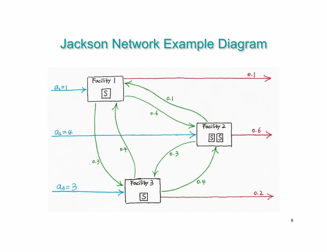
Jackson Network Example Diagram

9

Jackson Network Example (cont’d)

•  Plugging into the formula for λj for j = 1, 2, 3, we obtain

•  The simultaneous solution for this system is

10

!1 =1 + 0.1!2 + 0.4!3!2 = 4+ 0.6!1 + 0.4!3!3 = 3+ 0.3!1 + 0.3!2

!1 = 5, !2 =10, !3 = 712

Jackson Network Excel Template

11

Jackson Network Example (cont’d)

•  Given this simultaneous solution for λj, to obtain the distribution of the number of customers Ni = ni at facility i, note that

12

!i ="isiµi

=

12

for i =1

12

for i = 2

34

for i = 3

!

"

###

$

###

Pn2=

13

for n2 = 0

13

for n2 =1

13

12!

"#$

%&n2'1

for n2 ( 2

)

*

++++

,

++++

for facility 2,

Pn1=

12

12!

"#$

%&n1

for facility 1,

Pn3=

14

34!

"#$

%&n3

for facility 3.

Jackson Network Example (cont’d)

•  The joint probability of (n1, n2, n3) then is given simply by the product form solution

•  The expected number of customers Li at facility i

•  The expected total number of customers in the system

13

P (N1,N2,N3) = (n1,n2,n3){ }= Pn1Pn2Pn3

L1 =1, L2 =43, L3 = 3

L = L1 + L2 + L3 = 513

Jackson Network Example (cont’d)

•  To obtain W, the expected total waiting time in the

system (including service times) for a customer, you

cannot simply add the expected waiting times at the

respective facilities, because a customer does not

necessarily visit each facility exactly once.

•  However, Little’s formula can still be used for the entire

network,

14

W =L

a1 + a2 + a3=16 / 31+ 4+3

=23