Prospect Theory or Skill Signaling?

Rick Harbaugh∗

Abstract

Failure is embarrassing. In gambles involving both skill and chance, we show that a strategic

desire to avoid appearing unskilled generates behavioral anomalies consistent with prospect

theory’s concepts of loss aversion, framing effects, and probability weighting. Based on models

from the career concerns literature that formalize early social psychology models of risk taking,

the results show that skill signaling and prospect theory behavior might be confounded in

economic, financial, and managerial decisions where both skill and chance are important. We

identify specific situations where skill signaling makes opposite predictions than prospect theory,

allowing for tests between the strategic and behavioral approaches to understanding risk. D81;

D82; C92; G11

Most risky decisions involve both skill and chance. Success is therefore doubly fortunate in that

it brings both material gain and an enhanced reputation for skill, while failure is doubly unfortunate.

Often the reputational effects are more important than the direct material gain or loss. For instance,

the manager of a successful project wins the confidence of superiors to oversee more projects, while

the manager of a failed project is viewed as incompetent and loses future opportunities. In other

cases the reputational effects are less important but still of some concern. For instance, an investor

who picks a successful stock enjoys the esteem of friends and family, while an investor who chooses

poorly looks like a foolish loser.

The idea that decision makers choose between risky actions to limit the embarrassment of failure

is emphasized in the early social psychology literature on achievement motivation (John Atkinson,

1957), and similar ideas appear in the literatures on self-esteem (Henry James, 1890) and self-

handicapping (Edward Jones and Steven Berglas, 1978). These literatures assume that failure

reflects unfavorably on perceived skill without analyzing the exact information flows. The literature

on the career concerns of managers analyzes more formally how skill and chance affect Bayesian

updating of a manager’s skill, and shows that the incentive to avoid looking unskilled can explain

seemingly irrational behaviors by managers (Bengt Holmstrom, 1982).

∗Kelley School of Business, Indiana University, Bloomington, IN (email: riharbau@indiana.edu). I thank David

Bell, Roland Benabou, Tom Borcherding, Bill Harbaugh, Ron Harstad, Tatiana Kornienko, David Laibson, Ricky

Lam, Harold Mulherin, Jack Ochs, Al Roth, Lan Zhang, and seminar participants at the Claremont Colleges, De-

Paul University, Emory University, IUPUI, Princeton University, UNC/Duke, University of Missouri, the Behavioral

Research Council, the Econometric Society Winter Meetings, the Stony Brook Game Theory Conference and the

Midwest Theory Meetings.

1

In this paper we use the formal approach of the career concerns literature to reexamine the role

of embarrassment and loss of self-image in standard problems involving decision under risk. The

results provide formal support for the principal insights of the early social psychology literatures and

extend these insights in novel ways. Moreover, we show a close connection between these approaches

which are consistent with expected utility maximization, and the non-expected utility approach of

prospect theory (Daniel Kahneman and Amos Tversky, 1979; Amos Tversky and Daniel Kahneman,

1992). We concentrate on identifying what violations of expected utility will appear to arise if a

rational decision maker is concerned with appearing skilled, but is instead modeled as only caring

about immediate monetary payoffs.

We show that skill signaling leads to behavior consistent with prospect theory’s concepts of loss

aversion, framing effects, and probability weighting.1 Loss aversion refers to the utility function

having a kink at the status quo wealth level so that utility falls more steeply in losses than it rises

in gains (Kahneman and Tversky, 1979). Gambles with small stakes can therefore have substantial

risk premia even though a standard smooth utility function would predict near risk neutrality (John

Pratt, 1964; Matthew Rabin, 2000). Framing refers to how the presentation of a gamble relative to a

reference point can change behavior. It predicts risk aversion when the outcomes are presented as a

gain relative to a reference point, and risk lovingness when the same outcomes are presented as a loss

relative to the reference point (Tversky and Kahneman, 1981). Finally, probability weighting refers

to the idea that decision makers violate expected utility theory by overweighting low probabilities

(Kahneman and Tversky, 1979; Tversky and Kahneman, 1992). It can explain the simultaneous

purchase of lottery tickets and insurance (Milton Friedman and L.J. Savage, 1948), the Allais paradox

(M. Allais, 1953), and the preference for “long shots” by gamblers (Richard Thaler and William

Ziemba, 1988).

To analyze the role of skill signaling, we follow the career concerns literature in investigating

two types of skill. First, with “performance skill” some decision makers face better odds of success,

i.e., a project is more likely to succeed under a skilled manager. Performance skill has been used to

understand “rat race” career incentives (Holmstrom, 1982), excessive risk-taking (Bengt Holmstrom

and Joan Costa, 1986), and corporate conformism (Jeffrey Zwiebel, 1995). Second, with “evaluation

skill” some decision makers are better at identifying the exact odds of a gamble, i.e., a skilled manager

chooses more promising projects, or a skilled broker identifies more profitable companies. Evaluation

skill has been used to understand distorted investment decisions (Holmstrom, 1982), herding (David

Scharfstein and Jeremy Stein, 1990), anti-herding (Christopher Avery and Judith Chevalier, 1999),

the sunk cost fallacy (Chandra Kanodia, Robert Bushman, and John Dickhaut, 1989), conservatism

and overconfidence (Canice Prendergast and Lars Stole, 1996), and political correctness (Stephen

Morris, 2001).

We differ from most of the career concerns literature in that we do not explicitly model the

1These concepts were originally identified from laboratory experiments, but prospect theory has since been applied

widely to analyze economic and financial environments where the role of skill has been emphasized in the career

concerns literature (Colin Camerer 2000, Nicholas Barberis and Richard Thaler 2001).

2

details of the career environment. Instead we derive general results for situations where individuals

are “embarrassment averse” in the same pattern as is normally assumed for risk aversion regarding

wealth. That is, their utility is increasing in their expected skill, and they particularly dislike being

thought of as unskilled. Such a pattern could reflect a simple desire to avoid embarrassment or

maintain one’s own self-image. Or, from a career concerns perspective, the pattern arises if future

income is a linear function of estimated skill and people are risk averse with respect to wealth. It can

also arise if expected future income is a concave function of estimated skill because, for instance, the

probability of maintaining employment is a concave function of performance (Judith Chevalier and

Glenn Ellison, 1999). Our reduced form approach allows the results to be applied to any environment

that generates future income based on success or failure in a pattern consistent with the general

conditions of embarrassment aversion.

To see how skill signaling leads to similar predictions as prospect theory, first consider loss

aversion. When there is a performance skill component to a gamble, losing implies that there is

a good chance that the decision maker bungled the gamble, and when there is an evaluation skill

component, losing implies that the decision maker might have unwisely taken a gamble that had

worse than expected odds. In either case, losing reflects poorly on the decision maker’s skill, so if

the decision maker is risk averse with respect to skill estimates, then she is more averse to gambling

than pure risk aversion regarding monetary payoffs would predict. Since losing even a “friendly bet”

with no money at stake is embarrassing, this effect does not disappear as the stakes of the gamble

become smaller,2 so the utility function in wealth will appear to be kinked at the status quo, i.e.,

the decision maker will appear to be loss averse.

Regarding framing, multiple equilibria often exist depending on whether the observer expects the

decision maker to gamble or not, and depending on what the observer believes about the decision

maker’s skill if she takes a different choice. Therefore the decision maker might use the framing

of the gamble to better understand the observer’s expectations. Depending on whether refusal to

take a gamble is interpreted as an admission of being unskilled, even an unskilled decision maker

might be “dared” into gambling. If losing is portrayed as the reference point then taking a fixed sum

instead of the gamble is an improvement over the reference point, so refusing the gamble is unlikely

to be viewed negatively. But if winning is portrayed as the reference point, then taking a fixed sum

instead of the gamble is worse than the reference point, so the decision maker has reason to expect

that refusing the gamble will be viewed as an admission of being unskilled. These beliefs imply that

gambling is less likely in the former case than the latter case as predicted by prospect theory.3

2This is consistent with Robert Schlaifer’s (1969, p.161) suggestion that in some cases “nonmonetary consequences”

of losing may explain high risk premia for small gambles.3The existence of multiple equilibria also implies a role for cultural factors. For instance, it is documented that

men take riskier investments than women do (Nancy Jianakoplos and Alexandra Bernasek, 1998), invest as if they are

overconfident (Brad Barber and Terrance Odean, 2001), and generally appear to be less risk averse (Catherine Eckel

and Phillip Grossman, forthcoming; Rachel Croson and Uri Gneezy, 2004). If observers expect men but not women

to take risky actions, then the negative inference from not taking a gamble is larger for men, so the beliefs can be

self-fulfilling.

3

Regarding probability weighting, prospect theory finds that decision-makers exhibit a “four-fold

pattern” of behavior in which they tend to favor long-shots but also avoid near sure things, and to

buy insurance to protect against unlikely losses even as they will take risky chances to win back

large losses.4 To capture this observed pattern, probability weighting as developed most fully in

“cumulative prospect theory” (Tversky and Kahneman, 1992; Prelec, 1998) assumes that people

violate expected utility maximization by overweighting small probability gains (such as taking a

10% chance of winning $100 over $10 for sure) and underweighting high probability gains (such as

taking $90 for sure over a 90% chance of winning $100), and by overweighting low probability losses

(such as paying $10 for sure rather than risking a 10% chance of losing $100), and underweighting

high probability losses (such as risking a 90% chance of losing $100 rather than paying $90 for sure).

From the perspective of skill signaling, the four-fold pattern can be interpreted more simply as

overweighting of small probabilities of success (e.g., favoring long shots and taking chances to win

back large losses) and underweighting of high probabilities of success (e.g., avoiding near sure things

and buying insurance). For either performance or evaluation skill, we find that losing a gamble

that is known to have a low probability of success is less embarrassing than losing a gamble where

success is expected, so lower probability gambles are favored. When success is unlikely, failure is

common but only slightly reduces the perceived skillfulness of the decision maker because both

skilled and unskilled decision makers usually fail. But when success is likely, failure is rare but

far more embarrassing because a person who fails is probably unskilled. Embarrassment averse

decision makers are therefore more willing to take gambles that observers recognize are long shots,

and reluctant to take gambles where success is expected.

For gambles involving performance skill, the preference for long shots is strengthened if the

decision maker has private information about her own skill. Failure to take a gamble can then be

seen as lack of confidence, so the decision maker faces pressure to risk failure rather than directly

admit her incompetence by refusing to gamble. Since long shots offer little embarrassment from

losing, the gamble is worth taking if the expected monetary return is not too negative. For gambles

involving evaluation skill, the preference for long shots is strengthened if the outcome of a refused

gamble is still observable so the decision maker cannot prevent the observer from learning about her

skill. If the gamble is refused, a good outcome is a strong indication that the decision maker failed

to recognize that the gamble had better than expected odds. For long shots this possibility is more

embarrassing than taking the gamble and losing, so the decision maker will take the gamble if the

expected monetary return is not too negative.

These results indicate that the behavioral approach of prospect theory and the strategic approach

of skill signaling can provide very similar predictions in economic and financial environments where

the career concerns literature has shown a strong role for skill signaling. This overlap can be seen

4“Original prospect theory” (Kahneman and Tversky, 1979) assumes that the utility function is convex in losses

and concave in gains, implying the simpler pattern that decision makers are risk loving in gambles that involve

potential losses and risk averse in gambles that involve potential gains. Applications of prospect theory often allow

for interactions between both patterns, but in this paper we concentrate on the four-fold pattern.

4

as mutually reinforcing — the theoretical results of skill signaling provide an underlying strategic

foundation for the behavioral predictions of prospect theory, and the empirical results of prospect

theory indicate that decision makers are capable of understanding and even internalizing the logic

of skill signaling. To see when the predictions of prospect theory and skill signaling diverge, we

consider an extension of the model where the probability of the gamble is not observable to others.

In this we case we find that the decision maker prefers high probability rather than low probability

gambles, in contrast with the predictions of prospect theory.

In the following section we provide an introductory example, and then in Section II we develop

a more formal model which considers the existence of multiple equilibria and provides results in

terms of risk premia. Section III relates the results in more detail to prospect theory and to other

models including achievement motivation, self-esteem, self-handicapping, disappointment aversion,

and regret theory. Section IV concludes the paper.

1 Introductory Example

Consider a gamble with two outcomes, “win” or “lose”, taken by a decision maker who is either

skilled “s” or unskilled “u”. For this example we consider the simplest case of performance skill

where the decision maker does not have any private information about her own skill so that the act

of taking a gamble is not itself informative of skill. The probability of being skilled conditional on

winning is therefore

Pr[|] =Pr[ ]

Pr[]= Pr[] +

Pr[ ]− Pr[] Pr[]Pr[]

(1)

= Pr[] +Pr[ ]− Pr[] Pr[ ]− Pr[] Pr[ ]

Pr[]

= Pr[] +Pr[|]− Pr[|]

Pr[]Pr[] Pr[]

Similarly, the probability of being skilled conditional on losing is

Pr[|] = Pr[]− Pr[|]− Pr[|]Pr[]

Pr[] Pr[] (2)

Assuming that the “skill gap” Pr[|] − Pr[|] = Pr[|] − Pr[|] is positive, the priorskill estimate Pr[] is updated favorably when the decision maker wins and unfavorably when the

decision maker loses, and the updating is stronger the larger is the skill gap and the weaker is the

prior skill estimate, i.e., the closer are Pr[] and Pr[] to 12.

To see how such updating can affect behavior, suppose that the decision maker’s utility is a

function of both wealth and of her estimated skill by an observer, who could be the decision maker

herself if self-esteem is important.5 Assuming that the two components of utility are additively

separable and letting represent the skill estimate component, if is concave then the decision maker

prefers the prior skill estimate Pr[] rather than risk the lower estimate Pr[|]. In particular,5As discussed in Section 4, Roland Benabou and Jean Tirole (2002) analyze how self-esteem can affect behavior.

5

since Pr[] Pr[|] + Pr[] Pr[|] = Pr[] by the law of iterated expectations, Jensen’s

inequality implies that

(Pr[]) Pr[](Pr[|]) + Pr[](Pr[|]) (3)

for 00 0, so a decision maker is more wary of gambles than pure monetary considerations would

suggest. As the monetary size of the gamble becomes smaller, risk aversion with respect to the

monetary component of utility should asymptotically disappear for a smooth utility function, but

the fear of looking unskilled remains even for a “friendly bet” with no money at stake.6 Therefore,

the concept of loss aversion can be consistent with a standard smooth utility function.7

Now consider how the decision maker’s attitude toward a gamble is affected by the odds of the

gamble. From (1) and (2), for a given skill gap Pr[|]−Pr[|], both Pr[|] and Pr[|]are decreasing in Pr[], so the higher is Pr[], the weaker is the favorable updating and the

stronger is the unfavorable updating. Therefore, when a gamble is a long shot the decision maker

has little to fear from losing and a lot to gain from winning. And when a gamble is a near sure thing

the decision maker has little to gain and a lot to lose. More generally, if the skill gap depends on

Pr[], as is necessary to keep Pr[|] and Pr[|] bounded in [0,1] as Pr[] approaches 0or 1, these updating patterns hold as long as the skill gap does not change too rapidly as Pr[]

rises.8

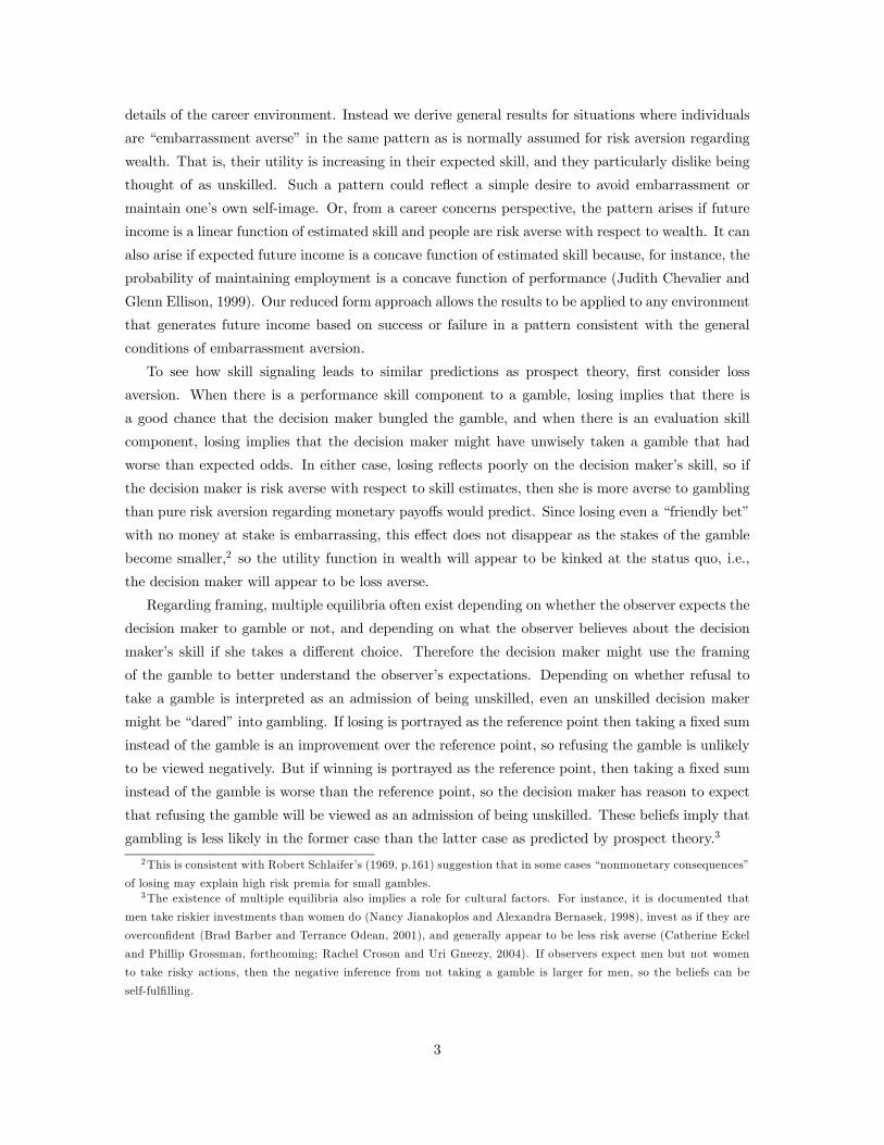
Figure 1(a) shows the updated skill estimates when the prior is Pr[] = 12 and the skill gap

for any gamble takes the form Pr[|]− Pr[|] = 2Pr[] Pr[]. This simple formulationensures that Pr[|] 1 and Pr[|] 0 as Pr[] approaches 1 or 0 and is symmetric

in that the skill gap is the same for a gamble with probability Pr[] = and a gamble with

probability Pr[] = 1− .9 As we will see in Section 3, this formulation is implicitly assumed by

the achievement motivation literature. When Pr[] is low, winning has a large impact on estimated

skill as seen from the divergence of the top line Pr[|] from the prior Pr[] = 12, while losing hasonly a small impact as seen from the closeness of the bottom line Pr[|] to expected skill. Lowprobability gambles therefore present a chance of standing out with little downside risk. Conversely,

when Pr[] is high, winning has only a small impact on estimated skill whereas losing has a large

impact. Such gambles offer little opportunity to prove the sender’s skill but carry substantial danger

of embarrassment.

6The skill gap itself might shrink as the size of the gamble shrinks because the decision maker cares less about the

outcome, e.g., the decision maker might allocate resources to performing at or evaluating gambles depending on their

size (Mathias Dewatripont, Ian Jewitt and Jean Tirole, 1999; Todd Milbourn, Richard Shockley, and Anjan Thakor,

2001). However, given a concern for appearing skilled, there is no reason to assume that the skill gap should go to

zero.7Reputational risk appears in various contexts in the career concerns literature starting with Holmstrom

(1982/1999), but the connection with loss aversion does not appear to have been noted previously.8From (1) and (2) the patterns hold if (Pr[|]− Pr[|]) Pr[] is decreasing in Pr[] and

(Pr[|]− Pr[|]) (1− Pr[]) is increasing in Pr[].9As long as the skill gap has the form Pr[|] − Pr[|] = Pr[] Pr[] for ∈ [0 2] the posterior skill

estimates are linear in Pr[] and bounded in [0 1] as seen in Figure 1(a).

6

Figure 1: Impact of winning and losing on estimated skill and expected utility

The prospect theory literature finds that decision makers tend to be more wary of near sure things

relative to long shots, which is consistent with this pattern that losing is more embarrassing for high

probability gambles. However, even though losing at a near sure thing implies severe embarrassment,

losing occurs only rarely, so it is not immediately clear whether decision makers will be more averse

to such gambles. Figure 1(b) shows this tradeoff for a constant relative risk aversion function

() = −1.10 As seen in the figure, the expected skill estimate from the long shot (Pr[] = 2)

is a weighted average of = Pr2[|] and = Pr2[|], while the expected skill estimate fromthe near sure thing (Pr[] = 8) is a weighted average of = Pr8[|] and = Pr8[|], withthe pattern . Since 000 0, i.e., there is “downside risk aversion” (Whitmore, 1970)

as is usually assumed for risk aversion with respect to monetary outcomes,11 the embarrassment

from losing at a near sure thing is so large that the long shot offers higher expected utility for the

non-monetary component of utility, 2() + 8() 8( ) + 2().12

To see this, 000 0 implies that the slope of is decreasing at an increasing rate from [ ] to

[ ] to [], so the average slope is steeper over the whole range [] than over the middle range

10For a CRRA function () = 1−(1 − ) the coefficient of relative risk aversion, = −000, is = 2 in

this example. Typical estimates of for risk aversion regarding wealth, which may be confounded by embarrassment

aversion, range from = 2 upwards.11For 0 0 and 00 0, decreasing absolute risk aversion (including the standard case of constant relative risk

aversion) requires 000 0. Decreasing absolute risk aversion implies that demand for risky assets increases with

wealth (Pratt, 1964) and that consumers engage in precautionary savings (Miles Kimball, 1990).12Whitmore (1970) shows that if distribution third order stochastically dominates , as can be shown to hold in

this example, then it offers higher expected utility for the class of utility functions satisfying 0 0, 00 0, and

000 0. C. Menezes, C. Geiss, and J. Tressler (1980) show that is preferred to for the larger class satisfying

000 0 if is a mean and variance preserving transformation of , as is true in this example but not in our more

general model.

7

[ ], i.e., (()− ())(−) (( )− ())( − ).13 For a symmetric pair of gambles like

this one where is the probability of winning at the long shot and 1− is the probability of winningat the near sure thing, +(1−) = [] = (1−)+ and hence (−) = (1−)(−), thisimplies that (()− ()) (( )− ())(1− ), or () + (1− )() (1− )( ) + ().

Therefore, separate from the monetary returns, the long shot offers higher expected utility. As

we discuss in Section 3, this application of downside risk aversion may provide an expected utility

basis for the probability weighting phenomenon identified in the prospect theory literature, and also

provides formal support for basic insights behind the achievement motivation and self-handicapping

literatures.

In the following section we allow the decision maker to have some private information about her

own ability and/or about the gamble itself. We show that the tendency to favor low probability

gambles continues to hold, and is strengthened by two effects. First, when the decision maker has

private information about her ability, refusing to take a gamble can reveal a lack of confidence.

Therefore, for a long shot where the embarrassment from losing is small, gambling can be attractive

even if there is a negative expected monetary return. Second, when the decision maker has private

information about the gamble, rejecting a gamble that ultimately succeeds reflects unfavorably on

the decision maker’s judgement. For a long shot this is more dangerous than gambling and losing,

so again it can be worthwhile to take a chance on a long shot with a negative expected monetary

return.

2 The Model

We analyze a generalization of the above example that allows for both performance skill and evalua-

tion skill. A decision maker of skill ∈ faces a gamble with payoff ∈ ⊂ R where (“losing” or “failure”) is strictly less than (“winning” or “success”). The decision maker

learns an unverifiable private signal ∈ and then accepts or rejects the gamble. An observerthen observes the decision and the outcome of the gamble if it is accepted. The observer’s only role

is to estimate the decision maker’s skill given all available information Ω. To simplify the presenta-

tion we normalize skill type = 0 and = 1 so that [|Ω] = Pr[|Ω]. The decision maker’s utilityis a quasilinear function of wealth and her estimated skill by the observer, = + (Pr[|Ω])where is thrice-differentiable on (0 1).14

We assume that a “skilled” decision maker is more likely to win than an “unskilled” one,

Pr[|] ≥ Pr[|] , and that a “good” signal indicates a higher probability of winning thana “bad” signal, Pr[|] Pr[|]. We say there is pure performance skill if the first inequalityholds strictly, Pr[|] Pr[|], and is a signal about the decision maker’s own skill that

13This is shown as part of Lemma 1 for this example where − = − .14The quasilinearity assumption allows the effect of embarrassment aversion on risk premia to be isolated. The

utility function should be locally linear in wealth (Pratt, 1964), so this simplification is more appropriate for smaller

gambles.

8

provides no additional information on winning conditional on skill, Pr[| ] = Pr[|]. Wesay there is pure evaluation skill if the first inequality holds weakly, Pr[|] = Pr[|], and

is instead a signal of the gamble’s likely success that is more informative for a more skilled decision

maker, Pr[| ] − Pr[| ] Pr[| ] − Pr[| ]. To allow for both types of skill

separately or together we assume that Pr[| ] Pr[| ] and Pr[| ] − Pr[| ] ≥Pr[| ]−Pr[| ]. To ensure that there is always some noise, we also assume that the jointdistribution ( ) has full support.

Our equilibrium concept is perfect Bayesian equilibrium with D1-proof beliefs (In-Koo Cho and

David Kreps, 1987). Therefore Pr[|Ω] is based on Bayes’ Rule for play on the equilibrium path, andthe observer believes any deviation from the equilibrium path is by the type who benefits from such

a deviation for the largest range of responses by the observer. We will show that the D1 refinement

implies the natural restriction on beliefs that if a decision maker unexpectedly gambles then the

observer believes that she has good news ( = ), and that if a decision maker unexpectedly does

not gamble then the observer believes that she has bad news ( = ).15 Because the signal to gamble

or not is binary, D1 does not imply a unique equilibrium.

We restrict our attention to pure strategy equilibria. First consider a separating equilibrium

in which a decision maker with good news gambles and a decision maker with bad news does

not. Generalizing (1) and (2), if a gamble is accepted the expected skill conditional on and the

equilibrium belief that = is

Pr[| ] = Pr[|] + Pr[| ]− Pr[| ]Pr[|] Pr[|] Pr[|] (4)

and if a gamble is rejected the expected skill given the equilibrium belief that = is just Pr[|].The payoff for type from gambling is therefore [|]+[(Pr[| ])|], where [(Pr[| ])|] =Pr[|](Pr[| ])+ Pr[|](Pr[| ]), and the payoff from not gambling is (Pr[|]).For the candidate equilibrium to exist, it must be that for a type the net financial reward from

taking a chance and gambling is less than the net skill estimate benefit from playing it safe and not

gambling,

[|] (Pr[|])−[(Pr[| ])|] (5)

and that the opposite is true for a type,

[|] ≥ (Pr[|])−[(Pr[| ])|] (6)

Since [|] and Pr[|] are increasing in and Pr[| ] Pr[| ], for 0 0 there alwaysexists a gamble with intermediate monetary payoffs that satisfies these conditions.

In the separating equilibrium a type with good news “shows off” by gambling, but when evalua-

tion skill is sufficiently important relative to performance skill and when the financial costs to losing

15Divinity (Jeffrey Banks and Joel Sobel, 1987) implies the weaker restriction that the observer puts more weight on

the decision maker having good (bad) news in the former (latter) case, while the intuitive criterion (Cho and Kreps,

1987) need not restrict beliefs in our context. As shown in an earlier version of this paper, these weaker restrictions on

beliefs generate similar behavioral predictions as D1, though the lack of unique beliefs complicates the presentation.

9

are sufficiently small, a “reverse separating” equilibrium might be possible. In this case a decision

maker with a bad rather than good signal is expected to gamble, so that losing rather than winning

is a positive sign of having an accurate signal. Since this equilibrium seems comparatively unlikely,

to simplify the presentation we rule it out by assuming that the financial costs of such behavior

outweigh any reputational gains from appearing skilled,16

[|] +[(Pr[| ])|] [|] +[(Pr[| ])|] (7)

or, simplifying,

− (Pr[| ])− (Pr[| ]) (8)

Since by assumption, and since losing is never a good sign for a pure performance skill

gamble, Pr[| ] − Pr[| ] = Pr[|] − Pr[|] 0, this assumption is only relevant if

there is an evaluation skill component to the gamble.

For pooling equilibria, the two possibilities are a both-gamble equilibrium and a neither-gamble

equilibrium. In the both-gamble equilibrium, the observer cannot condition on so expected quality

from accepting the gamble is just Pr[|] as defined in (1) and (2). If the gamble is unexpectedlyrefused then, as we confirm in the proof of Proposition 1, the D1 refinement implies that the observer

believes that the decision maker has a signal, so the expected quality is just Pr[|]. Therefore thecondition for existence of a both-gamble equilibrium is, for = ,

[|] ≥ (Pr[|])−[(Pr[|])|] (9)

which clearly holds for a sufficiently high monetary payoff for the gamble.

Regarding the neither-gamble equilibrium, the expected quality from not gambling is just Pr[]

and the expected quality from gambling depends on the observer’s beliefs about who would unex-

pectedly gamble. As we confirm in the proof of Proposition 1, the D1 refinement implies in this

case that the observer believes that the decision maker has a signal, so the expected quality is

Pr[| ]. Therefore the condition for a neither-gamble equilibrium is, for = ,

[|] (Pr[])−[(Pr[| ])|] (10)

which clearly holds for a sufficiently low monetary payoff for the gamble.

These conditions are summarized in the following proposition. The details of the proof regarding

the D1 refinement are in the Appendix, as are all subsequent proofs.

Proposition 1 Suppose 0 0. The separating equilibrium exists iff (5) and (6) hold, the both-

gamble equilibrium exists iff (9) holds, and the neither-gamble equilibrium exists iff (10) holds.

Since utility is linear in wealth, the risk premium in our model just equals the net loss or gain

from the skill estimate component of expected utility. For the introductory example without private

16This assumption also simplifies analysis of beliefs for the neither-gamble equilibrium in the proof of Proposition

1.

10

information in Section I, the risk premium is (Pr[])−(Pr[](Pr[|])+Pr[](Pr[|])),so the risk premia for the Pr[] = 2 and Pr[] = 8 gambles are the vertical distances in Figure

1(b) between (Pr[]) and the expected utilities of the gambles.17 Allowing for private information,

the risk premia will depend both on this information and on the equilibrium being played. In

particular, for the separating equilibrium the risk premium for type , denoted by , is the RHS of

(5), and the risk premium for type , denoted by , is just the RHS of (6). Similarly, the risk premia

for the both-gamble and neither-gamble equilibria are given by the RHS of (9) and (10) respectively.

When we do not distinguish risk premia by type we refer to their average, = Pr[] + Pr[],

as the risk premium.

The risk premium is always positive in gambles without skill signaling when utility is concave

in wealth (Pratt, 1964), and this is also true for concave in the introductory example without

private information. But when we allow for private information, refusal to gamble can signal lack

of confidence as seen by the role of in the conditions (5), (6), (9) and (10), so the decision maker

has an added incentive to gamble, implying that risk premia can be negative rather than positive. If

the risk premium is positive (negative) then there is an expected loss (gain) to the skill estimate

component of utility from taking the gamble, so the expected monetary payoff [|] that wouldmake type indifferent is greater (less) than zero. Since the sign of the risk premium gives a simple

indication of whether a “fair gamble” with [|] = 0 will be accepted or rejected by type , it

provides a summary measure of whether skill signaling leads to more or less risky behavior. The

risk premia also provide a basis for relating our results to non-expected utility models of probability

weighting as we discuss in Section 3.

The following two propositions provide conditions under which the tradeoff between admitting

incompetence by not gambling and risking embarrassment by gambling can be signed, so that the

risk premia are definitely positive or negative. The first one considers the case where the gamble has

some performance skill Pr[|] Pr[|]. If the probability of winning is small enough then thereis little loss in estimated skill from losing, so the decision maker is better off taking a fair gamble

than admitting to having a bad signal. Conversely, if this signal is very informative, Pr[|]−Pr[|]approaches 1, then the amount of bad information provided by choosing to not gamble dominates

any risk from gambling even when losing is very embarrassing, so the decision maker is better off

gambling. This captures the idea that people can be dared into taking a gamble. For instance,

teenagers might “overconfidently” take risky actions to prove that they are not afraid. Even if they

are not skilled at the risky activity they may prefer to give in to peer pressure and take a chance

rather than confirm their inadequacy through refusing the dare.

Proposition 2 Suppose 0 0. In any pure strategy equilibrium the risk premium is negative

for a) any given Pr[|]− Pr[|] 0 and sufficiently low Pr[|], or b) any given Pr[|] andsufficiently large Pr[|]− Pr[|].

The next proposition considers the opposite case where Pr[|]−Pr[|] is small, e.g., the decision17For () = −1 the risk premium is 2Pr[](2− Pr[]), so it is six times higher for the latter gamble.

11

maker has very little private information about the odds of success as in the introductory example,

or this information is uncorrelated with skill, Pr[|] = Pr[|], as in a pure evaluation skill gamble.In this case very little information about ability is revealed by refusing to gamble, so for 00 0 the

decision maker prefers to not gamble rather than risk embarrassment.18 19

Proposition 3 Suppose 00 0. In any pure strategy equilibrium the risk premium is positive for

any given Pr[|] and sufficiently small Pr[|]− Pr[|].

Comparing conditions (9) and (10), the both-gamble and neither-gamble equilibrium can coexist

depending on the parameter values, and comparing conditions (6) and (10), the separating and

neither-gamble equilibria always coexist for some monetary payoffs of the gamble [|]. The riskpremia in each equilibrium are different so the incentive to gamble or not depends in part on

what equilibrium is expected. For instance, not gambling is not penalized in the neither-gamble

equilibrium while it is in the separating and both-gamble equilibria, so the risk premium (positive

or negative) necessary to induce gambling is higher in the neither-gamble equilibrium.

When multiple equilibria exist the “framing” of the gamble can potentially make a difference in

determining whether a decision maker gambles or not. In particular, if the framing leads the decision

maker to expect the observer to have a negative impression of those who do not gamble, then the

decision maker is more likely to gamble, e.g., the both-gamble or separating equilibrium is more likely

than the neither-gamble equilibrium. Prospect theory finds that the “reference point” of a gamble

can affect behavior, in that gambles are more likely when the fixed alternative to gambling is framed

as being below the reference point. In a skill signaling model, manipulating the reference point can

be seen as providing information to the decision maker about how gambling or not gambling will

be perceived, and a high reference point could indicate that failure to gamble will be interpreted

negatively by the observer.

The finding from Proposition 2 that sufficiently low probability gambles have a negative risk

premium is consistent with the tendency to favor low probability gambles that is found in the

prospect theory and related literatures. A related result was found in the introductory example

where it was shown that a decision maker prefers a fair gamble with a 20% chance of winning to

a fair gamble with an 80% chance of winning. To investigate this issue of favoring low probability

gambles more generally, we now compare risk premia for pairs of gambles where, as in the example,

the probability of winning at one gamble is equal to the probability of losing at the other gamble.

The current environment is more complicated in that we must hold constant any differences in

private information by the decision maker about her skill and/or the gamble. We refer to a pair of

gambles as symmetric if the probability of winning at one gamble equals the probability of losing

18Tyler Cowen and Amihai Glazer (2007) consider labor market applications where decision makers are likely to

be risk averse with respect to estimates of their ability and therefore prefer to keep observers ignorant of their exact

ability.19 In some contexts might be convex, e.g., when a higher performance evaluation will ensure a promotion but a

lower evaluation will not lead to a demotion. Similar issues arise regarding reversal of the standard assumption of

risk aversion with respect to wealth, e.g., when higher wealth allows purchase of a large indivisible good.

12

at the other, if the skill gap is the same, and if the probability of being skilled given the decision

maker’s signal is the same. To simplify the comparison we also assume that the probabilities of a

good and bad signal are the same.

Definition 1 Gambles and are a symmetric pair if [] = [], Pr [] = Pr[],

Pr [| ] −Pr [| ] = Pr[| ] − Pr[| ], Pr [|] = Pr[|], and Pr [] =Pr[] = 12 for ∈ , ∈ .

Using this definition, the first part of the following proposition shows that embarrassment aversion

implies lower risk premia on low probability gambles than on high probability gambles in each of the

pure strategy equilibria. The second part then shows that, if we consider gambles with equivalent

expected payoffs, e.g., a gamble with a 20% chance of winning $100 is priced at $20 and a gamble

with an 80% chance of winning $100 is priced at $80, the both-gamble equilibrium is more likely

for low probability gambles and the neither-gamble equilibrium is more likely for high probability

gambles.

Proposition 4 Suppose 0 0, 00 0, and 000 0 and consider a symmetric pair of gambles

and with Pr [] Pr[]. (i) In any given pure strategy equilibrium the risk premium

is lower for than for . (ii) A both-gamble equilibrium exists for if it exists for , and a

neither-gamble equilibrium exists for if it exists for .

This result provides the straightforward prediction that, for equal expected monetary payoffs,

sufficiently low probability gambles are more frequently taken than sufficiently high probability

gambles. Since measuring exact risk premia requires measuring willingness to pay, and since the

decision maker has an incentive to strategically manipulate such information, this substantially

simplifies testing the model.20

2.1 Extension: Outcome observed even if gamble refused

So far we have assumed that if the gamble is refused the observer does not learn the outcome of the

gamble. But often the outcome is observable anyway, e.g., the price of a publicly traded asset rises

or falls regardless of whether a particular decision maker buys it or not. In such cases the decision

maker will be evaluated based on the outcome whether she takes the gamble or not, e.g., purchasing

a stock that does poorly indicates poor skill at evaluating stocks, but so does not purchasing a

stock that does well. Since no information is revealed about skill if a gamble that only involves

performance skill is refused, we are interested in gambles with an evaluation skill component. For

simplicity we restrict attention to the case of pure evaluation skill.

If a decision maker is expected to gamble if and only if she has good news about the probability

of success, i.e., there is a separating equilibrium, then the decision maker looks wise for refusing a

20 In our model there is the usual incentive to underestimate willingness to pay so as to avoid paying too much, and

also a potential incentive to overestimate willingness to pay so as to signal private information about skill.

13

gamble that loses and looks foolish for refusing a gamble that wins. Therefore the updating process

works in the opposite direction as with accepted gambles. This is most clear when a gamble is

symmetric.

Definition 2 Gamble with pure evaluation skill is symmetric if Pr[| ] −Pr[| ] =Pr[| ] −Pr[| ] and Pr[] = Pr[] = 12.

Consider a symmetric gamble with pure evaluation skill where a separating equilibrium is being

played and the gamble is refused. The observer expects the decision maker has a bad signal = ,

so the expected skill conditional on is, for 6= 0,

Pr[| ] = Pr[] +Pr[| ]− Pr[| ]

Pr[|] Pr[] Pr[] (11)

= Pr[] +Pr[0| ]− Pr[0| ]

Pr[|] Pr[] Pr[]

Looking at the first line of (11), since the gamble is more likely to lose if a decision maker with

a bad signal is skilled, Pr[| ] Pr[| ], refusing a gamble that wins is embarrass-ing, Pr[| ] Pr[]. Considering the second line, for Pr[] 12 symmetry implies that

Pr[|] Pr[|], so Pr[| ] Pr[| ], i.e., it is more embarrassing to refuse a gam-ble that wins than to take a gamble that loses. And for Pr[] 12, the reverse pattern holds,

Pr[| ] Pr[| ]. Therefore, as shown in the first part of the following proposition, gambleswith a low probability of success have negative risk premia even as gambles with a high probability

of success have more standard positive risk premia. For low probability gambles losing is expected

so the negative updating is limited if the gamble is taken and it loses. But for the same reason if

the gamble is refused and it wins, the observer will infer that the decision maker had low quality

information so the negative updating of skill is more substantial. The decision maker therefore has

a reputational incentive to accept a low probability gamble.

In the separating equilibrium the decision maker is judged whether she takes the gamble or

not. But for pooling equilibria where both types take the same action, the decision maker avoids

judgement as long as she does not deviate from the equilibrium. For instance, if both types are

expected to take the gamble, then the success or failure of the gamble provides no information on

the quality of the decision maker’s information and hence on her skill. If the decision maker deviates

and refuses to take the gamble then the observer will, following our D1 refinement, infer that the

decision maker has an unfavorable = signal, so the outcome is informative of the quality of

this signal. Consequently, unless the financial incentives are sufficiently strong, an embarrassment

averse decision maker prefers to stick with the pooling equilibrium. In particular, we find that the

average risk premium is always negative. If we consider the neither-gamble equilibrium then again

it is safer for the decision maker to pool rather than risk standing out and losing, so in this case the

risk premium is always positive.

14

Proposition 5 Suppose 0 0 and 00 0 and the decision maker faces a pure evaluation skill

gamble where the outcome is observed even if the gamble is refused. (i) In the both-gamble (neither-

gamble) equilibrium the risk premium is always negative (positive). (ii) If in addition 000 0 and

the gamble is symmetric then in the separating equilibrium the risk premium is negative (positive)

if Pr[] ()12.

Part (i) implies that for [|] sufficiently close to 0 the both-gamble and neither-gamble equi-libria always coexist since each type of decision maker finds it safest to pool with the other type.

As discussed earlier, this sensitivity of behavior to observer expectations suggests a large role for

framing effects and social influences such as “peer pressure”.

2.2 Extension: Observer uninformed of probability of success

So far we have assumed that the observer knows the unconditional probability of success, Pr[],

but this is not always true, e.g., a manager might know the difficulty of a project, but the manager’s

boss might be in the dark. When the observer is uninformed of the odds of the gamble we would

naturally expect the decision maker to favor high rather than low probability gambles, the opposite

of what we have found so far. Understanding this case helps clarify our main results and also provides

a clear prediction that can separate skill signaling from behavioral models where the decision maker

always favors low probability gambles.

To model this case assume there are two gambles and where Pr [] Pr[] and where

the decision maker faces one of the two gambles, each with positive probability, but the observer does

not know which. If, as we have assumed so far, the decision maker has a private signal for each

gamble that is informative of the probability of success, then the decision maker has two dimensions

of private information so there are a large number of possible separating and partially separating

equilibria. Therefore, for simplicity, we revert to the model in the introduction and assume that the

decision maker does not have any private information other than knowing which gamble is being

faced.

With this assumption, we refer to the separating equilibrium as the equilibrium where the

gamble is taken and the gamble is refused and the both-gamble (neither-gamble) equilibrium as

the equilibrium where either (neither) gamble is taken.

Proposition 6 Suppose 0 0 and the decision maker faces one of two gambles or where

Pr [] Pr[] and there is no private information for either gamble. If the decision maker

knows which gamble she faces but the observer only knows that each gamble is faced with positive

probability, then in any pure strategy equilibrium the risk premium is higher for the gamble than

for the gamble.

This result follows from just reinterpreting our base model with one gamble with private infor-

mation ∈ as a model with two gambles where = corresponds to gamble and =

corresponds to gamble . In our base model the risk premium is always higher for type = , so

15

this implies that the risk premium is higher for gamble . The fact that our base model can be

reinterpreted in this way highlights the importance of being careful in tests of skill signaling. If, for

instance, Pr[|] = 38, Pr[|] = 18, and Pr[] = 14, we predict that the risk premiumis higher for type facing Pr[|] = 18 than for type facing Pr[|] = 38. But we also

predict that the risk premium is lower for each type than in the paired symmetric gamble where

Pr[|] = 58, Pr[|] = 78, and Pr[] = 34. Our main argument in this paper that lowerprobability gambles are favored refers to this latter conclusion.

In addition to these two extensions on observability of refused gambles and observability of the

probability of success, clearly a number of other extensions are possible, many of which appear in

related contexts in the career concerns literature and may also be related to behavioral anomalies.

For instance, the decision maker might be able to choose whether to report that a gamble was taken,

e.g., people often choose whether to inform friends and associates of gambling or stock market

outcomes. In such cases the absence of a report may be interpreted as a sign of failure, thereby

giving an extra incentive to take risky actions. The presence of multiple gambles also changes

the information structure substantially.21 Rather than pursuing more of these extensions we now

consider how our results relate to the literature on behavioral anomalies in risk-taking.

3 Relation to Prospect Theory and Other Models

3.1 Prospect theory

As discussed in the introduction, these results on gambles with a skill component are closely related

to the key phenomena of loss aversion, probability weighting, and framing effects that have been

identified in the prospect theory literature. Since the connections with loss aversion and framing

effects are straightforward, we will concentrate on clarifying the connection between skill signaling

and probability weighting. We are interested in determining what probably weighting function will

be estimated from data on risk taking if the decision maker is concerned in part with looking skilled,

but is modeled as only concerned about the monetary payoffs.22

Our results on risk premia can be related to the probability weighting function by finding the

different certainty equivalents for different values of = Pr[] in a gamble and then inferring what

weighted probability of winning would have induced a risk neutral decision maker unconcerned

with embarrassment aversion (or other factors) to choose that certainty equivalent.23 Setting such

21Multiple gambles are important in the fallacy of large numbers (Paul Samuelson, 1963), the house-money effect

(Richard Thaler and Eric Johnson, 1990), and the disposition effect (Hersh Shefrin and Meir Statman, 1995).22While early social psychology experiments involved real gambles with an explicit skill component, most prospect

theory experiments use hypothetical gambles where it is unclear if subjects perceive a role for skill. Recent exper-

iments using real gambles without a skill component find that probability weighting weakens or disappears (Susan

Laury and Charles Holt, 2008; William Harbaugh, Kate Krause, and Lise Vesterlund, 2002 and forthcoming; Antoni

Bosch-Domenech and Joaquim Silvestre, 2006). Note that loss aversion and framing can also arise without explicit

uncertainty, in which case the role of skill is limited.23Rather than assuming risk neutrality, George Wu and Richard Gonzalez (1996) disentangle the predictions of the

16

that = () + (1− )(), the weighting function is then

=−

− (12)

In our model with embarrassment aversion but without probability weighting the certainty equivalent

is just = () + (1 − )() − . So if the probability weighting function is estimated based

on assuming = without embarrassment aversion, while the true utility function is = +

(Pr[|Ω]) with embarrassment aversion but without probability weighting, then the probabilityweights are estimated as

= −

− (13)

Therefore overweighting is found if the risk premium is negative and underweighting is found if it is

positive, with the amount of reweighting in proportion to the risk premium.24

To see this pattern, first consider the performance skill example from Section I where =

−1Pr[|Ω]. Under the symmetry assumptions Pr[|] − Pr[|] = 2Pr[] Pr[] and

Pr[] = Pr[], risk premia are lower for low probability gambles, so there is more relative weight

on low probability gambles, but still underweighting since risk premia are positive. If in addition

we allow for some private information about skill, then Proposition 2 implies there will be nega-

tive risk premia, and hence probability overweighting, of gambles with sufficiently low probability.

Figure 2(a) shows the imputed probability weighting function for the separating equilibrium where

= 10, = 0, Pr[|]− Pr[|] = 110, and Pr[] = Pr[].25 The general pattern of this

function with its discontinuity at = 0 and = 1 tracks that found in Kahneman and Tversky

(1979).26

Figure 2(b) shows an example of a symmetric pure evaluation skill gamble where the outcome

is observed even if the gamble is refused. We assume a more moderate skill gap, Pr[| ] −Pr[| ] = Pr[| ] − Pr[| ] = Pr[] Pr[], and set = 1 and = 0. The

figure shows the imputed weighting function for the separating equilibrium where, as implied by

Proposition 5, there is overweighting for Pr[] 12 and underweighting for Pr[] 12.

This pattern is similar to that in Tversky and Kahneman (1992), with the exception that they find

underweighting starting at a point below = 12. Recall that behavior in this version of the model

is particularly susceptible to multiple equilibria since both types want to pool with each other when

monetary incentives are weak. In the both-gamble equilibrium the risk premium is always negative

while in the neither-gamble equilibrium it is always positive.

probability weighting function and the convex-concave utility function assumed in original prospect theory.24As discussed in the Introduction, prospect theory treats gambles in gains and losses differently, generating the

“four-fold” pattern of weighting across the two domains. Our model generates this same pattern by considering only

the probability of success, i.e., we do not care about the signs of or but only require that .25The weights are based on the average risk premium for types and . The weights for the both-gamble and

neither-gamble equilibrium are lower since the choice to gamble is less revealing of the decision maker’s private

information.26The discontinuity at = 1 is the “certainty effect” (Kahneman and Tversky, 1979). In our model it arises from

the lack of potential embarrassment, but it can also arise from a fear of being cheated in that it is easier to demand

payment of a certain rather than uncertain amount.

17

Figure 2: Imputed probability weighting functions if skill signaling is omitted, = Pr[]

The parameters in these examples were chosen for their simplicity and their ability to generate

probability weighting functions that track the canonical forms in Kahneman and Tversky (1979)

and Tversky and Kahneman (1992). However, other parameters can generate functions that differ

significantly from these, and the prospect theory literature itself has found considerable variety.

From a skill signaling perspective, the restrictions on the shape of these functions are those implied

by the pattern of lower and sometimes negative risk premia for low probability gambles found in

Propositions 2 — 5.27

3.2 Achievement motivation

Skill signaling can be seen as a formalization of key aspects of Atkinson’s (1957) model of achievement

motivation, one of the primary psychological models of risk taking before prospect theory.28 Atkinson

notes that different probability gambles convey different information about skill, and argues that

people will be most afraid of gambles with an equal probability of success or failure since they are

most revealing of ability. Experiments found evidence of this behavior, but also found a strong

tendency to favor long-shots relative to near sure things, behavior that was considered to be outside

of the model’s predictions (John Atkinson, Jarvis Bastian, Robert Earl, and George Litwin, 1960;

John Atkinson and George Litwin, 1960).29 Applying our results on skill signaling to Atkinson’s

27Note from (13) that the probability weights need not be positive when the risk of embarrassment is significant

and the monetary incentives are small. Negative probability weights are found by Uri Gneezy, John List, and George

Wu (2006), who label the phenomenon the “uncertainty effect”.28 I thank Tatiana Kornienko for noting the connection with the early social psychology models. See Clyde Coombs,

Robyn Dawes, and Amos Tversky (1970) for a discussion of early psychological models of risk taking.29The experiments used shuffle board and ring-toss games in which the subjects could choose from what distance

to play. The theoretical model predicted that subjects who were afraid of failure would prefer long or close distances

to intermediate distances. Most choices were for long distances with a low probability of success.

18

model, this inability to explain probability weighting is due to use of a simple piece-wise linear

function to represent a decision maker’s utility from what effectively are different skill estimates.

In particular, Atkinson assumes that the utility gain from winning a gamble and the utility loss

from losing a gamble are both linear functions of the probability of success. Letting the constants

0 and 0 represent the respective motives to gain success and avoid failure, the decision

maker’s utility from a gamble with a chance of success is assumed to be (1−)+(1−) (−)where 1− is the utility from success and − is the utility from failure. Rearranging, the utility fromthe gamble is ( − ) (1− ) which for is maximized at = 12, and for is

maximized for as close as possible to 0 or 1. Therefore, those with a stronger motive to achieve

prefer gambles with a near equal probability of success, and those with a stronger motive to avoid

failure prefer more extreme gambles.

Atkinson’s utility function maps directly into our model when estimated skill from winning and

losing is linear in the probability of success as in the example of Figure 1(a), and is a piecewise

linear function with a kink at 12. If then this corresponds to the case where is convex,

and if then this corresponds to our case where is concave and decision makers are risk

averse with respect to their reputations. The key difference with our model is that we assume that

000 0 so that the slope of is increasingly steep for lower skill estimates as seen in Figure 1(b).

Such downside risk aversion implies that decision makers want to avoid gambles where success is

expected and tend to favor long shots. Incorporating downside risk aversion into Atkinson’s original

model allows it to explain the observed pattern of favoring long-shots relative to near sure things,

and thereby realize Atkinson’s insight that there is “little embarrassment in failing” at difficult tasks

and a great “sense of humiliation” in failing at easy tasks.

3.3 Self-esteem

If self-esteem affects the decision maker’s utility the observer in our model can be the decision maker

herself. The idea that the outcome of risky decisions affects self-esteem, and that people may avoid

risk to avoid loss of self-esteem, dates back at least to James (1890), who defined self-esteem as the

ratio of success to “pretensions”, and noted that self-esteem could be raised “as well by diminishing

the denominator as increasing the numerator.” Of course, avoiding risky situations can also signal

unfavorable information to one’s self and others.30 Our analysis formalizes the tradeoff between the

sure loss in self-esteem from such avoidance and the uncertain loss from taking a chance and losing,

and shows how this tradeoff changes with the probability of success.

A concern for self-esteem can reflect a direct preference (Botond Koszegi, 2006), or as Benabou

and Tirole (2002) note, it can be instrumental in that high self-esteem makes it less costly to convey a

favorable image to others, in which case our arguments about skill signaling apply directly. However,

the relation between self-esteem and skill signaling can be more complicated. Benabou and Tirole

30Self-signaling in this context requires some form of intrapersonal asymmetric information (Roland Benabou and

Jean Tirole, 2002 and 2004; Ronit Bodner and Drazan Prelec, 2003).

19

(2002) consider self-esteem in a model where a decision maker’s self-knowledge about ability affects

her incentive to take costly actions, and find conditions under which higher confidence is a motivating

factor that leads to higher effort. They also find conditions under which a decision maker will want

to motivate herself, so that self-esteem is desirable, and conditions under which a lack of confidence

is particularly damaging, which can be interpreted as risk aversion with respect to self-esteem.31

Higher self-esteem is not always desirable in their model, however, since it can sometimes lead to

slacking off.

3.4 Self-handicapping

The question of how different probabilities of success reveal different information about ability is

central to the theory of self-handicapping in which people deliberately lower the odds of success

so as to reduce the loss in self-esteem or public image due to failure (Edward Jones and Steven

Berglas, 1978).32 Our model formalizes the implicit assumption in this literature that losing at

lower probability gambles is less damaging to estimated ability. Not addressed in this literature

is that self-handicapping makes losing more frequent even as it makes losing less painful, so it is

unclear why people should prefer to self-handicap. We explicitly address this tradeoff and show that

downside risk aversion and/or private information about skill can explain a preference for gambles

with a lower probability of success. Benabou and Tirole (2002) also address self-handicapping as a

strategy to maintain confidence, and model it as taking an inefficient action that completely avoids

revealing ability. Our results show why actions that reduce but do not eliminate the probability of

success are an attractive self-handicapping strategy.

3.5 Rank-dependent utility

When individual probabilities are weighted differently from their actual (or subjective) probabilities,

a decision maker will sometimes choose a stochastically dominated gamble (Peter Fishburn, 1978).

To avoid this problem, John Quiggin (1982) develops an alternative weighting model that reweights

the entire probability distribution rather than individual probabilities. This rank-dependent utility

approach is adopted by Tversky and Kahneman (1992) in their model of cumulative prospect theory.

Monetary outcomes are not the only contributors to utility in our model, so a decision maker might

in fact prefer a gamble that is stochastically dominated in the monetary dimension. Stochastic

dominance in the monetary dimension can be violated when the risk premia due to embarrassment

aversion are sufficiently large or the monetary values sufficiently small that the imputed probability

weights are negative. The decision maker then prefers to avoid a free gamble even when all outcomes

are positive, i.e., the decision maker prefers the stochastically dominated choice of not gambling.

For instance, if both outcomes of a free gamble are positive but close to zero, a decision maker

31However, more accurate self-knowledge can improve decision-making (Michael Rauh and Guilio Seccia, 2006), in

which case the decision maker is essentially risk-loving rather than risk-averse with respect to self-esteem.32The literature considers both esteem and self-esteem as factors and finds that self-handicapping is more common

in public situations (T.A. Kolditz and R.M. Arkin, 1982).

20

might prefer to avoid the bet if she thinks it is too risky in terms of revealing a lack of skill.

Likewise, if a manager is considering a project where the direct financial benefits to the manager

stochastically dominate the direct financial costs, the manager might still avoid the project if the

danger of embarrassment is sufficiently high.

3.6 Disappointment aversion

To most simply capture the Allais paradox and related phenomena, Faruk Gul (1991) develops a

model of disappointment aversion in which decision makers receive extra utility or disutility from

outcomes that are respectively either higher or lower than the certainty equivalent of the gamble.33

This differs from regret theory in which concern over unrealized outcomes drives behavior. Our

model only has two outcomes, and in equilibrium the success of an accepted gamble always leads to

a higher skill estimate than failure, so the predictions of disappointment aversion and skill signaling

are quite similar over the domain we consider. In particular, Gul (1991) finds that, for a two-

outcome gamble, disappointment aversion implies a probability weighting function equivalent to

that in Quiggin (1982) and Tversky and Kahneman (1992).

3.7 Regret theory

Skill signaling is also related to models of regret theory in which the utility function includes wealth

and an additively separable regret function that is increasing in the difference between the realized

and unrealized outcomes (David Bell, 1982; Graham Loomes and Robert Sugden, 1982). For in-

stance, a stock might be bought because of the regret that would arise if it was not purchased and

did well. This is related to our result that the success of a refused gamble reflects unfavorably on

the decision maker. Regret theory can explain prospect theory’s weighting function if the regret

function is less concave for positive outcomes than for corresponding negative outcomes, a condition

very similar to our assumption of decreasing concavity with respect to skill estimates. A distin-

guishing prediction of regret theory relative to prospect theory is that a decision maker will pay to

avoid learning the outcome of a refused gamble (David Bell, 1983). Skill signaling implies the related

prediction that, for 00 0, the decision maker prefers to keep the observer rather than herself in

the dark. The models are even more closely related if as Bell (1982) suggests, “the evaluation of

others, one’s bosses for example, may be an important consideration” in regret.

4 Conclusion

Simple economic models are often poor predictors of behavior. The behavioral approach to this

failing is to incorporate perceptual and cognitive biases that interfere with rational decision making.

In this paper our approach is to enrich the economic model by including strategic and information

33Related to disappointment aversion and skill signaling is William Neilson’s (2006) model of victory and defeat in

which event-dependent utility is higher (lower) from a rare favorable (unfavorable) outcome.

21

effects that are often omitted. In recent decades the signaling literature and related literatures

have shown how a wide range of seemingly irrational behavior can arise from the interactions of self-

interested individuals with different information. This paper uses insights from the social psychology

and career concerns literatures to show that the key behavioral anomalies associated with prospect

theory are also predicted by a model of rational skill signaling in environments where decision makers

care about appearing skilled.

Given the similar predictions of prospect theory and skill signaling in environments where skill

is important, distinguishing between the theories is not always necessary. For instance, if consumers

and investors are afraid of looking foolish to friends and family, one modeling choice is to just

assume prospect theory behavior. However, the predictions of skill signaling can vary depending on

the information and incentive environments so distinguishing between the theories can sometimes be

important. In particular, loss aversion can be reversed when private information on skill allows for

dare-taking behavior, and that the pattern of probability weighting is reversed when observers are

uninformed of the probabilities. These differences indicate when it is important to explicitly model

the information flows, and also provide a basis for testing between the behavioral and strategic

approaches to understanding risk.

5 Appendix

We first prove the following lemma that formalizes and extends the logic of the introductory example

and is used repeatedly in the proofs of Propositions 4 and 6.

Lemma 1: Suppose that , − ≥ − , and () + (1 − )()

(1−)( )+ () where ∈ [0 1]. Then +(1−) ≥ (1−) + for all such that 0 0,

00 0, and 000 0.

Proof:34 Note that 000 0 is equivalent to 0 strictly convex, so for all ∈ [0 1] with 6= ,

0() + (1− )0() 0(+ (1− )). First considering the case where − = − , letting

= −− and = + − , and integrating both sides from to , this inequality is equivalent

to

Z

0()+ (1− )

Z

0( + − )

Z

0(+ (1− )( + − )

⇐⇒

Z

0()− (1− )

Z

0() 1

−(1− 2)Z +(−)

−(−)0()

⇐⇒Z

0() −

−

Z

0()

⇐⇒ ()− ()

−

( )− ()

− (14)

where we have changed variables in the second line, substituted for in the third line, and integrated

in the final line. Now considering the case − − , the RHS of (14) is decreasing in if

34An earlier draft uses a lengthier proof based on third order stochastic dominance (Whitmore, 1970).

22

0( ) ( )−()− and the LHS of (14) is increasing in if 0() ()−()

− , both of which hold

since 00 0, so the inequality in (14) is preserved. Considering the case where + (1 − ) =

(1 − ) + and rearranging, ( − ) = (1 − )( − ), so substituting into the final line

of (14) gives () + (1 − )() (1 − )( ) + (). Finally, considering the case where

+(1−) (1−) +, note that there exists a 0 less than and greater than such that

+ (1− ) = (1− ) + , in which case the result obtains. Therefore the result still obtains

for 0 0. ¥Proof of Proposition 1: Conditions (5) and (6) for the separating equilibrium are straight-

forward since there are no off-equilibrium-path outcomes. Regarding the both-gamble equilibrium,

D1 requires that if one type will deviate to not gambling for a larger range of observer actions, i.e.,

estimates of the decision maker’s skill, the observer believes that any such deviation comes from that

type. By assumption, Pr[|] ≥ Pr[|] so any estimated skill from not gambling is in the range

= [Pr[|]Pr[|]]. Given such a a decision maker prefers to gamble iff

[|] ≥ ()−[(Pr[|])|] (15)

Let ⊂ be the subset of such that (15) does not hold for type , i.e., the ∈ such that

type will deviate. Since [|] and [(Pr[|])|] are both increasing in , for 0 0 there are

three possibilities, ( ⊂ , = = ∅, and = = . In the first case D1 implies that

= Pr[|] and the both-gamble equilibrium exists iff condition (9) holds. In the second case D1

does not restrict beliefs, neither type will deviate for any beliefs, and (9) holds. In the third case

D1 does not restrict beliefs, either type will deviate for any beliefs, and (9) does not hold. So an

equilibrium surviving D1 exists iff (9) holds.

Regarding the neither-gamble equilibrium, the observer will update his beliefs about which type

deviated using the outcome of the gamble where the probability of depends on . Estimated skill

() is in the range () = [min Pr[| ] max Pr[| ]].35 A decision maker prefers to gambleiff

[|] ≥ (Pr[])−[(())|] (16)

Let = () × () and let ⊂ be the subset of such that (16) does not hold. First

suppose () ≥ (). Then [(())|] is increasing in since Pr[|] Pr[|]. Since[|] is also increasing in , type has more incentive to deviate. Now suppose () (),

in which case [(())|] is decreasing in . For any , the largest gap [(())|]−[(())|]is when, for pure evaluation skill, () = Pr[| ] and () = Pr[| ]. However, byassumption (7), [|]−[(())|] is always increasing in , so type always has more incentive

to deviate. Therefore we again have three cases ( ⊂ , = = ∅, and = = , and

by the equivalent arguments as for the both-gamble equilibrium, an equilibrium surviving D1 exists

iff (10) holds. ¥35Recall that Pr[| ] need not be monotonic in for a gamble with evaluation skill. Also note that it is straight-

forward to show that if the observer places positive probability on each type having gambled, payoffs are still in

().

23

Proof of Proposition 2: In the separating equilibrium, the risk premium for type is =

(Pr[|]) − Pr[|](Pr[| ])− Pr[|](Pr[| ]) . Considering Pr[| ] from (4),

as Pr[|] goes to 0 and Pr[|] goes to 1, Pr[| ] and Pr[| ] must both go to1 for fixed Pr[|] − Pr[|], so Pr[| ] goes to Pr[|]. Therefore goes to (Pr[|]) −(Pr[|]) as Pr[|] goes to zero, as does since Pr[|] Pr[|]. For 0 0 and

fixed Pr[|] Pr[|], (Pr[|]) (Pr[|]) so 0 for sufficiently small Pr[|] Pr[|]. In the both-gamble equilibrium, the risk premium for type is = (Pr[|])−Pr[|](Pr[|])− Pr[|](Pr[|]), which by the same arguments goes to (Pr[|]) −(Pr[]) 0 as Pr[|] Pr[|] goes to zero, so 0 for sufficiently small Pr[|] Pr[|]. In the neither-gamble equilibrium, the risk premium for type is = (Pr[])−Pr[](Pr[| ])− Pr[](Pr[| ]), which by the same arguments goes to (Pr[]) −(Pr[|]) 0 as Pr[|] Pr[|] goes to zero, so 0 for sufficiently small Pr[|] Pr[|].Regarding (b), for fixed Pr[|] as Pr[|]−Pr[|] goes to 1, Pr[| ] goes to 1 from (4). There-

fore, in the separating equilibrium, as Pr[|]−Pr[|] goes to 1, goes to (0)−(1) 0. Similarly,in the both-gamble equilibrium, as Pr[|]−Pr[|] goes to 1, goes to (0)− Pr[](Pr[|])−Pr[](Pr[|]) 0. And in the neither-gamble equilibrium, as Pr[|] goes to 1, goes to(Pr[])− (1) 0.

Proof of Proposition 3: For fixed Pr[|], as Pr[|] − Pr[|] goes to 0, Pr[| ] goesto Pr[|]. Therefore in any of the equilibria, as Pr[|] − Pr[|] goes to 0, goes to (Pr[])−Pr[|](Pr[|])− Pr[|](Pr[|]), and the average premium goes to (Pr[])− Pr[](Pr[|])−Pr[](Pr[|]) 0 where the inequality follows from 00 0. ¥Proof of Proposition 4: (i) Starting with the separating equilibrium, from (5) and (6)

the risk premium for type for gamble is = (Pr [|])− Pr [|](Pr [| ]) −Pr [|](Pr [| ]) and for gamble is = (Pr[|])− Pr[|](Pr[| ]) −Pr[|](Pr[| ]). Since Pr[|] = Pr [|] by symmetry, ≤ if

Pr[](Pr

[| ]) + Pr

[](Pr

[| ]) (17)

≥ Pr[](Pr

[| ]) + Pr

[](Pr

[| ])

Applying Lemma 1, let = Pr [| ], = Pr [| ], = Pr[| ], and =

Pr[| ], and let = Pr [] = Pr[]. Then (17) holds if

Pr[| ] Pr

[| ] Pr

[| ] Pr

[| ] (18)

Pr[| ]− Pr

[| ] ≥ Pr

[| ]− Pr

[| ] and (19)

Pr[] Pr

[| ] + Pr

[] Pr

[| ] (20)

≥ Pr[] Pr

[| ] + Pr

[] Pr

[| ].

24

Regarding condition (18), symmetry implies Pr [|] = Pr[|] so, from (4), the first and third

inequalities Pr[| ] Pr [| ] are each equivalent to

Pr[|] Pr

[|]

µPr[| ]− Pr[| ]

Pr[|] − Pr [| ]− Pr [| ]Pr [|]

¶ 0 (21)

⇐⇒³Pr[| ]− Pr

[| ]

´³Pr[|]− Pr

[|]

´ 0

where we have used the symmetry restriction Pr[| ]−Pr[| ] = Pr [| ]− Pr [| ] 0and the inequality follows from since Pr[| ]−Pr[| ] and Pr[|]−Pr [|] have oppositesigns. Finally, Pr [| ] Pr[| ] is equivalent to

Pr [| ]− Pr [| ]Pr [|]

Pr[| ]− Pr[| ]Pr[|] (22)

⇐⇒ −³Pr[| ]− Pr

[| ]

´³Pr[|] + Pr

[|]

´ 0

which again holds. Regarding condition (19), it can be rewritten as

Pr[|] Pr

[|]Pr[| ]− Pr[| ]

Pr[|] Pr[|] (23)

≥ Pr[|] Pr

[|]Pr [| ]− Pr [| ]

Pr [|] Pr [|]⇐⇒

³Pr[|]− Pr

[|]

´(Pr[|] + Pr

[|]− 1) ≥ 0

where the second step uses the symmetry condition that Pr[|] = Pr [|] and Pr [| ] −Pr [| ] = Pr[| ] − Pr[| ] and the final inequality holds since Pr[|] Pr [|] for Pr[] Pr [] by the Pr [] = Pr[] symmetry assumption and since

Pr [|] Pr [], Pr[|] Pr[], and Pr [] + Pr[] = 1. Regarding con-

dition (20), note first that

Pr[|] Pr

[| ] + Pr

[|] Pr

[| ] (24)

= Pr[|] Pr

[| ] + Pr

[|] Pr

[| ]

⇐⇒ Pr[| ] + Pr

[|]

³Pr[| ]− Pr

[| ]

´= Pr

[| ] + Pr

[|]

³Pr[| ]− Pr

[| ]

´

Therefore rewriting (20), the condition is

Pr[| ] + Pr

[]

³Pr[| ]− Pr

[| ]

´(25)

≥ Pr[| ] + Pr

[]

³Pr[| ]− Pr

[| ]

´.

By symmetry Pr [|] − Pr [] = Pr[|] − Pr[] so (20) holds if Pr [| ] −Pr [| ] Pr[| ]− Pr[| ], which is the already established condition (19).Regarding the both-gamble equilibrium, from (9) =

12+

12 = (Pr [|])−(Pr [](Pr [|])+

Pr [](Pr [|])) and = 12+

12 = (Pr[|])− (Pr[](Pr[|])+Pr[](Pr[|])),

25

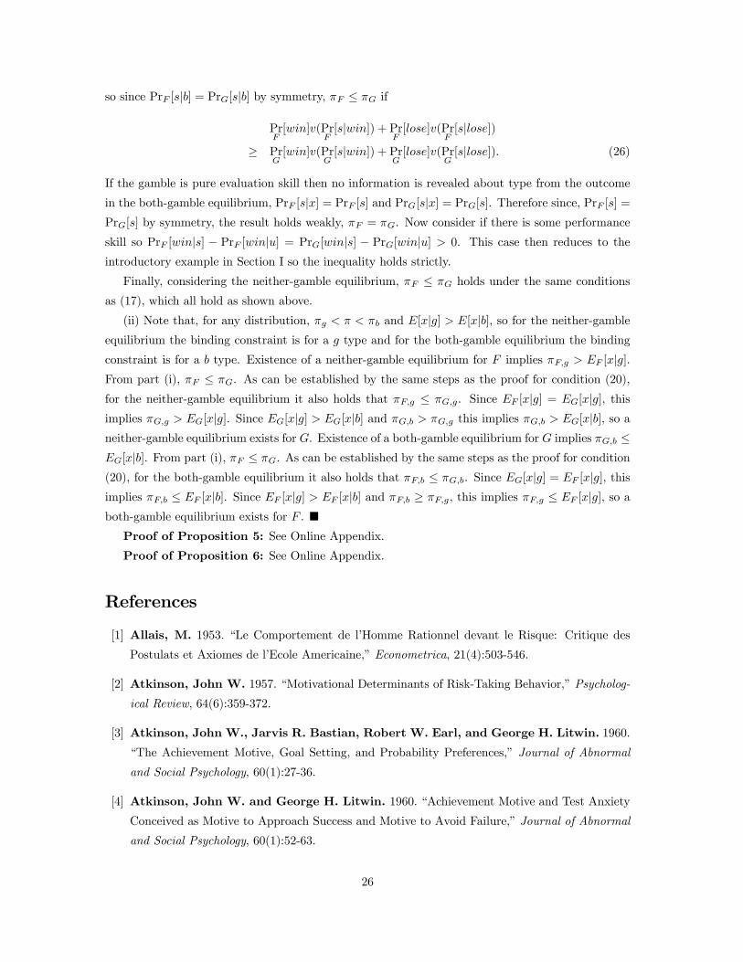
so since Pr [|] = Pr[|] by symmetry, ≤ if

Pr[](Pr

[|]) + Pr

[](Pr

[|])

≥ Pr[](Pr

[|]) + Pr

[](Pr

[|]) (26)

If the gamble is pure evaluation skill then no information is revealed about type from the outcome

in the both-gamble equilibrium, Pr [|] = Pr [] and Pr[|] = Pr[]. Therefore since, Pr [] =Pr[] by symmetry, the result holds weakly, = . Now consider if there is some performance

skill so Pr [|] − Pr [|] = Pr[|] − Pr[|] 0. This case then reduces to the

introductory example in Section I so the inequality holds strictly.

Finally, considering the neither-gamble equilibrium, ≤ holds under the same conditions

as (17), which all hold as shown above.

(ii) Note that, for any distribution, and [|] [|], so for the neither-gambleequilibrium the binding constraint is for a type and for the both-gamble equilibrium the binding

constraint is for a type. Existence of a neither-gamble equilibrium for implies [|].From part (i), ≤ . As can be established by the same steps as the proof for condition (20),

for the neither-gamble equilibrium it also holds that ≤ . Since [|] = [|], thisimplies [|]. Since [|] [|] and this implies [|], so aneither-gamble equilibrium exists for . Existence of a both-gamble equilibrium for implies ≤[|]. From part (i), ≤ . As can be established by the same steps as the proof for condition

(20), for the both-gamble equilibrium it also holds that ≤ . Since [|] = [|], thisimplies ≤ [|]. Since [|] [|] and ≥ , this implies ≤ [|], so aboth-gamble equilibrium exists for . ¥Proof of Proposition 5: See Online Appendix.

Proof of Proposition 6: See Online Appendix.

References

[1] Allais, M. 1953. “Le Comportement de l’Homme Rationnel devant le Risque: Critique des

Postulats et Axiomes de l’Ecole Americaine,” Econometrica, 21(4):503-546.

[2] Atkinson, John W. 1957. “Motivational Determinants of Risk-Taking Behavior,” Psycholog-

ical Review, 64(6):359-372.

[3] Atkinson, John W., Jarvis R. Bastian, Robert W. Earl, and George H. Litwin. 1960.

“The Achievement Motive, Goal Setting, and Probability Preferences,” Journal of Abnormal

and Social Psychology, 60(1):27-36.

[4] Atkinson, John W. and George H. Litwin. 1960. “Achievement Motive and Test Anxiety

Conceived as Motive to Approach Success and Motive to Avoid Failure,” Journal of Abnormal

and Social Psychology, 60(1):52-63.

26

[5] Avery, Christopher N. and Judith A. Chevalier. 1999. “Herding Over the Career,” Eco-

nomics Letters, 63(3):327-333.

[6] Banks, Jeffrey S. and Joel Sobel. 1987. “Equilibrium Selection in Signaling Games,” Econo-

metrica, 55(3):647-661.

[7] Barber, Brad M. and Terrance Odean. 2001. “Boys will be Boys: Gender, Overconfidence,

and Common Stock Investment,” Quarterly Journal of Economics, 116(1):261-292.

[8] Barberis, Nicholas and Richard Thaler. 2003. “A Survey of Behavioral Finance,” in Hand-

book of the Economics of Finance, edited by G.M. Constantinides, M. Harris and R. Stulz,

Elsevier Science.

[9] Bell, David E. 1982. “Regret in Decision Making under Uncertainty,” Operations Research,

30(5):961-981.

[10] Bell, David E. 1983. “Risk Premiums for Decision Regret,”Management Science, 29(10):1156-

1166.

[11] Benabou, Roland and Jean Tirole. 2002. “Self-Confidence and Personal Motivation,” Quar-

terly Journal of Economics, 117(3):871-915.

[12] Benabou, Roland and Jean Tirole. 2004. “Willpower and Personal Rules,” Journal of

Political Economy, 112(4):848-887.

[13] Bodner, Ronit and Drazen Prelec. 2003. “Self-Signaling and Diagnostic Utility in Everyday

Decision Making,” in I. Brocas and J. Carrillo eds., The Psychology of Economic Decisions. Vol.

1: Rationality and Well-Being. Oxford University Press.

[14] Bosch-Domenech, Antoni and Joaquim Silvestre. 2006. “Reflections on Gains and Losses:

a 2x2x7 Experiment,” Journal of Risk and Uncertainty, 33(3):217-235.

[15] Camerer, Colin. 2000. “Prospect Theory in the Wild: Evidence from the Field,” in Daniel

Khaneman and Amos Tversky eds., Choices, Values, and Frames, Cambridge University Press.

[16] Chevalier, Judith and Glenn Ellison. 1999. “Career Concerns of Mutual Fund Managers,”

Quarterly Journal of Economics, 114(2):389-432.

[17] Cho, In-Koo, and David M. Kreps. 1987. “Signaling Games and Stable Equilibria,” Quar-

terly Journal of Economics, 102(2):179-222.

[18] Coombs, Clyde H., Robyn M. Davies, and Amos Tversky. 1970. Mathematical Psy-

chology: An Elementary Introduction, Prentice-Hall, Englewood Cliffs, New Jersey.

[19] Cowen, Tyler and Amihai Glazer. 2007. “Esteem and ignorance,” Journal of Economic

Behavior and Organization, 63(3):373-383.

27

[20] Croson, Rachel and Uri Gneezy. 2009. “Gender Differences in Preferences,” Journal of

Economic Literature, 47(2):448-474.

[21] Dewatripont, Mathias, Ian Jewitt, and Jean Tirole. 1999. “The Economics of Career

Concerns, Part I: Comparing Information Structures,” Review of Economic Studies, 66(1):183-

198.

[22] Eckel, Catherine and Philip Grossman. “Men, Women, and Risk Aversion: Experimental

Evidence,” forthcoming, Handbook of Experimental Economic Results, 1: 1061-1073. Elsevier.

[23] Fishburn, Peter C. 1978. “On Handa’s ‘New Theory of Cardinal Utility’ and the Maximiza-

tion of Expected Return,” Journal of Political Economy, 86(2):321-324.

[24] Friedman, Milton and L.J. Savage.1948. “The Utility Analysis of Choices Involving Risk,”

Journal of Political Economy, 56(4):279-304.

[25] Gneezy, Uri, John A. List, and George Wu. 2006. “The Uncertainty Effect: When a Risky

Prospect is Valued Less Than its Worst Possible Outcome,” Quarterly Journal of Economics,

121(4):1283-1309.

[26] Gul, Faruk. 1991. “A Theory of Disappointment Aversion,” Econometrica, 59(3):667-686.

[27] Harbaugh, William T., Kate Krause, and Lise Vesterlund. 2002. “Risk Attitudes of

Children and Adults: Choices Over Small and Large Probability Gains and Losses,” Experi-

mental Economics, 5(1):53-84.

[28] Harbaugh, William T., Kate Krause, and Lise Vesterlund. “The Fourfold Pattern of

Risk Attitudes in Choice and Pricing Tasks,” forthcoming, Economic Journal.

[29] Holmstrom, Bengt. 1982. “Managerial Incentive Problems - A Dynamic Perspective,”

festschrift for Lars Wahlback (1982), republished in Review of Economic Studies, 66(1):169-

182.

[30] Holmstrom, Bengt and Joan Ricart I Costa. 1986. “Managerial Incentives and Capital

Management,” Quarterly Journal of Economics, 101(4):835-860.

[31] James, Henry. 1890. The Principles of Psychology, Henry Holt and Co., New York.

[32] Jianakoplos, Nancy Ammon and Alexandra Bernasek. 1998. “Are Women More Risk

Averse?”, Economic Inquiry, 36(4):620-1630.

[33] Jones, Edward E. and Steven Berglas. 1978. “Control of Attributions About the Self

Through Self-Handicapping Strategies: The Appeal of Alcohol and the Role of Underachieve-

ment,” Personality and Social Psychology Bulletin, 4(2):200-206.

[34] Kahneman, Daniel and Amos Tversky. 1979. “Prospect Theory: An Analysis of Decision

Under Risk,” Econometrica, 47(2):263-292.

28

[35] Kanodia, Chandra, Robert Bushman, and John Dickhaut. 1989. “Escalation Errors and

the Sunk Cost effect: An Explanation Based on Reputation and Information Asymmetries,”

Journal of Accounting Research, 27(1):59-77.

[36] Kimball, Miles S. 1990. “Precautionary Saving in the Small and in the Large,” Econometrica,

58(1):53-73.

[37] Kolditz, T.A. and R.M. Arkin. 1982. “An Impression Management Interpretation of the

Self-Handicapping Strategy,” Journal of Personality and Social Psychology, 43(3):492-502.

[38] Koszegi, Botond. 2006, “Ego Utility, Overconfidence, and Task Choice,” Journal of the Eu-

ropean Economic Association, 4(4):673-707.

[39] Laury, Susan K. and Charles A. Holt. 2008. “Further Reflections on the Reflection Effect,”

Research in Experimental Economics, 12, 404-440.

[40] Loomes, Graham and Robert Sugden.1982. “Regret Theory: An Alternative Theory of

Rational Choice Under Uncertainty,” Economic Journal, 92: 805-824.

[41] Menezes, C., C. Geiss, and J. Tressler. 1980. “Increasing Downside Risk,” American

Economic Review, 70(5):921-932.

[42] Milbourn, Todd T., Richard L. Shockley, and Anjan Thakor. 2001. “Managerial Career

Concerns and Investments in Information,” RAND Journal of Economics, 32(2):334-351.

[43] Morris, Stephen. 2001. “Political Correctness,” Journal of Political Economy, 109(2):231-265.

[44] Neilson, William S. 2006. “Victory and Defeat in Behavior Toward Risk,” working paper.

[45] Pratt, John W. 1964. “Risk Aversion in the Small and in the Large,” Econometrica,

32(1/2):122-136.

[46] Prelec, Drazen. 1998. “The Probability Weighting Function,” Econometrica, 66(3):497-528.

[47] Prendergast, Canice and Lars Stole. 1996 “Impetuous Youngsters and Jaded Old-Timers:

Acquiring a Reputation for Learning,” Journal of Political Economy, 104(6):1105-1134.

[48] Quiggin, John. 1982. “A Theory of Anticipated Utility,” Journal of Economic Behavior and

Organization, 3(4):323-343.

[49] Rabin, Matthew. 2000. “Risk Aversion and Expected Utility: A Calibration Theorem,”

Econometrica, 68(5):1281-1292.

[50] Rauh, Michael T. and Guilio Seccia. 2006. “Anxiety and Performance: An Endogenous

Learning-By-Doing Model,” International Economic Review, 47(2):583-610.

[51] Samuelson, Paul. 1963. “Risk and Uncertainty: A Fallacy of Large Numbers,” Scientia,

98:108-113.

29

[52] Scharfstein, David and Jeremy Stein. 1990. “Herd Behavior and Investment,” American

Economic Review, 80(3):465-479.

[53] Schelling, Thomas C. 1960. The Strategy of Conflict, Harvard University Press.

[54] Schlaifer, Robert. 1969. Analysis of Decisions Under Uncertainty, McGraw-Hill.

[55] Shefrin, Hersh and Meir Statman. 1985. “The Disposition to Sell Winners Too Early and

Ride Losers Too Long: Theory and Evidence,” Journal of Finance, 40(3):777-790.

[56] Thaler, Richard and Eric Johnson. 1990. “Gambling with the House Money and Trying to

Break Even: The Effects of Prior Outcomes in Risky Choice,” Management Science, 36(6):643-

660.

[57] Thaler, Richard and William T. Ziemba. 1988. “Parimutuel Betting Markets: Racetracks

and Lotteries,” Journal of Economic Perspectives, 2(2):161-174.

[58] Tversky, Amos and Daniel Kahneman. 1981. “The Framing of Decisions and the Psychol-

ogy of Choice,” Science, 211(4481):453-458.

[59] Tversky, Amos and Daniel Kahneman. 1992. “Advances in Prospect Theory: Cumulative

Representation of Uncertainty,” Journal of Risk and Uncertainty, 5(4):297-323.

[60] Whitmore, G. A. 1970. “Third-Degree Stochastic Dominance,” American Economic Review,

60(3):457-459

[61] Wu, George and Richard Gonzalez. 1996. “Curvature of the Probability Weighting Func-

tion,” Management Science, 42(12):1676-1690.

[62] Zwiebel, Jeffrey. 1995. “Corporate Conservatism,” Journal of Political Economy, 103(1):1-25.

30

6 Online Appendix

Proof of Proposition 5: Since the outcome is observed even if the gamble is not taken, in the sepa-

rating equilibrium the risk premium for type is = Pr[|](Pr[| ])+Pr[|](Pr[| ])−(Pr[|](Pr[| ]) + Pr[|](Pr[| ])), so the risk premium = Pr[] + Pr[] is

negative if

Pr[](Pr[| ]) + Pr[](Pr[| ]) Pr[](Pr[| ]) + Pr[](Pr[| ]) (27)

First suppose Pr[] 12. Applying Lemma 1, let = Pr[| ], = Pr[| ], =

Pr[| ], and = Pr[| ], and = Pr[]. Then (27) holds if

Pr[| ] Pr[| ] Pr[| ] Pr[| ] (28)

Pr[| ]− Pr[| ] ≥ Pr[| ]− Pr[| ] and (29)

Pr[] Pr[| ] + Pr[] Pr[| ]≥ Pr[] Pr[| ] + Pr[] Pr[| ] (30)

Regarding condition (28), Pr[| ] Pr[| ] is equivalent toµPr[|] + Pr[| ]− Pr[| ]

Pr[|] Pr[|] Pr[|]¶

(31)

µPr[|] + Pr[| ]− Pr[| ]

Pr[|] Pr[|] Pr[|]¶

⇐⇒ Pr[| ]− Pr[| ]Pr[|]

Pr[| ]− Pr[| ]Pr[|]

⇐⇒ Pr[|] Pr[|] ⇐⇒ Pr[|] + Pr[|] 1⇐⇒ Pr[ ] + Pr[ ] 12 ⇐⇒ Pr[] 12

where we have used the pure evaluation skill restriction Pr[|] = Pr[], the symmetry restrictionsthat Pr[| ] − Pr[| ] = Pr[| ] − Pr[| ] and Pr[] = Pr[] = 12, and the

evaluation skill condition that Pr[| ] Pr[| ]. Similarly Pr[| ] Pr[| ] isequivalent to

Pr[| ]− Pr[| ]Pr[|]

Pr[| ]− Pr[| ]Pr[|] (32)

⇐⇒ Pr[|] Pr[|]

which as shown in (31) holds for Pr[] 12. Finally Pr[| ] Pr[| ] is equivalent to

−Pr[| ]− Pr[| ]Pr[|]

Pr[| ]− Pr[| ]Pr[|] (33)

31

which holds since the LHS is negative and the RHS is positive. Regarding condition (29), the pure

evaluation skill restriction Pr[|] = Pr[] implies that it is equivalent toPr[| ]− Pr[| ]Pr[|] Pr[|] ≥ Pr[| ]− Pr[| ]

Pr[|] Pr[|] (34)

⇐⇒ Pr[|] Pr[|] ≥ Pr[|] Pr[|]⇐⇒ Pr[|](1− Pr[|]) ≥ Pr[|](1− Pr[|])⇐⇒ Pr[|]− Pr[|] ≥ Pr[|]2 − Pr[|]2

⇐⇒ Pr[|]− Pr[|] ≥ (Pr[|]− Pr[|]) (Pr[|] + Pr[|])

where we have used the symmetry restriction Pr[| ]−Pr[| ] = Pr[| ]−Pr[| ]and where the final inequality holds since Pr[|] + Pr[|] 1 as shown above. Finally,

regarding condition (30), note that for Pr[] = Pr[] the pure evaluation skill restriction that

Pr[|] = Pr[|] implies Pr[ ] = Pr[ ], which is equivalent to

Pr[ ] Pr[| ] + Pr[ ] Pr[| ]) (35)

= Pr[ ] Pr[| ] + Pr[ ] Pr[| ]⇐⇒ Pr[|] Pr[| ] + Pr[|] Pr[| ])= Pr[|] Pr[| ] + Pr[|] Pr[| ]⇐⇒ (Pr[|]− Pr[] + Pr[]) Pr[| ]

+ (Pr[|]− Pr[] + Pr[]) Pr[| ]= (Pr[|]− Pr[] + Pr[]) Pr[| ]

+ (Pr[|]− Pr[] + Pr[]) Pr[| ]⇐⇒ (Pr[|]− Pr[]) Pr[| ] + (Pr[|]− Pr[]) Pr[| ]

− (Pr[|]− Pr[]) Pr[| ]− (Pr[|]− Pr[]) Pr[| ]= Pr[] Pr[| ] + Pr[] Pr[| ]

−Pr[] Pr[| ]− Pr[] Pr[| ]

Therefore (30) holds if

(Pr[|]− Pr[]) Pr[| ] + (Pr[|]− Pr[]) Pr[| ] (36)

≥ (Pr[|]− Pr[]) Pr[| ] + (Pr[|]− Pr[]) Pr[| ]⇐⇒ (Pr[]− Pr[|]) (Pr[| ]− Pr[| ])≥ (Pr[|]− Pr[]) (Pr[| ]− Pr[| ])⇐⇒ Pr[| ]− Pr[| ] ≥ Pr[| ]− Pr[| ]

where we have used the implication from Pr[] = Pr[] that Pr[]−Pr[|] = Pr[|]−Pr[].The final inequality is the same condition as (29), so 0 for Pr[] 12. By the same arguments

0 for Pr[] 12.

32

Now consider the both-gamble equilibrium. By the same arguments as in the proof of Proposition

1, the D1 refinement requires that the observer believe an unexpected deviation to not gambling is

by type = . Therefore the risk premium is negative if

Pr[|](Pr[|]) + Pr[|](Pr[|]) (37)

Pr[|](Pr[| ]) + Pr[|](Pr[| ])

Since Pr[|] = Pr[|] = Pr[] in the both-gamble equilibrium of a pure evaluation skill gamble,this is equivalent to

(Pr[]) Pr[|](Pr[| ]) + Pr[|](Pr[| ]) (38)

For = this holds for 00 0 since Pr[|] Pr[| ] + Pr[|] Pr[| ] = Pr[ |] +Pr[ |] = Pr[|] = Pr[]. Using this result, for 00 0 this also holds for = if

Pr[|](Pr[| ]) + Pr[|](Pr[| ]) (39)

Pr[|](Pr[| ]) + Pr[|](Pr[| ])⇐⇒ (Pr[|]− Pr[|]) (Pr[| ]) (Pr[|]− Pr[|]) (Pr[| ])⇐⇒ (Pr[| ]) (Pr[| ])

where we have used the fact that Pr[|] Pr[|]. For 0 0 this last inequality holds if

Pr[| ] Pr[| ] (40)

⇐⇒ Pr[] +Pr[| ]− Pr[| ]

Pr[|] Pr[] Pr[]

Pr[]− Pr[| ]− Pr[| ]Pr[|] Pr[] Pr[]

⇐⇒ Pr[| ]− Pr[| ]Pr[|] −Pr[| ]− Pr[| ]

Pr[|]which holds by the pure evaluation skill assumption Pr[| ] Pr[| ].Now consider the neither-gamble equilibrium. The D1 refinement requires that the observer

believe an unexpected deviation to gambling is by type = so the risk premium is positive if

Pr[|](Pr[|]) + Pr[|](Pr[|]) (41)

Pr[|](Pr[| ]) + Pr[|](Pr[| ])

By similar logic as the both-gamble case, for 00 0 this holds for type = , and for 00 0 and

0 0 it holds for type = if

Pr[| ] Pr[| ] (42)

⇐⇒ Pr[] +Pr[| ]− Pr[| ]

Pr[|] Pr[] Pr[]

Pr[]− Pr[| ]− Pr[| ]Pr[|] Pr[] Pr[]

⇐⇒ Pr[| ]− Pr[| ]Pr[|] −Pr[| ]− Pr[| ]

Pr[|]

33

which holds by the evaluation skill assumption Pr[| ] Pr[| ]. ¥Proof of Proposition 6: Consider a single gamble and let = ( | = ) and =

( | = ). Then applying our results on risk premia for different types facing a single gamble, in

the separating equilibrium, the risk premium is higher for the gamble than the gamble if, from

(5) and (6),

(Pr[|])−[(Pr[| ])|] (Pr[|])−[(Pr[| ])|] (43)

⇐⇒ [(Pr[| ])|] [(Pr[| ])|]⇐⇒ Pr[|](Pr[| ]) + Pr[|](Pr[| ]) Pr[|](Pr[| ]) + Pr[|](Pr[| ])⇐⇒ (Pr[|]− Pr[|]) (Pr[| ]) (Pr[|]− Pr[|]) (Pr[| ])⇐⇒ (Pr[|]− Pr[|]) (Pr[| ]) (Pr[|]− Pr[|]) (Pr[| ])⇐⇒ (Pr[|]− Pr[|]) ((Pr[| ])− (Pr[| ])) 0

where the final inequality holds for 0 0 since Pr[|] Pr[|] and Pr[| ] Pr[| ].In the both-gamble equilibrium, the risk premium is weakly higher for the gamble than the

gamble if, from (9),

(Pr[|])−[(Pr[|])|] ≥ (Pr[|])−[(Pr[|])|] (44)

⇐⇒ [(Pr[|])|] ≤ [(Pr[|])|]⇐⇒ Pr[|](Pr[|]) + Pr[|](Pr[|])≤ Pr[|](Pr[|]) + Pr[|](Pr[|])⇐⇒ (Pr[|]− Pr[|]) ((Pr[|])− (Pr[|])) ≤ 0

where the final inequality holds for 0 0 since Pr[|] Pr[|] and Pr[|] ≥ Pr[|].In the neither-gamble equilibrium, the risk premium is higher for the gamble than the

gamble if, from (10),

(Pr[])−[(Pr[| ])|] (Pr[])−[(Pr[| ])|] (45)

which holds by the same arguments as for the separating equilibrium. ¥

34