Download pdf - Planck-scale effects on global symmetries: Cosmology of pseudo-Goldstone bosons

PHYSICAL REVIEW D 70, 115009 (2004)

Planck-scale effects on global symmetries: Cosmology of pseudo-Goldstone bosons

Eduard Masso, Francesc Rota, and Gabriel ZsembinszkiGrup de Fısica Teorica and Institut de Fısica d’Altes Energies, Universitat Autonoma de Barcelona

08193 Bellaterra, Barcelona, Spain(Received 30 April 2004; published 14 December 2004)

1550-7998=20

We consider a model with a small explicit breaking of a global symmetry, as suggested by gravitationalarguments. Our model has one scalar field transforming under a nonanomalous U�1� symmetry, andcoupled to matter and to gauge bosons. The spontaneous breaking of the explicitly broken symmetry givesrise to a massive pseudo-Goldstone boson. We analyze thermal and nonthermal production of this particlein the early universe, and perform a systematic study of astrophysical and cosmological constraints on itsproperties. We find that for very suppressed explicit breaking the pseudo-Goldstone boson is a cold darkmatter candidate.

DOI: 10.1103/PhysRevD.70.115009 PACS numbers: 14.80.Mz, 11.30.Qc, 95.35.+d

I. INTRODUCTION

It is generally believed that there is new physics beyondthe standard model of particle physics. At higher energies,new structures should become observable. Among them,there will probably be new global symmetries that are notmanifest at low energies. It is usually assumed that sym-metries would be restored at the high temperatures anddensities of the early universe.

However, the restoration of global symmetries might benot completely exact, since Planck-scale physics is be-lieved to break them explicitly. This feature comes fromthe fact that black holes do not have defined global chargesand, consequently, in a scattering process with black holes,global charges of the symmetry would not be conserved[1]. Wormholes provide explicit mechanisms of such non-conservation [2].

In the present article, we are concerned with the casethat the high temperature phase is only approximatelysymmetric. The breaking will be explicit, albeit small. Inthe process of spontaneous symmetry breaking (SSB),pseudo-Goldstone bosons (PGBs) with a small mass ap-pear. We explore the cosmological consequences of suchparticle species, in a simple model that exhibits the mainphysical features we would like to study.

The model has a (complex) scalar field ��x� transform-ing under a global, nonanomalous, U�1� symmetry. We donot need to specify which quantum number generates thesymmetry; it might be B-L, or a family U�1� symmetry,etc., We assume that the potential energy for � has asymmetric term and a symmetry-breaking term

V � Vsym � Vnon�sym: (1)

The symmetric part of the potential is

Vsym � 14��j�j2 � v2�2; (2)

where � is a coupling and v is the energy scale of the SSB.This part of the potential, as well as the kinetic termj@��j2, are invariant under the U�1� global transformation�! ei��.

04=70(11)=115009(12)$22.50 115009

Without any clue about the precise mechanism thatgenerates Vnon�sym, we work in an effective theory frame-work, where operators of order higher than four breakexplicitly the global symmetry. The operators would begenerated at the Planck scale MP � 1:2 1019 GeV andare to be used at energies below MP. They are multipliedby inverse powers of MP, so that when MP ! 1 the neweffects vanish.

The U�1� global symmetry is preserved by�?� � j�j2

but is violated by a single factor �. So, the simplest newoperator will contain a factor �

Vnon�sym � �g1

Mn�3P

j�jn��e�i� ��?ei��; (3)

with an integer n � 4. The coupling in (3) is in principlecomplex, so that we write it as ge�i� with g real. We willconsider that Vnon�sym is small enough so that it may beconsidered as a perturbation of Vsym. Even if (3) is alreadysuppressed by powers of the small factor v=MP, we willassume g small. In fact, after our phenomenological studywe will see that g must be tiny.

To study the modifications that the small explicitsymmetry-breaking term induces in the SSB process, weuse

� � �� v�ei�=v; (4)

with new real fields ��x� and the PGB ��x�. Introducing (4)in (3) we get

Vnon�sym � �2gv4�

vMP

�n�3cos

��v� �

�� : (5)

The dots refer to terms where ��x� is present. We see from(5) that there is a unique vacuum state, with h�i � �v. Tosimplify, we redefine �0 � �� v, and drop the prime, sothat the minimum is now at h�i � 0. From (5) we easilyobtain the � particle mass

m2� � 2g�

vMP

�n�1

M2P: (6)

-1 2004 The American Physical Society

9 10 11 12 13 14 15

-3 5

-3 0

-2 5

-2 0

-1 5

-1 0

-5

log(v/GeV)

log(

g)

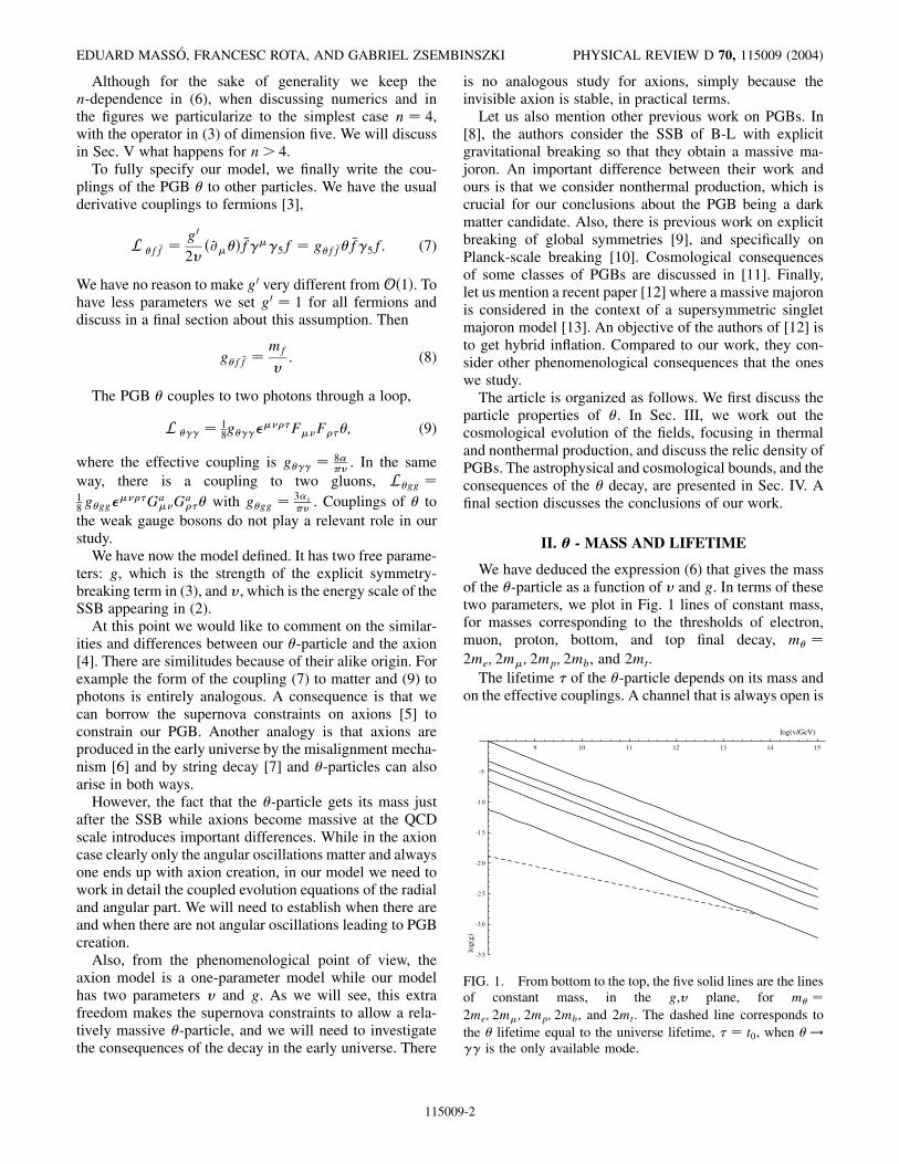
FIG. 1. From bottom to the top, the five solid lines are the linesof constant mass, in the g,v plane, for m� �

2me; 2m�; 2mp; 2mb, and 2mt. The dashed line corresponds tothe � lifetime equal to the universe lifetime, � � t0, when � !�� is the only available mode.

EDUARD MASSO, FRANCESC ROTA, AND GABRIEL ZSEMBINSZKI PHYSICAL REVIEW D 70, 115009 (2004)

Although for the sake of generality we keep then-dependence in (6), when discussing numerics and inthe figures we particularize to the simplest case n � 4,with the operator in (3) of dimension five. We will discussin Sec. V what happens for n > 4.

To fully specify our model, we finally write the cou-plings of the PGB � to other particles. We have the usualderivative couplings to fermions [3],

L �f �f �g0

2v�@�� f��5f � g�f �f� �f�5f: (7)

We have no reason to make g0 very different from O�1�. Tohave less parameters we set g0 � 1 for all fermions anddiscuss in a final section about this assumption. Then

g�f �f �mf

v: (8)

The PGB � couples to two photons through a loop,

L �� 18g��F��F��; (9)

where the effective coupling is g�� 8��v . In the same

way, there is a coupling to two gluons, L�gg �18 g�gg�

��Ga��G

a�� with g�gg � 3�s

�v . Couplings of � tothe weak gauge bosons do not play a relevant role in ourstudy.

We have now the model defined. It has two free parame-ters: g, which is the strength of the explicit symmetry-breaking term in (3), and v, which is the energy scale of theSSB appearing in (2).

At this point we would like to comment on the similar-ities and differences between our �-particle and the axion[4]. There are similitudes because of their alike origin. Forexample the form of the coupling (7) to matter and (9) tophotons is entirely analogous. A consequence is that wecan borrow the supernova constraints on axions [5] toconstrain our PGB. Another analogy is that axions areproduced in the early universe by the misalignment mecha-nism [6] and by string decay [7] and �-particles can alsoarise in both ways.

However, the fact that the �-particle gets its mass justafter the SSB while axions become massive at the QCDscale introduces important differences. While in the axioncase clearly only the angular oscillations matter and alwaysone ends up with axion creation, in our model we need towork in detail the coupled evolution equations of the radialand angular part. We will need to establish when there areand when there are not angular oscillations leading to PGBcreation.

Also, from the phenomenological point of view, theaxion model is a one-parameter model while our modelhas two parameters v and g. As we will see, this extrafreedom makes the supernova constraints to allow a rela-tively massive �-particle, and we will need to investigatethe consequences of the decay in the early universe. There

115009

is no analogous study for axions, simply because theinvisible axion is stable, in practical terms.

Let us also mention other previous work on PGBs. In[8], the authors consider the SSB of B-L with explicitgravitational breaking so that they obtain a massive ma-joron. An important difference between their work andours is that we consider nonthermal production, which iscrucial for our conclusions about the PGB being a darkmatter candidate. Also, there is previous work on explicitbreaking of global symmetries [9], and specifically onPlanck-scale breaking [10]. Cosmological consequencesof some classes of PGBs are discussed in [11]. Finally,let us mention a recent paper [12] where a massive majoronis considered in the context of a supersymmetric singletmajoron model [13]. An objective of the authors of [12] isto get hybrid inflation. Compared to our work, they con-sider other phenomenological consequences that the oneswe study.

The article is organized as follows. We first discuss theparticle properties of �. In Sec. III, we work out thecosmological evolution of the fields, focusing in thermaland nonthermal production, and discuss the relic density ofPGBs. The astrophysical and cosmological bounds, and theconsequences of the � decay, are presented in Sec. IV. Afinal section discusses the conclusions of our work.

II. � - MASS AND LIFETIME

We have deduced the expression (6) that gives the massof the �-particle as a function of v and g. In terms of thesetwo parameters, we plot in Fig. 1 lines of constant mass,for masses corresponding to the thresholds of electron,muon, proton, bottom, and top final decay, m� �

2me; 2m�; 2mp; 2mb, and 2mt.The lifetime � of the �-particle depends on its mass and

on the effective couplings. A channel that is always open is

-2

PLANCK-SCALE EFFECTS ON GLOBAL SYMMETRIES . . . PHYSICAL REVIEW D 70, 115009 (2004)

� ! ��. The corresponding width is

�� ! �� B��

�� g2��

m3�64�

; (10)

where B�� is the branching ratio. When m� > 2mf, thedecay � ! f �f is allowed and has a width

�� ! f �f� �Bf �f

�� g2

�f �f

m�

8�%; (11)

where % ��1� 4�

mf

m��2

q.

For masses m� < 2me the only available decay is intophotons. When we move to higher � masses, as soon asm� > 2me, we have the decay � ! e�e�. Actually, thenthe � ! e�e� channel dominates the decay because � !�� goes through one loop. However, �� ! �� / m3�whereas �� ! f �f� / m�. By increasing m� we reachthe value m� ’ 150me, where �� ! �� ’ �� !e�e��. For higher m� the channel � ! �� dominatesagain. If we continue increasing the � mass and cross thethreshold 2m�, the decay � ! �� dominates over � !

e�e� and � ! ��, because g�f �f is proportional to thefermion mass mf. This would be true until m� ’ 150m�,but before, the channel � ! p �p opens, and so on. Forlarger masses, each time a threshold 2mf opens up, � !

f �f happens to be the dominant decay mode.Now we can identify in Fig. 2 the regions with different

lifetimes. We start with the stability region � > t0 ’ 41017 s [14], the universe lifetime, a crucial region for thedark matter issue. When m� < 2me, � � t0 along thedashed line in Fig. 1 until v ’ 4 1013 GeV and alongthe line m� � 2me for higher v. Below these lines, relic �particles would have survived until now; in practical terms,for values of g and v in that region, we consider � as astable particle. Above the lines, � < t0 and the particle is

9 10 11 12 13 14 15

-3 5

-3 0

-2 5

-2 0

-1 5

-1 0

-5

6

7 5 3

2

4

6

5

4 3

4

5

1

3

stable

log(v/GeV)

log(

g)

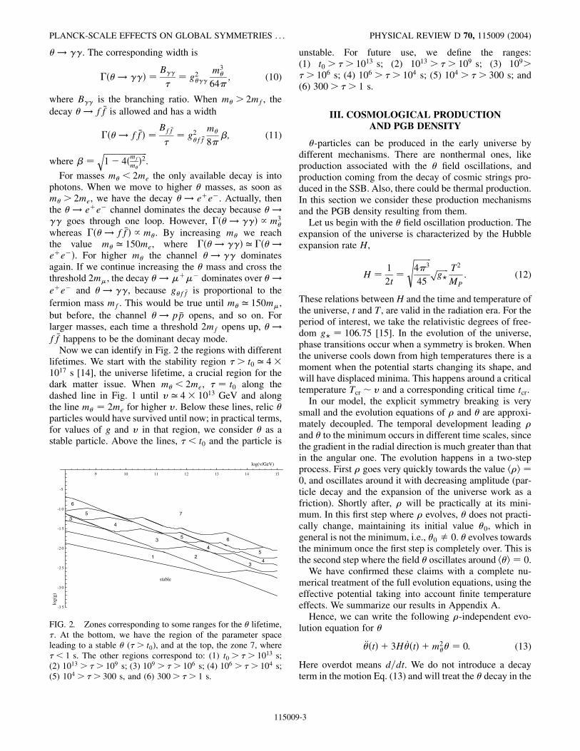
FIG. 2. Zones corresponding to some ranges for the � lifetime,�. At the bottom, we have the region of the parameter spaceleading to a stable � (� > t0), and at the top, the zone 7, where� < 1 s. The other regions correspond to: (1) t0 > � > 1013 s;(2) 1013 > � > 109 s; (3) 109 > � > 106 s; (4) 106 > � > 104 s;(5) 104 > � > 300 s, and (6) 300> � > 1 s.

115009

unstable. For future use, we define the ranges:(1) t0 > � > 1013 s; (2) 1013 > � > 109 s; (3) 109>� > 106 s; (4) 106 > � > 104 s; (5) 104 > � > 300 s; and(6) 300> � > 1 s.

III. COSMOLOGICAL PRODUCTIONAND PGB DENSITY

�-particles can be produced in the early universe bydifferent mechanisms. There are nonthermal ones, likeproduction associated with the � field oscillations, andproduction coming from the decay of cosmic strings pro-duced in the SSB. Also, there could be thermal production.In this section we consider these production mechanismsand the PGB density resulting from them.

Let us begin with the � field oscillation production. Theexpansion of the universe is characterized by the Hubbleexpansion rate H,

H �1

2t�

��4�3

45

s ��g?

p T2

MP: (12)

These relations between H and the time and temperature ofthe universe, t and T, are valid in the radiation era. For theperiod of interest, we take the relativistic degrees of free-dom g? � 106:75 [15]. In the evolution of the universe,phase transitions occur when a symmetry is broken. Whenthe universe cools down from high temperatures there is amoment when the potential starts changing its shape, andwill have displaced minima. This happens around a criticaltemperature Tcr � v and a corresponding critical time tcr.

In our model, the explicit symmetry breaking is verysmall and the evolution equations of � and � are approxi-mately decoupled. The temporal development leading �and � to the minimum occurs in different time scales, sincethe gradient in the radial direction is much greater than thatin the angular one. The evolution happens in a two-stepprocess. First � goes very quickly towards the value h�i �0, and oscillates around it with decreasing amplitude (par-ticle decay and the expansion of the universe work as afriction). Shortly after, � will be practically at its mini-mum. In this first step where � evolves, � does not practi-cally change, maintaining its initial value �0, which ingeneral is not the minimum, i.e., �0 � 0. � evolves towardsthe minimum once the first step is completely over. This isthe second step where the field � oscillates around h�i � 0.

We have confirmed these claims with a complete nu-merical treatment of the full evolution equations, using theeffective potential taking into account finite temperatureeffects. We summarize our results in Appendix A.

Hence, we can write the following �-independent evo-lution equation for �

��t� � 3H _��t� �m2�� 0: (13)

Here overdot means d=dt. We do not introduce a decayterm in the motion Eq. (13) and will treat the � decay in the

-3

9 10 11 12 13 14 15

-3 5

-3 0

-2 5

-2 0

-1 5

-1 0

-5

I

II

III

IV

log(

g)

log(v/GeV)

IV

V

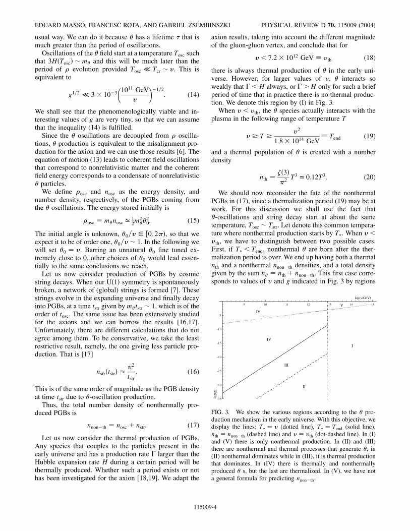
FIG. 3. We show the various regions according to the � pro-duction mechanism in the early universe. With this objective, wedisplay the lines: T� � v (dotted line), T� � Tend (solid line),nth � nnon�th (dashed line) and v � vth (dot-dashed line). In (I)and (V) there is only nonthermal production. In (II) and (III)there are nonthermal and thermal processes that generate �, in(II) nonthermal dominates while in (III), it is thermal productionthat dominates. In (IV) there is thermally and nonthermallyproduced � s, but the last are thermalized. In (V), we have nota general formula for predicting nnon�th.


usual way. We can do it because � has a lifetime � that ismuch greater than the period of oscillations.

Oscillations of the � field start at a temperature Tosc suchthat 3H�Tosc� �m� and this will be much later than theperiod of � evolution provided Tosc � Tcr � v. This isequivalent to

g1=2 � 3 10�3�1011 GeV

v

��1=2

: (14)

We shall see that the phenomenologically viable and in-teresting values of g are very tiny, so that we can assumethat the inequality (14) is fulfilled.

Since the � oscillations are decoupled from � oscilla-tions, � production is equivalent to the misalignment pro-duction for the axion and we can use those results [6]. Theequation of motion (13) leads to coherent field oscillationsthat correspond to nonrelativistic matter and the coherentfield energy corresponds to a condensate of nonrelativistic� particles.

We define �osc and nosc as the energy density, andnumber density, respectively, of the PGBs coming fromthe � oscillations. The energy stored initially is

�osc � m�nosc ’12m2��20: (15)

The initial angle is unknown, �0=v 2 �0; 2��, so that weexpect it to be of order one, �0=v� 1. In the following wewill set �0 � v. Barring an unnatural �0 fine tuned ex-tremely close to 0, other choices of �0 would lead essen-tially to the same conclusions we reach.

Let us now consider production of PGBs by cosmicstring decays. When our U�1� symmetry is spontaneouslybroken, a network of (global) strings is formed [7]. Thesestrings evolve in the expanding universe and finally decayinto PGBs, at a time tstr given by m�tstr � 1, which is of theorder of tosc. The same issue has been extensively studiedfor the axions and we can borrow the results [16,17].Unfortunately, there are different calculations that do notagree among them. To be conservative, we take the leastrestrictive result, namely, the one giving less particle pro-duction. That is [17]

nstr�tstr� �v2

tstr: (16)

This is of the same order of magnitude as the PGB densityat time tstr due to �-oscillation production.

Thus, the total number density of nonthermally pro-duced PGBs is

nnon�th � nosc � nstr: (17)

Let us now consider the thermal production of PGBs.Any species that couples to the particles present in theearly universe and has a production rate � larger than theHubble expansion rate H during a certain period will bethermally produced. Whether such a period exists or nothas been investigated for the axion [18,19]. We adapt the

115009

axion results, taking into account the different magnitudeof the gluon-gluon vertex, and conclude that for

v < 7:2 1012 GeV � vth (18)

there is always thermal production of � in the early uni-verse. However, for larger values of v, � interacts soweakly that �< H always, or �> H only for such a briefperiod of time that in practice there is no thermal produc-tion. We denote this region by (I) in Fig. 3.

When v < vth, the � species actually interacts with theplasma in the following range of temperature T

v � T �v2

1:8 1014 GeV� Tend (19)

and a thermal population of � is created with a numberdensity

nth �*�3�

�2T3 ’ 0:12T3; (20)

We should now reconsider the fate of the nonthermalPGBs in (17), since a thermalization period (19) may be atwork. For this discussion we shall use the fact that�-oscillations and string decay start at about the sametemperature, Tosc � Tstr. Let denote this common tempera-ture where nonthermal production starts by T�. When v <vth, we have to distinguish between two possible cases.First, if T� < Tend, nonthermal � are born after the ther-malization period is over. We end up having both a thermalnth and a nonthermal nnon�th densities, and a total densitygiven by the sum n� � nth � nnon�th. This first case corre-sponds to values of v and g indicated in Fig. 3 by regions

-4

9 10 11 12 13 14 15

-35

-30

-25

-20

-15

-10

-5

UNSTABLE

EXCLUDED DARKMATTER

log(v/GeV)

log(

g)

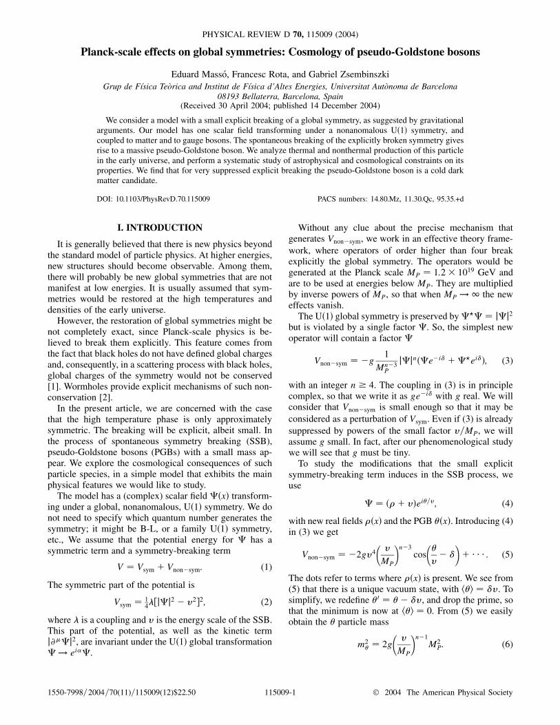
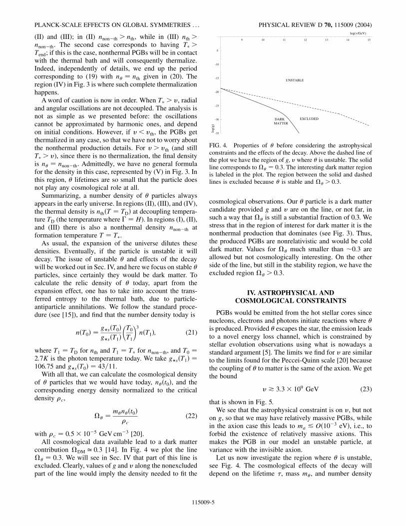
FIG. 4. Properties of � before considering the astrophysicalconstraints and the effects of the decay. Above the dashed line ofthe plot we have the region of g; v where � is unstable. The solidline corresponds to � � 0:3. The interesting dark matter regionis labeled in the plot. The region between the solid and dashedlines is excluded because � is stable and � > 0:3.


(II) and (III); in (II) nnon�th > nth, while in (III) nth >nnon�th. The second case corresponds to having T� >Tend; if this is the case, nonthermal PGBs will be in contactwith the thermal bath and will consequently thermalize.Indeed, independently of details, we end up the periodcorresponding to (19) with n� � nth given in (20). Theregion (IV) in Fig. 3 is where such complete thermalizationhappens.

A word of caution is now in order. When T� > v, radialand angular oscillations are not decoupled. The analysis isnot as simple as we presented before: the oscillationscannot be approximated by harmonic ones, and dependon initial conditions. However, if v < vth, the PGBs getthermalized in any case, so that we have not to worry aboutthe nonthermal production details. For v > vth (and stillT� > v), since there is no thermalization, the final densityis n� � nnon�th. Admittedly, we have no general formulafor the density in this case, represented by (V) in Fig. 3. Inthis region, � lifetimes are so small that the particle doesnot play any cosmological role at all.

Summarizing, a number density of � particles alwaysappears in the early universe. In regions (II), (III), and (IV),the thermal density is nth�T � TD� at decoupling tempera-ture TD (the temperature where � � H). In regions (I), (II),and (III) there is also a nonthermal density nnon�th atformation temperature T � T�.

As usual, the expansion of the universe dilutes thesedensities. Eventually, if the particle is unstable it willdecay. The issue of unstable � and effects of the decaywill be worked out in Sec. IV, and here we focus on stable �particles, since certainly they would be dark matter. Tocalculate the relic density of � today, apart from theexpansion effect, one has to take into account the trans-ferred entropy to the thermal bath, due to particle-antiparticle annihilations. We follow the standard proce-dure (see [15]), and find that the number density today is

n�T0� �g?s�T0�g?s�T1�

�T0T1

�3n�T1�; (21)

where T1 � TD for nth and T1 � T� for nnon�th, and T0 �2:7K is the photon temperature today. We take g?s�T1� �106:75 and g?s�T0� � 43=11.

With all that, we can calculate the cosmological densityof � particles that we would have today, n��t0�, and thecorresponding energy density normalized to the criticaldensity �c,

� �m�n��t0�

�c(22)

with �c � 0:5 10�5 GeV cm�3 [20].

All cosmological data available lead to a dark mattercontribution DM ’ 0:3 [14]. In Fig. 4 we plot the line � � 0:3. We will see in Sec. IV that part of this line isexcluded. Clearly, values of g and v along the nonexcludedpart of the line would imply the density needed to fit the

115009

cosmological observations. Our � particle is a dark mattercandidate provided g and v are on the line, or not far, insuch a way that � is still a substantial fraction of 0.3. Westress that in the region of interest for dark matter it is thenonthermal production that dominates (see Fig. 3). Thus,the produced PGBs are nonrelativistic and would be colddark matter. Values for � much smaller than �0:3 areallowed but not cosmologically interesting. On the otherside of the line, but still in the stability region, we have theexcluded region � > 0:3.

IV. ASTROPHYSICAL ANDCOSMOLOGICAL CONSTRAINTS

PGBs would be emitted from the hot stellar cores sincenucleons, electrons and photons initiate reactions where �is produced. Provided � escapes the star, the emission leadsto a novel energy loss channel, which is constrained bystellar evolution observations using what is nowadays astandard argument [5]. The limits we find for v are similarto the limits found for the Peccei-Quinn scale [20] becausethe coupling of � to matter is the same of the axion. We getthe bound

v * 3:3 109 GeV (23)

that is shown in Fig. 5.We see that the astrophysical constraint is on v, but not

on g, so that we may have relatively massive PGBs, whilein the axion case this leads to ma & O�10�3 eV�, i.e., toforbid the existence of relatively massive axions. Thismakes the PGB in our model an unstable particle, atvariance with the invisible axion.

Let us now investigate the region where � is unstable,see Fig. 4. The cosmological effects of the decay willdepend on the lifetime �, mass m�, and number density

-5

9 10 11 12 13 14 15

-3 5

-3 0

-2 5

-2 0

-1 5

-1 0

-5

SN1987A

log(v/GeV)lo

g(g)

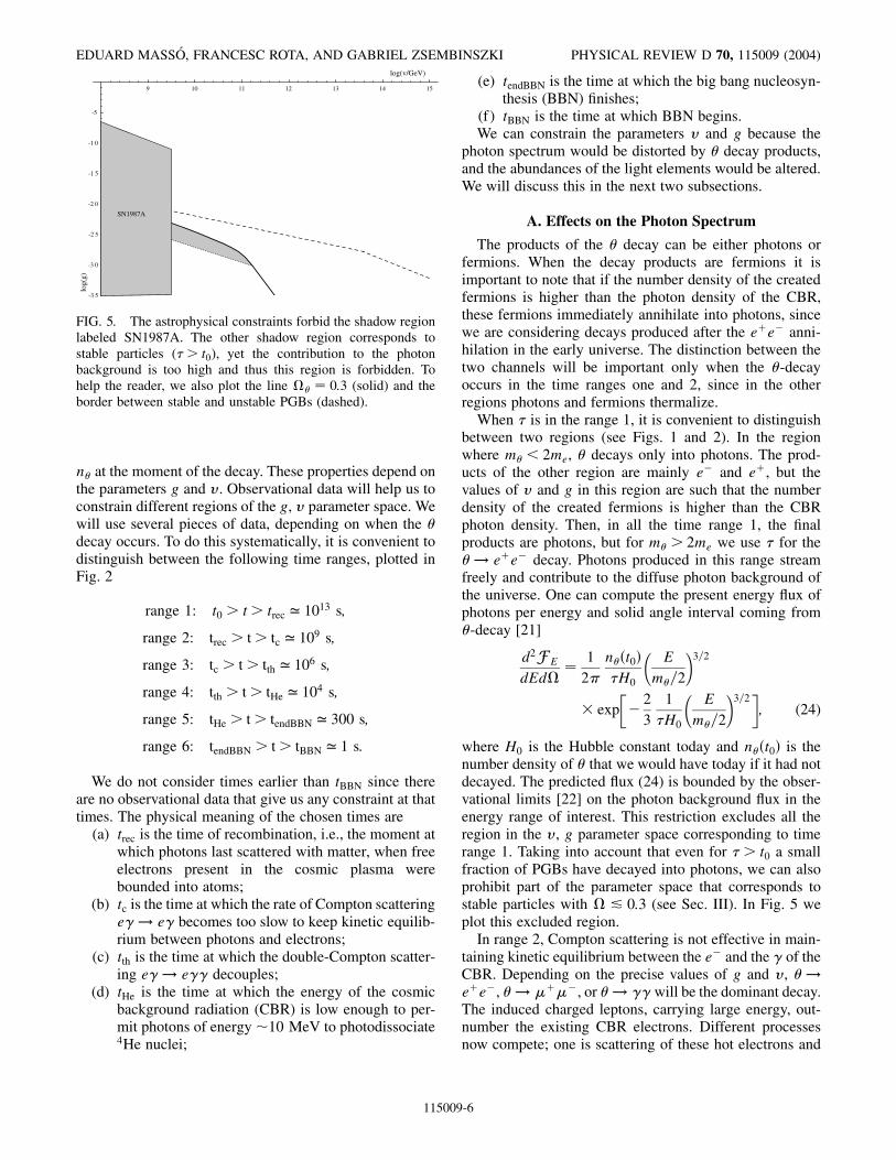
FIG. 5. The astrophysical constraints forbid the shadow regionlabeled SN1987A. The other shadow region corresponds tostable particles (� > t0), yet the contribution to the photonbackground is too high and thus this region is forbidden. Tohelp the reader, we also plot the line � � 0:3 (solid) and theborder between stable and unstable PGBs (dashed).


n� at the moment of the decay. These properties depend onthe parameters g and v. Observational data will help us toconstrain different regions of the g, v parameter space. Wewill use several pieces of data, depending on when the �decay occurs. To do this systematically, it is convenient todistinguish between the following time ranges, plotted inFig. 2

range 1: t0 > t > trec ’ 1013 s;

range 2: trec > t> tc ’ 109 s;

range 3: tc > t> tth ’ 106 s;

range 4: tth > t> tHe ’ 104 s;

range 5: tHe > t> tendBBN ’ 300 s;

range 6: tendBBN > t> tBBN ’ 1 s:

We do not consider times earlier than tBBN since thereare no observational data that give us any constraint at thattimes. The physical meaning of the chosen times are

(a) t
rec is the time of recombination, i.e., the moment atwhich photons last scattered with matter, when freeelectrons present in the cosmic plasma werebounded into atoms;
(b) t
c is the time at which the rate of Compton scatteringe� ! e� becomes too slow to keep kinetic equilib-rium between photons and electrons;
(c) t
th is the time at which the double-Compton scatter-ing e� ! e�� decouples;
(d) t
He is the time at which the energy of the cosmicbackground radiation (CBR) is low enough to per-mit photons of energy �10 MeV to photodissociate4He nuclei;
115009

(e) t

-6

endBBN is the time at which the big bang nucleosyn-thesis (BBN) finishes;

(f) t
BBN is the time at which BBN begins. We can constrain the parameters v and g because the
photon spectrum would be distorted by � decay products,and the abundances of the light elements would be altered.We will discuss this in the next two subsections.

A. Effects on the Photon Spectrum

The products of the � decay can be either photons orfermions. When the decay products are fermions it isimportant to note that if the number density of the createdfermions is higher than the photon density of the CBR,these fermions immediately annihilate into photons, sincewe are considering decays produced after the e�e� anni-hilation in the early universe. The distinction between thetwo channels will be important only when the �-decayoccurs in the time ranges one and 2, since in the otherregions photons and fermions thermalize.

When � is in the range 1, it is convenient to distinguishbetween two regions (see Figs. 1 and 2). In the regionwhere m� < 2me, � decays only into photons. The prod-ucts of the other region are mainly e� and e�, but thevalues of v and g in this region are such that the numberdensity of the created fermions is higher than the CBRphoton density. Then, in all the time range 1, the finalproducts are photons, but for m� > 2me we use � for the� ! e�e� decay. Photons produced in this range streamfreely and contribute to the diffuse photon background ofthe universe. One can compute the present energy flux ofphotons per energy and solid angle interval coming from�-decay [21]

d2F E

dEd �1

2�n��t0��H0

�E

m�=2

�3=2

exp��2

3

1

�H0

�E

m�=2

�3=2

�; (24)

where H0 is the Hubble constant today and n��t0� is thenumber density of � that we would have today if it had notdecayed. The predicted flux (24) is bounded by the obser-vational limits [22] on the photon background flux in theenergy range of interest. This restriction excludes all theregion in the v, g parameter space corresponding to timerange 1. Taking into account that even for � > t0 a smallfraction of PGBs have decayed into photons, we can alsoprohibit part of the parameter space that corresponds tostable particles with & 0:3 (see Sec. III). In Fig. 5 weplot this excluded region.

In range 2, Compton scattering is not effective in main-taining kinetic equilibrium between the e� and the � of theCBR. Depending on the precise values of g and v, � !e�e�, � ! ��, or � ! �� will be the dominant decay.The induced charged leptons, carrying large energy, out-number the existing CBR electrons. Different processesnow compete; one is scattering of these hot electrons and


muons with CBR photons. Another is e�e� and ��

annihilations that give high-energy photons, which heatCBR electrons. The last is high-energy photons producedin the decay � ! ��, that also scatter and heat CBRelectrons which in turn scatter with CBR photons.Whatever process is more important (it depends on the g,v values), the result is a distortion of the photon spectrum,parameterized by the Sunyaev-Zeldovich parameter y [23].The energy 'E dumped to the CBR, relative to the energyof the CBR itself is constrained by data on CBR spectrum[20]

'EECBR

’ 4y & 4:8 10�5 (25)

where 'E � m�n�. The experimental bound (26) rules outall the g and v values that would imply a lifetime � in thetime range 2.

In the range 3, Compton scattering is fast enough tothermalize the products of the �-decay occurring in thisrange. This is because even in the region where the prod-ucts are neither photons nor e�e�, the final particles willbe photons in any case. In this region the e� ! e��processes are not effective so the photon number cannotbe changed. So, after thermalization, one obtains a Bose-Einstein CBR spectrum with a chemical potential, f ��exp�E��=T � 1��1, instead of a black-body spectrum.The relation between � and 'E is [24]�

4

3

*�2�*�3�

�*�3�*�4�

��

'EECBR

�4

3

'n�

n�(26)

[*�n� is Riemann’s zeta function]. The parameter � is verywell constrained by CBR data [20] that gives j�j< 910�5. This value rules out all the g, v region that wouldgive � in the time range 3.

For times before the range 3, both Compton and double-Compton scattering are effective, so the decay productsthermalize with the CBR, without disturbing the black-body distribution but changing the evolution of the tem-perature of the thermal bath. This temperature variationleads to a change in the photon number, and thus to adecrease on the parameter 0 � nb=n�. The knowledgewe have on the value of this parameter at trec [14] andtendBBN [25] allows to constrain the g, v region that wouldgive lifetimes � in the time ranges four and 5. Although thecorresponding restriction is quite poor (it is essentially'E=ECBR & 1), yet it excludes the parameter space corre-sponding to the ranges four and 5. However, constraintsfrom the effects of the �-decay on the light element abun-dances are much more restrictive in these ranges, as we willexamine in the next subsection.

B. Effects on the Abundances of the Light Elements

The period of primordial nucleosynthesis is the earliestepoch where we have observational information. Also, thetheoretical predictions of the primordial yields of light

115009

elements are robust. The agreement with observation isconsidered one of the pillars of modern cosmology. The �decays, and the � particle itself, might modify the abun-dances of the light elements, which implies restrictions onthe v, g parameters.

First, we consider how the decays of a PGB affect theabundances of the light elements after they are synthesized,i.e., after tendBBN. One of the consequences of the decay isthe production of electromagnetic showers in the radiation-dominated plasma, initiated by the decay products. As aresult, photons of energy �10 MeV scatter and photodis-sociate light elements. This scattering occurs after tHe,because before tHe, the collision of these photons withthe CBR is more probable than with the light elements.In time range 4, the photodissociated element is deuterium(if m� > 10 MeV) [25] while in time ranges 3 and twothere is helium photodissociation (if m� > 100 MeV), withthe subsequent production of deuterium. Observationaldata for the abundance of deuterium constraint all theseprocesses. When � decays into quarks which hadronizesubsequently, hadronic showers can also be produced (ifm� � 1 GeV). These processes dissociate 4He before tHe,overproducing deuterium and lithium. All these con-straints, that are summarized in [25], exclude all the gand v values that give � in the time ranges 2, 3, 4, and 5,provided mass conditions are fulfilled for each case.However, values from ranges 2, 3, 4, and five that do notsatisfy the proper mass restrictions, are anyway excludedby the constraints we considered in the former subsection.

The other effect on the light element abundances arisesbecause the � particle would modify the BBN predictions.The presence of � and, more important, the presence of therelativistic products of the �-decay, accelerate the expan-sion rate of the universe in the relevant BBN period andmodify the synthesis of the light elements. The decay of the� boson is also a source of entropy production, which altersthe temperature evolution of the universe. This changes thenumber of photons (and the value of 0) and produces anearlier decoupling of neutrinos. Then the relation betweenT� and T� is changed, with potential effects on the BBNphysics. It is important to note that this production ofentropy never rises the temperature of the universe [26],and does not lead to several successive BBN periods. Allthese effects in BBN have been implemented [27] in theusual code, which allows to constrain the quantity 'E=n�.As a result, some of the values of g, v that would give � inthe time range six are ruled out. The potential effects ofhadronic showers, that we have mentioned earlier, alsowould modify the BBN results [25], allowing us to excludepart of the range 6, but not all of it.

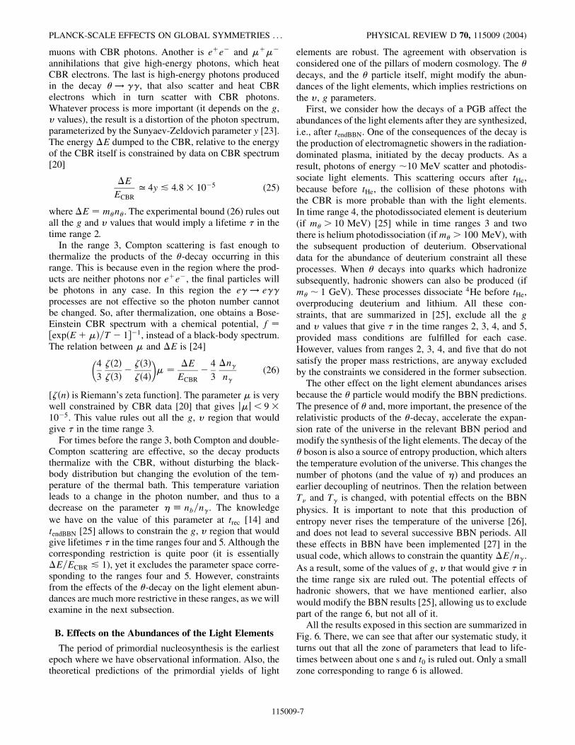
All the results exposed in this section are summarized inFig. 6. There, we can see that after our systematic study, itturns out that all the zone of parameters that lead to life-times between about one s and t0 is ruled out. Only a smallzone corresponding to range 6 is allowed.

-7

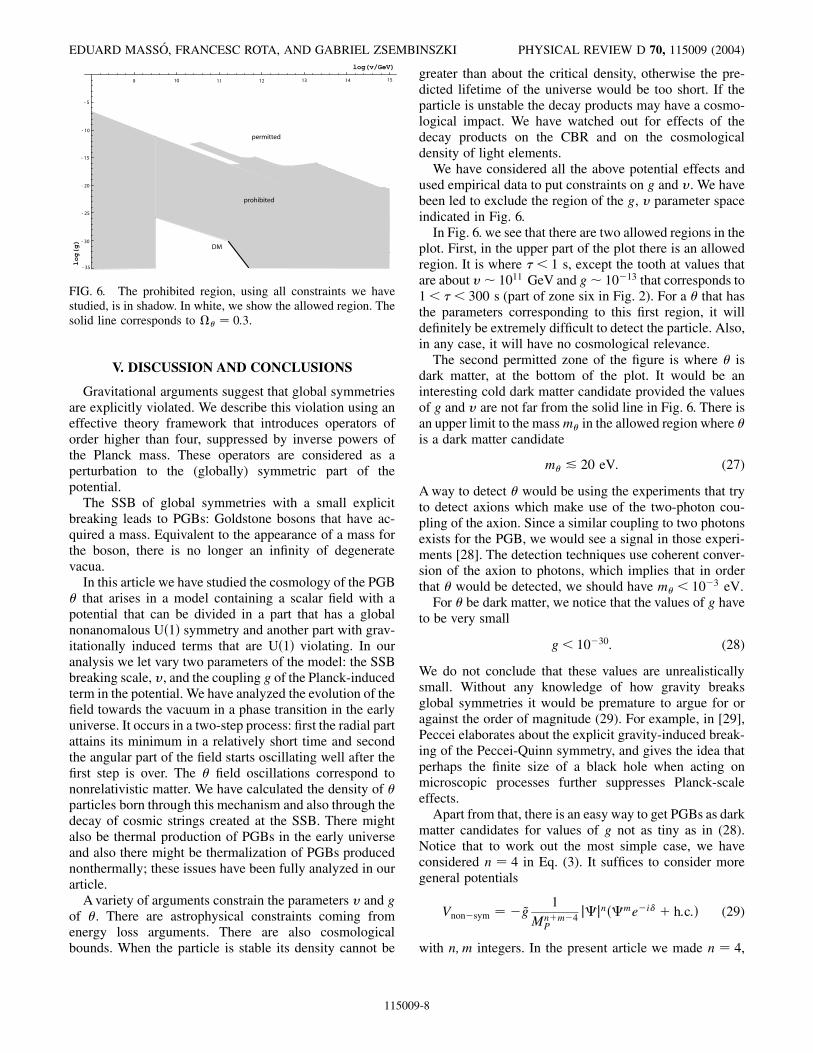
FIG. 6. The prohibited region, using all constraints we havestudied, is in shadow. In white, we show the allowed region. Thesolid line corresponds to � � 0:3.


V. DISCUSSION AND CONCLUSIONS

Gravitational arguments suggest that global symmetriesare explicitly violated. We describe this violation using aneffective theory framework that introduces operators oforder higher than four, suppressed by inverse powers ofthe Planck mass. These operators are considered as aperturbation to the (globally) symmetric part of thepotential.

The SSB of global symmetries with a small explicitbreaking leads to PGBs: Goldstone bosons that have ac-quired a mass. Equivalent to the appearance of a mass forthe boson, there is no longer an infinity of degeneratevacua.

In this article we have studied the cosmology of the PGB� that arises in a model containing a scalar field with apotential that can be divided in a part that has a globalnonanomalous U�1� symmetry and another part with grav-itationally induced terms that are U�1� violating. In ouranalysis we let vary two parameters of the model: the SSBbreaking scale, v, and the coupling g of the Planck-inducedterm in the potential. We have analyzed the evolution of thefield towards the vacuum in a phase transition in the earlyuniverse. It occurs in a two-step process: first the radial partattains its minimum in a relatively short time and secondthe angular part of the field starts oscillating well after thefirst step is over. The � field oscillations correspond tononrelativistic matter. We have calculated the density of �particles born through this mechanism and also through thedecay of cosmic strings created at the SSB. There mightalso be thermal production of PGBs in the early universeand also there might be thermalization of PGBs producednonthermally; these issues have been fully analyzed in ourarticle.

A variety of arguments constrain the parameters v and gof �. There are astrophysical constraints coming fromenergy loss arguments. There are also cosmologicalbounds. When the particle is stable its density cannot be

115009

greater than about the critical density, otherwise the pre-dicted lifetime of the universe would be too short. If theparticle is unstable the decay products may have a cosmo-logical impact. We have watched out for effects of thedecay products on the CBR and on the cosmologicaldensity of light elements.

We have considered all the above potential effects andused empirical data to put constraints on g and v. We havebeen led to exclude the region of the g, v parameter spaceindicated in Fig. 6.

In Fig. 6. we see that there are two allowed regions in theplot. First, in the upper part of the plot there is an allowedregion. It is where � < 1 s, except the tooth at values thatare about v� 1011 GeV and g� 10�13 that corresponds to1< � < 300 s (part of zone six in Fig. 2). For a � that hasthe parameters corresponding to this first region, it willdefinitely be extremely difficult to detect the particle. Also,in any case, it will have no cosmological relevance.

The second permitted zone of the figure is where � isdark matter, at the bottom of the plot. It would be aninteresting cold dark matter candidate provided the valuesof g and v are not far from the solid line in Fig. 6. There isan upper limit to the mass m� in the allowed region where �is a dark matter candidate

m� & 20 eV: (27)

A way to detect � would be using the experiments that tryto detect axions which make use of the two-photon cou-pling of the axion. Since a similar coupling to two photonsexists for the PGB, we would see a signal in those experi-ments [28]. The detection techniques use coherent conver-sion of the axion to photons, which implies that in orderthat � would be detected, we should have m� < 10�3 eV.

For � be dark matter, we notice that the values of g haveto be very small

g < 10�30: (28)

We do not conclude that these values are unrealisticallysmall. Without any knowledge of how gravity breaksglobal symmetries it would be premature to argue for oragainst the order of magnitude (29). For example, in [29],Peccei elaborates about the explicit gravity-induced break-ing of the Peccei-Quinn symmetry, and gives the idea thatperhaps the finite size of a black hole when acting onmicroscopic processes further suppresses Planck-scaleeffects.

Apart from that, there is an easy way to get PGBs as darkmatter candidates for values of g not as tiny as in (28).Notice that to work out the most simple case, we haveconsidered n � 4 in Eq. (3). It suffices to consider moregeneral potentials

Vnon�sym � �~g1

Mn�m�4P

j�jn��me�i� � h:c:� (29)

with n;m integers. In the present article we made n � 4,

-8


m � 1. If we take greater values, we get a suppression ofthe symmetry-breaking term due to extra factors v=MP andwe may allow values for ~g higher than the ones obtainedfor g. In order of magnitude, for v� 1011 GeV, we see thattaking operators of dimension n�m � 8 or 9 we have aPGB that is a dark matter candidate, but now with ~g�O�1�. In building the model we should have a reason forhaving the order of the operators starting at n�m > 5.The standard way is to impose additional discrete symme-tries in the theory.

Finally, we would like to comment on having put g0 � 1in (7). We could, of course, maintain g0 free, even we couldlet g0 be different for each fermion, but, in our opinion, theintroduction of extra parameters would make the physicalimplications of our model much less clear. This is why wefixed g0 � 1, but now it is time to think what happens forother values of g0.

The coupling g0 appears accompanying a factor propor-tional to the mass of the fermion and inversely proportionalto the energy breaking scale v, as expected for real andpseudo-Goldstone bosons. When a fermion has a U�1�charge, we have no reason to expect that g0 is much differ-ent than O�1�, but if a fermion has vanishing U�1� chargethen the coupling of � to this fermion may only go throughloops, and consequently we have a smaller g0. In this case,an important change concerns the astrophysical bound.Since g�NN is smaller than mN=v, the bound from super-nova is weakened and values of v smaller than 3:3109 GeV would be allowed. Another effect is that thebounds coming from the cosmological effects of the �decay are relaxed, since the lifetimes are longer when g0

is smaller. However, this does not mean that part of theprohibited region in Fig. 6 would be allowed. We have totake into account that nonthermal production is not alteredwhen changing g0 and therefore the bound � < 0:3 leadsto strong restrictions in the g; v parameter space. Also, �thermal production is suppressed with smaller g0.

9 10 11 12 13 14 15

-3 5

-3 0

-2 5

-2 0

-1 5

-1 0

-5

log(

g)

log(v/GeV)

permitted

prohibited

FIG. 7. Permitted and prohibited regions in the limit g0 ! 0.The solid line is � � 0:3 and the dotted line is T� � v. In theupper part of the dotted line we have no reliable way to calculate �.

115009

We would like to show graphically what would happenfor very small g0, and with this objective we show in Fig. 7the permitted and the prohibited regions in the limit g0 !0. At the view of the result, we conclude that one may havePGB as a dark matter candidate for much larger values of gthan obtained before in (29).

ACKNOWLEDGMENTS

We thank Mariano Quiros and Ramon Toldra for veryuseful discussions. We acknowledge support by the CICYTResearch Project No. FPA2002-00648, by the EU networkon Supersymmetry and the Early Universe (HPRN-CT-2000-00152), and by the Departament d’Universitats,Recerca i Societat de la Informacio (DURSI), ProjectNo. 2001SGR00188. One of us (G. Z.) is supported bythe DURSI, under Grant No. 2003FI 00138.

APPENDIX A

1. How to Obtain the Effective Potential Veff

We present here in some detail how to find the effectivepotential that gives us a complete description of the physicsinvolved in our model. Following the standard procedure[30], taking into account the finite temperature effects, weare led to a new contribution to Vsym, which is given by

V% �1

2�2%4JB�m2%2�

�1

2�2%4Z 1

0dxx2 ln�1� e�

��x2�%2m2

p�; (A1)

where JB is the thermal bosonic function and % � 1=T,and m2 � � 1

2�v2 � ��?�� 1

2�T2 is the effective mass.

With (A1), we see the behavior of the finite temperatureeffective potential. For practical applications, it is conve-nient to use a high temperature expansion of V% [31]written in the form

V% ’1

24m2T2 �

1

12�m3T �

1

64�2m4 ln

m2=T2

223:63; (A2)

where we have neglected terms independent of the field.The effective potential must contain the explicit symmetry-breaking term of our model, Vnon�sym. Using for � theparametrization � � 3ei�=v, the expression for this termis

Vnon�sym � �2g3n�1

Mn�3P

cos��v

�: (A3)

Thus, our effective potential will be written as the sum ofthree terms

Veff � Vsym � V% � Vnon�sym: (A4)

-9

0.02 0.04 0.06 0.08 0.1 0.12 0.14

1

η=Log (t/tc)

φ(η)

θ(η)~

~0.4

0.2

0.6

0.8

2 4 6 8 10 12

-0.2

1

η=Log (t/tcr)

θ(η)~

0.4

0.2

0.6

0.8

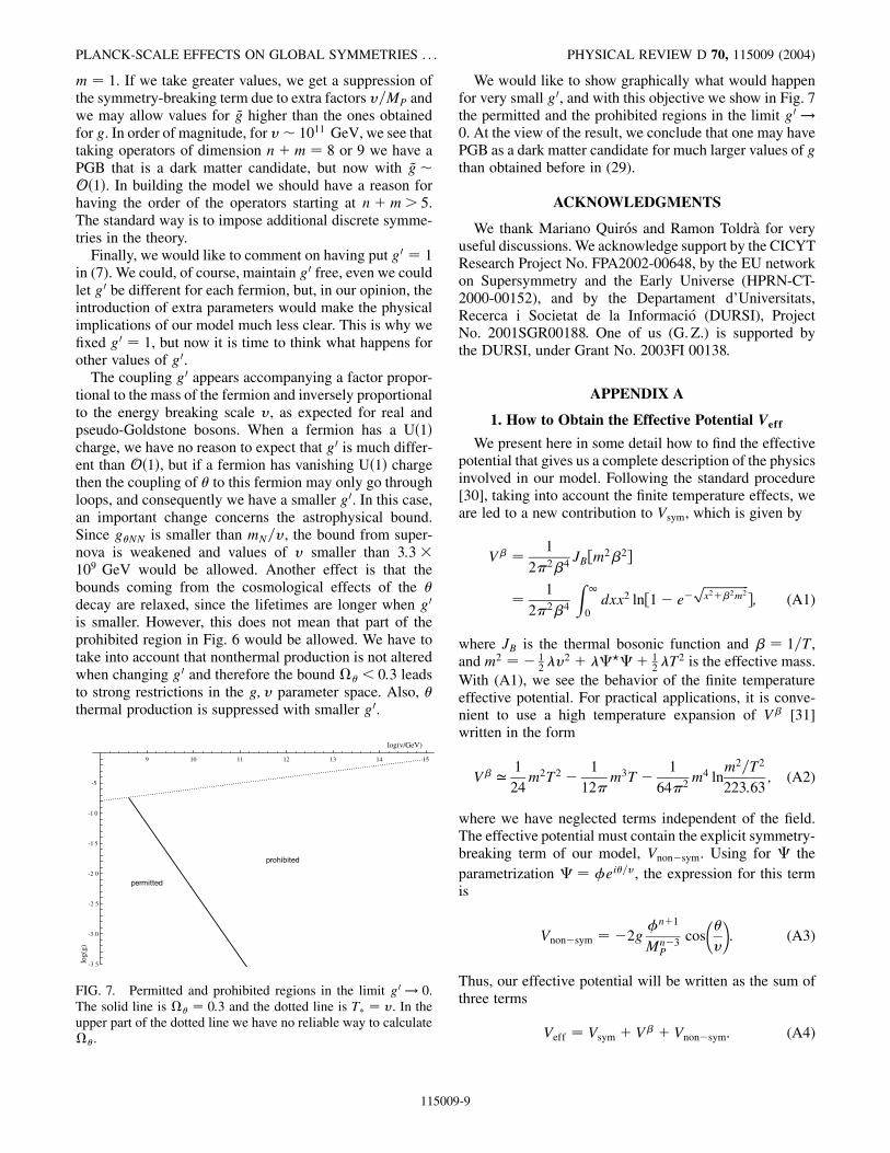
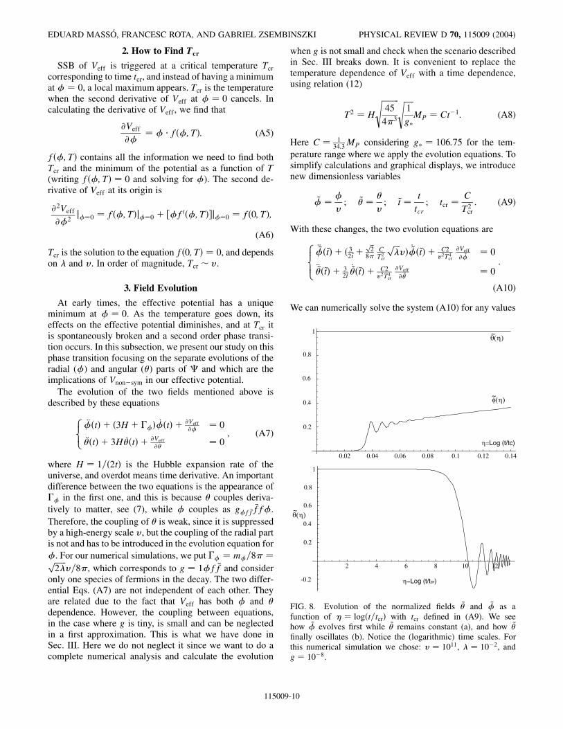
FIG. 8. Evolution of the normalized fields ~� and ~3 as afunction of 0 � log�t=tcr� with tcr defined in (A9). We seehow ~3 evolves first while ~� remains constant (a), and how ~�finally oscillates (b). Notice the (logarithmic) time scales. Forthis numerical simulation we chose: v � 1011, � � 10�2, andg � 10�8.


2. How to Find Tcr

SSB of Veff is triggered at a critical temperature Tcrcorresponding to time tcr, and instead of having a minimumat 3 � 0, a local maximum appears. Tcr is the temperaturewhen the second derivative of Veff at 3 � 0 cancels. Incalculating the derivative of Veff , we find that

@Veff@3

� 3 f�3; T�: (A5)

f�3; T� contains all the information we need to find bothTcr and the minimum of the potential as a function of T(writing f�3; T� � 0 and solving for 3). The second de-rivative of Veff at its origin is

@2Veff@32

j3�0 � f�3; T�j3�0 � �3f0�3; T��j3�0 � f�0; T�;

(A6)

Tcr is the solution to the equation f�0; T� � 0, and dependson � and v. In order of magnitude, Tcr � v.

3. Field Evolution

At early times, the effective potential has a uniqueminimum at 3 � 0. As the temperature goes down, itseffects on the effective potential diminishes, and at Tcr itis spontaneously broken and a second order phase transi-tion occurs. In this subsection, we present our study on thisphase transition focusing on the separate evolutions of theradial (3) and angular (�) parts of � and which are theimplications of Vnon�sym in our effective potential.

The evolution of the two fields mentioned above isdescribed by these equations8<:

�3�t� � �3H � �3� _3�t� � @Veff@3 � 0

��t� � 3H _��t� � @Veff@� � 0

; (A7)

where H � 1=�2t� is the Hubble expansion rate of theuniverse, and overdot means time derivative. An importantdifference between the two equations is the appearance of�3 in the first one, and this is because � couples deriva-tively to matter, see (7), while 3 couples as g3f �f

�ff3.Therefore, the coupling of � is weak, since it is suppressedby a high-energy scale v, but the coupling of the radial partis not and has to be introduced in the evolution equation for3. For our numerical simulations, we put �3 � m3=8� ��2�

pv=8�, which corresponds to g � 13f �f and consider

only one species of fermions in the decay. The two differ-ential Eqs. (A7) are not independent of each other. Theyare related due to the fact that Veff has both 3 and �dependence. However, the coupling between equations,in the case where g is tiny, is small and can be neglectedin a first approximation. This is what we have done inSec. III. Here we do not neglect it since we want to do acomplete numerical analysis and calculate the evolution

115009

when g is not small and check when the scenario describedin Sec. III breaks down. It is convenient to replace thetemperature dependence of Veff with a time dependence,using relation (12)

T2 � H

��45

4�3

s ��1

g�

sMP � Ct�1: (A8)

Here C � 134:3MP considering g� � 106:75 for the tem-

perature range where we apply the evolution equations. Tosimplify calculations and graphical displays, we introducenew dimensionless variables

~3 �3v; ~� �

�v; ~t �

ttcr; tcr �

C

T2cr: (A9)

With these changes, the two evolution equations are8><>:�~3�~t� � � 32~t �

��2

p

8�CT2cr

��

pv� _~3�~t� � C2

v2T4cr

@Veff@ ~3

� 0

�~��~t� � 32~t_~��~t� � C2

v2T4cr

@Veff@~�

� 0:

(A10)

We can numerically solve the system (A10) for any values

-10


of interest for v and g. In Fig. 8, we show one such solutionfor arbitrarily chosen values for v; g, and �, for n � 4.

4. Discussion

In Sec. III we based our work on the fact that, due to thesmallness of the explicit symmetry breaking, the fieldevolution towards its minimum occurs in a two-step pro-cess: firstly, the radial field goes quickly towards its vac-uum expectation value, oscillates around it for a finite timetill it stops due to the expansion of the universe andcoupling to fermions; secondly, the angular field staysconstant much longer and finally starts to oscillate aroundits minimum. We have proved numerically that this is so;we have checked it by solving the system Eqs. (A10) for avariety of values of our parameters.

We would like to specify the upper limit on g for ourmodel to make sense. The parameter g is considered to betoo large when the term Vnon�sym in the effective potentialstarts to dominate over the other ones, for 3� v. Whenthis happens, the explicit symmetry breaking is so big that,where the absolute minimum of the effective potential issupposed to be, the first derivative of Veff with respect to 3is negative and there is no minimum at all. In this case,there makes no sense talking about angular oscillationsaround the minimum. Therefore, by comparing the��=4�34 term with Vnon�sym, one obtains an upper limitfor g

g <�8

MP

v: (A11)

115009

We have numerically checked that, for parameter valuesof interest to us, radial oscillations start very early and theyare very rapidly damped, at a time scale much less than thetime when �-oscillations start. One example is plotted inFig. 8. What happens is that the radial field oscillates for asmall time around the minimum of the symmetric part ofthe effective potential and after the oscillations stop, thefield stays at the minimum and evolves in time untiltemperature effects are irrelevant and the minimum stabil-izes at ~3 � 1�3 � v�. Thus, for values of g that satisfy(A11) and (14), when angular oscillations start, the radialones have already stopped and we must not worry about thepossibility that the two oscillations happened at the sametime. More important is to impose the condition that whenradial oscillations start, the minimum of Veff be locatedclose to the value 3 � v in order to have initial conditionsfor �-oscillations also of order v. With all this in mind, forv values in the range of interest �108 < v < 1015 GeV�, weget to the conclusion that g must be smaller that about 10�5

(the number depends slightly on v and �). In particular,considering values of interest for � to be a dark mattercandidate (v� 1011 GeV) and �� 10�2, we obtain anapproximate limit g < 10�5. This upper limit is alsoroughly given by the dotted line represented in Fig. 3,which corresponds to T� � v. Obviously, values for g�10�30 and v� 1011 GeV which we have found to beinteresting to have � as a reasonable dark matter candidateof the universe, are consistent with our mechanism ofproducing � particles.

[1] See for instance T. Banks, Physicalia Magazine 12, 19(1990), and references therein.

[2] S. B. Giddings and A. Strominger, Nucl. Phys. B307, 854(1988); S. R. Coleman, Nucl. Phys. B310, 643 (1988); G.Gilbert, Nucl. Phys. B328, 159 (1989).

[3] G. B. Gelmini, S. Nussinov, and T. Yanagida, Nucl. Phys.B219, 31 (1983).

[4] S. Weinberg, Phys. Rev. Lett. 40, 223 (1978); F. Wilczek,Phys. Rev. Lett. 40, 279 (1978).

[5] For a comprehensive review, see G. G. Raffelt, Stars AsLaboratories For Fundamental Physics (University ofChicago Press, Chicago, 1996).

[6] J. Preskill, M. B. Wise, and F. Wilczek, Phys. Lett. B 120,127 (1983); L. F. Abbott and P. Sikivie, Phys. Lett. B 120,133 (1983); M. Dine and W. Fischler, Phys. Lett. B 120,137 (1983).

[7] A. Vilenkin and E. P. S. Shellard, Cosmic Strings and otherTopological Defects (Cambridge University Press,Cambridge, 1994); A. Vilenkin and A. E. Everett, Phys.Rev. Lett. 48, 1867 (1982).

[8] E. K. Akhmedov, Z. G. Berezhiani, R. N. Mohapatra, andG. Senjanovic, Phys. Lett. B 299, 90 (1993).

[9] C. T. Hill and G. G. Ross, Phys. Lett. B 203, 125 (1988);

C. T. Hill and G. G. Ross, Nucl. Phys. B311, 253 (1988).[10] M. Lusignoli, A. Masiero, and M. Roncadelli, Phys. Lett.

B 252, 247 (1990); S. Ghigna, M. Lusignoli, and M.Roncadelli, Phys. Lett. B 283, 278 (1992); D. Grasso,M. Lusignoli, and M. Roncadelli, Phys. Lett. B 288, 140(1992).

[11] C. T. Hill, D. N. Schramm, and J. N. Fry, Nucl. Part. Phys.19, 25 (1989); A. K. Gupta, C. T. Hill, R. Holman, andE. W. Kolb, Phys. Rev. D 45, 441 (1992); J. A. Frieman,C. T. Hill, and R. Watkins, Phys. Rev. D 46, 1226 (1992);J. A. Frieman, C. T. Hill, A. Stebbins, and I. Waga, Phys.Rev. Lett. 75, 2077 (1995).

[12] D. Kazanas, R. N. Mohapatra, S. Nasri, and V. L. Teplitz,Phys. Rev. D 70, 033015 (2004).

[13] R. N. Mohapatra and X. Zhang, Phys. Rev. D 49, 1163(1994); 49, 6246 (1994).R. N. Mohapatra and A. Riotto,Phys. Rev. Lett. 73, 1324 (1994).

[14] C. L. Bennett et al., Astrophys. J. Suppl. Ser. 148, 1(2003).

[15] E. W. Kolb and M. S. Turner, The Early Universe,Frontiers in Physics Vol. 69 (Addison-Wesley, RedwoodCity, US, 1990) p. 547.

[16] R. L. Davis, Phys. Lett. B 180, 225 (1986); R. A. Battye

-11


and E. P. S. Shellard, Phys. Rev. Lett. 73, 2954 (1994); 76,2203 (1996); R. L. Davis, Phys. Rev. D 32, 3172 (1985);R. A. Battye and E. P. S. Shellard, Nucl. Phys. B423, 260(1994); M. Yamaguchi, M. Kawasaki, and J. Yokoyama,Phys. Rev. Lett. 82, 4578 (1999).

[17] D. Harari and P. Sikivie, Phys. Lett. B 195, 361 (1987); C.Hagmann and P. Sikivie, Nucl. Phys. B363, 247 (1991); C.Hagmann, S. Chang, and P. Sikivie, Phys. Rev. D 63,125018 (2001).

[18] M. S. Turner, Phys. Rev. Lett. 59, 2489 (1987); 60, 1101E(1988).

[19] E. Masso, F. Rota, and G. Zsembinszki, Phys. Rev. D 66,023004 (2002).

[20] Particle Data Group Collaboration, K. Hagiwara et al.,Phys. Rev. D 66, 010001 (2002).

[21] E. Masso and R. Toldra, Phys. Rev. D 60, 083503 (1999).

115009

[22] M. T. Ressell and M. S. Turner, Bull. Am. Astron. Soc. 22,753 (1990).

[23] R. A. Sunyaev and Y. B. Zeldovich, Annu. Rev. Astron.Astrophys. 18, 537 (1980).

[24] E. Masso and R. Toldra, Phys. Rev. D 55, 7967 (1997).[25] S. Sarkar, Rep. Prog. Phys. 59, 1493 (1996).[26] R. J. Scherrer and M. S. Turner, Phys. Rev. D 31, 681

(1985).[27] R. J. Scherrer and M. S. Turner, Astrophys. J. 331, 19

(1988); Astrophys. J. 331, 33 (1988).[28] For a recent review, see E. Masso, Nucl. Phys. (Proc.

Suppl.) 114, 67 (2003).[29] R. D. Peccei, hep-ph/0009030.[30] See, for example, M. Quiros, hep-ph/9901312.[31] L. Dolan and R. Jackiw, Phys. Rev. D 9, 3320 (1974).

-12