Download pdf - Plan Lesson 3: Sampling - UNIL · 5 Quantitative approaches Sampling: quantitative and qualitative "First, the term "sampling" is problematic for qualitative research, because it

1

Quantitative approaches

Lesson 3:

Sampling

2


Plan

1. Introduction to quantitative sampling

2. Sampling error and sampling bias

3. Response rate

4. Types of "probability samples"

5. The size of the sample

6. Types of "non-probability samples"

3


1. Introduction to quantitative sampling

4


Sampling: Definition

Sampling = choosing the unities (e.g. individuals,

famililies, countries, texts, activities) to beinvestigated

5


Sampling: quantitative and qualitative"First, the term "sampling" is problematic for qualitative research,because it implies the purpose of "representing" the population sampled.

Quantitative methods texts typically recognize only two main types ofsampling: probability sampling (such as random sampling) andconvenience sampling."

(...) any nonprobability sampling strategy is seen as "conveniencesampling" and is strongly discouraged."

This view ignores the fact that, in qualitative research, the typical way ofselecting settings and individuals is neither probability sampling norconvenience sampling."

It falls into a third category, which I will call purposeful selection; otherterms are purposeful sampling and criterion-based selection."

This is a strategy in which particular settings, persons, or activieties areselected deliberately in order to provide information that can't be gottenas well from other choices."Maxwell , Joseph A. , Qualitative research design..., 2005 , 88

6


Population and Sample

Population

Sample

SamplingIIIIIIIIIIIIIIII

IIIIIIIIIIIIIIII

IIIIIIIIIIIIIIII

IIIIIIIIIIIIIIII

IIIIIIIIIIIIIIII

IIIII

IIIII

(= «!Miniature population!»)

7


Population, Sample, Sampling frame

Population = ensemble of unities from which the sample istaken

Sample = part of the population that is chosen for investigation. The choice may be based onrandomness or not.

Sampling

frame = list of all the unities from which the choice ismade.

8


Representative sample, probability sample

Representative sample = Sample that reflects the populationin a reliable way: the sample is a«!miniature population!»

Probability sample = Sample that has been randomlychosen. Therefore, every unity hasa known probability to be chosen.

9


Representativity: an empirical question

The representativity of the sample cannot be assured byfollowing a given method. If we use the correct methods(random choice, stratification etc.) we can only maximize theprobability of producing a representative sample.

It is an empirical question (and should be tested) if thesample is really representative of the population.

For example: we would investigate if the percentage ofwomen in the sample are not significantly different fromthose of the population (==> the sample is representativeconcerning gender).

10


2. Sampling error, sampling bias

11


Errors: different types

1. Sampling error due to chance, size of sample

2. Sampling bias not due to chance or size of sample. E.g. non-response linkedto the specific theme of the research

3. Data collection error e.g. bad question wording; bad interviewing

4. Data processing error e.g. wrong coding

5. Data analysis error e.g. wrong statistical model;erroneous data analysis

6. Data interpretation error e.g. wrong interpretation of results

12


Sampling error, sampling bias

Sampling error = Differences between the sample and thepopulation that are due to the sampling(the randomness). Sampling error can bediminished by increasing the size of thesample

Sampling bias = Differences between the sample and thepopulation that are not due to sampling(the randomness); the sampling biasdoes not diminish with increased samplesize.

13


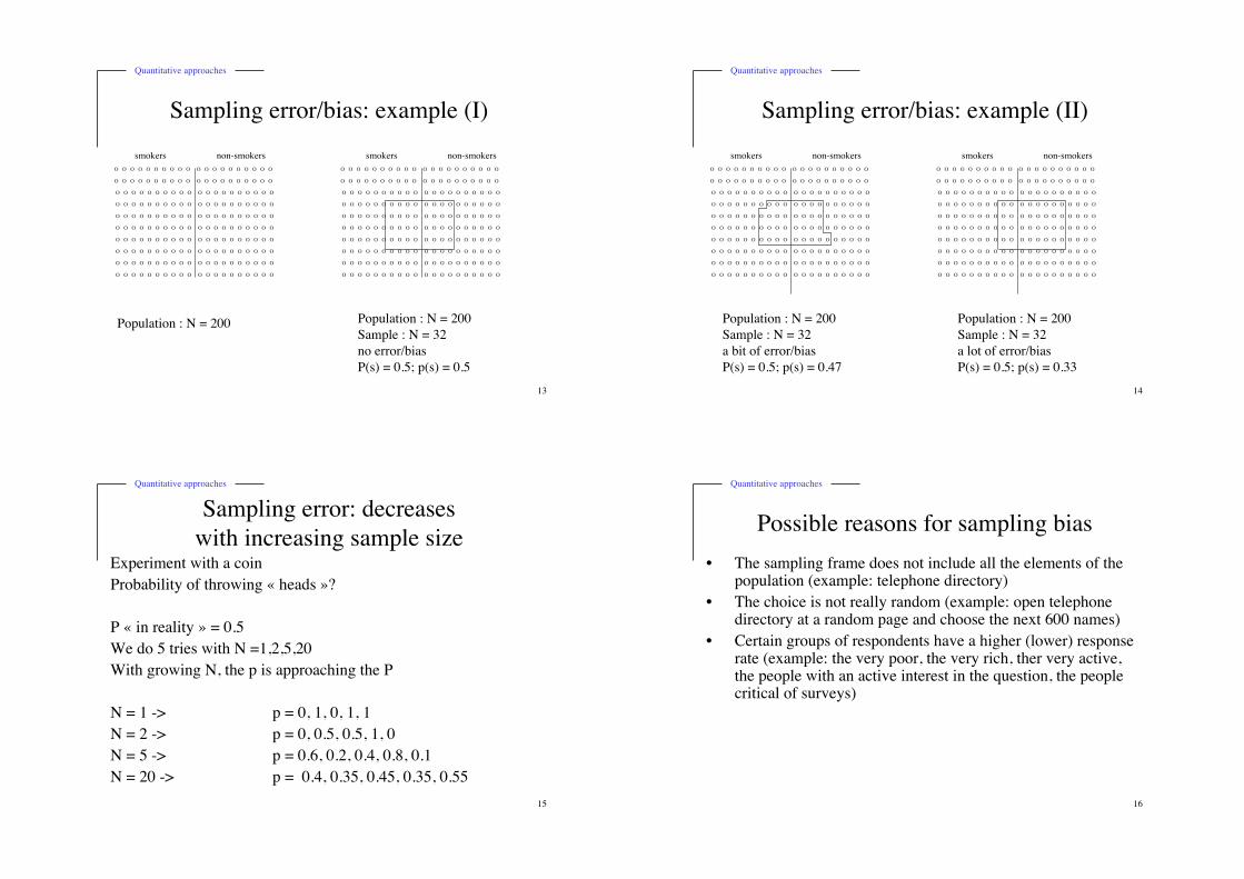
Sampling error/bias: example (I)

O O O O O O O O O O O O O O O O O O O O










smokers non-smokers

Population : N = 200











smokers non-smokers


Sample : N = 32

no error/bias

P(s) = 0.5; p(s) = 0.5

14


Sampling error/bias: example (II)











smokers non-smokers


Sample : N = 32

a bit of error/bias

P(s) = 0.5; p(s) = 0.47











smokers non-smokers


Sample : N = 32

a lot of error/bias

P(s) = 0.5; p(s) = 0.33

15


Sampling error: decreases

with increasing sample sizeExperiment with a coin

Probability of throwing «!heads!»?

P «!in reality!» = 0.5

We do 5 tries with N =1,2,5,20

With growing N, the p is approaching the P

N = 1 -> p = 0, 1, 0, 1, 1

N = 2 -> p = 0, 0.5, 0.5, 1, 0

N = 5 -> p = 0.6, 0.2, 0.4, 0.8, 0.1

N = 20 -> p = 0.4, 0.35, 0.45, 0.35, 0.55

16


Possible reasons for sampling bias

• The sampling frame does not include all the elements of thepopulation (example: telephone directory)

• The choice is not really random (example: open telephonedirectory at a random page and choose the next 600 names)

• Certain groups of respondents have a higher (lower) responserate (example: the very poor, the very rich, ther very active,the people with an active interest in the question, the peoplecritical of surveys)

17


Sampling error vs. sampling bias: Citation

Sampling error is random. Every time you select an individual, a text, asituation, or any "unit of observation," that unit of observation will bedifferent from the population of such units. Hence you always have anerror (we hope a small one) in generalizing to the population of units."

"Unlike sampling error, "sampling bias" is systematic (nonrandom). Forexample, if for a focus group study you "randomly" select one of everyfive students who happen to be in the library on a Friday afternonnon,you might have a biased sample that does not represent the views of"average" college students."

"Unlike sampling error, increasing the size of the samle does notdecrease the degree of bias in your sample."

Obviously, the results of a biased sample cannot be considered to berepresentative of the population (i.e. , the findings have lowtransferability or external validity)."Tashakkori / Teddlie, Mixed Methodology. Combining Qualitative and Quantitative ..., S.72-73

18


3. Response rate

19


Response rate

Response rate= Percentage of individuals of the samplewho have responded to the questionnaire

N of returned interviews - N returned interviews, not usable

Sample - number of individuals who were not able to

answer or could not be reached

=

=

652 - 8

1212 - 66= 0.56

Example

20


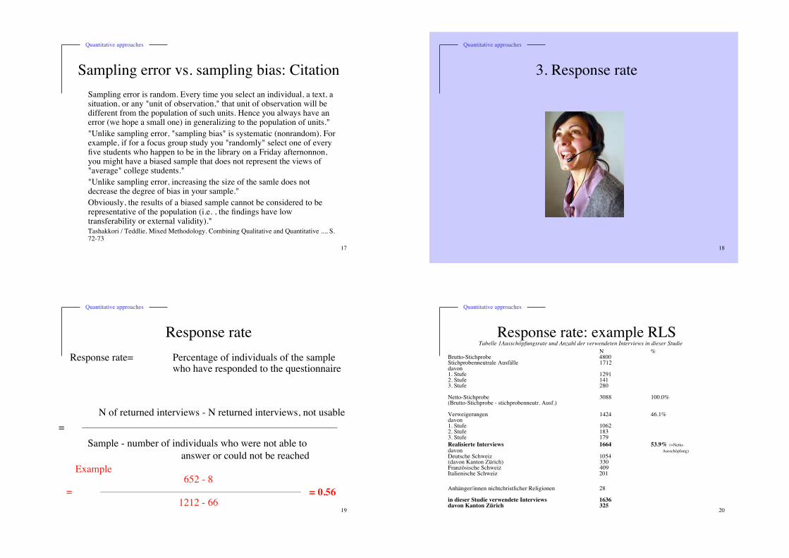
Response rate: example RLSTabelle 1Ausschöpfungsrate und Anzahl der verwendeten Interviews in dieser Studie

N %Brutto-Stichprobe 4800Stichprobenneutrale Ausfälle 1712davon1. Stufe 12912. Stufe 1413. Stufe 280

Netto-Stichprobe 3088 100.0%(Brutto-Stichprobe - stichprobenneutr. Ausf.)

Verweigerungen 1424 46.1%davon1. Stufe 10622. Stufe 1833. Stufe 179

Realisierte Interviews 1664 53.9% (=Netto-

davon Ausschöpfung)

Deutsche Schweiz 1054(davon Kanton Zürich) 330Französische Schweiz 409Italienische Schweiz 201

Anhänger/innen nichtchristlicher Religionen 28

in dieser Studie verwendete Interviews 1636davon Kanton Zürich 325

21


Response rate: example

Christliches Zeugnis• Der tatsächliche Rücklauf war besser als erwartet. Von 942

angeschriebenen Personen antworteten 469 auf das ersteSchreiben(49,8%); nach erfolgter Mahnung sandten weitere125 Personen (13,3%) gültige Fragebogen ein. DieGesamtrücklaufquote beläuft sich damit auf rund 63% (594Personen).

• Dies nach Abzug der ungültigen Antworten und derBefragten, die nicht mehr aufzufinden, krank oder gestorbenwaren.

22


4. Types of probability sample

23


Types of probability sample

4.1. Simple random sample

4.2. Systematic random sample

4.3. Stratified random sampling

4.4. Multi-stage cluster sampling

24


4.1 Simple random sample

Simple random sample = choose randomly a predetermined number of thepopulation (sample frame)

1. decide what population to use

2. choose the sampling frame

3. decide sample size

4. use random numbers (e.g. with the help of a computer) inorder to choose the units)

25


4.2 Systematic random sample

Systematic sample = choose randomly/systematically apredetermined number of thepopulation (sample frame)

1. decide what population to use

2. choose the sampling frame

3. decide sample size

4. begin with a random number between 1 and i; choose everyith unit in the sampling frame. i = sample / population

26


Systematic random sample:

Christliches Zeugnis (I)

Ziel war, eine für den Evangelikalismus der deutschen

Schweiz repräsentative Untersuchung durchzuführen.

Als Methode wurde die schriftliche Befragung gewählt. In

einem nächsten Schritt musste eine geeignete Adresskartei

aller Evangelikalen gefunden werden, um die repräsentative

Stichprobe ziehen zu können. Eine solche Kartei existiert

nicht - und es ist schwierig, ja fast unmöglich, eine sinnvolle

Stichprobe selbst zu konstruieren. (...)

Auf der Suche nach einem Ausweg aus dieser Schwierigkeit

stiessen wir auf Campus für Christus, eine evangelikal

ausgerichtete Organisation.

27



Christliches Zeugnis (II)

Sie gibt eine Zeitschrift, das "Christliche Zeugnis", heraus,

welche innerhalb des Evangelikalismus recht weit verbreitet

ist und eine Auflage von ca. 20000 erreicht. Von der Kartei

dieser Zeitschriftenempfänger kann man hoffen, dass sie ein

unverzerrtes Bild des E in der deutschen Schweiz liefert.

Die Zufallsstichprobe wurde wie folgt gezogen: Die erste

Adresse wurde durch eine Nummer zwischen 1 und 20

zufällig gewählt; dann wurden von hier aus in 20-er-

Schritten die weiteren Adressen aussortiert. Als gültig

erwiesen sich 942 Adressen.

28



Study on islamophobia

The data used for this study stem from a closed-question

face-to-face survey, each interview taking from 45-60

minutes. The population consisted of inhabitants of the city

of Zurich in the age range 18 to 65 with Swiss nationality.

The survey was conducted between October 1994 and March

1995 by the Sociological Institute of the University of

Zurich. The people were chosen randomly from the official

files of the state (Einwohnerkontrolle). In all, 1,138

interviews were conducted. The response rate was 72%. The

survey can be regarded as representative of the Swiss

population of the city of Zurich (Stolz, 2000, 226).

29


4.3 Stratified random sampling

Stratified random sampling: create strata in your samplingframe corresponding to centralcleavages in your popultion.Inside every strata, choosepredetermined numbers of unitsrandomly.

30


Stratified random sampling: example (1)

On sait que dans notre population de 7'000'000 nous avons72% de germanophones, 20% de francophones et 8%d'italophones. Notre sample size est 1000.

Alors nous décidons de chosir aléatoirement

dans la population des germanophones: 720

dans la population des francophones: 200

dans la population des italophones: 80

-> Concernant la langue, notre sample est absolumentreprésentatif.

-> Si nous avions effectué un simple random sample, lesampling erreur aurait produit p.ex. un sample avec: germ:742, franc: 195, ital: 63

31


Stratified random sampling: example (2)

In the NCS-CH study, we stratified for religious tradition.Furthermore, we overweighted smaller religious traditions.

32


4.4 Multi-stage cluster sampling

Multi-stage cluster sampling = on choisit d'abord aléatoirement des groupesd'unités (clusters); puis, onchoisit aléatoirement dans cesgroupes

-> Souvent moins cher

33


Multi-stage cluster sampling:

Etude sur les évangéliques (Milieu) (I)Some 1,850 questionnaires were given out and 1,100 werereturned, giving a response rate of 59.4%. The response ratewas 57.9% (N= 359) for the charismatic group, 54.6%(N=377) for the moderate and 66.9% (N= 361) for thefundamentalist group. Being a mail survey, these responserates can be seen as very satisfactory. The data was collectedbetween June 2003 and September 2003. This sample can besaid to be representative of the members of evangelical freechurches in Switzerland. For a number of analyses weaggregated the data sets from 1999 and 2003. One of thecentral features of the design of our study on evangelical freechurches was to include a large number of questions that hadalready been used in the 1999 survey of the Swisspopulation, in order to be able to compare the evangelicalmilieu to the „societal environment“.

34



Etude sur les évangéliques (Milieu)(II)

• Our data stem from two representative surveys, oneconducted in 1999 covering the whole population ofSwitzerland, and a second survey from 2003 among themembers of the evangelical free churches in Switzerland.The first data set (1999) was produced by conducting 1,562computer-aided telephone interviews (CATI), based on arandom sample of the inhabitants of Switzerland within theage-range of 16 to 75. Response rate was 54%.

35



Etude sur les évangéliques (Milieu) (III)

The second data set (2003) was produced by a mail survey of

1,100 evangelicals from evangelical free churches in

Switzerland, based on a stratified cluster sample. Cluster

sampling was effectuated by randomly choosing evangelical

free churches from a list and then randomly selecting

members from these churches. Stratification was achieved by

dividing the sample into three groups: charismatic, moderate

and fundamentalist. Since the fundamentalist group in our

population only amounts to about 11%, the fundamentalist

stratum was overrepresented in the sample, in order to be

able to make a better comparison between the three groups.36


5. The size of the sample

37


Size matters!

The larger the sample, the better you fare!

With larger samples,

- your estimates of the parameters gain in precision(confidence intervals are getting smaller)

- the differences you find will become significant easier

- you will be able to make analyses at a more detailed level(comparing various subgroups etc.)

38


Size : absolute and relative

It is not the relative but the absolute size that matters.

-> A random sample of 1000 has the same «!value!» if thepopulation is Switzerland or China

39


Formula

Arithmetic mean = x =

xi

i=1

n

!

n

Standard deviation = s =

(xi! x)

2

i=1

n

"

n !1Variance = s

2=

(xi! x)

2

i=1

n

"

n !1

Standard error = sx=

s

n

95% confidence interval = X ± z0.25sx

(z0.25 = 1.96)40


Example : increasing the sample size

decreases the confidence intervalWhat is the true mean in the population?

Mean in the sample (n = 105): 4.8

standard deviation (sample) = 1.2

standard error (mean) = 1.2/ 105 = 0.117

confidence interval: true mean = 4.8 +- 1.96 * 0.117

-> between 4.571 et 5.029

Mean in the sample (n = 1000): 4.8

standard deviation (sample) = 1.2

standard error (mean) = 1.2/ 1000 = 0.00694

confidence interval: true mean = 4.8 +- 1.96 * 0.00694

-> entre 4.7864 et 4.8136

41


Factors influencing the size of the sample

Coûts: from n = 1000 on for the sample, the gains in precision aredecreasing

Non-response: a certain percentage of individuals will refuse to participate;we therefore have to start out with a larger sample

Heterogeneity: If the heterogeneity of the the sample is large, we have tohave a larger sample.

Type of analysis: If we want to analyze the relationship between manyvariables at the same time (multivariate analysis), we haveto have a larger sample (e.g. sex * age * political

preference)

42


The example of the dwarfs

43


Sampling error: decreases

with growing NIn this example, we imagine an infinite population of dwarfs. We wouldlike to know their mean hight and the variance of their hight in thepopulation.

The question: how many dwarfs do we have to draw randomly from thepopulation in order to measure them and then estimate the populationhight and variance?

In the following simulation we draw 30 samples for different N’s (for N=5,10,15,20....100).

The «!real!» mean in the population is 10 cm. The «!real!» variance in thepopulation is 4 (standard deviation = 2)

The simulation shows that for samples smaller than N = 40, the estimateof the mean and variance are very unreliable. 44


Simulation with R

Simulation with R

plot(c(0,100),c(0,15),type="n",xlab="Samplesize",ylab="Variance", cex.lab=1.2)

for (df in seq(5,100,5)){

for(i in 1:30){

x<-rnorm(df,mean=10,sd=2)

points(df,var(x))}}

45


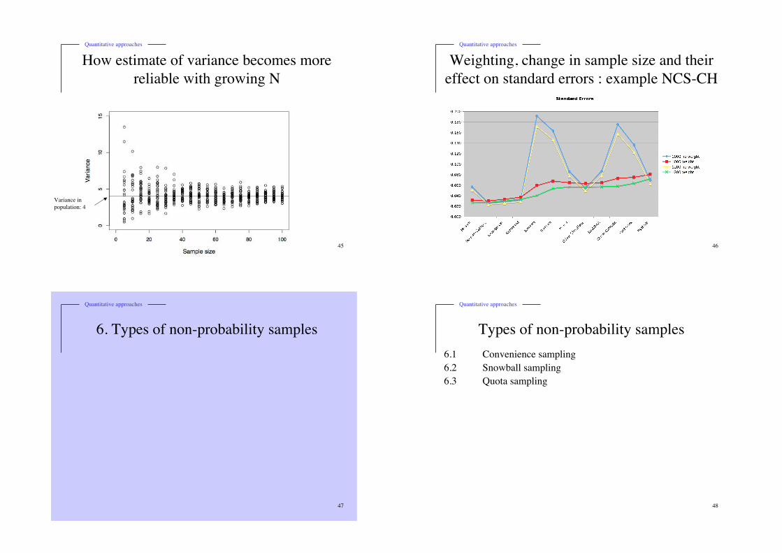
How estimate of variance becomes more

reliable with growing N

Variance in

population: 4

46


Weighting, change in sample size and their

effect on standard errors : example NCS-CH

47


6. Types of non-probability samples

48


Types of non-probability samples

6.1 Convenience sampling

6.2 Snowball sampling

6.3 Quota sampling

49


6.1 Convenience sampling

Convenience sampling

= We choose the people who are most easily available /approachable.

Problem:

We do not know for what population these people arerepresentative / whom they stand for

50


Convenience sampling: example

"Nous avons déposé dans les boîtes aux lettres des enseignants - qui existent dansla plupart des universités - le questionnaire, une note explicative du contenu denotre recherche, et une enveloppe avec notre adresse afin qu'ils puissent nousfaire parvenir le questionnaire dûment rempli.

La plupart des universités parisiennes - ainsi qu'un bon nombre des plusimportants centres de recherche - sont inclus dans notre enquête. Nous avonsdéposé des questionnaires à Paris I, Paris II, Paris III, Paris V, Paris VI, Paris VII,Sauphine, Paris X-Nanterre, Paris VIII, l'Institut de Sciences Politiques, laMaison des Sciences de l'Homme, et l'Ecole Normale Supérieure.

271 enseignants nous ont fait parvenir leurs réponses au questionnaire.Cependant, les 271 réponses ne constituent pas un échantillon représentatif quipermette de décrire les caractéristiques générales de la population desenseignants. Par exemple, il ne nous permet pas de déterminer le pourcentaged'individus qui sont séduits pour les positions de gauche. L'échantillon n'est doncconstruit que pour fournir un test et non pour décrire la population desenseignants parisiens.

(Magniberton/Rios, 2003)

51


6.2 Snowball sampling

Snowball sampling = We ask the first participants for addresses of other individuals who havethe same characteristics. Every participant is again asked for still otherparticipants.

Problem: no representativity

52


Snowball sampling: example

"I conducted fifty interviews with marijuana users. I hadbeen a professional dance musician for some years when Iconducted this study and my first interviews were withpeople I had met in the music business. I asked them to putme in contact with other users who would be willing todiscuss their experiences with me... Although in the end halfof the fifty interviews were conducted with musicians, theother half covered a wide range of people, includinglaborers, machinists, and people in the professions(Becker 1963: 45-6)

53


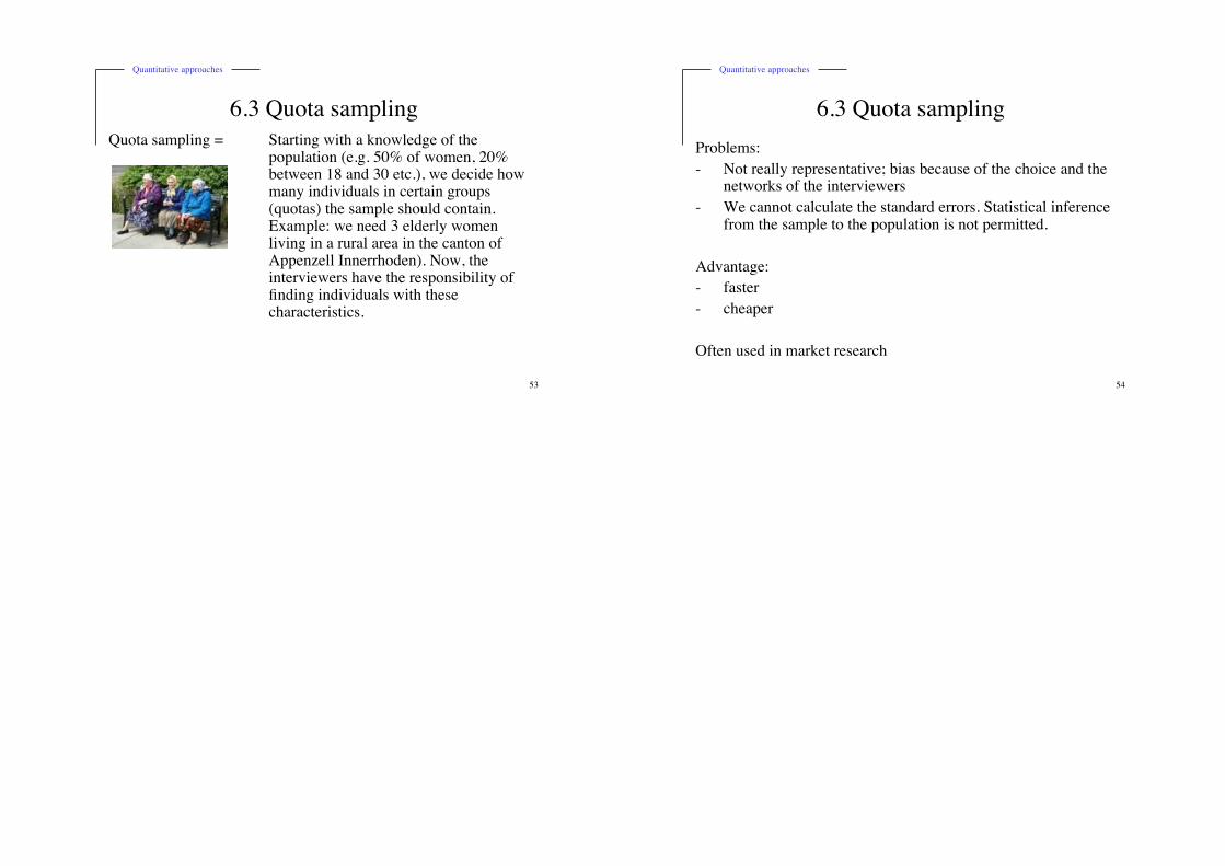
6.3 Quota sampling

Quota sampling = Starting with a knowledge of the population (e.g. 50% of women, 20%between 18 and 30 etc.), we decide howmany individuals in certain groups(quotas) the sample should contain.Example: we need 3 elderly womenliving in a rural area in the canton ofAppenzell Innerrhoden). Now, theinterviewers have the responsibility offinding individuals with these characteristics.

54


6.3 Quota sampling

Problems:

- Not really representative; bias because of the choice and thenetworks of the interviewers

- We cannot calculate the standard errors. Statistical inferencefrom the sample to the population is not permitted.

Advantage:

- faster

- cheaper

Often used in market research