Download pdf - Optimal taxation with endogenously incomplete debt markets

Journal of Economic Theory 127 (2006) 36–73www.elsevier.com/locate/jet

Optimal taxation with endogenously incompletedebt markets�

Christopher Sleeta, Sevin Yeltekinb,∗aDepartment of Economics, University of Iowa, Iowa City, IA 52242, USA

bMEDS, Kellogg School of Management, Northwestern University, 2001 Sheridan Road, 5th Floor, Evanston,IL 60208, USA

Received 9 January 2004; final version received 30 July 2004Available online 23 November 2004

Abstract

Empirical analyses of labor tax and public debt processes provide prima facie evidence for im-perfect government insurance. This paper considers a model in which the government’s inability tocommit to future policies or to report truthfully its spending needs renders government debt marketsendogenously incomplete. A method for solving for optimal fiscal policy under these constraints isdeveloped. Such policy is found to be intermediate between that implied by the complete insurance(Ramsey) model and a model with exogenously incomplete debt markets. In contrast to optimalRamsey policy, optimal policy in this model is consistent with a variety of stylized fiscal policy factssuch as the high persistence of labor tax rates and debt levels and the positive covariance betweengovernment spending and the value of government debt sales.© 2004 Elsevier Inc. All rights reserved.

JEL classification: D82; E62; H21

Keywords: Optimal taxation; Fiscal policy; Dynamic contract theory

� We thank two anonymous referees for many useful suggestions. We thank seminar participants at Duke, UCLA,Illinois Urbana-Champaign, Northwestern, the Cleveland and Richmond Feds, the 2003 SED Meetings and SITEfor their comments.

∗ Corresponding author. Fax: +1 847 467 1220.E-mail address: [email protected] (S. Yeltekin).

0022-0531/$ - see front matter © 2004 Elsevier Inc. All rights reserved.doi:10.1016/j.jet.2004.07.009

http://www.elsevier.com/locate/jet

mailto:[email protected]

C. Sleet, S. Yeltekin / Journal of Economic Theory 127 (2006) 36–73 37

1. Introduction

This paper considers the optimal design of fiscal policy under two sets of restrictions.The first set is exogenous; it describes the technology by which the government can extractresources from agents. We follow the conventional Ramsey approach and suppose thatresources can be obtained by levying linear taxes or selling state contingent debt. We alsoassume that the government cannot lend. The second set of restrictions stem from incentiveproblems on the side of the government which we assume can neither commit to repayingits debt nor to truthfully revealing private information about its spending needs. Thesefrictions impede the government’s ability to use asset markets to hedge fiscal shocks. Theyendogenously restrict the set of asset trades the government can make and this, in turn, hasimplications for the optimal setting of taxes. To analyze fiscal policy design in such settings,we embed the government’s policy problem into a repeated game.We provide an equilibriumconcept that extends Chari and Kehoe’s [15,16] sustainable equilibrium to environmentswith private government information. We then give necessary and sufficient conditions foran allocation to be an equilibrium outcome of this game. These conditions are recursive andwe obtain a dynamic programming method for finding optimal equilibrium allocations thatexploits this recursivity. We back out the supporting fiscal policies from these allocations andanalyse optimal fiscal policy in this limited commitment-private information environment.

Our immediate motivation is a contrast between the benchmark Ramsey model of fiscalpolicy (as developed by Lucas and Stokey [22]) and the data. The former implies that fiscalpolicy variables should depend only upon the current realization of the shocks perturbing theeconomy and, consequently, should inherit their stochastic properties from these shocks. Incontrast, empirical evidence on labor tax rates and the public debt suggest that these variablesexhibit considerable persistence, much more than that for government spending and othercandidate shock processes. 1 To paraphrase Aiyagari, Marcet, Sargent and Seppälä (AMSS)[2], the empirical labor tax rate process is smooth in the sense of being highly persistent,rather than smooth in the sense of having a small variance.

The data are suggestive of considerable intertemporal, but limited interstate smoothingof taxes. Thus, they provide prima facie evidence for incomplete government insurance.The papers of AMSS, Marcet and Scott [23] and Scott [27], which assume exogenouslyincomplete government debt markets, corroborate this view and suggest that a limited abilityto hedge against fiscal shocks may have significant implications for the design and conductof fiscal policy. Given this, it becomes important to understand why this ability is limitedand in what circumstances it might be more or less restricted.

Many commentators have informally suggested that moral hazard problems of one sortor another might underpin incomplete government insurance (e.g. [9,10,25]). The privateinformation and limited commitment frictions that we incorporate into our model formalizethese ideas. Both are linked to familiar time consistency considerations. The repayment ofdebt requires the levying of distortionary taxes. Ex post the government, and all households,would be better off if the debt were cancelled, but if such cancellation is anticipated ex ante,

1 Marcet and Scott [23] show that even after capital, which is absent from the Lucas and Stokey model, isincorporated, the empirical processes for fiscal variables remain too persistent relative to those implied by theRamsey model.

38 C. Sleet, S. Yeltekin / Journal of Economic Theory 127 (2006) 36–73

the government will be unable to sell any debt in the first place. Our model gives thegovernment two channels via which it can avoid making debt repayments. The first is anoutright repudiation of the debt. The second is more subtle; the government may exploitthe private information it has over its spending needs and the state contingency of debtrepayments to obtain a reduction in the latter. If, in order to smooth taxes, it has sold moreclaims against low relative to high spending needs states, the government can reduce itsdebt repayment by claiming its spending needs are high when they are really low. 2

We call allocations that can be supported as equilibrium outcomes of our game “sus-tainable incentive-compatible competitive allocations” (SICCA’s). Our main focus is uponSICCA’s that are optimal from the government’s point of view. We show that optimalSICCA’s are recursive in the value of the government’s debt. The limited commitment con-straint translates into an upper bound on equilibrium debt values. Above this upper bound,the government cannot be given incentives to repay its debt. It is the fiscal policy analogueof the endogenous solvency constraints that Alvarez and Jermann [3] find in a model ofhouseholds who are unable to commit ex ante to making debt repayments. There is also alower debt value limit that stems from our assumption that the government cannot lend. Inmaking this last assumption, we follow Chari and Kehoe [15]. We elaborate on its role andits justification in Section 3.

Our recursive method allows us to jointly solve for the debt value limits and for thegovernment’s optimal equilibrium payoff as a function of its current debt value. The methodis related to the approach of Abreu, Pearce and Stacchetti (APS) [1] and to the recentextensions of this approach to macroeconomic policy games provided by Chang [12], Phelanand Stacchetti [26] and Sleet [28]. We show that the government’s value function satisfies aBellman equation on the set of debt values that lie between the limits. The policy functionsfrom this dynamic programming problem can be used to recursively construct optimalallocations and, hence, optimal fiscal policy. This policy has the following characteristics.Away from the debt value limits, it exhibits considerable intertemporal tax smoothing, amoderate degree of state contingency in debt returns and considerable persistence in bothtaxes and debt. These features are consistent with the empirical analyses of Bizer and Durlauf[8], Huang and Lin [20] and Kingston [21] (on taxes) and Marcet and Scott [23] (on debt).Close to the limits, there is much more volatility in tax rates.

The limited commitment, no lending and incentive compatibility frictions interact ininteresting ways. In a model with only the incentive compatibility friction, tax rates andthe excess burden of taxation tend to drift upwards over time. Sleet [29] shows that, undercertain assumptions on preferences, this drift continues until the government is maximallyindebted. At this point, it maximizes and uses all of its tax revenues to service debt. Theseverity of this outcome raises natural questions about the government’s ability to committo implementing it ex ante. The endogenous upper debt value limit that stems from thecommitment friction arrests the drift before this severe outcome is attained. Moreover, boththe limited commitment and no lending frictions aggravate the incentive problem, especiallywhen the government’s debt value is close to the debt value limits. This contributes to thegreater tax rate volatility in these regions.

2 The private information friction is less familiar than the limited commitment one. We provide an extendedmotivation for it in Section 3.


In a model with only the no lending and commitment frictions, such as that of Chariand Kehoe [15], debt value limits are also present. As Chari and Kehoe show, there isa reduced scope for fiscal hedging and a motive for intertemporal smoothing of taxes inthe neighborhood of these limits. The addition of the incentive constraints further restrictsthe government’s ability to hedge fiscal shocks and creates a motive for intertemporal taxsmoothing across the whole debt value domain. Overall, numerical calculations indicate thatthe three frictions result in a constrained optimal fiscal policy with properties somewherebetween those implied by the Ramsey model and a model with non-contingent debt andexogenously set debt limits. Corroborative evidence reported by Marcet and Scott [23]suggests that empirical fiscal policies are also somewhere between these benchmarks.

Our model is related to two recent contributions, Athey, Atkeson and Kehoe (AAK)[5] and Sleet [28], that have considered optimal monetary policy under private governmentinformation. InAAK’s model the private information concerns the government’s preferencesfor inflation and the government implements policy contingent on the history of reports thatit has made concerning its attitude towards inflation. A key result of AAK is that optimalmonetary policy is in fact static and does not respond to past reports. Although our modelshares some of the same structure as AAK’s, we find that optimal fiscal policy is not static.

Finally, Angeletos [4] presents an alternative decentralization of benchmark Ramseyallocations that relies upon non-contingent debt of varied maturities and a state contingentfiscal policy. It is important to emphasize that even though explicitly state contingent debtis absent from this model, the decentralization proposed by Angeletos does not immunizethe government from the frictions analyzed in this paper. In particular, if a governmentis privately informed about its spending needs, implementation of the Ramsey allocationunder this alternative arrangement would still require it to condition its policies on thisinformation. This would create an opportunity and an incentive for such a government tomisrepresent its spending needs in order to justify alternative policy actions.

The outline for the remainder of the paper is as follows. Section 2, describes the bench-mark environment with full commitment and without private information. Section 3, thenintroduces the incentive compatibility, limited commitment and no lending frictions andreformulates the model in game-theoretic terms. The next section provides a recursive for-mulation of the optimal SICCA that is amenable to computation. In particular, this sectionshows how limited commitment constraints can be recast as debt value limits. Section 5,gives a partial theoretical characterization of optimal SICCA’s, while Section 6 providesillustrative numerical calculations.

2. The benchmark environment

The benchmark Ramsey environment is characterized by complete information and fullcommitment on the part of the government. The economy is inhabited by a governmentand a continuum of identical households, all assumed to be infinitely lived. Taste shocksto the government’s and, under some interpretations, society’s preference for public goodsare the underlying source of uncertainty. Denote the associated shock process by �∞ ={�t }∞t=0, with each �t ∈ � ≡ {�1, . . . , �N }, �i+1 > �i . Assume that each �t is distributed

i.i.d. with probability distribution P = {P(�i )}Ni=1 ∈ RN++. Denote histories of shocks


(�0, . . . , �t ) ∈ �t+1 by �t and the probability distribution over such a history by P t(�t ). Ahousehold allocation gives the consumption ct , and labor supply lt of a household at each tand conditional on all possible �t . An allocation augments this with a sequence of functionsg∞ = {gt }∞t=0 that gives government spending at each date and after all histories.

Definition 1. A household allocation is a collection of functions eh∞ = {ct , lt }∞t=0 with,for each t, ct : �t → R+ and lt : �t → [0, T ]. A household allocation is interior if for allt, �t , ct (�

t ) > 0 and lt (�t ) ∈ (0, T ).

An allocation is a collection of functions e∞ = {ct , lt , gt }∞t=0 with {ct , lt }∞t=0 a householdallocation and for each t, gt : �t → R+. An allocation {ct , lt , gt }∞t=0 is interior if {ct , lt }∞t=0is an interior household allocation. Let � denote the set of interior allocations.

Households value household allocations according to V h(eh∞) = E[∑∞

t=0 �tU(ct , lt )],

with � ∈ (0, 1), and U(c, l) = u(c) + y(l), where

u(c) ={

c1−�

1−� � ∈ (0, 1),

ln c � = 1,y(l) =

{(T −l)1−�

1−� � ∈ (0, 1),

ln(T − l) � = 1.(1)

The arguments given below can be easily extended to the case � = 0. To economize onspace they are omitted. There is a linear production technology that converts one unit oflabor supply into one unit of output. In each period, households can trade claims contingenton the next period’s shock realization.

A fiscal policy is a collection of functions x∞ ≡ {st , St , �t , qt }∞t=0. Here, st : �t → [0, 1],St : �t → R+ and �t : �t → (−∞, 1) denote, respectively, a tax on claim payouts, alump sum transfer and a labor income tax set by the government at t as a function of thehistory of shocks. qt : �t+1 → R+ is a pricing kernel, set by the government at t aftereach �t , for one period ahead claims contingent on �t+1. The government supplies claimson demand at these prices. Let Qs

t = ∏sr=1

[qt+r−1/(1 − st+r )

], s�1, Q0

t = 1, denote theafter-tax price of a unit of consumption at date t + s in terms of date t consumption. Letbt+1(�

t , �t+1) denote the quantity of �t+1-contingent claims purchased by the householdat t after �t , and define at (�

t ) ≡ (1 − st (�t ))bt (�

t )+St (�t ). Finally, define the household’s

natural debt limit at t after history �t as

At(�t ) =

∞∑s=0

∑�s∈�s

Qst (�

t , �s)[(1 − �t+s(�

t , �s))T + St+s(�t , �s)

].

At (�t ) gives the maximal amount a household can afford to repay after �t . We assume that

the fiscal policy satisfies −(1 − s0(�0))b0(�

0) < A0(�0) < ∞ and is such that {At }∞t=0 is

well defined and real-valued.A household plan is a pair

{eh∞, b∞}, where b∞ = {bt+1}∞t=0 denotes a sequence of

claim holdings. Given an initial portfolio of claims b0 and a fiscal policy x∞, the householdchooses such a plan to solve

sup{eh∞,b∞}

E

[ ∞∑t=0

�tU(ct , lt )

](2)


subject to:

∀t, �t , at (�t )�ct

(�t)− (1 − �t (�

t ))lt(�t)+

∑�∈�

qt (�t , �)bt+1(�

t , �),

∀ t, �t , �t+1, (1 − st+1(�t+1))bt+1(�

t , �t+1)� − At+1(�t , �t+1).

Definition 2. A household plan{eh∞, b∞}, fiscal policy x∞, sequence of government

spending functions g∞, and an initial household portfolio b0 is a competitive equilibrium,if (i)

{eh∞, b∞} solves the household’s problem given x∞ and b0, (ii) x∞,

{eh∞, b∞}, and

g∞ satisfy the government’s budget constraints: 3

∀t, �t : at (�t ) + gt (�

t )��t (�t )lt (�

t ) +∑�∈�

qt (�t , �)bt+1(�

t , �). (3)

e∞ = {ct , lt , gt }∞t=0 is a competitive allocation if it is part of a competitive equilibrium.

Define J (c, l) = �U

�c(c, l)c + �U

�l(c, l)l so that under the preferences in (1), J (c, l) =

c1−� − l(T −l)�

. In a competitive equilibrium, the budget constraints of the household and

government and the household’s first order conditions imply J (ct , lt ) = c−�t (ct − (1 −

�t )lt ) = c−�t (�t lt −gt ). Hence, J (ct , lt ) gives the government’s primary surplus in marginal

utility of consumption terms. Let Jc and Jl denote the derivatives of J with respect toconsumption and labor supply.

2.1. Debt values and competitive equilibria

Given a competitive equilibrium {e∞, b∞, x∞}, we can define the sequence of functions

{�t }∞t=0 pointwise as follows: �0 = E[(1 − s0)b0c

−�0

]and for each t �0, �t , �t+1(�

t ) =E�t

[(1 − st+1)bt+1c

−�t+1

]. Thus, �t+1(�

t ) denotes the expected value of the household’s

time t + 1 portfolio in marginal utility of consumption terms, conditional on information att. We refer to �t as a debt value. A particular competitive allocation may be part of manydifferent competitive equilibria, each distinguished by a different sequence of debt holdingsand lump sum transfers. This motivates the following definition.

Definition 3. A sequence of debt values {�t }∞t=0, �0 ∈ R and, t �0, �t+1 : �t → R, isconsistent with a competitive allocation e∞ = {ct , lt , gt }∞t=0 ∈ � if there exists a com-petitive equilibrium {e∞, b∞, x∞} with taxes on claim payouts {st }∞t=0 such that �0 =E[(1 − s0)b0c

−�0

]and ∀t �0, �t , �t+1(�

t ) = E�t

[(1 − st+1)bt+1c

−�t+1

].

The next proposition provides necessary and sufficient conditions for an interior allocationto be competitive. It formalizes the link between competitive allocations and debt values.

3 We do not separately impose a No Ponzi condition on the government. Instead, we rely on the transversalitycondition from the household’s problem to ensure: limt→∞

∑�t+1∈�t+2 Qt

0(�t , �t+1)bt+1(�t , �t+1)�0.


Proposition 1. e∞ = {ct , lt , gt }∞t=0 ∈ � is a competitive allocation if and only if thereexists a sequence �∞ = {�t }∞t=0, with �0 ∈ R and, for t �0, �t+1 : �t → R, such that e∞and �∞ satisfy:

1. (Recursive implementability) �0 �E[J (c0, l0) + ��1

], ∀t �1, �t−1

�t (�t−1)�E�t−1

[J (ct , lt ) + ��t+1

], (4)

and limr→∞ �rE�t−1[�t+r

] = 0;2. (Resource constraints) ∀t, �t , lt (�

t ) − ct (�t ) − gt (�

t )�0.

Moreover, �∞ is a consistent sequence of debt values for e∞.

Proof. See [30]. �Eq. (4) provides a recursive version of the standard Ramsey implementability condition

(see [17]). It is obtained by substituting prices and taxes out of the household’s budgetconstraint using the first order conditions from the household’s choice problem. Addition-ally, the inclusion of lump sum transfers relaxes (4) to an inequality. 4 Given an allocationsatisfying the conditions of the proposition, the household’s first order conditions can beused to pin down the associated competitive equilibrium labor tax rates and after-tax assetprices.

Let E(�) denote the set of (interior) competitive allocations that are part of a competitiveequilibrium with initial debt value equal to �. Proposition 1 implies that competitive alloca-tions are recursive. Specifically, if {�t }∞t=0 is consistent with e∞ ∈ �, then after any �t , thecontinuation of e∞, e∞|�t = {

ct+r (�t , ·), lt+r (�

t , ·), gt+r (�t , ·)}∞

r=1, is itself a competitiveallocation belonging to E(�t+1(�

t )). The following lemma establishes the existence of a

natural debt value limit, �nat

: an upper bound on debt values. Later on we will imposeadditional frictions that tighten this limit.

Lemma 1. Let {�t }∞t=0 be a sequence of debt values consistent with some competitiveallocation, then

∀t, �t , �t (�t )��

nat ≡ supl∈[0,T ]

1

1 − �J (l, l) < ∞.

For all � ∈ (−∞, �nat], E(�) �= �.

Proof. See [30]. �Define C(�) equal to all {c, l, g, �′} such that:

��∑�∈�

[J (c (�) , l (�)) + ��′(�)],

4 This relaxation ensures that the set of competitive allocations with a fixed initial debt value is convex, a factused later.


l(�) − c(�) − g(�)�0,

c(�)�0, g(�)�0, l(�) ∈ [0, T ], �′(�) ∈ (−∞, �nat].

Then, it is immediate that any competitive allocation {ct , lt , gt }∞t=0 satisfies, for all t, �t−1 andconsistent debt value sequence {�t }∞t=0, {ct (�

t−1, ·), lt (�t−1, ·), gt (�t−1, ·), �t+1(�

t−1, ·)} ∈C(�t (�

t−1)). Conversely, any allocation constructed by choosing �0 ∈ (−∞, �nat] and

then successively selecting {ct (�t−1, ·), lt (�

t−1, ·), gt (�t−1, ·), �t+1(�

t−1, ·)} ∈ C(�t

(�t−1)) is a competitive allocation.

2.2. Government preferences and the Ramsey solution

The government values allocations according to

V g(e∞) = E

[ ∞∑t=0

�tW(ct , lt , gt ; �t )

], (5)

where W(ct , lt , gt ; �t ) = U(ct , lt ) + �tgt

1−1− and > 0. As in many analyses of optimal

taxation, the welfare of the representative household enters the government’s preferences.The second term in the above expression for W may be interpreted as the utility privateagents receive from the provision of public goods, or as the utility the government receivesfrom its own consumption. In either case, the taste shock �t alters the weight placed on thissecond term in the government’s preferences. In this paper, we study policy that is optimalfor the government. However, under the first interpretation, it is optimal for the householdas well.

We assume that the government receives an initial debt value �0 and then selects acompetitive allocation from E(�0) to solve:

V R(�0) = supe∞∈E(�0)

V g(e∞).

We call this the Ramsey problem. 5 To facilitate comparison with later sections, we providea brief overview of this problem and of its solution. Proofs of the results given below followfrom arguments in [17,23,31] and are omitted.

Applying standard arguments, the Ramsey problem can be reformulated recursively.

Specifically, V R : (−∞, �nat] → R is the unique bounded, continuous solution to the

functional equation:

V R(�) = sup{c,l,g,�′}∈C(�)

∑�∈�

[W(c(�), l(�), g(�); �) + �V R(�′(�))]P (�) . (6)

5 The conventional Ramsey problem fixes b0 rather than �0. In subsequent periods, however, the governmentcan be modelled as acting as if it has inherited a debt value from the past. In contrast, we treat the first periodsymmetrically with later periods and think of the government as committed to a �0.


Let {cR, lR, gR, �R} denote the (unique) policy functions that solve the optimizations in(6). Given an initial debt value, �0, these policy functions induce a Ramsey allocation,eR(�0), according to cR

t (�t ) = cR(�Rt (�t−1), �t ), lRt (�t ) = lR(�R

t (�t−1), �t ), gRt (�t ) =

gR(�Rt (�t−1), �t ), where �R

t+1(�t ) = �R(�R

t (�t−1), �t ) and �R0 (�−1) = �0. Let �R :

[0, �nat] → R+ denote the Lagrange multiplier on the recursive implementability con-

straint in this problem. We call an allocation {ct , lt , gt }∞t=0 static if there exist functionsc : � → R+, l : � → [0, T ] and g : � → R+ such that ∀t, �t−1, �, ct (�

t−1, �) = c(�),lt (�

t−1, �) = l(�), and gt (�t−1, �) = g(�). Otherwise, we call it dynamic.

Proposition 2. The Ramsey allocation is static. For all �, �, �R (�, �) = �.

To ensure that the Ramsey competitive equilibrium associated with eR(�0) is uniquelydetermined, we assume that for all t, �t , st (�

t ) = 0 and St (�t ) = 0. The household’s first

order conditions can then be used to obtain the remaining variables that comprise this com-petitive equilibrium as functions of {cR

t } and {lRt }. The static nature of the Ramsey allocationthen implies that after each �t , the tax rate �t (�

t ), quantity of claims outstanding, bt (�t )

and revenues raised from new claim sales∑

� qt (�t , �)bt+1(�

t , �) are given by functions�R(�0, �t ), bR(�0, �t ) and dR(�0, �t ), respectively. The following proposition characterizesthe implications of the Ramsey allocation for tax policy and debt management.

Proposition 3. The functions �R , bR and dR satisfy the following conditions.

1. �R(�0, �) ≡�R(�0)

(1 − (1−�)

�(lR(�0,�))

)�R(�0) + 1

�(lR(�0,�))

, (7)

where �(l) = 1 + �l/(T − l), or one plus the Frisch elasticity of labor supply.2. If � < �, then bR(�0, �) > bR(�0, �).3. If � < �, then dR(�0, �) > dR(�0, �).

�R(�t (�t−1)) gives the multiplier on the implementability constraint after history �t−1.

It can be interpreted as the excess burden of taxation. Since �t remains constant at �0,�R(�t (�

t−1)) remains constant as well. This is the key sense in which Ramsey policy“smooths”; its implications for taxes are captured in (7). Since �R is constant, taxes onlyvary in so far as the Frisch elasticity of labor supply, �(l), varies across states. In contrast,if the government operated under a balanced budget rule, it would face a sequence of staticimplementability constraints of the form: J (ct (�

t ), lt (�t )) = 0. The multipliers on these

constraints would fluctuate across states of nature and would impart additional volatility totax rates beyond that implied by variations in �(l).

The second and third items in Proposition 3 describe two key aspects of optimal debtmanagement. First, the government sells fewer claims against high � states and more againstlow � states. In this way it hedges � risk. Second, during high spending periods, the price ofclaims is low and this reduces the amount the government raises from selling the portfolio{bR(�0, ·)}.


3. Environments with private information and limited commitment

We now consider altering the environment of the previous section by introducing threeextra frictions. First, we assume that the government has a limited ability to commit toimplementing future policies. Second, we suppose that the government privately observesthe taste shocks {�t }. Finally, we assume that the government cannot lend, so that in equi-librium, ∀t , �t , bt (�

t )�0. We formalize the first two frictions below and show that theylead to endogenous restrictions on the set of asset trading strategies available to the gov-ernment. The third friction represents a direct exogenous restriction on asset trades. Beforeproceeding, we motivate the less familiar private government information and no lendingfrictions.

Throughout the remainder of the paper, we use the assumption that the {�t } shocks areobserved only by the government as a simple way of capturing the more general ideathat the government has private information concerning its spending needs. 6 We have inmind one of two situations. In the first, the government extracts resources for its own endsand its spending needs are imperfectly observable. In the second, private households areheterogenous in their taste for public goods. They may be well informed about their owntastes or the appropriate level of public good provision in their locality, but less informedthan the government about the average need, as represented by �. Alternatively, privatehouseholds with different attitudes towards public goods provision may not know the extentto which the government, both in the current and in future periods, weights their variedpreferences. Its weighting scheme may be subject to publicly unobservable shocks.

There may be many other potential sources of private government information. Suchsources might include privately observed shocks to the technology for producing publicgoods, private information about the desirability of public investments (e.g. in militaryhardware or in wars themselves) and, if taxes are set before spending needs shocks are re-alized, private forecasts of spending needs shocks. Our formulation of private governmentinformation seems the simplest amongst these. However, we conjecture that the incorpo-ration of these alternative sources of private government information would lead to resultsqualitatively similar to ours.

It is worth noting that there is a tradition of analyzing privately informed policy makersin the monetary policy literature. Many of the situations considered in this literature par-allel those described above. Specifically, Athey et al. [5], Barro [7] and Cuckierman andMeltzer [18] consider environments in which a central bank has private information aboutits preferences, while Canzoneri [11] and Sleet [28] consider ones in which the governmenthas private information about the state of the economy.

We regard the no lending friction as a simple, if strong, way of capturing the costs anddistortions associated with enforcing the repayment of loans to the government. Chari andKehoe [15] motivate such a friction by supposing that private household asset trades areanonymous so that claims held against them are unenforceable. More generally, we think

6 We assume private information concerning the government’s spending needs rather than government spendingitself.Although it is reasonable to assume that the former is less observable than the latter, several recent papers havedocumented how governments seek to obscure their spending levels through various forms of creative accounting,suggesting that even spending levels may not be perfectly observed. See, in particular, [24].


Period t+1Period t

tt gx ~,~menu

announcesGovernment

government

torevealedtθ

esasset tradundertakes

and taxesimplements

,~

announcesGovernment tδ

consumeandassetstrade

pay taxes,Households

Fig. 1. Time line.

that transfers from households to the government, whether loan repayments or taxes, shouldbe treated symmetrically. Unless loans from the government are collateralized, then, liketaxes, loan repayments should depend upon the household’s current labor income and,hence, will be distortionary. Technically, the no lending constraint will reduce the payoffassociated with the worst equilibrium in the game we construct below. This, in turn, willallow a larger set of fiscal policies to be supported in equilibrium.

3.1. The policy game

To analyze fiscal policy in the presence of the frictions described above, we embed thegovernment’s problem into a policy game. The timing of moves in the game is illustratedin Fig. 1. The government enters period t with a portfolio of bonds bt ∈ RN+ . These bondsare claims to a unit of consumption contingent on a taste shock report that the governmentmakes later in the period. Before any shocks are realized, the government selects a menuof taxes and debt prices, xt = {st , �t , St , qt }, and a menu of government spending levels,gt . Here st : � → [0, 1] , �t : � → (−∞, 1), St : � → R+, qt : � → RN+ andgt : � → R+ give the current tax on debt, labor tax rate, lump sum subsidy, vector of bondprices and government spending level respectively, all contingent on the report made by thegovernment. We denote the set of possible tax and debt price menus by X and refer to a pair{xt , gt } as a fiscal menu.

Next, the government privately observes the current shock �t and makes a report t

concerning its value. It then implements the appropriate item from the fiscal menu,{st ( t ), �t ( t ), St ( t ), qt ( t ), gt ( t )}. Having observed {xt , gt } and the report t , privateagents make their choices ct , lt and their bond purchases, bt+1. The government stands byready to supply any non-negative quantity of bonds at the prices it has previously set. Thesetiming assumptions incorporate a degree of commitment on the part of the government;once it has chosen a fiscal menu, it is committed to making a selection from this menu afterobserving �. Within a period, the menu gives the government some discretion in respondingto shocks. However, the government is unable, at time t, to commit to implementing futurefiscal menus or to making specific shock-contingent reports. In particular, entering a period,the government may be tempted to implement a new menu with higher taxes on outstandingdebt (an observable default), or, having observed the state, alter its report and misrepresentits true taste shock so as to obtain a reduction in its outstanding liabilities (a hidden default).

Define a t-period public history, ht , to be a list of past policy actions taken and reportsmade by the government: ht = {b0, {xr , gr , r}t−1

r=0}, t �1 and h0 = {b0}. Given an initial


portfolio b0 ∈ RN+ , let Ht = {b0} × (X × RN+ × �)t denote the set of t-period publichistories. Note that an element of Ht describes the history of the economy at the beginningof period t before the government acts. Private agents take their actions after the governmentso that their period t behavior is conditioned on ht+1. A t-period private government history,h

gt ∈ H

gt = Ht × �, augments ht with the most recent shock realization, �t .

A government strategy is a collection of functions, �g = {�gt }∞t=0, that describes the

government’s policy actions after each hgt . �g

t has three components: a pair of fiscal menufunctions x�

t : Ht → X, and g�t : Ht → RN+ , and a report function �

t : Hgt → �,

with �gt (ht , �t ) = (x�

t (ht ), g�t (ht ),

�t (ht , �t )). Thus, we restrict attention to government

strategies that condition on public histories and the most recent realization of the privateshock, but not on the entire history of private shocks. 7 Let ht (�g, �t−1) be the t-periodpublic history induced by �g and the sequence of shocks �t−1. Any strategy, together withthe process for shocks, induces a probability distribution over public histories. Let E�g

denote the expectations operator associated with this probability distribution.An allocation profile �h = {�h

t }∞t=0, with �ht = {

c�t , l�t , b�

t+1

}, describes the consumption,

labor supply and bond holding choices of households contingent on the realization of publichistories. Thus, c�

t : Ht+1 → R+, l�t : Ht+1 → R+ and b�t+1 : Ht+1 → RN+ . Let

�g|ht ={x�t+j (ht , ·), �

t+j (ht , ·)}∞

j=0and �h|ht+1 =

{c�t+j (ht+1, ·), l�t+j (ht+1, ·), b�

t+1+j

(ht+1, ·)}∞

j=0. A strategy-allocation profile

(�g, �h

)and an initial b0 induce an outcome

allocation and an outcome fiscal policy.

Definition 4. A sequence of functions {xt , t , gt , ct , lt , bt+1}∞t=0 is an outcome of a strategy-allocation profile, � = (�g, �h) = {

x�t , g�

t , �t , c�

t , l�t , b�t+1

}∞t=0, and initial b0 ∈ RN+ if

h0 = b0 and for each �t ,

1. xt (�t ) = x�

t (ht (�g, �t−1), �t (ht (�g, �t−1), �t )),

2. gt (�t ) = g�

t (ht (�g, �t−1), �t (ht (�g, �t−1), �t )),

3. t (�t ) = �

t (ht (�g, �t−1), �t ),4. ct (�

t ) = c�t (ht+1(�g, �t )),

5. lt (�t ) = l�t (ht+1(�g, �t )),

6. bt+1(�t ) = b�

t+1(ht+1(�g, �t )).

Call the allocation {ct , lt , gt }∞t=0 obtained in this way the outcome allocation of �. Call{xt }∞t=0 the outcome fiscal policy of � and { t }∞t=0 the outcome reporting policy of �. Finally,call {ct , lt , bt+1}∞t=0 the outcome household plan of �.

We will refer throughout to a profile of functions { t }∞t=0, t : �t+1 → �, as a reportingpolicy. Finally, let V

gt (�g, �h|ht ) denote the payoff to a government from a pair (�g, �h)

after a history ht .

7 In doing so we follow other contributions to the literature, e.g. [5]. The exclusion of past private agent actionsfrom public histories is justified by arguments in [14].


3.2. Sustainable equilibria and allocations

A sustainable equilibrium of the policy game is a strategy-allocation profile (�g, �h) thatis consistent with household optimality and market clearing, and a sequential rationalityrequirement on �g . The latter necessitates that, after each history, the government is betteroff adhering to �g than deviating to some feasible alternative strategy. Consequently, beforegiving a formal statement of an equilibrium, it is necessary to define the set of deviationsavailable to a government. Within a period there are two sorts of feasible deviation. Atthe beginning of the period, the government can implement a fiscal menu different fromthat prescribed by its strategy. Later, after receiving the shock, it can deviate by altering itsreport. It is always free to give any report it wishes. However, it may only deviate to budgetfeasible fiscal menus.

Definition 5. A fiscal menu (x, g) is budget feasible at ht under � if for each ∈ �,

�( )l�t (ht , x, g, ) +∑ ′∈�

q( , ′)b�t+1(ht , x, g, , ′)

� g( ) + (1 − s( ))b�t (ht , ) + S( ).

Definition 6. Given a strategy-allocation profile � = (�g, �h

), �g is a feasible deviation

for the government if for all ht , the fiscal menu induced by �g , (x�t (ht ), g

�t (ht )), is budget

feasible at ht under �.

Let x(�g)|ht+1 denote the outcome fiscal policy induced by a government strategy �g

after ht+1. Similarly, let{eh∞, b∞} (�)|ht denote the outcome household plan induced

by a strategy-allocation profile �. The formal statement of a sustainable equilibrium nowfollows.

Definition 7. A sustainable equilibrium at �0 is a triple (b0, �g, �h) with b0 ∈ RN+ , �g ={x�t , g�

t , �t

}∞t=0 and �h = {

c�t , l�t , b�

t+1

}∞t=0 that satisfies the following conditions.

1. Competitive equilibrium.(a) After all histories ht+1 = (ht , s, S, �, q, g, ), given the household’s current claim

holdings b�t (ht ), the current policy {s, S, �, q, g, } and the continuation outcome

fiscal policy x(�g)|ht+1, the outcome plan{eh∞, b∞} (�)|ht maximizes the house-

hold’s utility subject to its budget constraints and debt holding limits.(b) The functions

{b�t+1

}∞t=0 satisfy, for all t �0, ht+1, t+1, b�

t+1(ht+1, t+1)�0.

(c) At each ht , (x�t (ht ), g

�t (ht )) is budget feasible.

(d) �0 = E�g[(

c�0

)−�(1 − s�

0 )b0

].

2. Government optimality. For all ht and all feasible deviations �g given (�g, �h):

Vgt (�g, �h|ht )�V

gt (�g

, �h|ht ). (8)

Notice that (1a) in the Definition 7 requires that, after each ht+1, households behaveoptimally given the strategy of the government. Without loss of generality, we assume that


the government sets claim prices so that asset markets clear and households do not wishto choose negative quantities of claims (that the government is unable to supply). (1a) and(1c) then imply that the outcome allocation induced by � is competitive.

We are interested in the set of allocations that can be supported by sustainable equilibria.Therefore, we identify a collection of direct constraints on allocations that are necessary andsufficient for sustainability. To obtain this characterization, we begin by defining an autarkicequilibrium. For this definition let ∗ be the truthful reporting function: ∀�, ∗(�) = �.

Definition 8. The autarkic menu (xaut, gaut) consists of the functions s = 1, S = 0, q = 0,�aut ≡ 1 − (caut)�

(T −laut)�and gaut = laut − caut, where caut(�) and laut(�) solve:

max{(c,l):0=c1−�+ l

(T −l)�}W(c, l, l − c; �). (9)

An autarkic equilibrium is a strategy-allocation profile (�g,aut, �h,aut) and an initial portfoliob0 that satisfies:

1. For all ht , �g,autt (ht ) = (xaut, gaut, ∗),

2. For all (ht , x, �), �h,autt (ht , x, �) = {

c(x, �), l(x, �), b′(x, �)}, where b′(x, �) = 0 and

(c(x, �), l(x, �)) = arg max{(c,l):(1−s(�))b(�)+S(�)�c−(1−�(�))l}

U(c, l). (10)

Define V aut to be the payoff from repeatedly implementing the autarkic menu and beingtruthful: V aut = 1

1−�E[W(caut, laut, gaut; �)

]. The following proposition establishes that

the autarkic equilibrium is the worst sustainable equilibrium and, hence, V aut is the worstequilibrium payoff. 8 Subsequently, we use this result to obtain a necessary condition foran allocation to be the outcome of a sustainable equilibrium.

Proposition 4. An autarkic equilibrium (b0, �g,aut, �h,aut) is a sustainable equilibrium. Itgives the lowest payoff amongst sustainable equilibria.

Proof. See Appendix A. �Proposition 5 provides necessary and sufficient conditions for the sustainability of alloca-

tions. To state the proposition, let t (�t ) denote the sequence of reports given during a shockhistory �t under the reporting policy ∞ = { t }∞t=0. Define ∞∗ = {

∗t

}∞t=0 to be the truth-

ful reporting policy, with t∗(�t ) = �t . Also, define the payoff from a (report-contingent)allocation e∞ = {ct , lt , gt }∞t=0 and a reporting policy ∞ to be

V (e∞, ∞) ≡∞∑t=0

∑�t∈�t

�tW(ct ( t (�t )), lt (

t (�t )), gt ( t (�t )); �t )P

t (�t ).

8 As in Chari and Kehoe [15], this result relies on the government’s inability to lend. When that ability isreinstated, the worst equilibrium payoff is less severe and less easy to solve for (see [16]).


Let V (e∞, ∞|�t ) denote the continuation payoff from the pair (e∞, ∞) after shockhistory �t .

Proposition 5. e∞ = {ct , lt , gt }∞t=0 ∈ � is the outcome allocation of a sustainable equi-librium at �0 if and only if it satisfies the following conditions:

A: (Competitive allocation) ∀t, �t , lt (�t ) − ct (�

t ) − gt (�t )�0, (11)

�0 �∞∑t=0

∑�t∈�t

�t J (ct

(�t), lt(�t))P t (�t ), (12)

B: (No lending) ∀t, �t , J (ct (�t ), lt (�

t ))

+�E�t

∞∑s=1

�s−1J (ct+s , lt+s)�0, (13)

C: (Incentive compatibility) ∀ ∞, V (e∞, ∞∗)�V (e∞, ∞), (14)

D: (Sustainability) ∀t, �t , V (e∞, ∞∗|�t )�V aut. (15)

Proof. See Appendix A. �The previous proposition implies that in order to analyze the outcome paths of sustain-

able equilibria, it is sufficient to consider competitive allocations subject to the additionalconstraints that they give the government no incentive to misrepresent its taste shocks, thattheir continuation payoffs exceed that of the autarkic allocation and that they are consistentwith no government lending. We will refer to allocations satisfying the conditions of theabove proposition as sustainable incentive-compatible competitive allocations (SICCA’s)and the constraints (13), (14) and (15) as no lending, incentive-compatibility and sustain-ability constraints respectively. 9 Denote the set of SICCA’s with initial debt value �0 by

EIC(�0) and define �S = {� : EIC(�) �= ∅}. Let �S = sup�S �. Also, let W be the set of

initial payoffs and debt values supported by some SICCA:

W ≡ {(v, �) : ∃e∞ ∈ EIC(�) and v = V g(e∞)}.For �0 ∈ �S , let

V S(�0) ≡ supe∞∈EIC(�0)

V g(e∞). (16)

The graph of V S may be interpreted as the upper surface of W when W is drawn in(�, v)-space. Finally, define e∞ to be an optimal SICCA at �0 ∈ �S if V g(e∞) = V S(�0).Throughout the remainder of the paper we focus on optimal SICCA’s.

9 We do not impose the requirement of interiority on SICCA’s (i.e. the requirement that ∀t, ct > 0 andlt ∈ (0, T )). SICCA’s continue to satisfy the first order conditions of households. However, these are neithernecessary nor sufficient for household optimality, when the household’s budget set has an empty interior. Thus,EIC(�0) may contain some “boundary” allocations that are not competitive; it may also exclude some boundaryallocations that are competitive. However, our subsequent focus is on optimal SICCA’s. It is easy to check that theoptimal SICCA’s that we solve for are interior competitive allocations.


4. The recursive structure of optimal SICCA’s

We show that the continuations of optimal SICCA’s are themselves optimal and that theyare recursive in the debt value �. We also show that the pair (V S, �S) solves a functionalequation and provide an iterative scheme for computing it. 10

The result that an optimal allocation is recursive in � is not immediate in policy gameswith private information. The difficulty is that the provision of good incentives ex ante mayrequire the adoption of a bad continuation SICCA ex post. More precisely, suppose thate∞ is an optimal SICCA at �0, {�t }∞t=0 is a consistent sequence of debt values for e∞ and�t a sequence of high shock reports. Potentially, it may be desirable for the continuationallocation e∞|�t to satisfy V g(e∞|�t ) < V S(�t (�

t )). In this way, the government could bediscouraged from lying and reporting the high shock sequence when the true realization ofshocks was low. The fact that this is not the case implies that the sequence of continuationpayoffs and debt values associated with an optimal SICCA remain on the upper surfaceof the set W . This in turn allows optimal SICCA’s to be reconstructed from the policyfunctions that solve a dynamic programming problem. In solving for an optimal SICCA wealso exploit the fact that the worst equilibrium payoff available at each � is V aut and thatthis can be easily and independently computed.

We first introduce some additional concepts and notation. Let �R ≡ [0, �R] = {��

0 : V R(�)�V aut}. Notice that since V R �V S , �S ⊆ �R . Next fix a candidate set of valuefunctions and debt value upper bounds:

Q ={(

V, �)

: �S ⊆ [0, �] ⊆ �R (17)

V : [0, �] → R and is (1) continuous and concave,

(2) V �V S on �S, V �V R on [0, �], (3) V (�) = V aut}

.

Endow Q with the partial ordering �, where(V1, �1

)�(V2, �2

)if �1 ��2 and V1(�)�

V2(�), � ∈ [0, �2]. Let{(

Vn, �n

)}∞n=1

be a sequence in Q. For each �, define{n�

k

}∞k=1

to

be the subsequence consisting of those n such that � ∈ [0, �n]. We say that the sequence is

decreasing if(Vn, �n

)�(Vn+1, �n+1

)for all n�1. We say that the sequence converges

to(V∞, �∞

)if limn→∞ �n = �∞ and, ∀� ∈ [0, �∞], limk→∞ V

n�k(�) = V∞(�).

Let V,�(�) equal all tuples {c, l, g, �′, v′} that satisfy the following constraints:

��∑�∈�

[J (c(�), l(�)) + ��′(�)

]P(�), (18)

∀�, l(�) − c(�) − g(�)�0, (19)

∀�, J (c(�), l(�)) + ��′(�)�0, (20)

10 This approach is related to, but distinct from, that of Abreu, Pearce and Stacchetti (APS) [1]. APS methodshave been applied to macro-policy games, primarily of a complete information nature, by Chang [12], Fernández-Villaverde and Tsyvinski [19], Phelan and Stacchetti [26] and Sleet [28].


∀(�, �), W(c(�), l(�), g(�); �) + �v′(�)�W(c(�), l(�), g(�); �) + �v′(�), (21)

∀ �, v′(�) ∈ [V aut, V (�′(�))], (22)

�′(�) ∈ [0, �]. (23)

These constraints have the following interpretations. Inequality (18) is a restatement of therecursive implementability constraint (see (4)), while (19) is the resource constraint. Theseconditions are consistent with {c, l, g} forming part of a competitive allocation. Inequalities(20) and (21) are recursive versions of, respectively, the no lending constraint (13) andthe incentive compatibility constraint (14). Finally, (22) and (23) restrict the continuation

payoff and debt value. Notice that if (V , �) � (V S, �S), then W is contained within the set

of payoffs and debt values described by (22) and (23).We now formally define the SICCA operator T (Q). For (V , �) ∈ Q, and � ∈ {��

0 : V,�(�) �= �}, let

V ′(V , �)(�) = sup{c,l,g,�′,v′}∈

V,�(�)

∑�∈�

[W(c(�), l(�), g(�); �) + �v′(�)]P(�) (24)

and define T (V , �) =(TV (V, �), T�(V , �)

), where

T�(V , �) = sup{��0 :

V,�(�) �= � and V ′(V , �)(�)�V aut}

,

TV (V, �)(�) = V ′(V , �)(�), for � ∈ [0, T�(V , �)].With this definition in place, we now state the main proposition of this section.

Proposition 6. (V S, �S) satisfies the following conditions.

1. �S = [0, �S] and (V S, �

S) ∈ Q.

2. (V S, �S) = T (V S, �

S).

3. Let(Vn, �n

)= T n(V R, �

R). The sequence {(Vn, �n)}∞n=0 is decreasing and converges

to (V S, �S).

Proof. See Appendix A. �

The first part of Proposition 6 establishes that �S is an interval of the form [0, �S]. Thus,

there is an endogenous upper bound on debt values. Sleet [29] shows in a model withincentive compatibility constraints, but no sustainability constraint, that the upper bound on

debt values is the natural one, �nat

, obtained in Lemma 1. It is easy to show that �S

< �nat

;introduction of the limited commitment friction tightens the upper debt value limit. This isan analogue for our environment of the endogenous solvency constraints that Alvarez andJermann [3] find in their model of households who are unable to commit to making debtrepayments.


The second and third parts of Proposition 6 show that (V S, �S) is a fixed point of T and

provide an iterative scheme for computing this pair. We put this iteration to work in latersections. Notice that the second part of the proposition implies that

V S(�) = sup{c,l,g,�′,v′}∈

V S ,�S (�)

∑�∈�

[W(c(�), l(�), g(�); �) + �v′(�)]P(�). (25)

We show in the proof of this proposition that (25) has a solution satisfying:

∀�,(v′(�), �′(�)

) =(V S(�′(�)), �′(�)

)∈ W. (26)

This result is central to our construction. In economic terms, it implies that there existoptimal SICCA’s whose continuation allocations are optimal SICCA’s.

Combining (25) and (26) implies that V S satisfies the functional equation (27). We callthis the optimal SICCA problem.

V S(�) = sup(c,l,g,�′)∈S(�)

∑�∈�

[W(c(�), l(�), g(�); �) + �V S(�′(�))]P(�), (27)

where S(�) consists of all (c, l, g, �′) satisfying for all �, c(�)�0, g(�)�0, l(�) ∈ [0, T ]and,

� �∑�∈�

[J (c(�), l(�)) + ��′(�)

]P(�), (28)

∀ � , J (c(�), l(�)) + ��′(�)�0, (29)

∀ (�, �) , W(c(�), l(�), g(�); �) + �V S(�′(�))

�W(c(�), l(�), g(�); �) + �V S(�′(�)), (30)

∀ � , �′(�) ∈ [0, �S] ≡ �S, (31)

∀ � , l(�) − c(�) − g(�)�0. (32)

By Proposition 6, (V S, �S) ∈ Q. Hence, V S is continuous and since the graph of S is

a compact set, there exist continuous policy functions, cS , lS , gS and �S , that describe asolution to this problem. These functions are of the form cS : �S×� → R+, lS : �S×� →[0, T ], gS : �S × � → [0, T ] and �S : �S × � → �S . They can be applied recursively toreconstruct an optimal SICCA.

The following preliminary lemma collects various results about the optimal SICCA prob-lem. It establishes that “resource burning” is not used to induce truth-telling and that theoptimal policy functions are unique.

Lemma 2. 1. V S is strictly decreasing, strictly concave and almost everywhere differen-tiable.

2. The resource constraint binds in each � state.


3. If N = 2, the incentive compatibility constraint between states (�2, �1) does not bind.4. The optimal policy functions {cS, lS, gS, �S} are uniquely defined.

Proof. See [30]. �

5. Properties of optimal SICCA’s

In this section we first show that optimal SICCA are generally dynamic. We then char-acterize the evolution of both the excess burden of taxation and the tax rates implied by anoptimal SICCA.

5.1. History dependence of optimal SICCA’s

Recall that the Ramsey allocation is static and that the Ramsey policy function �R satisfies�R(�, �) = � for all (�, �) ∈ �R ×�. In addition, Athey et al. [5] show, in a related model ofmonetary policy under private government information, that optimal policy takes the form ofa repeated static contract. 11 In contrast to both of these results, we show that optimal fiscalpolicy under private information and limited commitment is typically dynamic. To simplifythe analysis, we set N = 2. We refer to the incentive compatibility constraint betweenstates (�2, �1) as the downwards incentive compatibility constraint and that between states(�1, �2) as the upwards incentive compatibility constraint. By Lemma 2, the downwardsincentive constraint does not bind and can be dropped. We do this in the remainder of thissection and retain only the upwards incentive constraint.

To state the following results, we let �S(�), �S(�, �), �S(�, �1, �2), �S(�, �) and �S(�, �)

denote the Lagrange multipliers on, respectively, the implementability (28), no lending (29),upwards incentive compatibility (30), and lower and upper � boundary (31) constraints inthe optimal SICCA problem.

Lemma 3. Suppose that � ∈ (0, �S) is a point of differentiability of V S and is such that

the upwards incentive compatibility constraint binds. Then either

1. �S(�, �2) > �S(�, �1), or2. �S(�, �i ) �= � for some i = 1, 2.

Proof. If �S(�, �i ) is not a point of differentiability of V S then �S(�, �i ) �= � and Condition 2holds. Suppose then that for each i, V S is differentiable at �S(�, �i ). The first order conditionsfor �S(�, �) are

�V S

��(�S(�, �))(P (�) + ��S(�, �)) + �S(�)P (�) + �S(�, �) + ��S(�, �) = 0, (33)

11 See Sleet [28] for a related result.


where ��S(�, �) = �S(�, �) − �S(�, �) and ��S(�, �1) = �S(�, �1, �2) = −��S(�, �2).

If (29) and (31) do not bind, then for each �, �S(�, �) + ��S(�, �) = 0. Hence,

�V S

��(�S(�, �1))

(1 + �S(�, �1, �2)

P (�1)

)

= �V S

��(�S(�, �2))

(1 − �S(�, �1, �2)

P (�2)

)(34)

and Condition 1 follows from the strict concavity of V S .Assume then that for some �, �S(�, �) + ��S(�, �) �= 0. Eq. (33) also implies:

E

[�V S

��(�S(�, �))

]+ �S(�) +

∑�∈�

[�S(�, �) + ��S(�, �)

]= 0. (35)

From the envelope theorem, �S(�) = −�V S

��(�). Hence, if

∑�∈�[�S(�, �)+��S(�, �)] �= 0,

then E[�V S

��(�S(�, �))] �= �V S

��(�) and Condition 2 follows from the strict concavity of V S .

This leaves the case E[�S(�, �) + ��S(�, �)] = 0 and �S(�, �) + ��S(�, �) > 0 >

�S(�, �′) + ��S(�, �′), � �= �′. This, in turn requires that �S(�, �) > 0 and �S(�, �) = �S

for at least one �. Since � �= �S

, Condition 2 holds. �

Proposition 7. Suppose that � ∈ (0, �S) is a point of differentiability of V S and is such that

the upwards incentive compatibility constraint binds, then the optimal SICCA with initial�0 = � is not static.

Proof. Since V S is strictly decreasing, an optimal SICCA at � is not feasible at �′ > �.It then follows from Lemma 3 that the continuation optimal SICCA after one (or both)realizations of � must differ from the initial optimal SICCA. �

Intuitively, the government is tempted to claim its taste shock is high when it is reallylow, but not vice versa. Away from the boundary constraints (29) and (31), Eq. (34) andthe strict concavity of V S imply that the government’s debt value rises after a high tasteshock report and falls otherwise. The logic is straightforward. One way the governmentcan be discouraged from exaggerating its taste shock is via an increase in its future debtvalue. As we discuss below, such an increase is costly because it implies higher future taxrates. Consequently, the need to provide incentives for truth-telling imparts intertemporalpersistence to fiscal policy that is absent in the Ramsey economy.

5.2. Incentive constraints and the evolution of the excess burden

We now elaborate on the role of each friction in determining the dynamic evolution ofthe economy. Initially, we focus on the private information friction. To that end, considerthe optimal SICCA problem and assume that the incentive compatibility constraint, butnot the no lending and boundary constraints on �′ bind. For simplicity, assume that V S


is differentiable. Under these assumptions, the first order condition for �S(�, �) and theenvelope condition from the optimal SICCA problem imply the intertemporal smoothingequation:

E�

[1

�S(�S(�, �))

]= 1

�S(�). (36)

Using the fact that the multipliers on the implementability constraints at periods t and t + 1are given by �t (�

t−1) = �S(�t (�t−1)) and �t+1(�

t ) = �S(�S(�t (�t ), �t )), we obtain

E�t−1

[1

�t+1

]= 1

�t (�t−1)

. (37)

Since, �t �0, for all t, it follows from Jensen’s inequality that E[�t+1]��t . If the incentiveconstraint (30) binds and the allocation is dynamic, then this inequality is strict. Conse-quently, the incentive constraint imparts an upward drift to the {�t } sequence and, thus, tothe excess burden of taxation. The strict concavity of V S also implies that this constraintimparts an upward drift to the corresponding sequence of debt values {�t }. However, anysuch drift will eventually be arrested by the upper bound on � that stems from the sustain-ability constraints. Numerical calculations in the subsequent section indicate that (29), (30)and (31) interact to ensure that the debt value � evolves according to an ergodic Markovprocess.

5.3. Tax rate functions

Recall the Ramsey formula for labor tax rates:

�R(�0, �) =�R(�0)

(1 − (1−�)

�(lR(�0,�))

)�R(�0) + 1

�(lR(�0,�))

,

where �(l) = 1+�l/(T −l) and that after each �t , the Ramsey tax rate is given by �R(�0, �t ).The tax rates associated with the optimal SICCA can be obtained from the household’s firstorder conditions and the optimal SICCA policy functions cS and lS . In this case, after each�t , the tax rate �t (�

t ) is given by a function �S(�t (�t−1), �t ). Manipulation of the first order

conditions from the optimal SICCA problem yields the following expression for �S(�, �).

Lemma 4. The optimal SICCA tax rate function, �S , is given by:

�S(�, �) =[�S (�) + �S

(�,�)P (�)

] (1 − (1−�)

�(lS (�,�))

)[�S (�) + �S

(�,�)P (�)

]+[1 + ��S(�,�)

P (�)

]1

�(lS (�,�))

. (38)

Eq. (38) has implications for both the volatility and the persistence of optimal SICCAtax rates. The former are most easily seen in the special case � = 1 and � = 0. Then the tax


rate is given by:

�S(�, �) =[�S (�) + �S

(�,�)P (�)

][�S (�) + �S

(�,�)P (�)

]+[1 + ��S(�,�)

P (�)

] . (39)

Variations in the multipliers �S and ��S cause the SICCA tax rate to respond to contempora-neous shocks. In contrast, in the Ramsey economy under these preferences, the governmentis fully hedged and there is no variation in tax rates. In this case, when the government haslittle debt, it hedges against high taste shock states by buying claims contingent on suchstates. In the optimal SICCA problem, the no lending constraint prevents this; in situationsof low debt and high spending needs, the government must raise taxes relative to their levelwhen spending needs are low. This effect is captured in (39) by the multiplier �S , whichincreases to a positive number when the no lending constraint binds. Other things beingequal, this implies an increase in the tax rate in those states. The incentive constraints alsodisrupt the government’s ability to hedge fiscal shocks. This effect is captured by ��S whichis positive when the shock is �1 and negative when the shock is �2, implying a higher taxrate when the taste shock is high.

Eq. (38) also implies that the SICCA tax rate depends on the current debt value �. Insofaras the incentive compatibility and no lending constraints lead � to depend on past shockvalues, the tax rate will be similarly history dependent. Moreover, high taste shocks tend toraise the current tax rate and, by raising the continuation debt value, future tax rates as well.Thus, tax rates exhibit persistence. This is in contrast to the static nature of the Ramsey taxrate.

When � = 1, � and � are such that the boundary conditions (29) and (31) do not bind,and V S is differentiable, then the following intertemporal tax smoothing condition can beobtained:

(�S(�, �)

1 − �S(�, �)

)= �(�, �)

⎡⎣∑�′

p(�′)(

�S(�S(�, �), �′)1 − �S(�S(�, �), �′)

)⎤⎦ , (40)

where �(�, �) =(T −lS (�,�)

)−�

E

[(T −lS (�S(�,�),�′

))−�

] and p(�′) = P(�′) + ��S(�S(�, �), �′) can be in-

terpreted as an “incentive-adjusted probability”. 12 It follows that, absent binding boundaryconditions and after an adjustment for expected growth in the marginal utility of labor sup-ply, �t /(1−�t ) satisfies a martingale-like condition with respect to the “incentive-adjusted”probability distribution {p}. When � = 1 and � = 0, a starker result can be obtained.In this case, again under the assumptions that (29) and (31) do not bind, and that V S is

12 Note, that∑

�′ p(�′) = 1.


differentiable, the first order conditions from the SICCA problem yield: 13

E

[1

�t+1

]= 1

�t

. (41)

Applying Jensen’s inequality, E[�t+1

]��t , with the inequality strict if the incentive con-

straints bind. Hence, as for the debt value and the excess burden, the incentive constraintsimpart an upward drift in taxes over time.

In summary, incentive compatibility considerations tend to imply less inter-state and moreintertemporal smoothing of taxes. This is achieved through adjustments in the government’sfuture debt value in response to fluctuations in taste shocks. These issues are now exploredfurther in some numerical examples.

6. An illustrative numerical example

The set of parameters for the model is P = {�, P , �, �, �, }. In the example, �, � and are set to 1, and � is set to 0.98. � is set to {0.2, 0.3, 0.4} and the shocks are assumed tobe i.i.d. with a uniform distribution. This parameterization is selected to illustrate a numberof interesting aspects of optimal fiscal policy under the frictions described above. It isrepresentative of many other numerical experiments that we have undertaken. 14

Below we illustrate the policy functions from the optimal SICCA problem. We provideintuition for the implied fiscal policy and compare it to optimal fiscal policy from two bench-mark models: the complete markets Ramsey model and a model in which the governmentis exogenously restricted to trading non-contingent debt.

6.1. Debt values

Fig. 2 shows the debt value policy functions �R and �S from the Ramsey and the optimalSICCA problems. These functions depend on the current debt value � and the � shock.The domain for the graphs is �S , which is computed along with V S , using the procedure

described in Section 4. The endogenous upper debt value �S

is computed to be 0.26. This

corresponds to an upper bound on outstanding claims, bS(�S, �), of between 31% and 49%

of output, depending upon the current shock realization.The computed policy functions from the Ramsey case confirm Proposition 2: for all � and

�, �R (�, �) = �. It follows that the Ramsey allocation is static. In contrast, Fig. 2 shows thatthe optimal SICCA policy functions for different �’s coincide neither with the 45 degree linenor with one another. Thus the optimal SICCA is dynamic. The figure also indicates that�S(�, �) is increasing in both of its arguments. Consequently, taste shocks have persistent

13 As noted earlier, results can be easily extended to this case.14 A complete calibration exercise should incorporate capital accumulation and persistent taste shocks. As well

as being empirically more reasonable, the latter would obviate the need for such large current taste shocks. Sincesuch shocks are short-lived in the formulation below, they need to be large to have quantitatively significant effects.A full calibration exercise would also require a stand to be taken on what proportion of fiscal, or other, shocks areprivately observed by the government.


0 0.05 0.1 0.15 0.2 0.250

0.05

0.1

0.15

0.2

0.25

λ

λ′

λS(λ,θ3)

λS(λ,θ1)

λS(λ,θ2)

λR(λ,θ)

Fig. 2. Debt values.

effects on debt values and, hence, future allocations. A high � shock leads to an increasein the debt value chosen in the current period and, through the dependence of �S on �, itincreases the continuation debt value chosen in the subsequent period as well. As discussedpreviously, such intertemporal persistence in allocations is part of an arrangement for theefficient provision of incentives.

Repeated sequences of high or low shock reports cause the economy to drift towardsthe debt value boundaries. These boundaries stem from the sustainability and no lendingconstraints. The latter directly restricts the government’s ability to hedge fiscal shocks.Both exacerbate the incentive problem by limiting the government’s ability to vary thedebt value �S(�, �). As we describe below, this leads to more abrupt adjustments of fiscalpolicy in the neighborhood of these boundaries. Fig. 2 also indicates that �S and P induce aMarkov process for debt values that is monotone, that satisfies a mixing condition and that,consequently, has an invariant measure.

6.2. Tax rates

Fig. 3, Panel A shows the optimal tax rate functions �R and �S for the Ramsey andSICCA economies. Both functions are increasing in �, revealing an absence of completetax smoothing even in the Ramsey case. Both are also increasing in �, especially for theSICCA case. Combining the policy functions �S and �S , we observe that � shocks havepersistent effects on tax rates in the SICCA economy. Higher taste shock reports lead to animmediate increase in taxes. They also increase the continuation debt value, hence, futuretax rates.

Over much of �S , the variation in tax rates across � states is of a similar magnitude inboth economies. However, at the � boundaries, tax rates become much more volatile in theSICCA case; they are cut sharply in the low � state when � is close to zero, and raised


0 0.05 0.1 0.15 0.2 0.250.36

0.38

0.4

0.42

0.44

0.46

0.48

0.5

λ

Tax

Rat

es

τs

τR___

3

2

1

0 200 400 600 800 1000

0.4

0.42

0.44

0.46

0.48

0.5

0.52

time

Tax

Rat

es

λS approached

θ

θ

θ

(A)

(B)

Fig. 3. Tax rates and tax rate simulation: Panel A: Tax rate functions; Panel B: Tax simulation.

sharply in the high � state when � is close to �S

. As noted, persistent sequences of high orlow reports move the SICCA economy towards the debt value boundaries, and, hence, toregions with greater tax rate volatility. These characteristics of the function �S are picked upby simulations of the SICCA economy (Fig. 3, Panel B) which exhibit occasionally sharpupward and downward hikes in tax rates as the boundaries are approached.

6.3. Debt management and hedging

In this section, we compare debt management policies across three different asset marketarrangements: Ramsey, the SICCA economy and the exogenously non-contingent debtmarket model of AMSS. In the latter, the government is constrained to sell only risk-free


debt subject to exogenous debt limits. It faces a sequence of implementability constraintsof the form: ∀t, �t ,

bt (�t−1)c

−�t (�t ) = E�t

[ ∞∑s=0

�sJ (ct+s , lt+s)

]. (42)

Note that here bt is measurable with respect to �t−1, not �t . Equivalently, ∀t, �t−1, i ∈{1, . . . , N − 1},

c�t (�t−1, �i )E�t−1

,�i

[ ∞∑s=0

�sJ (ct+s , lt+s)

]

= c�t (�t−1, �i+1)E�t−1

,�i+1

[ ∞∑s=0

�sJ (ct+s , lt+s)

]. (43)

These “risk-free debt” constraints replace the incentive-compatibility constraints of earliersections. Exogenously given lower and upper bounds on debt repayments of 0 and b > 0impose the following additional set of constraints on allocations, ∀t, �t−1:

bt (�t−1) = c

�t (�t−1, �1)E�t−1

,�1

[ ∞∑s=0

�sJ (ct+s , lt+s)

]∈ [0, b]. (44)

These constraints collectively imply an endogenous set of debt values, �N(b), such that foreach � ∈ �N(b) there exists a competitive allocation debt value � and non-contingent debtthat respects the debt bounds [0, b]. For purposes of comparability, we compute �N(b) andthe optimal non-contingent debt allocation at each � ∈ �N(b). We select b so that �N(b)

is approximately equal to �S , and focus attention on the contrasting implications of theincentive-compatibility and the risk-free debt conditions.

To compare debt management policies across the three economies, we use the policyfunctions from each to compute the variance of debt repayments and the revenues fromdebt sales across � states conditional on the current �. We also compute the covariance ofthese variables with government spending, again conditional on �, and give a breakdownof the sources of finance used to fund the additional spending undertaken after a high tasteshock. For completeness, we provide a similar set of statistics for tax rates. Collectively,these results detail the extent to which the government hedges shocks across the differentenvironments.

We begin with Fig. 4 which shows conditional variances as functions of the current �. Thefigure indicates that debt repayments are most volatile in the Ramsey economy and leastvolatile in the non-contingent debt economy (where they exhibit no volatility by definition),and that the reverse ordering is true for tax rates, except at very high � levels. The volatilityof debt repayments and tax rates in the SICCA economy is intermediate between the othertwo economies. However, tax rate volatility is low and much closer to that in the Ramseycase over much of the � range; only at the boundaries does it rise to levels close to those inthe non-contingent model. The volatility of revenues from debt sales is much greater in thenon-contingent than in the other cases. We discuss the explanation for this below.


0 0.05 0.1 0.15 0.2 0.25 − 0.5

− 0

− 0.5

1

1.5

2

2.5

3

3.5x 10 −3 − 4

λ

Var

ianc

e

− 0.5

− 0

− 0.5

1

1.5

2

2.5

3

3.5

Var

ianc

e

Debt Returns

Non−contingent

Endog. Frictions

Ramsey

0 0.05 0.1 0.15 0.2 0.25

x 10

− 4x 10

λ

New Debt Sales

Non−contingent

Endog. Frictions Ramsey

0 0.05 0.1 0.15 0.2 0.25

0

5

10

15

λ

Var

ianc

e

Taxes

Endog. Frictions

Non−contingent

Ramsey

Fig. 4. Variances.

Fig. 5 elaborates on the previous figure by showing the �-conditional covariances ofthese variables with government spending. The Ramsey economy exhibits significant neg-ative covariance between debt repayments and government spending, confirming that thegovernment uses its portfolio of claims to hedge shocks. This is reduced in the SICCAeconomy, indicating a much more limited ability to hedge (Fig. 6). Debt sale revenuesalso covary negatively with spending in the Ramsey economy, but positively in the non-contingent economy. This contrast was noticed by Marcet and Scott [23], who also observeda positive covariance between these variables in the data. Debt sale revenues are determinedby both the price and the quantity of claims sold. In the Ramsey case, the same portfolio ofclaims is sold in each � state, and the volatility of debt sale revenues is driven entirely byprice movements. Since these are negatively correlated with the taste shock, so too are debtrevenues. In the non-contingent case, this price effect is more than offset by variations in thenumbers of claims sold. Since the government cannot hedge fiscal shocks by varying debtreturns in this case, it relies on new debt sales and higher tax rates for additional revenues inthe high shock states. More claims are sold in high shock states, leading to greater revenuesin those states and a positive correlation of revenues with spending. The SICCA economy isintermediate, with a smaller variation in the quantity of claims sold across � states. For mostof the � range, the quantity effect dominates the price effect, leading to a covariance that is

positive, but smaller than in the non-contingent case. Close to �S

, however, the price effectdominates and the covariance becomes negative. The nearly offsetting price and quantity


0 0.05 0.1 0.15 0.2 0.25 − 10

− 8

− 6

− 4

− 2

0

2 x 10 − 4 x 10 − 4

x 10 − 4

λ

Cov

aria

nce

with

g

Debt Returns

Non− contingent

Endog. Frictions

Ramsey

0 0.05 0.1 0.15 0.2 0.25

− 2

− 1

0

1

2

3

4

5

6

λ

Cov

aria

nce

with

g

New Debt Sales

Non− contingent

Endog. Frictions

Ramsey

0 0.05 0.1 0.15 0.2 0.252

4

6

8

10

12

λ

Cov

aria

nce

with

g

Taxes

Non− contingent

Endog. Frictions

Ramsey

Fig. 5. Covariances.

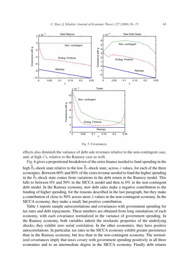
effects also diminish the variance of debt sale revenues relative to the non-contingent case,and, at high �’s, relative to the Ramsey case as well.

Fig. 6 gives a proportional breakdown of the extra finance needed to fund spending in the

high �3-shock state relative to the low �1-shock state, across � values, for each of the threeeconomies. Between 60% and 80% of the extra revenue needed to fund the higher spendingin the �3-shock state comes from variations in the debt return in the Ramsey model. Thisfalls to between 0% and 50% in the SICCA model and then to 0% in the non-contingentdebt model. In the Ramsey economy, new debt sales make a negative contribution to thefunding of higher spending, for the reasons described in the last paragraph, but they makea contribution of close to 50% across most �-values in the non-contingent economy. In theSICCA economy, they make a small, but positive contribution.

Table 1 reports sample autocorrelations and covariances with government spending fortax rates and debt repayments. These numbers are obtained from long simulations of eacheconomy, with each covariance normalized in the variance of government spending. Inthe Ramsey economy, both variables inherit the stochastic properties of the underlyingshocks; they exhibit zero serial correlation. In the other economies, they have positiveautocorrelations. In particular, tax rates in the SICCA economy exhibit greater persistencethan in the Ramsey economy, but less than in the non-contingent economy. The normal-ized covariances imply that taxes covary with government spending positively in all threeeconomies and to an intermediate degree in the SICCA economy. Finally debt returns


0 0.05 0.1 0.15 0.2 0.25 − 0.2

− 0.1

0

0.1

0.2

0.3

0.4

0.5

0.6

0.7

0.8

λ

Pro

port

ion

Return on Debt

Non−contingent

Endog. Frictions

Ramsey

0 0.05 0.1 0.15 0.2 0.25 − 0.2

− 0.1

0

0.1

0.2

0.3

0.4

0.5

λ

Pro

port

ion

New Debt Sales

Ramsey

Endog. Frictions

Non−contingent

0 0.05 0.1 0.15 0.2 0.250.3

0.35

0.4

0.45

0.5

0.55

0.6

0.65

λ

Pro

port

ion

Taxes

Non−contingent

Endog. Frictions

Ramsey

Fig. 6. Financing spending.

Table 1Summary statistics

Frictions Ramsey Non-contingent

�(�) 0.364 0.0d0 0.643�(b) 0.600 0.0d0 0.769Cov(�, g) 0.332 0.267 0.592Cov(b, g) −0.453 −0.694 −0.101

covary negatively with government spending in all economies, even in the non-contingentdebt economy. 15

6.4. Welfare comparisons

Lastly, we provide a welfare comparison between the SICCA economy and the benchmarkRamsey model. We calculate, for each initial �0, the reduction in household consumption

15 The latter result reflects the fact that at higher debt levels there is less government spending and larger salesof debt.


needed in all states and periods for the household to be indifferent between the Ramseyallocation eR(�0) and the optimal SICCA at �0. For our parameterization, this reductionaverages 0.053% of the household’s Ramsey consumption across �0 values, rising to apeak of 0.07% at the � boundaries. This small loss is consistent with the welfare findingsof AMSS, and indicates the capacity of tax smoothing across periods to substitute for taxsmoothing across states.

7. Conclusions

The empirical properties of tax rate and debt processes contrast with the implicationsof the Ramsey model and are suggestive of incomplete government insurance. This paperdevelops techniques for analyzing optimal fiscal policy under two frictions, private govern-ment information and limited government commitment. We find that these frictions implyendogenous debt value limits, a reduced smoothing of taxes across states, and enhancedpersistence in tax rates and debt levels. The government retains some ability to hedge againstfiscal shocks, so that the ensuing allocations and fiscal policies in our model lie somewherebetween those implied by the Ramsey model and a model with exogenously non-contingentdebt. This brings our model into line with evidence reported by Marcet and Scott [23].

Appendix A. Proofs

Proof of Lemma 4. Since, under xaut, st (hgt ) = 1 for all t, h

gt , households anticipate a full

default by the government after each history. Thus, after each ht , it is weakly optimal forthem to purchase no debt and their continuation problem reduces to a sequence of problemsof the form (10). When the government implements the autarkic menu xaut, households’op-timal choices are given by caut and laut. The government’s strategy implies choices that arebudget feasible for it and resource feasible for the economy. Since households, anticipatingfuture default, purchase no debt at a positive price, the government can not raise revenuefrom debt sales. It looses nothing from setting debt prices to zero. Its problem, after eachht , also reduces to a sequence of static problems. The government maximizes its payoffby defaulting on any outstanding debt, setting the transfer St to zero. Given that the gov-ernment must balance its budget, �aut(�) gives the optimal tax rate. The choices describedby (xaut(�), gaut(�)) are optimal for the government given a current shock realization of �.Consequently, the government has no incentive to lie and �g,aut satisfies the sequence ofoptimality conditions (8). It follows that (b0, �g,aut, �h,aut) is a sustainable equilibrium.

For any b0, the strategy �g,aut is always feasible for the government. If the governmentimplements (xaut, gaut) and reports �, the household will face a set of zero bond prices and,essentially, a static choice problem. Confronted with the tax rate �aut(�) and with s(�) = 1and S(�) = 0, it will be optimal for households to make the consumption and labor choicescaut(�) and laut(�). Thus, after any ht , by repeatedly implementing the menu xaut and beingtruthful, the government can guarantee itself the autarkic payoff. Thus, this payoff acts asa lower bound on the set of sustainable equilibrium payoffs. �


Proof of Proposition 5. (ONLY IF) Fix a sustainable equilibrium � = (�g, �h) at �0 withoutcome allocation e∞ = {ct , lt , gt }∞t=0 ∈ �. By the first condition of Definition 7, e∞ isa competitive allocation and, hence, satisfies Condition A of the proposition. By Condition1(b) of Definition 7, e∞ is part of a competitive equilibrium that entails no governmentlending. Therefore, for each t, �t , c−�

t (�t )[(1 − st (�

t ))bt (�t ) + St

(�t ))]

�0, where st (�t ),

bt (�t ), St

(�t)

are variables associated with the equilibrium. The household’s first orderconditions and budget constraint then imply (13).

Denote the reporting functions associated with �g by{ �t

}∞t=0. Note that the definition

of a sustainable equilibrium does not require them to be truthful, i.e. �t (ht (�g, �t−1), �)

need not equal �. Let { t }∞t=0 denote an arbitrary reporting policy. Suppose the govern-ment sought to obtain the allocation e∞( ) = {

ct ( t (�t )), lt (

t (�t )), gt ( t (�t ))

}∞t=0. It

could do this in the policy game by implementing the menu functions implied by �g , andaltering the reporting functions along the outcome path to:

�t (ht (�g, t−1(�t−1)), �t ) =

�t (ht (�g, t−1(�t−1)), t (�

t )). Equivalently, the government can obtain the allocatione∞( ) by making the reports that it would have made if the shock histories

{ t (�t )

}had

actually occurred. Since this is a feasible deviation in the policy game and the governmentchooses not to make such reports, it must be the case that the allocation e∞ gives a higherutility than e∞( ), and, hence, satisfies the incentive compatibility condition (14). After anyht , the government can always feasibly deviate to the policies associated with the autarkicequilibrium. Thus, the continuation of the outcome allocation must deliver a payoff abovethe autarkic one and (15) is satisfied.

(IF) Suppose an interior allocation e∞ = {ct , lt , gt }∞t=0 satisfies the conditions of theproposition, then a sustainable equilibrium at �0 can be constructed that supports it as an

outcome allocation. This is done as follows. Set, for all t, �t , �t (�t ) = 1 − c

�t (�t

)(T −lt (�

t))� , and

st (�t ) = 0. For t �1, set St (�

t ) = 0, and bt (�t ) so that c−�

t (�t )bt (�t ) = E�t

∑∞s=0 �sJ (ct+s

(�t+s), lt+s(�t+s)). For t = 0, choose S0(�

0) ∈ R+ and b0(�0) ∈ R+ to satisfy c

−�0 (�0)

(b0(�0)+S0(�

0))=E�0∑∞

s=0 �sJ (cs(�s), lt+s(�

s)), and �0=E[c−�0 (�0)(1−s0)b0(�

0)]. Set

qt so that the household’s Euler equations hold at the allocation. Set x∞ = {xt }∞t=0, withxt (�

t ) = {st (�t ), �t (�t ), St (�

t ), qt (�t )}.

We construct �g and �h history-by-history as follows. Let Hxt = {ht |ht =

{b0, xs(�

s−1),

gs(�s−1), �s

}t−1

s=0

}. Interpret Hx

t as the set of t-period public histories that are consis-

tent with the government implementing (x∞, g∞). Note that the occurrence of ht ∈Hx

t does not imply that the government has been truthful. If ht ∈ Hxt , set �g

t (ht ) to{xt (�

t−1), gt (�t−1), ∗}. and �h

t−1(ht ) to{ct−1(�

t−1), lt−1(�t−1), bt (�

t−1)}

. If ht /∈ Hxt ,

set �gt (ht ) to

{xaut, gaut, ∗} and �h

t−1(ht ) to the autarkic choices that solve (10).By construction, e∞ is the outcome allocation of �. Condition A of the proposition and

the proof of Proposition 1 then establishes that e∞, {bt }∞t=0 and x∞ form a competitive equi-librium with initial debt value �0. Thus, for all t, ht ∈ Hx

t , Conditions (1a) and (1c) of Def-inition 7 are satisfied. After all histories ht /∈ Hx

t , the definition of the autarkic equilibriumagain implies that Conditions (1a) and (1c) of Definition 7 are satisfied. Condition (1d) of


the definition is satisfied by construction. There is no borrowing in the autarkic equilibrium.The construction of the {bt }∞t=0 and (13) then implies that (1b) in the definition is satisfied.It remains to check Condition 2 of the definition. Since, after a history ht (�g, �t−1), anydeviation from (xt (�

t−1), gt (�t−1)) leads households to make the autarkic choices, when it

deviates from (xt (�t−1), gt (�

t−1)), the government can do no better than to choose the au-tarkic menu in the current period, and implement this in all future periods. This will delivera payoff of V aut to the government. By (15), this is below the payoff that the governmentobtains from continuing to implement the menus associated with the allocation and beingtruthful. Thus, the government will never deviate from the sequence (x∞, g∞). The gov-ernment can still deviate by implementing (x∞, g∞) and altering its reporting strategy. Any

allocation obtained by such a deviation is of the form:{c t , l

t , g

t

}∞t=0

, where, for each t, �t ,

c t (�

t ) = c�t (ht+1(�g, t (�t ))) = ct (

t (�t )), l t (�t ) = l�t (ht+1(�g, t (�t ))) = lt ( t (�t )),

g t (�t ) = g�

t (ht (�g, t−1(�t−1)), t (�t )) = gt (

t (�t )) and { t }∞t=0 is a reporting policy. By(14) such a deviation is not profitable for the government and Condition 2 of the definitionis verified. � is a sustainable equilibrium. �

We now turn to the task of characterizing a SICCA.

Lemma A.1. Suppose that e∞ = {ct , lt , gt }∞t=0 ∈ EIC(�0). Let e∞t+1|�t = {

cr

(�t , ·) ,

lr (�t , ·), gr(�

t , ·)}∞r=t+1denote the continuation allocation implied by e∞ after shock his-

tory �t . Let {�t }∞t=0 be a sequence of debt value functions consistent with e∞. Then, for allt, �t , e∞|�t ∈ EIC(�t+1(�

t )).

Proof. Since e∞ is a SICCA and {�t }∞t=0 is consistent with e∞, then for all �t , �t (�t )�E�t

[∑∞r=0 �rJ (ct+r , lt+r )]. Also e∞ satisfies the resource constraints after all histories. Hence,

for all t, �t , e∞|�t satisfies the competitive allocation requirements in Proposition 5. Addi-tionally, e∞ satisfies the no lending and sustainability constraints (13) and (15) after eachhistory. Furthermore, since P t(�t ) > 0, e∞ is incentive compatible only if each e∞|�t is.Hence, for all t, �t , e∞|�t ∈ EIC(�t+1(�

t )). �

Lemma A.2. A pair (v, �) is supported by a SICCA if and only if there exist functions{c, l, g, v′, �′}, with c : � → R+, l : � → R+, �′ : � → R+, v′ : � → R, such that:

v =∑�∈�

[W(c(�), l(�), g(�); �) + �v′(�)

]P(�), (45)

��∑�∈�

[J (c(�), l(�)) + ��′(�)

]P(�), (46)

∀�, l(�) − c(�) − g(�)�0, (47)

∀�, J (c(�), l(�)) + ��′(�)�0, (48)

∀(�, �), W(c(�), l(�), g(�); �) + �v′(�)�W(c(�), l(�), g(�); �) + �v′(�), (49)

68 C. Sleet, S. Yeltekin / Journal of Economic Theory 127 (2006) 36–73∑�∈�

[W(c(�), l(�), g(�); �) + �v′(�)]P(�)�V aut, (50)

∀�, (v′(�), �′(�)) ∈ W. (51)

Proof. (ONLY IF) Suppose (v, �) ∈ W , then there exists a SICCA, e∞ = {ct , lt , gt }∞t=0 ∈EIC(�), with v = V g(e∞). Set v′(�) = V g(e∞|�) and �′(�) = �1(�), where �1 is a con-sistent debt value, c = c0 and l = l0. Then, v = V g(e∞) = E

[W(c0(�), l0(�), g0(�); �)

+�V g(e∞|�)] = E

[W(c(�), l(�), g(�); �) + �v′(�)

], which confirms (45). Since �1 is

consistent, ��∑

�∈�[J (c0(�), l0(�)) + ��1(�)

]P(�), which confirms (46). (48), (49) and

(50) follow from the fact that e∞ satisfies (13), (14) and (15), respectively. By Lemma A.1,e∞|� ∈ EIC(�1(�)) and, so for each �, (V g(e∞|�), �1(�)) ∈ W . This confirms (51). (47)follows from resource feasibility of e∞ in period 0.

(IF) Suppose that for (v, �), there exists a four-tuple {c, l, g, v′, �′} satisfying the con-ditions in the lemma. Then, by (51), for each �, there exists a e∞

1 (�) = {ct , lt , gt }∞t=0 ∈EIC(�′(�)), with v′(�) = V g(e∞

1 (�)). Define e∞ = {c, l, g, e∞

1

}. It is straightforward to

check that this satisfies all the properties of a SICCA and has initial payoff and debt value(v, �). �

Let W (�) denote the set of {c, l, g, v′, �′} tuples satisfying conditions (46) to (51). Itfollows from Lemma A.2 that

V S(�) = sup{c,l,g,v′,�′}∈W (�)

∑�∈�

[W(c(�), l(�), g(�); �) + �v′(�)

]P(�). (52)

To prove Proposition 6, we first give a series of preliminary lemmas. These require achange of variables. 16 Given c : � → R+, l : � → [0, T ], and g : � → R+, let u(�) =c1−�(�), y(�) = (T − l(�))1−�, r(�) = g(�)1− and Y = {

(T − l)1−� : l ∈ [0, T ]}. We

recast problem (52) in terms of these utility variables:

sup{u,y,r,v′,�′}∈′

W (�)

∑�∈�

[F(u, y, r, �, �) + �v′(�)

]P(�) (53)

where F(u, y, r, �′, �) = u(�′)

1−� + y(�′)

1−� + � r(�′)

1− and ′W (�) equals all

{u, y, r, v′, �′} satis-

fying:

��∑�∈�

[u(�) +

(y(�) − Ty(�)

−�1−�

)+ ��′(�)

]P(�), (54)

∀�, T − y1

1−� (�) − u1

1−� (�) − r1

1− (�)�0, (55)

16 This change of variables is valid for � ∈ (0, 1) and � ∈ (0, 1) and �= 1. For �, � or equal to 1, analogousresults hold with u(�) = log c(�), y(�) = log(T − l(�)) and r(�) = log(g(�)). Related results also hold for thecase � = 0.


∀�, u(�) +(y(�) − Ty(�)

−�1−�

)+ ��′(�)�0, (56)

∀(�, �), F (u, y, r, �, �) + �v′(�)�F(u, y, r, �, �) + �v′(�), (57)∑�∈�

[F(u, y, r, �, �) + �v′(�)]P(�)�V aut, (58)

∀�, (v′(�), �′(�)) ∈ W, (59)

u(�) ∈ R+, y(�) ∈ Y, r(�) ∈ R+. (60)

The operator T can be re-expressed using utility variables. For (V , �) ∈ Q, � ∈ �(V , �) ≡{��0 : ′

V,�(�) �= �}, let

V ′(V , �)(�) = sup{u,y,r,�′,v′}∈′

V,�(�)

∑�∈�

[F(u, y, r, �, �) + �v′(�)]P(�). (61)

where ′V,�

(�) is defined to be all{u, y, r, v′, �′} that satisfy (54), (55), (56), (57), (60)

and

∀ �, v′(�) � V (�′(�)) (62)

�′(�) ∈ [0, �]. (63)

Also, let �′(V , �) = {� ∈ �(V , �) : V ′(V , �) (�) �V aut}. Then, T�(V , �) = sup �′(V , �),

while, for � ∈ �′(V , �), TV (V, �)(�) = V ′(V , �)(�).

Lemma A.3. T : Q → Q.

Proof. Fix (V , �) in Q. The convexity and compactness of the graph of ′V,�

implies that

′V,�

is continuous and that �(V , �) is convex and compact. The continuity of V ′(V , �) on

�(V , �) follows from the Theorem of the Maximum; the concavity of V ′(V , �) on �(V , �)

follows from the concavity of the objective and the convexity of the graph of ′V,�

. It follows

that �′(V , �) is an interval of the form [�′, �′] and TV (V, �) is concave and continuous.Since, the constraint set for problem (61) at a � ∈ �S relaxes that for the SICCA problem (53)(V (�)�V S(�) and �S ⊆ [0, �], so ′

W (�) ⊆ ′V,�

(�)), and tightens that governing an ar-

bitrary competitive allocation, V S(�)�TV (V, �)(�)�V R(�). Also, �S ⊆ �′(V , �) ⊆ �R .The latter implies that �′ = 0. It remains to check that TV (V, �)(�

′) = V aut. Suppose that

TV (V, �)(�′) > V aut. At each � from 0 to (V R)−1(V aut), there exists an optimal “static”

SICCA that solves:

sup(1 − �)−1∑�∈�

[F(u, y, r, �, �)

]P(�) subject to (55), (60) and (64)


��(1 − �)−1∑�∈�

[u(�) +

(y(�) − Ty(�)

−�1−�

)]P(�), (65)

∀�, u(�) +(y(�) − Ty(�)

−�1−�

)�0, (66)

∀(�, �), F (u, y, r, �, �)�F(u, y, r, �, �). (67)

At any � ∈ [0, �′], the payoff from this static allocation is less than TV (V, �)(�). Let

� = �′ + �, for � > 0 and small. Then it is possible to take a convex combination of

the solution to the optimal static SICCA problem at � and the solution at �′. Label thecorresponding convex combination of � and �′, ��. If the weight attached to the solution

at �′ is large enough, the convex combination of solutions will be feasible at ��. It willbe incentive compatible, deliver a payoff above autarky, and satisfy the implementabilityconstraint at ��. But since �� > �

′, the maximality of �

′is contradicted. �

Lemma A.4. For (V , �), (V ′, �′) ∈ Q with (V , �) � (V ′, �′) then T (V , �) � T (V ′, �′).

Proof. Follows directly from the fact that the constraint sets for the optimizations defined byT (V ′, �′)(�), � ∈ �(V ′, �′) are smaller than for the optimizations defined by T (V , �)(�).

�

Lemma A.5. Each term of the sequence {T n(V R, �R)} lies in Q and converges to a point

(V∞, �∞) ∈ Q. (V∞, �∞) is a fixed point of T .

Proof. It is easily verified that (V R, �R) ∈ Q. Thus, by Lemma A.3, each term of the

sequence is in Q. Moreover, the pair (V R, �R) is a fixed point of an operator that does

not incorporate the no lending, sustainability and incentive compatibility constraints. Thus,

T (V R, �R) (V R, �

R) and the sequence {T n(V R, �

R)} is a decreasing one. Let (Vn, �n) =

T n(V R, �R). Since it is decreasing and bounded below by 0, the sequence {�n}∞n=1 has a

limit, �∞. Since{�n

}∞n=1

is decreasing, for each � ∈ [0, �∞], {Vn(�)}∞n=1 is a well defined

sequence. It is decreasing and bounded below by V aut, and, hence, it converges to a limitV∞(�). Since V∞ is the pointwise limit of the decreasing sequence {Vn} and since each Vn

satisfies V S �Vn on �S , Vn �V R on [0, �∞] and is continuous and concave on [0, �∞],V∞ also satisfies these properties. Also, limn→∞ Vn(�∞)�V aut, so V∞(�∞)�V aut. IfV∞(�∞) > V aut, then for all n, Vn(�∞) > V aut, but then by continuity of the Vn functionsand the fact that limn→∞ �n = �∞, there exists an N such that for n > N , Vn(�n) > V aut,

a contradiction. Thus,{(

Vn, �n

)}∞n=1

converges to(V∞, �∞

)∈ Q. We now establish that(

V∞, �∞)

=(TV (V∞, �∞), T�(V∞, �∞)

).


Part 1:(V∞, �∞

)�(TV (V∞, �∞), T�(V∞, �∞)

). If � /∈ �∞, then � > �∞ and there

exists some N� such that � > �n, n > N�. By the monotonicity of T�, T�(V∞, �∞)�T�(Vn,

�n) = �n+1 for all n. Hence, � > T�(V∞, �∞) and T�(V∞, �∞)��∞. For � ∈ [0, T�(V∞,

�∞)],TV (V∞, �∞)(�) = sup{u,y,r,v′,�′}∈′V∞,�∞ (�)

∑�∈�

[F(u, y, r, �, �) + �v′(�)

]P(�)

� sup{u,y,r,v′,�′}∈′Vn,�n

(�)

∑�∈�

[F(u, y, r, �, �) + �v′(�)

]P(�) = TV (Vn, �n)(�) =

Vn+1(�). Taking the limit as n goes to infinity, we have, TV (V∞, �∞)(�)�V∞(�).

Part 2:(V∞, �∞

) (TV (V∞, �∞), T�(V∞, �∞)

). Let �∈�∞. Denote a solution to the

problem TV (Vn, �n)(�) by{un, yn, rn, v

′n, �

′n

}. Each

{un, yn, rn, v

′n, �

′n

} ∈ ′Vn,�n

(�) ⊆′

V R,�R (�). Since ′

V R,�R (�) is a compact set,

{un, yn, rn, v

′n, �

′n

}∞n=1 has a convergent sub-

sequence{unk

, ynk, rnk

, v′nk

, �′nk

}∞k=1

. Denote the limit{u∞, y∞, r∞, v′∞, �′∞

}. Since

�′nk

��nkeach k, �′∞ = limk→∞ �′

nk� limk→∞ �nk

= �∞ and V∞(�′∞(�)) is well definedfor each �. Additionally, V∞(�′∞(�)) = limn→∞ Vn(�

′∞(�)) = limn→∞ limk �n Vn(�′nk

(�))� limn→∞ limk �n Vnk(�′

nk(�))� limn→∞ limk �n v′

nk(�) = v′∞(�), where the second

equality comes from the continuity of Vn, and the first inequality uses the fact that k, and,hence, nk �n, and that the sequence of value functions is a decreasing one. The secondinequality uses Vnk

(�′nk

(�))�v′nk

(�). The other constraints that comprise ′V∞,�∞

(�) define

closed sets. Hence,{u∞, y∞, r∞, v′∞, �′∞

} ∈ ′V∞,�∞

(�), and TV (V∞, �∞)(�)�∑

�∈�[F(u∞, y∞, r∞, �, �) + �v′∞(�)

]P(�) = limk→∞

∑�∈�

[F(unk

, ynk, rnk

, �, �)

+ �v′nk

(�)](P (�)= limk→∞ Vnk

(�)=V∞(�). Moreover, if�∈�′(V∞, �∞)⊆�′(Vn, �n), then

V∞(�) = limn→∞ Vn(�)�V aut. Hence, for all � ∈ �′(V∞, �∞), TV (V∞, �∞)(�)�V∞(�)�V aut and T�(V∞, �∞)(�)��∞. �

Lemma A.6. For (V , �) ∈ Q and each � ∈T�(V , �), there exists a solution to problem(61) that satisfies, for all �, v′(�) = V (�′(�)).

Proof. Let �, �(�), �(�), �(�), �(�) be Lagrange multipliers on, respectively, the imple-mentability constraint (54), the constraint on debt repayment values in state � (56), con-straint (62), and the upper and lower boundary constraints on �′(�) (63). Let �V (�) denotethe set of sub-differentials of V at �.

The first order condition for �′(�) is 0 ∈ �P(�) + �(�) + �(�)�V (�′(�)) + �(�) − �(�).

Suppose there is a solution such that �P(�) + �(�) > 0 and v′(�) < V (�′(�)). Then�(�) = 0, �(�) > 0 and �′(�) = �. But at �′(�) = �, V aut �v′(�) < V (�′(�)) =V aut, a contradiction. Suppose then that there is a solution with �P(�) + �(�) = 0, andv′(�) < V (�′(�)). Consider raising �′(�) slightly. This relaxes the constraints (54) and(56) in state �, and if v′(�) is still feasible it does not reduce the government’s pay-off. Raise �′(�) until either (i) v′(�) = V (�′(�)), or (ii) �′(�) = �. In the first case,the required condition holds immediately. In the second, it follows from V aut �v′(�)�V (�) = V aut. �


Lemma A.7. Each (V∞(�), �), � ∈ �∞ ≡ [0, �∞] is supported by a SICCA.

Proof. Let u∞ : �∞ × � → R+, y∞ : �∞ × � → R+, r∞ : �∞ × � → R+, �′∞ :�∞ × � → �∞, v′∞ : �∞ × � → [

V aut, V R(0)]

denote policy functions from the prob-lem TV (V∞, �∞) that satisfy v′∞(�) = V∞(�′∞(�)). Define the resource policy functions:

c∞ = u1/1−�∞ , l∞ = T − y

1/1−�∞ and g∞ = r

1/1−∞ . Given an initial �0 ∈ �∞, construct

an allocation recursively by iterating on the equations: lt (�t ) = l∞(�t (�

t−1), �t ), ct (�t ) =

c∞(�t (�

t−1), �t

), gt (�

t ) = g∞(�t (�

t−1), �t

)and �t+1(�

t ) = �∞(�t (�t−1), �t ). After

each �t , the functions {ct , lt , gt }∞t=0 satisfy the resource constraint and the recursive imple-mentability constraint (46). Since �t+1(�

t ) ∈ �∞ for all t, �t , limt→∞ �tE0[�t+1(�t )] = 0

and the allocation {ct , lt , gt }∞t=0 is competitive. Similarly, the constraint (46), the bounded-ness of the �∞ function and the recursive no lending condition (48) imply that, for all t, �t ,E�t

[∑∞s=t �s−t J (cs, ls)

]�0 so that the allocation satisfies the no lending conditions (13).

Repeatedly using TV (V∞, �∞) and the constructed allocation yields V∞(�0)=E[∑T

t=0 �tW(ct , lt , gt ; �t )]+E

[�T +1V∞ (�T +1)

]. Taking the limit as T goes to infinity

and using V R(0)�V∞(�)�V aut implies that V∞(�0) gives the payoff from the allocation.Similarly, V∞(�t (�

t )) gives the continuation payoff from the allocation after the history�t . Since, for all �t , �t (�

t ) ∈ �∞, then for all �t , V∞(�t (�

t ))

�V aut, and the allocationsatisfies the sustainability constraints. It also satisfies a sequence of recursive incentivecompatibility constraints. ∀t, �t , � :

W(ct (�t ), lt (�

t ), gt (�t ); �t ) + �V∞(�t+1(�

t ))

�W(ct (�t−1, �), lt (�

t−1, �), gt (�t−1, �); �t ) + �V∞(�t+1(�

t−1, �)).

By an argument ofAtkeson and Lucas [6], these recursive incentive compatibility constraintsand the boundedness of V∞ imply that the allocation is incentive compatible. Thus, theallocation is a SICCA. �

Proof of Proposition 6. Part 2: (Sketch). The first part of the proof is a standard dynamic

programming argument. It proceeds by showing that if V S(�) < TV (V S, �S)(�), � ∈ �S ,

then there exists a SICCA consistent with � that delivers a payoff in excess of V S(�), a

contradiction. Conversely, if V S(�) > TV (V S, �S)(�), then there exists a feasible choice

for problem (61) that delivers a payoff in excess of TV (V S, �S)(�), again a contradiction.

So V S(�) = TV (V S, �S)(�), � ∈ �S . It then follows from the definition of T� that �

S =T�(V

S, �S).

Part 3: Using the monotonicity of T and the result from Part 2, (V S, �S) = T (V S, �

S)

T (V R, �R) ((V R, �

R). Hence, iterating on these conditions: (V S, �

S) (V∞, �∞) =

limn→∞ T n(V R, �R). But since each (V∞(�), �), � ∈ �∞ is supported by a SICCA,

(V S, �S) � (V∞, �∞). Hence, combining inequalities, (V S, �

S) = (V∞, �∞).

Part 1: Follows from the fact that (V S, �S) = (V∞, �∞) ∈ Q. �


References

[1] D.Abreu, D. Pearce, E. Stacchetti, Towards a theory of discounted repeated games with imperfect monitoring,Econometrica 58 (1990) 1041–1064.

[2] R. Aiyagari, A. Marcet, T. Sargent, J. Seppälä, Optimal taxation without state contingent debt, J. Polit.Economy 110 (2002) 1220–1254.

[3] F. Alvarez, U. Jermann, Efficiency, equilibrium and asset pricing with risk of default, Econometrica 68 (4)(2002) 775–797.

[4] G.-M. Angeletos, Fiscal policy with non-contingent debt and the optimal maturity structure, Quart. J. Econ.117 (3) (2002) 1105–1131.

[5] S. Athey, A. Atkeson, P. Kehoe, The optimal degree of monetary policy discretion, FRB of Minneapolis W.P.626, 2003.

[6] A. Atkeson, R. Lucas, On efficient distribution with private information, Rev. Econ. Stud. 59 (1992)427–453.

[7] R. Barro, Reputation in a monetary model with incomplete reputation. J. Monet. Econ. 17 (1986) 3–20.[8] D. Bizer, S. Durlauf, Testing the positive theory of government finance, J. Monet. Econ. 26 (1990) 123–141.[9] H. Bohn, Tax smoothing with financial instruments, Amer. Econ. Rev. 80 (1990) 1217–1230.

[10] G. Calvo, P. Guidotti, Indexation and maturity of government bonds: an exploratory model, in: R. Dornbusch,M. Draghio (Eds.), Public Debt Management: Theory and History, Cambridge University Press, Cambridge,1990.

[11] M. Canzoneri, Monetary policy games and the role of private information, Amer. Econ. Rev. 75 (1985)1056–1070.

[12] R. Chang, Credible monetary policy in a infinite horizon model: recursive approaches, J. Econ. Theory 81(1998) 431–481.

[13] V. Chari, L. Christiano, P. Kehoe, Optimal fiscal policy in a business cycle model, J. Polit. Economy 102(1994) 617–652.

[14] V. Chari, P. Kehoe, Sustainable plans, J. Polit. Economy 98 (1990) 783–802.[15] V. Chari, P. Kehoe, Sustainable plans and mutual default, Rev. Econ. Stud. 60 (1993a) 175–195.[16] V. Chari, P. Kehoe, Sustainable plans and debt, J. Econ. Theory 60 (1993b) 175–195.[17] V. Chari, P. Kehoe, Optimal fiscal and monetary policy, in: J. Taylor, M. Woodford (Eds.), Handbook of

Macroeconomics, North Holland, Amsterdam, 1999.[18] A. Cuckierman, A. Meltzer, A theory of ambiguity, credibility and inflation under discretion and asymmetric

information, Econometrica 54 (1986) 1099–1128.[19] J. Fernández-Villaverde, A. Tsyvinkski, Optimal fiscal policy in a business cycle model without commitment,

Unpublished paper, University of Pennsylvania, 2002.[20] C. Huang, K. Lin, Deficits, government expenditures and tax smoothing in the United States: 1929–1988,

J. Monet. Econ. 31 (1993) 317–339.[21] G. Kingston, Efficient timing of taxes, J. Public Econ. 24 (1987) 271–280.[22] R. Lucas, N. Stokey, Optimal fiscal and monetary policy in an economy without capital, J. Monet. Econ. 12

(1983) 55–93.[23] A. Marcet, A. Scott, Debt and deficit fluctuations and the structure of bond markets, Unpublished paper, UPF,

2001.[24] G.M. Milesi-Ferretti, Good, bad or ugly?, On the effects of fiscal rules with creative accounting, J. Public

Econ. 88 (2004) 377–394.[25] A. Missale, Public Debt Management, Oxford University Press, Oxford, 1999.[26] C. Phelan, E. Stacchetti, Sequential equilibria in a Ramsey model, Econometrica 69 (2001) 1491–1518.[27] A. Scott, Does tax smoothing imply smooth taxes?, CEPR WP 2172, 1999.[28] C. Sleet, On credible monetary policy and private government information, J. Econ. Theory 99 (2001)

338–376.[29] C. Sleet, Optimal taxation with private government information, Rev. Econ. Stud., 2003, forthcoming.[30] C. Sleet, S. Yeltekin, Optimal taxation with endogenously incomplete debt markets: technical appendix,

Mimeo, University of Iowa and Northwestern University, 2004.[31] X. Zhu, Optimal fiscal policy in a stochastic growth model, J. Econ. Theory 58 (1992) 189–250.