Newton Polytopes of Cluster Variables
by
Adam Michael Kalman
A dissertation submitted in partial satisfaction of the
requirements for the degree of
Doctor of Philosophy
in
Mathematics
in the
Graduate Division
of the
University of California, Berkeley
Committee in charge:
Associate Professor Lauren K. Williams, ChairProfessor Bernd Sturmfels
Professor Alistair J. Sinclair
Fall 2014

Newton Polytopes of Cluster Variables
Copyright 2014
by
Adam Michael Kalman

1
Abstract
Newton Polytopes of Cluster Variables
by
Adam Michael Kalman
Doctor of Philosophy in Mathematics
University of California, Berkeley
Associate Professor Lauren K. Williams, Chair
We study Newton polytopes of cluster variables in type An cluster algebras, whose cluster
and coefficient variables are indexed by the diagonals and boundary segments of a polygon.
Our main results include an explicit description of the affine hull and facets of the Newton
polytope of the Laurent expansion of any cluster variable, with respect to any cluster. In
particular, we show that every Laurent monomial in a Laurent expansion of a type A cluster
variable corresponds to a vertex of the Newton polytope. We also describe the face lattice
of each Newton polytope via an isomorphism with the lattice of elementary subgraphs of
the associated snake graph. Other results include a geometric interpretation of the proper
Laurent property in type A based on Newton polytopes, and a proof that the Newton
polytope of a type A cluster variable has no relative interior lattice points. We also consider
extensions of these ideas, results, and methods to other cluster algebras.

i
To Isaac and Jonah
ii
Contents
Contents ii
1 Introduction 11.1 Overview . . . . . . . . . . . . . . . . . . . . . . . . . . . . . . . . . . . . . . 11.2 The Cluster Algebra Associated to a Quiver . . . . . . . . . . . . . . . . . . 31.3 Cluster Expansions from Matchings . . . . . . . . . . . . . . . . . . . . . . . 7
2 Newton Polytopes of Cluster Variables of Type A 102.1 Affine Hull, Facets, and Face Lattice Results . . . . . . . . . . . . . . . . . . 102.2 Proofs and Minor Results . . . . . . . . . . . . . . . . . . . . . . . . . . . . 13
3 Other Results and Conjectures 333.1 Remarks for Type A . . . . . . . . . . . . . . . . . . . . . . . . . . . . . . . 333.2 Proper Laurent Property and No Interior Lattice Points for Type A . . . . . 343.3 Remarks and Conjectures for Other Cluster Algebras . . . . . . . . . . . . . 38
4 Code and Visualizations 404.1 Code and Output . . . . . . . . . . . . . . . . . . . . . . . . . . . . . . . . . 40
Bibliography 47

iii
Acknowledgments
I would first like to thank my advisor, Lauren Williams, for her unwavering guidance and
support, and for introducing me to the study of cluster algebras. I feel privileged to have
had the opportunity to work with such a talented mathematician and extraordinary person,
and I could never have made it to this point without her.
I would also like to thank the other faculty and staff of the UC Berkeley Mathematics
Department, especially Mark Haiman, Bernd Sturmfels, and Paul Vojta, for teaching me
lots of wonderful mathematics over these last few years and for taking time to serve on my
committees.
Special thanks go to Gregg Musiker, Dylan Thurston, and Jim Propp for helpful advice
and enlightening conversations.
Over the past few years, I have had the privilege of meeting and working with many
colleagues and collaborators who have generously shared their time and ideas, including
Christian Hilaire, Steven Karp, Jose Rodriguez, and the dozens of other truly amazing
graduate students I met along the way.
Finally, I would like to thank my family. Anna, Isaac, and Jonah, you are my inspiration
and my strongest support. It’s all for you.
1
Chapter 1
Introduction
1.1 Overview
Cluster algebras, introduced by Fomin and Zelevinsky in the early 2000’s [9, 10, 11], are a
class of commutative rings equipped with a distinguished set of generators (cluster variables)
that are grouped into sets of constant cardinality n (the clusters). A cluster algebra may be
defined from an initial cluster (x1, ..., xm) and a quiver, which contains combinatorial data
for the process of mutation, in which new clusters and quivers are created recursively from
old ones. There may also be coefficients involved in the construction. The cluster algebra is
the algebra generated by all cluster variables, after mutation is repeated ad infinitum.
The original motivation for cluster algebras was to create a combinatorial framework for
studying total positivity and dual canonical bases in semisimple Lie groups. Since then,
cluster structures have been studied in various areas of mathematics.
Perhaps the most fundamental example of a cluster algebra is the cluster algebra associ-
ated with triangulations of a polygon. Cluster algebras of finite type (i.e. those with finitely
many cluster variables) are classified by Dynkin diagrams, and the cluster algebras coming
from triangulations of a polygon are precisely those of type A. In this model, diagonals
correspond to cluster variables, triangulations (i.e. maximal collections of non-intersecting
diagonals) correspond to clusters, boundary segments correspond to coefficient variables,
and mutation corresponds to a local move called a flip of the triangulation, in which one
diagonal is replaced with another one.
A consequence of the definition of cluster algebra is that every cluster variable is a
rational function in the initial cluster variables, but more strongly, the remarkable Laurent
Phenomenon [9] states that every cluster variable is in fact a Laurent polynomial in those
variables.
In the last ten years, much work has been done on Laurent expansion formulas for cluster
CHAPTER 1. INTRODUCTION 2
algebras. Carroll and Price (in unpublished results [2]) were the first to discover formulas
for Laurent expansions of cluster variables in the case of a triangulated polygon, writing one
formula in terms of paths and another in terms of perfect matchings of so-called snake graphs
[19]. Their formula was subsequently rediscovered and generalized in a series of works [20],
[21], [22], [16], [18], with [18] providing Laurent expansions of cluster variables associated to
cluster algebras from arbitrary surfaces.
In this thesis, we study the Newton polytope of the Laurent expansion of a cluster
variable in a type A cluster algebra with respect to an arbitrary cluster. The study of
Newton polytopes of Laurent expansions of cluster variables was initiated by Sherman and
Zelevinsky in their study of rank 2 cluster algebras, in which it was shown that the Newton
polygon of any cluster variable in a rank 2 cluster algebra of finite or affine type is a triangle
[23]. We will extend these results in type A by considering cluster algebras of arbitrary rank.
One motivation for this study is that the cluster algebra of type An is isomorphic to the
coordinate ring of the affine cone over the Grassmannian Gr(2, n). From this perspective,
exchange relations in the cluster algebra correspond to three-term Plucker relations, and
Laurent expansions of cluster variables give expressions for arbitrary Plucker coordinates in
terms of a fixed set of algebraically independent Plucker coordinates. Thus the results in this
paper can be interpreted as results about the Grassmannian. For example, a facet description
of the Newton polytope can be interpreted in terms of constraints on Plucker coordinates.
Another motivation for the study of these Newton polytopes is that understanding Newton
polytopes of cluster variables has been useful for understanding bases of cluster algebras [3],
[23].
In the remainder of this chapter, we review the definition of a cluster algebra associated
to a quiver, as well as the relevant formula for Laurent expansion of a cluster variable in
terms of perfect matchings. Our main results in chapter 2 are explicit descriptions of the
affine hull and facets of the Newton polytope of a Laurent expansion of any cluster variable
of type An, as well as a description of the face lattice of such a polytope via an isomorphism
with the lattice of elementary subgraphs of the associated snake graph. Our affine hull and
facet description can be read off the triangulation directly. We also show that every Laurent
monomial in a Laurent expansion of a type A cluster variable corresponds to a vertex of the
Newton polytope. In chapter 3, we present other results for type A, including a geometric
interpretation of the proper Laurent property based on Newton polytopes, and a proof that
the Newton polytope of a type A cluster variable contains no relative interior lattice points.
We also consider extensions of these ideas, results, and methods to other cluster algebras.
Chapter 4 contains computer code written for the purpose of making computations with
cluster variables and generating conjectures, such as the ones that became the theorems and
propositions of chapters 2 and 3.
CHAPTER 1. INTRODUCTION 3
1.2 The Cluster Algebra Associated to a Quiver
A quiver is a directed graph. It consists of a set of vertices connected by arrows (oriented
edges), where there may be multiple arrows between pairs of vertices. In this section, we
will review the construction of a cluster algebra from a quiver with no 1-cycles or 2-cycles.
Note that a cluster algebra can be defined in much more generality than this, but this will
suffice for our purposes.
First we will define clusters and seeds. Let m and n be positive integers, with m ≥ n. Let
F be the ambient field of rational functions in n independent variables over Q(xn+1, . . . , xm).
Define the (extended) cluster as x = (x1, . . . , xm), a free generating set for F . We will call
{x1, . . . , xn} cluster variables, and {xn+1, . . . , xm} coefficient variables or frozen variables.
Let Q be a quiver whose vertices are labeled {1, . . . ,m}, where vertices {1, . . . , n} are called
mutable, and {n+ 1, . . . ,m} are called frozen. The pair (x, Q) is called a seed.
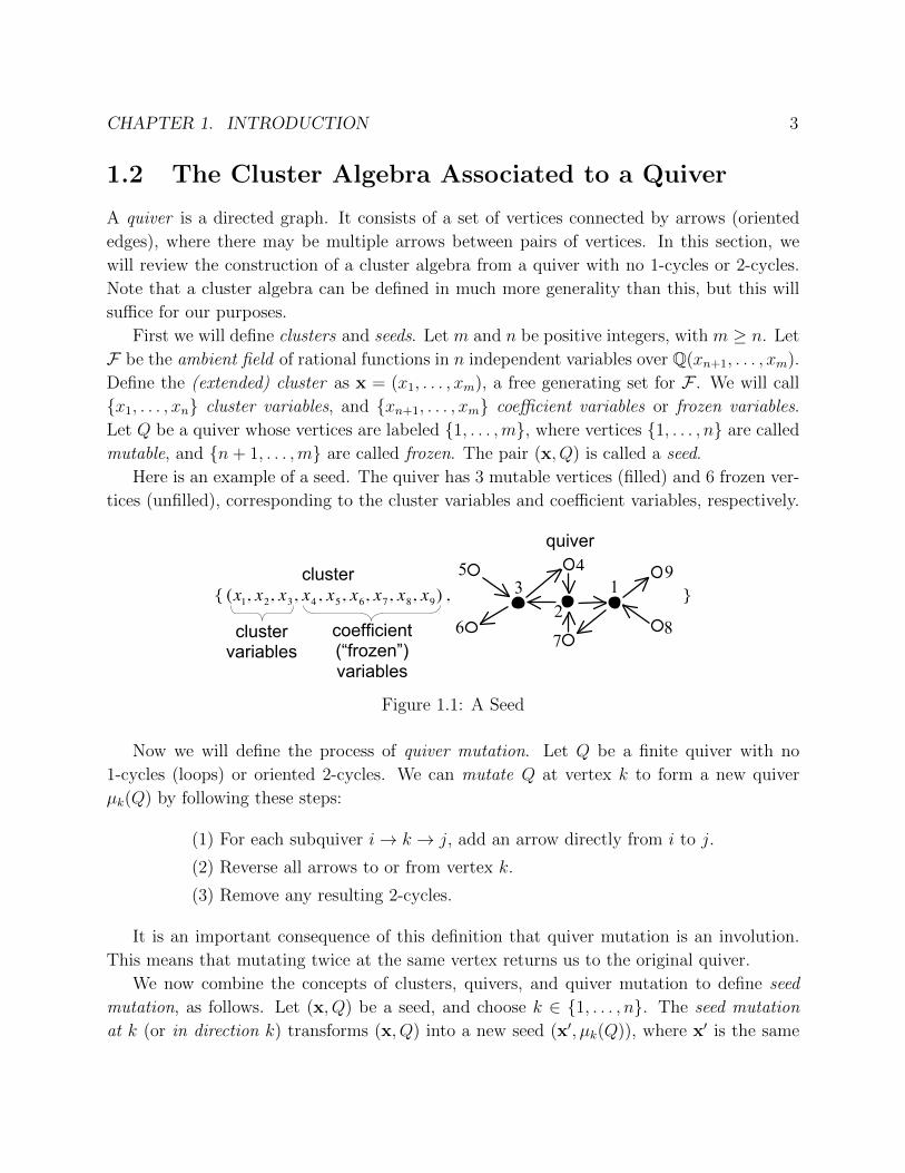
Here is an example of a seed. The quiver has 3 mutable vertices (filled) and 6 frozen ver-
tices (unfilled), corresponding to the cluster variables and coefficient variables, respectively.
!!!!!!!
€
{ (x1, x2, x3, x4, x5, x6, x7, x8, x9) , } !
quiver
cluster
cluster variables
coefficient (“frozen”) variables
1 2
3 4 5
7 8
9
6
Figure 1.1: A Seed
Now we will define the process of quiver mutation. Let Q be a finite quiver with no
1-cycles (loops) or oriented 2-cycles. We can mutate Q at vertex k to form a new quiver
µk(Q) by following these steps:
(1) For each subquiver i→ k → j, add an arrow directly from i to j.
(2) Reverse all arrows to or from vertex k.
(3) Remove any resulting 2-cycles.
It is an important consequence of this definition that quiver mutation is an involution.
This means that mutating twice at the same vertex returns us to the original quiver.
We now combine the concepts of clusters, quivers, and quiver mutation to define seed
mutation, as follows. Let (x, Q) be a seed, and choose k ∈ {1, . . . , n}. The seed mutation
at k (or in direction k) transforms (x, Q) into a new seed (x′, µk(Q)), where x′ is the same

CHAPTER 1. INTRODUCTION 4
tuple as x, except that the kth entry, x′k, is determined by the quiver Q via the following
exchange relation:
x′k xk =∏i→k
xi +∏k→j
xj .
At this point it is worth noting a few things. First, seed mutation encompasses quiver
mutation, so we may overload the notation slightly and also denote it as µk. Moreover, seed
mutation is again an involution. It is also worth mentioning that there is a way to encode
the combinatorics of quivers and mutation in terms of matrices and a process called matrix
mutation. Finally, note that arrows between two frozen vertices of a quiver are not involved
in seed mutation, so they may be omitted from the quiver.
Since we may mutate a seed in n different directions, and mutation is an involution, we
may keep track of all possible seeds by assigning a seed to each vertex of an n-regular tree.
In this tree, the n undirected edges at each vertex are labeled uniquely from 1 to n, and
the seeds assigned to the endpoints of an edge labeled k are obtained from each other by
mutation at k. Note that the tree is uniquely determined by one of its seeds.
We will illustrate seed mutation with Figure 1.2, featuring part of the 3-regular tree that
results from mutating the seed from Figure 1.1.
To make sense of this diagram, we may look at the changes from the original seed (in the
center) to the seed on the lower right, created by mutation in direction 3. If we examine vertex
3 of the original quiver, we see it has arrows labeled 2 and 5 pointing in, and arrows labeled
4 and 6 pointing out. This gives the exchange relation x3x′3 = x2x5 + x4x6. Replacing x3
with x′3 = x2x5+x4x6x3
gives the mutated cluster on the lower right. Now the quiver is mutated
by first adding arrows from vertex 2 to vertex 6 (shown), vertex 5 to vertex 4 (omitted since
it is between frozen vertices), vertex 5 to vertex 6 (similarly omitted), and vertex 2 to vertex
4 (creating a 2-cycle), then reversing the four arrows incident to vertex 3, and then canceling
the 2-cycle between vertices 2 and 4.

CHAPTER 1. INTRODUCTION 5
!!!!!!!!!
µ 3
€
{ (x1,x1x3 + x4x7
x2, x3, ..., x9), }
!
1 2
3 4 5
7 8
9
6
€
{ (x1, x2, x3, ..., x9), }!
€
{ ( x2x8 + x7x9x1
, x2, x3, ..., x9), } !
€
{ (x1, x2,x2x5 + x4x6
x3, ..., x9), }!
1 2
3 4 5
7 8
9
6
1 2
3 4 5
7 8
9
6
1 2
3 4 5
7 8
9
6
µ 2
µ 1
µ 1 µ 3
µ 2 µ 1
µ 2 µ 3
Figure 1.2
With these structures and procedures defined, we are finally ready to define a cluster
algebra. If we take the union of all the clusters in all the seeds on our n-regular tree, we
obtain a list of all possible cluster variables. The cluster algebra A(x, Q) is the subalgebra
of the ambient field F generated by all cluster variables.
A quick examination of the exchange relations makes it clear that a cluster variable
must be a rational function in the variables of any cluster. In fact much more is true: each
cluster variable is in fact a Laurent polynomial in those variables. This so-called Laurent
Phenomenon (Theorem 3.1 in [9]) is the most important theorem in the study of cluster
algebras.
Theorem 1.2.1 (Laurent Phenomenon). Every element of the cluster algebra A(x, Q) is a
Laurent polynomial in the cluster variables (x1, . . . , xn).
Another surprising result is that a priori, the set of seeds is infinite, but in many cases,
there are only a finite number of distinct cluster variables or distinct quivers. In fact the

CHAPTER 1. INTRODUCTION 6
classification of finite type cluster algebras (those with a finite number of seeds) is identical
to the well-known Cartan-Killing classification of simple Lie algebras. Specifically, a cluster
algebra is of finite type if and only if it has a seed whose quiver is an orientation of a finite
type Dynkin diagram.
Next, we will consider the finite type cluster algebra known as type An. This cluster
algebra can be modeled using triangulations of an (n+ 3)-gon. In this model, each diagonal
corresponds to a cluster variable, and each triangulation (i.e. maximal collection of non-
intersecting diagonals) corresponds to a cluster. The boundary segments of the polygon
correspond to coefficient (frozen) variables. Mutation at k is modeled by a local move
called a flip of the diagonal labeled with xk, in which that diagonal is removed to form a
quadrilateral, and then replaced with the other diagonal of that quadrilateral. The label on
this new diagonal is given by a Ptolemy relation which states that the product of the labels
of the old and new diagonals equals the sum of products of opposite sides of their common
quadrilateral. Here is an example that models the mutation in direction 3 from the example
in Figure 1.2. The reader is encouraged to examine the correspondence between the two
representations.
!!!!!!!!!
€
µ1
!
€
µ 2
!
€
µ 3
!€
x1!
€
x2!
€
x3!
€
x4!
€
x5!
€
x6!
€
x7!€
x8!
€
x9!
€
x2!
€
x4!
€
x5!
€
x6!
€
x7!€
x8!
€
x9!
€
x1!
€
x2x5 + x4x6x3
!
€
µ 2
!
€
µ1
!
Correspondences: {cluster variables} ↔ {diagonals} {clusters} ↔ {triangulations} {frozen variables} ↔ {boundary segments} {mutations} ↔ {diagonal flips}

CHAPTER 1. INTRODUCTION 7
For more details and a more general construction of cluster algebras from surfaces, see
[8]. The next section will detail an extraordinary formula for Laurent expansions of these
type A cluster variables.
1.3 Cluster Expansions from Matchings
The cluster algebra we are considering here is constructed from a triangulation T of an
(n+ 3)-gon as follows. Let τ1, τ2, . . . , τn be the n diagonals of T , and let τn+1, τn+2, . . . , τ2n+3
be the n+ 3 boundary segments.
The quiver QT is defined as follows: place a frozen vertex at the midpoint of each bound-
ary segment of the polygon, and place a mutable vertex at the midpoint of each diagonal.
These midpoint vertices form the vertices of QT . Label these vertices according to the label-
ing of the polygon. To form the arrows of QT , go to each triangle of T and inscribe a new
triangle connecting the midpoint vertices, orienting the arrows clockwise within this new
triangle. For example, here is a triangulation T of a hexagon, along with the correspond-
ing quiver QT , that forms the same example as in the previous section. The diagonals and
boundary segments of T are shown as thin solid lines. Mutable vertices of the quiver are
indicated by filled-in circles, frozen vertices are indicated by unfilled circles, and the arrows
of the quiver are dashed lines. QT =
1 2 3
4
5
7
8
9
6
Let A(QT ) be the cluster algebra with initial cluster variables (x1, ..., xn), coefficient
variables (xn+1, ..., x2n+3), and initial quiver QT . Each cluster variable in A(QT ) corresponds
to a diagonal. Let xγ be the cluster variable corresponding to the diagonal γ.
The cluster expansion of xγ with respect to T , or the T -expansion of xγ, means the Laurent
polynomial (equal to xγ) in the variables which each correspond to a diagonal or boundary
segment of T . The formula for the T -expansion of xγ in [16] for the cluster variables is given
in terms of perfect matchings of a graph GT,γ that is constructed using recursive gluing of
tiles. We now recount the construction of this graph GT,γ, as described in [16] and [17].

CHAPTER 1. INTRODUCTION 8
Let γ be a diagonal which is not in T . Choose an orientation on γ, and let the points of
intersection of γ and T , in order, be p0, p1, . . . , pd+1. Let τi1 , τi2 , . . . , τid be the diagonals of
T that are crossed by γ, in order.
For k from 0 to d, let γk denote the segment of the path γ from pk to pk+1. Note that
each γk lies in exactly one triangle in T , and for 1 ≤ k ≤ d− 1, the sides of this triangle are
τik , τik+1, and a third edge denoted by τ[γk].
A tile Sk is a 4-vertex graph consisting of a square along with one of its diagonals. Any
diagonal τk ∈ T is the diagonal of a unique quadrilateral Qτk in T whose sides we will call
τa, τb, τc, τd. Associate to this quadrilateral a tile Sk by assigning weights to the diagonal
and sides of Sk in such a way that there is a homeomorphism Qτk → Sk which maps the
diagonal labeled τi to the edge with weight xi, for i = a, b, c, d, k.
For each tile Si1 , Si2 , . . . , Sid , we choose a planar embedding in the following way: For
Si1 , the homeomorphism Qτi1→ Si1 must be orientation-preserving, and the vertex of Si1
which corresponds to p0 is placed in the southwest corner. Then, for 2 ≤ k ≤ d, choose a
planar embedding for Sik which has the opposite orientation of the previous tile Sik−1, and
orient the tile Sik so that the diagonal goes from northwest to southeast.
We then create the graph GT,γ by gluing together tiles Si1 , Si2 , . . . , Sid , in order, attaching
Sik+1to Sik along the edge on each tile that is labeled x[γk]. Note that the edge weighted
x[γk] is either the northern or the eastern edge of the tile Sik , and hence GT,γ is constructed
from the bottom left (the first tile) to the upper right (the last tile).
Definition 1.3.1. The snake graph GT,γ is the graph obtained from GT,γ after the diagonal
is removed from each tile.
See Figure 1.3 for an example of a triangulation T (along with distinguished diagonal γ)
and the corresponding snake graph.
T =
C
B
A
H
G
2
13
1
7 8
D
E
F
3 4
5 6
9
10
11 12
γ I
14
15
GT,γ =
c
b
a h
g
2
13
1
7 8
d
e f 3
4 5 6 9
10 11
12 5 4
3
a’
a”
b’ e’
Figure 1.3: An Example

CHAPTER 1. INTRODUCTION 9
Definition 1.3.2. A perfect matching of a graph is a subset of the edges so that each vertex
is covered exactly once. The weight w(M) of a perfect matching M is the product of the
weights of all edges in M .
With this setup, Laurent expansions of cluster variables can be expressed in terms of
perfect matchings as follows (see [16]).
Proposition 1.3.3. With the above notation,
xγ =∑M
w(M)
xi1xi2 . . . xid,
where the sum is over all perfect matchings M of GT,γ.

10
Chapter 2
Newton Polytopes of Cluster
Variables of Type A
An extended abstract version of this chapter was published in a proceedings volume of
DMTCS (Discrete Mathematics and Theoretical Computer Science).
2.1 Affine Hull, Facets, and Face Lattice Results
Before we can state our main results, we need a few more definitions and some new notation.
Definition 2.1.1. The Newton polytope of a Laurent polynomial is the convex hull of all
the exponent vectors of the monomials, i.e. the convex hull of all points (c1, c2, ...) such that
the monomial xc11 xc22 ... appears with a nonzero coefficient in the Laurent polynomial.
For ease of notation, we may sometimes say a diagonal or boundary segment of the
polygon is labeled k rather than τk.
Notation 2.1.2.
• Let D(γ) denote the set of diagonals of the triangulation that γ crosses, i.e. {τi1 , τi2 , . . . , τid}.
• Let T ′ be the subset of T that includes all vertices incident to a diagonal in γ ∪D(γ),
and all diagonals and boundary segments connecting these vertices to each other.
• For any point w ∈ T , let diagonals(w) := {e ∈ (γ∪D(γ)) : e 3 w}, the set of diagonals
in γ ∪D(γ) incident to w.
• Let the set of distinct labels of edges incident to a vertex v ∈ GT,γ be Ev. If V is a
collection of vertices, let EV :=⋃w∈V Ew

CHAPTER 2. NEWTON POLYTOPES OF CLUSTER VARIABLES OF TYPE A 11
• Let N(T, γ) be the Newton polytope (in R2n+3) of the T -expansion of the cluster variable
xγ.
• Let P (GT,γ) be the polytope in R2n+3 that is the convex hull of the characteristic vectors
of all perfect matchings of GT,γ.
Remark 2.1.3. By Proposition 1.3.3, the two polytopes N(T, γ) and P (GT,γ) are isomorphic,
differing only by a translation by the vector 1D(γ) (i.e. the vector whose ith coordinate is 1
if i ∈ D(γ), 0 otherwise). So P (GT,γ) can be thought of as the “Newton polytope of the
numerator” of the cluster variable corresponding to γ.
Definition 2.1.4. Define an equivalence relation ∼ on the set of vertices of GT,γ as follows:
Vertices of GT,γ are equivalent if they correspond to the same marked point on the original
polygon T ′, based on how quadrilaterals from the polygon become tiles in GT,γ. Let the
equivalence class of a vertex v be [v].
The location of equivalent vertices follows this specific pattern: v ∼ v′ if one can start at
v and reach v′ by a sequence of northwest-southeast knight’s moves (i.e. we are allowed to
make the “knight’s move” in only 4 directions (not 8): left 1 and up 2, left 2 and up 1, right 1
and down 2, or right 2 and down 1). This can be seen by examining the construction of GT,γ.
Specifically, we see that two triangles incident to the same tile edge must have the same edge
labels, and in that way their vertices naturally correspond. (In [16], this phenomenon is used
to define a “folding map.”) Also note that this equivalence relation on vertices induces an
equivalence relation on edges that corresponds to the non-uniqueness of edge labels in the
following way. Suppose vertices v and w are adjacent, with an edge labeled e joining them.
If v ∼ v′ and w ∼ w′, then vertices v′ and w′ are adjacent, and the edge joining them is also
labeled e. Conversely, suppose two edges of GT,γ (call them {v, w} and {v′, w′}) have the
same label e. Then v ∼ v′ and w ∼ w′.
Definition 2.1.5. A tile S in GT,γ will be called a corner if it is incident to two other tiles,
one of which is left or right of S, and one of which is above or below S.
Definition 2.1.6. A diagonal e in D(γ) will be called balanced if a pair of opposite sides
of Qτe consists of boundary segments of T ′, and will be called imbalanced otherwise.
Definition 2.1.7. A subgraph H of a bipartite graph G will be called an elementary subgraph
if H contains every vertex of G, and every edge of H is used in some perfect matching of H.
Equivalently, H is an elementary subgraph if it is the union of some set of perfect matchings
of G.

CHAPTER 2. NEWTON POLYTOPES OF CLUSTER VARIABLES OF TYPE A 12
To illustrate some of this vocabulary, we will use the triangulation and snake graph from
Figure 1.3 as an example.
The set D(γ) = {2, 3, 4, 5, 6}, and T ′ is the graph below. The vertices of GT,γ in Figure
1.3 are labeled with lowercase letters to correspond in a natural way to the vertices of T ′ (or
T ), labeled in uppercase.
T' =
C
B
A
H
G
2
13
1
7 8
D
E
F
3 4
5 6
9
10
11 12
γ
The equivalence class [a′] is {a, a′, a′′}. Observe the northwest-southeast knight’s moves
between these vertices of GT,γ, and notice that this equivalence class corresponds to vertex
A of T ′.
Also, E[a′] = {1, 2, 3, 4, 7}, and diagonals(A) = {2, 3, 4}.Note that in T ′, the diagonal connecting verticesB and E is labeled “5”. Correspondingly,
in GT,γ, the edges {b, e} and {b′, e′} are both labeled “5”.
Moreover, Qτ5 = (7, 4, 10, 6). The diagonal “5” is balanced. Note that GT,γ has 1 corner
- the second tile.
To construct P (GT,γ), we associate a characteristic vector in R15 to every perfect matching
of GT,γ, and find the convex hull of all these vectors. For example, the matching below gives
the vector (1, 1, 1, 0, 2, 0, 0, 0, 1, 0, 0, 0, 0, 0, 0).
2
13
1
7 8
3
4 5 6 9
10 11
12 5 4
3
Our main results in this chapter are as follows:
Theorem 2.2.13. The face lattice of N(T, γ) (and of P (GT,γ)) is isomorphic to the lattice
of all elementary subgraphs of GT,γ, ordered by inclusion.

CHAPTER 2. NEWTON POLYTOPES OF CLUSTER VARIABLES OF TYPE A 13
Theorem 2.2.22. For any diagonal γ, the polytope N(T, γ) can be found directly from T as
follows:
All affine hull equations:
(i) For each edge e of T\T ′, write xe = 0.
(ii) For each vertex w ∈ T ′, write∑e3w
xe = 1 if w ∈ γ, or write∑e3w
xe = 0 if w /∈ γ.
All facet-defining inequalities:
(iii) For every boundary segment e ∈ T ′ not incident to γ, write xe ≥ 0.
(iv) For every pair of boundary segments {b, c} of T ′ that are opposite sides
of Qτa, where a ∈ D(γ) is a balanced diagonal, let the other pair of opposite sides
of Qτa be {e, f}. Exactly one of these three cases will hold for each pair {e, f}:- If {e, f} ⊂ {τi2 , . . . , τid−1
}, write the inequality xa + xb + xc ≤ 1.
- If one of {e, f} (say e) is a boundary segment of T ′, write xe ≥ 0.
- Otherwise, write xe ≥ −1, where e is diagonal τi1 or τid .
2.2 Proofs and Minor Results
Before we can prove our main results, we need to understand how features of T ′ correspond
to features of GT,γ.
Lemma 2.2.1. Let the points of intersection of γ and T ′, in order, be p0, . . . , pd+1, and let
τi1 , . . . , τid be the diagonals of T ′ that are crossed by γ, in order. When constructing GT,γ
from T ′,
• Each balanced diagonal in {τi2 , . . . , τid−1} becomes 2 identically labeled exterior edges
of GT,γ that are parallel and are a northwest-southeast knight’s move apart. There is
no corner in GT,γ at the tile between the two tiles containing these edges.
• Each imbalanced diagonal in {τi2 , . . . , τid−1} becomes 2 identically labeled exterior edges
of GT,γ that are perpendicular and share a vertex. There is a corner in GT,γ at the tile
between the two tiles containing these edges.
• Each boundary segment of the polygon that is not incident to γ becomes a uniquely
labeled interior edge of GT,γ.

CHAPTER 2. NEWTON POLYTOPES OF CLUSTER VARIABLES OF TYPE A 14
• The pair of boundary segments of the polygon incident to p0 becomes the bottom and
left edges [each uniquely labeled] on the first tile of GT,γ. The pair of boundary segments
of the polygon incident to pd+1 becomes the top and right edges [each uniquely labeled]
on the last tile of GT,γ.
• Assume T ′ is not a triangulated quadrilateral. The diagonal τi1 becomes the uniquely
labeled edge xi1 on the left exterior edge or bottom exterior edge (whichever exists) of
the second tile of GT,γ. The diagonal τid becomes the uniquely labeled edge xid on the
right exterior edge or top exterior edge (whichever exists) of the penultimate tile of
GT,γ. (If T ′ is a quadrilateral, the lone diagonal is not present in GT,γ.)
• There are a total of d boxes in the snake graph, and d = |D(γ)|.
The reader is encouraged to observe how Figure 1.3 illustrates the above lemma. Specifi-
cally, the bullet points refer to, respectively, diagonals 4 and 5; diagonal 3; boundary segments
7, 10, 11, and 12; boundary segment pairs {1, 13} and {8, 9}; and diagonals 2 and 6. Observe
where these labels end up on GT,γ.
Proof. The proof follows from the construction of the snake graph as a gluing of tiles isotopic
to quadrilaterals in the triangulation. The last statement here is clear by construction of
GT,γ. For the first and second statements, observe that a diagonal e ∈ {τi2 , . . . , τid−1} is a
side of exactly two non-overlapping quadrilaterals in the triangulation, which become exactly
two tiles in GT,γ. There is exactly 1 other tile between these two tiles in GT,γ, corresponding
to Qτe . This results in two identical labels of e on exterior edges. If e is a balanced diagonal,
then following the construction process shows that the three tiles are in a straight line, and
the two labels of e end up on edges that are a northwest-southeast knight’s move apart in
GT,γ. If e is imbalanced, the three tiles form an L-shape, and the two labels of e end up on
adjacent perpendicular edges.
Similarly, a boundary segment e of T ′ that is not incident to γ is a side of exactly two
quadrilaterals in the triangulation. These two quadrilaterals are “consecutive” in that they
overlap in a triangle, so they become two tiles in GT,γ that are glued together. The side
the two quadrilaterals share is e, so the tiles are glued along e, meaning that e becomes an
interior edge of GT,γ. No other edge of GT,γ can be labeled e since no other quadrilateral in
the triangulation involves e.
Now, let e be an edge of T ′ that is a boundary segment of the polygon incident to γ.
Then e is a side of exactly one quadrilateral in the triangulation, so it becomes a side of
exactly one tile in GT,γ. In the ordering of diagonals according to their intersections with γ,
the diagonal e is either first or last, so this must be the first or last tile placed. The label e
must be unique (because it only appears in one tile), and must appear on an edge of GT,γ
CHAPTER 2. NEWTON POLYTOPES OF CLUSTER VARIABLES OF TYPE A 15
that is guaranteed to be exterior regardless of the next tile placed, because interior edges of
GT,γ belong to two adjacent tiles, which is not the case. All of this forces the four boundary
edges meeting this criterion to become the left and bottom of the first tile, and the top and
right of the last tile.
Finally, if T ′ is a triangulated quadrilateral, it is obvious that the lone diagonal is not
present in GT,γ. So assume T ′ is not a quadrilateral, and let e be the diagonal τi1 or τid .
Then e is a side of exactly one quadrilateral in the triangulation, so it becomes a side of
exactly one tile in GT,γ. In the ordering of diagonals according to their intersections with
γ, the diagonal e is either second or next-to-last, so this must be the second or next-to-last
tile placed. The label e must be unique (because it only appears in one tile), and must
appear on an exterior edge of GT,γ because interior edges of GT,γ belong to two adjacent
tiles, which is not the case. The correspondence between vertices of T ′ and GT,γ forces the
specific placement described.
Remark 2.2.2. Note that in GT,γ, any number of vertices can be in an equivalence class,
but at most two edges have the same label (because any edge in the triangulation is an edge
of either 1 or 2 quadrilaterals, and γ cannot cross the same diagonal more than once).
We now state a classical result on bipartite graphs and a related polytope. The literature
on this subject is extensive, due in part to the many applications of such polytopes to linear
programming and combinatorial optimization.
Definition 2.2.3. The perfect matching polytope PM(G) of a graph G (with unique edge
labels) is the convex hull of the incidence vectors of perfect matchings of G.
Lemma 2.2.4. ([4], also [14], Theorems 7.3.4, 7.6.2): If G is a bipartite graph, then PM(G)
is given by the following equations and inequalities:
(i’) xe ≥ 0 for each edge e of G
(ii’)∑e3v
xe = 1 for each vertex v of G.
The dimension of PM(G) is |E(G)| − |V (G)|+ 1.
We will use the above lemmas to prove our first proposition:
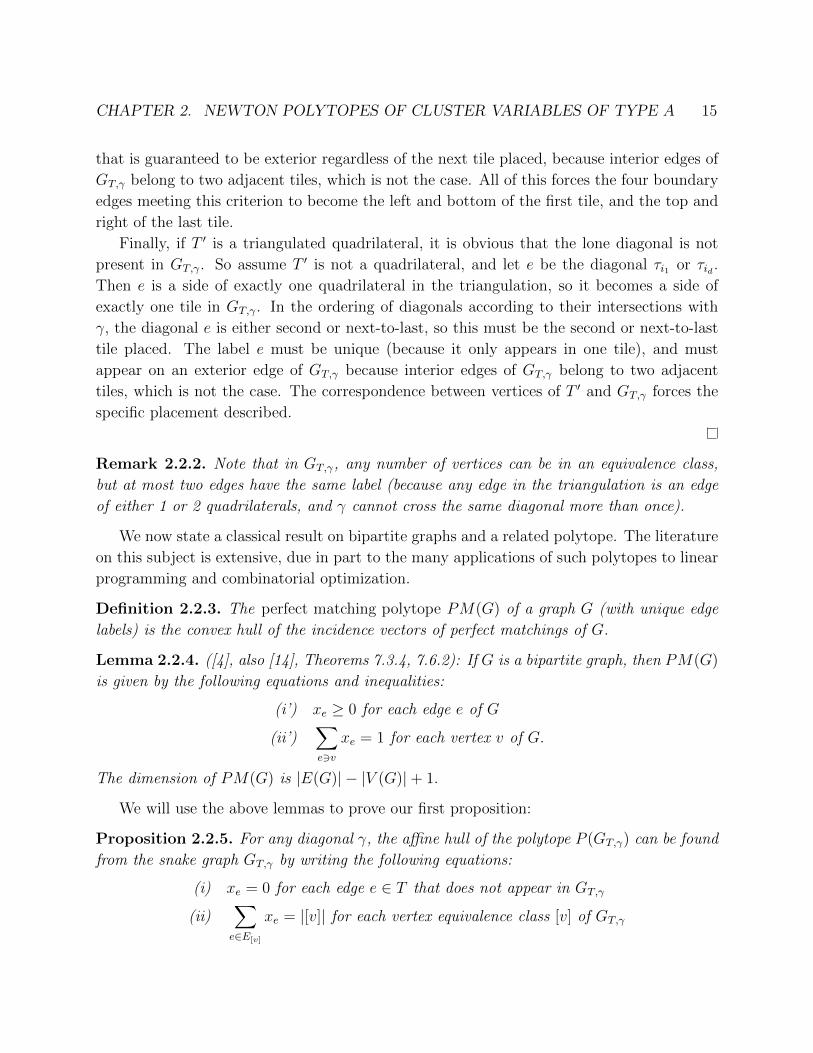
Proposition 2.2.5. For any diagonal γ, the affine hull of the polytope P (GT,γ) can be found
from the snake graph GT,γ by writing the following equations:
(i) xe = 0 for each edge e ∈ T that does not appear in GT,γ
(ii)∑e∈E[v]
xe = |[v]| for each vertex equivalence class [v] of GT,γ

CHAPTER 2. NEWTON POLYTOPES OF CLUSTER VARIABLES OF TYPE A 16
Using the triangulation T directly, the equivalent equations are
(iii) xe = 0 for each edge e of T\T ′
(iv)∑e3w
xe = |diagonals(w)| for each vertex w of T ′
The equations defining the affine hull here (either (i)-(ii) or (iii)-(iv)) are linearly inde-
pendent, and thus are a minimal description of the affine hull. There are 2n + 3 − |D(γ)|equations in this minimal description.
Proof. Proposition 2.2.5 will follow immediately from the three statements that follow (Lemma
2.2.6, Lemma 2.2.7, and Proposition 2.2.8).
Lemma 2.2.6. The set of equations (iii)-(iv) consists of 2n+3−|D(γ)| linearly independent
equations.
Proof. Suppose some linear combination of the sums on the left-hand sides of equations (iv)
equals zero: ∑w∈T ′
(cw∑e3w
xe
)= 0 (2.1)
Here, the outer sum runs over each vertex w of T ′. Choose a diagonal that forms a triangle
with two boundary segments of T ′, and label it 1. Without loss of generality, we can label
T ′ as in this figure:!
E
D
C
B
A
1
2
3
4 5
Note that each edge label in T ′ appears in exactly two sums in Proposition 2.2.5(iv) (the
equations corresponding to the two endpoints of that edge). We can thus collect the terms
of equation (2.1) so that the coefficient of xedge(w1,w2) is cw1 + cw2 (see above figure):
(cA + cC)x1 + (cA + cB)x2 + (cB + cC)x3 + ... = 0. (2.2)
Since all coefficients in equation (2.2) must be zero, we can reason as follows. First, since
cA + cC = cA + cB = cB + cC = 0, we can conclude that cA = cB = cC = 0. Now, the next

CHAPTER 2. NEWTON POLYTOPES OF CLUSTER VARIABLES OF TYPE A 17
term in equation (2.2) is (cC + cD)x4, so (cC + cD) must be zero. But we know cC = 0, so
this forces cD = 0. This knowledge in turn forces cE = 0, and so on until all cw are zero.
Thus the equations (iv) are linearly independent.
Clearly, the equations (iii) are linearly independent from each other, and also are linearly
independent from those in (iv) because they involve different variables. So indeed (iii) and
(iv) together form a linearly independent set.
Next we will prove that there are 2n+ 3− |D(γ)| equations in this description (iii)-(iv).
Observe that the set of edges of the triangulation T can be partitioned into three subsets:
edges of T = edges of T\T ′ t boundary segments of T ′ t D(γ).
Taking cardinalities, this equation becomes
2n+ 3 = # of edges of T\T ′ + # of vertices in T ′ + |D(γ)|. This is
2n+ 3 = # of equations in (iii) + # of equations in (iv) + |D(γ)|, as desired.
Lemma 2.2.7. The set of equations (i)-(ii) is equivalent to the set of equations (iii)-(iv).
Proof. We will consider the cases |D(γ)| ≥ 2 and |D(γ)| = 1 separately.
Suppose first that |D(γ)| ≥ 2. Note that GT,γ is constructed from T ′, so any edge e that
is not in T ′ does not appear in GT,γ. Conversely, since |D(γ)| ≥ 2, every edge that is in T ′
is the side of a quadrilateral in T ′, so it appears in GT,γ. Thus (i) is equivalent to (iii).
We will show that by the construction of the snake graph as a gluing of tiles isotopic to
quadrilaterals in the triangulation, (ii) is equivalent to (iv). Comparing the two statements,
we need to show that each vertex equivalence class [v] of GT,γ corresponds to a vertex w of
T ′, that the labels of edges incident to [v] in GT,γ are the same as the labels of edges incident
to the corresponding w in T ′, and that |[v]| = |diagonals(w)|. There are 2 cases to consider.
Case 1: Vertex w ∈ T ′ is incident to γ. Then it is not incident to any diagonals in T ′,
so diagonals(w) = {γ}. In this case, w is a vertex of exactly 1 quadrilateral in T ′, which
becomes exactly 1 tile in GT,γ, and so there is exactly 1 vertex v in the snake graph GT,γ
corresponding to w. The labels of the two edges incident to w in T ′ clearly become the labels
of the two edges incident to v in the tile that becomes embedded in GT,γ. Since w is not part
of any other quadrilateral in T ′, the corresponding vertex v ∈ GT,γ only appears in this tile
in the snake graph, and the next tile is glued onto it along an edge that does not include v.
Thus no more edges can become incident to v ∈ GT,γ when this next tile is glued on. So the
labels of edges incident to v ∈ GT,γ are precisely the same as the labels of edges incident to
the corresponding w ∈ T ′, as desired. Also, in this case |[v]| = 1 = |{γ}| = |diagonals(w)|.Case 2: Vertex w ∈ T ′ is not incident to γ. Then, since |D(γ)| ≥ 2, w is a vertex of
at least 2 quadrilaterals in T ′. Also, |diagonals(w)| = number of diagonals in D(γ) that

CHAPTER 2. NEWTON POLYTOPES OF CLUSTER VARIABLES OF TYPE A 18
are incident to w. Each of these diagonals is the diagonal of a unique quadrilateral in
T ′. After deletion of the diagonal, each of these quadrilaterals becomes a tile in the snake
graph GT,γ, and since w cannot be on the shared (i.e. glued) edge of any two of these
quadrilaterals, the vertex corresponding to w in one tile does not coincide with the vertex
corresponding to w in another tile when the tiles are glued together to form the snake graph.
Since all the vertices corresponding to w remain distinct when GT,γ is formed, there are
exactly |diagonals(w)| vertices in GT,γ that correspond to w. In this way, w corresponds to
an entire equivalence class [v] of vertices of GT,γ, and this equivalence class has cardinality
|diagonals(w)|, as desired. Let m be the label of an edge in T ′ incident to w. There are at
least 2 quadrilaterals in T ′ incident to w, so m must be the side of some quadrilateral, hence
it becomes an edge in GT,γ that is incident to some vertex in GT,γ that corresponds to w.
Conversely, if m is the label of an edge in GT,γ incident to a vertex of GT,γ that corresponds
to w, then it is the side of a quadrilateral in T ′ with a vertex at w, hence it is the label of an
edge in T ′ incident to w. So indeed the labels of edges incident to [v] in GT,γ are the same
as the labels of edges incident to the corresponding w in T ′.
We have considered both cases, so (ii) is indeed equivalent to (iv). Thus (i)-(ii) is equiv-
alent to (iii)-(iv) for the case |D(γ)| ≥ 2.
If |D(γ)| = 1, then T ′ is a triangulated quadrilateral. We can label the lone crossed
diagonal 1, and the four sides 2, 3, 4, and 5, counterclockwise, such that the vertices are
incident to edges {1, 2, 5}, {2, 3}, {1, 3, 4}, and {4, 5}. Then the equations given by (i)-(iv)
are as follows:
(i) x1 = 0
(ii) x2 + x5 = 1;x2 + x3 = 1;x3 + x4 = 1;x4 + x5 = 1
(iii) [none]
(iv) x1 + x2 + x5 = 1;x2 + x3 = 1;x1 + x3 + x4 = 1;x4 + x5 = 1
Here, the set of equations (i)-(ii) clearly implies (iii)-(iv), and in fact (iii)-(iv) implies (i)-(ii)
as well (alternately add and subtract the equations in (iv) for example). Thus the equations
(i)-(ii) is equivalent to the set of equations (iii)-(iv).
Proposition 2.2.8. The set of equations (i)-(ii) describes the affine hull of P (GT,γ).
Proof. We will define a new graph as well as a projection map.
Say the edge labels of GT,γ are 1..k. Without loss of generality, say that edge labels
{1, ..., r} occur on two distinct edges, and edge labels {r + 1, ..., k} appear uniquely. (Note
that by Remark 2.2.2, the same edge label cannot appear more than twice in GT,γ, so those
are the only two possibilities.)
Define a graph G to be the graph GT,γ, but with edges labeled in the following way.
For each edge label e that is unique in GT,γ, label the corresponding edge of G with that
same label e. For each edge label e that is found on two distinct edges in GT,γ, label the

CHAPTER 2. NEWTON POLYTOPES OF CLUSTER VARIABLES OF TYPE A 19
corresponding edges of G as e and k + e. Now G is a graph that has the same structure as
GT,γ, but with unique edge labels. Therefore Lemma 2.2.4 applies to G.
Define a projection π : Rk+r → Rk by
(x1, ..., xk+r) 7→ (x1 + xk+1, ..., xr + xk+r, xr+1, ...xk).
This projection maps edge weight vectors of G onto the corresponding edge weight vectors of
GT,γ, based on the above labeling scheme. Note that the projection respects the equivalence
relation on vertices and edges of GT,γ defined earlier. Also note that the polytope P (GT,γ)
is simply the image of PM(G) under the map π.
Now we can address our equations (i) and (ii). Note that the cluster expansion formula
in Proposition 1.3.3 is based on GT,γ, so any edge e that is not in GT,γ does not appear
in the cluster expansion. Hence every such xe must be 0, so the equations (i) are true for
P (GT,γ). For (ii), note that the polytope P (GT,γ) is simply the image of PM(G) under
the map π. Adding together equations in Lemma 2.2.4(ii’) that correspond to equivalent
vertices and then applying π, we get our equations (ii), so our equations (ii) are clearly true
for P (GT,γ). We now need only show that the equations (i)-(ii) are also sufficient (i.e. no
others are needed).
By Lemma 2.2.4, dim PM(G) = |E(G)| − |V (G)|+ 1. By the construction of the snake
graph, this quantity is exactly the number of boxes in the graph, which is d. (Induction: the
graph G has the same structure as GT,γ, which consists of d boxes glued together. With 1
box, the formula from Lemma 2.2.4 gives dim PM(G) = 1. Each added box increases the
number of vertices by 2 and the number of edges by 3, so |E(G)|−|V (G)|+1 (the dimension)
increases by 1. By induction, dim PM(G) = d.) Recall that in our case of the polygon,
d = |D(γ)|, so we have dim PM(G) = |D(γ)|.Recall that P (GT,γ) was defined as a polytope in R2n+3. From Lemmas 2.2.6 and 2.2.7, we
already know that (i)-(ii) consists of (or is equivalent to) 2n+3−|D(γ)| linearly independent
hyperplanes, each of which cuts down (by 1) the dimension of the affine subspace that
P (GT,γ) lives in. Subtracting, we see that no more equations are needed if and only if the
dimension of the affine hull of P (GT,γ) is exactly |D(γ)|.So we need to show that the projection map π preserves the dimension of PM(G).
Instead of working directly with the affine hull of PM(G) (an affine subspace of R3n+1),
we will work instead with Q, the linear subspace that is given by writing the equations in
Lemma 2.2.4(ii’) with a 0 on the right-hand side instead of a 1. So Q is just the affine hull of
PM(G), but shifted so it passes through the origin. We will show that dim π(Q) = dim Q.
(It suffices to show this instead because if T is any linear transformation of a space S, then
T (S +−→OP ) = T (S) +
−−−−−→O T (P ), which clearly has the same dimension as T (S).)
First we will define a basis for Q. We will imagine an element of Q as an assignment of
weights to the edges of the graph G such that the sum of the weights of edges incident to each

CHAPTER 2. NEWTON POLYTOPES OF CLUSTER VARIABLES OF TYPE A 20
vertex is 0. By the above paragraph, we need to find |D(γ)| linearly independent vectors in
Q. Define qi to be the following assignment of edge weights: weight 1 on the horizontal edges
of the ith box in the snake graph, weight −1 on the vertical edges of the ith box, and weight
0 on all other edges (see figure below for what q2 looks like in our example). Since there are
|D(γ)| boxes in G, and these edge weights are linearly independent by construction, the qiform a basis for Q.
Next we will define a basis for ker π. Again, we imagine a vector here as an assignment
of weights to the edges of the graph G. For 1 ≤ i ≤ r, define bi to be following assignment of
edge weights: weight 1 on the edge labeled i, weight −1 on the edge labeled k+ i, and weight
0 on all other edges. See the figure below for what b4 looks like in our example (note: here,
the basis is {b3, b4, b5} rather than “{b1, b2, b3}” because we did not relabel the non-unique
edges, but it doesn’t matter). This is well-defined since at most two edges collapse to the
same label under π, and the pairs of edges that do collapse are precisely the ones involved
here. The bi here clearly form a basis for ker π. q2 =
-1
0
0
0 0
0
1 0 0 0
0 -1
1 0 0
0
b4 =
0
0
0
0 0
0
1 0 0 0
0 0
0 0 -1
0
Now we will show that the bi (basis vectors of ker π) are all linearly independent from
the qi (basis vectors of Q). Suppose a linear combination∑
i ciqi + dibi = 0. Note that all
interior edges on the bi have weight 0. The leftmost edge of box 1 is nonzero only in q1,
forcing c1 = 0. The edge of box 2 that touches box 1 is nonzero only in q2 (forcing c2 = 0),
or in q1 and q2 (forcing c2 = −c1 = 0). Either way, c2 = 0. Similarly, the edge of box 3 that
touches box 2 is nonzero only in q3, or in q2 and q3, forcing c3 = 0. Continuing in this way, we
see that all ci = 0. Now, the bi are already linearly independent, so all di must be 0 as well.
Therefore, we have shown that the basis vectors for ker π are indeed linearly independent
from the basis vectors of Q. From this we can conclude that dim π(Q) = dim Q.
Thus dim P (GT,γ) = dim π(PM(G)) = dim π(Q) = dim Q = dim PM(G) = |D(γ)|, so
no more equations are needed and we are done.
Corollary 2.2.9. dim N(T, γ) = dim P (GT,γ) = |D(γ)|.
Proof. The dimension of P (GT,γ) was discussed in the proof of Lemma 2.2.8. The equality
with dim N(T, γ) simply follows from Remark 2.1.3.

CHAPTER 2. NEWTON POLYTOPES OF CLUSTER VARIABLES OF TYPE A 21
Example 2.2.10. Using the same example as in Figure 1.3, we will illustrate Proposition
2.2.5 and Corollary 2.2.9. Our computations were made or checked with the help of the
software polymake [12] and Mathematica.
• (i)-(ii): Since edges 14 and 15 of T do not appear in GT,γ, the affine hull of P (GT,γ)
includes the equations x14 = 0 and x15 = 0. The other equations defining the affine hull
of P (GT,γ) come from each of the equivalence classes of vertices of GT,γ. For example,
the equivalence class {a, a′, a′′} has cardinality 3, and the edges of GT,γ incident to those
vertices are labeled 1, 2, 3, 4, and 7, so we get the equation x1 + x2 + x3 + x4 + x7 = 3.
• (iii)-(iv): We can get the same list of equations as above by using T directly. Since
edges 14 and 15 of T do not appear in T ′, we again get the equations x14 = 0 and
x15 = 0. The other equations defining the affine hull of P (GT,γ) come from each vertex
of T ′. For example, the edges incident to vertex A are {1, 2, 3, 4, 7}, three of which
({2, 3, 4}) are in γ ∪D(γ), so we get the equation x1 + x2 + x3 + x4 + x7 = 3.
• Since we are triangulating a 9-gon, n = 6. Also, D(γ) = {2, 3, 4, 5, 6}, so dim N(T, γ) =
|D(γ)| = 5. The number of equations defining the affine hull is 2n+ 3− |D(γ)| = 10.
So here are the 10 equations for the affine hull of P (GT,γ) (using either (i)-(ii) or (iii)-(iv)).
The reader may check that they form a linearly independent set.
absent edge 14: x14 = 0
absent edge 15: x15 = 0
{a, a′, a′′} or A : x1 + x2 + x3 + x4 + x7 = 3
{b, b′} or B : x5 + x6 + x7 + x8 = 2
{c} or C : x8 + x9 = 1
{d} or D : x6 + x9 + x10 = 1
{e, e′} or E : x4 + x5 + x10 + x11 = 2
{f} or F : x3 + x11 + x12 = 1
{g} or G : x2 + x12 + x13 = 1
{h} or H : x1 + x13 = 1
We now need another classic result from the literature on bipartite graphs and matching
polytopes.
Lemma 2.2.11. ([1] 2.1): Denote the complete bipartite graph by Kn,n. The face lattice of
the Birkhoff polytope PM(Kn,n) is isomorphic to the lattice of elementary subgraphs of Kn,n
ordered by inclusion.

CHAPTER 2. NEWTON POLYTOPES OF CLUSTER VARIABLES OF TYPE A 22
Remark 2.2.12. The isomorphism of lattices described in Lemma 2.2.11 still holds when
Kn,n is replaced with any elementary subgraph of Kn,n. Specifically, if H is an elementary
subgraph of Kn,n, then under this isomorphism it corresponds to a face F of Kn,n, and any
elementary subgraph of H corresponds to a face of F , so the face lattice of F is isomorphic
to the lattice of elementary subgraphs of H. Also note that our graph G is an elementary
subgraph of Kn,n, and PM(G) is a face of Kn,n.
Theorem 2.2.13. The face lattice of N(T, γ) (and of P (GT,γ)) is isomorphic to the lattice
of all elementary subgraphs of GT,γ, ordered by inclusion.
Proof. Note that P (GT,γ) is the image of PM(G) under the projection map π defined in
the proof of Proposition 2.2.8. Since the two polytopes have the same dimension, |D(γ)|,and π is a linear transformation, P (GT,γ) must be combinatorially isomorphic to PM(G).
By Remark 2.1.3, N(T, γ) is a translate of P (GT,γ), so the face lattice of N(T, γ) must
be isomorphic to the face lattice of PM(G). But G is an elementary subgraph of Kn,n,
so by Remark 2.2.12, the face lattice of PM(G) is isomorphic to the lattice of elementary
subgraphs of G, which is clearly isomorphic to the lattice of elementary subgraphs of GT,γ,
and we are done.
Corollary 2.2.14. The following are in one-to-one correspondence:
(i) Laurent monomials in the T -expansion of xγ
(ii) perfect matchings of GT,γ
(iii) vertices of N(T, γ)
Proof. Every vertex is an atom in the face lattice of N(T, γ), and every perfect matching of
GT,γ is an atom in the elementary subgraph lattice, so Theorem 2.2.13 implies that vertices
of N(T, γ) correspond one-to-one with perfect matchings of GT,γ.
Now, every distinct Laurent monomial in the T -expansion of xγ gives one distinct point
that is either a vertex of N(T, γ) or not. If not a vertex, then there is no perfect matching
corresponding to that monomial. But that contradicts the formula in Proposition 1.3.3 that
says that every monomial comes from a perfect matching. Therefore Laurent monomials
correspond one-to-one with vertices.
Example 2.2.15. Using the same example as Figure 1.3, we will illustrate Corollary 2.2.14.
One Laurent monomial in the T -expansion of xγ can be written asx1x2x3x25x9x2x3x4x5x6
.
This corresponds to the N(T, γ) vertex (1, 0, 0,−1, 1,−1, 0, 0, 1, 0, 0, 0, 0, 0, 0) and the perfect
matching here:

CHAPTER 2. NEWTON POLYTOPES OF CLUSTER VARIABLES OF TYPE A 23
2
13
1
7 8
3
4 5 6 9
10 11
12 5 4
3
The lattices described in Theorem 2.2.13 are graded: the rank of a face is 1 more than its
dimension, and the rank of an elementary subgraph is 1 more than the number of chordless
cycles it contains. So the d-faces of N(T, γ) are in bijection with elementary subgraphs of
GT,γ containing exactly d chordless cycles (these cycles may or may not be disjoint).
In particular, let P (i) be the perfect matching of GT,γ that corresponds to vertex i of
the polytope. Given a set of vertices (i1, . . . , ir) that make up a face, the corresponding
elementary subgraph is obtained by superimposing P (i1), . . . , P (ir). Conversely, given an
elementary subgraph H, if the set of all perfect matchings of GT,γ that lie entirely on H
is P (i1), . . . , P (ir), then (i1, . . . , ir) is the set of vertices making up the corresponding face.
Note that to count only the number of vertices making up a face, we need only count the
number of perfect matchings of the “cycle part” of H (i.e. the union of all the cycles in H),
since the rest of H is already matched.
Also, in particular, the facets of N(T, γ) are the (n − 1)-faces, so they can be found by
finding the elementary subgraphs of GT,γ containing n− 1 chordless cycles. We will do this
below.
Example 2.2.16. We will illustrate Theorem 2.2.13 using a small example. Let T be a
triangulation of a pentagon, with γ a diagonal that crosses both diagonals of T . Then GT,γ
consists of two boxes, and the face lattice of N(T, γ) is isomorphic to the following lattice of
elementary subgraphs of GT,γ.
In this example, the dimension of N(T, γ) is |D(γ)| = 2, and N(T, γ) is a triangle. Also
note that the length of every maximal chain in this lattice is 3.

CHAPTER 2. NEWTON POLYTOPES OF CLUSTER VARIABLES OF TYPE A 24
GT,γ =
Figure 2.1: Lattice of Elementary Subgraphs of GT,γ
Example 2.2.17. Theorem 2.2.13 can be used to find the f -vector of N(T, γ), by count-
ing how many elementary subgraphs contain d chordless cycles for each d from 0 to |D(γ)|−1.
For example, the f -vector of N(T, γ) from our original example in Figure 1.3 is (11, 31, 39, 25, 8).
We now turn our attention to the facets of our Newton polytopes.
Proposition 2.2.18. For any diagonal γ, the facets of the polytope P (GT,γ) can be found
from the snake graph GT,γ by writing the following inequalities:
(i) xe ≥ 0 for each e ∈ GT,γ such that e is an interior edge of GT,γ.
(ii) xe ≥ 0 for each pair of opposite exterior edges {e, f} of GT,γ such that at least one
of the two edges has a label e that is unique in GT,γ. (see figure below)
(iii) xa + xb + xc ≤ 2 for each pair of opposite exterior edges {e, f} of GT,γ that includes
no unique labels, where a, b and c are the labels of edges shown in the figure below. GT,γ =
a
e a
b
f
c
Remark 2.2.19. Details of Proposition 2.2.18:
• In (ii), if both of the opposite exterior edges are unique labels in GT,γ (only possible if
T ′ is a triangulated quadrilateral or triangulated pentagon), arbitrarily choose one to
be e.
CHAPTER 2. NEWTON POLYTOPES OF CLUSTER VARIABLES OF TYPE A 25
• The pair of edges {e, f} in (ii) happens precisely on the first, second, penultimate, and
last tile of GT,γ (the ones of these that are not corners). The pair of edges {e, f} in
(iii) happens on all other tiles in GT,γ that are not corners. This follows from Lemma
2.2.1.
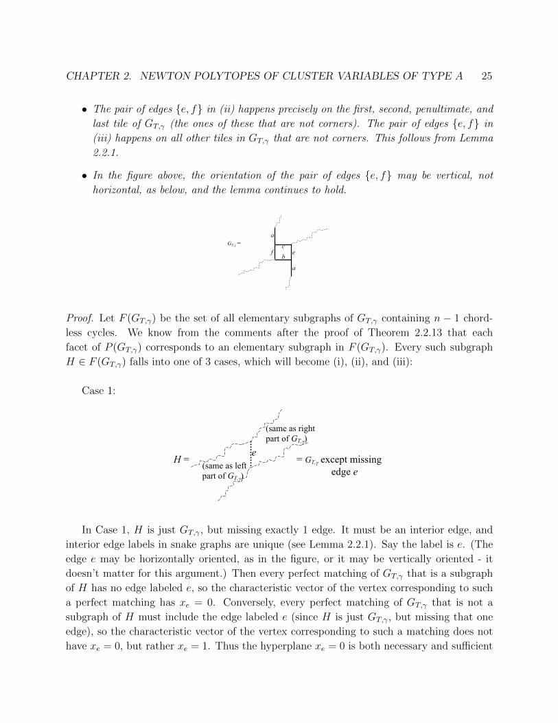
• In the figure above, the orientation of the pair of edges {e, f} may be vertical, not
horizontal, as below, and the lemma continues to hold. GT,γ =
a
b
a
f c
e
Proof. Let F (GT,γ) be the set of all elementary subgraphs of GT,γ containing n − 1 chord-
less cycles. We know from the comments after the proof of Theorem 2.2.13 that each
facet of P (GT,γ) corresponds to an elementary subgraph in F (GT,γ). Every such subgraph
H ∈ F (GT,γ) falls into one of 3 cases, which will become (i), (ii), and (iii):
Case 1: H = = GT,γ except missing
edge e
e (same as left part of GT,γ)
(same as right part of GT,γ)
In Case 1, H is just GT,γ, but missing exactly 1 edge. It must be an interior edge, and
interior edge labels in snake graphs are unique (see Lemma 2.2.1). Say the label is e. (The
edge e may be horizontally oriented, as in the figure, or it may be vertically oriented - it
doesn’t matter for this argument.) Then every perfect matching of GT,γ that is a subgraph
of H has no edge labeled e, so the characteristic vector of the vertex corresponding to such
a perfect matching has xe = 0. Conversely, every perfect matching of GT,γ that is not a
subgraph of H must include the edge labeled e (since H is just GT,γ, but missing that one
edge), so the characteristic vector of the vertex corresponding to such a matching does not
have xe = 0, but rather xe = 1. Thus the hyperplane xe = 0 is both necessary and sufficient
CHAPTER 2. NEWTON POLYTOPES OF CLUSTER VARIABLES OF TYPE A 26
- it includes all the desired vertices and no others. This confirms (i).
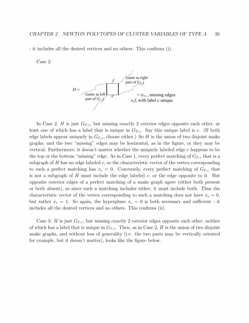
Case 2: H =
= GT,γ , missing edges e,f, with label e unique
e
f
(same as left part of GT,γ)
(same as right part of GT,γ)
In Case 2, H is just GT,γ, but missing exactly 2 exterior edges opposite each other, at
least one of which has a label that is unique in GT,γ. Say this unique label is e. (If both
edge labels appear uniquely in GT,γ, choose either.) So H is the union of two disjoint snake
graphs, and the two “missing” edges may be horizontal, as in the figure, or they may be
vertical. Furthermore, it doesn’t matter whether the uniquely labeled edge e happens to be
the top or the bottom “missing” edge. As in Case 1, every perfect matching of GT,γ that is a
subgraph of H has no edge labeled e, so the characteristic vector of the vertex corresponding
to such a perfect matching has xe = 0. Conversely, every perfect matching of GT,γ that
is not a subgraph of H must include the edge labeled e, or the edge opposite to it. But
opposite exterior edges of a perfect matching of a snake graph agree (either both present
or both absent), so since such a matching includes either, it must include both. Thus the
characteristic vector of the vertex corresponding to such a matching does not have xe = 0,
but rather xe = 1. So again, the hyperplane xe = 0 is both necessary and sufficient - it
includes all the desired vertices and no others. This confirms (ii).
Case 3: H is just GT,γ, but missing exactly 2 exterior edges opposite each other, neither
of which has a label that is unique in GT,γ. Then, as in Case 2, H is the union of two disjoint
snake graphs, and without loss of generality (i.e. the two parts may be vertically oriented
for example, but it doesn’t matter), looks like the figure below.

CHAPTER 2. NEWTON POLYTOPES OF CLUSTER VARIABLES OF TYPE A 27 H = = GT,γ , missing
opposite exterior edges with no unique labels
a
a
b c (same as right part of GT,γ) (same as left
part of GT,γ)
Note that the construction of snake graphs (or the comments about vertex equivalence
earlier in this paper) guarantees the two edges labeled a do indeed have the same label,
and that no other edges of GT,γ are labeled a. Also note that the edges labeled b and c are
interior edges of GT,γ, so they are uniquely labeled. Every perfect matching of GT,γ that is
a subgraph of H looks locally like one of four types:

CHAPTER 2. NEWTON POLYTOPES OF CLUSTER VARIABLES OF TYPE A 28
Type 1: :
Type 2: :
a
a
b c
xa = 2 xb = 0 xc = 0
a
a
b c xa = 0 xb = 1 xc = 1
Type 3: :
Type 4: :
xa = 1 xb = 0 xc = 1
a
a
b c
a
a
b c xa = 1 xb = 1 xc = 0
In each of these 4 cases, it is true that xa+xb+xc = 2. Conversely, every perfect matching
of GT,γ that is not a subgraph of H must include both edges of GT,γ\H, so it cannot include
any edge labeled a, b, or c, hence xa+xb+xc = 0, not 2. Thus the hyperplane xa+xb+xc = 2
is both necessary and sufficient - it includes all the desired vertices and no others. This case
proves that (iii) gives a facet, and the direction of inequality that defines the half-space is
clear.
Corollary 2.2.20. If |D(γ)| ≥ 2, the number of facets of N(T, γ) (or P (GT,γ)) is 2d−1− t,where t is the number of corners in the snake graph, or equivalently, the number of imbalanced
diagonals in T ′. (If |D(γ)| = 1, the polytope is a line segment, so it has 2 facets that are the
endpoints.)
Proof. Assume |D(γ)| ≥ 2. First note that by Lemma 2.2.1, the number of imbalanced
diagonals in T ′ is the number of corners in GT,γ, so it is valid to call them both t. The
number of interior edges of GT,γ is 1 less than the number of boxes, so Proposition 2.2.18(i)
gives d−1 facets. Combining Proposition 2.2.18(ii)-(iii), we see that we get 1 facet for every
CHAPTER 2. NEWTON POLYTOPES OF CLUSTER VARIABLES OF TYPE A 29
pair of opposite exterior edges, and since |D(γ)| ≥ 2, there are at least two boxes in GT,γ,
so there is clearly 1 pair of opposite exterior edges for every box that is not at a corner in
the graph. The number of such boxes not at a corner is d − t. Adding d − 1 to d − t gives
the desired result.
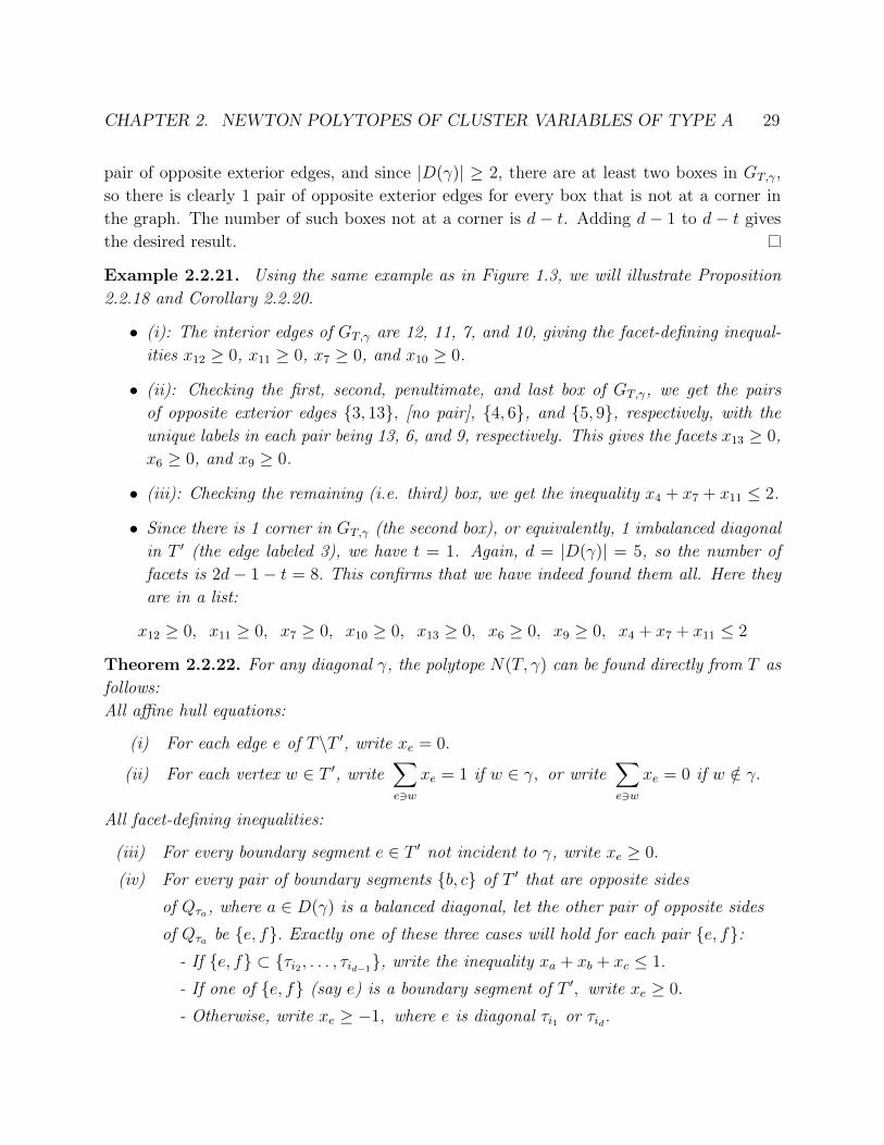
Example 2.2.21. Using the same example as in Figure 1.3, we will illustrate Proposition
2.2.18 and Corollary 2.2.20.
• (i): The interior edges of GT,γ are 12, 11, 7, and 10, giving the facet-defining inequal-
ities x12 ≥ 0, x11 ≥ 0, x7 ≥ 0, and x10 ≥ 0.
• (ii): Checking the first, second, penultimate, and last box of GT,γ, we get the pairs
of opposite exterior edges {3, 13}, [no pair], {4, 6}, and {5, 9}, respectively, with the
unique labels in each pair being 13, 6, and 9, respectively. This gives the facets x13 ≥ 0,
x6 ≥ 0, and x9 ≥ 0.
• (iii): Checking the remaining (i.e. third) box, we get the inequality x4 + x7 + x11 ≤ 2.
• Since there is 1 corner in GT,γ (the second box), or equivalently, 1 imbalanced diagonal
in T ′ (the edge labeled 3), we have t = 1. Again, d = |D(γ)| = 5, so the number of
facets is 2d− 1− t = 8. This confirms that we have indeed found them all. Here they
are in a list:
x12 ≥ 0, x11 ≥ 0, x7 ≥ 0, x10 ≥ 0, x13 ≥ 0, x6 ≥ 0, x9 ≥ 0, x4 + x7 + x11 ≤ 2
Theorem 2.2.22. For any diagonal γ, the polytope N(T, γ) can be found directly from T as
follows:
All affine hull equations:
(i) For each edge e of T\T ′, write xe = 0.
(ii) For each vertex w ∈ T ′, write∑e3w
xe = 1 if w ∈ γ, or write∑e3w
xe = 0 if w /∈ γ.
All facet-defining inequalities:
(iii) For every boundary segment e ∈ T ′ not incident to γ, write xe ≥ 0.
(iv) For every pair of boundary segments {b, c} of T ′ that are opposite sides
of Qτa, where a ∈ D(γ) is a balanced diagonal, let the other pair of opposite sides
of Qτa be {e, f}. Exactly one of these three cases will hold for each pair {e, f}:- If {e, f} ⊂ {τi2 , . . . , τid−1
}, write the inequality xa + xb + xc ≤ 1.
- If one of {e, f} (say e) is a boundary segment of T ′, write xe ≥ 0.
- Otherwise, write xe ≥ −1, where e is diagonal τi1 or τid .

CHAPTER 2. NEWTON POLYTOPES OF CLUSTER VARIABLES OF TYPE A 30
Proof. This proof will follow from previous propositions and the shift of 1 unit downward in
the direction of each of the crossed diagonals D(γ) described in Remark 2.1.3. Specifically,
statement (i) was proven in Proposition 2.2.5, and is not affected by the shift.
For statement (ii), we will shift the variables from Proposition 2.2.5(iv). The 1 unit
downward translation means that each instance of xe should be replaced with (xe + 1) if
e ∈ D(γ), and left as xe if e /∈ D(γ). Modifying Proposition 2.2.5(iv) in this way, we get
|{e ∈ D(γ) : e 3 w}|+∑w3e
xe = |diagonals(w)|.
If w is not incident to γ, then {e ∈ D(γ) : e 3 w} is diagonals(w) by definition, so canceling in
the above equation, we get∑
w3e xe = 0. If w is incident to γ, then |{e ∈ D(γ) : e 3 w}| = 0,
while |diagonals(w)| = 1, so we get∑
e∈Ewxe = 1. Thus our new right-hand side is 0 if w is
not incident to γ and 1 if w is incident to γ.
For statement (iii), refer to Lemma 2.2.1 and Proposition 2.2.18. Specifically, boundary
segments of T ′ that are not incident to γ become interior edges of GT,γ when the snake graph
is formed, and boundary segments are not affected by the shift, so Proposition 2.2.18(i) proves
(iii).
To prove the first case of (iv), suppose in Qτa we have a pair of opposite sides that are
boundary segments of T ′, and both of the other two sides {e, f} are in the set {τi2 , . . . , τid−1}.
Then by Lemma 2.2.1, their labels are not unique in GT,γ, and by the construction of the
snake graph, e and f form opposite exterior edges of a tile in GT,γ that has a as the deleted
diagonal, b and c as the other two sides, and flanking edges a and a (see figure in Proposition
2.2.18). This places us exactly in the situation of statement (iii) of Proposition 2.2.18. Of
sides a, b, and c, only a corresponds to a crossed diagonal, so replacing xa with xa + 1 in
Proposition 2.2.18(iii) proves the desired inequality that forms the first case.
To prove the second and third cases of (iv), suppose in Qτa we have a pair of opposite
sides that are boundary segments of T ′, and at least one of the other two sides {e, f} (without
loss of generality, say e) is not a diagonal in the set {τi2 , . . . , τid−1}. By Lemma 2.2.1, e is
a unique label in GT,γ. Again, by construction of the snake graph, e and f form opposite
exterior edges of a tile in GT,γ that has a as the deleted diagonal, b and c as the other two
sides, and flanking edges a and a (see figure in Proposition 2.2.18). This places us exactly
in the situation of statement (ii) of Proposition 2.2.18. If e is a boundary segment, then it
is not affected by the shift, so Proposition 2.2.18(ii) proves the second case inequality. If e
is diagonal τi1 or τid , then it is affected by the shift of 1 unit downward, so replacing xe with
xe + 1 in Proposition 2.2.18(ii) gives the third case inequality.
Example 2.2.23. Using the same example as in Figure 1.3, we will illustrate Theorem
2.2.22.

CHAPTER 2. NEWTON POLYTOPES OF CLUSTER VARIABLES OF TYPE A 31
• (i): Since edges 14 and 15 of T do not appear in T ′, we get x14 = 0 and x15 = 0.
• (ii): The other equations defining the affine hull of N(T, γ) come from each vertex of
T ′ and whether they are incident to γ. For example, the edges incident to vertex A are
{1, 2, 3, 4, 7}, and A is not incident to γ, so we get the equation x1+x2+x3+x4+x7 = 0.
• (iii): Edges 7, 10, 11, and 12 are boundary segments of the triangulated polygon T ′
that are not incident to γ, so we get x7 ≥ 0, x10 ≥ 0, x11 ≥ 0, x12 ≥ 0.
• (iv): The pairs of boundary segments of T ′ that are opposite sides of Qτa, where a is
a balanced diagonal in D(γ), are {1, 12}, {7, 11}, {7, 10}, and {8, 10}. The other pairs
of opposite sides of each quadrilateral are, respectively, {3, 13},{3, 5}, {4, 6}, and {5, 9}. Since {τi1 , τi2 , . . . , τid−1
, τid} = {2, 3, 4, 5, 6}, these pairs fall
into the following cases:
– Both of {3, 5} are in {τi2 , . . . , τid−1}. They are sides of Qτ4, whose other two sides
are 7 and 11. This gives x4 + x7 + x11 ≤ 1.
– The edge 13 is a boundary segment of T ′, so {3, 13} gives x13 ≥ 0. Similarly,
{5, 9} gives x9 ≥ 0.
– The edges {4, 6} are not both in {τi2 , . . . , τid−1}, nor is either one a boundary
segment of T ′, so we get x6 ≥ −1.
Putting this all together, the affine hull and facets of N(T, γ) are given by
affine hull: x14 = 0, x15 = 0
A : x1 + x2 + x3 + x4 + x7 = 0 B : x5 + x6 + x7 + x8 = 0
C : x8 + x9 = 1 D : x6 + x9 + x10 = 0
E : x4 + x5 + x10 + x11 = 0 F : x3 + x11 + x12 = 0
G : x2 + x12 + x13 = 0 H : x1 + x13 = 1
facets: x7 ≥ 0, x10 ≥ 0, x11 ≥ 0, x12 ≥ 0,
x13 ≥ 0, x9 ≥ 0, x6 ≥ −1, x4 + x7 + x11 ≤ 1
Note that Corollary 2.2.20 confirms that we have found all the facets (as computed above,
the number of facets is 2d− 1− t = 2(5)− 1− 1 = 8.)
As mentioned earlier, an important application of matching polytopes of bipartite graphs
relates to combinatorial optimization. In the specific case of Theorem 2.2.22, we have a short
description of all equations and inequalities that define the [shifted version of the] perfect
matching polytope of the snake graph. This may prove useful in optimization, as follows.

CHAPTER 2. NEWTON POLYTOPES OF CLUSTER VARIABLES OF TYPE A 32
Suppose weights (costs) are assigned to the labels of edges of a snake graph, and we
wish to find the perfect matching that minimizes total cost. Equivalently, suppose costs are
assigned to the boundary segments and diagonals of a triangulated polygon, and we wish to
find the T -path (see [22]) from one vertex to another that minimizes total cost. For small
cases, a brute force approach is reasonable: simply try every matching (or T -path) and pick
the cheapest one. But the number of matchings grows exponentially with the number of
crossed diagonals, so this approach is not scalable to larger problems.
For a scalable approach, note that minimization of total cost across all matchings is
simply tropicalization of the Laurent expansion of the cluster variable associated with that
set of matchings or T -paths. (By tropicalization, we mean replace x + y with min(x, y),
and replace x · y with x + y.) The affine hull and facet description of the [shifted] perfect
matching polytope in Theorem 2.2.22 can be interpreted as a set of constraints that defines
the feasible region of the linear programming problem of minimizing the cost function. (To
be clear, the cost function here is f(x) = cTx, where c is the vector of costs.) The number
of such constraints only grows linearly with the size of the polygon or snake graph, and so
this optimization problem can be solved in polynomial time using well-known algorithms.

33
Chapter 3
Other Results and Conjectures
Section 3.2 is joint work with Steven Karp.
3.1 Remarks for Type A
If all the frozen variables {xn+1, ..., x2n+3} (i.e. boundary segments of the polygon) are set
equal to 1, the Newton polytope N(T, γ) is less elegant - there is a collapsing of monomials
in the cluster expansion, and not every monomial corresponds to a vertex. For example, let
T be the triangulated hexagon below. T = γ
1 2
3
4
5
6
7
8
9
The corresponding snake graph is a 2-by-4 square grid graph. The T -expansion of xγ is
x22x5x8 + x2x4x6x8 + x1x3x6x9 + x2x5x7x9 + x4x6x7x9
x1x2x3
and N(T, γ) is 3-dimensional with 5 vertices. These numbers correspond neatly to the
3 crossed diagonals and 5 terms in the numerator, as well as the 3 boxes and 5 perfect
matchings of the corresponding snake graph.
CHAPTER 3. OTHER RESULTS AND CONJECTURES 34
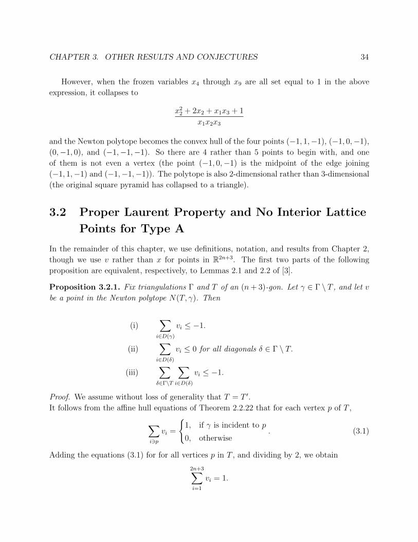
However, when the frozen variables x4 through x9 are all set equal to 1 in the above
expression, it collapses to
x22 + 2x2 + x1x3 + 1
x1x2x3
and the Newton polytope becomes the convex hull of the four points (−1, 1,−1), (−1, 0,−1),
(0,−1, 0), and (−1,−1,−1). So there are 4 rather than 5 points to begin with, and one
of them is not even a vertex (the point (−1, 0,−1) is the midpoint of the edge joining
(−1, 1,−1) and (−1,−1,−1)). The polytope is also 2-dimensional rather than 3-dimensional
(the original square pyramid has collapsed to a triangle).
3.2 Proper Laurent Property and No Interior Lattice
Points for Type A
In the remainder of this chapter, we use definitions, notation, and results from Chapter 2,
though we use v rather than x for points in R2n+3. The first two parts of the following
proposition are equivalent, respectively, to Lemmas 2.1 and 2.2 of [3].
Proposition 3.2.1. Fix triangulations Γ and T of an (n+ 3)-gon. Let γ ∈ Γ \ T , and let v
be a point in the Newton polytope N(T, γ). Then
(i)∑i∈D(γ)
vi ≤ −1.
(ii)∑i∈D(δ)
vi ≤ 0 for all diagonals δ ∈ Γ \ T.
(iii)∑δ∈Γ\T
∑i∈D(δ)
vi ≤ −1.
Proof. We assume without loss of generality that T = T ′.
It follows from the affine hull equations of Theorem 2.2.22 that for each vertex p of T ,
∑i3p
vi =
{1, if γ is incident to p
0, otherwise. (3.1)
Adding the equations (3.1) for for all vertices p in T , and dividing by 2, we obtain
2n+3∑i=1
vi = 1.
CHAPTER 3. OTHER RESULTS AND CONJECTURES 35
Partition the edges in T into three sets: D(γ), B = the four boundary segments of the
polygon which are incident to γ, and C = all remaining edges. Then the left-hand side
above breaks into three sums: ∑i∈D(γ)
vi +∑i∈B
vi +∑i∈C
vi = 1.
But adding the equations (3.1) for the two vertices that are the endpoints of γ, we see that
the second sum is 2. This implies that∑i∈D(γ)
vi +∑i∈C
vi = −1.
Now, from the snake graph expansion formula in Proposition 1.3.3, we get that vi ≥ 0 for
i /∈ D(γ). Hence∑
i∈C vi ≥ 0, and (i) follows immediately.
To prove (ii), let δ be any diagonal in Γ \ (T ∪ {γ}). Observe that δ is compatible with
γ, so we can orient the triangulation so that δ is to the left of γ. Adding the equations (3.1)
for all vertices p in T which are strictly to the left of δ, we obtain∑i∈D(δ)
vi +∑
i weakly left of δ
civi = 0 (ci ∈ {1, 2}).
Note that any edge weakly left of δ cannot be inD(γ). But from the formula from Proposition
1.3.3, vi ≥ 0 for i /∈ D(γ). Hence the second sum above is nonnegative, and (ii) follows.
Inequality (iii) now follows from adding inequality (i) to the inequalities (ii) for all δ ∈Γ \ (T ∪ {γ}).
The geometric interpretation of inequality (iii) above is that for any triangulation Γ,
each Newton polytope N(T, γ) (for γ ∈ Γ \ T ) is strictly separated from the nonnegative
orthant by a common hyperplane through the origin. The equation of this hyperplane in
R2n+3 is∑
δ∈Γ\T∑
i∈D(δ) vi = 0. Visually, we can write down this equation by superimposing
triangulations Γ and T . The coefficient of vi on the left-hand side is 0 unless i ∈ T \ Γ, in
which case it equals the number of γ ∈ Γ \ T which cross i.
The following corollary establishes that the same hyperplane separates the Newton poly-
tope of any cluster monomial from the nonnegative orthant, providing a partial generalization
of Proposition 3.6 in [23]. This establishes that A(QT ) has the proper Laurent property.
Corollary 3.2.2. Suppose that {γ1, . . . , γn} is the set of diagonals of triangulation Γ, and
x = xk1γ1 . . . xknγn is a cluster monomial, where k1, . . . , kn ≥ 0 and kj > 0 for some γj ∈ Γ \ T .
Then every point v in the Newton polytope of the T -expansion of x satisfies∑δ∈Γ\T
∑i∈D(δ)
vi < 0, (3.2)

CHAPTER 3. OTHER RESULTS AND CONJECTURES 36
whence every Laurent monomial has a variable xi (for some i ∈ T \ Γ) with a negative
exponent. In particular, A(QT ) has the proper Laurent property.
Proof. The Newton polytope for x is the Minkowski sum of the Newton polytopes for
xk1γ1 , . . . , xknγn , and in turn the Newton polytope of xkiγi is ki times the Newton polytope of
xγi . Hence it suffices to show that each of the Newton polytopes of xγi (1 ≤ i ≤ n) lies
weakly on the negative side of the separating hyperplane, and strictly on the negative side
if i = j. If γi /∈ T (including i = j), this follows from Proposition 3.2.1(iii). If γi ∈ T ,
then the Newton polytope N(T, γi) is the point {ei}, and the point ei lies on the separating
hyperplane.
Now let m be a Laurent monomial in the T -expansion of x, corresponding to a point v
in the Newton polytope of x. By equation (3.2), vi < 0 for some i ∈ T \ Γ, whence the
exponent of xi in m is negative.
We have shown that each Newton polytope is strictly separated from the nonnegative
orthant by a common hyperplane through the origin, and used this to prove that A(QT ) has
the proper Laurent property. Note that by the Hahn-Banach theorem we can reverse the
argument, i.e. if a cluster algebra A has the proper Laurent property, then such a common
separating hyperplane exists. To see this, let u, u′ be (primary) seeds of A, and for every
cluster monomial m in u′ \ u = {y1, . . . , ys}, let N(m) denote the Newton polytope of the
Laurent expanion of m in u \ u′. Then we have the chain of equivalent statements
N(yk11 . . . ykss ) ∩ Rs≥0 = ∅ for k ∈ Ns \ {0}
⇐⇒ (k1N(y1) + · · ·+ ksN(ys)) ∩ Rs≥0 = ∅ for k ∈ Ns \ {0}
⇐⇒(
k1
k1 + · · ·+ ksN(y1) + · · ·+ ks
k1 + · · ·+ ksN(ys)
)∩ Rs
≥0 = ∅ for k ∈ Ns \ {0}
⇐⇒ (λ1N(y1) + · · ·+ λsN(ys)) ∩ Rs≥0 = ∅ for λ1, . . . , λs ≥ 0, λ1 + · · ·+ λs = 1
⇐⇒ Conv(N(y1), . . . , N(ys)) is strictly separated from Rs≥0 by a hyperplane
⇐⇒ N(y1), . . . , N(ys) are strictly separated from Rs≥0 by a common hyperplane.
We will now transition to examining the relative interior of these Newton polytopes.
Let ρ : R2n+3 → Rn be the projection which fixes each coordinate corresponding to a
cluster variable. We now consider ρ(N(T, γ)), which is the Newton polytope of the Laurent
expansion of xγ in T after setting all coefficient variables to 1. Since ρ(relint(N(T, γ))) ⊆relint(ρ(N(T, γ))) and ρ(Z2n+3) = Zn, in order to show that N(T, γ) has no relative interior
lattice points it suffices to show that ρ(N(T, γ)) has no relative interior lattice points. The
only cases in which the latter fails (as we now show) are when γ ∈ T , in which case N(T, γ)

CHAPTER 3. OTHER RESULTS AND CONJECTURES 37
is a lattice point (and is its own relative interior), or when n = 1 and γ /∈ T , in which case
N(T, γ) is a line segment with no relative interior lattice points which projects to a lattice
point.
Proposition 3.2.3. Suppose that n ≥ 2 and γ is a diagonal not in T . Then ρ(N(T, γ)) has
no lattice points in its relative interior (and hence neither does N(T, γ)).
Proof. We consider 2 cases.
Case 1 (|D(γ)| = 1). Write D(γ) = {i}. Then flipping the diagonal i gives γ, and the
corresponding exchange relation is xixγ = xaxd + xbxc, where a, b, c, d ∈ [2n+ 3] are distinct
and at least one of xa, xb, xc, xd is a cluster variable (since n ≥ 2). Hence ρ(N(T, γ)) =
Conv({u − ei, v − ei}), where u, v ∈ {0, 1}n are distinct, and so ρ(N(T, γ)) has no interior
lattice points.
Case 2 (|D(γ)| ≥ 2). Let u ∈ N(T, γ) such that ρ(u) ∈ Zn. We will show that ρ(u)
is not in the relative interior of ρ(N(T, γ)). By 3.2.1(i) we have∑
i∈D(γ) ui ≤ −1, and
by assumption ui ∈ Z for i ∈ D(γ), so uj ≤ −1 for some j ∈ D(γ). Now note that in
the snake graph expansion from Proposition 1.3.3, xj appears in the denominator exactly
once. Hence vj ≥ −1 for all v ∈ N(T, γ). On the other hand, j labels some edge of the
snake graph (since |D(γ)| ≥ 2), and each edge of the snake graph is used in some perfect
matching M , so tj ≥ 0 for some t ∈ N(T, γ). Then ρ(u) + λ(ρ(t) − ρ(u)) ∈ ρ(N(T, γ))
for λ ∈ [0, 1] (by convexity), but ρ(u) + λ(ρ(t) − ρ(u)) /∈ ρ(N(T, γ)) for λ < 0 (since
(ρ(u) + λ(ρ(t)− ρ(u)))j = (u+ λ(t− u))j < −1).
As a final result of this section, we used Polymake to refute the conjecture that every
lattice point of N(T, γ) is a vertex, and to refute the conjecture that N(T, γ) is Gorenstein.
A lattice polytope is one whose vertices are lattice points. A reflexive polytope is a
lattice polytope whose dual is a lattice polytope. One property of a reflexive polytope is
that it contains exactly one interior lattice point, the origin. A Gorenstein polytope is a
lattice polytope P such that kP + v is reflexive for some integer k > 0 and lattice point
v. Equivalently, P is Gorenstein if and only if its h∗-polynomial has symmetric coefficients.
Note that if a polytope is not Gorenstein, it is not reflexive.
For a counterexample to both conjectures, consider the cluster algebra coming from a
heptagon with vertices labeled 1 through 7, counterclockwise, with diagonals connecting the
pairs of vertices {{1, 3}, {1, 4}, {1, 5}, {5, 7}}. Let γ be the arc that crosses all four of these
diagonals.
Then N(T, γ) has 7 vertices and 14 lattice points, so not every lattice point of N(T, γ)
is a vertex. Also, 3N(T, γ) has no relative interior lattice points, while 4N(T, γ) has
exactly 2 relative interior lattice points (namely (1,−2,−2,−1,−3, 3, 1, 1, 1, 3, 1, 2)T and

CHAPTER 3. OTHER RESULTS AND CONJECTURES 38
(1,−2,−2, 0,−3, 3, 1, 1, 1, 2, 2, 1)T ), so N(T, γ) is not Gorenstein. Alternatively, the h∗-
polynomial of N(T, γ) is 1 + 2t, which does not have symmetric coefficients.
3.3 Remarks and Conjectures for Other Cluster
Algebras
The construction of cluster algebras from triangulations of a polygon may be generalized
to construct cluster algebras from triangulations of an arbitrary surface with marked points
([5, 6, 7, 13, 8]). In this setting, there is a generalization of the Laurent expansion formula
using perfect matchings of snake graphs ([16, 17, 18]). Empirically, many of the results of
this paper do not hold when a more general surface is considered. For example, consider the
annulus and corresponding snake graph that serves as the example in [16], Section 7:
!
1
2
3
4
5 6 7 8
γ
D
A
B
C
a
a'
a'''
a'''
b
b'
d
d'
c
c'
c''
c''''
c'''
a'' 1
1
2
2 2
3
3
3
4
4
4
1
5
5
6
6
7
8
8
Figure 3.1: Example from [16], Section 7
There are 17 matchings of the snake graph in Figure 3.1, but these 17 matchings give
only 13 distinct monomials, because two different matchings may give the same monomial.
For example, there are two different matchings that both give the monomial x1x2x3x24x5x8.
Therefore, there can be no bijection between matchings and vertices of GT,γ. Moreover,
there is no bijection between Laurent monomials and vertices either, because when these

CHAPTER 3. OTHER RESULTS AND CONJECTURES 39
13 distinct monomials are used to form the Newton polytope, only 9 of them correspond to
vertices. So overall, our result on the isomorphism of lattices does not hold for more general
surfaces. Using the principal coefficient system instead for this example, the same collapsing
occurs, even if we leave all x−variables and y−variables as they are, setting nothing equal
to 1.
For surfaces other than a polygon, our results concerning the facets are not valid, and
our affine hull description in Theorem 2.2.22(i)-(ii) seems only partially complete, in that the
theorem seems to give some of the affine hull equations, but not necessarily all of them. In
the future, we hope to have a complete affine hull and facet description for cluster variables
from more general surfaces.
We may also be able to obtain results for cluster algebras not from surfaces in certain
cases. For example, there is a procedure called folding that relates type C cluster algebras
to type A cluster algebras (see [15]). There are also known geometric realizations of type C
cluster algebras based on centrally symmetric triangulations of the n-gon. Moreover, it can
be shown that the cluster expansion formulas based on perfect matchings of snake graphs
can be modified to provide Laurent expansions for type C. These approaches provide a map
from type A cluster variables to type C cluster variables, which induces a map of type A
Newton polytopes to type C Newton polytopes. We hope to work out all the details of this
approach in the future.
40
Chapter 4
Code and Visualizations
4.1 Code and Output
The results in this thesis are theoretical, but the research itself involved a lot of computer
experimentation to come up with and test conjectures. To do this, I wrote code in Math-
ematica to compute cluster variables and points in Rn and used Polymake to analyze the
convex hull. What follows on the next few pages is the relevant Mathematica code.

CHAPTER 4. CODE AND VISUALIZATIONS 41
Functions and Procedures
This loads the Combinatorica package.
In[1]:= << Combinatorica`
The function mutatecluster[cluster, exchange_matrix, position_k] returns a new cluster by mutating the kth variable in thecluster based on the exchange matrix. It is a straightforward implemenation of the exchange relation.
In[2]:= mutatecluster@x_, b_, k_D := Module@8posprod, negprod, i<,posprod = 1; negprod = 1;For@i = 1, i § Length@bD,If@b@@i, kDD > 0, posprod = posprod * x@@iDD^b@@i, kDD, negprod = negprod * x@@iDD^-b@@i, kDDD; i++D;
ReplacePart@x, k Ø Together@Hposprod + negprodL ê x@@kDDDDD
The function mutatematrix[exchange_matrix, position_k] returns a new exchange matrix by mutating at row k and column k.It works for square matrices and for rectangular matrices with more rows than columns. It is a straightforward implementation ofthe matrix mutation formula for skew-symmetric cluster algebras.
In[3]:= mutatematrix@b_, k_D := Module@8m, i, j<,m = ConstantArray@0, Dimensions@bDD;For@i = 1, i § Length@mD,For@j = 1, j § Dimensions@mD@@2DD,If@i == k »» j == k, m@@i, jDD = -b@@i, jDD,m@@i, jDD = b@@i, jDD + Sign@b@@i, kDDD Max@b@@i, kDD b@@k, jDD, 0DD
; j++D; i++D;mD
The function affineSubspaceDim[list_of_points] computes the dimension of the affine subspace spanned by a set of points.
In[4]:= affineSubspaceDim@pointlist_D :=MatrixRank@Map@Ò - First@pointlistD &, pointlistDD;
In what follows, the vertices of the polygon are numbered counterclockwise from 1 to ngon. Diagonals are represented as a pairof vertices. A triangulation is represented as a list of diagonals.
The function flip[triangulation, position_k] returns the diagonal that is the flip of the kth diagonal in the triangulation.
In[5]:= flip@triangulation_, k_D := Module@8edges, n<,n = Length@triangulationD + 3;edges = Join@triangulation, Transpose@8Range@nD, RotateLeft@Range@nDD<DD;Complement@Intersection@Flatten@
Select@edges, Ò@@1DD ã triangulation@@k, 1DD »» Ò@@2DD ã triangulation@@k, 1DD &DD,Flatten@Select@edges, Ò@@1DD ã triangulation@@k, 2DD »»
Ò@@2DD ã triangulation@@k, 2DD &DDD, triangulation@@kDDDD
code for dissertation.nb 1
Printed by Mathematica for Students
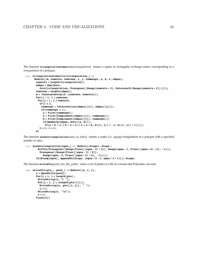
CHAPTER 4. CODE AND VISUALIZATIONS 42
The function triangulationtomatrix[triangulation] returns a square or rectangular exchange matrix corresponding to atriangulation of a polygon.
In[6]:= triangulationtomatrix@triangulation_D :=Module@8m, numcols, numrows, i, j, commonpt, a, b, c, edges<,numcols = Length@triangulationD;edges = Map@Sort,
Join@triangulation, Transpose@8Range@numcols + 3D, RotateLeft@Range@numcols + 3DD<DDD;numrows = Length@edgesD;m = ConstantArray@0, 8numrows, numcols<D;For@i = 1, i § numrows,For@j = 1, j § numcols,If@i ! j,commonpt = Intersection@edges@@iDD, edges@@jDDD;If@commonpt ! 8<,c = First@commonptD;a = First@Complement@edges@@iDD, commonptDD;b = First@Complement@edges@@jDD, commonptDD;If@MemberQ@edges, Sort@8a, b<DD,If@a < b < c »» b < c < a »» c < a < b, m@@i, jDD = -1, m@@i, jDD = 1DDDD;
j++D; i++D;mD
The function snaketriangulation[num_of_sides] returns a snake (i.e. zigzag) triangulation of a polygon with a specifiednumber of sides.
In[7]:= snaketriangulation@ngon_D := Module@8diags<, diags =Riffle@Transpose@8Range@Floor@Hngon - 3L ê 2DD, Range@ngon - 1, Floor@Hngon + 4L ê 2D, -1D<D,Transpose@8Range@Floor@Hngon - 3L ê 2DD,
Range@ngon - 2, Floor@Hngon + 2L ê 2D, -1D<DD;If@EvenQ@ngonD, AppendTo@diags, 8ngon ê 2 - 1, ngon ê 2 + 1<DD; diagsD
The function writePts[point_list, file_path] writes a set of points to a file in a format that Polymake can read.
In[8]:= writePts@pts_, path_D := Module@8s, i, j<,s = OpenWrite@pathD;For@i = 1, i § Length@ptsD,WriteString@s, "1 "D;For@j = 1, j § Length@pts@@1DDD,WriteString@s, pts@@i, jDD, " "D;j++D;
WriteString@s, "\n"D;i++D;
Close@sDD
code for dissertation.nb 2
Printed by Mathematica for Students
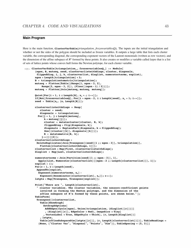
CHAPTER 4. CODE AND VISUALIZATIONS 43
Main Program
Here is the main function, ClusterVarTable[triangulation, frozenvariablesQ]. The inputs are the initial triangulation andwhether or not the sides of the polygon should be included as frozen variables. It outputs a large table that lists each clustervariable, the corresponding diagonal, the corresponding exponent vectors of the Laurent monomials (written as row vectors), andthe dimension of the affine subspace of Rn formed by these points. It also creates or modifies a variable called latpts that is a listof sets of lattice points whose convex hull forms the Newton polytope, for each cluster variable.
In[9]:= ClusterVarTable@triangulation_, frozenvariablesQ_D := Module@8ngon, B, mutseq, seed, clustervarlistwithdiags, cluster, diagonals,flippeddiag, i, j, k, clustervarlist, diaglist, numeratorterms, explist<,
ngon = Length@triangulationD + 3;B = triangulationtomatrix@triangulationD;mutseq = Flatten@Table@8Range@1, ngon - 3, 2D,
Range@2, ngon - 3, 2D<, 8Floor@Hngon - 1L ê 2D<DD;mutseq = Flatten@Join@mutseq, mutseq, mutseqDD;
Quiet@For@i = 1, i § Length@BD, xi =.; i++DD;If@Not@frozenvariablesQD, For@i = ngon - 2, i § Length@seedD, xi = 1; i++DD;seed = Table@xn, 8n, Length@BD<D;
clustervarlistwithdiags = Reap@cluster = seed;diagonals = triangulation;
For@j = 1, j § Length@mutseqD,k = mutseq@@jDD;cluster = mutatecluster@cluster, B, kD;flippeddiag = flip@diagonals, kD;diagonals = ReplacePart@diagonals, k Ø flippeddiagD;Sow@8cluster@@kDD, diagonals@@kDD<D;B = mutatematrix@B, kD;
j++DD@@2DD;clustervarlistwithdiags =DeleteDuplicates@Join@Transpose@8seed@@1 ;; ngon - 3DD, triangulation<D,
Flatten@clustervarlistwithdiags, 1DDD;clustervarlist = Map@First, clustervarlistwithdiagsD;diaglist = Map@Last, clustervarlistwithdiagsD;
numeratorterms = Join@Partition@seed@@1 ;; ngon - 3DD, 1D,Apply@List, Numerator@clustervarlistD@@ngon - 2 ;; Length@clustervarlistDDD, 1DD;
explist = 8<;For@c = 1, c § Length@seedD,AppendTo@explist,Exponent@numeratorterms, xcD -Exponent@Denominator@clustervarlistD, xcDD; c++D;
latpts = Map@Transpose, Transpose@explistDD;
Print@"There are ", Length@clustervarlistD," cluster variables. The cluster variables, the nonzero-coefficient points
involved in forming the Newton polytope, and the dimension of theaffine subspace of R^n formed by these points, are shown below." D;
TableForm@Transpose@8clustervarlist,
Table@ShowGraph@SetGraphOptions@AddEdges@Cycle@ngonD, Union@triangulation, 8diaglist@@rDD<DD, 8diaglist@@rDD, EdgeColor Ø Red<, ImageSize Ø TinyD
, VertexLabel Ø True, EdgeStyle Ø ThickD, 8r, Length@diaglistD<D, latpts,Table@affineSubspaceDim@latpts@@rDDD, 8r, Length@clustervarlistD<D<D, TableHeadings Ø
8None, 8"Cluster Var", "Diagonal", "Points", "Dim"<<, TableSpacing Ø 85, 3<DD
Here is an example of ClusterVarTable.
code for dissertation.nb 3
Printed by Mathematica for Students
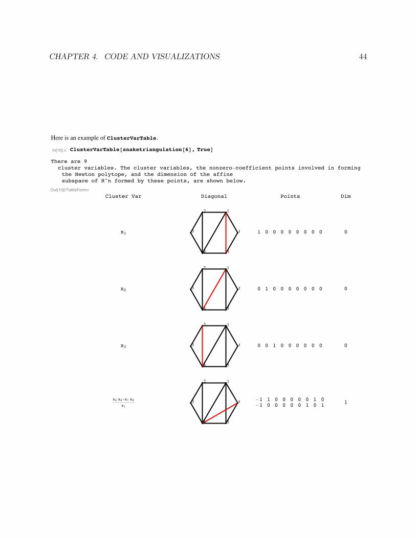
CHAPTER 4. CODE AND VISUALIZATIONS 44
Here is an example of ClusterVarTable.
In[10]:= ClusterVarTable@snaketriangulation@6D, TrueD
There are 9cluster variables. The cluster variables, the nonzero-coefficient points involved in formingthe Newton polytope, and the dimension of the affinesubspace of R^n formed by these points, are shown below.
Out[10]//TableForm=Cluster Var Diagonal Points Dim
x1
12
3
4 5
6 1 0 0 0 0 0 0 0 0 0
x2
12
3
4 5
6 0 1 0 0 0 0 0 0 0 0
x3
12
3
4 5
6 0 0 1 0 0 0 0 0 0 0
x2 x8+x7 x9
x1
12
3
4 5
6 -1 1 0 0 0 0 0 1 0-1 0 0 0 0 0 1 0 1
1
code for dissertation.nb 4
Printed by Mathematica for Students

CHAPTER 4. CODE AND VISUALIZATIONS 45
x2 x5+x4 x6
x3
12
3
4 5
6 0 1 -1 0 1 0 0 0 00 0 -1 1 0 1 0 0 0 1
x22 x5 x8+x2 x4 x6 x8+x1 x3 x6 x9+x2 x5 x7 x9+x4 x6 x7 x9
x1 x2 x3
12
3
4 5
6
-1 1 -1 0 1 0 0 1 0-1 0 -1 1 0 1 0 1 00 -1 0 0 0 1 0 0 1-1 0 -1 0 1 0 1 0 1-1 -1 -1 1 0 1 1 0 1
3
x1 x3 x6+x2 x5 x7+x4 x6 x7
x2 x3
12
3
4 5
61 -1 0 0 0 1 0 0 00 0 -1 0 1 0 1 0 00 -1 -1 1 0 1 1 0 0
2
x2 x4 x8+x1 x3 x9+x4 x7 x9
x1 x2
12
3
4 5
6-1 0 0 1 0 0 0 1 00 -1 1 0 0 0 0 0 1-1 -1 0 1 0 0 1 0 1
2
x1 x3+x4 x7
x2
12
3
4 5
6 1 -1 1 0 0 0 0 0 00 -1 0 1 0 0 1 0 0 1
code for dissertation.nb 5
Printed by Mathematica for Students

CHAPTER 4. CODE AND VISUALIZATIONS 46
Interaction of Mathematica and Polymake
The table created by ClusterVarTable lists the dimension of each Newton polytope. To find out more about this polytope (e.g.f-vector, facets) requires specialized software such as Polymake. Here we prepare to analyze the 6th row of the large table aboveby creating a file called "points.txt" that stores the coordinates of the points whose convex hull we want to study.
In[11]:= writePts@latpts@@6DD, "êUsersêadamkalmanêDesktopêpoints.txt"D
Out[11]= êUsersêadamkalmanêDesktopêpoints.txt
To read from the file on the desktop named "points.txt," we can copy and paste this into Polymake:
open(INPUT, "</Users/adamkalman/Desktop/points.txt");$matrix = new Matrix<Rational>(<INPUT>);close(INPUT);$p = new Polytope(POINTS=>$matrix);
Some Polymake commands that proved useful over the course of this research are
$p=new Polytope<Rational>;$p->POINTS=<<"."; (use if entering points manually) print($p->N_VERTICES," vertices, ",$p->N_FACETS," facets, ",$p->DIM," dimensions"); print("f-vector: ", $p->F_VECTOR); print("affine hull: ", $p->AFFINE_HULL); print("facets: ", $p->FACETS); print("vertices: ", $p->VERTICES); print("h-vector: ", $p->H_VECTOR); print rows_labeled($p->GRAPH->ADJACENCY); print("congruent? 1=yes, 0=no: ", congruent($p,$q)); print("# of lattice points incl. boundary: ", $p->N_LATTICE_POINTS); print("# of strictly interior lattice points:" $p->INTERIOR_LATTICE_POINTS); print $p->EHRHART_POLYNOMIAL_COEFF; print $p->VOLUME; print $p->H_STAR_VECTOR; print $p->LATTICE_DEGREE; print $p->LATTICE_CODEGREE; print $p->LATTICE_VOLUME; print $p->REFLEXIVE; $HD = $p->HASSE_DIAGRAM; for (my $k=$HD->DIMS->[0];$k<$HD->DIMS->[1]; ++$k) { print $HD->FACES->[$k] }; for (my $k=$HD->DIMS->[1];$k<$HD->DIMS->[2]; ++$k) { print $HD->FACES->[$k] }; for (my $k=$HD->DIMS->[2];$k<$HD->DIMS->[3]; ++$k) { print $HD->FACES->[$k] }; for (my $k=$HD->DIMS->[3];$k<$HD->DIMS->[4]; ++$k) { print $HD->FACES->[$k] }; for (my $k=$HD->DIMS->[4];$k<$HD->DIMS->[5]; ++$k) { print $HD->FACES->[$k] }; $inequalities=new Matrix<Rational>([
[0,1,0,0,0,0,0,0,0,0],...[1,0,0,0,0,-1,-1,0,0,0]]);$p=new Polytope<Rational>(INEQUALITIES=>$inequalities);
print_constraints($inequalities);
A useful Mathematica command that reads the "points.txt" file back into a list of points in Mathematica format is
In[12]:= ReadList@"êUsersêadamkalmanêDesktopêpoints.txt", Number, RecordLists -> TrueD;Transpose@Rest@Transpose@%DDD
Out[13]= 88-1, 1, -1, 0, 1, 0, 0, 1, 0<, 8-1, 0, -1, 1, 0, 1, 0, 1, 0<,80, -1, 0, 0, 0, 1, 0, 0, 1<, 8-1, 0, -1, 0, 1, 0, 1, 0, 1<, 8-1, -1, -1, 1, 0, 1, 1, 0, 1<<
code for dissertation.nb 6
Printed by Mathematica for Students

47
Bibliography
[1] Billera, Louis J. and Sarangarajan, A. “The combinatorics of permutation polytopes”.
In: Formal power series and algebraic combinatorics (New Brunswick, NJ, 1994).
Vol. 24. DIMACS Ser. Discrete Math. Theoret. Comput. Sci. Amer. Math. Soc., Prov-
idence, RI, 1996, 1–23.
[2] G. Carroll and G. Price. “Two new combinatorial models for the Ptolemy recurrence”.
2003.
[3] Dupont, Gregoire and Thomas, Hugh. “Atomic bases of cluster algebras of types A
and A”. In: Proc. Lond. Math. Soc. (3) 107.4 (2013), 825–850.
[4] Edmonds, Jack. “Paths, trees, and flowers”. In: Canad. J. Math. 17 (1965), 449–467.
[5] Fock, Vladimir and Goncharov, Alexander. “Moduli spaces of local systems and higher
Teichmuller theory”. In: Publ. Math. Inst. Hautes Etudes Sci. 103 (2006), 1–211.
[6] Fock, Vladimir V. and Goncharov, Alexander B. “Cluster ensembles, quantization and
the dilogarithm”. In: Ann. Sci. Ec. Norm. Super. (4) 6 (2009), 865–930.
[7] Fock, Vladimir V. and Goncharov, Alexander B. “Dual Teichmuller and lamination
spaces”. In: Handbook of Teichmuller theory. Vol. I. Vol. 11. IRMA Lect. Math. Theor.
Phys. Eur. Math. Soc., Zurich, 2007, 647–684.
[8] Fomin, Sergey and Shapiro, Michael and Thurston, Dylan. “Cluster algebras and tri-
angulated surfaces. I. Cluster complexes”. In: Acta Math. 201.1 (2008), 83–146.
[9] Fomin, Sergey and Zelevinsky, Andrei. “Cluster algebras. I. Foundations”. In: J. Amer.
Math. Soc. 15.2 (2002), 497–529 (electronic).
[10] Fomin, Sergey and Zelevinsky, Andrei. “Cluster algebras. II. Finite type classification”.
In: Invent. Math. 154.1 (2003), 63–121.
[11] Fomin, Sergey and Zelevinsky, Andrei. “Cluster algebras. IV. Coefficients”. In: Compos.
Math. 143.1 (2007), 112–164.
BIBLIOGRAPHY 48
[12] Ewgenij Gawrilow and Michael Joswig. polymake: a framework for analyzing convex
polytopes. Polytopes-combinatorics and computation (Oberwolfach, 1997), 43-73, DMV
Sem., 29, Birkhauser, Basel. 2000.
[13] Gekhtman, Michael and Shapiro, Michael and Vainshtein, Alek. “Cluster algebras and
Weil-Petersson forms”. In: Duke Math. J. 127.2 (2005), 291–311.
[14] Lovasz, L. and Plummer, M. D. Matching theory. Vol. 121. North-Holland Mathemat-
ics Studies. North-Holland Publishing Co., Amsterdam; Akademiai Kiado (Publishing
House of the Hungarian Academy of Sciences), Budapest, 1986.
[15] Marsh, Robert J. Lecture notes on cluster algebras. Zurich Lectures in Advanced Math-
ematics. European Mathematical Society (EMS), Zurich, 2013.
[16] Musiker, Gregg and Schiffler, Ralf. “Cluster expansion formulas and perfect match-
ings”. In: J. Algebraic Combin. 32.2 (2010), 187–209.
[17] Musiker, Gregg and Schiffler, Ralf and Williams, Lauren. “Bases for cluster algebras
from surfaces”. In: Compos. Math. 149.2 (2013), 217–263.
[18] Musiker, Gregg and Schiffler, Ralf and Williams, Lauren. “Positivity for cluster alge-
bras from surfaces”. In: Adv. Math. 227.6 (2011), 2241–2308.
[19] James Propp. “The combinatorics of frieze patterns and Markoff numbers”. In: arXiv:
math.CO/0511633 (2005).
[20] Schiffler, Ralf. “A cluster expansion formula (An case)”. In: Electron. J. Combin. 15.1
(2008), Research paper 64, 9.
[21] Schiffler, Ralf. “On cluster algebras arising from unpunctured surfaces. II”. In: Adv.
Math. 223.6 (2010), 1885–1923.
[22] Schiffler, Ralf and Thomas, Hugh. “On cluster algebras arising from unpunctured sur-
faces”. In: Int. Math. Res. Not. IMRN 17 (2009), 3160–3189.
[23] Sherman, Paul and Zelevinsky, Andrei. “Positivity and canonical bases in rank 2 cluster
algebras of finite and affine types”. In: Mosc. Math. J. 4.4 (2004), 947–974, 982.
Recommended