Download pdf - Multivariate Statistics: Grouped Multivariate Data and ...ams.med.uni-goettingen.de/download/Steffen-Unkel/chap2.pdf · Hotelling’s T2 test Multivariate analysis of variance (MANOVA)

Hotelling’s T2 testMultivariate analysis of variance (MANOVA)

Discriminant analysisFurther classification functions

Multivariate Statistics: Grouped Multivariate Dataand Discriminant Analysis

Steffen Unkel

Department of Medical StatisticsUniversity Medical Center Goettingen, Germany

Summer term 2017 1/38



Univariate test for equality of means of two variables

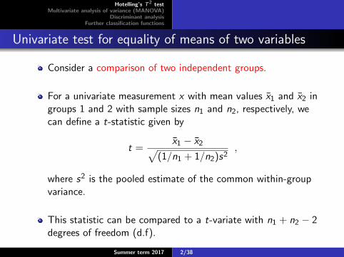
Consider a comparison of two independent groups.

For a univariate measurement x with mean values x1 and x2 ingroups 1 and 2 with sample sizes n1 and n2, respectively, wecan define a t-statistic given by

t =x1 − x2√

(1/n1 + 1/n2)s2,

where s2 is the pooled estimate of the common within-groupvariance.

This statistic can be compared to a t-variate with n1 + n2 − 2degrees of freedom (d.f).




Multivariate analogue

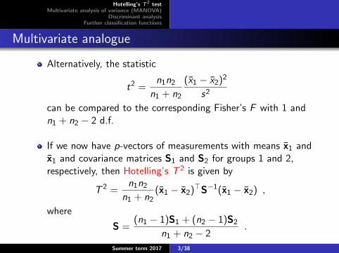
Alternatively, the statistic

t2 =n1n2

n1 + n2

(x1 − x2)2

s2

can be compared to the corresponding Fisher’s F with 1 andn1 + n2 − 2 d.f.

If we now have p-vectors of measurements with means x1 andx1 and covariance matrices S1 and S2 for groups 1 and 2,respectively, then Hotelling’s T 2 is given by

T 2 =n1n2

n1 + n2(x1 − x2)>S−1(x1 − x2) ,

where

S =(n1 − 1)S1 + (n2 − 1)S2

n1 + n2 − 2.





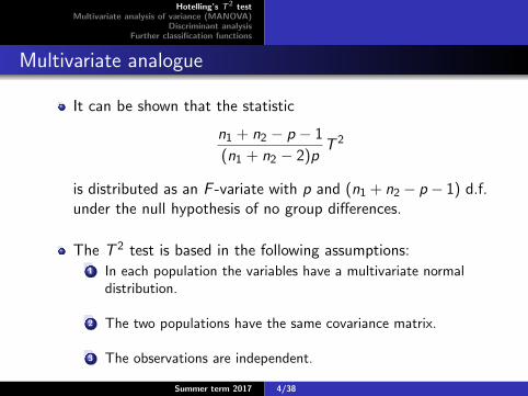
It can be shown that the statistic

n1 + n2 − p − 1

(n1 + n2 − 2)pT 2

is distributed as an F -variate with p and (n1 + n2 − p− 1) d.f.under the null hypothesis of no group differences.

The T 2 test is based in the following assumptions:1 In each population the variables have a multivariate normal

distribution.

2 The two populations have the same covariance matrix.

3 The observations are independent.




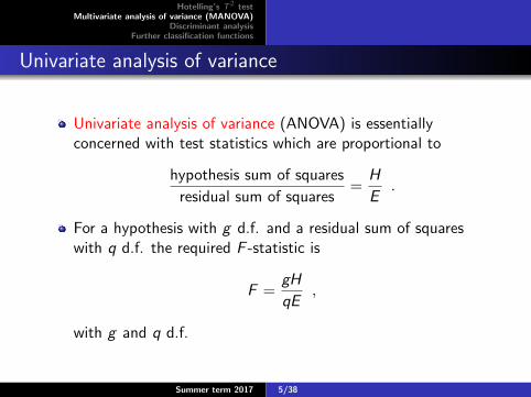
Univariate analysis of variance

Univariate analysis of variance (ANOVA) is essentiallyconcerned with test statistics which are proportional to

hypothesis sum of squares

residual sum of squares=

H

E.

For a hypothesis with g d.f. and a residual sum of squareswith q d.f. the required F -statistic is

F =gH

qE,

with g and q d.f.





Multivariate analysis of variance (MANOVA) is based on thehypothesis sums of squares and cross-products matrix (H) andan error matrix (E), the elements of which are defined asfollows:

hrs =m∑i=1

ni (xir − xr )(xis − xs) , r , s = 1, . . . , p ,

ers =m∑i=1

ni∑j=1

(xijr − xir )(xijs − xis) , r , s = 1, . . . , p ,

where xir is the mean of variable r in group i with sample sizeni (i = 1, . . . ,m), and xr is the grand mean of variable r .




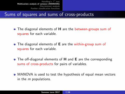
Sums of squares and sums of cross-products

The diagonal elements of H are the between-groups sum ofsquares for each variable.

The diagonal elements of E are the within-group sum ofsquares for each variable.

The off-diagonal elements of H and E are the correspondingsums of cross-products for pairs of variables.

MANOVA is used to test the hypothesis of equal mean vectorsin the m populations.




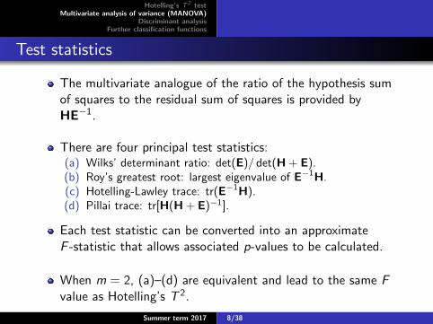
Test statistics

The multivariate analogue of the ratio of the hypothesis sumof squares to the residual sum of squares is provided byHE−1.

There are four principal test statistics:(a) Wilks’ determinant ratio: det(E)/ det(H + E).(b) Roy’s greatest root: largest eigenvalue of E−1H.(c) Hotelling-Lawley trace: tr(E−1H).(d) Pillai trace: tr[H(H + E)−1].

Each test statistic can be converted into an approximateF -statistic that allows associated p-values to be calculated.

When m = 2, (a)–(d) are equivalent and lead to the same Fvalue as Hotelling’s T 2.




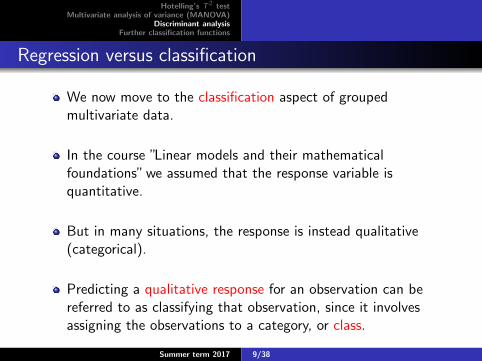
Regression versus classification

We now move to the classification aspect of groupedmultivariate data.

In the course ”Linear models and their mathematicalfoundations” we assumed that the response variable isquantitative.

But in many situations, the response is instead qualitative(categorical).

Predicting a qualitative response for an observation can bereferred to as classifying that observation, since it involvesassigning the observations to a category, or class.




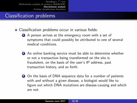
Classification problems

Classification problems occur in various fields:1 A person arrives at the emergency room with a set of

symptoms that could possibly be attributed to one of severalmedical conditions.

2 An online banking service must be able to determine whetheror not a transaction being transformed on the site isfraudulent, on the basis of the user’s IP address, pasttransaction history, and so forth.

3 On the basis of DNA sequence data for a number of patientswith and without a given disease, a biologist would like tofigure out which DNA mutations are disease-causing and whichare not.




Classification setting

Just as in regression, in the classification setting we have a setof training observations (xi , yi ) for i = 1, . . . , n that we canuse to build a classifier.

We want our classifier to perform well not only on the trainingdata, but also on the test observations that were not used totrain the classifier.

In this lecture, we discuss three of the most widely usedclassifiers: discriminant analysis, K -nearest neighbours, andlogistic regression.

More computer-intensive methods such as decision trees willbe discussed in later lectures.




Using Bayes’ theorem for classification

Suppose that we wish to classify an observation into one ofK ≥ 2 classes.

Bayes’ theorem states that

P(Y = k|X = x) =πk fk(x)∑Kl=1 πl fl(x)

,

where πk denotes the prior probability that a randomly chosenobservation is associated with the kth category of the responsevariable Y (k = 1, . . . ,K ) and fk(x) is the density function ofX for an observation that comes from the kth class.

We refer to P(Y = k|X = x) as the posterior probability thatan observation belongs to the kth class, given the predictorvalue for that observation.




Bayes classifier

The Bayes classifier classifies an observation to the class forwhich the posterior probability P(Y = k|X = x) is largest.

It has lowest possible test error rate out of all classifiers.

The Bayes error rate at X = x0 is 1−maxk P(Y = k|X = x0).In general, the overall Bayes error rate is

1− E

(maxk

P(Y = k|X )

),

where the expectation averages the probability over allpossible values of X .

If we can find a way to estimate fk(x), then we can develop aclassifier that approximates the Bayes classifier.




Linear discriminant analysis with one predictor

For now, assume that p = 1, that is, we have only onepredictor.

We would like to obtain an estimate for fk(x) that we canplug into the Bayes’ theorem in order to estimatepk(x) = P(Y = k|X = x).

We will then classify an observation to the class for whichpk(x) is greatest.

In order to estimate fk(x), we will first make someassumptions about its form.




Linear discriminant analysis with one predictor (2)

Suppose we assume that fk(x) is Gaussian. In theone-dimensional setting, the normal density takes the form

fk(x) =1√

2πσkexp

(− 1

2σ2k

(x − µk)2

),

where µk and σ2k are the mean and variance for the kth class.

For now, let us further assume that σ21 = · · · = σ2

K .

That is, there is a shared variance across all K classes, whichwe denote by σ2.





Plugging this form of fk(x) into Bayes’ theorem, we find that

pk(x) =πk

1√2πσ

exp(− 1

2σ2 (x − µk)2)

∑Kl=1 πl

1√2πσ

exp(− 1

2σ2 (x − µl)2) .

We then assign the observation to the class for which

δk(x) = xµkσ2− µ2

k

2σ2+ ln(πk)

is largest.





For instance, if K = 2 and π1 = π2, then the Bayes classifierassigns an observation to class 1 if

2x(µ1 − µ2) > µ21 − µ2

2 ,

and to class 2 otherwise.

In this case, the Bayes decision boundary corresponds to thepoint where

x =µ2

1 − µ22

2(µ1 − µ2)=µ1 + µ2

2.





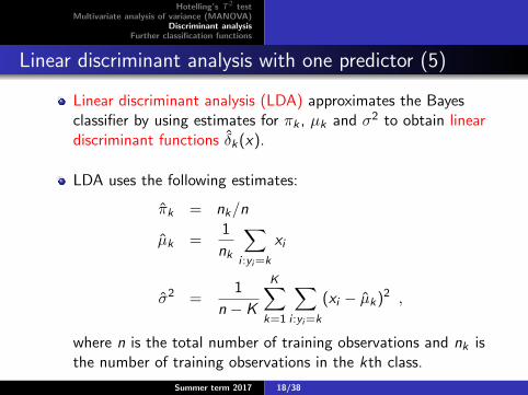
Linear discriminant analysis (LDA) approximates the Bayesclassifier by using estimates for πk , µk and σ2 to obtain lineardiscriminant functions δk(x).

LDA uses the following estimates:

πk = nk/n

µk =1

nk

∑i :yi=k

xi

σ2 =1

n − K

K∑k=1

∑i :yi=k

(xi − µk)2 ,

where n is the total number of training observations and nk isthe number of training observations in the kth class.




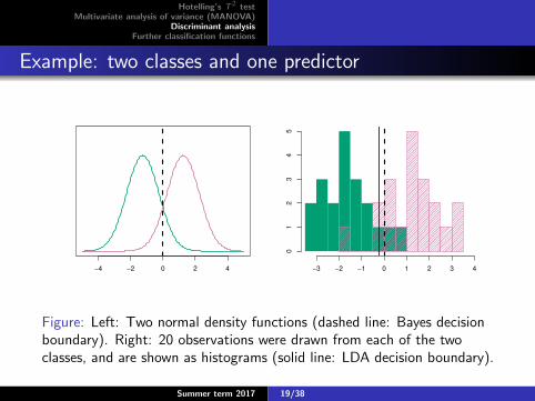
Example: two classes and one predictor

−4 −2 0 2 4 −3 −2 −1 0 1 2 3 4

01

23

45

Figure: Left: Two normal density functions (dashed line: Bayes decisionboundary). Right: 20 observations were drawn from each of the twoclasses, and are shown as histograms (solid line: LDA decision boundary).




Linear discriminant analysis with multiple predictors

To extend the LDA classifier to the case p > 1, we willassume that x = (x1, . . . , xp)> is drawn from a multivariatenormal distribution, with E(x) = µ, Cov(x) = Σ and density

f (x) =1

(2π)p/2 det(Σ)1/2exp

(−1

2(x− µ)>Σ−1(x− µ)

).

LDA assumes that the observations in the kth class are drawnfrom Nk(µk ,Σ).

We assign an observation x to the class for which

δk(x) = x>Σ−1µk −1

2µ>k Σ−1µk + ln(πk)

is largest. To apply LDA, we need estimates of µk , πk and Σto obtain δk(x).




Example: three classes and two predictors

−4 −2 0 2 4

−4

−2

02

4

−4 −2 0 2 4

−4

−2

02

4

X1X1

X2

X2

Figure: Left: ellipses that contain 95% of the probability for each of thethree classes are shown (dashed lines: Bayes decision boundaries). Right:20 observations were generated from each class (solid lines: LDA decisionboundaries).




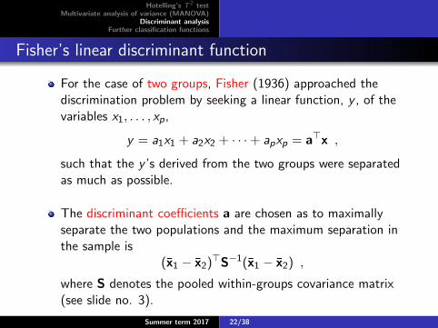
Fisher’s linear discriminant function

For the case of two groups, Fisher (1936) approached thediscrimination problem by seeking a linear function, y , of thevariables x1, . . . , xp,

y = a1x1 + a2x2 + · · ·+ apxp = a>x ,

such that the y ’s derived from the two groups were separatedas much as possible.

The discriminant coefficients a are chosen as to maximallyseparate the two populations and the maximum separation inthe sample is

(x1 − x2)>S−1(x1 − x2) ,

where S denotes the pooled within-groups covariance matrix(see slide no. 3).




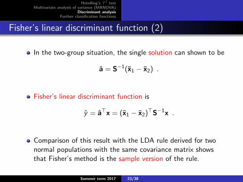
Fisher’s linear discriminant function (2)

In the two-group situation, the single solution can shown to be

a = S−1(x1 − x2) .

Fisher’s linear discriminant function is

y = a>x = (x1 − x2)>S−1x .

Comparison of this result with the LDA rule derived for twonormal populations with the same covariance matrix showsthat Fisher’s method is the sample version of the rule.




Allocation rule based on Fisher’s discriminant function

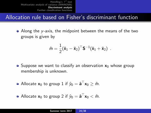
Along the y -axis, the midpoint between the means of the twogroups is given by

m =1

2(x1 − x2)>S−1(x1 + x2) .

Suppose we want to classify an observation x0 whose groupmembership is unknown.

Allocate x0 to group 1 if y0 = a>x0 ≥ m.

Allocate x0 to group 2 if y0 = a>x0 < m.




Confusion matrix and performance measures

148 4. Classification

ROC Curve

False positive rate

True

pos

itive

rat

e

0.0 0.2 0.4 0.6 0.8 1.0

0.0

0.2

0.4

0.6

0.8

1.0

FIGURE 4.8. A ROC curve for the LDA classifier on the Default data. Ittraces out two types of error as we vary the threshold value for the posteriorprobability of default. The actual thresholds are not shown. The true positive rateis the sensitivity: the fraction of defaulters that are correctly identified, usinga given threshold value. The false positive rate is 1-specificity: the fraction ofnon-defaulters that we classify incorrectly as defaulters, using that same thresholdvalue. The ideal ROC curve hugs the top left corner, indicating a high true positiverate and a low false positive rate. The dotted line represents the “no information”classifier; this is what we would expect if student status and credit card balanceare not associated with probability of default.

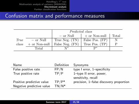
Predicted class− or Null + or Non-null Total

True − or Null True Neg. (TN) False Pos. (FP) Nclass + or Non-null False Neg. (FN) True Pos. (TP) P

Total N∗ P∗

TABLE 4.6. Possible results when applying a classifier or diagnostic test to apopulation.

minus the specificity of our classifier. Since there is an almost bewilderingspecificity

array of terms used in this context, we now give a summary. Table 4.6shows the possible results when applying a classifier (or diagnostic test)to a population. To make the connection with the epidemiology literature,we think of “+” as the “disease” that we are trying to detect, and “−” asthe “non-disease” state. To make the connection to the classical hypothesistesting literature, we think of “−” as the null hypothesis and “+” as thealternative (non-null) hypothesis. In the context of the Default data, “+”indicates an individual who defaults, and “−” indicates one who does not.

Name Definition Synonyms

False positive rate FP/N type I error, 1–specificityTrue positive rate TP/P 1–type II error, power,

sensitivity, recallPositive predictive value TP/P* precision, 1–false discovery proportionNegative predictive value TN/N*




Receiver operating characteristics (ROC) curveROC Curve

False positive rate

Tru

e p

ositiv

e r

ate

0.0 0.2 0.4 0.6 0.8 1.0

0.0

0.2

0.4

0.6

0.8

1.0

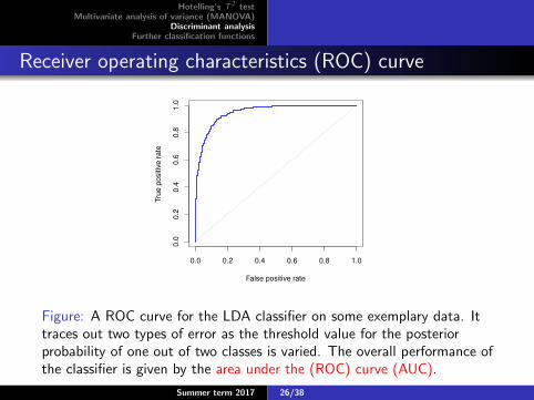
Figure: A ROC curve for the LDA classifier on some exemplary data. Ittraces out two types of error as the threshold value for the posteriorprobability of one out of two classes is varied. The overall performance ofthe classifier is given by the area under the (ROC) curve (AUC).




Quadratic discriminant analysis

Quadratic discriminant analysis (QDA) assumes than anobservation from the kth class is of the form Nk(µk ,Σk).

Under this assumption, we assign an observation x to the classfor which

δk(x) = −1

2(x−µk)>Σ−1(x−µk)− 1

2ln(det(Σk)) + ln(πk) .

is largest.

QDA involves plugging estimates for Σk , µk and πk to obtainthe quadratic discrimination function δk(x).




Quadratic discriminant analysis (2)

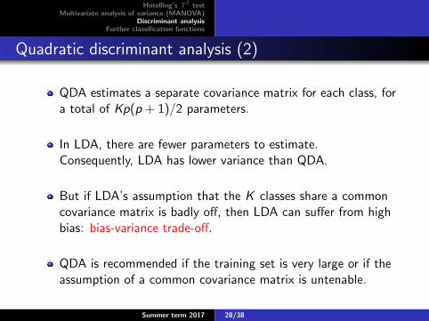
QDA estimates a separate covariance matrix for each class, fora total of Kp(p + 1)/2 parameters.

In LDA, there are fewer parameters to estimate.Consequently, LDA has lower variance than QDA.

But if LDA’s assumption that the K classes share a commoncovariance matrix is badly off, then LDA can suffer from highbias: bias-variance trade-off.

QDA is recommended if the training set is very large or if theassumption of a common covariance matrix is untenable.




Quadratic discriminant analysis (3)

−4 −2 0 2 4

−4

−3

−2

−1

01

2

−4 −2 0 2 4

−4

−3

−2

−1

01

2

X1X1

X2

X2

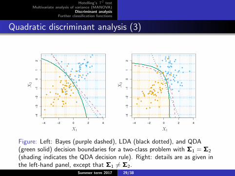
Figure: Left: Bayes (purple dashed), LDA (black dotted), and QDA(green solid) decision boundaries for a two-class problem with Σ1 = Σ2

(shading indicates the QDA decision rule). Right: details are as given inthe left-hand panel, except that Σ1 6= Σ2.




K -nearest neighboursLogistic regression

The KNN approach

The K -nearest neighbour (KNN) classification approach is anon-parametric method.

Given a positive integer K and a test observation x0, the KNNclassifier first identifies the K observation in the training datathat are closest to x0, represented by M0.

It then estimates

P(Y = k|X = x0) =1

K

∑i∈M0

I (yi = k) ,

where I (·) denotes the indicator function.

Finally, KNN classifies x0 to the class with the highestestimated probability (known as majority vote).





Illustrative example of the KNN approach

o

o

o

o

o

oo

o

o

o

o

o o

o

o

o

o

oo

o

o

o

o

o

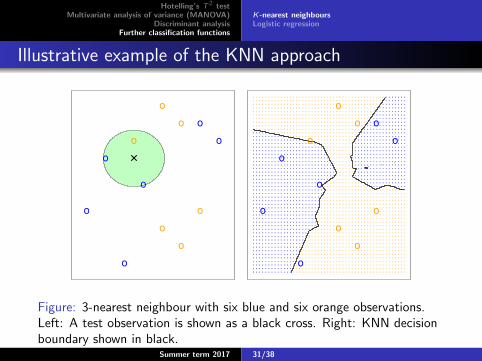
Figure: 3-nearest neighbour with six blue and six orange observations.Left: A test observation is shown as a black cross. Right: KNN decisionboundary shown in black.





The choice of K in KNN

The choice of K can have a drastic effect on the performanceof the KNN classifier.

As K grows, the method becomes less flexible. Thiscorresponds to a low-variance but high-bias classifier.

KNN can be viewed as assigning the K nearest neighbours aweight 1/K and all others zero weight.

When K = 1, the KNN training error rate is zero, but the testerror rate may be quite high.





KNN training and test error rate

0.01 0.02 0.05 0.10 0.20 0.50 1.00

0.0

00

.05

0.1

00

.15

0.2

0

1/K

Err

or

Ra

te

Training Errors

Test Errors

Figure: KNN training and test error rate on some data as 1/K increases.





The logistic model

Logistic regression models the probability that the responsebelongs to a particular category.

Consider a binary response (0/1) and a single predictor. Thesigmoid logistic function ensures that p(x) = P(Y = 1|X ) liesbetween 0 and 1:

p(x) =exp(β0 + β1x)

1 + exp(β0 + β1x).

The logit (log-odds) is linear in the predictor:

ln

(p(x)

1− p(x)

)= β0 + β1x .





Fitting the model and making predictions

The coefficients β0 and β1 are unknown and must beestimated based on the available training data.

Various methods for fitting the model are available (e.g.maximum likelihood).

In logistic regression, increasing X by one unit, multiplies theodds by exp(β1) or changes the log-odds by β1.

Once the regression coefficients have been estimated, we canpredict the probability p(x) as follows:

p(x) =exp(β0 + β1x)

1 + exp(β0 + β1x).





Multiple logistic regression

Simple logistic regression easily generalizes to multiple logisticregression with more than one predictor:

ln

(p(x)

1− p(x)

)= β0 + β1x1 + · · ·+ βpxp .

where x1, . . . , xp are p predictors.

The probability p(x) turns into

p(x) =exp(β0 + β1x1 + · · ·+ βpxp)

1 + exp(β0 + β1x1 + · · ·+ βpxp).

When there is correlation among the predictors, then thisphenomenon is known as collinearity.





Logistic regression for more than two response classes

We sometimes wish to classify a response variable that hasmore than two classes.

Multinomial logistic regression is a classification method thatgeneralizes logistic regression to multi-class problems.

Multinomial logistic regression is used when the dependentvariable in question is nominal.

The ordered logit model, also called ordered logistic regression,is a regression model for ordinal dependent variables.





Comparison of classification methods

Both logistic regression and LDA produce linear decisionboundaries and only differ in their fitting procedures.

KNN does not make any assumptions about the shape of thedecision boundary; we can expect it to perform well when thedecision boundary is highly non-linear.

QDA serves as a compromise between the KNN method andthe linear methods; it assumes a quadratic decision boundaryand can accurately model a wider range of problems than canthe linear models.

Some of the figures in this presentation are taken from “An Introduction to StatisticalLearning, with applications in R” (Springer, 2013) with permission from the authors:G. James, D. Witten, T. Hastie and R. Tibshirani.
