Multiple-Criteria Optimization of a Cold Heading Process using Finite Element Analysis and a
Taguchi Approach
by
Christine EI-Lahham
Department of Mechanical Engineering McGill University Montreal, Canada
A Thesis submitted to McGill University in partial fulfillment of the requirements for the degree of
Master of Engineering
Under the supervision of: Professor J.A. Nemes
McGill University
© Christine EI-Lahham October, 2003

1+1 Library and Archives Canada
Bibliothèque et Archives Canada
Published Heritage Branch
Direction du Patrimoine de l'édition
395 Wellington Street Ottawa ON K1A ON4 Canada
395, rue Wellington Ottawa ON K1A ON4 Canada
NOTICE: The author has granted a nonexclusive license allowing Library and Archives Canada to reproduce, publish, archive, preserve, conserve, communicate to the public by telecommunication or on the Internet, loan, distribute and sell th es es worldwide, for commercial or noncommercial purposes, in microform, paper, electronic and/or any other formats.
The author retains copyright ownership and moral rights in this thesis. Neither the thesis nor substantial extracts from it may be printed or otherwise reproduced without the author's permission.
ln compliance with the Canadian Privacy Act some supporting forms may have been removed from this thesis.
While these forms may be included in the document page count, their removal does not represent any loss of content from the thesis.
• •• Canada
AVIS:
Your file Votre référence ISBN: 0-612-98523-7 Our file Notre référence ISBN: 0-612-98523-7
L'auteur a accordé une licence non exclusive permettant à la Bibliothèque et Archives Canada de reproduire, publier, archiver, sauvegarder, conserver, transmettre au public par télécommunication ou par l'Internet, prêter, distribuer et vendre des thèses partout dans le monde, à des fins commerciales ou autres, sur support microforme, papier, électronique et/ou autres formats.
L'auteur conserve la propriété du droit d'auteur et des droits moraux qui protège cette thèse. Ni la thèse ni des extraits substantiels de celle-ci ne doivent être imprimés ou autrement reproduits sans son autorisation.
Conformément à la loi canadienne sur la protection de la vie privée, quelques formulaires secondaires ont été enlevés de cette thèse.
Bien que ces formulaires aient inclus dans la pagination, il n'y aura aucun contenu manquant.
Abstract
The current work aims at modeling a three-stage cold heading process of an industrial
boIt, and presents a methodology for the optimization of preform die geometries.
The process is modeled using finite element simulations and potential defects in the
heading process are analyzed using external and internaI crack criteria. The preform
geometries are then optimized with respect to external cracking in the blank and forming
die load. The conventional Taguchi approach is first applied on each criterion separately.
Three optimal solutions are generated. It is found that sorne parameters have conflicting
optimal solutions.
The single criterion approach is therefore extended to multiple-criteria approaches by the
use of overall evaluation criteria within the Taguchi method. Two methodologies are
proposed, namely, the additive utility function method and the TOPSIS decision-making
mode!. It is found that the performances of the two methods are comparable.
1
Résumé
Le présent travail vise à modéliser un processus à trois étapes de formage à froid d'un
boulon industriel, et présente une méthodologie permettant d'optimiser la géométrie des
matrices servant à la préforme.
Le processus est modélisé numériquement par la méthode de simulation des éléments
finis. Les défauts potentielles de ce processus de formage sont analysés par des critères
de fissuration internes et externes. La géométrie des matrices servant à la préforme est
alors optimisée en considérant la fissuration externe des boulons ainsi que la charge
externe des matrices. L'approche conventionnelle de Taguchi est d'abord appliquée sur
chaque critère séparément permettant d'obtenir trois solutions optimales. Les résultats
obtenus indiquent que certains paramètres ont des solutions optimales contradictoires.
L'approche d'un seul critère est donc remplacé par des approches à critères multiples en
utilisant 'un critère d'évaluation globale' au sein de la méthode de Taguchi. Deux
méthodologies sont alors proposées, la méthode de fonction utilitaire additive et le
modèle de prise de décision TOPSIS. On constate que les performances de ces deux
méthodes sont comparables.
II

Acknowledgements
1 would like to first thank my supervisor, Professor James A. Nemes, for his guidance and
encouragement.
The supporters of this project are also greatly acknowledged: the Natural Sciences and
Engineering Research Council of Canada (NSERC), Le Fonds Quebecois de Recherche
sur la Nature et les Technologies (FQRNT) and Ivaco Rolling Mills.
For his advice and invaluable insight for this work, 1 would like to thank my colleague,
Abbas S. Milani.
Finally, 1 thank my family and friends for their love and support.
III
Table of Contents
Abstract
Résumé
A cknowledgements
Table of contents
List of Figures
List of Tables
1. INTRODUCTION
1.1 Literature Review 1.1.1 Simulation of the cold heading process 1.1.2 Ductile fracture criteria 1.1.3 Optimization techniques for fonning processes
1.1.3.1 Single criterion approach 1.1.3.2 Multiple criteria approach
2. MATHEMATICAL BACKGROUND
2.1 Constitutive Equation
2.2 Failure Criteria 2.2.1 External Cracks 2.2.2 InternaI Cracks
2.2.2.1 Initiation of localization 2.2.2.2 Defonnation adiabatic shear band fonnation (DASB) 2.2.2.3 Transfonnation adiabatic shear band fonnation (TASB)
2.3 The Taguchi Approach 2.3.1 Design of Experiments 2.3.2 Producing an optimum solution 2.3.3 The predictive equation and verification of additivity 2.3.4 ANOY A analysis on Taguchi results
2.4 Multiple-Criteria Optimization 2.4.1 The MODM approach
2.4.1.1 The utility function method 2.4.2 The MADM approach
2.4.2.1 Solution method (TOP SIS)
IY
1
II
III
IV
VI
IX
1
2 2 6 8 8
10
12
12
14 14 16 16 17 19
20 20 21 23 24
25 27 27 29 30
3. NUMERICAL ANAL YSIS
3.1 Description of Simulation
3.2 Assessment of Potential Defects 3.2.1 External Cracking 3.2.2 InternaI Cracking 3.2.3 Analysis of a harder steel
3.3 Summary
4. SINGLE CRITERIA OPTIMIZATION
4.1 Experiments: the L-9 Orthogonal Array
4.2 Convention al Taguchi Optimization 4.2.1 Factor Plots 4.2.2 Additivity of the method 4.2.3 ANOV A Analysis
4.3 Discussion
5. MULTIPLE CRITERIA OPTIMIZATION
5.1 Selected Methods
34
34
40 40 41 44 47
48
50
55 55 56 57
57
61
62
5.2 Utility Function Methods 62 5.2.1 Weight 5 as an illustrative example 64 5.2.2 Sensitivity to changes in weights and breakdown point 68 5.2.3 Compatibility with single criterion optimization 68 5.2.4 Extent ofparameter level differentiation 69 5.2.5 Pareto frontiers 70
5.3 A new OEC approach within the Taguchi method: TOPSIS 71 5.3.1 The TOPSIS method compared to the additive utility function method 73
5.4 Sensitivity to outlier points 78
6. CONCLUSIONS AND FUTURE WORK 79
REFERENCE LIST 82
v
List of Figures
FIGURE 1-1: SCHEMATIC OF A FOUR-STATION BOLT-MAKlNG MACHINE ............................. 3
FIGURE 1-2: THREE BASIC RULES FOR UPSET FORGING ....................................................... 4
FIGURE 1-3: ALLOWABLE LIMITS IN UPSETTING ................................................................. 5
FIGURE 1-4: DESIGN PARAMETERS IN COINING STAGES ..................................................... 8
FIGURE 2-1 : TEST SPECIMEN BETWEEN UPPER AND LOWER DIES ...................................... 15
FIGURE 2-2: ONS ET OF LONGITUDINAL CRACKING ON HEAD SURFACE ............................ 15
FIGURE 2-3: INTERNAL CRACK RESUL TING FROM SHEAR LOCALIZATION ......................... 17
FIGURE 2-4: DEFORMATION ADIABATIC SHEAR BAND CRITERION .................................... 18
FIGURE 2-5: A TRANSFORMATION SHEAR BAND .............................................................. 19
FIGURE 2-6: A REPRESENTATION OF AN MADM DECISION MA TRIX ............................... 34
FIGURE 3-1: THE COMMON BOLT THAT IS MODELED ......................................................... 37
FIGURE 3-2: SCHEMATIC OF A THREE-STAGE COLD HEADING PROCESS ............................. 37
FIGURE 3-3: COLD HEADING SIMULATION STEPS ............................................................... 37
FIGURE 3-4: TEMPERATURE CHANGE FOR TWO THICKNESSES WITHIN THE DEFORMED
BLANK, DURING UNLOADING STAGES .................................................................................. 38
FIGURE 3-5: SCHEMATIC OF THE FINITE ELEMENT MODEL. ................................................. 38
FIGURE 3-6: TENSILE TEST CURVE FITTING FOR DETERMINATION OF JOHNSON-COOK
P ARAMETERS ....................................................................................................................... 39
FIGURE 3-7: EVOLUTION OF PLASTIC STRAIN IN THE BLANK ............................................. 39
FIGURE 3-8: (A) MAXIMUM PRINCIPAL STRESS AND (B) TEMPERATURE CONTOURS .......... 40
FIGURE 3-9: C PARAMETER AS A FUNCTION OF STRAIN ON THE EXTERIOR SURFACE OF
THE BLANK .......................................................................................................................... 42
FIGURE 3-10: EVOLUTION OF HARDENING AND SOFTENING TERMS, INDICA TING ONSET
OF LOCALIZATION ............................................................................................................... 43
VI
FIGURE 3-11 : EQUIVALENT STRESS VS. EQUIVALENT STRAIN FOR AN ELEMENT WITHIN
THE BAND ............................................................................................................................ 43
FIGURE 3-12: MICROSTRUCTURE OF 1008 STEEL IN (A) AS-ROLLED STATE (B) HIGHLY
DEFORMED STATE ................................................................................................................ 44
FIGURE 3-13: C PARAMETER AS A FUNCTION OF STRAIN ON THE EXTERIOR SURFACE OF A
1038 BLANK ........................................................................................................................ 45
FIGURE 3-14: EVOLUTION OF HARDENING AND SOFTENING TERMS, INDICA TING ONSET OF
LOCALIZATION .................................................................................................................... 45
FIGURE 3-15 : EQUIVALENT STRESS vs. EQUIVALENT STRAIN FOR AN ELEMENT WITHIN
THE BAND ............................................................................................................................ 46
FIGURE 3-16: TEMPERA TURE VS. EQUIVALENT STRAIN FOR AN ELEMENT WITHIN THE
BAND .................................................................................................................................. 46
FIGURE 4-1 : SCHEMA TIC OF THE FOUR DESIGN PARAMETERS .......................................... .49
FIGURE 4-2: UPSETTING IS PERFORMED IN THE FREE HEADING REGION ............................ 50
FIGURE 4-3: SHEAR BAND INITIATION CRITERION FOR EXPERIMENTS 1,4 AND 7 .............. 52
FIGURE 4-4: DEFORMATION ADIABA TIC SHEAR BAND CRITERION FOR EXPERIMENTS
1,4 AND 7 ............................................................................................................................ 53
FIGURE 4-5: TRANSFORMATION ADIABATIC SHEAR BAND CRITERION FOR EXPERIMENTS
(A) 1, (B) 4 AND (C) 7 ........................................................................................................ 53
FIGURE 4-6: C PARAMETER AS A FUNCTION OF STRAIN FOR AN ELEMENT ON THE
EXTERIOR SURFACE ............................................................................................................. 54
FIGURE 4-7: (A) DIEL LOAD 1 RESPONSE (B) DIE LOAD 2 RESPONSE ................................ 55
FIGURE 4-8: FACTOR-PLOTOFC PARAMETER ................................................................... 59
FIGURE 4-9: FACTOR-PLOTS OF PREFORM DIE LOAD FOR (A) DIE 1 (B) DIE 2 .................... 59
FIGURE 5-1: FACTOR PLOTS FOR WEIGHT 5 (A) UADDITIVE, (B) UMINIMAX,
(C) UMULTIPLICATIVE ......................................................................................................... 67
FIGURE 5-2: PARETO FRONTIERBETWEEN (A) C AND F FOR DIE 1, (B) C AND F
FOR DIE 2 ............................................................................................................................ 71
FIGURE 5-3: (A) GRAPHICAL REPRESENTATION OF TOPSIS SOLUTION AND (B)
COMPARISON WITH THE ADDITIVE METHOD, FOR DESIGN FACTOR A USING WEIGHT 5 ......... 76
VII

FIGURE 5-4: (A) GRAPHICAL REPRESENTATION OF TOPSIS SOLUTION AND (B)
COMPARISON WITH THE ADDITIVE METHOD, FOR DESIGN FACTOR H USING WEIGHT 5 ......... 76
FIGURE 5-5: (A) GRAPHICAL REPRESENTATION OF TOPSIS SOLUTION AND (B)
COMPARISON WITH THE ADDITIVE METHOD, FOR DESIGN FACTOR LI USING WEIGHT 5 ....... 77
FIGURE 5-6: (A) GRAPHICAL REPRESENTATION OF TOPSIS SOLUTION AND (B)
COMPARISON WITH THE ADDITIVE METHOD, FOR DESIGN FACTOR L2 USING WEIGHT 5 ...... 77
VIII
List of Tables
TABLE 2.1: L-9 ORTHOGONAL ARRA y .............................................................................. 21
TABLE 4.1 : FACTORS AND THEIR LEVEL VARIATIONS ......................................................... 52
TABLE 4.2: THE L-9 ORTHOGONALARRAY AND NUMERICALRESPONSE OF EXPERIMENTS.52
TABLE 4.3: AVERAGE RESPONSE FOR EACH PARAMETER LEVEL ........................................ 58
TABLE 4.4: OPTIMAL COMBINATIONS WITH RESPECT TO EACH FACTOR ............................. 59
TABLE 4.5: ADDITIVITY OF THE METHOD USING THE PREDICTIVE EQUATION ..................... 59
TABLE 4.6: ANOV A FOR RESPONSE C .............................................................................. 60
TABLE 4.7: ANOVA FOR RESPONSE DIE LOAD 1 ............................................................... 60
TABLE 4.8: ANOV A FOR RESPONSE DIE LOAD 2 .............................................................. 60
TABLE 5.1: NORMALIZED RESPONSE VALUES IN L-9 ........................................................... 64
TABLE 5.2: WEIGHTS AND OPTIMAL SOLUTIONS FOR DIFFERENT MULTI-CRITERIA
T AGUCHI OPTIMIZATION METHODS ..................................................................................... 64
TABLE 5.3: WEIGHTED NORMALIZED RESPONSE (WEIGHT 5) ............................................. 65
TABLE 5.4: UTILITY FUNCTION VALUES FOR WEIGHT 5 ...................................................... 66
TABLE 5.5: AVERAGERESPONSE FOREACH PARAMETER LEV EL FOR WEIGHT 5 ................. 66
TABLE 5.6: DECISION MATRICES BEFORE NORMALIZATION ................................................ 75
TABLE 5.7: WEIGHTS AND OPTIMAL SOLUTIONS FOR ADDITIVE AND TOPSIS TAGUCHI
OPTIMIZA TION METHODS ..................................................................................................... 75
TABLE 5.8: NORMALIZED DECISION MATRICES AND IDEAL AND NADIR POINTS
(WEIGHT 5) .......................................................................................................................... 75
TABLE 5.9: RESPONSE VALUES OF ADDITIVE AND TOPSIS METHODS FOR WEIGHT 5 ........ 77
TABLE 5.10: CRITERIA VALUES OF EACH METHOD' S NEW OPTIMUM COMBINA TION WITH
AN OUTLIER POINT ............................................................................................................... 78
IX

1. Introduction
The cold heading process (CHP) is an important manufacturing technique that is
commonly used to produce fasteners, such as bolts, rivets, and nuts. In this technique,
parts are brought to near net shape without an extemal heat source, using a pre
determined sequence of blows that result in average strain rates exceeding 100 S-I, and
local rates higher by as much as one or two orders of magnitude.
Even though it is very widely used, the CHP can produce a number of potential defects in
the formed part. These defects, if not causing rejection before going into service, can be
detrimental to a part's life. Tooling costs, which depend on tool wear, are additional
significant cold forging costs (Groenbaek and Birker, 1999).
Recently, therefore, much attention has been given to the design of forming stages. In
particular, the need to produce defect-free parts with minimal die wear has become
extensively linked to the preform geometries. In the past, cold forming design used to
rely on empirical knowledge and the designer's experience. The focus now is on the use
of numerical simulations that can make this process much faster and more efficient.
In this work, finite element simulations are used to model a three-stage co Id heading
process of a common boIt. Different failure criteria are employed to predict internaI and
extemal fracture. Preform geometries, used in the cold heading process, are then
optimized with respect to part failure and forming load using different multiple-criteria
methods. The methodology presented in this work may be useful in the optimization of
various other forming processes.

1.1 Literature Review
1.1.1 Simulation of the co Id heading process
Many researchers have developed numerical models to simulate various parts of forming
operations. Roque and Button (2000) simulated a basic forming process, upsetting, that is
applied in many cold forging sequences. In their work, experiments have been performed
to obtain the stress-strain response, the material flow during the simulated stage, and the
required forming force, aIl to be used as numerical input data.
MacCormack and Monaghan (2002) modeled the forming of a spline shape on the he ad of
a fastener. The process eonsists of three forging blows, termed the 'eoining',
'cheesehead' and final stages. A schematic of a four-station bolt-making machine is
shown in Figure 1-1, which inc1udes the blank eut-off stage. In their simulations, the top
and bottom dies are rigid and the blank is modeled as an elastoplastie material. It is
mentioned that researeh has shown the Coekroft and Latham failure eriterion to be
amongst the best for practieal applications. Therefore, a critical C value is used as a
damage criterion. At the end of each stage, the top die is unloaded and the deformed
blank allowed to relax in order to stabilize residual stresses. The authors state that one of
the fundamental points about modeling this proeess is that the residual stresses within the
workpiece after each station need to be conserved, as they will affect the flow
characteristics of the material due to strain hardening. At the end of the simulations, the
strain, damage and flow patterns in aIl three stages are analyzed.
In this work, it is also mentioned that coining punches are used before the heading station
beeause they enable heading of a length of wire of up to six times the diameter of the
blank material in only two strokes.
2

eut-Off
Station
Coining
Station
Reading Station
Figure 1-1: Schematic of a four-station boit-ma king machine (MacCormack and Monaghan, 2002)1
Naujoks and Fabel (1948) discuss three basic rules goveming die design for upsetting in
one stage, illustrated schematically in Figure 1-2. The rules are described below.
Rule 1: A blank can be upset in one blow with no buckling or flash injuries if the upset
length, 10 , is less than or equal to three times the blank diameter, do.
Rule 2: For a cylindrical die - If 10 is greater than 3do , and the final head diameter dg is
less than 1.5do ' then the completely unsupported length of the blank, I~, should be at
most equal to halfthe upset length, 10.
Rule 3: For a conical (tapered) die - If 10 is greater than 3do , and the final head diameter
dg is less than 1.5do ' then the completely unsupported length of the blank, I~, should be
at most equal to the blank diameter, do.
1 With author's permission
3

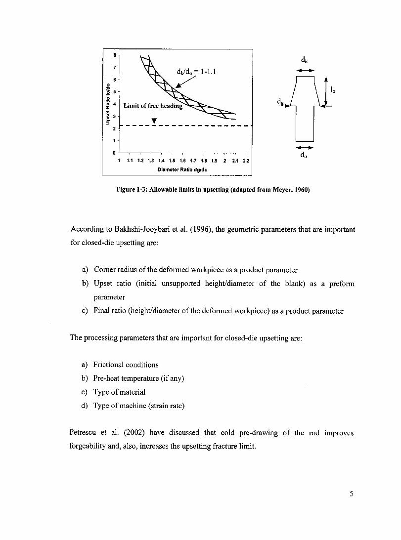
Meyer (1960) provided a relationship between the maximum allowable upset ratio and the
diameter ratio, based on experimental studies, shown in Figure 1-3. This plot provides
certain limits for upsetting. The banded region refers to the set of curves belonging to
ratios, of the preform top diameter to the original blank diameter, varying from 1 to 1.1.
Other ratios are not shown in the plot, however, it is evident from Meyer's results that the
greater the ratio, the lower the limits. It can aiso be noted from Figure 1-3 that the curves
are asymptotic to an upset ratio that is slightly greater than two. Below this upset ratio, a
blank can be headed to any final diameter. This is the free heading region. Going beyond
the banded regions is either infeasible or will produce buckling or other failures.
Gokler et al. (1999) point out that tapered preforms are widely used in multiple-stage
upsetting because they produce well-filled and uniform upsets. This allows greater upset
ratios as compared to cylindrical preforms. They further state that the important design
parameters in taper upsetting, for a given upset ratio (the ratio of unsupported length to
diameter of the initial blank), are the percent reduction in the height of the blank and the
percent increase in the diameter of the head.
Rule 1: 10 ~ 3do
Rule 2: If 10 ~ 3do and dg ~ 1.5do
~l~ ~l;{
Rule 3: If 10 ~ 3do and dg ~ 1.5do
~l~ ~ do
Figure 1-2: Three basic rules for upset forging (adapted from Naujoks and Fabel, 1948)
4
8
7
6 o 'a :g 5
~ ~ 4
~ 3 Il. ::l
2
Limit of free heading .........,~~~
~ ~
1 1.1 1.2 1.3 1.4 1.5 1.6 1.7 1.8 1.9 2 2.1 2.2
Dlameter Ratio dg/do
Figure 1-3: Allowable Iimits in upsetting (adapted from Meyer, 1960)
According to Bakhshi-Jooybari et al. (1996), the geometric parameters that are important
for closed-die upsetting are:
a) Corner radius of the deformed workpiece as a product parameter
b) Upset ratio (initial unsupported heightldiameter of the blank) as a preform
parameter
c) Final ratio (heightldiameter of the deformed workpiece) as a product parameter
The processing parameters that are important for closed-die upsetting are:
a) Frictional conditions
b) Pre-heat temperature (if any)
c) Type of material
d) Type of machine (strain rate)
Petrescu et al. (2002) have discussed that cold pre-drawing of the rod Improves
forgeability and, also, increases the upsetting fracture limit.
5
1.1.2 Ductile fracture criteria
Different damage models are used in the literature, to assess and predict cracks in cold
forming processes. These can be categorized in three parts: macromechanical,
micromechanical, and lately mesomechanical approaches.
Behrens et al. (2000) divide macromechanical damage models into strain-independent
and strain-dependant models. The strain-dependant models are usually integral functions
of stress, strain, and sorne material parameters. Thus they take into account the
deformation history. The strain-independent models do not take into aecount history and
are therefore not suitable for large deformations. Maeromechanieal models, however, are
usually developed for specifie materials or forging operations, which may limit their
application.
Micromechanieal damage criteria describe the effect of stresses at the microstruetural
level when fracture or ductile damage occurs (Behrens et aL, 2000). The criteria consider
that a failure process commences by the creation of miero-cavities that grow to form
defects; the coalescence of the defects at the macro-Ievel eventually causes failure of the
material. These criteria are verified experimentally but their implementation into FE
simulations is still eomplex due to numerical instabilities. Additionally, the necessary
material parameters for these models are difficult to identify.
Mesomechanical models are a new approach, and are the subject of a few recent papers.
Brethenoux et al. (1996), as an example, use a mesoscopic model in their simulations.
This model consists of applying a load to an elementary cell. The elementary cell is
composed of a metallic matrix around an inclusion or second phase, modeled as a rigid
surface. The boundary conditions, imposed on the cell, ensure the periodicity conditions.
Numerical simulations of the complete forming process are used to determine the loading
conditions on the cell. The onset of ductile fracture is defined as the point when voids
grow catastrophically in the radial direction. The obtained results show reasonable
agreement with experimental values.
6
Generally speaking, most researchers still prefer to use the more established
macromechanical approaches. Petrescu et al. (2002) use the well-known Cockroft
Latham criterion and it is found that experimentallocations of fracture corresponded weIl
with areas of highest circumferential stresses. Janicek et al. (2002) studied the influence
of die geometry on the strength and hardening parameters in an open extrusion followed
by heading. Plastic work, similar to the Cockroft-Latham parameter, is used as a fracture
criterion.
In the cold heading process, failures can be classified into two types: external and
internaI. To assess external failures, macromechanical ductile damage criteria as
described above are often used. Typically, these can be expressed mathematically as:
&
Jf(a,e,m)de = C (1. 1)
o
where f is a function of the stress-strain history, mare material parameters and C is the
critical value reached at the onset of fracture.
Less work has been done in assessing internaI failures. It is generally understood that
internaI failure arises from the initiation and formation of shear bands. The initiation of
shear bands is often taken to be the point at which the stress-strain curve at a localized
point starts to drop. Criteria for the formation of shear bands are still not fully developed.
The work of Batra and Kim (1992), consider that a shear band forms when the effective
stress drops to 90% of its peak value under increasing deformation. Deltort (1994)
considered this value to be 80%. The increase in localized temperature due to excessive
plastic work dissipation may also lead to shear band formation. These types of shear
bands have not been addressed greatly in literature.
Recently, experimental results have suggested the coupling of ductile damage models
with viscoplastic models. These models can be applied for internaI failures. In this
approach, the hydrostatic stress is taken into account. The models postulate that plastic
strain initiates damage, which then propagates by the stress triaxiality.
7
1.1.3 Optimization techniques for forming processes
1.1.3.1 Single criterion approach
The approach in the optimization of one or a sequence of stage(s) in a forging process
varies significantly between researchers. The optimization process can involve numerous
criteria to be satisfied and experiments to be performed.
Roy et al. (1997) discuss that in multi-stage forming processes, there are various
parameters that may be either continuo us or discrete in nature. Gradient-based
mathematical optimization techniques that consider continuous variables are therefore
inappropriate for discrete parameters. According to Roy et al. (1997), dynamic
programming, a search technique used for mixed variables, suffers from the problem of
dimensionality and can only handle a small number of design parameters.
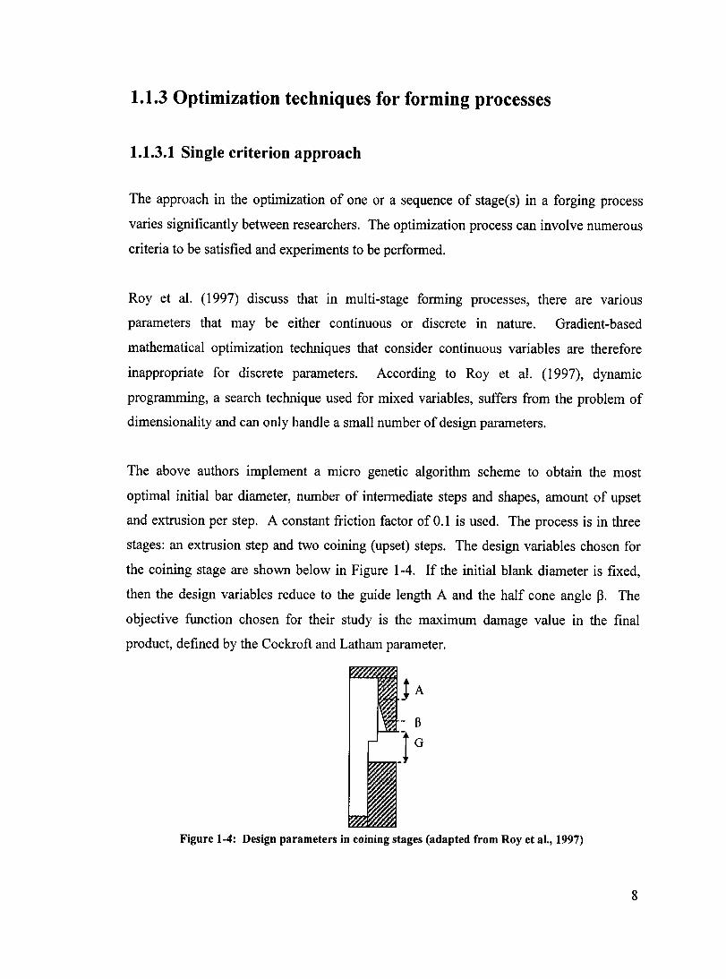
The above authors implement a micro genetic algorithm scheme to obtain the most
optimal initial bar diameter, number of intermediate steps and shapes, amount of upset
and extrusion per step. A constant friction factor of 0.1 is used. The process is in three
stages: an extrusion step and two coining (upset) steps. The design variables chosen for
the coining stage are shown below in Figure 1-4. If the initial blank diameter is fixed,
then the design variables reduce to the guide length A and the half cone angle~. The
objective function chosen for their study is the maximum damage value in the final
product, defined by the Cockroft and Latham parameter.
Figure 1-4: Design parameters in coining stages (adapted from Roy et al., 1997)
8

The Taguchi method has also been widely used in manufacturing to arrive at an optimum
solution. Hwang et al. (2001) summarize the Taguchi method as follows: quality
characteristics (target values of the response) are the objective functions to be optimized.
The objective function is defined by a quadratic loss function. The design variables are
control factors, and the tolerances of design and manufacturing processes are noise
factors. Orthogonal arrays are used to reduce a large number of decisions to a small
number of experiments. The matrix experiments are conducted, the experimental results
are analyzed with respect to the defined loss function and the optimum levels for the
control factors are determined.
Hwang et al. (2001) optimize the design of an automobile outside rearview mirror system.
ln their research, the signal-to-noise ratio in the Taguchi method is replaced by an
objective function of the mean and standard deviations of the quality characteristics,
which includes weighting coefficients for the mean and standard deviations. The number
of design variables is reduced by ANOV A, which is essentially a study of the sensitivity
of the objective function to the variables. The additivity condition of the Taguchi method
is also verified. The finite element method is used to evaluate the vibration behavior
numerically.
Ko et al. (1999) use the Taguchi method to train an artificial neural network (ANN)
model, and finally minimize objective functions relevant to cold heading. The authors
take into consideration two objective functions to be minimized. The first is a damage
parameter, for which they use the criterion suggested by Oh et al. (1979), which differs
from the Cockroft-Latham criterion in that the maximum principle stress is normalized by
the effective stress. The second is the forming load, since properly designed preforming
operations can reduce the load and thus reduce die failure and wear. The design
parameters chosen are guide length and cone angle.
The above authors use an L-9 orthogonal array with two sources of error: friction and
preform die filling. Each error has two levels, aIl experiments are performed and SIN
ratios are generated. This data is then fed into the ANN as train data. The ANN then
9
produces SIN ratios of several other combinations. Two optimal combinations are
produced, one for each objective. The optimal results from the ANN method are very
close to those produced by the Taguchi search method. The authors do not use a multi
objective approach to decide on a final optimum solution. Instead, their work
demonstrates the applicability of the developed ANN method and, additionally, the power
of the Taguchi search method to produce similar results to the seemingly more complex
ANN methods.
1.1.3.2 Multiple criteria approach
When more than one response are to be optimized, different design criteria typically
pro duce considerable conflicts in the choice of optimal parameters. The requirement to
address multiple criteria has prompted sorne researchers to extend single optimization
methods, like the conventional Taguchi method. To date, no unified approach for this has
been suggested, but researchers are examining different methods depending on the
particular application.
Tong and Su (1997) use the TOPSIS CL + value as an index to optimize two responses in
a plasma-enhanced chemical vapor-deposition-process experiment, namely, refractive
index and deposition thickness. They use this index in the Taguchi search method to
obtain an optimal solution. A fuzzy number is initially applied to determine the weight
for each response. The authors perform a cri tic al literature review in multiple-response
optimization.
Kunjur and Krishnamurty (1997) introduced a multi-objective methodology within the
Taguchi method that additionally allows a constrained optimization space. In their work,
a beam design problem is used to illustrate the method. It consists of using ANOV A
results to determine the most significant levels of factors on the objective functions; and
any chosen levels must satisfy the constraints, otherwise they would be rejected. The
final Pareto-optimal solution set depends on the eut-off value that quantifies 'significant',
10

specified by the designer. This method may be comparable to the weighted multi
objective approaches such as the additive or multiplicative methods.
lm (1999) applied artificial intelligence (AI) search techniques to replace knowledge-or
rule-based expert systems, in order to obtain optimal forming sequences for an
axisymmetric pin. In his work, the level of forming 10ad and the effective strain
distributions at each forming stage were subjected for multiple response optimization in
A * and depth-first searches (two AI techniques). The resulting optimized process
sequence is verified numerically and experimentally.
Finally, it can be mentioned that all the above work consider uniform likelihood of
experiments. Otto and Antonsson (1993) extend the Taguchi method by incorporating
different types of uncertainty in the optimization process.
Il
2. Mathematical Background
The mathematical background in this chapter is presented in two main parts. The first
part describes the constitutive equation and the failure criteria proposed for this work. In
the second part, the Taguchi optimization approach is briefly reviewed, followed by a
description of the two multiple-criteria optimization techniques that will be used in
subsequent chapters.
2.1 Constitutive Equation
In the current work, the material is considered to be an elastic-rate-dependant-plastic solid
where the flow stress is given by the empirically based Johnson-Cook expression as
follows:
(2.1)
where A is the yield strength in quasi-static conditions, Band C are material constants and
• n is the work-hardening exponent. The effective plastic strain rate is given by & which is
normalized by ;0 , typically taken to be 1 S-I. T is the current temperature due to plastic
deformation, Ta is the reference temperature, and Tmell is typically the solidus temperature
of the metal.
Therefore the Johnson-Cook model considers the flow stress to be a function of strain,
strain rate and temperature. Each of these is incorporated into the formulation as an
independent term, allowing an uncoupled identification of the corresponding constants.
The model assumes that the strength is isotropie and independent of mean stress.
12
The values of A, B, and n are usually determined by performing quasi-static tension tests
on samples of the material, at room temperature. A can be found directly from the stress
strain data as it is the yield stress. Band n can then be found by re-writing (2.1) as:
In(O" - A) = InB + n In(l') (2.2)
The plot of In(O" - A) verses In(l') is linear, with slope n and intercept InB.
Altematively, the parameters can be determined directly from (2.1) by a non-linear
regression analysis.
To determine C, high-strain rate experiments have to be performed (such as Hopkinson
bar tests). These tests produce stress versus strain data at high strain rates. By
considering one strain, C can then be determined from (2.1) by substituting the values of
the previously determined A,B and n constants and ca1culating the temperature term as
follows. The constant m has been determined experimentally in the literature and is found
to be equal to 1 for a wide range of metals (Johnson and Cook, 1983). The temperature,
T, at each stage of deformation can be found by assuming that most of the plastic work
done transforms into heat in the deforming material. This can be expressed as:
(2.3)
where p is the mass density, Cv is the specifie heat and fJ is the Taylor-Quinney
constant that equals the fraction of the plastic work converted to heat (usually taken to be
~O.9).
13
2.2 Failure Criteria
2.2.1 External Cracks
In the CUITent work, the criterion used for external crack fonnation is the well-known
Cockroft and Latham criterion (Cockroft and Latham, 1968), shown to have considerable
versatility in predicting failure over a wide range of conditions.
The criterion states that fracture occurs when the work done by the maximum tensile
stress attains a critical energy density value 'C'. In general, 'C' can be taken to be a
function of strain rate and temperature. In this work, however, it is considered to be a
constant, which is detennined under conditions approximating those encountered during
the co Id heading process. The criterion can be expressed as:
(2.4)
where 0'/ is the maximum tensile principal stress, & p is the equivalent plastic strain, &1
is the equivalent strain at failure, fJ is the time at failure and the superimposed dot
represents ordinary differentiation with respect to time.
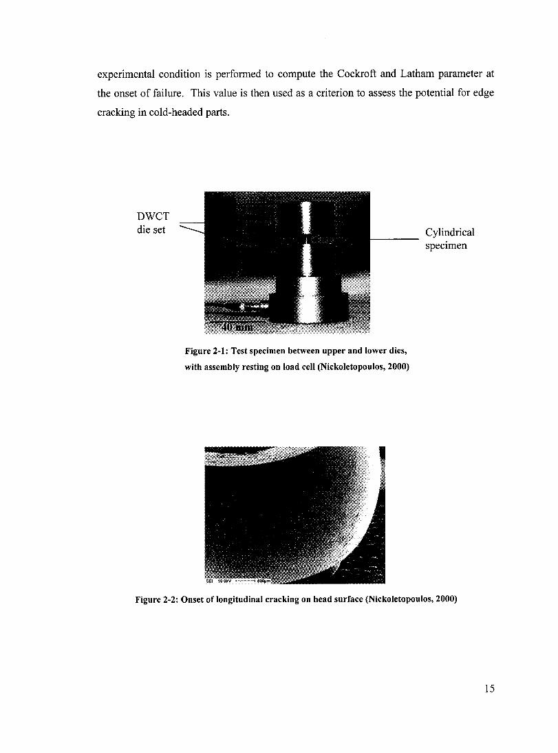
The critical Cockroft and Latham parameter C is detennined usmg a drop weight
compression test (DWCT). Typically, in such a test, cylindrical specimens are clamped at
their ends in a pocket die set, shown in Figure 2-1, and compressed. The specimens for
this particular die set have a diameter of 5.21 mm, with aspect ratios varying from 1.0 to
1.6. Experiments are usually conducted using a fixed drop height with varying dropped
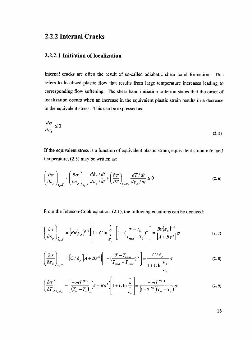
mass. The first point at which external edge cracks are visible is the one that is used to
find 'C'. The specimens are examined by a stereomicroscope with a 25x magnification.
A typical cracked specimen is shown in Figure 2-2. A finite element analysis of the
14
experimental condition is performed to compute the Cockroft and Latham parameter at
the onset of failure. This value is then used as a criterion to assess the potential for edge
cracking in cold-headed parts.
DWCT die set
Figure 2-1: Test specimen between upper and lower dies,
with assembly resting on load cell (Nickoletopoulos, 2000)
Cylindrical speCImen
Figure 2-2: Onset of longitudinal cracking on head surface (Nickoletopoulos, 2000)
15
2.2.2 InternaI Cracks
2.2.2.1 Initiation of localization
InternaI cracks are often the result of so-called adiabatic shear band formation. This
refers to localized plastic flow that results from large temperature increases leading to
corresponding flow softening. The shear band initiation criterion states that the onset of
localization occurs when an increase in the equivalent plastic strain results in a decrease
in the equivalent stress. This can be expressed as:
(2.5)
If the equivalent stress is a function of equivalent plastic strain, equivalent strain rate, and
temperature, (2.5) may be written as:
(2.6)
From the Johnson-Cook equation (2.1), the following equations can be deduced:
(2.7)
(2.8)
(2.9)
16
Using (2.7) to (2.9) in (2.6), the following is obtained:
(2.10)
This expression contains a strain hardening term, a strain rate hardening term and a
thermal softening term, sequentially. During deformation, strain and strain rate hardening
may be acted against by thermal softening. According to the aforementioned criterion,
localization will be initiated when thermal softening exceeds the strain and strain rate
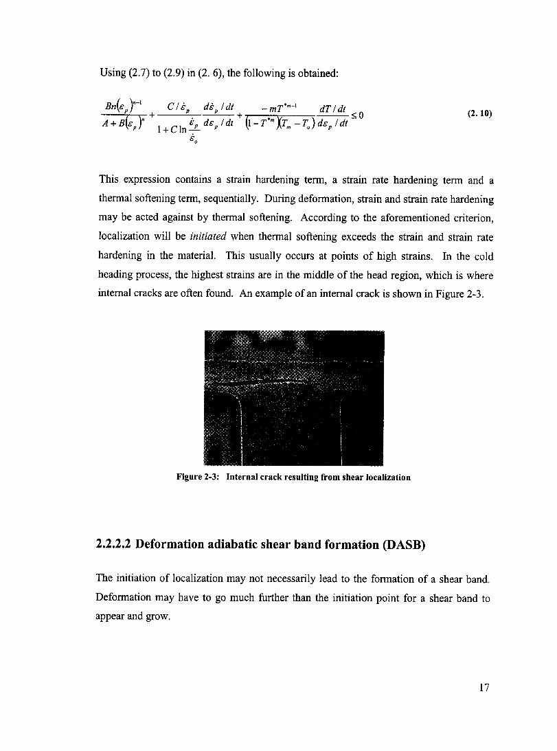
hardening in the material. This usually occurs at points of high strains. In the co Id
heading process, the highest strains are in the middle of the head region, which is where
internaI cracks are often found. An example of an internaI crack is shown in Figure 2-3.
Figure 2-3: Internai crack resulting from shear localization
2.2.2.2 Deformation adiabatic shear band formation (DASB)
The initiation of localization may not necessarily lead to the formation of a shear band.
Deformation may have to go much further than the initiation point for a shear band to
appear and grow.
17
When a shear band does form, however, it is termed a deformation adiabatic shear band
or "DASB", if the temperature rise associated with its formation remains below any
transformation temperatures. This is most likely to occur in low carbon, low alloy steels
with high ductility (Nickoletopoulos, 2000).
As mentioned in Chapter 1, there are no current fully developed criteria for shear band
formation. Different researchers, however, have suggested various possible approaches.
In the current work, the effective stress in the highest strained region is plotted and the
drop in the effective stress is used as a shear band formation criterion. As addressed in
Chapter 1, sorne authors have used 90% of peak value, others 80% (Figure 2-4). In this
work, both values are considered. Ductile damage models that are coupled with
viscoplastic models are not considered here, because they require experimental
determination of material parameters that lie beyond the sc ope of this work.
Equivalent Stress
e* p
90% or 80 % of maximum equivalent stress
Strain at which shear band is expected to form
Equivalent Plastic Strain
Figure 2-4: Deformation adiabatic shear band criterion
18
2.2.2.3 Transformation adiabatic shear band formation (TASB)
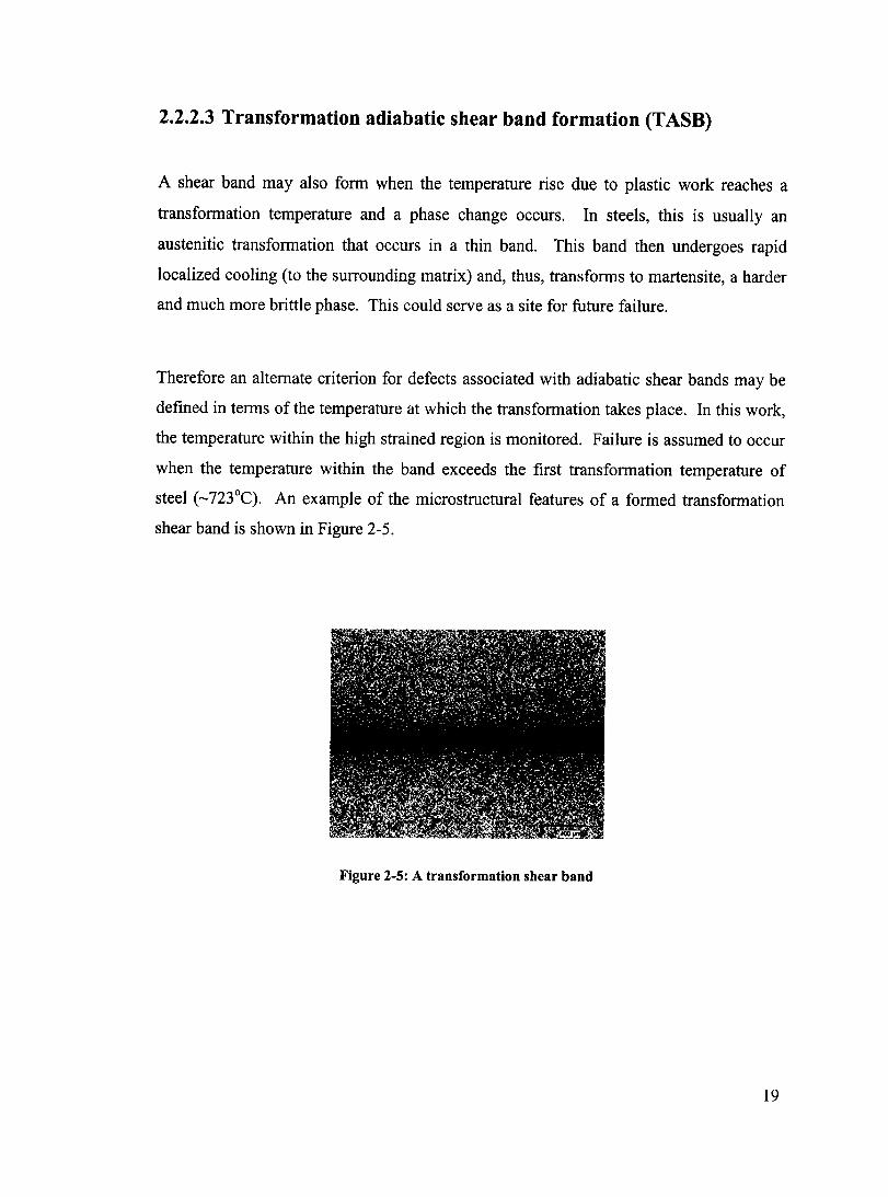
A shear band may also fonn when the temperature rise due to plastic work reaches a
transfonnation temperature and a phase change occurs. In steels, this is usually an
austenitic transfonnation that occurs in a thin band. This band then undergoes rapid
localized cooling (to the surrounding matrix) and, thus, transfonns to martensite, a harder
and much more brittle phase. This could serve as a site for future failure.
Therefore an altemate criterion for defects associated with adiabatic shear bands may be
defined in tenns of the temperature at which the transfonnation takes place. In this work,
the temperature within the high strained region is monitored. Failure is assumed to occur
when the temperature within the band exceeds the first transfonnation temperature of
steel (-723°C). An example of the microstructural features of a fonned transfonnation
shear band is shown in Figure 2-5.
Figure 2-5: A transformation shear band
19
2.3 The Taguchi Approach
2.3.1 Design of Experiments
In an optimization process, various design factors glve rise to a vast number of
experiments that have to be performed. A powerful statistical tool that allows the
designer to choose and study a set of experiments from which an optimum solution is
produced, is the design-of-experiments (DOE) method.
There are three basic approaches in the DOE. The first is the one-factor-at-a-time
approach (e.g., Fowlkes and Creveling, 1995). In this method, one factor is studied while
aU others remain fixed, and then the second factor is varied and so on. This method is
frequently used but it is time consuming and often impractical in industrial settings. The
second method is the fuU-factorial approach. Here aU possible experimental
combinations of the factor levels are performed. This may lead to an unnecessarily large
number of experiments. For instance, if four factors each with three levels are
considered, the total number of experiments will be 34 or 81. The third DOE technique
that minimizes the number of experiments needed, but aU the while providing sufficient
information for optimization, is the orthogonal array method.
Orthogonal arrays are used in the Taguchi approach. In the orthogonal array method, a
set of experiments is chosen such that the set uniformly spans the experimental space
represented by the full factorial runs. Orthogonal refers to the balance of factors so that
no factor is given more or less weight than another. It also refers to the fact that the
effects of each factor can be mathematicaUy analyzed independently of the other factors.
This is illustrated visuaUy in Table 2.1, and discussed below as an example. The
orthogonal array presented is an L-9 array, with four factors (A,B,C,D) each of which has
three-Ievel variations. There are therefore a total of 9 required experiments.
20
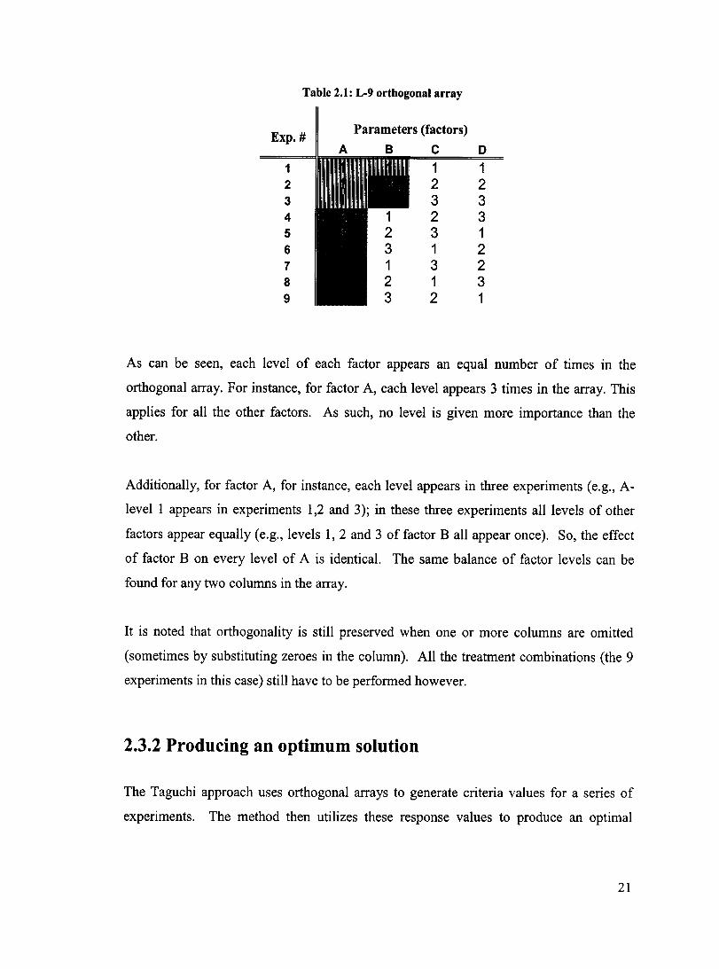
Table 2.1: L-9 orthogonal array
Exp. # Parameters (factors)
A B C 0
1 1 1 2 2 2 3 3 3 4 1 2 3 5 2 3 1 6 3 1 2 7 1 3 2 8 2 1 3 9 3 2 1
As can he seen, each level of each factor appears an equal numher of times in the
orthogonal array. For instance, for factor A, each level appears 3 times in the array. This
applies for aH the other factors. As such, no level is given more importance than the
other.
Additionally, for factor A, for instance, each level appears in three experiments (e.g., A
level 1 appears in experiments 1,2 and 3); in these three experiments aH levels of other
factors appear equaHy (e.g., levels 1,2 and 3 of factor B aH appear once). 80, the effect
of factor B on every level of A is identical. The same balance of factor levels can he
found for any two columns in the array.
It is noted that orthogonality is still preserved when one or more columns are omitted
(sometimes hy suhstituting zeroes in the column). AlI the treatment comhinations (the 9
experiments in this case) still have to he performed however.
2.3.2 Producing an optimum solution
The Taguchi approach uses orthogonal arrays to generate criteria values for a series of
experiments. The method then utilizes these response values to produce an optimal
21

combination of factor levels, usually foreign to the combinations that already exist in the
orthogonal array. This is performed by the use of so-called "factor plots".
Factor plots are essentially plots of response versus level for each factor in the
optimization search space. The underlying assumption in this approach is that no
significant interactions exist between factors. This means that the effect of an individu al
factor level on the response is assumed to be independent or minimally dependant on the
level of other factors. This could be analogous to saying that the optimum level of one
factor is not linked or conditioned to a level of another factor. This is often called a
factorial search, meaning factors can be mathematically analyzed independently of others,
which is one of the definitions of orthogonality. This then permits the averaging of
responses of one level of a factor to produce one single response for that factor level.
This averaged value is the one that is plotted for each level. If there are four factors each
with three level variations, then there are four factor plots, each having three averaged
data points. Each of these plots is then used separately to obtain the optimum level of that
factor.
Generally, one can describe three different optimization scenarios: the-smaller-the-better
type, the-greater-the-better type, or the nominal-the-best type. If a criterion requires the
maximization or minimization of a response, then in each factor plot, the level that
produces the greater or smaller mean response will be chosen. If a criterion requires a
response to approach a particular value, then the level that most closely approaches that
response is chosen.
Finally, it should be added that the same analysis can be performed by taking the non
repeatability of each response into account. This is termed 'noise' in the Taguchi
approach, and the method defines several signal (response) to noise ratios that can be
used for each of the above optimization scenarios. It is beyond the scope of this work to
describe in detail these ratios. In the upcoming chapters, the Taguchi approach is applied
on the mean responses only. Noise factors could be taken into account in future work.
N evertheless, the general framework in both cases is the same.
22
2.3.3 The predictive equation and verification of additivity
The experiments in the orthogonal array are only a fraction of the full-factorial
experiments to which the optimal solution belongs. The method allows the user to predict
the response of any combination of factors in the full space. This is done via a so-called
'predictive equation', given in (2.11). The symbol Yexp represents the total average
response of the experiments in the array; and y x , i.e. YA, YB, Ye or YD, refers to the average
response for a level of factor x.
(2.11)
This same equation can also be used to verify the additivity of the method. As can be
seen the predicted response in equation (2.11) is an additive function of the mean array
response and the average factor responses. This is true provided there are no interactions
between factors; if interactions exist, then there would be for instance multiplicative
terms in the equation. So the response of a combination is predicted via this equation,
and then the combination is performed experimentally to determine its actual value. If
the two are close, for example within 10% (Sen and Yang, 1998), then the optimization
can be considered "additive" and the assumption of insignificant interactions between
factors is valid.
If interactions between factors are significant, then the predictive equation will no longer
be additive. Significant disagreement between predicted and verified results is usually
due to this lack of additivity. The solution to interactions in the Taguchi approach is to
always minimize them by considering different approaches for arriving at the same ideal
function (Fowlkes and Creveling, 1995). Finally, it is noted that (2.11) is not only
additive but also linear with respect to the array mean and factor averages. This may not
necessarily have to be the case. The relationship could be nth order as long as there are
23
no interactive (i.e. multiplicative) terms; however, in that case, the definition of average
should probably be changed.
2.3.4 ANOV A analysis on Taguchi results
It is possible that certain factors in a design can have little or no effect on a particular
response. In that case, these factors should be excluded from the optimization process so
as not to complicate the process unnecessarily. One method of quantitatively assessing
the relative contribution of each factor to overall measured response is the analysis of
variance (ANDY A) method.
In the ANOY A method, the total sum of squares is first computed. This essentially
calculates the variance of each response in the orthogonal array around the mean of the
responses, and then sums aIl these variances. This can be represented by the formulation
below:
(2.12)
where y is the response of a row in the orthogonal array (an experiment), y is the mean
response of the array (or mean response of the experiments) and n is the number of
experiments.
Following, the individual sum of squares is ca1culated. This is the sum of the variances of
each factor level response around the mean. Therefore, for factor A for instance, the
formulation is as shown below:
(2.13)
24
where m is the number of experiments in each level of factor A and nA is the number of
levels of factor A. This procedure is repeated for aIl other factors. The percentage
contribution of each factor on the overall response, is then the ratio of the sum of squares
of each factor to the total sum of squares, multiplied by 100.
It can be said therefore that the sum of squares method attempts to numerically quantify
the variation that occurs in the overall experimental mean response due to the effects of
the factors. The greater the effect of a factor, the greater its contribution to the overall
vanance.
This is often performed within the Taguchi analysis, to determine which factors are the
'controlling' ones, and which factors contribute more to noise. Sometimes, if a factor
does not significantly affect a response, it is taken out of the array and is considered to be
a contributor of noise.
The method is very useful when multiple-criteria are considered. It is noted from the
above discussion that the conventional Taguchi approach addresses single criterion
optimization only. In multiple criteria optimization, potential conflicts between factor
levels may arise. The knowledge of the contribution of each factor to the response aids
considerably in optimizing those parameters or factors in conflict.
2.4 Multiple-Criteria Optimization
GeneraIly, it can be said that when a desirable criterion value can only be produced with
an undesirable value of another (contradiction), or when a change in a criterion value
produces a disproportional change in another (incommensurability), a decision-maker
(DM) may have to make a choice that will result in sorne positive consequences and sorne
negative ones. The aim of multiple-criteria optimization is then to maximize the positive
consequences and minimize the negative ones by arriving at a 'best compromised'
solution.
25
Multiple criteria decision-making (MCDM) methods can be divided into two broad
groups (Sen and Yang, 1998): multiple-attribute decision making (MADM) and multiple
objective decision making (MODM).
A specific approach in the multiple-criteria optimization that applies to both MADM and
MODM methods is the overall evaluation criterion (OEC) approach. The OEC is a
technique in which individual criteria are combined into an overall criterion. This is then
optimized with single objective techniques (this is sometimes called 'scalarization',
Miettinen 1999). This work utilizes OEC techniques in both MC DM groups.
The MADM methods may be described as the selection of the best alternative from
available ones. In the CUITent work, alternatives refer to factor levels. Each alternative
has different attributes. Attributes refer to average criteria values of the factor levels.
These attribut es may be weighted to ensure their comparability, and then the choice is
made amongst the alternatives. More precisely, in this work, the Taguchi approach is
first partly applied by averaging criteria values of each factor level, and then the MADM
search method is utilized. The MADM is applied to each factor, to search for that factor's
best level. In the space of one factor, the alternatives are the levels of that factor. It can
be considered that each alternative has an attribute, and the attribute is a 'vector' of
criteria values. Thus the best alternative is chosen based on the 'performance' of this
vector. Performance is defined by a TOPSIS OEC index, CL +, which will be further
detailed in section 2.4.2 and Chapter 5.
The MO DM methods are used when there is no predefined list of solutions to choose
from but rather certain requirements should be met, which are termed objectives. In this
case, a synthesis of alternatives is performed based on the prioritized objectives.
Specifically, in this work, the MO DM approach is first applied on criteria values of each
experiment, in order to tirst arrive at an OEC index, U, for each experiment. Then the
Taguchi search method is applied on each factor to choose the level of the factor that
minimizes the MODM index. This is further detailed in section 2.4.1 and in Chapter 5.
26
2.4.1 The MODM approach
The multi-objective optimization approach can be expressed ln general form as
(Chankong and Haimes, 1983):
{optimise F(X) = {j~ (X) ... J; (X) .. .fk (X)}
MODM subject to X E n (2. 14)
where X are optimization variables (factors' levels),Ji is the lh response value, Fis the set
of objective functions, n is the constrained space (e.g., design limitations). The objectives
are sometimes in conflict with one another, meaning an optimum solution of one
objective does not meet the optimum solution of another. The DM should then make a
compromise between the objectives to come up with a best solution. This gives rise to an
infinite number of compromised solutions, usually called Pareto-optimum solutions (Sen
and Yang, 1998).
2.4.1.1 The utility function method
One specifie method in the MODM approach is the utility function method, where the
multiple objectives are scalarized (cumulated) into one criterion by means of a utility
function defined as:
U(F(X)) = U(j; (X) ... J; (X} .. fk (X)) forXEn (2. 15)
where U is the utility function (i.e., an overall objective function). To arrive at a best
compromised solution then, the utility function should be optimized for ail X in n.
27
The utility function defined for a multiple-criteria problem should represent the
preferences of the decision maker among the criteria. In the simplest form, U can be
defined as a linear additive weighted function as follows:
where mi denote weighting coefficients assigned for each responsea. Weighting
coefficients may be interpreted as the relative importance of criteria for the decision
maker. However, it can be argued that this is not always the case (Roy and Mousseau,
1996). For example, dramatically different weighting vectors (lVl' lV2' ... , mk ) can result in
the same or similar Pareto optimal points, indicating that the interpretation of weights as
pure relative importance is inadequate. This implies that varying the weighting factors
linearly does not necessarily produce an equivalent linear change in the values of the
responses (Miettinen, 1999). Instead, it is suggested that lVj should be interpreted as the
rate at which the decision maker is willing to trade off values of the criteria in the space
of objectives (Hobbs, 1986).
Regardless of the difficulty addressed in predefining proper weights, the weighting
method, by means of perturbing positive weights, can be a powerful tool to generate a set
of optimum solutions. From this, as discussed previously, the decision maker can select
the final solution based on practical requirements of the problem. A systematic way of
perturbing the weights to obtain different Pareto optimal solutions is suggested in
(Chankong and Haimes, 1983).
When the decision maker is not certain about the validity of the linear form of the utility
function in a given problem, it is important to test other forms of functions for that
problem. Clearly, the performance of a utility function can change from one application
a It is sometimes preferred to normalize the original weights by dividing each weight by a constant (e.g., summation ofweights), however this has no effect on the final solution of the optimization problem.
28

to another. Two other forms of utility functions are based on the infinity norm and a
multiplicative form as follows:
U", = Max {mIC,m2F; ,aJ3F2 }
U Multiplicative = ( ml C + 1) (m2F; + 1) ( m3F2 + 1)
(2. 17)
(2.18)
In this work, the utility functions given in equations (2.16), (2.17), and (2.18) are used
and their performance with respect to the simulated cold heading process is compared.
2.4.2 The MADM approach
The MADM approach can be used in design selection problems where decisions involve
a finite number of alternatives and a set of performance attributes (Sen and Yang 1998).
The design selection can be quantitative or qualitative in nature. For instance, if the
alternatives are judgment-based (probabilistic) statements, the approach is considered to
be qualitative. If the alternatives have attributes with numerical values (deterministic),
the approach is quantitative. Thus the decision involves either choosing the most
competent alternatives or ranking them with regard to the prescribed criteria. In the
current work, the quantitative approach is used. As mentioned previously, the
alternatives are the factor levels. The attributes are the averaged criteria values that are
used to decide on the best alternative, which is the best level of each factor.
Each attribute can be given a weight (prioritized) and the alternatives may consequently
be ranked with respect to the prioritized attributes. In sorne methods, no preference
information (weights) is applicable and the decision reduces to a simple ranking of
alternatives. When weights are used in the MADM approach, sensitivity analyses may be
performed to determine an appropriate weight. In the CUITent work, the latter method is
not performed; instead, several arbitrary weights are considered in order to form different
possible solutions.
29
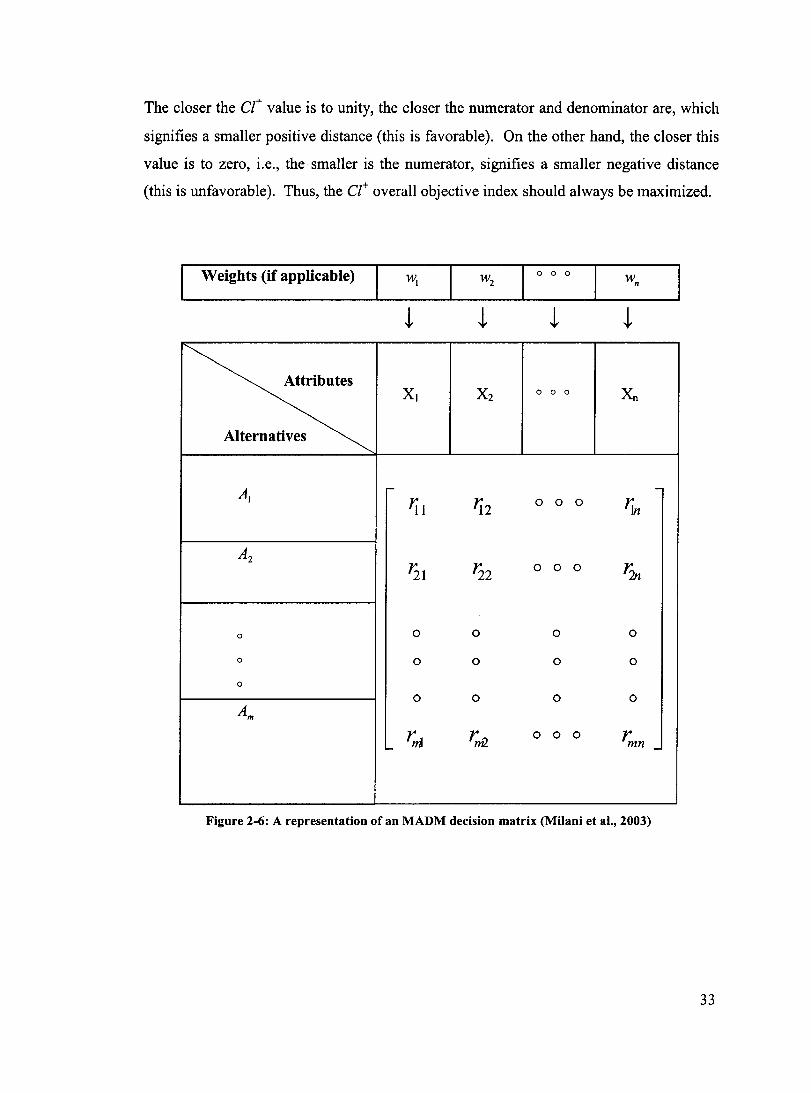
A general MADM decision matrix is shown in Figure 2-6; ri) is the value of the i th
alternative (Ai: i =:: 1, ... , m) with respect to the /h attribute (X j : j =:: l, ... , n), and wj
is
the corresponding weighting factor (Hwang 1997). Most often, in the MADM model, this
decision matrix is the only main requirement to present the input evaluation numerically.
MADM models can also be divided into two other sub-groups: compensatory and non
compensatory. Compensatory methods allow possible attribute trade-offs or interactions.
Non-compensatory methods do not. For example, if attributes are material properties,
then a certain number of these may be inversely related, e.g., the relationship between
hardness and fracture toughness (Milani et al., 2003). If the decrease in one can be
compensated for by the increase in another, then a compensatory model is appropriate.
Further complications can occur if both qualitative and quantitative attributes are
simultaneously involved in a decision. In such cases, defuzzification of the qualitative
statements (e.g.,"high", "low", etc.) is needed.
2.4.2.1 Solution method (TOPSIS)
In the current work, the TOPSIS MADM method is used. This particular method was
chosen because of its relative simplicity and speed; also, the method has been used in
many practical applications, such as selecting the optimal material for a flywheel (Dong
Hyun and Ki-Ju, 2000), analyzing a plasma-enhanced chemical vapor-deposition
(PECVD) process experiment (Tong and Su, 1997), and gear material selection (Milani et
al.,2003).
The method is based on the concept that the chosen alternative (factor level) should have
the shortest distance from an ideal point and the furthest distance from a negative ideal
point (nadir). Even though the ide al and nadir points are sometimes physically
unattainable, they can be considered as reference points, something to go to or be far
from.
30
The question though is, would it be better to choose factors that are closest to the best
solution or furthest from the worst solution? It is possible to have a point that is closest to
the best solution, and yet also close to the worst solution. Conversely, it could be furthest
from the worst solution, but not the closest to the best solution. Depending on the
application, an analyst may decide that it is better to be furthest from the worst or closest
to the best (e.g., method of weighted metrics, Miettinen 1999). Often, however, such a
decision is not straightforward. The TOPSIS method provides a third option where both
positive and negative distances are taken into account. For this purpose, a term CL+, an
overall index, is defined (see step 5).
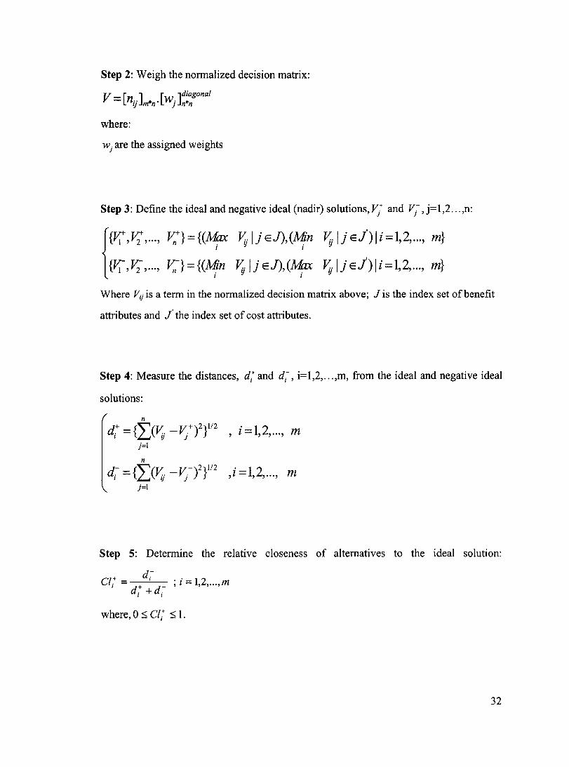
The above solution procedure can be mathematically defined in five steps as follows (Sen
and Yang, 1998).
Step 1: Transfer the decision matrix (Figure 2-6) to the normalized mode:
where:
rij is the value of the i th alternative (factor level) with respect to the /h attribute (criterion),
and nij is the corresponding normalized value. Addionally, m is the number of
alternatives and n is the number of attributes.
31
Step 2: Weigh the normalized decision matrix:
V - [ ] [ ] diagonal - nij m*n' W} n*n
where:
W j are the assigned weights
Step 3: Define the ideal and negative ideal (nadir) solutions, V/ and Vj-, j= 1,2 ... ,n:
{{~+, ~+, ... , v,;+} = {(~ Vy 1 j EJ),(Mfn Vy U EJ) 1 i = 1,2, ... , m}
1 1
{r;-,~-, ... , v,;-}={(Mfn Vy UEJ),(~ax Vy IjEJ)li=1,2, ... , m} 1 1
Where Vij is a term in the normalized decision matrix above; J is the index set of benefit
attributes and f the index set of co st attributes.
Step 4: Measure the distances, dt and di-, i=I,2, ... ,m, from the ideal and negative ideal
solutions:
n
dt = {2)Vu - ~+)2t2 , i = 1,2, ... , m j=l
n
d,:- = {"(VIj" _V;.-)2}112 . 1 2 L..J ,1 = , , ... , m j=l
Step 5: Determine the relative closeness of alternatives to the ideal solution:
Cl .+ = d j----'---- ; i = 1,2, ... , m 1 d+ d-
i + i
where,O 5 Cft 51.
32
The closer the ct value is to unit y, the closer the numerator and denominator are, which
signifies a smaller positive distance (this is favorable). On the other hand, the closer this
value is to zero, i.e., the smaller is the numerator, signifies a smaller negative distance
(this is unfavorable). Thus, the ct overall objective index should always be maximized.
Weights (if applicable) 000
Attributes Xl X2 000 Xn
Alternatives
AI r- -'il 'i2 0 0 0 rln
A2
'21 '22 0 0 0 r2n
0 0 0 0 0
0 0 0 0 0
0
0 0 0 0
Am
rnt rnû 0 o 0 rmn - -
Figure 2-6: A representation of an MADM decision matrix (Milani et al., 2003)
33
3. Numerical Analysis
This work illustrates design methodologies for the optimization of preform die geometry
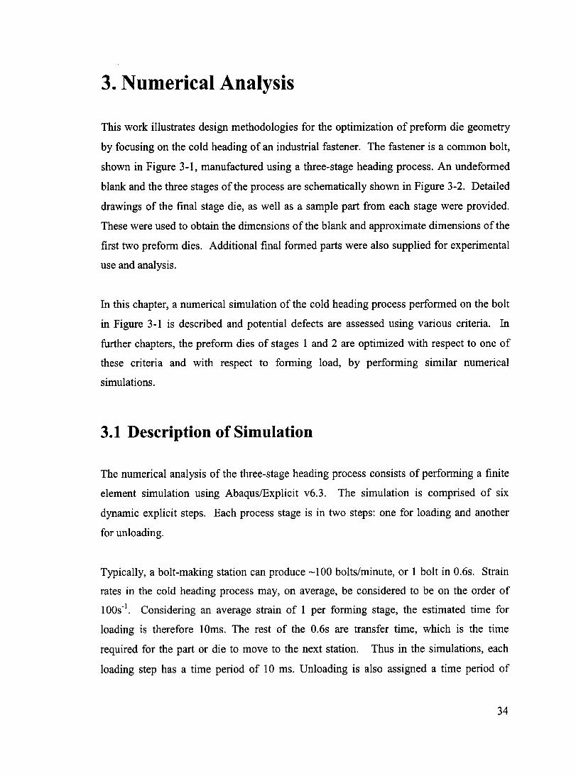
by focusing on the cold heading of an industrial fastener. The fastener is a common boit,
shown in Figure 3-1, manufactured using a three-stage heading process. An undeformed
blank and the three stages of the process are schematically shown in Figure 3-2. Detailed
drawings of the final stage die, as weIl as a sample part from each stage were provided.
These were used to obtain the dimensions of the blank and approximate dimensions of the
first two preform dies. Additional final formed parts were also supplied for experimental
use and analysis.
In this chapter, a numerical simulation of the cold heading process performed on the boIt
in Figure 3-1 is described and potential defects are assessed using various criteria. In
further chapters, the preform dies of stages 1 and 2 are optimized with respect to one of
these criteria and with respect to forming 10ad, by performing similar numerical
simulations.
3.1 Description of Simulation
The numerical analysis of the three-stage heading process consists of performing a finite
element simulation using AbaquslExplicit v6.3. The simulation is comprised of six
dynamic explicit steps. Each process stage is in two steps: one for loading and another
for unloading.
Typically, a boIt-making station can produce ~ 1 00 boIts/minute, or 1 boIt in 0.6s. Strain
rates in the cold heading process may, on average, be considered to be on the order of
100S-I. Considering an average strain of 1 per forming stage, the estimated time for
loading is therefore lOms. The rest of the 0.6s are transfer time, which is the time
required for the part or die to move to the next station. Thus in the simulations, each
loading step has a time period of 10 ms. Unloading is also assigned a time period of
34
10ms, although the blank can be considered unloaded as soon as the die loses contact with
it. The rest of the time in the unloading steps can therefore be considered as simulated
transfer time, which allows the part to relax before the next step. The full transfer time is
not included in the simulation in order to save on computational time. During the loading
stages, a constant velocity is applied. Figure 3-3 shows schematically how the steps are
employed in the simulation.
The simulation takes into account non-linear geometry and includes adiabatic heating
effects. Since the loading and unloading steps during the CHP take place on the order of
milliseconds, thermal conduction of the heat generated by plastic deformation is minimal
and it may therefore be assumed that the process is adiabatic. To verify this assumption,
the temperature drop for various steel thicknesses was calculated for a time of 10ms,
using the error function equation below (lncropera, 1996):
T b -=erf(--) To 2&
(3.1)
where T is the current temperature, Ta is the reference temperature, b is the thickness, a is
the coefficient of thermal conductivity and t is the time. The results are shown in Figure
3-4. It can be seen that in an unloading step of 10ms, temperature drop (or heat
conduction) of a localized band up to 3mm, is negligible. For a band of Imm, the
temperature drop can still be considered small (8% drop at the end of the stage). This is
especially important for the second unloading stage, just before the final deformation. In
the second stage, the localization is not expected to be below 1 mm.
Since the deformation is symmetric, an axisymmetric model is considered, the axis of
rotation passing through the center of the blank. The meshing of the blank is performed
using 4-noded continuum elements with reduced integration and hourglass control
(CAX4R). A schematic of the model assembly with the dimensions used and the meshed
blank is shown in Figure 3-5. The top half of the blank, which is the unsupported length
to be upset, is discretized into 1106 elements; the bottom half of the blank which is in
35
contact with the bottom die and does not undergo extensive deformation is discretized
into 462 elements.
The top and bottom dies are modeled as discrete rigid bodies, and the blank is defined as
a pre-drawn (16%) 1008 steel. It is taken to be an elastic-plastic material, using the
Johnson-Cook equation (given in Chapter 2) to describe the evolution of the flow stress.
Quasi-static tension tests, using a hydraulic tensile test machine, on pre-drawn specimens
were performed. The Johnson-Cook parameters A, B, and n in (2.1) were then found by
curve-fitting the stress-strain data in the plastic zone, as described in Chapter 2. This is
shown in Figure 3-6. The parameter A is the yield stress, which is found to be 490 MPa;
B and n, found from the intercept and slope of the fitted line in Figure 3-6, are 351 MPa
and 0.623, respective1y. The rate parameters C and éo are taken from (Johnson and
Cook, 1983) for a comparable steel to be 0.022 and 1, respectively, and the parameter m
is taken to be 1.00.
The bottom die is encastered as a boundary condition, and the top dies are assigned a
constant velocity such that the top and bottom dies are in complete contact at the end of a
stage. Once a stage is completed, the top die is removed and the part is allowed to relax
to establish residual stresses before the next die is brought down. Although the
deformation is predominately plastic, the use of an elastic-plastic model allows the
simulation to capture this stress state after unloading between stages as well as the final
residual stress state. As the die hits the piece, kinematic contact with fini te sliding is
established. The rigid dies are defined to be the master surfaces, and the contacting blank
edges form the slave surface. A tangential penalty friction formulation is defined with a
coefficient of friction of 0.13, obtained from the experimental work in Nickoletopoulos,
(2000). The evolution of equivalent plastic strain in the blank, obtained from the
simulation, is shown in Figure 3-7. A maximum principal stress and a temperature
contour are shown in Figure 3-8.
36
Figure 3-1: The common boit that is modeled
Figure 3-2: Schema tic of a three-stage co Id heading process
20 ,------.---------.---.-----..---------.-$tep 61
18 IJiUoad~g
Ê 16 +----t-----t----+-{S
.§. 14 +----+-----+-1: 12 +-------+---~ ~ 10 +------'-
~ 8 +---cu Q. 6 U)
Ci 4 1 2 +-~~~~~---J~-~~-~~~--~--~ 1 o -i"""'--~r__--"'"'f_----+---------'~----T-----'1
o 10 20 30
Time (ms)
40
Figure 3-3: Cold heading simulation steps
50 60
37
o ::. . .•..••. ~... 1 : -n--b-1mm 1
~ 0.5 t- 1 i~n b=3mm i 0.4 Il L_ 1
0.3 +--~~~~~~~~~
0.2 t---~~-----
1 O;~----------~ol, Time(s) ~
Figure 3-4: Temperature change for two thicknesses within the deformed blank, during unloading stages.
14.6 --:
37.9
5.5
Figure 3-5: Schema tic of the finite element model (dimensions in mm)
38

1
~-----------~---
• Experimental
-Johnson-Cook
• y = 0.623x + 5.8609
R2 = 0.9852
,-------~
-5.5 -5 -4.5 -4
In(t)
'1'11 11111
-3.5
4.5
1-' 4
3.5
3 -2.5 « 1 t)
2 -c 1.5
1
0.5 ---- 0
-3
Figure 3-6: Tensile test curve fitting for determination of Johnson Cook parameters
PEEQ
+4. 612e-01 +4.2Z8e-01 +3.644e-01 +3.'i5ge-Ol +3.075e-01 +2.69te-Ot +2.306e-Ol +1.922e-Ol +1.S37e-01 +1.153e-01 +7. 667e-02 +3.644e-02 +O.OOOe+OO
Stage 1
PEEQ
1 +t .966e+OO +1.621e+OO +1.656e+OO +1.490e+OO
, +1.325e+OO +1.15ge+OO +9.936e-Ol +6.Z63e-01 +6.629e-01 H.974e-Ol +3.320e-Ol +1.666e-01 +1.114e-03
Stage 2
PEEQ
+3.387e-+<l0 +3.1Z7e-+<l0 +2.6156e..oO +2.608e-+<l0
!1% +2.348e..oO "+2. -+<l0
+1. -+<l0 +1. ..00 +1. ..00 +1. ..00 +7. -01 +5. -01 +2. -01 +1. 02
Stage 3
Figure 3-7: Evolution of equivalent plastic strain in the blank
39
S, Xax. Principal
+5.830e-lOZ +3.35ge-t02 +8.873e-t01 -1.584e-102 -4.055e-t02 -6.527e-t02 -6.99Se-t02 -1. 147e-t03 -1.394e-103 -1. 641e-t03 -1.888e-103 -2.135e-t03 -2.383e-t03 -2.530e-t03 -2.67?e-+03 -3.1Z4e-+03
(a)
Region of highest principal
T!IIP
+6.SS0ei02 +6.11Se-+OZ +5. 67ge-+02 +S.2'14ei02 +'1 .80ge-+02 +'I.373e-+02 +3.938e-+OZ +3.S03e-+OZ +3.067e-102 +2.632ei02 +2 • 196e-+02 +1.761e-102 +1.J26eiOZ +8 .901ei01 +'I.551e-+01 +1.974eiOO
Region of highest temperature
Figure 3-8: (a) Maximum principal stress and (b) temperature contours
3.2 Assessment of Potential Defects
Bolts manufactured by this co Id heading technique are sometimes rejected because of
external (visible) defects. Parts that do pass inspections occasionally fail in service
prematurely, often because of internaI defects. It is generally understood, as discussed in
Chapter 2, that external cracks result from large tensile circumferential stresses, and
internaI cracks arise from adiabatic shear bands.
3.2.1 External Cracking
External cracking during the forming of the part can be evaluated by the Cockroft and
Latham parameter, given in (2.4). The evaluation is performed as follows. At the end of
the simulation, elements on the exterior of the head are queried for their principal stress
values. The stress-strain history of the element with the highest principal stress (indicated
in Figure 3-8a) is extracted and the evolution of the C parameter for that element is
computed from (2.4) and plotted from the point of first die contact to the final stage. The
result ofthis computation for the simulation described above is shown in Figure 3-9.
To determine whether the part would be expected to exhibit external cracks or not, a
critical value of the Cockroft and Latham parameter, C, should be used as a threshold
40
point, usually determined from experiments and simulations of a drop-weight
compression test (DWCT) as described in Chapter 2. Nickoletopoulos (2000) used this
method to obtain the parameter for a series of 1038 steels. Values of 352 MPa and 322
MPa were found for material in the as-rolled and spheroidized conditions, respectively.
Results were consistent using specimens of different aspect ratios. In the current work,
attempts were made to determine this critical value for 1008 steel, by performing a
DWCT on specimens machined from shafts of the industrial part. Even under the most
severe conditions used (28 kg mass, 2 meter drop height, 1.5 aspect ratio), no edge cracks
were observed in the laboratory specimens. Although in the DWCT experiments, a
critical value C could not be obtained, the C parameter under the most severe settings was
computed to be 620 MPa. Figure 3-9 shows that the C parameter during the heading
simulation is below this value. This is consistent with the absence of cracks in the 1008
parts examined in the laboratory.
3.2.2 InternaI Cracking
The approach to assess internaI cracks caused by adiabatic shear band formation is to first
determine the onset of localization. One way to perform this is by the use of (2.10), from
which the strain hardening term, rate hardening term, and thermal softening terms are
plotted at a location within the region of maximum strain, indicated in Figure 3-7. Figure
3-10 shows the results. It can be seen that the sum of the three terms becomes negative at
an approximate equivalent plastic strain of 2.33, which is reached relatively early in the
third stage of deformation.
Localization alone does not necessarily indicate the presence of shear bands or internaI
cracking. Strains might need to increase much further than the initiation point for shear
bands to appear. Research in this field is still ongoing, and there are currently no
universal criteria for the formation of shear bands. However, as mentioned in the
previous chapters, sorne criteria have been used based on the drop in stress in the
localized region of the shear band. Figure 3-11 is a plot of equivalent stress vs.
equivalent plastic strain for a point within the region of highest strain during the third
41
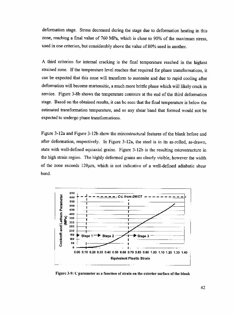
deformation stage. Stress decreased during the stage due to deformation heating in this
zone, reaching a final value of 760 MPa, which is close to 90% of the maximum stress,
used in one criterion, but considerably above the value of 80% used in another.
A third criterion for internaI cracking is the final temperature reached in the highest
strained zone. If the temperature level reaches that required for phase transformations, it
can be expected that this zone will transform to austenite and due to rapid cooling after
deformation will become martensitic, a much more brittle phase which willlikely crack in
service. Figure 3-8b shows the temperature contours at the end of the third deformation
stage. Based on the obtained results, it can be seen that the final temperature is below the
estimated transformation temperature, and so any shear band that formed would not be
expected to undergo phase transformations.
Figure 3-12a and Figure 3-12b show the mircostructural features of the blank before and
after deformation, respectively. In Figure 3-12a, the steel is in its as-rolled, as-drawn,
state with well-defined equiaxial grains. Figure 3-12b is the resulting microstructure in
the high strain region. The highly deformed grains are clearly visible, however the width
of the zone exceeds 120/-lm, which is not indicative of a well-defined adiabatic shear
band.
650 ... ~ 600 E 550 l! 500
~ 450
E 400 cv -. .c cv 350 .... Q. j :::E 300 'C -- 250 1: cv 200
~ 150 ~ 100 (,) o ()
50
o
~ - .J - - - - - - - . CoL from DWCT - - - - - - - - - -1 • 1 1 /' 1 1 /' 1 1 ,/ 1 1 ./ 1 1 L , ,
~ , '/ , ./ .. ~ Stage 1 --. Stage 2 /' : ... Stage 3
r-./ .
• ...-- : 0.00 0.10 0.20 0.30 0.40 0.50 0.60 0.70 0.80 0.90 1.00 1.10 1.20 1.30 1.40
Equivalent Plastic Strain
Figure 3-9: C parameter as a function of strain on the exterior surface of the blank
42
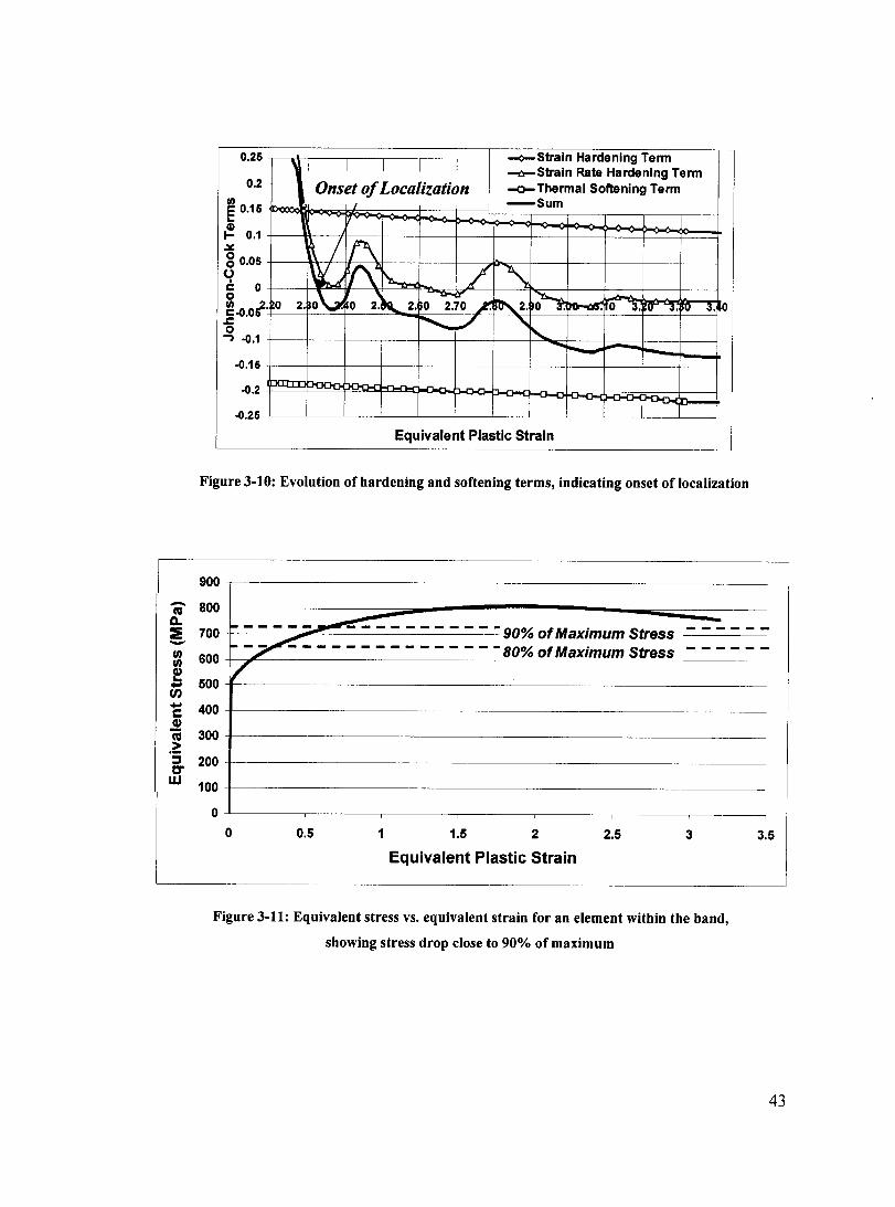
-ca CL :e -II) II)
! ... en ... c Q)
Cii .~ ~ 0" W
0.25 ~Strain Hardening Terrn , 1 1 1 1 1 ___ Strain Rate Hardening Term
0.2 - Onset of Localization ~ Thermal Softening Terrn
ê 0.15 1 -Sum
~ 0.1
/ ~ ~
80.05 () L f\ ~ / ~ 1
0 C 0
2. ov. 0 2.~ 2. ~ If'
~2. .~ J>.
~-o.O~' 0 o 2. 0;- o ~. 1'-=' 0 3.~1T -;i; ~ 3.1J0 .c ""-./ " 0 "-.., -0.1 -- --0.15
-0.2
-0.25
Equivalent Plastic Strain
Figure 3-10: Evolution of hardening and softening terms, indicating onset of localization
900
800
700
600
500
1- - - - --~ - - - - - - - - 90% of Maximum Stress -------1--~- - - - - - - - - - - - - -80% of Maximum Stress ------
r 400
300
200
100
0 o 0.5 1 1.5 2 2.5 3 3.5
Equivalent Plastic Strain
Figure 3-11: Equivalent stress vs. equivalent strain for an element within the band,
showing stress drop close to 90% of maximum
43
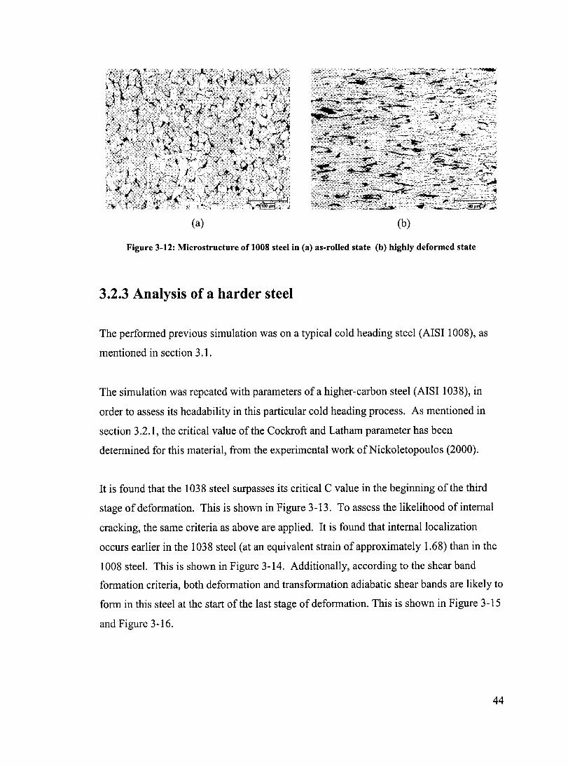
(a) (b)
Figure 3-12: Microstructure of 1008 steel in (a) as-rolled state (b) highly deformed state
3.2.3 Analysis of a harder steel
The perfonned previous simulation was on a typical cold heading steel (AISI 1008), as
mentioned in section 3.1.
The simulation was repeated with parameters of a higher-carbon steel (AISI 1038), in
order to assess its headability in this particular cold heading process. As mentioned in
section 3.2.1, the critical value of the Cockroft and Latham parameter has been
detennined for this material, from the experimental work of Nickoletopoulos (2000).
It is found that the 1038 steel surpasses its critical C value in the beginning of the third
stage of defonnation. This is shown in Figure 3-13. To assess the likelihood of internaI
cracking, the same criteria as above are applied. It is found that internallocalization
occurs earlier in the 1038 steel (at an equivalent strain of approximately 1.68) than in the
1008 steel. This is shown in Figure 3-14. Additionally, according to the shear band
fonnation criteria, both defonnation and transfonnation adiabatic shear bands are likely to
fonn in this steel at the start of the last stage of defonnation. This is shown in Figure 3-15
and Figure 3-16.
44
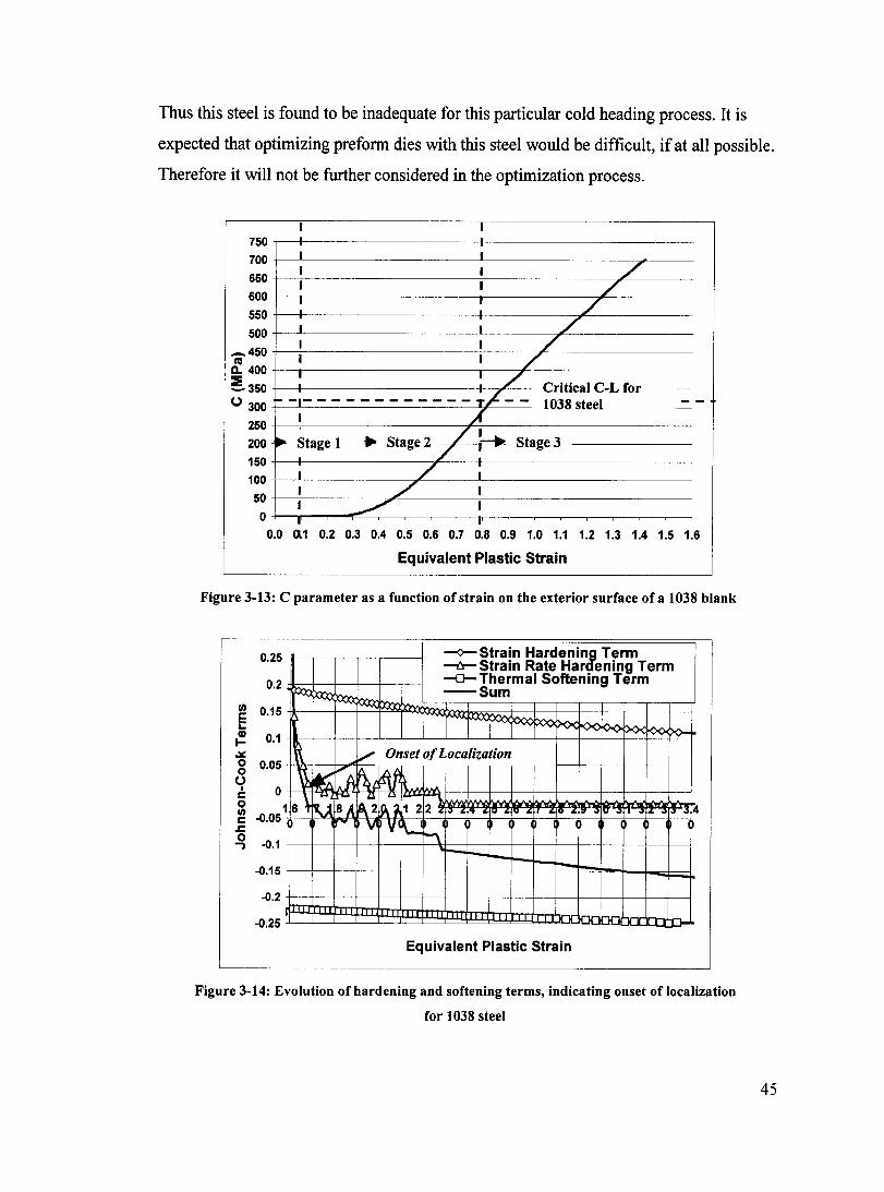
Thus this steel is found to be inadequate for this particular cold heading process. It is
expected that optimizing preform dies with this steel would be difficult, if at aU possible.
Therefore it will not be further considered in the optimization process .
750
700
650
600
550
500 _450 cv
Q. 400
~350 0 300
250
200
150 100
50
o
. . ; .
1
1 1 ./ 1 1 / 1 1 / 1 1 ./ 1 1 / 1 1 / 1 1 /' Critical C-L for -
~-I------------T~-- 1038 steel -.,.(
-
1
~ Stage 1 .. Stage 2 / 1 • / ~
Stage 3
; / ; 1 ./' 1 1 .-/ 1 l' l'
0.0 0.1 0.2 0.3 0.4 0.5 0.6 0.7 0.8 0.9 1.0 1.1 .1.2 1.3 1.4 1.5 1.6
Equivalent Plastic Strain
Figure 3-13: C parameter as a function of strain on the exterior surface of a 1038 blank
0.25 -<>-Strain Hardenin~ Term --tr- Strain Rate Har ening Term
0.2 -0-Thermal Softening Term too --Sum ~ )(ny
III 0.15 E J'>. LA CI) 0.1 .... ~ V Onset of Localization 0 0.05
~ 0
~ 1-'.11 r\t W. 0 ,., ~ 1 0 1-C ;-u
~~ 1.> , ........ '""""'\
0 16 ~ ~ BA ~~ 1 2 2 ... 1" "Il 1/) ." ... ..... ... 1" ... "'1" ... .. "1"" " C -0.05 "V \Il V' \..: ~ 0 ~ ..., -0.1 -
-0.15
-0.2
-0.25 J-
Equivalent Plastic Strain
Figure 3-14: Evolution of hardening and softening terms, indicating onset of localization
for 1038 steel
45
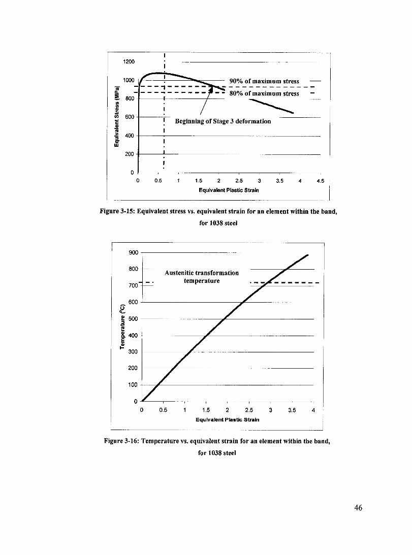
1200,-----~---------------------------------------
1000 L ~ ............... ~ 90% of maximum stress ---
'l : : : : ::! : : : : : : l' - ;- 80%-or m~xim-u; ;;r~s; - :
i soo : / ~---
e 1 ~ û) 600 . B .. fS 3 d ç • ë egmnmg 0 tage e.ormatlon oS!
.~ 400 +-----~--------------------------------------:::J
lE' 1
200+-----~1-------------------------------------
o 0.5 1.5 2 2.5 3 3.5 4 4.5
Equivalent Plastic Strain
Figure 3-15: Equivalent stress vs. equivalent strain for an element within the band,
for 1038 steel
900
SOO
700
600 6' ~
f 500 :::J ... I! 8. 400 E {!
300
200
100
0 0
Austenitic transformation temperature
0.5 1.5 2 2.5
Equivalent Plastic Strain
3 3.5 4
Figure 3-16: Temperature vs. equivalent strain for an element within the band,
for 1038 steel
46
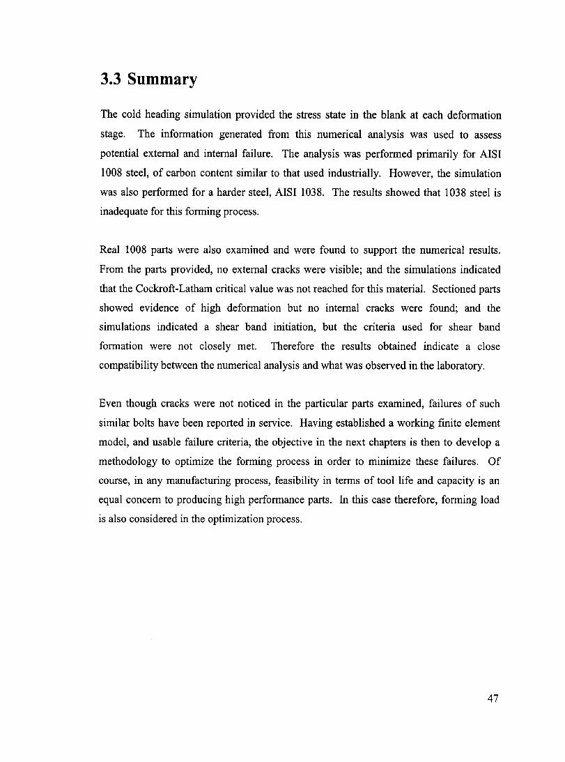
3.3 Summary
The cold heading simulation provided the stress state in the blank at each deformation
stage. The information generated from this numerical analysis was used to assess
potential external and internaI failure. The analysis was performed primarily for AISI
1008 steel, of carbon content similar to that used industrially. However, the simulation
was also performed for a harder steel, AISI 1038. The results showed that 1038 steel is
inadequate for this forming process.
Real 1008 parts were also examined and were found to support the numerical results.
From the parts provided, no external cracks were visible; and the simulations indicated
that the Cockroft-Latham critical value was not reached for this material. Sectioned parts
showed evidence of high deformation but no internaI cracks were found; and the
simulations indicated a shear band initiation, but the criteria used for shear band
formation were not closely met. Therefore the results obtained indicate a close
compatibility between the numerical analysis and what was observed in the laboratory.
Even though cracks were not noticed in the particular parts examined, failures of such
similar bolts have been reported in service. Having established a working finite element
model, and usable failure criteria, the objective in the next chapters is then to develop a
methodology to optimize the forming process in order to minimize these failures. Of
course, in any manufacturing process, feasibility in terms of tool life and capacity is an
equal concern to producing high performance parts. In this case therefore, forming load
is also considered in the optimization process.
47

4. Single Criteria Optimization
In this chapter, the forming process described in Chapter 3 is optimized with respect to
two separate criteria: part failure and forming load. The objective here is to find
independent solutions for the criteria and then to compare their results.
Referring to the design parameters of Bakhshi-Jooybari et al. (1996) addressed in Chapter
1, the corner radius of the deformed blank and the final ratio in the current work are fixed,
since the optimization is for one particular boit shape. Therefore, since the third stage
corresponds to the final shape of the product, it do es not involve design variations. The
only design parameter that is to be optimized is then the upset ratio (ratio of unsupported
length to diameter of the blank) in the first and second stages. Two geometrical
dimensions are therefore varied, independently, on each preform die, and a third
dimension is changed to keep the total volume conserved. Processing parameters are kept
constant and similar to the actual manufacturing process. The coefficient of friction is set
to a value of 0.13 (Nickoletopoulos, 2000). No pre-heat temperature is considered, and
since the material is not significantly dependant on strain-rate, the type of machine as
described by Bakhshi-Jooybari et al. (1996) is not particularly important for this
optimization. Additionally, the material is fixed to a 1008 steel. Therefore, the design
parameters are reduced to four geometrical dimensions on the preform dies, shown in
Figure 4-1.
The number of stages in the current work is kept at three throughout the optimization
process. This is primarily because the actual manufacturing process, as discussed in
Chapter 3, uses three stages to form the boIt. In general, there are many reasons why
several stages are performed in the heading process, versus just one. One reason is to
avoid buckling and flash (the formation of unwanted materiaI). The rules given by
Naujoks and FabeI, described in Chapter 1, are for that purpose, for example. In the
current work, Rule 1 can be applied, since the upset length is less than three times the
blank diameter. In addition, the upset ratio (ratio of the unsupported length - length to be
48
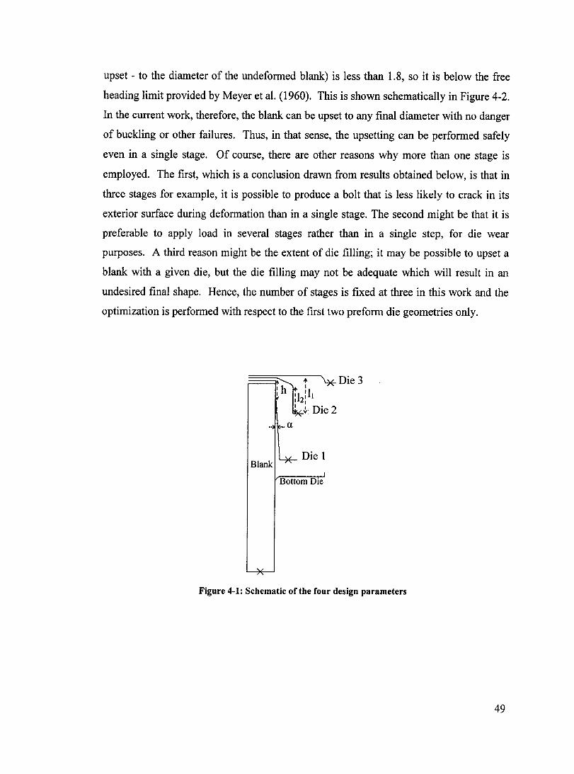
upset - to the diameter of the undefonned blank) is less than 1.8, so it is below the free
heading limit provided by Meyer et al. (1960). This is shown schematically in Figure 4-2.
In the current work, therefore, the blank can be upset to any final diameter with no danger
of buckling or other failures. Thus, in that sense, the upsetting can be perfonned safely
even in a single stage. Of course, there are other reasons why more than one stage is
employed. The first, which is a conclusion drawn from results obtained below, is that in
three stages for example, it is possible to produce a bolt that is less likely to crack in its
exterior surface during defonnation than in a single stage. The second might be that it is
preferable to apply load in several stages rather than in a single step, for die wear
purposes. A third reason might be the extent of die filling; it may be possible to upset a
blank with a given die, but the die filling may not be adequate which will result in an
undesired final shape. Hence, the number of stages is fixed at three in this work and the
optimization is perfonned with respect to the first two prefonn die geometries only.
l1t+ ,*Die3
: h Il :11 1 2: 1 -!t. Die 2
.. ... a
Die 1 Blank
Bottom Die
Figure 4-1: Schematic of the four design parameters
49
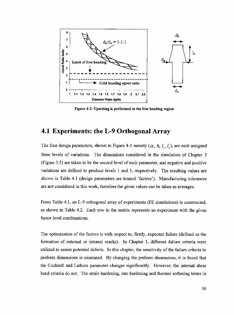
8
7
6 o l! .2 5 o ~ 4 Limit of free heading ~:::-J\i~ __ 13 + ~~~-
2
·····r······································ 1 ~ Cold heading upset ratio
o+-~~~--~~~~--~~~~~
1 1.1 1.2 1.3 1.4 1.5 1.6 1.7 1.8 1.9 2 2.1 2.2
Dlameter Ratio dg/do
Figure 4-2: Upsetting is performed in the free heading region
4.1 Experiments: the L-9 Orthogonal Array
The four design parameters, shown in Figure 4-1 namely (a, h, Il' 1), are each assigned
three levels of variations. The dimensions considered in the simulation of Chapter 3
(Figure 3.5) are taken to be the second level of each parameter, and negative and positive
variations are defined to produce levels 1 and 3, respectively. The resulting values are
shown in Table 4.1 (design parameters are termed 'factors'). Manufacturing tolerances
are not considered in this work, therefore the given values can be taken as averages.
From Table 4.1, an L-9 orthogonal array of experiments (FE simulations) is constructed,
as shown in Table 4.2. Each row in the matrix represents an experiment with the given
factor level combinations.
The optimization of the factors is with respect to, firstly, expected failure (defined as the
formation of external or internaI cracks). In Chapter 3, different failure criteria were
utilized to assess potential defects. In this chapter, the sensitivity of the failure criteria to
preform dimensions is examined. By changing the preform dimensions, it is found that
the Cockroft and Latham parameter changes significantly. However, the internaI shear
band criteria do not. The strain hardening, rate hardening and thermal softening terms in
50
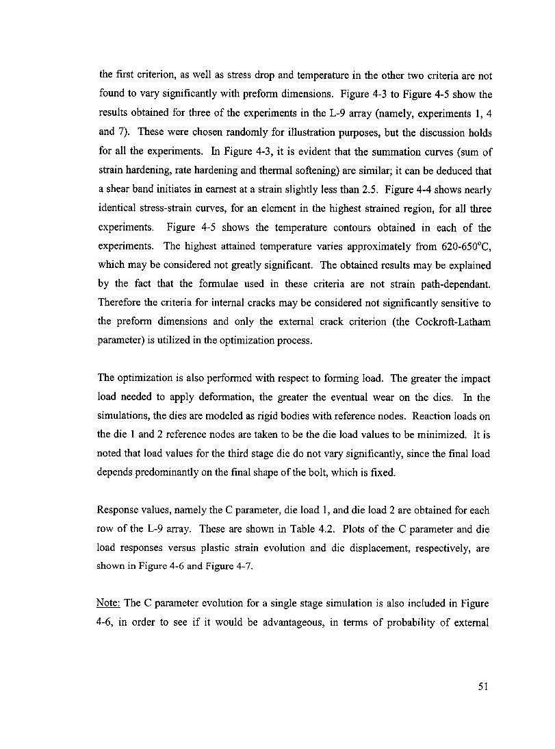
the first criterion, as weIl as stress drop and temperature in the other two criteria are not
found to vary significantly with preform dimensions. Figure 4-3 to Figure 4-5 show the
results obtained for three of the experiments in the L-9 array (namely, experiments 1, 4
and 7). These were chosen randomly for illustration purposes, but the discussion holds
for aIl the experiments. In Figure 4-3, it is evident that the summation curves (sum of
strain hardening, rate hardening and thermal softening) are similar; it can be deduced that
a shear band initiates in earnest at a strain slightly less than 2.5. Figure 4-4 shows nearly
identical stress-strain curves, for an element in the highest strained region, for aIl three
experiments. Figure 4-5 shows the temperature contours obtained in each of the
experiments. The highest attained temperature varies approximately from 620-650°C,
which may be considered not greatly significant. The obtained resuIts may be explained
by the fact that the formulae used in these criteria are not strain path-dependant.
Therefore the criteria for internaI cracks may be considered not significantly sensitive to
the preform dimensions and only the external crack criterion (the Cockroft-Latham
parameter) is utilized in the optimization process.
The optimization is also performed with respect to forming load. The greater the impact
load needed to apply deformation, the greater the eventual wear on the dies. In the
simulations, the dies are modeled as rigid bodies with reference nodes. Reaction loads on
the die 1 and 2 reference nodes are taken to be the die load values to be minimized. It is
noted that load values for the third stage die do not vary significantly, since the final load
depends predominantly on the final shape of the boIt, which is fixed.
Response values, namely the C parameter, die load 1, and die load 2 are obtained for each
row of the L-9 array. These are shown in Table 4.2. Plots of the C parameter and die
load responses versus plastic strain evolution and die displacement, respectively, are
shawn in Figure 4-6 and Figure 4-7.
Note: The C parameter evolution for a single stage simulation is also included in Figure
4-6, in order to see if it would be advantageous, in terms of probability of external
51

cracking, to use three stages instead of one. It is clear that an improvement to the single
stage C value can be made using three stages.
Levels
1 2 3
Table 4.1: Factors and their level variations. Factors
a (degrees) h (mm) 11 (mm) h (mm)
0.8 4.0 7.2
2.5 5.0 7.5
5.5 7.2 9.0
3 4 5
Table 4.2:The L-9 orthogonal arral: and numerical res~onse of ex~eriments.
Exp. # Factors Numerical RespoDse
a h lt h C ~MPa} FI ~kN} Fz ~kN} 1 1 1 1 1 633.47 137.07 413.60 2 1 2 2 2 596.54 157.35 323.69 3 1 3 3 3 555.45 131.38 243.69 4 2 1 2 3 527.22 352.44 252.69 5 2 2 3 1 583.64 293.64 263.38 6 2 3 1 2 528.08 287.30 306.07 7 3 1 3 2 558.45 417.68 306.57 8 3 2 1 3 458.20 404.90 302.87 9 3 3 2 1 534.10 373.36 418.20
0.2
0.15 1/)
E .. 0.1 CI) 1-~
0.05 0 0 0
1 0 C
0 1/) 2 c -0.05 ~ 0 ..,
-0.1
-0.15
\ ~ .1 .L: ~~ M. 2. SO 2. 70~ ~ 90 3. GO 3. 10 3. 20 3. ~O 3.~1 'r-r~ ~~2.
-..J lFj ~ ~ ~ ~ ~
"IJ"'" "" ~ ~ ~.
" ~ o
-0.2 Equivalent Plastic Strain
Figure 4-3: Shear band initiation criterion for experiments 1,4 and 7
52
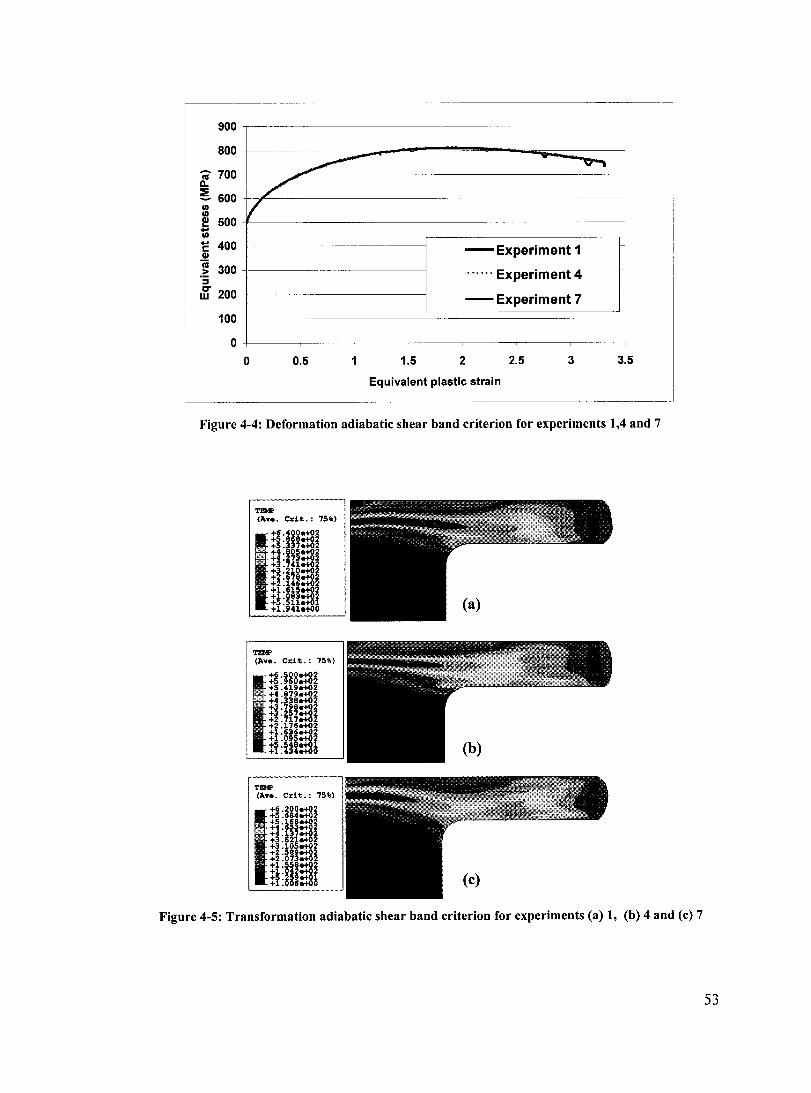
1:0 ,..-------------------------------------
1 800 ~----.~~~~~~~--~~ ca 700 +-----~~---------------------------------
~ 600 +-~~~--------------------------------------------~ 500 ~~----------------------------.. CIl
-Experiment1] ........... Experiment 4
--Experiment 7
--,
2 2.5 3 3.5
Equivalent plastic strain
Figure 4-4: Deformation adiabatic shear band criterion for experiments 1,4 and 7
Tl!H' (Ave. Crit.: 75"',
+5.868e+02 ". +5.337e+02
1 +6.400.+02
,.:: !P~~~~ +3.'be+02 +3.210e+02
- +2. 678e+02 +2.146e+02 +1.615e+02 +l.083e+02 +5.511e+Ol +l.941e+OO
Tl!H' (Av •• Crit.: 15%)
1·· +6 .500e+02 !~:Ug::g~ +4.879e+02 +4.338e+02
-- +3. 798e+02 +3.257e+02 +2.717e+02 +2.176e+02 +1.636e+02 +1.09~::gi !Î:~he+Oà
Tl!H' (Ave. Crit.: 75~)
i-- +6 .200e+02
+5.684e+02
--. :::tnE8î !~:m::g~ !~:m::g~ +1.SS8e+02 +1.042.+02
!tm~~
l
1
Figure 4-5: Transformation adiabatic shear band criterion for experiments (a) 1, (b) 4 and (c) 7
53
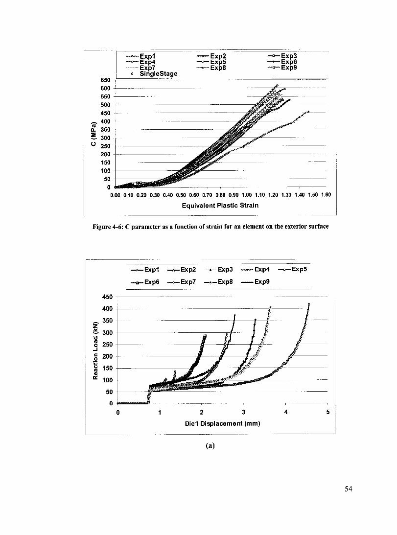
,------r==~===E=X=P=1=========-+-====EX=P=2==========-O-=,==--EE=XX=-Pp==36--==------l---0- Exp4 -~ Exp5
'Exp7 -Exp8 --Exp9 o SingleStage
650~============================================
600 550t---~~------------------------~-~~~
500 ~~~----------
450 +------------------------------~~~ _ 400 +-----------
~ 350 +--------
~ 300 (.) 250 +~----------__:
200 ~-----------150 ~----------100 +--------------:
5~~~lijiil~--~--~~--~~--~~--~~--~--~-0.00 0.10 0.20 0.30 0.40 0.50 0.60 0.70 0.80 0.90 1.00 1.10 1.20 1.30 1.40 1.50 1.60
Equivalent Plastic Strain
Figure 4-6: C parameter as a function of strain for an element on the exterior surface
-o-Exp1 _+_Exp2 _Exp3 _Exp4 -o-Exp5[
-ç,-Exp6 -o-Exp7 -.-Exp8 -Exp9 1
J
450
400
_ 350 z e. 300 "C ni 250 0
..J c 200 0
; u 150 ni CIl
0::: 100
50
0
0 1 2 3 4 5
Die1 Displacement (mm)
(a)
54

------
--Exp1 -)K-Exp2 -.t-Exp3 -o-Exp4 -Exp5
_Exp6 .......ç....-Exp7 -:c-Exp8 -+-Exp9
450
400
Z 350 ~
- 300 "C cu
250 0 ...1 c: 200 0 ..
150 CJ cu 11)
0:: 100
50
0 , 0 2 4 6 8 10 12 14 16
Die2 Displacement (mm)
(b)
Figure 4-7: (a) Dielload 1 response (b) Die load 2 response
4.2 Conventional Taguchi Optimization
4.2.1 Factor Plots
Having obtained three response values for each row of the L-9 matrix, the aim at this
point is to use this data to search through the entire 81-experiment space for the best
combination of factor levels. Using the conventional Taguchi optimization, this can be
performed for each response separately, to obtain three optimal combinations. This is
achieved by the use of the so-called "factor plots".
As discussed in Chapter 2, a single response can be obtained for each level of each factor
by averaging its three responses (each factor level appears three times in the matrix). For
instance, C values of the three experiments that inc1ude a-Ievel 1 are averaged to produce
one value for the response of this level of a. This is repeated for each level and factor,
for C and force responses. The results are shown in Table 4.3. These are then plotted to
55
produce three factor-plots, as shown in Figure 4-8 and Figure 4-9. It is noted that l, and
h are not included in the analysis for die load 1 because these parameters (belonging to
stage 2 of deformation) have no physical influence on die load 1.
The factor levels that minimize the response values are subsequently chosen to produce
three optimal combinations, one with respect to C, the other two with respect to die loads.
The independent optimums and their simulation (actual) results are shown in Table 4.4.
4.2.2 Additivity of the method
The above method for choosing an optimum solution relies on the assumption that no
interactions exist between factors. Therefore, as discussed in Chapter 2, an additive
equation can be constructed to predict results of any combination, or any of the 81
experiments. The general equation (2.11) can be rewritten as (4.1), for this optimization.
It is used to verify the additivity of the experiments with respect to each criterion (i.e., the
C parameter and preform die loads), or, in other words, the validity of the aforementioned
assumption. A simulation is performed using each of the suggested optimum
combinations in Table 4.4 and this is compared to the results obtained using the
predictive equation. Table 4.5 shows the results.
(4.1)
It is seen that the maximum differences between the actual and predicted values are less
than 8%. Discrepancies can be possibly due to slight interactions between the factors.
They could also be due to a deviation from linearity of the actual predictive model. It
should be noted that although the predictive equation used here is linear, it could in fact
be non-linear but still remain additive with respect to each factor. As mentioned in
Chapter 2, this would not contradict the Taguchi assumption of minimal interactions, as
long as there are no multiplicative terms in the equation. In this case, it can be said that a
relatively reasonable approximation can be made with this linear equation because the
discrepancies are relatively small, i.e. <10%.
56
4.2.3 ANOV A Analysis
An analysis of variance is perfonned on the average responses of the factor levels, to
detennine the percent contribution of each factor on the criteria. The response values of
each criterion are first averaged for the nine experiments. The total sum of squares, using
(2.12), is then calculated for each criterion. Following, the sum of squares of each factor
is calculated using (2.13). The ratio of the two sum of squares denotes the contribution of
each factor on the value of the criteria. The results of the ANOVA analysis are shown in
Table 4.6 to Table 4.8. It is noted that because II and h are not inc1uded in the ANOV A
analysis of die 1, the array is not saturated. This leaves four degrees of freedom for
experimental error, interactions and other factors. This is denoted as "error" in Table 4.7.
4.3 Discussion
As can be seen in Table 4.6, the factors that contribute the most to the C parameter are a
and h. The prefonn cone angle, a, has the highest contribution. From Figure 4-8, the
larger the cone angle, the smaller the C value, or the less likelihood for edge cracking.
The larger the value of h, the smaller the C value. The parameter h is related to the cut
off angle of die 2; it indicates that a square-like geometry is more favorable than a
tetrahedral-like geometry with respect to the value of C.
The ANOVA analysis in Table 4.7 shows that the most significant contributor for die
load 1 is also a. From Figure 4-9(a), it is noted that, in contrast to the C parameter,
minimizing the die load requires minimizing a. This is an apparent conflict in the choice
of parameter levels.
Table 4.8 shows that the detennining parameters for die load 2 are h and h. the latter
being the greatest contributor to the load value. Parameter a also seems to significantly
affect die load 2. From Figure 4-9(b), minimizing die load 2 requires maximizing both l,
and h, and maintaining an average value of a.
57
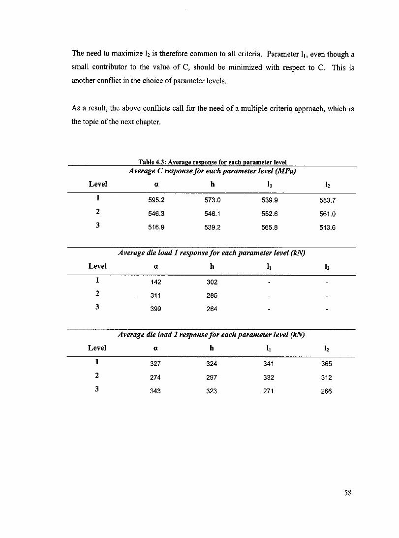
The need to maximize lz is therefore common to aIl criteria. Parameter Il, even though a
small contributor to the value of C, should be minimized with respect to C. This is
another conflict in the choice of parameter levels.
As a result, the above conflicts caU for the need of a multiple-criteria approach, which is
the topic of the next chapter.
Table 4.3: Average response for each parameter level Average C response for each parameter level (MPaj
Level a h 1. lz
1 595.2 573.0 539.9 583.7
2 546.3 546.1 552.6 561.0
3 516.9 539.2 565.8 513.6
Average die load 1 response for each parameter level (kN)
Level a h h lz
1 142 302
2 311 285
3 399 264
Average die load 2 responsefor each parameter level (kN)
Level a h 1. lz
1 327 324 341 365
2 274 297 332 312
3 343 323 271 266
58
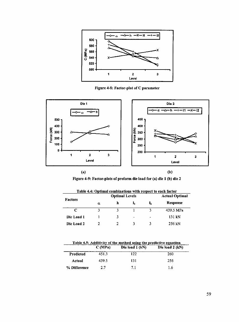
500
400 Z ~ 300 CI)
~ 200 ~
100
600
580
~ 560 ::E 0' 540
520
500
Ole 1
I~a ---b- h -~-I1 -+- 121
1 2 3 level
Figure 4-8: Factor-plot of C parameter
450
400 z ~ 350 CI)
~ 300 o u.. 250
0le2
I~a -ô-h -+-11 -~-12
o+-------~------~----~. 200+--------r------~------__, 1 2
level
(a)
3 2
level
(b)
Figure 4-9: Factor-plots ofpreform die load for (a) die 1 (b) die 2
Table 4.4: O~timal combinations with res~ect to each factor
Factors Optimal Levels Actual Optimal
a h Il h Response
C 3 3 3 439.5 MPa
Die Load 1 3 131 kN
Die Load 2 2 2 3 3 256kN
Table 4.5: Additivity of the method using the predictive equation C (MPa) Die load 1 (kN) Die load 2 (kN)
Predicted 451.3 122 260
Actual 439.5 131 256
% Difference 2.7 7.1 1.6
3
59
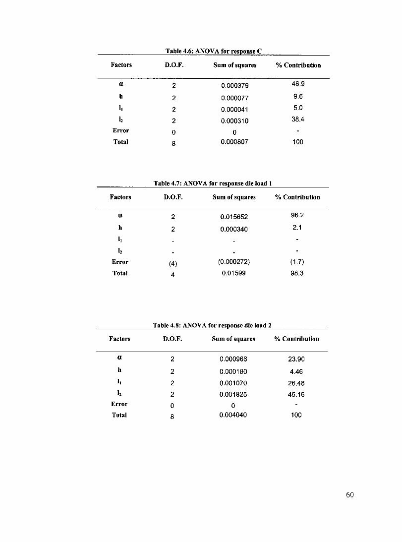
Table 4.6: ANOV A for response C
Factors D.O.F. Sum of squares % Contribution
a 2 0.000379 46.9
h 2 0.000077 9.6
1) 2 0.000041 5.0
h 2 0.000310 38.4
Error 0 0 Total 8 0.000807 100
Table 4.7: ANOVA for response die load 1
Factors D.O.F. Sum of squares % Contribution
a 2 0.015652 96.2
h 2 0.000340 2.1
1)
12
Error (4 ) (0.000272) (1.7)
Total 4 0.01599 98.3
Table 4.8: ANOV A for response die load 2
Factors D.O.F. Sum of squares % Contribution
a 2 0.000966 23.90
h 2 0.000180 4.46 1) 2 0.001070 26.48
h 2 0.001825 45.16 Error 0 0 Total 8 0.004040 100
60
5. Multiple Criteria Optimization
As illustrated in the previous chapter, the conventional Taguchi method can be used to
optimize preform die geometries with respect to one eriterion. When combinations
optimized for different criteria are contradictory, a multiple criteria approach becomes
necessary. As discussed in Chapter 1, there exists in the literature a range of different
approaches. In this chapter, the multiple-criteria techniques described in Chapter 2 are
applied within the conventional Taguchi method and their performance with respect to
preform die geometry optimization is analyzed.
As mentioned in Chapter 2, the OEC approach is applied in this work, in which individual
criteria are eombined into an overall criterion. This is then optimized with single
objective techniques. The steps to follow when using an OEC in the common Taguchi
method can be described as follows:
(a) Find the best combination oflevels for each criterion separately.
(b) Compare the optimal solutions and verify which factors produce the same optimal
levels for aIl criteria.
(c) If there are contradictions, combine the criteria into one overall index and then
analyze this index (Roy, 2001).
In the CUITent work, aIl approaches to simultaneously minimize the C parameter and the
preform die loads generally follow these three steps. Step (a) was performed in Chapter
4, with the results displayed in Table 4.4. The following verification holds for step (b).
It can be seen from the optimal solutions in Table 4.4 that parameter h shows no conflict
with any of the criteria. Factor h shows slight conflict with respect to the criterion F2.
From the ANOVA analysis in Table 4.8, however, the effect ofthis parameter on die load
2 is not significant «5%). Thus, level 3 for factor h may also be considered optimal for
aIl criteria. The other two factors (a and Il) are in an apparent conflict and the multiple-
61
criteria solution should arrive at a compromise between them. Thus step (c) becomes
necessary.
5.1 Selected Methods
The approach for multiple-criteria decision making (MCDM), is divided into two groups,
as discussed in Chapter 2: multiple-objective decision-making (MODM) and multiple
attribute decision-making (MADM) methods. In the current work, both categories will be
examined. Within the former category, the utility function method is mostly used as an
OEC tool for the Taguchi technique, and it is also employed here. Within the latter
category, the use of the TOPSIS method as another OEC tool is introduced in this work.
Finally, a comparative analysis of the two methods is performed.
Remark: the Taguchi approach in multiple response problems can be understood in both
subgroups. It can be categorized in the MODM or multiple objective optimization
analysis since the final solution (combination of factor levels) is normally none of the
alternatives initially prescribed by orthogonal arrays. On the other hand, it can be
categorized in the MADM analysis since the set of feasible factor levels is discrete,
predetermined and finite. Clearly, ifa full-factorial approach (i.e. the full 81 experiments)
is applied, then the optimization reduces to a pure MADM approach, as the best solution
will be among the generated alternatives.
5.2 Utility Function Methods
In this method, multiple criteria are converted into an overall index by means of a
predefined utility function. This function utilizes weighting coefficients that represent the
decision maker's preferences among the criteria.
62
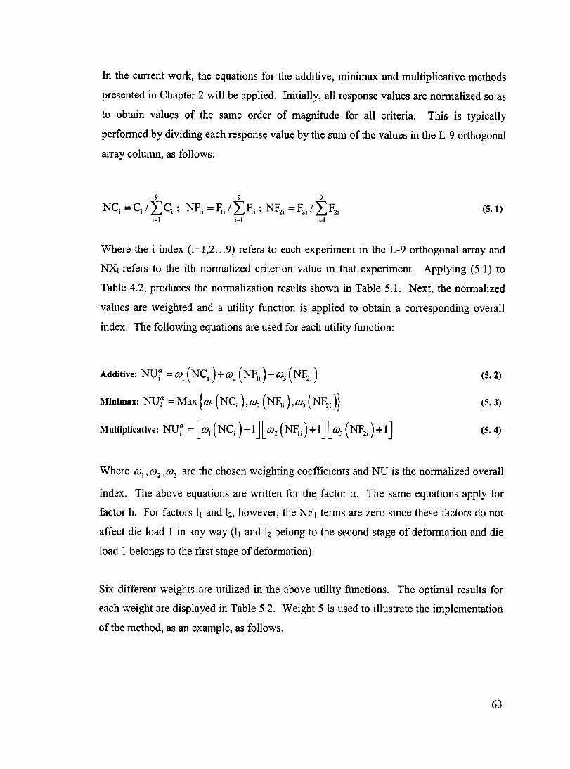
In the current work, the equations for the additive, minimax and multiplicative methods
presented in Chapter 2 will be applied. Initially, all response values are norrnalized so as
to obtain values of the same order of magnitude for all criteria. This is typically
perforrned by dividing each response value by the sum of the values in the L-9 orthogonal
array column, as follows:
9 9 9
NCi =CJICi ; N~i =~JI~i; NF2i =F2i /IF2i (5.1) i=1 i=1 i=1
Where the i index (i=1,2 ... 9) refers to each experiment in the L-9 orthogonal arrayand
NXj refers to the ith norrnalized criterion value in that experiment. Applying (5.1) to
Table 4.2, produces the normalization results shown in Table 5.1. Next, the normalized
values are weighted and a utility function is applied to obtain a corresponding overall
index. The following equations are used for each utility function:
Minimax: NUf = Max{CüI (NCi ),Cü2 (NF;i),Cü3 (NF2i )}
Multiplicative: NUf = [ Cül (NCi ) + 1] [ Cü2 (NF;i ) + 1] [ Cü3 (NF2i ) + 1 ]
(5.2)
(5.3)
(5.4)
Where Cü l , Cü2 , Cü3 are the chosen weighting coefficients and NU is the normalized overall
index. The above equations are written for the factor a. The same equations apply for
factor h. For factors Il and h, however, the NF 1 terrns are zero since these factors do not
affect die load 1 in any way (11 and h belong to the second stage of deforrnation and die
load 1 belongs to the first stage of deformation).
Six different weights are utilized in the above utility functions. The optimal results for
each weight are displayed in Table 5.2. Weight 5 is used to illustrate the implementation
of the method, as an example, as follows.
63
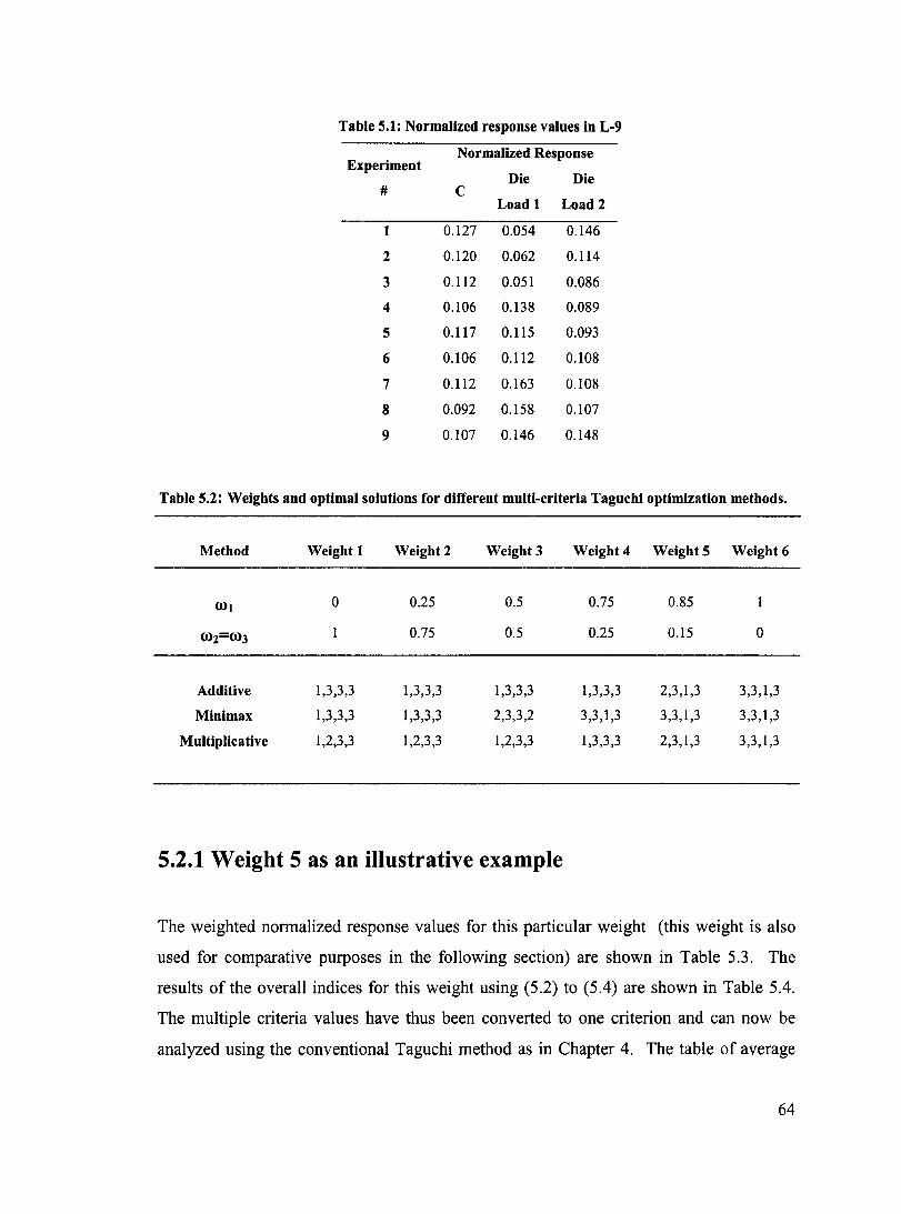
Table 5.1: Normalized response values in L-9
Experiment Normalized Response
Die Die # C
Load 1 Load2
1 0.127 0.054 0.146
2 0.120 0.062 0.114
3 0.112 0.051 0.086
4 0.106 0.138 0.089
5 0.117 0.115 0.093
6 0.106 0.112 0.108
7 0.112 0.163 0.108
8 0.092 0.158 0.107
9 0.107 0.146 0.148
Table 5.2: Weights and optimal solutions for different multi-criteria Taguchi optimization methods.
Method Weight 1 Weight 2 Weight3 Weight 4 Weight 5 Weight 6
(01 0 0.25 0.5 0.75 0.85
O>Z=0>3 0.75 0.5 0.25 0.15 0
Additive 1,3,3,3 1,3,3,3 1,3,3,3 1,3,3,3 2,3,1,3 3,3,1,3
Minimax 1,3,3,3 1,3,3,3 2,3,3,2 3,3,1,3 3,3,1,3 3,3,1,3
Multiplicative 1,2,3,3 1,2,3,3 1,2,3,3 1,3,3,3 2,3,1,3 3,3,1,3
5.2.1 Weight 5 as an illustrative example
The weighted normalized response values for this particular weight (this weight is also
used for comparative purposes in the following section) are shown in Table 5.3. The
results of the overall indices for this weight using (5.2) to (5.4) are shown in Table 5.4.
The multiple criteria values have thus been converted to one criterion and can now be
analyzed using the convention al Taguchi method as in Chapter 4. The table of average
64
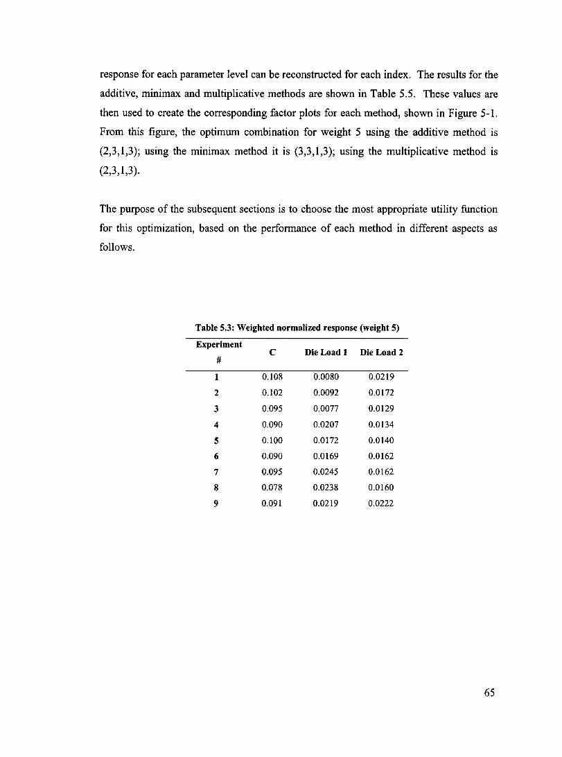
response for each parameter level can be reconstructed for each index. The results for the
additive, minimax and multiplicative methods are shown in Table 5.5. These values are
then used to create the corresponding factor plots for each method, shown in Figure 5-1.
From this figure, the optimum combination for weight 5 using the additive method is
(2,3,1,3); using the minimax method it is (3,3,1,3); using the multiplicative method is
(2,3,1,3).
The purpose of the subsequent sections is to choose the most appropriate utility function
for this optimization, based on the performance of each method in different aspects as
follows.
Table 5.3: Weighted normalized response (weight 5)
Experiment C Die Load 1 Die Load 2
#
1 0.108 0.0080 0.0219
2 0.102 0.0092 0.0172
3 0.095 0.0077 0.0129
4 0.090 0.0207 0.0134
5 0.100 0.0172 0.0140
6 0.090 0.0169 0.0162
7 0.095 0.0245 0.0162
8 0.078 0.0238 0.0160
9 0.091 0.0219 0.0222
65
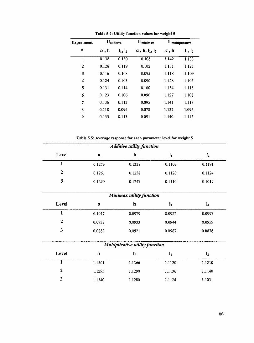
Table 5.4: Utility function values for weight 5
Experiment Uadditlve Uminimax U multiplicative
# a,h 1., h a, h, 1., h a,h 1., 12
1 0.138 0.130 0.l08 1.142 1.133
2 0.l28 0.119 0.102 1.131 1.121
3 0.116 0.108 0.095 1.118 1.109
4 0.124 0.l03 0.090 1.128 1.105
5 0.131 0.114 0.100 1.134 1.115
6 0.123 0.106 0.090 1.127 1.108
7 0.136 0.112 0.095 1.141 1.113
8 0.118 0.094 0.078 1.122 1.096
9 0.135 0.113 0.091 1.140 1.115
Table 5.5: Average response for each parameter level for weight 5
Additive utility function
Level a h Il h
1 0.1273 0.1328 0.1103 0.1191
2 0.1261 0.l258 0.1120 0.l124
3 0.l299 0.1247 0.1110 0.1019
Minimax utility function
Level a h Il h
1 0.1017 0.0979 0.0922 0.0997
2 0.0933 0.0933 0.0944 0.0959
3 0.0883 0.0921 0.0967 0.0878
Multiplicative utility function
Level a h Il 12
1 1.1301 1.1366 1.1120 1.1210
2 1.1295 1.1290 1.1136 1.1140
3 1.1340 1.1280 1.1124 1.1031
66

0.140 I-o-a -tr-h -:(-11 -+- 12 1 >< 0.135 CI)
~~ " 0.130 -::: .5 CI) 0.125 ,:: 0.120 .
~~~ :: " 0.115
" C'\I 0.110 ~
0.105 + 0.100
2 3
level
(a)
0.110 ' I-o-a -tr-h -)1(-11 -+- 12 1 >< 0.105 ' CI)
"
~~ ,5 0.100 >< C'\I 0.095 E '2 0.090 'Ë ~
0.085
0.080 1 2 3
level
(b)
I~a -tr-h -)1(-11 -+- 12 1 1.140
~ 1.135 ~ ~1.130 ~tF ~ ~ 1.125 ~ 1.120 + _______ :a 1.115 ~ ~ 1.110)1( ~-)I( E 1.105 ~ ::l 1.100 ~ ___________ --. _____ ---,
(c)
2
level 3
Figure 5-1: Factor plots for weight 5 (a) Uaddltlve, (b) Umlnlmm (c) Umultlpllcatlve
67
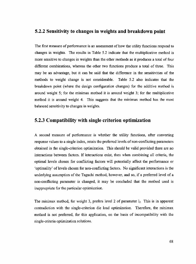
5.2.2 Sensitivity to changes in weights and breakdown point
The first measure of performance is an assessment of how the utility functions respond to
changes in weights. The results in Table 5.2 indicate that the multiplicative method is
more sensitive to changes in weights than the other methods as it produces a total of four
different combinations, whereas the other two functions pro duce a total of three. This
may be an advantage, but it can be said that the difference in the sensitivities of the
methods to weight change is not considerable. Table 5.2 also indicates that the
breakdown point (where the design configuration changes) for the additive method is
around weight 5; for the minimax method it is around weight 3; for the multiplicative
method it is around weight 4. This suggests that the minimax method has the most
balanced sensitivity to changes in weights.
5.2.3 Compatibility with single criterion optimization
A second measure of performance is whether the utility functions, after converting
response values to a single index, retain the preferred levels of non-conflicting parameters
obtained in the single-criterion optimization. This should be valid provided there are no
interactions between factors. If interactions exist, then when combining aIl criteria, the
optimal levels chosen for conflicting factors will potentially affect the performance or
'optimality' of levels chosen for non-conflicting factors. No significant interactions is the
underlying assumption of the Taguchi method, however, and so, if a preferred level of a
non-conflicting parameter is changed, it may be concluded that the method used IS
inappropriate for the particular optimization.
The minimax method, for weight 3, prefers level 2 of parameter h. This is in apparent
contradiction with the single-criterion die load optimization. Therefore, the minimax
method is not preferred, for this application, on the basis of incompatibility with the
single-criteria optimization solutions.
68
In order to compare the other two methods, weights 1 and 6 are then examined. Surely
the weight 1 combinations should be compatible with the single die load optimizations;
and similarly weight 6 should be compatible with the single C optimization. It is seen
that the additive method produces compatible results. The multiplicative method chooses
level 2 of h for weight 1. This is still compatible (it corresponds to the preferred choice
when optimizing die load 2 alone). However, as discussed before, since h has little effect
on die load 2, the chosen combination can be considered comparable to the (1,3,3,3)
combination preferred by the additive method for weight 1. For weights 2 and 3, the
multiplicative method still prefers level 2 of factor h. On the other hand, the additive
method prefers level 3 for factor h. Since this level improves two out of the total three
criteria (see also Table 4.4), this choice may be more rational.
The additive method is therefore preferred over the multiplicative method from the above
reasoning, and it is also chosen because of its simplicity. AdditionaIly, the additive utility
function decouples the criteria such that they can be evaluated independently (there are no
interaction terms between criteria).
5.2.4 Extent of parameter lev el differentiation
In aIl three utility function forms, often the difference between performances of parameter
levels is very small. For instance, the multiplicative method chooses a (2,3,1,3)
combination for weight 5, i.e. level 2 for parameter 0,. However, level 2 could easily be
replaced by level 1 for 0" as their normalized utility values are within a fraction of a
percent (1.129 versus 1.130, see Table 5.5). This would produce a seemingly equivalent
combination (1,3,1,3). The C and force values for these two combinations are, however,
significantly different (more than 20%). Parameter a has a strong effect on the individual
criteria. It can be said, therefore, that a possible drawback of these utility functions is that
sometimes their differentiation between factor levels is not prominent; whereas based on
the actual response values, the difference between the levels is significant.
69
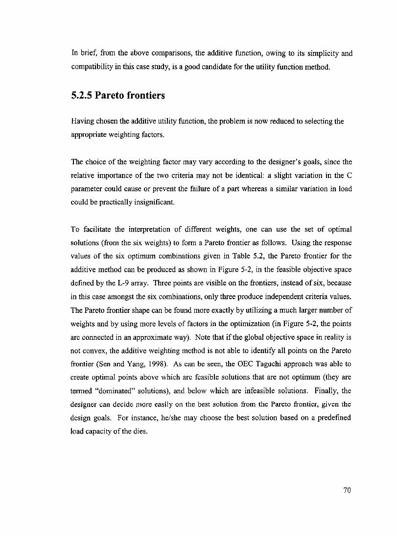
In brief, from the above comparisons, the additive function, owing to its simplicity and
compatibility in this case study, is a good candidate for the utility function method.
5.2.5 Pareto frontiers
Having chosen the additive utility function, the problem is now reduced to selecting the
appropriate weighting factors.
The choice of the weighting factor may vary according to the designer's goals, since the
relative importance of the two criteria may not be identical: a slight variation in the C
parameter could cause or prevent the failure of a part whereas a similar variation in load
could be practically insignificant.
To facilitate the interpretation of different weights, one can use the set of optimal
solutions (from the six weights) to form a Pareto frontier as follows. Using the response
values of the six optimum combinations given in Table 5.2, the Pareto frontier for the
additive method can be produced as shown in Figure 5-2, in the feasible objective space
defined by the L-9 array. Three points are visible on the frontiers, instead of six, because
in this case amongst the six combinations, only three produce independent criteria values.
The Pareto frontier shape can be found more exactly by utilizing a much larger number of
weights and by using more levels of factors in the optimization (in Figure 5-2, the points
are connected in an approximate way). Note that if the global objective space in reality is
not convex, the additive weighting method is not able to identify aIl points on the Pareto
frontier (Sen and Yang, 1998). As can be seen, the OEC Taguchi approach was able to
create optimal points above which are feasible solutions that are not optimum (they are
termed "dominated" solutions), and below which are infeasible solutions. Finally, the
designer can decide more easily on the best solution from the Pareto frontier, given the
design goals. For instance, he/she may choose the best solution based on a predefined
load capacity of the dies.
70
650
600
lsso :::Il! 0' SOO
1 1 1. 1 : .
Die1
Local Feasible Objective Space
,;
• __ 11 ______ _
450
400+---r-~~~--~---r--~--T---'
6S0
600
l550 :::Il! 0' SOO
100 150 200 250 300 350 400 450 500
Force (kN)
(a)
Die 2
Local Feasible Objective Space
1 1 1 :. 1 • •
450
400+---r-~~~--~--~---r---r--~
100 150 200 250 300 350 400 450 500
Force (kN)
(h)
Figure 5-2: Pareto frontier between (a) C and F for Die 1, (b) C and F for Die 2
5.3 A new OEC approach within the Taguchi method:
TOPSIS
The TOPSIS method is in the class of multiple-attribute decision-making models. It is
based on the concept that the chosen alternative (factor level) should have the shortest
distance from an ide al point and the furthest distance from a negative ideal (nadir) point.
As discussed in Chapter 2, these models are applied to discrete optimization spaces from
which optimum levels of factors are selected with respect to given criteria. They are
therefore applicable within the Taguchi method, considering that the optimization space is
the full-factorial space (81 experiments in the L-9 case). It is noted that the TOPSIS
method assumes that attributes (criteria) take either monotonically increasing or
71
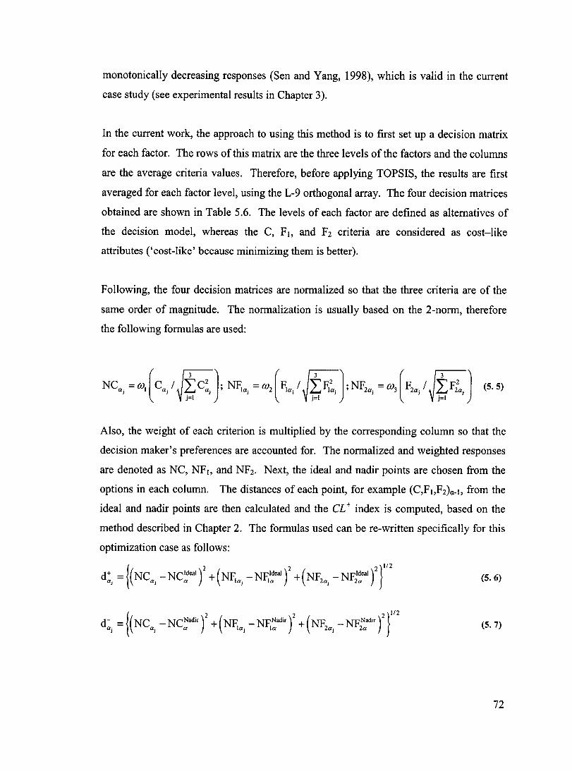
monotonically decreasing responses (Sen and Yang, 1998), which is valid in the current
case study (see experimental results in Chapter 3).
In the current work, the approach to using this method is to first set up a decision matrix
for each factor. The rows of this matrix are the three levels of the factors and the columns
are the average criteria values. Therefore, before applying TOPSIS, the results are first
averaged for each factor level, using the L-9 orthogonal array. The four decision matrices
obtained are shown in Table 5.6. The levels of each factor are defined as alternatives of
the decision model, whereas the C, FI, and Fz criteria are considered as cost-like
attributes ('cost-like' because minimizing them is better).
Following, the four decision matrices are normalized so that the three criteria are of the
same order of magnitude. The normalization is usually based on the 2-norm, therefore
the following formulas are used:
AIso, the weight of each criterion is multiplied by the corresponding column so that the
decision maker's preferences are accounted for. The normalized and weighted responses
are denoted as Ne, NF 1, and NFz. Next, the ideal and nadir points are chosen from the
options in each column. The distances of each point, for example (C,Fl,Fz)a-l, from the
ideal and nadir points are then ca1culated and the CL + index is computed, based on the
method described in Chapter 2. The formulas used can be re-written specifically for this
optimization case as follows:
{
2 2 2 }112 d+ = (NC _NCldeal) +(NR _NRldeal) +(NF _NFldeal)
a j a J a laj la 2aJ 2a (5.6)
{
2 2 2 }112 d- = (NC _NCNadir) +(NR _NRNadir) +(NF _NFNadir) ai ai a lai la 2aj 2a (5.7)
72
(5.8)
Similarly to section 5.2, the method is re-iterated for each weight with the final optimal
solutions shown in Table 5.7. The results for weight 5 are used as an illustrative example.
Using (5.5), and the decision matrices in Table 5.6, the normalized responses for weight 5
are shown in Table 5.8. The solution mechanism using (5.6) to (5.8), for weight 5 is
illustrated graphically in Figure 5-3 to Figure 5-6. Figure 5-3a shows the normalized
decision matrix points along with the ideal and nadir points, and the distances between
them, for factor a. Figure 5-3b shows the value of the CL + index for each level
(alternative) of factor a. For comparison, the results ofthe additive model are also shown
in the same graph. Similarly, Figure 5-4 to Figure 5-6 illustrate the results for the other
three factors.
As a larger CL + value is preferred, the optimum combination for weight 5 based on the
TOPSIS method is (1,3,1,3). The following is a comparison with the additive method for
this weight.
5.3.1 The TOPSIS method compared to the additive utility
function method
Figure 5-4 to Figure 5-6 show no contradiction for parameters h, II and h, between the
additive and TOPSIS methods. The lowest NU value corresponds to the highest CL +
value. However, for parameter a (Figure 5-3) this is not the case. The TOPSIS method
chooses level 1 for a, the additive method chooses level 2. In examining Figure 5-4
again, it is noticed that leve12 of a is in fact the closest to the ideal point (d+ = 0.055). On
the other hand, it is also the closest to the nadir point (d- = 0.053). TOPSIS then
disregards this level, and chooses the next best one, which is levell ofa (d+ = 0.071, d- =
73
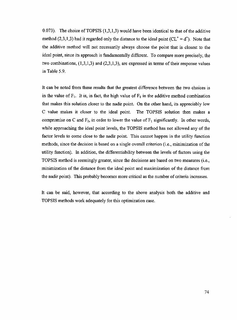
0.073). The choice of TOPSIS (1,3,1,3) would have been identical to that of the additive
method (2,3,1,3) had it regarded only the distance to the ideal point (CL+ = d+). Note that
the additive method will not necessarily always choose the point that is closest to the
ideal point, since its approach is fundamentally different. To compare more precisely, the
two combinations, (1,3,1,3) and (2,3,1,3), are expressed in terms of their response values
in Table 5.9.
It can be noted from these results that the greatest difference between the two choices is
in the value of FI. It is, in fact, the high value of Flin the additive method combination
that makes this solution closer to the nadir point. On the other hand, its appreciably low
C value makes it closer to the ideal point. The TOPSIS solution then makes a
compromise on C and F2, in order to lower the value of FI significantly. In other words,
while approaching the ideal point levels, the TOPSIS method has not allowed any of the
factor levels to come close to the nadir point. This cannot happen in the utility function
methods, since the decision is based on a single overall criterion (i.e., minimization of the
utility function). In addition, the differentiability between the levels of factors using the
TOPSIS method is seemingly greater, since the decisions are based on two measures (i.e.,
minimization of the distance from the ideal point and maximization of the distance from
the nadir point). This probably becomes more critical as the number of criteria increases.
It can be said, however, that according to the above analysis both the additive and
TOPSIS methods work adequately for this optimization case.
74
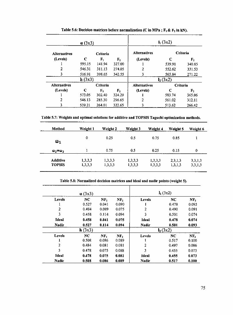
Table 5.6: Decision matrices before normalization (C in MPa ; FI & Flin kN).
a (3x3) II (3x2)
Alternatives Criteria Alternatives Criteria
(Levels) C FI Fl (Levels) C F2
1 595.15 141.94 327.00 1 539.91 340.85 2 546.31 311.13 274.05 2 552.62 331.53
3 516.91 398.65 342.55 3 565.84 271.22
h (3x3) h (3x2) Alternatives Criteria Alternatives Criteria
(Levels) C FI F2 (Levels) C F2
1 573.05 302.40 324.29 1 583.74 365.06 2 546.13 285.30 296.65 2 561.02 312.11
3 539.21 264.01 322.65 3 513.62 266.42
Table 5.7: Weights and optimal solutions for additive and TOPSIS Taguchi optimization methods.
Method Weight 1 Weight 2 Weight3 Weight4 Weight 5 Weight 6
0 0.25 0.5 0.75 0.85 6)1
c.l2=c.l3 0.75 0.5 0.25 0.15 0
Additive 1,3,3,3 1,3,3,3 1,3,3,3 1,3,3,3 2,3,1,3 3,3,1,3 TOPSIS 1,3,3,3 1,3,3,3 1,3,3,3 1,3,3,3 1,3,1,3 3,3,1,3
Table 5.8: Normalized decision matrices and ideal and nadir points (weight 5).
a (3x3) Il (3x2)
Levels NC NFI NF2 Levels NC NF2
1 0.527 0.041 0.090 1 0.478 0.093 2 0.484 0.089 0.075 2 0.490 0.091
3 0.458 0.114 0.094 3 0.501 0.074
Ideal 0.458 0.041 0.075 Ideal 0.478 0.074 Nadir 0.527 0.114 0.094 Nadir 0.501 0.093
h (3x3) l:z (3x2) Levels NC NFI NF2 Levels NC NF2
1 0.508 0.086 0.089 1 0.517 0.100 2 0.484 0.081 0.081 2 0.497 0.086
3 0.478 0.075 0.088 3 0.455 0.073
Ideal 0.478 0.075 0.081 Ideal 0.455 0.073 Nadir 0.508 0.086 0.089 Nadir 0.517 0.100
75
Ut r\'·~:::::-~ ....... ~..__--_t-----l 0.62
0.47
(a)
TOPSIS - -11- -Additive 1
0.52.,..-------------,. 0.131
0.51
0.5
CL+ 0.49
0.48
0.47
0.46 -
• 0.130
0.129
0.128 NU
0.127
0.126
0.125
-----40.124
2
a-Ievel
(b) Figure 5-3: (a) Graphical representation of TOPSIS solution and (b) comparison with the additive
method, for design factor a using weight 5.
U1O---~------I"'" TOPSIS· ... Additive 1
0..101 0.010 r----------~ 0.135
U01 0.8 • '\, o ... ~ 0.6
CL+ o .... 0.130
NU OAM 0.4
OA7G 0.2
0
OA111-------~-t------------O-~----7--~~ 0.013 ""'1 0.079
0.014
0.125 .. .. +-__ ....,.. ___ .,..-_L_-+ 0.120
2 3
h-Ievel
(a) (b) Figure 5-4: (a) Graphical representation of TOPSIS solution and (b) comparison with the
additive method, for design factor h using weight 5.
76

(J Z
U z
0.51 11_3
TCfSIS - •• • Additivel 0.019 Nadir
0.6 0.113 0.50 0.5
0.112 0.4 ... 0.49 0.023 . .. .. • CL+0.3 • 0.111 NJ
11_1 0.2
, OAB
Ideal 0.019 0.1 0.110
0.47 0 0.109 0.07 D.OB 0.09 0.10 2 3
NF2 11-level
(a) (b)
Figure 5-5: (a) Graphical representation of TOPSIS solution and (b) comparison with the additive method, for design factor Il using weight 5.
0.54 12
_1
TOPSIS • -•• Additiive 1 0.52 0.13 0.50
0.8 0.12 0.4B . -0.46
0.6 .. CL+ • 0.11 NU Ideal 0.4 • 0.44 , ..
0.42 0.2 0.10
0.06 0.07 D.OB 0.09 0.10 0.11 0 0.09
NFz 2 3
(a) 12-level
(b) Figure 5-6: (a) Graphical representation of TOPSIS solution and (b) comparison with the
additive method, for design factor 12 using weight 5.
Table 5.9: Response values of additive and TOPSIS methods for weight 5.
METHOD C (MPa)
Additive 470 Weighted relative distance Jrom 3.5%
single criteria solutions
TOPSIS 530 Weighted relative distance Jrom 14.9%
single criteria solutions
Response
FI (kN)
291 20.7%
122 0%
F2 (kN)
260 0%
313 3.1%
77
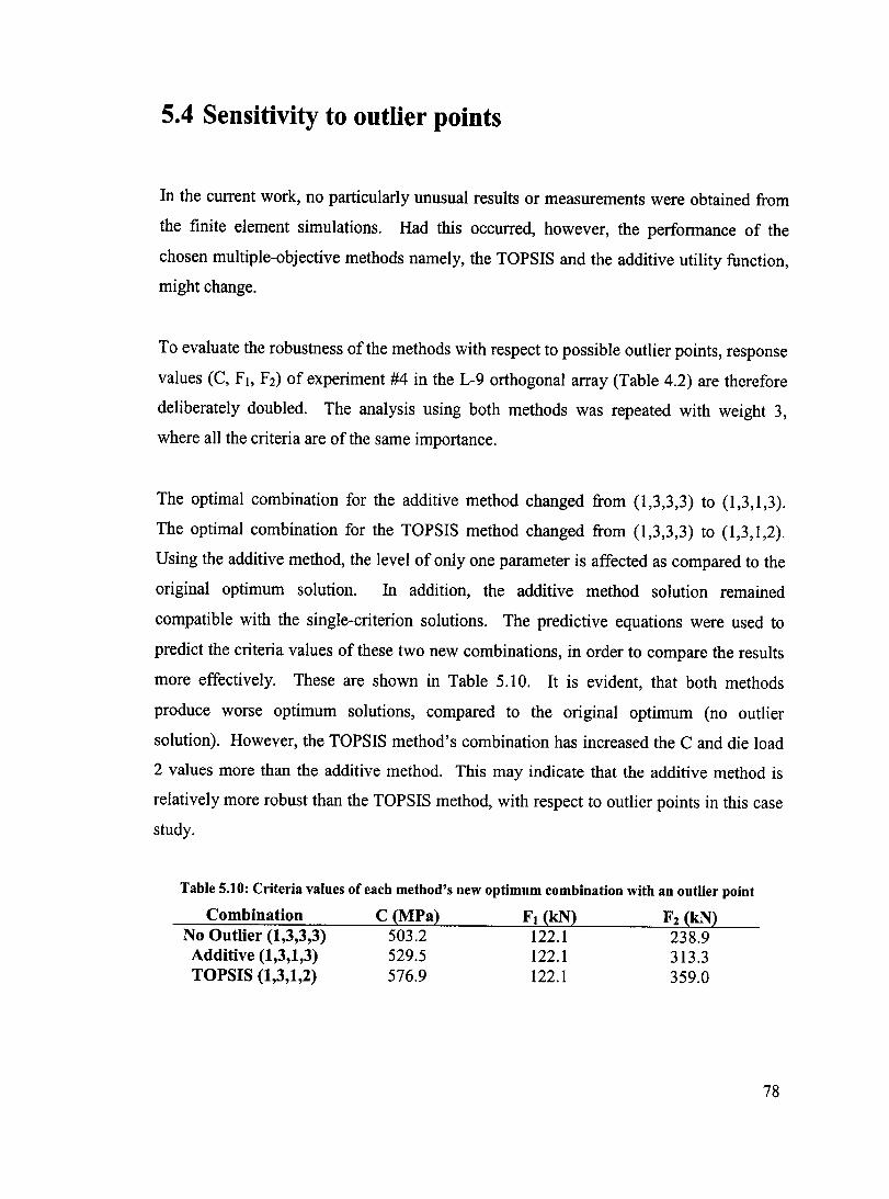
5.4 Sensitivity to outlier points
In the current work, no particularly unusual results or measurements were obtained from
the finite element simulations. Had this occurred, however, the performance of the
chosen multiple-objective methods namely, the TOPSIS and the additive utility function,
might change.
To evaluate the robustness of the methods with respect to possible outlier points, response
values (C, FI, F2) of experiment #4 in the L-9 orthogonal array (Table 4.2) are therefore
deliberately doubled. The analysis using both methods was repeated with weight 3,
where aIl the criteria are of the same importance.
The optimal combination for the additive method changed from (1,3,3,3) to (1,3,1,3).
The optimal combination for the TOPSIS method changed from (1,3,3,3) to (1,3,1,2).
Using the additive method, the level of only one parameter is affected as compared to the
original optimum solution. In addition, the additive method solution remained
compatible with the single-criterion solutions. The predictive equations were used to
predict the criteria values of these two new combinations, in order to compare the results
more effectively. These are shown in Table 5.10. It is evident, that both methods
produce worse optimum solutions, compared to the original optimum (no outlier
solution). However, the TOPSIS method's combination has increased the C and die load
2 values more than the additive method. This may indicate that the additive method is
relatively more robust than the TOPSIS method, with respect to outlier points in this case
study.
Table 5.10: Criteria values of each method's new optimum combination with an outlier point
Combination No Outlier (1,3,3,3) Additive (1,3,1,3) TOPSIS (1,3,1,2)
C (MPa) 503.2 529.5 576.9
FI (kN) 122.1 122.1 122.1
F2 (kN) 238.9 313.3 359.0
78

Conclusions and Future Work
6.1 Conclusions and summary
• The co Id heading process (CHP) is an important manufacturing technique that is
commonly used to produce fasteners, such as bolts, rivets, and nuts.
• Even though it is very widely used, the CHP can produce a number of potential
defects in the formed part. Recently, therefore, much attention has been given to
the design of forming stages.
• In the current work, a simulation of a three-stage cold heading process is
performed using Abaqus Explicit v6.3. The model is axisymmetric, adiabatic,
with 4-noded continuum elements. Constant velocities are applied to rigid dies
which deform a solid blank.
• The blank material is considered to be an elastic-rate-dependant-plastic solid with
the flow stress given by the Johnson-Cook equation. The values of the material
constants are determined by performing quasi-static tension tests on samples of
the material. The st~el is of AIS! 1008 grade. A 1038 steel is also considered but
found to be inadequate for this forming process.
• Potential defects are assessed from the results of the simulations. The Cockroft
and Latham parameter is used for external cracks. The shear band initiation
criterion which states that initiation occurs when thermal softening is greater than
strain and rate hardening is used for internaI cracks. For the formation of shear
bands, criteria that consider the stress drop and temperature rise in a localized
band are used.
79

• A methodology for the optimization of the preform die geometries is introduced.
Two geometrical parameters on each preform die (stages 1 and 2) are given three
level variations. Four parameters, three-Ievel variations gives rise to a total of 82
experiments to be performed. This is reduced to 9 by the Taguchi L-9 orthogonal
array.
• Three criteria are considered for optimization: the Cockroft and Latham
parameter, die load in stage 1 and die load in stage 2. InternaI shear band criteria
are not inc1uded in the optimization because they are found not to vary
significantly with preform geometry.
• The conventional Taguchi approach is applied on mean values, for each criterion.
Additivity of the method is assessed, and the assumption of no interaction
between factors is found to be valid. The ANOV A method is used to determine
the effect of each factor on each response. Three optimal solutions are generated.
Conflicts are found to exist in the solutions of two parameters.
• The conventional Taguchi approach is extended to multiple-criteria approaches by
the use of overall evaluation criteria methods.
• In the MODM method, the utility function is applied on criteria values of each
experiment, in order to first arrive at an OEC index, U, for each experiment. Then
the Taguchi search method is applied on each factor to choose the level of the
factor that minimizes the MODM index. Additive, minimax and multiplicative
functions are analyzed. Six different weights that represent the designer's
preferences among criteria are applied.
• It is found that the additive method is the most adequate for this optimization.
Criteria values for the optimal combinations are plotted to produce Pareto frontier
points. AU points above this frontier are 'dominated' solutions, or solutions that
can be optimized. AIl points below are infeasible.
80
• In the MADM method, the Taguchi approach is first partly applied by averaging
criteria values of each factor leve1, and then the MADM TOPSIS search method is
applied to each factor, to search for that factor's best alternative (level). The best
level is then chosen based on the 'performance' ofits criteria vector. Performance
is defined by the TOPSIS OEC index, CL+. The same weights are applied for this
method.
• The TOPSIS and additive methods are compared. The generated optimal
solutions of the two are identical in most cases. The methods differ only when the
ideal solution is also closest to the nadir solution.
• The additive utility function and TOPSIS methods are also compared for their
sensitivities to outlier points. The additive method may potentially be less
sensitive to such points.
6.2 Future work:
~ Manufacturing tolerances could be included in the analysis. Signal to
noise ratios can then be used in the Taguchi approach, instead of mean values.
~ The following may be further studied:
.:. Different die geometries .
• :. The effect of the number of stages on the likelihood of cracking .
• :. The effect ofheterogeneous strain resulting from extrusion on the
blank before heading.
81
Reference List
Bakhshi-Jooybari M., 1. Pillinger, T. A. Dean and P. Hartley (1996), Development of Product and Process Criteriafor an Intelligent Knowledge-Based System for Forging Die Design, Proceedings of the Institute of Mechanical Engineers, Journal of Engineering Manufacture, vol. 210, p. 565.
Batra R.C. and C.H. Kim (1992), Analysis of Shear Banding in Twelve Materials, International Journal ofPlasticity, vol. 8, p.425.
Behrens A., H. Just, and D. Landgrebe (2000), Prediction of Cracks in Multistage Cold Forging Operations by Finite-Element-Simulations with Integrated Damage Criteria, Proceedings of the International Conference "Metal Forming 2000", Krakow Poland, p. 237.
Brethenoux G., E. Bourgain, G. Piers on, M. Jallon and P. Secordel (1996), Cold Forming Processes: Some Examples of Predictions and Design Optimization using Numerical Simulation, Journal of Materials Processing Technology, vol. 60, p. 555.
Chankong V. and Y. Y. Haimes (1983), Multiobjective Decision Making Theory and Methodology, Elsevier, New York.
Cockroft M.G. and D.J. Latham (1968), Ductility and Workability of Metals, Journal of the Institute of Metals, vol. 96, p. 33.
Deltort B. (1994), Experimental and Numerical Aspects of Adiabatic Shear in a 4340 Steel, Journal de Physique, vol. C 8, p. 447.
Dong-Hyun J. and K. Ki-Ju (2000), A Methodfor Optimal Material Selection Aided with Decision Making Theory, Journal of Materials Design, vol. 21, p. 199.
Fowlkes W.Y., and C. M. Creveling (1995), Engineering Methods for Robust Product Design: Using Taguchi Methods in Technology and Product Development, AddisonWesley, California.
Gokler M. 1., H. Darendehler, N. Elmaskaya (1999), Analysis of Tapered Preforms in Cold Upsetting, International Journal of Machine Tools and Manufacture, vol. 39, p. 1.
Groenbaek J. and Birker T. (2000), Innovations in Cold Forging Die Design, Journal of Materials Processing Technology, vol. 98, p. 155.
Hobbs B. F. (1986), What Can We Learn from Experiments in Multiobjective Decision Analysis?, IEEE Transactions on Systems, Man, and Cybernetics, vol. 16, no. 3, p. 384.
82
Hwang K.-H., K.-W. Lee and G.-J. Park (2001), Robust Optimization of an Automobile Rearview Mirror for Vibration Reduction, Journal of Structural and Multidisciplinary Optimization, vol. 21, p. 300.
lm Y.-T. (1999), A Computer-Aided-Design Systemfor Forming Processes, Journal of Materials Processing Technology, vol. 89, p. 1.
Incropera F. P., D. P. DeWitt (1996), Fundamentals of Heat and Mass Transfer, Wiley, New York.
Janicek L., J. Petruska, B. Maros and S. Rusz (2002), Cold Forming of Bolts Without Thermal Treatment, Journal ofMaterials Processing Technology, vol. 125, p. 341.
Johnson G.R. and W.H. Cook (1983), A Constitutive Model and Data for Metals Subjected to Large Strain Rates and High Temepratures, Proceedings of the 7th International Symposium on Ballistics, Hague, Netherlands, p. 541.
Ko D.-C., D.-H. Kim and B.-M. Kim (1999), Application of Artificial Neural Network and Taguchi Method to Preform Design in Metal Forming Considering Workability, International Journal of Machine Toois and Manufacture, vol. 39, p. 771.
Kunjur A. and S. Krishnamurty (1997), A Robust Multi-Criteria Optimization Approach, Mechanical Machining Theory, vol. 32, no.7, p. 797.
MacCormack C. and J. Monaghan (2002), 2D and 3D Element Analysis of a Three Stage Forging Sequence, Journal of Materials Processing Technology, vol. 58, pp. 1-9.
Meyer H. (1960), Die Marsenverteilung Beim Schmieden in WaagerectStauchmaschinen, Werkstattstechnic, vol. 50, no. 6, p. 333.
Miettinen K. (1999), Nonlinear Multiobjective Optimization, Kluwer Academic, London York.
Milani A.S., A. Shanian, R. Madoliat and J. A. Nemes (2003), The Effect of Normalization Norms in Multiple Attribute Decision Making (MADM) Models: A Case Study in Gear Material Selection, Submitted to Journal of Structural and Multidisciplinary Optimization.
Naujoks W. and D.C. Fabel (1948), Forging Handbook, 4th ed., The American Society for Metals, Cleveland.
Nickoletopoulos N. (2000), Physical and Numerical Modeling of Fracture du ring Upsettingfor Cold Heading Operations, Ph.D. Thesis, McGill University.
Oh S.I., C.c. Chen and S. Kobayashi (1979), Ductile Fracture in Axisymmetric Extrusion and Wire Drawing: Part 2-Workability in Extrusion and Drawing, ASME Journal of Engineering for Industry, vol. 101, no.l, p. 23.
83

Otto K. N and E. K. Antonsson (1993), Extensions to the Taguchi Method ofProduct Design, ASME Journal of Mechanical Design, vol. 115, no. l, p. 5.
Petrescu D., S.C. Savage and P.D. Hodgson (2002), Simulation of the Fastener Manufacturing Process, Journal of Materials Processing Technology, vo1.125-126, p.361.
Roque M. O. L. and S. T. Button (2000), Application of the Finite Element Method in Cold Forging Processes, Journal of the Brazilian Society of Mechanical Sciences, vol. XXII, no.2, p. 189.
Roy B. and V. Mousseau (1996), A Theoretical Frameworkfor Analyzing the Notion of Relative Importance of Criteria, Journal of Multi-Criteria Decision Analysis, vol. 5, no.2, p.145.
Roy S., S. Ghosh, and R. Shivpuri (1997), A New Approach to Optimal Design ofMultistage Forming Pro cesses with Micro Genetic Algorithms, International Journal of Machine Tools and Manufacture, vol. 37, no.l, p. 29.
Roy, R. K. (2001) Design of Experiments Using the Taguchi Approach, Wiley, New York.
Sen P. and J. B. Yang (1998), Multiple Criteria Decision Support in Engineering Design, Springer, New York.
Tong L.-I. and C.-T. Su (1997), Optimizing Multi-Response Problems in The Taguchi Method by Fuzzy Multiple Attribute Decision Making, Quality, Reliability and Engineering International, vol. 13, p. 25.
84
Recommended