ISA-RP67.04-Part II-1994

Approved September 30, 1994

Recommended Practice

Methodologies for the

Determination of Setpoints for

Nuclear Safety-Related

Instrumentation

Second Printing: May 1995

ISA-RP67.04-Part II — Methodologies for the Determination of Setpoints for Nuclear Safety- Related Instrumentation

ISBN: 1-55617-535-3

Copyright 1995 by the Instrument Society of America. All rights reserved. Printed in the UnitedStates of America. No part of this publication may be reproduced, stored in a retrieval system, ortransmitted in any form or by any means (electronic, mechanical, photocopying, recording, orotherwise), without the prior written permission of the publisher.

ISA67 Alexander DriveP.O. Box 12277Research Triangle Park, North Carolina 27709

Preface

This preface is included for informational purposes and is not part of ISA-RP67.04, Part II.

This recommended practice has been prepared as part of the service of ISA, the internationalsociety for measurement and control, toward a goal of uniformity in the field of instrumentation.To be of real value, this document should not be static but should be subject to periodic review.Toward this end, the Society welcomes all comments and criticisms and asks that they beaddressed to the Secretary, Standards and Practices Board; ISA; 67 Alexander Drive; P. O. Box12277; Research Triangle Park, NC 27709; Telephone (919) 549-8411; Fax (919) 549-8288; E-mail: standards@isa.org.

It is the policy of ISA to encourage and welcome the participation of all concerned individuals andinterests in the development of ISA standards, recommended practices, and technical reports.Participation in the ISA standards-making process by an individual member in no way constitutesendorsement by the employer of that individual, of ISA, or of any of the standards that ISAdevelops.

The ISA Standards and Practices Department is aware of the growing need for attention to themetric system of units in general and the International System of Units (SI) in particular, in thepreparation of instrumentation standards, recommended practices, and technical reports.However, since this recommended practice does not provide constants or dimensional values foruse in the manufacture or installation of equipment, English units are used in the examplesprovided.

Before utilizing this recommended practice, it is important that the user understand the relevanceof instrument channel uncertainty and safety-related setpoint determination for nuclear powerplants. Safety-related instrument setpoints are chosen so that potentially unsafe or damagingprocess excursions (transients) can be avoided and/or terminated prior to exceeding safety limits(process-design limits). The selection of a setpoint requires that consideration be given to muchmore than just instrumentation.

Experience has shown that an operational limit should be placed on critical process parametersto ensure that, given the most severe operating or accident transient, the plant's design safetylimits will not be exceeded. Performance of an accident analysis establishes the analytical limitsfor critical process parameters. Typically, the accident analysis models include thethermodynamic, hydraulic, and mechanical dynamic response of the processes as well asassumptions regarding the time response of instrumentation. The analytical limits, as establishedby an accident analysis, do not normally include considerations for the accuracy (uncertainty) ofinstalled instrumentation. To ensure that the actual trip setpoint of an instrument channel isappropriate, additional analysis may be necessary.

Instrument channel uncertainty should be determined, based on the characteristics of installedinstrumentation, the environmental conditions present at the plant locations associated with theinstrumentation, and on process conditions. A properly calculated setpoint will initiate a plantprotective action before the process parameter exceeds its analytical limit, which, inturn, ensuresthat the transient will be avoided and/or terminated before the process parameter exceeds theestablished safety limit.

ISA-S67.04 was initially developed in the middle 1970s by the industry in response to largenumbers of licensee event reports (LER). These LERs were attributed to the lack of adequateconsideration of equipment drift characteristics when establishing the trip setpoints for thelimiting safety system settings (LSSS) and engineered safety features actuation system (ESFAS)

RP67.04, Part II 3

setpoints. These setpoints are included as part of a nuclear power plant's operating license intheir technical specifications. Hence, bistable trip setpoints were found beyond the allowablevalues identified in the technical specifications.

The scope of the standard was focused on LSSS and ESFAS setpoints. As the standard evolved,it continued to focus on those key safety-related setpoints noted previously. It may also be notedthat as the technical specifications have evolved, the values now included in the technicalspecifications may be the trip setpoint or the allowable value or both depending on the setpointmethodology philosophy used by the plant and/or the Nuclear Steam Supply Systems (NSSS)vendor. The methodologies, assumptions, and conservatism associated with performing accidentanalyses and setpoint determinations, like other nuclear power plant technologies, have alsoevolved. This evolution has resulted in the present preference for explicit evaluation of instrumentchannel uncertainties and resulting setpoints rather than implicitly incorporating suchuncertainties into the overall safety analyses. Both the explicit and implicit approaches canachieve the same objective of assuring that design safety limits will not be exceeded. During theprocess of developing the 1988 revision of ISA-S67.04, it was determined that, because of theevolving expectations concerning setpoint documentation, additional guidance was neededconcerning methods for implementing the requirements of the standard. In order to address thisneed, standard Committees SP67.15 and SP67.04 were formed and have prepared thisrecommended practice. It is the intent of the Committees that the scope of the recommendedpractice be consistant with the scope of the standard. The recommended practice is to be utilizedin conjunction with the standard. The standard is 67.04, Part I, and the recommended practice is67.04, Part II.

During the development of this recommended practice, a level of expectation for setpointcalculations has been identified, which, in the absence of any information on application to lesscritical setpoints, leads some users to come to expect that all setpoint calculations will contain thesame level of rigor and detail. The lack of specific treatment of less critical setpoints has resultedin some potential users expecting the same detailed explicit consideration of all the uncertaintyfactors described in the recommended practice for all setpoints. It is not the intent of therecommended practice to suggest that the methodology described is applicable to all setpoints.Although it may be used for most setpoint calculations, it is by no means necessary that it may beused for all setpoints. In fact, in some cases, it may not be appropriate.

Setpoints associated with the analytical limits determined from the accident analyses areconsidered part of the plant's safety-related design since they are critical to ensuring the integrityof the multiple barriers to the release of fission products. This class of setpoints and theirdetermination have historically been the focus of ISA-S67.04 as discussed above.

Also treated as part of many plants' safety-related designs are setpoints that are not determinedfrom the accident analyses and are not required to maintain the integrity of the fission productbarriers. These setpoints may provide anticipatory inputs to, or reside in, the reactor protection orengineered safeguards initiation functions but are not credited in any accident analysis.Alternatively, there are setpoints that support operation of, not initiation of, the engineered safetyfeatures.

In applying the standard to the determination of setpoints, a graduated or "graded" approach maybe appropriate for setpoints that are not credited in the accident analyses to initiate reactorshutdown or the engineered safety features.

While it is the intent that the recommended practice will provide a basis for consistency inapproach and terminology to the determination of setpoint uncertainty, it is acknowledged thatthe recommended practice is not an all-inclusive document. Other standards exist that containprinciples and terminology, which, under certain circumstances, may be useful in estimatinginstrument uncertainty. It is acknowledged therefore that concerns exist as to whether therecommended practice is complete in its presentation of acceptable methods. The user is

4 RP67.04, Part II

encouraged to review several of the references in the recommended practice that contain otherprinciples and terminology.

The uncertainty and setpoint calculations discussed in this recommended practice may beprepared either manually or with a computer software program. The documentation associatedwith these calculations is discussed in Section 10; however, the design control anddocumentation requirements of manual calculations or computer software are outside the scopeof the recommended practice.

This recommended practice is intended for use primarily by the owners/operating companies ofnuclear power plant facilities or their agents (NSSS, architects, engineers, etc.) in establishingsetpoint methodology programs and preparing safety-related instrument setpoint calculations.

This recommended practice utilizes statistical nomenclature that is customary and familiar topersonnel responsible for nuclear power plant setpoint calculations and instrument channeluncertainty evaluation. It should be noted that this nomenclature may have different definitions inother statistical applications and is not universal, nor is it intended to be. Furthermore, in keepingwith the conservative philosophy employed in power plants calculations, the combination ofuncertainty methodology for both dependent and independent uncertainty components isintended to be bounding. That is, the resultant uncertainty should be correct or overlyconservative to ensure safe operation. In cases where precise estimation of measurementuncertainty is required, more sophisticated techniques should be employed.

ISA Standard Committee SP67.04 operates as a Subcommittee under SP67, the ISA NuclearPower Plant Standards Committee, with H. R. Wiegle as Chairman.

The following people served as members of ISA Subcommittees SP67.04 and SP67.15, whichwas incorporated into SP67.04:

NAME COMPANY

*R. George, Chairman 67.04 PECO Energy CompanyB. Beuchel, Chairman 67.15 NAESCO

*T. Hurst, Vice Chairman 67.04 Hurst ConsultingM. Widmeyer, Managing Director The Supply System

*J. Adams Omaha Public Power DistrictM. Adler Volian EnterprisesD. Alexander Detroit Edison CompanyR. Allen ABB Combustion Engineering, Inc.

*J. Alvis ABB Impell InternationalM. Annon I&C Engineering Associates

*J. Arpin Combustion Engineering, Inc.*J. Ashcraft Tenera*B. Basu Southern California Edison CompanyL. Bates Portland General Electric CompanyM. Belew Tennessee Valley AuthorityF. Berté Tetra Engineering Group, Inc.P. Blanch Consultant

*R. Bockhorst Southern California Edison CompanyR. Brehm Tennessee Valley AuthorityW. Brown ISD CorporationR. Burnham ConsultantM. Burns Arizona Public Service

* One vote per company

RP67.04, Part II 5

NAME COMPANY

T. Burton INPO*G. Butera Baltimore Gas & ElectricR. Calvert Consultant

*J. Carolan PECO Energy Company*J. Cash Tenera*G. Chambers Southern California Edison CompanyR. Chan Salem/Hope Creek Generating Station

*G. Cooper Commonwealth EdisonL. Costello Carolina Power & Light Company

*W. Cottingham Entergy Operations, Inc.C. Cristallo, Jr. Northeast UtilitiesW. Croft Westinghouse Electric Corporation

*W. Crumbacker Sargent & Lundy Engineers*J. Das Ebasco Services, Inc.*J. DeMarco Sargent & LundyD. Desai Consolidated Edison of New York, Inc.T. Donat ConsultantC. Doyel Florida Power Corporation

*M. Durr New York Power AuthorityM. Eidson Southern Nuclear Operating Company

*R. Ennis TeneraS. Eschbach B&W Advanced Systems Engineering

*R. Estes Hurst ConsultingR. Fain Analysis & Measurement ServicesR. Fredricksen New York Power AuthorityV. Fregonese Carolina Power & Light CompanyD. Gantt Westinghouse Hanford CompanyS. Ghbein Washington PPSS

*R. Givan Sargent & Lundy*W. Gordon Bechtel CompanyR. Gotcher Weed Instrument Company

*R. Hakeem Gulf States UtilitiesR. Hardin Catawba Nuclear SiteB. Haynes SAIC

*K. Herman Pacific Gas & Electric Company*J. Hill Northern States Power Company*W. Hinton Entergy Operations, Inc.P. Holzman Star, Inc.

*D. Howard Ebasco Services*E. Hubner Stone & Webster*P. Hung Combustion EngineeringK. Iepson Iepson Consulting Enterprise, Inc.

*J. James Stone & Webster, Inc.S. Jannetty Proto-Power EngineeringJ. Kealy ConsultantJ. Kiely Northern States Power

*S. Kincaid Hurst Engineering, Inc.*W. Kramer Westinghouse Electric Corporation

* One vote per company

6 RP67.04, Part II

NAME COMPANY

*T. Kulaga Ebasco Services, Inc.*L. Lemons Pacific Gas & Electric CompanyJ. Leong General Electric Company

*L. Lester Omaha Public Power District*P. Loeser U.S. Nuclear Regulatory Commission*J. Long Bechtel CompanyK. Lyall Duke Power Company

*J. Mauck U.S. Nuclear Regulatory CommissionI. Mazza Trasferimento di TecnologieW. McBride Virginia PowerB. McMillen Nebraska Public Power District

*C. McNall Tenera*D. McQuade Combustion Engineering*J. McQuighan Baltimore Gas & Electric CompanyD. Miller Ohio State University

*J. Mock Bechtel CompanyU. Mondal Ontario HydroR. Morrison TU Electric - CPSES

*R. Naylor Commonwealth EdisonR. Neustadter Raytheon Engineers & Constructors, Inc.

*J. O'Connell ABB Impell CorporationJ. Osborne Florida State & Light CompanyJ. Peternel SOR, Inc.

*A. Petrenko New York Power Authority*K. Pitilli ABB Impell Corporation*R. Plotnick Stone & Webster Corporation*B. Powell MDM EngineeringR. Profeta S. Levy, Inc.B. Queenan VectraT. Quigley Northeast Utilities

*E. Quinn MDM EngineeringS. Rabinovich ConsultantD. Rahn Signals & Safeguards, Inc.

*T. Reynolds Weed InstrumentD. Ringland Foxboro CompanyS. Roberson Onsite Engineering & Management

*D. Sandlin Gulf States UtilitiesJ. Sandstrom Rosemount, Inc.

*R. Sawaya Northern States Power CompanyJ. Scheetz Pacific Engineering Corporation

*R. Schimpf New York Power AuthorityR. Schwartzbeck Enercon Services, Inc.F. Semper Semper EngineeringJ. Shank Carolina Power & Light CompanyT. Slavic Duquesne Light CompanyC. Sorensen Southern Company ServicesW. Sotos American Electric Power Service Corporation

*R. Szoch, Jr. Baltimore Gas & Electric Company

* One vote per company

RP67.04, Part II 7

NAME COMPANY

B. Sun Electric Power Research InstituteR. Tanney Cleveland IlluminatingW. Trenholme Arizona Public Service

*C. Tuley Westinghouse Electric CorporationP. VandeVisse Consultant

*T. Verbout Northern States Power CompanyJ. Voss Tenera LPJ. Wallace Wisconsin Public ServiceR. Webb Pacific Gas & Electric Company

*S. Weldon Hurst Engineering, Inc.R. Westerhoff Consumers Power Company

*P. Wicyk Commonwealth Edison*R. Wiegle Philadelphia Electric CompanyV. Willems Gilbert Commonwealth

*G. Wood Entergy Operations, Inc. - Waterford 3B. Woodruff Florida Power & Light Company

The following people served as members of ISA Committee SP67:

NAME COMPANY

H. Wiegle, Chairman PECO Energy CompanyW. Sotos, Vice Chairman American Electric Power Service CorporationM. Widmeyer, Managing Director The Supply SystemR. Allen Combustion Engineering, Inc.M. Annon I&C Engineering Associates

*B. Basu Southern California Edison CompanyJ. Bauer General Atomics CompanyM. Belew Tennessee Valley AuthorityM. Berkovich Bechtel Power CorporationB. Beuchel NAESCOP. Blanch ConsultantT. Burton INPO

*G. Cooper Commonwealth EdisonN. Dogra Impell Corporation

*A. Ellis Westinghouse Electric CorporationR. Estes Hurst Engineering, Inc.H. Evans Pyco, Inc.V. Fregonese Public Service Electric & GasR. George PECO Energy Company

*R. Givan Sargent & Lundy*W. Gordon Bechtel Savannah River, Inc.R. Gotcher Weed Instrument CompanyT. Grochowski UNC Engineering Services, Inc.

*S. Hedden Commonwealth Edison K. Herman Pacific Gas & Electric Company

*R. Hindia Sargent & Lundy

* One vote per company

8 RP67.04, Part II

NAME COMPANY

E. Hubner Stone & WebsterJ. Lipka Consultant

*P. Loeser US Nuclear Regulatory Commission*J. Mauck US Nuclear Regulatory CommissionB. McMillen Nebraska Public Power DistrictL. McNeil INPOA. Machiels Electric Power Research InstituteG. Minor MHB Technical Association

*J. Mock Bechtel Company*J. Nay Westinghouse Electric Corporation*R. Naylor Commonwealth EdisonR. Neustadter Raytheon Engineers & Constructors, Inc.R. Profeta S. Levy, Inc.

*J. Redmon Southern California Edison CompanyA. Schager ConsultantF. Semper Semper Engineering

*T. Slavic Duquesne Light CompanyI. Smith AEA TechnologyW. Sotos American Electric Power Service CorporationI. Sturman Bechtel CompanyW. Trenholme I&C ConsultantC. Tuley Westinghouse Electric CorporationK. Utsumi General Electric CompanyR. Webb Pacific Gas & Electric Company

*G. Whitmore Duquesne Light CompanyP. Wicyk Commonwealth Edison CompanyF. Zikas Parker-Hannifin Corporation

This published standard was approved for publication by the ISA Standards and Practices Board in September 1994.

NAME COMPANY

W. Weidman, Vice President Gilbert Commonwealth, Inc.H. Baumann H. D. Baumann & Associates, Ltd.D. Bishop Chevron USA Production CompanyW. Calder III Foxboro CompanyC. Gross Dow Chemical CompanyH. Hopkins Utility Products of ArizonaA. Iverson Lyondell Petrochemical CompanyK. Lindner Endress + Hauser GmbH + CompanyT. McAvinew Metro Wastewater Reclamation DistrictA. McCauley, Jr. Chagrin Valley Controls, Inc.G. McFarland ABB Power Plant ControlsJ. Mock Bechtel CompanyE. Montgomery Fluor Daniel, Inc.D. Rapley Rapley Engineering Services

* One vote per company

RP67.04, Part II 9

NAME COMPANY

R. Reimer Allen-Bradley CompanyR. Webb Pacific Gas & Electric CompanyJ. Weiss Electric Power Research InstituteJ. Whetstone National Institute of Standards & TechnologyM. Widmeyer The Supply SystemC. Williams Eastman Kodak CompanyG. Wood Graeme Wood ConsultingM. Zielinski Fisher-Rosemount

10 RP67.04, Part II

Contents

1 Scope ..................................................................................................................................... 13

2 Purpose .................................................................................................................................. 13

3 Definitions ............................................................................................................................. 13

4 Using this recommended practice ...................................................................................... 16

5 Preparation for determining instrument channel setpoints ............................................. 17

5.1 Diagramming instrument channel layout ................................................................ 175.2 Identifying design parameters and sources of uncertainty ................................... 19

6 Calculating instrument channel uncertainties ................................................................... 22

6.1 Uncertainty equations ............................................................................................... 226.2 Uncertainty data ........................................................................................................ 256.3 Calculating total channel uncertainty ...................................................................... 38

7 Establishment of setpoints .................................................................................................. 45

7.1 Setpoint relationships ............................................................................................... 457.2 Trip setpoint determination ...................................................................................... 467.3 Allowable value .......................................................................................................... 47

8 Other considerations ............................................................................................................ 48

8.1 Correction for setpoints with a single side of interest ........................................... 49

9 Interfaces .............................................................................................................................. 49

10 Documentation .................................................................................................................... 51

11 References ........................................................................................................................... 52

11.1 References used in text .......................................................................................... 5211.2 Informative references ............................................................................................ 54

Appendices

A: Glossary ............................................................................................................................... 57

B: Vessel/reference leg temperature effects on differential pressure transmitters used for level measurement ......................................................................... 61

C: Effects on flow measurement accuracy ............................................................................ 69

D: Insulation resistance effects .............................................................................................. 73

E: Plant specific as found/as left data ................................................................................... 81

F: Line pressure loss/head pressure e ffects ......................................................................... 85

RP67.04, Part II 11

G: RTD accuracy confirmation ............................................................................................... 87

H: Uncertainties associated with digital signal processing ................................................. 89

I : Recommendations for inclusion of instrument uncertainties during normal operation in the allowable value determination ................................................... 93

J: Discussions concerning statistical analysis ..................................................................... 95

K: Propagation of uncertainty through signal conditioning modules ................................ 97

L: Example of uncertainty/setpoint calculations ................................................................ 103

1 Example calculation - Pressure trip .......................................................................... 1052 Example calculation - Flow trip ................................................................................. 1153 Example calculation - Level trip ................................................................................ 1274 Example calculation - Radiation trip ......................................................................... 143

12 RP67.04, Part II

1 Scope

This recommended practice provides guidance for the implementation of ISA-S67.04, Part I inthe following areas:

a) Methodologies, including sample equations to calculate total channel uncertainty

b) Common assumptions and practices in instrument uncertainty calculations

c) Equations for estimating uncertainties for commonly used analog and digital modules

d) Methods to determine the impact of commonly encountered effects on instrument uncertainty

e) Application of instrument channel uncertainty in setpoint determination

f) Sources and interpretation of data for uncertainty calculations

g) Discussion of the interface between setpoint determination and plant operating procedures, calibration procedures, and accident analysis

h) Documentation requirements

2 Purpose

The purpose of this recommended practice is to present guidelines and examples of methods forthe implementation of ISA-S67.04, Part I in order to facilitate the performance of instrumentuncertainty calculations and setpoint determination for safety-related instrument setpoints innuclear power plants.

3 Definitions

3.1 allowable value: A limiting value that the trip setpoint may have when tested periodically, beyond which appropriate action shall be taken.

3.2 analytical limit: Limit of a measured or calculated variable established by the safety analysis to ensure that a safety limit is not exceeded.

3.3 abnormally distributed uncertainty: A term used in this recommended practice to denote uncertainties that do not have a normal distribution. See 6.2.1.2.2 for further information.

RP67.04, Part II 13

3.4 as found: The condition in which a channel, or portion of a channel, is found after a period of operations and before recalibration (if necessary).

3.5 as-left: The condition in which a channel, or portion of a channel, is left after calibration or final setpoint device setpoint verification.

3.6 bias: An uncertainty component that consistently has the same algebraic sign and is ex-pressed as an estimated limit of error.

3.7 bistable :1 A device that changes state when a preselected signal value is reached.

3.8 dependent uncertainty: Uncertainty components are dependent on each other if they possess a significant correlation, for whatever cause, known or unknown. Typically, dependencies form when effects share a common cause.

3.9 drift: An undesired change in output over a period of time where change is unrelated to the input, environment, or load.

3.10 effect: A change in output produced by some outside phenomena, such as elevated tem-perature, pressure, humidity, or radiation.

3.11 error: The algebraic difference between the indication and the ideal value of the measured signal.

3.12 final setpoint device: A component or assembly of components, that provides input to the process voting logic for actuated equipment. (See IEEE Standard 603.)

NOTE: Examples of final actuation devices are bistables, relays, pressure switches, and level switches.

3.13 independent uncertainty: Uncertainty components are independent of each other if their magnitudes or algebraic signs are not significantly correlated.

3.14 instrument channel: An arrangement of components and modules as required to generate a single protective action signal when required by a plant condition. A channel loses its identity where single protective action signals are combined. (See IEEE Standard 603.)

3.15 instrument range: The region between the limits within which a quantity is measured, received, or transmitted, expressed by stating the lower and upper range values.

3.16 limiting safety system setting (LSSS): Limiting safety system settings for nuclear reactors are settings for automatic protective devices related to those variables having significant safety functions. (See CFR Reference.)

3.17 margin: In setpoint determination, an allowance added to the instrument channel uncertainty. Margin moves the setpoint farther away from the analytical limit.

3.18 module: Any assembly of interconnected components that constitutes an identifiable device, instrument, or piece of equipment. A module can be removed as a unit and replaced with a spare. It has definable performance characteristics that permit it to be tested as a unit. A module can be a card, a drawout circuit breaker, or other subassembly of a larger device, provided it meets the requirements of this definition. (See IEEE Standard 603.)

1 As an example of the intended use of the term "bistable" in the context of this document, electronic trip units in BWRs are considered "bistables."

14 RP67.04, Part II

3.19 nuclear safety-related instrumentat ion: That which is essential to the following:

a) Provide emergency reactor shutdown

b) Provide containment isolation

c) Provide reactor core cooling

d) Provide for containment or reactor heat removal, or

e) Prevent or mitigate a significant release of radioactive material to the environment; or is otherwise essential to provide reasonable assurance that a nuclear power plant can be operated without undo risk to the health and safety of the public.

3.20 primary element: The system element that quantitatively converts the measured variable energy into a form suitable for measurement.

3.21 process measurement instrumentation: An instrument, or group of instruments, that converts a physical process parameter such as temperature, pressure, etc., to a usable, measur-able parameter such as current, voltage, etc.

3.22 random: 2 Describing a variable whose value at a particular future instant cannot be pre-dicted exactly but can only be estimated by a probability distribution function. (See ANSI C85.1.)

3.23 reference accuracy (also known as "accuracy rat ing" as defined in ISA-S51.1): A number or quantity that defines a limit that errors will not exceed when a device is used under specified operating conditions.

3.24 safety limit: A limit on an important process variable that is necessary to reasonably protect the integrity of physical barriers that guard against uncontrolled release of radioactivity. (See CFR Reference.)

3.25 sensor: The portion of an instrument channel that responds to changes in a plant variable or condition and converts the measured process variable into a signal; e.g., electric or pneumatic. (See IEEE Standard 603.)

3.26 signal conditioning: One or more modules that perform signal conversion, buffering, iso-lation, or mathematical operations on the signal as needed.

3.27 signal interface: The physical means (cable, connectors, etc.) by which the process signal is.

3.28 span: The algebraic difference between the upper and lower values of a calibrated range.

3.29 test interval: The elapsed time between the initiation (or successful completion) of tests on the same sensor, channel, load group, safety group, safety system, or other specified system or device. (See ANSI C85.1.)

3.30 tolerance: The allowable variation from a specified or true value. (See IEEE Standard 498.)

3.31 trip setpoint: A predetermined value for actuation of the final actuation device to initiate protective action.

2 In the context of this document, "random" is an abbreviation for random, approximately normally distributed. The algebraic sign of a random uncertainty is equally likely to be positive or negative with respect to some median value. Thus, random uncertainties are eligible for square-root-sum-of-squares combination propagated from the process measurement module through the signal conditioning module of the instrument channel to the module that initiates the actuation.

RP67.04, Part II 15

3.32 uncertainty: The amount to which an instrument channel's output is in doubt (or the allow-ance made therefore) due to possible errors, either random or systematic, that have not been corrected for. The uncertainty is generally identified within a probability and confidence level.

Additional definitions related to setpoints or instrument terminology and uncertainty may be foundin ANSI/ISA-S37.1-1975, ANSI/ISA-S51.1-1979, and ISA-S67.04, Part I-1994.

4 Using this recommended practice

The recommended practice is primarily focused on calculating a setpoint for a single instrumentchannel using acceptable statistical methods, where use of these methods is important toassuring the plant operates within the envelope of the accident analyses and maintains theintegrity of the fission product release barriers. There are a number of different approaches thatare acceptable for use in establishing nuclear safety-related setpoints. The statistical methodpresented in the recommended practice is the most common approach in use at this time. Therecommended practice is intended to identify areas that should be evaluated when one does asetpoint calculation, to present some examples of present thinking in the area of setpointcalculations, and to provide some recommendations for a setpoint methodology. The methodsdiscussed in the recommended practice are not intended to be all-inclusive. The recommendedpractice includes many terms used in probability and statistics. Since it is not the purpose of therecommended practice to be a text on these subjects, it is recommended that the user review atext on statistics to establish a knowledge of some of the terminology in conjunction with the useof the recommended practice.

Additionally, it is recognized that some safety-related setpoints are not tied to the safety analysesand do not, even from a system's standpoint, have an explicit limiting value. Thus a gradedapproach may be applied to the plant's safety-related setpoints. A graded approach might includea method of classifying setpoints according to their contribution to plant safety. Based on themethod of classification, the approach would provide guidance on the method to be used todetermine the channel uncertainty. Specific criteria for establishing a graded approach or thelevel of analysis used as part of this type of approach are outside the scope of the recommendedpractice. For an example of a graded approach, see the R.C. Webb Reference.

The remainder of the recommended practice is structured to mimic the process one would followto determine an instrument channel setpoint. A method for calculating instrument channeluncertainties is discussed in Section 5, and a method for calculating the trip setpoint when onehas analytical limit for the process is discussed in Section 6.

The recommended practice starts in Section 5 with the preparation of a block diagram of theinstrument channel being analyzed. Uncertainty equations and discussions on sources ofuncertainty and interpretation of uncertainty data are presented in 6.1 and 6.2. The basicequations for calculating total instrument channel uncertainty are presented in 6.3. Methods todetermine the instrument channel allowable value and trip setpoint for an instrument channel arepresented in Section 7. Selected subjects related to determining setpoints for nuclear plantinstrumentation are discussed in Section 8.

It is prudent to evaluate setpoint calculations to assure they are not overly conservative. Overlyconservative setpoints can be restrictive to plant operation or may reduce safety byunnecessarily increasing the frequency of safety system actuation. The evaluation should assurethat there are no overlapping, redundant, or inconsistent values or assumptions. Conservatism

16 RP67.04, Part II

may result from the many interfaces between organizations that can have an input to thecalculation. These interfaces are discussed in Section 9.

Documentation considerations are discussed in Section 10. The appendices provide in-depthdiscussions concerning the theory and background for the information presented in Sections 5through 7, as well as extensive and comprehensive examples of setpoint calculations anddiscussions of unique topics in setpoint determination.

5 Preparation for determining instrument channel setpoints

The following discussion provides a suggested sequence of steps to be performed whendeveloping an instrument channel uncertainty or setpoint analysis. The intent is to guide thereader through the basics of the channel layout, functions provided, sources of uncertainty thatmay be present, etc., with references to the appropriate section(s) for detailed discussions ofparticular topics of interest.

5.1 Diagramming instrument channel layout

When preparing an uncertainty or setpoint calculation, it is helpful to generate a diagram of theinstrument channel being analyzed in a manner similar to that shown in Figure 1. A diagram aidsin developing the analysis, classifying the uncertainties that may be present in each portion of theinstrument channel, determining the environmental parameters to which each portion of theinstrument channel may be exposed, and identifying the appropriate module transfer function.

Figure 1 shows a typical instrument channel that could be used to provide a nuclear safety-related protection function. It also shows interfaces, functions, sources of error, and differentenvironments.

RP67.04, Part II 17

Figure 1. Typical instrument channel layout

18 RP67.04, Part II

A typical instrument channel consists of the following major sections:

a) Process

b) Process interface

c) Process measurement

d) Signal interface

e) Signal conditioning

f) Actuation

5.2 Identifying design parameters and sources of uncertainty

The functional requirements, actuation functions, and operating times of the instrument channel,as well as the postulated environments that the instrument could be exposed to concurrent withthese actuations, should be identified. Many times the instrument channel uncertainty isdependent on a particular system operating mode, operating point (i.e., maximum level, minimumflow, etc.), or a particular sequence of events. A caution that should be considered when thesame setpoint is used for more than one actuation function, each with possibly differentenvironmental assumptions, is that the function with the most limiting environmental conditionsshould be used. Where a single instrument channel has several setpoints, either the most limitingset of conditions should be used or individual calculations for each setpoint should be performed,each with the appropriate set of conditions.

Environmental boundaries can then be drawn for the instrument channel as shown in Figure 1.For simplicity, two sets of environmental conditions are shown. Typically, the process measure-ment, process interface, some of the signal conditioning (if applicable), and some of the signalinterface components are located in areas of the plant that may have a significantly different localenvironment from the remainder of the instrument channel. Typically, most signal conditioningcomponents and other electronics are located in a controlled environment not subject tosignificant variations in temperature or to post-accident environments. Therefore, two sets ofenvironmental conditions are defined, with conditions in Environment A normally more harshthan conditions in Environment B. Normally, larger environmental uncertainty allowances will beused with those portions of the instrument channel exposed to Environment A. Environmentaleffects and assumptions pertaining to environmental conditions are discussed in 6.2.4.

After the environmental conditions are determined, the potential uncertainties affecting eachportion of the instrument channel should be determined. For example, the process interfaceportion is normally affected only by process measurement effects and not by equipmentcalibration or other uncertainties. Also, cables in the mild conditions of Environment B would notbe appreciably affected by insulation resistance (IR) effects.

Figure 1 shows where each major class of uncertainty typically will be present. Each major classis listed below along with a further breakdown into particular types and the particular section(s)where each is discussed in the recommended practice. This list is not meant to be all-inclusive.

Process measurement effects

• Vessel/reference leg temperature effects (Appendix B)• Fluid density effects on flow measurement (Appendix C)• Piping configuration effects on flow measurement (Appendix C)• Line pressure loss/head pressure effects (Appendix F)

RP67.04, Part II 19

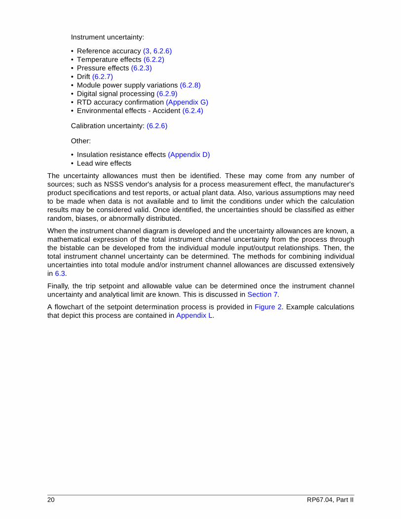
Instrument uncertainty:

• Reference accuracy (3, 6.2.6)• Temperature effects (6.2.2)• Pressure effects (6.2.3)• Drift (6.2.7)• Module power supply variations (6.2.8)• Digital signal processing (6.2.9)• RTD accuracy confirmation (Appendix G)• Environmental effects - Accident (6.2.4)

Calibration uncertainty: (6.2.6)

Other:

• Insulation resistance effects (Appendix D)• Lead wire effects

The uncertainty allowances must then be identified. These may come from any number ofsources; such as NSSS vendor's analysis for a process measurement effect, the manufacturer'sproduct specifications and test reports, or actual plant data. Also, various assumptions may needto be made when data is not available and to limit the conditions under which the calculationresults may be considered valid. Once identified, the uncertainties should be classified as eitherrandom, biases, or abnormally distributed.

When the instrument channel diagram is developed and the uncertainty allowances are known, amathematical expression of the total instrument channel uncertainty from the process throughthe bistable can be developed from the individual module input/output relationships. Then, thetotal instrument channel uncertainty can be determined. The methods for combining individualuncertainties into total module and/or instrument channel allowances are discussed extensivelyin 6.3.

Finally, the trip setpoint and allowable value can be determined once the instrument channeluncertainty and analytical limit are known. This is discussed in Section 7.

A flowchart of the setpoint determination process is provided in Figure 2. Example calculationsthat depict this process are contained in Appendix L.

20 RP67.04, Part II

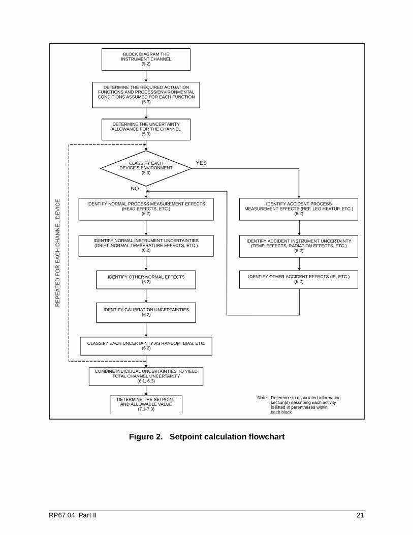
Figure 2. Setpoint calculation flowchart

BLOCK DIAGRAM THEINSTRUMENT CHANNEL

(5.2)

DETERMINE THE UNCERTAINTYALLOWANCE FOR THE CHANNEL

(5.3)

IDENTIFY NORMAL PROCESS MEASUREMENT EFFECTS(HEAD EFFECTS, ETC.)

(6.2)

IDENTIFY ACCIDENT PROCESSMEASUREMENT EFFECTS (REF. LEG HEATUP, ETC.)

(6.2)

IDENTIFY ACCIDENT INSTRUMENT UNCERTAINTY(TEMP. EFFECTS, RADIATION EFFECTS, ETC.)

(6.2)

IDENTIFY OTHER ACCIDENT EFFECTS (IR, ETC.)(6.2)

IDENTIFY NORMAL INSTRUMENT UNCERTAINTIES(DRIFT, NORMAL TEMPERATURE EFFECTS, ETC.)

(6.2)

IDENTIFY OTHER NORMAL EFFECTS(6.2)

IDENTIFY CALIBRATION UNCERTAINTIES(6.2)

CLASSIFY EACH UNCERTAINTY AS RANDOM, BIAS, ETC.(6.2)

COMBINE INDICIDUAL UNCERTAINTIES TO YIELDTOTAL CHANNEL UNCERTAINTY

(6.1, 6.3)

DETERMINE THE SETPOINTAND ALLOWABLE VALUE

(7.1-7.3)

Note: Reference to associated informationsection(s) describing each activityis listed in parentheses withineach block

CLASSIFY EACHDEVICE'S ENVIRONMENT

(5.3)

YES

NO

DETERMINE THE REQUIRED ACTUATIONFUNCTIONS AND PROCESS/ENVIRONMENTALCONDITIONS ASSUMED FOR EACH FUNCTION

(5.3)

RP67.04, Part II 21

6 Calculating instrument channel uncertainties

6.1 Uncertainty equations

Since all measurements are imperfect attempts to ascertain an exact natural condition, the actualmagnitude of the quantity can never be known. Therefore, the actual value of the error in themeasurement of a quantity is also unknown. The amount of the error should therefore bediscussed only in terms of probabilities; i.e., there may be one probability that a measurement iscorrect to within a certain specified amount and another probability for correctness to withinanother specified amount. For the purpose of this recommended practice, the term "uncertainty"will be utilized to reflect the distribution of possible errors.

There are a number of recognized methods for combining instrumentation uncertainties. Themethod discussed by this recommended practice is a combination of statistical and algebraicmethods that uses statistical square root sum of squares (SRSS) methods to combine randomuncertainties and then algebraically combine the nonrandom terms with the result. The formulasand discussion below present the basic principles of this methodology. Another recognizedmethodology to estimate instrument measurement uncertainty is described in ANSI/ASME PTC 19.1. Additional discussion of this methodology is provided in J.1 of Appendix J.

The basic formula for uncertainty calculation takes the form:

Z = +[(A2 + B2 + C2)]1/2 + |F| + L - M (Eq. 6.1)

where

A,B,C = random and independent terms. The terms are zero-centered,approximately normally distributed, and indicated by a ± sign.

F = abnormally distributed uncertainties and/or biases (unknown sign). Theterm is used to represent limits of error associated with uncertainties thatare not normally distributed and do not have known direction. Themagnitude of this term (absolute value) is assumed to contribute to the totaluncertainty in a worst-case direction and is also indicated by a + sign.

L & M = biases with known sign. The terms can impact an uncertainty in aspecific direction and, therefore, have a specific + or - contribution to thetotal uncertainty.

Z = resultant uncertainty. The resultant uncertainty combines the randomuncertainty with the positive and negative components of the nonrandomterms separately to give a final uncertainty. The positive and negativenonrandom terms are not algebraically combined before combination withthe random component.

22 RP67.04, Part II

The addition of the F, L, and M terms to the A, B, and C uncertainty terms allows the formula toaccount for influences on total uncertainty that are not random or independent. For biases withknown direction, represented by L and M, the terms are combined with only the applicableportion (+ or -) of the random uncertainty. For the uncertainty represented by F, the terms arecombined with both portions of the random uncertainty. Since these terms are uncertaintiesthemselves, the positive and negative components of the terms cannot be algebraicallycombined into a single term. The positive terms of the nonrandom uncertainties should besummed separately, and the negative terms of the nonrandom uncertainties should be summedseparately and then individually combined with the random uncertainty to yield a final value.Individual nonrandom uncertainties are independent probabilities and may not be presentsimultaneously. Therefore, the individual terms cannot be assumed to offset each other3.

If R equals the resultant random uncertainty (A2 + B2 + C2)1/2, the maximum positive uncertaintyis

+Z = +R + |F| + L

and the maximum negative uncertainty is

-Z = -R - |F| - M

SRSS combination for bias uncertainties is inappropriate since by their nature, they do not satisfythe prerequisites for SRSS. Bias uncertainties are not random and are not characterized by anormal probability distribution. Since the number of known biases is typically small and they mayor may not be present simultaneously, the recommended practice conservatively endorsesalgebraic summation for bias uncertainties.

In the determination of the random portion of an uncertainty, situations may arise where two ormore random terms are not totally independent of each other but are independent of the otherrandom terms. This dependent relationship can be accommodated within the SRSS methodologyby algebraically summing the dependent random terms prior to performing the SRSSdetermination. The formula takes the following form:

Z = + [A2 + B2 + C2 + (D + E)2]1/2 + |F| + L - M (Eq. 6.2)

where

D and E = random dependent uncertainty terms that are independent of Terms A, B, and C.

The uncertainty terms of Equation 6.2 and their associated relationships are depicted in Figure 3.

3 The purpose of the setpoint calculation is to ensure that protective actions occur 95 percent of the time with a high degree of confidence before the analytical limits are reached. A conservative philosophy applies the SRSS technique only to those uncertainties that are characterized as independent, random, and approximately normally distributed (or otherwise allowed by versions of the central-limit theorem). All other uncertainty components are combined using the maximum possible uncertainty treatment; i.e, algebraic summation of absolute values as necessary.

RP67.04, Part II 23

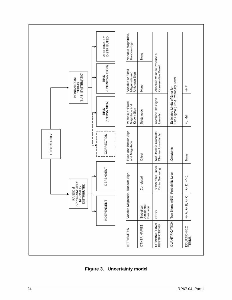
Figure 3. Uncertainty model

24 RP67.04, Part II

While the basic uncertainty formula can be used for any instrumentation application, care shouldbe taken when applying the formula in applications containing nonlinear modules or functions.While the term can still be random and independent, its magnitude is a function of the input andthe transfer function of the module. This requires the calculation of uncertainty for instrumentchannels containing nonlinear modules to be performed for specific values of the input signal.

The most common of these in instrumentation and control systems is the square root extractor ina flow channel. For these channels, the uncertainty value changes with the value of flow and,therefore, should be determined for each specific flow of interest.

The basic uncertainty combination formula can be applied to the determination of either amodule uncertainty or a total instrument channel uncertainty. The results are independent of theorder of combination as long as the dependent terms and bias terms are accounted for properly.For example, the uncertainty of a module can be determined from its individual terms and thencombined with other module uncertainties to provide an instrument channel uncertainty, or all ofthe individual module terms can be combined in one instrument channel uncertainty formula. Theresult will be the same. The specific groupings and breakdown of an uncertainty formula can bevaried for convenience of understanding.

6.2 Uncertainty data

The basic model used in this methodology requires that the user categorize instrumentuncertainties as random, bias, or random abnormally distributed bias. Guidelines for combiningthese categories of uncertainties to determine the module of overall instrument channeluncertainty are provided in 6.3. It is the purpose of this section to provide an understanding ofcategories of instrument uncertainty and some insight into the process of categorizinginstrumentation based on performance specifications, test reports, and the utility's owncalibration data.

The determination of uncertainty estimates is an iterative process that requires the developmentof assumptions and, where possible, verification of assumptions based on actual data. Ultimately,the user is responsible for defending the assumptions that affect the basis of the uncertaintyestimates.

It should not be assumed that, since this methodology addresses three categories of uncertainty,all three should be used in each uncertainty determination. Additionally, it should not be assumedthat instrument characteristics should fit neatly into a single category. Data may require, forexample, that an instrument's static pressure effect be represented as a random uncertainty withan associated bias.

6.2.1 Categories of uncertainty

6.2.1.1 Random uncertainties

In ANSI/ISA-S51.1-1979, random uncertainties are referred to as a quantitative statement of thereliability of a single measurement or of a parameter, such as the arithmetic mean value,determined from a number of random trial measurements. This is often called the statisticaluncertainty and is one of the so-called precision indices. The most commonly used indices,usually in reference to the reliability of the mean, are the standard deviation, the standard error(also called the standard deviation of the mean), and the probable error.

It is usually expected that those instrument uncertainties that a manufacturer specifies as havinga + magnitude are random uncertainties. However, the uncertainty must be zero-centered andapproximately normally distributed to be considered random. The hazards of assuming that the +in vendor data implies that the instrument's performance represents a normal statistical

RP67.04, Part II 25

distribution are addressed in 6.2.12. After uncertainties have been categorized as random, anydependencies between the random uncertainties should be identified.

6.2.1.1.1 Independent uncertainties

Independent uncertainties are those uncertainties for which no common root cause exists. It isgenerally accepted that most instrument channel uncertainties are independent of each other.

6.2.1.1.2 Dependent uncertainties

Because of the complicated relationships that may exist between the instrument channels andvarious instrument uncertainties, a dependency may exist between some uncertainties. Themethodology presented here provides a conservative means for addressing these dependencies.If, in the user's evaluation, two or more uncertainties are believed to be dependent, then, underthis methodology, these uncertainties should be added algebraically to create a new, largerindependent uncertainty.

Dependent uncertainties are those for which the user knows or suspects that a common rootcause exists that influences two or more of the uncertainties with a known relationship.

6.2.1.2 Nonrandom uncertainties

6.2.1.2.1 Bias (known sign)

A bias is a systematic instrument uncertainty that is predictable for a given set of conditionsbecause of the existence of a known direction (positive or negative).

For example, the static pressure effect of differential pressure transmitters, which exhibits apredictable zero shift because of changes in static pressure, is considered a bias. Additionalexamples of bias include head effects, range offsets, reference leg heatup or flashing, andchanges in flow element differential pressure because of process temperature changes. A biaserror may have an uncertainty associated with the magnitude.

6.2.1.2.2 Abnormally distributed uncertainties

Some uncertainties are not normally distributed. Such uncertainties are not eligible for SRSScombinations and are categorized as abnormally distributed uncertainties. Such uncertaintiesmay be random (equally likely to be positive or negative with respect to some value) butextremely non-normal.

This type of uncertainty is treated as a bias against both the positive and negative components ofa module's uncertainty. Refer to Appendix J on the use of the central limit theorem. Because theyare equally likely to have a positive or a negative deviation, worst-case treatment should be used.

6.2.1.2.3 Bias (unknown sign)

Some bias effects may not have a known sign. Their unpredictable sign should be conservativelytreated by algebraically adding the bias in the worse direction.

6.2.1.2.4 Correction

Errors or offsets that are of a known direction and magnitude should be corrected for in thecalibration of the module and do not need to be included in the setpoint calculation. See also6.2.6.4.

6.2.2 Module temperature effects

Most instruments exhibit a change in output as the ambient temperature to which they areexposed varies during normal plant operation above or below the temperature at which they werelast calibrated. As this change or temperature effect is an uncertainty, it should be accounted for

26 RP67.04, Part II

in instrument uncertainty calculations. To estimate the magnitude of the effect, the operatingtemperature (OT) extremes above or below the calibration temperature (CT) should be defined.Many times these temperatures should be assumed, based on conservative insight of guidance,if documented operating experience or design-basis room temperature calculations are notavailable. For example, it would be conservative to assume the maximum OT coincident with theminimum CT to maximize the temperature shift.

Once the temperatures are defined, the temperature effect uncertainty (TE) for each module canbe calculated using the manufacturer's published temperature effect specification. Commonly,the temperature effect is stated in vendor literature in one of the following two ways (expression inparentheses is an example). In each expression the temperature component (i.e., per 100°F) is achange in temperature within the vendor's specified range.

Either

a) TE = +X% span per Y°F

(for example, +1.0% span per 100°F)

or

b) TE = +X1% span at minimum span per Y°F

(for example, +5.0% span at minimum span per 100°F)

and

TE = +X2Y% span at maximum span per Y°F

(for example, +1.0% span at maximum span per 100°F)

If the temperature effect cannot be approximated by a linear relationship with temperature, aconservative approach is to use the bounding value for a temperature shift less than Y°F. If therelationship is linear, then the uncertainty can be calculated as shown below. For the TE asexpressed in (a),

TE = +X% (delta T)/Y (Eq. 6.3)

where

delta T = OTmax - CT or delta T = CT - OTmin , whichever is greater.

For example, using Equation 6.3 and the example value of TE of (a) above, if OT varies from50°F to 120°F and CT = 70°F,

TE = +(1.0%) (120 - 70)/100

= +0.5% span

Note that in the example above, the maximum operating temperature that the module will see(120°F) is a conservative value.

For (b), the uncertainty is not only temperature-dependent but span-dependent as well. To findthe temperature effect for the span of interest, assuming the temperature effect is a linearfunction of span and temperature, it is necessary to interpolate using the following expression:

(Eq. 6.4)X X1–

X2 X1–------------------- Span Min Span–

Max Span Min Span–----------------------------------------------------------=

RP67.04, Part II 27

Solving Equation 6.4 for X,

(X2 – X1) + X1 (Eq. 6.5)

If, for example, the span is 55 psi for a transmitter with an adjustable span range of 10-100 psi,the uncertainty in (b) for the same temperature conditions assumed in the previous example canbe calculated using Equation 6.5 and then Equation 6.3 as follows. In this case, however, X1 andX2 should be converted to process units so that units are the same.

X1 = (+5.0% span per 100°F)(10 psi/span)

= +0.5 psi per 100°F

X2 = (+1.0% span per 100°F)(100 psi/span)

= +1.0 psi per 100°F

X =

=

= +0.75 psi per 100°F

TE = (0.75)(120 - 70)/100

= +0.375 psi

Or in percent span

TE = +0.375 psi/55 psi x 100%

= +0.68% span.

This section dealt with module ambient temperature influence under normal conditions. Accidenteffects and ambient-induced process uncertainties (such as reference leg heatup) are discussedin 6.2.4 and Appendix B. If the particular instrument exhibits uncertainties under varying processtemperatures, a range of expected process temperatures needs to be included as an assumptionand the actual uncertainty calculated.

6.2.3 Module pressure effects

Some devices exhibit a change in output because of changes in process or ambient pressure. Atypical static pressure effect expression applicable to a differential pressure transmitter, wherethe listed pressure specification is the change in process pressure, may look like

+0.5% span per 1000 psi within the vendor's specified range.

This effect can occur when an instrument measuring differential pressure (dP) is calibrated at lowstatic pressure conditions but operated at high static pressure conditions. The manufacturergives instructions for calibrating the instrument to read correctly at the normal expected operatingpressure, assuming calibration was performed at low static pressure. This normally involvesoffsetting the span and zero adjustments by a manufacturer-supplied correction factor at the low-pressure (calibration) conditions so that the instrument will output the desired signal at the high-pressure (operating) conditions. To calculate the static pressure effect uncertainty (SP), anoperating pressure (OP) for which the unit was calibrated to read correctly and a pressurevariation (PV) above or below the OP should be determined. Once these points are defined, anexpression similar to Equation 6.3 can be used to calculate the static pressure effect (assumingthe effect is linear). Normally, the manufacturer lists separate span and zero effects.

X Span Min Span–( )Max Span Min Span–----------------------------------------------------------=

55 10–( ) 1.0 0.5–( )100 10–( )

---------------------------------------------------- 0.5+

45( ) 0.5( )90

------------------------- 0.5+

28 RP67.04, Part II

A caution needs to be discussed here concerning proper use of this uncertainty in calculations.The effect shown above is random. However, additional bias effects may need to be included dueto the way the static pressure calibration correction is done. For example, some instruments readlow at high static pressure conditions. If they have not been corrected for static pressure effects,a negative bias would need to be included in the uncertainty calculation.

Another effect related to pressure extremes is the overpressure effect. This uncertainty is due tooverranging the pressure sensor.

Ambient pressure variations will cause gage pressure instruments to shift up or down scaledepending on whether the ambient pressure at the instrument location decreases or increaseswithout a related change in the measured (process) variable. This occurs if the reference side ofthe process instrument is open to ambient pressure and the process is a closed system or if theprocess is open to atmosphere in an area with a different ambient pressure. This effect is a bias.The magnitude and direction will depend upon the variations in atmospheric pressure at theinstrument location. This may be a concern for gage pressure instruments in enclosed areassuch as reactor containment or containment enclosures.

6.2.4 Environmental effects - accident

For accident conditions, additional uncertainties associated with the high temperature, pressure,humidity, and radiation environment, along with the seismic response, may be included in theinstrument uncertainty calculations, as required.

Qualification reports for safety-related instruments normally contain tables, graphs, or both, ofaccuracy before, during, and after radiation and steam/pressure environmental and seismictesting. Many times, manufacturers summarize the results of the qualification testing in theirproduct specification sheets. More detailed information is normally available in the equipmentqualification report.

Because of the limited sample size typically used in qualification testing, the conservativeapproach to assigning uncertainty limits is to use the worst-case uncertainties. Discussions withthe vendor may be helpful to gain insight into the behavior of the uncertainty (i.e., should it beconsidered random or a bias?).

Using data from the qualification report (or module-specific temperature compensation data) inplace of design performance specifications, it is often possible to justify the use of loweruncertainty values that may occur at reduced temperature or radiation dose levels. Typically,qualification tests are conducted at the upper extremes of simulated DBE environments so thatthe results apply to as many plants as possible, each with different requirements. Therefore, it isnot always practical or necessary to use the results at the bounding environmental extremeswhen the actual requirements are not as limiting. Some cautions are needed, however, topreclude possible misapplication of the data.

a) The highest uncertainties of all the units tested at the reduced temperature or dose should be used. This is to ensure that bounding uncertainties are used in the absence of a statistically valid sample size. When extrapolating test data to lower than tested environmental data, a margin may need to be applied. Again, discussions with the vendor may provide helpful insight for performing these extrapolations.

b) The units tested should have been tested under identical or equivalent conditions and test sequences.

c) If a reduced temperature is used, ensure that sufficient "soak time" existed prior to the readings at that temperature to ensure sufficient thermal equilibrium was reached within the instrument case. In other words, if a transmitter case takes one minute to reach thermal

RP67.04, Part II 29

equilibrium, ensure that the transmitter was held at the reduced temperature at least one minute prior to taking readings.

Finally, it is sometimes possible to delete or reduce accident uncertainties from calculationsbased on the timing of the actuation function. For example, accident effects would not have to beconsidered for a primary reactor trip on low reactor coolant pressure if the trip function is creditedfor the design-basis, large break loss-of-coolant accident (LOCA) only. This is true because thetrip signal occurs very rapidly during the large immediate pressure decrease. Therefore, the tripfunction can be accomplished long before the environment becomes harsh enough to begin toaffect equipment performance significantly or affect the analysis results. Care should be taken inusing this technique to verify that the most limiting conditions for all of the applicable safetyanalyses are used.

6.2.5 Process measurement effects (PM)

Another source of instrument channel uncertainty that is not directly caused by equipment isprocess measurement effects. These are uncertainties induced by the physical characteristics orproperties of the process that is being measured. The decisions related to classifying processmeasurement uncertainties as random or bias should follow the guidance presented in 6.2.1.

Several types of process uncertainties may be encountered in instrumentation design. A few ofthe most common process uncertainty terms are discussed in the appendices. The applicabilityof all possible process measurement effects should be considered when preparing uncertaintycalculations.

6.2.6 Calibration uncertainty (CE)

Calibration is performed to verify that equipment performs to its specifications and, to the extentpossible, to eliminate bias uncertainties associated with installation and service; for example,head effects and density compensations. Calibration uncertainty refers to the uncertaintiesintroduced into the instrument channel during the calibration process. This includes uncertaintiesintroduced by test equipment, procedures, and personnel.

This section deals only with calibration uncertainties and how they should be included in the totalinstrument channel uncertainty calculation. However, other effects, such as installation effects (ifthe instrument is removed from the field for calibration and then reinstalled), should be accountedfor. Also, this recommended practice assumes that the calibration of a module is performed atapproximately the same temperature, so that temperature effects between calibrations areminimized.

6.2.6.1 Measuring and test equipment (M&TE) uncertainty

Several effects should be considered in establishing the overall magnitude of the M&TEuncertainty. These include the reference accuracy of the M&TE, the uncertainty associated withthe calibration of the M&TE, and the readability of the M&TE by the technician. Frequently, astandard M&TE uncertainty (such as +0.5%) is assumed. This approach is acceptable providedcare is taken to ensure the M&TE is bounded by the standard number.

The reference accuracy (RA) of the M&TE is generally available from the M&TE vendor. Note thatthe RA may be different for different scales on the M&TE.

M&TE should be periodically calibrated to controlled standards to maintain their accuracies.Typically, the RA of these standards is such that there is an insignificant effect on the overallchannel uncertainty. However, if a standard does not meet the guidelines of IEEE Standard 498;i.e., 4 to 1 better than the M&TE, this effect may need to be evaluated. If the RA of the standard isincluded in the uncertainty calculation, it may be combined with the RA of the M&TE using theSRSS techniques to establish a single value for the uncertainty of that piece of M&TE.

30 RP67.04, Part II

For example,

MTE = (RAMTE2 + RASTD

2)1/2 (Eq. 6.6)

where

MTE = uncertainty of the M&TE

RAMTE = reference accuracy of the M&TE

RASTD = reference accuracy of the controlled standard

The technician performing an instrument calibration (or the periodic calibration of M&TE)introduces additional uncertainty into the instrument loop. This uncertainty is introduced fromreading the instruments used in the calibration process. If the piece of M&TE has an analogscale, in addition to the movement uncertainty, the specific use of the scale should be consideredto assess the uncertainty. If the calibration process is arranged such that the scale divisions arealways used and there is no parallax, it is reasonable to assume no technician uncertainty sincethe pointer can be easily aligned with the fixed markings. If the points to be read lie betweendivisions, it is reasonable to assign an uncertainty. This turns into a judgment call on the part ofthe preparer. For example, if the scale spacing is "wide," +20% of the difference betweendivisions could be assigned to the technician's uncertainty. Where the divisions are more closelyspaced, +50% of the difference may be a better choice.

As before, any uncertainty assigned because of uncertainties in reading during the calibrationprocess should be converted to the appropriate units and combined with the M&TE uncertainty toobtain a more correct representation of the calibration process uncertainty. SRSS techniquesmay be used.

For example,

MTE = (RAMTE2 + RD2)1/2 (Eq. 6.7)

where

RD = reading uncertainty

If the M&TE has an uncertainty due to the standard used in its calibration and has a readinguncertainty, the uncertainty of the M&TE would be

MTE = (RAMTE2 + RASTD

2 + RD2)1/2 (Eq. 6.8)

The same units used to calculate the overall M&TE uncertainty should be used to calculate theinstrument channel uncertainty. If the instrument channel uncertainty calculation uses units ofpercent span, the M&TE uncertainty should be converted to percent span of the instrumentchannel. For example, if a piece of M&TE has a reference accuracy of 0.025 percent of its span,if its span is 0 to 3,000 psi, and if it is used in an instrument channel with a span of 1,000 psi, theM&TE reference accuracy is

(3,000 psi)/(1,000 psi) x 0.025% = 0.075% span of the instrument channel.

The M&TE uncertainty for a module should include the uncertainty of both the input and theoutput test equipment. Typically, both the input and output calibration test equipment areconsidered independent. These individual uncertainties may be combined by the SRSS methodto establish the overall M&TE uncertainty.

RP67.04, Part II 31

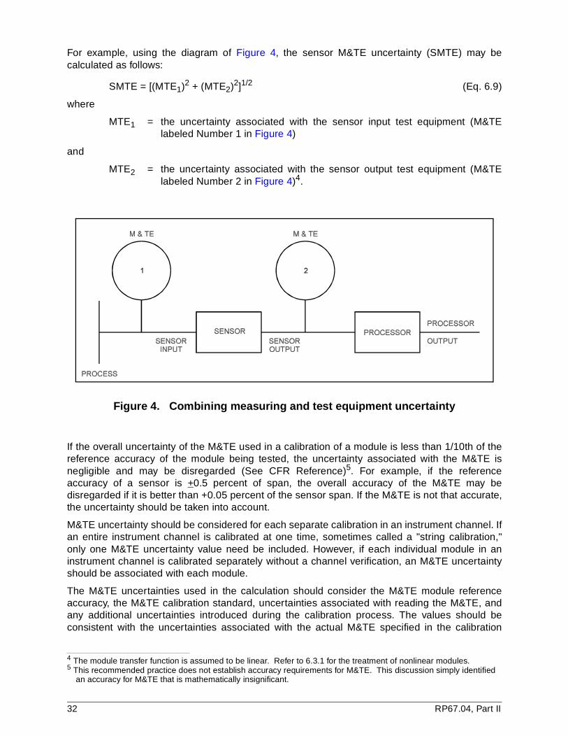
For example, using the diagram of Figure 4, the sensor M&TE uncertainty (SMTE) may becalculated as follows:

SMTE = [(MTE1)2 + (MTE2)2]1/2 (Eq. 6.9)

where

MTE1 = the uncertainty associated with the sensor input test equipment (M&TElabeled Number 1 in Figure 4)

and

MTE2 = the uncertainty associated with the sensor output test equipment (M&TElabeled Number 2 in Figure 4)4.

Figure 4. Combining measuring and test equipment uncertainty

If the overall uncertainty of the M&TE used in a calibration of a module is less than 1/10th of thereference accuracy of the module being tested, the uncertainty associated with the M&TE isnegligible and may be disregarded (See CFR Reference)5. For example, if the referenceaccuracy of a sensor is +0.5 percent of span, the overall accuracy of the M&TE may bedisregarded if it is better than +0.05 percent of the sensor span. If the M&TE is not that accurate,the uncertainty should be taken into account.

M&TE uncertainty should be considered for each separate calibration in an instrument channel. Ifan entire instrument channel is calibrated at one time, sometimes called a "string calibration,"only one M&TE uncertainty value need be included. However, if each individual module in aninstrument channel is calibrated separately without a channel verification, an M&TE uncertaintyshould be associated with each module.

The M&TE uncertainties used in the calculation should consider the M&TE module referenceaccuracy, the M&TE calibration standard, uncertainties associated with reading the M&TE, andany additional uncertainties introduced during the calibration process. The values should beconsistent with the uncertainties associated with the actual M&TE specified in the calibration

4 The module transfer function is assumed to be linear. Refer to 6.3.1 for the treatment of nonlinear modules.5 This recommended practice does not establish accuracy requirements for M&TE. This discussion simply identified

an accuracy for M&TE that is mathematically insignificant.

32 RP67.04, Part II

procedure. This is to allow the technicians performing instrument calibrations to remain within theassumptions of the setpoint uncertainty calculation. In practice, this may mean specifying in theprocedures and in the calculation the specific model of test equipment to be used and the scaleon which the test equipment is to be read. An alternative to this would be to establish a boundingreference accuracy for the M&TE in the calibration procedure and then establish a boundingassumption with appropriate justification for the M&TE uncertainty in the setpoint uncertaintycalculation.

6.2.6.2 Calibration tolerance

Calibration tolerance is the acceptable parameter variation limits above or below the desiredoutput for a given input standard associated with the calibration of the instrument channel.Typically, this is referred to as the setting tolerance of the width of the "as-left" band adjacent tothe desired response. To minimize equipment wear and to provide for human factorconsiderations, a band rather than a single value should be specified in the calibration procedure.This may be a symmetrical band about a setpoint; e.g., 109% +1%, or, in some cases, anonsymmetrical band about a setpoint; e.g., 110% +0%, -2%. This calibration tolerance is usuallybased on the reference accuracy of the module being calibrated. However, individual plantcalibration philosophies may specify a smaller or larger calibration tolerance. The size of thecalibration tolerance should be established based on the reference accuracy of the module, thelimitations of the technician in adjusting the module, and the need to minimize maintenance time.

Depending on the method of calibration or performance verification, an allowance for thecalibration tolerance may need to be included in the setpoint uncertainty calculation. If themethod of calibration or performance verification verifies all attributes of reference accuracy6,7

and the calibration tolerance is less than or equal to the reference accuracy, then the calibrationtolerance does not need to be included in the total instrument channel uncertainty. In this case,the calibration or performance verification has explicitly verified the instrument channelperformance to be within the allowance for the instrument channel's reference accuracy in thesetpoint uncertainty calculation. If the method of calibration or performance monitoring verifies allattributes of the reference accuracy and the calibration tolerance is larger than the referenceaccuracy, the larger value for the calibration tolerance may be substituted for the referenceaccuracy in the setpoint uncertainty calculation as opposed to inclusion of the calibrationtolerance as a separate term. For example, if the vendor's stated reference accuracy for aparticular module is 0.25%, but the calibration tolerance used in the procedure is 0.5%, the valueof 0.5% may be used for the reference accuracy of the module in the setpoint uncertaintycalculation with no additional allowance for calibration tolerance. In these cases, the calibrationtolerance is simply the term used to represent reference accuracy in the test's performance, andit does not represent a separate uncertainty term in the setpoint uncertainty calculation.

If the method of calibration or performance verification does not verify all attributes of thereference accuracy, the potential exists to introduce an offset in the instrument channel'sperformance characteristics that is not identified in the calibration or performance verification ofthe instrument channel. Usually, the offset is very small; however, the upper limit would be thecalibration tolerance. In this case, the reference accuracy and calibration tolerance are separateterms, and, therefore, both should be accounted for in the setpoint uncertainty calculation.Several methods are possible to account for the combination of reference and calibrationtolerance. The following discussion provides some examples of these methods but is notintended to be all-inclusive:

6 Reference accuracy is typically assumed to have four attributes: linearity, hysteresis, dead band, and repeatability. 7 ANSI/ISA-S51.1 indicates that an instrument channel should be exercised up and down a number of times to verify

reference accuracy.

RP67.04, Part II 33

a) One bounding method is to account for not verifying all attributes of reference accuracy by the calibration or performance verification by including allowances for both in the setpoint uncertainty calculation as explicit terms.

b) Another method is to establish a calibration tolerance that is less than the reference accuracy. If the difference between calibration tolerance and reference accuracy accounts for the uncertainty of the various attributes that are not verified during calibration or performance verification, only reference accuracy would be included in the setpoint uncertainty calculation.

c) A third method is to determine an allowance based on uncertainty algorithms or magnitudes that are known to be conservative. This may result in sufficient margin to provide a bounding allowance for reference accuracy and calibration tolerance without explicit terms for them in the setpoint uncertainty calculation. An example of this method would be to algebraically add the reference accuracy, drift, and M&TE uncertainties for a module rather than taking the SRSS (which assumes that these uncertainties are independent) of these uncertainties. However, the availability of this margin should be demonstrated prior to implicit reliance on this method.

d) A fourth method is to include a specific allowance in the setpoint uncertainty calculation for the attributes of reference accuracy that are not verified in the calibration or performance verification. For example, if the calibration or performance verification does not exercise an instrument channel more than once to demonstrate repeatability, it may be appropriate to include an allowance for repeatability in the setpoint uncertainty calculation. If a channel performs functions in both the increasing and decreasing directions and the calibration or performance verification does not check the accuracy in both directions, it may be appropriate to provide an allowance for hysteresis in the setpoint uncertainty calculation. If the calibration or performance verification does not check accuracy in the area of the trip functions, it may be appropriate to provide an allowance for linearity in the setpoint uncertainty calculation.

6.2.6.3 "As-found/as-left" calibration values

During calibration of a module, "as-found" and "as-left" data are typically obtained and recorded.If practicable, the "as-found" data should be taken without previously exercising the module,thereby providing a better indication of how the module would have performed if called upon bychanges in the process. The difference between the "as-found" data of the current calibration andthe "as-left" data from the previous calibration represents the net effects of several uncertainties,including the repeatability (reference accuracy) and drift of the module over the calibrationinterval. If the ambient temperature in the area of the module was not the same for the twocalibrations, part of the difference between the "as-found" and "as-left" data may be due totemperature effects. "As-found" and "as-left" data may be analyzed to estimate a value for drift forthe module, recognizing that variations in environmental conditions and other uncertainties maybe present at the time of the calibration and, if appropriate, accounted for when analyzing "as-found" and "as-left" data.

Nominal values and generic module performance data may be used for calculating moduleuncertainties to establish setpoints for initial plant operation. These nominal values may berefined after sufficient operating experiences and plant-specific data are available. Plant-specificdata is more representative of each module's performance within its unique installation andapplications characteristics and can be used to calculate smaller module drift uncertainties.Reducing module drift uncertainties allows one to revise setpoints to provide increased marginbetween the setpoint and expected process conditions during normal plant operating conditions.However, care should be taken to ensure that the use of plant-specific data is based on generallyaccepted statistical principles since limited sample sets may be unnecessarily conservative.

34 RP67.04, Part II

6.2.6.4 Calibration corrections

Frequently, calibration procedures include corrections to account for the difference in instrumentperformance or readings between calibration conditions and normal operating conditions, suchas static pressure and head pressure corrections. If these corrections have been made, thesetpoint uncertainty calculation does not need to include them (however, the uncertainty of thesecorrections should be included). The fact that these corrections are made during calibrationshould be identified in the setpoint uncertainty calculation.

6.2.7 Drift

An assumption for the time intervals between recalibration of each instrument should be includedin the setpoint uncertainty calculation. This time interval is used to calculate the drift uncertainty(DR) for the instrument using manufacturer's specifications such as:

+0.25% URL for a six-month period.

This example illustrates how uncertainties in (% URL) percent upper range limit can be convertedto percent span (% span). For example, assume a pressure transmitter with a URL of 1000 psigis calibrated to 0-500 psig. With an 18-month test interval, the drift uncertainty is calculated asfollows:

DR = [+(0.25%)(URL)/(span)] (18 months/6 months)

= (+0.25%)(1000 psig/500 psig)(3)

= +1.5% span

This assumes the drift term is a linear function of time. In the absence of other data, it isconsidered reasonable, and perhaps conservative, to make this assumption.

Other methods for extending drift data may be used. If one assumes that drift during each driftperiod is random and independent, the SRSS of the individual drift periods between calibrationsmay be used. In this case, it would be

DR = +[(0.25% URL)2 + (0.25% URL)2 + (0.25% URL)2]1/2

since there are three 6-month periods in the 18-month calibration interval; or

DR = +[(3)(0.25% URL)2]1/2

DR = +0.433% URL

Some vendor data has also suggested that the majority of an instrument's drift will occur in thefirst several months following a calibration, and that the instrument output will not drift significantlyafter the "settle in period." In this case, the 6-month value provided by the vendor may beacceptable for the 18-month calibration interval.

Whichever method is used, it should be listed as an assumption to the setpoint uncertaintycalculation, and some justification should be provided. The term (URL/span) is a dimensionlessquantity commonly referred to as the turndown factor (TDF). It can be multiplied by anuncertainty term in % URL to convert directly to % span. Note that drift may be stated in % URLor % span. It was given in % URL previously simply to illustrate the use of the TDF.

It should also be noted that the test interval is the time between calibrations, including anyallowed extensions, and is not necessarily equivalent to the time between refueling outages. Thisshould be considered in estimating the value to be used for drift.

RP67.04, Part II 35

6.2.8 Module power supply variations

Most electronic instruments exhibit a change in output because of variations in power supplyvoltage. A typical manufacturer's specifications may read

+0.01% span per volt variation.

To calculate the uncertainty associated with the power supply effect (PS), a normal operatingvoltage (OV), and voltage variation (VV) should be determined. Once these points are defined, ifthe effect is linear, an expression similar to Equation 6.3 can be used to calculate the uncertaintyassociated with the power supply effect. Typically, this uncertainty is very small in comparison toother instrument channel uncertainties.

6.2.9 Additional considerations for digital signal processing

In channels using digital processing equipment, uncertainties are introduced by hardware forconversions between analog and digital domains and by the algorithms for digital arithmeticoperations. Values for analog to digital (A/D) and digital to analog (D/A) conversion uncertaintiesmay be obtained from the module manufacturers or through testing. Sources of uncertainty mayinclude: precision of computation, rounding or truncation uncertainties, process variable changesduring the deadband between data acquisition sampling scans, and inaccuracies of algorithmsfor transcendental functions or empirical curve fitting. The nature of the uncertainties contributedby the software (that is, whether they are statistical or algebraic) should be identified by thesoftware designer. When the uncertainties are characterized and quantified, they can becombined with propagated uncertainties by the methods described in 6.3. Further discussion isprovided in Appendix H.

6.2.10 Insulation resistance effects

Under the conditions of high humidity and temperature associated with high energy line breaks(HELB), cables, splices, connectors, terminal blocks, and penetrations experience a reduction ininsulation resistance (IR). Reduction in IR causes an increase in leakage currents betweenconductors and from individual conductors to ground. Leakage currents are negligibly smallunder normal conditions. These currents are essentially calibrated out during instrument channelcalibrations. However, under the HELB event, the leakage currents may increase to a level thatcauses significant uncertainty in measurement. The effect is particularly a concern for sensitive,low signal level circuits such as current transmitters, RTDs, and thermocouples. For a moredetailed discussion on determining the IR effect, see Appendix D.

6.2.11 Sources of uncertainty data

The most reliable method of developing and substantiating uncertainty data is to performcontrolled tests on the devices that impose the conditions that have the potential to causeuncertainties in the device, or to analyze the performance data gained from operation andmaintenance of the equipment. This method has been widely applied to determine theuncertainties due to extreme temperature, pressure, and radiation levels. The allowances derivedfrom the test should consider the ability of the test to replicate the conditions and the accuracyand thoroughness of the test as discussed in 6.2.4.

A more common source of data is from the instrument supplier. Performance specificationsshould be provided by instrument or reactor vendors. Data should include reference accuracy,drift (stability), environmental effects, and reference conditions. Since performance specificationsoften describe a product line, any single instrument may perform significantly better than thegroup specification. Performance specifications may be obtained through the review of publishedinformation or through communication with the vendor. Test data may or may not be available tosupport the performance specifications since this data is generally applied to conditions under

36 RP67.04, Part II

which the device routinely operates. Therefore, the performance specifications may have beeninformally validated through the use and maintenance of the equipment.

If performance summary data is not available or if it does not satisfy the needs of the users, rawtest data may need to be reevaluated or created from additional testing.

Occasionally, the situation arises when the data necessary for a setpoint calculation is not readilyavailable; that is, test results or vendor literature do not exist. Several approaches may be takenin these cases. If possible, it is usually best to obtain a recommendation from the manufacturer orother utility/customer based on its experience with the instrumentation. Another approach mightinclude performing circuit analysis of electronic circuits and/or using data associated with aninstrument with similar principles of operation, made by another manufacturer. In some casesthere may be no prudent alternative but the common practice of using engineering judgment, inlieu of vendor literature or test data. The use of engineering judgment in these cases must betempered by the importance of the setpoint, which can be defined in a graded approach setpointprogram. With any of these approaches it is appropriate to apply some conservatism to theuncertainty values and to provide written justification for the values utilized.

6.2.12 Interpretation of uncertainty data

The proper interpretation of uncertainty information is necessary to ensure the validity of thesetpoint calculation. Historically, there have been many different methods of representingnumerical uncertainty. Almost all suffer from the ambiguity associated with shorthand notation.The symbol ±, for example, without further explanation, is often interpreted as the symmetricprobability interval associated with a random, normally distributed uncertainty. Further, theprobability level may be assumed to be 50% (probable error), 68.27% (one sigma), 95.45% (twosigma), or 99.73% (three sigma). Still others may assume that the ± symbol defines the limits oferror (reasonable bounds) of bias or non-normally distributed uncertainties. Discussions with thevendor may provide helpful insight for interpreting performance specifications or test results.

It is the user's responsibility to avoid improper use of the vendor performance data. If a vendor-published value of an uncertainty term (source) is believed to contain a significant biasuncertainty, then the + value should be treated as estimated limit of error. Simple field tests(repeated measurement) by the user can give an indication of the random component of thepublished value, if separation of components is desirable. If based on engineering judgment, theterm is believed to represent only random uncertainties (no significant bias uncertainties), thenthe + value may be treated as a value suitable for inclusion in the SRSS combination.

One source of performance data that requires careful interpretation is that obtained during harshenvironment testing. Often such tests are conducted only to demonstrate functional capability ofa particular instrument in a particular harsh environment. This usually requires only a smallsample size and invokes inappropriate rejection criteria for a probabilistic determination ofinstrument uncertainties. This type of data base typically results in limits of error (reasonablebounds) associated with bias or non-normally distributed uncertainties.

The sample size should be considered prior to adjusting the measured net effects for normalenvironmental uncertainties, reference accuracies, etc. The results of such tests describe severalmutually exclusive categories of uncertainty. For example, the results of a severe environmenttest contain uncertainty contributions from the instrument reference accuracy, M&TE uncertainty,calibration uncertainty, and others, in addition to the severe environment effects. A conservativepractice is to treat the measured net effects as only uncertainty contributions due to the harshenvironment.

Occasionally, select test data may appear inconsistent with the majority of the test data collected.In this situation it may be possible to justify the inconsistent data as outliers. Analytical

RP67.04, Part II 37

techniques for this purpose are discussed in ANSI N15.15, ANSI/ASME PTC 19.1, and ANSI/ASTM E 178. Additionally, Appendix J provides further discussion on statistical analysis.

6.3 Calculating total channel uncertainty

The calculation of an instrument channel uncertainty should be done in a clear, straightforwardprocess. The actual calculation can be done with a single-loop equation that contains all potentialuncertainty values or by a series of related term equations. Either way, a specific instrumentchannel calculation should be laid out to coincide with a channel's layout from processmeasurement to final output module or modules.

The actual technique and layout of the calculation is influenced by the type of instrument channelbeing analyzed. While many channels can be analyzed using the basic formulas defined in 6.1,channels that contain modules with transfer functions such as an amplifier, summer, square rootextractor, etc., require special consideration. This is due to the effect the transfer function canhave on the incoming signal and its associated uncertainty. The module's transfer function will acton both the true signal and its uncertainty to develop an output. Thus, the uncertainty within asignal may be increased or decreased by a module's transfer function, with respect to the truesignal.

A detailed look at the propagation of uncertainty through functional modules is provided in 6.3.1.Both the equations developed using the techniques of 6.3.1 and the basic equations of 6.1 mustbe used to analyze a channel's uncertainty. A discussion on the application of the basic statisticalequations for an instrument channel that does not contain modules with transfer functions isprovided in 6.3.2, while 6.3.3 provides a discussion on the application of the uncertaintypropagation equations.

6.3.1 Equations for the propagation of uncertainties through functional modules

If signal conditioning modules such as scalers, amplifiers, summers, square root extractors,multipliers, etc., are used in the instrument channel, the module's transfer function should beaccounted for in the instrument setpoint/uncertainty calculation. The uncertainty of a signalconditioning module's output can be determined when the uncertainty of the input signal and theuncertainty associated with the module, as well as the module's transfer function, are known.Using partial derivatives or perturbation techniques (refer to Appendix K for a detailed discussionof these techniques), equations have been developed to determine the output signaluncertainties for several common types of signal conditioning modules and are presented inTable 1. The equations are applicable to all signal conditioning modules of that type, regardlessof the manufacturer.

The attributes of uncertainties such as randomness or independence are discussed in detail in6.2.1. For simplicity, the equations presented in Table 1 are based on the assumption that theinput uncertainties consist of either all random or all biased uncertainties. The user must takecare in applying these equations to individual instrument channel uncertainty calculations toensure that the probability and confidence levels of the data and resulting uncertainty values aremaintained. In balancing the requirements of calculation conservatism, probabilities, andoperating margins, it may be beneficial to optimize the uncertainty determination by computersimulation techniques. The more general case of uncertainties with both random and biasedcomponents is addressed in Appendix K.

It is important to note that the method of calibration or testing may directly affect the use of theinformation presented in this section. If, for example, a group of the modules for a particularinstrument channel is always tested and calibrated together, it may be treated as a singlemodule. The uncertainties associated with the output of the group treated as a single module

38 RP67.04, Part II

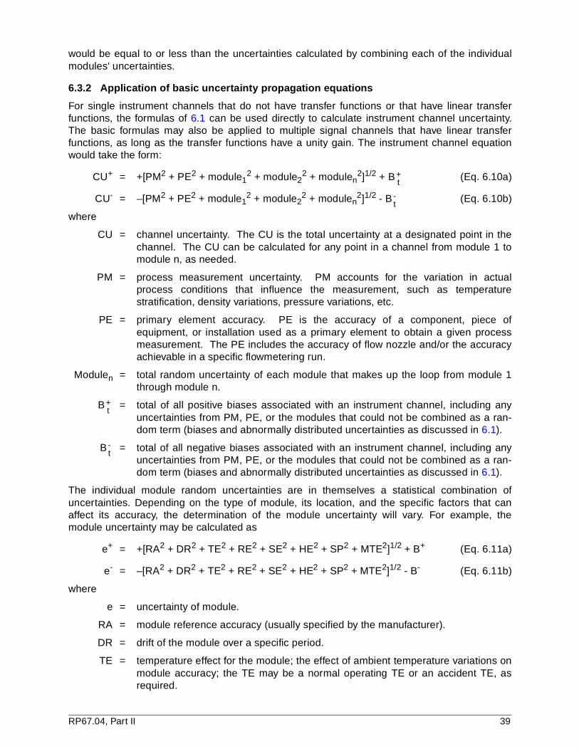
would be equal to or less than the uncertainties calculated by combining each of the individualmodules' uncertainties.

6.3.2 Application of basic uncertainty propagation equations

For single instrument channels that do not have transfer functions or that have linear transferfunctions, the formulas of 6.1 can be used directly to calculate instrument channel uncertainty.The basic formulas may also be applied to multiple signal channels that have linear transferfunctions, as long as the transfer functions have a unity gain. The instrument channel equationwould take the form:

CU+ = +[PM2 + PE2 + module12 + module2

2 + modulen2]1/2 + B (Eq. 6.10a)

CU- = –[PM2 + PE2 + module12 + module2

2 + modulen2]1/2 - B (Eq. 6.10b)

where

CU = channel uncertainty. The CU is the total uncertainty at a designated point in thechannel. The CU can be calculated for any point in a channel from module 1 tomodule n, as needed.

PM = process measurement uncertainty. PM accounts for the variation in actualprocess conditions that influence the measurement, such as temperaturestratification, density variations, pressure variations, etc.

PE = primary element accuracy. PE is the accuracy of a component, piece ofequipment, or installation used as a primary element to obtain a given processmeasurement. The PE includes the accuracy of flow nozzle and/or the accuracyachievable in a specific flowmetering run.

Modulen = total random uncertainty of each module that makes up the loop from module 1through module n.

B = total of all positive biases associated with an instrument channel, including anyuncertainties from PM, PE, or the modules that could not be combined as a ran-dom term (biases and abnormally distributed uncertainties as discussed in 6.1).

B = total of all negative biases associated with an instrument channel, including anyuncertainties from PM, PE, or the modules that could not be combined as a ran-dom term (biases and abnormally distributed uncertainties as discussed in 6.1).

The individual module random uncertainties are in themselves a statistical combination ofuncertainties. Depending on the type of module, its location, and the specific factors that canaffect its accuracy, the determination of the module uncertainty will vary. For example, themodule uncertainty may be calculated as

e+ = +[RA2 + DR2 + TE2 + RE2 + SE2 + HE2 + SP2 + MTE2]1/2 + B+ (Eq. 6.11a)

e- = –[RA2 + DR2 + TE2 + RE2 + SE2 + HE2 + SP2 + MTE2]1/2 - B- (Eq. 6.11b)

where

e = uncertainty of module.

RA = module reference accuracy (usually specified by the manufacturer).

DR = drift of the module over a specific period.

TE = temperature effect for the module; the effect of ambient temperature variations onmodule accuracy; the TE may be a normal operating TE or an accident TE, asrequired.

+t

-t

+t

-t

RP67.04, Part II 39

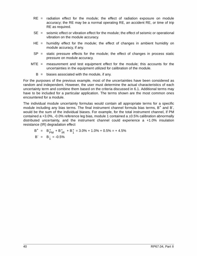
RE = radiation effect for the module; the effect of radiation exposure on moduleaccuracy; the RE may be a normal operating RE, an accident RE, or time of tripRE as required.

SE = seismic effect or vibration effect for the module; the effect of seismic or operationalvibration on the module accuracy.

HE = humidity effect for the module; the effect of changes in ambient humidity onmodule accuracy, if any.

SP = static pressure effects for the module; the effect of changes in process staticpressure on module accuracy.

MTE = measurement and test equipment effect for the module; this accounts for theuncertainties in the equipment utilized for calibration of the module.

B = biases associated with the module, if any.

For the purposes of the previous example, most of the uncertainties have been considered asrandom and independent. However, the user must determine the actual characteristics of eachuncertainty term and combine them based on the criteria discussed in 6.1. Additional terms mayhave to be included for a particular application. The terms shown are the most common onesencountered for a module.

The individual module uncertainty formulas would contain all appropriate terms for a specificmodule including any bias terms. The final instrument channel formula bias terms, B+ and B-,would be the sum of the individual biases. For example, for the total instrument channel, if PMcontained a +3.0%, -0.0% reference leg bias, module 1 contained a +0.5% calibration abnormallydistributed uncertainty, and the instrument channel could experience a +1.0% insulationresistance (IR) degradation effect

B+ = B + B + B = 3.0% + 1.0% + 0.5% = + 4.5%

B- = B = -0.5%

+PM

+IR

+1

-1

40 RP67.04, Part II

Table 1. Equations for propagation of input uncertainties through modules for various mathematical functions

FUNCTION/EQUATION (Notes 1, 2, 3, 4, and 7)

Fixed Gain Amp C = K * A

Summation C = (K1 * A) + (K2 * B)

Multiplication C = (K1 * A) * (K2 * B)

Division C = (K1 * A) / ( K2 * B)

eC(ALG) = K * eA(B) Eq. (6.12)

eC(SRSS) = K * eA(R) Eq. (6.13)

eC(ALG) = (K1 * eA(B)) + (K2 * eB(B)) Eq. (6.14)

eC(SRSS) = [ (K1 * eA(R))2 + (K * eB(R))

2 ]1/2 Eq. (6.15)

eC(ALG) = (K1 * K2) * [ (A * eB(B)) + (B * eA(B)) + (eA(B) * eB(B)) ]

≈ (K1 * K2) * [ (A * eB(B)) + (B * eA(B)) ]

Eq. (6.16)

eC(SRSS) = (K1 * K2) * [ (A * eB(R))2 + (B * eA(R))

2 + (eA(R) * eB(R))2 ]1/2

≈ (K1 * K2) * [ (A * eB(R))2 + (B * eA(R))

2 ]1/2Eq. (6.17)

Eq. (6.18)

Eq. (6.19)

eC(ALG)K1K2-------

B eA B( )*( ) A eB B( )*( )–

B2

--------------------------------------------------------------

* ≈

eC SRSS( )K1K2-------

B eA R( )*( )2A eB R( )*( )2

+[ ]1 2⁄

B2

----------------------------------------------------------------------------------

*≈

RP67.04, Part II 41

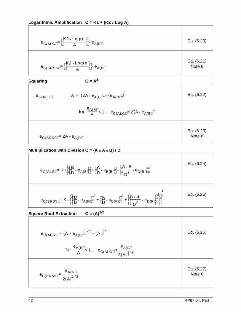
Logarithmic Amplification C = K1 + (K2 * Log A)

Squaring C = A 2

Multiplication with Division C = (K * A * B) / D

Square Root Extraction C = (A) 1/2

Eq. (6.20)

Eq. (6.21)Note 6

for ,

Eq. (6.22)

Eq. (6.23)Note 6

Eq. (6.24)

Eq. (6.25)

for ,

Eq. (6.26)

Eq. (6.27)Note 6

eC ALG( )K2 Log e( )*

A-------------------------------

eA B( )* ≈

eC SRSS( )K2 Log e( )*

A-------------------------------

eA R( )*≈

eC ALG( ) A 2A eA B( )*( ) eA B( )( )2+=

eA B( )A

-------------- 1< eC ALG( ) 2 A eA B( )*( )≈

eC SRSS( ) 2A eA R( )*≈

eC ALG( ) KBD---- eA B( )*

AD---- eB B( )*

A B*

D2

------------ eD B( )*

–+

*≈

eC SRSS( ) K BD---- eA R( )*

2 AD---- eB R( )*

2 A B*

D2

-------------- eD R( )* 2

+ +

12---

*≈

eC ALG( ) A eA B( )+( )1 2⁄A( )1 2⁄

–=

eA B( )A

-------------- 1< eC ALG( )eA B( )

2 A( )1 2⁄---------------------≈

eC SRSS( )eA R( )

2 A( )1 2⁄---------------------≈

42 RP67.04, Part II

Square Root with Multiplier C = K * (A * B)1/2

LEGEND

A, B, D = input signals (in signal units).

C = output signals (in signal units).

eA(R), eB(R), eD(R) = random-normal input uncertainties (in signal units).

eA(B), eB(B), eD(B) = biased input uncertainties (in signal units).

eC(ALG) = algebraic (biased) output uncertainty (in signal units).

eC(SRSS) = random-normal (or nearly normal) distributed output uncertainty (insignal units).

K, K1, K2 = arbitrary multipliers of input signals (dimensionless gains orattenuations).

NOTES:

1) The equations in this table describe the propagation of one or more input signal errorsthrough functional modules. Where multiple inputs are involved, the equation also accountsfor combination of the input errors. For the derivation of the equations for error propagationthrough multiple variable functions, see Section 6 of ANSI/ASME PTC 19.1.

2) Equations marked (ALG) must be used for bias errors or for errors with non-normaldistributions when the SRSS method would yield non-conservative results.

3) Equations marked (SRSS) may be used when input signal errors are random with anormal distribution. When input signal errors' distributions are not normal, these equationsshould not be used unless it can be demonstrated that results are conservative.

4) For single-input functions (e.g., Fixed Gain Amplifier), the "SRSS" designation means thata normal input error distribution results in normal (or near normal) output error that can becombined with other random-normal error terms using the SRSS method.

For multiple-input functions (e.g., Multiplier), the "SRSS" designation means that the outputerror is calculated using the SRSS method for combining the input errors that are random-normally distributed, and that output errors with this designation may be combined with othererror terms using the SRSS method.

5) Equation 6.13 is valid for input errors of any magnitude. The output distribution will be thesame as the input distribution because the transfer function is linear. The output error can becombined with other normally distributed error terms using the SRSS method.

Eq. (6.28)

Eq. (6.29)

eC ALG( )K2----

B eA B( )*( ) A eB B( )*( )+

A B*( )1 2⁄--------------------------------------------------------------*≈

eC SRSS( )K2----

B eA R( )*( )2A eB R( )*( )2

+[ ]1 2⁄

A B*( )1 2⁄----------------------------------------------------------------------------------*≈

RP67.04, Part II 43

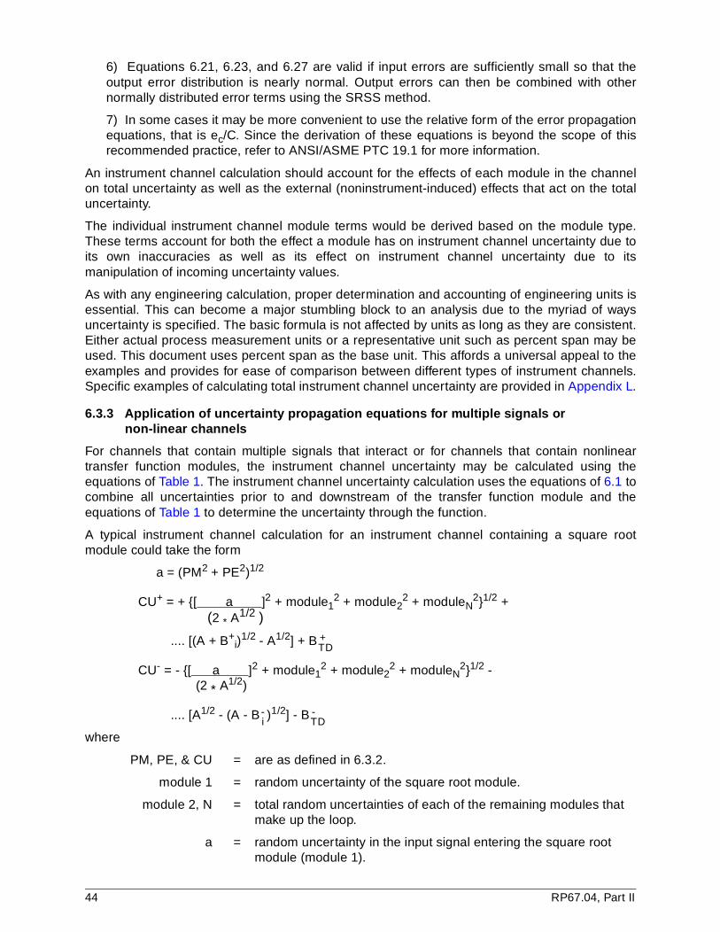
6) Equations 6.21, 6.23, and 6.27 are valid if input errors are sufficiently small so that theoutput error distribution is nearly normal. Output errors can then be combined with othernormally distributed error terms using the SRSS method.

7) In some cases it may be more convenient to use the relative form of the error propagationequations, that is ec/C. Since the derivation of these equations is beyond the scope of thisrecommended practice, refer to ANSI/ASME PTC 19.1 for more information.

An instrument channel calculation should account for the effects of each module in the channelon total uncertainty as well as the external (noninstrument-induced) effects that act on the totaluncertainty.

The individual instrument channel module terms would be derived based on the module type.These terms account for both the effect a module has on instrument channel uncertainty due toits own inaccuracies as well as its effect on instrument channel uncertainty due to itsmanipulation of incoming uncertainty values.

As with any engineering calculation, proper determination and accounting of engineering units isessential. This can become a major stumbling block to an analysis due to the myriad of waysuncertainty is specified. The basic formula is not affected by units as long as they are consistent.Either actual process measurement units or a representative unit such as percent span may beused. This document uses percent span as the base unit. This affords a universal appeal to theexamples and provides for ease of comparison between different types of instrument channels.Specific examples of calculating total instrument channel uncertainty are provided in Appendix L.

6.3.3 Application of uncertainty propagation equations for multiple signals or non-linear channels

For channels that contain multiple signals that interact or for channels that contain nonlineartransfer function modules, the instrument channel uncertainty may be calculated using theequations of Table 1. The instrument channel uncertainty calculation uses the equations of 6.1 tocombine all uncertainties prior to and downstream of the transfer function module and theequations of Table 1 to determine the uncertainty through the function.

A typical instrument channel calculation for an instrument channel containing a square rootmodule could take the form

a = (PM2 + PE2)1/2

CU+ = + {[ a ]2 + module12 + module2

2 + moduleN2}1/2 +

(2 * A1/2 )

.... [(A + B+i)

1/2 - A1/2] + B

CU- = - {[ a ]2 + module12 + module2

2 + moduleN2}1/2 -

(2 * A1/2)

.... [A1/2 - (A - B )1/2] - B

where

PM, PE, & CU = are as defined in 6.3.2.

module 1 = random uncertainty of the square root module.

module 2, N = total random uncertainties of each of the remaining modules thatmake up the loop.

a = random uncertainty in the input signal entering the square rootmodule (module 1).

+TD

-i

-TD

44 RP67.04, Part II

A = magnitude of the input signal to the square root module.

B , B = positive and negative biases associated with the input signal, if any.

B , B = total positive and negative biases associated with the modulesdownstream of square root module, if any.

In dealing with channels that contain nonlinear transfer functions, the uncertainty value isdependent on the relative magnitude of the input signal. This can be seen in the aboveequations. With the input uncertainty held constant, the instrument channel will increase as theinput signal decreases and vice versa. As a result, it is generally advantageous to calculate theuncertainty of loops containing nonlinear modules in terms of specific readings and not percentspan. The above square root extractor equation assumes an input magnitude of at least 50percent. For smaller values, a more rigid equation must be used to maintain the probability andconfidence levels of the data. Care must be taken in establishing the proper uncertainty transferfunction for nonlinear devices since the nonlinear devices can skew both the probability levelsand the confidence levels of the resulting uncertainty value.

One common method used in engineering calculations is to linearize a nonlinear function over arelatively small range of interest. Then errors can be propagated through the device usingrelatively simple linear techniques. When using this method, care must be taken to account forany modelling uncertainties generated by the linear approximation. One must also ensure thatthe uncertainty to be propagated is contained in the linearized range.

7 Establishment of setpoints

7.1 Setpoint relationships

The establishment of setpoints and the relationships between trip setpoint, allowable value,analytical limit, and safety limit are discussed in ISA-S67.04-1994. A thorough understanding ofthese terms is important in order to properly utilize the total instrument channel uncertainty in theestablishment of setpoints. Figure 5 presents the relative position of the safety limit, analyticallimit, allowable value, and the trip setpoint with respect to the normal operating point.

Safety limits are chosen to protect the integrity of physical barriers that guard against theuncontrolled release of radioactivity. The safety limits are typically provided in the plant technicalspecifications and safety analyses.

The analytical limit is established to ensure that the safety limit is not exceeded. The analyticallimit is developed from event analyses models that consider parameters such as process delays,rod insertion times, reactivity changes, instrument response times, etc. The development of theanalytical limit is outside the scope of this recommended practice; however, the use of theanalytical limit to obtain the allowable value and the trip setpoint will be discussed.

+i

-i

+TD

-TD

RP67.04, Part II 45

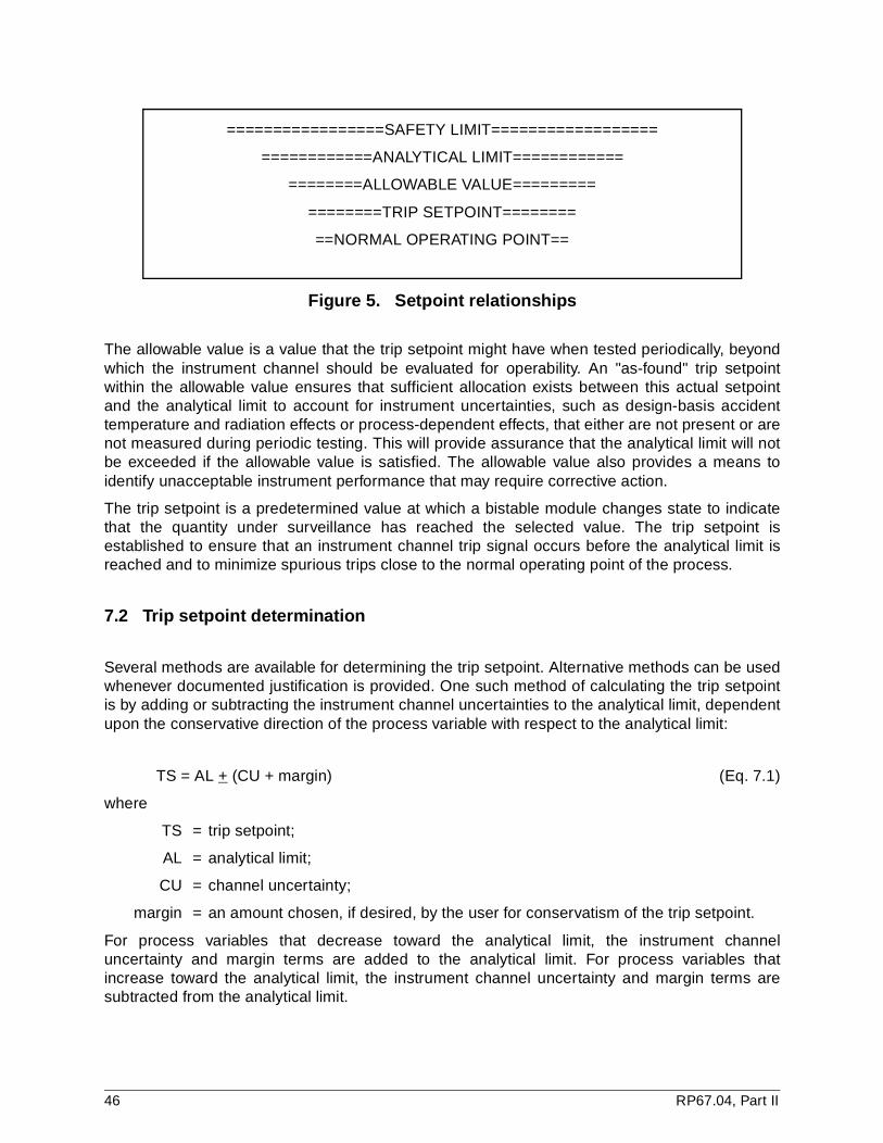
=================SAFETY LIMIT==================

============ANALYTICAL LIMIT============

========ALLOWABLE VALUE=========

========TRIP SETPOINT========

==NORMAL OPERATING POINT==

Figure 5. Setpoint relationships

The allowable value is a value that the trip setpoint might have when tested periodically, beyondwhich the instrument channel should be evaluated for operability. An "as-found" trip setpointwithin the allowable value ensures that sufficient allocation exists between this actual setpointand the analytical limit to account for instrument uncertainties, such as design-basis accidenttemperature and radiation effects or process-dependent effects, that either are not present or arenot measured during periodic testing. This will provide assurance that the analytical limit will notbe exceeded if the allowable value is satisfied. The allowable value also provides a means toidentify unacceptable instrument performance that may require corrective action.

The trip setpoint is a predetermined value at which a bistable module changes state to indicatethat the quantity under surveillance has reached the selected value. The trip setpoint isestablished to ensure that an instrument channel trip signal occurs before the analytical limit isreached and to minimize spurious trips close to the normal operating point of the process.

7.2 Trip setpoint determination

Several methods are available for determining the trip setpoint. Alternative methods can be usedwhenever documented justification is provided. One such method of calculating the trip setpointis by adding or subtracting the instrument channel uncertainties to the analytical limit, dependentupon the conservative direction of the process variable with respect to the analytical limit:

TS = AL + (CU + margin) (Eq. 7.1)

where

TS = trip setpoint;

AL = analytical limit;

CU = channel uncertainty;

margin = an amount chosen, if desired, by the user for conservatism of the trip setpoint.

For process variables that decrease toward the analytical limit, the instrument channeluncertainty and margin terms are added to the analytical limit. For process variables thatincrease toward the analytical limit, the instrument channel uncertainty and margin terms aresubtracted from the analytical limit.

46 RP67.04, Part II

EXAMPLE 1

The analytical limit used in a safety analysis for a high pressurizer pressure trip during a feedline break event is 2470 psia. Using the methods in Section 6, the instrument channeluncertainty for the instrument loop was determined to be as follows:

CU = +100 psi — the resulting uncertainty after combining all of the positive components;

and

-85 psi — the resulting uncertainty after combining all of the negative components.

Since the process is increasing toward the analytical limit, the resulting uncertainty aftercombining the negative components is used. With a margin of zero, then

TS = 2470 - (85 + 0) = 2385 psia.

The positive channel uncertainty of +100 psi is not used since the process is increasingtoward the analytical limit.

7.3 Allowable value

Several methods for determining the allowable value have been developed and are presently inuse. Three methods are illustrated in Figure 6. The allowance between the allowable value andthe trip setpoint should contain that portion of the instrument channel being tested for thesurveillance interval (monthly, quarterly, or refueling) and should account for no more than

a) drift (based on surveillance interval);

b) instrument calibration uncertainties for the portion of the instrument channel tested; and

c) instrument uncertainties during normal operation that are measured during testing (see Appendix I).

In Figure 6 and the discussion that follows, it is assumed that the process increases toward theanalytical limit. If the process decreases toward the analytical limit, the directions given would bereversed.

In the first and second methods shown in Figure 6, the allowable value (AV) is determined bycalculating the instrument channel uncertainty without including those items identified previouslyin 7.3 (drift, calibration uncertainties, and uncertainties observed during normal operations). Thisresult is then subtracted from the analytical limit (AL) to establish the AV. In the first method thetrip setpoint is then determined by subtracting from the AV the combination of the uncertainties:drift, calibration uncertainties, and uncertainties observed during normal operation. In thesecond method shown in Figure 6, the trip setpoint is calculated as described in 7.2.

RP67.04, Part II 47

Figure 6. Methods for determining the allowable value

The third method to calculate the AV illustrated in Figure 6 first calculates the trip setpoint asdescribed in 7.2. Then, an allowance for the three categories of instrument uncertainty (drift,calibration uncertainty, and uncertainties during normal operation) is calculated. This allowanceis then added to the trip setpoint to establish the AV. If the allowance is not determined in amethod that is consistent with the method used for the determination of the trip setpoint, a checkcalculation should be performed. For example, if an SRSS combination is used for determiningthe trip setpoint and an algebraic combination is used for the allowance between the trip setpointand the AV, a check calibration should be performed. The check calculation should provideassurance that the purpose of the AV is still satisfied by providing a large enough allowance toaccount for those uncertainties not measured during the test. If the check calculation identifiesthat there is not enough allowance between the AL and AV, the AV must be changed to providethe necessary allowance. In all cases the difference between the AV and the trip setpoint must beat least as large as the calibration tolerance discussed in 6.2.6.2, and, if it is not, the trip setpointmust be adjusted.

8 Other considerations

This section discusses selected subjects that may occasionally arise in instrument channelsetpoint/uncertainty calculations.

48 RP67.04, Part II

8.1 Correction for setpoints with a single side of interest

For many safety-related setpoints, interest is only in the probability that a single value of theprocess parameter is not exceeded, and the single value is approached only from one direction.In such situations, the uncertainty value associated with single-sided distributions is smaller thanthe value associated with double-sided distributions. The method to calculate these smalleruncertainties values is given below.

For normally distributed 95% probability uncertainties, standardized area distribution tables (seeM.R. Spiegel Reference), show that 95% of the population will have uncertainties between + 1.96 sigma, with 2.5% falling below -1.96 sigma and 2.5% falling above +1.96 sigma. If thereare increasing and decreasing trip limits, the appropriate limits to use are + 1.96 sigma.

For normally distributed uncertainties, the same tables show that 95% of the population will haveuncertainties less than +1.645 sigma (50% below the median and 45% between the median and+1.645 sigma) and that 95% of the population will have uncertainties greater than -1.645 sigma.If interest is only in the probability that a single value of the process parameter is not exceededand the single value is approached only from one direction, the appropriate limit to use for 95%probability is +1.645 sigma or -1.645 sigma as appropriate.

Using this technique, a positive uncertainty that has been calculated for a symmetrical case canbe reduced while maintaining 95% coverage of the population when a single parameter isapproached from only one direction. For example, if the original symmetric value was based on 2 sigma members, the reduction factor is 1.645/2.00 = 0.8225; if the original symmetric value wasbased on 1.96 sigma values, the reduction factor is 1.645/1.96 = 0.839.

EXAMPLE 2

CU+ = +2.00% span (2 sigma value)

The trip occurs at a single point when the process parameter is decreasing. Decreasing tripsare only delayed by positive errors, errors that could make the indicated trip parameter higherthan the actual trip parameter.

CU+ = 2.0 * 0.8225 = +1.645% span

CU- = not of concern

9 Interfaces

Setpoints for automatic actuation of safety equipment in nuclear power plants affect differentfunctional organizations and are affected by many plant activities. It is important that theseinterfaces be fully recognized in order to maintain the plant instrument settings in full support ofappropriate safety analysis and plant operational requirements. The following discussionidentifies organizations and activities that typically exist in commercial nuclear power plants.These are not intended to be all-inclusive but are representative of areas where communicationsare necessary between organizations responsible for some aspect of safety equipment setpointdetermination or control.

The safety analysis group is initially responsible for utilizing uncertainty allowances in theappropriate analysis, which would include the uncertainty of the analysis simulation. Typically, in

RP67.04, Part II 49

the past, few instrument characteristics were needed to generate analytic limits from safety limits.However, analytical methods are now taking into account the history and interrelationships ofequipment performance.

The thermohydraulic and neutronic models usually require a system response time limit that isaffected by both process and instrument response times. The determination for dynamic effectssuch as response-time limits is typically addressed in the accident analysis and is not includedwithin the scope of this recommended practice. If dynamic effects were not accounted for in thissafety analysis, additional uncertainty terms may be needed to account for them. Any designmodification that changes the instrument dynamic characteristics or relocates sensors (orsensing-line taps) should be evaluated for safety-analysis impact.

The group(s) responsible for the generation of the plant-technical specification limiting safetysystem settings decide on appropriate allowances for instrument safety channels. If hardwareallowances cannot be met by available vendors, iterations of the safety analysis or setpointdetermination may be necessary.

Any design modifications that affect the measurement process should be evaluated for effects onsetpoint determination. This can happen in a direct way, such as module replacement, or in amore subtle manner, such as through a support system (e.g., a modification to a room airconditioning unit/flow path). Proper module selection is important to match the ratings andperformance of the module to the instrument channel application and design requirements.Another activity that causes a reexamination of the safety analysis is the periodic fuel reload.During the reload process, a safety evaluation is performed to verify that the existing analysisremains applicable. If it is determined that the existing analyses are no longer valid, additionalsafety analyses are performed. At this point, the assumptions and results of the safety analysesshould be reviewed to determine their impact on the instrumentation setpoint determination.

The plant maintenance/instrumentation group is usually responsible for instrument calibrationand the collection of performance data. The authors of maintenance procedures should ensurethat appropriate limits are placed on the use of test equipment. This should include the M&TEitself, as well as any additional uncertainties covered by the calibration procedure or technique.

The setting tolerances specified in a maintenance procedure should also be checked forconsistency with the "as-left" tolerances in the setpoint determination calculation. Also, themethods of performance monitoring and the period between monitoring should agree with theassumptions in the setpoint calculations. In short, the operations and maintenance activities atthe plant should be consistent with the basis and assumptions in the uncertainty/setpointcalculation.

Trip setpoint values usually require transformation from process parameters to voltage or currentvalues. For example, an analog pressure transmitter loop may contain an electronic comparatorwhose trip setting is measured and set in milliamperes of current. This conversion or scalingprocess can typically be described as a simple linear equation that relates process variable unitsto measurement signal units. Thus, changes to trip setpoints may result in comparator settingchanges. Also, any changes to the linear transfer equation (such as the calibrated span, zerosuppression/elevation) may also result in a module setting change. In some cases, the scalingconversion may account for some effects that are variable during severe environment conditions.If so, care should be taken to account for the variance, preferably in the setpoint determinationcalculation. For example, a hydrostatic head may be considered constant in a scaling calculationbut may be subject to an elevated temperature during a design-basis accident. In this case, anadditional uncertainty term should describe changes from the normal operating condition.

In the continuing process of design allowance verification, personnel evaluating instrumentperformance should be cognizant of allowances used in the setpoint determination. Traditionally,the verification process has been directed toward module drift, which may include reference

50 RP67.04, Part II

accuracy, M&TE, temperature effects, etc. Observations of deteriorating performance shouldresult in equipment repair or replacement or a setpoint change. The latter action requiresinterfacing with the group responsible for the setpoint determination and documentation.

The plant operations group should participate in the review of setpoint determinations to ensurethat sufficient operational margins exist for operationally limiting setpoints. Inadequate marginsmay result in inadvertent (unnecessary) actuations of safety equipment during operationaltransients. Setpoint changes may also alter the accident sequence of events, which may requirereanalysis, emergency procedure changes, or retraining. For plants with simulator facilities, itmay be appropriate to install the setpoint change on the simulator to evaluate the effect on plantoperation before the setpoint is installed in the plant.

Any modification that results in a technical specification setpoint change is typically processedthrough a plant licensing group or the equivalent liaison with the USNRC. A close relationshipwith that group is important to determine if a nonsetpoint change to the technical specifications orsome other regulatory change affects the assumptions of a setpoint calculation. Similarrelationships may exist for the interface with other governmental agencies; for example, thoseconcerning environmental discharge limits.

There is also an interface with vendors. The interpretation of the results from vendor publicationsand reports should be consistent with the allowances of the appropriate setpoint determinationcalculation. Information concerning unexpected product performance should be discussed withvendor personnel in order to evaluate the impact on a plant's particular application. It isparticularly important that recommended maintenance practices be clearly and formallycommunicated to the product user.

10 Documentation

Uncertainty analysis and setpoint determination documentation for safety-related instrumentchannels forms a part of a facility's overall design-basis documentation. As such, the analysisand final determination should be included under the facility's nuclear quality assurance anddesign control programs.

The actual form of the uncertainty analysis may vary from plant to plant, but the level ofdocumentation required should not. Documented calculations for safety-related setpoints includethe following information:

a) Setpoint identification

b) Function

c) Analytical limit

d) Plant operating conditions under which setpoint is required

e) Design basis event conditions under which setpoint is required

f) Instrument channel or channels for which setpoint must be calculated

g) Portion of instrument channel required for setpoint

h) Identification of all uncertainty terms that affect setpoint determination

RP67.04, Part II 51

i) Assumptions used in conjunction with the uncertainty analysis

j) Method of uncertainty calculation

k) Trip setpoint and allowable value determination

l) References

The uncertainty analysis should use plant design documents as the source of input. The designinput should be included in the plant's design control process. Each source of design inputshould be clearly noted within the uncertainty analysis.

11 References

11.1 References used in text

AMERICAN NATIONAL STANDARDS INSTITUTE (ANSI)

ANSI N15.15-1974 Assessment of the Assumption of Normality (EmployingIndividual Observed Values).

ANSI Standard C39.4-1966, Specifications for Automatic Null-Balancing Electrical (Reaffirmed 1972) Measuring Instruments

ANSI Standard C85.1-1963 Terminology for Automatic Control.

Available from: American National Standards Institute11 West 42nd StreetNew York, NY 10036 Tel: (212) 642-4900

AMERICAN SOCIETY OF MECHANICAL ENGINEERS (ASME)

ASME MFC-3M-1989 Measurement of Fluid Flow in Pipes Using Orifices, Nozzles, and Venturi.

ANSI/ASME PTC 19.1-1985 Measurement Uncertainty, Part I.

Bean, H.S., Fluid Meters - Their Theory and Application Report of ASME ResearchCommittee on Fluid Meters, Sixth Edition, New York: American Society of MechanicalEngineers, 1971.

Available from: American Society of Mechanical Engineers345 East 47th StreetNew York, NY 10017 Tel: (212) 705-7722

AMERICAN SOCIETY FOR TESTING AND MATERIALS (ASTM)

ANSI/ASTM E 178-1980 Standard Practice for Dealing with Outlying Observations.

Available from: American Society for Testing and Materials1916 Race StreetPhiladelphia, PA 19103-1187 Tel: (215) 299-5585

52 RP67.04, Part II

INSTITUTE OF ELECTRICAL AND ELECTRONICS ENGINEERS (IEEE)

IEEE Standard 94-1991 Recommended Definitions of Terms for Automatic Generation Control on Electric Power Systems.

IEEE Standard 338-1987 Standard Criteria for the Periodic Testing of Nuclear Power Generating Station Safety Systems.

IEEE Standard 498-1990 Standard Requirements for the Calibration and Control of Measuring and Test Equipment Used in Nuclear Power Generating Stations.

IEEE Standard 603-1991 Standard Criteria for Safety Systems for Nuclear Power Generating Stations.

Available from: Institute of Electrical and Electronics Engineers 445 Hoes LaneP.O. Box 1331Piscataway, NJ 08855-1331 Tel: (800) 678-4333

ISA

ANSI/ISA-S37.1-1975 Electrical Transducer Nomenclature and Terminology.

ANSI/ISA-S51.1-1979 Process Instrumentation Terminology.

ISA-S67.04, Part I-1994 Setpoints for Nuclear Safety-Related Instrumentation.

Webb, R.C. and Beuchel, B.E., A Graded Approach to Setpoint Calculation Programs,Proceedings of the Thirty-fifth Power Instrumentation Symposium of the Instrument Societyof America, 1992.

Available from: ISA67 Alexander DriveP.O. Box 12277Research Triangle Park, NC 27709 Tel: (919) 990-9200

MISCELLANEOUS

Beggs, W.J., "Statistics for Nuclear Engineers and Scientists, Part 1: Basic StatisticalInference," DOE Research and Development Report No. WAPD-TM-1292, February, 1981.

Bowker, A.H. and Lieberman, G.J., Engineering Statistics, Englewood Cliffs, NJ: Prentice-Hall, 1972.

Bury, K.V., Statistical Models in Applied Science, New York: John Wiley & Sons, 1975.

Hammersley, J.M. and Handscomb, D.C., Monte Carlo Methods, London, Methuean, 1964.

Hauger, Edward B., Probabilistic Approaches to Design, New York: John Wiley & Sons, 1968.

Ku, H.H., Ed., Precision Measurement and Calibration, NBS SP300, Vol. I, Confidence andTolerance Intervals for the Normal Distribution by F. Proschan.

Ku, H.H., Ed., Precision Measurement and Calibration, NBS SP300, Vol. I, StatisticalConcepts in Metrology by H. H. Ku.

Meyer, P.L., Introductory Probability and Statistical Applications, New York: Addison-Wesley,1965.

Miller, R.W., Flow Measurement Engineering Handbook, New York: McGraw-Hill, 1983.

RP67.04, Part II 53

Spiegel, M.R., Theory and Problems of Probability and Statistics, Appendix C, Schaum'sOutline Series, New York: McGraw-Hill, 1975.

Zalkind, C.S. and Shinskey, F.G., The Application of Statistical Methods in Evaluating theAccuracy of Analog Instruments and Systems, Foxboro, MA: The Foxboro Company.

UNITED STATES CODE OF FEDERAL REGULATIONS

Title 10, Chapter I, Part 50, Paragraph 50.36 (c) (1)

Available from: Government Superintendent of DocumentsU.S. Printing OfficeWashington, D.C. 20402

UNITED STATES NUCLEAR REGULATORY COMMISSION

NUREG/CR-3691 An Assessment of Terminal Blocks in the Nuclear Power Industry, September 1, 1991.

Available from: U.S. Nuclear Regulatory CommissionOffice of Nuclear Reactor RegulationWashington, D.C. 20555

11.2 Informative references

AMERICAN SOCIETY FOR QUALITY CONTROL (ASQC)

ANSI/ASQC M1-1987 American National Standard for Calibration Systems.

Available from: American Society for Quality Control611 East Wisconsin AvenueMilwaukee, WI 53202-4606 Tel: (414) 272-8575

AMERICAN SOCIETY OF MECHANICAL ENGINEERS (ASME)

Interim Supplement 19.5 On Instruments and Apparatus, Application, Part II of Fluid Meters,ASME Research Committee on Fluid Meters, 1971.

ASME Steam Tables, 5th Edition, "Properties of Saturated and Superheated Steam."

Fink, Donald G., Standard Handbook for Electrical Engineers, New York: McGraw-Hill, 1976.

MISCELLANEOUS

Beers, Yardley, Introduction to the Theory of Errors, New York: Addison-Wesley, 1953.

Benedict, R.P., Fundamentals of Pressure, Temperature, and Flow Measurement, New York:John Wiley & Sons, 1967.

Doebelin, E.O., Measurement Systems, New York: McGraw-Hill, 1983.

Hahn, G.J. and Shapiro, S.S., Statistical Models in Engineering, New York: John Wiley &Sons, 1967.

Juran, J.M., Ed., Quality Control Handbook, New York: McGraw-Hill, 1962.

Liptak, Bela, and Venczel, Kriszta, Eds., Instrument Engineer's Handbook for ProcessMeasurement, Chapter 2.12, New York: Chilton Book Company, 1982.

54 RP67.04, Part II

Lode, T., et al., "Error Analysis with Applications to Platinum Resistance TemperatureSensors," Rosemount Bulletin 9628, Appendix K.

Middlemiss, Ross R., Differential and Integral Calculus, New York: McGraw-Hill, 1946.

ISA

SAMA PMC 20.1 (For informational purposes only)

Available from: ISA67 Alexander DriveP.O. Box 12277Research Triangle Park, NC 27709 Tel: (919) 990-9200

RP67.04, Part II 55

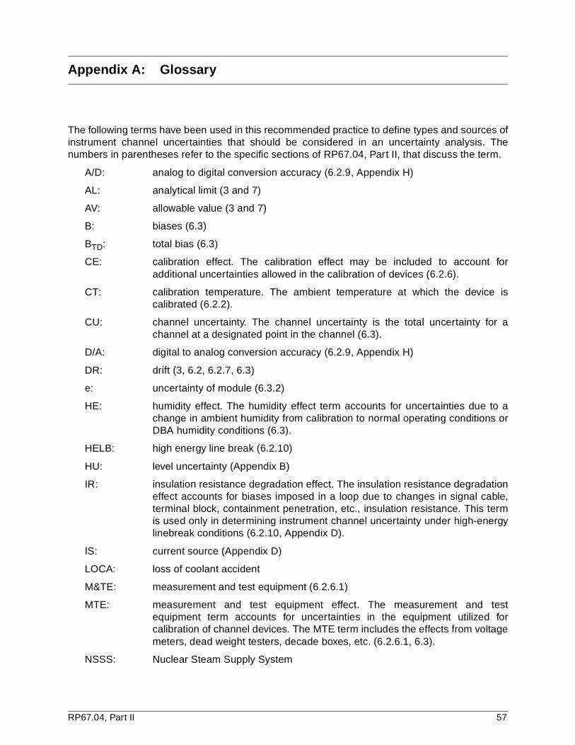
Appendix A: Glossary

The following terms have been used in this recommended practice to define types and sources ofinstrument channel uncertainties that should be considered in an uncertainty analysis. Thenumbers in parentheses refer to the specific sections of RP67.04, Part II, that discuss the term.

A/D: analog to digital conversion accuracy (6.2.9, Appendix H)

AL: analytical limit (3 and 7)

AV: allowable value (3 and 7)

B: biases (6.3)

BTD: total bias (6.3)

CE: calibration effect. The calibration effect may be included to account foradditional uncertainties allowed in the calibration of devices (6.2.6).

CT: calibration temperature. The ambient temperature at which the device iscalibrated (6.2.2).

CU: channel uncertainty. The channel uncertainty is the total uncertainty for achannel at a designated point in the channel (6.3).

D/A: digital to analog conversion accuracy (6.2.9, Appendix H)

DR: drift (3, 6.2, 6.2.7, 6.3)

e: uncertainty of module (6.3.2)

HE: humidity effect. The humidity effect term accounts for uncertainties due to achange in ambient humidity from calibration to normal operating conditions orDBA humidity conditions (6.3).

HELB: high energy line break (6.2.10)

HU: level uncertainty (Appendix B)

IR: insulation resistance degradation effect. The insulation resistance degradationeffect accounts for biases imposed in a loop due to changes in signal cable,terminal block, containment penetration, etc., insulation resistance. This termis used only in determining instrument channel uncertainty under high-energylinebreak conditions (6.2.10, Appendix D).

IS: current source (Appendix D)

LOCA: loss of coolant accident

M&TE: measurement and test equipment (6.2.6.1)

MTE: measurement and test equipment effect. The measurement and testequipment term accounts for uncertainties in the equipment utilized forcalibration of channel devices. The MTE term includes the effects from voltagemeters, dead weight testers, decade boxes, etc. (6.2.6.1, 6.3).

NSSS: Nuclear Steam Supply System

RP67.04, Part II 57

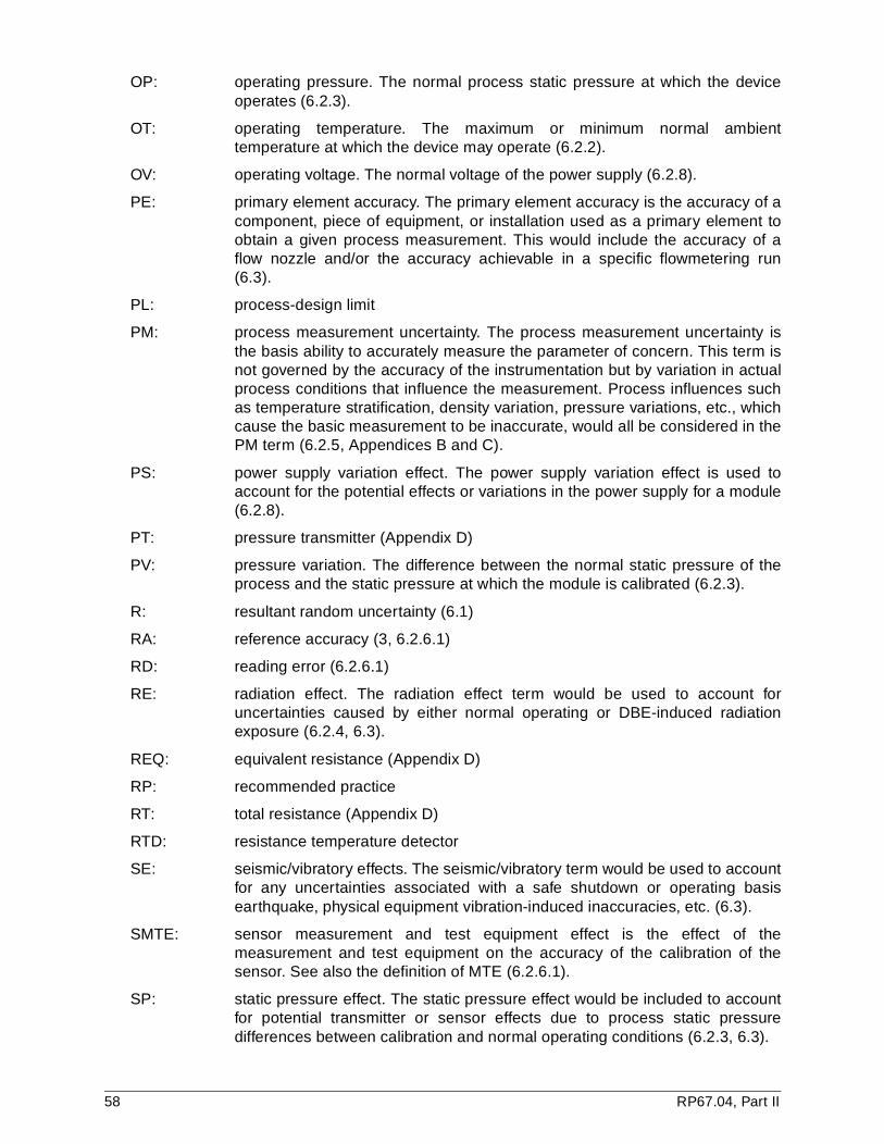
OP: operating pressure. The normal process static pressure at which the deviceoperates (6.2.3).

OT: operating temperature. The maximum or minimum normal ambienttemperature at which the device may operate (6.2.2).

OV: operating voltage. The normal voltage of the power supply (6.2.8).

PE: primary element accuracy. The primary element accuracy is the accuracy of acomponent, piece of equipment, or installation used as a primary element toobtain a given process measurement. This would include the accuracy of aflow nozzle and/or the accuracy achievable in a specific flowmetering run(6.3).

PL: process-design limit

PM: process measurement uncertainty. The process measurement uncertainty isthe basis ability to accurately measure the parameter of concern. This term isnot governed by the accuracy of the instrumentation but by variation in actualprocess conditions that influence the measurement. Process influences suchas temperature stratification, density variation, pressure variations, etc., whichcause the basic measurement to be inaccurate, would all be considered in thePM term (6.2.5, Appendices B and C).

PS: power supply variation effect. The power supply variation effect is used toaccount for the potential effects or variations in the power supply for a module(6.2.8).

PT: pressure transmitter (Appendix D)

PV: pressure variation. The difference between the normal static pressure of theprocess and the static pressure at which the module is calibrated (6.2.3).

R: resultant random uncertainty (6.1)

RA: reference accuracy (3, 6.2.6.1)

RD: reading error (6.2.6.1)

RE: radiation effect. The radiation effect term would be used to account foruncertainties caused by either normal operating or DBE-induced radiationexposure (6.2.4, 6.3).

REQ: equivalent resistance (Appendix D)

RP: recommended practice

RT: total resistance (Appendix D)

RTD: resistance temperature detector

SE: seismic/vibratory effects. The seismic/vibratory term would be used to accountfor any uncertainties associated with a safe shutdown or operating basisearthquake, physical equipment vibration-induced inaccuracies, etc. (6.3).

SMTE: sensor measurement and test equipment effect is the effect of themeasurement and test equipment on the accuracy of the calibration of thesensor. See also the definition of MTE (6.2.6.1).

SP: static pressure effect. The static pressure effect would be included to accountfor potential transmitter or sensor effects due to process static pressuredifferences between calibration and normal operating conditions (6.2.3, 6.3).

58 RP67.04, Part II

SRSS: square root of the sum of the squares (6.1, 6.2, Appendix J)

STD: reference accuracy of the controlled standard

TDF: turndown factor. The upper range limit divided by the calibrated span of thedevice (6.2.7).

TE: temperature effect. The ambient temperature effect term would be used toaccount for uncertainties due to the change in ambient temperature fromcalibration to normal operating conditions or DBA ambient temperature effects(6.2.2, 6.2.4, 6.3).

TS: trip setpoint (3 and 7)

URL: upper range limit. The maximum allowable span of the device (6.2.7).

VS: voltage source (Appendix D)

VV: voltage variation. The variation between normal voltage of the power supplyand the limits of voltages for the power supply (6.2.8).

RP67.04, Part II 59

Appendix B: Vessel/reference leg temperature effects on differentialpressure transmitters used for level measurement

When differential pressure transmitters are used to measure liquid level in vessels, changes indensity of the reference leg fluid, the vessel fluid, or both, it can cause uncertainties if the levelmeasurement system is not automatically compensated for density changes. This occursbecause differential pressure transmitters respond to hydrostatic (head) pressures, which aredirectly proportional to the height of the liquid column multiplied by the liquid density. Therefore,measurement uncertainty may be induced because, while the actual level in the vessel orreference leg remains constant, the liquid density changes as a function of pressure andtemperature. This changes the pressure delivered to the differential pressure transmitter, whichmakes the indicated level appear different from the actual level. The transmitter cannotdistinguish that the difference in pressure is caused by the density effect.

In level-measuring applications, two situations are frequently encountered. Although othersituations are common, it is not practical to cover the details of all of them. Instead, the situationsdescribed herein encompass the basic theory and methodology that can be applied to the othersituations. These are

a) Type A: The level measuring system is calibrated for assumed normal operating conditions. No automatic vessel or reference leg density compensation is provided; and

b) Type B: The level measuring system is automatically compensated for density variations of the fluid in the vessel, but no reference leg compensation is provided.

It is further assumed that the vessels are closed (non-vented) and contain a saturated mixture ofsteam and water; the reference leg is water-filled and saturated, and no temperature gradientexists along the length of the reference leg. Often the reference leg fluid is a compressed liquid,but, for the purpose of this discussion, it is assumed to be saturated. Use densities and specificvolumes as appropriate (e.g., subcooled, superheated). For simplicity, vessel growth is notconsidered in this example.

Before deriving the uncertainty equations for the situations described above, a review of levelmeasurement theory is presented. Figure B-1 shows a closed vessel containing a saturatedsteam/water mixture along with the explanations of the symbols used. From Figure B-1 thedifferential pressure supplied to the transmitter is obtained as follows:

dP = Pressure (HI) - Pressure (LO) (Eq. B.1)

Now,

Pressure (HI) = HR(SGR) + Static Pressure (Eq. B.2)

Pressure (LO) = HW(SGW) + HS(SGS) + Static Pressure (Eq. B.3)

Substituting Equations B.2 and B.3 into B.1,

dP = HR(SGR) - HW(SGW) - HS(SGS) (Eq. B.4)

Substituting (HR-HW) for HS in Equation B.4 yields

dP = HR(SGR) - HW(SGW) - (HR-HW)(SGS) (Eq. B.5)

RP67.04, Part II 61

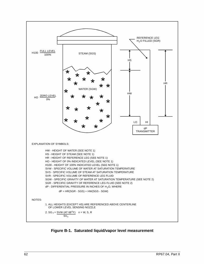
Figure B-1. Saturated liquid/vapor level measurement

STEAM (SGS)

REFERENCE LEGH O FILLED (SGR)2

FULL LEVEL

ZERO LEVEL

H100

EXPLANATION OF SYMBOLS:

NOTES:

SVn

n

o

HW - HEIGHT OF WATER (SEE NOTE 1)HS - HEIGHT OF STEAM (SEE NOTE 1)HR - HEIGHT OF REFERENCE LEG (SEE NOTE 1)HO - HEIGHT OF 0% INDICATED LEVEL (SEE NOTE 1)H100 - HEIGHT OF 100% INDICATED LEVEL (SEE NOTE 1)SVW - SPECIFIC VOLUME OF WATER AT SATURATION TEMPERATURESVS - SPECIFIC VOLUME OF STEAM AT SATURATION TEMPERATURESVR - SPECIFIC VOLUME OF REFERENCE LEG FLUIDSGW - SPECIFIC GRAVITY OF WATER AT SATURATION TEMPERATURE (SEE NOTE 2)SGR - SPECIFIC GRAVITY OF REFERENCE LEG FLUID (SEE NOTE 2)dP - DIFFERENTIAL PRESSURE IN INCHES OF H O, WHERE

1. ALL HEIGHTS (EXCEPT HS) ARE REFERENCED ABOVE CENTERLINEOF LOWER LEVEL SENSING NOZZLE

2. SG = SVW (AT 68 F) n = W, S, R

dP = HR(SGR - SGS) + HW(SGS - SGW)

2

HO

100%

0%

WATER (SGW)

dPTRANSMITTER

LO HI

HW

HS

HR

62 RP67.04, Part II

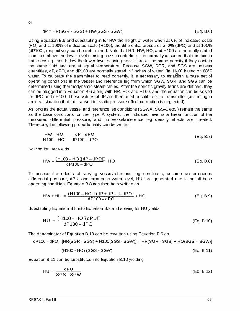
or

dP = HR(SGR - SGS) + HW(SGS - SGW) (Eq. B.6)

Using Equation B.6 and substituting in for HW the height of water when at 0% of indicated scale(HO) and at 100% of indicated scale (H100), the differential pressures at 0% (dPO) and at 100%(dP100), respectively, can be determined. Note that HR, HW, HO, and H100 are normally statedin inches above the lower level sensing nozzle centerline. It is normally assumed that the fluid inboth sensing lines below the lower level sensing nozzle are at the same density if they containthe same fluid and are at equal temperature. Because SGW, SGR, and SGS are unitlessquantities, dP, dPO, and dP100 are normally stated in "inches of water" (in. H2O) based on 68°Fwater. To calibrate the transmitter to read correctly, it is necessary to establish a base set ofoperating conditions in the vessel and reference leg from which SGW, SGR, and SGS can bedetermined using thermodynamic steam tables. After the specific gravity terms are defined, theycan be plugged into Equation B.6 along with HR, HO, and H100, and the equation can be solvedfor dPO and dP100. These values of dP are then used to calibrate the transmitter (assuming inan ideal situation that the transmitter static pressure effect correction is neglected).

As long as the actual vessel and reference leg conditions (SGWA, SGSA, etc.,) remain the sameas the base conditions for the Type A system, the indicated level is a linear function of themeasured differential pressure, and no vessel/reference leg density effects are created.Therefore, the following proportionality can be written:

(Eq. B.7)

Solving for HW yields

(Eq. B.8)

To assess the effects of varying vessel/reference leg conditions, assume an erroneousdifferential pressure, dPU, and erroneous water level, HU, are generated due to an off-baseoperating condition. Equation B.8 can then be rewritten as

(Eq. B.9)

Substituting Equation B.8 into Equation B.9 and solving for HU yields

(Eq. B.10)

The denominator of Equation B.10 can be rewritten using Equation B.6 as

dP100 - dPO= [HR(SGR - SGS) + H100(SGS - SGW)] - [HR(SGR - SGS) + HO(SGS - SGW)]

= (H100 - HO) (SGS - SGW) (Eq. B.11)

Equation B.11 can be substituted into Equation B.10 yielding

(Eq. B.12)

HW HO–H100 HO–------------------------------ dP dPO–

dP100 dPO–------------------------------------=

HW H100 HO–( ) dP dPO–( )dP100 dPO–

------------------------------------------------------------------= HO+

HW HU± H100 HO–( ) dP dPU±( ) dPO–{ }dP100 dPO–

------------------------------------------------------------------------------------------- HO+=

HU H100 HO–( ) dPU( )dP100 dPO–

----------------------------------------------------=

HU dPUSGS SGW–----------------------------------=

RP67.04, Part II 63

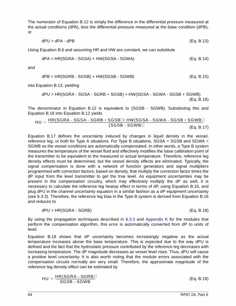
The numerator of Equation B.12 is simply the difference in the differential pressure measured atthe actual conditions (dPA), less the differential pressure measured at the base condition (dPB),or

dPU = dPA - dPB (Eq. B.13)

Using Equation B.6 and assuming HR and HW are constant, we can substitute

dPA = HR(SGRA - SGSA) + HW(SGSA - SGWA) (Eq. B.14)

and

dPB = HR(SGRB - SGSB) + HW(SGSB - SGWB) (Eq. B.15)

into Equation B.13, yielding

dPU = HR(SGRA - SGSA - SGRB + SGSB) + HW(SGSA - SGWA - SGSB + SGWB)(Eq. B.16)

The denominator in Equation B.12 is equivalent to (SGSB - SGWB). Substituting this andEquation B.16 into Equation B.12 yields

(Eq. B.17)

Equation B.17 defines the uncertainty induced by changes in liquid density in the vessel,reference leg, or both for Type A situations. For Type B situations, SGSA = SGSB and SGWA =SGWB as the vessel conditions are automatically compensated. In other words, a Type B systemmeasures the temperature of the vessel fluid and effectively modifies the base calibration point ofthe transmitter to be equivalent to the measured or actual temperature. Therefore, reference legdensity effects must be determined, but the vessel density effects are eliminated. Typically, thesignal compensation is done with a network of function generators and signal multipliersprogrammed with correction factors, based on density, that multiply the correction factor times thedP input from the level transmitter to get the true level. As equipment uncertainties may bepresent in the compensation circuitry, which may effectively multiply the dP as well, it isnecessary to calculate the reference leg heatup effect in terms of dP, using Equation B.16, andplug dPU in the channel uncertainty equation in a similar fashion as a dP equipment uncertainty(see 6.3.3). Therefore, the reference leg bias in the Type B system is derived from Equation B.16and reduces to

dPU = HR(SGRA - SGRB) (Eq. B.18)

By using the propagation techniques described in 6.3.3 and Appendix K for the modules thatperform the compensation algorithm, this error is automatically converted from dP to units oflevel.

Equation B.18 shows that dP uncertainty becomes increasingly negative as the actualtemperature increases above the base temperature. This is expected due to the way dPU isdefined and the fact that the hydrostatic pressure contributed by the reference leg decreases withincreasing temperature. The dP magnitude decreases as vessel level rises. Thus, dPU will causea positive level uncertainty. It is also worth noting that the module errors associated with thecompensation circuits normally are very small. Therefore, the approximate magnitude of thereference leg density effect can be estimated by

(Eq. B.19)

HU HR SGRA SGSA– SGRB– SGSB+( ) HW SGSA SGWA– SGSB– SGWB+( )+SGSB SGWB–( )

---------------------------------------------------------------------------------------------------------------------------------------------------------------------------------------------------------------------------=

HU HR SGRA SGRB–( )SGSB SGWB–

--------------------------------------------------------=

64 RP67.04, Part II

This equation was developed from Equation B.17 letting SGSA = SGSB and SGWA = SGWB.Although the Type B system eliminates the process density effects, one should be cautioned thatother uncertainties will be present in the density compensation modules, sensor, and signaltransmission portions of the system. The net effect is that the dP signal will be compensated forconditions not exactly equal to the actual process conditions. Therefore, the propagationtechniques discussed in 6.3.3 and Appendix K should be used to ensure conservativeuncertainty allowances.

As previously discussed, the Type B system compensation equipment effectively "adjusts" thebase calibration conditions to match the actual vessel conditions. Therefore, when usingEquation B.19 the level error, HU, is determined at the vessel condition of interest by plugging inthe specific gravity steam and specific gravity water values for that condition, not the basecondition for which the transmitter is calibrated.

If the high pressure (HI) side of the transmitter had been connected to the lower nozzle and thelow pressure (LO) side had been connected to the upper nozzle, it can be shown by similarderivation that Equations B.17 and B.19 still apply. Equation B.18 becomes

dPU = HR(SGRB - SGRA) (Eq. B.20)

Because the denominator term in Equations B.17 and B.19 decreases with increasingtemperature, it is evident that the effect increases with rising vessel temperature. Furthermore,examination of the numerator of Equation B.17 reveals that the effect is maximized when HW isequal to H100. Examination of Equation B.19 reveals that an increasing reference legtemperature above the base conditions results in an increasing positive effect, assuming vesselconditions remain constant.

The equations above calculate uncertainties in actual engineering units. If it is desired to work inpercent span, the quantities HU and dPU can be converted to percent span by dividing each by(H100 - HO) or (dP100 - dPO), respectively, and multiplying the results by 100 percent. Aspreviously discussed, the sign of dPU must be considered based on which way the high and lowpressure sides of the dP transmitter are connected to the vessel.

Assume, for example, that a Type A system configured as shown in Figure B-1 has the followingconditions:

a) HR = 150 inches

b) HO = 50 inches

c) H100 = 150 inches

d) HW = 100 inches

e) Base conditions: Vessel = 532°F (saturated water) Reference leg = 68°F (saturated water)

f) Actual conditions: Vessel = 500°F (saturated water) Reference leg = 300°F (saturated water)

It is desired to determine HU using Equation B.17.

RP67.04, Part II 65

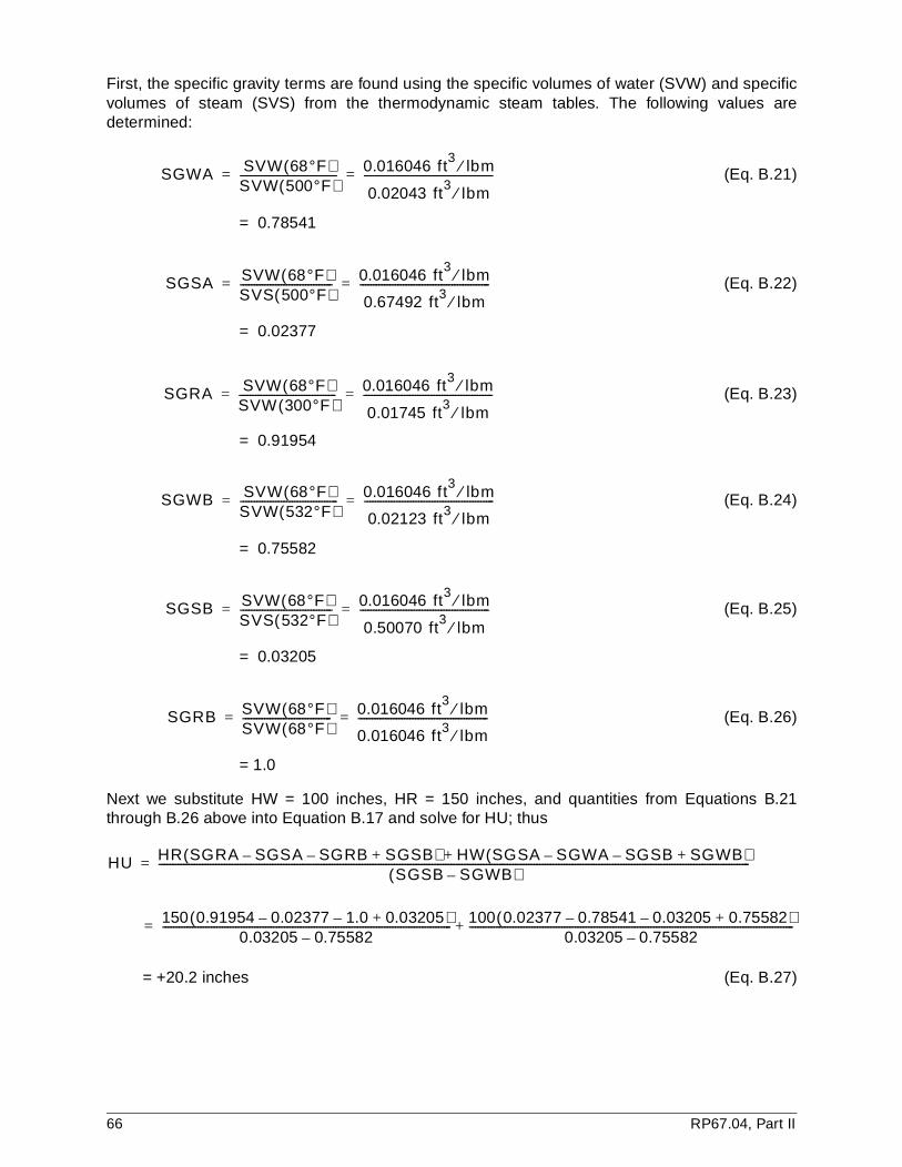
First, the specific gravity terms are found using the specific volumes of water (SVW) and specificvolumes of steam (SVS) from the thermodynamic steam tables. The following values aredetermined:

(Eq. B.21)

= 0.78541

(Eq. B.22)

= 0.02377

(Eq. B.23)

= 0.91954

(Eq. B.24)

= 0.75582

(Eq. B.25)

= 0.03205

(Eq. B.26)

= 1.0

Next we substitute HW = 100 inches, HR = 150 inches, and quantities from Equations B.21through B.26 above into Equation B.17 and solve for HU; thus

= +20.2 inches (Eq. B.27)

SGWA SVW 68°F( )SVW 500°F( )------------------------------------ 0.016046 ft

3lbm⁄

0.02043 ft3

lbm⁄------------------------------------------------= =

SGSA SVW 68°F( )SVS 500°F( )---------------------------------- 0.016046 ft

3lbm⁄

0.67492 ft3 lbm⁄------------------------------------------------= =

SGRA SVW 68°F( )SVW 300°F( )------------------------------------ 0.016046 ft3 lbm⁄

0.01745 ft3

lbm⁄------------------------------------------------= =

SGWB SVW 68°F( )SVW 532°F( )------------------------------------ 0.016046 ft

3lbm⁄

0.02123 ft3 lbm⁄------------------------------------------------= =

SGSB SVW 68°F( )SVS 532°F( )---------------------------------- 0.016046 ft3 lbm⁄

0.50070 ft3

lbm⁄------------------------------------------------= =

SGRB SVW 68°F( )SVW 68°F( )--------------------------------- 0.016046 ft

3lbm⁄

0.016046 ft3 lbm⁄------------------------------------------------= =

HU HR SGRA SGSA– SGRB– SGSB+( ) HW SGSA SGWA– SGSB– SGWB+( )+SGSB SGWB–( )

---------------------------------------------------------------------------------------------------------------------------------------------------------------------------------------------------------------------------=

150 0.91954 0.02377– 1.0– 0.03205+( )0.03205 0.75582–

----------------------------------------------------------------------------------------------------------- 100 0.02377 0.78541– 0.03205– 0.75582+( )0.03205 0.75582–

------------------------------------------------------------------------------------------------------------------------+=

66 RP67.04, Part II

In percent of indicated span,

= +20.2% span (Eq. B.28)

The preceding examples are typical for PWR steam generator level measurement. For BWRvessel level measurement, it is not uncommon for the reference and variable legs to traverseseveral temperature zones, and the assumption that the reference leg and variable leg see thesame temperature below the variable leg tap may not be valid. In these cases, the principlesdescribed in the examples are the same, but the equations become more complicated.

HU %( ) HUH100 HO–------------------------------ 100%×=

20.2150 50–---------------------- 100%×=

RP67.04, Part II 67

Appendix C: Effects on flow measurement accuracy

C.1 General flow measurement uncertainty

A detailed review of flow measurement is beyond the scope of this document; however, sometopics warrant discussion. ASME MFC-3M, plus H.S. Bean and R.W. Miller References addresshow to combine the different flow measurement uncertainties using the appropriate weighingfactors that indicate the impact of each uncertainty on the overall flow measurement uncertaintyequation. These uncertainties include density effects, bore tolerances, pipe diameters, thermalexpansion of the pipe and/or orifice, and coefficient uncertainty among other contributors. Forcalibrated installations, density changes may be the only significant source of uncertainty thatneeds to be addressed in addition to accuracy. Examples of accepted treatment of some of theseuncertainties follow.

C.2 Varying fluid density effects on flow orifice accuracy

In many nuclear plant applications, process liquid and gas flows are measured using orificeplates and differential pressure transmitters. The measurement of concern is either thevolumetric flow rate or the mass flow rate. Many reference books and standards have beenwritten using a wide variety of terminology to describe the mathematics of flow measurement, butin basic, simplified form the governing equations are

Q = K * (dP/Density)1/2 (Eq. C.1)

and

W = K * (dP * Density)1/2 (Eq. C.2)

where

Q = volumetric flow rate;

W = mass flow rate;

dP = differential pressure measured across the orifice;

Density = density of the fluid;

K = constant related to the beta ratio, units of measurement, and various correction factors.

As shown in Equations C.1 and C.2, the density of the fluid has a direct influence on the flow rate.Normally, a particular flow metering installation is calibrated or sized for an assumed normaloperating density condition. As long as the actual flowing conditions match the assumed density,related process errors should not be created. However, some systems, such as safety injection,perform dual roles in plant operation. During normal operation these systems can be aligned toinject makeup to the reactor coolant system from sources of relatively low-temperature water.During the recirculation phase of a LOCA, the pump suction is shifted to the containment sump,which contains water at much higher temperatures.

RP67.04, Part II 69

If the flow measuring system has been calibrated for the normal low-temperature condition,significant process uncertainties can be induced under accident conditions, when the highertemperature water (lower density) is flowing. Of course, the flow measurement could beautomatically compensated for density variations, but this is not the usual practice except onsystems such as feedwater, steam, or reactor coolant flow.

To examine the effects of changing fluid density conditions, a liquid flow process shall bediscussed. Examining Equation C.1, it is observed for all practical purposes that K is a constant.Actually, temperature affects K due to thermal expansion of the orifice, but this is assumed to beconstant for this discussion to quantify the effects of density alone. If the volumetric flow rate, Q,is held constant, it is seen that a decrease in density will cause a decrease in differential pressure(dP), which causes an uncertainty. This occurs because the differential pressure transmitter hasbeen calibrated for a particular differential pressure that corresponds to that flow rate. The lowerdP causes the transmitter to indicate a lower flow rate.

Assuming Q remains constant between a base condition (Density 1, that for which the instrumentis calibrated) and an actual condition (Density 2), an equality can be written between the baseflow rate (Q1) and actual flow rate (Q2) as shown below.

Q2 = Q1 (Eq. C.3)

or

K * (dP2/Density 2)1/2 = K * (dP1/Density 1)1/2 (Eq. C.4)

or

dP2/Density 2 = dP1/Density 1 (Eq. C.5)

(Eq. C.6)

Because density is the reciprocal of specific volume of fluid (SVF), Equation C.6 may be rewritten as

(Eq. C.7)

This equation shows that for an increasing temperature from condition 1 to condition 2, thedifferential pressure decreases. Therefore, the uncertainty, dPU, is equal to

dPU = dP2 - dP1 (Eq. C.8)

Rewriting dP2 from Equation C.7 as

dP2 = dP1 (SVF1/SVF2) (Eq. C.9)

and substituting in Equation C.8 yields

dPU = dP1 [(SVF1/SVF2) - 1] (Eq. C.10)

It is observed in Equation C.10, which is the equation for density effect on volumetric flow, thatthe absolute effect is maximized when dP1 is maximized. This occurs at the upper end of thecalibrated differential pressure span for which the transmitter is calibrated. This is also maximum

dP2

dP1---------- Density 2

Density 1---------------------------=

dP2

dP1---------- SVF

1

SVF2---------------=

70 RP67.04, Part II

calibrated flow. The effect varies from negative values for temperatures above the base value(SVF2 > SVF1) to zero for temperatures equal to the base value (SVF2 = SVF1) and finally topositive values for temperatures below the base value (SVF2 < SVF1). For mass flow, theequation can be derived in a similar fashion. Note that this method derives the differentialpressure error, which can be converted to a flow rate error using the flow versus differentialpressure relationship for the orifice.

As an example of the use of Equation C.10, assume an orifice plate is used to measure flow in awater system that is normally at 120°F. The orifice is sized to produce 100 inches of water at 100 gpm flow at 120°F. Assume further that under accident conditions the temperature rises to300°F at an actual flow of 50 gpm. It is desired to find dPU and the indicated flow.

The first step is to determine the relationship between Q and dP. Referring to Equation C.1 wereduce it to

Q = (Constant)(dP)1/2 (Eq. C.11)

assuming K and Density are constants for the particular situation. Plugging dP = 100 and Q = 100 into Equation C.11 yields

100 = (Constant)(100)1/2 (Eq. C.12)

or

(Eq. C.13)

Thus,

Q = 10(dP)1/2 (Eq. C.14)

Therefore, using Equation C.14 at the accident flow rate of 50 gpm, we can solve for dP1 asfollows:

Q = 10(dP1)1/2

50 = 10(dP1)1/2

or

(Eq. C.15)

Using thermodynamic steam tables, assuming saturation conditions,

SVF1 (at 120°F) = 0.016204 ft3/lbm (Eq. C.16)

SVF2 (at 300°F) = 0.01745 ft3/lbm (Eq. C.17)

Substituting Equations C.15, C.16, and C.17 into Equation C.10 yields

dPU = 25 [(0.016204/0.01745) - 1]

= -1.8 inches of water (Eq. C.18)

This can be converted to percent span, of course, by dividing dPU by the calibrated dP span andmultiplying the result by 100%.

Cons ttan 10010

---------- 10= =

dP1 50( )2

10( )2-------------- 25 inches of water= =

RP67.04, Part II 71

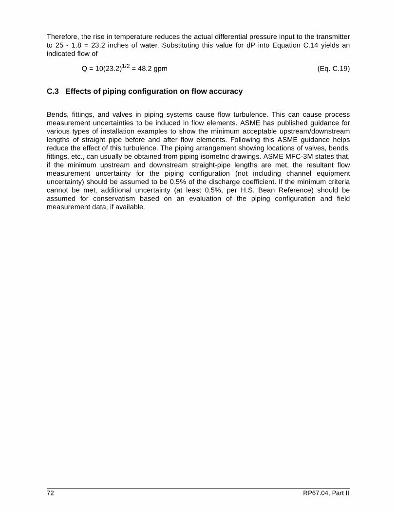
Therefore, the rise in temperature reduces the actual differential pressure input to the transmitterto 25 - 1.8 = 23.2 inches of water. Substituting this value for dP into Equation C.14 yields anindicated flow of

Q = 10(23.2)1/2 = 48.2 gpm (Eq. C.19)

C.3 Effects of piping configuration on flow accuracy

Bends, fittings, and valves in piping systems cause flow turbulence. This can cause processmeasurement uncertainties to be induced in flow elements. ASME has published guidance forvarious types of installation examples to show the minimum acceptable upstream/downstreamlengths of straight pipe before and after flow elements. Following this ASME guidance helpsreduce the effect of this turbulence. The piping arrangement showing locations of valves, bends,fittings, etc., can usually be obtained from piping isometric drawings. ASME MFC-3M states that,if the minimum upstream and downstream straight-pipe lengths are met, the resultant flowmeasurement uncertainty for the piping configuration (not including channel equipmentuncertainty) should be assumed to be 0.5% of the discharge coefficient. If the minimum criteriacannot be met, additional uncertainty (at least 0.5%, per H.S. Bean Reference) should beassumed for conservatism based on an evaluation of the piping configuration and fieldmeasurement data, if available.

72 RP67.04, Part II

Appendix D: Insulation resistance effects

D.1 Theory

Under conditions of high humidity and temperature associated with high energy line breaks(HELB), cables, splices, connectors, terminal blocks, and penetrations may experience areduction in insulation resistance (IR). The reduction in IR causes an increase in leakagecurrents between conductors and from individual conductors to ground. Leakage currents arenegligibly small under normal, nonaccident conditions. If channel calibrations are made, suchcurrents are essentially calibrated out. However, under HELB events the leakage currents mayincrease, causing an uncertainty in measurement. The effect can be a concern for circuits withsensitive, low level signals such as current transmitters, RTDs, thermocouples, etc. It isespecially of concern for channels with logarithmic signals (excore detectors, radiation monitors).For further details see NUREG/CR-3691.

The components of the instrument signal transmission system (cable, splices, connectors, etc.)are all constructed of insulating materials between electrical conductors. These insulatorsnormally are characterized by a low conductivity due to low concentration and low mobility ofions. However, under elevated temperature and humidity conditions, the ionic mobility increases,which leads to increased leakage current. The relationship between conductivity andtemperature for the insulator is given as

C = CO * e(-B/T) (Eq. D.1)

where

C = the ionic conductivity in ohms;

T = the temperature in degrees Kelvin (°K);

CO & B = constants.

It is observed in Equation D.1 that the conductivity increases exponentially with increasingtemperature. As insulation resistance is the reciprocal of conductivity, IR decreases withincreasing temperature. The rise in moisture also increases the surface conductivity effects,particularly with respect to exposed conductor surfaces such as in terminal blocks.

There also are instrument channels where lead wire resistance may be a contributor to the totalchannel uncertainty, such as thermocouples or RTD instrument channels. However, thisappendix addresses only IR effects.

D.2 Sources of IR data

Insulation resistance measurements are normally taken before, during, and after the LOCAsimulation phase of a qualification test. Normally, the IR data during the LOCA simulation is thedata of interest. Therefore, the IR data usually will be published within the qualification testreport. LOCA simulation tests may report cable IR based on IR or leakage current testsconducted on various cable types (e.g., shielded, unshielded, 2/c, 7/c, etc.) and measurementconfigurations (e.g., conductor-to-conductor, conductor-to-shield, multiple conductor-to-conductor/shield, etc.). The cable IR values extracted from the simulation tests for use in channel

RP67.04, Part II 73

uncertainty calculations should bound those expected for the particular channel's application. Ifnecessary, calculations can be performed, using the test configuration measured IR values, toobtain IR values for the channel cable configuration.

Usually the qualification test gives data for cable samples longer than 1 foot. This is becausepractical considerations normally require lengths longer than 1 foot for qualification testing due tothe size of the environmental chamber, mandrel size, etc. When calculating IR it is necessary todetermine an "ohms-foot" value for IR such that total resistance, RT, for actual installed cablelengths that vary in length can be easily calculated. As an example, assume a cable test sample25 feet in length exhibited a tested conductor-to-conductor resistance of 1.0 x 106 ohms. The 25-foot sample may be considered to be the lumped parallel resistance combination of 25 one-footsamples or

(Eq. D.2)

where R1 = R2 = ... R25, each resistance equal to the resistance (R) of a 1-foot sample. Thus,Equation D.2 becomes

1 = 25 RT R (Eq. D.3)

R = 25(RT) (Eq. D.4)

Thus, the individual 1-foot resistance is equal to R = 25 x (1.0 x 106) or 2.5 x 107 ohms - ft.

Typically, qualification tests use a bounding temperature profile so that the report will beapplicable to as many plants as possible, each with different peak accident temperatures. It isconservative but not always practical to use the IR values measured at the peak testedtemperature. It is acceptable to extrapolate or use actual tested IR values at lower temperaturesthat more closely bound or equal the user's peak temperature. However, as discussed earlier in6.2.4 and 6.2.11, caution must be applied when extrapolating test data.

D.3 IR effect example: Current source channel

A great majority of pressure, flow, level, etc., sensors used in the nuclear industry act essentiallylike ideal or constant current sources; that is, for a given process input, their output remains at aconstant current value, insensitive to loop resistance within a specified range. Figures D-1(a) andD-1(b) show a typical pressure transmitter (PT) and signal transmission system (blocks 1-5) to anindicator. The signal transmission components are in a harsh environment and, therefore, aresubject to IR degradation during an accident. The system is shielded up to component 2.However, the shield drain wire is included but not terminated to anything in the splice. The shieldis single-point grounded outside containment. The connector and penetration case are grounded.

An equivalent circuit schematic showing IR leakage paths and currents is shown in Figure D-1(c).Note that R11, R21, R31, etc., are the conductor-to-conductor IR values. Also, R12, R13, R22,R23, R32, R33, etc., are the conductor-to-shield values. The pressure transmitter is representedby current source, IS. The power supply is equivalent to voltage source, VS, and the indicator isequivalent to the load resistor, RL. Note that although the loop shown in Figure D-1(b) isungrounded, an air leakage path, RAIR, is shown to provide a return path for leakage currentsI12, I13, I22, I23, I32, I33, etc.

1RT-------- 1

RT-------- 1

R2-------- … 1

25------+ +=

74 RP67.04, Part II

Referring to Figure D-1(c) and D-1(d) the following equalities can be written:

(Eq. D.5)

(Eq. D.6)

(Eq. D.7)

These equations can be solved for REQ1, REQ2, and REQ3 and substituted into Figure D-1(d)for analysis. If we assume RAIR is several orders of magnitude larger than REQ2 and REQ3, thecircuit further simplifies to that shown in Figure D-1(e). This means

(Eq. D.8)

Thus Equation D.8 can be solved for RE. This leakage path gives rise to leakage current IE,which is also the error current. Under ideal conditions with no leakage due to IR degradation, thetransmitter current (IS) and load current (IL) would be equivalent. As shown in Figure D-1(e);however, IL and IS differ by the error current, IE.

Summing voltages in a clockwise fashion around the right-hand loop of the circuit, the followingequality can be written

VS = IE(REQ) + IL(RL) (Eq. D.9)

Solving for IE,

(Eq. D.10)

At node 1 of Figure D-1(c),

IL = IE + IS (Eq. D.11)

Substituting Equation D.11 into Equation D.10 yields

(Eq. D.12)

Rearranging Equation D.12,

IE(REQ) = VS - IE(RL) - IS(RL) (Eq. D.13)

IE(REQ + RL) = VS - IS(RL) (Eq. D.14)

(Eq. D.15)

1REQ1----------------- 1

R11----------- 1

R21----------- 1

R31----------- 1

R41----------- 1

R51-----------+ + + +=

1REQ2----------------- 1

R12----------- 1

R22----------- 1

R32----------- 1

R42----------- 1

R52-----------+ + + +=

1REQ3----------------- 1

R13----------- 1

R23----------- 1

R33----------- 1

R43----------- 1

R53-----------+ + + +=

1REQ------------- 1

REQ1----------------- 1

REQ2 REQ3+-----------------------------------------+=

IE VS IL RL( )–REQ

--------------------------------=

IE VS IE IS+( ) RL( )–REQ

--------------------------------------------------=

IE VS IS RL( )–REQ RL+

---------------------------------=

RP67.04, Part II 75

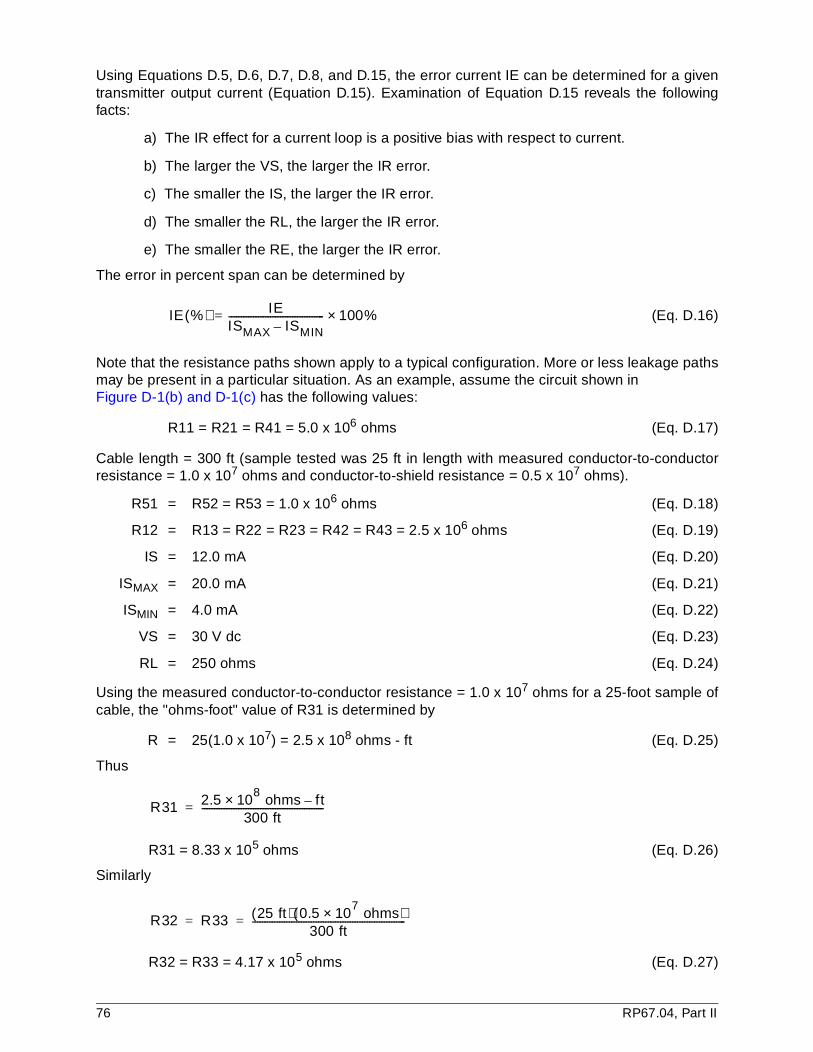
Using Equations D.5, D.6, D.7, D.8, and D.15, the error current IE can be determined for a giventransmitter output current (Equation D.15). Examination of Equation D.15 reveals the followingfacts:

a) The IR effect for a current loop is a positive bias with respect to current.

b) The larger the VS, the larger the IR error.

c) The smaller the IS, the larger the IR error.

d) The smaller the RL, the larger the IR error.

e) The smaller the RE, the larger the IR error.

The error in percent span can be determined by

(Eq. D.16)

Note that the resistance paths shown apply to a typical configuration. More or less leakage pathsmay be present in a particular situation. As an example, assume the circuit shown in Figure D-1(b) and D-1(c) has the following values:

R11 = R21 = R41 = 5.0 x 106 ohms (Eq. D.17)

Cable length = 300 ft (sample tested was 25 ft in length with measured conductor-to-conductorresistance = 1.0 x 107 ohms and conductor-to-shield resistance = 0.5 x 107 ohms).

R51 = R52 = R53 = 1.0 x 106 ohms (Eq. D.18)

R12 = R13 = R22 = R23 = R42 = R43 = 2.5 x 106 ohms (Eq. D.19)

IS = 12.0 mA (Eq. D.20)

ISMAX = 20.0 mA (Eq. D.21)

ISMIN = 4.0 mA (Eq. D.22)

VS = 30 V dc (Eq. D.23)

RL = 250 ohms (Eq. D.24)

Using the measured conductor-to-conductor resistance = 1.0 x 107 ohms for a 25-foot sample ofcable, the "ohms-foot" value of R31 is determined by

R = 25(1.0 x 107) = 2.5 x 108 ohms - ft (Eq. D.25)

Thus

R31 = 8.33 x 105 ohms (Eq. D.26)

Similarly

R32 = R33 = 4.17 x 105 ohms (Eq. D.27)

IE %( ) IEISMAX ISMIN–---------------------------------------= 100%×

R31 2.5 108× ohms ft–

300 ft--------------------------------------------------=

R32 R33 25 ft( ) 0.5 107 ohms×( )

300 ft---------------------------------------------------------------= =

76 RP67.04, Part II

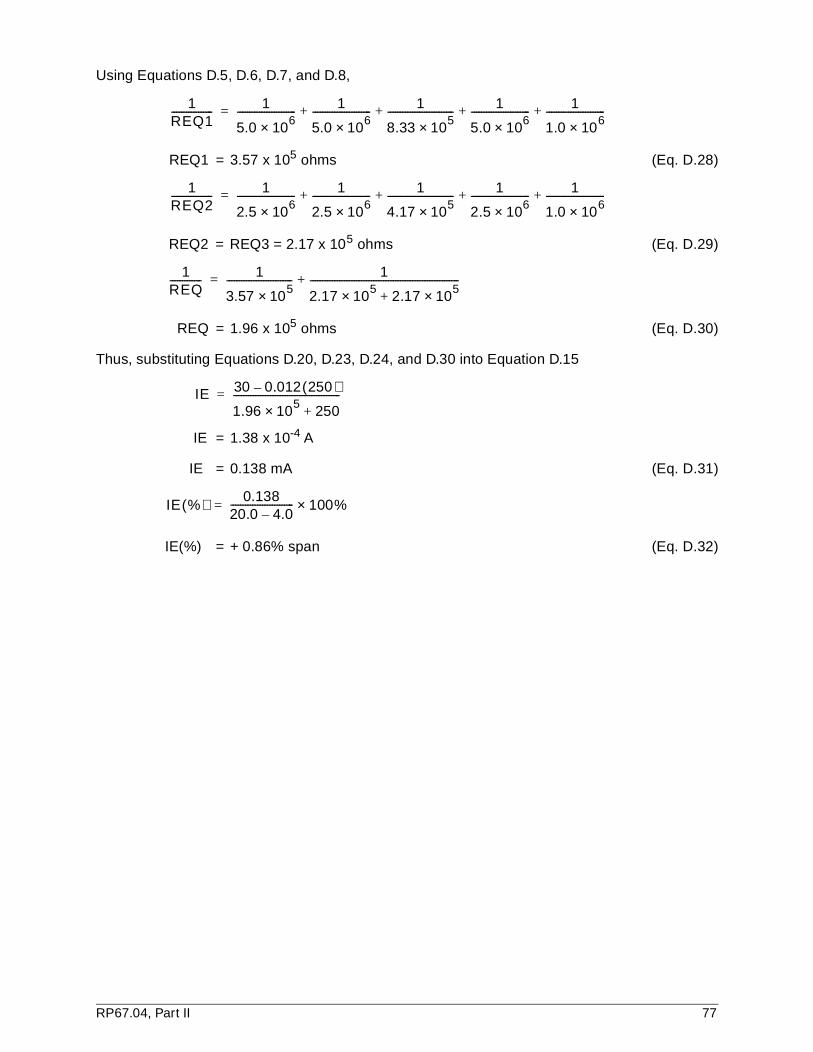
Using Equations D.5, D.6, D.7, and D.8,

REQ1 = 3.57 x 105 ohms (Eq. D.28)

REQ2 = REQ3 = 2.17 x 105 ohms (Eq. D.29)

REQ = 1.96 x 105 ohms (Eq. D.30)

Thus, substituting Equations D.20, D.23, D.24, and D.30 into Equation D.15

IE = 1.38 x 10-4 A

IE = 0.138 mA (Eq. D.31)

IE(%) = + 0.86% span (Eq. D.32)

1REQ1----------------- 1

5.0 106×------------------------ 1

5.0 106×------------------------ 1

8.33 105×--------------------------- 1

5.0 106×------------------------ 1

1.0 106×------------------------+ + + +=

1REQ2----------------- 1

2.5 106×------------------------ 1

2.5 106×------------------------ 1

4.17 105×--------------------------- 1

2.5 106×------------------------ 1

1.0 106×------------------------+ + + +=

1REQ------------- 1

3.57 105×--------------------------- 1

2.17 105× 2.17 105×+-------------------------------------------------------------+=

IE 30 0.012 250( )–

1.96 105× 250+--------------------------------------------=

IE %( ) 0.13820.0 4.0–-------------------------- 100%×=

RP67.04, Part II 77

Figure D-1. IR model for current loop

78 RP67.04, Part II

Figure D-1 (Cont'd). IR model for current loop

RP67.04, Part II 79

Figure D-1 (Cont'd). IR models for current loop

80 RP67.04, Part II

Appendix E: Plant specific as-found/as-left data

E.1 Overview

Instrument drift values for use in loop accuracy and setpoint calculations can be derived frommanufacturer's specifications or from plant-specific calibration history, if available. Guidelines fordetermining the manufacturer's specification for drift and combining values for larger timeintervals are provided in 6.2.7 of this recommended practice. This appendix provides guidelinesfor a data reduction methodology for plant specific as-found/as-left data to determine a value thatcan be used in this recommended practice. One approach is to substitute this value for the drift(DR) term in Equations 6.11a and 6.11b. Other approaches for the use of this value may beacceptable. The user is ultimately responsible for determining how to use the data.

It should be noted that the as-found/as-left data may include the combined effects of referenceaccuracy, inherent drift, measurement and test equipment, humidity, vibration, normal radiation,normal temperature, and power supply variations during the time period under surveillance.Additional terms may be included for a particular application as needed. A value for drift asobtained by this methodology is more conservative than the value of drift as defined in thisrecommended practice because it will include some or all of these other uncertainties.

E.2 Theory

For the purposes of this appendix, 95/95 values were chosen as the basis of the examplescontained herein. 95/95 values will bound hardware performance with a 95% probability at a 95%confidence level. The probability value establishes the portion of the population that is includedwithin the tolerance interval. This means that 95% of all past, present, and future values will bebounded by the 95/95 interval value.

The confidence level essentially establishes the repeatability of calculating a value that will fallwithin the estimated values. This means that, if the values were to be recalculated in the future,there is a 95% chance that the values would be bounded by the 95/95 interval values. Using 95/95 value means that we are 95% sure that 95% of all values will be less than the estimatedvalues.

A statistical data base or spreadsheet package can be used instead of manual methods for largevolumes of data. Statistical methods described in W.J. Beggs Reference provide guidelines fordetermining the maximum values for as-found/as-left data; the method described provides a 95/95 interval value for as-found/as-left data independent of the number of calibration intervalsused in the determination.

Analysis of as-found/as-left data begins with establishing the scope of the analysis. Generally,this means identifying the types of equipment being used in the application of interest. Factors,such as process conditions, range, location, and environmental conditions, which may cause onedevice to behave differently from a duplicate, must be determined.

Once the scope has been established, the next step is to obtain the as-found and as-leftcalibration data. All as-found/as-left data available should be used to support the assumeddistribution. This appendix describes two methods of analyzing as-found/as-left data. The first

RP67.04, Part II 81

method is based on the data being characterized as a normal distribution. The second methoddoes not depend on any specific underlying distribution.

Generally, the data can be represented by a normal distribution. Verification of normality (utilizingmore than 30 data points) should be performed, where possible. In order to avoid unnecessarilyconservative values, when W.J. Beggs' Reference is used for determining K values, at least 8 data points are recommended.

For non-normal distribution, pass/fail criteria are established, and the resulting pass/fail data isanalyzed assuming a binomial distribution. At least 100 data points are recommended to use thismethod. (See W.J. Beggs Reference.)

Once the calibration data has been recovered, the next step is to determine the changes over theinterval of interest. All data should be converted to a common base (e.g., percent of span). Thesurveillance interval should be noted. The difference between the as-found data and previous as-left data should be determined. The data may be standardized to a common interval betweenreadings by dividing the time interval between readings and then multiplying by a standardizedtime interval. This technique assumes a linear extrapolation of drift.

Once the as-found/as-left data are determined for individual devices, the data can be grouped bymodel and by groups with similar environmental conditions. When the groups have beenestablished, the data can be analyzed. It is expected that most as-found/as-left data will benormally distributed. A method for analyzing this data for 95/95 interval values follows. If, inconducting this analysis, it is determined that the data is not normally distributed, an alternative isdescribed for defining arbitrary pass/fail criteria to establish a binomial distribution.

E.3 Normal distribution of data

E.3.1 Treatment of outliers

An outlier is an observation that is significantly different from the rest of the sample. They usuallyresult from mistakes or measuring device problems. To identify outliers, the T-Test described inW.J. Beggs' Reference can be used. The extreme studentized deviate is calculated as

(Eq. E.1)

where

T = the extreme studentized deviate;

xs = the extreme observation;

= the sample group mean;

s = the standard deviation of the sample group mean.

If T exceeds the critical value given in Table XVI of W.J. Beggs Reference at the 1% significancelevel; for example, the extreme observation is considered to be an outlier. Once the outlier isidentified, it is removed from the data set. Removal of outliers should be done with care so as notto remove valid data points. Additional recommendation on the treatment of outliers is provided inANSI/ASTM PTC 19.1, plus W.J. Beggs and K.V. Bury References.

E.3.2 Normality tests

Once the data has been edited and grouped, the Chi-Square Goodness of Fit Test can be usedto assure that the underlying distribution can be represented by a normal distribution. (See

Txs x–

s-----------------=

x

82 RP67.04, Part II

W.J. Beggs Reference.) This test assumes a normal distribution and, based on the sample meanand deviation, predicts the expected number of observations in each interval. The expectedvalues are compared to the observed values. Since this test requires a rather large number ofpoints, it should be applied only to groups with a large population of, say, 30 or more data points.See ANSI N15.15 and W.J. Beggs Reference.

E.3.3 Maximum expected value

A tolerance interval places bounds on the proportion of the sampled population contained withinit. A 95/95 tolerance interval about the mean bounds 95% of the past, present, and future values.Determining the interval and adding it to the absolute value of the mean determines themaximum expected value.

The maximum values can be calculated as follows:

(Eq. E.2)

where

xMAX = the maximum expected value;

= the sample mean;

K = a value from W.J. Beggs Reference, Table VII(a), dependent on the samplesize and confidence level;

s = the standard deviation of the sample.

E.4 Non-normal distribution of data

Methods are available for analyzing data when the underlying distribution cannot bedemonstrated to be a normal distribution. Non-normal distributions can result when the valuebeing measured is small with respect to the precision of the measurement.

E.4.1 Pass/fail criteria

To accommodate a non-normal distribution, arbitrary values for the data can be established thatrepresent pass/fail criteria. The pass/fail criteria are established so that the data can becharacterized by a binomial distribution and analyzed accordingly. The pass/fail criteria can beadjusted to obtain a 95/95 interval value.

E.4.2 Minimum pass probability

A binomial distribution is frequently used to characterize the probability that an item meetscertain specifications. To analyze the data, a specification for each type of device is arbitrarilyselected as a pass/fail criterion. The probability of the value falling outside this criterion can thanbe estimated by

P = x/n (Eq. E.3)

where

P = the probability of the value exceeding the pass/fail criterion;

x = the number of values outside the pass/fail criterion;

n = the number of data points.

Since P is an estimate of the probability that a data point will fall outside the pass/fail criterion, theconfidence interval on this estimate must be determined. If n is sufficiently large (>100), a

XMAX x Ks+=

x

RP67.04, Part II 83

confidence interval based on a normal distribution of the probabilities can be calculated asfollows:

Pu,1 = x/n + z{(1/n)(x/n)[1 - (x/n)]}1/2 (Eq. E.4)

where

Pu,1 = the minimum and maximum values of the probability that a data point will falloutside of the pass/fail criterion.

z = the standardized value from a normal distribution corresponding to thedesired confidence level.

Once the maximum probability, at the desired confidence level, that a data point will fall outsidethe pass/fail criterion is determined, the minimum probability that a data point will fall within thepass/fail criterion can be determined by (1 - Pu). This process is repeated until a pass/failcriterion is found, which results in the desired probability and confidence level that the data pointswill fall within the pass/fail criterion.

See W.J. Beggs Reference for the definition of statistical terms used within this appendix.

84 RP67.04, Part II

Appendix F: Line pressure loss/head pressure effects

The flow of liquids and gases through piping causes a drop in pressure from point A to point B(see Figure F-1) because of fluid friction. Many factors are involved including, for example, lengthand diameter of piping, fluid viscosity, and fluid velocity. If, for setpoint calculation purposes, thesetpoint is based on pressure at a point in the system that is different from the point ofmeasurement, the pressure drop effect between those points must be accounted for. Thepressure drop effect should be calculated at flow conditions representative of conditions whereprotective action is required.

If, for example, protective action must be taken during an accident when the pressure at point Aexceeds the analytical limit (AL = 2300 psig), the pressure switch setpoint needs to be adjustedto account for the line loss (30 psig) and channel equipment errors (10 psig). The sensing linehead effect for the accident condition is assumed to be negligible.

Setpoint = AL - (Line loss) - (Total channel equipment uncertainty) (Eq. F.1)

= 2300 - 30 - 10

= 2260 psig

Note that if the line loss had been neglected and the setpoint adjusted to the analytical limitminus equipment error (2290 psig), the resultant setpoint is nonconservative. In other words,when the trip occurred, the pressure at point A could be equal to 2290 + 30 = 2320 psig, whichnonconservatively exceeds the analytical limit. If the pipe had dropped down vertically to point B,the result would be a head effect plus line loss example. Assume that the head pressure exertedby the column of water in the vertical section of piping in 5 psig and the line loss from point A to Bis still equal to 30 psig and the pressure at point A is not to drop below 1500 psig without tripaction. The setpoint is then calculated by

Setpoint = AL - (Line loss) + Head + (Total channel equipment uncertainty) (Eq. F.2)

= 1500 - 0 + 5 + 10

= 1515 psi

Line loss is neglected in Equation F.2 for conservatism. Since line loss is dependent on flow rate,it is conservative in this case to assume no flow and thus no line loss.

As treated here, the head effect/line loss terms are constant and handled as bias terms. Lineloss/head pressure effects may already be accounted for in the calibration process and/or thesafety analysis. If so, the setpoint adjustments shown above may not be necessary. Close reviewshould be conducted to ensure appropriate treatment.

RP67.04, Part II 85

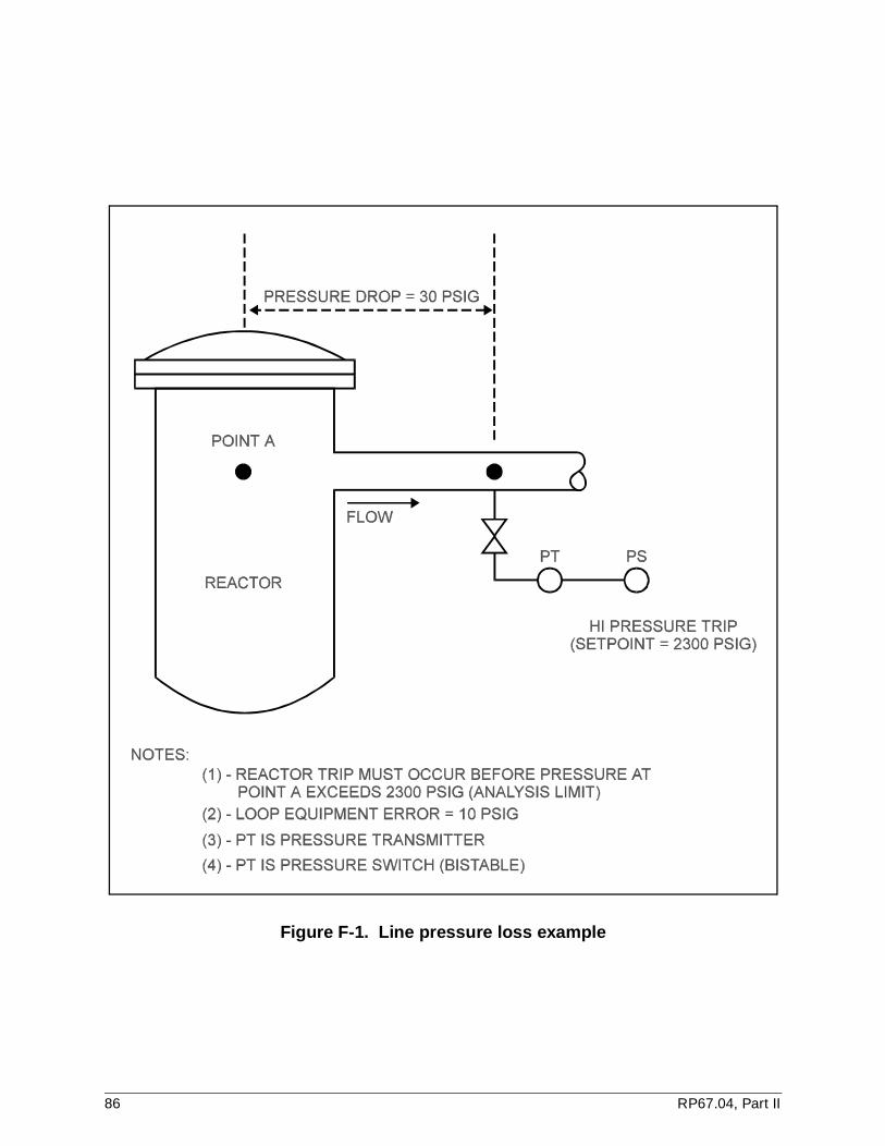
Figure F-1. Line pressure loss example

86 RP67.04, Part II

Appendix G: RTD accuracy confirmation

The accuracy of an RTD can be confirmed using several different approaches. The ease of useand feasibility of each is dependent on the type of RTD installation. The four approaches incommon use today are

a) comparison against a standard in a controlled environment; i.e., temperature bath;

b) normalization against a standard in a semicontrolled environment; i.e., during significant plant temperature changes (heatup or cooldown);

c) cross-calibration (or self-normalization) of a significant number of RTDs during plant temperature changes; and

d) replacement of the RTDs with factory-calibrated units.

There may be a shift in the accuracy of the calibration curve of the device if a mechanical shockis received before or during installation. The accuracy of the platinum-lead RTDs generally usedis based on a strain-free condition. Exposure to a mechanical shock severe enough to introducea change in this condition can invalidate the assumption that the device is calibrated to a finetolerance. Therefore, extreme care should be taken in the treatment of these devices to assurethat the calibration curve determined at the factory before shipment is maintained. Approaches(b) and (c) minimize the handling of these devices and also gather data after installation. Thisallows the verification of the accuracy in situ. While approach (c) does not have an explicitcomparison against a traceable standard, the accuracy may be reasonable for setpointdetermination when a large enough sample is used.

In approach (b), replacement of one or more RTDs with factory-calibrated units allows thenormalization of the remaining RTDs against the replacement units. The data is taken during aplant heatup or cooldown, resulting in a semicontrolled environment; i.e., the system temperatureis known to the accuracy of the replacement units. The stability of the temperature during thegathering of data is a function of the plant equilibrium both from a real and a procedural point ofview (allowed temperature drift during the data gathering and potential stratification if the RTDsare not all in the same orientation). This approach decreases the number of RTDs replaced whencompared to approach (d) and results in a slightly higher uncertainty associated with verificationof the calibration curve. Approaches (a) and (d) result in a low uncertainty concerning theaccuracy of the devices, since they are calibrated under precise conditions. However, there is noin situ verification that the determined accuracy is valid after installation.

During the performance of RTD accuracy verification, the following items should be considered:

a) While it is not necessary to have a 0°F rate of change as a function of time, it is recommended that the rate of change be constant during the gathering of data.

b) Multiple data points for each RTD should be gathered at each temperature to reduce the uncertainty at that temperature.

c) Multiple temperature points should be used to verify the calibration curve in the range of interest and to minimize extrapolation errors.

d) Use a high accuracy readout device capable of compensating for lead wire imbalance.

RP67.04, Part II 87

e) All RTD lead combinations should be utilized during the verification process to allow use of the combination (either two, three, or four leads depending on the resistance to voltage or resistance to current conversion used in the instrument channel), which minimizes lead imbalance uncertainties. Any thermal EMF generated (from different metals at the lead junctions) should be considered when connecting the RTD to the electronics.

f) Leadwire resistance changes from environmental temperature variations should be considered for the two- and three-wire RTDs. This effect is a bias.

88 RP67.04, Part II

Appendix H: Uncertainties associated with digital signal processing

This appendix presents a discussion on digital signal processing and the uncertainties involvedwith respect to determining instrument channel setpoints for a digital system. Figure H-1presents a simplified block diagram of a digital processing system. The digital processor receivesan analog input signal and provides an output in either digital or analog form. Figure H-2 presentsa block diagram for the typical operations performed in the digital processor. Figure H-2 could berepresentative of process control computers, microcomputers, programmable controllers, etc.

The analog signal is received by the digital processor, filtered, digitized, manipulated, convertedback into analog form, filtered again, and sent out. The digital processor is treated as a black box;therefore, the discussion that follows is applicable to many different types of digital processors.The digital processor is programmed to run a controlled algorithm. Basic functions performed areaddition, subtraction, multiplication, and division as well as data storage. The digital processor isthe most likely component to introduce rounding and truncation errors.

The analog input signal is first processed by a filter to reduce aliasing noise introduced by thesignal frequencies that are high relative to the sampling rate. The filtered signal is sampled at afixed rate and the amplitude of the signal held long enough to permit conversion to a digital word.The digital words are manipulated by the processor based on the controlled algorithm. Themanipulated digital words are converted back to analog form, and the analog output signal issmoothed by a reconstruction filter to remove high frequency components.

Several factors affect the quality of the representation of analog signals by digitized signals. Thesampling rate affects aliasing noise; the sampling pulse width affects analog reconstructionnoise; the sampling stability affects jitter noise; and the digitizing accuracy affects thequantization noise.

H.1 Sampling rate uncertainty

If the sampling rate is higher than twice the analog signal bandwidth, the sampled signal is agood representation of the analog input signal and contains all of the significant information. Ifthe analog signal contains frequencies that are too high with respect to the sampling rate,aliasing uncertainty will be introduced. Anti-aliasing band-limiting filters can be used to minimizethe aliasing uncertainty or else it should be accounted for in setpoint calculations.

H.2 Signal reconstruction uncertainty

Some information is lost when the digitized signal is sampled and held for conversion back toanalog form after digital manipulation. This uncertainty is typically linear and about + 1/2 leastsignificant bit (LSB).

RP67.04, Part II 89

H.3 Jitter uncertainty

The samples of the input signal are taken at periodic intervals. If the sampling periods are notstable, an uncertainty corresponding to the sampled signal's rate-of-change will be introduced.The jitter uncertainty is insignificant if the clock is crystal-controlled, which it is in the majority ofcases.

H.4 Digitizing uncertainty

When the input signal is sampled, a digital word is generated that represents the amplitude of thesignal at that time. The signal voltage must be divided into a finite number of levels that can bedefined by a digital word "n" bits long. This word will describe 2n different voltage steps. Thesignal levels between these steps will go undetected. The digitizing uncertainty (also known asthe quantizing uncertainty) can be expressed in terms of the total mean square error voltagebetween the exact and the quantized samples of the signal. An inherent digitizing uncertainty of + 1/2 LSB typically exists. The higher the number of bits in the conversion process, the smallerthe digitizing uncertainty.

H.5 Miscellaneous uncertainties

Analog-to-digital converters also introduce offset uncertainty; i.e., the first transition may notoccur at exactly + 1/2 LSB. Gain uncertainty is introduced when the difference between thevalues at which the first transition and the last transition occur is not equal. Linearity uncertaintyis introduced when the differences between the transition values are not all equal.

For digital-to-analog conversion, the maximum linearity uncertainty occurs at full scale when allbits are in saturation. The linearity determines the relative accuracy of the converters. Deviationsfrom linearity once the converters are calibrated is absolute uncertainty. Power supply effectsmay also be considered for unregulated power supplies.

H.6 Truncation and rounding uncertainties

The effect of truncation or rounding depends on whether fixed point or floating point arithmetic isused and how negative numbers are represented and should be considered as a possibleuncertainty.

90 RP67.04, Part II

Figure H-1. Digital processing system simplified block diagram

Figure H-2. Digital processor block diagram

RP67.04, Part II 91

Annex I: Recommendations for inclusion of instrument uncertainties during normal operation in the allowable value determination

ISA-S67.04, Part I, 4.3.2, and ISA-RP67.04, Part II, 7.3, allow the use of instrument calibrationuncertainties, instrument uncertainties during normal operation, and instrument drift in thedetermination of the allowable value (AV). The instrument uncertainties during normal operationare listed in 4.3.1(b) of S67.04, Part I. However, it is not always appropriate to include all of theseuncertainties in the allowance between the AV and the trip setpoint (TS). The followingdiscussion provides recommendations for their inclusion in the determination of the AV.

Recall that the AV is a parameter to be used by the plant to verify channel performance atprescribed surveillance intervals. Therefore, of the uncertainties listed in S67.04, 4.3.1(b), onlythose associated with events expected to cause changes that would be discernible during thoseperiodic surveillances (as opposed to cycle recalibrations) should be included in the allowancebetween the AV and the TS.

When using the methods described in 7.3 or RP67.04, Part II, excluding any of these parametersfrom the allowance between the AV and the TS is conservative since the difference between theAL and the AV will increase. Thus, decreasing the difference between the TS and AV results in asmaller allowance for drift for the channel being tested. The following items should be consideredwhen determining whether or not to include the effects of each of these uncertainties in theallowance between the AV and TS (the numbers and titles refer to the associated paragraphs inS67.04, Part I):

4.3.1(b)1 - Reference accuracy

The "calibration accuracy" as described in RP67.04, Part II, 6.2.6, assumed the "tested"portion of the channel should be included in the allowance between the AV and TS. Thevarious device "calibration accuracies" should be combined in the same fashion whendetermining AV as when the "total error" was determined.

4.3.1(b)2 and 3 - Power supply voltage and frequency changes

These may be included if it is determined that their effects are significant and are likely tobe observed. Typically, however, these effects are small and are not usually measured, inwhich case, their inclusion in AV may be nonconservative.

4.3.1(b)4 - Temperature changes

If the temperature change expected to occur between periodic surveillances has acorresponding uncertainty that is significant, it may be included in the allowance betweenthe AV and TS. However, if the temperature at the time of the surveillance is expected tobe relatively constant with respect to the temperature change assumed in the setpointcalculation for the "tested" portion of the channel, the uncertainty due to temperaturechanges should not be included in this allowance.

EXAMPLE:

Suppose the temperature effects associated with the process electronics were assumed tobe ±1.0% span based on an assumed ambient temperature of 80°F ±30°F. If the processelectronics are located in an environment where the temperature is expected to bemaintained within a small band, ±3°F for instance, where the temperature effects are

RP67.04, Part II 93

negligible, it would not be necessary to include temperature effects in the allowancebetween the AV and TS. If, however, the process electronics were located in anuncontrolled environment, perhaps subject to swings in seasonal temperatures, and theseswings were expected to be significant, it would then be appropriate to consider includinguncertainties due to temperature effects when determining the allowance between the AVand TS.

4.3.1(b)5 - Humidity changes

See previous discussions on temperature.

4.3.1(b)6 - Pressure changes

See previous discussion on temperature.

4.3.1(b)7 - Vibration

Effects due to the in-service vibration, if expected to be significant between periodicsurveillances, may be considered for inclusion in the allowance between the AV and TS.

Effects due to seismic vibration, however, should not be included since seismic vibration isnot a normal occurrence between periodic surveillances.

4.3.1(b)8 - Radiation exposure

Effects due to radiation exposure during normal operation, if expected to be significantbetween periodic surveillances, may be considered for inclusion in the allowance betweenthe AV and TS.

4.3.1(b)9 - Analog-to-digital conversion

If analog-to-digital conversion is part of the "tested" portion of the channel, uncertaintiesdue to the A/D conversion should be included in the allowance between the AV and the TS.

94 RP67.04, Part II

Appendix J: Discussions concerning statistical analysis

J.1 Square root sum squares (SRSS) combination

The SRSS methodology for combining uncertainty terms that are random and independent is anestablished and accepted analytical technique. The SRSS methodology is a direct application ofthe central limit theorem, providing a method for determining the limits of a combination ofindependent and random terms. The probability that all the independent processes underconsideration would simultaneously be at their maximum value in the same direction (i.e., + or -)is very small. The SRSS methodology provides a means to combine individual randomuncertainty terms to establish a resultant net uncertainty term with the same level of probabilityas the individual terms. If an individual uncertainty term is known to consist of both random andbias components, the components should be separated to allow subsequent combination of likecomponents. Bias components should not be mixed up with random components during SRSSaddition.

Resultant net uncertainty terms should be determined from individual uncertainty terms basedon a common probability level. In some cases individual uncertainty terms may need to beadjusted to the common probability level. Typically, a probability level that corresponds to twostandard deviations (2 sigma) is used. Using probability levels that correspond to three or morestandard deviations may be unnecessarily conservative, resulting in reduced operating margin.For example, if a reference accuracy for a 99% probability level (3 sigma) is given as ±6 psig, the95% probability level corresponds to ±4 psig (= 2/3 x 6).

The central limit theorems require that the variables to be combined must be random andindependent. Some statements of the theorem allow individual variables to be either identically orarbitrarily distributed. Then, if the number of components, n, is large, the distribution of the sumwill be approximately normal. (See K.V. Bury and P.L. Meyer References). "Large" has beeninterpreted as 10-30. (See J.M. Hammersley Reference.) Another statement of the theoremrequires individual variables to be approximately normally distributed, and their variances aboutequal (none are dominant). If these conditions are met, the sum of the components will beapproximately normally distributed even for a relatively small n. "Relatively small" has beeninterpreted as low as 4. (See H.H. Ku Reference.) In the limiting case, if two individual variablesare exactly normal, their sum is exactly normal as well.

When a random variable represents the net effect of a large number of smaller, independent,unmeasurable causes, the variable can be expected to be approximately normally distributed.The approximation becomes better as the number of contributors increases. Empirical evidencesuggests that the normal distribution provides a good representation of many physical variables,including instrument uncertainties. This observation is consistent with the fact that mostinstrument channels are composed of several parts that contribute independent, randomuncertainties to the net sum. Even if the number of modules in a given instrument loop isrelatively small, the number of elemental uncertainty sources within the modules can be muchlarger, making the SRSS summation justifiable.

It should be noted that some random variables cannot be reasonably considered as the sum ofmany small uncertainties and, consequently, should not be expected to be normally distributed.For example, the predominance of one non-normal uncertainty within a sum may not allow the

RP67.04, Part II 95

sum to approximate normality. For such a case, the non-normal uncertainty is called abnormallydistributed and should be summed separately.

A different approach in the application of the SRSS technique is presented in ANSI/ASME PTC 19.1;the SRSS combination of biases is used and justified on the basis that all of the biases are random.The reader is cautioned that ANSI/ASME PTC 19.1 is intended for application to activities differentfrom the purpose of this recommended practice. However, there may be situations involving thecombination of significant numbers of random biases that could be treated by SRSS. The conditionsfor the use of the ANSI/ASME PTC 19.1 approach include the application of a bias concept thatdiffers from this recommended practice and the calculation of an uncertainty coverage interval thatdiffers from the confidence and tolerance intervals discussed in the next section.

J.2 Confidence and tolerance intervals

In the context of setpoint determination, nuclear plant engineering groups are likely to deal withthe numerical intervals from different sources. These include the analysis of field data by plantpersonnel and the use of manufacturer's specifications.

Field measurements at a plant can form the database for statistical analysis using knowntechniques. Normality tests and knowledge of sample sizes allow determining the closeness ofcommonly used approximations. These include normality and the closeness of estimators withtrue population parameters. The parameters population mean (µ) and standard deviation (sigma)are estimated by the sample mean (x) and standard deviation (s). This approximation is madebetter as the sample size increases.

If these approximations are taken, it is sufficient to describe a probability interval as a range ofvalues that includes (with a pre-assigned potential for occurrence called the confidence level) thetrue value of a population parameter. For a normal distribution, a ±1.96 s interval (approximately±1.96 sigma) has a 95% probability of including the true parameter. Another commoninterpretation is that 95% of the population is contained in the interval.

If a sample population is known to be small, it may be difficult to justify the above approximations,and it is appropriate to establish uncertainty limits using statistical tolerance intervals. Thisapproach requires the additional statement about the population proportion included in theinterval.

It is frequently desired to describe a tolerance interval using the sample mean and the samplestandard deviation such as x ± Ks. The value of K (tolerance factor) is a function of the samplesize, the confidence level, the population proportion, and whether the distribution is one-sided ortwo-sided. Tables of K values are given in A.H. Bowker and H.H. Ku References.

Numerical intervals also originate from manufacturer's product specifications. The ±Aspecification may represent a confidence interval (with a specified confidence level and animplicit assumption that estimators closely agree with population parameters) or a toleranceinterval (with specified confidence level, population proportion, and sample size). The correctinterpretation often requires discussion with the instrument manufacturer.

96 RP67.04, Part II

Appendix K: Propagation of uncertainty through signal-conditioning modules

This appendix discusses techniques for determining the uncertainty of a module's output whenthe uncertainty of the input signal and the uncertainty associated with the module are known.Using these techniques, equations are developed to determine the output uncertainties forseveral common types of functional modules.

For brevity, error propagation equations will not be derived for all types of signal-processingmodules. Equations for only the most important signal-processing functions will be developed.However, the methods discussed can be applied to functions not specifically addressed here.The equations derived are applicable to all signal conditioners of that type regardless of themanufacturer.

The techniques presented here are not used to calculate the inaccuracies of individual modules;they are used to calculate uncertainty of the output of a module when the module inaccuracy,input signal uncertainty, and module transfer function are known.

This section discusses only two classifications of errors or uncertainties: those that are randomand independent and can be combined statistically, and those that are biases and must becombined algebraically. The methods discussed can be used for both random and biaseduncertainty components.

It is important to note that the method of calibration or testing may directly affect the use of theinformation presented in this section. If, for example, all of the modules in the process electronicsfor a particular instrument channel are tested together, they may be considered one device. Theuncertainty associated with the output of that device should be equal to or less than theuncertainty calculated by combining all of the individual modules.

K.1 Error propagation equations using partial derivatives and perturbation techniques

Several valid approaches for the derivation of equations express the effect of passing an inputsignal with an error component through a module that performs a mathematical operation on thesignal. The approaches discussed here, which are recommended for use in developing error-propagation equations, are based on the use of partial derivatives (see C.S. Zalkind Reference)or perturbation techniques; i.e., changing the value of a signal by a small amount and evaluatingthe effect of the change on the output. Either technique is acceptable and the results, in mostcases, are similar.

For simplicity, this discussion assumes that input errors consist of either all random or all biaseduncertainty components. The more general case of uncertainties with both random and biasedcomponents is addressed later in this appendix.

RP67.04, Part II 97

K.2 Propagation of input errors through a summing function

The summing function is represented by the equation

c = k1 * A + k2 * B (Eq. K.1)

where k1 and k2 are constants that represent gain or attenuation of the input signals.

Accounting for input errors, the equation becomes

C + c = k1 * (A + a) + k2 * (B + b) (Eq. K.2)

where

A and B = inputs;

C = the output;

a, b, c = associated errors.

Subtracting Equation K.1 from Equation K.2 leaves

c = (k1 * a) + (k2 * b) (Eq. K.3)

This equation is appropriate for combining bias (systematic) errors.

If the errors are random; i.e., they can be combined by SRSS methods, the equation becomes

c(SRSS) = [(k1 * a)2 + (k2 * b)2]1/2 (Eq. K.4)

Using partial derivatives

δC/δA = δ(k1 * A)/δA + δ(k2 * B)/δA (Eq. K.5)

δC/δB = δ(k1 * A)/δB + δ(k2 * B)/δB (Eq. K.6)

which yields

δC = (δC/δA) * δA + (δC/δb) * δB

= k1 * dA + k2 * dB (Eq. K.7)

If δA = +a, δB = +b, and δC = +c

c = + (k1 * a) + (k2 * b) (Eq. K.8)

Again, using SRSS methods

δC = + [[(δC/δA) * a]2 + [(δC/δB) * b]2]1/2 (Eq. K.9)

from which

c(SRSS) = +[(k1 * a)2 + (k2 * b)2]1/2 (Eq. K.10)

Notice that in this case the same error propagation equations are obtained using either partialderivatives or perturbation techniques.

98 RP67.04, Part II

K.3 Propagation of input errors through a multiplication function

The equation for a multiplier is

C = (k1 * A) * (k2 * B) (Eq. K.11)

where k1 and k2 are linear gains or attenuation of the input signals.

Adding error terms yields

C + c = k1(A + a) * k2(B + b) (Eq. K.12)

which expands to

C + c = (k1 * A * k2 * B) + (k1 * A * k2 * b) + (k1 * a * k2 * B) + (k1 * a * k2 * b) (Eq. K.13)

Subtracting Equation K.11 from Equation K.13 yields

c = (k1 * A * k2 * b) + (k1 * a * k2 * B) + (k1 * a * k2 * b)

or

c = k1 * k2 * [+ (A * b) + (a * B) + (a * b)] (Eq. K.14)

This is more precise than the equation obtained from partial derivatives

c = k1 * k2 * [+(A * b) + (B * a)] (Eq. K.15)

The product of two or more error components; e.g., a * b, is small and may be ignored. They areincluded here to illustrate differences in the precision of calculations based on error propagationand calculations based on partial derivatives. In cases where there are many products of errors,it may be prudent to include them in the calculation and do the calculation on a computer.

Applying SRSS error combination to Equation K.14 yields

c(SRSS) = +k1 * k2 * [(A * b)2 + (B * a)2 + (a * b)2]1/2 (Eq. K.16)

The term (a * b)2 is extremely small and may be ignored. It is retained here for completeness.

Equation K.16 can be simplified further by expressing the errors in relative terms (c/C, a/A, b/B).The first order approximation of Equation K.16 is

c = +k1 * k2 * [+(A * b)2 +(a * B)2]1/2 (Eq. K.16a)

Squaring Equation K.16a and dividing by the square of Equation K.11 gives upon furtherreduction

c/C = [(a/A)2 + (b/B)2]1/2 (Eq. K.16b)

Several authors give simplified forms of error propagation equations for commonly usedfunctions. (See ANSI/ASTM E 178.)

K.4 Error propagation through other functions

Table 1 shows equations for other functions derived by the same techniques. Note that theseequations are useful only for determining the effect of a module on uncertainties in the inputsignal.

RP67.04, Part II 99

Using partial derivative techniques, suitable approximations can be derived from analyticaldescriptions (function f) of the transfer functions (or a Taylor series expansion) using the followinggeneral formula:

Random:

c = +[(δf / δa)2 * a2 + (δf / δb)2 * b

2]1/2

Bias (known sign):

c = (δf / δa) * a + (δf / δb) * b

Abnormal distribution or bias (unknown sign):

c = |(δf / δa) * a| + |(δf / δb) * b|

K.5 Accounting for module errors

K.5.1 Combining module errors with propagated input errors

So far we have dealt with the effects of a module's transfer function on inaccuracies oruncertainties present with the input signal. Besides affecting errors already present on inputsignals, each module contributes its own errors to the signals.

In the simplest case, where the module error can be represented by a single term, em, which isindependent of module and configuration, the error at the module output becomes

eo = +(eip + em) (Eq. K.17)

or

eo(SRSS) = +(eip2 + em

2)1/2 (Eq. K.18)

where

eip = propagated input error (see Figure K-1).

A more general case is illustrated in Figure K-2. The output of this module without errors is

Eo = {[(A) * (G1) + (B)] (G2)] * (G3)} (Eq. K.19)

Considering input error propagation and device and adjustment errors within the module, theequation for the output becomes

Eo + eo = {[(A + a) * (G1 + g1)+(B + b)](G2 + g2) + ez} * (G3 + g3) + em (Eq. K.20)

Subtracting Equation K.19 from Equation K.20 yields

eo = em + (A * G1 + B) * (G2 + g2) * (G3 + g3) + {[A * g1 + (a) * (G1 + g1) + (b)]

* (G2 + g2) + ez} * (G3 + g3) (Eq. K.21)

or

eo(SRSS) = + (em2 + (A * G1 + B) * (G2 + g2) * (G3 + g3)

+ {[A * g1 + (a) * (G1 + g1) + (b)] * (G2 + g2) + ez} * (G3 + g3)2)1/2 (Eq. K.22)

This error term would be the input signal error to the next module in the channel.

100 RP67.04, Part II

K.5.2 Quality of module error data

Error calculations are affected by how much module error data is available and by how it ispresented. Ideally, the magnitude, nature (random or bias), and source (drift, temperature effect,linearity, etc.) of each error component should be available. Error data should be traceable to thehardware vendor or to the independent test documentation.

Although most error terms are random, it is not prudent to assume that errors induced byaccident condition environments will not be systematic. Module errors may be estimated byanalysis. One useful technique is the Monte Carlo simulation. Four requirements for successfulsimulation are (1) the determination of sensitive components; i.e., those that have the greatestinfluence on accuracy; (2) product approximation of error distributions (Gaussian is usually themost accurate; uniform distribution is slightly more conservative; unusual distributions should beaccurately modeled); (3) generation of a sufficient number of simulated cases; and (4) verificationof the analysis by adequate testing.

K.6 Accounting for bias (systematic) error components

Although it is expected that most error components will be random and can be combined usingSRSS methods, bias error components must, at times, be dealt with. Perturbation techniques arewell-suited to handling combinations of bias and random error components. Calculations usingthese techniques will be at least as accurate as calculations using partial derivatives.

Using the multiplication functions as an example, the equation without errors is

C = A * B (Eq. K.23)

With errors it becomes

C + c = (A + a) * (B + b) (Eq. K.24)

If the a and b terms each contain both random and bias components, the equation becomes

C + c = (A + ar + ab) * (B + br + bb) (Eq. K.25)

where

ar, br = random components;

ab, bb = bias components.

Subtracting Equation K.23 from Equation K.25

c = +A * br +B * ar + ar * br + ar * bb + ab * br ±A * bb + B * ab + ab * bb (Eq. K.26)

The first five terms can be considered random because at least one member of each term is arandom error. These terms can be combined using SRSS. The last three terms consist only ofconstants and bias components and must be added algebraically. The final equation becomes

c = +[(A * br)2 + (B * ar)

2 + (ar * br)2 + (ar * bb)2 + (ab * br)

2]1/2 + A * bb + B * ab + ab * bb(Eq. K.27)

RP67.04, Part II 101

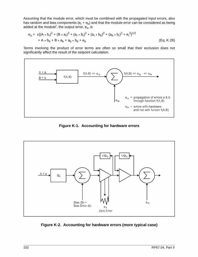
Assuming that the module error, which must be combined with the propagated input errors, alsohas random and bias components (er + eb) and that the module error can be considered as beingadded at the moduler, the output error, eo, is

eo = ±[(A * br)2 + (B * ar)

2 + (ar * br)2 + (ar * bb)2 + (ab * br)

2 + er2]1/2

+ A * bb + B * ab + ab * bb + eb (Eq. K.28)

Terms involving the product of error terms are often so small that their exclusion does notsignificantly affect the result of the setpoint calculation.

Figure K-1. Accounting for hardware errors

Figure K-2. Accounting for hardware errors (more typical case)

102 RP67.04, Part II

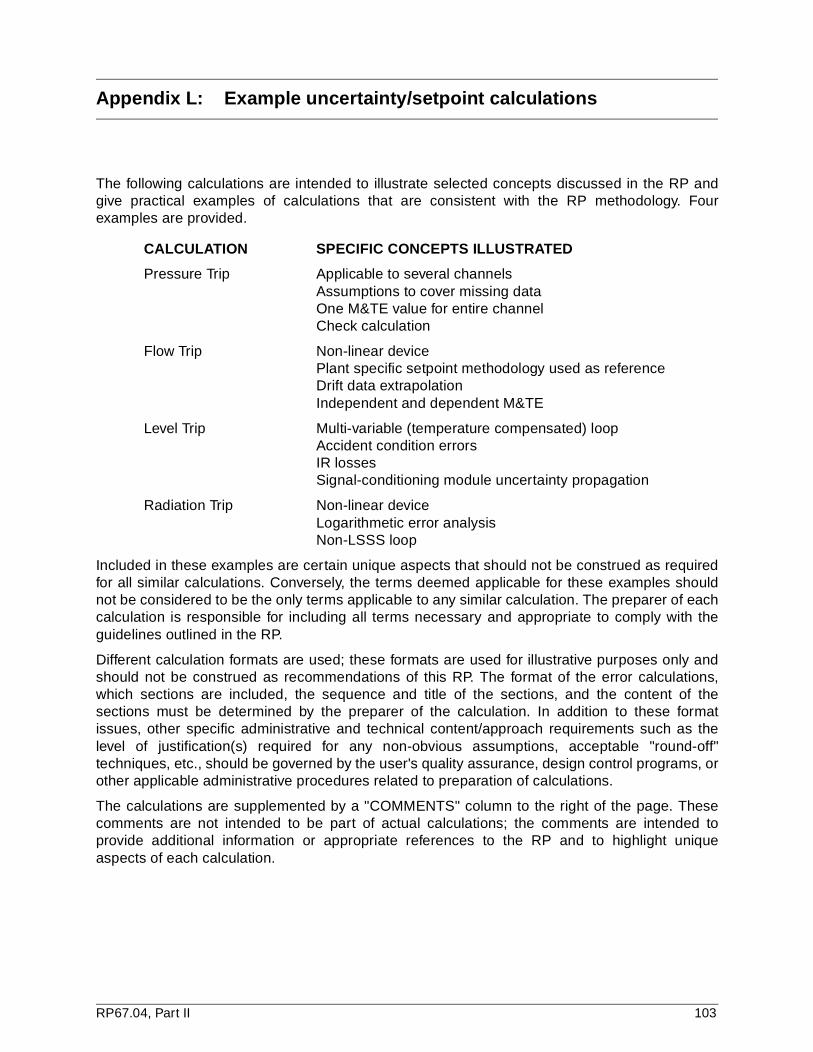
Appendix L: Example uncertainty/setpoint calculations

The following calculations are intended to illustrate selected concepts discussed in the RP andgive practical examples of calculations that are consistent with the RP methodology. Fourexamples are provided.

CALCULATION SPECIFIC CONCEPTS ILLUSTRATED

Pressure Trip Applicable to several channelsAssumptions to cover missing dataOne M&TE value for entire channelCheck calculation

Flow Trip Non-linear devicePlant specific setpoint methodology used as referenceDrift data extrapolationIndependent and dependent M&TE

Level Trip Multi-variable (temperature compensated) loopAccident condition errorsIR lossesSignal-conditioning module uncertainty propagation

Radiation Trip Non-linear deviceLogarithmetic error analysisNon-LSSS loop

Included in these examples are certain unique aspects that should not be construed as requiredfor all similar calculations. Conversely, the terms deemed applicable for these examples shouldnot be considered to be the only terms applicable to any similar calculation. The preparer of eachcalculation is responsible for including all terms necessary and appropriate to comply with theguidelines outlined in the RP.

Different calculation formats are used; these formats are used for illustrative purposes only andshould not be construed as recommendations of this RP. The format of the error calculations,which sections are included, the sequence and title of the sections, and the content of thesections must be determined by the preparer of the calculation. In addition to these formatissues, other specific administrative and technical content/approach requirements such as thelevel of justification(s) required for any non-obvious assumptions, acceptable "round-off"techniques, etc., should be governed by the user's quality assurance, design control programs, orother applicable administrative procedures related to preparation of calculations.

The calculations are supplemented by a "COMMENTS" column to the right of the page. Thesecomments are not intended to be part of actual calculations; the comments are intended toprovide additional information or appropriate references to the RP and to highlight uniqueaspects of each calculation.

RP67.04, Part II 103

EXAMPLE CALCULATION — PRESSURE TRIP

CALCULATION COMMENTS

1.0 Purpose

The purpose of this calculation is to determine if the setpoint that has been established as part of the NSSS Standard Technical Specifications (Reference 3.1) is appropriate for the specific application at Nuclear Plant Unit #2.

Note: The following format is for illustrative purposes only. See RP Preface, Section 10, and Page 103.

The specific application included in this calculation is for the Containment High Pressure Trip into the Steamline Isolation Logic. This calculation is required since the equipment suppliers for these components for Nuclear Plant Unit #2 are different than the equipment suppliers assumed by the NSSS.

This calculation is being prepared to comply with our commitments to Reg. Guide 1.105 (Reference 3.2) as outlined in FSAR Section 1.8 (Reference 3.3). In addition this calculation has been prepared to be consistent with the methodology out-lined in ISA-S67.04 (Reference 3.4).

2.0 Assumptions

2.1 There are no known bias or dependent uncertainty for any of the modules involved in this application (based on review of References 3.8, 3.9, and 3.10).

RP Sections 5.2 and 5.3 were reviewed to identify potentially applicable factors.

2.2 M&TE uncertainty for applications similar to that outlined in this calculation have been standardized at ±0.5% of process span (based on Reference 3.7.f).

See RP Section 6.2.6.

2.3 Final values of calculations will be rounded-off to achieve a consistent calculation degree of accuracy.

See Page 105. In this example, the final value for Eq. 6 - Eq. 13 has been adjusted to the nearest 0.1 unit.

2.4 A margin of 1.0 psig has been applied to the total channel uncertainty (based on Reference 3.7.g).

See RP Section 9. Reflects interface with other organizations.

2.5 A local temperature transient effect value for the pressure transmitter has been assumed to be ±1.0% U.R.L. (See Calcula-tion Sections 7.0 and 11.0.)

3.0 References

3.1 NSSS Technical Report 1234, Revision B, "Standard Techni-cal Specifications for Three-Loop Pressurized Water Reactors."

RP67.04, Part II 105

CALCULATION COMMENTS

3.2 U.S. Nuclear Regulatory Commission, Regulatory Guide 1.105, Revision 2, February 1986, "Instrument Setpoints for Safety-Related Systems."

3.3 Nuclear Plant Unit, Final Safety Analysis Report, Revision O.

a. Section 1.8, Conformance to NRC Regulatory Guides

b. Section 3.11, Environmental Qualification of Mechanical and Electrical Equipment

c. Section 6.2, Containment Systems

d. Section 7.0, Instrumentation and Controls

e. Section 15.0, Accident Analyses

3.4 ANSI/ISA-S67.04-1987, "Setpoints for Nuclear Safety-Related Instrumentation."

3.5 ISA-dRP67.04, Part II, Draft 7, "Methodologies for the Determination of Setpoints For Nuclear Safety-Related Instrumentation."

3.6 Nuclear Plant Unit #2, Drawings

a. P&ID, P-01, Rev. 3

b. Instrument Location, I-01, Rev. 2

c. Electrical Loop Schematic, E-01, Rev. 4

d. Plant Location, L-01, Rev. 1

3.7 Nuclear Plant #2 Documents

a. Calibration Procedure C-01, Rev. 0., Safety-Related Pressure Loops

b. Component Data Sheet (PT-MS-01), Issue 0

c. Component Data Sheet (PSL-MS-01), Issue 0

d. Test & Measurement Record, PI Serial #123

e. Test & Measurement Record, DVM Serial #456

f. Engineering Evaluation, EE-008, Rev. 0, "M&TE" Effects on Selected Applications

g. PORC Meeting Minutes for 1/4/88

3.8 Precise Pressure Company Product Literature

a. Pressure Transmitter Literature

b. DVM Literature

c. Pressure Gauge Literature

106 RP67.04, Part II

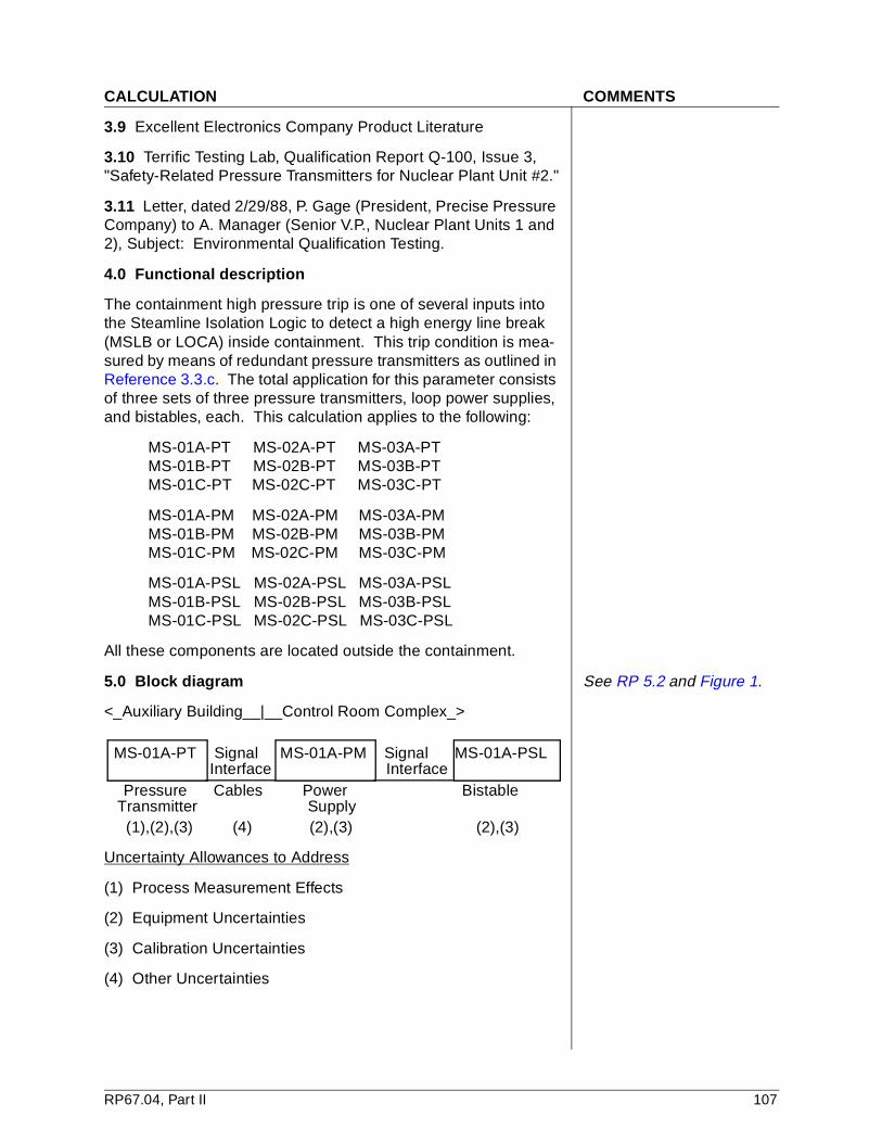
CALCULATION COMMENTS

3.9 Excellent Electronics Company Product Literature

3.10 Terrific Testing Lab, Qualification Report Q-100, Issue 3, "Safety-Related Pressure Transmitters for Nuclear Plant Unit #2."

3.11 Letter, dated 2/29/88, P. Gage (President, Precise Pressure Company) to A. Manager (Senior V.P., Nuclear Plant Units 1 and 2), Subject: Environmental Qualification Testing.

4.0 Functional description

The containment high pressure trip is one of several inputs into the Steamline Isolation Logic to detect a high energy line break (MSLB or LOCA) inside containment. This trip condition is mea-sured by means of redundant pressure transmitters as outlined in Reference 3.3.c. The total application for this parameter consists of three sets of three pressure transmitters, loop power supplies, and bistables, each. This calculation applies to the following:

MS-01A-PT MS-02A-PT MS-03A-PT MS-01B-PT MS-02B-PT MS-03B-PT MS-01C-PT MS-02C-PT MS-03C-PT

MS-01A-PM MS-02A-PM MS-03A-PM MS-01B-PM MS-02B-PM MS-03B-PM MS-01C-PM MS-02C-PM MS-03C-PM

MS-01A-PSL MS-02A-PSL MS-03A-PSL MS-01B-PSL MS-02B-PSL MS-03B-PSL MS-01C-PSL MS-02C-PSL MS-03C-PSL

All these components are located outside the containment.

5.0 Block diagram See RP 5.2 and Figure 1.

<_Auxiliary Building__|__Control Room Complex_>

MS-01A-PT Signal MS-01A-PM Signal MS-01A-PSL Interface Interface Pressure Cables Power Bistable Transmitter Supply (1),(2),(3) (4) (2),(3) (2),(3)

Uncertainty Allowances to Address

(1) Process Measurement Effects

(2) Equipment Uncertainties

(3) Calibration Uncertainties

(4) Other Uncertainties

RP67.04, Part II 107

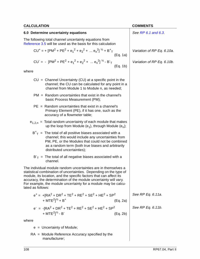
CALCULATION COMMENTS

6.0 Determine uncertainty equations See RP 6.1 and 6.3.

The following total channel uncertainty equations from Reference 3.5 will be used as the basis for this calculation

CU+ = + [PM2 + PE2 + e12 + e2

2 + ... en2] ½ + B+

T (Eq. 1a)

Variation of RP Eq. 6.10a.

CU- = - [PM2 + PE2 + e12 + e2

2 + ... en2] ½ - B-

T (Eq. 1b)

Variation of RP Eq. 6.10b.

where

CU = Channel Uncertainty (CU) at a specific point in the channel; the CU can be calculated for any point in a channel from Module 1 to Module n, as needed;

PM = Random uncertainties that exist in the channel's basic Process Measurement (PM);

PE = Random uncertainties that exist in a channel's Primary Element (PE), if it has one, such as the accuracy of a flowmeter table;

e1,2,n = Total random uncertainty of each module that makes up the loop from Module (e1), through Module (en);

B+T = The total of all positive biases associated with a

channel; this would include any uncertainties from PM, PE, or the Modules that could not be combined as a random term (both true biases and arbitrarily distributed uncertainties);

B-T = The total of all negative biases associated with a

channel.

The individual module random uncertainties are in themselves a statistical combination of uncertainties. Depending on the type of module, its location, and the specific factors that can affect its accuracy, the determination of the module uncertainty will vary. For example, the module uncertainty for a module may be calcu-lated as follows:

e+ = +[RA2 + DR2 + TE2 + RE2 + SE2 + HE2 + SP2

+ MTE2]½ + B+ (Eq. 2a)

See RP Eq. 6.11a.

e- = -[RA2 + DR2 + TE2 + RE2 + SE2 + HE2 + SP2

+ MTE2]½ - B- (Eq. 2b)

See RP Eq. 6.11b.

where

e = Uncertainty of Module;

RA = Module Reference Accuracy specified by the manufacturer;

108 RP67.04, Part II

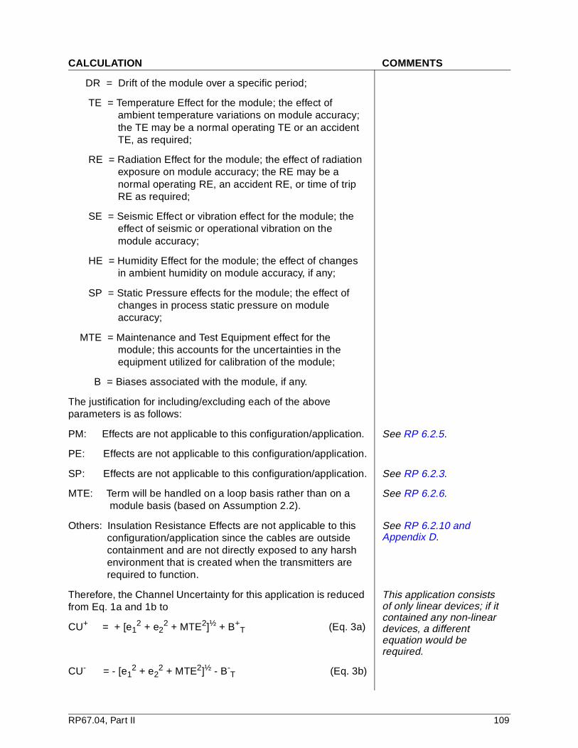
CALCULATION COMMENTS

DR = Drift of the module over a specific period;

TE = Temperature Effect for the module; the effect of ambient temperature variations on module accuracy;the TE may be a normal operating TE or an accidentTE, as required;

RE = Radiation Effect for the module; the effect of radiationexposure on module accuracy; the RE may be a normal operating RE, an accident RE, or time of tripRE as required;

SE = Seismic Effect or vibration effect for the module; theeffect of seismic or operational vibration on the module accuracy;

HE = Humidity Effect for the module; the effect of changesin ambient humidity on module accuracy, if any;

SP = Static Pressure effects for the module; the effect ofchanges in process static pressure on module accuracy;

MTE = Maintenance and Test Equipment effect for the module; this accounts for the uncertainties in theequipment utilized for calibration of the module;

B = Biases associated with the module, if any.

The justification for including/excluding each of the above parameters is as follows:

PM: Effects are not applicable to this configuration/application. See RP 6.2.5.

PE: Effects are not applicable to this configuration/application.

SP: Effects are not applicable to this configuration/application. See RP 6.2.3.

MTE: Term will be handled on a loop basis rather than on amodule basis (based on Assumption 2.2).

See RP 6.2.6.

Others: Insulation Resistance Effects are not applicable to thisconfiguration/application since the cables are outside containment and are not directly exposed to any harshenvironment that is created when the transmitters arerequired to function.

See RP 6.2.10 and Appendix D.

Therefore, the Channel Uncertainty for this application is reduced from Eq. 1a and 1b to

This application consists of only linear devices; if it contained any non-linear devices, a different equation would be required.

CU+ = + [e12 + e2

2 + MTE2]½ + B+T (Eq. 3a)

CU- = - [e12 + e2

2 + MTE2]½ - B-T (Eq. 3b)

RP67.04, Part II 109

CALCULATION COMMENTS

7.0 Determine uncertainty data

The following applies to the pressure transmitter (MS-01A-PT), and all appropriate terms will be designated with a subscript of 1; i.e., e1, RA1, etc.

RA1 = ±1% of Span (based on References 3.7.a and b) See RP 6.2.6.

DR1 = ±0.1% of Upper Range Limit (based on References 3.7.a and b)

See RP 6.2.7.

TE1 , RE1 , SE1 , and HE1 = See RP 6.2.2 and 6.2.4.

Specific values are not provided by the manufacturer in Reference 3.8.a. However, References 3.8.a and 3.10 have established a conservative value of ±5% of Upper Range Limit that includes all these effects for post-accident conditions. Pressure transmitters for this application are located outside containment (Reference 3.6) and, therefore, are not subjected to the in-containment environment when required to operate. However, the ±5% value has been included as a conservative factor to account for any possible environmental effects of the high energy line break inside containment effecting these transmitters in the auxiliary building. For this calculation, the term will be designated as EE1. Correspondence with the manufacturer (Reference 3.11) confirms that the manufacturer did test a sufficient number of samples to justify that the ±5% value is a random term.

See RP 6.2.4, 6.3.1, and Appendix J.

In addition to the terms outlined in Eq. 2, the transmitter can be affected by loop power supply variations. Therefore, a term (PS1) is required.

See RP 6.2.8.

PS1 = ±0.01% span per volt variation (based on References 3.7.b and 3.8.a).

Maximum voltage variation = ±2 volts (based on Reference 3.9).

B+1 , B-

1 = 0 (based on Assumption 2.1).

Therefore, e1 = ± [RA12 + DR1

2+ EE12 + PS1

2 ]½ (Eq. 4)

based on Reference 3.7.b, span = 0 - 75 psig U.R.L. = 100 psig

e1 = ±[ (0.01 x 75)2 + (0.001 x 100)2 + (0.05 x 100)2

+ (0.0001 x 2 x 75)2]½ psig = ±[25.57]½

= ±5.06 ≈ ±5.1 psig (Eq. 5)

110 RP67.04, Part II

CALCULATION COMMENTS

The following applies to the bistable (MS-01A-PSL) and all appropriate terms will be designated with a subscript of 2; i.e., e2, RA2 , etc.

RA2 = ±0.25% of span (based on References 3.7.c and 3.9).

DR2 = ±0.25% of span (based on References 3.7.a and 3.9).

TE2 = ±.02% span per 100°F (based on Reference 3.9).

Temperature Change = 50°F (based on Reference 3.3.b).

RE2 , SE2 , & HE2 : Effects are not applicable to this module (based on module location and

Reference 3.3.b).

In addition to the terms outlined in Eq. 2, this module can be affected by loop power supply variations. Therefore, a term (PS2) is required.

PS2 = ±0.01% span per Volt Variation (based on Reference 3.9).

Maximum Voltage Variation = ± 2 Volts (based on Reference 3.9).

Therefore, e2 = ±[RA22 + DR2

2 + TE22 + PS2

2 ]½ (Eq. 6) based on References 3.7.b and c,

Span = 0 - 75 psig.

e2 = ± [ (0.0025 x 75)2 + (0.0025 x 75)2 + (0.0002 x

{50/100} x 75)2 + (0.0001 x 2 x 75)2 ]½ psig

e2 = ± [0.071]½ = ±0.27 ≈ ±0.3 psig (Eq. 7)

8.0 Calculate instrument channel uncertainty See RP 6.3.

Based on the justification and data outlined in Section 7.0; i.e., B+

T = 0 and B-T = 0, the Channel Uncertainty equations (Eq. 3a

and 3b) for this calculation become

CU = ±[e12 + e2

2 + MTE2 ]½ (Eq. 8)

e1 = ±5. 1 psig (From Eq. 5) e2 = ±0.3 psig (From Eq. 7)

MTE = ±0.5%

Span = ± (0.005 x 75) = ±0.375 ≈ ±0.4 psig (Eq. 9)

CU = ±[ (5.1)2 + (0.3)2 (0.4)2 ]½

= ±[26.26]½ = ±5.12 ≈ ±5.1 psig (Eq. 10)

9.0 Obtain Analytical Limit (AL)

Per References 3.7.b and c, the loop range is 0-75 psig. See RP Section 7.0

Per References 3.3.c and e, Steamline Isolation is assumed to occur at 25 psig.

RP67.04, Part II 111

CALCULATION COMMENTS

10.0 Determine setpoint (TS) See RP Section 7.0

A nominal trip setpoint can be calculated as follows:

TS = AL ±(CU + Margin) See RP 7.2 & Eq. 7.1.

A Margin of 1.0 psig will be used (based on Reference 3.7.g).

Margin established as part of Interfaces discussed in RP Section 9.

Therefore, TS = 25 - (5.1 + 1.0) = 18.9 psig (Eq. 11)

(Note: The positive value of CU is not used to determine TS for an increasing parameter, since the process is increasing towards the analytical limit.)

11.0 Determine allowable value (AV) See RP Section 7 and Appendix I.

The uncertainties to be included in determining the Allowable Value are defined in Reference 3.4, Section 4.3.2. For this calculation, the only uncertainty that would be excluded from the CU are the uncertainties associated with design-basis events. However, as outlined in Section 7.0 of this calculation, a specific TE (for the transmitter) is not available from the manufacturer. Therefore, a value of TE1 = ±1.0% U.R.L. will be used to account for possible uncertainty due to temperature effects during normal operation.

Therefore, an Allowable Value Trip Setpoint Margin (AVTSM) can be calculated by modifying Eq. 4 to replace EE1 with TE1 and then combining the result with Eq. 7 and the MTE uncertainty.

See RP 7.3.

em = e1 (modified) = ±[RA12 + DR1

2 + TE12 + PS1

2 ]½ (Eq. 12)

= ±[(0.01 x 75)2 + (0.001 x 100)2 + (0.01 x 100)2

+ (0.0001 x 2 x 75)2]½ psig

= ±[1.57]½ = ±1.25 ≈ ±1.3 psig

AVTSM = ±[ em2 + e2

2 + MTE2 ]½ (Eq. 13)

= ±[ (1.3)2 + (0.3)2 + (0.4)2 ]½ psig

= ±[ 1.94]½ = ±1.39 ≈ ±1.4 psig

Based on Eq. 11 and Eq. 13,

AV = TS ± AVTSM = 18.9 + 1.4 = 20.3 psig. (Eq. 14) See RP 7.3.

(Note: Only the positive value of AVTSM is used to determine AV for an increasing parameter.)

112 RP67.04, Part II

CALCULATION COMMENTS

12.0 Check calculation See RP 7.3.

A check calculation will be performed to assure that the differ-ence between the allowable value and analytical limit is still large enough to account for those uncertainties not included in the test and to ensure that the safety limit is not exceeded by a worst case design-basis event.

If RP7.3 Method 3 is used, performing a check calculation is suggested to confirm that sufficient allowance exists between the AL and AV. This section of the calculation illustrates this technique. The RP recommends that this check calculation be performed if your AV is determined by using an arithmetic (versus an SRSS) approach. If your AV is determined by using an SRSS approach, the check calculation is not needed and is optional since it only increases the level of conservatism.

AVALM1 = (CU2 - AVTSM2)½

AVALM2 = |(AL - TS)| – |AVTSM|

where

AVALM1 = The required margin between the analytical limit and the allowable value;

If AVALM1 > AVALM2, then the allowable value is adjusted accordingly. Also, if the AVTSM is small (i.e., does not allow a realistic allowance for instrument drift), the nominal trip setpoint may be conservatively adjusted to minimize the chance of a Licensing Event Report (LER).

AVALM2 = The available margin between the analytical limit and the allowable value;

AVTSM = Allowable value trip setpoint margin;

CU = Channel uncertainty;

AL = Analytical limit;

TS = Nominal trip setpoint.

Based on Eq. 10 and Eq. 13

AVALM1 = [(5.1)2 - (1.4)2] ½ psig = [24.05]½ = 4.9 psig (Eq. 15)

Based on Section 9.0, Eq. 11, and Eq. 13,

AVALM2 = |(25-18.9)| – |(1.4)| psig = 4.7 psig (Eq. 16)

AVALM1 > AVALM2; therefore, TS and AV will be recalculated (adjusted) as follows:

AVadj = AL - AVALM1 (Eq. 17)

TSadj = AVadj - AVTSM (Eq. 18)

RP67.04, Part II 113

CALCULATION COMMENTS

Based on Section 9.0 and Eq. 15, Eq. 17 becomes

AVadj = (25) - (4.9) psig = 20.1 psig

Based on Eq. 17 and Eq. 13, Eq. 18 becomes

TSadj = (20.1) - (1.4) psig = 18.7 psig (Eq. 19)

13.0 Summary

Table 3.5-4 of Reference 3.1 outlines the following values for Containment High Pressure Trip for Steamline Isolation Logic.

Trip Setpoint: 18.5 psig

Allowable Value: 20 psig

Therefore, the use of Reference 3.2 and 3.4 methodology for the specific components being used at Nuclear Plant Unit #2 con-firms that this installation is consistent with the Standard Tech Spec values, and use of the Standard Tech Spec setpoint and allowable values is conservative.

114 RP67.04, Part II

EXAMPLE CALCULATION — FLOW TRIP

CALCULATION COMMENTS

1.0 Purpose NOTE: The following format is for illustrative purposes only. See RP Preface, Section 10, and Page 105.

To calculate a setpoint for the feedwater flow isolation trip. This calculation will support the installation of the components listed in Section 5 during the December 1990 refueling outage per Design Change Package 90-01.

2.0 Assumptions and clarifications RP 5.2 and 5.3 were reviewed to identify poten-tially applicable factors.

2.1 The calculation will assume all components perform as designed. This assumption leads to the following results: in a current loop series, components do not affect loop current, since current is constant at all points in a current loop.

2.2 In the operating ranges of interest (450o to 480oF and 400 to 450 psig) changes in water density due to changes in temperature and pressure are too small to affect channel accuracy.

Addresses RP Appendix C concerns.

2.3 Plant Procedure STD-0001, Methodology for Calculating Setpoints, is the basis for the uncertainty combinations and setpoint determinations in this calculation.

2.4 Drift is extended from the tested interval to the calibration interval using a SRSS technique, such that the drift is multiplied by the square root of the ratio of the calibration interval to the test interval.

2.5 Some manufacturer data is given in percent reading. This will be conservatively increased to percent full span to simplify the calculation, since in this application the process span is the same as the loop span.

2.6 The accuracy assigned to the flow element includes the effects of the installed piping configuration and effects of flow element degradation.

Addresses RP/Appendix C concerns.

RP67.04, Part II 115

CALCULATION COMMENTS

Line Pressure Loss/Head Pressure effects addressed in RP Appendix F are not applicable since point of measurement and point of concern are the same, and the flow element is installed in a horizontal section of pipe (Based on Reference 3.17).

2.7 Reference accuracy is the accuracy of the component under reference (ideal) conditions. Calibration accuracy is the accuracy to which the component is calibrated. This calculation will use the largest of the two values.

2.8 All loop components are located in areas where the environments are not affected by any accident. Therefore, no IR or other harsh environment effects are applicable. Also, based on References 3.4 - 3.7 and 3.10, the normal operating environmental variations are within the components specification values.

Insulation Resistance Effects addressed in RP Appendix D were determined not to be applicable based on Reference 3.16.

3.0 References

3.1 Station Drawing 1234567 Rev 8

3.2 Calibration Procedure CAL-001 for FW-01-F Feedwater Flow Loop, Revision 2, dated 6/6/89

3.3 (flow orifice product literature)

3.4 (dP transmitter product literature)

3.5 (power supply product literature)

3.6 (square root extractor product literature)

3.7 (bistable product literature)

3.8 (pressure gauge product literature)

3.9 (DVM product literature)

3.10 (Environmental levels for instrument locations)

3.11 STD-0001, Methodology for Calculating Setpoints

3.12 FSAR Table 1.1, Feedwater System Design Criteria

3.13 FSAR Table 1.2, Vital Bus Design Criteria

3.14 Feedwater System Design Criteria Document, Revision 0

3.15 Change Notice 123, Feedwater Transmitter Replacement

116 RP67.04, Part II

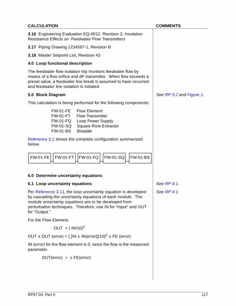
CALCULATION COMMENTS

3.16 Engineering Evaluation EQ-0012, Revision 3, Insulation Resistance Effects on Feedwater Flow Transmitters

3.17 Piping Drawing 1234567-1, Revision B

3.18 Master Setpoint List, Revision 43

4.0 Loop functional description

The feedwater flow isolation trip monitors feedwater flow by means of a flow orifice and dP transmitter. When flow exceeds a preset value, a feedwater line break is assumed to have occurred and feedwater line isolation is initiated.

5.0 Block Diagram See RP 5.2 and Figure 1.

This calculation is being performed for the following components:

FW-01-FE Flow Element FW-01-FT Flow Transmitter FW-01-FQ Loop Power Supply FW-01-SQ Square Root Extractor FW-01-BS Bistable

Reference 3.1 shows the complete configuration summarized below.

FW-01-FE FW-01-FT FW-01-FQ FW-01-SQ FW-01-BS

6.0 Determine uncertainty equations

6.1 Loop uncertainty equations See RP 6.1.

Per Reference 3.11, the loop uncertainty equation is developed by cascading the uncertainty equations of each module. The module uncertainty equations are to be developed from perturbation techniques. Therefore, use IN for "Input" and OUT for "Output."

See RP 6.1.

For the Flow Element,

OUT = ( IN/10)2

OUT ± OUT (error) = { [IN ± IN(error)]/10}2 ± FE (error)

IN (error) for the flow element is 0, since the flow is the measured parameter.

OUT(error) = ± FE(error)

RP67.04, Part II 117

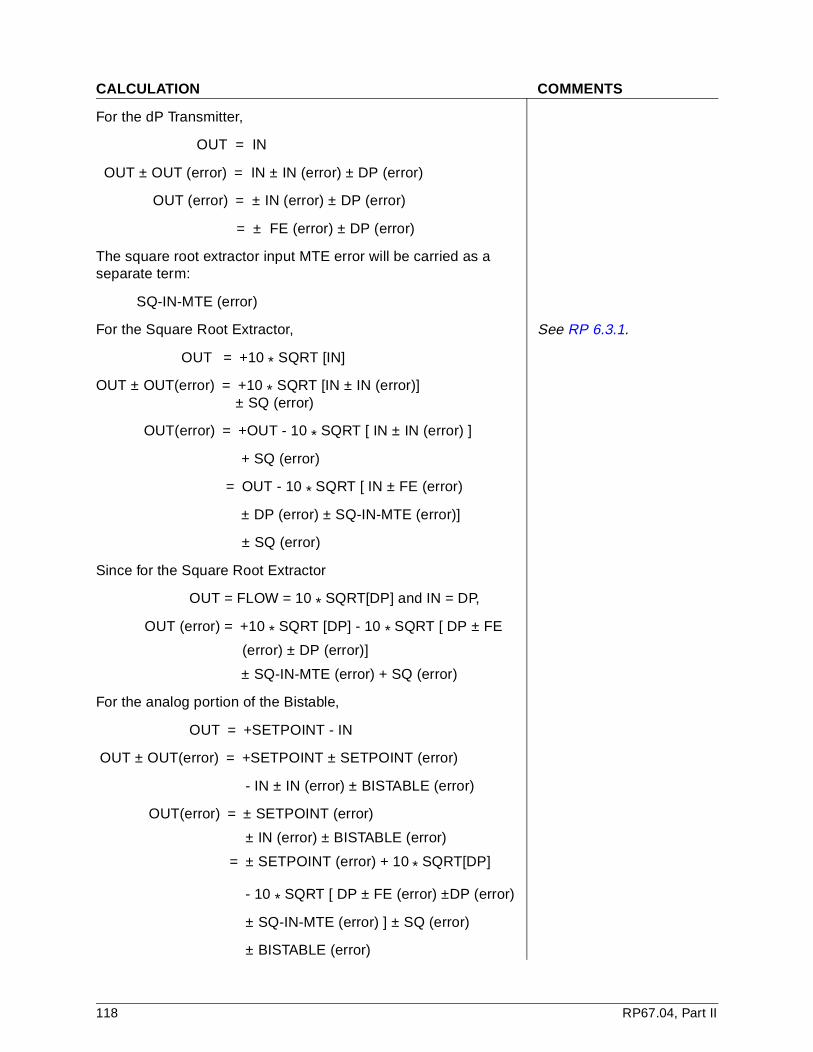
CALCULATION COMMENTS

For the dP Transmitter,

OUT = IN

OUT ± OUT (error) = IN ± IN (error) ± DP (error)

OUT (error) = ± IN (error) ± DP (error)

= ± FE (error) ± DP (error)

The square root extractor input MTE error will be carried as a separate term:

SQ-IN-MTE (error)

For the Square Root Extractor, See RP 6.3.1.

OUT = +10 * SQRT [IN]

OUT ± OUT(error) = +10 * SQRT [IN ± IN (error)] ± SQ (error)

OUT(error) = +OUT - 10 * SQRT [ IN ± IN (error) ]

+ SQ (error)

= OUT - 10 * SQRT [ IN ± FE (error)

± DP (error) ± SQ-IN-MTE (error)]

± SQ (error)

Since for the Square Root Extractor

OUT = FLOW = 10 * SQRT[DP] and IN = DP,

OUT (error) = +10 * SQRT [DP] - 10 * SQRT [ DP ± FE

(error) ± DP (error)]

± SQ-IN-MTE (error) + SQ (error)

For the analog portion of the Bistable,

OUT = +SETPOINT - IN

OUT ± OUT(error) = +SETPOINT ± SETPOINT (error)

- IN ± IN (error) ± BISTABLE (error)

OUT(error) = ± SETPOINT (error)

± IN (error) ± BISTABLE (error)

= ± SETPOINT (error) + 10 * SQRT[DP]

- 10 * SQRT [ DP ± FE (error) ±DP (error)

± SQ-IN-MTE (error) ] ± SQ (error)

± BISTABLE (error)

118 RP67.04, Part II

CALCULATION COMMENTS

Since the bistable is the last loop element, the bistable output uncertainty is the loop uncertainty.

CAVU = ± SETPOINT (error)

± (10 * SQRT [DP] See RP 6.1, Eq. 6.1; and 6.3, Eq. 6.10 a & b.

- 10 * SQRT [DP ± FE (error) ± DP (error)] )

± SQ (error) ± BISTABLE (error)

Per Reference 3.11, the random part of these terms may be combined by a SRSS technique, while the non-random part of these terms must be combined linearly. Therefore, both random and non-random components of each term will be determined.

6.2 Module Uncertainty Equations

Per Reference 3.11, the module uncertainty will address accuracy, ambient temperature effects, power supply variation effects, drift, and measurement and test equipment inaccuracy. In addition, module-unique effects should also be addressed.

Again, the random part of these terms may be combined by a SRSS technique, while the non-random part of these terms must be combined linearly. Therefore, both random and non-random components of each term will be determined.

7.0 Determine Uncertainty Data

7.1 Flow Element

Tag Number: FW-01-FE Reference 3.1Manufacturer: Ozzie Orifice Company Reference 3.3Model: ORF-001

See RP 6.2.

Reference Accuracy: ± 1.0 % of dp Reference 3.3Temperature Effect: 0 Assumption 2.2Pressure Effect: 0 Assumption 2.2Power Supply Effect: n/aDrift: n/aM&TE: n/a

Since there is only one non-zero term, FE (error) = ± 1.0 % span

7.2 Flow Transmitter

Tag Number: FW-01-FT Reference 3.1Manufacturer: Tommy Transmitter Co. Reference 3.4Model: FT-001Upper Range Limit: 1000 inches H2O Reference 3.4Span: 800 inches H2O Reference 3.2 See RP 6.2.6.

RP67.04, Part II 119

CALCULATION COMMENTS

Calibration Accuracy: ± 0.50 % span Reference 3.2Reference Accuracy: ± 0.25 % span Reference 3.4

Temperature Effect: ± 0.75 % URL / 100oF Reference 3.4Temperature Variation: ± 55oF Reference 3.10Temperature Effect: ± [(.75) (1000/800) (55/100)]Temperature Effect: ± 0.52 % span

See RP 6.2.2 & 6.2.4.

Pressure Effect: ± 0.20 % URL / 1000 psi Reference 3.4System Pressure: 425 psig Reference 3.12Pressure Effect: ± (0.2) (1000/800) (425/1000)Pressure Effect: ± 0.11 % span

See RP 6.2.3.

Power Supply Effect: ± 0.005 % span per volt Reference 3.4Voltage Variation: ± 1.0 volt Reference 3.5Power Supply Effect: (0.005) (1)Power Supply Effect: ± 0.005 % span

See RP 6.2.8.

Drift: ± 0.20 % URL / 6 months Reference 3.4Drift: ± (0.20) (1000/800) / 6 monthsDrift: ± 0.250 % span / 6 monthsCal Frequency: 18 months Reference 3.2Drift: ± 0.250 * SQRT [ 18/6 ]Drift: ± 0.433 % span

See RP 6.2.7.

M&TE: SQRT [Gage Error2 + DVM Error2] M&TE uncertainties of gage and I assumed random.

Gage Error: ± 0.1 % gage span Reference 3.8 Gage Span: 1000 inches H2O Reference 3.8 Gage Error: ± (0.1) (1000/800) Gage Error: ± 0.125 % span DVM Error: ± 0.02 % reading Reference 3.9 DVM Error: ± 0.02 % span Assumption 2.5

See RP 6.2.6.

M&TE: SQRT [ (0.125)2 + (0.02)2]M&TE: ± 0.127 % span

Since all the uncertainties are random, they can be combined by SRSS:

DP (error) = ± SQRT [ (0.5)2 + (0.52)2 + (0.11)2

+ (0.005)2 + (0.433)2 + (0.127)2 ]

DP (error) = ± 0.858 % span

120 RP67.04, Part II

CALCULATION COMMENTS

7.3 Square root extractor input mte error

M&TE:Input DVM Error: ± 0.02 % span Reference 3.9Input DVM Range: 20 volts Reference 3.9Input: 5 volts Reference 3.2Input DVM Error: ± (.02) (20/5)Input DVM Error: ± 0.08 % span

7.4 Square root extractor

Tag Number: FW-01-SQ Reference 3.1Manufacturer: Sammie SQRT Company Reference 3.6Model: SQRT-001

Calibration Accuracy: ± 0.65 % span Reference 3.2Reference Accuracy: ± 0.50 % span Reference 3.6

Temperature Effect: ± 0.05% span per 100oF Reference 3.6Temperature Variation: ± 20oF Reference 3.10Temperature Effect: ± (.05) (20/100)Temperature Effect: ± 0.01 % span

Pressure Effect: n/a

Power Supply Effect: ± 0.002 % span per % variation Reference 3.6

Voltage Variation: 118 ± 2 vac Reference 3.13Voltage Variation: ± 1.7 %Power Supply Effect: ± (.002) (1.7)Power Supply Effect: ± 0.004 % span

Final value of 0.004% is conservative round-off of actual value of 0.0034%.

Drift: ± 0.5 % per 18 months Reference 3.6Cal Frequency: 18 months Reference 3.2Drift: ± 0.5 % span

Output DVM Error: ± 0.02 % span Reference 3.9 Output DVM Range: 20 volts Reference 3.9 Output: 10 volts Reference 3.2 Output DVM Error: ± (.02) (20/10) Output DVM Error: ± 0.04 % span

Since all the uncertainties are random, they can be combined by SRSS.

SQ(error) = ± SQRT [ (0.65)2 + (0.01)2 + (0.004)2

+ (0.5)2 + (0.04)2 ]

SQ(error) = ± 0.821 % span

RP67.04, Part II 121

CALCULATION COMMENTS

7.5 Bistable

Tag Number: FW-01-BS Reference 3.1Manufacturer: Billie Bistable Company Reference 3.7Model: BIS-001

Calibration Accuracy: ± 0.1 % span Reference 3.2Reference Accuracy: ± 0.1 % span Reference 3.7

Temperature Effect: ± 0.02% span per 100oF Reference 3.7Temperature Variation: ± 20°F Reference 3.10Temperature Effect: ± (.02) (20/100)Temperature Effect: ± 0.004 % span

Pressure Effect: n/a

Power Supply Effect: ± 0.001 % span per % variation Reference 3.7

Voltage Variation: 118 ± 2 vac Reference 3.13Voltage Variation: ± 1.7%Power Supply Effect: ± (.001) (1.7)Power Supply Effect: ± 0.002 % span

Drift: ± 0.25 % per 18 months Reference 3.6Cal Frequency: 18 months Reference 3.2Drift: ± 0.25 % span

Input M&TE: Input DVM Error Input DVM Error: ± 0.02 % span Reference 3.9 Input DVM Range: 20 volts Reference 3.9 Input: 10 volts Reference 3.2 Input DVM Error: ± (.02) (20/10) Input M&TE Error: ± 0.04 % span

Since all the uncertainties are random, they can be combined by SRSS.

BISTABLE (error) = ± SQRT[ (0.1)2 + (0.004)2

+ (0.002)2 + (0.25)2 + (0.04)2 ]

BISTABLE (error) = ± 0.272 % span

7.6 Bistable setpoint

Calibration Accuracy: ± 0.10 % spanReference Accuracy: ± 0.05 % span

Temperature Effect: (included in bistable error)

Pressure Effect: n/a

Power Supply Effect: (included in bistable error)

122 RP67.04, Part II

CALCULATION COMMENTS

Stability (Drift): ± 0.02 % span/18 months Reference 3.7Calibration Period: 18 months Reference 3.2Stability: ± 0.02 % span

M&TE Error: Setpoint DVM Error DVM Error: ± 0.02 % input Reference 3.9 DVM Range: 20 volts Reference 3.9 Stpt Range: 10 volts Reference 3.2 M&TE Error: ± (.02) (20/10) M&TE Error: ± 0.04 % span

Since all the uncertainties are random, they can be combined by SRSS.

SETPOINT (error) = ± SQRT [ (0.1)2 + (0.02)2 + (0.04)2 ]

SETPOINT (error) = ± 0.110 % span

8.0 Calculate instrument channel uncertainty See RP 6.3.

From Section 7.0:

FE(error) = ± 1.000 % span DP(error) = ± 0.858 % span SQ-IN-MTE (error) = ± 0.08 % span SQ(error) = ± 0.829 % span

BISTABLE(error) = ± 0.272 % span

SETPOINT(error) = ± 0.110 % span

From Section 6.0:

CAVU = ± SETPOINT (error) + 10 * SQRT [DP]

- 10 * SQRT [ DP ± FE (error) ± DP (error)

± SQ-IN-MTE (error) ] ± SQ (error)

± BISTABLE (error)

Since the four terms

(1) SETPOINT (error);

(2) 10 * SQRT [DP] - 10 * SQRT [DP ± FE (error) ± DP (error) ± SQ-IN-MTE (error)];

(3) SQ(error); and

(4) BISTABLE (error)

are random and independent, they can be combined by an SRSS technique per Reference 3.11. For conservatism, FE (error), DP (error), and SQ-IN-MTE (error) will be added, although they could also be combined by an SRSS technique.

RP67.04, Part II 123

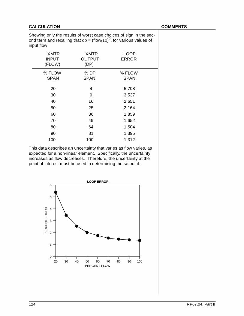
CALCULATION COMMENTS

Showing only the results of worst case choices of sign in the sec-ond term and recalling that dp = (flow/10)2, for various values of input flow

XMTR XMTR LOOP INPUT OUTPUT ERROR (FLOW) (DP)

% FLOW % DP % FLOW SPAN SPAN SPAN

20 4 5.708

30 9 3.537

40 16 2.651

50 25 2.164

60 36 1.859

70 49 1.652

80 64 1.504

90 81 1.395

100 100 1.312

This data describes an uncertainty that varies as flow varies, as expected for a non-linear element. Specifically, the uncertainty increases as flow decreases. Therefore, the uncertainty at the point of interest must be used in determining the setpoint.

6

5

4

3

2

1

0

20 30 40 50 60PERCENT FLOW

LOOP ERROR

70 80 90 100

124 RP67.04, Part II

CALCULATION COMMENTS

9.0 Obtain analytical limit See RP Section 7.

Per Reference 3.2, the loop range is 0 - 8000 gpm.

Per Reference 3.14, the maximum required feedwater flow during normal operation is 5000 gpm, and the maximum required feed-water flow during abnormal events and transients is 6500 gpm.

Per Reference 3.14, the pump run out flow rate (to atmosphere) is 8000 gpm.

10.0 Determine setpoint See RP Section 7 and Appendix I.

6500 gpm is approximately 80% flow. From the above, the loop uncertainty at 80% flow is approximately ± 1.5 % span or 120 gpm.

Minimum setpoint is 6500 gpm + 120 gpm = 6620 gpm.

8000 gpm is 100% flow. From the above, the loop uncertainty at 100% flow is approximately ± 1.3% span or 104 gpm.

Maximum setpoint is 8000 gpm - 104 gpm = 7896 gpm.

Per Reference 3.18, the existing in-plant setpoint is 7500 gpm. This is within the minimum and maximum bounds. Therefore, no change to the existing setpoint of 7500 gpm is recommended.

11.0 Determine allowable value

Per Reference 3.11, the allowable value is an estimate of loop performance including accuracy, drift, normal environmental effects, and M&TE, but not including harsh environmental effects. For this application, the allowable value will include accuracy, power supply effects, drift, and M&TE effects. Temperature and pressure are assumed to be at or very near calibration conditions.

The loop uncertainty equation does not change.

CAVU = ± SETPOINT (error)

± (10 * SQRT [DP] - 10 * SQRT [ DP ± FE (error)

± DP (error)] ) ± SQ (error) ± BISTABLE (error)

The module uncertainties become

FE (error) = ± 1.000 % span DP (error) = ± 0.674 % span SQ-IN-MTE (error) = ± 0.08 % span SQ (error) = ± 0.829 % span BISTABLE (error) = ± 0.272 % span SETPOINT (error) = ± 0.110 % span

RP67.04, Part II 125

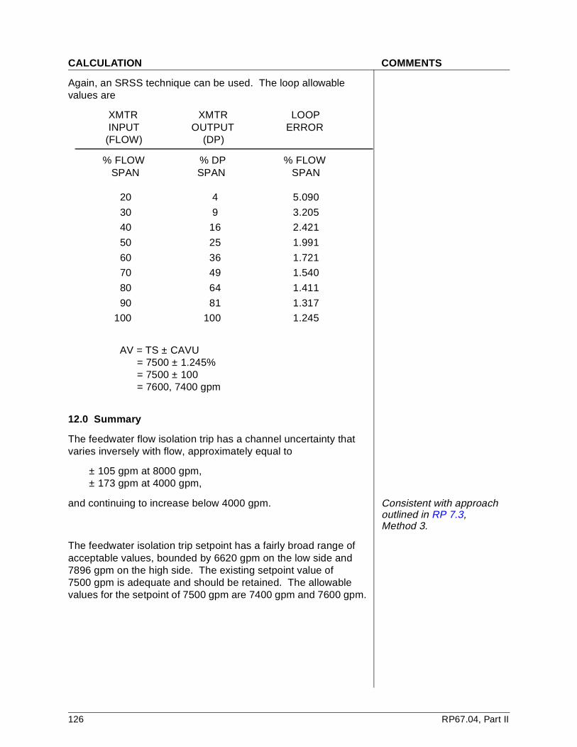
CALCULATION COMMENTS

Again, an SRSS technique can be used. The loop allowable values are

XMTR XMTR LOOP INPUT OUTPUT ERROR (FLOW) (DP)

% FLOW % DP % FLOW SPAN SPAN SPAN

20 4 5.090

30 9 3.205

40 16 2.421

50 25 1.991

60 36 1.721

70 49 1.540

80 64 1.411

90 81 1.317

100 100 1.245

AV = TS ± CAVU = 7500 ± 1.245% = 7500 ± 100 = 7600, 7400 gpm

12.0 Summary

The feedwater flow isolation trip has a channel uncertainty that varies inversely with flow, approximately equal to

± 105 gpm at 8000 gpm,± 173 gpm at 4000 gpm,

and continuing to increase below 4000 gpm. Consistent with approach outlined in RP 7.3, Method 3.

The feedwater isolation trip setpoint has a fairly broad range of acceptable values, bounded by 6620 gpm on the low side and 7896 gpm on the high side. The existing setpoint value of 7500 gpm is adequate and should be retained. The allowable values for the setpoint of 7500 gpm are 7400 gpm and 7600 gpm.

126 RP67.04, Part II

EXAMPLE CALCULATION - LEVEL TRIP

CALCULATION COMMENTS

1.0 Purpose NOTE: The following format is for illustrative purposes only. See RP Preface, Section 10, and Page 105.

This calculation will determine the instrumentation loop accuracies for the temperature-compensated pressurizer level reactor trip. This trip is required to operate for the first 15 minutes of a design-basis Main Stream Line Break (MSLB).

2.0 Assumptions RP 5.3 was reviewed to identify potentially applicable design parameters and sources of uncertainty.

2.1 The safety analyses show that the MSLB will produce little or no core damage. Therefore, the total integrated radiation dose to the cables and pressure transmitters in the first fifteen minutes will be small and will not affect their performance in this application.

2.2 Based on analyses contained in Reference 3.1, the pressurizer remains at saturation conditions throughout the MSLB accident scenario.

2.3 M&TE errors are bounded by plant requirements to be no greater than one-quarter (1/4) of the reference accuracy of the equipment being tested.

See RP 6.2.6.

2.4 Loop power supply is regulated to maintain voltage within the most limiting loop device's limitations.

2.5 There are no known dependencies between loop component error contributions. Therefore, all random uncertainties are treated as statistically independent.

2.6 Based on Reference 3.13:

a. Effects or vessel growth/contraction due to temperature changes are not included as they are estimated to be

insignificant to this application.

b. Changes in height of the reference leg due to vessel growth contraction are not included as they are estimated to be insignificant to this application.

3.0 References

3.1 East Fork Nuclear Generating Station UFSAR, Amendment 53.

3.2 East Fork Nuclear Generating Station Technical Specifications, Revision 12.

RP67.04, Part II 127

CALCULATION COMMENTS

3.3 East Fork Nuclear Generating Station Drawings

Control Loop Diagram RC-L001A, Revision 01

Process Protection Cable 1 1974-1000, Sheet 1, Revision 16

Process Instrument Cable 1 1974-1001, Sheet 2, Revision 11

Process Protection Cable 2 1974-1002, Sheet 1, Revision 13

Process Instrument Cable 2 1974-1003, Sheet 1, Revision 11

RCS Flow Diagram 1974-G-1020, Revision 27

Pressurizer Level Control Wiring Diagram B100-009, Revision 10

Pressurizer Level Control Wiring Diagram B100-010, Revision 13

Pressurizer Level Control Wiring Diagram B100-011, Revision 09

3.4 Delta-P Instrument Technical Manual #456789, Revision 2

3.5 ACME Engineering Specification for Class IE Transmitters, 1974-S395.15

3.6 ACME Engineering Specification for Process Analog Control System, 1974-S349.10

3.7 Instrument List, 1974-IL459, Revision 32

3.8 NSSS Owner's Group Report No. 0100, 100-101-3595, Revision 4

3.9 Cable Insulation Resistance Degradation Calculation EC-425-85, Revision 0

3.10 Pressurizer Level Transmitter Calibration Data Analysis 1974-6896, Revision 0

3.11 ANSI/ISA-S67.04, Setpoints for Nuclear Safety-Related Instrumentation, 1987

3.12 ISA-67.04, Part II, Methodologies for the Determination of Setpoints for Nuclear Safety-Related Instrumentation

3.13 RCS Measurement Channel Uncertainties Analysis, 1974-6867, Revision 00

4.0 Design Input Data

4.1 The Process Analog Control System cabinet components calibration uncertainty is ±2.5 % span based on a calibration tolerance of ±0.10 volts and a span of 4 volts. (Reference 3.8)

128 RP67.04, Part II

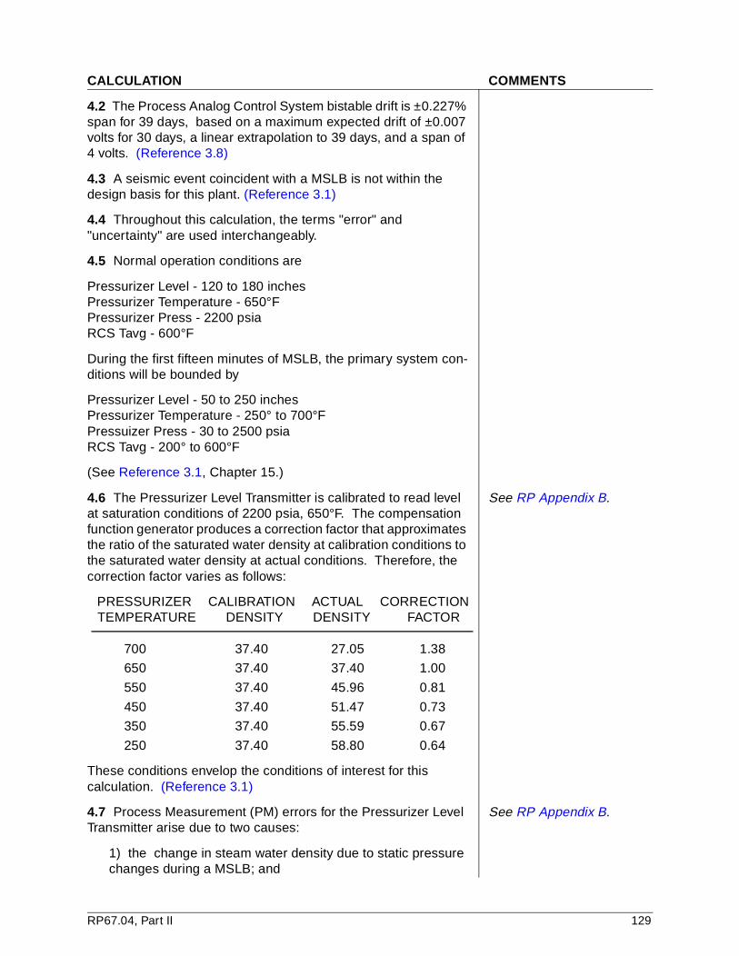
CALCULATION COMMENTS

4.2 The Process Analog Control System bistable drift is ±0.227% span for 39 days, based on a maximum expected drift of ±0.007 volts for 30 days, a linear extrapolation to 39 days, and a span of 4 volts. (Reference 3.8)

4.3 A seismic event coincident with a MSLB is not within the design basis for this plant. (Reference 3.1)

4.4 Throughout this calculation, the terms "error" and "uncertainty" are used interchangeably.

4.5 Normal operation conditions are

Pressurizer Level - 120 to 180 inchesPressurizer Temperature - 650°FPressurizer Press - 2200 psiaRCS Tavg - 600°F

During the first fifteen minutes of MSLB, the primary system con-ditions will be bounded by

Pressurizer Level - 50 to 250 inchesPressurizer Temperature - 250° to 700°FPressuizer Press - 30 to 2500 psiaRCS Tavg - 200° to 600°F

(See Reference 3.1, Chapter 15.)

4.6 The Pressurizer Level Transmitter is calibrated to read level at saturation conditions of 2200 psia, 650°F. The compensation function generator produces a correction factor that approximates the ratio of the saturated water density at calibration conditions to the saturated water density at actual conditions. Therefore, the correction factor varies as follows:

See RP Appendix B.

PRESSURIZER CALIBRATION ACTUAL CORRECTION TEMPERATURE DENSITY DENSITY FACTOR

700 37.40 27.05 1.38

650 37.40 37.40 1.00

550 37.40 45.96 0.81

450 37.40 51.47 0.73

350 37.40 55.59 0.67

250 37.40 58.80 0.64

These conditions envelop the conditions of interest for this calculation. (Reference 3.1)

4.7 Process Measurement (PM) errors for the Pressurizer Level Transmitter arise due to two causes:

See RP Appendix B.

1) the change in steam water density due to static pressure changes during a MSLB; and

RP67.04, Part II 129

CALCULATION COMMENTS

2) changes in reference leg density due to the reference leg heatup during a MSLB.

The change in static pressure during a MSLB. As noted above, Pressurizer pressure can shift from its nominal value of 2200 psia up to 2500 psia and down to 30 psia. These maximum changes of +300 psia and -2170 psia will cause errors of -0.15% process span and a +1.08% process span, respectively.

The reference leg heatup during the first 15 minutes of a MSLB will cause a +2.85% span error. (Reference 3.13)

Therefore, the PM for the Pressurizer Level Transmitter is +3.93% span, -0.15% span.

PMP = (+1.08 + 2.85) percent process span

PMN = -0.15% process span

4.8 PM error for the Pressurizer temperature RTD arises from temperature stratification in the pressurizer. To compensate for this effect, the Pressurizer temperature RTD was located at 80 inches, approximately halfway up the normal water column. Due to the dynamic changes occurring in the pressurizer because of pressure changes and temperature changes throughout the RCS, PM for the Pressurizer temperature RTD will be set to 0.0% span. (Reference 3.13)

5.0 Functional block diagram See RP 5.2 and Figure 1.

5.1 Per References 3.3 and 3.4, this calculation applies to the following channels:

Train A Train B

Module 1 RC-LT-100A RC-LT-100B

Cable 2 243459 243423

Module 3 RC-XFUN-100A RC-XFUN-100B

Module 4 RC-LA200A RC-LA200B

Module 5 RC-TE-100A RC-TE-100B

Cable 6 243462 243407

Module 7 RC-TT-100A RC-TT-100B

Module 8 RC-XFUN-101A RC-XFUN-101B

Note: Each module is given a number for later reference.

130 RP67.04, Part II

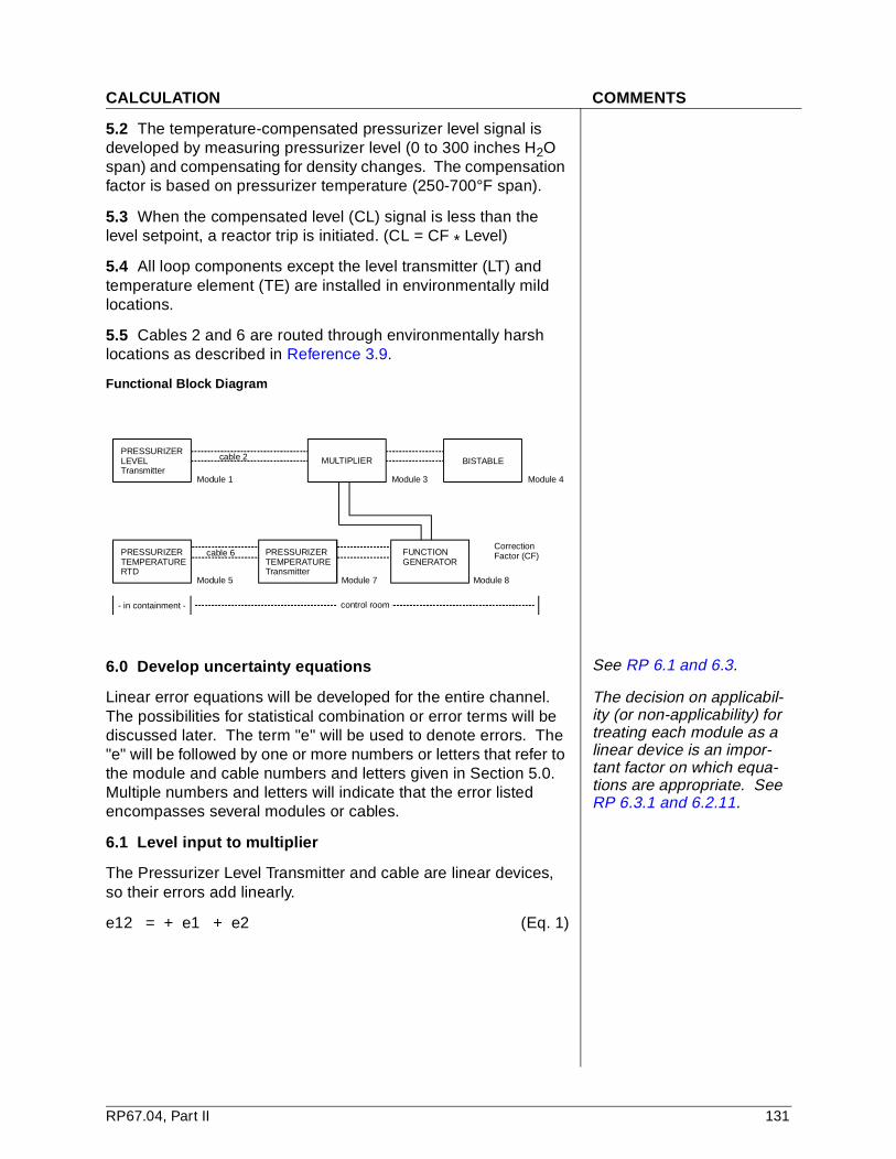
CALCULATION COMMENTS

5.2 The temperature-compensated pressurizer level signal is developed by measuring pressurizer level (0 to 300 inches H2O span) and compensating for density changes. The compensation factor is based on pressurizer temperature (250-700°F span).

5.3 When the compensated level (CL) signal is less than the level setpoint, a reactor trip is initiated. (CL = CF * Level)

5.4 All loop components except the level transmitter (LT) and temperature element (TE) are installed in environmentally mild locations.

5.5 Cables 2 and 6 are routed through environmentally harsh locations as described in Reference 3.9.

Functional Block Diagram

6.0 Develop uncertainty equations See RP 6.1 and 6.3.

Linear error equations will be developed for the entire channel. The possibilities for statistical combination or error terms will be discussed later. The term "e" will be used to denote errors. The "e" will be followed by one or more numbers or letters that refer to the module and cable numbers and letters given in Section 5.0. Multiple numbers and letters will indicate that the error listed encompasses several modules or cables.

The decision on applicabil-ity (or non-applicability) for treating each module as a linear device is an impor-tant factor on which equa-tions are appropriate. See RP 6.3.1 and 6.2.11.

6.1 Level input to multiplier

The Pressurizer Level Transmitter and cable are linear devices, so their errors add linearly.

e12 = + e1 + e2 (Eq. 1)

PRESSURIZERLEVELTransmitter

Module 1

cable 2

cable 6

Module 5 Module 7 Module 8

CorrectionFactor (CF)

Module 3 Module 4

PRESSURIZERTEMPERATURERTD

- in containment -

PRESSURIZERTEMPERATURETransmitter

FUNCTIONGENERATOR

MULTIPLIER BISTABLE

control room

RP67.04, Part II 131

CALCULATION COMMENTS

6.2 Pressurizer temperature input to function generator #1While temperature devices may not be "pure" linear devices, they are often suf-ficiently linear over the area of interest to allow the tem-perature devices to be treated as "linear."

The Pressurizer temperature RTD, cable, and Pressurizer temperature transmitter are linear devices, so their errors add linearly

e567 = + e5 + e6 + e7 (Eq. 2)

6.3 Function generator #1 input to multiplier See RP 6.3.1, Table 1, and Appendix K.

Function Generator #1 is a non-linear device that converts temperature to a correction factor. This will effectively multiply the temperature error by the slope of the correction factor curve at the point of interest.

e5678 = + slope * (e567) + e8 (Eq. 3)

Per Section 4.5, the slope changes with actual temperature, so the error of the function generator output also changes with slope.

6.4 Multiplier output

The multiplier is a non-linear device. Per Reference 3.12, Table 6-1, the output error is

e1235678 = (LEVEL * e5678) + (CF * e12)

+ (e5678 * e12) + e3 (Eq. 4)

where LEVEL is the uncompensated level, and CF is the actual correction factor. Reference 3.12 also notes that the third term, consisting of the product of two very small numbers, is insignifi-cantly small and may be neglected. Therefore

See RP Appendix K (Eq. K-15, K-16).

e1235678 = (LEVEL * e5678) + (CF * e12) + e3 (Eq. 5)

6.5 Bistable output error

The analog portion of the bistable compares the multiplier output to a fixed setpoint.

e12345678 = + e1235678 * e4 (Eq. 6)

6.6 Channel uncertainty This is an alternative representation to RP Equa-tions 6.10 a & b.

The channel uncertainty, CU, is the bistable output error.

CU = e12345678 (Eq. 7)

132 RP67.04, Part II

CALCULATION COMMENTS

Combining terms from Sections 6.1 through 6.5 yields

CU = + LEVEL * [slope * (e5 + e6 + e7) + e8]

+ CF * (e1 + e2) + e3 + e4 (Eq. 8)

6.7 Statistical combination of channel uncertainties

Each of the error terms in Section 6.6 potentially consists of random and non-random (bias) parts. Random parts may be combined statistically to account for the low probability that all random errors will peak at the same time. Per Reference 3.12, a square-root-sum-of-the-squares, or SRSS, technique is appropriate.

The following convention will be used: random errors will be subscripted with an "R"; positive bias errors will be subscripted with a "P"; and negative bias errors will be subscripted with an "N".

Therefore

The multiplication of ran-dom and bias uncertainties in module 3 produces addi-tional compound random terms. Since these terms are the product of two small numbers, they them-selves are smaller and insignificant. Using this approximation allows prop-agating the random and bias uncertainties indepen-dently until final summation. See RP Appendix K and Equations K-27 and K-28.

e1R is the random part of the Pressurizer Level Transmitter error.

e1P is the positive bias part of the Pressurizer Level Transmitter error.

e1N is the negative bias part of the Pressurizer Level Transmitter error.

Using this convention, the random channel uncertainty becomes

CUR2 = + [LEVEL * slope * (e5R + e6R +e7R )]2

+ (LEVEL * e8R)2

+ [CF * (e1R + e2R)]2 + e3R2 +e4R

2 (Eq. 9)

Similarly, the positive bias channel uncertainty becomes This is an alternative representation to RP Equa-tions 6.10 a & b.

CUP = + LEVEL * slope * (e5P + e6P + e7P)

+ LEVEL * e8P

+ CF * (e1P + e2P) + e3P + e4P (Eq. 10)

And the negative bias channel uncertainty becomes

CUN = - LEVEL * slope * (e5N + e6N + e7N)

- LEVEL * e8N

- CF * (e1N + e2N - e3N - e4N) (Eq. 11)

RP67.04, Part II 133

CALCULATION COMMENTS

7.0 Determine uncertainty data See RP 6.2.

7.1 Module uncertainties

The following uncertainty components will be addressed:

PM = Process Measurement effects.

Note : PM applies to the primary element only.

RA = Module Reference Accuracy specified by the manufacturer.

DR = Drift of the module over a specific time period.

TE = Temperature effect for the module. Although the temperature effects occur due to a common cause, they are random in sign and magnitude and are therefore considered independent.

MTE = Measurement and Test Equipment effect. See 4.3.3.

MSLBE = Main Stream Line Break Effect.

Radiation effect will not be addressed per Assumption 2.1.

Seismic effect will not be addressed per 4.3.

Changes in static pressure do not affect any equipment in this channel and will not be addressed further.

The effects of changes in power supply voltages have been accounted for in module reference accuracy and will not be addressed separately.

There are no primary element effects since no separate primary elements are used in this channel.

Therefore, the module error equation to be used is

e = PM + RA + DR + TE + MTE + MSLBE (Eq. 12)

As discussed under the channel uncertainty, these terms may contain both random and bias parts. The random parts of these terms may be combined using an SRSS technique, while the bias parts must be combined in accordance with their sign. Using the same sign conventions as above, this results in the following three equations:

eR2 = + PM2 + RAR

2 + DRR2 + TER

2 + MTER2 + MSLBER

2

(Eq. 13)

eP = + PMP + RAP + DRP + TEP + MTEP + MSLBEP (Eq. 14)

eN = + PMN + RAN + DRN + TEN + MTEN + MSLBEN (Eq. 15)

134 RP67.04, Part II

CALCULATION COMMENTS

7.2 Pressurizer level transmitter - Module 1 This application requires treating the transmitter channel as a "direct-acting" signal. This may not always be appropriate; i.e., as many applications would require compensation for a "reverse-acting" signal.

PM = -0.15% span, +3.93% span Section 4.7RA = ±0.25% span Reference 3.4, 3.6 Reference Accuracy (RA)

value, in this application, includes a "Setting Tolerance."

DR = ±1.10% span Reference 3.10TE = ±0.30% span Reference 3.4, 3.6MTE = ±0.06% span Section 2.3MSLBE = +6.80% span Reference 3.4, 3.6

Therefore, the module errors are

e1R = [0.252 + 1.12 + 0.32 + 0.062]½

= ±1.17% span

e1P = +3.93 + 6.80

= +10.73% span

e1N = -0.15% span

7.3 Level transmitter to mult iplier cable - Module 2

PM = N/ARA = N/ADR = N/ATE = N/AMTE = N/AMSLBE = +0.98% span Reference 3.9 See RP 6.2.10 and

Appendix D.

Therefore, the module errors are

e2R = ±0.0% spane2P = ±0.98% spane2N = ±0.0% span

7.4 Multiplier - Module 3

PM = N/ARA = ±0.10% span Reference 3.6DR = ±0.30% span Reference 3.6TE = ±0.03% span Reference 3.6MTE = ±0.025% span Section 2.3MSLBE = N/A

RP67.04, Part II 135

CALCULATION COMMENTS

Therefore, the module errors are

e3R = ±[0.102 + 0.302 + 0.032 + 0.0252]½

= ±0.32% span

e3P = ±0.0% span

e3N = ±0.0% span

7.5 Bistable - Module 4

PM = N/ARA = ±0.15% span Reference 3.6DR = ±0.227% span Section 4.2TE = ±0.03% span Reference 3.6MTE = ±0.04% span Section 2.3MSLBE = N/A

Therefore, the module errors are

e4R = ±[0.152 + 0.2272 + 0.032 + 0.042]½

= ±0.28% span

e4P = +0.0% span

e4N = -0.0% span

7.6 Pressurizer temperature RTD - Module 5

PM = N/A Section 4.8RA = ±0.15% span Reference 3.8DR = ±0.75% span Reference 3.8TE = N/AMTE = ±0.04% span Section 2.3MSLBE = ±0.00% span Reference 3.8

Therefore, the module errors are

e5R = ±[0.152 + 0.752 + 0.042]½

= ±0.77% span

e5P = +0.0% span

e5N = -0.0% span

7.7 RTD to temperature transmitter cable - Module 6

PM = N/ARA = N/ADR = N/ATE = N/AMTE = N/AMSLBE = +0.08% span Reference 3.9

136 RP67.04, Part II

CALCULATION COMMENTS

Therefore, the module errors are

e6R = ±0.0% span

e6P = +0.08% span

e6N = -0.0% span

7.8 Pressurizer temperature transmitter - Module 7

PM = N/ARA = ±0.20% span Reference 3.6DR = ±0.35% span Reference 3.6TE = ±0.03% span Reference 3.6MTE = ±0.05% span Section 2.3MSLBE = N/A

Therefore, the module errors are

e7R = ±[0.202 + 0.352 + 0.032 +0.052]½

= ±0.41% span

e7P = +0.0% span

e7N = -0.0% span

7.9 Function generator - Module 8

PM = N/ARA = ±0.53% span Reference 3.6DR = ±0.05% span Reference 3.6TE = ±0.10% span Reference 3.6MTE = ±0.13% span Section 2.3MSLBE = N/A

Therefore, the module errors are

e8R = ±[0.532 + 0.052 + 0.102 + 0.132]½

= ±0.56% span

e8P = +0.0% span

e8N = -0.0% span

8.0 Calculate channel uncertainty See RP 6.3.

8.1 Random channel uncertainty

From 6.7 (Eq. 9), the random channel uncertainty is

CUR2 = + [LEVEL * slope * (e5R + e6R + e7R)]2

+ (LEVEL * e8R)2

+ [CF * (e1R + e2R)]2

+ e3R2

+ e4R2 (Eq. 9)

RP67.04, Part II 137

CALCULATION COMMENTS

Substituting in the values obtained in Section 7.0,

CUR2 = + [LEVEL * slope * (0.77 + 0.0 + 0.41)]2

+ (LEVEL * 0.56)2

+ [CF * (1.17 + 0.00)]2

+ 0.322

+ 0.282

CUR = ± [(1.18 * LEVEL * slope)2 = (0.56 * LEVEL)2

+ (1.17 * CF)2 + 0.18]½

The MSLB is an overcooling transient, causing a contraction of the RCS. This contraction causes Pressurizer level to decrease below its normal range, which then initiates a reactor trip. The channel error increases with increasing LEVEL. A LEVEL of 50% (150 inches) will be used to conservatively estimate the channel error, in that any required reactor trip will occur below 50% span.

The Correction Factor is 1.0 at normal conditions and decreases as Pressurizer temperature decreases. Channel error increases with CF, so use of a large CF is conservative. The MSLB is an overcooling transient, so CF will decrease during the transient. A CF of 1.0 will be used to conservatively estimate the channel error.

The channel error increases with increasing slope. Slope increases with increasing CF. The slope at CF = 1 will be used to conservatively estimate channel error. This slope is 0.324 per 100°F or 0.00324 per °F.

Note that the first term, 1.18 * LEVEL * slope, needs careful attention to units. The percent temperature span is ±1.18; the percent level span is 0.5; and slope is (°F)-1. The simplest way to resolve this is to convert ±1.18% temperature span into (0.0118 * 450) = ±5.31°F and then carry out the multiplication.

CUR = ± [(5.31 * 0.5 * 0.00324)2 + (0.56 * 0.5)2

+ (1.17 * 1.0)2 + 0.18]½

= ± [0.00862 + 0.282 + 1.172 + 0.18]½

= ± 1.28% span

8.2 Positive bias channel uncertainty

The positive bias channel uncertainty equation (Eq. 10) is

CUP = + LEVEL * slope * (e5P + e6P + e7P)

+ LEVEL * e8P

+ CF * (e1P + e2P) + e3P + e4P (Eq. 10)

138 RP67.04, Part II

CALCULATION COMMENTS

Inserting the values from Section 7.0 and using the same development as in 8.1, the positive bias channel uncertainty becomes

CUP = + 0.5 * 0.00324 * [0 + .08 * (450/100) + 0]

+ 0.5 * 0

+ 1.0 * (10.73 + 0.98) + 0 + 0

CUP = + 0.00058 + 11.71 = + 11.71% span

8.3 Negative bias channel uncertainty

The negative bias channel uncertainty equation (Eq. 11) is

CUN = - LEVEL * slope * (e5N+ e6N + e7N)

- LEVEL * e8N

- CF * (e1N + e2N) - e3N - e4N (Eq. 11)

Inserting the values from Section 7.0 and using the same development as in 8.1, the positive bias channel uncertainty becomes

CUN = - 0.5 * 0.00324 * (0 + 0 + 0)

- 0.5 * 0

- 1.0 * (0.15 + 0) - 0 - 0

CUN = - 0.15% span

8.4 Total channel uncertainty

Therefore, the total channel uncertainty under 15 minutes of MSLB conditions is

CU = +12.99% span, -1.43% span

9.0 Obtain the analytical limit See RP Section 7.0

From Reference 3.1, the MSLB accident analysis requires that a reactor trip be initiated before Pressurizer level drops below 75 inches.

10.0 Determine the setpoint See RP Section 7.0

The trip setpoint (TS) will be the analytical limit + the channel error + the margin.

The analytical limit is 75 inches.

The channel error applicable to low trip is +12.99% span, or 39 inches.

RP67.04, Part II 139

CALCULATION COMMENTS

The normal operating band of Pressurizer level varies with power level, being 120 inches at zero power and 180 inches at full power. The minimum trip setpoint is (75 + 39) = 114 inches. Although this provides adequate operating margin versus the nominal Pressurizer level at full power, no additional margin will be added due to the small operating margin at zero power.

TS = Analytical Limit + CU + margin (Eq. 16)

= 75 + 39 + 0 inches

= 114 inches

11.0 Allowable Value See RP 7.0 and Appendix I.

To compute the allowable value for the Pressurizer level trip setpoint, the channel error as a result of conditions present during the surveillance test must be determined.

11.1 Channel Allowable Value Equations

The channel error equations for determination of the allowable value (Eqs. 9, 10, and 11) are the same as those given for the determination of channel uncertainty. However, all bias terms in this calculation arose from MSLB conditions, so only the random channel uncertainty equation is needed to determine channel allowable value uncertainty.

CAVUR2 = + [LEVEL * slope * e5R + e6R + e7R )]2

+ (LEVEL * e8R )2

+ [CF * (e1R + e2R )]2

+ e3R2

+ e4R2 (Eq. 17)

11.2 Module Allowable Value Equations

The module error equations for determination of the allowable value are similar to those given for the determination of channel uncertainty (Eqs. 9, 10, and 11) but reflect those error components that would be present in non-MSLB conditions. Again, the only bias errors in this calculation arose from MSLB conditions, so only the random module error equation is needed to determine the module allowable value error. Using "av" to indicate a module allowable value error, the module error equation becomes

avR2 = + RAR

2 + DRR2 + TER

2 + MTER2 (Eq. 18)

140 RP67.04, Part II

CALCULATION COMMENTS

11.3 Channel Allowable Value Uncertainty

Using Eq. 18, the module allowable value errors are

av1 = e1R = ± 1.17% span

av2 = 0

av3 = e3R = ± 0.32% span

av4 = e4R = ± 0.28% span

av5 = e5R = ± 0.77% span

av6 = 0

av7 = e7R = ± 0.41% span

av8 = e8R = ± 0.56% span

Substituting these values into Equation 13 gives

CAVUR2 = + [LEVEL * slope * (0.77 + 0.0 + 0.41)]2

+ (LEVEL * 0.56)2

+ [CF * (1.17 + 0.0)]2

+ 0.322

+ 0.282

CAVUR = ± [(1.18 * LEVEL * slope)2 + (0.56 * LEVEL)2

+ (1.17 * CF)2 + 0.18]½

Calibration is performed once a refueling at zero power. Therefore, LEVEL is 120 inches; CF is 0.64; and slope is .03/100oF, or .0003/oF. Substituting

CAVUR = ± [(5.31 * .4 * 0.0003)2 + (0.56 * .4)2

+ (1.17 * 0.64)2 + 0.18]½

CAVUR = ± 0.89% span

11.4 Channel Allowable Value

Per Section 10.0, the nominal trip setpoint is 114 inches. The channel allowable value error is ± 0.89% span, or ± 2.7 inches. Therefore, the channel allowable value is

AV = TS - CAVU (Eq. 19) Consistent with RP 7.3, Method 3.

= 114 - 2.7 inches

= 111.3 inches

RP67.04, Part II 141

CALCULATION COMMENTS

12.0 Summary

The Pressurizer level reactor trip is required for 15 minutes into a MSLB. Under these conditions, the worst-case channel error is +39 inches, -4.3 inches.

To assure a reactor trip before actual level reaches 80 inches, the trip setpoint should be set at 114 inches.

When performing surveillance testing at zero power, the channel error is expected to be ±2.7 inches. The channel is operable if it trips at no less than 111.3 inches.

142 RP67.04, Part II

EXAMPLE CALCULATION - RADIATION TRIP

CALCULATION COMMENTS

1.0 Purpose NOTE: The following format is for illustrative purposes only. See RP Preface, Section 10, and Page 105.

The purpose of this calculation is to establish instrument setpoints for the Reactor Building Exhaust Plenum Monitors (RIS-410 A,B). The HIGH trip setpoint is established by the ODCM (Reference 3.5) and maintained by plant Technical Specifications (Reference 3.4).

This calculation determines instrument bistable settings for both LOW (INOPERATIVE) and HIGH (ISOLATION) trip setpoints based upon instrument errors, process measurement uncertainties, and analytic limits taken from Reference 3.5.

2.0 Assumptions RP 5.2 and 5.3 were reviewed to identify poten-tially applicable factors.

2.1 M&TE uncertainty is significantly less than the reference accuracies of the installed equipment. The accuracy of a 4½-digit digital voltmeter (typically ±0.03%) is much less than 0.1 times the reference accuracy of the ratemeter (±3.0%). Similarly, the accuracy of the frequency counter used to calibrate the ratemeter (±10 ppm time base accuracy) greatly exceeds the ratemeter accuracy. Thus, these terms make no significant contributions to total channel uncertainty and are not present in the uncertainty formulas. Also, since digital sources and meter are used exclusively, any calibration technique errors due to misreading of the instruments would have an imperceivable impact on this calculation.

See RP 6.2.6.

2.2 The setting adjustment potentiometers are precision, multiple turn devices with a rated resolution of ±0.1 % SPAN. For the reasons in 2.1 above, the adjustment device does not contribute significantly to the final setting.

2.3 Since equipment specifications are given in percent equivalent linear full scale (% ELFS), this will be used as the common unit. To convert between process units (cpm, logarithmic) and % ELFS, the following conversion is used:

See last paragraph of RP 6.3.3.

FACTOR = 10[(% ELFS)(6)] where 6 is the number of decades for this application, % ELFS is the reference accuracy of the linear scale.

RP67.04, Part II 143

CALCULATION COMMENTS

This transformation does not allow exact mapping of symmetric intervals. For example, a symmetric ±1% ELFS interval transforms to a factor of 1.15 (or 1 ÷ 1.15 = 0.87). For this application using relatively small values, the positive interval (+ 15%) is approximately equal to the negative interval (-13%). For conservatism, all non-symmetric intervals are expanded to include symmetric limits (i.e., +15% and -13% are expanded to ±15%.)

2.4 The radioactive half-life of the installed check source is long compared to the surveillance interval (1.5 years).

If the check source half-life were not long compared to the surveillance interval, the low (inoperative) trip setpoint may require adjustment (lowering) to maintain the separation between the alarm point and the average value of the check source. Alterna-tively, the check source can be replaced.

3.0 References

3.1 Piping & Instrument Drawing M240

3.2 Analog Loop Diagram E62.4

3.3 Technical Manual NQ406-3, Radiation Monitoring System

3.4 Nuclear Unit One (NUO) Technical Specification

3.5 NUO Off-Site Dose Calculation Manual (ODCM)

3.6 Nuclear Radiation Detection, W. J. Price, McGraw-Hill

3.7 ANSI N13.10-1974, Continuous Monitored Effluent Radioactivity Instrumentation

3.8 Reg. Guide 1.105, Instrument Setpoints for Safety-Related Systems

3.9 ISA-S67.04, Setpoints for Nuclear Safety-Related Instrumentation

3.10 Telephone Conversation 89-1-17, from A. C. Smith to J. Parry (Radiation Monitoring, Inc., dated March 3, 1989)

144 RP67.04, Part II

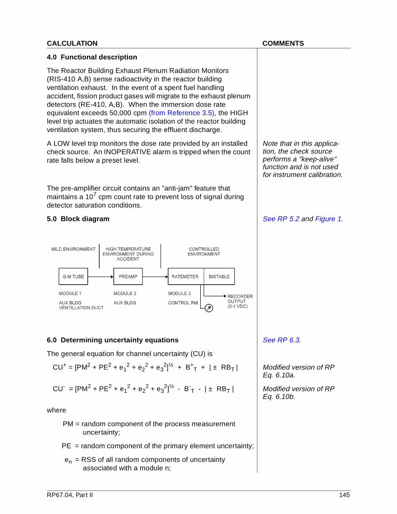
CALCULATION COMMENTS

4.0 Functional description

The Reactor Building Exhaust Plenum Radiation Monitors (RIS-410 A,B) sense radioactivity in the reactor building ventilation exhaust. In the event of a spent fuel handling accident, fission product gases will migrate to the exhaust plenum detectors (RE-410, A,B). When the immersion dose rate equivalent exceeds 50,000 cpm (from Reference 3.5), the HIGH level trip actuates the automatic isolation of the reactor building ventilation system, thus securing the effluent discharge.

A LOW level trip monitors the dose rate provided by an installed check source. An INOPERATIVE alarm is tripped when the count rate falls below a preset level.

Note that in this applica-tion, the check source performs a "keep-alive" function and is not used for instrument calibration.

The pre-amplifier circuit contains an "anti-jam" feature that maintains a 107 cpm count rate to prevent loss of signal during detector saturation conditions.

5.0 Block diagram See RP 5.2 and Figure 1.

6.0 Determining uncertainty equations See RP 6.3.

The general equation for channel uncertainty (CU) is

CU+ = [PM2 + PE2 + e12 + e2

2 + e32]½ + B+

T + | ± RBT | Modified version of RP Eq. 6.10a.

CU- = [PM2 + PE2 + e12 + e2

2 + e32]½ - B-

T - | ± RBT | Modified version of RP Eq. 6.10b.

where

PM = random component of the process measurement uncertainty;

PE = random component of the primary element uncertainty;

en = RSS of all random components of uncertainty associated with a module n;

RP67.04, Part II 145

CALCULATION COMMENTS

B+T = Algebraic sum of all bias estimates for all positive

biases in a channel;

B-T = Algebraic sum of all bias estimates for all negative

biases in a channel;

RBT = sum of the absolute value of all random bias (and arbitrary distribution) estimates in a channel.

The general equation for a module uncertainty is

e+ = + [RA2 + DR2 +TE2 +RE2 + SE2 +HE2 + SP2

+MTE2] ½ + B+ + | ± RB |

Modified version of RP Eq. 6.11a.

e- = - [RA2 + DR2 +TE2 +RE2 + SE2 +HE2 + SP2

+MTE2] ½ - B- - | ± RB |

Modified version of RP Eq. 6.11b.

where

e = module total uncertainty;

RA = module reference accuracy;

DR = module drift over a specified period;

TE = module temperature effect;

RE = module radiation effect;

SE = module seismic (vibration) effect;

HE = module humidity effect;

SP = module static pressure effect;

MTE = maintenance and test equipment used during module calibration;

B = bias uncertainty estimates associated with module;

RB = sum of absolute values of all random biases or abnormally distributed uncertainties for the module.

Note that this general form assumes that all uncertainties within the radical are random and approximately normally distributed.

7.0 Determine uncertainty data See RP 6.2.

The following discussion develops the uncertainty terms for each of the modules in the instrument channel. Any general equation terms that are not discussed are not relevant to this instrument channel.

According to the manufacturer, (Reference 3.10), the specified accuracies of the ratemeter and preamp modules include normal power supply variations, as well as normal environmental, temperature, and humidity effects.

146 RP67.04, Part II

CALCULATION COMMENTS

Static pressure effects do not apply to any modules in this calculation. Also, these instruments are not required to perform during or after a design-basis earthquake (DBE) or any other design-basis accident (DBA) that creates a hostile environment other than the accident described in Section 4.0.

7.1 Process measurement (PM) See RP 6.2.5.

For the LOW alarm setpoint (lowest decade), the integrating cir-cuit time constant is two seconds (Reference 3.3). For the HIGH alarm (trip) setpoint, a value of 0.02 seconds is given (Reference 3.3).

The random nature of the radioactive decay pro-cess causes a statistical uncertainty that depends upon the rate (cps) and the instrument time con-stant (RC). Analog rate-meters are typically designed for minimizing this uncertainty, yet must provide adequate response time.

For the 60 cpm check source (rtrue = 1 cps), the uncertainty is random and approximately normally distributed. The 95% probability limit is

2σ = ± (2r ÷ RC)½ Reference 3.6

where

r = signal count rate (cps);

RC = circuit time constant (sec).

For the LOW setpoint (1cps),

PMLOW = ± [2 (1) ÷ 2]½ = ±1 cps

(Error) Factor = (rtrue + rerror) ÷ rtrue = (1 + 1) ÷ 1 = 2.0

(100% relative error)

Converting to linear uncertainty units (see assumption 2.3),

2.0 = 106X; x = 5.0% ELFS

For the HIGH setpoint (50,000 cpm = 833 cps) from Reference 3.5,

PMHIGH = ± [2(833) ÷ 0.02 ]½ = ± 289 cps

Factor = (839 + 289) ÷ 839 = 1.35

1.35 = 106X; x = 2.2% ELFS

PMHIGH = ± 2.2% ELFS

RP67.04, Part II 147

CALCULATION COMMENTS

7.2 Primary element (PE)

There is no primary element. The Geiger-Muller (G-M) tube is treated as a sensor and designated as Module 1. The 2π geometry immersion dose to the sensors in the ventilation duct and the detector energy response are accounted for by the ODCM (Reference 3.5).

Note that this instrument setpoint calculation does not address the isotopic calibration of the sensors (G-M tubes). These effects are included in Reference 3.5.

7.3 G-M tube (Module 1)

For this application, the background noise is < 0.1 cps and has a negligible effect on the setpoint determination.

The G-M tube is basically an event counting device with an efficiency that is energy dependent and accounted for in the isoto-pic calibration process (detector efficiency calcu-lation). Thus, there is no reference accuracy asso-ciated with the tube. How-ever, there are unique effects to be considered. For low count rates, noise as well as background radiation may contribute significant bias errors.

Noise can be generated by operating the G-M tube at an elevated temperature. For this application, the operating temperature range in the ventilation duct is too low to cause any temperature effect (TE) bias.

The fill gas in the G-M tube is subject to long-term leakage, resulting in a gradual reduction in sensitivity (efficiency). This drift is very small and considered negligible over the 18-month-calibration interval (Reference 3.3).

For cases where back-ground represents a sig-nificant fraction of the indicated count rate, aver-age background values should be subtracted (as a constant correction) from the indicated count rate to obtain the process variable (true) count rate.

For the setpoint of 50,000 cpm (833 cps), the pulse, resolution effect is negligible. The formula for dead time correction is given in Reference 3.6, page 127 as

For very high count rates, there is a pulse resolution time associated with the G-M counter (and sys-tem). Typically, this effect becomes visible at > 105 cps and is caused by overlapping or near coincident pulses. It is a bias error, since indicated counts will always underestimate the true count rate.

148 RP67.04, Part II

CALCULATION COMMENTS

n = m ÷ (1 - mτ)

where n = true count rate (cps)

m = indicated count rate (cps)

τ = dead time (sec)

7.4 Pre-Amplifier (Module 2) See RP 6.2.2.

From the specification sheet in Reference 3.3, a temperature-noise effect of 100 cps for temperatures up to 150°F ambient to the pre-amp is used. As discussed earlier, noise addition is a positive bias (indicated value exceeds actual value).

The electronic pre-ampli-fier performs the neces-sary signal conditioning to drive the cable feed to the ratemeter. Although the output pulse height from the G-M tube is relatively large, the source imped-ance needs to be matched for the relatively long signal path to the ratemeter. The pre-amp is also a digital device that is capable of introducing electronic noise and con-tributing to pulse resolu-tion time.

TE = +100 cps (estimate limit of error)

This temperature effect is present only during accident (high temperature) conditions.

Converting to linear units,

FACTOR = (833 + 100) ÷ 833 = 1.12

1.12 = 106X; x = +0.8% ELFS

NOTE: This positive bias is an uncertainty estimate that may or may not be present. Although it is conservative for an increasing parameter (actual value < indicated value), accounting for the effect in this calculation assumes that the effect would always be present. If the effect was absent, its absence would result in a non-conservative condition (i.e., actual value > indicated value). Therefore, taking credit for this conservatism in this application is deemed imprudent. This term will not be included in the subsequent channel uncertainty equations.

7.5 Analog ratemeter (Module 3)

The analog ratemeter converts the 6 decades of input count rate into a linear output. It also includes electronic bistables that are set to trip at the desired values. Reference 3.3 gives the reference accuracy as ±3% ELFS (OUTPUT). Since the analog panel meter is small (3½ inches), the recorder output voltage is the output to which the ±3% ELFS applies. Significant additional uncertainties must be accounted for if analog panel meters are used (Reference 3.7).

See RP 6.2.6.4.

RP67.04, Part II 149

CALCULATION COMMENTS

The ratemeter converter stability (drift) is given in Reference 3.3 as ±0.5% ELFS for a 12-month period. Using the drift extension technique of linear extrapolation, one obtains

DR = ±0.75% ELFS for an 18-month interval.

This value will be treated as a random bias, since

1) The manufacturer does not have data to characterize a specific individual instrument (Reference 3.10); and

2) For simplicity, this single calculation applies to both instrumentation channels.

8.0 Calculate instrument channel uncertainty and trip setpoints

Since this is a calculation for a non-LSSS variable, RP Section 7.04 does not specifically apply.

Given the sources of module and process uncertainty developed in Section 7.0, the general equation of Section 6.0 is reduced to

HIGH SETPOINT:

CU = ± [PM2 + RA32]½ ± | ± RB3 |

= ± [ (2.2)2 + (3.0)2 ]½ ± | ±0.75 |

= ± 4.47% ELFS

From 2.3, FACTOR = 106(±0.0447) = (1.85)±1

SPHI = (AL) (FACTOR)

= (50,000 cpm) (1.85)-1 = 27,027 cpm (SET FOR TRIP ABOVE THIS VALUE)

LOW SETPOINT:

CU = ± [PM2 + RA32 ]½ ± | ± RB3 |

= ± [(5.0)2 + (3.0)2 ]½ ± | ±0.75 | = ±6.58% ELFS

Converting back to a Factor,

FACTOR = 106(±0.0658) = (2.48)±1

SPLO = (AL)(FACTOR)

= (60 cpm)(2.48)-1 = 24.2 cpm (SET FOR TRIP BELOW THIS VALUE)

In order to obtain accurate values the instrument bistable set-tings, the ratemeter setpoints will be set using the linear output (recorder) voltage. The transformation used is derived below.

150 RP67.04, Part II

CALCULATION COMMENTS

For the 6 decade analog ratemeter (K2 = 7, K1 = 1) with a 0 - 1 (A = 0, B = 1) VDC linear output, the values are summarized below.

POINT LOG VALUE LINEAR VALUE (CPM) (VOLTS)

LOWEST SCALE 10 0.000MARK

LOW TRIP 24.2 0.064

CHECK SOURCE 60 0.130

HIGH TRIP 27,027 0.572

HIGHEST 107 1.000SCALE MARK

Y 10

X K2 K1–( ) AK2– BK1+B A–

-------------------------------------------------------------------

10

6X 0– 1+1

--------------------------

10

6X 1+( )

= = =

X B A–( ) LOG Y+AK2 - BK1 K2 K1–

------------------------------------------------------------------------ LOG Y 0 1–+6

---------------------------------------= =

LOG Y 1–6

----------------------------=

RP67.04, Part II 151

CALCULATION COMMENTS

9.0 Determining the allowable value

Since the instruments are not contained in the LSSS Table in Reference 3.4, there are no Allowable Values.

10.0 Summary

The low bistable shall be set at 0.064 VDC using a digital voltmeter (DVM) connected to the recorder output. This value is significantly less than the 0.130 VDC check source average value and significantly greater than the 0.000 volt level at low scale. Similarly, the 0.572 VDC is significantly separated from the check source level and the high scale mark. Thus, the setpoint placements have a high probability of (1) tripping before reaching upper scale limits, and (2) avoiding false trips.

152 RP67.04, Part II

Developing and promulgating technically sound consensus standards,recommended practices, and technical reports is one of ISA's primarygoals. To achieve this goal the Standards and Practices Departmentrelies on the technical expertise and efforts of volunteer committeemembers, chairmen, and reviewers.

ISA is an American National Standards Institute (ANSI) accreditedorganization. ISA administers United States Technical Advisory Groups (USTAGs) and provides secretariat support for InternationalElectrotechnical Commission (IEC) and International Organization forStandardization (ISO) committees that develop process measurementand control standards. To obtain additional information on the Society's standards program, please write:

ISAAttn: Standards Department67 Alexander DriveP.O. Box 12277Research Triangle Park, NC 27709

ISBN: 1-55617-535-3