Download pdf - Mechanics of Composite Beams · 2018-09-25 · Mechanics of Composite Beams 529 ignored. So instead of 6X6 stiffness matrix for general laminate analysis we will have a 2X2 matrix

22

Mechanics of Composite Beams

Mehdi Hajianmaleki and Mohammad S. Qatu Mississippi State University

USA

1. Introduction

A structural element having one dimension many times greater than its other dimensions

can be a rod, a bar, a column, or a beam. The definition actually depends on the loading

conditions. A beam is a member mainly subjected to bending. The terms rod (or bar) and

column are for those members that are mainly subjected to axial tension and compression,

respectively.

Beams are one of the fundamental structural or machine components. Composite beams are

lightweight structures that can be found in many diverse applications including aerospace,

submarine, medical equipment, automotive and construction industries. Buildings, steel

framed structures and bridges are examples of beam applications in civil engineering. In

these applications, beams exist as structural elements or components supporting the whole

structure. In addition, the whole structure can be modeled at a preliminary level as a beam.

For example, a high rise building can be modeled as a cantilever beam, or a bridge modeled

as a simply supported beam. In mechanical engineering, rotating shafts carrying pulleys and

gears are examples of beams. In addition, frames in machines (e.g. a truck) are beams.

Robotic arms in manufacturing are modeled as beams as well. In aerospace engineering,

beams (curved and straight) are found in many areas of the plane or space vehicle. In

addition, the whole wing of a plane is often modeled as a beam for some preliminary

analysis. Innumerable other examples in these and other industries of beams exist.

This chapter is concerned with the development of the fundamental equations for the

mechanics of laminated composite beams. Two classes of theories are developed for

laminated beams. In the first class of theories, effects of shear deformation and rotary inertia

are neglected. This class of theories will be referred to as thin beam theories or classical

beam theories (CBT). This is typically accurate for thin beams and is less accurate for thicker

beams. In the second class of theories, shear deformation and rotary inertia effects are

considered. This class of theories will be referred to as thick beam theory or shear

deformation beam theory (SDBT).

This chapter can be mainly divided into two sections. First, static analysis where deflection and stress analysis for composite beams are performed and second dynamic analysis where natural frequencies of them are assessed. In many applications deflection of the beam plays a key role in the structure. For example, if an aircraft wig tip deflection becomes high, in addition to potential structural failure, it may deteriorate the wing aerodynamic performance. In this and other applications, beams can be subjected to dynamic loads. Imbalance in driveline shafts, combustion in crank shaft applications, wind on a bridge or a

www.intechopen.com

Advances in Composite Materials - Analysis of Natural and Man-Made Materials

528

structure, earthquake loading on a bridge or a structure, impact load when a vehicle goes over a pump are all examples of possible dynamic loadings that beam structures can be exposed to. All of these loads and others can excite the vibration of the beam structure. This can cause durability concerns or discomfort because of the resulting noise and vibration.

2. Stiffness of beams

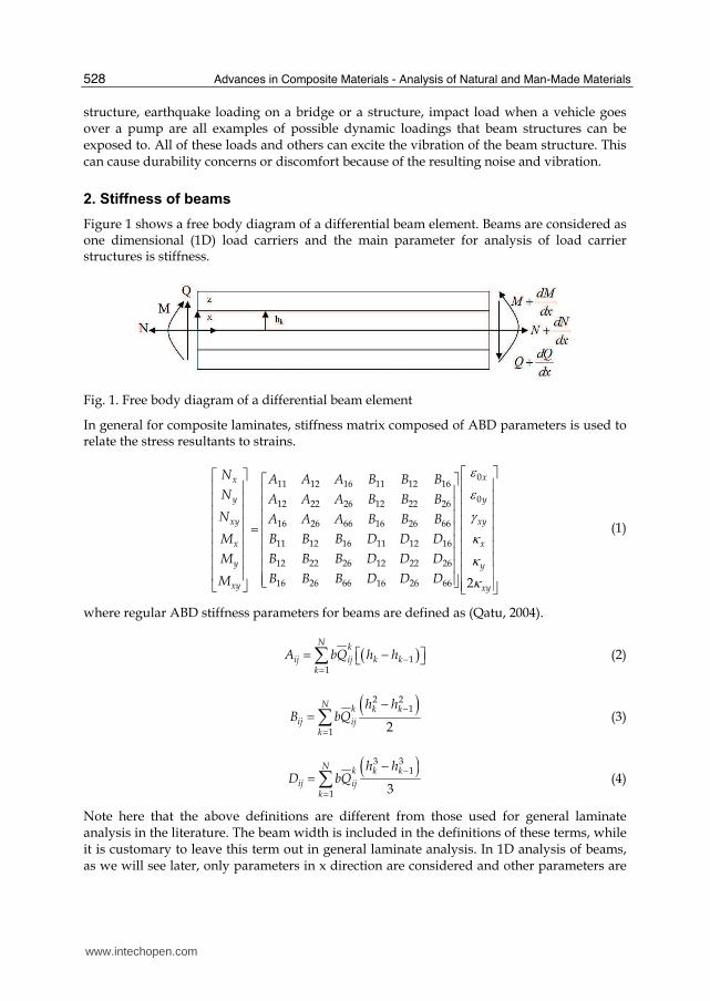
Figure 1 shows a free body diagram of a differential beam element. Beams are considered as one dimensional (1D) load carriers and the main parameter for analysis of load carrier structures is stiffness.

Fig. 1. Free body diagram of a differential beam element

In general for composite laminates, stiffness matrix composed of ABD parameters is used to relate the stress resultants to strains.

011 12 16 11 12 16

012 22 26 12 22 26

16 26 66 16 26 66

11 12 16 11 12 16

12 22 26 12 22 26

16 26 66 16 26 66 2

xx

y y

xy xy

x x

y y

xy xy

N A A A B B BN A A A B B B

N A A A B B B

M B B B D D D

M B B B D D D

B B B D D DM

εεγκκκ

⎡ ⎤⎡ ⎤ ⎡ ⎤ ⎢ ⎥⎢ ⎥ ⎢ ⎥ ⎢ ⎥⎢ ⎥ ⎢ ⎥ ⎢ ⎥⎢ ⎥ ⎢ ⎥ ⎢ ⎥⎢ ⎥ = ⎢ ⎥ ⎢ ⎥⎢ ⎥ ⎢ ⎥ ⎢ ⎥⎢ ⎥ ⎢ ⎥ ⎢ ⎥⎢ ⎥ ⎢ ⎥ ⎢⎢ ⎥ ⎢ ⎥⎣ ⎦ ⎢⎣ ⎦ ⎣ ⎦⎥⎥

(1)

where regular ABD stiffness parameters for beams are defined as (Qatu, 2004).

( )11

N k

ij k kijk

A bQ h h −=⎡ ⎤= −⎣ ⎦∑ (2)

( )2 2

1

1 2

N k k k

ij ijk

h hB bQ

−=

−=∑ (3)

( )3 3

1

1 3

N k k k

ij ijk

h hD bQ

−=

−=∑ (4)

Note here that the above definitions are different from those used for general laminate analysis in the literature. The beam width is included in the definitions of these terms, while it is customary to leave this term out in general laminate analysis. In 1D analysis of beams, as we will see later, only parameters in x direction are considered and other parameters are

www.intechopen.com


529

ignored. So instead of 6X6 stiffness matrix for general laminate analysis we will have a 2X2 matrix for CBT and 3X3 matrix for SDBT. This formulation has the disadvantage of not accounting for any coupling. To overcome this problem, we propose that instead of normal definition of A11, B11, and D11, one can use equivalent stiffness parameters that include couplings. That is why we will deal with stiffness parameters first.

2.1 Equivalent modulus

One approach for finding equivalent modulus for the whole laminate was proposed by

finding the inverse of the ABD matrix (J matrix) (Kaw, 2005). The laminate modulus of

elasticity is then defined as

1

44

[ ]b

E J ABDI J

−= = (5)

where J44 is the term in 4th row and 4th column of the inverse of the ABD matrix of the

laminate and I is the moment of inertia. If one wants to use this approach for finding

parameters A11, B11, and D11 the following formulas derived by authors should be used.

1111

bA

J= (6)

1114

1B

J= (7)

1144

bD

J= (8)

2.2 Equivalent stiffness parameters by Rios and Chan

Another approach using compliance matrix can be done by the following formulation (Rios

and Chan, 2010).

11 211

1111

1A

ba

d

=−

(9)

1111 11

1111

1B

a db

b

=−

(10)

11 211

1111

1D

bd

a

=−

(11)

where a11, b11, and d11 are relevant compliance matrix terms. Similar to previous section we

have a11=J11, b11=J14, d11=J44.

www.intechopen.com


530

2.3 Equivalent stiffness parameters by Vinson and Sierakowski Finding equivalent modulus of elasticity of each lamina and using normal definition of ABDs leads to the following formulation (Vinson and Sierakowski, 2002).

( ) ( ) ( ) ( )4 42 212

11 12 11 22

cos sin1 1 2cos sink k

k kkx E G E EE

θ θυ θ θ⎛ ⎞= + − +⎜ ⎟⎝ ⎠ (12)

Equivalent A11, B11 and D11 using these formulas would be

( )11 11

Nkx k k

k

A bE h h −== −∑ (13)

( )2 2

1

111 2

Nk kk

xk

h hB bE

−=

−=∑ (14)

( )3 3

1

111 3

Nk kk

xk

h hD bE

−=

−=∑ (15)

3. Static analysis

In static analysis section we will consider composite beams loaded with classical loading condition and derive differential equations for displacements. Those equations would be solved with classical boundary conditions of both ends simply supported and both ends clamped. We will use the static analyses to find deflection and stress of composite beams under both CBT and SDBT.

3.1 Classical beam theory

Applying the traditional assumptions for thin beams (normals to the beam midsurface remain straight and normal, both rotary inertia and shear deformation are neglected), strains and curvature change at the middle surface are: (Qatu, 1993, 2004)

00

u

xε ∂= ∂ ,

2

2

w

xκ ∂= − ∂ (16)

where u, w are displacements in x and z directions, respectively. Normal strain at any point would be

0 zε ε κ= + (17)

Force and moment resultants are calculated using

11 11 0

11 11

N A B

M B D

εκ

⎡ ⎤ ⎡ ⎤ ⎡ ⎤=⎢ ⎥ ⎢ ⎥ ⎢ ⎥⎣ ⎦ ⎣ ⎦ ⎣ ⎦ (18)

The equations of motion are

2

2 z

Mp

x

∂ = −∂ (19)

www.intechopen.com


531

x

Np

x

∂ = −∂ (20)

where px and pz are external forces per unit length in x and z direction, respectively. The potential strain energy stored in a beam during elastic deformation is

( )00

1 1

2 2

l

VPE dV N M dxσε ε κ= = +∫ ∫ (21)

writing this expression for every lamina and summing for all laminate we have

( )( )2 211 0 11 0 110

12

2

lPE A B D dxε ε κ κ= + +∫ (22)

substituting kinematic relations to equation (22) it will become

22 2 20 0

11 11 112 20

12

2

l u u w wPE A B D dx

x x x x

⎛ ⎞⎛ ⎞ ⎛ ⎞∂ ∂ ∂ ∂⎛ ⎞ ⎛ ⎞⎜ ⎟= + − + −⎜ ⎟ ⎜ ⎟⎜ ⎟ ⎜ ⎟⎜ ⎟ ⎜ ⎟⎜ ⎟∂ ∂ ∂ ∂⎝ ⎠ ⎝ ⎠⎝ ⎠ ⎝ ⎠⎝ ⎠∫ (23)

The work done by external forces on beam would be

( )00

1

2

l

x zW p u p w dx= +∫ (24)

The kinetic energy for each lamina is

( )1

2 20

0

1

2

k

k

l zk

z

u wKE b dx

t tρ

−

⎛ ⎞∂ ∂⎛ ⎞ ⎛ ⎞⎜ ⎟= + ⎜ ⎟⎜ ⎟⎜ ⎟∂ ∂⎝ ⎠⎝ ⎠⎝ ⎠∫ ∫ (25)

where ( )kρ is the lamina density per unit volume, and t is time. The kinetic energy of the entire beam is

2 2

01

02

l uI wKE dx

t t

⎛ ⎞∂ ∂⎛ ⎞ ⎛ ⎞⎜ ⎟= + ⎜ ⎟⎜ ⎟⎜ ⎟∂ ∂⎝ ⎠⎝ ⎠⎝ ⎠∫ (26)

where I1 is the average mass density of the beam per unit length. These energy expressions can be used in an energy-based analysis such as finite element or Ritz analyses.

3.1.1 Euler approach Inserting displacement relations in equations of motion will result in (Vinson and Sierakowski, 2002)

2 3

11 112 3( ) 0x

u wA B p x

x x

∂ ∂− + =∂ ∂ (27)

3 4

11 113 4( ) 0z

u wB D p x

x x

∂ ∂− + =∂ ∂ (28)

Solving these two equations for u and w will result in the following differential equations.

www.intechopen.com


532

2 4

11 11 11 114

11 11

( )( ) x

z

p xA D B w Bp x

A A xx

⎡ ⎤ ∂− ∂ = −⎢ ⎥ ∂∂⎢ ⎥⎣ ⎦ (29)

32

011 11 11 113

11 11

( )( ) x

z

p xuA D B Dp x

B B xx

⎡ ⎤ ∂∂− = −⎢ ⎥ ∂∂⎢ ⎥⎣ ⎦ (30)

Stress in the axial direction in any lamina can be found by the following equation

( ) 20

11 0 11 2x

u wQ z Q z

x xσ ε κ ⎛ ⎞∂ ∂= + = −⎜ ⎟⎜ ⎟∂ ∂⎝ ⎠ (31)

Different loading and boundary conditions can be applied to these equations in order to find equations for u and w. These boundary conditions are

Simply supported: 0, 0w M= =

Clamped: 0, 0dw

wdx

= =

Free: 0, 0V M= = where V and M are shear force and bending moment and are linearly dependent on third and second derivative of w respectively. Here, we propose solution for both ends simply supported and both ends clamped with constant loading q0. The reader is urged to apply other boundary conditions and find the equations for deflection. For specific case of simply supported boundary conditions at both ends and assuming u0(0)=0 we have

4 342

011 11 11

11

( ) 224

q lA D B x x xw x

A l l l

⎡ ⎤⎡ ⎤− ⎛ ⎞ ⎛ ⎞ ⎛ ⎞= − +⎢ ⎥⎢ ⎥ ⎜ ⎟ ⎜ ⎟ ⎜ ⎟⎝ ⎠ ⎝ ⎠ ⎝ ⎠⎢ ⎥ ⎢ ⎥⎣ ⎦ ⎣ ⎦ (32)

3 232

011 11 110

11

( ) 4 624

q lA D B x xu x

B l l

⎡ ⎤⎡ ⎤− ⎛ ⎞ ⎛ ⎞= −⎢ ⎥⎢ ⎥ ⎜ ⎟ ⎜ ⎟⎝ ⎠ ⎝ ⎠⎢ ⎥ ⎢ ⎥⎣ ⎦ ⎣ ⎦ (33)

( ) ( )220

11 11 11211 11 112

x

q l x xQ B zA

l lA D Bσ ⎡ ⎤⎛ ⎞ ⎛ ⎞= − −⎢ ⎥⎜ ⎟ ⎜ ⎟⎝ ⎠ ⎝ ⎠− ⎢ ⎥⎣ ⎦ (34)

( ) ( )011 11 112

11 11 11

12 1

2

z zxxz h h

q l xdz Q B zA dz

b x lb A D B

στ ∂ ⎡ ⎤⎛ ⎞= = − −⎜ ⎟⎢ ⎥∂ ⎝ ⎠− ⎣ ⎦∫ ∫ (35)

For clamped boundary conditions at both ends we have

4 3 242

011 11 11

11

( ) 224

q lA D B x x xw x

A l l l

⎡ ⎤⎡ ⎤− ⎛ ⎞ ⎛ ⎞ ⎛ ⎞= − +⎢ ⎥⎢ ⎥ ⎜ ⎟ ⎜ ⎟ ⎜ ⎟⎝ ⎠ ⎝ ⎠ ⎝ ⎠⎢ ⎥ ⎢ ⎥⎣ ⎦ ⎣ ⎦ (36)

3 232

011 11 110

11

( ) 4 6 224

q lA D B x x xu x

B l l l

⎡ ⎤⎡ ⎤− ⎛ ⎞ ⎛ ⎞ ⎛ ⎞= − +⎢ ⎥⎢ ⎥ ⎜ ⎟ ⎜ ⎟ ⎜ ⎟⎝ ⎠ ⎝ ⎠ ⎝ ⎠⎢ ⎥ ⎢ ⎥⎣ ⎦ ⎣ ⎦ (37)

www.intechopen.com


533

( ) ( )220

11 11 11211 11 11

1

62x

q l x xQ B zA

l lA D Bσ ⎡ ⎤⎛ ⎞ ⎛ ⎞= − + −⎢ ⎥⎜ ⎟ ⎜ ⎟⎝ ⎠ ⎝ ⎠− ⎢ ⎥⎣ ⎦

(38)

( ) ( )011 11 112

11 11 11

12 1

2

z zxxz h h

q l xdz Q B zA dz

b x lb A D B

στ ∂ ⎡ ⎤⎛ ⎞= = − −⎜ ⎟⎢ ⎥∂ ⎝ ⎠− ⎣ ⎦∫ ∫ (39)

One should note that for simply supported boundary condition the maximum moment and consequently maximum stress occurs at middle of the beam, while for the clamped case maximum stress occurs at two ends.

3.1.2 Matrix approach

Inserting the strain and curvature relations in the force and moment resultants equations and using those in the equations of motion, one can express the equations of motion in terms of displacements. Expressing those equations in matrix form we have

11 12 0

21 22 0

0

0x

z

L L u p

L L w p

⎡ ⎤ ⎡ ⎤ ⎡ ⎤ ⎡ ⎤+ =⎢ ⎥ ⎢ ⎥ ⎢ ⎥ ⎢ ⎥−⎣ ⎦ ⎣ ⎦ ⎣ ⎦ ⎣ ⎦ (40)

where 2

11 11 2L A

x

∂= ∂ , 4

22 11 4L D

x

∂= ∂ , 3

12 21 11 3L L B

x

∂= = − ∂ .

The beam is supposed to have simply supported boundary condition. So we have on x=0, a.

0 0x xw N M= = = (41)

The above equations of motion as well boundary terms are satisfied if one chooses displacements functions as

[ ] [ ]1

, cos( ), sin( )M

m m m mm

u w A x C xα α=

= ∑ (42)

where /m m aα π= and a is the beam length. The external forces can be expanded in a Fourier series in x

[ ] ( ) ( )1

, sin , cosM

x z xm m zm mm

p p p x p xα α=⎡ ⎤= ⎣ ⎦∑ (43)

Substituting these equations in the equations of motion we have the characteristic equation

11 12

21 22

0m xm

m zm

C C A p

C C C p

⎡ ⎤ ⎡ ⎤ ⎡ ⎤+ =⎢ ⎥ ⎢ ⎥ ⎢ ⎥−⎣ ⎦ ⎣ ⎦ ⎣ ⎦ (44)

111 12

21 22

m xm

m zm

A C C p

C C C p

− −⎡ ⎤ ⎡ ⎤ ⎡ ⎤=⎢ ⎥ ⎢ ⎥ ⎢ ⎥⎣ ⎦ ⎣ ⎦ ⎣ ⎦ (45)

where 211 11mC Aα= − , 4

22 11mC Dα= , 321 12 11mC C Bα= − = . Stress in the axial direction would be

found using the following procedure.

www.intechopen.com


534

10 11 11

11 11

A B N

B D M

εκ

−⎡ ⎤ ⎡ ⎤ ⎡ ⎤=⎢ ⎥ ⎢ ⎥ ⎢ ⎥⎣ ⎦ ⎣ ⎦ ⎣ ⎦ (46)

( )11 0x Q zσ ε κ= + (47)

3.2 Shear deformation beam theory

The inclusion of shear deformation in the analysis of beams was first made in early years of twentieth century (Timoshenko, 1921). A lot of models have been proposed based on this theory since then. In this chapter a first order shear deformation theory (FSDT) approach is presented to account for shear deformation and rotary inertia (Qatu, 1993, 2004).

0 0,u u z w wψ= + = (48)

Strains and curvature changes at the middle surface are:

00

u

xε ∂= ∂ ,

x

ψκ ∂= ∂ , w

xγ ψ∂= +∂ (49)

where 0ε is middle surface strain, γ is the shear strain at the neutral axis and ψ is the rotation of a line element perpendicular to the original direction. Normal strain at any point can be found using equation 17. Force and moment resultants as well as shear forces are calculated using

11 11 0

11 11

55

0

0

0 0

N A B

M B D

Q A

εκγ

⎡ ⎤ ⎡ ⎤ ⎡ ⎤⎢ ⎥ ⎢ ⎥ ⎢ ⎥=⎢ ⎥ ⎢ ⎥ ⎢ ⎥⎢ ⎥ ⎢ ⎥ ⎢ ⎥⎣ ⎦ ⎣ ⎦ ⎣ ⎦ (50)

where for A55 we have (Vinson and Sierakowski, 2002).

( ) ( )3 355 1 12

1 55

5 4

4 3

kN

k k k kk

A bQ h h h hh

− −=⎡ ⎤= − − −⎢ ⎥⎣ ⎦∑ (51)

The equations of motion considering rotary inertia and shear deformation would be

x

Np

x

∂ = −∂ (52)

z

Qp

x

∂ =∂ (53)

0M

Qx

∂ − =∂ (54)

The potential strain energy stored in a beam during elastic deformation is

00

1 1

2 2

l

VPE dV N M Q dx

x

ψσε ε γ∂⎛ ⎞= = + +⎜ ⎟∂⎝ ⎠∫ ∫ (55)

www.intechopen.com


535

Writing this expression for every lamina and summing for all laminate we have (Vinson and Sierakowski, 2002)

( )( )2 2 211 0 11 0 11 550

12

2

lPE A B D A dxε ε κ κ γ= + + +∫ (56)

substituting kinematic relations to equation (56) it will become

2 2 2

0 011 11 11 550

12

2

l u u wPE A B D A dx

x x x x x

ψ ψ ψ⎛ ⎞∂ ∂ ∂ ∂ ∂⎛ ⎞ ⎛ ⎞⎛ ⎞ ⎛ ⎞ ⎛ ⎞⎜ ⎟= + + + +⎜ ⎟ ⎜ ⎟ ⎜ ⎟⎜ ⎟ ⎜ ⎟⎜ ⎟∂ ∂ ∂ ∂ ∂⎝ ⎠ ⎝ ⎠ ⎝ ⎠⎝ ⎠ ⎝ ⎠⎝ ⎠∫ (57)

The work done by external forces on beam is found by equation (24). Finding the kinetic energy for each layer and then summing for all layers yield the kinetic energy of the entire beam.

2 2 2

0 01 1 2 30

2l u uw

KE I I I I dxt t t t t

ψ ψ⎛ ⎞∂ ∂∂ ∂ ∂⎛ ⎞ ⎛ ⎞⎛ ⎞ ⎛ ⎞ ⎛ ⎞⎜ ⎟= + + +⎜ ⎟ ⎜ ⎟ ⎜ ⎟⎜ ⎟ ⎜ ⎟⎜ ⎟∂ ∂ ∂ ∂ ∂⎝ ⎠ ⎝ ⎠ ⎝ ⎠⎝ ⎠ ⎝ ⎠⎝ ⎠∫ (58)

These energy expressions can be used in an energy-based analysis such as finite element or Ritz analyses.

3.2.1 Euler approach

Inserting displacement relations in equations of motion will result in

2 2

011 112 2

( ) 0x

uA B p x

x x

ψ∂ ∂+ + =∂ ∂ (59)

( )2

55 20z

wA p x

x x

ψ⎛ ⎞∂ ∂+ + =⎜ ⎟⎜ ⎟∂ ∂⎝ ⎠ (60)

2 2

11 11 552 20

u dwB D A

dxx x

ψ ψ∂ ∂ ⎛ ⎞+ − + =⎜ ⎟∂ ∂ ⎝ ⎠ (61)

Taking second derivative of equation (60) and solving for 3

3x

ψ∂∂ from equations (59, 61) will

result in following equations.

24

11 114 2 2 2

5511 11 11 11 11 11

( ) ( )1( ) z x

z

p x p xw A Bp x

A xx A D B x A D B

⎡ ⎤⎡ ⎤ ⎡ ⎤∂ ∂∂ = − −⎢ ⎥⎢ ⎥ ⎢ ⎥ ∂∂ − ∂ −⎢ ⎥ ⎢ ⎥⎢ ⎥⎣ ⎦ ⎣ ⎦⎣ ⎦ (62)

3

0 113 2

1111 11 11

( )1( ) x

z

p xu Bp x

A xx A D B

⎡ ⎤ ∂∂ = −⎢ ⎥ ∂∂ −⎢ ⎥⎣ ⎦ (63)

3

11 113 2 2

11 11 11 11 11 11

( )( )x

z

p xB Ap x

xx A D B A D B

ψ ⎡ ⎤ ⎡ ⎤∂∂ = −⎢ ⎥ ⎢ ⎥∂∂ − −⎢ ⎥ ⎢ ⎥⎣ ⎦ ⎣ ⎦ (64)

www.intechopen.com


536

For specific case of pz(x)=q0 with simply supported boundary conditions we have

4 3 24 2

0 0112

5511 11 11

( ) 224 2

q l q lA x x x x xw x

l l l A l lA D B

⎡ ⎤ ⎡ ⎤⎛ ⎞ ⎛ ⎞ ⎛ ⎞ ⎛ ⎞ ⎛ ⎞ ⎛ ⎞= − + + +⎢ ⎥ ⎢ ⎥⎜ ⎟ ⎜ ⎟ ⎜ ⎟ ⎜ ⎟ ⎜ ⎟ ⎜ ⎟⎜ ⎟− ⎝ ⎠ ⎝ ⎠ ⎝ ⎠ ⎝ ⎠ ⎝ ⎠⎢ ⎥ ⎢ ⎥⎝ ⎠ ⎣ ⎦ ⎣ ⎦ (65)

3 23

0 0112

5511 11 11

( ) 1 4 624 2

q l q lA x xx

l l AA D Bψ ⎡ ⎤⎛ ⎞ ⎛ ⎞ ⎛ ⎞= − + +⎢ ⎥⎜ ⎟ ⎜ ⎟ ⎜ ⎟⎜ ⎟− ⎝ ⎠ ⎝ ⎠⎢ ⎥⎝ ⎠ ⎣ ⎦

(66)

( ) ( )22 20 0

11 11 1125511 11 11

2

2x

q l q l zx xQ B zA

l l AA D Bσ ⎡ ⎤⎛ ⎞ ⎛ ⎞= − − −⎢ ⎥⎜ ⎟ ⎜ ⎟⎝ ⎠ ⎝ ⎠− ⎢ ⎥⎣ ⎦

(67)

maximum deflection would occur at middle of the beam and it would be

4 2

0 011max 2

5511 11 11

5

384 8

q l q lAw

AA D B

⎛ ⎞= +⎜ ⎟⎜ ⎟−⎝ ⎠ (68)

The first term in equation (68) is deflection due to bending and the second term is due to shear. For clamped boundary condition one can use the term due to bending from CBT analysis and add the term due to shear.

3.2.2 Matrix approach

Expressing equations of motion in terms of displacement we have in matrix form

11 12 13 0

21 22 23 0

31 32 33

0

0

0 0

x

z

L L L u p

L L L w p

L L L ψ⎡ ⎤ ⎡ ⎤ ⎡ ⎤ ⎡ ⎤⎢ ⎥ ⎢ ⎥ ⎢ ⎥ ⎢ ⎥+ − =⎢ ⎥ ⎢ ⎥ ⎢ ⎥ ⎢ ⎥⎢ ⎥ ⎢ ⎥ ⎢ ⎥ ⎢ ⎥⎣ ⎦ ⎣ ⎦ ⎣ ⎦ ⎣ ⎦

(69)

where2 2 2 2

11 11 22 55 33 11 55 13 31 112 2 2 2, , , L A L A L D A L L B

x x x x

∂ ∂ ∂ ∂= = − = − = =∂ ∂ ∂ ∂ ,

23 32 55 12 21, 0L L A L Lx

∂= = − = =∂ . The following simply supported boundary conditions are

used on x=0, a

0 0xw N

x

ψ∂= = =∂ (70)

The above equations would be satisfied if

[ ] [ ]0 01

, , cos( ), sin( ), cos( )m

m m m m m mm

u w A x C x B xψ α α α=

= ∑ (71)


111 12 13

12 22 23

13 23 33 0

m xm

m zm

m

A C C C p

C C C C p

B C C C

− −⎡ ⎤ ⎡ ⎤ ⎡ ⎤⎢ ⎥ ⎢ ⎥ ⎢ ⎥=⎢ ⎥ ⎢ ⎥ ⎢ ⎥⎢ ⎥ ⎢ ⎥ ⎢ ⎥⎣ ⎦ ⎣ ⎦ ⎣ ⎦ (72)

www.intechopen.com


537

where 211 11mC Aα= − , 2

22 55mC Aα= , 233 11 55mC D Aα= − − , 2

31 13 11mC C Bα= = − ,

23 32 55 mC C A α= − = , 21 12 0C C= = .

4. Dynamic analysis

To the knowledge of authors, there is no simple approach for dynamic analysis of composite beams considering all kinds of couplings. A review was conducted on advances in analysis of laminated beams and plates vibration and wave propagation (Kapania and Raciti, 1989. Another review was done on the published literature of vibrations of curved bars, beams, rings and arches of arbitrary shape which lie in a plane (Chidamparam and Leissa, 1993). Among FSDT works, some were validated for symmetric cross-ply laminates that have no coupling (Chandrashekhara et al., 1990; Krishnaswamy et al., 1992; Abramovich et al., 1994). In some other models, symmetric beams having fibers in one direction (only bending-twisting coupling) were considered (Teboub and Hajela, 1995; Banerjee 1995, 2001; Lee at al., 2004). Some FSDT models were validated for cross-ply laminates that have only bending-stretching coupling (Eisenberger et al. 1995; Qatu 1993, 2004). Higher order shear deformation theories (HSDT) were also developed for composite beams to address issues of cross sectional warping and transverse normal strains. Some were validated for cross-ply laminates (Khdier and Reddy, 1997; Kant et al., 1998; Matsunaga, 2001; Subramanian, 2006). Other theories like zigzag theory (Kapuria et al. 2004) were used to satisfy continuity of transverse shear stress through the laminate and showed to be accurate for natural frequency calculations of beams with specific geometry and lay-up (symmetric or cross-ply laminates). Another theory was global-local higher order theory (Zhen and Wanji, 2008) that was validated for cross-ply laminates. In this section, classic and FSDT beam models will be evaluated for their accuracy in a vibration analysis using different approaches for stiffness parameters calculation. Their results will be compared with those obtained using a 3D finite element model for different laminates (unidirectional, symmetric and asymmetric cross ply and symmetric and asymmetric angle-ply). The accurate model presented would then be verified for composite shafts.

4.1 Classical beam theory

Equations of motion for dynamic analysis of laminated beams would be

2 2

12 2 z

M wI p

x t

∂ ∂= −∂ ∂ (73)

2

1 2 x

N uI p

x t

∂ ∂= −∂ ∂ (74)

where ( )( )1 1

1

Nk

k kk

I b h hρ −== −∑ . Expressing those equations in matrix form we have for free

vibration

2

11 12 0 1 0

221 22 0 1 0

0 0

0 0

L L u I u

L L w I wt

−⎡ ⎤ ⎡ ⎤ ⎡ ⎤ ⎡ ⎤ ⎡ ⎤∂+ =⎢ ⎥ ⎢ ⎥ ⎢ ⎥ ⎢ ⎥ ⎢ ⎥∂⎣ ⎦ ⎣ ⎦ ⎣ ⎦ ⎣ ⎦ ⎣ ⎦ (75)

www.intechopen.com


538

The equations of motion as well as simply supported boundary terms are satisfied if one chooses displacements as

[ ] [ ]1

, cos( ), sin( ) sin( )M

m m m mm

u w A x C x tα α ω=

= ∑ (76)


11 12 12

21 22 1

00

0m m xm

m m zm

C C A I A p

C C C I C pω⎡ ⎤ ⎡ ⎤ ⎡ ⎤ ⎡ ⎤ ⎡ ⎤+ + =⎢ ⎥ ⎢ ⎥ ⎢ ⎥ ⎢ ⎥ ⎢ ⎥− −⎣ ⎦ ⎣ ⎦ ⎣ ⎦ ⎣ ⎦ ⎣ ⎦ (77)

The nontrivial solution for natural frequency can be found by setting the determinant of characteristic equation of matrix to zero. One should note here that if the laminate is symmetric, the B11 term vanishes and the bending frequencies are totally decoupled from axial ones. As a result, the following well-known formula for the natural frequencies of a symmetrically laminated simply supported composite beam can be applied:

2

11n

n D

A

πω ρ⎛ ⎞= ⎜ ⎟⎝ ⎠`

(78)

where ρ is density, ` is length and A is the cross section area of the beam. As we will see later it cannot be used for thick laminates and those that have any kind of coupling.

4.2 Shear deformation beam theory

The equations of motion considering rotary inertia and shear deformation would be (Qatu, 1993, 2004)

2 2

1 22 2 x

N uI I p

x t t

ψ∂ ∂ ∂= + −∂ ∂ ∂ (79)

2

1 2z

Q wp I

x t

∂ ∂− = −∂ ∂ (80)

2 2

2 32 2

M uQ I I

x t t

ψ∂ ∂ ∂− = +∂ ∂ ∂ (81)

where ( ) ( ) ( ) ( )( ) 2 2 3 31 2 3 1 1 1

1

1 1, , , ,

2 3

Nk

k k k k k kk

I I I b h h h h h hρ − − −=⎛ ⎞= − − −⎜ ⎟⎝ ⎠∑ . So by expressing

equations of motion in terms of displacement we have in matrix form (for free vibration)

11 12 13 0 1 2 02

21 22 23 0 1 02

31 32 33 2 3

0 0

0 0 0

0 0

L L L u I I u

L L L w I wt

L L L I Iψ ψ⎡ ⎤ ⎡ ⎤ ⎡ ⎤ ⎡ ⎤ ⎡ ⎤∂⎢ ⎥ ⎢ ⎥ ⎢ ⎥ ⎢ ⎥ ⎢ ⎥− − =⎢ ⎥ ⎢ ⎥ ⎢ ⎥ ⎢ ⎥ ⎢ ⎥∂⎢ ⎥ ⎢ ⎥ ⎢ ⎥ ⎢ ⎥ ⎢ ⎥⎣ ⎦ ⎣ ⎦ ⎣ ⎦ ⎣ ⎦ ⎣ ⎦

(82)

Equations of motion as long as simply supported boundary condition would be satisfied if

www.intechopen.com


539

[ ] [ ]0 01

, , cos( ), sin( ), cos( ) sin( )M

m m m m m mm

u w A x C x B x tψ α α α ω=

= ∑ (83)


11 12 13 1 2

212 22 23 1

13 23 33 2 3

0

0 0 0

0 0

m m xm

m m zm

m m

C C C A I I A p

C C C C I C p

C C C B I I B

ω⎡ ⎤ ⎡ ⎤ ⎡ ⎤ ⎡ ⎤ ⎡ ⎤⎢ ⎥ ⎢ ⎥ ⎢ ⎥ ⎢ ⎥ ⎢ ⎥+ − + − =⎢ ⎥ ⎢ ⎥ ⎢ ⎥ ⎢ ⎥ ⎢ ⎥⎢ ⎥ ⎢ ⎥ ⎢ ⎥ ⎢ ⎥ ⎢ ⎥⎣ ⎦ ⎣ ⎦ ⎣ ⎦ ⎣ ⎦ ⎣ ⎦

(84)

The nontrivial solution for natural frequency can be found by setting the determinant of characteristic equation matrix to zero.

5. Case studies

5.1 Rectangular beam

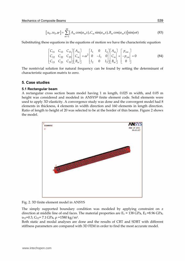
A rectangular cross section beam model having 1 m length, 0.025 m width, and 0.05 m height was considered and modeled in ANSYS® finite element code. Solid elements were used to apply 3D elasticity. A convergence study was done and the convergent model had 8 elements in thickness, 4 elements in width direction and 160 elements in length direction. Ratio of length to height of 20 was selected to be at the border of thin beams. Figure 2 shows the model.

Fig. 2. 3D finite element model in ANSYS

The simply supported boundary condition was modeled by applying constraint on z direction at middle line of end faces. The material properties are E1 = 138 GPa, E2 =8.96 GPa, υ12=0.3, G12= 7.1 GPa, ρ =1580 kg/m3. Both static and modal analyses are done and the results of CBT and SDBT with different stiffness parameters are compared with 3D FEM in order to find the most accurate model.

www.intechopen.com


540

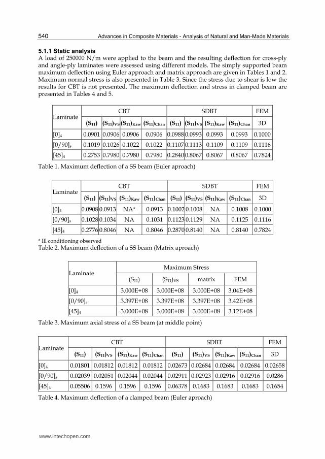
5.1.1 Static analysis A load of 250000 N/m were applied to the beam and the resulting deflection for cross-ply and angle-ply laminates were assessed using different models. The simply supported beam maximum deflection using Euler approach and matrix approach are given in Tables 1 and 2. Maximum normal stress is also presented in Table 3. Since the stress due to shear is low the results for CBT is not presented. The maximum deflection and stress in clamped beam are presented in Tables 4 and 5.

CBT SDBT FEM Laminate

(S11) (S11)VS (S11)Kaw (S11)Chan (S11) (S11)VS (S11)Kaw (S11)Chan 3D

[0]4 0.0901 0.0906 0.0906 0.0906 0.0988 0.0993 0.0993 0.0993 0.1000

[0/90]s 0.1019 0.1026 0.1022 0.1022 0.1107 0.1113 0.1109 0.1109 0.1116

[45]4 0.2753 0.7980 0.7980 0.7980 0.2840 0.8067 0.8067 0.8067 0.7824

Table 1. Maximum deflection of a SS beam (Euler aproach)



[0]4 0.0908 0.0913 NA* 0.0913 0.1002 0.1008 NA 0.1008 0.1000

[0/90]s 0.1028 0.1034 NA 0.1031 0.1123 0.1129 NA 0.1125 0.1116

[45]4 0.2776 0.8046 NA 0.8046 0.2870 0.8140 NA 0.8140 0.7824

* Ill conditioning observed Table 2. Maximum deflection of a SS beam (Matrix aproach)

Maximum Stress Laminate

(S11) (S11)VS matrix FEM

[0]4 3.000E+08 3.000E+08 3.000E+08 3.04E+08

[0/90]s 3.397E+08 3.397E+08 3.397E+08 3.42E+08

[45]4 3.000E+08 3.000E+08 3.000E+08 3.12E+08

Table 3. Maximum axial stress of a SS beam (at middle point)



[0]4 0.01801 0.01812 0.01812 0.01812 0.02673 0.02684 0.02684 0.02684 0.02658

[0/90]s 0.02039 0.02051 0.02044 0.02044 0.02911 0.02923 0.02916 0.02916 0.0286

[45]4 0.05506 0.1596 0.1596 0.1596 0.06378 0.1683 0.1683 0.1683 0.1654

Table 4. Maximum deflection of a clamped beam (Euler aproach)

www.intechopen.com


541

Maximum Stress Laminate

(S11) (S11)VS matrix FEM

[0]4 1.000E+08 1.00E+08 1.000E+08 1.00E+08

[0/90]s 1.132E+08 1.132E+08 1.132E+08 1.16E+08

[45]4 1.000E+08 1.00E+08 1.000E+08 1.00E+08

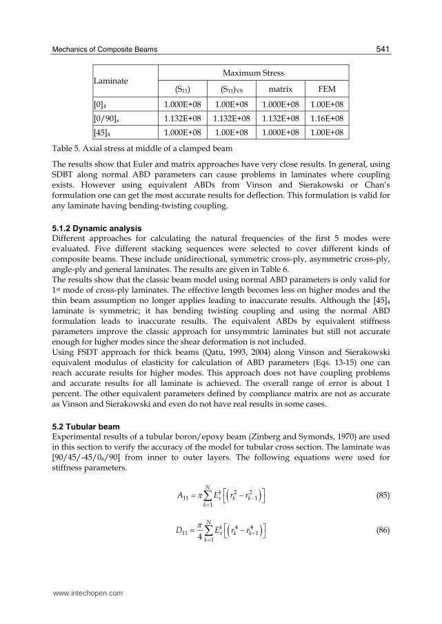
Table 5. Axial stress at middle of a clamped beam

The results show that Euler and matrix approaches have very close results. In general, using SDBT along normal ABD parameters can cause problems in laminates where coupling exists. However using equivalent ABDs from Vinson and Sierakowski or Chan’s formulation one can get the most accurate results for deflection. This formulation is valid for any laminate having bending-twisting coupling.

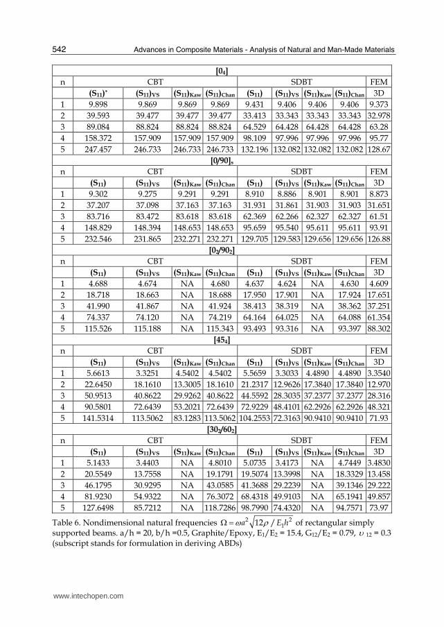
5.1.2 Dynamic analysis

Different approaches for calculating the natural frequencies of the first 5 modes were evaluated. Five different stacking sequences were selected to cover different kinds of composite beams. These include unidirectional, symmetric cross-ply, asymmetric cross-ply, angle-ply and general laminates. The results are given in Table 6. The results show that the classic beam model using normal ABD parameters is only valid for 1st mode of cross-ply laminates. The effective length becomes less on higher modes and the thin beam assumption no longer applies leading to inaccurate results. Although the [45]4 laminate is symmetric; it has bending twisting coupling and using the normal ABD formulation leads to inaccurate results. The equivalent ABDs by equivalent stiffness parameters improve the classic approach for unsymmtric laminates but still not accurate enough for higher modes since the shear deformation is not included. Using FSDT approach for thick beams (Qatu, 1993, 2004) along Vinson and Sierakowski equivalent modulus of elasticity for calculation of ABD parameters (Eqs. 13-15) one can reach accurate results for higher modes. This approach does not have coupling problems and accurate results for all laminate is achieved. The overall range of error is about 1 percent. The other equivalent parameters defined by compliance matrix are not as accurate as Vinson and Sierakowski and even do not have real results in some cases.

5.2 Tubular beam

Experimental results of a tubular boron/epoxy beam (Zinberg and Symonds, 1970) are used in this section to verify the accuracy of the model for tubular cross section. The laminate was [90/45/-45/06/90] from inner to outer layers. The following equations were used for stiffness parameters.

( )2 211 1

1

Nkx k k

k

A E r rπ −=⎡ ⎤= −⎣ ⎦∑ (85)

( )4 411 1

14

Nkx k k

k

D E r rπ

−=⎡ ⎤= −⎣ ⎦∑ (86)

www.intechopen.com


542

[04]

n CBT SDBT FEM

(S11)* (S11)VS (S11)Kaw (S11)Chan (S11) (S11)VS (S11)Kaw (S11)Chan 3D

1 9.898 9.869 9.869 9.869 9.431 9.406 9.406 9.406 9.373

2 39.593 39.477 39.477 39.477 33.413 33.343 33.343 33.343 32.978

3 89.084 88.824 88.824 88.824 64.529 64.428 64.428 64.428 63.28

4 158.372 157.909 157.909 157.909 98.109 97.996 97.996 97.996 95.77

5 247.457 246.733 246.733 246.733 132.196 132.082 132.082 132.082 128.67

[0/90]s

n CBT SDBT FEM


1 9.302 9.275 9.291 9.291 8.910 8.886 8.901 8.901 8.873

2 37.207 37.098 37.163 37.163 31.931 31.861 31.903 31.903 31.651

3 83.716 83.472 83.618 83.618 62.369 62.266 62.327 62.327 61.51

4 148.829 148.394 148.653 148.653 95.659 95.540 95.611 95.611 93.91

5 232.546 231.865 232.271 232.271 129.705 129.583 129.656 129.656 126.88

[02/902]

n CBT SDBT FEM


1 4.688 4.674 NA 4.680 4.637 4.624 NA 4.630 4.609

2 18.718 18.663 NA 18.688 17.950 17.901 NA 17.924 17.651

3 41.990 41.867 NA 41.924 38.413 38.319 NA 38.362 37.251

4 74.337 74.120 NA 74.219 64.164 64.025 NA 64.088 61.354

5 115.526 115.188 NA 115.343 93.493 93.316 NA 93.397 88.302

[454]

n CBT SDBT FEM


1 5.6613 3.3251 4.5402 4.5402 5.5659 3.3033 4.4890 4.4890 3.3540

2 22.6450 18.1610 13.3005 18.1610 21.2317 12.9626 17.3840 17.3840 12.970

3 50.9513 40.8622 29.9262 40.8622 44.5592 28.3035 37.2377 37.2377 28.316

4 90.5801 72.6439 53.2021 72.6439 72.9229 48.4101 62.2926 62.2926 48.321

5 141.5314 113.5062 83.1283 113.5062 104.2553 72.3163 90.9410 90.9410 71.93

[302/602]

n CBT SDBT FEM


1 5.1433 3.4403 NA 4.8010 5.0735 3.4173 NA 4.7449 3.4830

2 20.5549 13.7558 NA 19.1791 19.5074 13.3998 NA 18.3329 13.458

3 46.1795 30.9295 NA 43.0585 41.3688 29.2239 NA 39.1346 29.222

4 81.9230 54.9322 NA 76.3072 68.4318 49.9103 NA 65.1941 49.857

5 127.6498 85.7212 NA 118.7286 98.7990 74.4320 NA 94.7571 73.97

Table 6. Nondimensional natural frequencies 2 2112 /a E hω ρΩ = of rectangular simply

supported beams. a/h = 20, b/h =0.5, Graphite/Epoxy, E1/E2 = 15.4, G12/E2 = 0.79, υ 12 = 0.3 (subscript stands for formulation in deriving ABDs)

www.intechopen.com


543

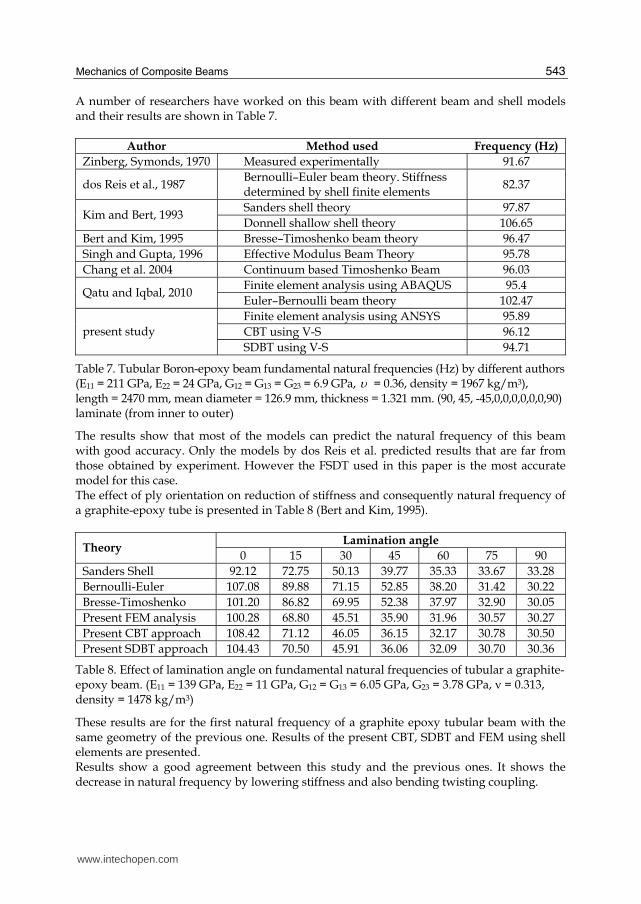
A number of researchers have worked on this beam with different beam and shell models and their results are shown in Table 7.

Author Method used Frequency (Hz)

Zinberg, Symonds, 1970 Measured experimentally 91.67

dos Reis et al., 1987 Bernoulli–Euler beam theory. Stiffness determined by shell finite elements

82.37

Sanders shell theory 97.87 Kim and Bert, 1993

Donnell shallow shell theory 106.65

Bert and Kim, 1995 Bresse–Timoshenko beam theory 96.47

Singh and Gupta, 1996 Effective Modulus Beam Theory 95.78

Chang et al. 2004 Continuum based Timoshenko Beam 96.03

Finite element analysis using ABAQUS 95.4 Qatu and Iqbal, 2010

Euler–Bernoulli beam theory 102.47

Finite element analysis using ANSYS 95.89

CBT using V-S 96.12 present study

SDBT using V-S 94.71

Table 7. Tubular Boron-epoxy beam fundamental natural frequencies (Hz) by different authors (E11 = 211 GPa, E22 = 24 GPa, G12 = G13 = G23 = 6.9 GPa, υ = 0.36, density = 1967 kg/m3), length = 2470 mm, mean diameter = 126.9 mm, thickness = 1.321 mm. (90, 45, -45,0,0,0,0,0,0,90) laminate (from inner to outer)

The results show that most of the models can predict the natural frequency of this beam with good accuracy. Only the models by dos Reis et al. predicted results that are far from those obtained by experiment. However the FSDT used in this paper is the most accurate model for this case. The effect of ply orientation on reduction of stiffness and consequently natural frequency of a graphite-epoxy tube is presented in Table 8 (Bert and Kim, 1995).

Lamination angle Theory

0 15 30 45 60 75 90

Sanders Shell 92.12 72.75 50.13 39.77 35.33 33.67 33.28

Bernoulli-Euler 107.08 89.88 71.15 52.85 38.20 31.42 30.22

Bresse-Timoshenko 101.20 86.82 69.95 52.38 37.97 32.90 30.05

Present FEM analysis 100.28 68.80 45.51 35.90 31.96 30.57 30.27

Present CBT approach 108.42 71.12 46.05 36.15 32.17 30.78 30.50

Present SDBT approach 104.43 70.50 45.91 36.06 32.09 30.70 30.36

Table 8. Effect of lamination angle on fundamental natural frequencies of tubular a graphite-epoxy beam. (E11 = 139 GPa, E22 = 11 GPa, G12 = G13 = 6.05 GPa, G23 = 3.78 GPa, ν = 0.313, density = 1478 kg/m3)

These results are for the first natural frequency of a graphite epoxy tubular beam with the same geometry of the previous one. Results of the present CBT, SDBT and FEM using shell elements are presented. Results show a good agreement between this study and the previous ones. It shows the decrease in natural frequency by lowering stiffness and also bending twisting coupling.

www.intechopen.com


544

6. Conclusion

Different approaches for static and dynamic analysis of composite beams were proposed and a modified FSDT model that accounts for various laminate couplings and shear deformation and rotary inertia was validated. The method was verified using 3D FEM model. The results showed good accuracy of the model for rectangular beams in static analysis for laminates having bending-twisting coupling and in dynamic analysis for all kinds of laminates. Also the model was verified for dynamic analysis of tubular cross section beams (or shafts) and the results were accurate compared to experimental ones and other models. This model provides an accurate approach for calculating the natural frequencies of beams and shafts with arbitrary laminate for engineers and scientists.

7. References

Qatu M. S. (2004). Vibration of Laminated Shells and Plates, Elsevier Academic Press, ISBN

978-0-08-044271-6, Netherlands.

Kaw A. K. (2005). Mechanics of Composite Materials. CRC Press, ISBN 978-084-9313-43-1,

Boca Raton, USA.

Rios, G. & Chan, W. S. (2010). A Unified Analysis of stiffened Reinforced Composite beams.

In: Proceedings of 25th ASC conference. Dayton, USA.

Vinson, J. R. & Sierakowski, R. L. (2002). The behavior of Structures Composed of

Composite Materials, Kluwer Academic Publishers, ISBN 978-140-2009-04-4,

Netherlands.

Qatu M. S. (1993). Theories and analyses of Thin and moderately Thick Laminated

Composite Curved Beams,. International Journal of Solids and Structures, Vol. 30,

No. 20, pp. 2743-2756, ISSN 0020-7683.

Timoshenko SP. (1921). On the correction for shear of the differential equation for transverse

vibrations of prismatic beams, Philos Mag, Sec 6, No. 41 pp. 744–746. ISSN: 1478-

6435

Kapania, R. K. & Raciti S. (1989). Recent Advances in Analysis of laminated beams and

plates, PART II: Vibration and Wave Propagation, AIAA Journal, Vol.27, No.7, pp.

935-946, ISSN 0001-1452.

Chidamparam, P. & Leissa A. W. (1993). Vibrations of Planar Curved Beams, Rings, and

Arches, Appl. Mech. Rev., Vol.46, No.9, pp. 467 -484, ISSN 0003-6900.

Chandrashekhara, K., Krishnamurthy, K. & Roy, S. (1990). Free vibration of composite

beams including rotary inertia and shear deformation, Composite Structures,

Vol.14, No.4, pp. 269-279, ISSN: 0263-8223.

Krishnaswamy, A., Chandrashekhara, K. & Wu, WZB. (1992). Analytical Solutions to

vibration of generally layered composite beams, Journal of Sound and Vibration,

Vol.159, No.1, pp. 85-99, ISSN: 0022-460X.

Abramovich, H. & Livshits, A. (1994). Free vibrations of non-symmetric cross ply laminated

composite beams, Journal of Sound and Vibration, Vol. 176, No. 5, pp. 597-612,

ISSN 0022-460X.

Abramovich, H., Eisenberger, M. & Shulepov, O. (1995). Vibrations of Multi-Span Non-

Symmetric Composite Beams, Composites Engineering Vol.5, No.4, pp. 397-404,

ISSN 1359-8368.

www.intechopen.com


545

Teboub, Y. & Hajela, P. (1995). Free vibration of generally layered composite beams using

symbolic computation, Composite Structures, Vol.33, No.3, pp. 123-134, ISSN: 0263-

8223.

Banerjee, J. R. Williams F. W. (1995). Free Vibration of Composite Beams—an Exact Method

Using Symbolic Computation, AIAA Journal of Aircraft, Vol. 32, No.3, pp. 636-642,

ISSN 0021-8669.

Banerjee, J. R. (2001). Explicit analytical expressions for frequency equation and mode

shapes of composite beams, International Journal of Solids and Structures, Vol.38,

No.14, pp. 2415-2426, ISSN 0020-7683.

Li, J., Shen, R., Hua, H. & Jin, J. (2004). Bending–torsional coupled dynamic response of

axially loaded composite Timosenko thin-walled beam with closed cross-section,

Composite Structures, Vol.64, No.1, pp. 23–35, ISSN 0263-8223.

Eisenberger, M., Abramovich, H. & Shulepov, O. (1995). Dynamic stiffness analysis of

laminated beams using a first order shear deformation theory. Composite

Structures, Vol.31, No.4, pp. 265-271, ISSN 0263-8223.

Khdeir, A. A. & Reddy, J. N. (1997). Free And Forced Vibration Of Cross-Ply Laminated

Composite Shallow Arches. Intl J Solids Structures, Vol.34, No.10, pp. 1217-1234,

ISSN 0020-7683.

Kant, T., Marur, S. R. & Rao, G. S. (1998). Analytical solution to the dynamic analysis of

laminated beams using higher order refined theory. Composite Structures, Vol.40,

No.1, pp. 1-9, ISSN 0263-8223.

Matsunaga, H. (2001). Vibration and Buckling of Multilayered Composite Beams According

to Higher Order Deformation Theories, Journal of Sound and vibration, Vol.246,

No.1, pp. 47-62, ISSN 0022-460X.

Subramanian, P. (2006). Dynamic analysis of laminated composite beams using higher order

theories and finite elements, Composite Structures, Vol.73, No.3, pp. 342-353, ISSN

0263-8223.

Kapuria, S., Dumir, P.C. & Jain, N. K. (2004). Assessment of zigzag theory for static loading,

buckling, free and forced response of composite and sandwich beams. Composite

Structures, Vol.64, No.3-4, pp. 317–27, ISSN 0263-8223.

Zhen, W. & Wanji, C. (2008). An assessment of several displacement based theories for the

vibration and stability analysis of laminated composite and sandwich beams,

Composite Structures, Vol.84, No.4, pp. 337-349, ISSN 0263-8223.

Zinberg, H. & Symonds, M.F. (1970). The development of an advanced composite tail rotor

driveshaft. In: Proceedings of 26th annual forum of the American Helicopter

Society, Washington, USA.

dos Reis, H. L. M., Goldman, R. B. & Verstrate, P. H. (1987). Thin-walled laminated

composite cylindrical tubes. Part III––critical speed analysis, Journal of Composite

Technology and Research, Vol.9, No.2, pp. 58–62, ISSN 0884-6804.

Kim, C. D. Bert, C. W. (1993). Critical speed analysis of laminated composite hollow drive

shafts. Composite Engineering, Vol.3, No.7-8, pp. 633–43, ISSN: 1359-8368.

Bert, C. W. & Kim, C. (1995) Whirling of composite-material driveshafts including bending–

twisting coupling and transverse shear deformation, Journal of Vibration and

Acoustics, Vol.117, No.1, pp. 17–21, ISSN 1048-9002.

www.intechopen.com


546

Singh, S. P. & Gupta, K. (1996). Composite shaft rotordynamic analysis using a layerwise theory, Journal of Sound and Vibration, Vol. 191, No. 5, pp. 739–56, ISSN 0022-460X.

Chang, M-Y., Chen, JK. & Chang, C-Y. (2004). A simple spinning laminated composite shaft model, International Journal of Solids and Structures, Vol.41, No.3-4, pp. 637–62, ISSN 0020-7683.

Qatu, M. S. & Iqbal, J. (2010). Transverse vibration of a two-segment cross-ply composite shafts with a lumped mass, Composite Structures, Vol.92, No.5, pp. 1126-1131, ISSN 0263-8223.

www.intechopen.com

Advances in Composite Materials - Analysis of Natural and Man-Made MaterialsEdited by Dr. Pavla Tesinova

ISBN 978-953-307-449-8Hard cover, 572 pagesPublisher InTechPublished online 09, September, 2011Published in print edition September, 2011

InTech EuropeUniversity Campus STeP Ri Slavka Krautzeka 83/A 51000 Rijeka, Croatia Phone: +385 (51) 770 447 Fax: +385 (51) 686 166www.intechopen.com

InTech ChinaUnit 405, Office Block, Hotel Equatorial Shanghai No.65, Yan An Road (West), Shanghai, 200040, China

Phone: +86-21-62489820 Fax: +86-21-62489821

Composites are made up of constituent materials with high engineering potential. This potential is wide as wideis the variation of materials and structure constructions when new updates are invented every day.Technological advances in composite field are included in the equipment surrounding us daily; our lives arebecoming safer, hand in hand with economical and ecological advantages. This book collects original studiesconcerning composite materials, their properties and testing from various points of view. Chapters are dividedinto groups according to their main aim. Material properties are described in innovative way either for standardcomponents as glass, epoxy, carbon, etc. or biomaterials and natural sources materials as ramie, bone, wood,etc. Manufacturing processes are represented by moulding methods; lamination process includes monitoringduring process. Innovative testing procedures are described in electrochemistry, pulse velocity, fracturetoughness in macro-micro mechanical behaviour and more.

How to referenceIn order to correctly reference this scholarly work, feel free to copy and paste the following:

Mehdi Hajianmaleki and Mohammad S. Qatu (2011). Mechanics of Composite Beams, Advances in CompositeMaterials - Analysis of Natural and Man-Made Materials, Dr. Pavla Tesinova (Ed.), ISBN: 978-953-307-449-8,InTech, Available from: http://www.intechopen.com/books/advances-in-composite-materials-analysis-of-natural-and-man-made-materials/mechanics-of-composite-beams

© 2011 The Author(s). Licensee IntechOpen. This chapter is distributedunder the terms of the Creative Commons Attribution-NonCommercial-ShareAlike-3.0 License, which permits use, distribution and reproduction fornon-commercial purposes, provided the original is properly cited andderivative works building on this content are distributed under the samelicense.

https://creativecommons.org/licenses/by-nc-sa/3.0/