
McGraw-Hill/Irwin
©2008 The McGraw-Hill Companies, All Rights Reserved
Aggregate Demand
Chapter 9
2
Chapter 9 – Aggregate Demand
1. Consumption.
2. The Consumption Function.
3. Investment.
4. Government & Net Export Spending.
5. Macro Failure.
6. Anticipating AD Shifts.

5
Some Quick
Review:

6
Macro Equilibrium
AS and AD combine to determine macro equilibrium.
Equilibrium is established where AS and AD intersect.
e
PR
ICE
LE
VE
L
REAL OUTPUT (quantity per year)QE
PE
Aggregatedemand
Aggregatesupply
E
7
The Desired Adjustment
Any particular macro equilibrium point may be undesirable.
All economists agree that short-run unemployment is possible.
Will the economy self-adjust ?
If not, government might have to step in to increase AD to reach full employment.
8
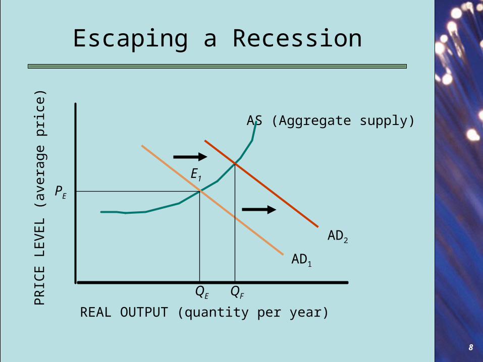
Escaping a Recession
AS (Aggregate supply)
AD1
E1
REAL OUTPUT (quantity per year)
PRIC
E LE
VEL
(ave
rage
pric
e)
AD2
QFQE
PE

9
…New Stuff…

10
1. Consumption
11
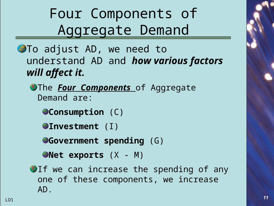
Four Components of Aggregate Demand
To adjust AD, we need to understand AD and how various factors will affect it.
The Four Components of Aggregate Demand are:
Consumption (C)
Investment (I)
Government spending (G)
Net exports (X - M)
If we can increase the spending of any one of these components, we increase AD.
LO1

12
Building an AD Curve
13
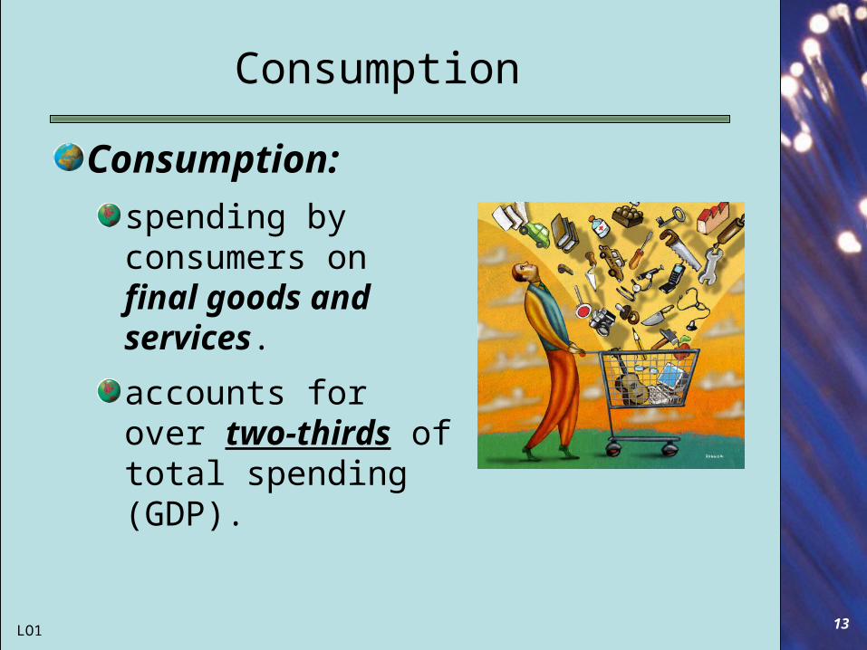
Consumption
Consumption:
spending by consumers on final goods and services.
accounts for over two-thirds of total spending (GDP).
LO1
14
Income and Consumption
Consumers tend to spend most of their disposable incomes.
(Disposable income:
- the after-tax income of consumers:
- personal income less personal taxes.)
LO1
15
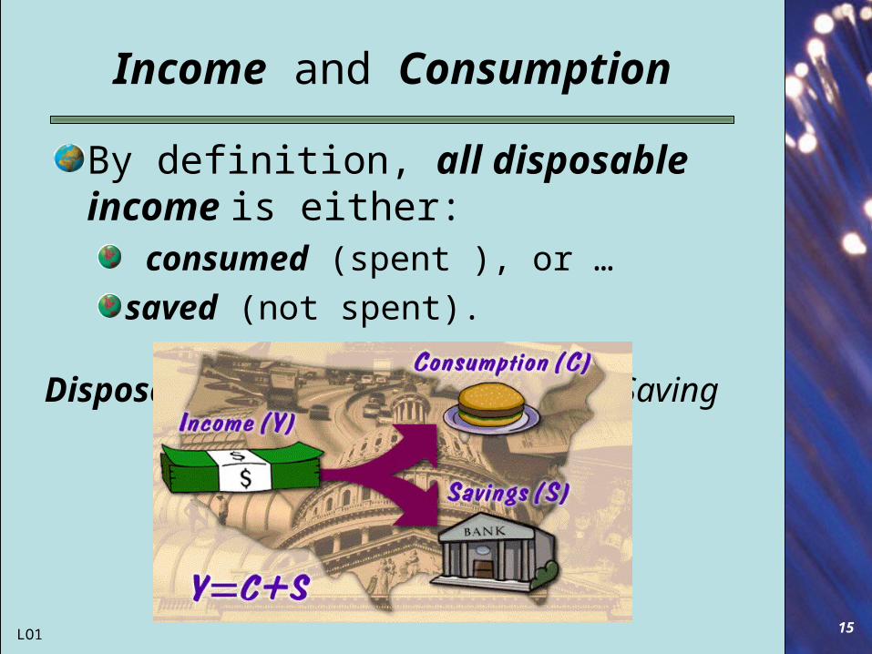
Income and Consumption
By definition, all disposable income is either:
consumed (spent ), or …
saved (not spent).
Disposable income = Consumption + Saving
LO1
YD = C + S

16
U.S. Consumption and Income
DISPOSABLE INCOME (billions of dollars per year)
$1000 2000 3000 4000
Actual consumer spending
6000
5000
4000
3000
2000
1000
0 5000 6000 7000
45°
$7000
19801982
19841986
19881990
19921994
19961998
1999
2000
CONS
UMPT
ION
(billi
ons
of d
olla
rs p
er y
ear)
C = YD
LO1

17
Income, Consumption, & AD
If we can model consumer spending…
…then we can predict consumer spending…
… and more effectively manipulate the AD curve.

18
Keynes described the consumption-income relationship in two ways:
1. AVERAGE propensity to consume:
- “APC"
2. MARGINAL propensity to consume:
- “MPC"
Income, Consumption, & AD
LO1
19
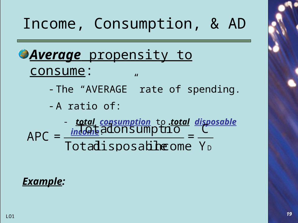
Income, Consumption, & AD
Average propensity to consume:- The “AVERAGE” rate of spending.
- A ratio of:
- total consumption to total disposable income:
LO1
Example:

20
Average Propensity to Save
Average Propensity to Save:
LO1
Example:
21
APC v. APS
So…
Since YD = C + S…
- or -
Example:
22
Marginal Propensity to Consume
2. Marginal propensity to consume:
- The ratio of:
- changes in consumption to changes in disposable income.
- The fraction of each additional (marginal) dollar of disposable income spent on consumption.
LO1

23
Marginal Propensity to Consume
Marginal Propensity to Consume:
MPC =Change in Consumption
Change in Disposable Income=
C
YD
LO1
8.10
8
200-210
192-200=
Y
C=MPC
D
Example:
24
Marginal Propensity to Save
Marginal propensity to save:the fraction of each additional (marginal) dollar of disposable income not spent on consumption.
LO1
Example:
25
MPC vs. MPS
YD = C + S
So…
Example:
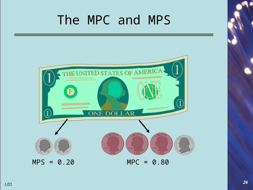
26
The MPC and MPS
MPS = 0.20 MPC = 0.80
LO1

27
ReviewIf the MPC is .90 and the APC is .95:
1. What is the APS?
2. What is the MPS?
3. What is the level of spending if disposable income (Yd) is $600?
4. How much would be saved from an additional $100 of disposable income.
5. What are the four components of AD?
.05
.1
$570
$10
C, I, G, (X-M)
28
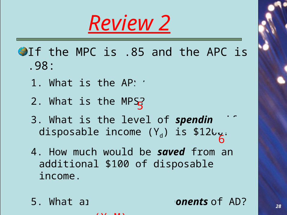
Review 2If the MPC is .85 and the APC is .98:
1. What is the APS?
2. What is the MPS?
3. What is the level of spending if disposable income (Yd) is $1200?
4. How much would be saved from an additional $100 of disposable income.
5. What are the four components of AD?
.02
.15
$1176
$15
C, I, G, (X-M)
29
2. The Consumption Function
30
The Consumption Function
The consumption function:
a mathematical relationship that helps predict consumer behavior.
Based in part on the concept of marginal propensity to consume.
LO1

31
The Consumption Function
Keynes distinguished two kinds of consumer spending.
Autonomous:
Spending not influenced by current income,
Income-dependent:
Spending that is determined by current income.
LO1

32
The Consumption Function
These two determinants of consumption are summarized in an equation called the consumption function.
Income -
dependent consumption
Autonomous consumption
Total consumption
LO1
(***Informal, “theoretical” equation: not the mathematical equation!)

33
Autonomous Consumption
Autonomous consumption:-consumption that occurs independent of income level.
Autonomous determinants of consumption include:
Expectations.
Wealth.
Credit.
(Taxes) ?!?
LO1
34
Expectations
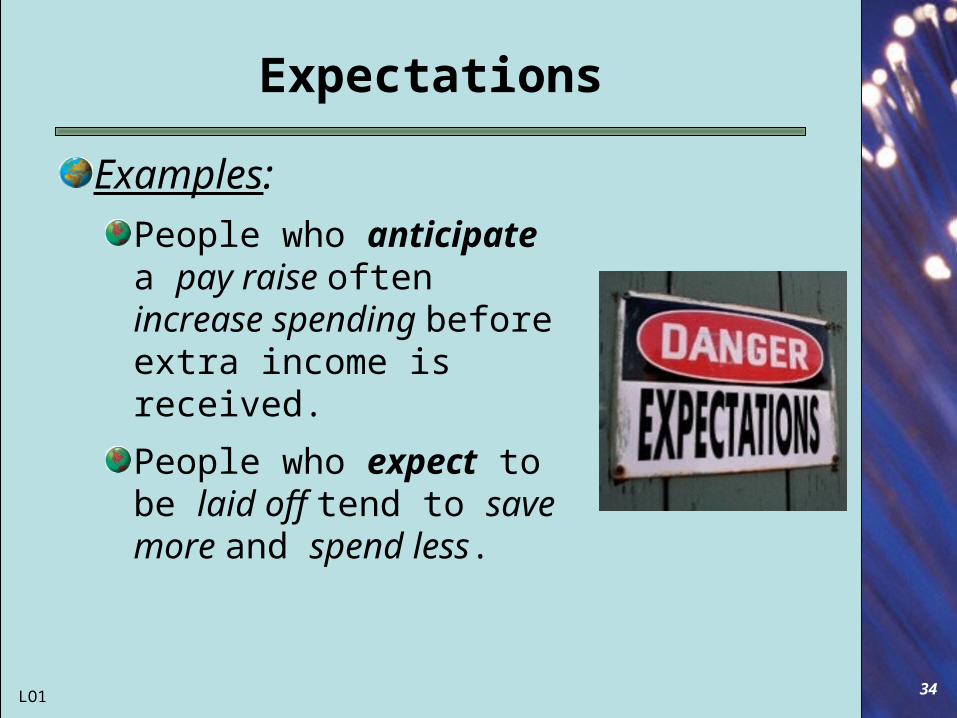
Examples:
People who anticipate a pay raise often increase spending before extra income is received.
People who expect to be laid off tend to save more and spend less.
LO1

35
Wealth
An individual’s wealth affects his willingness and ability to consume.
The wealth effect:a change in consumer spending…
…caused by…
a change in the value of owned assets.
LO1
36
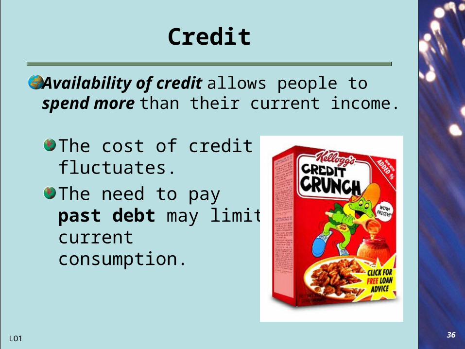
Credit
The cost of credit fluctuates.
The need to pay past debt may limit current consumption.
Availability of credit allows people to spend more than their current income.
LO1

38
Income-Dependent Consumption
Income-dependent consumption:This is delineated by one’s marginal propensity to consume (MPC):
MPC x Disposable Income

39
The Consumption Function
The consumption function:
The mathematical relationship indicating the (desired) rate of consumer spending at various income levels.
It combines autonomous and income-dependent consumption into one formula.
It provides a precise basis for predicting how changes in income (YD) affect consumer spending (C) …
…and therefore, AD!LO1

43
The Consumption Function
C = a + bYD
where: C = current consumption a = autonomous consumption b = marginal propensity to consumeYD = disposable income
LO1
Income -dependent
consumption
Autonomous consumption
Total consumption

44
The Consumption Function

46
Consumer Behavior
Even with an income level of zero:
there will be some consumption (autonomous).
Consumption will rise with income based on the MPC.
Slope = MPC.
LO1

47
Consumer Behavior
Dissaving:
current consumption exceeds current income
a negative saving flow.
LO1

48
Justin’s Consumption Function
LO1
49
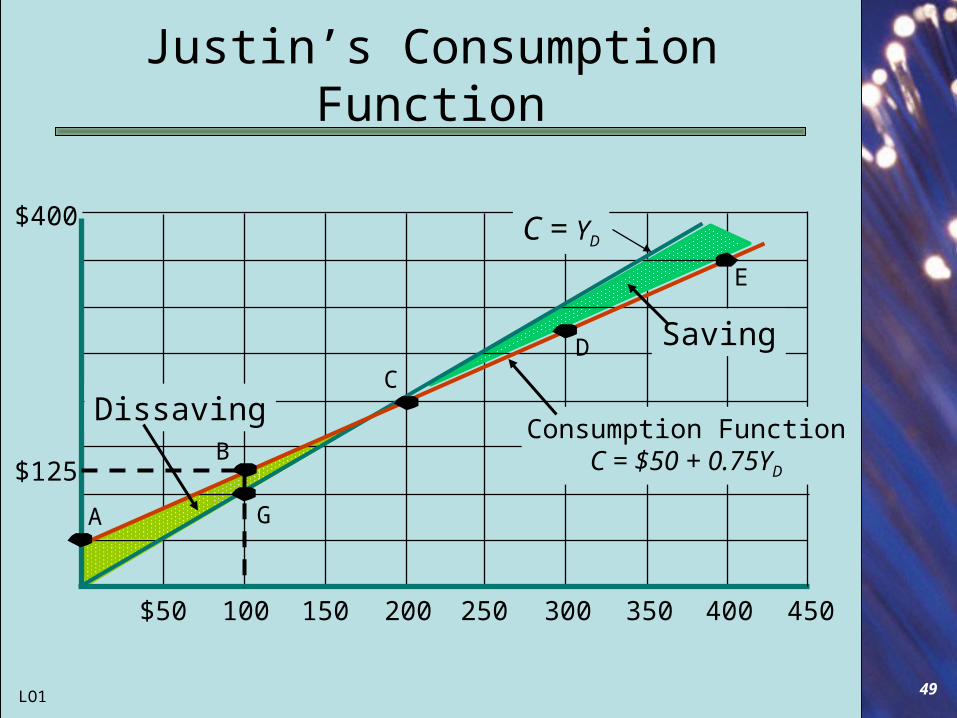
Justin’s Consumption Function
$400
$50 100 150 200 250 300 350 400 450
C = YD
Saving
DissavingConsumption Function
C = $50 + 0.75YD$125
A
CD
E
B
G
LO1
51
Application
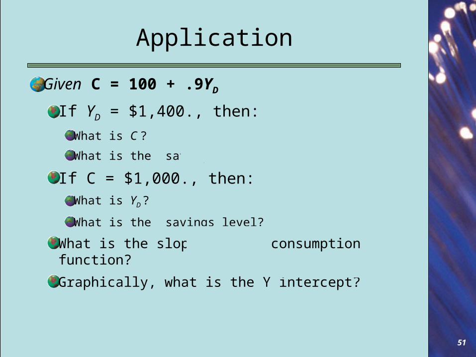
Given C = 100 + .9YD
If YD = $1,400., then:
What is C ?
What is the savings level?
If C = $1,000., then:What is YD ?
What is the savings level?
What is the slope of this consumption function?
Graphically, what is the Y intercept?
$1,360
$40
$1,000
$0.00

52
Application
2. Suppose the MPC in an economy is 0.7. The APC is initially 0.8 and disposable income is $10 billion. If disposable income increases to $14 billion, what is the new level of consumption?
A). $10.8 billion. C). $8 billion.
B). $11.2 billion. D). $12.8 billion.

53
Shifts of the Consumption Function
Changing the a or b values in the consumption function (C = a + bYD) will shift the function to a new position.
A change in the a variable will cause a parallel shift of the function.
Caused by changes in expectations, wealth, or credit.
LO1
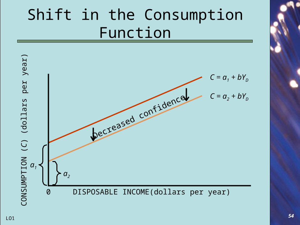
54
Shift in the Consumption Function
a1
C = a1 + bYD
C = a2 + bYD
a2CONS
UMPT
ION
(C) (
dolla
rs p
er y
ear)
DISPOSABLE INCOME(dollars per year)0
Decreased confidence
LO1

55
Shifts of Aggregate Demand
Shifts in the consumption function:
are reflected in shifts of AD:
Consumption function ↑ = AD to the right:
Consumption function ↓ = AD to the left:
LO2

57
AD Effects of Consumption Shifts
Y0
f2
f1
Q2 Q1
P1
C1
AD1
Shift = f1 – f2
Expenditure
Income
C2
Price Level
Real Output
AD2
LO2
***The AD curve will shift if:
- autonomous consumption changes, or…
- consumer incomes change.

61
Shifts and Cycles
AD shifts may originate from consumer behavior.
AD shifts = macro instability.
LO2

63
3. Investment

64
Investment
Investment:expenditures on (production of) new plant, equipment, and structures (capital), …
in a given time period, …
plus changes in business inventories.
LO1

65
Determinants of Investment
The following factors determine the amount of investment that occurs in an economy:
Interest rates.
Expectations.
Technology and innovation.
LO1
66
Interest Rates
Businesses typically borrow money to invest in new plants or equipment.
The higher the interest rate, the costlier it is to invest and the lower the investment spending.
LO1

67
Investment Demand
11
Inte
rest
Rat
e (p
erce
nt p
er y
ear)
Planned Investment Spending (billions of dollars per year)
100 200 300 400 500
10
9
8
7
6
54
3
2
1
0
11
B
A
LO1

68
Expectations
Expectations: play a critical role in investment decisions.
are determined by business confidence in future sales.
Confidence ↑ = AD shift to the right.
LO1

69
Investment Demand
11
Inte
rest
Rat
e (p
erce
nt p
er y
ear)
Planned Investment Spending (billions of dollars per year)
100 200 300 400 500
10
9
8
7
6
54
3
2
1
0
C
I2
I3
11
Better expectations
B
A
Initial expectations
Worse expectations
LO1

70
Technology and Innovation
New technology changes the demand for investment goods:
Technological advances and corresponding cost reductions stimulate new investment spending.
LO1

71
Investment Demand
11
Inte
rest
Rat
e (p
erce
nt p
er y
ear)
Planned Investment Spending (billions of dollars per year)
100 200 300 400 500
10
9
8
7
6
54
3
2
1
0
I2
11
Investment demand givenavailability of new technology
B
A
Initial Investment Demand
LO1

72
AD Shifts
So….The AD curve shifts:
to the left when investment spending declines.
to the right when investment spending increases.
LO2

73
AD Effects of Consumption Shifts
Q2 Q1
AD1
Price Level
Real Output
AD2
LO2
The AD curve shifts:
to the left when investment spending declines.
to the right when investment spending increases.
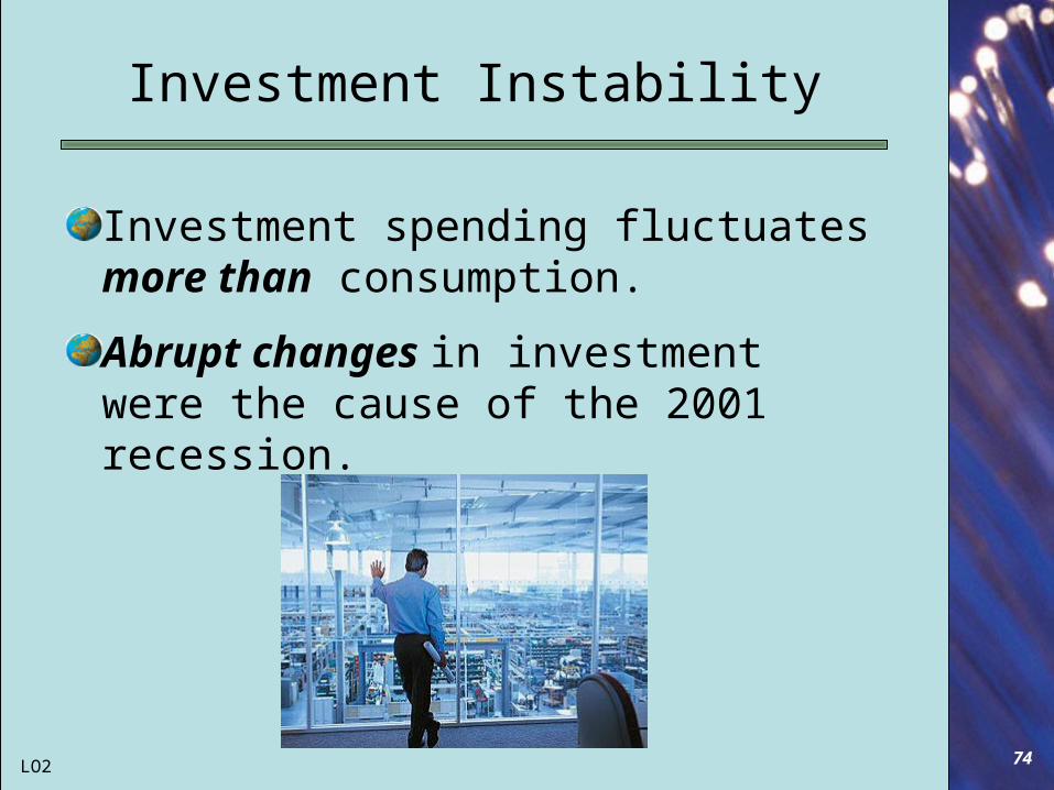
74
Investment Instability
Investment spending fluctuates more than consumption.
Abrupt changes in investment were the cause of the 2001 recession.
LO2

75
Volatile Investment Spending
LO2

76
4. Government Spending and Net Export Spending
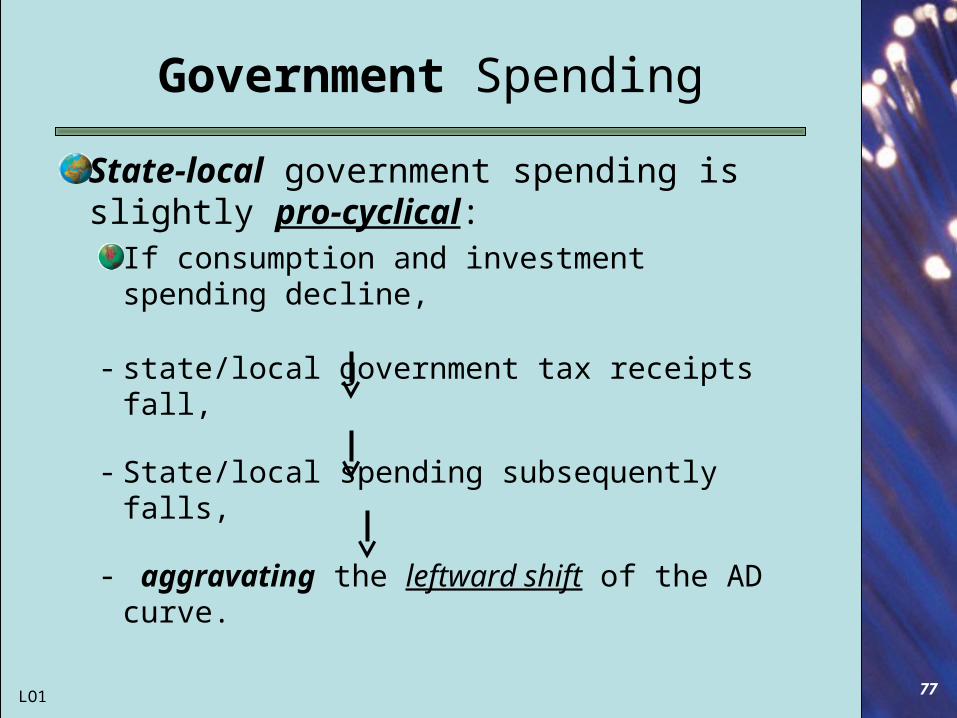
77
Government Spending
State-local government spending is slightly pro-cyclical:
If consumption and investment spending decline,
- state/local government tax receipts fall,
- State/local spending subsequently falls,
- aggravating the leftward shift of the AD curve.
LO1

78
Government Spending
The federal government can “deficit spend:
it has counter-cyclical power.
can increase spending to counteract declines in consumption and investment spending.
LO1

79
Net Exports
Net exports can be both uncertain and unstable, creating further shifts of aggregate demand.
LO1

80
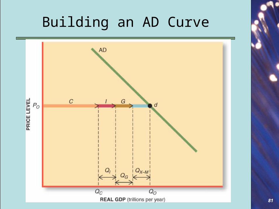
So…The four components of spending (C+I+G+(X-M)) come together to determine aggregate demand.
By adding up the intended spending of these market participants we can see how much output will be demanded at the current price level.
LO1
81
Building an AD Curve

82
Review
1. Suppose a consumption function is given as C = $175 + 0.85YD. The marginal propensity to save is:
2. If an increase in disposable income causes consumption to increase from $4,000 to $10,000 and causes saving to increase from $2,000 to $4,000 it can be inferred that the MPC equals:
3. Suppose the consumption function is C = $300 + 0.9YD. If disposable income is $400, consumption is:
What is the level of savings?
83
ReviewWhat are the 3 determinants of investment spending?
What is the major difference between Federal v. state/local spending (demand) during a recession?

84
Application
2. Suppose the MPC in an economy is 0.7. The APC is initially 0.8 and disposable income is $10 billion. If disposable income increases to $14 billion, what is the new level of consumption?
A). $10.8 billion. C). $8 billion.
B). $11.2 billion. D). $12.8 billion.

85
5. Macro Failure
86
Macro Failure - REVIEW
There are two chief concerns about macro equilibrium:
Undesirability:The market’s macro-equilibrium might not give us full employment or price stability.
Instability:Even if the market’s macro-equilibrium were at full employment and price stability, it might not last.
LO3

88
Recessionary GDP Gap
(REVIEW): Keynes worried that equilibrium GDP may not occur at full-employment GDP.
Equilibrium GDP: is the value of total output (real GDP) produced at macro equilibrium (AS=AD).
Full-employment GDP: is the value of total output (real GDP) produced at full employment.
LO3

89
Macro Failures
PRICE LEVEL
REAL GDP
Macro Success: (perfect AD)
AD1
AS
P*E1
QF
LO3
90
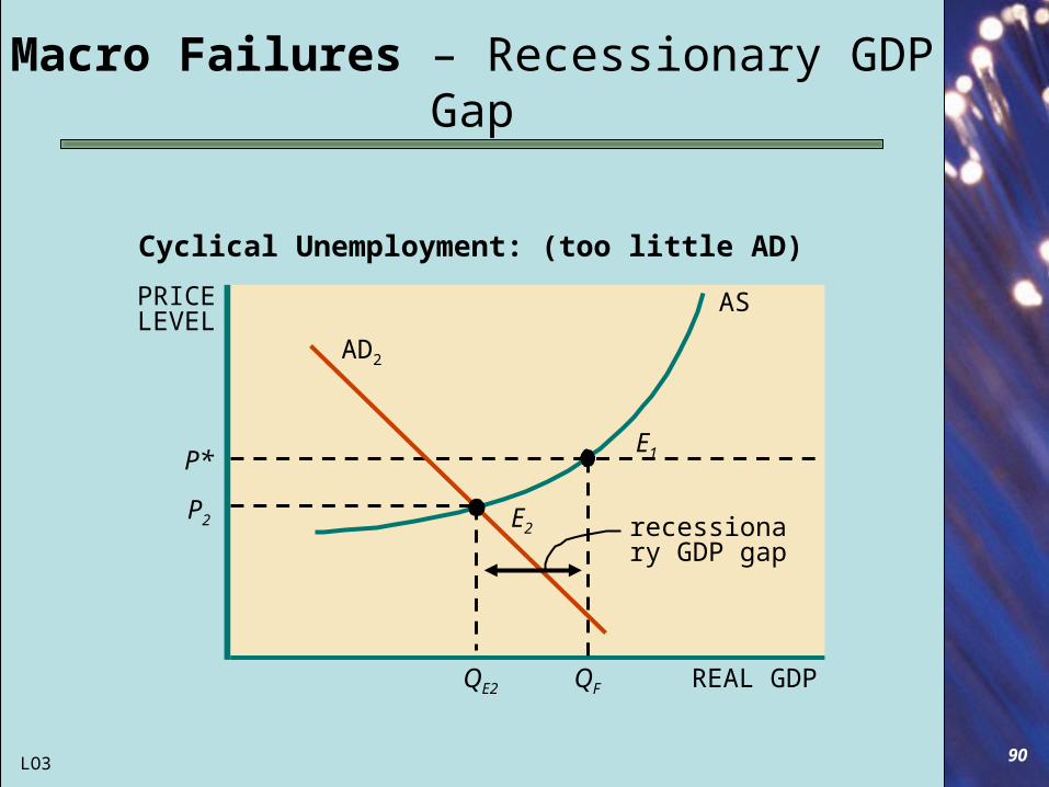
Macro Failures – Recessionary GDP Gap
PRICE LEVEL
REAL GDP
Cyclical Unemployment: (too little AD)
AS
P*E1
QF
AD2
E2P2
QE2
recessionary GDP gap
LO3
91
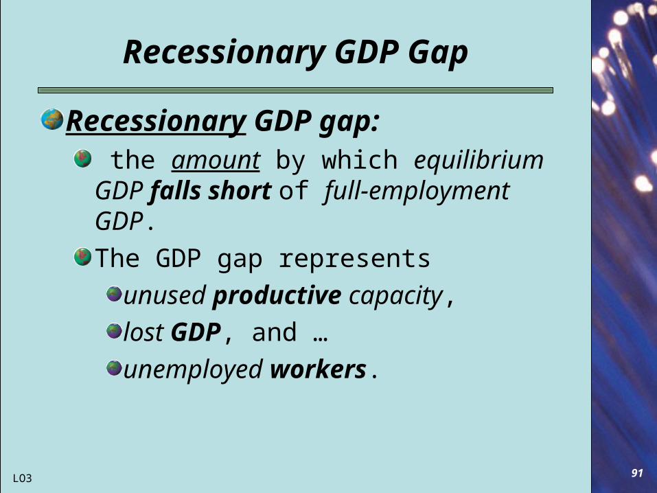
Recessionary GDP Gap
Recessionary GDP gap: the amount by which equilibrium GDP falls short of full-employment GDP.
The GDP gap represents
unused productive capacity,
lost GDP, and …
unemployed workers.
LO3

94
A Recessionary GDP Gap
LO3

95
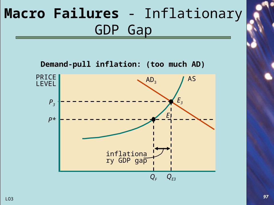
Inflationary GDP Gap
Inflationary GDP gap:
the amount by which equilibrium GDP exceeds full-employment GDP.
leads to demand-pull inflation:
an increase in the price level initiated by excessive aggregate demand.
LO3
97
Macro Failures - Inflationary GDP Gap
PRICE LEVEL
Demand-pull inflation: (too much AD)
AS
P*E1
QF
AD3
E3P3
QE3
inflationary GDP gap
LO3
99
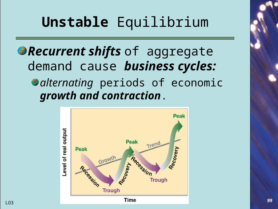
Unstable Equilibrium
Recurrent shifts of aggregate demand cause business cycles:
alternating periods of economic growth and contraction.
LO3
101
Self-Adjustment?
The critical question is whether undesirable outcomes will persist.
Classical economists asserted that markets self-adjust so that macro failures would be temporary.
Keynes didn’t think that was likely to happen.

102
6. Anticipating AD Shifts

103
Looking for AD Shifts
Average workweek.Unemployment claims.Delivery times.Credit.Materials prices.Equipment orders.
Stock prices.
Money supply.
New orders.
Building permits.
Inventories.
Policymakers use the Index of Leading Indicators to forecast changes in GDP:

104
Looking for AD Shifts

McGraw-Hill/Irwin
©2008 The McGraw-Hill Companies, All Rights Reserved
Aggregate Demand
End of Chapter 9
Recommended