MATHEMATICS
BOOK FOR MSQE
Further Reading Lists for MSQE & Other Entrances:
1. Mathematics for Economic Analysis by Sydsaeter Hammond 2. Mathematical Statistics by Gupta Kapoor 3. Basic Econometrics by Gujarati 4. Microeconomics by Satya Ranjan Chakraborty 5. Microeconomics by Hal Varian/Nicholson & Synder 6. Macroeconomics by H.L. Ahuja 7. Macroeconomics by Dornbusch & Fischer/Branson 8. Development Economics by Debraj Ray 9. Indian Economy by Sundaram &Dutt 10. An Introduction to Game Theory by Osborne
AL
GE
BR
A
2
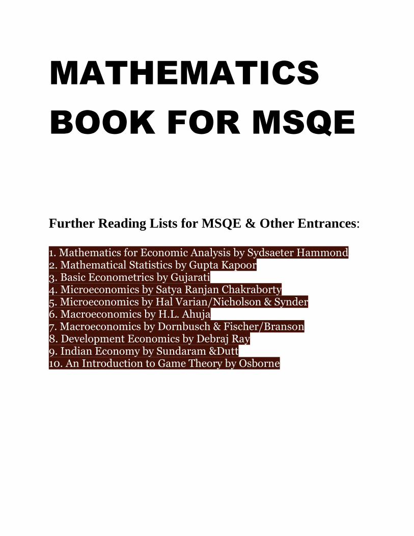
Arithmetic series
General (kth) term, uk
= a + (k – 1)d
last (nth) term, l = un
= a + (n – l)d
Sum to n terms, Sn
= n(a + l) = n[2a + (n – 1)d]
Geometric series
General (kth) term, uk
= a rk–1
Sum to n terms, Sn
= =
Sum to infinity S∞ = , – 1 < r < 1
Binomial expansions
When n is a positive integer
(a + b)n = an + ( ) an –1 b + ( ) an–2 b2 + ... + ( ) an–r br + ... bn , n ∈ N
where
( ) =nC
r= ( ) + ( ) = ( )
General case
(1 + x)n = 1 + nx + x2 + ... + xr + ... , |x| < 1,
n ∈ R
Logarithms and exponentials
exln a = ax loga
x =
Numerical solution of equations
Newton-Raphson iterative formula for solving f(x) = 0, xn+1
= xn
–
Complex Numbers
{r(cos θ + j sin θ)}n = rn(cos nθ + j sin nθ)
ejθ = cos θ + j sin θThe roots of zn = 1 are given by z = exp( j) for k = 0, 1, 2, ..., n–1
Finite series
∑n
r=1
r2 = n(n + 1)(2n + 1) ∑n
r=1
r3 = n2(n + 1)21–4
1–6
2πk–––– n
f(xn)
––––f '(x
n)
logbx
–––––log
ba
n(n – 1) ... (n – r + 1)–––––––––––––––––
1.2 ... r
n(n – 1)–––––––
2!
n + 1r + 1
nr + 1
nr
n!––––––––r!(n – r)!
nr
nr
n2
n1
a–––––1 – r
a(rn – 1)––––––––
r – 1
a(1 – rn)––––––––
1 – r
1–2
1–2
Infinite series
f(x) = f(0) + xf '(0) + f"(0) + ... + f (r )(0) + ...
f(x) = f(a) + (x – a)f '(a) + f"(a) + ... + + ...
f(a + x) = f(a) + xf '(a) + f"(a) + ... + f(r)(a) + ...
ex = exp(x) = 1 + x + + ... + + ... , all x
ln(1 + x) = x – + – ... + (–1)r+1 + ... , – 1 < x < 1
sin x = x – + – ... + (–1)r + ... , all x
cos x = 1 – + – ... + (–1)r + ... , all x
arctan x = x – + – ... + (–1)r + ... , – 1 < x < 1
sinh x = x + + + ... + + ... , all x
cosh x = 1 + + + ... + + ... , all x
artanh x = x + + + ... + + ... , – 1 < x < 1
Hyperbolic functions
cosh2x – sinh2x = 1, sinh2x = 2sinhx coshx, cosh2x = cosh2x + sinh2x
arsinh x = ln(x + ), arcosh x = ln(x + ), x > 1
artanh x = ln ( ), |x| < 1
Matrices
Anticlockwise rotation through angle θ, centre O: ( )Reflection in the line y = x tan θ : ( )cos 2θ sin 2θ
sin 2θ –cos 2θ
cos θ –sin θsin θ cos θ
1 + x–––––1 – x
1–2
x2 1–x2 1+
x2r+1––––––––(2r + 1)
x5––5
x3––3
x2r––––(2r)!
x4––4!
x2––2!
x2r+1––––––––(2r + 1)!
x5––5!
x3––3!
x2r+1––––––2r + 1
x5––5
x3––3
x2r––––(2r)!
x4––4!
x2––2!
x2r+1––––––––(2r + 1)!
x5––5!
x3––3!
xr––r
x3––3
x2––2
xr––r!
x2––2!
xr––r!
x2––2!
(x – a)rf(r)(a)––––––––––r!
(x – a)2––––––
2!
xr––r!
x2––2!
3
TR
IGO
NO
ME
TR
Y, V
EC
TO
RS
AN
D G
EO
ME
TR
Y
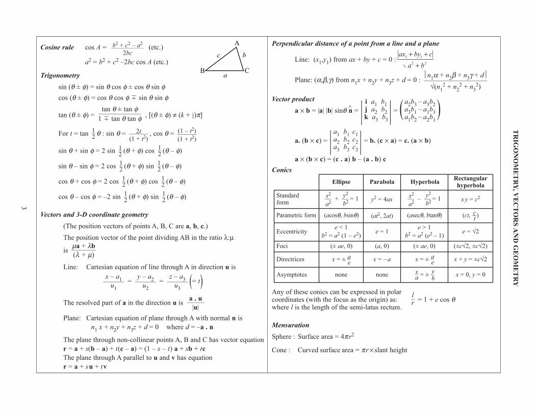
Cosine rule cos A = (etc.)
a2 = b2 + c2 –2bc cos A (etc.)
Trigonometry
sin (θ ± φ) = sin θ cos φ ± cos θ sin φcos (θ ± φ) = cos θ cos φ 7 sin θ sin φ
tan (θ ± φ) = , [(θ ± φ) ≠ (k + W)π]
For t = tan θ : sin θ = , cos θ =
sin θ + sin φ = 2 sin (θ + φ) cos (θ – φ)
sin θ – sin φ = 2 cos (θ + φ) sin (θ – φ)
cos θ + cos φ = 2 cos (θ + φ) cos (θ – φ)
cos θ – cos φ = –2 sin (θ + φ) sin (θ – φ)
Vectors and 3-D coordinate geometry
(The position vectors of points A, B, C are a, b, c.)
The position vector of the point dividing AB in the ratio λ:µ
is
Line: Cartesian equation of line through A in direction u is
= = (= t)
The resolved part of a in the direction u is
Plane: Cartesian equation of plane through A with normal n is
n1
x + n2y + n
3z + d = 0 where d = –a . n
The plane through non-collinear points A, B and C has vector equation
r = a + s(b – a) + t(c – a) = (1 – s – t) a + sb + tc
The plane through A parallel to u and v has equation
r = a + su + tv
a . u–––––
|u|
z – a3––––––
u3
y – a2––––––
u2
x – a1––––––
u1
µa + λb–––––––(λ + µ)
1–2
1–2
1–2
1–2
1–2
1–2
1–2
1–2
(1 – t2)––––––(1 + t2)
2t––––––(1 + t2)
1–2
tan θ ± tan φ––––––––––––1 7 tan θ tan φ
b2 + c2 – a2––––––––––
2bc
Perpendicular distance of a point from a line and a plane
Line: (x1,y
1) from ax + by + c = 0 :
Plane: (α,β,γ) from n1x + n
2y + n
3z + d = 0 :
Vector product
a × b = |a| |b| sinθ n = | | = ( )
a. (b × c) = | | = b. (c × a) = c. (a × b)
a × (b × c) = (c . a) b – (a . b) c
Conics
Any of these conics can be expressed in polarcoordinates (with the focus as the origin) as: = 1 + e cos θwhere l is the length of the semi-latus rectum.
Mensuration
Sphere : Surface area = 4πr2
Cone : Curved surface area = πr × slant height
l–r
a1
b1
c1
a2
b2
c2
a3
b3
c3
a2b
3– a
3b
2a
3b
1– a
1b
3a
1b
2– a
2b
1
i a1
b1
j a2
b2
k a3
b3
n1α + n
2β + n
3γ + d
––––––––––––––––––√(n
12 + n
22 + n
32)
Rectangularhyperbola
HyperbolaParabolaEllipse
Standardform
–– + –– = 1 –– – –– = 1 x y = c2y2 = 4ax
Parametric form (acosθ, bsinθ) (at2, 2at) (asecθ, btanθ) (ct, ––)
Eccentricitye < 1
b2 = a2 (1 – e2)
e > 1
b2 = a2 (e2 – 1)e = 1 e = √2
Foci (± ae, 0) (a, 0) (±c√2, ±c√2)(± ae, 0)
Directrices x = ± – x = ± – x + y = ±c√2x = – a
Asymptotes none none – = ± – x = 0, y = 0
x2
a2
x2
a2
y2
b2
y2
b2
ct
ae
ae
xa
yb
ax by c
a b
1 1
2 2
+ ++
A
a
bc
CB
CA
LC
UL
US
4
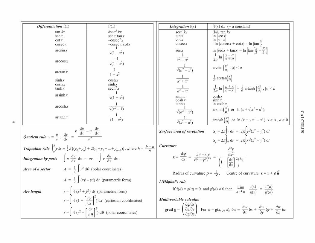
Surface area of revolution Sx
= 2π∫y ds = 2π∫y√(x2 + y2) dt
Sy
= 2π∫x ds = 2π∫x√(x2 + y2) dt
Curvature
κ = = =
Radius of curvature ρ = , Centre of curvature c = r + ρ n
L'Hôpital’s rule
If f(a) = g(a) = 0 and g'(a) ≠ 0 then =
Multi-variable calculus
grad g = ( ) For w = g(x, y, z), δw = δx + δy + δz∂w–––∂z
∂w–––∂y
∂w–––∂x
∂g/∂x
∂g/∂y
∂g/∂z
f '(a)––––g'(a)
f(x)––––g(x)
Limx➝a
1––κ
d2y–––dx2
–––––––––––––dy(1 + [––]
2
)3/2
dx
x ÿ – x y––––––––(x2 + y2)
3/2
dψ–––ds
Differentiation f(x) f '(x)
tan kx ksec2 kxsec x sec x tan xcot x –cosec2 xcosec x –cosec x cot x
arcsin x
arccos x
arctan x
sinh x cosh xcosh x sinh xtanh x sech2 x
arsinh x
arcosh x
artanh x
Quotient rule y = , =
v – u
Trapezium rule ∫b
aydx ≈ h{(y
0+ y
n) + 2(y
1+ y
2+ ... + y
n–1)}, where h =
Integration by parts ∫ u dx = uv – ∫ v dx
Area of a sector A = ∫ r2 dθ (polar coordinates)
A = ∫ (xy – yx) dt (parametric form)
Arc length s = ∫ √ (x2 + y2) dt (parametric form)
s = ∫ √ (1 + [ ]2
) dx (cartesian coordinates)
s = ∫ √ (r2 + [ ]2
) dθ (polar coordinates)dr
–––dθ
dy–––dx
1–2
1–2
du–––dx
dv–––dx
b – a–––––n1–2
dv–––dx
du–––dxdy
–––dx
u–v
1–––––––(1 – x2)
1–––––––√(x2 – 1)
1–––––––√(1 + x2)
1–––––1 + x2
–1–––––––√(1 – x2)
1–––––––√(1 – x2)
x–2
Integration f(x) ∫f(x) dx (+ a constant)
sec2 kx (l/k) tan kxtan x ln |sec x|cot x ln |sin x |cosec x –ln |cosec x + cot x| = ln |tan |
sec x ln |sec x + tan x| = ln |tan ( + )|ln | |
arcsin ( ) , |x| < a
arctan( )ln | | = artanh ( ) , |x| < a
sinh x cosh xcosh x sinh xtanh x ln cosh x
arsinh ( ) or ln (x + ),
arcosh ( ) or ln (x + ), x > a , a > 0x–a1–––––––
√(x2 – a2)
x a2 2+x–a1–––––––
√(a2 + x2)
x–a1–a
a + x–––––a – x1––2a
1––––––a2 – x2
x–a1–a
x–a1–––––––
√(a2 – x2)
x – a–––––x + a1––2a
1––––––x2 – a2
π–4
x–2
x a2 2–
1––––––a2 + x2
v2
5
ME
CH
AN
ICS
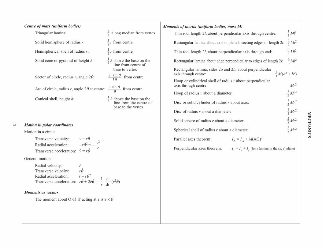
Centre of mass (uniform bodies)
Triangular lamina: along median from vertex
Solid hemisphere of radius r: r from centre
Hemispherical shell of radius r: r from centre
Solid cone or pyramid of height h: h above the base on the line from centre of base to vertex
Sector of circle, radius r, angle 2θ: from centre
Arc of circle, radius r, angle 2θ at centre: from centre
Conical shell, height h: h above the base on theline from the centre ofbase to the vertex
Motion in polar coordinates
Motion in a circle
Transverse velocity: v = rθRadial acceleration: –rθ2 = –
Transverse acceleration: v = rθ
General motion
Radial velocity: r
Transverse velocity: rθRadial acceleration: r – rθ2
Transverse acceleration: rθ + 2rθ = (r2θ)
Moments as vectors
The moment about O of F acting at r is r × F
d––dt
1–r
v2––r
1–3
r sin θ–––––––
θ
2r sin θ–––––––
3θ
1–4
1–2
3–8
2–3
Moments of inertia (uniform bodies, mass M)
Thin rod, length 2l, about perpendicular axis through centre: Ml2
Rectangular lamina about axis in plane bisecting edges of length 2l: Ml2
Thin rod, length 2l, about perpendicular axis through end: Ml2
Rectangular lamina about edge perpendicular to edges of length 2l: Ml2
Rectangular lamina, sides 2a and 2b, about perpendicularaxis through centre: M(a2 + b2)
Hoop or cylindrical shell of radius r about perpendicular axis through centre: Mr2
Hoop of radius r about a diameter: Mr2
Disc or solid cylinder of radius r about axis: Mr2
Disc of radius r about a diameter: Mr2
Solid sphere of radius r about a diameter: Mr2
Spherical shell of radius r about a diameter: Mr2
Parallel axes theorem: IA
= IG
+ M(AG)2
Perpendicular axes theorem: Iz
= Ix
+ Iy
(for a lamina in the (x, y) plane)
2–3
2–5
1–4
1–2
1–2
1–3
4–3
4–3
1–3
1–3

6
ST
AT
IST
ICS
Probability P(A∪B) = P(A) + P(B) – P(A∩B)
P(A∩B) = P(A) . P(B|A)
P(A|B) =
Bayes’ Theorem: P(Aj|B) =
Populations
Discrete distributions
X is a random variable taking values xiin a discrete distribution with
P(X = xi) = p
i
Expectation: µ = E(X) = ∑xip
i
Variance: σ2 = Var(X) = ∑(xi– µ)2 p
i= ∑x
i2p
i– µ2
For a function g(X): E[g(X)] = ∑g(xi)p
i
Continuous distributions
X is a continuous variable with probability density function (p.d.f.) f(x)
Expectation: µ = E(X) = ∫ x f(x)dx
Variance: σ2 = Var (X)
= ∫(x – µ)2 f(x)dx = ∫x2 f(x)dx – µ2
For a function g(X): E[g(X)] = ∫g(x)f(x)dx
Cumulative
distribution function F(x) = P(X < x) = ∫ x
–∞f(t)dt
Correlation and regression For a sample of n pairs of observations (xi, y
i)
Sxx
= ∑(xi– )2 = ∑x
i2 – , S
yy= ∑(y
i– )2 = ∑y
i2 – ,
Sxy
= ∑(xi– )(y
i– ) = ∑x
iy
i–
Covariance =∑ = ∑( – )( – )
–x x y y
n
x y
nx yi i i i
Sxy
––––n
(∑xi)(∑y
i)
–––––––––n
yx
(∑yi)2
–––––n
y(∑x
i)2
–––––n
x
P(Aj)P(B |A
j)
––––––––––––∑P(A
i)P(B|A
i)
P(B|A)P(A)––––––––––––––––––––––P(B|A)P(A) + P(B|A')P(A')
Product-moment correlation: Pearson’s coefficient
r = = =
Rank correlation: Spearman’s coefficient
rs
= 1 –
Regression
Least squares regression line of y on x: y – = b(x – )
b = = =
Estimates
Unbiased estimates from a single sample
for population mean µ; Var =
S2 for population variance σ2 where S2 = ∑(xi– )2f
i
Probability generating functions
For a discrete distribution
G(t) = E(tX)
E(X) = G'(1); Var(X) = G"(1) + µ – µ2
GX + Y
(t) = GX
(t) GY
(t) for independent X, Y
Moment generating functions:
MX(θ) = E(eθX)
E(X) = M'(0) = µ; E(Xn) = M(n)(0)
Var(X) = M"(0) – {M'(0)}2
MX + Y
(θ) = MX
(θ) MY(θ) for independent X, Y
x1––––n – 1
σ2––nXX
∑(xi– ) (y
i– )
–––––––––––––––∑(x
i– )2
Sxy
–––S
xx
xy
6∑di2
––––––––n(n2 – 1)
Σ
Σ Σ
x x y y
x x y y
i i
i i
– –
– –
( )( )( ) ( )[ ]2 2
S
S S
xy
xx yy
x
x
y∑
∑
x y
nx y
x
nx
i i
i
–
–2
2
∑
∑ −
∑ −
x y
nx y
x
nx
y
ny
i i
i i
–
2
2
2
2
7
ST
AT
IST
ICS
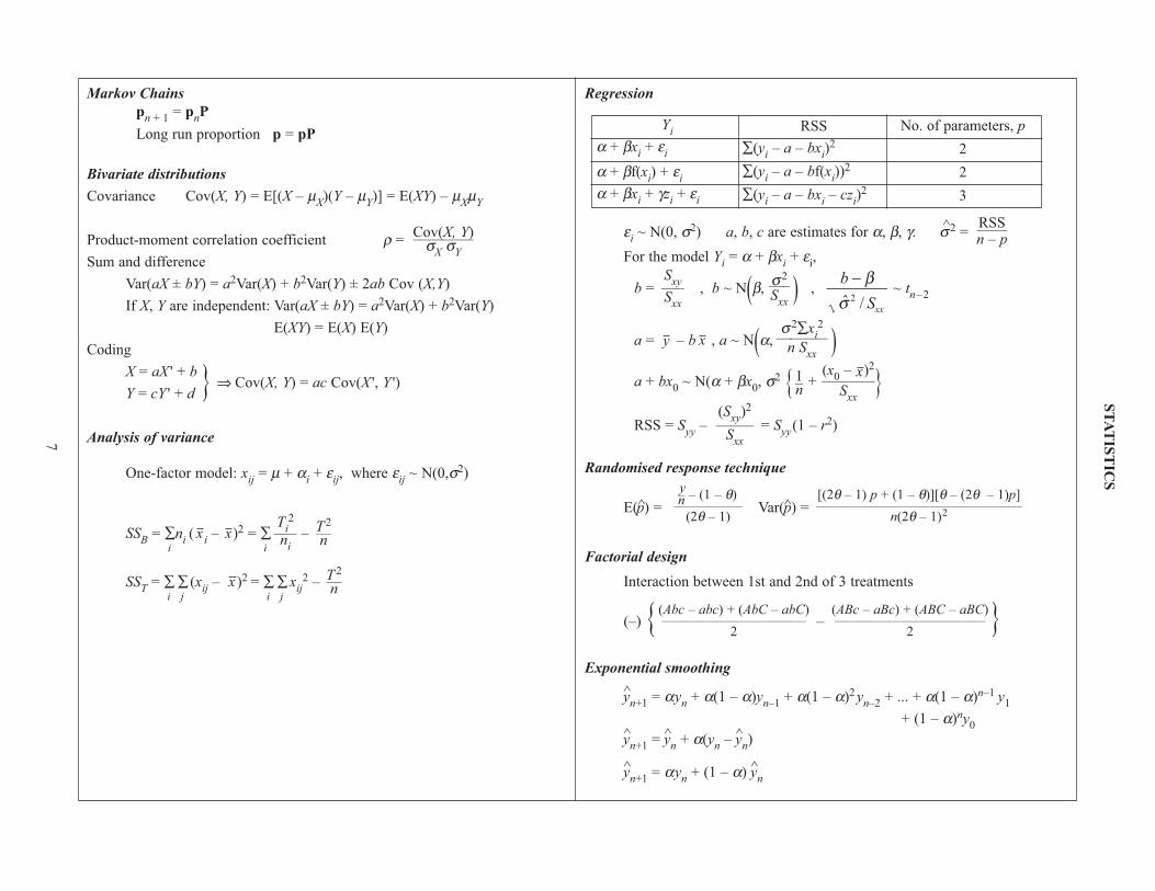
Markov Chains
pn + 1
= pnP
Long run proportion p = pP
Bivariate distributions
Covariance Cov(X, Y) = E[(X – µX)(Y – µ
Y)] = E(XY) – µ
Xµ
Y
Product-moment correlation coefficient ρ =
Sum and difference
Var(aX ± bY) = a2Var(X) + b2Var(Y) ± 2ab Cov (X,Y)
If X, Y are independent: Var(aX ± bY) = a2Var(X) + b2Var(Y)
E(XY) = E(X) E(Y)
Coding
X = aX ' + b } ⇒ Cov(X, Y) = ac Cov(X ', Y ')Y = cY ' + d
Analysis of variance
One-factor model: xij
= µ + αi+ ε
ij, where ε
ij~ N(0,σ2)
SSB
= ∑i
ni(
i– )2 = ∑
i
–
SST
= ∑i
∑j
(xij
– )2 = ∑i
∑j
xij
2 –T2––n
x
T2––n
Ti2
–––ni
xx
Cov(X, Y)––––––––σX
σY
Regression
εi~ N(0, σ2) a, b, c are estimates for α, β, γ. σ2 =
For the model Yi= α + βx
i+ ε
i,
b = , b ~ N(β, ) , ~ tn–2
a = – b , a ~ N(α, )a + bx
0~ N(α + βx
0, σ2 { + }
RSS = Syy
– = Syy
(1 – r2)
Randomised response technique
E(p) = Var(p) =
Factorial design
Interaction between 1st and 2nd of 3 treatments
(–) { – }
Exponential smoothing
yn+1
= αyn
+ α(1 – α)yn–1
+ α(1 – α)2 yn–2
+ ... + α(1 – α)n–1 y1
+ (1 – α)ny0
yn+1
= yn
+ α(yn
– yn)
yn+1
= αyn
+ (1 – α) yn
(ABc – aBc) + (ABC – aBC)––––––––––––––––––––––
2
(Abc – abc) + (AbC – abC)–––––––––––––––––––––
2
[(2θ – 1) p + (1 – θ)][θ – (2θ – 1)p]––––––––––––––––––––––––––––––
n(2θ – 1)2
y–n – (1 – θ)
––––––––––(2θ – 1)
1–n
σ2∑xi2
–––––––n S
xxxy
b
Sxx
− βσ /2
σ2–––S
xx
Sxy
–––S
xx
RSS––––n – p
Yi
α + βxi+ ε
i
α + βf(xi) + ε
i
α + βxi+ γz
i+ ε
i
RSS
∑(yi– a – bx
i)2
∑(yi– a – bf(x
i))2
∑(yi– a – bx
i– cz
i)2
No. of parameters, p
2
2
3
(x0
– )2
–––––––S
xx
x
(Sxy
)2
–––––S
xx
8
ST
AT
IST
ICS
: HY
PO
TH
ES
IS T
ES
TS
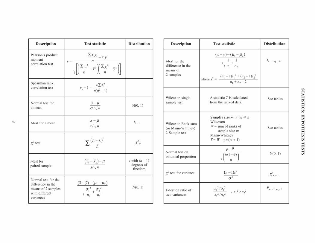
Description
Pearson’s product
moment
correlation test
Spearman rank
correlation test
Normal test for
a mean
t-test for a mean
χ2 test
Normal test for the
difference in the
means of 2 samples
with different
variances
Test statistic Distribution
r =
rs = 1 –
Description Test statistic Distribution
∑
∑
∑
x y
nx y
x
nx
y
ny
i i
i i
–
– –2
2
2
2
6∑di2
–––––––n(n2 – 1)
x
n
–
/
µσ
x
s n
–
/
µ
f f
f
o e
e
–( )∑2
(n1 – 1)s12 + (n2 – 1)s2
2
–––––––––––––––––––––––n1 + n2 – 2
( – ) – ( – )x y
sn n
µ µ1 2
1 2
1 1+
( – ) – ( – )x y
n n
µ µσ σ
1 2
12
1
22
2
+
N(0, 1)
N(0, 1)
tn1 + n2 – 2
tn –1
χ2v
See tables
See tables
χ2n – 1
N(0, 1)
Wilcoxon single
sample test
Wilcoxon Rank-sum
(or Mann-Whitney)
2-Sample test
Normal test on
binomial proportion
χ2 test for variance
F-test on ratio of
two variances
A statistic T is calculated
from the ranked data.
Samples size m, n: m < n
Wilcoxon
W = sum of ranks of
sample size m
Mann-Whitney
T = W – m(m + 1)
p
n
–
( – )
θθ θ1
n s–1 2
2
( )σ
1–2
Fn1–1, n
2–1
t-test for
paired sample
t with (n – 1) degrees offreedom
x x
s
1 2– –( ) µ/ n
t-test for the
difference in the
means of
2 samples
where s2 =
s12 /σ1
2
–––––––s2
2 /σ22
, s12 > s2
2
9
ST
AT
IST
ICS
: DIS
TR
IBU
TIO
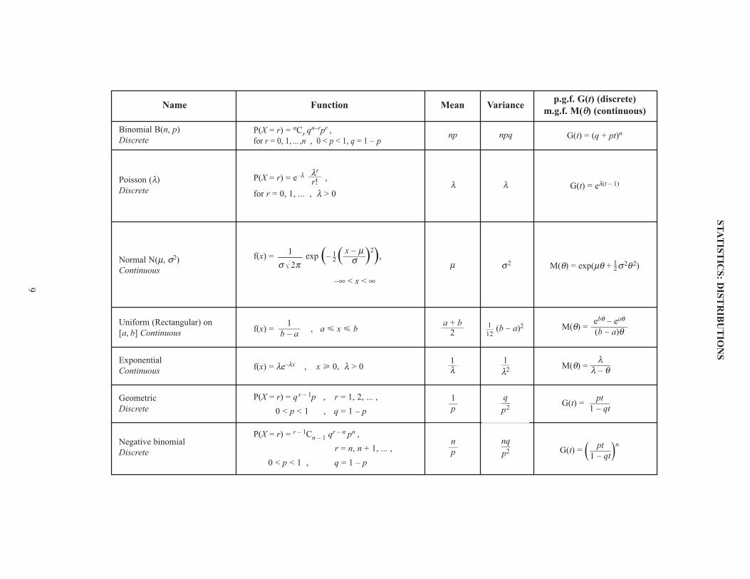
NS
Name
Binomial B(n, p)
Discrete
Poisson (λ)
Discrete
Normal N(µ, σ2)
Continuous
Uniform (Rectangular) on
[a, b] Continuous
Exponential
Continuous
Geometric
Discrete
Negative binomial
Discrete
Function
P(X = r) = nCr qn–rpr ,
for r = 0, 1, ... ,n , 0 < p < 1, q = 1 – p
P(X = r) = e–λ ,
for r = 0, 1, ... , λ > 0
f(x) = exp (–W( )2),
–∞ < x < ∞
f(x) = , a < x < b
f(x) = λe–λx , x > 0, λ > 0
P(X = r) = q r – 1p , r = 1, 2, ... ,
0 < p < 1 , q = 1 – p
P(X = r) = r – 1Cn – 1 qr – n pn ,
r = n, n + 1, ... ,
0 < p < 1 , q = 1 – p
Mean Variance
λ
µ
(b – a)2a + b–––––
2
1––λ
1––λ2
λ
σ2
p.g.f. G(t) (discrete)
m.g.f. M(θ) (continuous)
G(t) = (q + pt)n
G(t) = eλ(t – 1)
M(θ) = exp(µθ + Wσ2θ2)
M(θ) =
G(t) = ( )n
G(t) =
M(θ) =
nq––p2
n––p
1––p
q––p2
np npq
λr–––r!
pt–––––1 – qt
pt–––––1 – qt
λ–––––λ – θ
ebθ – eaθ–––––––––(b – a)θ
1
2σ πx – µ–––––σ
1––12
1–––––b – a
10
NU
ME
RIC
AL
AN
AL
YS
IS
DE
CIS
ION
& D
ISC
RE
TE
MA
TH
EM
AT
ICS
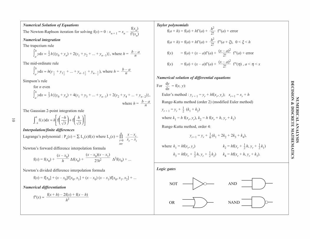
Numerical Solution of Equations
The Newton-Raphson iteration for solving f(x) = 0 : xn + 1
= xn
–
Numerical integration
The trapezium rule
∫b
aydx ≈ h{(y
0+ y
n) + 2(y
1+ y
2+ ... + y
n–1)}, where h =
The mid-ordinate rule
∫b
aydx ≈ h(y + y
1+ ... + y
n–1+ y
n–), where h =
Simpson’s rule
for n even
∫b
aydx ≈ h{(y
0+ y
n) + 4(y
1+ y
3+ ... + y
n–1) + 2(y
2+ y
4+ ... + y
n–2)},
where h =
The Gaussian 2-point integration rule
Interpolation/finite differences
Lagrange’s polynomial : Pn(x) = ∑ L
r(x)f(x) where L
r(x) = ∏
n
i=0i≠r
Newton’s forward difference interpolation formula
f(x) = f(x0) + ∆f(x
0) + ∆2f(x
0) + ...
Newton’s divided difference interpolation formula
f(x) = f[x0] + (x – x
0]f[x
0, x
1] + (x – x
0) (x – x
1)f[x
0, x
1, x
2] + ...
Numerical differentiation
f"(x) ≈ f(x + h) – 2f(x) + f(x – h)–––––––––––––––––––––
h2
(x – x0)(x – x
1)
––––––––––––2!h2
(x – x0)
––––––h
x – xi––––––
xr
– xi
b – a–––––n
1–3
b – a–––––n1–2
1–2
1–2
1–2
b – a–––––n1–2
f(xn)
––––f '(x
n)
Taylor polynomials
f(a + h) = f(a) + hf '(a) + f"(a) + error
f(a + h) = f(a) + hf '(a) + f"(a + ξ), 0 < ξ < h
f(x) = f(a) + (x – a)f '(a) + f"(a) + error
f(x) = f(a) + (x – a)f '(a) + f"(η) , a < η < x
Numerical solution of differential equations
For = f(x, y):
Euler’s method : yr + 1
= yr
+ hf(xr, y
r); x
r+1= x
r+ h
Runge-Kutta method (order 2) (modified Euler method)
yr + 1
= yr
+ (k1
+ k2)
where k1
= h f(xr, y
r), k
2= h f(x
r+ h, y
r+ k
1)
Runge-Kutta method, order 4:
yr+1
= yr
+ (k1
+ 2k2
+ 2k3
+ k4),
where k1
= hf(xr, y
r) k
2= hf(x
r+ h, y
r+ k
1)
k3
= hf(xr
+ h, yr
+ k2) k
4= hf(x
r+ h, y
r+ k
3).
Logic gates
1–2
1–2
1–2
1–2
1–6
1–2
dy––dx
(x – a)2––––––
2!
(x – a)2––––––
2!
h2–––2!
h2–––2!
f d( )–
x x hh h
h
h
≈ −
+
∫ f f
3 3
NOT
OR
AND
NAND
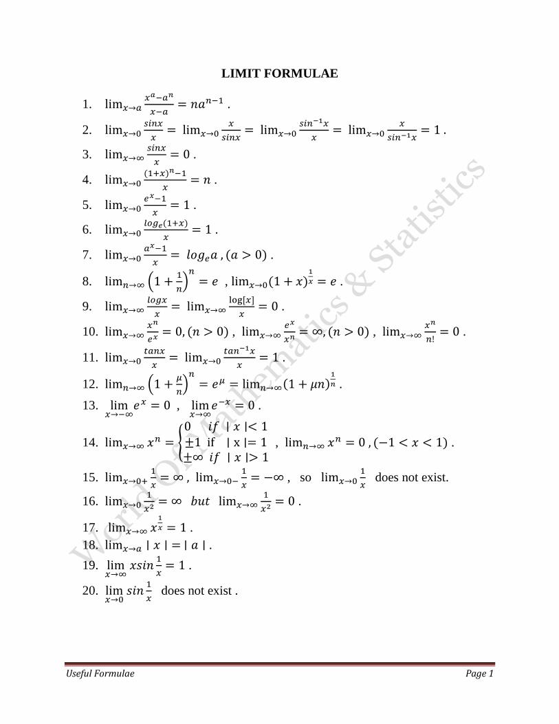
Useful Formulae Page 1
LIMIT FORMULAE
1.
.
2.
3.
.
4.
.
5.
.
6.
.
7.
.
8. (
)
,
.
9.
.
10.
,
,
.
11.
.
12. (
)
.
13.
,
.
14. {
, .
15.
, so
does not exist.
16.
.
17.
.
18. .
19.
.
20.
does not exist .
Useful Formulae Page 2
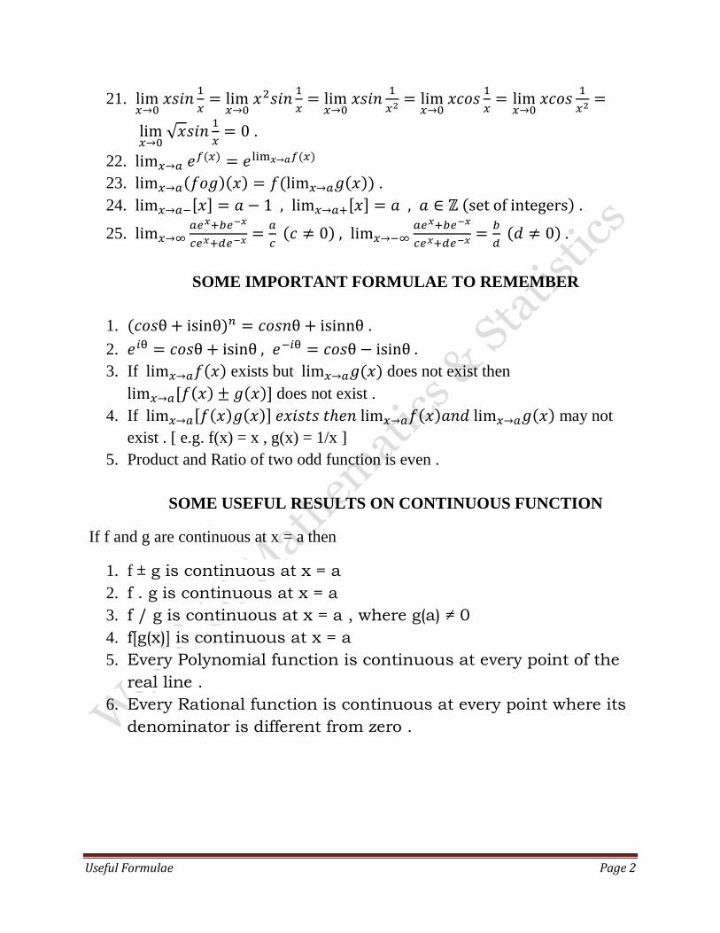
21.
√
.
22.
23. .
24. .
25.
.
SOME IMPORTANT FORMULAE TO REMEMBER
1. .
2.
3. If exists but does not exist then
does not exist .
4. If may not
exist . [ e.g. f(x) = x , g(x) = 1/x ]
5. Product and Ratio of two odd function is even .
SOME USEFUL RESULTS ON CONTINUOUS FUNCTION
If f and g are continuous at x = a then
1. f ± g is continuous at x = a
2. f . g is continuous at x = a
3. f / g is continuous at x = a , where g(a) ≠ 0
4. f[g(x)] is continuous at x = a
5. Every Polynomial function is continuous at every point of the
real line .
6. Every Rational function is continuous at every point where its
denominator is different from zero .
Useful Formulae Page 3
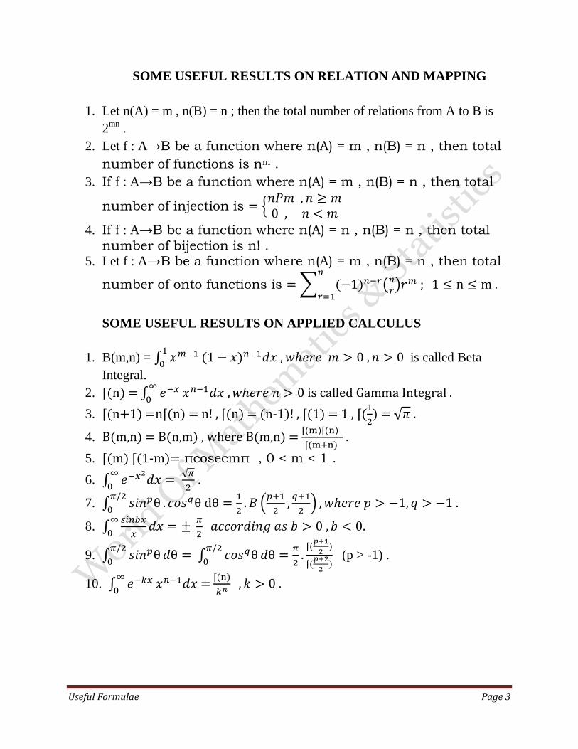
SOME USEFUL RESULTS ON RELATION AND MAPPING
1. Let n(A) = m , n(B) = n ; then the total number of relations from A to B is
2mn
.
2. Let f : A→B be a function where n(A) = m , n(B) = n , then total
number of functions is nm .
3. If f : A→B be a function where n(A) = m , n(B) = n , then total
number of injection is {
4. If f : A→B be a function where n(A) = n , n(B) = n , then total
number of bijection is n! . 5. Let f : A→B be a function where n(A) = m , n(B) = n , then total
number of onto functions is ∑ ( )
SOME USEFUL RESULTS ON APPLIED CALCULUS
1. B(m,n) = ∫
is called Beta
Integral.
2. ⌈(n) = ∫
is called Gamma Integral .
3. ⌈(n+1) =n⌈(n) = n! , ⌈(n) = (n-1)! , ⌈(1) = 1 , ⌈(
) = √ .
4. B(m,n) = B(n,m) , where B(m,n) = ⌈ ⌈
⌈ .
5. ⌈(m) ⌈(1-m)= πcosecmπ , 0 < m < 1 .
6. ∫
√
.
7. ∫
(
)
8. ∫
9. ∫
∫
⌈
⌈
(p > -1) .
10. ∫
=
⌈
Useful Formulae Page 4
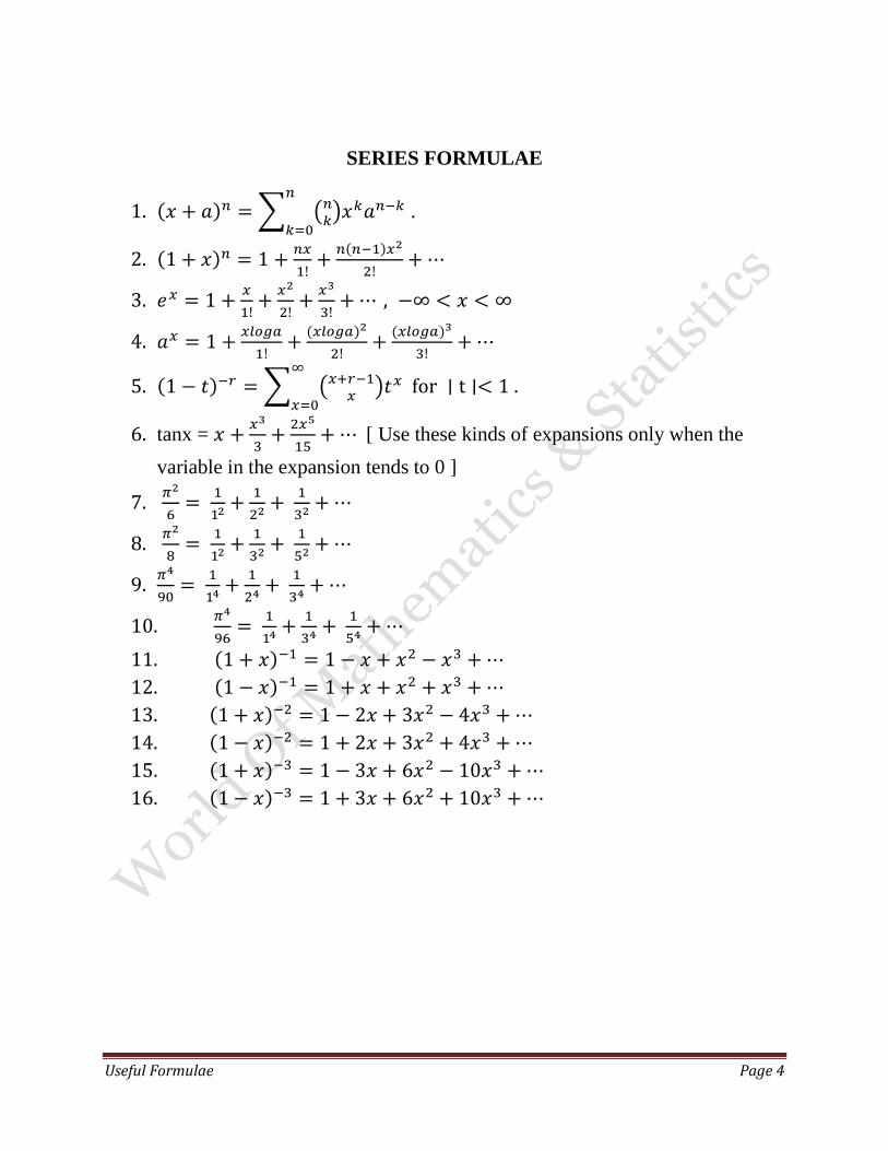
SERIES FORMULAE
1. ∑ ( )
.
2.
3.
4.
5. ∑ (
)
6. tanx =
[ Use these kinds of expansions only when the
variable in the expansion tends to 0 ]
7.
8.
9.
10.
11.
12.
13.
14.
15.
16.
1
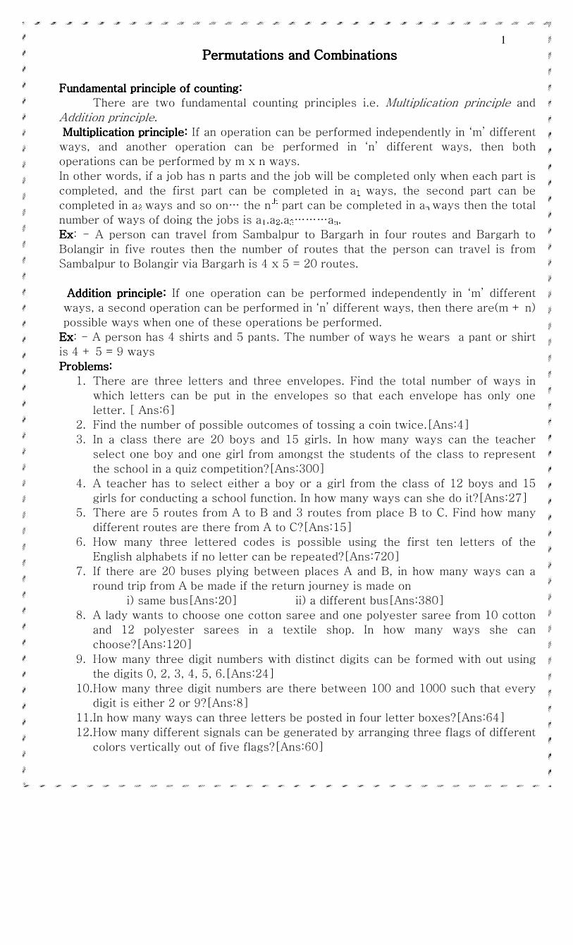
Permutations and CombinationsPermutations and CombinationsPermutations and CombinationsPermutations and Combinations
Fundamental principle of counting:Fundamental principle of counting:Fundamental principle of counting:Fundamental principle of counting:
There are two fundamental counting principles i.e. Multiplication principle and
Addition principle.
Multiplication principle:Multiplication principle:Multiplication principle:Multiplication principle: If an operation can be performed independently in ‘m’ different
ways, and another operation can be performed in ‘n’ different ways, then both
operations can be performed by m x n ways.
In other words, if a job has n parts and the job will be completed only when each part is
completed, and the first part can be completed in a1 ways, the second part can be
completed in a2 ways and so on… the nth part can be completed in an ways then the total
number of ways of doing the jobs is a1.a2.a3………an. ExExExEx: - A person can travel from Sambalpur to Bargarh in four routes and Bargarh to
Bolangir in five routes then the number of routes that the person can travel is from
Sambalpur to Bolangir via Bargarh is 4 x 5 = 20 routes.
Addition principle:Addition principle:Addition principle:Addition principle: If one operation can be performed independently in ‘m’ different
ways, a second operation can be performed in ‘n’ different ways, then there are(m + n)
possible ways when one of these operations be performed.
ExExExEx: - A person has 4 shirts and 5 pants. The number of ways he wears a pant or shirt
is 4 + 5 = 9 ways
Problems:Problems:Problems:Problems:
1. There are three letters and three envelopes. Find the total number of ways in
which letters can be put in the envelopes so that each envelope has only one
letter. [ Ans:6]
2. Find the number of possible outcomes of tossing a coin twice.[Ans:4]
3. In a class there are 20 boys and 15 girls. In how many ways can the teacher
select one boy and one girl from amongst the students of the class to represent
the school in a quiz competition?[Ans:300]
4. A teacher has to select either a boy or a girl from the class of 12 boys and 15
girls for conducting a school function. In how many ways can she do it?[Ans:27]
5. There are 5 routes from A to B and 3 routes from place B to C. Find how many
different routes are there from A to C?[Ans:15]
6. How many three lettered codes is possible using the first ten letters of the
English alphabets if no letter can be repeated?[Ans:720]
7. If there are 20 buses plying between places A and B, in how many ways can a
round trip from A be made if the return journey is made on
i) same bus[Ans:20] ii) a different bus[Ans:380]
8. A lady wants to choose one cotton saree and one polyester saree from 10 cotton
and 12 polyester sarees in a textile shop. In how many ways she can
choose?[Ans:120]
9. How many three digit numbers with distinct digits can be formed with out using
the digits 0, 2, 3, 4, 5, 6.[Ans:24]
10. How many three digit numbers are there between 100 and 1000 such that every
digit is either 2 or 9?[Ans:8]
11. In how many ways can three letters be posted in four letter boxes?[Ans:64]
12. How many different signals can be generated by arranging three flags of different
colors vertically out of five flags?[Ans:60]
2
13. In how many ways can three people be seated in a row containing seven
seats?[Ans:210]
14. There are five colleges in a city. In how many ways can a man send three of his
children to a college if no two of the children are to read in the same
college?[Ans:60]
15. How many even numbers consisting of 4 digits can be formed by using the digits
1, 2, 3, 5, 7?[Ans:24]
16. How many four digit numbers can be formed with the digits 4,3,2,0 digits not
being repeated?[Ans:18]
17. How many different words with two letters can be formed by using the letters of
the word JUNGLE, each containing one vowel and one consonant?[Ans:16]
18. How many numbers between 99 and 1000 can be formed with the digits 0, 1, 2, 3,
4 and 5?[Ans:180]
19. There are three multiple choice questions in an examination. How many
sequences of answers are possible, if each question has two choices?[Ans:8]
20. There are four doors leading to the inside of a cinema hall. In how many ways
can a person enter into it and come out?[Ans:16]
21. Find the number of possible outcomes if a die is thrown 3 times.[Ans:216]
22. How many three digit numbers can be formed from the digits 1,2,3,4, and 5, if the
repetition of the digits is not allowed.[Ans:60]
23. How many numbers can be formed from the digits 1,2,3, and 9 , if the repetition
of the digits is not allowed.[Ans:24]
24. How many four digit numbers greater than 2300 can be formed with the digits
0,1,2,3,4,5 and 6, no digit being repeated in any number.[Ans:560]
25. How many two digit even numbers can be formed from the digits 1,2,3,4,5 if the
digits can be repeated?[Ans:10]
26. How many three digits numbers have exactly one of the digits as 5 if repetition is
not allowed?[Ans:200]
27. How many 5 digit telephone numbers can be constructed using the digits 0 to 9 if
each number starts with 59 and no digit appears more than once.[Ans:210]
28. In how many ways can four different balls be distributed among 5 boxes, when
i) no box has more than one ball[Ans:120]
ii) a box can have any number of balls[Ans:625]
29. Rajeev has 3 pants and 2 shirts. How many different pairs of a pant and a shirt,
can he dress up with?[Ans:6]
30. Ali has 2 school bags, 3 tiffin boxes and 2 water bottles. In how many ways can
he carry these items choosing one each?[Ans:12]
31. How many three digit numbers with distinct digits are there whose all the digits
are odd?[Ans:60]
32. A team consists of 7 boys and 3 girls plays singles matches against another team
consisting of 5 boys and 5 girls. How many matches can be scheduled between
the two teams if a boy plays against a boy and a girl plays against a girl.[Ans:50]
33. How many non- zero numbers can be formed using the digits 0, 1, 2, 3, 4, 5 if
repetition of the digits is not allowed? [Ans:600]
34. In how many ways can five people be seated in a car with two people in the front
seat including driver and three in the rear, if two particular persons out of the
five can not drive?[Ans:72]
35. How many A.P’s with 10 terms are there whose first term belongs to the
set{1,2,3} and common difference belongs to the set {1,2,3,4,5}[Ans:15]
3
FactorialFactorialFactorialFactorial: The product of first n natural numbers is generally written as n! or n∠ and is
read factorial n.
Thus, n! = 1. 2. 3.………..n.
ExExExEx: 123456!6 ×××××= =720
Note:Note:Note:Note:
1) 0! =1
2) (-r)! = ∞
Problems:Problems:Problems:Problems:
1. Evaluate the following:
i) 7! ii) 5! iii) 8! iv) 8!-5! v) 4!-3! vii) 7!-5! viii)!5
!6
ix) !5
!7 x)
!2!6
!8 xi)
!2!10
!12 xii) (3!)(5!) xiii)
!5
1+
!6
1+
!7
1 xiv)
2!3! 2. Evaluate
)!(!
!
rnr
n
−, when
i) n=7, r=3 ii) n=15, r=12 iii) n=5, r=2
3. Evaluate )!(
!
rn
n
−, when
i) n=9, r=5 ii) n=6, r=2
4. Convert the following into factorials:
i) 1.3.5.7.9.11 ii) 2.4.6.8.10 iii) 5.6.7.8.9 iv)
(n+1)(n+2)(n+3)…………2n
5. Find x if
i) !5
1+
!6
1=
!7
x ii)
!8
1+
!9
1=
!10
x
6. Find the value of n if
i) (n+1)!=12(n-1)! ii) (2n)!n!=(n+1)(n-1)!(2n-1)!
7. If )!2(!2
!
−n
n and
)!4(!4
!
−n
n are in the ratio 2:1 find the value of n.
8. Find the value of x if)!12(
)!2(
−
+
x
x.
)!3(
)!12(
+
+
x
x=
7
72 where Nx ∈
9. Show that n!(n+2)=n!+(n+1)!
10. Show that 27! Is divisible by 122 . What is the largest natural number n such that
27! is divisible by 2n. 11. Show that 24! +1 is not divisible by any number between 2 to 24.
12. Prove that (n!)2 ≤ nn n! < (2n)!
13. Find the value of x if)!1(
)!32(
+
+
x
x.
)!12(
)!1(
+
−
x
x=7
14. Prove that the product of k consecutive positive integers is divisible by k! for
2≥k
15. Show that 2.6.10……..to n factors =!
)!2(
n
n.
4
PermutationPermutationPermutationPermutation:- The different arrangements which can be made by taking some or all at a
time from a number of objects are called permutations. In forming permutations we are
concerned with the order of the things. For example the arrangements which can be
made by taking the letters a, b, c two at a time are six numbers, namely,
ab , bc, ca, ba, cb, ac
Thus the permutations of 3 things taken two at a time are 6.
a) Without repetitiona) Without repetitiona) Without repetitiona) Without repetition:
i) If there are n distinct objects then the number of permutations of n objects taking r
at a time with out repetition is denoted by npr or p (n ,r) and is defined as , nr ≤≤0
ProofProofProofProof: Arrangements of n objects, taken r at a time, is same to filling r places with n
things
1st place can be filled up in n ways
2nd place can be filled up in n-1 ways
3rd place can be filled up in n-2 ways
……………………………………….
……………………………………….
rth place can be filled up in n-(r-1) ways
∴the number of arrangements
r
n p = ))1(........().........2)(1( −−−− rnnnn
= )!(
)!)(1.......().........2)(1(
rn
rnrnnnn
−
−+−−−
r
n p =)!(
!
rn
n
−.
ii) Number of arrangements of n different things taken all at a time without repetition
= !)!(
!n
nn
npn
n =−
=
b) With repetitionb) With repetitionb) With repetitionb) With repetition:
i) If there are n distinct objects then the number of permutations of n objects
taking r at a time with repetition is nr. ii) Number of arrangements of n different things taken all at a time with repetition
is nn. c) If p objects of one kind, q objects of second kind are there then the total number of
permutations of all the
p + q objects are given by!!
)!(
qp
qp +.
In general If ai objects of ith kind, i= 1, 2, 3…..,r are there then the number of
permutations of all the a1+a2+……….+ar objects is given by !..!.........!
)!.........(
21
321
r
r
aaa
aaaa ++++.
)!(
!
rn
npr
n
−=
5
d) Circular arrangementsd) Circular arrangementsd) Circular arrangementsd) Circular arrangements:
i) The number of circular arrangements of n distinct objects taking all at a time is
(n-1)!
ii) The number of circular arrangements of n distinct objects when clockwise and
anti-clockwise circular permutations are considered as same is2
)!1( −n.
iii) The number of circular permutations of n different things taken r at a time is
r
pr
n
( if clockwise and anti-clockwise circular permutations are considered as different)
Ex:Ex:Ex:Ex: The number of which 29 persons be seated in a round table if there are 9 chairs
is 9
9
29p
iv) The number of circular permutations of n different things taken r at a time is
r
pr
n
2( if clockwise and anti-clockwise circular permutations are considered as same).
Restricted permutations:Restricted permutations:Restricted permutations:Restricted permutations:
1)1)1)1) The number of permutations of n dissimilar things taken r at a time when one
particular thing always occurs is r n-1Pr-1 2)2)2)2) The number of permutations of n dissimilar things taken r at a time when one
particular thing taken is
n-1Pr. 3) The number of permutations of n dissimilar things taken r at a time when p
particular things always occurs = !.rC pr
pn
−
−
4) The number of permutations of n dissimilar things taken r at a time when p
particular things never occurs !.rCr
pn−
Zero Factorial:Zero Factorial:Zero Factorial:Zero Factorial:
The value of Zero factorial is 1 i.e. 0! =1
Proof: Proof: Proof: Proof:
By the fundamental principle of counting we know that the number of
permutations of n different objects taken all at a time with out repetition is
!1.2.3.).........2)(1( nnnn =−− ………(1)
And we have seen )!(
!
rn
npr
n
−= …………… (2)
From (2) the number of permutations of n different objects taken all at a time with out
repetition is
!0
!
)!(
! n
nn
npn
n =−
= ……………… (3)
from (1) and (3) !0
!!
nn =
and this can be hold true if 0! is 1.
1!0 =∴
6
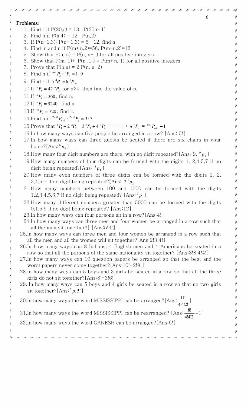
Problems:Problems:Problems:Problems:
1. Find r if P(20,r) = 13. P(20,r-1)
2. Find n if P(n,4) = 12. P(n,2)
3. If P(n-1,3): P(n+1,3) = 5 : 12, find n
4. Find m and n if P(m+n,2)=56, P(m-n,2)=12
5. Show that P(n, n) = P(n, n-1) for all positive integers.
6. Show that P(m, 1)+ P(n ,1 ) = P(m+n, 1) for all positive integers
7. Prove that P(n,n) = 2 P(n, n-2)
8. Find n if 9:1: 43
1 =−PP
nn
9. Find r if 1
54 65 −= rr PP
10. If ,42 35 PPnn = for n>4, then find the value of n.
11. If 3604 =Pn , find n.
12. If 92403 =Pn , find n.
13. If 72010 =rP , find r.
14. Find n if 5:3: 12
1
12 =−
−
+
n
n
n
nPP
15. Prove that 2
2
1
1 2 PP + + 4
4
3
3 43 PP + +………+ n
nPn = 11
1 −+
+
n
nP
16. In how many ways can five people be arranged in a row? [Ans: 5!]
17. In how many ways can three guests be seated if there are six chairs in your
home?[Ans: 3
6p ]
18. How many four digit numbers are there, with no digit repeated?[Ans: 9. 3
9p ]
19. How many numbers of four digits can be formed with the digits 1, 2,4,5,7 if no
digit being repeated?[Ans: 4
5 p ]
20. How many even numbers of three digits can be formed with the digits 1, 2,
3,4,5,7 if no digit being repeated?[Ans: 2
5.2 p
21. How many numbers between 100 and 1000 can be formed with the digits
1,2,3,4,5,6,7 if no digit being repeated? [Ans: 3
7p ]
22. How many different numbers greater than 5000 can be formed with the digits
0,1,5,9 if no digit being repeated? [Ans:12]
23. In how many ways can four persons sit in a row?[Ans:4!]
24. In how many ways can three men and four women be arranged in a row such that
all the men sit together?[ [Ans:5!3!]
25. In how many ways can three men and four women be arranged in a row such that
all the men and all the women will sit together?[Ans:2!3!4!]
26. In how many ways can 8 Indians, 4 English men and 4 Americans be seated in a
row so that all the persons of the same nationality sit together? [Ans:3!8!4!4!]
27. In how many ways can 10 question papers be arranged so that the best and the
worst papers never come together?[Ans:10!-2!9!]
28. In how many ways can 5 boys and 3 girls be seated in a row so that all the three
girls do not sit together?[Ans:8!-3!6!]
29. In how many ways can 5 boys and 4 girls be seated in a row so that no two girls
sit together?[Ans: !54
7 p ]
30. In how many ways the word MISSISSIPPI can be arranged?[Ans:!2!4!4
!11]
31. In how many ways the word MISSISSIPPI can be rearranged? [Ans: 1!2!4!4
!8− ]
32. In how many ways the word GANESH can be arranged?[Ans:6!]
7
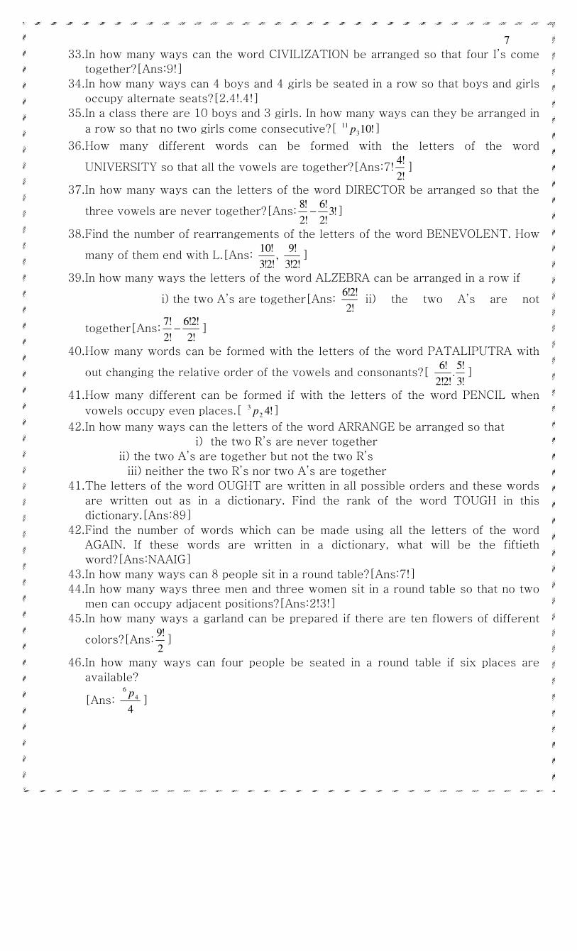
33. In how many ways can the word CIVILIZATION be arranged so that four I’s come
together?[Ans:9!]
34. In how many ways can 4 boys and 4 girls be seated in a row so that boys and girls
occupy alternate seats?[2.4!.4!]
35. In a class there are 10 boys and 3 girls. In how many ways can they be arranged in
a row so that no two girls come consecutive?[ !103
11p ]
36. How many different words can be formed with the letters of the word
UNIVERSITY so that all the vowels are together?[Ans:7!!2
!4]
37. In how many ways can the letters of the word DIRECTOR be arranged so that the
three vowels are never together?[Ans: !3!2
!6
!2
!8− ]
38. Find the number of rearrangements of the letters of the word BENEVOLENT. How
many of them end with L.[Ans: !2!3
!9,
!2!3
!10]
39. In how many ways the letters of the word ALZEBRA can be arranged in a row if
i) the two A’s are together[Ans: !2
!2!6 ii) the two A’s are not
together[Ans:!2
!2!6
!2
!7− ]
40. How many words can be formed with the letters of the word PATALIPUTRA with
out changing the relative order of the vowels and consonants?[ !3
!5.
!2!2
!6]
41. How many different can be formed if with the letters of the word PENCIL when
vowels occupy even places.[ !42
3 p ]
42. In how many ways can the letters of the word ARRANGE be arranged so that
i) the two R’s are never together
ii) the two A’s are together but not the two R’s
iii) neither the two R’s nor two A’s are together
41. The letters of the word OUGHT are written in all possible orders and these words
are written out as in a dictionary. Find the rank of the word TOUGH in this
dictionary.[Ans:89]
42. Find the number of words which can be made using all the letters of the word
AGAIN. If these words are written in a dictionary, what will be the fiftieth
word?[Ans:NAAIG]
43. In how many ways can 8 people sit in a round table?[Ans:7!]
44. In how many ways three men and three women sit in a round table so that no two
men can occupy adjacent positions?[Ans:2!3!]
45. In how many ways a garland can be prepared if there are ten flowers of different
colors?[Ans:2
!9]
46. In how many ways can four people be seated in a round table if six places are
available?
[Ans: 4
4
6 p]
8
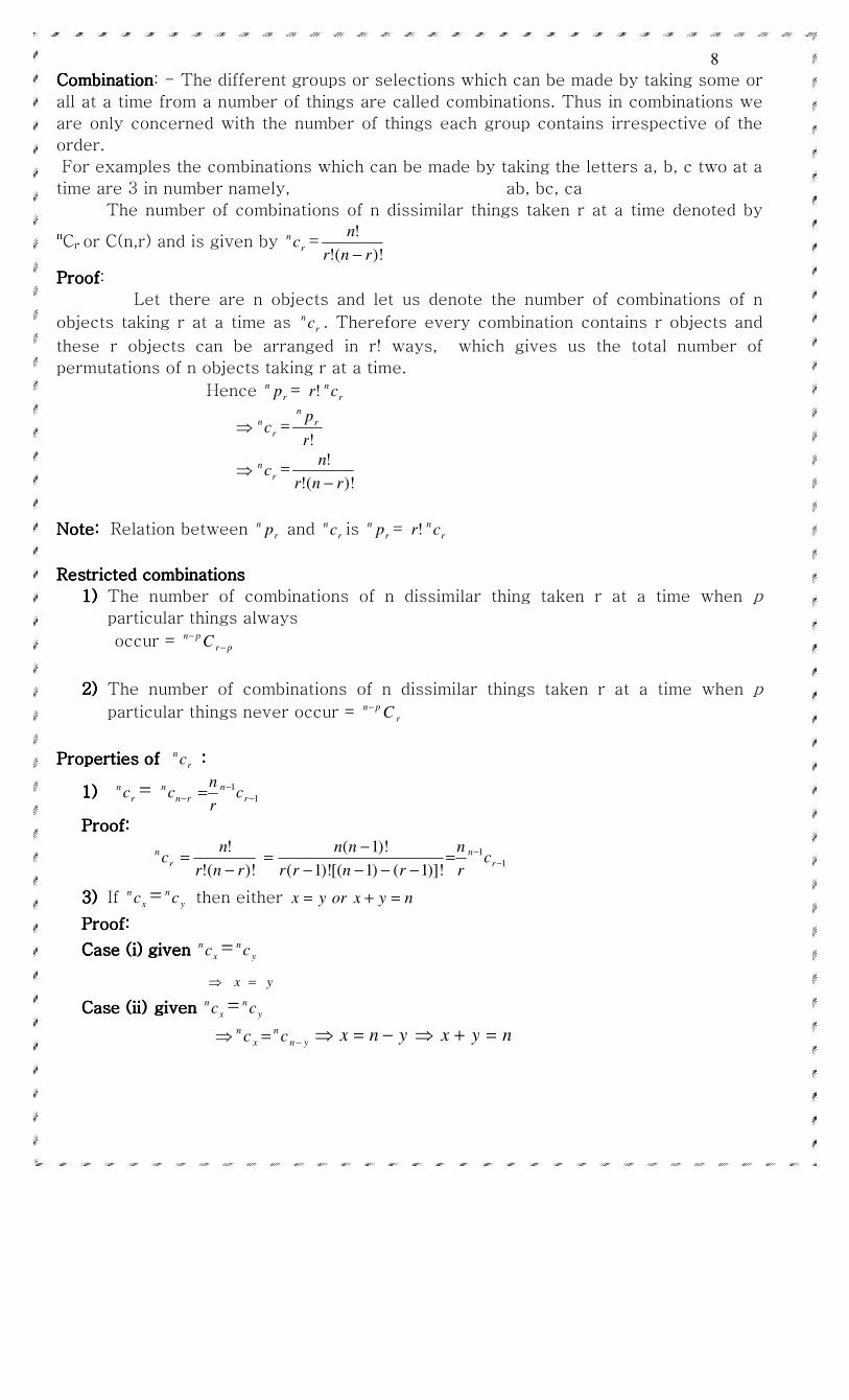
CombinationCombinationCombinationCombination: - The different groups or selections which can be made by taking some or
all at a time from a number of things are called combinations. Thus in combinations we
are only concerned with the number of things each group contains irrespective of the
order.
For examples the combinations which can be made by taking the letters a, b, c two at a
time are 3 in number namely, ab, bc, ca
The number of combinations of n dissimilar things taken r at a time denoted by nCr or C(n,r) and is given by r
nc =)!(!
!
rnr
n
−
ProofProofProofProof:
Let there are n objects and let us denote the number of combinations of n
objects taking r at a time as r
nc . Therefore every combination contains r objects and
these r objects can be arranged in r! ways, which gives us the total number of
permutations of n objects taking r at a time.
Hence r
n p = !r r
nc
⇒ r
nc =!r
pr
n
⇒ r
nc =)!(!
!
rnr
n
−
Note:Note:Note:Note: Relation between r
n p and r
nc is r
n p = !r r
nc
Restricted combinationsRestricted combinationsRestricted combinationsRestricted combinations
1)1)1)1) The number of combinations of n dissimilar thing taken r at a time when p
particular things always
occur = pr
pnC −
−
2)2)2)2) The number of combinations of n dissimilar things taken r at a time when p
particular things never occur = r
pn C−
Properties of Properties of Properties of Properties of r
nc ::::
1) 1) 1) 1) r
nc = 1
1
−
−
− = r
n
rn
nc
r
nc
Proof:Proof:Proof:Proof:
1
1
)]!1()1[()!1(
)!1(
)!(!
!−
−=−−−−
−=
−= r
n
r
n cr
n
rnrr
nn
rnr
nc
3)3)3)3) If x
nc = y
nc then either nyxoryx =+=
Proof:Proof:Proof:Proof:
Case (i) given Case (i) given Case (i) given Case (i) given x
nc = y
nc
yx =⇒
Case (ii)Case (ii)Case (ii)Case (ii) given given given given x
nc = y
nc
yn
n
x
ncc −=⇒ ynx −=⇒ nyx =+⇒
9
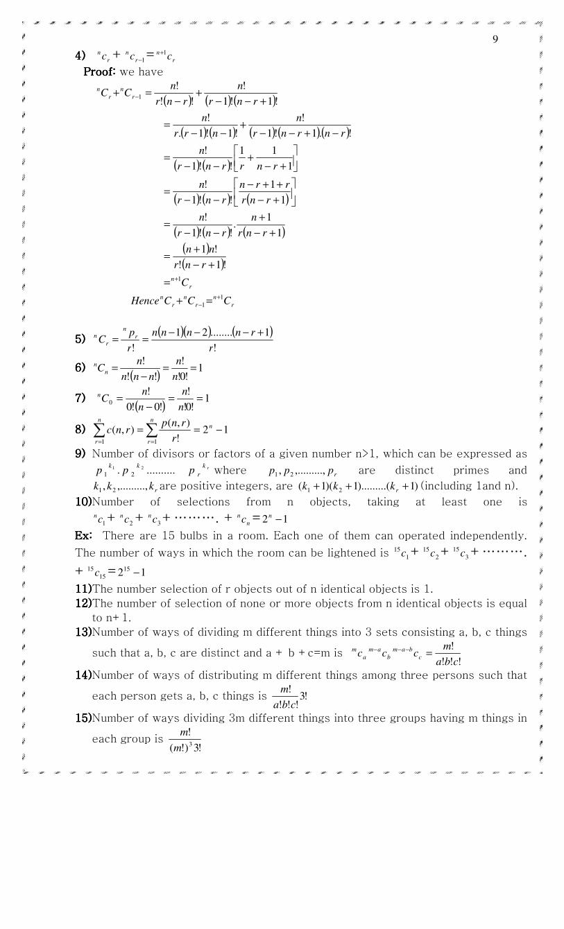
4)4)4)4) r
nc + 1−r
nc = r
n c1+
Proof: Proof: Proof: Proof: we have
( ) ( ) ( )
( ) ( ) ( ) ( )( )
( ) ( )
( ) ( ) ( )
( ) ( ) ( )( )( )
r
n
r
n
r
n
r
n
r
n
r
n
CCCHence
C
rnr
nn
rnr
n
rnr
n
rnr
rrn
rnr
n
rnrrnr
n
rnrnr
n
nrr
n
rnr
n
rnr
nCC
1
1
1
1
!1!
!1
1
1.
!!1
!
1
1
!!1
!
1
11
!!1
!
!.1!1
!
!1!1.
!
!1!1
!
!!
!
+
−
+
−
=+
=
+−
+=
+−
+
−−=
+−
++−
−−=
+−+
−−=
−+−−+
−−=
+−−+
−=+
5)5)5)5) ( )( ) ( )
!
1........21
! r
rnnnn
r
pC r
n
r
n +−−−==
6)6)6)6) ( )
1!0!
!
!!
!==
−=
n
n
nnn
nCn
n
7)7)7)7) ( )
1!0!
!
!0!0
!0 ==
−=
n
n
n
nCn
8)8)8)8) ∑∑==
−==n
r
nn
r r
rnprnc
11
12!
),(),(
9)9)9)9) Number of divisors or factors of a given number n>1, which can be expressed as rk
r
kkppp ........... 21
21 where rppp ,,........., 21 are distinct primes and
rkkk ,,........., 21 are positive integers, are )1().........1)(1( 21 +++ rkkk (including 1and n).
10)10)10)10) Number of selections from n objects, taking at least one is
1cn+ 2cn
+ 3cn
+………. + n
nc = 12 −n
Ex:Ex:Ex:Ex: There are 15 bulbs in a room. Each one of them can operated independently.
The number of ways in which the room can be lightened is 1
15c + 2
15c + 3
15c +……….
+ 15
15c = 1215 −
11)11)11)11) The number selection of r objects out of n identical objects is 1.
12)12)12)12) The number of selection of none or more objects from n identical objects is equal
to n+1.
13)13)13)13) Number of ways of dividing m different things into 3 sets consisting a, b, c things
such that a, b, c are distinct and a + b +c=m is !!!
!
cba
mccc c
bam
b
am
a
m =−−−
14)14)14)14) Number of ways of distributing m different things among three persons such that
each person gets a, b, c things is !3!!!
!
cba
m
15)15)15)15) Number of ways dividing 3m different things into three groups having m things in
each group is !3)!(
!3
m
m
10
16)16)16)16) Number of ways distributing 3m different things to three persons having m things
is 3)!(
!
m
m
17)17)17)17) If there are n points in the plane then the number of line segments can be drawn
is 2cn
18)18)18)18) If there are n points out of which m are collinear then the number of line
segments can be drawn is )1)((2
1122 −+−=+− mnmncc
mn
19)19)19)19) If there are n points in the plane then the number of triangles can be drawn is 3cn
20)20)20)20) If there are n points out of which m are collinear then the number of triangles
can be drawn is 33 ccmn −
21)21)21)21) Number of diagonals in a regular polygon having n sides is ncn −2 .
ExExExEx: Number of diagonals in a regular decagon is 102
10 −c .
Problems:Problems:Problems:Problems:
1. Compute the following
i) 3
12c ii) 12
15c iii) 4
9c + 5
9c iv) 3
7c + 4
6c + 3
6c
2. Prove that ∑=
=5
1
5 31r
rc
3. Evaluate 22
25c - 21
24c
4. If =rc3
5
3
15
+rc , find r
5. If =rc18
2
18
+rc , find 5cr
6. Determine n, if 33
2 : ccnn
=11:1.
7. If 8cn = 6c
n , determine n and hence find 2cn
8. Determine n, if 3
3
6: ccnn −
=33 : 4.
9. Prove that sr
sn
s
n
s
r
r
ncccc −
−×=×
10. If 13:9:6:: 11 =+−
r
n
r
n
r
n ccc , find n and r
11. Find the value of the expression ∑=
−+5
1
3
52
4
47
j
jcc
12. How many diagonals does a polygon have?[ ]2 ncn −
13. Find the number of sides of a polygon having 44 diagonals.[Ans:11]
14. In how many ways three balls can be selected from a bag containing 10 balls?[
]3
10c
15. In how many ways two black and three white balls are selected from a bag
containing 10black and 7 white balls? [ 2
10c 3
7c ]
16. A delegation of 6 members is to be sent abroad out of 12 members. In how many
ways can the selection be made so that i) a particular person always included
[ ]5
11c ii) a particular person never
included[ ]6
11c
17. A man has six friends. In how many ways can he invite two or more friends to a
dinner party?[Ans:57]
18. In how many ways can a student choose 5 courses out of the courses
921 ,,........., ccc if 21 ,cc are compulsory and 86 ,cc can not be taken together?
19. In a class there are 20 students. How many Shake hands are available if they
shake hand each other?[ ]2
20c
11
20. Find the number of triangles which can be formed with 20 points in which no two
points are collinear?[ ]3
20c
21. There are 15 points in a plane, no three points are collinear. Find the number of
triangles formed by joining them. [ ]3
15c
22. How many lines can be drawn through 21 points on a circle?[ ]2
21c
23. There are ten points on a plane, from which four are collinear. No three of
remaining six points are collinear. How many different straight lines and triangles
can be formed by joining these points?[Ans: −2
10c ],1 3
4
3
10
2
4ccc −+
24. To fill 12 vacancies there are 25 candidates of which 5 are from S.C. If three of
the vacancies are reserved for scheduled caste, find the number of ways in which
the selections can be made. [Ans: ]3
5
9
20cc
25. On a New Year day every student of a class sends a card to every other student.
If the post man delivers 600 cards. How many students are there in the
class?[Ans:25]
26. There are n stations on a railway line. The number of kinds of tickets printed (no
return tickets) is 105. Find the number of stations.[Ans:15]
27. In how many ways a cricket team containing 6 batsmen and 5 bowlers can be
selected from 10 batsmen and 12 bowlers?[ ]5
12
6
10cc
28. How many words can be formed out of ten consonants and 4 vowels, such that
each contains three consonants and two vowels?[ ]!52
4
3
10cc
29. How many words each of three vowels and two consonants can be formed from
the letters of the word INVOLUE? [ ]!52
3
3
4cc
30. A committee of 7 has to be formed from 9 boys and 4 girls. In how many ways
can this be done when the committee consists of i) exactly 3 girls[Ans: ]3
4
4
9cc
ii) at least three girls.[ +3
4
4
9cc ]4
4
3
9cc
31. A group consists of 4 girls and 7 boys. In how many ways can a team of 5
members be selected if the team has i) no girls ii) at least one boy iii) at least
one boy and one girl iv) at least three girls.
32. In how many ways four cards selected from the pack of 52 cards? [ ]4
52c
33. How many factors do 210 have?[16(including 1) and 15(excluding 1)]
34. How many factors does 1155 have that are divisible by 3?[Ans:8]
35. Find the number of divisors of 21600.[71(excluding 1)]
36. In an examination minimum is to be scored in each of the five subjects for a pass.
In how many ways can a student fail?[Ans:31]
37. In how many number of ways 4 things are distributed equally among two persons.
[2)!2(
!4]
38. In how many ways 12 different things can be divided in three sets each having
four things? [Ans:!3)!4(
!123
]
39. In how many ways 12 different things can be distributed equally among three
persons?[Ans:3)!4(
!12]
40. How many different words of 4 letters can be made by using the letters of the
word EXAMINATION?[Ans:2454]
41. How many different words of 4 letters can be made by using the letters of the
word BOOKLET?[
12
42. How many different 5 lettered words can be made by using the letters of the
word INDEPENDENT?[Ans:72]
43. From 5 apples, 4 oranges and 3 mangos how many selections of fruits can be
made?[Ans:119]
44. Find the number of different sums that can be formed with one rupee, one half
rupee and one quarter rupee coin.[Ans:7]
45. There are 5 questions in a question paper. In how many ways can boy solve one
or more questions?[Ans:31]
Important formulas:Important formulas:Important formulas:Important formulas:
1. The number of arrangements taking not more than q objects from n objects,
provided every object can be used any number of times is given by ∑=
q
r
rn
1
.
2. Number of integers from 1 to n which are divisible by k is
k
n, where [ ] denotes
the greatest integral function.
3. The total number of selections of taking at least one out of
nppp +++ .........21 objects where 1p are alike of one kind, 2p are alike of another
kind and so on …….. np are alike of another kind is equal to
1)]1().........1)(1[( 21 −+++ nppp
4. The total number of selections taking of at least one out of
sppp n ++++ .........21 objects where 1p are alike of one kind, 2p are alike of another
kind and so on …….. np are alike of another kind and s are distinct are equal to
1}2)]1().........1)(1{[( 21 −+++ s
nppp
5. The greatest value of r
nc is k
nc where
Nmmnifn
orn
Nmmnifn
k
∈∀+∈+−
=
∈∈=
122
1
2
1
,22
6. Number of rectangles of any size in a square of size
2
1
3
2
)1(∑
=
+==×
n
r
nnrnn
7. Number of squares of any size in a square of size 6
)12)(1(
1
2 ++==× ∑
=
nnnrnn
n
r
8. Number of squares of any size in a rectangle of size ∑=
+−+−=×n
r
rnrmnm1
)1)(1(
9. If m points of one straight line are joined to n points on the another straight line,
then the number of points of intersections of the line segment thus obtained
= 2cm
2cn =4
)1)(1( −− nmmn.
10. Number of rectangles formed on a chess board is 2
9
2
9 cc .
11. Number of rectangles of any size in a rectangle of size
)1)(1(4
)( 2
1
2
1 ++==≤=× ++nm
mnccmnnm
nm
12. The total number of ways of dividing n identical objects into r groups if blank
groups are allowed is 1
1
−
−+
r
rn c .
13
13. The total number of ways of dividing n identical objects into r groups if blank
groups are not allowed is 1
1
−
−
r
n c .
14. The exponent of k in n! is
+
+
+
+
=
pkk
n
k
n
k
n
k
n
k
nnE ........)!(
432, where nk
p <
15. The sum of the digits in unit’s place of the numbers formed by n nonzero distinct
digits is
(sum of the digits) (n-1)!
16. The sum of the numbers formed by n nonzero distinct digits is (sum of the digits)
(n-1)!
−
9
110n
17. Derangements:Derangements:Derangements:Derangements: If n items are arranged in a row, then the number of ways in
which they can be rearranged so that no one of them occupies the place
assigned to it is
−++−+−
!
1)1(.............
!3
1
!2
1
!1
11!
nn
n
Exercise:Exercise:Exercise:Exercise:
1. In how many ways can 5 beads out 7 different beads be strung into a string?
2. A person has 12 friends, out of them 8 are his relatives. In how many ways can
he invite his 7 friends so as to include his 5 relatives?
(a) 8C3 x 4C2 (b) 12C7 (c) 12C5 x 4C3 (d) none of these
3. It is essential for a student to pass in 5 different subjects of an examination then the
no. of method so that
he may failure
(a) 31 (b) 32 (c) 10
(d) 15
4. The number of ways of dividing 20 persons into 10 couples is
(a) (b)20C10 (c) (d) none
of these
5. The number of words by taking 4 letters out of the letters of the word
‘COURTESY’, when T and S are always included are
(a) 120 (b) 720 (c)
360 (d) none of these
6. The number of ways to put five letters in five envelopes when one letter is kept in
right envelope and four letters in wrong envelopes are–
(a) 40 (b) 45 (c) 30
(d) 70
7. is equal to
(a) 51
C4 (b) 52
C4 (c) 53
C4 (d) none
of these
8. A candidate is required to answer 6 out of 10 questions which are divided into
two groups each containing 5 questions and he is not permitted to attempt
more than 4 from each group. The number of ways in which he can make up
his choice is (a) 100 (b) 200 (c) 300 (d) 400
14
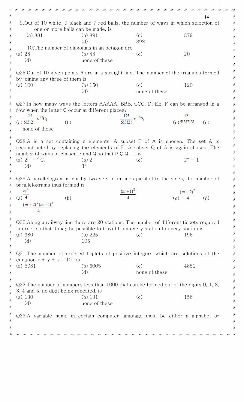
9. Out of 10 white, 9 black and 7 red balls, the number of ways in which selection of
one or more balls can be made, is
(a) 881 (b) 891 (c) 879
(d) 892
10. The number of diagonals in an octagon are
(a) 28 (b) 48 (c) 20
(d) none of these
Q26.Out of 10 given points 6 are in a straight line. The number of the triangles formed
by joining any three of them is
(a) 100 (b) 150 (c) 120
(d) none of these
Q27.In how many ways the letters AAAAA, BBB, CCC, D, EE, F can be arranged in a
row when the letter C occur at different places?
(a) (b) (c) (d)
none of these
Q28.A is a set containing n elements. A subset P of A is chosen. The set A is
reconstructed by replacing the elements of P. A subset Q of A is again chosen. The
number of ways of chosen P and Q so that P Ç Q = f is
(a) 22n – 2nCn (b) 2n (c) 2n – 1
(d) 3n
Q29.A parallelogram is cut by two sets of m lines parallel to the sides, the number of
parallelograms thus formed is
(a) (b) (c) (d)
Q30.Along a railway line there are 20 stations. The number of different tickets required
in order so that it may be possible to travel from every station to every station is
(a) 380 (b) 225 (c) 196
(d) 105
Q31.The number of ordered triplets of positive integers which are solutions of the
equation x + y + z = 100 is
(a) 5081 (b) 6005 (c) 4851
(d) none of these
Q32.The number of numbers less than 1000 that can be formed out of the digits 0, 1, 2,
3, 4 and 5, no digit being repeated, is
(a) 130 (b) 131 (c) 156
(d) none of these
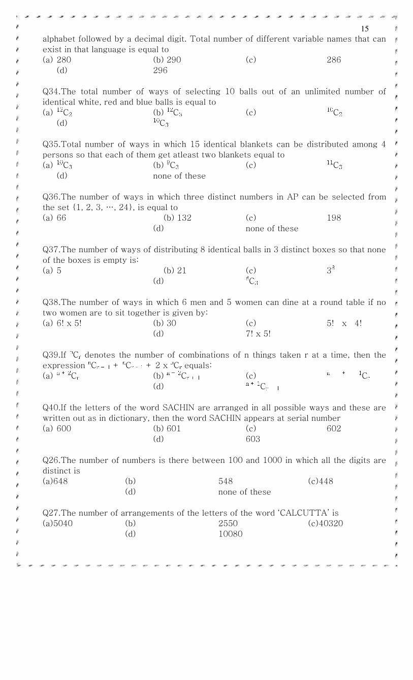
Q33.A variable name in certain computer language must be either a alphabet or
15
alphabet followed by a decimal digit. Total number of different variable names that can
exist in that language is equal to
(a) 280 (b) 290 (c) 286
(d) 296
Q34.The total number of ways of selecting 10 balls out of an unlimited number of
identical white, red and blue balls is equal to
(a) 12C2 (b) 12C3 (c) 10C2 (d) 10C3
Q35.Total number of ways in which 15 identical blankets can be distributed among 4
persons so that each of them get atleast two blankets equal to
(a) 10C3 (b) 9C3 (c) 11C3
(d) none of these
Q36.The number of ways in which three distinct numbers in AP can be selected from
the set {1, 2, 3, …, 24}, is equal to
(a) 66 (b) 132 (c) 198
(d) none of these
Q37.The number of ways of distributing 8 identical balls in 3 distinct boxes so that none
of the boxes is empty is:
(a) 5 (b) 21 (c) 38
(d) 8C3
Q38.The number of ways in which 6 men and 5 women can dine at a round table if no
two women are to sit together is given by:
(a) 6! x 5! (b) 30 (c) 5! x 4!
(d) 7! x 5!
Q39.If nCr denotes the number of combinations of n things taken r at a time, then the
expression nCr + 1 + nCr – 1 + 2 x nCr equals:
(a) n + 2Cr (b) n + 2Cr + 1 (c) n + 1Cr (d) n + 1Cr + 1
Q40.If the letters of the word SACHIN are arranged in all possible ways and these are
written out as in dictionary, then the word SACHIN appears at serial number
(a) 600 (b) 601 (c) 602
(d) 603
Q26.The number of numbers is there between 100 and 1000 in which all the digits are
distinct is
(a) 648 (b) 548 (c) 448
(d) none of these
Q27.The number of arrangements of the letters of the word ‘CALCUTTA’ is
(a) 5040 (b) 2550 (c) 40320
(d) 10080
16
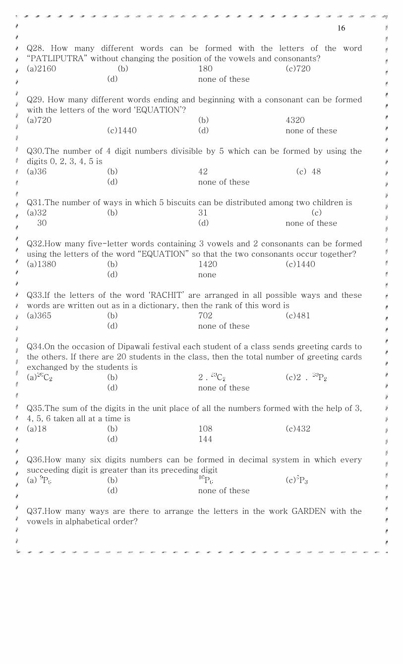
Q28. How many different words can be formed with the letters of the word
“PATLIPUTRA” without changing the position of the vowels and consonants?
(a) 2160 (b) 180 (c) 720
(d) none of these
Q29. How many different words ending and beginning with a consonant can be formed
with the letters of the word ‘EQUATION’?
(a) 720 (b) 4320
(c) 1440 (d) none of these
Q30.The number of 4 digit numbers divisible by 5 which can be formed by using the
digits 0, 2, 3, 4, 5 is
(a) 36 (b) 42 (c) 48
(d) none of these
Q31.The number of ways in which 5 biscuits can be distributed among two children is
(a) 32 (b) 31 (c)
30 (d) none of these
Q32.How many five-letter words containing 3 vowels and 2 consonants can be formed
using the letters of the word “EQUATION” so that the two consonants occur together?
(a) 1380 (b) 1420 (c) 1440
(d) none
Q33.If the letters of the word ‘RACHIT’ are arranged in all possible ways and these
words are written out as in a dictionary, then the rank of this word is
(a) 365 (b) 702 (c) 481
(d) none of these
Q34.On the occasion of Dipawali festival each student of a class sends greeting cards to
the others. If there are 20 students in the class, then the total number of greeting cards
exchanged by the students is
(a) 20C2 (b) 2 . 20C2 (c) 2 . 20P2
(d) none of these
Q35.The sum of the digits in the unit place of all the numbers formed with the help of 3,
4, 5, 6 taken all at a time is
(a) 18 (b) 108 (c) 432
(d) 144
Q36.How many six digits numbers can be formed in decimal system in which every
succeeding digit is greater than its preceding digit
(a) 9P6 (b) 10P6 (c) 9P3
(d) none of these
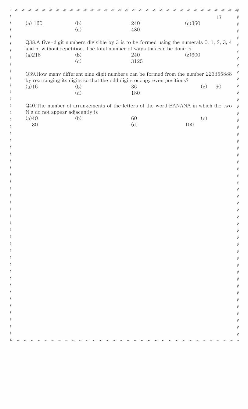
Q37.How many ways are there to arrange the letters in the work GARDEN with the
vowels in alphabetical order?
17
(a) 120 (b) 240 (c) 360
(d) 480
Q38.A five-digit numbers divisible by 3 is to be formed using the numerals 0, 1, 2, 3, 4
and 5, without repetition. The total number of ways this can be done is
(a) 216 (b) 240 (c) 600
(d) 3125
Q39.How many different nine digit numbers can be formed from the number 223355888
by rearranging its digits so that the odd digits occupy even positions?
(a) 16 (b) 36 (c) 60
(d) 180
Q40.The number of arrangements of the letters of the word BANANA in which the two
N’s do not appear adjacently is
(a) 40 (b) 60 (c)
80 (d) 100
18
THE BINOMIAL THEOREMTHE BINOMIAL THEOREMTHE BINOMIAL THEOREMTHE BINOMIAL THEOREM
Binomial expressionBinomial expressionBinomial expressionBinomial expression:
An algebraic expression consisting of only two terms is called a binomial
expression.
ExExExEx: i) x+y ii) 4x -3y iii) x2+y2 iv) x2- 1/a2 Binomial theoremBinomial theoremBinomial theoremBinomial theorem:
The formula by which any power of a binomial expression can be
expanded in the form of a series is known as binomial theorem. This theorem
is given by Sir Issac Newton.
Binomial theorem for positive integral indexBinomial theorem for positive integral indexBinomial theorem for positive integral indexBinomial theorem for positive integral index:
If n is a positive integer
=+ nyx )( +0
0 yxcnn +− 11
1 yxc nn +− 22
2 yxc nn +− 33
3 yxcnn ……………..+ nnn
n
nyxc
−
Note: Note: Note: Note:
1) Number of terms in the expansion of (x + y)n is n+1.
2) In the expansion of (x + y)n, the sum of the powers of x and y is equal to n.
3) 0cn , 1cn , 2cn ,………, n
nc are called coefficients of 1st, 2nd ,……..,(n+1)th terms
respectively. These are called binomial coefficients.
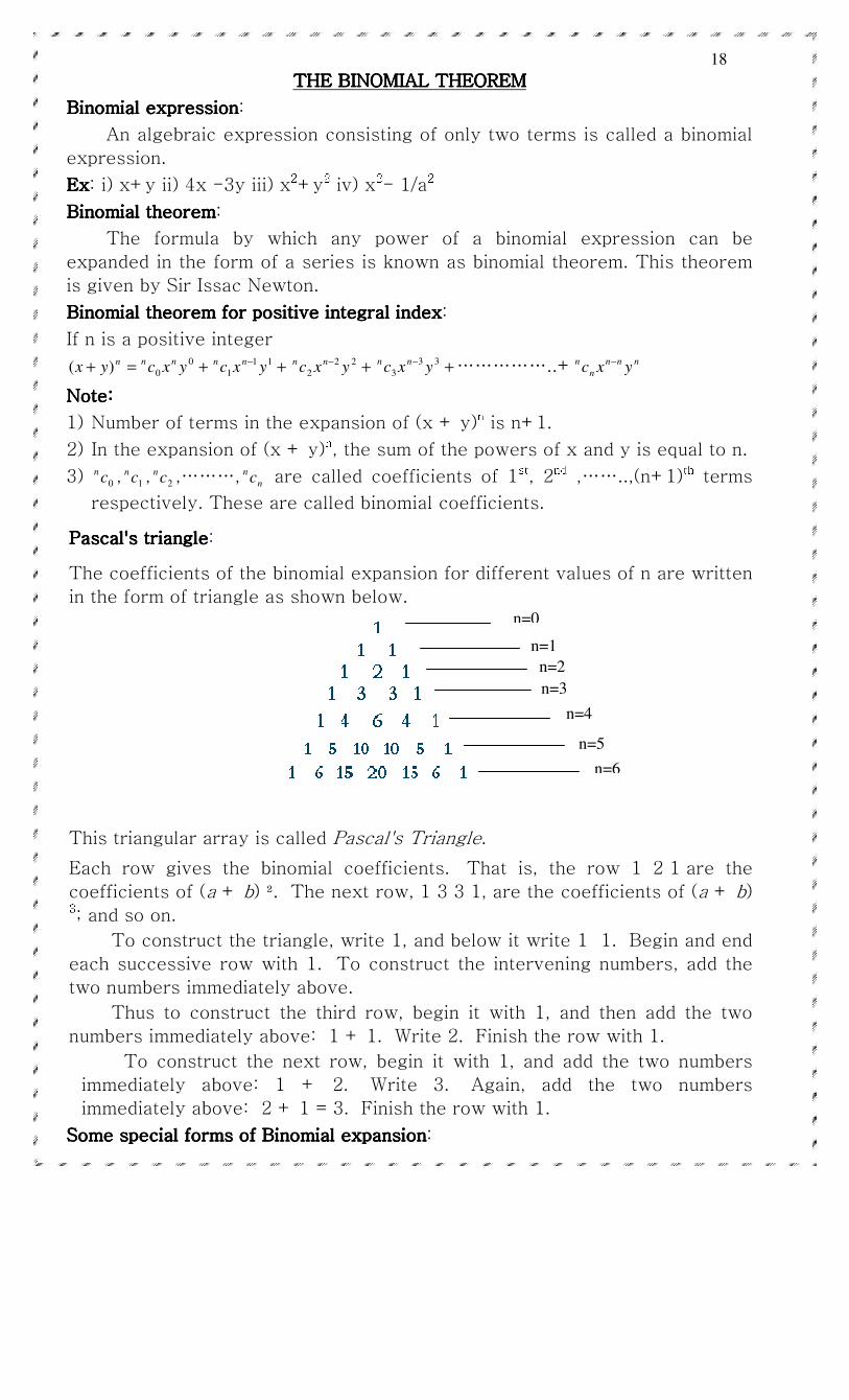
Pascal's trianglePascal's trianglePascal's trianglePascal's triangle:
The coefficients of the binomial expansion for different values of n are written
in the form of triangle as shown below.
This triangular array is called Pascal's Triangle.
Each row gives the binomial coefficients. That is, the row 1 2 1 are the
coefficients of (a + b) ². The next row, 1 3 3 1, are the coefficients of (a + b) 3; and so on.
To construct the triangle, write 1, and below it write 1 1. Begin and end
each successive row with 1. To construct the intervening numbers, add the
two numbers immediately above.
Thus to construct the third row, begin it with 1, and then add the two
numbers immediately above: 1 + 1. Write 2. Finish the row with 1.
To construct the next row, begin it with 1, and add the two numbers
immediately above: 1 + 2. Write 3. Again, add the two numbers
immediately above: 2 + 1 = 3. Finish the row with 1.
Some special forms of Binomial expansionSome special forms of Binomial expansionSome special forms of Binomial expansionSome special forms of Binomial expansion:
n=0
n=1
n=2
n=3
n=4
n=5
n=6
19
=+ nyx )( +0
0 yxcnn +− 11
1 yxc nn +− 22
2 yxc nn +− 33
3 yxcnn …………+ nnn
n
nyxc
− … (1)
=∑=
n
r 0
rrn
r
n yxc −
Put –x in place of x, we get
=− nyx )( −0
0 yxcnn +− 11
1 yxc nn −− 22
2 yxc nn +− 33
3 yxcnn ……+ nnn
n
nnyxc
−− )1( …(2)
= ∑=
−n
r
r
0
)1( rrn
r
n yxc −
Put x = 1 in (1)
=+ ny)1( +0
01 ycnn +− 11
11 yc nn +− 22
21 yc nn +− 33
31 ycnn …………+ nnn
n
nyc
−1
= +1 +ycn
1 +2
2 ycn +3
3 ycn …………+ ny
= ∑=
n
r 0
r
r
n yc
Put x = 1 in (2)
=− ny)1( −0
01 ycnn +− 11
11 yc nn −− 22
21 yc nn +− 33
31 ycnn …………+ nnn
n
nnyc
−− 1)1(
= −1 +ycn
1 −2
2 ycn +3
3 ycn …………+ nn y)1(−
= ∑=
−n
r
r
0
)1( r
r
n yc
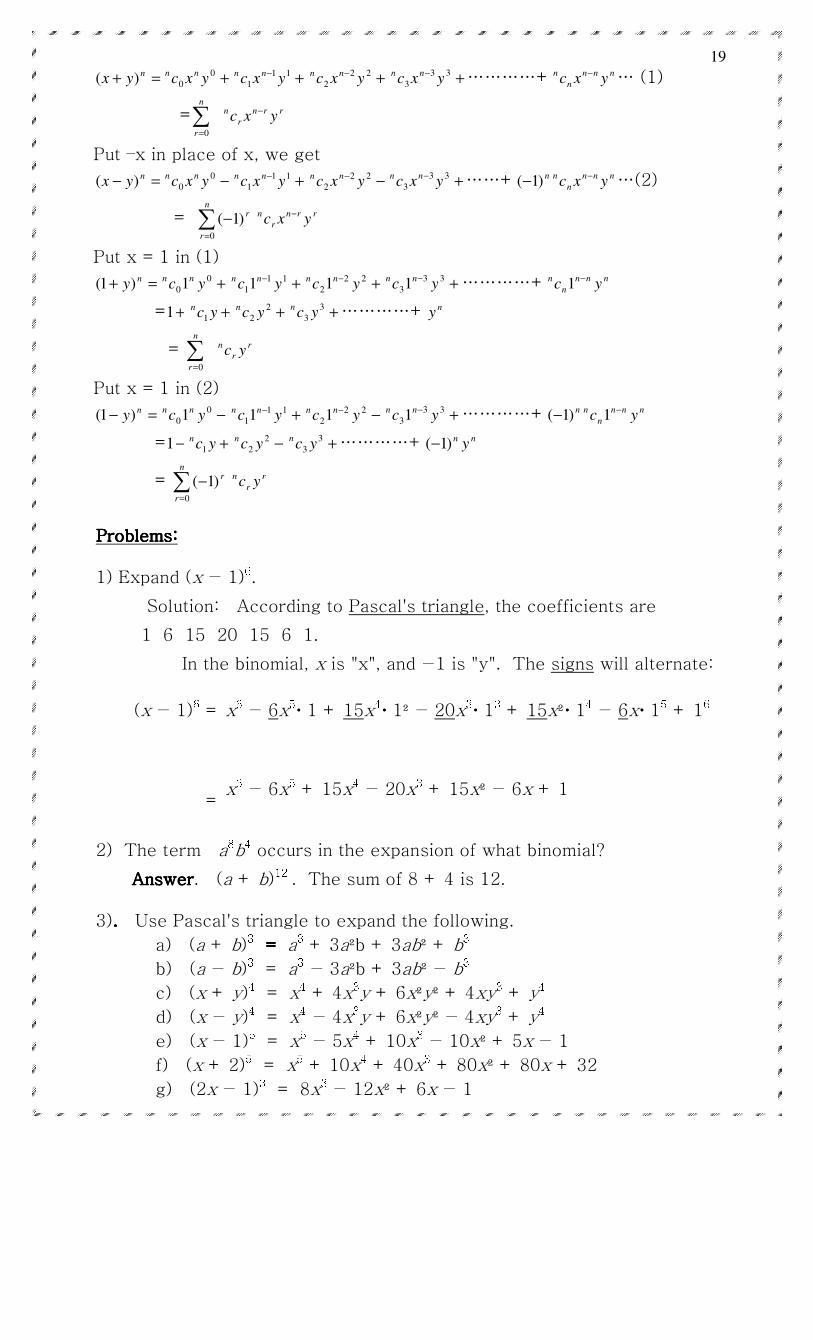
Problems:Problems:Problems:Problems:
1) Expand (x − 1)6. Solution: According to Pascal's triangle, the coefficients are
1 6 15 20 15 6 1.
In the binomial, x is "x", and −1 is "y". The signs will alternate:
(x − 1)6 =
x6 − 6x5
···· 1 + 15x4···· 1² − 20x3
···· 13 + 15x²···· 14 − 6x···· 15 + 16
= x
6 − 6x5 + 15x4 − 20x3 + 15x² − 6x + 1
2) The term a8b
4 occurs in the expansion of what binomial?
AnswerAnswerAnswerAnswer. (a + b)12 . The sum of 8 + 4 is 12.
3).... Use Pascal's triangle to expand the following.
a) (a + b)3 = = = = a3 + 3a²b + 3ab² + b3
b) (a − b)3 = a3 − 3a²b + 3ab² − b3 c) (x + y)4 = x4 + 4x3
y + 6x²y² + 4xy3 + y4 d) (x − y)4 = x4 − 4x3
y + 6x²y² − 4xy3 + y4 e) (x − 1)5 = x5 − 5x4 + 10x3 − 10x² + 5x − 1
f) (x + 2)5 = x5 + 10x4 + 40x3 + 80x² + 80x + 32
g) (2x − 1)3 = 8x3 − 12x² + 6x − 1
20
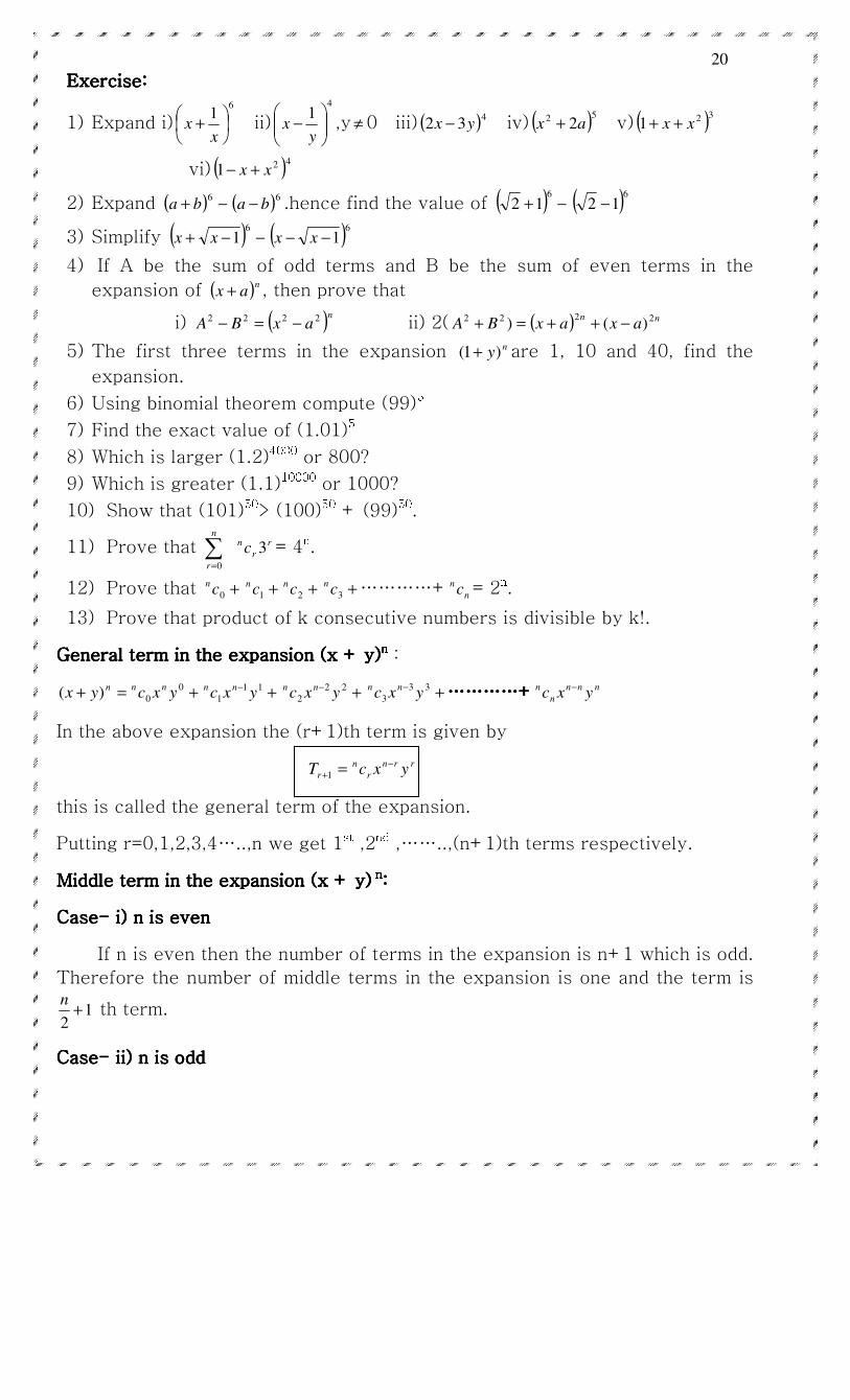
Exercise:Exercise:Exercise:Exercise:
1) Expand i)6
1
+
xx ii)
4
1
−
yx ,y≠ 0 iii) ( )4
32 yx − iv) ( )52 2ax + v) ( )321 xx ++
vi) ( )421 xx +−
2) Expand ( ) −+6
ba ( )6ba − .hence find the value of ( ) −+
6
12 ( )6
12 −
3) Simplify ( ) −−+6
1xx ( )6
1−− xx
4) If A be the sum of odd terms and B be the sum of even terms in the
expansion of ( )nax + , then prove that
i) ( )naxBA 2222 −=− ii) 2( ( ) nn
axaxBA 2222 )() −++=+
5) The first three terms in the expansion ny)1( + are 1, 10 and 40, find the
expansion.
6) Using binomial theorem compute (99)5 7) Find the exact value of (1.01)5 8) Which is larger (1.2)4000 or 800?
9) Which is greater (1.1)10000 or 1000?
10) Show that (101)50> (100)50 + (99)50. 11) Prove that ∑
=
n
r 0
r
r
nc 3 = 4n. 12) Prove that +0c
n +1cn +2cn +3cn …………+ n
nc = 2n.
13) Prove that product of k consecutive numbers is divisible by k!.
General term in the expansion (x + y)General term in the expansion (x + y)General term in the expansion (x + y)General term in the expansion (x + y)nnnn : =+ nyx )( +0
0 yxcnn +− 11
1 yxc nn +− 22
2 yxc nn +− 33
3 yxcnn …………+…………+…………+…………+ nnn
n
nyxc
−
In the above expansion the (r+1)th term is given by
=+1rT rrn
r
n yxc −
this is called the general term of the expansion.
Putting r=0,1,2,3,4…..,n we get 1st ,2nd ,……..,(n+1)th terms respectively.
Middle term in the expansionMiddle term in the expansionMiddle term in the expansionMiddle term in the expansion (x + y)(x + y)(x + y)(x + y) nnnn:::: CaseCaseCaseCase---- i) n is eveni) n is eveni) n is eveni) n is even
If n is even then the number of terms in the expansion is n+1 which is odd.
Therefore the number of middle terms in the expansion is one and the term is
12
+n
th term.
CaseCaseCaseCase---- ii) n is oddii) n is oddii) n is oddii) n is odd

21
If n is odd then the number of terms in the expansion is n+1 which is even.
Therefore the number middle terms in the expansion are two and the terms are
2
1+nth and
2
3+nth terms.
Greatest coefficient in the expansionGreatest coefficient in the expansionGreatest coefficient in the expansionGreatest coefficient in the expansion (x + y)(x + y)(x + y)(x + y)n n n n :::: In any binomial expansion the middle term has the greatest coefficient. If
there are two middle terms then their two coefficients are equal and greater.
ProbProbProbProb : If n be a positive integer, prove that the coefficients of the terms in the
expansion of (x+y)n equidistant from the beginning and from the end are equal.
In the expansion of (x+y)n Co efficient of 1st term from beginning = 0c
n
Co efficient of 2nd term from beginning = 1cn
Co efficient of 3rd term from beginning = 2cn
……………………………………..
………………………………………
Co efficient of r th term from beginning = 1−r
nc
Now
Co efficient of 1st term from end = n
nc
Co efficient of 2nd term from end = 1−n
nc
Co efficient of 3rd term from end = 2−n
nc
……………………………………..
………………………………………
Co efficient of r th term from end = )1( −− rn
nc
Since 1−r
nc = = = = )1( −− rn
nc are equal. We can say in the expansion of (x+y)n , the co
efficient of r th term from beginning and end are equal.
NoteNoteNoteNote: In the binomial expansion, the r th term from the end is equal to (nIn the binomial expansion, the r th term from the end is equal to (nIn the binomial expansion, the r th term from the end is equal to (nIn the binomial expansion, the r th term from the end is equal to (n----r+2)th r+2)th r+2)th r+2)th
term from the beginning.term from the beginning.term from the beginning.term from the beginning.
ProblemsProblemsProblemsProblems:
1) Find the 4 th term in the expansion of (x-2y)12 2) Find the 13 th term in the expansion of .0,
3
19
18
≠
− x
xx
22
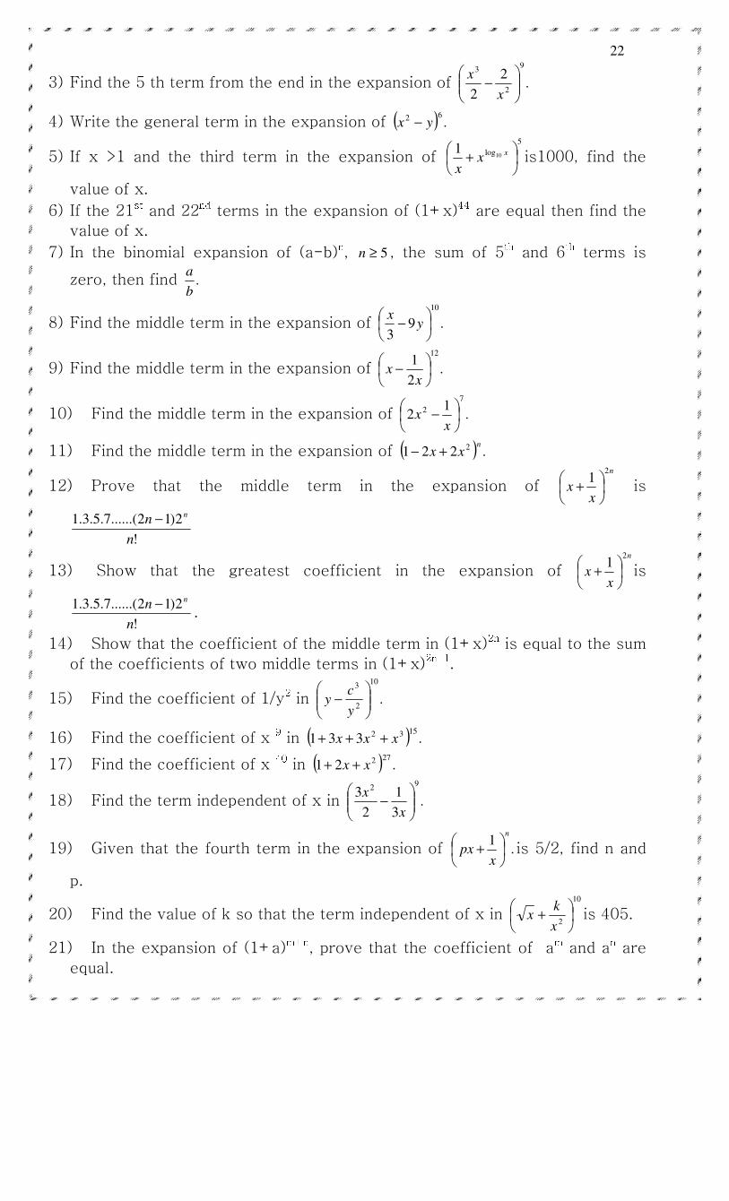
3) Find the 5 th term from the end in the expansion of .2
2
9
2
3
−
x
x
4) Write the general term in the expansion of ( ) .62 yx −
5) If x >1 and the third term in the expansion of 5
log101
+ x
xx
is1000, find the
value of x.
6) If the 21st and 22nd terms in the expansion of (1+x)44 are equal then find the
value of x.
7) In the binomial expansion of (a-b)n, 5≥n , the sum of 5th and 6th terms is
zero, then find .b
a
8) Find the middle term in the expansion of .93
10
− y
x
9) Find the middle term in the expansion of .2
112
−
xx
10) Find the middle term in the expansion of .1
2
7
2
−
xx
11) Find the middle term in the expansion of ( ) .221 2 nxx +−
12) Prove that the middle term in the expansion of n
xx
21
+ is
!
2)12......(7.5.3.1
n
nn−
13) Show that the greatest coefficient in the expansion of n
xx
21
+ is
!
2)12......(7.5.3.1
n
nn−
.
14) Show that the coefficient of the middle term in (1+x)2n is equal to the sum
of the coefficients of two middle terms in (1+x)2n-1. 15) Find the coefficient of 1/y2 in .
10
2
3
−
y
cy
16) Find the coefficient of x 9 in ( ) .3311532 xxx +++
17) Find the coefficient of x 40 in ( ) .21272xx ++
18) Find the term independent of x in .3
1
2
39
2
−
x
x
19) Given that the fourth term in the expansion of .1
n
xpx
+ is 5/2, find n and
p.
20) Find the value of k so that the term independent of x in 10
2
+
x
kx is 405.
21) In the expansion of (1+a)m+n, prove that the coefficient of am and an are
equal.
23
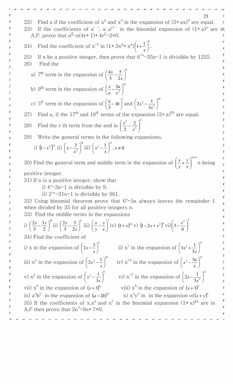
22) Find a if the coefficient of x2 and x3 in the expansion of (3+ax)9 are equal.
23) If the coefficients of ar-1, ar,ar+1 in the binomial expansion of (1+a)n are in
A.P. prove that n2-n(4r+1)+4r2-2=0.
24) Find the coefficient of x-1 in (1+3x2+x4) 81
1
+
x.
25) If n be a positive integer, then prove that 62n-35n-1 is divisible by 1225.
26) Find the
a) 7th term in the expansion of 9
2
5
5
4
−
x
x
b) 9th term in the expansion of 12
2
3
−
x
a
a
x
c) 5th term in the expansion of 7
33
− b
aand
10
3
2
3
12
−
xx
27) Find a, if the 17th and 18th terms of the expansion (2+a)50 are equal.
28) Find the r th term from the end in
9
2
3 2
2
−
x
x
29) Write the general terms in the following expansions.
i) ( ) .1122x− ii)
10
2
3
−
xx iii)
12
2 1
−
xx , 0≠x
30) Find the general term and middle term in the expansion of
12 +
+
n
x
y
y
xn being
positive integer.
31) If n is a positive integer, show that
i) 4n-3n-1 is divisible by 9.
ii) 25n-31n-1 is divisible by 961.
32) Using binomial theorem prove that 6n-5n always leaves the remainder 1
when divided by 25 for all positive integers n.
33) Find the middle terms in the expansions
i) 20
2
3
3
2
−
yxii)
6
2
3
3
2
−
x
x iii)
7
−
x
y
y
xiv) ( ) n
x2
1+ v) ( )nxx 221 +− vi)
73
63
−
x
34) Find the coefficient of
i) x in the expansion of 9
32
−
xx ii) x7 in the expansion of
11
2
5
13
+
xx
iii) x9 in the expansion of 20
2 12
−
xx iv) x24 in the expansion of
15
2 3
−
x
ax
v) x9 in the expansion of 9
2
3
1
−
xx vi) x-7 in the expansion of
11
23
12
−
xx
vii) x5 in the expansion of ( )83+x viii) x5 in the expansion of ( )9
3+x
ix) a5b7 in the expansion of ( )122ba − x) x6y3 in in the expansion of ( )9
yx +
35) If the coefficients of x,x2 and x3 in the binomial expansion (1+x)2n are in
A.P then prove that 2n2-9n+7=0.
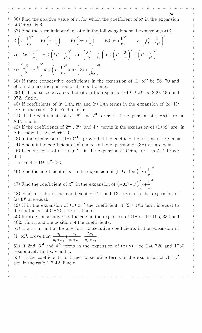
24
36) Find the positive value of m for which the coefficient of x2 in the expansion
of (1+x)m is 6.
37) Find the term independent of x in the following binomial expansion(x ≠ 0).
i) n
xx
21
+ ii)
141
−
xx iii)
13
2 12
+
xx iv)
12
2 1
+
xx v)
10
22
3
3
+
x
x
vi) 12
2 12
−
xx vii)
25
3
2 32
−
xx viii)
62
3
1
2
3
−
x
x ix)
15
2
3 3
−
xx x)
10
3
2 3
−
xx
xi)
8
313
1
2
+
−x
xxii)
121
−
xx xiii)
18
3
3
2
1
+
xx
38) If three consecutive coefficients in the expansion of (1+x)n be 56, 70 and
56., find n and the position of the coefficients.
39) If three successive coefficients in the expansion of (1+x)n be 220, 495 and
972., find n.
40) If coefficients of (r-1)th, rth and (r+1)th terms in the expansion of (x+1)n are in the ratio 1:3:5. Find n and r.
41) If the coefficients of 5th, 6th and 7th terms in the expansion of (1+x)n are in
A.P, Find n.
42) If the coefficients of 2nd , 3rd and 4th terms in the expansion of (1+x)n are in
A.P, show that 2n2-9n+7=0.
43) In the expansion of (1+a)m+n, prove that the coefficient of am and an are equal.
44) Find a if the coefficient of x2 and x3 in the expansion of (3+ax)9 are equal.
45) If coefficients of ar-1, ar,ar+1 in the expansion of (1+a)n are in A.P. Prove
that
n2-n(4r+1)+4r2-2=0.
46) Find the coefficient of x4 in the expansion of ( ).1031 2xx ++
101
+
xx
47) Find the coefficient of x-1 in the expansion of ( ).31 42 xx ++
81
+
xx
48) Find n if the if the coefficient of 4th and 13th terms in the expansion of
(a+b)n are equal.
49) If in the expansion of (1+x)43 the coefficient of (2r+1)th term is equal to
the coefficient of (r+2) th term , find r.
50) If three consecutive coefficients in the expansion of (1+x)n be 165, 330 and
462., find n and the position of the coefficients.
51) If a1,a2,a3 and a4 be any four consecutive coefficients in the expansion of
(1+x)n, prove that 32
2
43
3
21
1 2
aa
a
aa
a
aa
a
+=
++
+.
52) If 2nd, 3rd and 4th terms in the expansion of (x+y) n be 240,720 and 1080
respectively find x, y and n.
53) If the coefficients of three consecutive terms in the expansion of (1+a)n are in the ratio 1:7:42. Find n .
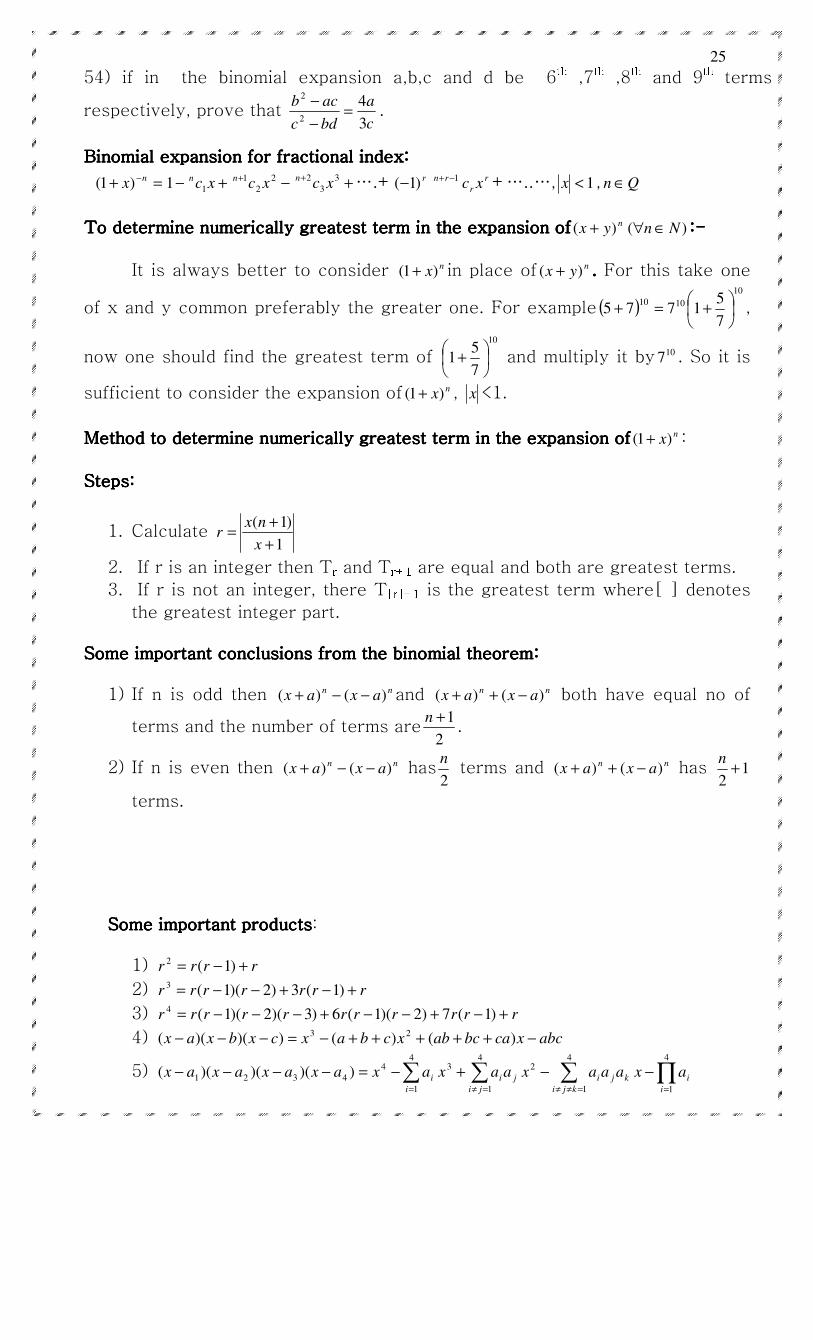
25
54) if in the binomial expansion a,b,c and d be 6th ,7th ,8th and 9th terms
respectively, prove that c
a
bdc
acb
3
42
2
=−
−.
Binomial expansion for fractional index:Binomial expansion for fractional index:Binomial expansion for fractional index:Binomial expansion for fractional index:
=+ −nx)1( −1 +xcn
1 −+ 2
2
1 xcn ++ 3
3
2xc
n ….+ r
r
rnr xc1)1( −+− +…..…, 1<x , Qn ∈
To determine numerically greatest term in the expansion ofTo determine numerically greatest term in the expansion ofTo determine numerically greatest term in the expansion ofTo determine numerically greatest term in the expansion of nyx )( + )( Nn ∈∀ ::::----
It is always better to consider nx)1( + in place of nyx )( + . . . . For this take one
of x and y common preferably the greater one. For example ( )10
1010
7
51775
+=+ ,
now one should find the greatest term of 10
7
51
+ and multiply it by 107 . So it is
sufficient to consider the expansion of nx)1( + , x <1.
Method to determine numerically greatest term in the expansion ofMethod to determine numerically greatest term in the expansion ofMethod to determine numerically greatest term in the expansion ofMethod to determine numerically greatest term in the expansion of nx)1( + :
Steps:Steps:Steps:Steps:
1. Calculate 1
)1(
+
+=
x
nxr
2. If r is an integer then Tr and Tr+1 are equal and both are greatest terms.
3. If r is not an integer, there T[r]+1 is the greatest term where[ ] denotes
the greatest integer part.
Some important conclusions frSome important conclusions frSome important conclusions frSome important conclusions from the binomial theorem:om the binomial theorem:om the binomial theorem:om the binomial theorem:
1) If n is odd then nn axax )()( −−+ and nn axax )()( −++ both have equal no of
terms and the number of terms are2
1+n.
2) If n is even then nn axax )()( −−+ has2
n terms and nn axax )()( −++ has 1
2+
n
terms.
Some important productsSome important productsSome important productsSome important products:
1) rrrr +−= )1(2
2) rrrrrrr +−+−−= )1(3)2)(1(3
3) rrrrrrrrrrr +−+−−+−−−= )1(7)2)(1(6)3)(2)(1(4
4) abcxcabcabxcbaxcxbxax −+++++−=−−− )()())()(( 23
5) ∑ ∑ ∑ ∏= =≠ =≠≠ =
−−+−=−−−−4
1
4
1
4
1
4
1
234
4321 ))()()((i ji kji i
ikjijii axaaaxaaxaxaxaxaxax
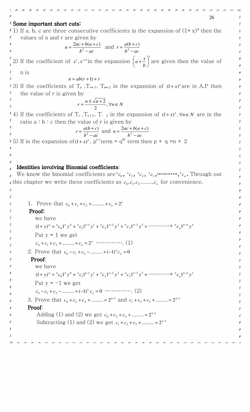
26
Some important short cuts:Some important short cuts:Some important short cuts:Some important short cuts:
1) If a, b, c are three consecutive coefficients in the expansion of (1+x)n then the
values of n and r are given by
acb
cabacn
−
++=
2
)(2 and
acb
cbar
−
+=
2
)(
2) If the coefficient of 1, +rr xx in the expansion n
b
xa
+ are given then the value of
n is rrabn ++= )1(
3) If the coefficients of Tr ,Tr+1, Tr+2 in the expansion of nx)1( + are in A.P then
the value of r is given by
Nnnn
r ∈∀+±
= ,2
2
4) If the coefficients of Tr ,Tr+1, Tr+2 in the expansion of nx)1( + , Nn ∈∀ are in the
ratio a : b : c then the value of r is given by
acb
cbar
−
+=
2
)( and
acb
cabacn
−
++=
2
)(2
5) If in the expansion of nx)1( + , pth term = qth term then p + q =n + 2
Identities involving Binomial coefficientsIdentities involving Binomial coefficientsIdentities involving Binomial coefficientsIdentities involving Binomial coefficients:
We know the binomial coefficients are 0cn , , , , 1cn , , , , 2cn ,,,, 3c
n ,…………,,…………,,…………,,…………, n
nc . . . . Through out
this chapter we write these coefficients as ncccc ,..........,, 210 for convenience.
1. Prove that n
ncccc 2..........210 =++++
Proof: Proof: Proof: Proof:
we have
=+ ny)1( +0
01 ycnn +− 11
11 yc nn +− 22
21 yc nn +− 33
31 ycnn …………+ nnn
n
nyc
−1
Put y = 1 we get n
ncccc 2..........210 =++++ ……………. (1)
2. Prove that 0)1(..........210 =−+−+− n
ncccc
ProofProofProofProof:
we have
=+ ny)1( +0
01 ycnn +− 11
11 yc nn +− 22
21 yc nn +− 33
31 ycnn …………+ nnn
n
nyc
−1
Put y = -1 we get
0)1(..........210 =−+−+− n
ncccc ……………. (2)
3. Prove that 1
420 2.......... −=+++ nccc and 1
531 2.......... −=+++ nccc
ProofProofProofProof:
Adding (1) and (2) we get 1
420 2.......... −=+++ nccc
Subtracting (1) and (2) we get 1
531 2.......... −=+++ nccc
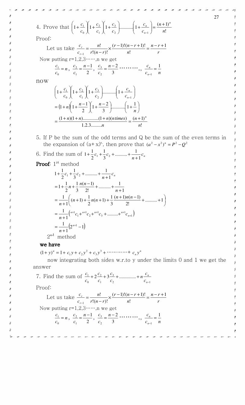
27
4. Prove that !
)1(1............111
12
3
1
2
0
1
n
n
c
c
c
c
c
c
c
c n
n
n +=
+
+
+
+
−
Proof:
Let us take r
rn
n
rnr
rnr
n
c
c
r
r 1
!
)!1()!1(
)!(!
!
1
+−=
+−−×
−=
−
Now putting r=1,2,3……,n we get
nc
c=
0
1 , 2
1
1
2 −=
n
c
c,
3
2
2
3 −=
n
c
c……….,
nc
c
n
n 1
1
=−
now
( )
!
)1(
.........3.2.1
))(1....().........1)(1(
11............
3
21
2
111
1............11112
3
1
2
0
1
n
n
n
timesnnnn
n
nnn
c
c
c
c
c
c
c
c
n
n
n
+=
+++=
+
−+
−++=
+
+
+
+
−
5. If P be the sum of the odd terms and Q be the sum of the even terms in
the expansion of (a+x)n, then prove that 2222 )( QPxa n −=−
6. Find the sum of ncn
cc1
1..........
3
1
2
11 21
+++++
ProofProofProofProof: 1st method
( )
( )121
1
.........1
1
1..........!2
)1()1(
3
1)1(
2
1)1(
1
1
1
1..........
!2
)1(
3
1
2
11
1
1..........
3
1
2
11
1
1
1
3
1
2
1
1
1
21
−+
=
+++++
=
++
−+++++
+=
+++
−++=
+++++
+
+
++++
n
n
nnnn
n
n
ccccn
nnnnnn
n
n
nnn
cn
cc
2nd method
we have we have we have we have
=+ ny)1( +1 +yc1 +2
2 yc +3
3 yc …………+ n
n yc
now integrating both sides w.r.to y under the limits 0 and 1 we get the
answer
7. Find the sum of 12
3
1
2
0
1 ..............32−
++++n
n
c
cn
c
c
c
c
c
c
Proof:
Let us take r
rn
n
rnr
rnr
n
c
c
r
r 1
!
)!1()!1(
)!(!
!
1
+−=
+−−×
−=
−
Now putting r=1,2,3……,n we get
nc
c=
0
1 , 2
1
1
2 −=
n
c
c,
3
2
2
3 −=
n
c
c……….,
nc
c
n
n 1
1
=−
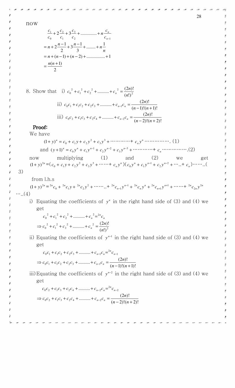
28
now
2
)1(
1................)2()1(
1........
3
13
2
12
..............3212
3
1
2
0
1
+=
++−+−+=
++−
+−
+=
++++−
nn
nnn
nn
nnn
c
cn
c
c
c
c
c
c
n
n
8. Show that i) 2
22
2
2
1
2
0)!(
)!2(..........
n
ncccc n =++++
ii) )!1()!1(
)!2(.......... 1322110
+−=++++ −
nn
ncccccccc nn
iii) )!2()!2(
)!2(.......... 2423120
+−=++++ −
nn
ncccccccc nn
Proof:Proof:Proof:Proof:
We have
=+ ny)1( +0c +yc1 +2
2 yc +3
3 yc …………+ n
n yc ……………. (1)
and =+ ny )1( +nyc0 +−1
1
nyc +−2
2
nyc +−3
3
nyc …………+ nc …………….(2)
now multiplying (1) and (2) we get
ny 2)1( + =( +0c +yc1 +2
2 yc +3
3 yc ……+ n
n yc )( +nyc0 +−1
1
nyc +−2
2
nyc …..+ nc )……..(
3)
from l.h.s ny 2)1( + = +0
2c
n +ycn
1
2 +2
2
2 ycn ……..+ +−
−
1
1
2 n
n
nyc +n
n
nyc
2 ++
+
1
1
2 n
n
nyc ……+ n
n
nyc
2
2
2
…..(4)
i) Equating the coefficients of ny in the right hand side of (3) and (4) we
get
2
22
2
2
1
2
0
222
2
2
1
2
0
)!(
)!2(..........
..........
n
ncccc
ccccc
n
n
n
n
=++++⇒
=++++
ii) Equating the coefficients of 1−ny in the right hand side of (3) and (4) we
get
)!1()!1(
)!2(..........
..........
1322110
1
2
1322110
+−=++++⇒
=++++
−
−−
nn
ncccccccc
ccccccccc
nn
n
n
nn
iii) Equating the coefficients of 2−ny in the right hand side of (3) and (4) we
get
)!2()!2(
)!2(..........
..........
2423120
2
2
2423120
+−=++++⇒
=++++
−
−−
nn
ncccccccc
ccccccccc
nn
n
n
nn
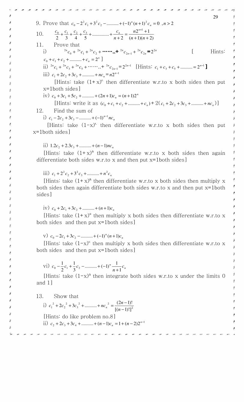
29
9. Prove that 2,0)1()1(..........32 2
2
2
1
2
0 >=+−+−+− ncnccc n
n
10. )2)(1(
12
2..............
5432
1
3210
++
+=
++++++
+
nn
n
n
ccccc n
n
11. Prove that
i) +0
2c
n +1
2 cn +2
2 cn ……..+……..+……..+……..+ +−12
2
n
nc n
nc2
2 ==== n22 [ Hints: n
ncccc 2..........210 =++++ ]
ii) +1
2 cn +3
2c
n +5
2c
n ……..+ 12
2
−n
nc = 122 −n [Hints: 1
531 2.......... −=+++ nccc ]]]]
iii) nncccc ++++ ..........32 321 = 12 −nn
[Hints: take (1+x)n then differentiate w.r.to x both sides then put
x=1both sides]
iv) n
n ncnccc 2)1()12(..........53 210 +=+++++
[Hints: write it as )..........( 210 ncccc ++++ +2( nncccc ++++ ..........32 321 )]
12. Find the sum of
i) n
nncccc
1
321 )1(..........32 −−+−+−
[Hints: take (1-x)n then differentiate w.r.to x both sides then put
x=1both sides]
ii) nncncc )1(..........3.22.1 32 −+++
[Hints: take (1+x)n then differentiate w.r.to x both sides then again
differentiate both sides w.r.to x and then put x=1both sides]
iii) ncnccc2
3
2
2
2
1 ..........32 ++++
[Hints: take (1+x)n then differentiate w.r.to x both sides then multiply x
both sides then again differentiate both sides w.r.to x and then put x=1both
sides]
iv) ncnccc )1(..........32 210 +++++
[Hints: take (1+x)n then multiply x both sides then differentiate w.r.to x
both sides and then put x=1both sides]
v) n
ncnccc )1()1(..........32 210 +−+−+−
[Hints: take (1-x)n then multiply x both sides then differentiate w.r.to x
both sides and then put x=1both sides]
vi) n
nc
nccc
1
1)1(..........
3
1
2
1210
+−+−+−
[Hints: take (1-x)n then integrate both sides w.r.to x under the limits 0
and 1]
13. Show that
i) 2
22
3
2
2
2
1])!1[(
)!12(..........32
−
−=++++
n
nncccc n
[Hints: do like problem no.8]
ii) 1
432 2)2(1)1(..........32 −−+=−++++ n
n ncnccc
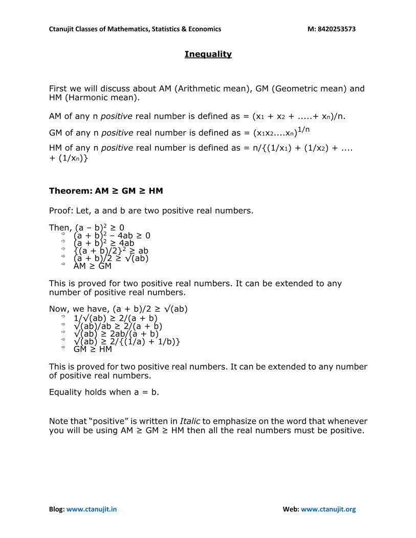
Ctanujit Classes of Mathematics, Statistics & Economics M: 8420253573
Blog: www.ctanujit.in Web: www.ctanujit.org
Inequality
First we will discuss about AM (Arithmetic mean), GM (Geometric mean) and HM (Harmonic mean).
AM of any n positive real number is defined as = (x1 + x2 + .....+ xn)/n.
GM of any n positive real number is defined as = (x1x2....xn)1/n
HM of any n positive real number is defined as = n/{(1/x1) + (1/x2) + .... + (1/xn)}
Theorem: AM ≥ GM ≥ HM
Proof: Let, a and b are two positive real numbers.
Then, (a – b)2 ≥ 0 (a + b)2 – 4ab ≥ 0
(a + b)2 ≥ 4ab
{(a + b)/2}2 ≥ ab
(a + b)/2 ≥ √(ab)
AM ≥ GM
This is proved for two positive real numbers. It can be extended to any number of positive real numbers.
Now, we have, (a + b)/2 ≥ √(ab) 1/√(ab) ≥ 2/(a + b)
√(ab)/ab ≥ 2/(a + b)
√(ab) ≥ 2ab/(a + b)
√(ab) ≥ 2/{(1/a) + 1/b)}
GM ≥ HM
This is proved for two positive real numbers. It can be extended to any number of positive real numbers.
Equality holds when a = b.
Note that “positive” is written in Italic to emphasize on the word that whenever you will be using AM ≥ GM ≥ HM then all the real numbers must be positive.
Ctanujit Classes of Mathematics, Statistics & Economics M: 8420253573
Blog: www.ctanujit.in Web: www.ctanujit.org
Problem 1: Prove that a3 + b3 + c3 ≥ 3abc where a, b, c are positive
real numbers.
Solution 1: Applying AM ≥ GM on a3, b3 and c3 we get,
(a3 + b3 + c3)/3 ≥ (a3b3c3)1/3
(a3 + b3 + c3)/3 ≥ abc
a3 + b3 + c3 ≥ 3abc.
Weighted AM, GM, HM: If x1, x2, ....., xn are n real numbers with weights
w1, w2, ...., wn then weighted AM is defined as,
Weighted AM = (x1w1 + x2w2 + .... + xnwn)/(w1 + w2 + ..... + wn)
Weighted GM = {(x1w1)(x2
w2).....(xnwn)}^{1/(w1 + w2 + .... + wn)}
Weighted HM = (w1 + w2 + .... + wn)/{(w1/x1) + (w2/x2) + .... + (wn/xn)} Also, Weighted AM ≥ Weighted GM ≥ Weighted HM but remember the word positive whenever applying this.
Ctanujit Classes of Mathematics, Statistics & Economics M: 8420253573
Blog: www.ctanujit.in Web: www.ctanujit.org
Combinatorics
Fundamental theorem: If a work can be done in m ways and another work
can be done in n ways then the two works can be done simultaneously in mn ways.
Note: Emphasize on the word simultaneously because most of the students get confused where to apply multiplication and where to apply addition. When both the works need to be done to complete a set of work then apply multiplication and if the works are disjoint then apply addition.
Permutation: There are n things and we need to take r things at a time and
we need to arrange it with respect to order then the total number of ways is nPr where nPr = n!/(n – r)!. For example there are 3 tuples (1, 2, 3) 6 permutations are possible = (1, 2, 3); (1, 3, 2); (2, 1, 3); (2, 3, 1); (3, 1, 2) and (3, 2, 1)
Now, we will check by the formula.
Here number of permutations = 3P3 = 3!/(3 – 3)! = 3×2/1 = 6.
Proof: We can take 1st thing in n ways, 2nd thing in (n – 1) ways, ....., rth
thing in {n – (r – 1)} = (n – r + 1) ways. By fundamental theorem, total number of ways = n(n – 1)(n – 2)....(n – r + 1) = n(n – 1)(n – 2)....(n – r + 1)(n – r)(n – r – 1)....2×1/{(n – r)(n – r – 1)..... ×2×1} (Multiplying numerator and denominator by (n – r)(n – r – 1).... ×2×1) = n!/(n – r)!
So, nPr = n!/(n – r)! Proved.
Ctanujit Classes of Mathematics, Statistics & Economics M: 8420253573
Blog: www.ctanujit.in Web: www.ctanujit.org
Combination: If there are n things and we need to select r things at a time
(order is not important) then total number of ways of doing this = nCr =
n!/(n – r)! ×r!. For example, there are 5 numbers (1, 2, 3, 4, 5). We need to select 3 at a time. Total number of ways = (1, 2, 3); (1, 2, 4); (1, 2, 5); (1, 3, 4); (1, 3, 5); (1, 4, 5); (2, 3, 4); (2, 3, 5); (2, 4, 5); (3, 4, 5) i.e. 10 number of ways.
Now, we will check by formula.
Here number of combinations = 5C3 = 5!/(5 – 3)! ×2! = 5×4×3!/3! ×2 = 10.
Note that here (1, 2, 3) is equivalent to (1, 3, 2) etc. as order is not important in combination but this is important in permutation.
Proof: Now, the order is not important. Hence the number of ways r things can permutate among themselves is r!.
Therefore, r! ×nCr = nPr = n!/(n – r)!
nCr = n!/{(n – r)! × r!} Proved.
Number of non-negative solution:
Problem: a1 + a2 +....+ ar = n where a1, a2, ...., an, n are all integers.
Prove that the number of non-negative solution of the equation is n+r-1Cr-1 (or, (𝒏+𝒓−𝟏
𝒓−𝟏) )
We will prove it by induction.
Clearly, this is true for r = 1. Let, this is true for r = k i.e. number of non-negative solution when there
are k variables in the LHS is (n + k – 1)C(k – 1). Now, number of non-negative solution for r = k + 1 i.e. when an extra variable
gets added in LHS is ∑ (𝑛−𝑖+𝑘−1𝑘−1
)𝑛𝑖=0
Now, we have to prove that, ∑ (𝑛−𝑖+𝑘−1𝑘−1
)𝑛𝑖=0 = (𝑛+𝑘
𝑘).
Now, we will prove this by another induction. For, n = 1,
LHS = kC(k – 1) + (k – 1)C(k – 1) = k + 1
RHS = (k + 1)Ck = k + 1.

Ctanujit Classes of Mathematics, Statistics & Economics M: 8420253573
Blog: www.ctanujit.in Web: www.ctanujit.org
So, this is true for n = 1. Let, this is true for n = p i.e. we have, ∑ (𝑝−𝑖+𝑘−1
𝑘−1)
𝑝𝑖=0 = (𝑝+𝑘
𝑘).
For, n = p + 1, LHS = ∑ (𝑝+1−𝑖+𝑘−1
𝑘−1)
𝑝+1𝑖=0
= (p + k)C(k – 1) + ∑ (𝑝−𝑖+𝑘−1𝑘−1
)𝑝𝑖=0
= (p + k)C(k – 1) + (p + k)Ck = (p + k)!/{(p + 1)!×(k – 1)!} + (p + k)!/{p!×k!} = [(p + k)!/{(p + 1)!×k!}](k + p + 1) = (p + k + 1)!/{(p + 1)!×k!}
= (𝑝+1+𝑘𝑘)
= RHS for n = p + 1.
Number of positive solutions:
Problem: a1 + a2 + … + ar = n where a1, a2, …, ar, n are all positive integers. Prove that number of positive solutions of this equation is n-1Cr-1.
Solution: We will prove this by induction.
Clearly this is true for r = 1.
Let this is true for r = k i.e. if there are k number of variables in LHS then
number of solutions of the equation is n-1Ck-1. Now, for r = k + 1 i.e. if an extra variable gets added then number of solutions of the equation is ∑ (𝑛−𝑖−1
𝑘−1)𝑛−𝑘
𝑖=1
We have to prove that, ∑ (𝑛−𝑖−1𝑘−1
)𝑛−𝑘 𝑖=1 = n-1Ck. We will prove this by
another induction.
Clearly this is true for n = 1.
Let this is true for n = p i.e. ∑ (𝑝−𝑖−1𝑘−1
)𝑝−𝑘 𝑖=1 = p-1Ck.
Now, for n = p + 1, LHS = ∑ (𝑝−𝑖𝑘−1)𝑛−𝑘+1
𝑖=1 = p-1Ck-1 + p-1Ck (from above)
= pCk = RHS for n = p + 1.
Proved.
Ctanujit Classes of Mathematics, Statistics & Economics M: 8420253573
Blog: www.ctanujit.in Web: www.ctanujit.org
Problem: Find number of terms in the expansion of (x + y + z + w)n.
Solution: Now, there are 4 variables and any term consists of the 4 terms such that, x1 + y1 + z1 + w1 = n where x1, y1, z1, w1 are powers of x, y, z, w in any term.
Now, x1, y1, z1, w1 runs from 0 to n. So, we need to find number of non-negative solution of this equation and we are done with number of terms of this equation.
From previous article we know, number of non-negative solution of this
equation = n+4-1C4-1 = n+3C3.
In general if there are r variables then number of terms = n+r-1Cr-1.
Problem: Find number of terms which are independent of x in the
expansion of (x + y + z + w)n.
Solution: Now, x1 = 0. So, we need to find number of non-negative solution of the
equation, y1 + z 1 + w1 = n and then we need to subtract this from n+3C3 and we are done with the number of terms which are independent of x.
It is, n+3-1C3-1 = n+2C2.
So, number of terms which are independent of x = n+3C3 – n+2C2. In general if there are r variables then number of terms excluding one
variable = n+r-1Cr-1 – n+r-2Cr-2. Similarly, we can find number of terms independent of x and y and so on.
Problem: Prove that number of ways of distributing n identical things
among r members where every member gets at least 1 thing is n-1Cr-1.
Solution: Let, first member gets x1 things, second member gets x2 things
and so on i.e. tth member gets xt things. So, x1 + x2 + … + xr = n
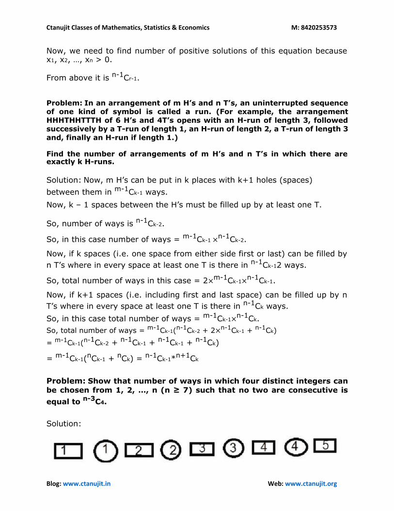
Ctanujit Classes of Mathematics, Statistics & Economics M: 8420253573
Blog: www.ctanujit.in Web: www.ctanujit.org
Now, we need to find number of positive solutions of this equation because x1, x2, …, xn > 0.
From above it is n-1Cr-1.
Problem: In an arrangement of m H’s and n T’s, an uninterrupted sequence of one kind of symbol is called a run. (For example, the arrangement
HHHTHHTTTH of 6 H’s and 4T’s opens with an H-run of length 3, followed successively by a T-run of length 1, an H-run of length 2, a T-run of length 3
and, finally an H-run if length 1.)
Find the number of arrangements of m H’s and n T’s in which there are exactly k H-runs.
Solution: Now, m H’s can be put in k places with k+1 holes (spaces)
between them in m-1Ck-1 ways. Now, k – 1 spaces between the H’s must be filled up by at least one T.
So, number of ways is n-1Ck-2.
So, in this case number of ways = m-1Ck-1 ×n-1Ck-2. Now, if k spaces (i.e. one space from either side first or last) can be filled by
n T’s where in every space at least one T is there in n-1Ck-12 ways.
So, total number of ways in this case = 2×m-1Ck-1×n-1Ck-1. Now, if k+1 spaces (i.e. including first and last space) can be filled up by n
T’s where in every space at least one T is there in n-1Ck ways.
So, in this case total number of ways = m-1Ck-1×n-1Ck.
So, total number of ways = m-1Ck-1(n-1Ck-2 + 2×n-1Ck-1 + n-1Ck)
= m-1Ck-1(n-1Ck-2 + n-1Ck-1 + n-1Ck-1 + n-1Ck)
= m-1Ck-1(nCk-1 + nCk) = n-1Ck-1*n+1Ck
Problem: Show that number of ways in which four distinct integers can
be chosen from 1, 2, …, n (n ≥ 7) such that no two are consecutive is
equal to n-3C4.
Solution:
Ctanujit Classes of Mathematics, Statistics & Economics M: 8420253573
Blog: www.ctanujit.in Web: www.ctanujit.org
We choose 4 integers as shown in figure by circle.
So, there are maximum 5 spaces between them shown in figure by boxes. Now, let us say, 2, 3, 4 spaces i.e. boxes are to be filled by other n – 4 integers (4 integers already chosen for 4 circles).
Number of ways = n-5C2 (As number of ways is n-1Cr-1 for at least one to be there)
Similarly, for 1, 2, 3, 4, boxes and 2, 3, 4, 5 boxes to be filled by other n– 4
integers number of ways = 2×n-5C3.
For 5 boxes to be filled by other n – 4 integers number of ways = n-5C4.
Total number of ways = n-5C2 + 2*n-5C3 + n-5C4 = (n-5C2 + n-5C3) + (n-5C3 + n-5C4) = n-4C3 + n-4C4 = n-3C4.
Problem: Prove that number of ways of distributing n identical things
to r members (no condition) is n+r-1Cr-1.
Solution: Let first member gets x1 things, second member gets x2 things and
so on i.e. tth member gets xt things. We have, x1 + x2 + …. + xr = n
We need to find number of non-negative solutions of this equation.
From above it is n+r-1Cr-1.
Proved.
Problem: Find the number of all possible ordered k-tuples of non-
negative integers (n1, n2, …., nk) such that ∑ 𝒏𝒊𝒌𝒊=𝟏 = 100.
Solution: Clearly, it needs number of non-negative solution of the equation, n1 + n2+ …. + nk = 100.
It is n+k-1Ck-1.
Ctanujit Classes of Mathematics, Statistics & Economics M: 8420253573
Blog: www.ctanujit.in Web: www.ctanujit.org
Problem: Show that the number of all possible ordered 4-tuples of non-negative integers (n1, n2, n3, n4) such that n1 + n2 + n3 + n4 ≤ 100 is 104C4.
Solution: Clearly, required number = 3C3 + 4C3 + 5C3 + ….. + 103C3
= 104C4.
Problem: How many 6-letter words can be formed using the letters A, B and C so that each letter appears at least once in the word?
Solution: Let x1 number of A, x2 number of B and x3 number of C are chosen where x1, x2, x3 >0
Now, x1 + x2 + x3 = 6.
Number of positive solution of this equation is 6-1C3-1 = 5C2 = 10.
So, combinations are as follows, 4 A, 1 B, 1 C, number of words = 6!/4! = 30
3 A, 2 B, 1 C, number of words = 6!/(3!×2!) = 60
3 A, 1 B, 2 C, number of words = 6!/(3!×2!) = 60
2 A, 1 B, 3 C, number of words = 6!/(2!×3!) = 60
2 A, 2 B, 2 C, number of words = 6!/(2!×2!×2!) = 90
2 A, 3 B, 1 C, number of words = 6!/(2!×3!) = 60
1 A, 1 B, 4 C, number of words = 6!/4! = 30
1 A, 2 B, 3 C, number of words = 6!/(2!×3!) = 60
1 A, 3 B, 2 C, number of words = 6!/(3!×2!) = 60
1 A, 4 B, 1 C, number of words = 6!/4! = 30 So, total number of words = 30 + 60 + 60 + 60 + 90 + 60 + 30 + 60 + 60 + 30 = 540.
Ctanujit Classes of Mathematics, Statistics & Economics M: 8420253573
Blog: www.ctanujit.in Web: www.ctanujit.org
Problem: All the permutations of the letters a, b, c, d, e are written down and arranged in alphabetical order as in a dictionary. Thus the arrangement
abcde is in the first position and abced is in the second position. What is the position of the arrangement debac?
Solution:
Now, first fix a at first place. Number of arrangements = 4!
Now, fix b at first place. Number of arrangements = 4!
Now, fix c at first place. Number of arrangements = 4!
Now comes d the first letter of the required arrangement. Now fix d at first position & a at second position. Number of arrangement = 3!
Fix b at second place. Number of arrangement = 3!
Fix c at second place. Number of arrangement = 3!
Now, comes e at second place and we have de.
Now, fix a at third place. Number of arrangement = 2!
Now comes b which is required and we have deb.
Then comes a and then c. So, debac comes after (4! + 4! + 4! + 3! + 3! + 3! + 2!) = 92 arrangement.
So, it will take 92 + 1 = 93rd position.
Problem: x red balls, y black balls and z white balls are to be arranged in a row. Suppose that any two balls of the same color are indistinguishable. Given that x + y + z = 30, show that the number of possible arrangements
is the largest for x = y = z = 10.
Solution:
Clearly, number of possible arrangement is (x + y + z)!/{x!×y!×z!}
= 30!/{x!×y!×z!}
Now, it will be largest when x!×y!×z! = minimum.
Let us say, x = 12 and y = 8
Ctanujit Classes of Mathematics, Statistics & Economics M: 8420253573
Blog: www.ctanujit.in Web: www.ctanujit.org
Now, 12!×8! = 12×11×10!×10!/(10×9) = (12*11/10*9)*(10!)2 12!×8!/(10!)2 = (12×11)/(10×9) > 1
(10!)2 < 12 ×8!
It will be least when x = y = z = 10.
Problem: Find number of arrangements of the letters of the word
MISSISIPPI.
Solution:
Number of letters = 10
Number of I’s = 4, number of S’s = 3, number of P’s = 2 Therefore, total number of words that can be formed from the letters of the word is 10!/(4!×3!×2!).
Problem: Find the number of words (meaningful or non-meaningful) that can be formed from the letters of the word MOTHER.
Solution:
Number of letters = 6.
All are distinct.
Hence total number of words = 6!
Problem: Show that the number of ways one can choose a set of distinct positive integers, each smaller than or equal to 50, such that
their sum is odd, is 249.
Solution: The sum is odd. We need to select odd number of integers.
Now, we can select 1 integer from 50 integers in 50C1 ways.
We can select 3 integers from 50 integers in 50C3 ways.
…
..
We can select 49 integers from 50 integers in 50C49 ways.
Ctanujit Classes of Mathematics, Statistics & Economics M: 8420253573
Blog: www.ctanujit.in Web: www.ctanujit.org
So, number of ways = 50C1 + 50C3 + ….. + 50C49.
Now, 50C0 + 50C1 + ….. + 50C49 + 50C50 = 250
Now, 50C0 – 50C1 + ….. – 50C49 + 50C50 = 0
Subtracting the above two equations we get,
2(50C1 + 50C3 + …. + 50C49) = 250
50C1+50C3+ …. +50C49= 249.
Number of ways of distributing n distinct things to r persons (r < n) so that every person gets at least one thing.
Total number of ways = rn
Now, let Ai denotes that the i th person doesn‟t get a gift and B denotes that every person gets at least one gift.
Therefore, rn = |B| + |A1UA2UA3U.....UAr| Now, |A1UA2U....UAr|
= ∑Ai - ∑Ai∩Aj + ∑Ai∩Aj∩Ak - ..... + (-1)r-1[A1∩A2∩...∩Ar]
Now, |Ai| = (r – 1)n, |Ai∩Aj| = (r – 2)n ,...., A1∩A2∩....∩Ar = (r – r)n = 0n
So, |A1UA2U...UAr| = rC1(r – 1)n – rC2(r – 2)n + rC3(r – 3)n - .... + (-1)r-
Therefore, |B| = rn – [rC1(r – 1)n – rC2(r – 2)n + rC3(r – 3)n - .... + (-1)r- 1rCr0n]
= rn – rC1(r – 1)n + rC2(r – 2)n – rC3(r – 3)n + .... + (-1)rrCr0n
Ctanujit Classes of Mathematics, Statistics & Economics M: 8420253573
Blog: www.ctanujit.in Web: www.ctanujit.org
Polynomial
Let, P(x) be a polynomial of degree d, then P(x) can be written as,
P(x) = a1xd + a2xd-1 + a3xd-2 +.....+ ad-1x2 + adx + ad+1
Remainder theorem: Consider a polynomial of degree d > 1. P(x) gives the remainder P(a) if P(x) is divided by x – a.
Proof: Let P(x) = (x – a)Q(x) + R where R is constant as the divider is linear
so at most degree of R is 0 i.e. free of x or constant.
Q(x) is the quotient and R is remainder.
Putting x = a in the above expression we get,
P(a) = (a – a)Q(a) + R R = P(a)
Problem 1: Find the remainder when P(x) = x2 + x + 1 is divided by
x + 1.
Solution 1: From above we have remainder = R = P(-1)
So, R = P(-1) = (-1)2 + (-1) + 1 = 1.
Consider a polynomial P(x) of degree d > 1. We will now find the remainder if there is any repeated root in divider. So, we will find the remainder when P(x)
is divided by (x – a)2.
Let, P(x) = (x – a)2Q(x) + R(x) (Note that this time R(x) is not constant and have degree 1 as divider is quadratic)
Let, R(x) = Ax + B.
Q(x) is the quotient. Now, putting the value of R(x) in the above equation the equation becomes,
P(x) = (x – a)2Q(x) + Ax + B Now, putting x = a in the above equation we get,
Ctanujit Classes of Mathematics, Statistics & Economics M: 8420253573
Blog: www.ctanujit.in Web: www.ctanujit.org
P(a) = (a – a)2Q(a) + Aa + B Aa + B = P(a)
Now, differentiating the above equation w.r.t. x we get,
P‟(x) = 2(x – a)Q(x) + (x – a)2Q‟(x) + A
Putting x = a in the above equation we get,
P‟(a) = 2(a – a)Q(a) + (a – a)2Q‟(a) + A A = P‟(a)
B = P(a) – Aa = P(a) – a×P‟(a)
R(x) = Ax + B = P‟(a)x + P(a) – a*P‟(a) = P‟(a)(x – a) + P(a)
Problem 1: Consider a polynomial P(x) of degree d > 2. Let R(x) be the remainder when P(x) is divided by (x - 1)2. P'(1) = P(1) = 1. Find R(x).
Solution 1: From the above result we have,
R(x) = P‟(1)(x – 1) + P(1) = 1*(x – 1) + 1 = x.
Consider a polynomial P(x) of degree d > 1. Now we will find the remainder when the divider is quadratic and have two distinct roots. Let us find the remainder when P(x) is divided by (x – a)(x – b).
Let, P(x) = (x – a)(x – b)Q(x) + R(x)
Q(x) = quotient and R(x) = remainder = Ax + B.
Putting value of R(x) in the above equation we get,
P(x) = (x – a)(x – b)Q(x) + Ax + B
Putting x = a in the above equation we get,
P(a) = (a – a)(a – b)Q(a) + Aa + B Aa + B = P(a) ....(i)
Now, putting x = b in the above equation we get,
P(b) = (b – a)(b – b)Q(b) + Ab + B
Ctanujit Classes of Mathematics, Statistics & Economics M: 8420253573
Blog: www.ctanujit.in Web: www.ctanujit.org
Ab + B = P(b) ......(ii)
Now, from (i) and (ii) we get, Aa + B – Ab – B = P(a) – P(b) A = {P(a) – P(b)}/(a – b)
B = {aP(b) – bP(a)}/(a – b)
R(x) = Ax + B = {P(a) – P(b)}x/(a – b) + {aP(b) – bP(a)}/(a – b)
Consider a polynomial of degree d > 1. Now, we will work with quotient. Let Q(x) be the quotient when P(x) is divided by (x – a). Then we will have the relation Q(a) = P‟(a).
Proof: Let, P(x) = (x – a)Q(x) + R where R is remainder and note that R is
constant as divider is linear i.e. of degree 1.
Differentiating the above equation w.r.t. x we get,
P‟(x) = Q(x) + (x – a)Q‟(x) + R‟
Note that R‟ = 0 as R is constant.
So, we have, P‟(x) = Q(x) + (x – a)Q‟(x)
Putting x = a in the above equation we get,
P‟(a) = Q(a) + (a – a)Q‟(a) Q(a) = P‟(a)
Problem 1: Consider a polynomial P(x) = x3 + 3x2 + 2x + 1. Q(x) is the
quotient when P(x) is divided by x - 1. Find the value of Q(1).
Solution 1: From the above we have the result, Q(1) = P‟(1)
Given P(x) = x3 + 3x2 + 3x + 1 P‟(x) = 3x2 + 6x + 3
P‟(1) = 3×12 + 6×1 + 3
Q(1) = P‟(1) = 12.
Problem 2: Consider a polynomial P(x) of degree d > 1. Q(x) = 4x + 3 is
the quotient when P(x) is divided by x - 7. Find the slope of P(x) at x = 7 or put in other way find P'(7).
Solution 2: From above we have, P‟(7) = Q(7) = 4*7 + 3 = 31.
Ctanujit Classes of Mathematics, Statistics & Economics M: 8420253573
Blog: www.ctanujit.in Web: www.ctanujit.org
Consider a polynomial P(x) of degree d > 1. Now, we will see relation between quotient i.e. Q(x) and P(x) when there is repeated root in the
divider. Let, Q(x) is the quotient when P(x) is divided by (x – a)2. Then we will have the relation Q(a) = P‟‟(a)/2.
Proof: Let, P(x) = (x – a)2Q(x) + R(x) (Note that R(x) is linear here and so
R‟‟(x) = 0)
Differentiating w.r.t. x we get,
P‟(x) = 2(x – a)Q(x) + (x – a)2Q‟(x) + R‟(x)
Differentiating again w.r.t. x we get,
P‟‟(x) = 2Q(x) + 2(x – a)Q‟(x) + 2(x – a)Q‟(x) + (x – a)2Q‟‟(x) + R‟‟(x) Putting x = a in the above expression we get,
P‟‟(a) = 2Q(a) + 2(a – a)Q‟(a) + 2(a – a)Q‟(a) + (a – a)2Q‟‟(a) + 0
Q(a) = P‟‟(a)/2.
Problem 1: Let Q(x) = 3x2 + 2 is the quotient when P(x) is divided by (x – 1)2. Find the value of P‟‟(1).
Solution 1: From the above result we have,
P‟‟(1) = 2Q(1) = 2(3*12 + 2) = 10.
Problem 2: Let P(x) be a polynomial of degree d > 2. Q(x) is the quotient when P(x) is divided by (x - 2)2. Q(2) = 4. Find P''(2).
Solution 2: From the above result we have,
P‟‟(2) = 2Q(2) = 2*4 = 8.
Tips to solve problems:
1. The remainder of P(x) divided by x+ a can be found by putting x = -a i.e. P(-a) will give the remainder when P(x) is divided by x + a.
2. If there is a root between (a, b) then P(a) and P(b) will be of opposite sign. 3. If P(x) is strictly increasing or decreasing then P(x) have at most one real
Ctanujit Classes of Mathematics, Statistics & Economics M: 8420253573
Blog: www.ctanujit.in Web: www.ctanujit.org
root. P(x) can be proved increasing if P‟(x) > 0 and decreasing if P‟(x) < 0.
4. To find number of real roots in P(x) draw the graph of LHS and RHS and count the number of intersection points and that is the answer.
5. If there is any mention of sum of coefficients then think of P(1) and vice versa.
6. If there is any repeated root think of derivative. 7. If there is any involvement of quotient Q(x) then write the equation P(x) =
D(x)Q(x) + R(x) where D(x) is the divider and think of derivative. 8. If there is any mention of becoming the polynomial prime think of P(0) i.e.
the constant term. 9. R(x) has at most degree d - 1 where d is the degree of divider. 10. Complex roots come in pair. If a polynomial is of degree d which is odd
then the polynomial must have at least one real root.
11. If there is any question/mention of multiplicity of a root then do derivative for m + 1 times where m is at most multiplicity of the root and
show that P(m+1)(x) doesn't have the root.
Problem 1: Consider the polynomial P(x) = 30x7 - 35x6 + 42x5 + 210x3 -
1470. Prove that P(x) = 0 have only one real root and the root lies between (1, 2).
Solution 1: Now, P(x) = 30x7 - 35x6 + 42x5 + 210x3 – 1470 P‟(x) = 210x6 – 210x5 + 210x4 + 630x2
P‟(x) = 210x4(x2 - x + 1) + 630x2
P‟(x) = 210x4{(x – ½)2 + ¾} + 630x2 Which is always greater than 0. P(x) is increasing.
P(x) has at most one real root.
Now, P(1) = 30×17 – 35×16 + 42×15 + 210×13 – 1470 < 0
And, P(2) = 30×27 – 35×26 + 42×25 + 210×23 – 1470 > 0 There is a root between (1, 2) & this root is the only real root of P(x) = 0.
Problem 2: Prove that x = cosx has only one real root.
Solution 2: Now, drawing the graph of LHS and RHS i.e., y = x and y = cosx.
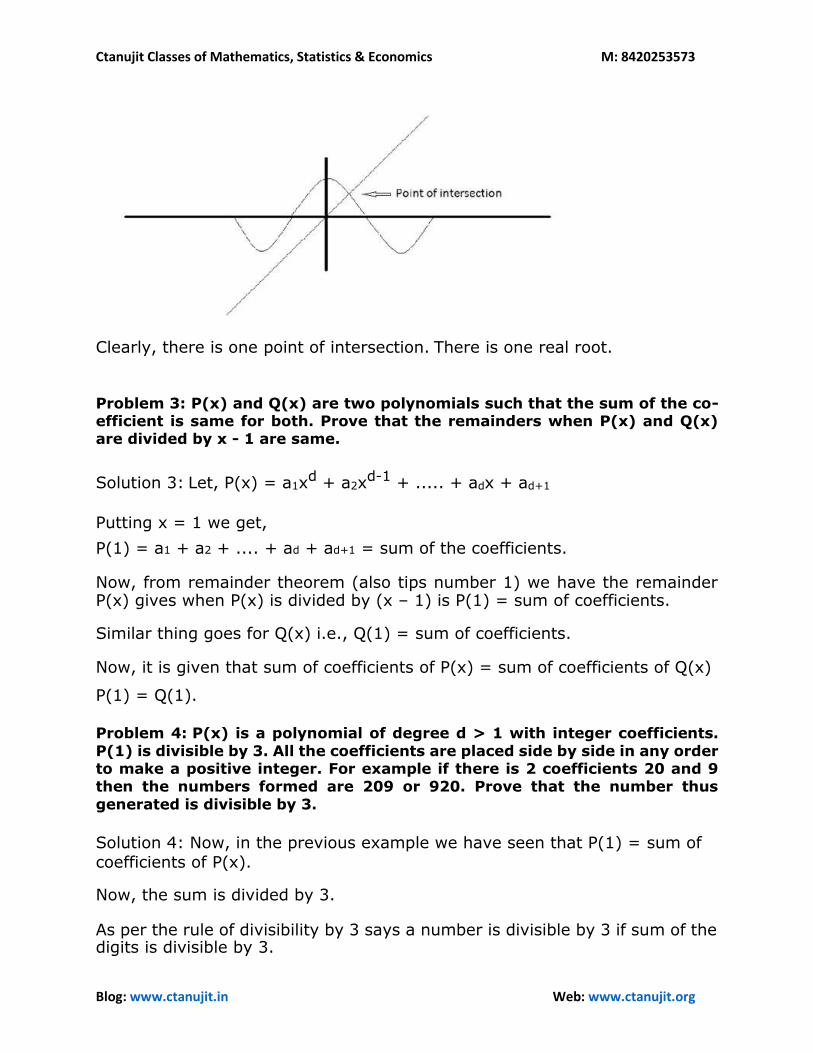
Ctanujit Classes of Mathematics, Statistics & Economics M: 8420253573
Blog: www.ctanujit.in Web: www.ctanujit.org
Clearly, there is one point of intersection. There is one real root.
Problem 3: P(x) and Q(x) are two polynomials such that the sum of the co-efficient is same for both. Prove that the remainders when P(x) and Q(x) are divided by x - 1 are same.
Solution 3: Let, P(x) = a1xd + a2x
d-1 + ..... + adx + ad+1
Putting x = 1 we get, P(1) = a1 + a2 + .... + ad + ad+1 = sum of the coefficients. Now, from remainder theorem (also tips number 1) we have the remainder P(x) gives when P(x) is divided by (x – 1) is P(1) = sum of coefficients.
Similar thing goes for Q(x) i.e., Q(1) = sum of coefficients.
Now, it is given that sum of coefficients of P(x) = sum of coefficients of Q(x) P(1) = Q(1).
Problem 4: P(x) is a polynomial of degree d > 1 with integer coefficients.
P(1) is divisible by 3. All the coefficients are placed side by side in any order to make a positive integer. For example if there is 2 coefficients 20 and 9 then the numbers formed are 209 or 920. Prove that the number thus
generated is divisible by 3.
Solution 4: Now, in the previous example we have seen that P(1) = sum of
coefficients of P(x).
Now, the sum is divided by 3. As per the rule of divisibility by 3 says a number is divisible by 3 if sum of the digits is divisible by 3.
Ctanujit Classes of Mathematics, Statistics & Economics M: 8420253573
Blog: www.ctanujit.in Web: www.ctanujit.org
The sum of the digits of the coefficients of P(x) is divisible by 3.
Now, whatever be the order of placing the digits of the coefficients of P(x) the sum of their digits must be same. The sum of the digits is divisible by 3.
Thus the number generated with whatever be the order of placing the digits is divisible by 3.
Problem 5: Show that the equation x(x - 1)(x - 2).....(x - 2009) = c has real
roots of multiplicity at most 2.
Solution 7: (tips number 11)
As per the tips we need to show P‟‟(x) doesn’t have the root which P(x) and P‟(x) has.
We have, x(x - 1)(x - 2).....(x - 2009) = c
Differentiating w.r.t. x we get, (x – 1)(x – 2)....(x – 2009) + x(x – 2)(x – 3)....(x – 2009) + x(x – 1)(x – 3)...(x – 2009) + ..... + x(x – 1)(x – 2)....(x – 2008) = 0
c/x + c/(x – 1) + c/(x – 2) + .... + c/(x – 2009) = 0
(Putting value from the given equation)
c{1/x + 1/(x – 1) + 1/(x – 2) + .... + 1/(x – 2009)} = 0
Now, differentiating again w.r.t. x we get,
-c × {1/x2 + 1/(x – 1)2 + 1/(x – 2)2 + .... + 1/(x – 2009)2} = 0 This equation cannot hold true as sum of squares of real numbers equal to 0 but they are always greater than 0.
The given polynomial cannot have real roots of multiplicity more than 2.
Problem 6: Prove that the polynomial P(x) = x3 + x – 2 have at least one real root.
Solution 8: (Tips number 10)
Let all the roots of P(x) is complex.
Ctanujit Classes of Mathematics, Statistics & Economics M: 8420253573
Blog: www.ctanujit.in Web: www.ctanujit.org
Complex roots come in pair.
There needs to be 4 roots of P(x)
But P(x) have at most 3 roots as the degree of the polynomial is 3.
Our assumption was wrong. It may have at most 2 complex root.
There is at least one real root of P(x).
Solved examples:
1. Consider a polynomial P(x) of degree d > 1. Q(x) is the quotient when
P(x) is divided by x - a. Prove that P'(a) = Limiting value of Q(x) as x -> a.
Solution: We can write, P(x) = (x – a)Q(x) + R(x) where R(x) is remainder when P(x) is divided by (x – a).
R(x) is constant.
Now, P‟(a) = {P(x) – P(a)}/(x – a) as x -> a P‟(a) = {(x – a)Q(x) + R(x) – R(a)}/(x – a) as x -> a (P(a) = R(a))
P‟(a) = Q(x) as x -> a + {R(x) – R(a)}/(x – a) as x -> a
P‟(a) = Q(x) as x -> a + R‟(a)
P‟(a) = Q(x) as x -> a (as R‟(a) = 0 because R(x) is constant)
2. Consider a polynomial P(x) of degree d > 2. Let R(x) be the remainder when P(x) is divided by (x - 1)2. P'(1) = P(1) = 1. Find R(x).
Solution: We can write, P(x) = (x – 1)2Q(x) + R(x) where Q(x) is the
quotient when P(x) is divided by (x – 1)2. P‟(x) = 2(x – 1)Q(x) + (x – 1)2Q‟(x) + R‟(x) P‟(1) = R‟(1) = 1
And, P(1) = R(1) = 1
Now, R(x) is remainder when P(x) is divided by (x – 1)2
R(x) is linear. Say, R(x) = ax + b
Now, R‟(x) = a
R‟(1) = a = 1
Now, R(1) = a + b = 1
Ctanujit Classes of Mathematics, Statistics & Economics M: 8420253573
Blog: www.ctanujit.in Web: www.ctanujit.org
b = 0. So,
R(x) = x.
3. Let P(x) be a polynomial of degree d > 2. Q(x) is the quotient when P(x) is divided by (x - 2)2. Q(2) = 4. Find P''(2).
Solution: We can write, P(x) = (x – 2)2Q(x) + R(x) where R(x) is remainder
when P(x) is divided by (x – 2)2. So, R(x) is linear.
Now, P‟(x) = 2(x – 2)Q(x) + (x – 2)2Q‟(x) + R‟(x) P‟(x) = 2Q(x) + 2(x – 2)Q‟(x) + 2(x – 2)Q‟(x) + (x – 2)2Q‟(x) + R‟(x)
P‟(2) = 2Q(2) + R‟‟(2) Now, R‟(2) = 0 as R(x) is linear. P‟(2) = 2Q(2) = 2×4 = 8.
4. P(x) and Q(x) are two polynomials such that the sum of the coefficient is
same for both. Prove that the remainders when P(x) and Q(x) are divided by x - 1 are same.
Solution: Sum of the coefficients of P(x) and Q(x) are same.
P(1) = Q(1).
Now, as per Remainder theorem P(1) and Q(1) are remainders when P(x) and Q(x) are divided by (x – 1) and they are clearly same.
5. P(x) is a polynomial of degree d > 1 with integer coefficients. P(1) is divisible by 3. All the coefficients are placed side by side in any order to make a positive integer. For example if there is 2 coefficients 20 and 9 then the numbers formed are 209 or 920. Prove that the number thus generated is divisible by 3.
Solution: P(1) is divisible by 3.
Sum of the coefficients is divisible by 3.
If we place the coefficients side by side then the number formed will be divisible by 3 as the sum of the digits is divisible by 3 as per P(1) is
Ctanujit Classes of Mathematics, Statistics & Economics M: 8420253573
Blog: www.ctanujit.in Web: www.ctanujit.org
divisible by 3.
6. Consider a polynomial P(x) of degree d > 2. Q(x) is the quotient when P(x) is divided by D(x). D(x) is quadratic and x = a is a root. P''(a) = b and Q(a) = b/2. Prove that D(x) has repeated root at x = a.
Solution: Let, D(x) = (x – a)(x – d) We can write, P(x) = D(x)Q(x) + R(x) where R(x) is remainder when P(x) is divided by D(x). R(x) is linear as D(x) is quadratic.
P(x) = (x – a)(x – d)Q(x) + R(x)
P‟(x) = (x – d)Q(x) + (x – a)Q(x) + (x – a)(x – d)Q‟(x) + R‟(x)
P‟‟(x) = Q(x) + (x – d)Q‟(x) + Q(x) + (x – a)Q‟(x) + (x – d)Q‟(x) + (x – a)Q‟(x) + (x – c)(x – d)Q‟(x) + R‟(x)
P‟(a) = 2Q(a) + 2(a – d)Q‟(a) + R‟(a)
b = 2(b/2) + 2(a – d)Q‟(a) (R‟‟(a) = 0 as R(x) is linear)
(a – d)Q‟(a) = 0
d = a
D(x) has repeated root at x = a.
7. Consider two polynomials P(x) and Q(x) of degree d > 0 with integer coefficients. P(0) = Q(0). Prove that there exists an integer n which divides both P(n) and Q(n).
Solution: P(0) = Q(0) The constant term of P(x) and Q(x) are equal. Let,
P(x) = a1xp + a2xp – 1 + ….. + apx + n
Let, Q(x) = b1xq + b2xq – 1+ …..+bqx +n
Clearly n divides both P(n) and Q(n).
8. Let P(x) be a polynomial of degree 3d - 1 where d > 0.
Let P(i)(0) = 3×(i!) where P(i)(x) is i-th derivative of P(x) w.r.t. x. Prove that P(1) is divisible by 9.
Solution:
P(x) = a1xn + a2xn-1 + …. + an-1x2 + anx + an+1 P(0)
= an+1 = 3 P‟(0) = an = 3
P‟(0) = (2!)an-1 = 3×2!
Ctanujit Classes of Mathematics, Statistics & Economics M: 8420253573
Blog: www.ctanujit.in Web: www.ctanujit.org
an-1 = 3.
Similarly, an-2 = an-3 = …. = a1 = 3.
Now, P(1) = a1 + a2 + … + an+1 = a1 + a2 + …. + a3d as n = 3d – 1. P(1) = 3 + 3 + …. 3d times. = 3×3d = 9d
P(1) is divisible by 9.
9. Consider a polynomial P(x) of degree d > 1. Given P(0) = 25. All the roots
of P(x) are distinct positive integers. P(d)(0) = d! . Find the value of P(d-
1)(0)/(d-1)! where P(m)(x) is m-th derivative of P(x) w.r.t. x.
Solution:
Let, P(x) = a1xd + a2xd-1 + …… + ad-1x2 + adx + 25 (As P(0) = 25) Now, P‟(0) = ad = 1
P‟(0) = (2!)ad-1 = 2!
ad-1 = 1
Similarly ad-2 = ad-3 = ad-4 = …. = a2 = a1 = 1
Now, P(d-1)(0) = (d – 1)!×a2
P(d-1)(0)/(d–1)! = a2= 1
10. Let P(x) and Q(x) be two polynomials of degree d1 and d2 respectively where d1 and d2 are both odd. Prove that the sum of the squares of the number of real roots of P(x) and Q(x) cannot be equal to an where a and n are positive integers, n > 1.
Solution: Now, if P(x) have complex roots then they will come in pair (complex + conjugate)
So, number of real roots of P(x) must be odd as degree = d1 = odd.
Similarly, number of real roots of Q(x) must be odd. Let, number of real roots of P(x) and Q(x) are u and v respectively.
Now, let, u2 + v2 = an
As u and v are both odd, a is even.
Now, dividing the equation by 4 we get,
1 + 1 ≡ 0 (mod 4) as n > 1
Ctanujit Classes of Mathematics, Statistics & Economics M: 8420253573
Blog: www.ctanujit.in Web: www.ctanujit.org
2 ≡ 0 (mod 4)
Which is impossible Sum of squares of the number of real roots of P(x) and Q(x) cannot be equal to an where a and n are positive integers, n > 1.
10. Let a, b, c be three distinct integers, and let P be a polynomial with integer coefficients. Show that in this case the conditions P(a) = b, P(b) = c, P(c) = a cannot be satisfied simultaneously.
Solution:
Suppose the conditions are satisfied. We derive a contradiction.
P(x) – b = (x − a)P1(x) ……………… (1)
P(x) – c = (x − b)P2(x) ……………… (2)
P(x) – a = (x − c)P3(x) ……………… (3) Among the numbers a, b, c, we choose the pair with maximal absolute difference.
Suppose this is |a − c|. Then we have
|a − b| < |a − c|……………………. (4)
If we replace x by c in (1), then we get
a – b = (c − a)P1(c).
Since P1(c) is an integer, we have |a − b| ≥ |c − a|, which contradicts
(4).
12. Let f(x) be a monic polynomial with integral coefficients. If there are four different integers a, b, c, d, so that f(a) = f(b) = f(c) = f(d) = 5, then there is no integer k, so that f(k) = 8.
Solution: Monic polynomial means the highest degree coefficient is 1.
Now, f(x) = (x – a)(x – b)(x – c)(x – d)Q(x) + 5
Now, f(k) = (k – a)(k – b)(k – c)(k – d)Q(k) + 5
(k – a)(k – b)(k – c)(k – d)Q(k) = 3 (As f(k) = 8)
3 is factor of at least four distinct integers k – a, k – b, k – c, k – d as a, b, c, d are distinct.
Ctanujit Classes of Mathematics, Statistics & Economics M: 8420253573
Blog: www.ctanujit.in Web: www.ctanujit.org
But this is impossible as 3 is prime and may have maximum 3 factors viz. 3, 1, -1.
Problem: Check whether n68 + n37 + 1 is divisible by n2 + n + 1.
Solution: As ω is cube root of unity so we have ω2 + ω + 1 = 0 and
ω3 = 1.
Put ω in place of n and check whether the given expression is divisible by ω2
+ ω + 1 or not. This is possible because n3 ≡ 1 (mod n2 + n + 1)
So, n68 + n37 + 1 = ω68 + ω37 + 1 = ω2 + ω + 1 = 0
Hence, n2 + n + 1 divides n68 + n37 + 1.
How to solve the questions like “how many real solutions does this
equation have?” and you have a four-degree equation. 1. First check if you can factorize using Vanishing method with 1, 2,
- 1, -2, maximum verify by 3. 2. Then check the degree of the equation. If it is odd then it has at least one
real solution. If it is even then it may have no real solution at all because complex roots come in pair.
3. Then use Descartes‟ sign rule to evaluate if there is any positive or negative real roots. Descartes‟ sign rule says: check number of sign changes of the coefficients from higher degree to lower degree of the polynomial and that says number of maximum possible positive roots of the equation. If it has 4 sign changes then it may have 4 or 2 or 0 number of positive roots i.e. it comes down by an even number 2. Check of negative roots is my same method but of the polynomial P(-x). So, put x = -x and then find number of negative roots of the equation. If there is no then all roots are complex, otherwise it may have real roots.
4. Check whether the polynomial is increasing or decreasing for some value of x. For example, it is a fourth degree equation and we have evaluated that it may have 4 positive roots. And you see the polynomial is increasing for x > 0. Implies the polynomial doesn’t meet the x-axis after x > 0. Therefore, all the roots it has negative but from Descartes‟ sign rule we have zero negative roots. Implies all the roots of the equation are complex.
5. Take any complex root of the equation as a + ib, then a – ib is also a root of the equation. Now, do P(a + ib) – P(a – ib) = 0 and check whether b = 0 for sure. If it comes out to be b = 0, then it has no imaginary roots as the imaginary part of the root is zero.
Ctanujit Classes of Mathematics, Statistics & Economics M: 8420253573
Blog: www.ctanujit.in Web: www.ctanujit.org
Problem: The number of real roots of x5 + 2x3 + x2 + 2 = 0
Solution: First check x = -1 is a solution. So, we will first factorize it by vanishing method.
Now, x5 + 2x3 + x2 + 2
= x5 + x4 – x4 – x3 + 3x3 + 3x2 – 2x2 – 2x + 2x + 2
= x4(x + 1) – x3(x + 1) + 3x2(x + 1) – 2x(x + 1) + 2(x + 1)
= (x + 1)(x4 – x3 + 3x2 – 2x + 2) It is a fifth degree equation and we have evaluated one real root x = -1.
Now, we have a four degree equation, x4 – x3 + 3x2 – 2x + 2 = 0 Number of sign change = 4. Therefore, it may have 4, 2 or 0 positive roots. And it has 0 negative roots.
P(x) = x4 – x3 + 3x2 – 2x + 2 P(0) = 2, P(1) = 3, P(2) = 18 and we are seeing that it is increasing with
(+)-ve value of x.
So, P‟(x) = 4x3 – 3x2 +3x – 2
= x(4x2 – 4x + 1) + (x2 + 2x – 2)
= x(2x – 1)2 + (x – 1)(x + 2) + x > 0 for x > 2
P(x) is increasing for x > 2.
P(x) may have negative real roots but from Descartes‟ sign rule it has no negative roots.
All the roots of the four degree equation are complex.
The equation has only one real root and that is x = -1.
Ctanujit Classes of Mathematics, Statistics & Economics M: 8420253573
Blog: www.ctanujit.in Web: www.ctanujit.org
Elements of Combinatorial Probability
RULE –I : If there are two groups G1 & G2;
𝐺1 = {𝑎1, 𝑎2, … . , 𝑎𝑛} consisting of n elements and 𝐺2 = {𝑏1, 𝑏2, … . , 𝑏𝑚} consisting of m elements then
the no. of pairs (𝑎𝑖 , 𝑏𝑗 ) formed by taking one element 𝑎𝑖 𝑓𝑟𝑜𝑚 𝐺1 𝑎𝑛𝑑 𝑏𝑗 𝑓𝑟𝑜𝑚 𝐺2 𝑖𝑠 𝑛 × 𝑚.
If there are k groups 𝐺1, 𝐺2, … . . , 𝐺𝑘, such that
𝐺1 = {𝑎1, 𝑎2, … . . , 𝑎𝑛1}
𝐺2 = {𝑏1, 𝑏2, … . . , 𝑏𝑛2}
⋮
⋮
𝐺𝑘 = {𝑡1, 𝑡2, … . . , 𝑡𝑛𝑘}
Then the number ordered k−tuples (𝑎𝑖1, 𝑏𝑖2, … . . , 𝑡𝑖𝑘) formed by taking one element from each group is
= 𝑛1 × 𝑛2 × ……× 𝑛𝑘
Example: ‘Placing balls into the cells’ amounts to choose one cell for each ball. Let there are r balls and
n cells. For the 1st ball, we can choose any one of the n cells. Similarly, for each of the balls, we have n
choices, assuming the capacity of each cell is infinite or we can place more than one ball in each cell.
Hence the r balls can be placed in the n cells in 𝑛𝑟 ways.
Applications:
1. A die is rolled r times. Find the probability that –
i) No ace turns up.
ii) No ace turns up.
Solution:
i) The experiment of throwing a die r times has 6 × 6 × 6… . 𝑟 𝑡𝑖𝑚𝑒𝑠 = 6𝑟 possible outcomes.
Assume that all possible cases are equally likely. The no. of cases favorable to the event (A), ‘no ace
turns up’ is 5𝑟.
By Classical Definition, 𝑃[𝐴] =𝑁(𝐴)
𝑁=5𝑟
6𝑟.
ii) P[ an ace turns up] = 1 − 𝑃[𝑛𝑜 𝑎𝑐𝑒 𝑡𝑢𝑟𝑛𝑠 𝑢𝑝] = 1 −5𝑟
6𝑟.
Remark : The all possible outcomes of ‘r’ throw of a die correspond to the placing r balls into 𝑛 = 6 cells.
Ctanujit Classes of Mathematics, Statistics & Economics M: 8420253573
Blog: www.ctanujit.in Web: www.ctanujit.org
RULE –II:
Ordered Samples: Consider a population of n elements 𝑎1, 𝑎2, … . 𝑎𝑛 any order arrangement
𝑎𝑗1, 𝑎𝑗2, … . , 𝑎𝑗𝑟 of r elements is called an ordered sample of size r, drawn from the population. Two
procedure are possible –
i) Sampling with replacement: Here an element is selected from the population and the
selected element is returned to the population before the next selection is made. Each
selection is made from the entire population, so that the same element can be drawn more
than ones.
ii) Sampling without replacement : Here an element once chosen is removed from the
population, so that the sample becomes an arrangement without repetition.
For a population with n elements and a prescribed sample size r, there are 𝑛𝑟 different ordered
samples with replacement and n(n−1)…..(n−r+1) = 𝑛𝑝𝑟 𝑜𝑟 (𝑛)𝑟 different ordered samples
without replacement.
Remark:
1. 𝑛𝑝𝑟 = 𝑛(𝑛 − 1)… . (𝑛 − 𝑟 + 1) is defined if 𝑛 ∈ 𝑁 and r is a non−negative integers. But (𝑛)𝑟 =
𝑛(𝑛 − 1)… . (𝑛 − 𝑟 + 1) is defined if 𝑛 ∈ 𝑅 and r is non−negative integer. In the same way if
𝑛 ∈ ℝ then
𝑛𝑐𝑅 = (𝑛
𝑟) =
𝑛(𝑛 − 1)…… . (𝑛 − 𝑟 + 1)
𝑟!
Example : 1) A random sample of size ‘r’ with replacement is taken from a population of n elements.
Find the probability that in the sample no element appear twice.
Solution: There are 𝑛𝑟 sample in all. As the samples are drawn randomly, all samples are equally likely.
The no. of the samples in which in which no element appears twice is the no. of samples drawn without
replacement.
Favorable sample is = 𝑛(𝑛 − 1)… . (𝑛 − 𝑟 + 1) = (𝑛)𝑟
Hence, the probability is =(𝑛)𝑟
𝑛𝑟
Example: 2) If n balls are randomly placed into n cells, what is the probability that each cell will be
occupied.
Solution: 𝑃(𝐴) =𝑛!
𝑛𝑛.
Ctanujit Classes of Mathematics, Statistics & Economics M: 8420253573
Blog: www.ctanujit.in Web: www.ctanujit.org
SOLVED EXAMPLES:
1. Find the probability that among five randomly selected digits, all digits are different.
Ans:
𝑃(𝐴) =(10)5105
2. In a city seven accidents occur each week in a particular week there occurs one accidents per
day. Is it surprising?
Ans :
𝑃(𝐴) =7!
77
3. An elevator (lift) stands with 7 passengers and stops at 10th floor. What is the probability that
no two passengers leave at the same floor?
Solution:
𝑁 = 10,10… . .10 (7 𝑡𝑖𝑚𝑒𝑠)
= 107
𝑁(𝐴) = 10.9.8.7.6.5.4
= (10)7
𝑃(𝐴) =(10)7107
4. What is the probability that r individuals have different birthdays? Also show that the
probability is approximately equal to 𝒆−𝒓(𝒓−𝟏)/𝟕𝟑𝟎. How many people are required to make
the prob. of distinct birthdays less than ½ ?
Solution:
𝑝 =(365)𝑟365𝑟
=365.364…… . (365 − 𝑟 + 1)
365.365………… . .365
= 1(1 −1
365) (1 −
2
365)……(1 −
𝑟 − 1
365)
∴ ln 𝑝 = ∑ ln(1 −𝑘
365)
𝑟−1
𝑘=1
𝐹𝑜𝑟, 0 < 𝑥 < 1, ln(1 − 𝑥) ≅ −𝑥.
Ctanujit Classes of Mathematics, Statistics & Economics M: 8420253573
Blog: www.ctanujit.in Web: www.ctanujit.org
∴ ln 𝑝 ≅ ∑(−𝑘
365) = −
1
365(∑𝑘
𝑟−1
𝑘=1
)
𝑟−1
𝑘=1
= −𝑟(𝑟 − 1)
2(365) = –
𝑟(𝑟 − 1)
730
∴ 𝑝 = 𝑒−𝑟(𝑟−1)/730
𝐹𝑜𝑟 𝑝 =1
2, ln 𝑝 = − ln 2 = −0.693,
∴𝑟(𝑟 − 1)
730= 0.693
∴ 𝑟2 − 𝑟 − 506 = 0
⇒ (𝑟 − 23)(𝑟 + 22) = 0
⇒ 𝑟 = 23
∴ More than 23 people are required.
5. Six dice are thrown. What’s the prob. that every possible number will appear.
Hints: 𝑝 =6!
66 = 0.0154
6. There are four children in a family. Find the prob. that
(a) At least two of them have the same birthday?
(b) Only the oldest and the youngest have the same birthday?
Hints: (a)
𝑝1 = 1 − {(365)43654
} = 1 − 𝑝 {𝑡ℎ𝑒𝑚 ℎ𝑎𝑣𝑒 𝑑𝑖𝑓𝑓𝑒𝑟𝑒𝑛𝑡 𝑏𝑖𝑟𝑡ℎ𝑑𝑎𝑦𝑠}
(b)
𝑝2 =365 × 365 × 363
3654 =(365)33654
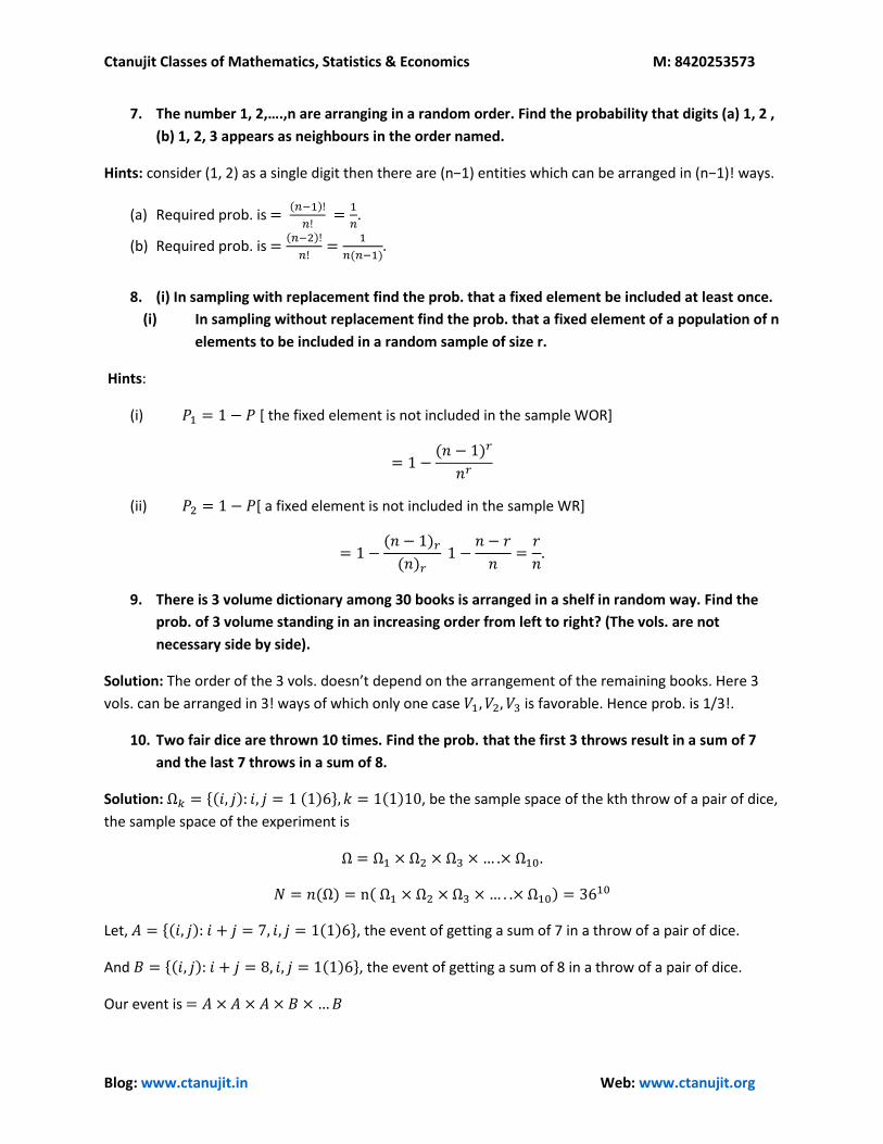
Ctanujit Classes of Mathematics, Statistics & Economics M: 8420253573
Blog: www.ctanujit.in Web: www.ctanujit.org
7. The number 1, 2,….,n are arranging in a random order. Find the probability that digits (a) 1, 2 ,
(b) 1, 2, 3 appears as neighbours in the order named.
Hints: consider (1, 2) as a single digit then there are (n−1) entities which can be arranged in (n−1)! ways.
(a) Required prob. is = (𝑛−1)!
𝑛! =
1
𝑛.
(b) Required prob. is =(𝑛−2)!
𝑛!=
1
𝑛(𝑛−1).
8. (i) In sampling with replacement find the prob. that a fixed element be included at least once.
(i) In sampling without replacement find the prob. that a fixed element of a population of n
elements to be included in a random sample of size r.
Hints:
(i) 𝑃1 = 1 − 𝑃 [ the fixed element is not included in the sample WOR]
= 1 −(𝑛 − 1)𝑟
𝑛𝑟
(ii) 𝑃2 = 1 − 𝑃[ a fixed element is not included in the sample WR]
= 1 −(𝑛 − 1)𝑟(𝑛)𝑟
1 −𝑛 − 𝑟
𝑛=𝑟
𝑛.
9. There is 3 volume dictionary among 30 books is arranged in a shelf in random way. Find the
prob. of 3 volume standing in an increasing order from left to right? (The vols. are not
necessary side by side).
Solution: The order of the 3 vols. doesn’t depend on the arrangement of the remaining books. Here 3
vols. can be arranged in 3! ways of which only one case 𝑉1, 𝑉2, 𝑉3 is favorable. Hence prob. is 1/3!.
10. Two fair dice are thrown 10 times. Find the prob. that the first 3 throws result in a sum of 7
and the last 7 throws in a sum of 8.
Solution: Ω𝑘 = {(𝑖, 𝑗): 𝑖, 𝑗 = 1 (1)6}, 𝑘 = 1(1)10, be the sample space of the kth throw of a pair of dice,
the sample space of the experiment is
Ω = Ω1 × Ω2 × Ω3 × … .× Ω10.
𝑁 = 𝑛(Ω) = n( Ω1 × Ω2 × Ω3 × … . .× Ω10) = 3610
Let, 𝐴 = {(𝑖, 𝑗): 𝑖 + 𝑗 = 7, 𝑖, 𝑗 = 1(1)6}, the event of getting a sum of 7 in a throw of a pair of dice.
And 𝐵 = {(𝑖, 𝑗): 𝑖 + 𝑗 = 8, 𝑖, 𝑗 = 1(1)6}, the event of getting a sum of 8 in a throw of a pair of dice.
Our event is = 𝐴 × 𝐴 × 𝐴 × 𝐵 × …𝐵
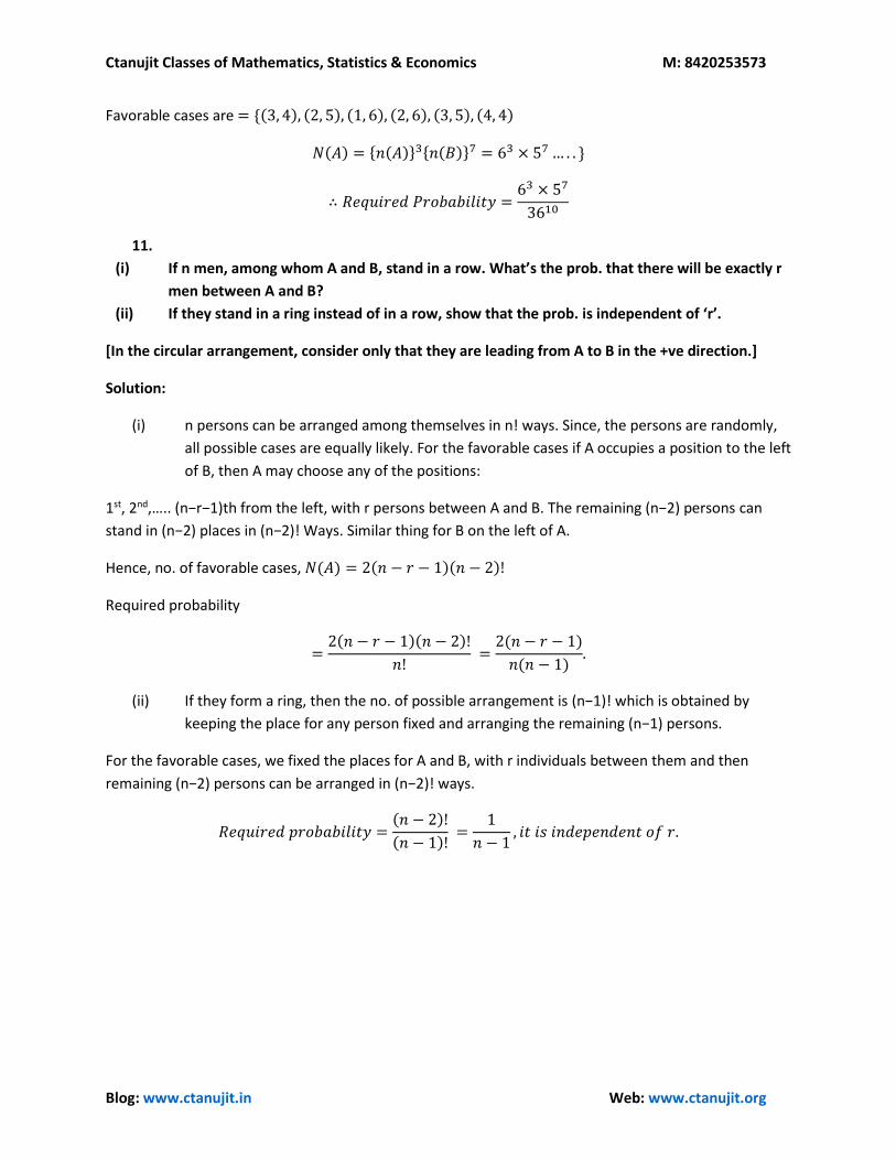
Ctanujit Classes of Mathematics, Statistics & Economics M: 8420253573
Blog: www.ctanujit.in Web: www.ctanujit.org
Favorable cases are = {(3, 4), (2, 5), (1, 6), (2, 6), (3, 5), (4, 4)
𝑁(𝐴) = {𝑛(𝐴)}3{𝑛(𝐵)}7 = 63 × 57… . . }
∴ 𝑅𝑒𝑞𝑢𝑖𝑟𝑒𝑑 𝑃𝑟𝑜𝑏𝑎𝑏𝑖𝑙𝑖𝑡𝑦 =63 × 57
3610
11.
(i) If n men, among whom A and B, stand in a row. What’s the prob. that there will be exactly r
men between A and B?
(ii) If they stand in a ring instead of in a row, show that the prob. is independent of ‘r’.
[In the circular arrangement, consider only that they are leading from A to B in the +ve direction.]
Solution:
(i) n persons can be arranged among themselves in n! ways. Since, the persons are randomly,
all possible cases are equally likely. For the favorable cases if A occupies a position to the left
of B, then A may choose any of the positions:
1st, 2nd,….. (n−r−1)th from the left, with r persons between A and B. The remaining (n−2) persons can
stand in (n−2) places in (n−2)! Ways. Similar thing for B on the left of A.
Hence, no. of favorable cases, 𝑁(𝐴) = 2(𝑛 − 𝑟 − 1)(𝑛 − 2)!
Required probability
=2(𝑛 − 𝑟 − 1)(𝑛 − 2)!
𝑛! =2(𝑛 − 𝑟 − 1)
𝑛(𝑛 − 1).
(ii) If they form a ring, then the no. of possible arrangement is (n−1)! which is obtained by
keeping the place for any person fixed and arranging the remaining (n−1) persons.
For the favorable cases, we fixed the places for A and B, with r individuals between them and then
remaining (n−2) persons can be arranged in (n−2)! ways.
𝑅𝑒𝑞𝑢𝑖𝑟𝑒𝑑 𝑝𝑟𝑜𝑏𝑎𝑏𝑖𝑙𝑖𝑡𝑦 =(𝑛 − 2)!
(𝑛 − 1)! =
1
𝑛 − 1, 𝑖𝑡 𝑖𝑠 𝑖𝑛𝑑𝑒𝑝𝑒𝑛𝑑𝑒𝑛𝑡 𝑜𝑓 𝑟.
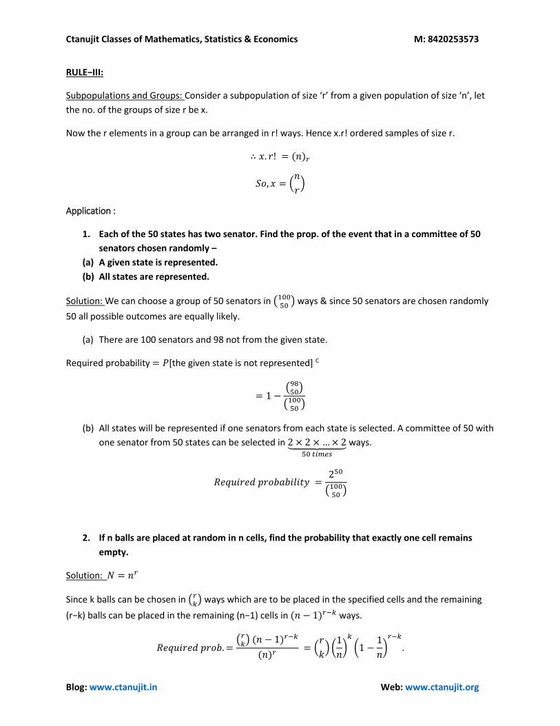
Ctanujit Classes of Mathematics, Statistics & Economics M: 8420253573
Blog: www.ctanujit.in Web: www.ctanujit.org
RULE−III:
Subpopulations and Groups: Consider a subpopulation of size ‘r’ from a given population of size ‘n’, let
the no. of the groups of size r be x.
Now the r elements in a group can be arranged in r! ways. Hence x.r! ordered samples of size r.
∴ 𝑥. 𝑟! = (𝑛)𝑟
𝑆𝑜, 𝑥 = (𝑛
𝑟)
Application :
1. Each of the 50 states has two senator. Find the prop. of the event that in a committee of 50
senators chosen randomly –
(a) A given state is represented.
(b) All states are represented.
Solution: We can choose a group of 50 senators in (10050) ways & since 50 senators are chosen randomly
50 all possible outcomes are equally likely.
(a) There are 100 senators and 98 not from the given state.
Required probability = 𝑃[the given state is not represented] C
= 1 −(9850)
(10050)
(b) All states will be represented if one senators from each state is selected. A committee of 50 with
one senator from 50 states can be selected in 2 × 2 × …× 2⏟ 50 𝑡𝑖𝑚𝑒𝑠
ways.
𝑅𝑒𝑞𝑢𝑖𝑟𝑒𝑑 𝑝𝑟𝑜𝑏𝑎𝑏𝑖𝑙𝑖𝑡𝑦 =250
(10050)
2. If n balls are placed at random in n cells, find the probability that exactly one cell remains
empty.
Solution: 𝑁 = 𝑛𝑟
Since k balls can be chosen in (𝑟𝑘) ways which are to be placed in the specified cells and the remaining
(r−k) balls can be placed in the remaining (n−1) cells in (𝑛 − 1)𝑟−𝑘 ways.
𝑅𝑒𝑞𝑢𝑖𝑟𝑒𝑑 𝑝𝑟𝑜𝑏.=(𝑟𝑘) (𝑛 − 1)𝑟−𝑘
(𝑛)𝑟 = (
𝑟
𝑘) (1
𝑛)𝑘
(1 −1
𝑛)𝑟−𝑘
.
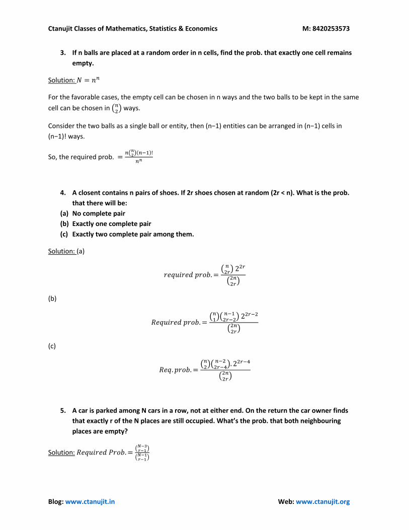
Ctanujit Classes of Mathematics, Statistics & Economics M: 8420253573
Blog: www.ctanujit.in Web: www.ctanujit.org
3. If n balls are placed at a random order in n cells, find the prob. that exactly one cell remains
empty.
Solution: 𝑁 = 𝑛𝑛
For the favorable cases, the empty cell can be chosen in n ways and the two balls to be kept in the same
cell can be chosen in (𝑛2) ways.
Consider the two balls as a single ball or entity, then (n−1) entities can be arranged in (n−1) cells in
(n−1)! ways.
So, the required prob. =𝑛(𝑛2)(𝑛−1)!
𝑛𝑛
4. A closent contains n pairs of shoes. If 2r shoes chosen at random (2r < n). What is the prob.
that there will be:
(a) No complete pair
(b) Exactly one complete pair
(c) Exactly two complete pair among them.
Solution: (a)
𝑟𝑒𝑞𝑢𝑖𝑟𝑒𝑑 𝑝𝑟𝑜𝑏.=( 𝑛2𝑟) 22𝑟
(2𝑛2𝑟)
(b)
𝑅𝑒𝑞𝑢𝑖𝑟𝑒𝑑 𝑝𝑟𝑜𝑏.=(𝑛1)( 𝑛−12𝑟−2
) 22𝑟−2
(2𝑛2𝑟)
(c)
𝑅𝑒𝑞. 𝑝𝑟𝑜𝑏.=(𝑛2)( 𝑛−22𝑟−4
). 22𝑟−4
(2𝑛2𝑟)
5. A car is parked among N cars in a row, not at either end. On the return the car owner finds
that exactly r of the N places are still occupied. What’s the prob. that both neighbouring
places are empty?
Solution: 𝑅𝑒𝑞𝑢𝑖𝑟𝑒𝑑 𝑃𝑟𝑜𝑏.=(𝑁−3𝑟−1)
(𝑁−1𝑟−1)
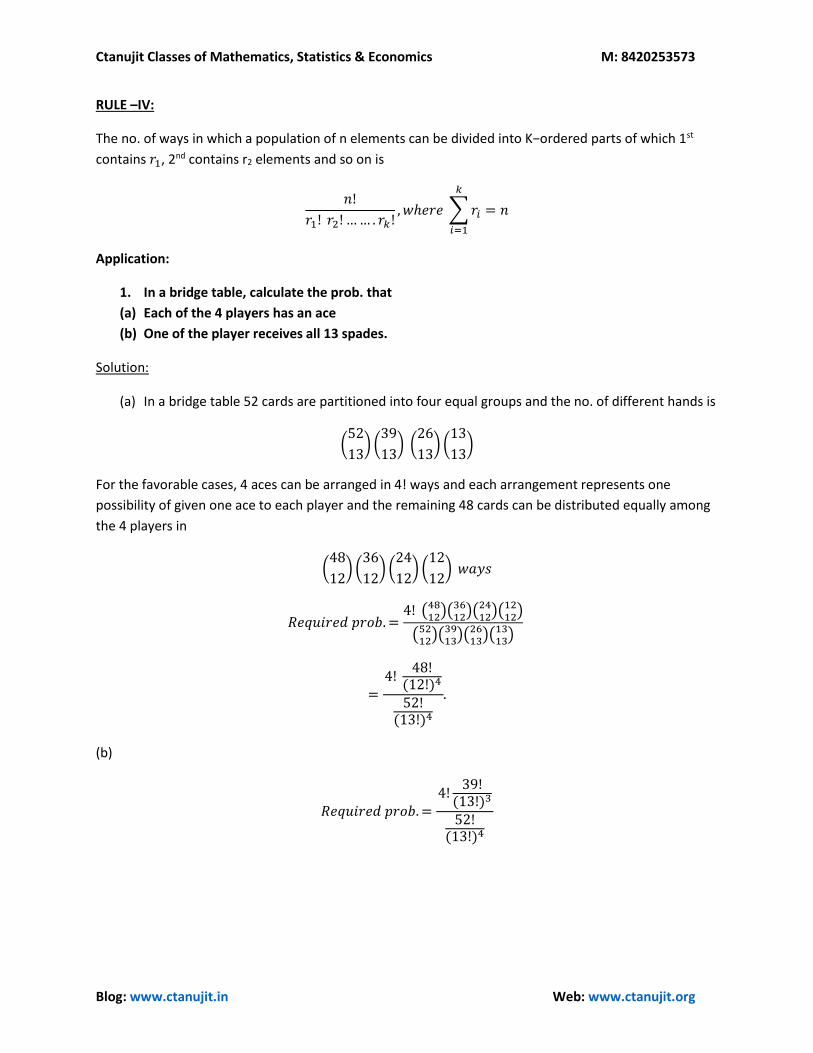
Ctanujit Classes of Mathematics, Statistics & Economics M: 8420253573
Blog: www.ctanujit.in Web: www.ctanujit.org
RULE –IV:
The no. of ways in which a population of n elements can be divided into K−ordered parts of which 1st
contains 𝑟1, 2nd contains r2 elements and so on is
𝑛!
𝑟1! 𝑟2! …… . 𝑟𝑘!, 𝑤ℎ𝑒𝑟𝑒 ∑𝑟𝑖 = 𝑛
𝑘
𝑖=1
Application:
1. In a bridge table, calculate the prob. that
(a) Each of the 4 players has an ace
(b) One of the player receives all 13 spades.
Solution:
(a) In a bridge table 52 cards are partitioned into four equal groups and the no. of different hands is
(52
13) (39
13) (26
13) (13
13)
For the favorable cases, 4 aces can be arranged in 4! ways and each arrangement represents one
possibility of given one ace to each player and the remaining 48 cards can be distributed equally among
the 4 players in
(48
12) (36
12) (24
12) (12
12) 𝑤𝑎𝑦𝑠
𝑅𝑒𝑞𝑢𝑖𝑟𝑒𝑑 𝑝𝑟𝑜𝑏.=4! (48
12)(3612)(2412)(1212)
(5212)(3913)(2613)(1313)
=4!
48!(12!)4
52!(13!)4
.
(b)
𝑅𝑒𝑞𝑢𝑖𝑟𝑒𝑑 𝑝𝑟𝑜𝑏.=4!
39!(13!)3
52!(13!)4
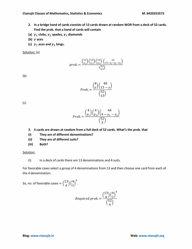
Ctanujit Classes of Mathematics, Statistics & Economics M: 8420253573
Blog: www.ctanujit.in Web: www.ctanujit.org
2. In a bridge hand of cards consists of 13 cards drawn at random WOR from a deck of 52 cards.
Find the prob. that a hand of cards will contain
(a) 𝜸𝟏 clubs, 𝜸𝟐 spades, 𝜸𝟑 diamonds
(b) 𝜸 aces
(c) 𝜸𝟏 aces and 𝜸𝟐 kings.
Solution: (a)
𝑝𝑟𝑜𝑏.=(13𝛾1) (13
𝛾2) (13
𝛾3) ( 13
13−𝛾1−𝛾2−𝛾3)
(5213)
(b)
𝑃𝑟𝑜𝑏.=(4𝛾) (
4813 − 𝛾
)
(5213)
(c)
𝑃𝑟𝑜𝑏.=(4𝛾1) (4𝛾2) (
444 − 𝛾1 − 𝛾2
)
(523)
3. 4 cards are drawn at random from a full deck of 52 cards. What’s the prob. that
(i) They are of different denominations?
(ii) They are of different suits?
(iii) Both?
Solution:
(i) In a deck of cards there are 13 denominations and 4 suits.
For favorable cases select a group of 4 denominations from 13 and then choose one card from each of
the 4 denomination.
So, no. of favorable cases = (134) (41)4
.
𝑅𝑒𝑞𝑢𝑖𝑟𝑒𝑑 𝑝𝑟𝑜𝑏.=(134)(41)4
(524)

Ctanujit Classes of Mathematics, Statistics & Economics M: 8420253573
Blog: www.ctanujit.in Web: www.ctanujit.org
(ii)
𝑟𝑒𝑞𝑢𝑖𝑟𝑒𝑑 𝑝𝑟𝑜𝑏.=(131)4
(524)
(iii) For favorable cases, selecting 4 denominations from 13 and then taking one card from the
1st denomination in 4 ways from the 4 suits. Then taking 2nd from the 2nd denomination in 3
ways & so on.
𝑅𝑒𝑞𝑢𝑖𝑟𝑒𝑑 𝑝𝑟𝑜𝑏𝑎𝑏𝑖𝑙𝑖𝑡𝑦 =(134) × 4!
(524)
4. From a deck of 52 cards are drawn successively until an ace appears. What is the prob. that
the 1st ace will appear
(a) At the nth draw,
(b) After the nth draw.
Solution:
(a) For the favourable cases, at the nth draw an ace can occur in 4 ways and the first (n−1) cards are
to be taken from 48 non−ace cards which can be done in (48)𝑛−1 ways.
∴ 𝑅𝑒𝑞𝑢𝑖𝑟𝑒𝑑 𝑝𝑟𝑜𝑏.=4 × (48)𝑛−1(52)𝑛
(b) For the favorable cases, 1st n cards contain no ace.
∴ 𝑅𝑒𝑞 𝑝𝑟𝑜𝑏.=(48)𝑛(52)𝑛
5. (Spread of Rumours) In a town of (n+1) inhabitants, a person tells a rumour to a second
person, who in turn, repeats it to a third person, etc. At each step the receipt of the rumour is
chosen at random from n people available.
(i) Find the prob. that the rumour will be told r times without
(a) Returning to the originator.
(b) Being repeated to any person.
(ii) Do the same problem when at each step the rumour is told by one person to a gathering
of N randomly chosen individuals.
Solution:
(i) Since any person can tell the rumour to any one of the n available persons in n ways, total
possible cases = 𝑛𝑟.
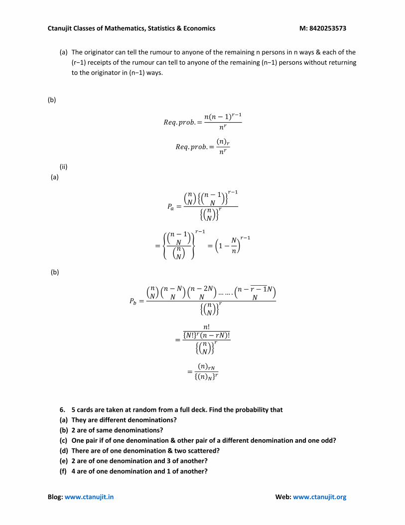
Ctanujit Classes of Mathematics, Statistics & Economics M: 8420253573
Blog: www.ctanujit.in Web: www.ctanujit.org
(a) The originator can tell the rumour to anyone of the remaining n persons in n ways & each of the
(r−1) receipts of the rumour can tell to anyone of the remaining (n−1) persons without returning
to the originator in (n−1) ways.
(b)
𝑅𝑒𝑞. 𝑝𝑟𝑜𝑏.=𝑛(𝑛 − 1)𝑟−1
𝑛𝑟
𝑅𝑒𝑞. 𝑝𝑟𝑜𝑏.=(𝑛)𝑟𝑛𝑟
(ii)
(a)
𝑃𝑎 =(𝑛𝑁) {(
𝑛 − 1𝑁
)}𝑟−1
{(𝑛𝑁)}𝑟
= {(𝑛 − 1𝑁
)
(𝑛𝑁)}
𝑟−1
= (1 −𝑁
𝑛)𝑟−1
(b)
𝑃𝑏 =(𝑛𝑁) (𝑛 − 𝑁𝑁
)(𝑛 − 2𝑁𝑁
)…… . (𝑛 − 𝑟 − 1 𝑁𝑁
)
{(𝑛𝑁)}𝑟
=
𝑛!{𝑁!}𝑟(𝑛 − 𝑟𝑁)!
{(𝑛𝑁)}𝑟
=(𝑛)𝑟𝑁{(𝑛)𝑁}
𝑟
6. 5 cards are taken at random from a full deck. Find the probability that
(a) They are different denominations?
(b) 2 are of same denominations?
(c) One pair if of one denomination & other pair of a different denomination and one odd?
(d) There are of one denomination & two scattered?
(e) 2 are of one denomination and 3 of another?
(f) 4 are of one denomination and 1 of another?
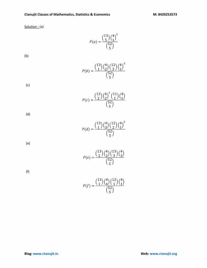
Ctanujit Classes of Mathematics, Statistics & Economics M: 8420253573
Blog: www.ctanujit.in Web: www.ctanujit.org
Solution : (a)
𝑃(𝑎) =(135) (41)5
(525)
(b)
𝑃(𝑏) =(131) (42) (123) (41)3
(525)
(c)
𝑃(𝑐) =(132)(42)2
(111) (41)
(525)
(d)
𝑃(𝑑) =(131) (43) (122)(41)2
(525)
(e)
𝑃(𝑒) =(132) (42) (133)(43)
(525)
(f)
𝑃(𝑓) =(131) (44) (121) (41)
(525)
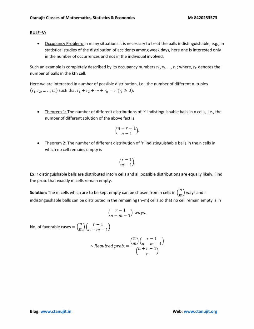
Ctanujit Classes of Mathematics, Statistics & Economics M: 8420253573
Blog: www.ctanujit.in Web: www.ctanujit.org
RULE−V:
Occupancy Problem: In many situations it is necessary to treat the balls indistinguishable, e.g., in
statistical studies of the distribution of accidents among week days, here one is interested only
in the number of occurrences and not in the individual involved.
Such an example is completely described by its occupancy numbers 𝑟1, 𝑟2, … , 𝑟𝑛; where, 𝑟𝑘 denotes the
number of balls in the kth cell.
Here we are interested in number of possible distribution, i.e., the number of different n−tuples
(𝑟1, 𝑟2, … . . , 𝑟𝑛) such that 𝑟1 + 𝑟2 +⋯+ 𝑟𝑛 = 𝑟 (𝑟𝑖 ≥ 0).
Theorem 1: The number of different distributions of ‘r’ indistinguishable balls in n cells, i.e., the
number of different solution of the above fact is
(𝑛 + 𝑟 − 1𝑛 − 1
).
Theorem 2: The number of different distribution of ‘r’ indistinguishable balls in the n cells in
which no cell remains empty is
(𝑟 − 1𝑛 − 1
).
Ex: r distinguishable balls are distributed into n cells and all possible distributions are equally likely. Find
the prob. that exactly m cells remain empty.
Solution: The m cells which are to be kept empty can be chosen from n cells in (𝑛𝑚) ways and r
indistinguishable balls can be distributed in the remaining (n−m) cells so that no cell remain empty is in
(𝑟 − 1
𝑛 −𝑚 − 1) 𝑤𝑎𝑦𝑠.
No. of favorable cases = (𝑛𝑚)(
𝑟 − 1𝑛 −𝑚 − 1
)
∴ 𝑅𝑒𝑞𝑢𝑖𝑟𝑒𝑑 𝑝𝑟𝑜𝑏.=(𝑛𝑚)(
𝑟 − 1𝑛 −𝑚 − 1
)
(𝑛 + 𝑟 − 1
𝑟)
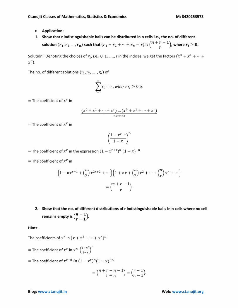
Ctanujit Classes of Mathematics, Statistics & Economics M: 8420253573
Blog: www.ctanujit.in Web: www.ctanujit.org
Application:
1. Show that r indistinguishable balls can be distributed in n cells i.e., the no. of different
solution (𝒓𝟏, 𝒓𝟐, … , 𝒓𝒏) such that {𝒓𝟏 + 𝒓𝟐 +⋯+ 𝒓𝒏 = 𝒓} is (𝒏 + 𝒓 − 𝟏
𝒓), where 𝒓𝒊 ≥ 𝟎.
Solution : Denoting the choices of 𝑟1, i.e., 0, 1, ….., r in the indices, we get the factors (𝑥0 + 𝑥1 +⋯+
𝑥𝑟).
The no. of different solutions (𝑟1, 𝑟2, … . , 𝑟𝑛) of
∑𝑟𝑖 = 𝑟
𝑛
𝑖=1
, 𝑤ℎ𝑒𝑟𝑒 𝑟𝑖 ≥ 0 𝑖𝑠
= The coefficient of 𝑥𝑟 in
(𝑥0 + 𝑥1 +⋯+ 𝑥𝑟)… (𝑥0 + 𝑥1 +⋯+ 𝑥𝑟)⏟ 𝑛 𝑡𝑖𝑚𝑒𝑠
= The coefficient of 𝑥𝑟 in
(1 − 𝑥𝑟+1
1 − 𝑥)
𝑛
= The coefficient of 𝑥𝑟 in the expression (1 − 𝑥𝑟+1)𝑛 (1 − 𝑥)−𝑛
= The coefficient of 𝑥𝑟 in
{1 − 𝑛𝑥𝑟+1 + (𝑛
2)𝑥2𝑟+2 +⋯} {1 + 𝑛𝑥 + (
𝑛
2)𝑥2 +⋯+ (
𝑛
𝑟) 𝑥𝑟 +⋯}
= (𝑛 + 𝑟 − 1
𝑟).
2. Show that the no. of different distributions of r indistinguishable balls in n cells where no cell
remains empty is (𝒏 − 𝟏𝒓 − 𝟏
).
Hints:
The coefficients of 𝑥𝑟 in (𝑥 + 𝑥2 +⋯+ 𝑥𝑟)𝑛
= The coefficient of 𝑥𝑟 in 𝑥𝑛 (1−𝑥𝑟
1−𝑥)𝑛
= The coefficient of 𝑥𝑟−𝑛 𝑖𝑛 (1 − 𝑥𝑟)𝑛(1 − 𝑥)−𝑛
= (𝑛 + 𝑟 − 𝑛 − 1
𝑟 − 𝑛) = (
𝑟 − 1𝑛 − 1
).
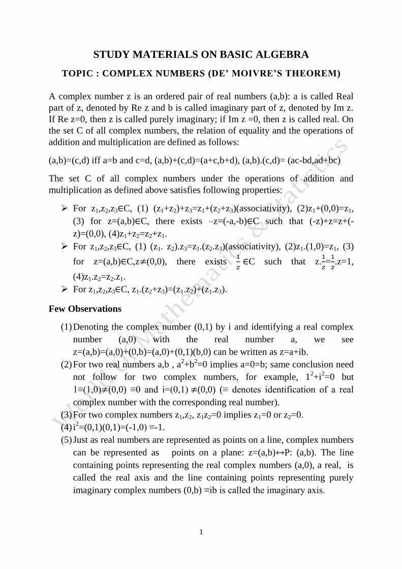
1
STUDY MATERIALS ON BASIC ALGEBRA
TOPIC : COMPLEX NUMBERS (DE’ MOIVRE’S THEOREM)
A complex number z is an ordered pair of real numbers (a,b): a is called Real
part of z, denoted by Re z and b is called imaginary part of z, denoted by Im z.
If Re z=0, then z is called purely imaginary; if Im z =0, then z is called real. On
the set C of all complex numbers, the relation of equality and the operations of
addition and multiplication are defined as follows:
(a,b)=(c,d) iff a=b and c=d, (a,b)+(c,d)=(a+c,b+d), (a,b).(c,d)= (ac-bd,ad+bc)
The set C of all complex numbers under the operations of addition and
multiplication as defined above satisfies following properties:
For z1,z2,z3 C, (1) (z1+z2)+z3=z1+(z2+z3)(associativity), (2)z1+(0,0)=z1,
(3) for z=(a,b) C, there exists –z=(-a,-b) C such that (-z)+z=z+(-
z)=(0,0), (4)z1+z2=z2+z1.
For z1,z2,z3 C, (1) (z1. z2).z3=z1.(z2.z3)(associativity), (2)z1.(1,0)=z1, (3)
for z=(a,b) C,z (0,0), there exists
C such that z.
=
.z=1,
(4)z1.z2=z2.z1.
For z1,z2,z3 C, z1.(z2+z3)=(z1.z2)+(z1.z3).
Few Observations
(1) Denoting the complex number (0,1) by i and identifying a real complex
number (a,0) with the real number a, we see
z=(a,b)=(a,0)+(0,b)=(a,0)+(0,1)(b,0) can be written as z=a+ib.
(2) For two real numbers a,b , a2+b
2=0 implies a=0=b; same conclusion need
not follow for two complex numbers, for example, 12+i
2=0 but
1≡(1,0) (0,0) ≡0 and i=(0,1) (0,0) (≡ denotes identification of a real
complex number with the corresponding real number).
(3) For two complex numbers z1,z2, z1z2=0 implies z1=0 or z2=0.
(4) i2=(0,1)(0,1)=(-1,0) ≡-1.
(5) Just as real numbers are represented as points on a line, complex numbers
can be represented as points on a plane: z=(a,b) P: (a,b). The line
containing points representing the real complex numbers (a,0), a real, is
called the real axis and the line containing points representing purely
imaginary complex numbers (0,b) ≡ib is called the imaginary axis.

2
(6) The plane on which the representation is made is called Gaussian Plane or
Argand Plane.
Definition 1.1 Let z=(a,b) ≡a+ib. The conjugate of z, denoted by , is (a,-b)
≡a-ib.
Geometrically, the point (representing) is the reflection of the point
(representing) z in the real axis. The conjugate operation satisfies the following
properties:
(1) =z , (2) , (3) , (4)(
)
, (4) z+ =2
Rez, z- =2i Im(z)
Definition 1.2 Let z=(a,b) ≡a+ib. The modulus of z, written as | |, is defined as
√ .
Geometrically, | | represents the distance of the point representing z from the
origin (representing complex number (0,0) ≡0+i0). More generally, | | represents the distance between the points z1 and z2. The modulus operation
satisfies the following properties:
(1) | | | | | |, (2) | | | | | | (3) |
|
| |
| |
(4) || | | || | |
GEOMETRICAL REPRESENTATION OF COMPLEX NUMBERS: THE
ARGAND PLANE
Let z=a+ib be a complex number. In the Argand plane, z is represented by the
point whose Cartesian co-ordinates is (a,b) referred to two perpendicular lines
as axes, the first co-ordinate axis is called the real axis and the second the
imaginary axis. Taking the origin as the pole and the real axis as the initial line,
let (r, ) be the polar co-ordinates of the point (a,b). Then a=r cos , b=r sin .
Also r=√ =| |. Thus z=a+ib=| |(cos +isin ): this is called modulus-
amplitude form of z. For a given z 0, there exist infinitely many values of
differing from one another by an integral multiple of 2 : the collection of all
such values of for a given z 0 is denoted by Arg z or Amp z. The principal
value of Arg z , denoted by arg z or amp z, is defined to be the angle from the
collection Arg z that satisfies the condition - . Thus
Arg z={arg z+2n : n an integer}. arg z satisfies following properties:
(1) arg(z1z2)=argz1+argz2+2k , where k is a suitable integer from the set{-1,0,1]
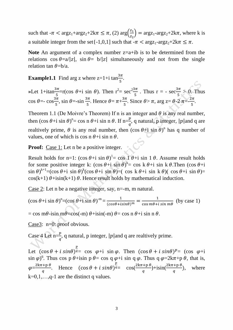
3
such that - argz1+argz2+2k , (2) arg(
) argz1-argz2+2k , where k is
a suitable integer from the set{-1,0,1] such that - argz1-argz2+2k .
Note An argument of a complex number z=a+ib is to be determined from the
relations cos =a/| |, sin = b/| | simultaneously and not from the single
relation tan =b/a.
Example1.1 Find arg z where z=1+i tan
.
»Let 1+itan
=r(cos +i sin ). Then r
2= sec
2
. Thus r = - sec
> 0. Thus
cos =- cos
, sin =-sin
. Hence = +
. Since > , arg z= -2 =-
.
Theorem 1.1 (De Moivre’s Theorem) If n is an integer and is any real number,
then (cos +i sin )n= cos n +i sin n . If n=
, q natural, p integer, | |and q are
realtively prime, is any real number, then (cos +i sin )n has q number of
values, one of which is cos n +i sin n .
Proof: Case 1: Let n be a positive integer.
Result holds for n=1: (cos +i sin )1= cos 1 +i sin 1 . Assume result holds
for some positive integer k: (cos +i sin )k= cos k +i sin k .Then (cos +i
sin )k+1
=(cos +i sin )k(cos +i sin )=( cos k +i sin k )( cos +i sin )=
cos(k+1) +isin(k+1) Hence result holds by mathematical induction.
Case 2: Let n be a negative integer, say, n=-m, m natural.
(cos +i sin )n=(cos +i sin )
-m =
( )
(by case 1)
= cos m -isin m =cos(-m) +isin(-m) = cos n +i sin n .
Case3: n=0: proof obvious.
Case 4 Let n=
, q natural, p integer, | |and q are realtively prime.
Let ( )
= cos +i sin . Then ( ) = (cos +i
sin )q. Thus cos p +isin p = cos q +i sin q . Thus q =2k +p , that is,
=
. Hence ( )
= cos(
)+isin(
), where
k=0,1,…,q-1 are the distinct q values.
4
Some Applications of De’ Moivre’s Theorem
(1) Expansion of cos n , sin n and tan n where n is natural and is real.
Cos n +i sin n =(cos +isin )n=cos
n + cos
n-1 isin + cos
n-
2 +…+insin
n = (cosn -
cosn-2 +…)+i(
cosn-
1 sin - cos
n-3 +…). Equating real and imaginary parts, cos
n = cosn -
cosn-2 +… and sin n =
cosn-1 sin -
cosn-
3 +…
(2) Expansion of cosn and sin
n in a series of multiples of where n is
natural and .
Let x = cos . Then xn=cos n +isin n , x
-n= cos n -isin n .
Thus (2 cos )n=(x+
)n
=(xn+
)
(xn-2
+
)+…=2 cos n +
(2 cos(n-2) )+…
Similarly, expansion of sinn in terms of multiple angle can be derived.
(3) Finding n th roots of unity
To find z satisfying zn=1=cos(2k )+isin(2k ), where k is an integer.
Thus z=[ cos(2k )+isin(2k )]1/n
=cos(
) (
), k=0,1,…,n-1;
replacing k by any integer gives rise to a complex number in the set A={
cos(
) (
)/ k=0,1,…,n-1}. Thus A is the set of all nth roots of
unity.
Example1.2 Solve x6+x
5+x
4+x
3+x
2+x+1=0
»We have the identity x6+x
5+x
4+x
3+x
2+x+1=
. Roots of x
7-1=0 are cos
, k=0,1,…,6. Putting k=0, we obtain root of x-1=0. Thus the roots of
given equation are cos
, k=1,…,6.
5
Example1.3 Prove that the sum of 99 th powers of all the roots of x7-1=0 is
zero.
»The roots of x7-1=0 are {1, , 2
,…, 6}, where =cos
+isin
. Thus sum of
99th powers of the roots is 1+ 99
+( ) ( ) 1+ 99+( )
( ) =
=0, since =1 and 1.
Example1.4 If the amplitude of the complex number
is
, show that z lies
on a circle in the Argand plane.
»Let z=x+iy. Then
=
( )
( ) . By given condition,
=1. On simplification, (x+1)
2+(y-1)
2=1. Hence z lies on the circle
centred at (-1,1) and radius 1.
Example1.5 If A,B,C represent complex numbers z1,z2,z3 in the Argand plane
and z1+z2+z3=0 and | |=| | | |, prove that ABC is an equilateral triangle.
»z1+z2=-z3. Hence | | | |
, that is, | | +| |
+2z1.z2=| | . By
given condition, | || |cos =| | , where is the angle between z1 and
z2.Thus cos =-
, that is, =120
0. Hence the corresponding angle of the triangle
ABC is 600. Similarly other angles are 60
0.
Example1.6 Let z and z1 be two complex numbers satisfying z=
and | |=1.
Prove that z lies on the imaginary axis.
» z1=
. By given condition, |
|
| |
| |. If z=x+iy, x=0. Hence.
Example1.7 complex numbers z1,z2,z3 satisfy the relation z12+z2
2+z3
2-z1z2-z2z3-
z3z1=0 iff | | | | | |.
» 0=z12+z2
2+z3
2-z1z2-z2z3-z3z1=(z1+wz2+w
2z3)(z1+w
2z2+wz3), where w stands for
an imaginary cube roots of unity. If z1+wz2+w2z3=0, then (z1-z2)=-w
2(z3-z2);
hence | |=| || |=| | similarly other part.
6
Conversely, if | | | | | |, then z1,z2,z3 represent vertices
of an equilateral triangle. Then z2-z1=(z3-z1)(cos 600+isin60
0), z1-z2=(z3-z2)( cos
600+isin60
0 ); by dividing respective sides, we get the result.
Example1.8 Prove that | | | |
(| | | |
), for two
complex numbers z1,z2.
| | ( )( )=| |
| | +2 z1z2; similarly |
| =| |
| | -2 z1z2; Adding we get the result.
Example1.9 If cos +cos +cos =sin +sin +sin =0, then prove that (1) cos
3 +cos3 +cos 3 =3cos( + ), (2) ∑ =∑ =3/2.
Let x=cos +i sin , y= cos +i sin , z= cos +i sin . Then x+y+z=0. Thus
x3+y
3+z
3=3xyz. By De’ Moivre’s Theorem, (cos 3 + cos 3 +cos 3 )+i(sin
3 + sin 3 +sin 3 )=3[ cos( )+isin( ) . Equating, we get
result.
Let x=cos +i sin , y= cos +i sin , z= cos +i sin . Then x+y+z=0. Also
hence xy+yz+zx=0. Thus x
2+y
2+z
2=0. By De’ Moivre’s
Theorem, cos 2 +cos2 +cos2 =0. Hence∑ =3/2. Using sin2 =1-
cos2 , we get other part.
Example1.10 Find the roots of zn=(z+1)
n, where n is a positive integer, and
show that the points which represent them in the Argand plane are collinear.
Let w=
Now z
n=(z+1)
n implies w
n=1.Thus, w=cos
,k=0,…,n-1.
So z=
, k=1,…,n-1
=
. Thus all points z satisfying z
n=(z+1)
n lie on the line x=-
.
7
TOPIC : THEORY OF EQUATIONS
An expression of the form a0xn+a1x
n-1+…+an-1x+an, where a0,a1,…,an are real or
complex constants, n is a nonnegative integer and x is a variable (over real or
complex numbers) is a polynomial in x. If a0 0, the polynomial is of degree n
and a0xn is the leading term of the polynomial. A non-zero constant a0 is a
polynomial of degree 0 while a polynomial in which the coefficients of each
term is zero is said to be a zero polynomial and no degree is assigned to a zero
polynomial.
Equality: two polynomials a0xn+a1x
n-1+…+an-1x+an and b0x
n+b1x
n-1+…+bn-
1x+bn are equal iff a0=b0,a1=b1,…,an=bn.
Addition: Let f(x)= a0xn+a1x
n-1+…+an-1x+an, g(x)= b0x
n+b1x
n-1+…+bn-1x+bn.
the sum of the polynomials f(x) and g(x) is given by
f(x)+g(x)= a0xn+…+an-m-1x
m+1+(an-m+b0)x
m+…+(an+bm), if m<n
= (a0+b0)xn+…+(an+bn), if m=n
= b0xm+…+bm-n-1x
n+1+(bm-n+a0)x
n+…+(bm+an), if m>n.
Multiplication: Let f(x)= a0xn+a1x
n-1+…+an-1x+an, g(x)= b0x
n+b1x
n-1+…+bn-
1x+bn. the product of the polynomials f(x) and g(x) is given by
f(x)g(x)=c0xm+n
+c1xm+n-1
+…+cm+n, where ci=a0bi+a1bi-1+…+aib0. c0=a0b0 0;
hence degree of f(x)g(x) is m+n.
Division Algorithm: Let f(x) and g(x) be two polynomials of degree n and m
respectively and n m. Then there exist two uniquely determined polynomials
q(x) and r(x) satisfying f(x)=g(x)q(x)+r(x), where the degree of q(x) is n-m and
r(x) is either a zero polynomial or the degree of r(x) is less than m. In particular,
if degree of g(x) is 1, then r(x) is a constant, identically zero or non-zero.
Theorem 1.1 ( Remainder Theorem)If a polynomial f(x) is divided by x-a,
then the remainder is f(a).
»Let q(x) be the quotient and r (constant)be the remainder when f is divided by
x-a. then f(x)=(x-a)q(x)+r is an identity. Thus f(a)=r.
8
Theorem 1.2 ( Factor Theorem)If f is a polynomial, then x-a is a factor of f
iff f(a)=0.
» By Remainder theorem, f(a) is the remainder when f is divided by x-a; hence,
if f(a)=0, then x-a is a factor of f. Conversely, if x-a is a factor of f, then
f(x)=(x-a)g(x) and hence f(a)=0.
Example1.1 Find the remainder when f(x)=4x5+3x
3+6x
2+5 is divided by 2x+1.
»The remainder on dividing f(x) by x-(-
)=x+
is f(-
)=6. If q(x) be the
quotient, then f(x)=q(x)(x+
)+6=
( )
(2x+1)+6. Hence 6 is the remainder when f
is divided by 2x+1.
Theorem 1.3 ( Fundamental Theorem of Classical Algebra)
Every polynomial equation of degree 1 has a root, real or complex.
Corollary A polynomial equation of degree n has exactly n roots, multiplicity
of each root being taken into account.
Corollary If a polynomial f(x) of degree n vanishes for more than n distinct
values of x, then f(x) =0 for all values of x.
Polynomial equations with Real Coefficients
Theorem 1.4 If a+ib is a root of multiplicity r of the polynomial equation
f(x)=0 with real coefficients, then a-ib is a root of multiplicity r of f(x)=0.
Note: 1+i is a root of x2-(1+i)x=0 but not so is 1- i.
Example1.2 Prove that the roots of
are all real.
» The given equation is
+
+
=-5 (*). Let a+ib be a root of the
polynomial equation (*) with real coefficients. Then a-ib is also a root of
(*).Thus
( ) +
( ) +
( ) =-5 and
( ) +
( ) +
( ) =-5.
Subtracting, -2ib[
( )
( )
( ) ]=0 which gives b=0. Hence
all roots of given equation must be real.
9
Example1.3 Solve the equation f(x)=x4+x
2-2x+6=0 , given that 1+i is a root.
» Since f(x)=0 is a polynomial equation with real coefficients, 1-i is also a root
of f(x)=0. By factor theorem,(x-1-i)(x-1+i)=x2-2x+2 is a factor of f(x). by
division, f(x)=( x2-2x+2)(x
2+2x+3). Roots of x
2+2x+3=0 are -1 √ i. Hence the
roots of f(x)=0 are 1 i, -1 √ i.
Theorem 1.5 If a+√ is a root of multiplicity r of the polynomial equation
f(x)=0 with rational coefficients, then a-√ is a root of multiplicity r of f(x)=0
where a,b are rational and b is not a perfect square of a rational number.
Since every polynomial with real coefficients is a continuous function from R to
R, we have
Theorem 1.6 (Intermediate Value Property) Let f(x) be a polynomial with real
coefficients and a,b are distinct real numbers such that f(a) and f(b) are of
opposite signs. Then f(x)=0 has an odd number of roots between a and b. If f(a)
and f(b) are of same sign, then there is an even number of roots of f(x)=0
between a and b.
Example1.4 Show that for all real values of a, the equation
(x+3)(x+1)(x-2)(x-4)+a(x+2)(x-1)(x-3)=0 has all its roots real and simple.
»Let f(x)= (x+3)(x+1)(x-2)(x-4)+a(x+2)(x-1)(x-3). Then ( )= ,
f(-2)<0, f(1)>0, f(3)<0, ( )= . Thus each of the intervals
( ,-2),(-2,1),(1,3),(3, ) contains a real root of f(x)=0. Since the equation is
of degree 4, all its roots are real and simple.
Theorem 1.7 (Rolle’s Theorem) Let f(x) be a polynomial with real
coefficients. Between two distinct real roots of f(x)=0 ,there is at least one real
root of f(1)
(x)=0.
Note:
(1) Between two consecutive real roots of f(1)
(x)=0, there is at most one real
root of f(x)=0.
(2) If all the roots of f(x)=0 be real and distinct, then all the roots of f(1)
(x)=0
are also real and distinct.
10
Example1.5 Show that the equation f(x)=(x-a)3+(x-b)
3+(x-c)
3+(x-d)
3=0, where
a,b,c,d are not all equal , has only one real root.
» Since f(x)=0 is a cubic polynomial equation with real coefficients, f(x)=0 has
either one or three real roots. If be a real multiple root of f(x)=0 with
multiplicity 3, then is also a real root of f(1)
(x)=3[(x-a)2+(x-b)
2+(x-c)
2+(x-
d)2]=0, and hence =a=b=c=d (since ,a,b,c,d are real), contradiction. If f(x)=0
has two distinct real roots, then in between should lie a real root of f(1)
(x)=0,
contradiction since not all of a,b,c,d are equal. Hence f(x)=0 has only one real
root.
Example1.6 Find the range of values of k for which the equation
f(x)=x4+4x
3-2x
2-12x+k=0 has four real and unequal roots.
» Roots of f(1)
(x)=0 are -3,-1,1. Since all the roots of f(x)=0 are to be real and
distinct, they will be separated by the roots of f(1)
(x)=0. Now ( )= ,
f(-3)=-9+k, f(-1)=7+k, f(1)=-9+k, ( )= . Since f(-3)<0, f(-1)>0 and
f(1)<0, -7<k<9.
Example1.7 If c1,c2,…,cn be the roots of xn+nax+b=0, prove that (c1-c2)(c1-
c3)…(c1-cn)=n(c1n-1
+a).
» By factor theorem, xn+nax+b=(x-c1)(x-c2)…(x-cn).Differentiating w.r.t. x,
n(xn-1
+a)= (x-c2)…(x-cn)+(x-c1)(x-c3)…(x-cn)+…+(x-c2)(x-c3)…(x-cn).
Replacing x by c1 in this identity, we obtain the result.
Example1.8 If a is a double root of f(x)=xn+p1x
n-1+…+pn=0, prove that a is
also a root of p1xn-1
+2p2xn-2
+…+npn=0.
» Since a is a double root of f(x)=0, both f(a)=0 and f(1)
(a)=0 hold. Thus an+p1a
n-
1+…+pn=0 (1) and na
n-1+(n-1)p1a
n-2+…+pn-1=0(2). Multiplying both side of (1)
by n and both side of (2) by a and subtracting, we get p1an-1
+2p2an-
2+…+npn=0.Hence the result.
Example1.9 Prove that the equation f(x)=1+x+
+…+
=0 cannot have a
multiple root.
» If a is a multiple root of f(x)=0, then 1+a+
+…+
=0 and
1+a+
+…+
( ) =0;it thus follows that
=0, so that a=0; but 0 is not a root of
given equation.
Hence no multiple root.
11
Descartes’ Rule of signs
Theorem 1.8 The number of positive roots of an equation f(x)=0 with real
coefficients does not exceed the number of variations of signs in the sequence
of the coefficients of f(x) and if less, it is less by an even number.
The number of negative roots of an equation f(x)=0 with real coefficients does
not exceed the number of variations of signs in the sequence of the coefficients
of f(-x) and if less, it is less by an even number.
Example1.10 If f(x)=2x3+7x
2-2x-3 , express f(x-1) as a polynomial in x. Apply
Descartes’ rule of signs to both the equations f(x)=0 and f(-x)=0 to determine
the exact number of positive and negative roots of f(x)=0.
» Let g(x)=f(x-1)=2x3+x
2-10x+4. By Descartes’ Rule, g(x)=0 has exactly one
negative root, say, c. Thus g(c)=f(c-1)=0; hence c-1(<0) is a negative root of
f(x)=0. Since there are 2 variations of signs in the sequence of coefficients of
f(-x)and since c-1 is a negative root of f(x)=0, f(x)=0 has two negative roots.
Also, f(x)=0 has exactly one positive root ,by Descartes’ rule.
Relations between roots and coefficients
Let c1,…,cn be the roots of the equation a0xn+a1x
n-1+…+an-1x+an=0. By factor
theorem,
a0xn+a1x
n-1+…+an-1x+an=a0(x-c1)(x-c2)…(x-cn).
Equating coefficients of like powers of x,a1=a0( ∑ ), a2=a0∑ ,….,an=a0 (-
1)nc1c2…cn. Hence
∑ =-
,∑ =
,…, c1c2…cn=(-1)
n
.
Example1.11 Solve the equation 2x3-x
2-18x+9=0 if two of the roots are equal
in magnitude but opposite in signs.
» Let the roots be -a, a, b .Using relations between roots and coefficients,
b=(-a)+a+b=
and –a
2b=-
. Hence a
2=9, that is, a= 3. Hence the roots are
3, -3,
.
1
SETS AND FUNCTIONS
A set is a collection of objects having the property that given any abstract (the thought of
getting 100%marks at the term-end examination) or concrete (student having a particular
Roll No. of semester II mathematics general) object, we can say without any ambiguity
whether that object belongs to the collection (collection of all thoughts that came to one’s
mind on a particular day or the collection of all students of this class) or not. For
example, the collection of ‘good’ students of semester II will not be a set unless the
criteria of ‘goodness’ is made explicit! The objects of which a set A is constituted of are
called elements of the set A. If x is an element of a set A, we write x A; otherwise x A.
If every element of a set X is an element of set Y,X is a subset of Y, written as X Y. X
is a proper subset of Y if X Y and Y X, written as . For two sets X = Y iff (if
and only if, bi-implication) X Y and Y X. A set having no element is called null set,
denoted by .
Example1.1 a≠{a} (a letter inside envelope is different from a letter without envelope
{a} {a,{a}}, {a} {a,{a}}, A(the premise x of the implication x ⇒ x is
false and so the implication holds vacuously ), A A, for every set A.
Set Operations: formation of new sets
Let X and Y be two sets. Union of X and Y, denoted by X Y, is the set {a| a X or a Y
or both}. Intersection of X and Y, denoted by X , is the set {a| a X and a Y}. The set
difference of X and Y, denoted by X-Y, is the set {a| a X and a Y}. The set difference
U-X is called complement of the set X, denoted by X/, where U is the universal set. The
symmetric set difference of X and Y, denoted by X , is the set (X-Y) U(Y-X). For any
set X, the power set of X, P(X), is the set of all subsets of X. Two sets X and Y are
disjoint iff X = . The Cartesian product of X and Y, denoted by X X Y, is defined as
the set {(x,y)| x X, y Y} [ (x,y) is called an ordered pair. Two ordered pairs (x,y) and
2
(u,v) are equal, written (x,y) = (u,v), iff x = u and y = v]. If we take X = {1,2} and Y =
{3}, then X X Y = {(1,3),(2,3)} ≠{(3,1),(3,2)} = Y X X. Thus Cartesian product between
two distinct sets are not necessarily commutative (Is { } { } ?).
Laws governing set operations
For sets X, Y, Z,
Idempotent laws: X , X X = X
Commutative laws: X Y = Y X, X Y = Y
Associative Laws: (X Y) Z = X (Y Z), (X Y) Z = X (Y
Distributive laws: X (Y Z) = (X (X Z), X (Y Z) = (X (X Z)
Absorptive laws: X (X Y)=X, X (X Y)=X
De’ Morgan’s laws: X-(Y Z) = (X-Y) (X-Z), X-(Y Z) = (X-Y) (X-Z)
Example1.1 Let A, B, C be three sets such that A B = A C and A B = A , then
prove B = C.
» B = B (A B) = B (A ) = (B A) (B C) (distributivity of over ) =
(C A) (B C) = C (A B)= C (A ) = C.
Example1.2 A implies A = B: prove or disprove.
NOTE: Proving will involve consideration of arbitrary sets A,B,C satisfying the given
condition, whereas disproving consists of giving counter-examples of three particular sets
A,B,C that satisfies the hypothesis A but for which the conclusion A = B is
false.
NOTATION: N,Z,Q,R,C will denote set of all positive integers, integers, rational
numbers ,real numbers and the complex numbers respectively.
3
A function from a set A to a set B, denoted by f: A B, is a correspondence between
elements of A and B having the properties:
For every x A, the corresponding element f(x) f(x) is called the image of x
under the correspondence f and x is called a pre-image of f(x). A is called domain
and B is called the codomain of the correspondence. Note that we differentiate
between f, the correspondence, and f(x), the image of x under f.
For a fixed x A, f(x) is unique. For two different elements x and y of A,
images f(x) and f(y) may be same or may be different.
In brief, a function is a correspondence under which
both existence and uniqueness of image of all elements of the domain is guaranteed
but
neither the existence nor the uniqueness of pre-image of some element of
codomain is guaranteed.
Example1.7 Prove that f(A B) f(A) f(B) ; give a counterexample to establish that the
reverse inclusion may not hold.
» y f(A B)⇒y = f(x), x A B⇒ y = f(x), x A and x B⇒y f(A)and y f(B) ⇒y
f(A) f(B). Hence f(A B) f(A) f(B). Consider the counter example: f: R R,f(x) = x2,
A = {2}, B = {-2}.
Example1.3 Let f: R R, f(x) = 3x2-5. f(x) = 70 implies x = ±5. Thus f
-1{70} = {-5,
5}.Hence f[f-1
{70}] = {f(-5), f(-5)} = {70}. Also, f-1
({-11}) = [x f-1
({-11})⇒3x2-5=-
11⇒x2=-2].
A function under which uniqueness of pre-image is guaranteed is called an injective
function. A function under which existence of pre-image is guaranteed is called a
surjective function. Put in a different language, f: A B is injective iff a1, a2 A, f(a1) =
4
f(a2) implies a1 = a2. f is surjective iff codomain and range coincide. A function which is
both injective and surjective is called bijective .
NOTE: The injectivity, surjectivity and bijectivity depends very much on the domain and
codomain sets and may well change with the variation of those sets even if expression of
the function remains unaltered e.g. f:Z Z, f(x) = x2 is not injective though g:N Z, g(x)
= x2 is injective.
Example1.4 f: R R, f(x) = x2 – 3x+4. f(x1) = f(x2) implies (x1-x2)(x1+x2-3) = 0. Thus f(1)
= f(2) though 1≠2; hence f is not injective [Note: for establishing non-injectivity, it is
sufficient to consider particular values of x]. Let y R and x f-1{y}. Then y = f(x) = x
2 –
3x+4. We get a quadratic equation x2 – 3x+(4-y) = 0 whose roots, considered as a
quadratic in x, give pre-image(s) of y. But the quadratic will have real roots if the
discriminant 4y-7 0, that is , only when y 7/4. Thus, for example, f-1
{1} = Hence f is
not surjective.
If f:A B and g:B C, we can define a function g0f:A C, called the composition of f and
g, by (g0f)(a) = g(f(a)), a A.
Example1.5 f:Z Z and g: Z Z by f(n) = (-1)n and g(n) = 2n. Then g0f: Z Z,
(g0f)(n)=g((-1)n) = 2(-1)
n and (f0g)(n) = (-1)
2n. Thus g0f ≠ f0g. Commutativity of
composition of functions need not hold.
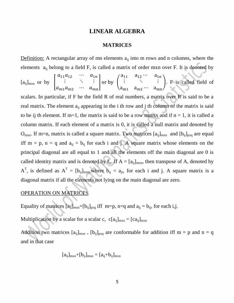
5
LINEAR ALGEBRA
MATRICES
Definition: A rectangular array of mn elements aij into m rows and n columns, where the
elements aij belong to a field F, is called a matrix of order mxn over F. It is denoted by
[aij]mxn or by [
] (
). F is called field of
scalars. In particular, if F be the field R of real numbers, a matrix over R is said to be a
real matrix. The element aij appearing in the i th row and j th column of the matrix is said
to be ij th element. If m=1, the matrix is said to be a row matrix and if n = 1, it is called a
column matrix. If each element of a matrix is 0, it is called a null matrix and denoted by
Omxn. If m=n, matrix is called a square matrix. Two matrices [aij]mxn and [bij]pxq are equal
iff m = p, n = q and aij = bij for each i and j. A square matrix whose elements on the
principal diagonal are all equal to 1 and all the elements off the main diagonal are 0 is
called identity matrix and is denoted by In. If A = [aij]mxn, then transpose of A, denoted by
AT, is defined as A
T = [bij]nxm,where bij = aji, for each i and j. A square matrix is a
diagonal matrix if all the elements not lying on the main diagonal are zero.
OPERATION ON MATRICES
Equality of matrices [aij]mxn=[bij]pxq iff m=p, n=q and aij = bij, for each i,j.
Multiplication by a scalar for a scalar c, c[aij]mxn = [caij]mxn
Addition two matrices [aij]mxn , [bij]pxq are conformable for addition iff m = p and n = q
and in that case
[aij]mxn+[bij]mxn = [aij+bij]mxn
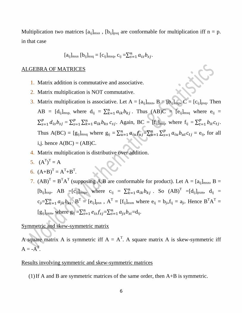
6
Multiplication two matrices [aij]mxn , [bij]pxq are conformable for multiplication iff n = p.
in that case
[aij]mxn [bij]nxq = [cij]mxq, cij =∑ .
ALGEBRA OF MATRICES
1. Matrix addition is commutative and associative.
2. Matrix multiplication is NOT commutative.
3. Matrix multiplication is associative. Let A = [aij]mxn, B = [bij]nxp, C = [cij]pxq. Then
AB = [dij]mxp, where dij = ∑ . Thus (AB)C = [eij]mxq where eij =
∑ = ∑ ∑
. Again, BC = [fij]nxq, where fij = ∑
.
Thus A(BC) = [gij]mxq where gij = ∑ =∑ ∑
= eij, for all
i,j. hence A(BC) = (AB)C.
4. Matrix multiplication is distributive over addition.
5. (AT)
T = A
6. (A+B)T = A
T+B
T.
7. (AB)T = B
TA
T (supposing A,B are conformable for product). Let A = [aij]mxn, B =
[bij]nxp. AB =[cij]mxp, where cij = ∑ . So (AB)
T =[dij]pxm, dij =
cji=∑ . B
T = [eij]pxn , A
T = [fij]nxm where eij = bji,fij = aji. Hence B
TA
T =
[gij]pxm, where gij =∑ =∑
=dij.
Symmetric and skew-symmetric matrix
A square matrix A is symmetric iff A = AT. A square matrix A is skew-symmetric iff
A = -AT.
Results involving symmetric and skew-symmetric matrices
(1) If A and B are symmetric matrices of the same order, then A+B is symmetric.
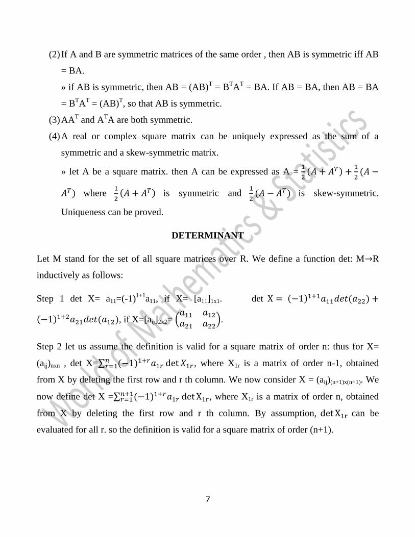
7
(2) If A and B are symmetric matrices of the same order , then AB is symmetric iff AB
= BA.
» if AB is symmetric, then AB = (AB)T = B
TA
T = BA. If AB = BA, then AB = BA
= BTA
T = (AB)
T, so that AB is symmetric.
(3) AAT and A
TA are both symmetric.
(4) A real or complex square matrix can be uniquely expressed as the sum of a
symmetric and a skew-symmetric matrix.
» let A be a square matrix. then A can be expressed as A =
(
(
where
( is symmetric and
( is skew-symmetric.
Uniqueness can be proved.
DETERMINANT
Let M stand for the set of all square matrices over R. We define a function det: M R
inductively as follows:
Step 1 det X= a11=(-1)1+1
a11, if X= [a11]1x1. det ( (
( ( , if X=[aij]2x2= (
).
Step 2 let us assume the definition is valid for a square matrix of order n: thus for X=
(aij)nxn , det X=∑ ( , where X1r is a matrix of order n-1, obtained
from X by deleting the first row and r th column. We now consider X = (aij)(n+1)x(n+1). We
now define det X =∑ ( , where X1r is a matrix of order n, obtained
from X by deleting the first row and r th column. By assumption, can be
evaluated for all r. so the definition is valid for a square matrix of order (n+1).
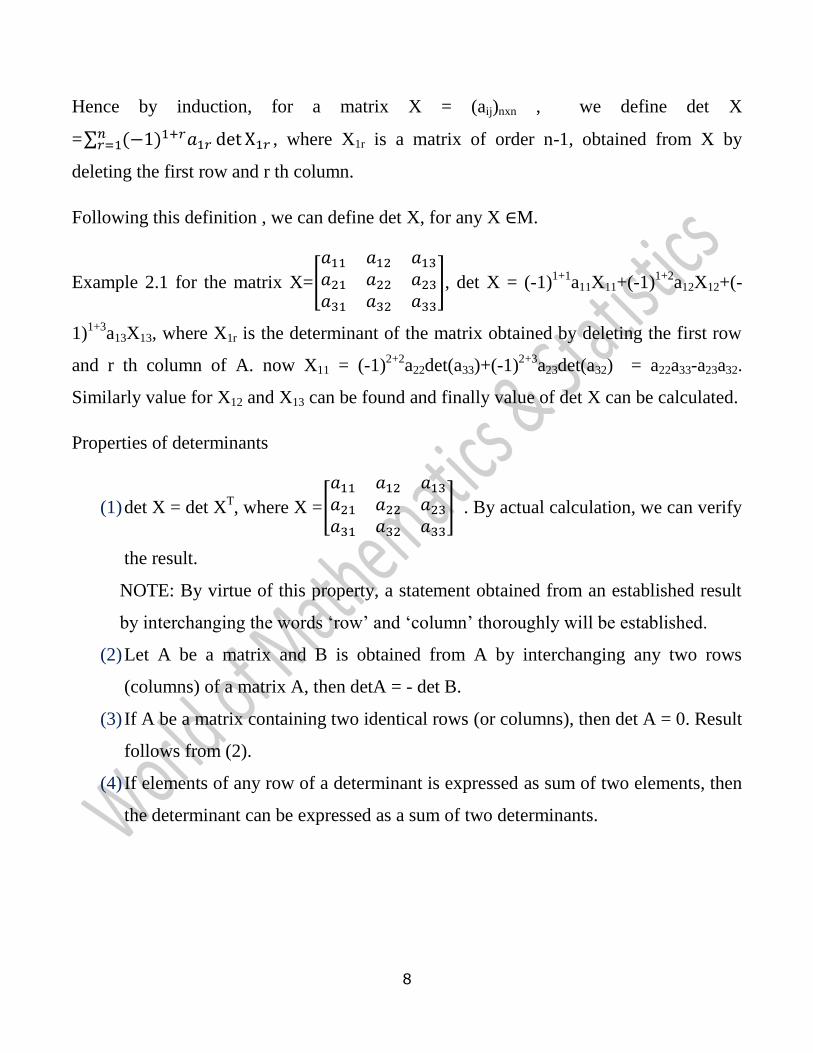
8
Hence by induction, for a matrix X = (aij)nxn , we define det X
=∑ ( , where X1r is a matrix of order n-1, obtained from X by
deleting the first row and r th column.
Following this definition , we can define det X, for any X M.
Example 2.1 for the matrix X=[
], det X = (-1)1+1
a11X11+(-1)1+2
a12X12+(-
1)1+3
a13X13, where X1r is the determinant of the matrix obtained by deleting the first row
and r th column of A. now X11 = (-1)2+2
a22det(a33)+(-1)2+3
a23det(a32) = a22a33-a23a32.
Similarly value for X12 and X13 can be found and finally value of det X can be calculated.
Properties of determinants
(1) det X = det XT, where X =[
] . By actual calculation, we can verify
the result.
NOTE: By virtue of this property, a statement obtained from an established result
by interchanging the words ‘row’ and ‘column’ thoroughly will be established.
(2) Let A be a matrix and B is obtained from A by interchanging any two rows
(columns) of a matrix A, then detA = - det B.
(3) If A be a matrix containing two identical rows (or columns), then det A = 0. Result
follows from (2).
(4) If elements of any row of a determinant is expressed as sum of two elements, then
the determinant can be expressed as a sum of two determinants.
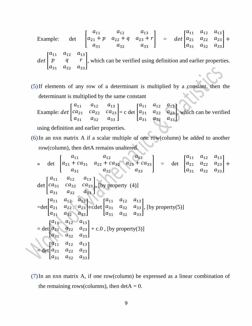
9
Example: det [
] = [
]
[
], which can be verified using definition and earlier properties.
(5) If elements of any row of a determinant is multiplied by a constant, then the
determinant is multiplied by the same constant
Example [
]= c det [
], which can be verified
using definition and earlier properties.
(6) In an nxn matrix A if a scalar multiple of one row(column) be added to another
row(column), then detA remains unaltered.
» det [
] = det [
]
[
], [by property (4)]
=det[
]+c [
], [by property(5)]
= det[
] + c.0 , [by property(3)]
= det[
]
(7) In an nxn matrix A, if one row(column) be expressed as a linear combination of
the remaining rows(columns), then detA = 0.
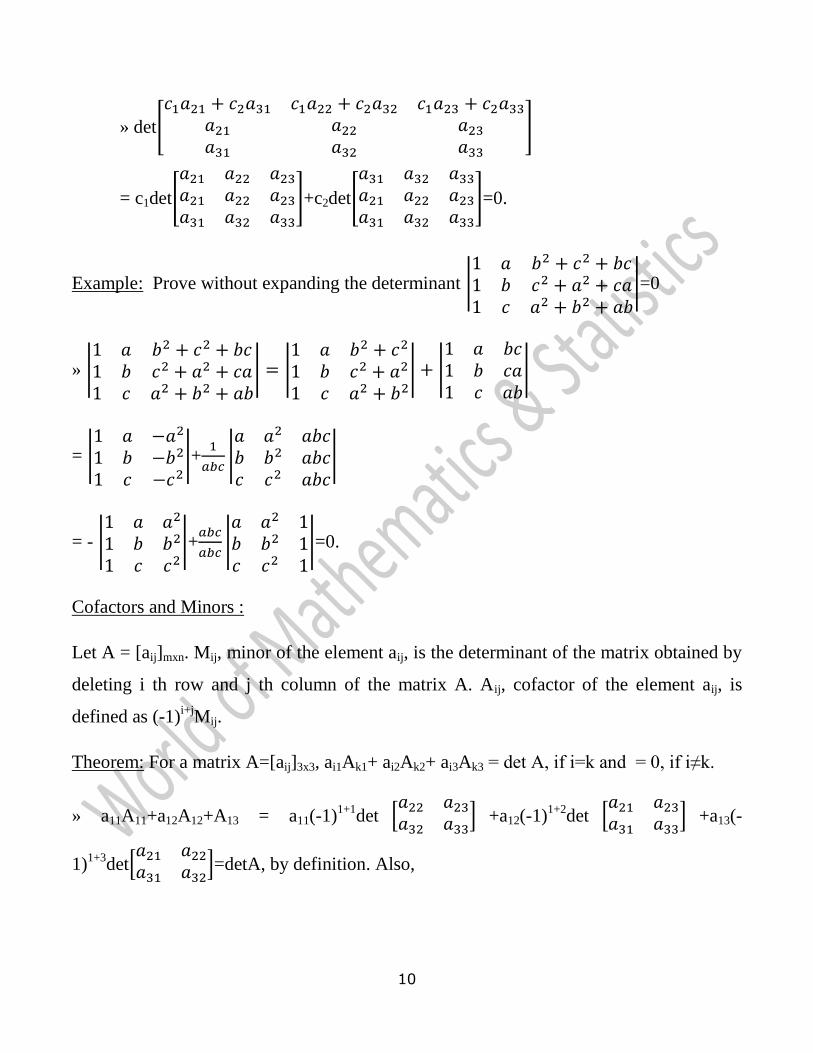
10
» det[
]
= c1det[
]+c2det[
]=0.
Example: Prove without expanding the determinant |
|=0
» |
| |
| |
|
= |
|+
|
|
= - |
|+
|
|=0.
Cofactors and Minors :
Let A = [aij]mxn. Mij, minor of the element aij, is the determinant of the matrix obtained by
deleting i th row and j th column of the matrix A. Aij, cofactor of the element aij, is
defined as (-1)i+j
Mij.
Theorem: For a matrix A=[aij]3x3, ai1Ak1+ ai2Ak2+ ai3Ak3 = det A, if i=k and = 0, if i≠k.
» a11A11+a12A12+A13 = a11(-1)1+1
det *
+ +a12(-1)
1+2det *
+ +a13(-
1)1+3
det*
+=detA, by definition. Also,
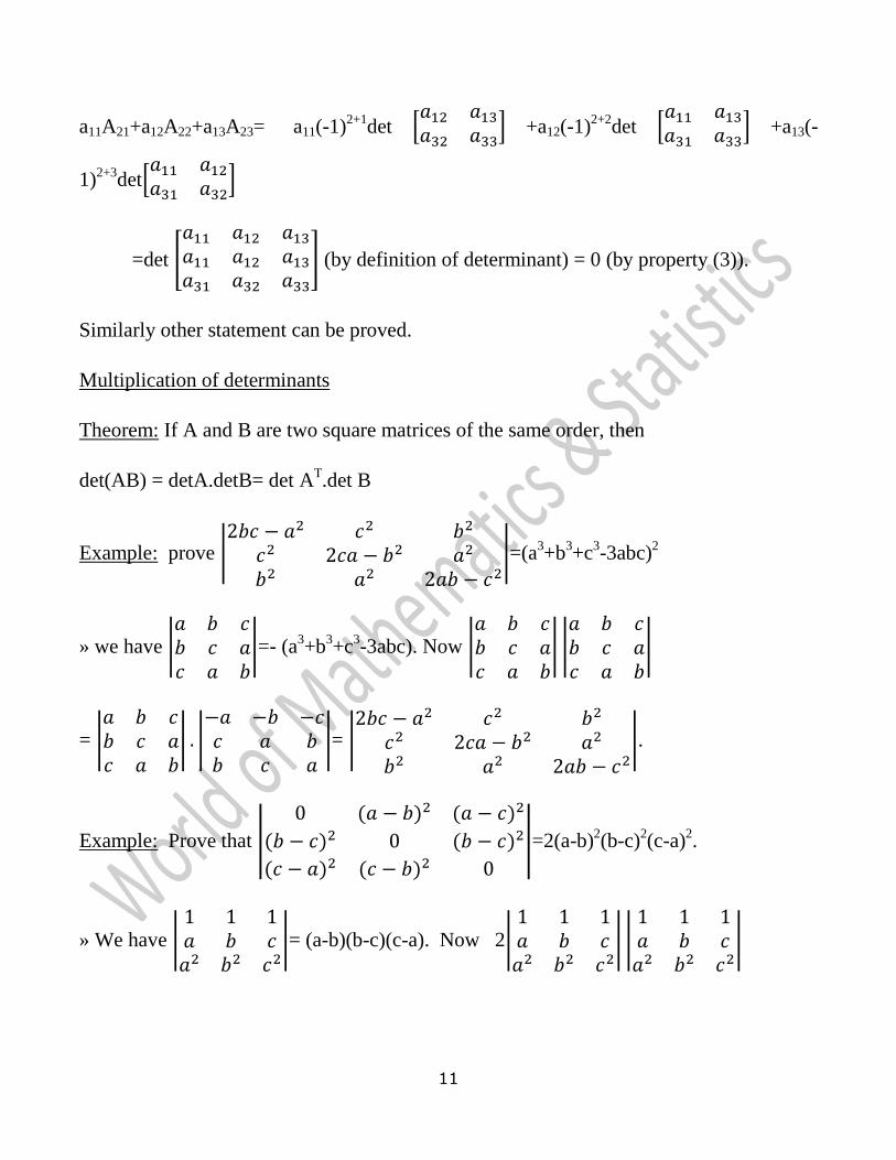
11
a11A21+a12A22+a13A23= a11(-1)2+1
det *
+ +a12(-1)
2+2det *
+ +a13(-
1)2+3
det*
+
=det [
] (by definition of determinant) = 0 (by property (3)).
Similarly other statement can be proved.
Multiplication of determinants
Theorem: If A and B are two square matrices of the same order, then
det(AB) = detA.detB= det AT.det B
Example: prove |
|=(a3+b
3+c
3-3abc)
2
» we have |
|=- (a3+b
3+c
3-3abc). Now |
| |
|
= |
| |
|= |
|.
Example: Prove that |
( (
( (
( (
|=2(a-b)2(b-c)
2(c-a)
2.
» We have |
|= (a-b)(b-c)(c-a). Now 2|
| |
|
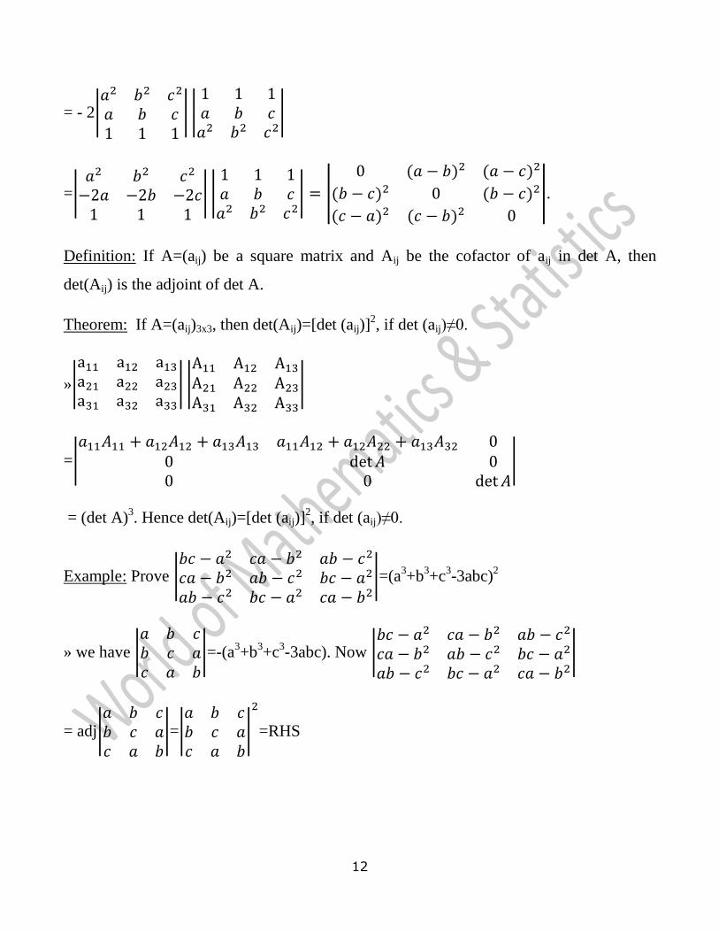
12
= - 2|
| |
|
=|
| |
| |
( (
( (
( (
|.
Definition: If A=(aij) be a square matrix and Aij be the cofactor of aij in det A, then
det(Aij) is the adjoint of det A.
Theorem: If A=(aij)3x3, then det(Aij)=[det (aij)]2, if det (aij)≠0.
»|
| |
|
=|
|
= (det A)3. Hence det(Aij)=[det (aij)]
2, if det (aij)≠0.
Example: Prove |
|=(a3+b
3+c
3-3abc)
2
» we have |
|=-(a3+b
3+c
3-3abc). Now |
|
= adj|
|=|
|
=RHS
13
Adjoint of a square matrix
Definition Let A = (aij) be a square matrix. Let Aij be the cofactor of aij in detA. The
adjoint of A, denoted by Adj A, is defined as (Aij)T.
Theorem: Let A be a square matrix of order n. then A. (Adj A) = (Adj A).A = | |In.
» the i,j th element of A.(Adj A) is ai1A1j+ai2AI2+…+ainAnj which equals 0, if i≠j and
equals | |, if i=j. Hence A. (Adj A) = [| |
| |
] = | |In. similarly other part.
Definition: A square matrix is singular if | |=0 and is non-singular if | |≠0.
Definition: A square matrix of order n is invertible if there exists a matrix B such that
AB= BA = In. B is called an inverse to A. If C be an inverse to A also, then AC = CA =
In. using associativity of product of matrices, it is easy to verify that B = C. So inverse of
a square matrix , if it exists, is unique. Note also that since AB and BA both are to be
defined, A must be a square matrix.
Theorem: An nxn matrix A is invertible iff it is non-singular.
» Necessity let Anxn be invertible. Then there exists Bnxn such that AB = BA = In. then
| || |=| |=| |=1 so that | |≠0.
Sufficiency Let | | ≠0. we know that A.(Adj A) = (Adj A).A = | | In. hence
A.
| |( =
| |( A = In, proving the result.
14
Theorem: If A,B be invertible matrices of the same order, then AB is invertible and
(AB)-1
= B-1
A-1
.
» | | | || |≠0, hence AB is invertible. Using associativity,
(AB)(B-1
A-1
) = In=(B-1
A-1
)(AB).
Theorem: If A be invertible, then A-1
is also invertible and (A-1
)-1
= A.
» From AA-1
= A-1
A = In, it follows from the definition of inverse that (A-1
)-1
= A.
Theorem: If A be an invertible matrix, then AT is invertible and (A
T)
-1 = (A
-1)
T.
» AT.(A
-1)
T = (A
-1A)
T=In
T = In = (AA
-1)
T = (A
-1)
T.A
T. Hence (A
T)
-1 = (A
-1)
T.
Orthogonal matrix
Definition: A square matrix A of order n is orthogonal iff AAT = In.
Theorem: If A is orthogonal , then A is non-singular and | |=±1.
» | | | || | | | | | implies | | .
Theorem: If A be an nxn orthogonal matrix, then ATA = In.
» AAT = In⇒A
T(AA
T) = A
TIn⇒(A
TA)A
T = A
T⇒(ATA-In)A
T = O⇒(A
TA-In)[A
T(A
T)
-1] = O
(A is orthogonal⇒A is non-singular⇒AT is non-singular⇒A
T is invertible) ⇒A
TA = In.
Theorem: If A and B are orthogonal matrices of the same order, then AB is orthogonal.
»(AB)(AB)T = (AB)(B
TA
T) = A(BB
T)A
T =(AIn)A
T = AA
T = In.
Theorem: If A is orthogonal, A-1
is orthogonal.
» (A-1
)(A-1
)T=(A
-1)(A
T)
-1= (A
TA)
-1 = In
-1 = In.
Note: If A be an orthogonal matrix, AT = A
-1.
15
Rank of a matrix
Definition Let A be a non-zero matrix of order mxn. Rank of A is defined to be the
greatest positive integer r such that the determinant of the matrix formed by elements of
A lying at the intersection of some r rows and some r columns is nonzero. Rank of null
matrix is defined to be zero.
Note: (1) 0<rank A≤ min{m,n}, for a non-zero matrix A.
(2) for a square matrix A of order n, rankA < n or =n according as A is singular or
non-singular.
(3) Rank A = Rank AT.
Elementary row operations
An elementary operation on a matrix A over a field F is an operation of the following
three types:
Interchange of two rows(columns) of A
Multiplication of a row (or column) by a non-zero scalar c F
Addition of a scalar multiple of one row (or column)to another row(or column)
When applied to rows, elementary operations are called elementary row operations.
Notation: interchange of i th and j th row will be denoted by Rij. Multiplication of i th row
by c will be denoted by cRi. Addition of c times the j th row to the i th row is denoted by
Ri+cRj.
Definition: An mxn matrix B is row equivalent to a mxn matrix A over the same field F
iff B can be obtained from A by a finite number of successive elementary row operations.
16
Note Since inverse of an elementary row operation is again an elementary row operation,
if B is row equivalent to A, then A is also row equivalent to B.
Definition: An m x n matrix is row reduced iff
The first non-zero element in a non-zero row is 1 and
each column containing the leading 1of some row has all other elements zero.
Example: [
]
Definition: An m x n matrix A is row reduced echelon matrix iff
A is row reduced
Each zero row comes below each non-zero row and
If first r rows are non-zero rows of A and if the leading element of row I occurs in
column ki, then k1<k2<…<kr.
Example: [
]
Algorithm which row-reduces a matrix to echelon form
Step-1: suppose that j1 column is the first column with a nonzero entry. Interchange the
rows so that this nonzero entry appears in the first row, that is, so that ≠0
Step-2: for each i>1, apply the operation Ri→- .
Repeat steps 1 and 2 with the submatrix formed by all the rows excluding the first.
Theorem: For a given matrix A , a row-reduced echelon matrix B equivalent to A can be
found by elementary row operations.

17
Example: [
]
→ [
]
→ [
]
→ [
]
→ [
]
→ [
]
Theorem: If a matrix A is equivalent to a row-reduced enhelon matrix having r non-zero
rows, then Rank A = r.
Example: Find the rank of the matrix A = [
]
» First Method: rank A≥ 1, since = 1≠0. Though det*
+ = 0, det*
+≠0.
Hence rank A≥ 2. Since det A= 0, rank A is not equal to 3. hence rank A = 2.
Second Method: A
→ [
]
→ [
]
→ [
]
→ [
]. Hence rank A = 2.
SYSTEM OF LINEAR EQUATIONS
A system of m linear equation in n unknowns x1,x2,…,xn is of the form
a11x1+a12x2+…+a1nxn = b1
a21x1+a22x2+…+a2nxn = b2
…….................................
am1x1+am2x2+…+amnxn = bm, where aij’s and bi’s are given elements of a field.
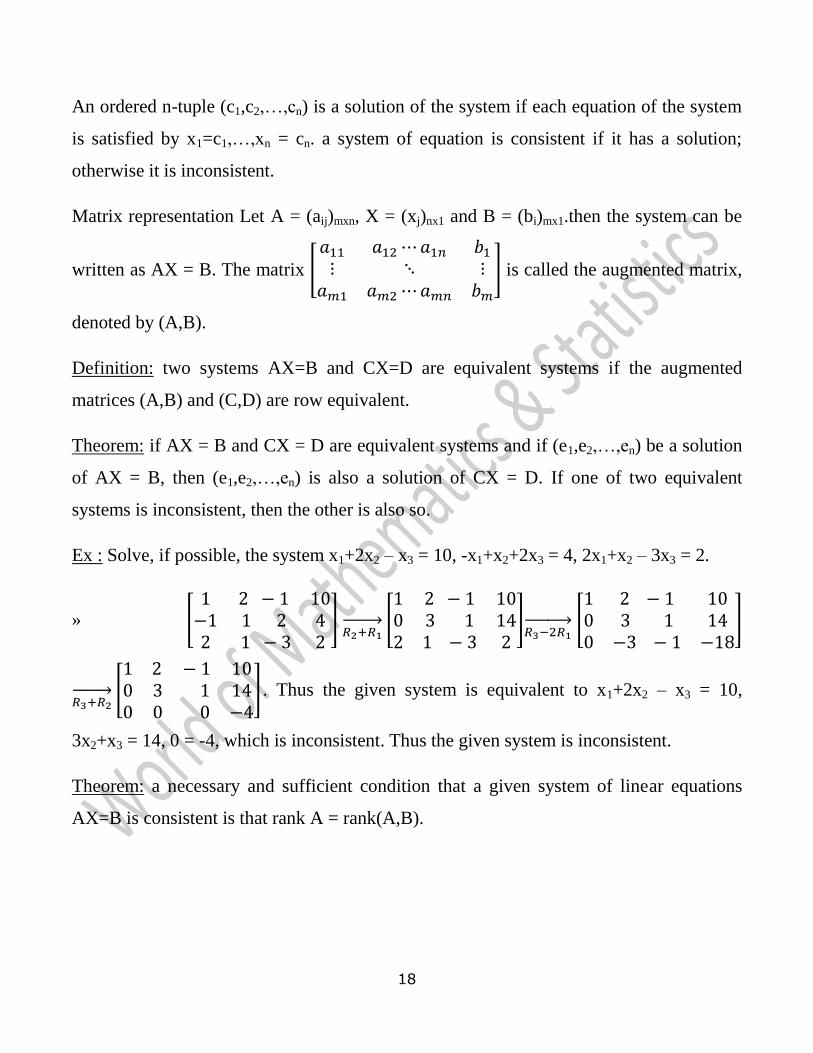
18
An ordered n-tuple (c1,c2,…,cn) is a solution of the system if each equation of the system
is satisfied by x1=c1,…,xn = cn. a system of equation is consistent if it has a solution;
otherwise it is inconsistent.
Matrix representation Let A = (aij)mxn, X = (xj)nx1 and B = (bi)mx1.then the system can be
written as AX = B. The matrix [
] is called the augmented matrix,
denoted by (A,B).
Definition: two systems AX=B and CX=D are equivalent systems if the augmented
matrices (A,B) and (C,D) are row equivalent.
Theorem: if AX = B and CX = D are equivalent systems and if (e1,e2,…,en) be a solution
of AX = B, then (e1,e2,…,en) is also a solution of CX = D. If one of two equivalent
systems is inconsistent, then the other is also so.
Ex : Solve, if possible, the system x1+2x2 – x3 = 10, -x1+x2+2x3 = 4, 2x1+x2 – 3x3 = 2.
» [
]
→ [
]
→ [
]
→ [
] . Thus the given system is equivalent to x1+2x2 – x3 = 10,
3x2+x3 = 14, 0 = -4, which is inconsistent. Thus the given system is inconsistent.
Theorem: a necessary and sufficient condition that a given system of linear equations
AX=B is consistent is that rank A = rank(A,B).
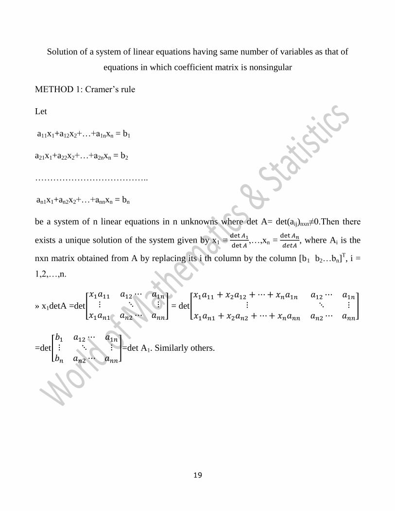
19
Solution of a system of linear equations having same number of variables as that of
equations in which coefficient matrix is nonsingular
METHOD 1: Cramer’s rule
Let
a11x1+a12x2+…+a1nxn = b1
a21x1+a22x2+…+a2nxn = b2
………………………………..
an1x1+an2x2+…+annxn = bn
be a system of n linear equations in n unknowns where det A= det(aij)nxn≠0.Then there
exists a unique solution of the system given by x1 =
,…,xn =
, where Ai is the
nxn matrix obtained from A by replacing its i th column by the column [b1 b2…bn]T, i =
1,2,…,n.
» x1detA =det[
] = det[
]
=det[
]=det A1. Similarly others.
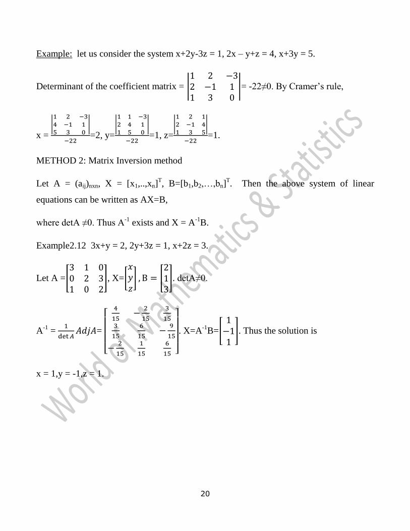
20
Example: let us consider the system x+2y-3z = 1, 2x – y+z = 4, x+3y = 5.
Determinant of the coefficient matrix = |
|= -22≠0. By Cramer’s rule,
x =
|
|
=2, y=
|
|
=1, z=
|
|
=1.
METHOD 2: Matrix Inversion method
Let A = (aij)nxn, X = [x1,..,xn]T, B=[b1,b2,…,bn]
T. Then the above system of linear
equations can be written as AX=B,
where detA ≠0. Thus A-1
exists and X = A-1
B.
Example2.12 3x+y = 2, 2y+3z = 1, x+2z = 3.
Let A =[
], X=[ ] [
]. detA≠0.
A-1
=
=
[
]
. X=A-1
B=[
]. Thus the solution is
x = 1,y = -1,z = 1.
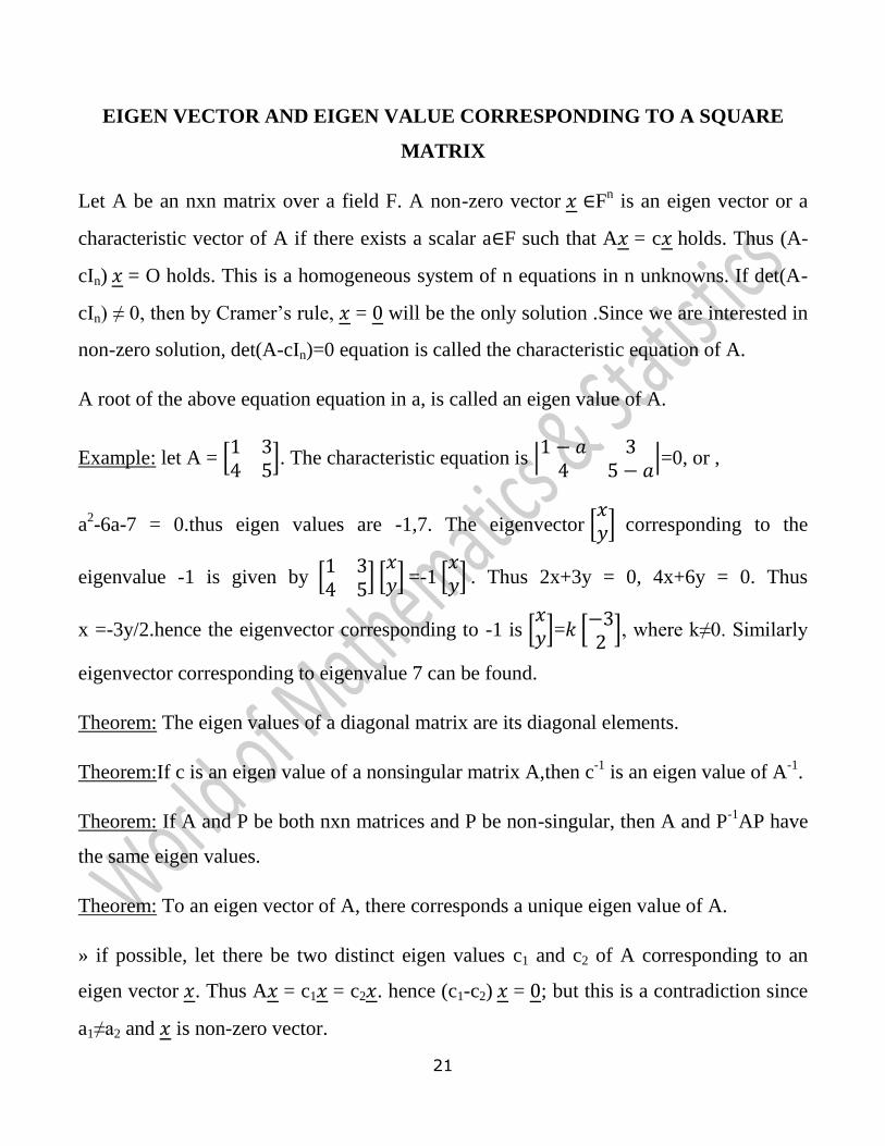
21
EIGEN VECTOR AND EIGEN VALUE CORRESPONDING TO A SQUARE
MATRIX
Let A be an nxn matrix over a field F. A non-zero vector Fn is an eigen vector or a
characteristic vector of A if there exists a scalar a F such that A = c holds. Thus (A-
cIn) = O holds. This is a homogeneous system of n equations in n unknowns. If det(A-
cIn) ≠ 0, then by Cramer’s rule, = will be the only solution .Since we are interested in
non-zero solution, det(A-cIn)=0 equation is called the characteristic equation of A.
A root of the above equation equation in a, is called an eigen value of A.
Example: let A = *
+. The characteristic equation is |
|=0, or ,
a2-6a-7 = 0.thus eigen values are -1,7. The eigenvector *
+ corresponding to the
eigenvalue -1 is given by *
+ * + =-1 *
+ . Thus 2x+3y = 0, 4x+6y = 0. Thus
x =-3y/2.hence the eigenvector corresponding to -1 is * += *
+, where k≠0. Similarly
eigenvector corresponding to eigenvalue 7 can be found.
Theorem: The eigen values of a diagonal matrix are its diagonal elements.
Theorem:If c is an eigen value of a nonsingular matrix A,then c-1
is an eigen value of A-1
.
Theorem: If A and P be both nxn matrices and P be non-singular, then A and P-1
AP have
the same eigen values.
Theorem: To an eigen vector of A, there corresponds a unique eigen value of A.
» if possible, let there be two distinct eigen values c1 and c2 of A corresponding to an
eigen vector . Thus A = c1 = c2 . hence (c1-c2) = ; but this is a contradiction since
a1≠a2 and is non-zero vector.
22
Theorem: (Cayley Hamilton theorem)
Every square matrix satisfies its own characteristic equation.
Ex: let A=*
+. Verify that A satisfies its characteristic equation. Hence find A-1
.
» The characteristic equation is x2 – 7x+7 = 0. Now A
2-7A+7I =O can be verified by
actual calculation. Hence Cayley Hamilton theorem is verified. Hence A *
(
+=I2. Thus A-1
=
( =
*
+.
REAL QUADRATIC FORM
An expression of the form ∑ (i,j = 1,2,…,n) where aijare real and aij = aji, is said
to be a real quadratic form in n variables x1,x2,…,xn. the matrix notation for the quadratic
form is TA , where = T
, A = (aij)nxn. A is a real symmetric matrix
since aij = aji for all i,j. A is called the matrix associated with the quadratic form.
Example2.27 x1x2-x2x3 is a real quadratic form in three variables x1,x2,x3. The associated
matrix is [
].
23
Definition: A real quadratic form Q= TA is
(1) Positive definite if Q>0 for all ≠O
(2) Positive semi definiteif Q≥0 for all ≠O
(3) Negative definite if Q<0 for all ≠O
(4) Negative semidefinite if Q≤0 for all ≠O
(5) Indefinite if Q≥0 for some ≠O and Q≤0 for some other ≠O
Example: consider the quadratic form Q(x1,x2,x3) = x12+2x2
2+4x3
2+2x1x2-4x2x3-2x3x1 =
(x1+x2-x3)2+(x2-x3)
2+2x3
2≥0 and Q = 0 only when x1+x2-x3= x2-x3 = x3 = 0, that is, when
x1=x2=x3 = 0. Thus Q is positive definite.
For a real quadratic form Q=XTAX where A is real symmetric matrix of rank r(≤n), there
exists a non-singular matrix P such that PTAP becomes a diagonal matrix
[
] of rank r, where 0≤m≤r. thus by a suitable transformation X=PY,
where P is nonsingular, the real quadratic form Q transforms to y12+…+ym
2-ym+1
2-…-yr
2
where 0≤m≤r≤n. this is called normal form of Q.
Theorem: A real quadratic form of rank r and index m is
(1) Positive definite, if r = n,m=r
(2) Positive semidefinite, if r<n,m= r
(3) Negative definite, if r = n,m = 0
(4) Negative semidefinite, if r<n,m= 0
(5) Indefinite, if r≤n,0<m<r
24
Example: Reduce the quadratic form 5x2+y
2+14z
2-4yz-10zx to its normal form and show
that it is positive definite.
» The associated symmetric matrix is A= [
] . Let us apply congruent
operations on A to reduce it to the normal form.
A → [
] → [
] → [
] → [
]
√
√
→ [√
√
]
√
√
→ [
]. The normal form is x2+y
2+z
2.the rank of the
quadratic form is 3 and its signature is 3. Thus the quadratic form is positive definite.
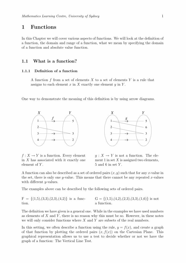
X Y
1
2
3
4
5
3
2
f
X Y
1
2
3
4
5
3
6
2
g
Mathematics Learning Centre, University of Sydney 1
1 Functions
In this Chapter we will cover various aspects of functions. We will look at the definition ofa function, the domain and range of a function, what we mean by specifying the domainof a function and absolute value function.
1.1 What is a function?
1.1.1 Definition of a function
A function f from a set of elements X to a set of elements Y is a rule thatassigns to each element x in X exactly one element y in Y .
One way to demonstrate the meaning of this definition is by using arrow diagrams.
f : X → Y is a function. Every elementin X has associated with it exactly oneelement of Y .
g : X → Y is not a function. The ele-ment 1 in set X is assigned two elements,5 and 6 in set Y .
A function can also be described as a set of ordered pairs (x, y) such that for any x-value inthe set, there is only one y-value. This means that there cannot be any repeated x-valueswith different y-values.
The examples above can be described by the following sets of ordered pairs.
F = {(1,5),(3,3),(2,3),(4,2)} is a func-tion.
G = {(1,5),(4,2),(2,3),(3,3),(1,6)} is nota function.
The definition we have given is a general one. While in the examples we have used numbersas elements of X and Y , there is no reason why this must be so. However, in these noteswe will only consider functions where X and Y are subsets of the real numbers.
In this setting, we often describe a function using the rule, y = f(x), and create a graphof that function by plotting the ordered pairs (x, f(x)) on the Cartesian Plane. Thisgraphical representation allows us to use a test to decide whether or not we have thegraph of a function: The Vertical Line Test.
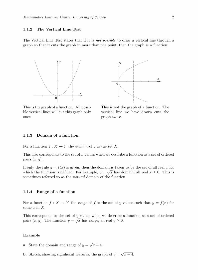
0
x
y
y
0
x
Mathematics Learning Centre, University of Sydney 2
1.1.2 The Vertical Line Test
The Vertical Line Test states that if it is not possible to draw a vertical line through agraph so that it cuts the graph in more than one point, then the graph is a function.
This is the graph of a function. All possi-ble vertical lines will cut this graph onlyonce.
This is not the graph of a function. Thevertical line we have drawn cuts thegraph twice.
1.1.3 Domain of a function
For a function f : X → Y the domain of f is the set X.
This also corresponds to the set of x-values when we describe a function as a set of orderedpairs (x, y).
If only the rule y = f(x) is given, then the domain is taken to be the set of all real x forwhich the function is defined. For example, y =
√x has domain; all real x ≥ 0. This is
sometimes referred to as the natural domain of the function.
1.1.4 Range of a function
For a function f : X → Y the range of f is the set of y-values such that y = f(x) forsome x in X.
This corresponds to the set of y-values when we describe a function as a set of orderedpairs (x, y). The function y =
√x has range; all real y ≥ 0.
Example
a. State the domain and range of y =√
x + 4.
b. Sketch, showing significant features, the graph of y =√
x + 4.
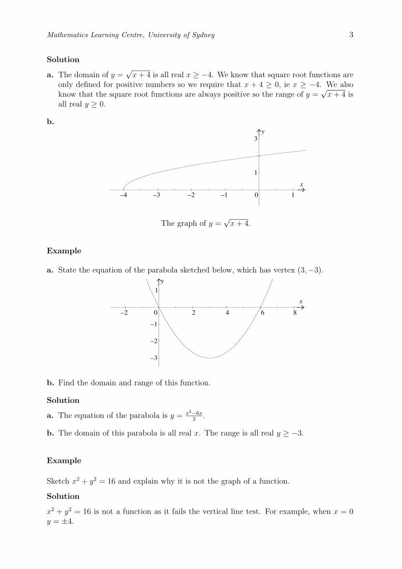
–4 –2 –1
x
y
10
1
–3
3
1
–2
x
y
0 2 4 6 8
–1
–2
–3
Mathematics Learning Centre, University of Sydney 3
Solution
a. The domain of y =√
x + 4 is all real x ≥ −4. We know that square root functions areonly defined for positive numbers so we require that x + 4 ≥ 0, ie x ≥ −4. We alsoknow that the square root functions are always positive so the range of y =
√x + 4 is
all real y ≥ 0.
b.
The graph of y =√
x + 4.
Example
a. State the equation of the parabola sketched below, which has vertex (3,−3).
b. Find the domain and range of this function.
Solution
a. The equation of the parabola is y = x2−6x3
.
b. The domain of this parabola is all real x. The range is all real y ≥ −3.
Example
Sketch x2 + y2 = 16 and explain why it is not the graph of a function.
Solution
x2 + y2 = 16 is not a function as it fails the vertical line test. For example, when x = 0y = ±4.
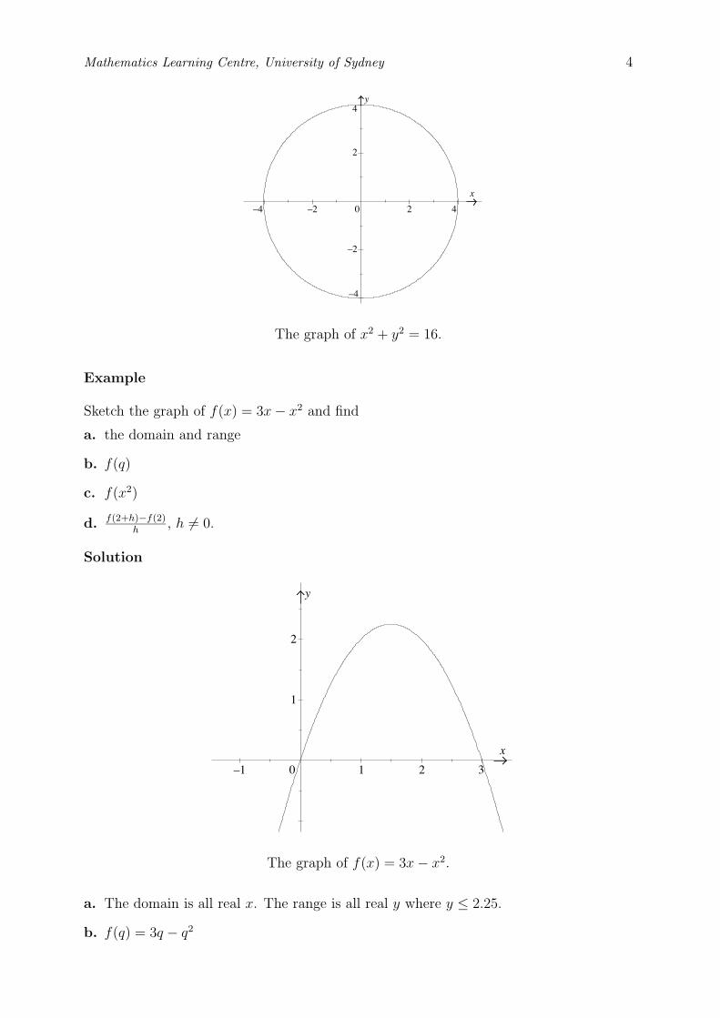
2
4
–4
y
0
–2
2 4–2
x
–4
0 21 3–1
1
2
x
y
Mathematics Learning Centre, University of Sydney 4
The graph of x2 + y2 = 16.
Example
Sketch the graph of f(x) = 3x − x2 and find
a. the domain and range
b. f(q)
c. f(x2)
d. f(2+h)−f(2)h
, h �= 0.
Solution
The graph of f(x) = 3x − x2.
a. The domain is all real x. The range is all real y where y ≤ 2.25.
b. f(q) = 3q − q2
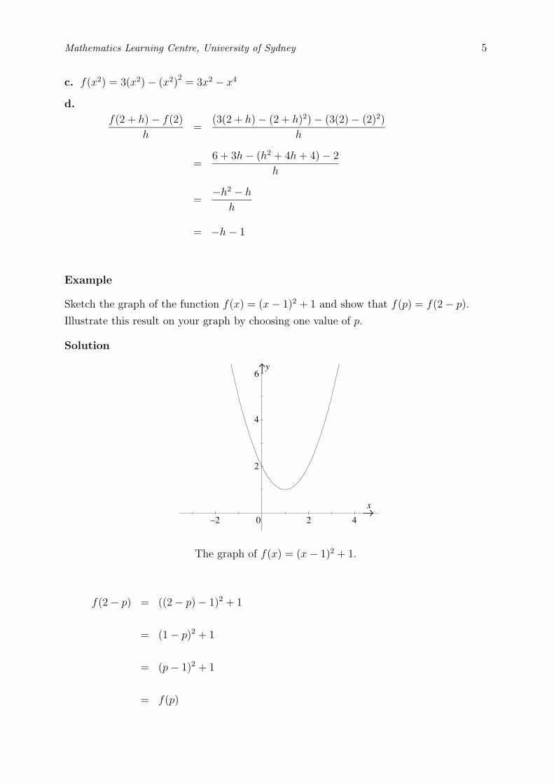
–2
x
2
4
6y
0 2 4
Mathematics Learning Centre, University of Sydney 5
c. f(x2) = 3(x2) − (x2)2
= 3x2 − x4
d.
f(2 + h) − f(2)
h=
(3(2 + h) − (2 + h)2) − (3(2) − (2)2)
h
=6 + 3h − (h2 + 4h + 4) − 2
h
=−h2 − h
h
= −h − 1
Example
Sketch the graph of the function f(x) = (x − 1)2 + 1 and show that f(p) = f(2 − p).
Illustrate this result on your graph by choosing one value of p.
Solution
The graph of f(x) = (x − 1)2 + 1.
f(2 − p) = ((2 − p) − 1)2 + 1
= (1 − p)2 + 1
= (p − 1)2 + 1
= f(p)
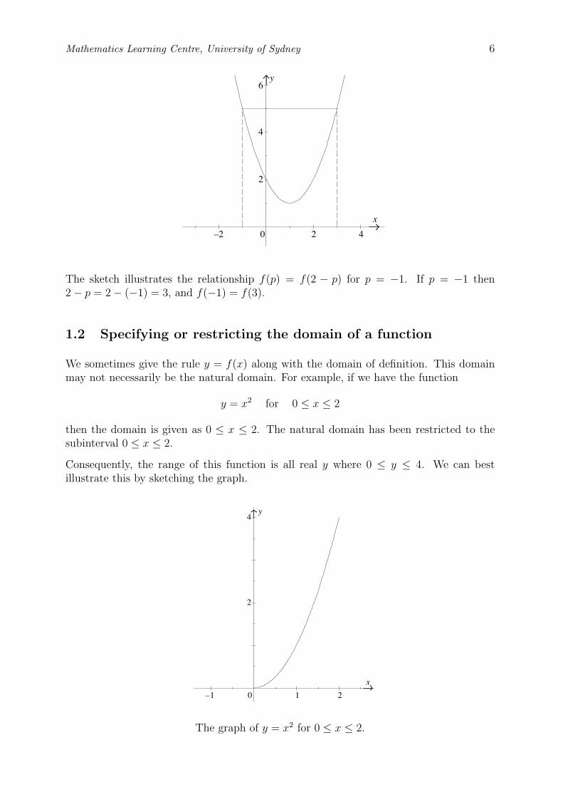
–2
x
2
4
6y
0 2 4
–1
x
2
4y
0 21
Mathematics Learning Centre, University of Sydney 6
The sketch illustrates the relationship f(p) = f(2 − p) for p = −1. If p = −1 then2 − p = 2 − (−1) = 3, and f(−1) = f(3).
1.2 Specifying or restricting the domain of a function
We sometimes give the rule y = f(x) along with the domain of definition. This domainmay not necessarily be the natural domain. For example, if we have the function
y = x2 for 0 ≤ x ≤ 2
then the domain is given as 0 ≤ x ≤ 2. The natural domain has been restricted to thesubinterval 0 ≤ x ≤ 2.
Consequently, the range of this function is all real y where 0 ≤ y ≤ 4. We can bestillustrate this by sketching the graph.
The graph of y = x2 for 0 ≤ x ≤ 2.
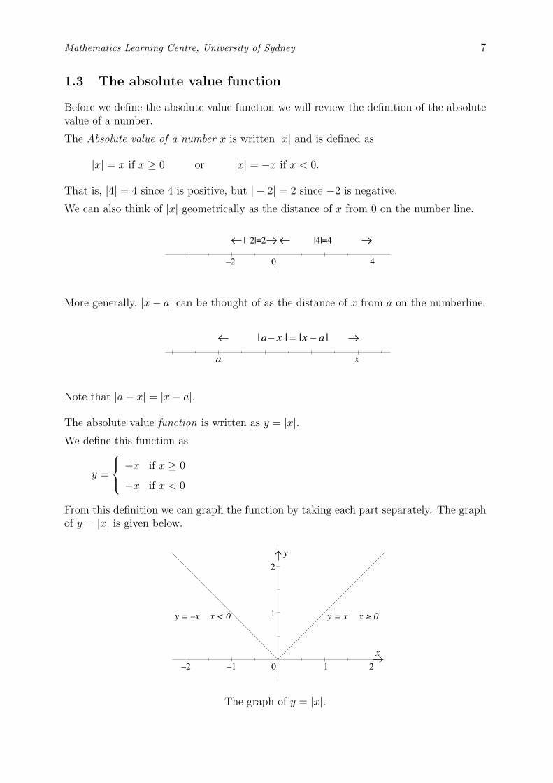
0 4–2
|–2|=2 |4|=4
a x
| | = | |a – x x – a
y = –x x < 0
y
1
1
2
0–1
x
2–2
y = x x ≥ 0
Mathematics Learning Centre, University of Sydney 7
1.3 The absolute value function
Before we define the absolute value function we will review the definition of the absolutevalue of a number.
The Absolute value of a number x is written |x| and is defined as
|x| = x if x ≥ 0 or |x| = −x if x < 0.
That is, |4| = 4 since 4 is positive, but | − 2| = 2 since −2 is negative.
We can also think of |x| geometrically as the distance of x from 0 on the number line.
More generally, |x − a| can be thought of as the distance of x from a on the numberline.
Note that |a − x| = |x − a|.
The absolute value function is written as y = |x|.We define this function as
y =
+x if x ≥ 0
−x if x < 0
From this definition we can graph the function by taking each part separately. The graphof y = |x| is given below.
The graph of y = |x|.
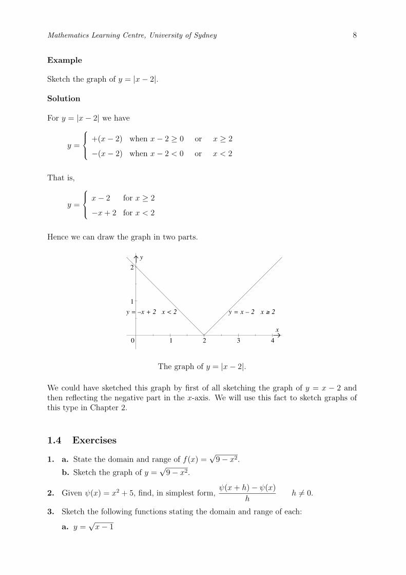
y
1
1
2
0
x
2
y = x – 2 x ≥ 2 y = –x + 2 x < 2
3 4
Mathematics Learning Centre, University of Sydney 8
Example
Sketch the graph of y = |x − 2|.
Solution
For y = |x − 2| we have
y =
+(x − 2) when x − 2 ≥ 0 or x ≥ 2
−(x − 2) when x − 2 < 0 or x < 2
That is,
y =
x − 2 for x ≥ 2
−x + 2 for x < 2
Hence we can draw the graph in two parts.
The graph of y = |x − 2|.
We could have sketched this graph by first of all sketching the graph of y = x − 2 andthen reflecting the negative part in the x-axis. We will use this fact to sketch graphs ofthis type in Chapter 2.
1.4 Exercises
1. a. State the domain and range of f(x) =√
9 − x2.
b. Sketch the graph of y =√
9 − x2.
2. Given ψ(x) = x2 + 5, find, in simplest form,ψ(x + h) − ψ(x)
hh �= 0.
3. Sketch the following functions stating the domain and range of each:
a. y =√
x − 1
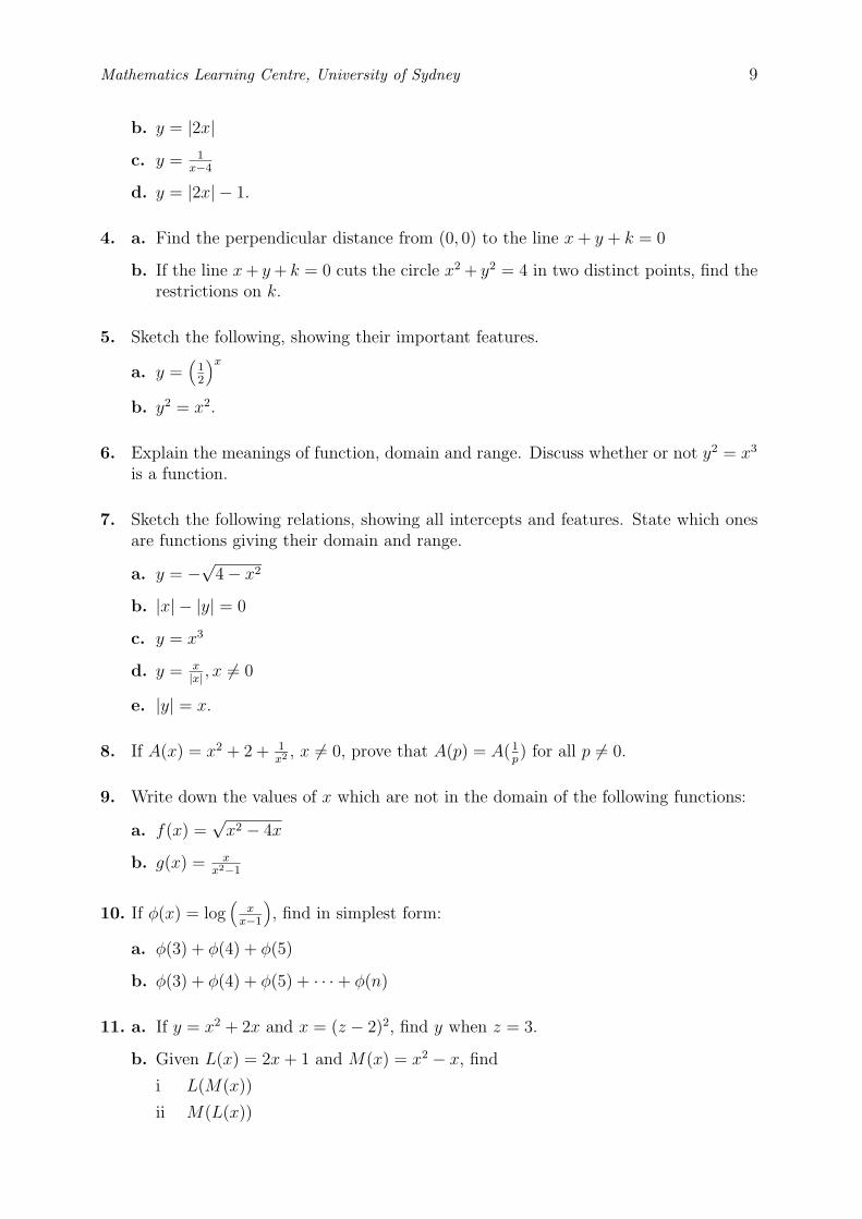
Mathematics Learning Centre, University of Sydney 9
b. y = |2x|c. y = 1
x−4
d. y = |2x| − 1.
4. a. Find the perpendicular distance from (0, 0) to the line x + y + k = 0
b. If the line x + y + k = 0 cuts the circle x2 + y2 = 4 in two distinct points, find therestrictions on k.
5. Sketch the following, showing their important features.
a. y =(
12
)x
b. y2 = x2.
6. Explain the meanings of function, domain and range. Discuss whether or not y2 = x3
is a function.
7. Sketch the following relations, showing all intercepts and features. State which onesare functions giving their domain and range.
a. y = −√
4 − x2
b. |x| − |y| = 0
c. y = x3
d. y = x|x| , x �= 0
e. |y| = x.
8. If A(x) = x2 + 2 + 1x2 , x �= 0, prove that A(p) = A(1
p) for all p �= 0.
9. Write down the values of x which are not in the domain of the following functions:
a. f(x) =√
x2 − 4x
b. g(x) = xx2−1
10. If φ(x) = log(
xx−1
), find in simplest form:
a. φ(3) + φ(4) + φ(5)
b. φ(3) + φ(4) + φ(5) + · · · + φ(n)
11. a. If y = x2 + 2x and x = (z − 2)2, find y when z = 3.
b. Given L(x) = 2x + 1 and M(x) = x2 − x, find
i L(M(x))
ii M(L(x))
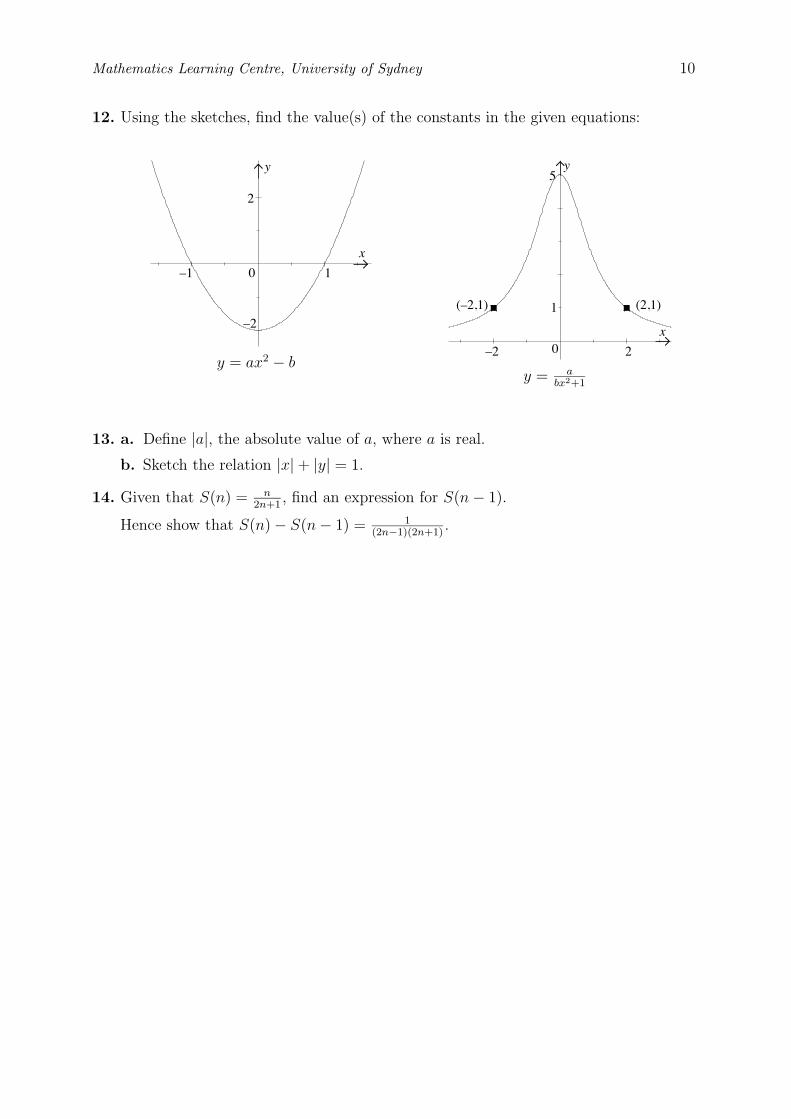
–1 1
x
y
2
0
–2
(–2,1)
0x
–2
y
2
1
5
(2,1)
Mathematics Learning Centre, University of Sydney 10
12. Using the sketches, find the value(s) of the constants in the given equations:
y = ax2 − by = a
bx2+1
13. a. Define |a|, the absolute value of a, where a is real.
b. Sketch the relation |x| + |y| = 1.
14. Given that S(n) = n2n+1
, find an expression for S(n − 1).
Hence show that S(n) − S(n − 1) = 1(2n−1)(2n+1)
.
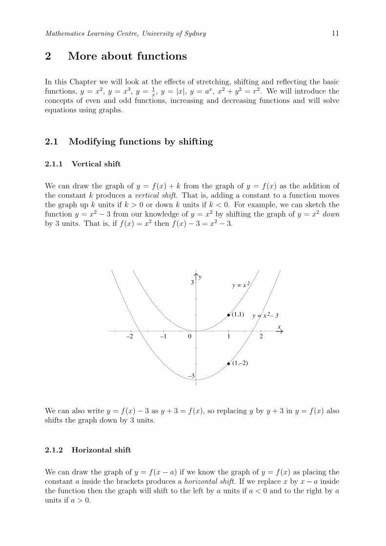
2
y
1–1–2 0
3
–3
2
(1,–2)
x
(1,1)
y = x 2
y = x – 3
Mathematics Learning Centre, University of Sydney 11
2 More about functions
In this Chapter we will look at the effects of stretching, shifting and reflecting the basicfunctions, y = x2, y = x3, y = 1
x, y = |x|, y = ax, x2 + y2 = r2. We will introduce the
concepts of even and odd functions, increasing and decreasing functions and will solveequations using graphs.
2.1 Modifying functions by shifting
2.1.1 Vertical shift
We can draw the graph of y = f(x) + k from the graph of y = f(x) as the addition ofthe constant k produces a vertical shift. That is, adding a constant to a function movesthe graph up k units if k > 0 or down k units if k < 0. For example, we can sketch thefunction y = x2 − 3 from our knowledge of y = x2 by shifting the graph of y = x2 downby 3 units. That is, if f(x) = x2 then f(x) − 3 = x2 − 3.
We can also write y = f(x) − 3 as y + 3 = f(x), so replacing y by y + 3 in y = f(x) alsoshifts the graph down by 3 units.
2.1.2 Horizontal shift
We can draw the graph of y = f(x − a) if we know the graph of y = f(x) as placing theconstant a inside the brackets produces a horizontal shift. If we replace x by x− a insidethe function then the graph will shift to the left by a units if a < 0 and to the right by aunits if a > 0.
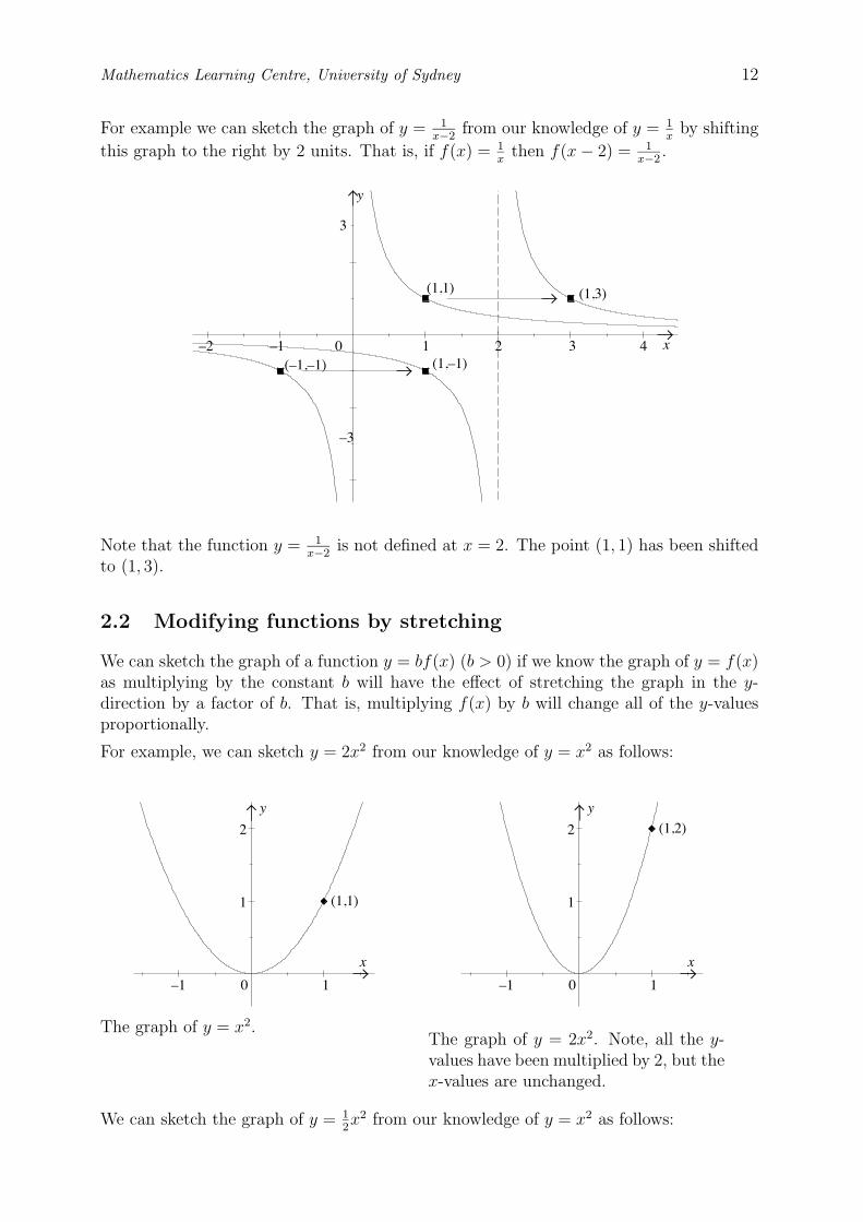
(–1,–1) (1,–1)
(1,1)
1–1–2
–3
0
3
2 x3 4
(1,3)
y
y
1
1
2
0–1
x
(1,1)
y
1
1
2
0–1
x
(1,2)
Mathematics Learning Centre, University of Sydney 12
For example we can sketch the graph of y = 1x−2
from our knowledge of y = 1x
by shifting
this graph to the right by 2 units. That is, if f(x) = 1x
then f(x − 2) = 1x−2
.
Note that the function y = 1x−2
is not defined at x = 2. The point (1, 1) has been shiftedto (1, 3).
2.2 Modifying functions by stretching
We can sketch the graph of a function y = bf(x) (b > 0) if we know the graph of y = f(x)as multiplying by the constant b will have the effect of stretching the graph in the y-direction by a factor of b. That is, multiplying f(x) by b will change all of the y-valuesproportionally.
For example, we can sketch y = 2x2 from our knowledge of y = x2 as follows:
The graph of y = x2.The graph of y = 2x2. Note, all the y-values have been multiplied by 2, but thex-values are unchanged.
We can sketch the graph of y = 12x2 from our knowledge of y = x2 as follows:
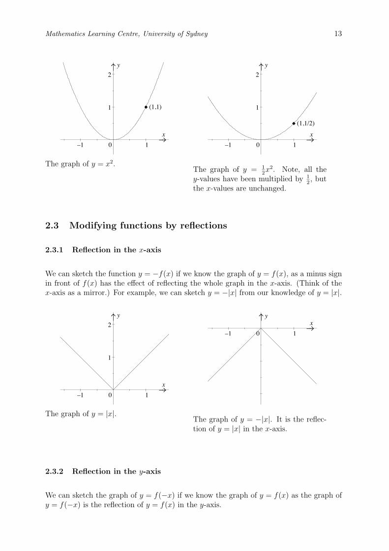
y
1
1
2
0–1
x
(1,1)
y
1
1
2
0–1
x
(1,1/2)
y
1
1
2
0–1
x
0–1
xy
1
Mathematics Learning Centre, University of Sydney 13
The graph of y = x2.The graph of y = 1
2x2. Note, all the
y-values have been multiplied by 12, but
the x-values are unchanged.
2.3 Modifying functions by reflections
2.3.1 Reflection in the x-axis
We can sketch the function y = −f(x) if we know the graph of y = f(x), as a minus signin front of f(x) has the effect of reflecting the whole graph in the x-axis. (Think of thex-axis as a mirror.) For example, we can sketch y = −|x| from our knowledge of y = |x|.
The graph of y = |x|.The graph of y = −|x|. It is the reflec-tion of y = |x| in the x-axis.
2.3.2 Reflection in the y-axis
We can sketch the graph of y = f(−x) if we know the graph of y = f(x) as the graph ofy = f(−x) is the reflection of y = f(x) in the y-axis.
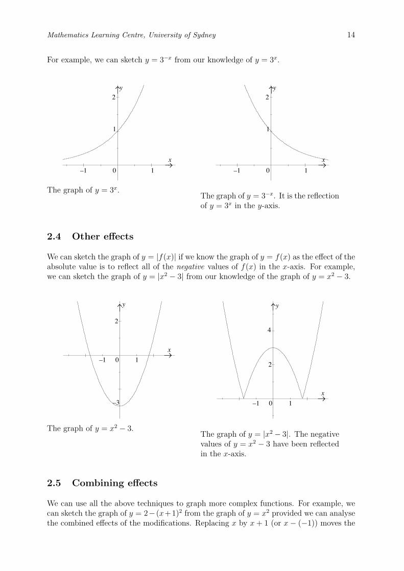
0
1
2
–1
x
y
1
0
1
2
–1
x
y
1
–3
0
2
–1
x
y
1
10
2
–1
x
y
4
Mathematics Learning Centre, University of Sydney 14
For example, we can sketch y = 3−x from our knowledge of y = 3x.
The graph of y = 3x.The graph of y = 3−x. It is the reflectionof y = 3x in the y-axis.
2.4 Other effects
We can sketch the graph of y = |f(x)| if we know the graph of y = f(x) as the effect of theabsolute value is to reflect all of the negative values of f(x) in the x-axis. For example,we can sketch the graph of y = |x2 − 3| from our knowledge of the graph of y = x2 − 3.
The graph of y = x2 − 3.The graph of y = |x2 − 3|. The negativevalues of y = x2 − 3 have been reflectedin the x-axis.
2.5 Combining effects
We can use all the above techniques to graph more complex functions. For example, wecan sketch the graph of y = 2− (x+1)2 from the graph of y = x2 provided we can analysethe combined effects of the modifications. Replacing x by x + 1 (or x − (−1)) moves the
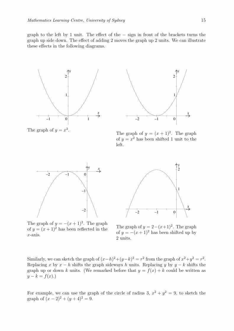
0
1
2
–1
x
y
1
x
y
0
1
2
–2 –1
–2 –1
xy
0
–1
–2
0–2 –1
x
y
1
2
Mathematics Learning Centre, University of Sydney 15
graph to the left by 1 unit. The effect of the − sign in front of the brackets turns thegraph up side down. The effect of adding 2 moves the graph up 2 units. We can illustratethese effects in the following diagrams.
The graph of y = x2.The graph of y = (x + 1)2. The graphof y = x2 has been shifted 1 unit to theleft.
The graph of y = −(x + 1)2. The graphof y = (x + 1)2 has been reflected in thex-axis.
The graph of y = 2−(x+1)2. The graphof y = −(x + 1)2 has been shifted up by2 units.
Similarly, we can sketch the graph of (x−h)2+(y−k)2 = r2 from the graph of x2+y2 = r2.Replacing x by x − h shifts the graph sideways h units. Replacing y by y − k shifts thegraph up or down k units. (We remarked before that y = f(x) + k could be written asy − k = f(x).)
For example, we can use the graph of the circle of radius 3, x2 + y2 = 9, to sketch thegraph of (x − 2)2 + (y + 4)2 = 9.
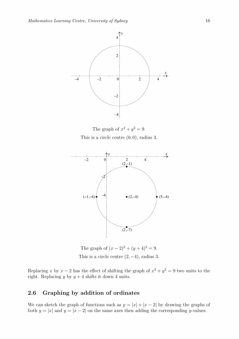
2
4
–4
y
0
–2
2 4–2
x
–4
–4
y
0
–2
2 4–2
x
(2,–4)
(2,–7)
(5,–4)(–1,–4)
(2,–1)
Mathematics Learning Centre, University of Sydney 16
The graph of x2 + y2 = 9.
This is a circle centre (0, 0), radius 3.
The graph of (x − 2)2 + (y + 4)2 = 9.
This is a circle centre (2,−4), radius 3.
Replacing x by x − 2 has the effect of shifting the graph of x2 + y2 = 9 two units to theright. Replacing y by y + 4 shifts it down 4 units.
2.6 Graphing by addition of ordinates
We can sketch the graph of functions such as y = |x| + |x − 2| by drawing the graphs ofboth y = |x| and y = |x − 2| on the same axes then adding the corresponding y-values.
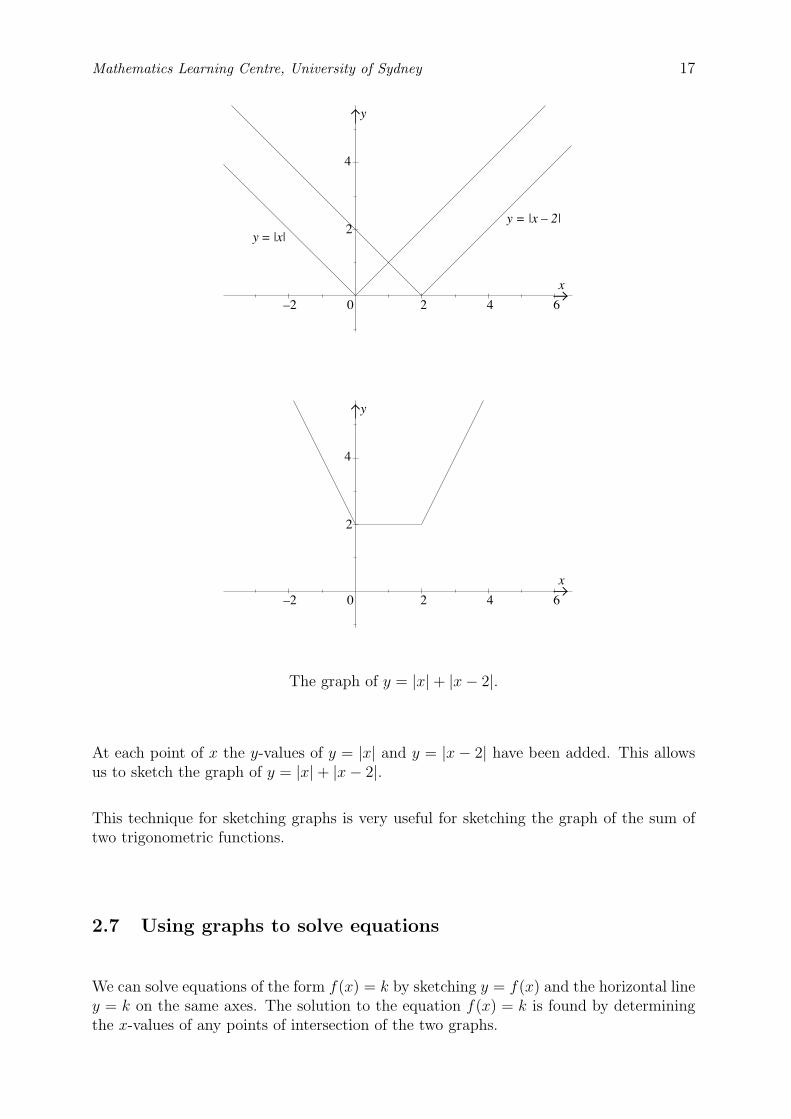
0
2
2 4 6–2
x
y
4
y = |x|
y = |x – 2|
0
2
2 4 6–2
x
y
4
Mathematics Learning Centre, University of Sydney 17
The graph of y = |x| + |x − 2|.
At each point of x the y-values of y = |x| and y = |x − 2| have been added. This allowsus to sketch the graph of y = |x| + |x − 2|.
This technique for sketching graphs is very useful for sketching the graph of the sum oftwo trigonometric functions.
2.7 Using graphs to solve equations
We can solve equations of the form f(x) = k by sketching y = f(x) and the horizontal liney = k on the same axes. The solution to the equation f(x) = k is found by determiningthe x-values of any points of intersection of the two graphs.
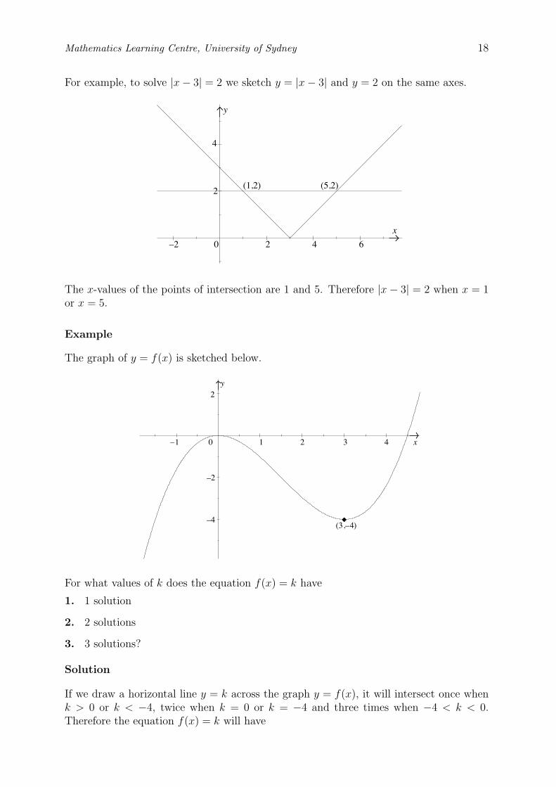
(5,2)
y
4
0
2
2 4 6–2
x
(1,2)
3 4
y
1–1
–2
–4
2
0 2 x
(3,–4)
Mathematics Learning Centre, University of Sydney 18
For example, to solve |x − 3| = 2 we sketch y = |x − 3| and y = 2 on the same axes.
The x-values of the points of intersection are 1 and 5. Therefore |x − 3| = 2 when x = 1or x = 5.
Example
The graph of y = f(x) is sketched below.
For what values of k does the equation f(x) = k have
1. 1 solution
2. 2 solutions
3. 3 solutions?
Solution
If we draw a horizontal line y = k across the graph y = f(x), it will intersect once whenk > 0 or k < −4, twice when k = 0 or k = −4 and three times when −4 < k < 0.Therefore the equation f(x) = k will have
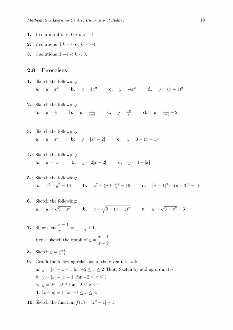
Mathematics Learning Centre, University of Sydney 19
1. 1 solution if k > 0 or k < −4
2. 2 solutions if k = 0 or k = −4
3. 3 solutions if −4 < k < 0.
2.8 Exercises
1. Sketch the following:
a. y = x2 b. y = 13x2 c. y = −x2 d. y = (x + 1)2
2. Sketch the following:
a. y = 1x
b. y = 1x−2
c. y = −2x
d. y = 1x+1
+ 2
3. Sketch the following:
a. y = x3 b. y = |x3 − 2| c. y = 3 − (x − 1)3
4. Sketch the following:
a. y = |x| b. y = 2|x − 2| c. y = 4 − |x|
5. Sketch the following:
a. x2 + y2 = 16 b. x2 + (y + 2)2 = 16 c. (x − 1)2 + (y − 3)2 = 16
6. Sketch the following:
a. y =√
9 − x2 b. y =√
9 − (x − 1)2 c. y =√
9 − x2 − 3
7. Show thatx − 1
x − 2=
1
x − 2+ 1.
Hence sketch the graph of y =x − 1
x − 2.
8. Sketch y = x+1x−1
.
9. Graph the following relations in the given interval:
a. y = |x| + x + 1 for −2 ≤ x ≤ 2 [Hint: Sketch by adding ordinates]
b. y = |x| + |x − 1| for −2 ≤ x ≤ 3
c. y = 2x + 2−x for −2 ≤ x ≤ 2
d. |x − y| = 1 for −1 ≤ x ≤ 3.
10. Sketch the function f(x) = |x2 − 1| − 1.
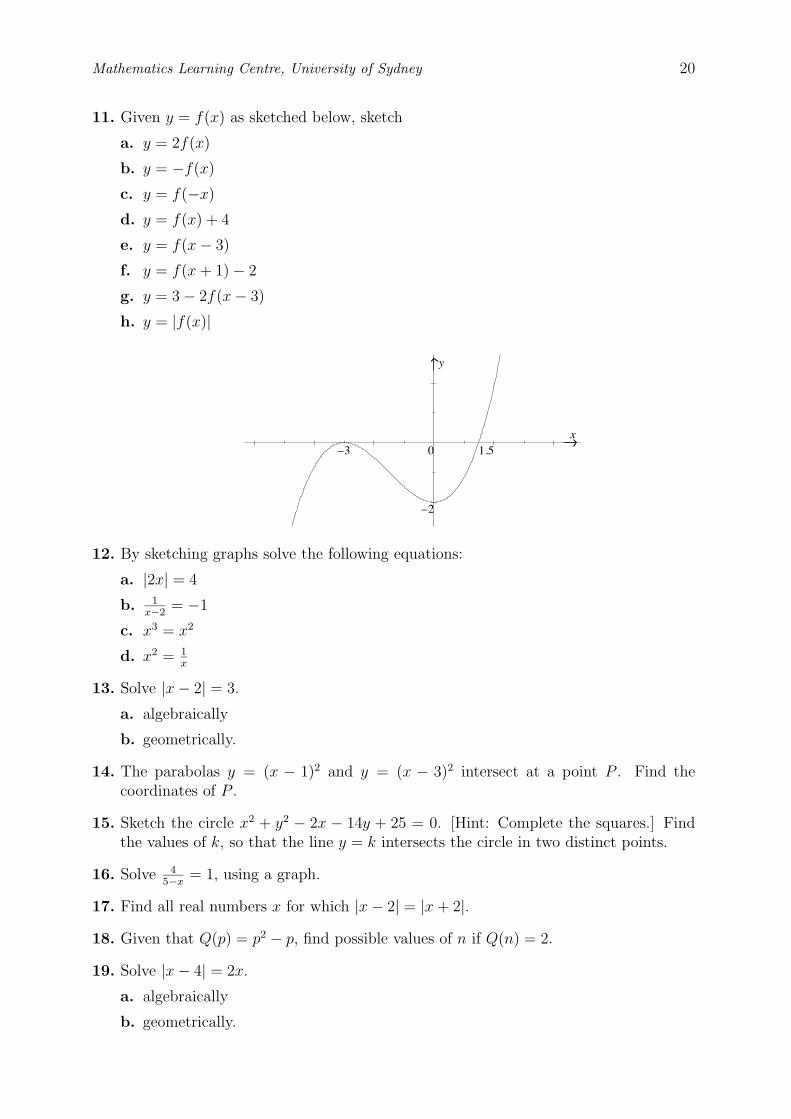
y
0x
–3 1.5
–2
Mathematics Learning Centre, University of Sydney 20
11. Given y = f(x) as sketched below, sketch
a. y = 2f(x)
b. y = −f(x)
c. y = f(−x)
d. y = f(x) + 4
e. y = f(x − 3)
f. y = f(x + 1) − 2
g. y = 3 − 2f(x − 3)
h. y = |f(x)|
12. By sketching graphs solve the following equations:
a. |2x| = 4
b. 1x−2
= −1
c. x3 = x2
d. x2 = 1x
13. Solve |x − 2| = 3.
a. algebraically
b. geometrically.
14. The parabolas y = (x − 1)2 and y = (x − 3)2 intersect at a point P . Find thecoordinates of P .
15. Sketch the circle x2 + y2 − 2x − 14y + 25 = 0. [Hint: Complete the squares.] Findthe values of k, so that the line y = k intersects the circle in two distinct points.
16. Solve 45−x
= 1, using a graph.
17. Find all real numbers x for which |x − 2| = |x + 2|.
18. Given that Q(p) = p2 − p, find possible values of n if Q(n) = 2.
19. Solve |x − 4| = 2x.
a. algebraically
b. geometrically.
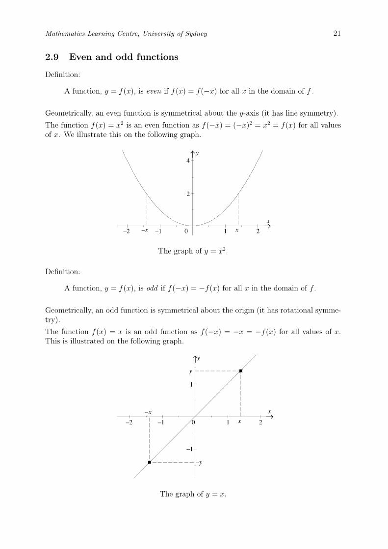
–x 0 2
x
y
1–1–2
2
4
x
y
1–1–2 x
1
–1
y
–x
0 2
x
–y
Mathematics Learning Centre, University of Sydney 21
2.9 Even and odd functions
Definition:
A function, y = f(x), is even if f(x) = f(−x) for all x in the domain of f .
Geometrically, an even function is symmetrical about the y-axis (it has line symmetry).
The function f(x) = x2 is an even function as f(−x) = (−x)2 = x2 = f(x) for all valuesof x. We illustrate this on the following graph.
The graph of y = x2.
Definition:
A function, y = f(x), is odd if f(−x) = −f(x) for all x in the domain of f .
Geometrically, an odd function is symmetrical about the origin (it has rotational symme-try).
The function f(x) = x is an odd function as f(−x) = −x = −f(x) for all values of x.This is illustrated on the following graph.
The graph of y = x.
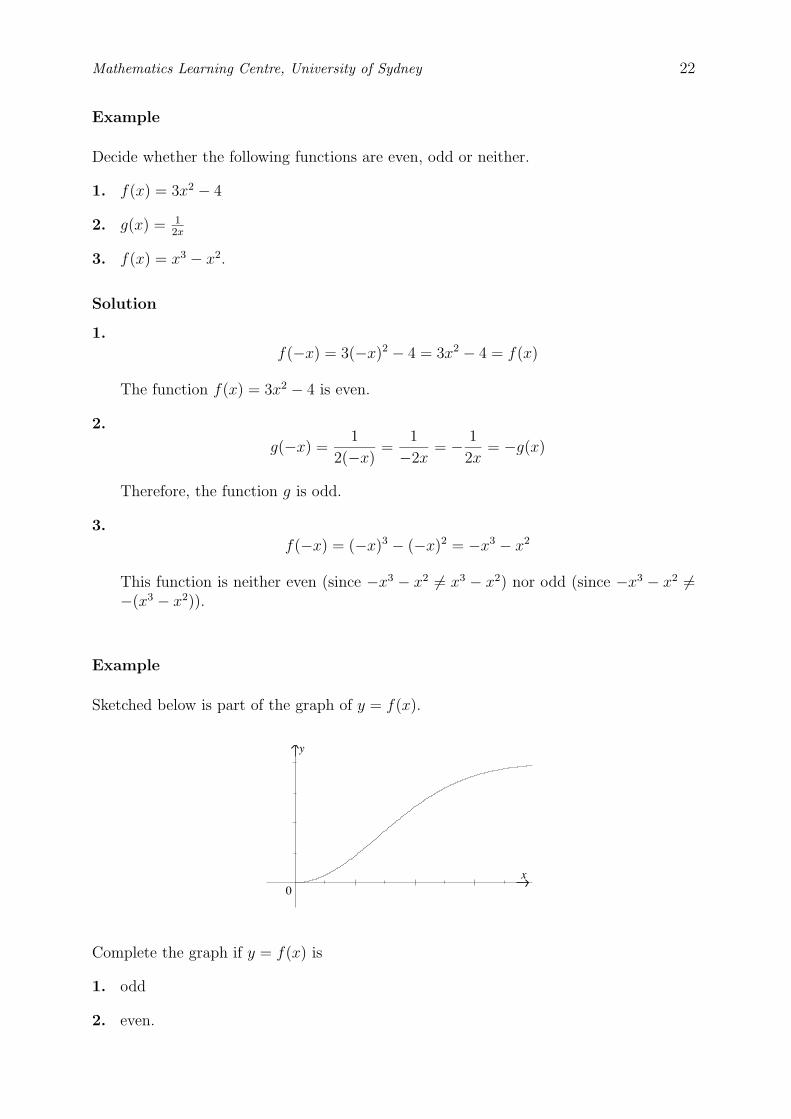
0x
y
Mathematics Learning Centre, University of Sydney 22
Example
Decide whether the following functions are even, odd or neither.
1. f(x) = 3x2 − 4
2. g(x) = 12x
3. f(x) = x3 − x2.
Solution
1.
f(−x) = 3(−x)2 − 4 = 3x2 − 4 = f(x)
The function f(x) = 3x2 − 4 is even.
2.
g(−x) =1
2(−x)=
1
−2x= − 1
2x= −g(x)
Therefore, the function g is odd.
3.
f(−x) = (−x)3 − (−x)2 = −x3 − x2
This function is neither even (since −x3 − x2 �= x3 − x2) nor odd (since −x3 − x2 �=−(x3 − x2)).
Example
Sketched below is part of the graph of y = f(x).
Complete the graph if y = f(x) is
1. odd
2. even.
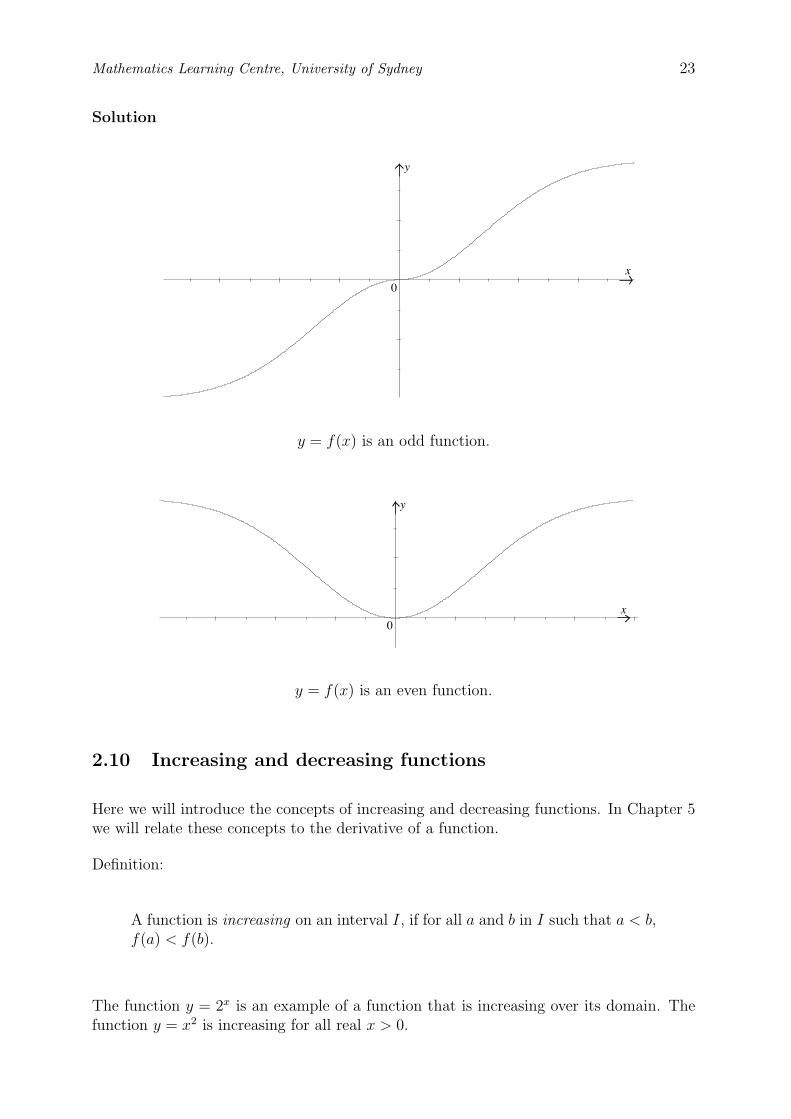
y
0
x
y
0x
Mathematics Learning Centre, University of Sydney 23
Solution
y = f(x) is an odd function.
y = f(x) is an even function.
2.10 Increasing and decreasing functions
Here we will introduce the concepts of increasing and decreasing functions. In Chapter 5we will relate these concepts to the derivative of a function.
Definition:
A function is increasing on an interval I, if for all a and b in I such that a < b,f(a) < f(b).
The function y = 2x is an example of a function that is increasing over its domain. Thefunction y = x2 is increasing for all real x > 0.
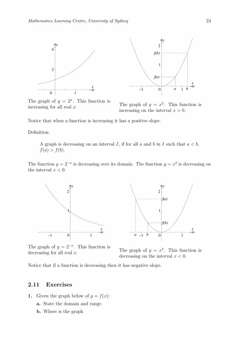
x
y
10
2
4
b
f(b)
f(a)
0
1
2
–1
x
y
1
a
0
1
2
–1
x
y
1
a
f(a)
f(b)
0
1
2
–1
x
y
1
b
Mathematics Learning Centre, University of Sydney 24
The graph of y = 2x. This function isincreasing for all real x. The graph of y = x2. This function is
increasing on the interval x > 0.
Notice that when a function is increasing it has a positive slope.
Definition:
A graph is decreasing on an interval I, if for all a and b in I such that a < b,f(a) > f(b).
The function y = 2−x is decreasing over its domain. The function y = x2 is decreasing onthe interval x < 0.
The graph of y = 2−x. This function isdecreasing for all real x. The graph of y = x2. This function is
decreasing on the interval x < 0.
Notice that if a function is decreasing then it has negative slope.
2.11 Exercises
1. Given the graph below of y = f(x):
a. State the domain and range.
b. Where is the graph
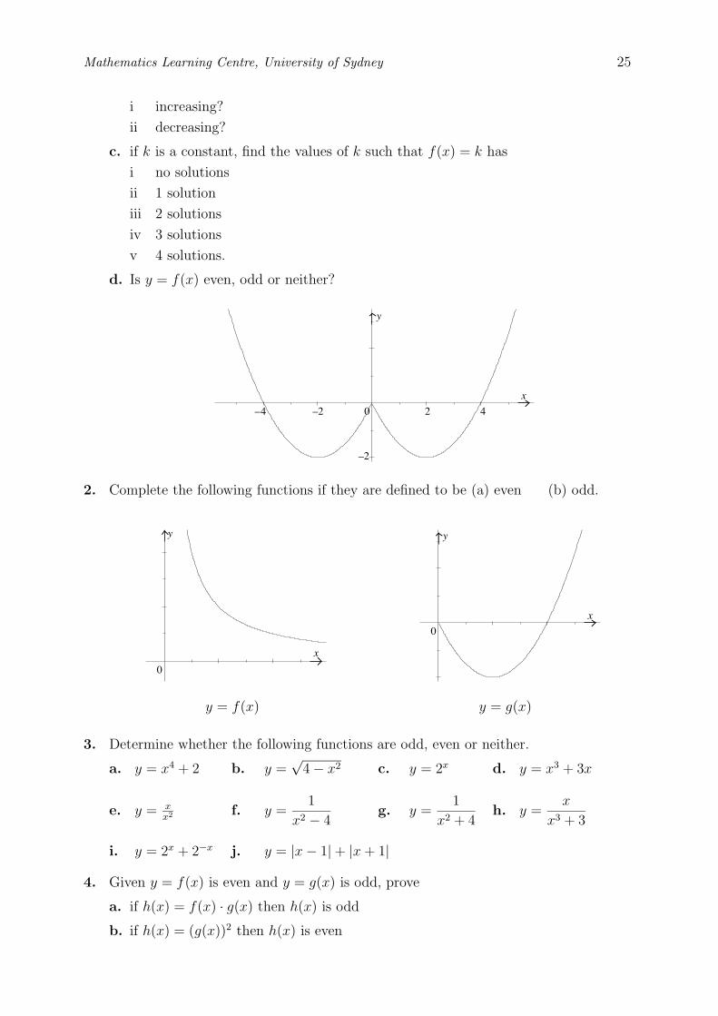
40
x
y
2–2–4
–2
x
y
0
0
x
y
Mathematics Learning Centre, University of Sydney 25
i increasing?
ii decreasing?
c. if k is a constant, find the values of k such that f(x) = k has
i no solutions
ii 1 solution
iii 2 solutions
iv 3 solutions
v 4 solutions.
d. Is y = f(x) even, odd or neither?
2. Complete the following functions if they are defined to be (a) even (b) odd.
y = f(x) y = g(x)
3. Determine whether the following functions are odd, even or neither.
a. y = x4 + 2 b. y =√
4 − x2 c. y = 2x d. y = x3 + 3x
e. y = xx2 f. y =
1
x2 − 4g. y =
1
x2 + 4h. y =
x
x3 + 3
i. y = 2x + 2−x j. y = |x − 1| + |x + 1|
4. Given y = f(x) is even and y = g(x) is odd, prove
a. if h(x) = f(x) · g(x) then h(x) is odd
b. if h(x) = (g(x))2 then h(x) is even

Mathematics Learning Centre, University of Sydney 26
c. if h(x) =f(x)
g(x), g(x) �= 0, then h(x) is odd
d. if h(x) = f(x) · (g(x))2 then h(x) is even.
5. Consider the set of all odd functions which are defined at x = 0. Can you prove thatfor every odd function in this set f(0) = 0? If not, give a counter-example.
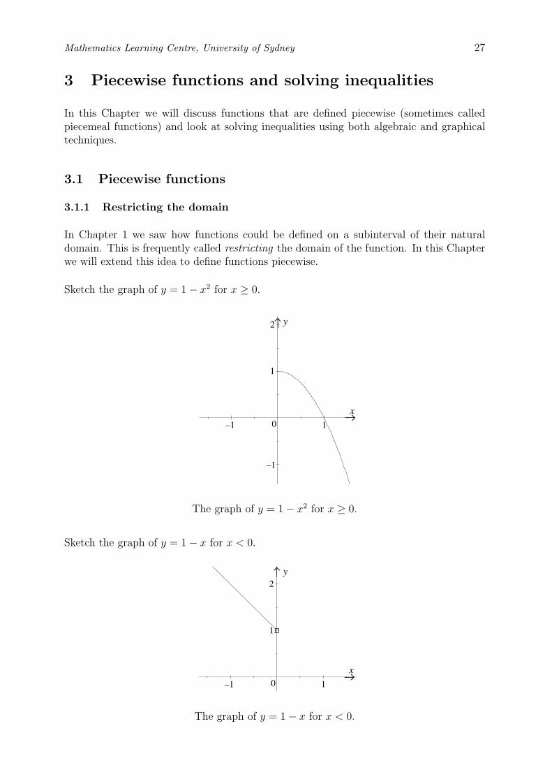
x
y
1–1
1
2
–1
0
1–1
1
2
0
x
y
Mathematics Learning Centre, University of Sydney 27
3 Piecewise functions and solving inequalities
In this Chapter we will discuss functions that are defined piecewise (sometimes calledpiecemeal functions) and look at solving inequalities using both algebraic and graphicaltechniques.
3.1 Piecewise functions
3.1.1 Restricting the domain
In Chapter 1 we saw how functions could be defined on a subinterval of their naturaldomain. This is frequently called restricting the domain of the function. In this Chapterwe will extend this idea to define functions piecewise.
Sketch the graph of y = 1 − x2 for x ≥ 0.
The graph of y = 1 − x2 for x ≥ 0.
Sketch the graph of y = 1 − x for x < 0.
The graph of y = 1 − x for x < 0.
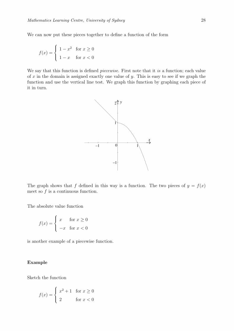
x
y
1–1
1
2
–1
0
Mathematics Learning Centre, University of Sydney 28
We can now put these pieces together to define a function of the form
f(x) =
1 − x2 for x ≥ 0
1 − x for x < 0
We say that this function is defined piecewise. First note that it is a function; each valueof x in the domain is assigned exactly one value of y. This is easy to see if we graph thefunction and use the vertical line test. We graph this function by graphing each piece ofit in turn.
The graph shows that f defined in this way is a function. The two pieces of y = f(x)meet so f is a continuous function.
The absolute value function
f(x) =
x for x ≥ 0
−x for x < 0
is another example of a piecewise function.
Example
Sketch the function
f(x) =
x2 + 1 for x ≥ 0
2 for x < 0
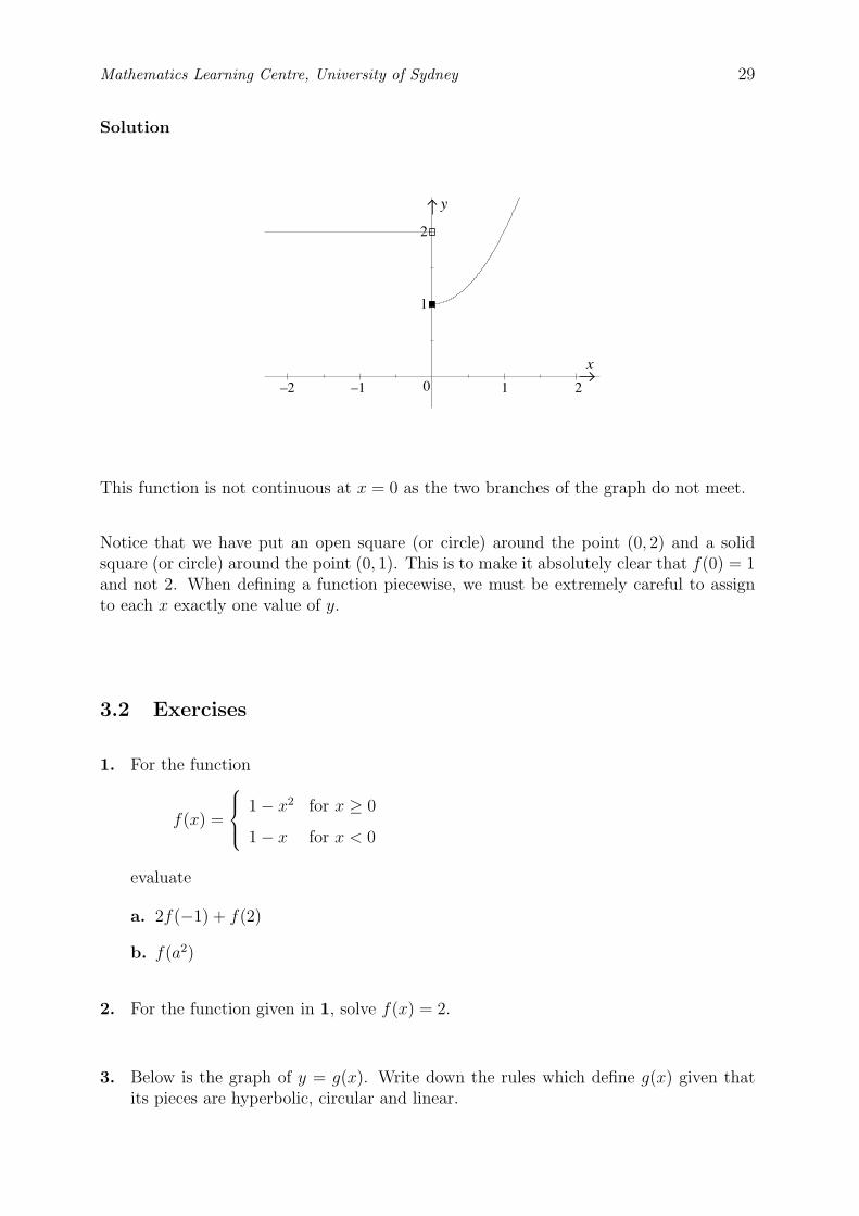
–1
1
2
0
x
y
1 2–2
Mathematics Learning Centre, University of Sydney 29
Solution
This function is not continuous at x = 0 as the two branches of the graph do not meet.
Notice that we have put an open square (or circle) around the point (0, 2) and a solidsquare (or circle) around the point (0, 1). This is to make it absolutely clear that f(0) = 1and not 2. When defining a function piecewise, we must be extremely careful to assignto each x exactly one value of y.
3.2 Exercises
1. For the function
f(x) =
1 − x2 for x ≥ 0
1 − x for x < 0
evaluate
a. 2f(−1) + f(2)
b. f(a2)
2. For the function given in 1, solve f(x) = 2.
3. Below is the graph of y = g(x). Write down the rules which define g(x) given thatits pieces are hyperbolic, circular and linear.
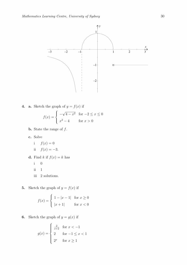
–2–3
1
–1
–2
x
y
1–1 2 3
Mathematics Learning Centre, University of Sydney 30
4. a. Sketch the graph of y = f(x) if
f(x) =
−√
4 − x2 for −2 ≤ x ≤ 0
x2 − 4 for x > 0
b. State the range of f .
c. Solve
i f(x) = 0
ii f(x) = −3.
d. Find k if f(x) = k has
i 0
ii 1
iii 2 solutions.
5. Sketch the graph of y = f(x) if
f(x) =
1 − |x − 1| for x ≥ 0
|x + 1| for x < 0
6. Sketch the graph of y = g(x) if
g(x) =
2x+2
for x < −1
2 for −1 ≤ x < 1
2x for x ≥ 1
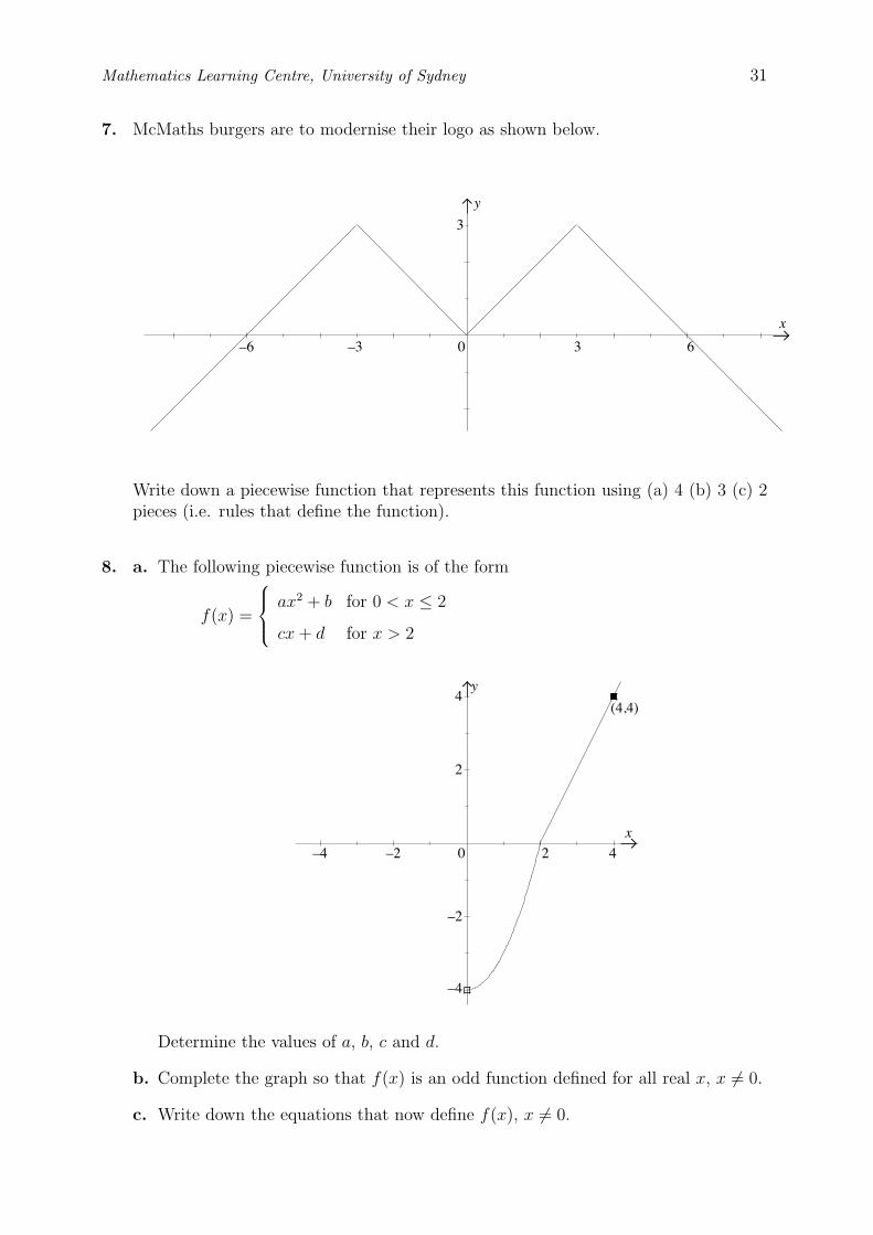
30 6–3–6
3
x
y
(4,4)
x
y
–4 0
–2
–4
2
4
2 4–2
Mathematics Learning Centre, University of Sydney 31
7. McMaths burgers are to modernise their logo as shown below.
Write down a piecewise function that represents this function using (a) 4 (b) 3 (c) 2pieces (i.e. rules that define the function).
8. a. The following piecewise function is of the form
f(x) =
ax2 + b for 0 < x ≤ 2
cx + d for x > 2
Determine the values of a, b, c and d.
b. Complete the graph so that f(x) is an odd function defined for all real x, x �= 0.
c. Write down the equations that now define f(x), x �= 0.
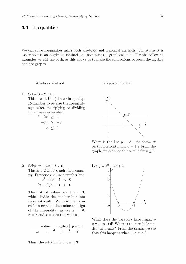
3
2
x
(1,1)
y
10
0 1 2 3 4–1
positive negative positive
x
y
1 30
3
1
Mathematics Learning Centre, University of Sydney 32
3.3 Inequalities
We can solve inequalities using both algebraic and graphical methods. Sometimes it iseasier to use an algebraic method and sometimes a graphical one. For the followingexamples we will use both, as this allows us to make the connections between the algebraand the graphs.
Algebraic method Graphical method
1. Solve 3 − 2x ≥ 1.This is a (2 Unit) linear inequality.Remember to reverse the inequalitysign when multiplying or dividingby a negative number.
3 − 2x ≥ 1
−2x ≥ −2
x ≤ 1
When is the line y = 3 − 2x above oron the horizontal line y = 1 ? From thegraph, we see that this is true for x ≤ 1.
2. Solve x2 − 4x + 3 < 0.This is a (2 Unit) quadratic inequal-ity. Factorise and use a number line.
x2 − 4x + 3 < 0
(x − 3)(x − 1) < 0
The critical values are 1 and 3,which divide the number line intothree intervals. We take points ineach interval to determine the signof the inequality; eg use x = 0,x = 2 and x = 4 as test values.
Thus, the solution is 1 < x < 3.
Let y = x2 − 4x + 3.
When does the parabola have negativey-values? OR When is the parabola un-der the x-axis? From the graph, we seethat this happens when 1 < x < 3.
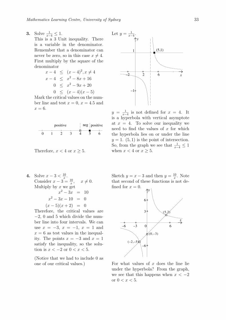
positive
0 1 2 3 4 5 6
positive neg
(5,1)
x2 6
1
–1
–2
y
–6 –3 0 6
3
6
–6
(5,2)
(–2,–5)
(0,–3)
x
y
Mathematics Learning Centre, University of Sydney 33
3. Solve 1x−4
≤ 1.This is a 3 Unit inequality. Thereis a variable in the denominator.Remember that a denominator cannever be zero, so in this case x �= 4.First multiply by the square of thedenominator
x − 4 ≤ (x − 4)2, x �= 4
x − 4 ≤ x2 − 8x + 16
0 ≤ x2 − 9x + 20
0 ≤ (x − 4)(x − 5)Mark the critical values on the num-ber line and test x = 0, x = 4.5 andx = 6.
Therefore, x < 4 or x ≥ 5.
Let y = 1x−4
.
y = 1x−4
is not defined for x = 4. Itis a hyperbola with vertical asymptoteat x = 4. To solve our inequality weneed to find the values of x for whichthe hyperbola lies on or under the liney = 1. (5, 1) is the point of intersection.So, from the graph we see that 1
x−4≤ 1
when x < 4 or x ≥ 5.
4. Solve x − 3 < 10x
.Consider x − 3 = 10
x, x �= 0.
Multiply by x we getx2 − 3x = 10
x2 − 3x − 10 = 0
(x − 5)(x + 2) = 0Therefore, the critical values are−2, 0 and 5 which divide the num-ber line into four intervals. We canuse x = −3, x = −1, x = 1 andx = 6 as test values in the inequal-ity. The points x = −3 and x = 1satisfy the inequality, so the solu-tion is x < −2 or 0 < x < 5.
(Notice that we had to include 0 asone of our critical values.)
Sketch y = x− 3 and then y = 10x
. Notethat second of these functions is not de-fined for x = 0.
For what values of x does the line lieunder the hyperbola? From the graph,we see that this happens when x < −2or 0 < x < 5.
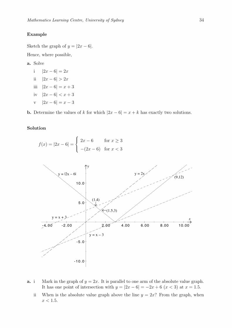
2.00 4.00 6.00 8.00 10.00-2 .00-4 .00
-5 .0
-10 .0
5.0
10.0
y = |2x – 6|
y = x – 3
y = x + 3
y = 2x(9,12)
(1,4)
(1.5,3)
y
x
Mathematics Learning Centre, University of Sydney 34
Example
Sketch the graph of y = |2x − 6|.Hence, where possible,
a. Solve
i |2x − 6| = 2x
ii |2x − 6| > 2x
iii |2x − 6| = x + 3
iv |2x − 6| < x + 3
v |2x − 6| = x − 3
b. Determine the values of k for which |2x − 6| = x + k has exactly two solutions.
Solution
f(x) = |2x − 6| =
2x − 6 for x ≥ 3
−(2x − 6) for x < 3
a. i Mark in the graph of y = 2x. It is parallel to one arm of the absolute value graph.It has one point of intersection with y = |2x − 6| = −2x + 6 (x < 3) at x = 1.5.
ii When is the absolute value graph above the line y = 2x? From the graph, whenx < 1.5.
Mathematics Learning Centre, University of Sydney 35
iii y = x + 3 intersects y = |2x − 6| twice.
To solve |2x − 6| = x + 3, take |2x − 6| = 2x − 6 = x + 3 when x ≥ 3. This givesus the solution x = 9. Then take |2x − 6| = −2x + 6 = x + 3 when x < 3 whichgives us the solution x = 1.
iv When is the absolute value graph below the line y = x + 3?
From the graph, 1 < x < 9.
v y = x − 3 intersects the absolute value graph at x = 3 only.
b. k represents the y-intercept of the line y = x + k. When k = −3, there is one point ofintersection. (See (a) (v) above). For k > −3, lines of the form y = x + k will havetwo points of intersection. Hence |2x− 6| = x + k will have two solutions for k > −3.
3.4 Exercises
1. Solve
a. x2 ≤ 4x
b. 4pp+3
≤ 1
c. 79−x2 > −1
2. a. Sketch the graph of y = 4x(x − 3).
b. Hence solve 4x(x − 3) ≤ 0.
3. a. Find the points of intersection of the graphs y = 5 − x and y = 4x.
b. On the same set of axes, sketch the graphs of y = 5 − x and y = 4x.
c. Using part (ii), or otherwise, write down all the values of x for which
5 − x >4
x
4. a. Sketch the graph of y = 2x.
b. Solve 2x < 12.
c. Suppose 0 < a < b and consider the points A(a, 2a) and B(b, 2b) on the graph ofy = 2x. Find the coordinates of the midpoint M of the segment AB.
Explain why2a + 2b
2> 2
a+b2
5. a. Sketch the graphs of y = x and y = |x − 5| on the same diagram.
b. Solve |x − 5| > x.
c. For what values of m does mx = |x − 5| have exactly
i two solutions
ii no solutions
6. Solve 5x2 − 6x − 3 ≤ |8x|.
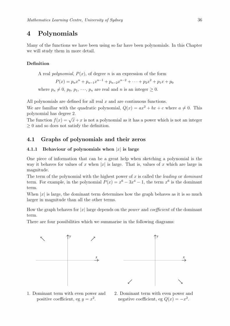
x
y y
x
Mathematics Learning Centre, University of Sydney 36
4 Polynomials
Many of the functions we have been using so far have been polynomials. In this Chapterwe will study them in more detail.
Definition
A real polynomial, P (x), of degree n is an expression of the form
P (x) = pnxn + pn−1x
n−1 + pn−2xn−2 + · · · + p2x
2 + p1x + p0
where pn �= 0, p0, p1, · · ·, pn are real and n is an integer ≥ 0.
All polynomials are defined for all real x and are continuous functions.
We are familiar with the quadratic polynomial, Q(x) = ax2 + bx + c where a �= 0. Thispolynomial has degree 2.
The function f(x) =√
x+x is not a polynomial as it has a power which is not an integer≥ 0 and so does not satisfy the definition.
4.1 Graphs of polynomials and their zeros
4.1.1 Behaviour of polynomials when |x| is large
One piece of information that can be a great help when sketching a polynomial is theway it behaves for values of x when |x| is large. That is, values of x which are large inmagnitude.
The term of the polynomial with the highest power of x is called the leading or dominantterm. For example, in the polynomial P (x) = x6 − 3x4 − 1, the term x6 is the dominantterm.
When |x| is large, the dominant term determines how the graph behaves as it is so muchlarger in magnitude than all the other terms.
How the graph behaves for |x| large depends on the power and coefficient of the dominantterm.
There are four possibilities which we summarise in the following diagrams:
1. Dominant term with even power andpositive coefficient, eg y = x2.
2. Dominant term with even power andnegative coefficient, eg Q(x) = −x2.
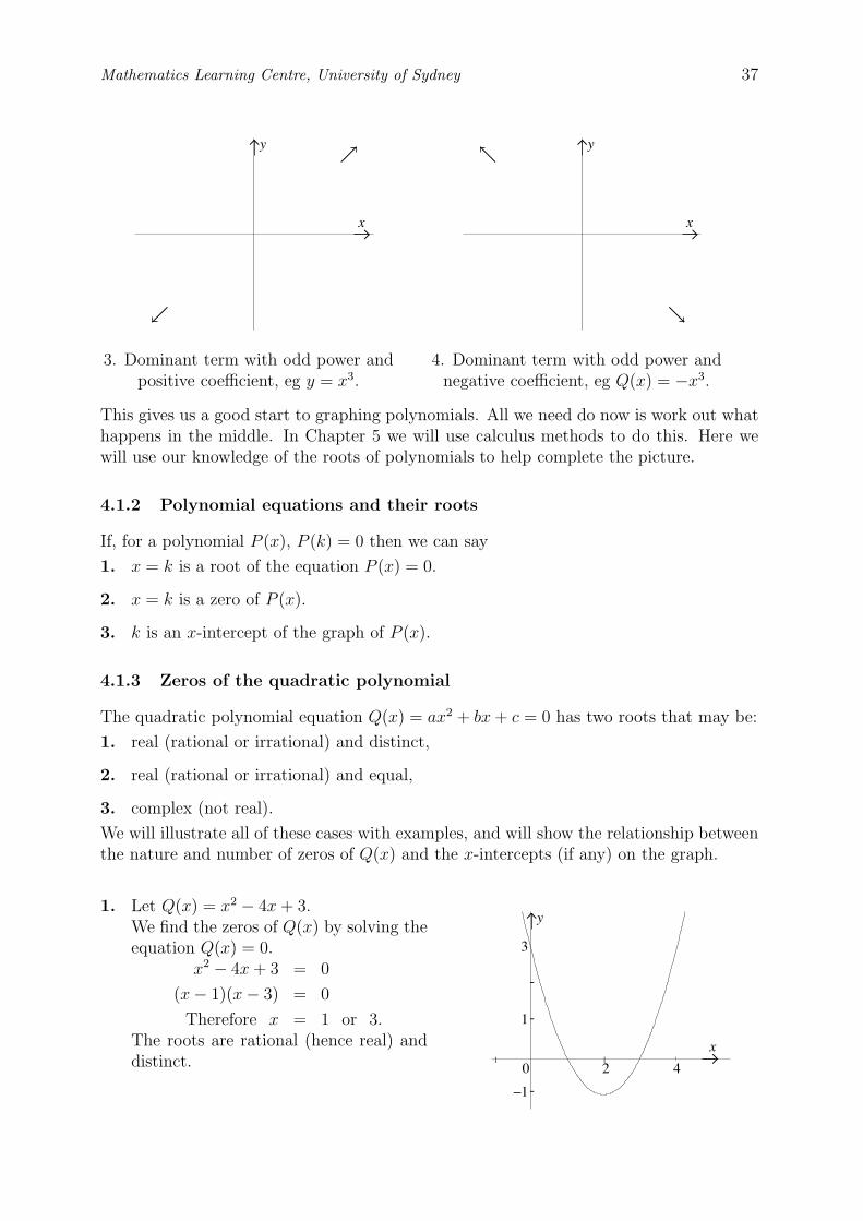
y
x
y
x
-
x
y
2 40
1
3
–1
||
-
-
Mathematics Learning Centre, University of Sydney 37
3. Dominant term with odd power andpositive coefficient, eg y = x3.
4. Dominant term with odd power andnegative coefficient, eg Q(x) = −x3.
This gives us a good start to graphing polynomials. All we need do now is work out whathappens in the middle. In Chapter 5 we will use calculus methods to do this. Here wewill use our knowledge of the roots of polynomials to help complete the picture.
4.1.2 Polynomial equations and their roots
If, for a polynomial P (x), P (k) = 0 then we can say
1. x = k is a root of the equation P (x) = 0.
2. x = k is a zero of P (x).
3. k is an x-intercept of the graph of P (x).
4.1.3 Zeros of the quadratic polynomial
The quadratic polynomial equation Q(x) = ax2 + bx + c = 0 has two roots that may be:
1. real (rational or irrational) and distinct,
2. real (rational or irrational) and equal,
3. complex (not real).
We will illustrate all of these cases with examples, and will show the relationship betweenthe nature and number of zeros of Q(x) and the x-intercepts (if any) on the graph.
1. Let Q(x) = x2 − 4x + 3.We find the zeros of Q(x) by solving theequation Q(x) = 0.
x2 − 4x + 3 = 0
(x − 1)(x − 3) = 0
Therefore x = 1 or 3.The roots are rational (hence real) anddistinct.
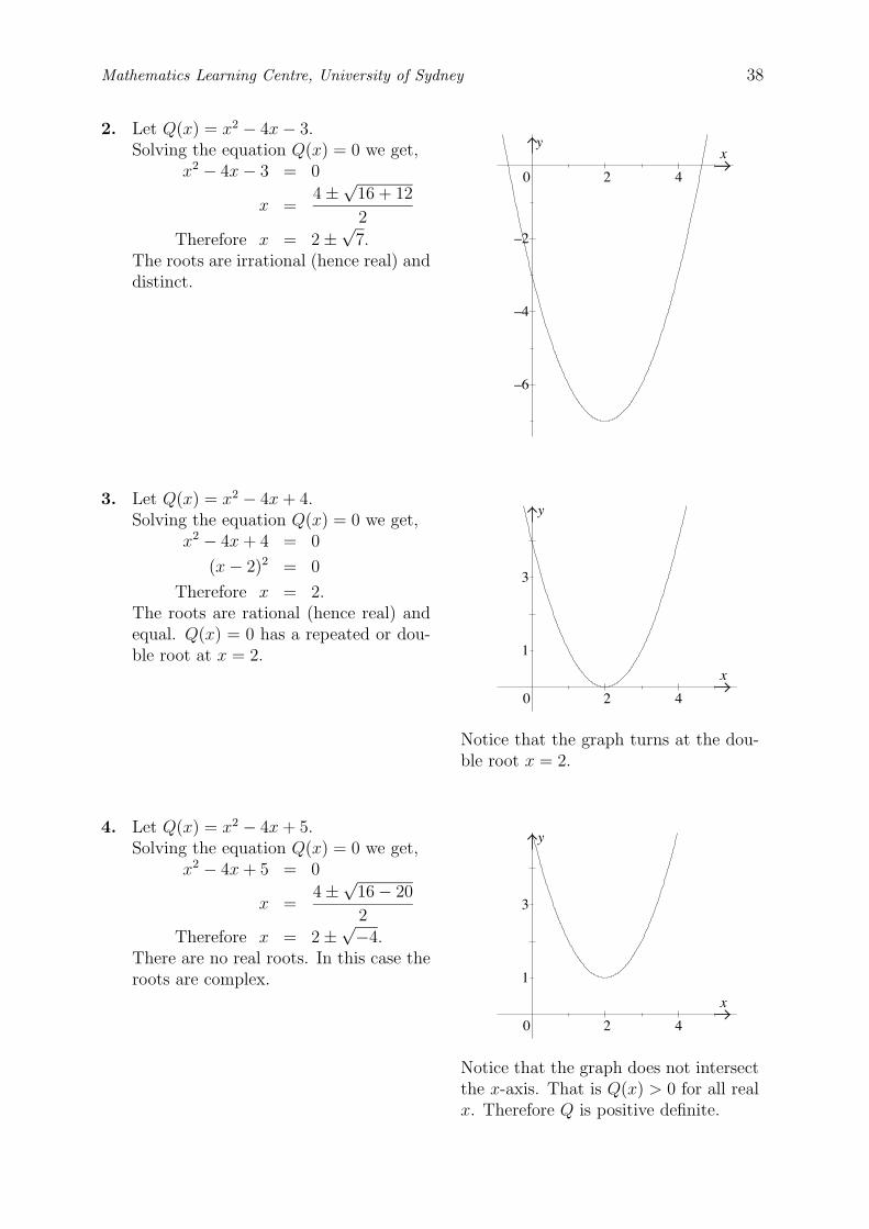
y
2 40
–6
–4
–2
x
x
y
2 40
1
3
x
y
2 40
1
3
Mathematics Learning Centre, University of Sydney 38
2. Let Q(x) = x2 − 4x − 3.Solving the equation Q(x) = 0 we get,
x2 − 4x − 3 = 0
x =4 ±
√16 + 12
2
Therefore x = 2 ±√
7.The roots are irrational (hence real) anddistinct.
3. Let Q(x) = x2 − 4x + 4.Solving the equation Q(x) = 0 we get,
x2 − 4x + 4 = 0
(x − 2)2 = 0
Therefore x = 2.The roots are rational (hence real) andequal. Q(x) = 0 has a repeated or dou-ble root at x = 2.
Notice that the graph turns at the dou-ble root x = 2.
4. Let Q(x) = x2 − 4x + 5.Solving the equation Q(x) = 0 we get,
x2 − 4x + 5 = 0
x =4 ±
√16 − 20
2Therefore x = 2 ±
√−4.
There are no real roots. In this case theroots are complex.
Notice that the graph does not intersectthe x-axis. That is Q(x) > 0 for all realx. Therefore Q is positive definite.
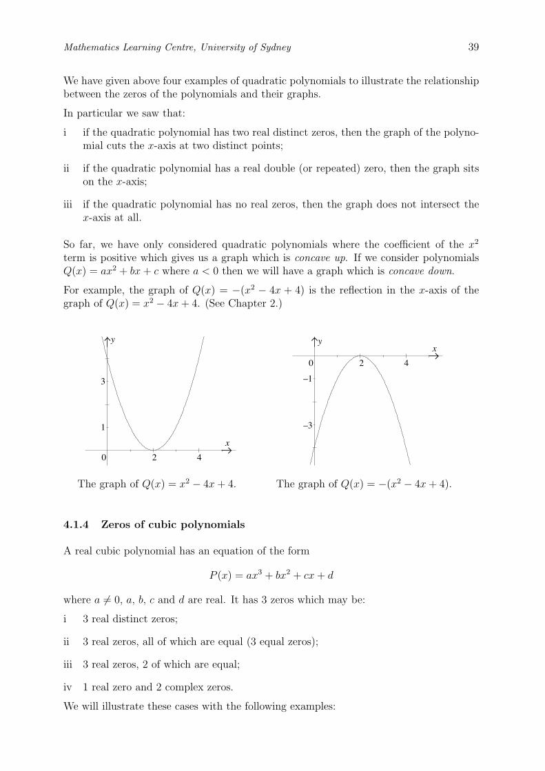
x
y
2 40
1
3
2 40
xy
–1
–3
Mathematics Learning Centre, University of Sydney 39
We have given above four examples of quadratic polynomials to illustrate the relationshipbetween the zeros of the polynomials and their graphs.
In particular we saw that:
i if the quadratic polynomial has two real distinct zeros, then the graph of the polyno-mial cuts the x-axis at two distinct points;
ii if the quadratic polynomial has a real double (or repeated) zero, then the graph sitson the x-axis;
iii if the quadratic polynomial has no real zeros, then the graph does not intersect thex-axis at all.
So far, we have only considered quadratic polynomials where the coefficient of the x2
term is positive which gives us a graph which is concave up. If we consider polynomialsQ(x) = ax2 + bx + c where a < 0 then we will have a graph which is concave down.
For example, the graph of Q(x) = −(x2 − 4x + 4) is the reflection in the x-axis of thegraph of Q(x) = x2 − 4x + 4. (See Chapter 2.)
The graph of Q(x) = x2 − 4x + 4. The graph of Q(x) = −(x2 − 4x + 4).
4.1.4 Zeros of cubic polynomials
A real cubic polynomial has an equation of the form
P (x) = ax3 + bx2 + cx + d
where a �= 0, a, b, c and d are real. It has 3 zeros which may be:
i 3 real distinct zeros;
ii 3 real zeros, all of which are equal (3 equal zeros);
iii 3 real zeros, 2 of which are equal;
iv 1 real zero and 2 complex zeros.
We will illustrate these cases with the following examples:
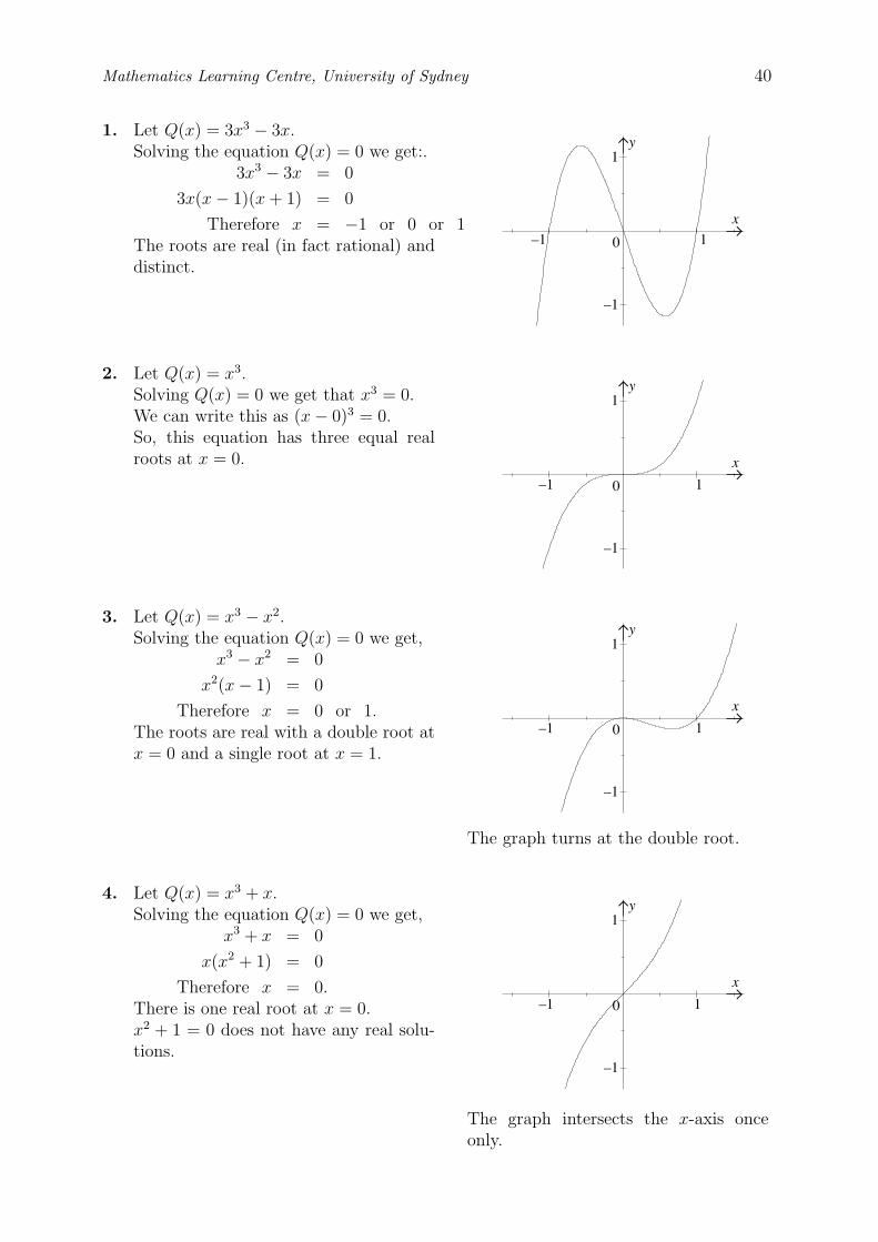
–1
0
x
1
1–1
y
y
–1
0
x
1
1–1
y
–1
0
x
1
1–1
y
–1
0
x
1
1–1
Mathematics Learning Centre, University of Sydney 40
1. Let Q(x) = 3x3 − 3x.Solving the equation Q(x) = 0 we get:.
3x3 − 3x = 0
3x(x − 1)(x + 1) = 0
Therefore x = −1 or 0 or 1The roots are real (in fact rational) anddistinct.
2. Let Q(x) = x3.Solving Q(x) = 0 we get that x3 = 0.We can write this as (x − 0)3 = 0.So, this equation has three equal realroots at x = 0.
3. Let Q(x) = x3 − x2.Solving the equation Q(x) = 0 we get,
x3 − x2 = 0
x2(x − 1) = 0
Therefore x = 0 or 1.The roots are real with a double root atx = 0 and a single root at x = 1.
The graph turns at the double root.
4. Let Q(x) = x3 + x.Solving the equation Q(x) = 0 we get,
x3 + x = 0
x(x2 + 1) = 0
Therefore x = 0.There is one real root at x = 0.x2 + 1 = 0 does not have any real solu-tions.
The graph intersects the x-axis onceonly.
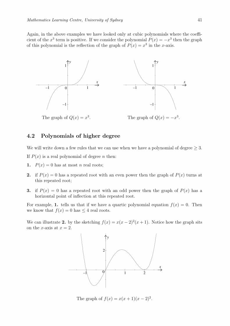
y
–1
0
x
1
1–1
y
–1
0
x
1
1–1
–1
2
2
x
y
10
Mathematics Learning Centre, University of Sydney 41
Again, in the above examples we have looked only at cubic polynomials where the coeffi-cient of the x3 term is positive. If we consider the polynomial P (x) = −x3 then the graphof this polynomial is the reflection of the graph of P (x) = x3 in the x-axis.
The graph of Q(x) = x3. The graph of Q(x) = −x3.
4.2 Polynomials of higher degree
We will write down a few rules that we can use when we have a polynomial of degree ≥ 3.
If P (x) is a real polynomial of degree n then:
1. P (x) = 0 has at most n real roots;
2. if P (x) = 0 has a repeated root with an even power then the graph of P (x) turns atthis repeated root;
3. if P (x) = 0 has a repeated root with an odd power then the graph of P (x) has ahorizontal point of inflection at this repeated root.
For example, 1. tells us that if we have a quartic polynomial equation f(x) = 0. Thenwe know that f(x) = 0 has ≤ 4 real roots.
We can illustrate 2. by the sketching f(x) = x(x− 2)2(x + 1). Notice how the graph sitson the x-axis at x = 2.
The graph of f(x) = x(x + 1)(x − 2)2.
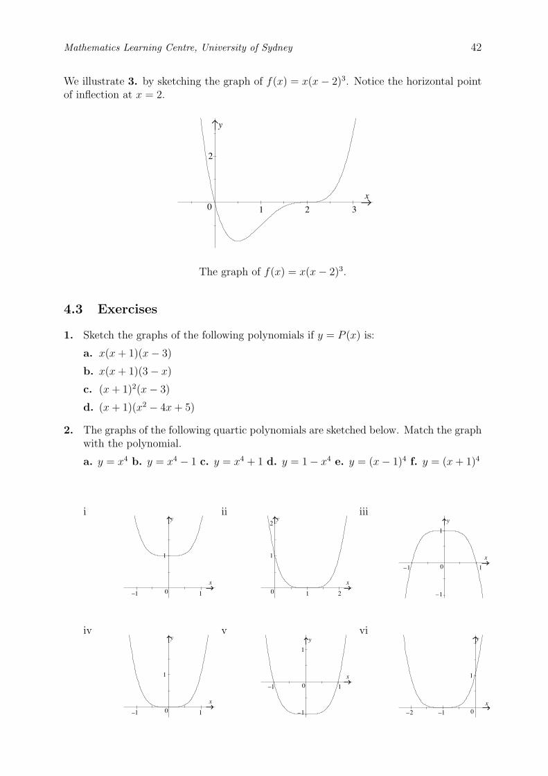
y
10 3
2
2
x
y
0
x
1
1–1 1
y
0
x
2
1
2
1–1
y
0
x
1
–1
y
0
x
1
1–1
y
0
x
1
–1
1–1
y
0x
1
–1–2
Mathematics Learning Centre, University of Sydney 42
We illustrate 3. by sketching the graph of f(x) = x(x − 2)3. Notice the horizontal pointof inflection at x = 2.
The graph of f(x) = x(x − 2)3.
4.3 Exercises
1. Sketch the graphs of the following polynomials if y = P (x) is:
a. x(x + 1)(x − 3)
b. x(x + 1)(3 − x)
c. (x + 1)2(x − 3)
d. (x + 1)(x2 − 4x + 5)
2. The graphs of the following quartic polynomials are sketched below. Match the graphwith the polynomial.
a. y = x4 b. y = x4 − 1 c. y = x4 + 1 d. y = 1 − x4 e. y = (x − 1)4 f. y = (x + 1)4
i ii iii
iv v vi
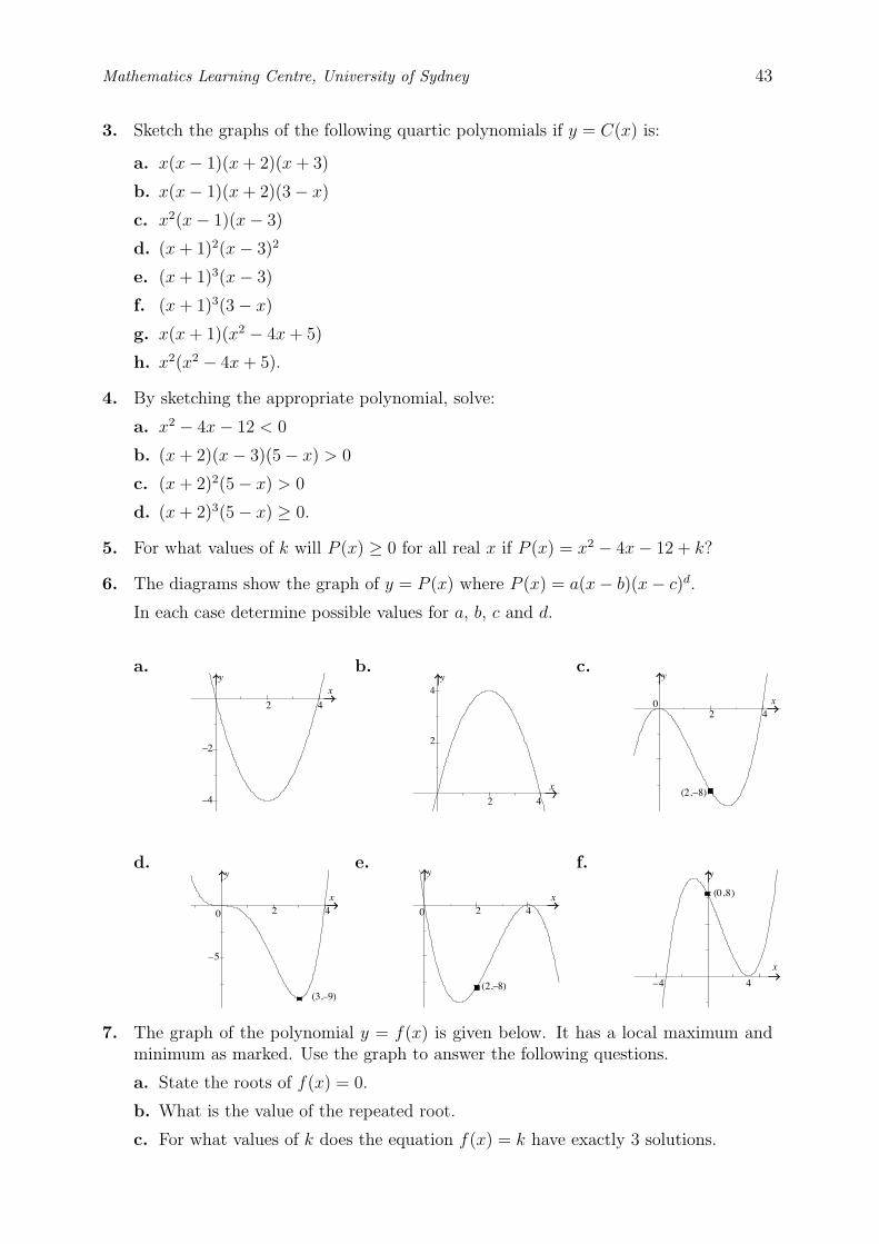
2 4
–2
–4
xy
2 4
2
4
x
y y
2 4
(2,–8)
0 x
2 40
x
y
(3,–9)
–5
0
x
y
2 4
(2,–8)
y
x
4–4
(0,8)
Mathematics Learning Centre, University of Sydney 43
3. Sketch the graphs of the following quartic polynomials if y = C(x) is:
a. x(x − 1)(x + 2)(x + 3)
b. x(x − 1)(x + 2)(3 − x)
c. x2(x − 1)(x − 3)
d. (x + 1)2(x − 3)2
e. (x + 1)3(x − 3)
f. (x + 1)3(3 − x)
g. x(x + 1)(x2 − 4x + 5)
h. x2(x2 − 4x + 5).
4. By sketching the appropriate polynomial, solve:
a. x2 − 4x − 12 < 0
b. (x + 2)(x − 3)(5 − x) > 0
c. (x + 2)2(5 − x) > 0
d. (x + 2)3(5 − x) ≥ 0.
5. For what values of k will P (x) ≥ 0 for all real x if P (x) = x2 − 4x − 12 + k?
6. The diagrams show the graph of y = P (x) where P (x) = a(x − b)(x − c)d.
In each case determine possible values for a, b, c and d.
a. b. c.
d. e. f.
7. The graph of the polynomial y = f(x) is given below. It has a local maximum andminimum as marked. Use the graph to answer the following questions.
a. State the roots of f(x) = 0.
b. What is the value of the repeated root.
c. For what values of k does the equation f(x) = k have exactly 3 solutions.
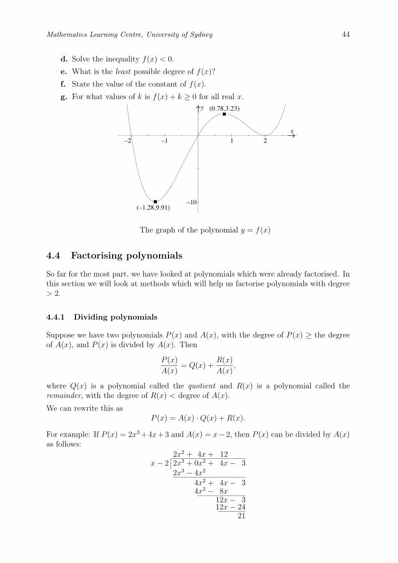
–10
2
x
y
1–2
(–1.28,9.91)
(0.78,3.23)
–1
Mathematics Learning Centre, University of Sydney 44
d. Solve the inequality f(x) < 0.
e. What is the least possible degree of f(x)?
f. State the value of the constant of f(x).
g. For what values of k is f(x) + k ≥ 0 for all real x.
The graph of the polynomial y = f(x)
4.4 Factorising polynomials
So far for the most part, we have looked at polynomials which were already factorised. Inthis section we will look at methods which will help us factorise polynomials with degree> 2.
4.4.1 Dividing polynomials
Suppose we have two polynomials P (x) and A(x), with the degree of P (x) ≥ the degreeof A(x), and P (x) is divided by A(x). Then
P (x)
A(x)= Q(x) +
R(x)
A(x),
where Q(x) is a polynomial called the quotient and R(x) is a polynomial called theremainder, with the degree of R(x) < degree of A(x).
We can rewrite this asP (x) = A(x) · Q(x) + R(x).
For example: If P (x) = 2x3 +4x+3 and A(x) = x−2, then P (x) can be divided by A(x)as follows:
2x2 + 4x + 12x − 2 2x3 + 0x2 + 4x − 3
2x3 − 4x2
4x2 + 4x − 34x2 − 8x
12x − 312x − 24
21
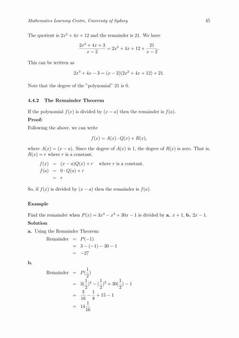
Mathematics Learning Centre, University of Sydney 45
The quotient is 2x2 + 4x + 12 and the remainder is 21. We have
2x3 + 4x + 3
x − 2= 2x2 + 4x + 12 +
21
x − 2.
This can be written as
2x3 + 4x − 3 = (x − 2)(2x2 + 4x + 12) + 21.
Note that the degree of the ”polynomial” 21 is 0.
4.4.2 The Remainder Theorem
If the polynomial f(x) is divided by (x − a) then the remainder is f(a).
Proof:
Following the above, we can write
f(x) = A(x) · Q(x) + R(x),
where A(x) = (x − a). Since the degree of A(x) is 1, the degree of R(x) is zero. That is,R(x) = r where r is a constant.
f(x) = (x − a)Q(x) + r where r is a constant.
f(a) = 0 · Q(a) + r
= r
So, if f(x) is divided by (x − a) then the remainder is f(a).
Example
Find the remainder when P (x) = 3x4 − x3 + 30x − 1 is divided by a. x + 1, b. 2x − 1.
Solution
a. Using the Remainder Theorem:
Remainder = P (−1)
= 3 − (−1) − 30 − 1
= −27
b.
Remainder = P (1
2)
= 3(1
2)4 − (
1
2)3 + 30(
1
2) − 1
=3
16− 1
8+ 15 − 1
= 141
16

Mathematics Learning Centre, University of Sydney 46
Example
When the polynomial f(x) is divided by x2 − 4, the remainder is 5x + 6. What is theremainder when f(x) is divided by (x − 2)?
Solution
Write f(x) = (x2 − 4) · q(x) + (5x + 6). Then
Remainder = f(2)
= 0 · q(2) + 16
= 16
A consequence of the Remainder Theorem is the Factor Theorem which we state below.
4.4.3 The Factor Theorem
If x = a is a zero of f(x), that is f(a) = 0, then (x − a) is a factor of f(x) and f(x) maybe written as
f(x) = (x − a)q(x)
for some polynomial q(x).
Also, if (x− a) and (x− b) are factors of f(x) then (x− a)(x− b) is a factor of f(x) and
f(x) = (x − a)(x − b) · Q(x)
for some polynomial Q(x).
Another useful fact about zeros of polynomials is given below for a polynomial of degree3.
If a (real) polynomialP (x) = ax3 + bx2 + cx + d,
where a �= 0, a, b, c and d are real, has exactly 3 real zeros α, β and γ, then
P (x) = a(x − α)(x − β)(x − γ) (1)
Furthermore, by expanding the right hand side of (1) and equating coefficients we get:
i
α + β + γ = − b
a;
iiαβ + αγ + βγ =
c
a;
iii
αβγ = −d
a.
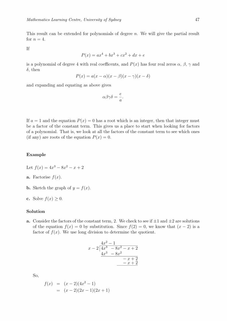
Mathematics Learning Centre, University of Sydney 47
This result can be extended for polynomials of degree n. We will give the partial resultfor n = 4.
If
P (x) = ax4 + bx3 + cx2 + dx + e
is a polynomial of degree 4 with real coefficents, and P (x) has four real zeros α, β, γ andδ, then
P (x) = a(x − α)(x − β)(x − γ)(x − δ)
and expanding and equating as above gives
αβγδ =e
a.
If a = 1 and the equation P (x) = 0 has a root which is an integer, then that integer mustbe a factor of the constant term. This gives us a place to start when looking for factorsof a polynomial. That is, we look at all the factors of the constant term to see which ones(if any) are roots of the equation P (x) = 0.
Example
Let f(x) = 4x3 − 8x2 − x + 2
a. Factorise f(x).
b. Sketch the graph of y = f(x).
c. Solve f(x) ≥ 0.
Solution
a. Consider the factors of the constant term, 2. We check to see if ±1 and ±2 are solutionsof the equation f(x) = 0 by substitution. Since f(2) = 0, we know that (x − 2) is afactor of f(x). We use long division to determine the quotient.
4x2 − 1x − 2 4x3 − 8x2 − x + 2
4x3 − 8x2
− x + 2− x + 2
So,
f(x) = (x − 2)(4x2 − 1)
= (x − 2)(2x − 1)(2x + 1)
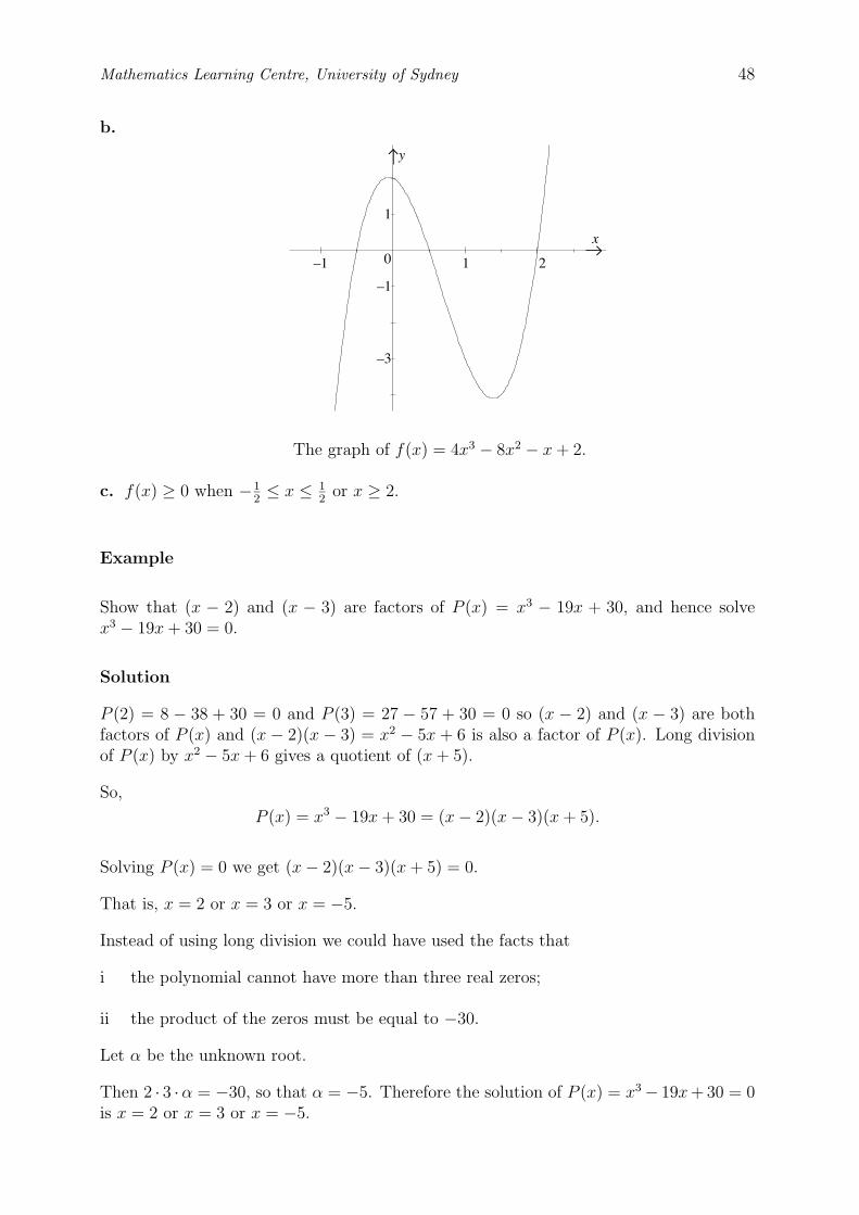
–1 2
x
y
1
1
–1
–3
0
Mathematics Learning Centre, University of Sydney 48
b.
The graph of f(x) = 4x3 − 8x2 − x + 2.
c. f(x) ≥ 0 when −12≤ x ≤ 1
2or x ≥ 2.
Example
Show that (x − 2) and (x − 3) are factors of P (x) = x3 − 19x + 30, and hence solvex3 − 19x + 30 = 0.
Solution
P (2) = 8 − 38 + 30 = 0 and P (3) = 27 − 57 + 30 = 0 so (x − 2) and (x − 3) are bothfactors of P (x) and (x − 2)(x − 3) = x2 − 5x + 6 is also a factor of P (x). Long divisionof P (x) by x2 − 5x + 6 gives a quotient of (x + 5).
So,
P (x) = x3 − 19x + 30 = (x − 2)(x − 3)(x + 5).
Solving P (x) = 0 we get (x − 2)(x − 3)(x + 5) = 0.
That is, x = 2 or x = 3 or x = −5.
Instead of using long division we could have used the facts that
i the polynomial cannot have more than three real zeros;
ii the product of the zeros must be equal to −30.
Let α be the unknown root.
Then 2 · 3 ·α = −30, so that α = −5. Therefore the solution of P (x) = x3 − 19x + 30 = 0is x = 2 or x = 3 or x = −5.
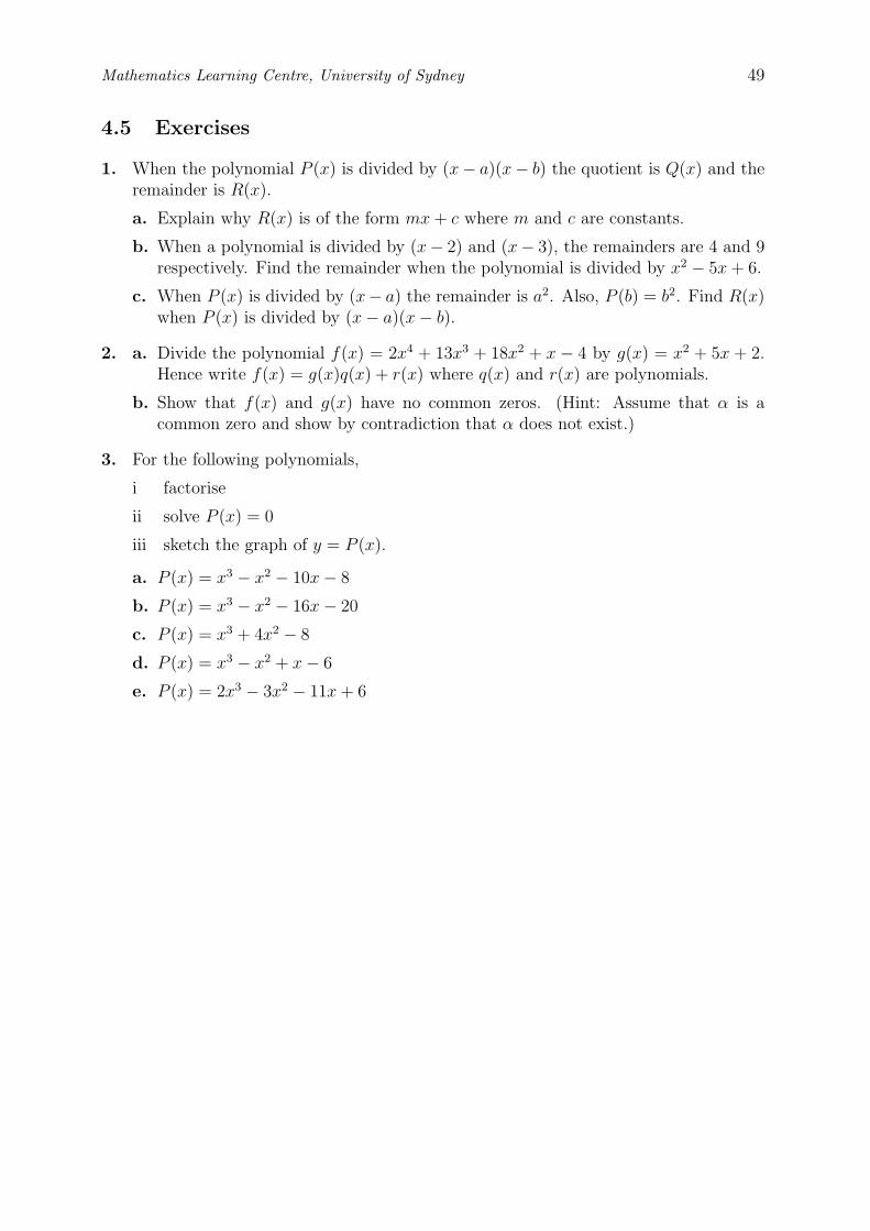
Mathematics Learning Centre, University of Sydney 49
4.5 Exercises
1. When the polynomial P (x) is divided by (x− a)(x− b) the quotient is Q(x) and theremainder is R(x).
a. Explain why R(x) is of the form mx + c where m and c are constants.
b. When a polynomial is divided by (x− 2) and (x− 3), the remainders are 4 and 9respectively. Find the remainder when the polynomial is divided by x2 − 5x + 6.
c. When P (x) is divided by (x− a) the remainder is a2. Also, P (b) = b2. Find R(x)when P (x) is divided by (x − a)(x − b).
2. a. Divide the polynomial f(x) = 2x4 + 13x3 + 18x2 + x − 4 by g(x) = x2 + 5x + 2.Hence write f(x) = g(x)q(x) + r(x) where q(x) and r(x) are polynomials.
b. Show that f(x) and g(x) have no common zeros. (Hint: Assume that α is acommon zero and show by contradiction that α does not exist.)
3. For the following polynomials,
i factorise
ii solve P (x) = 0
iii sketch the graph of y = P (x).
a. P (x) = x3 − x2 − 10x − 8
b. P (x) = x3 − x2 − 16x − 20
c. P (x) = x3 + 4x2 − 8
d. P (x) = x3 − x2 + x − 6
e. P (x) = 2x3 − 3x2 − 11x + 6
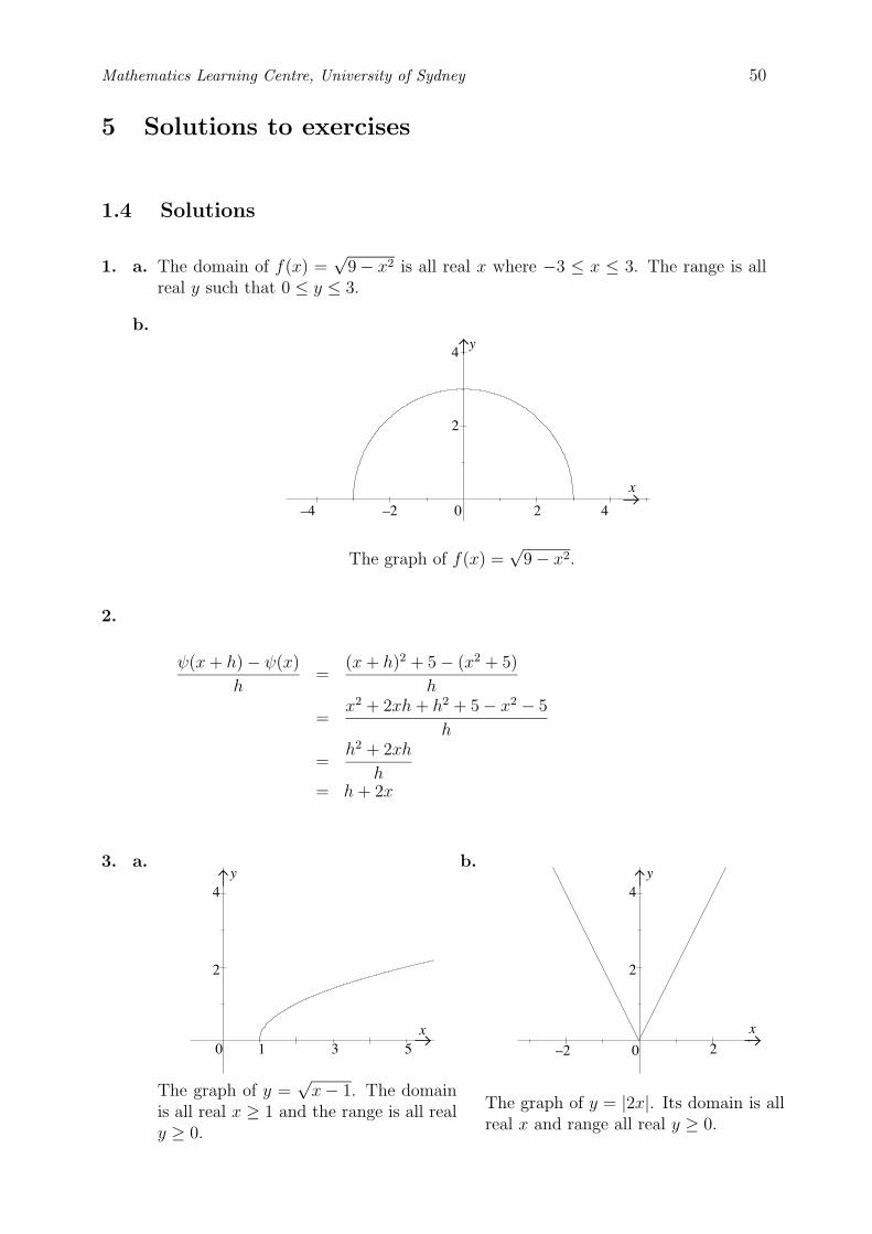
y
0 2 4–2
x
–4
2
4
0
4
x
y
2
1 3 5
4
x
2
y
2
0–2
Mathematics Learning Centre, University of Sydney 50
5 Solutions to exercises
1.4 Solutions
1. a. The domain of f(x) =√
9 − x2 is all real x where −3 ≤ x ≤ 3. The range is allreal y such that 0 ≤ y ≤ 3.
b.
The graph of f(x) =√
9 − x2.
2.
ψ(x + h) − ψ(x)
h=
(x + h)2 + 5 − (x2 + 5)
h
=x2 + 2xh + h2 + 5 − x2 − 5
h
=h2 + 2xh
h= h + 2x
3. a.
The graph of y =√
x − 1. The domainis all real x ≥ 1 and the range is all realy ≥ 0.
b.
The graph of y = |2x|. Its domain is allreal x and range all real y ≥ 0.
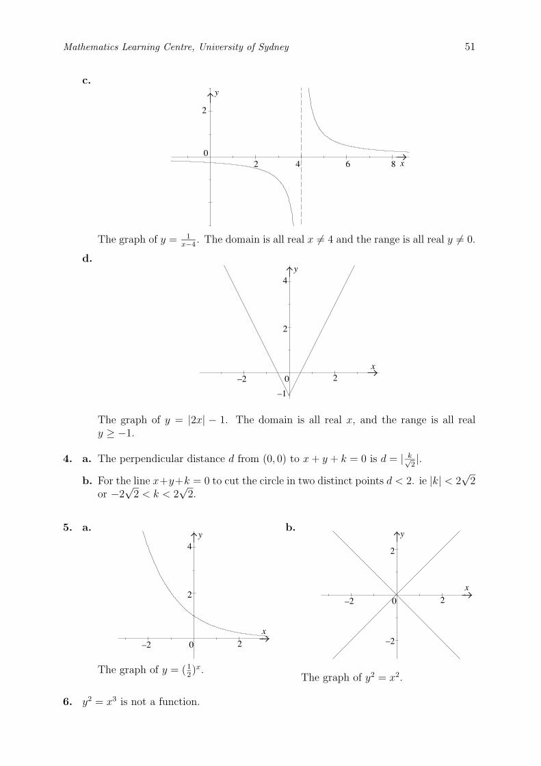
y
0
2
x62 4 8
2
y
2
0–2
4
x
–1
4
x
2
y
2
0–2
2
–2
0–2
x
2
y
Mathematics Learning Centre, University of Sydney 51
c.
The graph of y = 1x−4
. The domain is all real x �= 4 and the range is all real y �= 0.
d.
The graph of y = |2x| − 1. The domain is all real x, and the range is all realy ≥ −1.
4. a. The perpendicular distance d from (0, 0) to x + y + k = 0 is d = | k√2|.
b. For the line x+y+k = 0 to cut the circle in two distinct points d < 2. ie |k| < 2√
2or −2
√2 < k < 2
√2.
5. a.
The graph of y = (12)x.
b.
The graph of y2 = x2.
6. y2 = x3 is not a function.
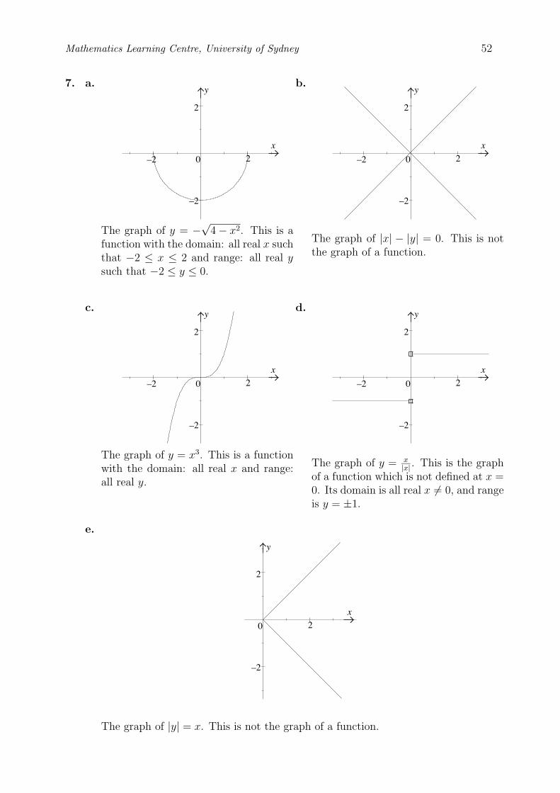
2
–2
0–2
x
2
y
2
–2
0–2
x
2
y
2
–2
0–2
x
2
y
0–2
x
2
y
2
–2
x
2
y
2
–2
0
Mathematics Learning Centre, University of Sydney 52
7. a.
The graph of y = −√
4 − x2. This is afunction with the domain: all real x suchthat −2 ≤ x ≤ 2 and range: all real ysuch that −2 ≤ y ≤ 0.
b.
The graph of |x| − |y| = 0. This is notthe graph of a function.
c.
The graph of y = x3. This is a functionwith the domain: all real x and range:all real y.
d.
The graph of y = x|x| . This is the graph
of a function which is not defined at x =0. Its domain is all real x �= 0, and rangeis y = ±1.
e.
The graph of |y| = x. This is not the graph of a function.
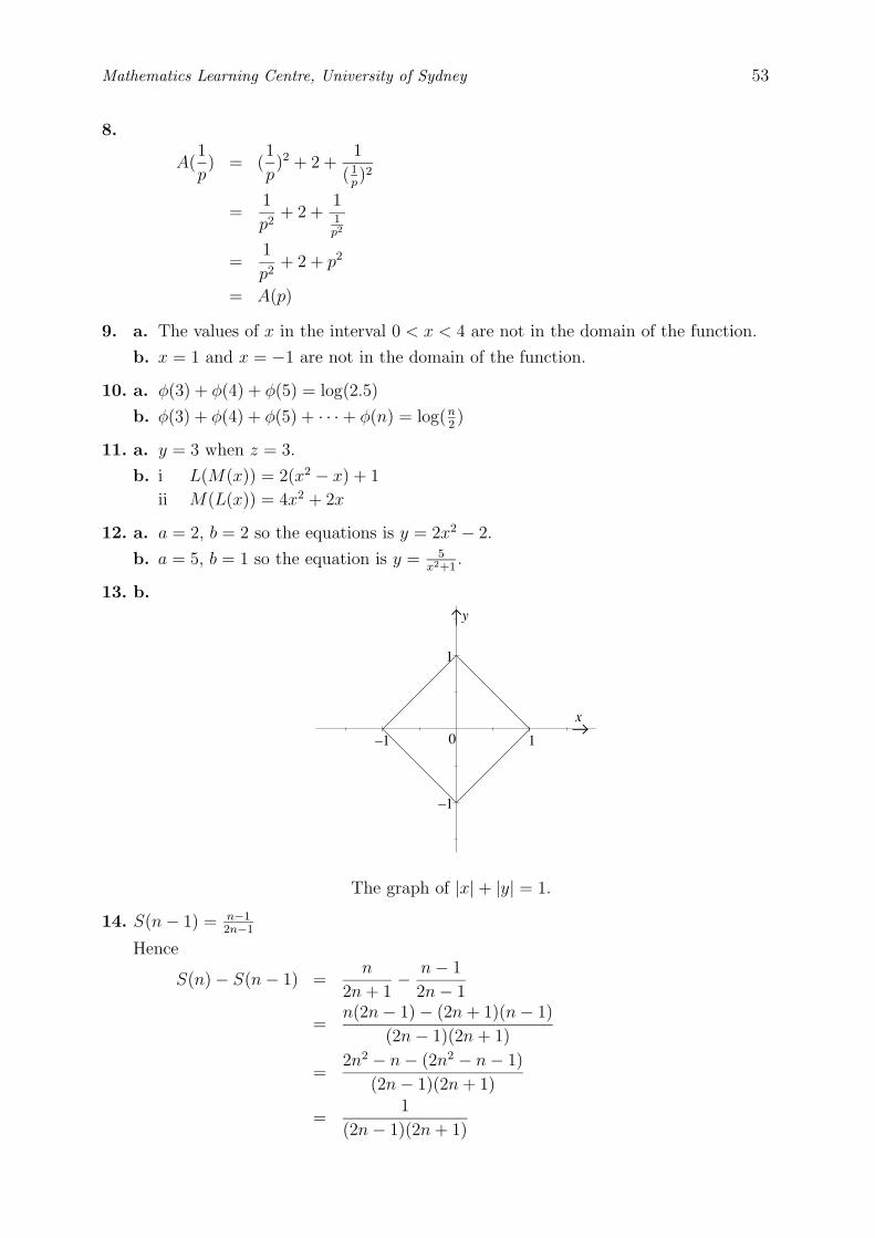
x
1–1
y
1
–1
0
Mathematics Learning Centre, University of Sydney 53
8.
A(1
p) = (
1
p)2 + 2 +
1
(1p)2
=1
p2+ 2 +
11p2
=1
p2+ 2 + p2
= A(p)
9. a. The values of x in the interval 0 < x < 4 are not in the domain of the function.
b. x = 1 and x = −1 are not in the domain of the function.
10. a. φ(3) + φ(4) + φ(5) = log(2.5)
b. φ(3) + φ(4) + φ(5) + · · · + φ(n) = log(n2)
11. a. y = 3 when z = 3.
b. i L(M(x)) = 2(x2 − x) + 1
ii M(L(x)) = 4x2 + 2x
12. a. a = 2, b = 2 so the equations is y = 2x2 − 2.
b. a = 5, b = 1 so the equation is y = 5x2+1
.
13. b.
The graph of |x| + |y| = 1.
14. S(n − 1) = n−12n−1
Hence
S(n) − S(n − 1) =n
2n + 1− n − 1
2n − 1
=n(2n − 1) − (2n + 1)(n − 1)
(2n − 1)(2n + 1)
=2n2 − n − (2n2 − n − 1)
(2n − 1)(2n + 1)
=1
(2n − 1)(2n + 1)
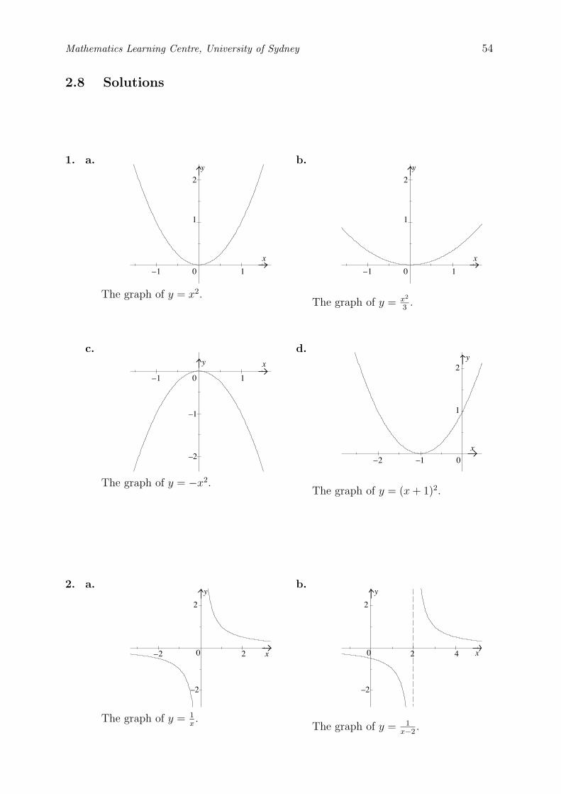
0
1
2
–1
x
y
1
0
1
2
–1
x
y
1
10–1
xy
–1
–2 –1
x
y
1
2
–2 0
2
–2 0
–2
x
y
2
2
0
–2
4 x
y
2
Mathematics Learning Centre, University of Sydney 54
2.8 Solutions
1. a.
The graph of y = x2.
b.
The graph of y = x2
3.
c.
The graph of y = −x2.
d.
The graph of y = (x + 1)2.
2. a.
The graph of y = 1x.
b.
The graph of y = 1x−2
.
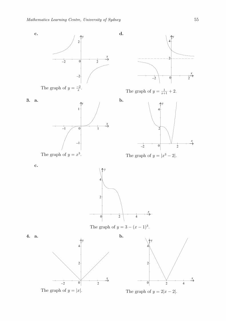
x
y
2
2
0
–2
–2
x
y
2
0 2–2
4
0–1
x
1
y
1
–1x
y
0 2–2
2
4
x
y
40 2
2
4
x
y
0 2–2
2
4
2 4
2
4
x
y
0
Mathematics Learning Centre, University of Sydney 55
c.
The graph of y = −2x
.
d.
The graph of y = 1x+1
+ 2.
3. a.
The graph of y = x3.
b.
The graph of y = |x3 − 2|.
c.
The graph of y = 3 − (x − 1)3.
4. a.
The graph of y = |x|.
b.
The graph of y = 2|x − 2|.
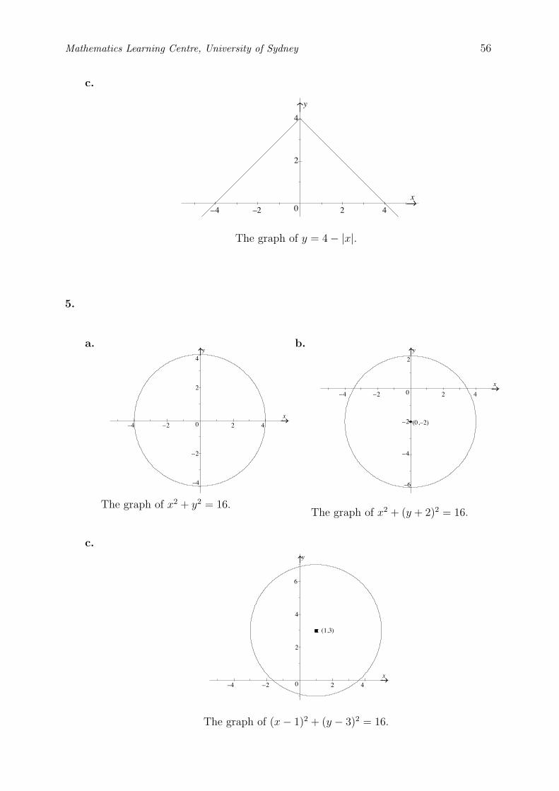
2 4
2
4
x
y
0–2–4
–2–4 2 4
2
4
x
y
0
–2
–4
2 4
x
y
0
2
–6
–2
–4
–2–4
(0,–2)
x
y
0
(1,3)
–2–4 2 4
2
4
6
Mathematics Learning Centre, University of Sydney 56
c.
The graph of y = 4 − |x|.
5.
a.
The graph of x2 + y2 = 16.
b.
The graph of x2 + (y + 2)2 = 16.
c.
The graph of (x − 1)2 + (y − 3)2 = 16.
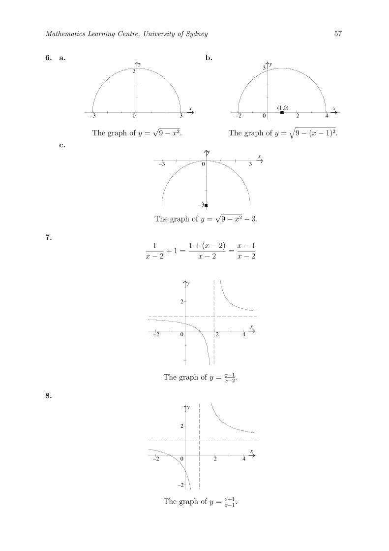
–3 3x
y
0
3
0
3
2 4–2x
y
(1,0)
xy
–3
0–3 3
4–2x
y
0
2
2
4–2x
y
0
2
2
–2
Mathematics Learning Centre, University of Sydney 57
6. a.
The graph of y =√
9 − x2.
b.
The graph of y =√
9 − (x − 1)2.
c.
The graph of y =√
9 − x2 − 3.
7.1
x − 2+ 1 =
1 + (x − 2)
x − 2=
x − 1
x − 2
The graph of y = x−1x−2
.
8.
The graph of y = x+1x−1
.
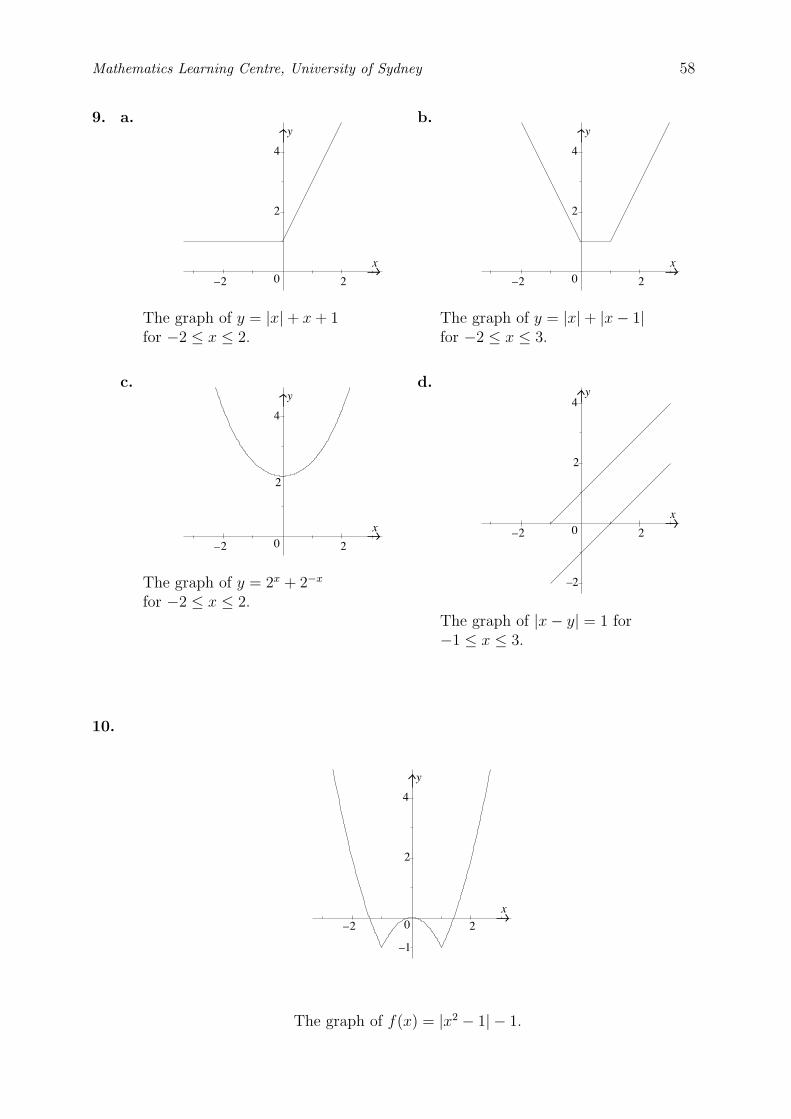
x
y
0 2–2
2
4
x
y
0 2–2
2
4
4
x
y
0 2–2
2
2–2
2
–2
4
x
y
0
2–2
2
–1
4
x
y
0
Mathematics Learning Centre, University of Sydney 58
9. a.
The graph of y = |x| + x + 1for −2 ≤ x ≤ 2.
b.
The graph of y = |x| + |x − 1|for −2 ≤ x ≤ 3.
c.
The graph of y = 2x + 2−x
for −2 ≤ x ≤ 2.
d.
The graph of |x − y| = 1 for−1 ≤ x ≤ 3.
10.
The graph of f(x) = |x2 − 1| − 1.
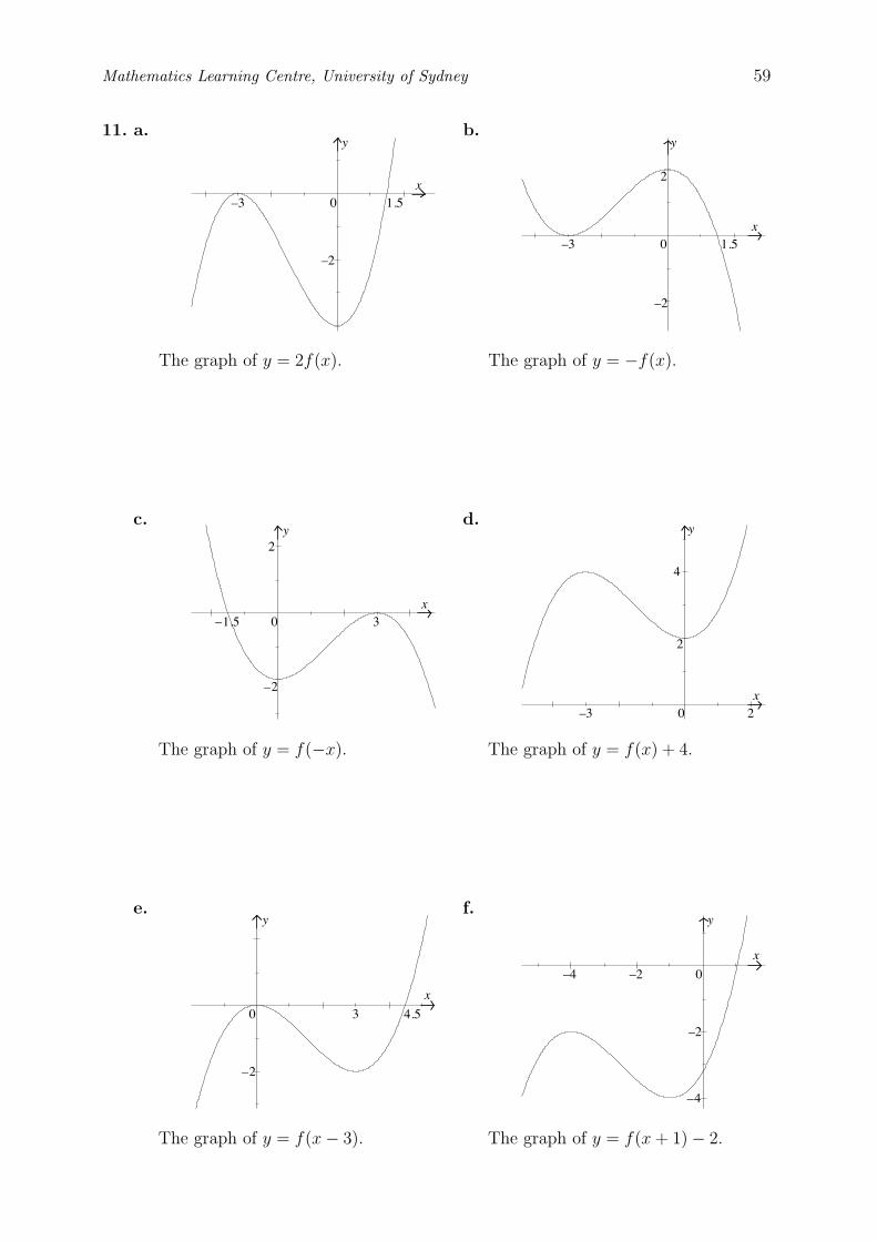
y
0x
–3 1.5
–20
x–3 1.5
2
–2
y
3
–2
y
0x
2
–1.5
x–3
4
2
2
y
0
y
0
x
3 4.5
–2
0
x
–2
–4
–2–4
y
Mathematics Learning Centre, University of Sydney 59
11. a.
The graph of y = 2f(x).
b.
The graph of y = −f(x).
c.
The graph of y = f(−x).
d.
The graph of y = f(x) + 4.
e.
The graph of y = f(x − 3).
f.
The graph of y = f(x + 1) − 2.
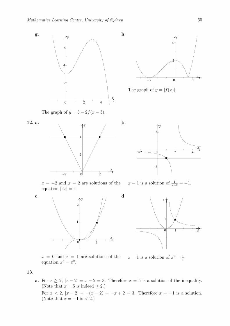
2
2
y
4
6
0 4x
0x
–3 2
2
y
4
2
4
20
x
–2
y
20x
–2 4
–2
y
2
1
2
x
10
y
10
y
1
x
Mathematics Learning Centre, University of Sydney 60
g.
The graph of y = 3 − 2f(x − 3).
h.
The graph of y = |f(x)|.
12. a.
x = −2 and x = 2 are solutions of theequation |2x| = 4.
b.
x = 1 is a solution of 1x−2
= −1.
c.
x = 0 and x = 1 are solutions of theequation x3 = x2.
d.
x = 1 is a solution of x2 = 1x.
13.
a. For x ≥ 2, |x − 2| = x − 2 = 3. Therefore x = 5 is a solution of the inequality.(Note that x = 5 is indeed ≥ 2.)
For x < 2, |x − 2| = −(x − 2) = −x + 2 = 3. Therefore x = −1 is a solution.(Note that x = −1 is < 2.)
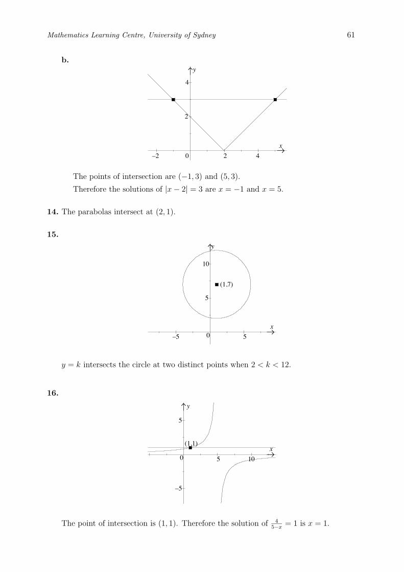
x
2 4–2
2
0
y
4
5
10
5–5
(1,7)
0
y
x
(1,1)
5
50
y
x
10
–5
Mathematics Learning Centre, University of Sydney 61
b.
The points of intersection are (−1, 3) and (5, 3).
Therefore the solutions of |x − 2| = 3 are x = −1 and x = 5.
14. The parabolas intersect at (2, 1).
15.
y = k intersects the circle at two distinct points when 2 < k < 12.
16.
The point of intersection is (1, 1). Therefore the solution of 45−x
= 1 is x = 1.
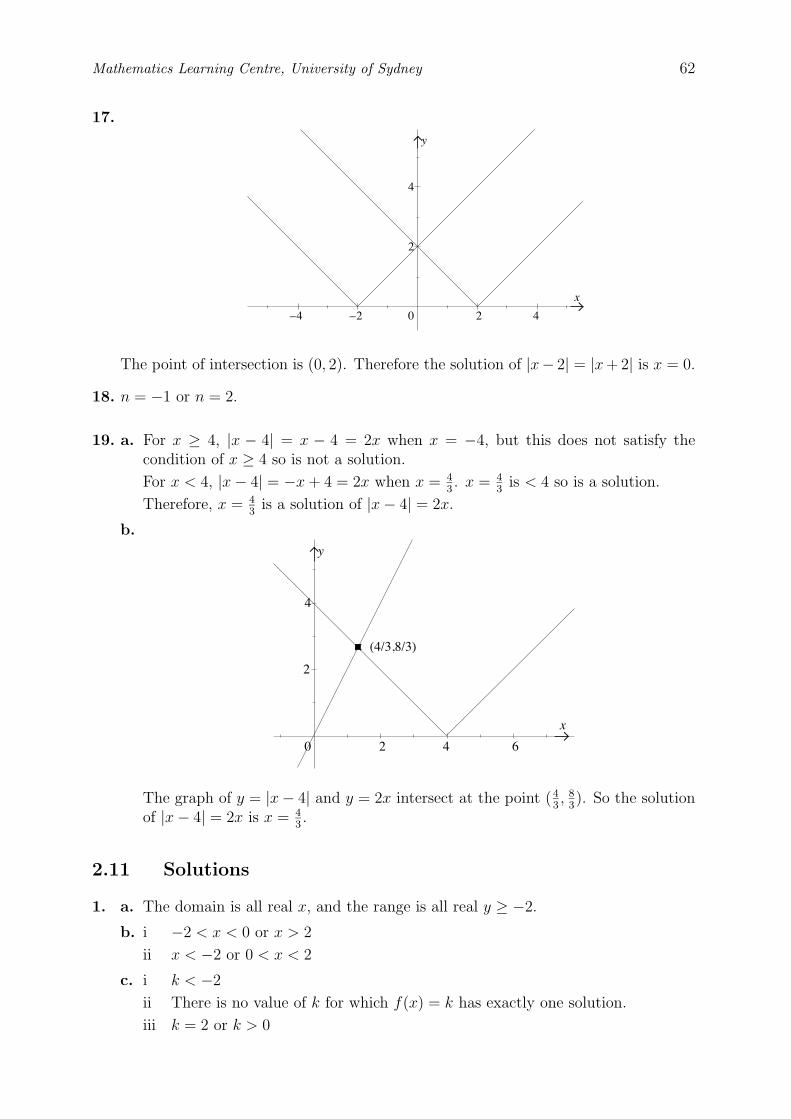
x
2 4–2–4
2
0
y
4
2 4 6
2
0
y
4
x
(4/3,8/3)
Mathematics Learning Centre, University of Sydney 62
17.
The point of intersection is (0, 2). Therefore the solution of |x− 2| = |x + 2| is x = 0.
18. n = −1 or n = 2.
19. a. For x ≥ 4, |x − 4| = x − 4 = 2x when x = −4, but this does not satisfy thecondition of x ≥ 4 so is not a solution.
For x < 4, |x − 4| = −x + 4 = 2x when x = 43. x = 4
3is < 4 so is a solution.
Therefore, x = 43
is a solution of |x − 4| = 2x.
b.
The graph of y = |x − 4| and y = 2x intersect at the point (43, 8
3). So the solution
of |x − 4| = 2x is x = 43.
2.11 Solutions
1. a. The domain is all real x, and the range is all real y ≥ −2.
b. i −2 < x < 0 or x > 2
ii x < −2 or 0 < x < 2
c. i k < −2
ii There is no value of k for which f(x) = k has exactly one solution.
iii k = 2 or k > 0
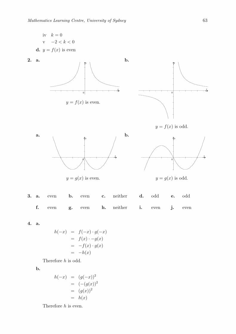
x
y
0
x
y
0
y
0
x
y
0
x
Mathematics Learning Centre, University of Sydney 63
iv k = 0
v −2 < k < 0
d. y = f(x) is even
2. a.
y = f(x) is even.
b.
y = f(x) is odd.
a.
y = g(x) is even.
b.
y = g(x) is odd.
3. a. even b. even c. neither d. odd e. odd
f. even g. even h. neither i. even j. even
4. a.
h(−x) = f(−x) · g(−x)
= f(x) · −g(x)
= −f(x) · g(x)
= −h(x)
Therefore h is odd.
b.
h(−x) = (g(−x))2
= (−(g(x))2
= (g(x))2
= h(x)
Therefore h is even.
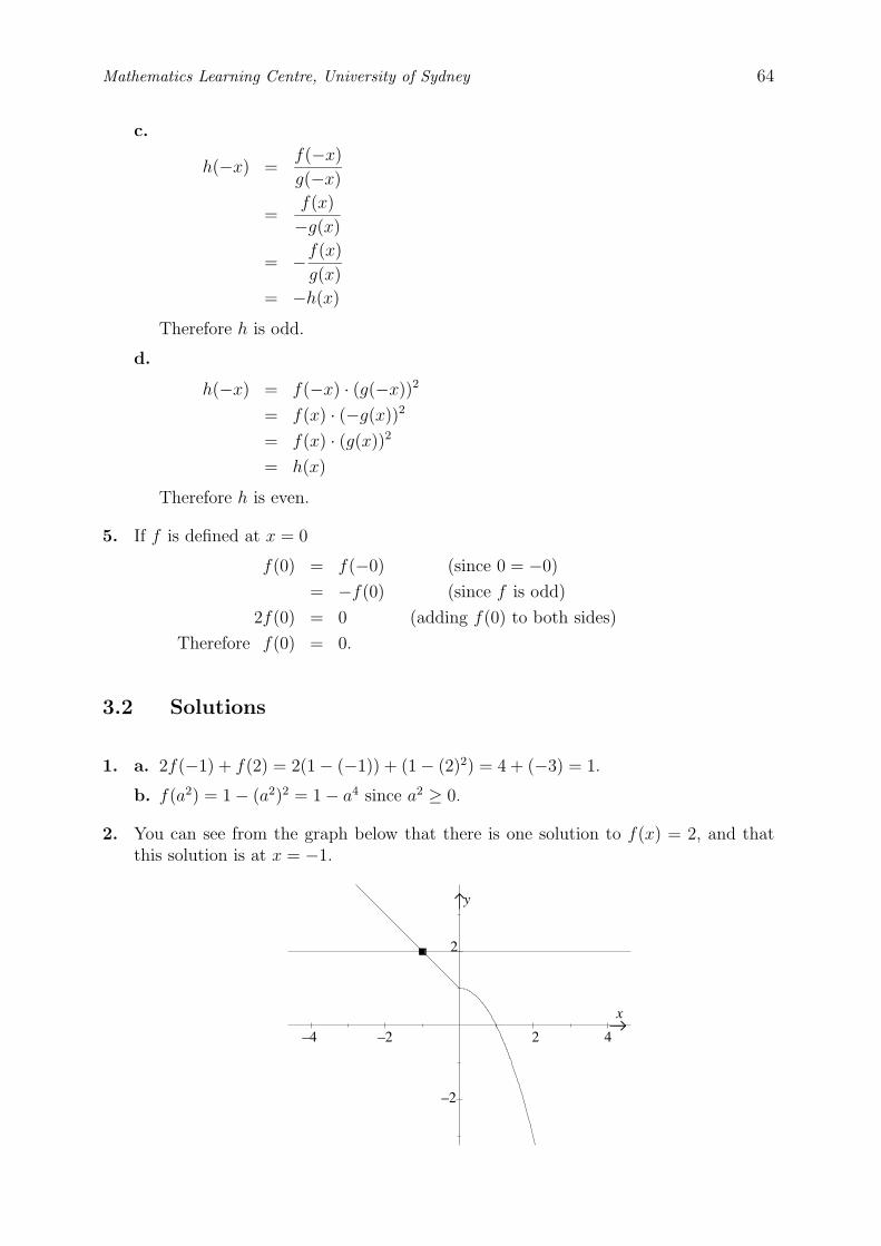
–2
x
y
–4 –2 42
2
Mathematics Learning Centre, University of Sydney 64
c.
h(−x) =f(−x)
g(−x)
=f(x)
−g(x)
= −f(x)
g(x)
= −h(x)
Therefore h is odd.
d.
h(−x) = f(−x) · (g(−x))2
= f(x) · (−g(x))2
= f(x) · (g(x))2
= h(x)
Therefore h is even.
5. If f is defined at x = 0
f(0) = f(−0) (since 0 = −0)
= −f(0) (since f is odd)
2f(0) = 0 (adding f(0) to both sides)
Therefore f(0) = 0.
3.2 Solutions
1. a. 2f(−1) + f(2) = 2(1 − (−1)) + (1 − (2)2) = 4 + (−3) = 1.
b. f(a2) = 1 − (a2)2 = 1 − a4 since a2 ≥ 0.
2. You can see from the graph below that there is one solution to f(x) = 2, and thatthis solution is at x = −1.
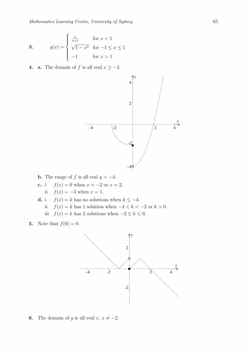
–4 –2 42
4
2
–2
–4
x
y
42
2
–2
–4 –2
x
y
Mathematics Learning Centre, University of Sydney 65
3. g(x) =
1x+1
for x < 1√
1 − x2 for −1 ≤ x ≤ 1
−1 for x > 1
4. a. The domain of f is all real x ≥ −2.
b. The range of f is all real y > −4.
c. i f(x) = 0 when x = −2 or x = 2.
ii f(x) = −3 when x = 1.
d. i f(x) = k has no solutions when k ≤ −4.
ii f(x) = k has 1 solution when −4 < k < −2 or k > 0.
iii f(x) = k has 2 solutions when −2 ≤ k ≤ 0.
5. Note that f(0) = 0.
6. The domain of g is all real x, x �= −2.
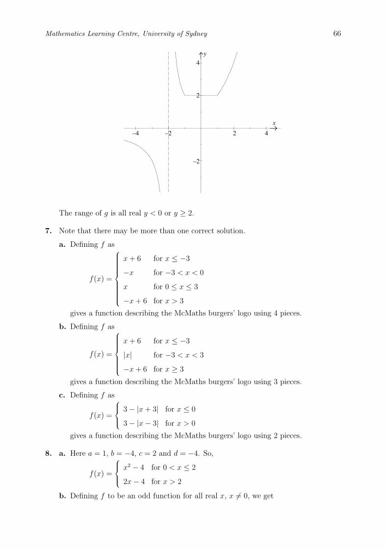
–2
–4 –2
x
4
y
42
2
Mathematics Learning Centre, University of Sydney 66
The range of g is all real y < 0 or y ≥ 2.
7. Note that there may be more than one correct solution.
a. Defining f as
f(x) =
x + 6 for x ≤ −3
−x for −3 < x < 0
x for 0 ≤ x ≤ 3
−x + 6 for x > 3
gives a function describing the McMaths burgers’ logo using 4 pieces.
b. Defining f as
f(x) =
x + 6 for x ≤ −3
|x| for −3 < x < 3
−x + 6 for x ≥ 3
gives a function describing the McMaths burgers’ logo using 3 pieces.
c. Defining f as
f(x) =
3 − |x + 3| for x ≤ 0
3 − |x − 3| for x > 0
gives a function describing the McMaths burgers’ logo using 2 pieces.
8. a. Here a = 1, b = −4, c = 2 and d = −4. So,
f(x) =
x2 − 4 for 0 < x ≤ 2
2x − 4 for x > 2
b. Defining f to be an odd function for all real x, x �= 0, we get
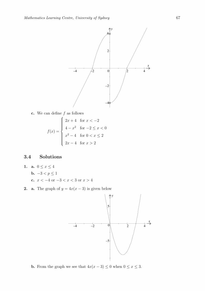
y
42
2
–2
–4 –2
x
0
4
–4
–4 –2
x
5
–5
0
y
42
Mathematics Learning Centre, University of Sydney 67
c. We can define f as follows
f(x) =
2x + 4 for x < −2
4 − x2 for −2 ≤ x < 0
x2 − 4 for 0 < x ≤ 2
2x − 4 for x > 2
3.4 Solutions
1. a. 0 ≤ x ≤ 4
b. −3 < p ≤ 1
c. x < −4 or −3 < x < 3 or x > 4
2. a. The graph of y = 4x(x − 3) is given below
b. From the graph we see that 4x(x − 3) ≤ 0 when 0 ≤ x ≤ 3.
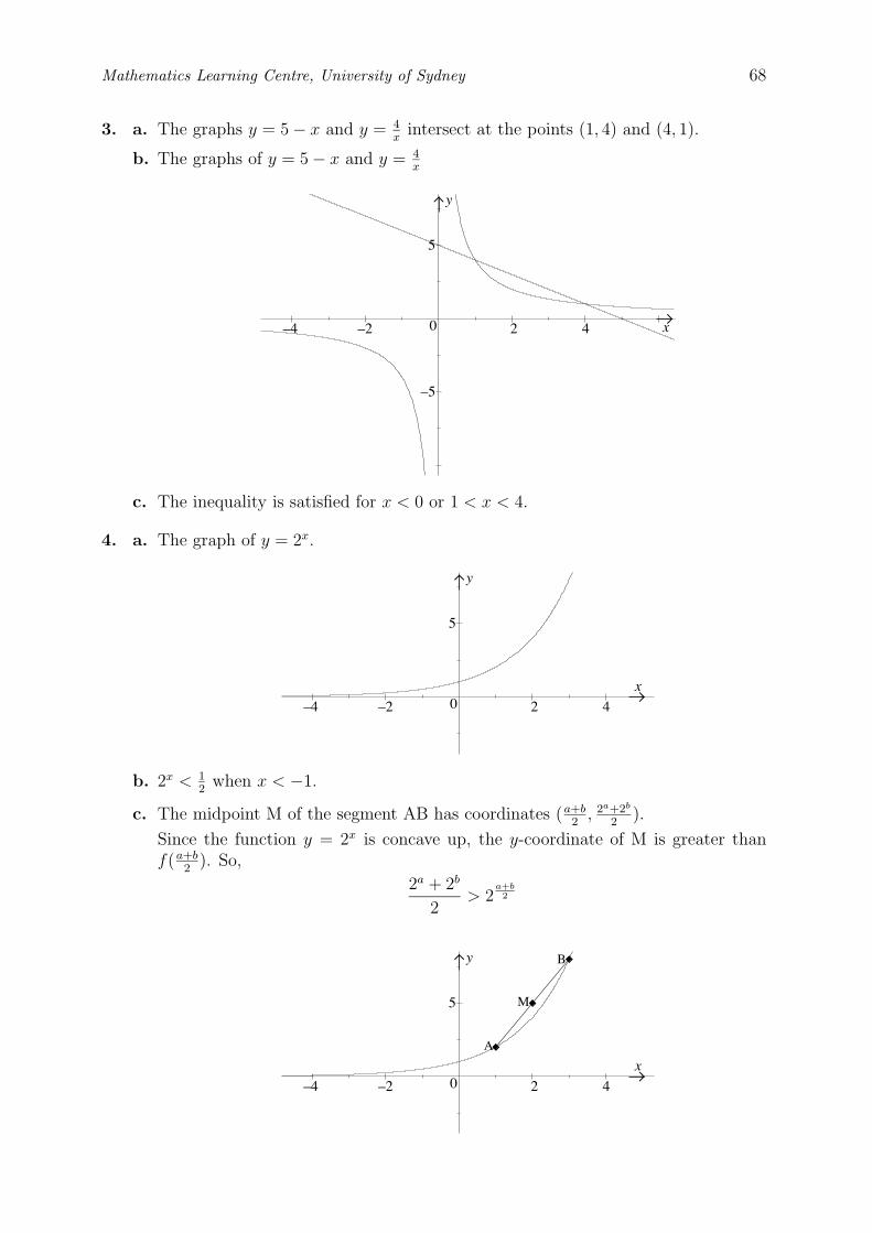
x
5
–5
0
y
42–4 –2
5
0
y
42–4 –2
x
5
0
y
42–4 –2
x
M
A
B
Mathematics Learning Centre, University of Sydney 68
3. a. The graphs y = 5 − x and y = 4x
intersect at the points (1, 4) and (4, 1).
b. The graphs of y = 5 − x and y = 4x
c. The inequality is satisfied for x < 0 or 1 < x < 4.
4. a. The graph of y = 2x.
b. 2x < 12
when x < −1.
c. The midpoint M of the segment AB has coordinates (a+b2
, 2a+2b
2).
Since the function y = 2x is concave up, the y-coordinate of M is greater thanf(a+b
2). So,
2a + 2b
2> 2
a+b2
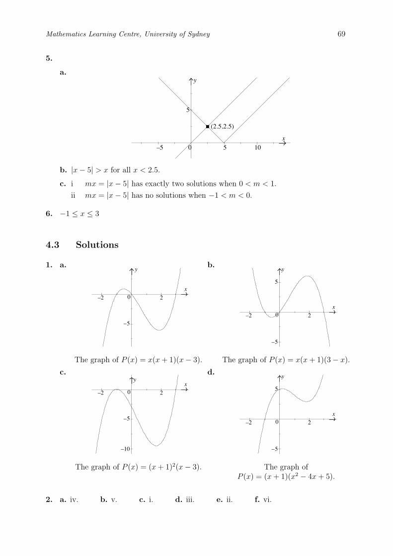
(2.5,2.5)
x
5
0–5
y
5 10
–2
x
y
0 2
–52
–5
–2
x
y
0
5
0 2
–5
–2
xy
–10
2
–5
–2
x
y
0
5
Mathematics Learning Centre, University of Sydney 69
5.
a.
b. |x − 5| > x for all x < 2.5.
c. i mx = |x − 5| has exactly two solutions when 0 < m < 1.
ii mx = |x − 5| has no solutions when −1 < m < 0.
6. −1 ≤ x ≤ 3
4.3 Solutions
1. a.
The graph of P (x) = x(x + 1)(x − 3).
b.
The graph of P (x) = x(x + 1)(3 − x).
c.
The graph of P (x) = (x + 1)2(x − 3).
d.
The graph ofP (x) = (x + 1)(x2 − 4x + 5).
2. a. iv. b. v. c. i. d. iii. e. ii. f. vi.
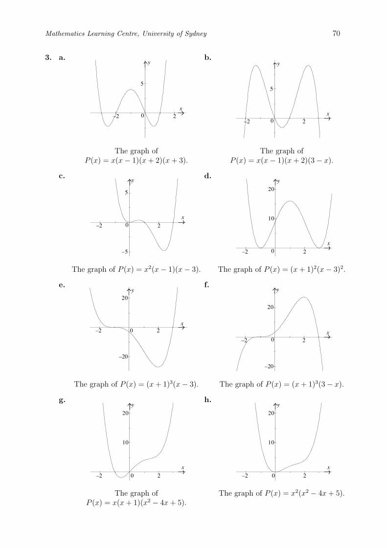
0
5
2–2x
y
5
2–2x
y
0
2
–5
–2
x
y
0
5
0 2–2
x
y
10
20
y
0 2–2x
20
–20
2–2x
20
–20
y
0
2–2
x
y
10
20
0 2–2
x
y
10
20
0
Mathematics Learning Centre, University of Sydney 70
3. a.
The graph ofP (x) = x(x − 1)(x + 2)(x + 3).
b.
The graph ofP (x) = x(x − 1)(x + 2)(3 − x).
c.
The graph of P (x) = x2(x − 1)(x − 3).
d.
The graph of P (x) = (x + 1)2(x − 3)2.
e.
The graph of P (x) = (x + 1)3(x − 3).
f.
The graph of P (x) = (x + 1)3(3 − x).
g.
The graph ofP (x) = x(x + 1)(x2 − 4x + 5).
h.
The graph of P (x) = x2(x2 − 4x + 5).
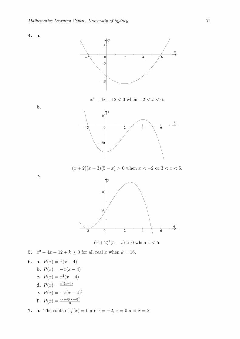
y
42–2
x
–15
5
–5
0 6
42–2
x
0
–20
10
6
y
x
0 6
y
42–2
40
20
Mathematics Learning Centre, University of Sydney 71
4. a.
x2 − 4x − 12 < 0 when −2 < x < 6.
b.
(x + 2)(x − 3)(5 − x) > 0 when x < −2 or 3 < x < 5.
c.
(x + 2)2(5 − x) > 0 when x < 5.
5. x2 − 4x − 12 + k ≥ 0 for all real x when k = 16.
6. a. P (x) = x(x − 4)
b. P (x) = −x(x − 4)
c. P (x) = x2(x − 4)
d. P (x) = x3(x−4)3
e. P (x) = −x(x − 4)2
f. P (x) = (x+4)(x−4)2
8
7. a. The roots of f(x) = 0 are x = −2, x = 0 and x = 2.
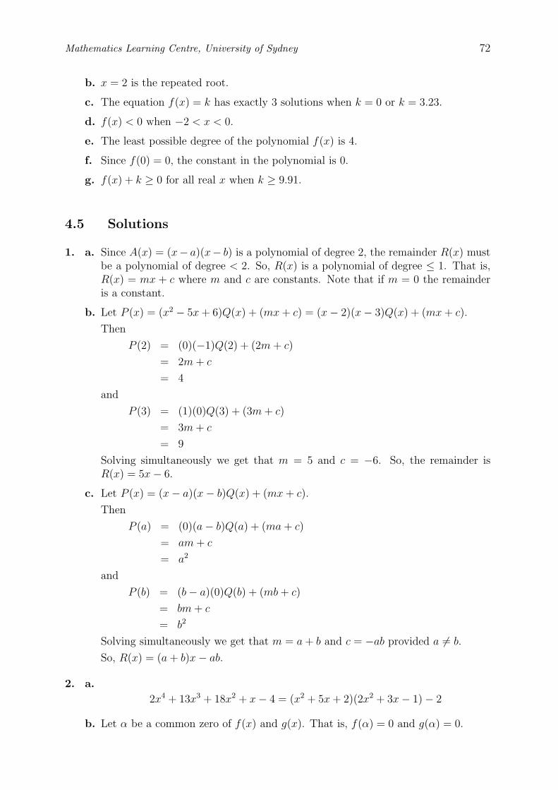
Mathematics Learning Centre, University of Sydney 72
b. x = 2 is the repeated root.
c. The equation f(x) = k has exactly 3 solutions when k = 0 or k = 3.23.
d. f(x) < 0 when −2 < x < 0.
e. The least possible degree of the polynomial f(x) is 4.
f. Since f(0) = 0, the constant in the polynomial is 0.
g. f(x) + k ≥ 0 for all real x when k ≥ 9.91.
4.5 Solutions
1. a. Since A(x) = (x− a)(x− b) is a polynomial of degree 2, the remainder R(x) mustbe a polynomial of degree < 2. So, R(x) is a polynomial of degree ≤ 1. That is,R(x) = mx + c where m and c are constants. Note that if m = 0 the remainderis a constant.
b. Let P (x) = (x2 − 5x + 6)Q(x) + (mx + c) = (x − 2)(x − 3)Q(x) + (mx + c).
Then
P (2) = (0)(−1)Q(2) + (2m + c)
= 2m + c
= 4
and
P (3) = (1)(0)Q(3) + (3m + c)
= 3m + c
= 9
Solving simultaneously we get that m = 5 and c = −6. So, the remainder isR(x) = 5x − 6.
c. Let P (x) = (x − a)(x − b)Q(x) + (mx + c).
Then
P (a) = (0)(a − b)Q(a) + (ma + c)
= am + c
= a2
and
P (b) = (b − a)(0)Q(b) + (mb + c)
= bm + c
= b2
Solving simultaneously we get that m = a + b and c = −ab provided a �= b.
So, R(x) = (a + b)x − ab.
2. a.
2x4 + 13x3 + 18x2 + x − 4 = (x2 + 5x + 2)(2x2 + 3x − 1) − 2
b. Let α be a common zero of f(x) and g(x). That is, f(α) = 0 and g(α) = 0.
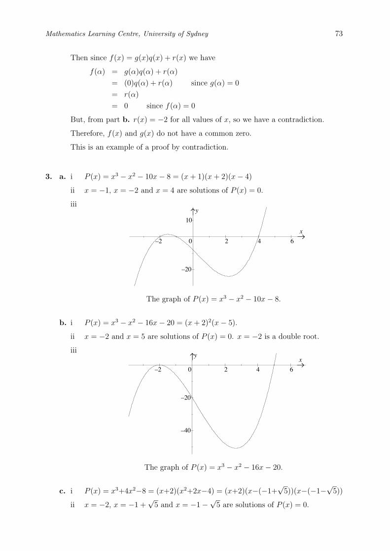
2–2
x
10
–20
0 6
y
4
0 6
y
42–2
x
–20
–40
Mathematics Learning Centre, University of Sydney 73
Then since f(x) = g(x)q(x) + r(x) we have
f(α) = g(α)q(α) + r(α)
= (0)q(α) + r(α) since g(α) = 0
= r(α)
= 0 since f(α) = 0
But, from part b. r(x) = −2 for all values of x, so we have a contradiction.
Therefore, f(x) and g(x) do not have a common zero.
This is an example of a proof by contradiction.
3. a. i P (x) = x3 − x2 − 10x − 8 = (x + 1)(x + 2)(x − 4)
ii x = −1, x = −2 and x = 4 are solutions of P (x) = 0.
iii
The graph of P (x) = x3 − x2 − 10x − 8.
b. i P (x) = x3 − x2 − 16x − 20 = (x + 2)2(x − 5).
ii x = −2 and x = 5 are solutions of P (x) = 0. x = −2 is a double root.
iii
The graph of P (x) = x3 − x2 − 16x − 20.
c. i P (x) = x3+4x2−8 = (x+2)(x2+2x−4) = (x+2)(x−(−1+√
5))(x−(−1−√
5))
ii x = −2, x = −1 +√
5 and x = −1 −√
5 are solutions of P (x) = 0.
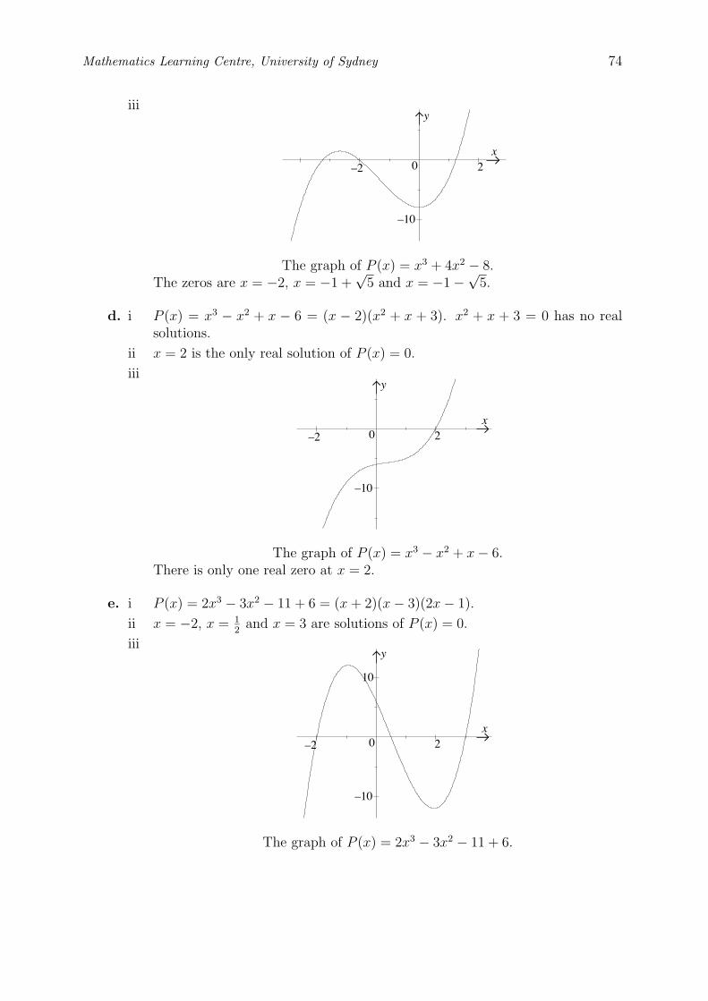
y
–10
0 2–2
x
–2
x
y
–10
0 2
–10
0 2–2
x
y
10
Mathematics Learning Centre, University of Sydney 74
iii
The graph of P (x) = x3 + 4x2 − 8.The zeros are x = −2, x = −1 +
√5 and x = −1 −
√5.
d. i P (x) = x3 − x2 + x − 6 = (x − 2)(x2 + x + 3). x2 + x + 3 = 0 has no realsolutions.
ii x = 2 is the only real solution of P (x) = 0.
iii
The graph of P (x) = x3 − x2 + x − 6.There is only one real zero at x = 2.
e. i P (x) = 2x3 − 3x2 − 11 + 6 = (x + 2)(x − 3)(2x − 1).
ii x = −2, x = 12
and x = 3 are solutions of P (x) = 0.
iii
The graph of P (x) = 2x3 − 3x2 − 11 + 6.
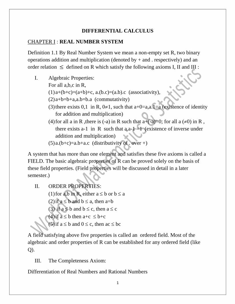
1
DIFFERENTIAL CALCULUS
CHAPTER I : REAL NUMBER SYSTEM
Definition 1.1 By Real Number System we mean a non-empty set R, two binary
operations addition and multiplication (denoted by + and . respectively) and an
order relation defined on R which satisfy the following axioms I, II and III :
I. Algebraic Properties:
For all a,b,c in R,
(1) a+(b+c)=(a+b)+c, a.(b.c)=(a.b).c (associativity),
(2) a+b=b+a,a.b=b.a (commutativity)
(3) there exists 0,1 in R, 01, such that a+0=a,a.1=a (existence of identity
for addition and multiplication)
(4) for all a in R ,there is (-a) in R such that a+(-a)=0; for all a (0) in R ,
there exists a-1 in R such that a.a-1 =1 (existence of inverse under
addition and multiplication)
(5) a.(b+c)=a.b+a.c (distributivity of . over +)
A system that has more than one element and satisfies these five axioms is called a
FIELD. The basic algebraic properties of R can be proved solely on the basis of
these field properties. (Field properties will be discussed in detail in a later
semester.)
II. ORDER PROPERTIES:
(1) for a,b in R, either a b or b a
(2) if a b and b a, then a=b
(3) if a b and b c, then a c
(4) if a b then a+c b+c
(5) if a b and 0 c, then ac bc
A field satisfying above five properties is called an ordered field. Most of the
algebraic and order properties of R can be established for any ordered field (like
Q).
III. The Completeness Axiom:
Differentiation of Real Numbers and Rational Numbers
2
Let . If a real number M satisfies for all , then is called
an upper bound of and is called bounded above.
If a real number satisfies (1) is an upper bound of and (2) no real number
less than is an upper bound of , then is the LEAST UPPER BOUND of or
SUPREMUM of , written as l.u.b. or sup .
Ex: sup {
+ = 0 , sup { } does not exist, sup
{1,2,3}=max{1,2,3}.
The Completeness Axiom for R states that:
Every nonempty subset S of R that is bounded above has a least upper bound in R.
That is, if a nonempty subset of real numbers has an upper bound, then it has a
smallest upper bound in R.
Definition: A number is called an algebraic number if it satisfies a polynomial
equation
where the coefficients ,
, ………… , , are integers, , and . A real number which is not
algebraic (like ) is called a transcendental number.
Note: Rational numbers are algebraic numbers since a rational number
,
are integers and satisfies the equation .
Theorem: Suppose that , , ………… , are integers and is a rational
number satisfying the polynomial equation
where , and . Write
, where are integers
having no common factors and . Then divides and divides .
Ex: √ cannot represent a rational number.
»By theorem above, the only rational numbers that could possibly be solutions of
are and . But none of the four numbers and are
solutions of the equation. Since √ represents a solution of , √
cannot represent a rational number. Note: In , division of an integer
by an integer is defined iff there exists unique integer such that holds.
3
For , division of by is undefined because there does not exist any
integer such that holds. Division of by is undefined because for
any integer holds and uniqueness of is violated.
The absolute value function and the greatest integer function
For , absolute value of , denoted as | |, is defined to be the distance
between (the points representing) and :
| | , if ,
, if .
The absolute value function satisfies the following properties:
(1) | | | |, (2) | | | | | |, (3) | |
| || |,
(4) |
|
| |
| |( ) (5) || | | || | |
Note: | | gives distance between the (points representing) real numbers and
. Hence the statement lies between and can be equivalently put as
| | .
The greatest integer function is defined on the set of real numbers as follows:
for real number a satisfying , ( an integer), , - .
Thus, for example, , - , for ,
, for
, for
CHAPTER 2: SEQUENCES OF REAL NUMBERS
4
Definition: A sequence (in ) is a function ( ) is called the n th term
of the sequence and denoted by . The sequence is often denoted by
* , + or ,more compactly, by ( ). We must distinguish between a
sequence ( ) and its range set * +: the range set of (1,1/2,1/3,…) is
{1,1/2,1/3,…}; that of (1,1,1…) is {1}. We shall use the terms
‘bounded’,’unbounded’, ‘bounded above’ and ‘bounded below’ for a sequence iff
its range set (as a subset of ) has the corresponding property. ( ) is bounded,
( ) is bounded below but not above, ( ) is bounded above but not below,
(( ) ) is neither bounded above nor bounded below.
Note: A fraction increases when either the numerator is increased and/or the
denominator is decreased.
Ex: Verify whether the following sequences are bounded above and/or bounded
below: (1) .
/, (2)
.( )
/, (3) ( ) where √
√
, (4)
( ) where
√
√ .
Solution: (1)
4
5
( )
, for all natural
number . Thus
, for all natural ; hence .
/ is bounded.
(2) |( )
|
for all natural : hence .( )
/ is
bounded.
(3)
( ) ( )
for all (justify!): hence ( ) is bounded.
(4)
√
√
for all natural : hence ( ) is bounded.
Definition: A sequence ( ) is convergent iff there exists such that for
every , there exists natural number ( ) , in general depending on , so that
implies | | . In this case, we say ( ) converges to as
or is a limit of ( ) and write ( ) . A sequence that is
not convergent is called divergent.
5
Ex: Consider the sequence ( ), where for all . Then
( ) , since for any , | | for all .
Note that every constant sequence (b,b,…) is convergent to b.
Ex: Consider the sequence ( ), where ( ) natural .
( ) since the open interval (0.5 , 1.5) containing 1 does not contain all
the infinite number of terms of the sequence with odd suffix . ( ) since
the open interval (-1.5 ,-0.5) containing -1 does not contain all the infinite number
of terms of the sequence with even suffix.
If let *| | | |+. Then ( , ) does not
contain any term of the sequence. Hence ( )diverges.
Ex: If
for all natural ,
then ( ) : for any , | |
0
1
Note: Observe the direction of implication sign carefully.
Note: If ( ) then the inequality || | | || | |, natural,
shows that | | | |. Converse may not hold as can be seen from the
counter example (( ) ).
Theorem: A convergent sequence is bounded.
»Let ( ) . Corresponding to , there exists positive integer
such that | | that is for all
. Let * + and
* +. Then for all natural . Hence
( ) is bounded.
Theorem: (Limit Theorem for Sequences) Let ( ) and
( ) .

6
Then (1) ( ) , (2)
( ) , (3)
( ) , (4) if , then ∃
such that for all and .
/
.
Note: Combined applications of different parts ensures that ( )
and ( ) if .
Note: Note that it is possible that ( ) and ( ) , , for all
natural and yet . Consider the sequences ( ) ( ) where and
for all .
Theorem: If ( ) and ( ) are convergent sequences of real numbers and if
for all ( fixed natural number), then ( ) ( ) .
Theorem: (Sandwich Theorem) Let ( ) ( ) ( ) be sequences and be
such that for all and ( ) ( ) . Then
( ) .
Ex: Let | | . Then ( ) .
» If , the result is obvious. Let . Let
| | . Then and
| | ( ) for all natural . Hence | |
. Since
(
) , by Sandwich Thorem, (| | ) . Hence ( )
Ex: Let . Then (
) .
» If , nothing remains to prove.
Let . Then
for all natural .
Let
for natural . then ( ) ( )
,
so that for all .
By Sandwich Theorem, ( ) , so that , (
) .
7
If , let so that (
) .
/ , since and
hence (
) .
Ex: (
) .
»Since (
) for all , we can write
where for all .
Hence ( )
( )
( )
.
Thus √
. Thus ( ) and so (
) .
E x a m p l e 2 . 1 1 Let
, for natural . clearly
for all natural , where ∑
and
∑
. Since ( ) ( ) , so ( ) .
Ex: Use Squeeze Theorem to verify whether following sequences converge:
.
/ .( )
/.
»
, 1 ( )
( )
for all natural .
Note: Every convergent sequence is bounded. The converse may not hold :
consider (( ) ). We now consider a class of sequences for which convergence is
equivalent to boundedness.
Definition: A sequence or ( ) is monotonically increasing iff is
monotonically increasing function, that is, for all natural . A sequence
or ( ) is monotonically decreasing iff is monotonically decreasing
function, that is, for all natural . A sequence is monotonic iff it is
either monotonically increasing or monotonically decreasing.
Theorem : A monotonically increasing sequence is convergent iff it is bounded
above.
8
Ex: Consider ( ), where
for natural . ( ) is
monotonially increasing. Also
.
/ for all natural . Thus ( ) is convergent.
Ex: Consider ( ), where .
/
.
Now, .
( )
( )( )
(
)
(
) (
) (
)
.
Thus , for all .
Hence ( ) is bounded.
Also
.
/
.
/ .
/ .
/
( ) .
/ .
/ .
/ .
/.
Thus is sum of ( ) summands whereas an is that of ( ) summands
and each summand (from beginning) of is greater than or equal to the
corresponding summand of . Hence ( ) is monotone increasing. Thus ( ) is
convergent. If we denote ( ) by , then since for all
.
Ex: Consider the sequence ( ), where
, for all . Clearly
( ) is monotonically increasing. For each ,
.
/
.
/
.Hence there is no such
that , for all . Thus ( ) is unbounded above and hence is not
convergent.
9
Ex: Consider the sequence ( ), where
. Clearly (an) is
monotonically increasing. Also, for each ,
( )
.
/ .
/
. So ( ) is bounded above. Hence
( ) is convergent.
Ex: Consider the sequence ( ), where
for each . clearly
( ) is monotonically increasing. We have seen in two examples above that
( ) is divergent if and convergent if . This implies that ( ) is
divergent if and convergent if , because for each
if
while
if .
P R O P E R L Y D I V E R G E N T S E Q U E N C E S
Definition: Let ( ) be a sequence of real numbers. ( ) tends to as tends to
written as ( ) iff for every , there exists natural number
such that implies . Similarly, a sequence ( ) of real numbers
tends to as tends to , written as ( ) iff for every ,
there exists natural number such that implies .
CAUCHY’S GENERAL PRINCIPLE OF CONVERGENCE
Theorem: A sequence ( ) of real numbers is convergent iff for every ,
there exists positive integer such that for natural number,
| | holds.
Ex: Verify that the sequence ( ) where
natural, does not
converge.
»If ( ) converges, then corresponding to
, there exists such that
| |
for all . In particular, | |
. But | |
, contradiction.
10
Definition: An infinite series, or, for short, a series of real numbers is an
expression of the form or, in more compact notation
∑ , where is real number , for all . The sequence ( ), where
, is called the sequence of partial sums corresponding to the series
∑ .
Definition: We say ∑ is convergent iff ( ) exists as real number, that
is, iff the sequence of partial sums of the series is convergent. If ( )
, then is the sum of the series ∑ and we write ∑
. An infinite
series ∑ that is not convergent, is divergent. In particular, we say the series
∑ diverges to or to according as ( ) or ( )
.
Note: The convergence of a series is not affected by changing finite number of its
terms, although its sum may change by doing so. If ∑ and
∑ be two series obtained by changing first m number of terms, and
if ( ) and ( ) be the corresponding sequences of partial sums, then for
∑ ∑
. Thus ( )converges iff ( )converges and if
they converge to and respectively, ∑ ∑
.
Ex: (Geometric Series) For the series ∑ ( real ),
, if and
, if .
If , ( )
. Hence the series ∑ converges for
.
If , then for all (since are ); hence ( )
and thus ∑ diverges to .
CHAPTER 3: INFINITE SERIES OF REAL NUMBER
11
If , and for all n and hence ∑ is divergent.
Finally, if , then ( ) and ( ) ; hence ∑
is divergent to
Ex: (Exponential Series) We have seen earlier that the sequence ( ) given by
is convergent to a real number . Thus
…….
Ex: (Harmonic series and its variants) As seen in example 2.17,
is divergent for and convergent for . It can be shown that the
sequence of partial sums and hence the series ∑( )
converges.
Note: Since convergence of a series is defined in terms of convergence of its
sequence of partial sums, many results about convergence of a series follows from
the corresponding results on sequences.
The sequence of partial sums of a convergent series is bounded.
Let ∑ , ∑ . Then ∑( ) , ∑( ) . If
for all , then .
(Sandwich Theorem) If ( ) ( ) ( ) are sequences of real numbers such
that for each , and further if ∑ ∑ , then
∑ .
Theorem: If ∑ is convergent, then ( ) . In other words, if ( )
does not exist or is not equal to zero, then ∑ is divergent. Converse may not
hold: consider ∑
.
Ex: ∑ ( )
is divergent if since |( )
| for all .
TESTS FOR CONVERGENCE : series of non-negative terms
Theorem: (Comparison Test) Let ( ) ( ) be sequences of non-negative real
numbers such that for all natural. If ∑ is convergent, then
∑ is convergent and ∑ ∑ . If ∑ diverges, then ∑ is divergent.
12
Ex: ∑
is convergent since
.
/ for all natural and ∑.
/ is
convergent.
Ex: ∑
( )
is convergent since
( )
for all natural and ∑
is
convergent.
Theorem: (Limit Form of Comparison Test) Let ( ) ( ) be sequences of
positive real numbers such that .
/ ( ). Then ∑ is
convergent iff ∑ is convergent. If .
/ and if ∑ is convergent,
then ∑ is convergent. If .
/ and if ∑ is divergent, then ∑ is
divergent.
Ex: The series ∑
is convergent by Comparison Test since ∑.
/ is
convergent and .
/ ( ).
Ex: ∑ .
/ diverges by comparison test since ∑
is divergent and
.
/
( )
Theorem: (D’Alembert’s Ratio Test) Let ∑ be a series of positive real numbers
and let .
/ . Then ∑ converges if and ∑ diverges if
.
Theorem: (Cauchy’s Root Test) Let ∑ be a series of positive real numbers and
let
. Then ∑ converges if and ∑ diverges if .
Theorem: (Raabe’s Test) Let ∑ be a series of positive real numbers and let
.
/ .Then ∑ converges if and ∑ diverges if
.
13
Ex: Use comparison Test to verify whether the following series converge:
(1) ∑
, (2) ∑
√ ( )(3)∑
√
( )
»Compare the series respectively with (1) ∑
, (2)∑
and
(3)∑
Note: While testing convergence of a series ∑ by comparison test, the series is
constructed by considering heighest power of n present in numerator and
denominator separately .
ALTERNATING SERIES : LEIBNITZ TEST
Definition: A series of the form ∑( ) , where for all positive integer
, is an alternating series.
Theorem: (Leibnitz Test) An alternating series ∑( ) is convergent if the
sequence ( )of positive terms is monotonically decreasing and ( ) .
Ex: 1 4 ∑( )
converges by Leibnitz Test.
Definition: Let and .
A real number is the LEFT( hand) LIMIT of at , written as ,
iff for every , there exists such that implies | ( )
| .
CHAPTER 4
LIMIT OF A REAL VALUED FUNCTION OF A REAL VARIABLE
14
A real number is the RIGHT( hand) LIMIT of at , written as ,
iff for every , there exists such that implies | ( )
| .
A real number is limit of at , written as , iff
(1) exists and (2) exists and (3) .
Ex: Prove that .
»Let be given.| | | |
| | ,
. Hence the result.
Note: Observe the direction of implication sign carefully.
Ex:
=0
»Let be given. |
| | | |
| | | | |
| | √ | | .
Ex: Let ( ) , -.
since for any , there exists such that
implies | ( ) |=| | . Similarly,
. Hence does not exist.
Ex: Let ( )
( ) .
As ,
and so
.
As ,
and so
So
does not exist while
.
Theorem: (Sequential criteria of limits) Let and be a real number.
Then the following are equivalent:
15
(1) ,
(2) for every sequence ( ) of real numbers that converges to such that
for all , the sequence ( ( )) converges to .
Theorem: (Divergence criteria) Let and be a real number.
iff there exists a sequence ( ) of real numbers that converges to
such that for all , ( ) but ( ( )) (either ( ( ))
does not exist or exists but not equal to ).
Alternatively, does not exist iff there exist sequences ( ) and ( ) of
real numbers, , for all , ( ) ( ) , but
( ( )) ( ( )) .
Ex: .
/ does not exist in .
» The sequences ( ) and ( ) both converge to where
and
( )
but ( .
/) ( ) tends to whereas ( ( )) ( (
)
) converges to .
Theorem: (Limit Theorem of Functions) Let and . If
and , then ( ) , (
) , ( ) , ( ) . If Let
( ) for all real belonging to ( ), for some , and if
, then (
)
.
Note: If be a polynomial, then ( ) for any real .
Theorem: (Squeeze Theorem) Let and . If ( ) ( )
( ) for all real , and if , then .
Some Extensions of Limit Concept
Definition: Let Let and . tends to as , written as
, iff for every real , there exists such that for all
satisfying | | , ( ) holds.
16
Definition: Let and . tends to as , written as
, iff for every real , there exists such that for all
satisfying | | , ( ) holds.
Ex:
.
»Let
√
√ | |
√ .
Hence the result.
Definition: Let . A real number is a limit of as , written as
, iff for any given , there exists such that implies
| ( ) |
Definition: Let . tends to as tends to , written as ,
iff given any real , there exists such that implies ( ) .
E x a m p l e 4 . 8 Evaluate the following limits or show that they do not exist:
(1)
, (2)
√ , (3)
√
√ ( ) (4)
√
√
( )
»(1)Let
( ).
Hence
.
(2) Let
√
√ √
.
Hence
√ .
(3) Let √
√ |
√
√ |
√
√
.
Hence √
√ .
17
Continuous Functions
Definition: Let and let be a real number. is continuous at iff
, and ( ) exists and ( ) If
is continuous at every real is continuous on .
Theorem: Let be continuous at and be a real constant.
Then the functions are continuous at , where the
functions are defined as follows:
( )( ) ( ) ( )
( )( ) ( ) ( )
( )( ) ( ) ( )
( )( ) ( ) .
The function
defined by .
/ ( )
( )
( ) is continuous at if ( ) for all
in ( ) for some .
Ex: Every constant function ( ) ( real constant) is continuous
on .
Ex: Every polynomial function ( )
is
continuous on .
Definition: has removable discontinuity at iff
exists but either ( ) does not exist or exists but
different from the limiting value .
has discontinuity of first kind at iff both and
exist but .
has discontinuity of second kind at iff at least one of and
does not exist.
Ex: Check the continuity of the following functions at the indicated points:
(1) ( ) , - , - , (2) ( )
,
18
(3) ( )
(4) ( ) , - ( ) ( )
( )
» (1) = ( )=-1= ( ( ))=
( ).
Hence has removable discontinuity at .
(2)
(
) ,
(
)
Thus ( ) Hence is continuous at .
(3)
.
/ ;
( ) and
( ) . Hence is continuous at .
(4) ( ) ( ) ; hence
has discontinuity of first kind at .
(5) does not exist as real number; hence has discontinuity of
second kind at .
Theorem: If be continuous at and be continuous at ( )
then ,defined by ( )( ) ( ( )) for real , is continuous at .
Ex: ( ) and ( ) are continuous on ;
hence ( )( ) ( ) is continuous on .
Theorem: If is continuous at and ( ) , then there exists such
that ( ) has the same sign as ( ) for all in ( )
Theorem: (Bolano’s Intermediate Value Property) Let be continuous
and be real numbers, , such that ( ) ( ). Let be a real
number between ( ) and ( ) Then there exists in , - such that
( )
Note: Continuity is sufficient but not necessary for the conclusion in the above
theorem to hold: for example, let us define
19
( )
, satisfies IVP but is discontinuous at
Corollary: If f(a) and f(b) are of opposite signs, then there exists c in (a,b) such
that f(c)=0.
Ex: Prove that
has a solution between 1 and 2.
»Let f( ) ( )( ) ( )( ) ( )( ) being a
polynomial function, is continuous at any real number and hence on , -. Also
( ) and ( ) . Thus there exists in ( ) such that ( ) , that is
has a solution in ( )
Ex: Show that the equation has solution in (
)
»Let ( ) ,
- ( ) and (
) ; also is continuous
on ,
- Hence there exists in (
) such that ( ) is a solution of the
given equation.
Theorem: Let be continuous and be real numbers, . Then
there exist in , - such that ( ) * ( ) , -+ and
( ) * ( ) , -+
Note: The result may not hold if we consider a discontinuous function or a non-
closed interval.
Let ( )
for
at .
So is discontinuous at . There does not exist in , - such that
( ) * ( ) , -+ ( ) ( ) does not have either
maximum or minimum on ( )
20
CHAPTER 5
DERIVATIVE OF A REAL VALUED FUNCTION OF A REAL
VARIABLE
Definition: Let , - The left (hand) derivative of at ,
denoted by ( )( ) is equal to ( ) ( )
, provided the limit exists. The
right(hand) derivativeof at , denoted by ( )( ), is equal to ( ) ( )
,
provided the limit exists.
Ex: Let ( ) real constant. is derivable at iff ( )( )
exists and in that case ( )( ) ( ) ( )
In general,
derivative of a constant function defined on an interval at any point of its domain
of definition is zero.
Ex: Let , - ( )
at
for
( )( ) ( ) ( )
( )
while
( )( ) ( ) ( )
. Since ( )( )
( )( ) , is not derivable at . Since ( )( )
( ) ( )
( ) , so is differentiable at and
( )( ) .
Theorem: If , - be differentiable at , then is continuous
at .
, ( ) ( )- 0 ( ) ( )
( )1
( ) ( )
( )
( )( ) . Hence
( ) ( ) thus
is continuous at .
21
Note: Converse may not hold: Consider , - ( ) | | is
continuous at but not differentiable at
Ex: Let ( ) ( ) ( ) for all real . Let ( ) and ( )( )
prove that ( )( ) .
( ) ( ) ( ) ( ) ; hence ( ) . Now ( )( )
( ) ( )
( ) ( ) ( )
( ) ( )
( )( ) .
Definition: Let , - is (monotonically) increasing on , - iff
, - imply ( ) ( ) is (monotonically) decreasing on , - iff
, - imply ( ) ( ) is monotonic iff is either
increasing on , - or decreasing on , - is strictly increasing iff
, - imply ( ) ( ) Similarly strictly decreasing function is
defined.
Theorem: Let , - be a differentiable function. Then
(1) is nonnegative throughout , - iff is monotonically increasing on , -
(2) is positive throughout , - implies is strictly increasing on , -
Ex: Prove that ( )
( are constants) is either
monotonically increasing on or monotonically decreasing on .
( )( )
( ) for all if and for all if
22
CHAPTER 6
SUCCESIVE DIFFERENTIATION
Definition: Let , - be differentiable on , - Then ( ) , - is a
function . This function ( ) may again be differentiable at every point of , -
the function ( ( ))( ) is denoted by ( )and called second order derivative of ,
( ), in its turn, may have derivative at every point of , -, which is denoted by
( ) , called third order derivative of . The process may be continued.
Ex: Let rational. Show that ( ) ( ) (
) , for natural
» ( ) . Result holds for . Let ( ) ( ) (
) , for some natural . Then ( ) ( ( ))( ) ( ) (
)( ) . Thus if the result holds for , it holds for . Thus , by
mathematical induction , the result holds for all natural .
Ex: Let
. Then ( )
( )
( ) .
Ex: Let . Then ( ) . Hence ( ) ( ( ))( ) ( )( ) ( ) ( )
.
Ex: Let . To prove: ( ) (
) ( natural).
( ) (
) Result holds for . Let ( ) (
) for
some natural . Then ( ) .
/ .
/
(( )
). Hence the result holds by induction.
Ex: Let
Then ( ) ( )
Let .
23
Then √ and satisfies and .
Thus ( ) ( )
Hence ( ) ( ) ( ) ( )
Ex: Let
( )( )
. Equating coefficients of like powers
of in the identity ( ) ( ) we get
. Hence
(
) Thus ( )
( )
0
( )
( ) 1.
Ex: Let
( )( )
»
. Thus ( ) -
( )
( ) . Hence ( )( )
Theorem: ( Leibnitz’s Theorem) Let be two functions possessing th order
derivatives, then is differentiable times and
( )( ) .
/ ( ) .
/ ( ) ( ) .
/ ( ) ( ) .
/ ( )
Proof: ( )( ) ( ) ( ) ( ) ( ) (
) ( ) Thus the result holds for
Let ( )( ) ( ) ( ) (
) ( ) ( ) (
) ( ) ( )
( ) ( )
Then ( )( ) (( )( ))( )
0.
/ ( ) .
/ ( ) ( ) .
/ ( ) ( ) .
/ ( )1
( )
,.
/ ( ) .
/ ( ) ( )- ,.
/ ( ) ( ) .
/ ( ) ( )-
,.
/ ( ) ( ) .
/ ( )-
( ) ( ) (
) ( ) ( ) (
) ( ) ( )
(
) ( )
24
since ( ) (
) (
) ) holds. Thus result holds by mathematical
induction.
Ex: Let ( )
Prove that (1) ( ) ( ) ( ) ,
(2) ( ) ( ) ( ) ( ) ( ) ( )
» ( ) ( ) .
√ .
Squaring and cross multiplying, ( )( ( )) ( )
( ) (from given expression).
Hence ( ) ( )( ) ( ( )) ( ) ( )).
Since for the given expression ( ) is not identically zero and the relation is to hold
for all , cancelling ( ) from both sides, we obtain ( ) ( ) ( )
.
Next applying Leibnitz’s Theorem (remembering that th order derivative of sum
and difference of a finite number of functions is sum or difference of their th
order derivatives), we get
,( )( ( ))( ) ( )( ( ))( )( ) (
)( ( ))( )( )]
, ( ( ))( ) ( )( ( ))( ) ( ) ; simplifying we obtain the result.
CHAPTER 7
MEAN VALUE THEOREMS
Theorem: (Rolle’s Theorem) If , - is continuous on , - and
differentiable on ( ) and if ( ) ( ) then there is ( ) such that
( ) .
Ex: If ( ) for , where and , then has a
unique real root. To see this, note that if had more than one real root, then there
would be with and ( ) ( ) . Hence , by Rolle’s Theorem,
there would be ( ) such that ( ) . But ( ) is not zero
25
for any since . On the other hand, and
.Thus takes on negative as well as positive values. Hence ( ) for some
, since has the IVP on . Thus has a unique real root.
Ex: Consider f:[0,1] R defined by f(x)=x, x [0,1) and f(1)=0. Then f is
differentiable on (0,1) and f(0)=f(1)=0 but f is not continuous on [0,1]. Note that
f (c)=1 0 for 0<c<1.
Ex: Consider f:[-1,1] R defined by f(x)=|x|. Then f is continuous on [-1,1] and f(-
1)=f(1)=1. f '(x)=1 for x>0, =-1, for x<0 and f '(0) does not exist. There does not
exist c, -1<c<1, such that f '(0)=0.
Ex: Consider f:[0,1] R defined by f(x)=x for x [0,1). Then f is continuous on
[0,1]and differentiable on (0,1) but f '(c)=1 0 for every c (0,1). Note that f(0)
f(1).
Theorem: (Lagrange’s Mean Value Theorem) If f:[a,b] R is continuous on [a,b]
and differentiable on (a,b), then there exists c (a,b) such that f(b)-f(a)=(b-a)f
'(c).
Proof: Consider F:[a,b] R defined by F(x)=f(x)-f(a)-s(x-a), where s = ( ) ( )
.
Then F(a)=0 and by our choice of constant s, F(b)=0. So Rolle’s Theorem applies
to F and, as a result, there exists c (a,b) such that F/(c)=0, that is, f '(c)=s, as
desired.
Note: If we write b=a+h, then the conclusion of MVT may be stated as follows:
f(a+h)=f(a)+hf '(a+h) for some (0,1).
Corollary: (Mean Value Inequality) If f:[a,b] R is continuous on [a,b] and
differentiable on (a,b),and if m,MR are such that m f '(x) M for all x (a,b),
then m(b-a) f(b)-f(a) M(b-a).
Corollary: Let I be an interval containing more than one point and f: I R be any
function. Then f is a constant function on I if and only if f/ exists and is identically
zero on I.
26
Proof: If is a constant function on , then it is obvious that exists on and
( ) for all .
Conversely, if exists and vanishes identically on , then for any x1 , x2 I with
x1 < x2, we have [x1 , x2] I and applying MVT to on [x1 , x2], we obtain [f(x2)-
f(x1)]=(x2 – x1)f/(c ) (for some ( ) ) and hence ( ) ( ).
Note: The MVT or the Mean Value Inequality may be used to approximate a
differentiable function around a point. For example, if m is natural and ( ) √
for , - then √ √ ( ) ( ) ( )
√ for
some ( ) Hence
√ √ √
√ . For example,
by putting ,
√ √
.
Corollary: Let I be an interval containing more than one point and f: I R be a
differentiable function. Then (1) f ' is nonnegative throughout I iff f is
monotonically increasing on I, (2) f ' is positive throughout I implies f is strictly
increasing .
Proof: Let x1 , x2 I with x1 < x2 . Then [x1 , x2] I and we can apply MVT to
the restriction of to [x1 , x2] to obtain [f(x2)-f(x1)]=(x2 – x1)f '(c ) for some
( ) . Thus f(x2) f(x1) iff f '(c ) .
Note: ( ) is strictly increasing on , - but ( ) .
Theorem: (Cauchy’s MVT) Let f,g: [a,b] R are continuous on [a,b] and
differentiable on (a,b), then there is c (a,b) such that
g(1)
(c)(f(b)-f(a))= f(1)
(c)(g(b)-g(a))
Proof: Consider the function F:[a,b] R defined by F(x)= f(x)-f(a) - s[g(x)-g(a)],
where s = ( ) ( )
( ) ( ).
Theorem: (L’Hospital’s Rule for
Indeterminate Form) Let and (
) be differentiable function such that and .
27
Suppose ( )( ) for all ( ) and ( )( )
( )( )=L. Then
( )
( ) .
Here can be a real number or .
Note: L’Hospital’s Rule for
Indeterminate Form is also valid for right (hand)
limits. The statement is similar to that given above. Combining the two cases
follows L’Hospital’s Rule for(two-sided)limits of
Indeterminate Form, which we
may state as follows:
Theorem: Let and ( ) ( ) for some . Let
be differentiable functions such that and .
Suppose ( )( ) for all and ( )( )
( )( ) . Then
( )
( ) .
Here can be a real number or .
L’Hospital’s Rule for
Indeterminate Form are also valid if instead of considering
limits as , where is a real number, we consider limits as or as
For example, a statement for limits as would be as follows:
Theorem: Let be real number and ( ) be differentiable functions
such that and . Suppose ( )( ) for all in
( ) and ( )( )
( )( ) . Then
( )
( ) . Here can be a real
number or or .
Theorem: (L’Hospital’s Rule for
Indeterminate Form) Let be an interval , )
where is real and either is real with or Let be
differentiable functions such that | ( )| . Suppose ( )( ) for
all and ( )( )
( )( ) Then
( )
( ) Here can be a real
number or or .
28
Theorem: (Taylor’s Theorem) Let be a nonnegative integer and , - be
such that ( ) ( ) ( ) exist on , - and further ( ) is continuous on
, - and differentiable on ( ). Then there exists ( ) such that
( ) ( ) ( ) ( )( ) ( ) ( )( )
( )
( )( )
( )
Proof: For , - let ( ) ( ) ( )( )( ) ( )( )
( )
( )( )
( ) Consider , - defined by ( ) ( ) ( )
( ) , where ( ) ( )
( ) . Then ( ) and our choice of is such that
( ) . So Rolle’s Theorem is applicable to on , - and, as a result, there is
( ) such that |( ) . Next , ( )( ) ( )( ) and so ( )( ) as
well. Now Rolle’s Theorem applies to the restriction of ( ) to , -, and so there
is ( ) such that ( )( ) . Further , if , then ( )( ) and so
there exists ( ) such that ( )( ) . Continuing this way, we see that
there is ( ) such that ( )( ) . Now ( ) is identically
zero, since is a polynomial of degree n. In particular, ( )( ) Hence
( )( ) ( ) which, in turn, yields desired result.
Note: (1)Note that the Lagrange’s MVT corresponds to the case n=0 of Taylor’s
Theorem.
(2) In statement of Taylor’s Theorem , the point was the left end point of
the interval on which was defined. There is an analogous version for right
endpoint: if is as in the statement of Taylor’s Theorem, then there exists
( ) such that ( ) ( ) ( )( )( ) ( )( )
( )
( )( )
( ) ( ) Similarly, it can be proved that if is any interval, ,and
is such that ( ) ( ) ( ) exist on and ( )exists at every
interior point of , then for any , there is between and such that
( ) ( ) ( )( )( ) ( )( )
( )
( )( )
( ) (
) .
29
The last expression is sometimes referred to as the Taylor formula for
around . The polynomial given by ( ) ( ) ( )( )( ) ( )( )
( ) is called the th Taylor polynomial of around .The
difference ( ) ( )( )
( ) ( ) is called Lagrange form
of remainder after terms.
(3) Usually, the Taylor polynomial of around provides a
progressively better approximation to around as increases. For
example, let us revisit the estimate of √ obtained from Lagrange’s MVT and
see what happens when we use Taylor’s Theorem.
Thus let be natural and , - ( ) √ . Applying Taylor
formula for around , with , we have ( ) ( ) ( )( )(
) ( )( )
( ) for some between and .
In particular, for , we get √ √
√
√ for some
( )
For example, by putting , we obtain
√
√
and hence
√
√ , where in the last inequality we have used
the estimate √ . The resulting bounds and are, in fact,
better than the bounds and obtained using MVT.
Taylor’s Infinite Series: Let f be a function possessing derivatives of all orders in
, - for some . The th Taylor Polynomial around for different
positive integers are given by
( ) ( ) ( )( ) ( ) ,
( ) ( ) ( )( )
( )( ) ( )
( )( )
30
( ) ( ) ( )( )
( )( )
( )( ) ( )
( )( )
( )( ) ,
( ) ( ) ( )( )
( )( )
( ) ( )( )
( )(
) ( ) ( )( )
( )( )
( ) ( )( ) where
are in general different real numbers lying strictly between 0 and 1.
Let us denote ( ) ( )( )
( )( )
( ) ( )( ) by . Thus
( ) , where ( ) is the sequence of partial sums corresponding the
infinite series of real numbers
( ) ( )( )
( )( )
( ) ( )( ) If ( ) ,
then ( ) ( ) and we can write
( ) ( ) ( )( )
( )( )
( ) ( )( )
Note: Let be a function possessing derivatives of all orders in , - for some
and let (
( )( )) . Then the Taylor’s infinite series
corresponding to about is :
( ) ( ) ( )( )
( )( )
( ) ( )( ) is called
Maclaurin’s infinite series.
Ex: (The Exponential Series) ( ) , possesses derivatives of every
order in , - for an arbitrarily fixedx and
( )( ) as
since .
/ is bounded for all positive integer (since
implies ). Thus can be expanded in Maclaurin’s
infinite series and
31
Ex: (The sine and cosine series) Let ( ) , then ( )( ) .
/
for all natural number Thus possesses derivatives of all orders in , - Also
.
/ as since .
/ and | .
/| for all . Thus can be expanded in Maclaurin’s infinite series
CHAPTER 8
FUNCTIONS OF SEVERAL REAL VARIABLES
Let be a real-valuedfunction of two independent real variables: we shall
often write ( ) where are independent real variables and is the
dependent real variable. Just as we represent function of a single real variable by a
planar curve in two-dimensional plane, similarly a real-valued function of two
independent real variables is represented by a surface in the three-dimensional
space.
Definition: Let and ( ) . A real number is limit of as
( ) ( ), written as ( ) ( ) , if and only if for every ,
there exists such that √( ) ( ) implies | ( )
| .
( ) ( )
.
»Let be given.
|
| | || | |
| | || | (since |
| for real
)
| | √ | | √ (since , )
√( ) ( ) (say). Hence the result.
32
Definition: Let and ( ) . f is continuous at ( ) iff
( ) ( ) ( )
is continuous at ( ) iff for any two sequences ( ) and ( ) ,
the sequence ( ) should converge to ( )
Ex: Let , ( )
for ( ) ( ) and ( ) .
( ) ( ) does not exist since for sequences .
/ and .
/ (both of which tend
to as ), .
/=
as ; whereas for the sequences .
/ and
.
/(both of which tend to as ), .
/=
as . Hence
is not continuous at ( )
Definition: Let and ( ) . The partial derivative of with respect
to first independent variable at ( ) denoted by ( ) is defined by
( ) ( )
, provided the limit exists. Similarly the partial derivative of
with respect to second independent variable at ( ) denoted by ( ), is
defined by ( ) ( )
, provided the limit exists.
Ex: Find ( ) and ( ) for ( )
, if they exist.
» ( )
( )
.
Definition: The partial derivatives ( ) and ( )of the function ( ) are ,
in turn, functions of and . Thus, if the associated limits exist, we may define
partial derivatives of higher order for s follows :
( ) ( ) ( )
,
( ) ( ) ( )
, ( )
( ) ( )
33
( ) ( ) ( )
.
Here
,
,
,
,
,
.
Ex: If ( ) prove that
(1)
, (2)
( )
» ( )( )( )
Thus ( ) ( ) ( ) where is
an imaginary cube roots of unity. Now
,
,
.
Thus
, since . Similarly the other part
cn be proved .
Homogeneous functions : Euler’s Theorem
Definition: is homogeneous of degree iff ( ) ( ) for all
and for every positive
( )
is homogeneous of degree ( ) is not
homogeneous.
Theorem: (Euler’s Theorem for two independent variables) If is a homogeneous
function of degree having continuous partial derivatives, then
Ex: If
, prove that
(1)
,
34
(2)
( ) .
» is not homogeneous but
is homogeneous of degree 2 and
partial derivatives
and
exist and are continuous at all points except at
( ) hence we can apply Euler’s Theorem on at all points other than ( ) We
get
; or,
or,
.
Differentiating partially w.r.t. and respectively,
,
. Multiplying the equations by
and respectively and adding,
( ) .
/
( )
( ) .
Ex: If .
/ .
/ and have continuous partial derivatives, prove that
.
» .
/ and .
/ are homogeneous functions of degree 1 and 0 respectively and
the functions have continuous partial derivatives; hence , .
/-
, .
/-
.
/
and , .
/-
, .
/-
. From first relation, .
/ ( ) .
/ (( ) )
( ) .
/ .
/ .
/, ( ) .
/ .
/ ( ) .
/ .
/ . Differentiating the
relations w.r.t and respectively and multiplying by and and adding , we
obtain required relation.
35
Definition: Let possess partial derivatives at ( ) is
differentiable at ( ) iff for all and ( ) ( )
( ) ( ) ( ) ( ) where ( ) ( ) ( )
( ) ( ) ( ). ( ) ( ) ( ) is called total
differential of .
CHAPTER 9
APPLICATIONS OF DIFFERENTIAL CALCULUS
TANGENTS AND NORMALS TO A PLANE CURVE
Equation of the tangent to a curve in Cartesian form
The equation of tangent to a planar curve whose equation is given in Cartesian
explicit form ( ) at a point ( ) on the curve is given by:
|( )
( )
The equation of normal to ( ) at a point ( ) (that is, a line through
( ) perpendicular to the tangent at ) is given by:
|( )
( )
(In both cases, we assume that the line is not parallel to the y-axis; otherwise, the
equation is .)
If the equation of the curve is in the implicit form ( ) , we calculate
.
If the equation of the curve is in the parametric form ( ) ( ) then
.
Let T and G be the points of intersection of the tangent PT drawn at P with the x-
axis and N be the foot of the perpendicular from P on the x-axis. Then subtangent
at P is
and subnormal at P is
(NT and NG are the signed
36
distance from N to T and G and may be positive or negative). Length of the tangent
PT is the absolute length PT intercepted on the tangent line by the curve and the x-
axis and is given by √
, where
.
Angle between two straight lines
If both lines are parallel to y-axis, angle between the lines is 0.
If one of the line is parallel to the y-axis while the other one has angle of
inclination
, then the angle between the lines is |
|.
If none of the lines is parallel to the y-axis, then the angle between them is tan-
1|
|.
Angle between two curves at their point(s) of intersection
Angle of intersection of two curves is the angle between the tangents drawn to the
two curves at their point of intersection.
Rule of finding equations of tangents to a rational algebraic curve at the origin:
A rational algebraic curve of n th degree is a curve whose equation is of the form
( ) (
) (
)
, where at least one of , is nonzero.
The equations of tangent(s) to a rational algebraic curve at (0,0) are obtained by
equating to zero the terms of the lowest degree in the equation.
Ex: Show that at any point of the curve , the m th power of the
subtangent varies as the n th power of the subnormal.
( ) .
/ and ( ) .
/
(using given
equation of the curve).Hence the result.
Ex: Prove that the curves and intersect
orthogonally if
.
37
»Let ( ) be a point of intersection of the two curves. Then
, whence
. Also , for the first curve,
( )
and for the
second curve, ( ) . Product of slopes of tangents is
. Hence the result.
Ex: Show that the points of the curve (
) where the tangents are
parallel to the x-axis lie on the curve .
»Let (h,k) be a point on the curve (
) where the tangents are
parallel to the x-axis. Thus (
). Since tangent to the curve at
( ) is parallel to -axis,
( ) , that is,
; hence . Thus
( ) lies on .
Ex: In the curve , prove that the portion of the tangent intercepted
between the axes is divided at the point of contact into two segments which are in a
constant ratio.
» Let the tangent at ( ) to the curve meet the co-ordinate axes at A and B
respectively. From the equation of the curve , ( ) .
Differentiating ,
( )
. The equation of tangent at ( ) is
( ) that is,
( )
( ) .
Thus .( )
/ and .
( )
/. It can be easily seen that
(ratio independent of ( ) .
Equation of the tangent to a curve in Polar form
If the equation of the curve is in polar form ( ) is the vectorial angle of a
point ( ) on the curve and is the angle between the radius vector and the
tangent vector and if is the length of the perpendicular dropped from the pole to
the tangent at ( ) then tan =
,
is to be calculated from the equation
( ) of the curve and evaluated at ( ) ) .
38
Angle of intersection between two curves whose polar equations are given
Let the two curves whose equations are ( ) and ( ) intersect at
( ) and let 1 and 2 be the angles made by the tangent vector at with the
radii vector at of ( ) and ( ) respectively. Then ( )( )
and ( )( ) at . Thus ( )
gives the angle of intersection | | of the two curves at .
If be the length of the perpendicular dropped from the pole onto the tangent to
the curve ( ) at ( ) then we have the result
.
/ .
Ex: Prove that the normal at any point ( ) on the curve makes
an angle ( ) with the initial line.
» Given equation of the curve is . Thus
which gives . Thus
. Let be the angle
that the tangent makes with initial line. Then
is the angle made by the
normal with the initial line. Now ( )
. Thus
( ) is the angle made by the normal with the initial line.
Ex: Show that the curves and intersect
orthogonally.
»Taking natural logarithms and differentiating w.r.t. , for the first curve
, which gives , that is, . Similarly, for
the second curve, . Thus the angle between the curves is | |
.
Pedal equation from Cartesian and Polar Equation
A relation between p, the length of the perpendicular from a given point O to the
tangent at any point P on a curve and r, the distance of P from O is called pedal
39
equation of the curve w.r.t. O. When nothing is mentioned, O is to be taken as the
origin or pole according as the equation is Cartesian or polar.
(A) Pedal Equation from Cartesian
Let ( ) …………..(1) be the Cartesian equation of the curve.
The equation of tangent at ( ) being ( )
we have ( )
…………….(2)
Also …………..(3). E
Eliminating from (1),(2) and (3), we obtain the pedal equation.
(B) Pedal Equation from polar
Let ( ) be the polar equation. We have
and
. We obtain pedal equation from these equations after eliminating
and .
Ex: Find the pedal equation of the asteroid .
»The equation of tangent at a point ( ) to the curve is
.
Thus
( )
( ⁄
⁄ )
⁄
⁄ (
⁄
⁄ ) ( )
. Thus the
pedal equation is
Ex: Find the pedal equation of ellipse
with respect to one of its foci.
»Let ( ) be the focus and ( ) be any point on the ellipse. Equation of
tangent at is
( ) Here, (
) (
) ( )( ) ( ) ( ) .
Thus . Now ( ) square of the perpendicular from ( ) to the
tangent at ( )
( )
. Thus
.
40
Ex: Find the pedal equation of ellipse
with respect to the centre.
»The parametric equation of the ellipse is . Thus,
. Equation of the tangent at ( ) is
. Here
√ . Hence
is the
required pedal equation.
Ex: Find the pedal equation of the asteroid with
respect to the origin.
»Equation of the tangent at any point ‘ ’ is .
Thus . Now ( )
*( ) + ( )
Ex: Find the pedal equation of the parabola ( ) with respect to the
vertex.
»The vertex is at ( ) Let ( ) be any point on the parabola.
( ) ( ) . …………………….. (1)
Equation of tangent at ( ) is ( )
The length of the perpendicular from ( ) on the tangent at ( ) is ( )
√
( )
√ ………………………. (2)
Also ( ) ………………………….. (3) Eliminating from
(1), (2) and (3) , we get the required equation.
CHAPTER 10
CURVATURE
Let L be a fixed line of reference, Γ be a planar curve in the plane of L, A is a fixed
point on Γ with reference to which arc length is measured and P,Q be two points
on Γ. Let arc AP= s and arc AQ=s+∆s so that arc PQ is ∆s. Let the tangents to Γ at
P and Q respectively make angles ψ and ψ+∆ψ with L respectively. Thus tangent
41
rotates through an angle ∆ψ for a change ∆s in arc length. The curvature (rate of
bending of the curve) k of Γ at P is defined as
.
Circle: a special case
Let PQ be an arc of a circle of radius r subtending an angle ∆ψ (in radian) at the
centre of the circle and let ∆s be the arc length of the arc. Then ∆s=r∆ψ and thus
curvature of the circle at P is
, independent of the point P on the circle. The radius of
the circle
. This prompts the following general definition :
Circle of curvature, radius of curvature
Let Γ be a planar curve, P be a point on the curve such that the curvature k of Γ at
P is non-zero. The circle C satisfying the following properties is called the circle of
curvature of Γ at P; its centre and radius are called centre of curvature and radius of
curvature of Γ at P:
The radius of the circle is 1/k
C passes through P and has the same tangent as C at P
An arc of C containing P and the circle lies on the same side of the tangent at
P
Note For a point P on Γ ,curvature of Γ at P is equal to the curvature of its circle of
curvature at P .
Formulae for finding radius of curvature
Intrinsic Equation ( )
Cartesian Equation ( ) (
)
Polar Equation ( ) (
)
Pedal Equation ( )
42
Ex: Find the radius of curvature of the curve at its point of local
maximum.
( ) gives ( for any real ) ( )
. Thus curve has local maximum at ( ) Thus | | .
Ex: Prove that the radius of curvature of the curve , at
the point ‘ ’ is .
Thus |
|
Ex: In the curve , verify that
( )
( ) .
»Then
. Thus
.
/. Taking particular solution,
. Thus
. eliminating , the pedal equation of the curve is
. Differentiating w.r.t.
( )
( )
( ) .
Ex: Show that at any point of the cardioide ( ), is numerically
equal to
√ .
( )
,( )
- ( )
Thus (
)
. Also
. Hence
√ (from equation of the
curve).
Newton’s Method of finding radius of curvature
Let Γ be a planar curve, P and Q be two points on Γ. Let C be a circle through P
and Q, and having common tangent with Γ at P. If Q approaches P along Γ, the
limiting position of C is identical to the circle of curvature to Γ at P. A few
important results coming out of this considerations are as follows:
43
(1) If a curve passes through the origin and the x-axis is tangent at the origin to
the curve, then ( ) ( )
equals the radius of curvature of the curve at
the origin.
(2) If a curve passes through the origin and the y-axis is tangent at the origin to
the curve, then ( ) ( )
equals the radius of curvature of the curve at
the origin.
(3) If a curve passes through the origin and if ax+by=0 is tangent at the origin to
the curve, then
√ ( ) ( )
equals the radius of curvature
of the curve at the origin.
Ex: Show that the radii of curvature of the curve ( ) ( ) at the
origin are √ .
»Equating to zero the lowest degree terms of the given equation ( )(
) , the tangents at the origin of the given curve are and
. The radius of curvature of the branch of the curve to which
is a tangent,
√ ( ) ( ) ( )
√
( ) ( )
( ) ( )
√ a ( ) ( )
{ .
/ }2
3
.
/ √ , since
( ) ( )
(= slope of the tangent
at the origin) . Similarly , the radius of curvature of the other branch
of the curve corresponding to the tangent is √ .
Co-ordinates of Centre of Curvature: Equation of Circle of Curvature, The
centre of curvature ( ) of a curve whose Cartesian equation is given is given by
(
)
,
( )
, where and are the first and second order
derivative calculated from the given equation of the curve and .
Ex: Find the equation of the circle of curvature of at ( )
44
»From the given equation of the curve, ( )( ) and ( )( ) Thus
√
, , . Hence the equation of the circle of curvature at ( )
is ( ) ( ) .
Let Γ be a planar curve, ( ) be a point on where , exist and ,
and ( ) be the corresponding co-odinate of the centre of curvature of at .
Locus of corresponding to the locus of is called evolute of and is
called of .
Ex: Find the equation of the evolute of the parabola .
»
√
√ ,
√
⁄. Hence
√
√ .
/
√
,
.
Thus
√
. Substituting these values in the given equation of
parabola, we get ( ) . Changing to current co-ordinates, the
equation of the envelope is 81y2=4(x-6)3. ( )
Ex: Show that the evolute of the asteroid ( )
( )
»Let be a point on the asteroid.
Thus ( )
( )
.
Ex: Find the equation of the evolute of the hyperbola .
» ( ) ( ) . Thus
, ,
.
Hence
( ) and
( ) . Thus (
)
( )
( ) .
45
CHAPTER 11
RECTILINEAR ASYMPTOTES
Let Γ be a planar curve whose Cartesian equation is given and let L be a line whose
equation is ax+by+c=0. Let P:( ) be an arbitrary point on Γ, whose
perpendicular distance from L is |
√ | . If |
√ | tends to zero when either
| | or | | or both tend to , then L is a rectilinear asymptote (or asymptote, in
short) of Γ.
Ex: is an asymptote of
since | |
√
| |
. The
circle √ does not have any asymptote since for an arbitrary point
( ) on the curve, | | and | | and hence neither | | nor | | tends to
. Similarly,
is an asymptote to
THEOREM: is an asymptote to a planar curve ( ) if and
only if | |
and | | ( ) , ( ) is a point of -
Determination of asymptotes not parallel to the y-axis of an algebraic curve
Let Γ be a planar algebraic curve whose equation is (
) (
) ( )
……………………………….(1)
which may be written as .
/ .
/ .
/ ,
…………………….. (2) where .
/ is a homogeneous polynomial of
degree r. If (1) has an asymptote with (unknown) slope , then | |
.
Dividing (2) by and passing to limit as | | , we get ( )
……………………….(3) whose roots give slopes of possible asymptotes not
parallel to y-axis. Let be a root of ( ) . Corresponding c value of
is given by | | ( ). Let ; then
| | 1. Thus
. From (2) we get .
/
46
.
/ .
/ . By Taylor’s Theorem ( are
polynomials and hence satisfy all conditions of Taylor’s Theorem),
0 ( )
( )( )
( )( ) 1
0 ( )
( )( )
( )( ) 1 …………………….. (4)
Arranging in descending powers of , we get ( ) 0
( )( )
( )1 0
( )( )
( ) ( ) ( )1 .
Since ( ) ( is a root of ( ) , dividing by and
taking limit as | | , we get ( )( )
( ) ( ) ………… (5) ,
or, ( )
( )( )
, if ( )( ) . Thus
( )
( )( )
is an
asymptote if ( )( ) .
If ( )( ) but ( ) , then no value can be obtained from (5);
hence there will be no asymptote corresponding to .
If ( )( ) and ( ) , then (5) becomes an identity which is not
acceptable since corresponding to a given slope , infinite number of values is
not possible. From (4) by dividing by and allowing | | , we have
( )( )
( ) ( ) ( ) from which two values of are
obtained. If the roots are real and distinct, corresponding to the slope ,
there are two asymptotes and . If the roots are real
and equal, say , then there is one asymptote corresponding to
. If the roots are conjugate complex, no asymptote corresponding to slope .
Similarly we proceed, if necessary, to higher powers of .
Note Real roots of ( ) determines asymptotic directions. It may be that
is a root of ( ) but all the corresponding values of may be complex:
then there is no asymptote with slope . If and
are asymptotes to the same curve, then is a multiple root of ( ) .
Summarising, an algebraic curve of degree n can have at most n asymptotes.
47
Determination of asymptotes parallel to the y-axis of an algebraic curve
Let ( ) ( ) ( ) ( ) , where
are polynomials in , be the equation of a rational algebraic curve . Dividing by
and letting (since has asymptote parallel to -axis, | | should
exist), we get ( ) if | | . Thus the vertical asymptotes to
( ) are obtained by equating to zero the coefficient of the heighest power
of . No vertical asymptote to the curve exists if the coefficient of highest power of
is a constant or not resolvable in real linear factors.
can be written in the form .
/ .
/ ( ) , which is
of the form , where can be written as product of two real linear
factors
,
such that
and
represent two non-
parallel lines; hence the asymptotes are given by
and
.
Ex: The parabola has no asymptote parallel to the -axis; the
equation can be written in the form (
) (
) where ( )
( ) ( ) gives , if it exists, corresponding to
is given by ( )( ) ( ) that is, , contradiction. Hence
no asymptote non-parallel to -axis either: thus no asymptote to the curve.
CHAPTER 12
ENVELOPE OF A FAMILY OF CURVES
A point ( ) is a singular point of a curve ( ) if ( ) ( )
and ( ) holds simultaneously. In contrast is an ordinary point of the
curve ( ) if at least one of ( ) and ( ) is not equal to zero.
Let ( ) be a family of curves, where is a parameter (corresponding to
each value of , there is a curve) . The characteristic points of the family of curves
( ) are those ordinary points which are lying on each curve
( ) of the familyand at those points
holds simultaneously.
48
Ex: The characteristic points of the family of circles ( ) ( is the
parameter)can be obtained by solving simultaneously ( ) ( )
and ( ) which give the two points ( ) Also
( ) is not equal to zero; hence ( ) are ordinary points and
hence are characteristic points of the family.
Characteristic points may not exist for a family of curves : for the family
of concentric circle, there is no characteristic point.
The envelope of a family of curves ( ) ( parameter)is the locus of
isolated characteristic points of the family.
Note: If ( ) and ( ) both hold for a point where
and , then the point is a singular point and, therefore, not a
characteristic point.
Ex: Let us consider the family of curves , where
is the parameter, fixed. The characteristic points are obtained by solving the
equations and –
simultaneously.
The envelope, that is, the locus of characteristic points is obtained by eliminating
and is given by .
Ex: parameter. Differentiating partially w.r.t. the parameter ,
we get 0= x - a/m2, that is, √
. Substituting in the given equation,
√ , that is, .
Ex: Find the envelope of circles described on the radii vectors of the parabola
as diameter.
»Let ( ) be an arbitrary point on the parabola and O be the origin.
Equation of circle with OP as one of its diameter is ( )( ) (
)( ) , that is, . Differentiating
partially w.r.t. , , that is, . Substituting in the
equation, ( ) is the required envelope.
49
Case of two parameters
Let ( ) ------ (1) be the equation of a 2-parameter family of curves
where the parameters are connected by ( ) ------- (2). For a fixed
point ( ) on the envelope, from given relations, we have
and
. Eliminating
from the last two relations, we have
-
--------- (3). Eliminating from (1),(2) and (3), we obtain the required
envelope.
Ex: Find the envelope of the family of co-axial ellipses
= 1 where the
parameters a,b are connected by , c fixed.
»Differentiating partially w.r.t.
and
.
Equating values of
, we get
, that is,
. Hence
.Since , the required envelope is
1
STUDY MATERIALS ON INTEGRAL CALCULUS
DEFINITE INTEGRAL
Let f be a real valued continuous function defined on a closed and
bounded interval [a,b]. Let us choose a partition (collection of finite
number of points of [a,b] including a and b) P = {a = x0,x1,x2,…,xn=b} of
[a,b] (for example: {0,1/2,1} is a partition for [0,1]).
Let r = xr-xr-1, r = 1,…,n and r| r = 1,2,…,n}. Choose an arbitrary
point cr (xr-1,xr) for all r and consider sum of areas of rectangles ∑ .
It can be seen that this sum approaches more closely the actual area under
the curve if we make width of the rectangles smaller , that is, if we increase
number n of points of subdivision (sum of areas of two rectangles on
gives a better approximation to the area under the curve than
area of a single rectangle).
Definition: ∫ ∑
, provided the limit exists
independent of choice of points of subdivision xi and that of ci ,
for all i. It can be proved that for a continuous function f defined
over a closed bounded interval [a,b], ∫
exists in above
sense.
Simpler equivalent expression for calculating ∫
:
We can make choices of xi and ci suitably so as to obtain equivalent simpler
expression of ∫
.
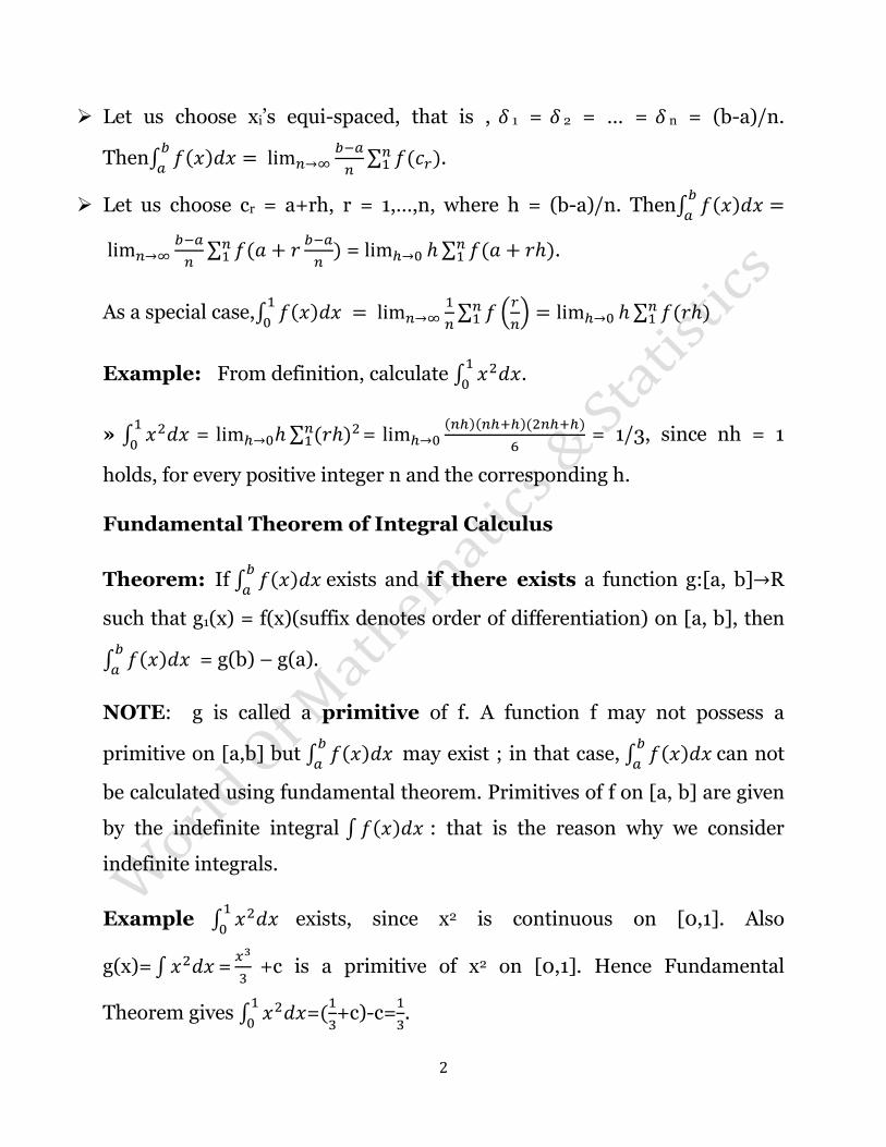
2
Let us choose xi’s equi-spaced, that is , 1 = 2 = … = n = (b-a)/n.
Then∫
∑
.
Let us choose cr = a+rh, r = 1,…,n, where h = (b-a)/n. Then∫
∑
= ∑ .
As a special case,∫
∑ (
) ∑
Example: From definition, calculate ∫
.
» ∫
= ∑
=
= 1/3, since nh = 1
holds, for every positive integer n and the corresponding h.
Fundamental Theorem of Integral Calculus
Theorem: If ∫
exists and if there exists a function g:[a, b] R
such that g1(x) = f(x)(suffix denotes order of differentiation) on [a, b], then
∫
= g(b) – g(a).
NOTE: g is called a primitive of f. A function f may not possess a
primitive on [a,b] but ∫
may exist ; in that case, ∫
can not
be calculated using fundamental theorem. Primitives of f on [a, b] are given
by the indefinite integral ∫ : that is the reason why we consider
indefinite integrals.
Example ∫
exists, since x2 is continuous on [0,1]. Also
g(x)= ∫ =
+c is a primitive of x2 on [0,1]. Hence Fundamental
Theorem gives ∫
=
+c)-c=
.
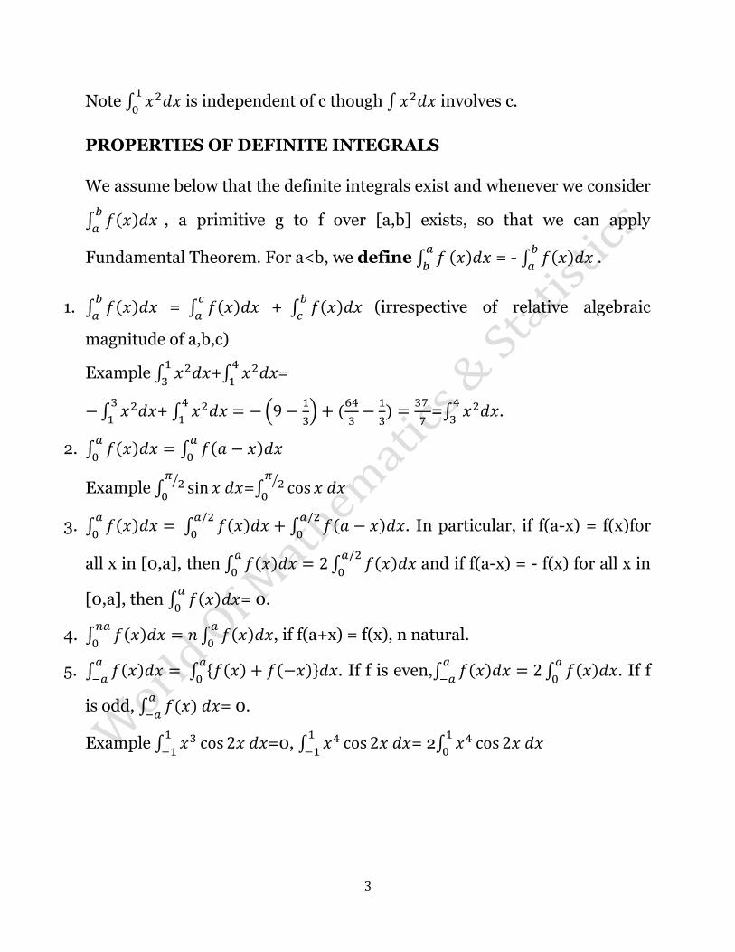
3
Note ∫
is independent of c though ∫ involves c.
PROPERTIES OF DEFINITE INTEGRALS
We assume below that the definite integrals exist and whenever we consider
∫
, a primitive g to f over [a,b] exists, so that we can apply
Fundamental Theorem. For a<b, we define ∫
= - ∫
.
1. ∫
= ∫
+ ∫
(irrespective of relative algebraic
magnitude of a,b,c)
Example ∫
+∫
=
∫
+ ∫
(
)
=∫
.
2. ∫ ∫
Example ∫
⁄
=∫
⁄
3. ∫ ∫ ∫
. In particular, if f(a-x) = f(x)for
all x in [0,a], then ∫ ∫
and if f(a-x) = - f(x) for all x in
[0,a], then ∫
= 0.
4. ∫ ∫
, if f(a+x) = f(x), n natural.
5. ∫ ∫ }
. If f is even,∫ ∫
. If f
is odd, ∫
= 0.
Example ∫
=0, ∫
= 2∫
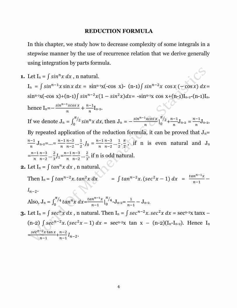
4
REDUCTION FORMULA
In this chapter, we study how to decrease complexity of some integrals in a
stepwise manner by the use of recurrence relation that we derive generally
using integration by parts formula.
1. Let In = ∫ , n natural.
In = ∫ = sinn-1x(-cos x)- (n-1)∫ =
sinn-1x(-cos x)+(n-1)∫ = -sinn-1x cos x+(n-1)In-2-(n-1)In.
hence In=
In-2.
If we denote Jn = ∫
⁄
then Jn =
⁄ +
Jn-2 =
Jn-2.
By repeated application of the reduction formula, it can be proved that Jn=
Jn-2=…=
=
, if n is even natural and Jn
=
=
, if n is odd natural.
2. Let In = ∫ , n natural.
Then In = ∫ = ∫ =
.
Also, Jn = ∫
⁄
=
⁄ -Jn-2=
Jn-2.
3. Let In = ∫ , n natural. Then In = ∫ = secn-2x tanx –
(n-2) ∫ = secn-2x tan x – (n-2)(In-In-2). Hence In
=
+
.
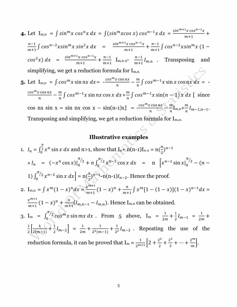
5
4. Let Im,n = ∫ = ∫ =
∫ =
∫
=
Im,n-2-
. Transposing and
simplifying, we get a reduction formula for Im,n.
5. Let Im,n = ∫ = -
∫ = -
∫ +
∫ [ since
cos nx sin x = sin nx cos x – sin(n-1)x] = -
Im,n+
.
Transposing and simplifying, we get a reduction formula for Im,n.
Illustrative examples
1. = ∫
and n>1, show that In+ n(n-1)In-2 = n
=
⁄ ∫
⁄
= n *
⁄
∫
⁄
+ = n
-n(n-1) . Hence the proof.
2. Im,n = ∫ =
∫ =
( . Hence Im,n can be obtained.
3. Im = ∫
⁄
. From 5 above, Im =
=
*
+ =
. Repeating the use of the
reduction formula, it can be proved that Im =
*
+.
6
IMPROPER INTEGRAL
When we consider the definite integral ∫
in earlier standards, we
implicitly assume two conditions to hold: (a) f is continuous on [a, b] or , to
that matter, at least the limit ∫ ∑
exists
independent of choice of points of subdivision xi and that of ci, for all i and
(b) the interval [a,b] is bounded. We want to extend the definition of
∫
when either (a) or (b) or both are not met. This extended
definition of definite integral is referred to as Improper Integrals.
Improper integrals can be of two types: (a) Type 1: interval of integration is
unbounded, (b) Type 2: integrand has a finite number of infinite
discontinuities in the interval of integration.
Definition of TYPE I improper integral ∫
,∫
and
∫
Let the function f be integrable in [a ,B], for every B>a. If ∫
exist finitely, we define ∫
= ∫
and we say ∫
exists or converges; otherwise ∫
diverges. Similarly, ∫
∫
(provided the limit exists) and ∫
∫ ∫
, a is any real, provided ∫
and ∫
exist separately.
7
Example: ∫
, ∫
√
. The range of integration of the integrals are
unbounded. For a>1, ∫
= 1-
and ∫
√
= 2(√ -1). Since (
)= 1 exists but ( (√ )) does not exist, hence the improper
integral ∫
converges and ∫
√
diverges.(compare areas below the
curves y = 1/x2 and y = 1/√ in diagram below)
Definition of TYPE II improper integral
Let f have an infinite discontinuity only at the point a (that is,
or and is continuous in (a, b].Then
we define ∫ ∫
,0<c<b-a, provided the limit
exists. Similarly, if f has an infinite discontinuity only at the point b and is
continuous in [a, b), then we define ∫ ∫
,
0<c<b-a, provided the limit exists. If f has an infinite discontinuity at d,
a<d<b, and is otherwise continuous in [a,b], we define ∫
∫ ∫
, provided both of ∫
and ∫
exist
separately.
Example: ∫
√
, ∫
. The integrands have an infinite discontinuity at
x=0. For 0<a<1, ∫
√ √
and ∫
. Since
√ = 2 exists but (
) does not exist, so ∫
√
converges whereas
∫
diverges. (Compare areas between x = a,0<a<1, and x = 1, below the
curves y = 1/x2 and y = 1/√ in diagram above)
8
Example: ∫
The integrand
is continuous everywhere but the interval of
integration is unbounded. Let a>o be fixed. ∫
=
∫
(
)
=
. Thus ∫
=
=
.
Example: ∫
√
=
.
The integrand has an infinite discontinuity at x = 3 and is continuous on
[0, 3). Let 0<a<3. Then ∫
√
= sin-1(a/3) . So ∫
√
=
(
)
. Hence ∫
√
=
.
Note : we can apply standard methods of integration, in particular method
of substitution, only to a proper integral and not directly to an improper
integral. Thus if we substitute z=1/x directly in the improper integral∫
,
we get a value -2 of the integral whereas it can be checked from definition
that the improper integral diverges.
TESTS FOR CONVERGENCE OF IMPROPER INTEGRALS
TYPE I INTEGRAL
Theorem: (Comparison test) Let f and g be integrable in [a, B], for every
B>a. Let g(x)>0, for all x ≥a. If
= c≠0, then the integrals
∫
and ∫
either both converge or both diverge. If c = 0 and
∫
converges , then ∫
converges.
9
Theorem: ( Let f be integrable in [a, B], for every B>a. Then
∫
converges if exists with >1 and ∫
diverges if exists and ≠0 with ≤ 1.
Example: ∫
converges by comparison test , since 0≤
for all
x 0,
and ∫
converges (need to prove!).
Example: ∫
converges by since
= 0 (verify
using L’Hospital’s rule) , = 2>1 and is continuous, and hence
integrable, in [0,B] for B>0.
Example: ∫
⁄
diverges, since
⁄ (
⁄
) = 1/3, = ½<1
and
⁄
is continuous, and hence integrable, in [0,B] for B>0.
TYPE II INTEGRAL
Theorem: (Comparison test) Let f and g be integrable in [c, b], for every c,
a<c<b. Let g(x)>0 , for all x, a<x≤b. If
≠0, then ∫
and
∫
both converge or both diverge. If
= 0 and
∫
converges, then ∫
converges.
Theorem: ( Let f be integrable in[c, b], for every c, a<c<b. Then
∫
converges if f(x) exists for and
∫
diverges if f(x) exists (≠0) for ≥1.
10
Example: ∫
√
converges , since
√ = 1, for <1
and
√ is continuous, and hence integrable, in [c,1]for 0<c<1.
Example: ∫
√
⁄ converges, since
⁄
√ = 1, for
and
√ is continuous, and hence integrable, in [1/2, c]for
1/2<c<1.
THE GAMMA AND BETA FUNCTIONS
Definition (Gamma function) For n>0, (n) = ∫
.
NOTE: Gamma function is an improper integral of type I. If 0<n<1, (n) is
also an improper integral of type II. We shall assume convergence of the
gamma function in our course of study.
Definition (Beta function) For m, n>0, (m,n) = ∫
NOTE: Beta function is an improper integral of type II if either m or n or
both lies between 0 and 1 strictly; otherwise it is a proper integral.
Properties of Gamma and Beta functions
1. For any a>0, ∫
= (n)/an.
» let 0<c<d. consider the proper integral I = ∫
. Let y = ax.
Then I = ∫
=
∫
. Thus lim I =
as
and d .

11
2. (n+1) = n (n)
» Let 0<c<d. using integration by parts on the proper integral I =
∫
, we get I = (
) ∫
=
(
+ ∫
, which tends to n (n) as c 0+ and d (by
use of L’Hospital’s rule). Hence the result.
3 (1) = 1 (can be verified easily)
(n+1) = n , for a natural n (follows from property 2 and 3)
4 (m,n) = (n,m) (follows using a substitution y = 1-x after passing to a
proper integral)
5 (m,n) =2∫
⁄
(follows using a substitution x = sin2
after passing to a proper integral)
6 (
,
)= (follows from definition)
7
8 (
) √
9 For 0<m<1, (m) (1-m) = cosec(m
Example: ∫
√
.
» The range of integration of the given integral is unbounded but the
integrand is continuous everywhere. For 0<a, ∫
=
∫
(substituting y = x2 in the proper integral ). Thus ∫
=
∫
=
∫
=
(
) = √ .
12
Example: ∫
.
» The integrand has an infinite discontinuity at x = 1.Let 0<c<1.
Substituting x3 = sin in the proper integral ∫
⁄
, ∫
⁄
=
∫
⁄
⁄ . Since ∫
⁄
=
(5/3,1/3) =
(
)
=
.
(
)
=
(
) (
)
.
DOUBLE INTEGRAL
Let f(x,y) be a bounded function of two independent variables x and y
defined over a closed rectangular region R: a≤x≤b; c≤y≤d. we take
partitions {a = x0,x1,…,xr-1,xr,…,xn = b} of [a,b] and {c = y0,y1,…,ys-1,ys,…,ym =
d}. These partitions divides the rectangle R into mn number of
subrectangles Rij(1≤i≤n, 1≤j≤m). Let us choose arbitrarily (
and , 1≤i≤n, 1≤j≤m. the volume of the
parallelepiped with base Rij and altitude f( is f( (xi-xi-1)(yj-yj-1).
∑ ( ) , sum of the volumes of all the
parallelepipeds erected over all of the Rij’s, gives an approximation of the
volume enclosed by the curve and the planes x = a,x = b, y = c, y = d and z =
0. The approximation can be improved by increasing number of
subrectangles into which R is divided into. Thus the limit
∑ ( ) , provided it exists, gives the
volume and is represented by ∬
.
13
NOTE: Every continuous function is integrable over any rectangle.
Theorem: (equivalence of double integrals with repeated
integrals) If ∬
exists over a rectangle R: a≤x≤b; c≤y≤d and
∫
exists for each value of y in [c,d], then the repeated integral
∫ ∫
exists and is equal to ∬
Example: Evaluate ∬
over R:0≤x≤
, 0≤y≤
Sol: sin(x+y) is continuous on R, so the double integral ∬
exists . Evaluating given double integral in terms of repeated
integrals,
∬
= ∫ ∫
⁄
⁄
= ∫
⁄
∫
= 2.
EVALUATION OF AREA
Cartesian co-ordinate
It has already been seen that area of the region bounded by the curve y =
f(x), lines x = a, x = b and y = 0 is given by ∫
, provided it exists.
Similarly area of the region bounded by the curve x = g(y), lines y = c, y = d
and x = 0 is given by ∫
, provided it exists. We can define F:[a,b] R
by F(t)=∫
,a≤t≤b.

14
Example: Find the area of the bounded region bounded by the curves y =
x2 and x = y2.
Sol: On solving the given equations of the curves, the point of intersection
of the two curves are (0,0) and (4,4). Thus required area = ∫ √
∫
.
Example: Find the area of the loop formed by the curve y2 = x(x-2)2
Sol: The abscissa of points of intersection of the curve with the x-axis are
given by y = 0, that is, x = 0,2,2. For x<0, no real value of y satisfy the
equation. Hence no part of the curve exist corresponding to x<0.
Corresponding to each x-value satisfying 0<x<2, there exist two values of y,
equal in magnitude and opposite in sign. Thus between x = 0 and x = 2, the
curve is symmetric about the x-axis and a loop is formed thereby. For x>2,
y as x . the required area = 2∫ √
(by symmetry of the
curve about x-axis).
Example: Prove that area included in a circle of radius r unit is r2 square
unit.
Sol: We can choose two perpendicular straight lines passing through the
centre of the circle as co-ordinate axes. With reference to such a co-ordinate
system, equation of the circle is y = ±√ .Curve is symmetric about the
axes .Thus required area = 4∫ √
dx.
15
Polar Coordinates:
The area of the region bounded by the curve r = f( ) , the radius vector
, is given by
∫
.
Example: Find the area enclosed by the cardioide r = a(1+ cos )
Sol: As varies from 0 to
, r decreases continuously from 2a to a. When
further increases from
to , r decreases further from a to 0. Also the
curve is symmetric about the initial line (since the equation of the curve
remains unaffected on replacing by – . Hence the area enclosed by the
curve = 2.
∫
.
Example: Find the area enclosed by the cardioide r = a(1+ cos ) and r =
a(1- cos )
Sol: The vectorial angle corresponding the points of intersection of the
curves are
and =-
. Because of the symmetry of the curves about the
initial line,
, =-
and , required area is 4.
∫
⁄
.
1
AN INTRODUCTION TO STATISTICS
"Status"-"State"->"Statistics". STEPS AT A GLANCE : Collection of Data-> Summarisation of Data-> Analysis of Data-> Interpretation of Data towards a VALID DECISION. WHAT IS THE MAIN PROBLEM IN STATISTICS? Given a sample(a set of outcomes),we are to say(infer) about the population or the model.Statistics primarily deals with situations in which the occurrence of some event can't. be predicted with certainty. WHAT ARE THE MAJOR OBJECTIVES OF STATISTICS? 1. To make inference about a population from an analysis of information contained in the sample data. 2. To make assessments of the extent of uncertainty involved in these inferences. A third objective,no less important,is to design the process & the extent of sampling so that the observations from a basis for drawing valid & accurate inferences. GIVE THE DEFINITION OF STATISTICS? "STATISTICS" is a science of decision making on the basis of sample observations drawn from a population under uncertainty. That is, it is a mathematical discipline concerned with collection of data,summarisation of data,analysis of data & interpretation of data toward a valid decision. Encyclopaedia Americana :- As a name of a field of study, Statistics refers to the science & arts of obtaining & analysing quantitative data with a view to make sound inferences in the face of uncertainty. Encyclopaedia Britannica:- As is commonly understood now a days, Statistics is a mathematical discipline concerned with the study of masses of quantitative data of any kind. WHAT IS THE MEANING OF THE TERM 'STATISTICS'? As a singular noun it refers the science of collecting,analysing & interpreting numerical data relating to an aggregate of individuals. As a plural noun it denotes the numerical & quantitative information,e.g., labour statistics,vital statistics. IS STATISTICS A SCIENCE? Any Science has for its objectives the formulation of laws for explaining phenomena in some part of the real world with a deterministic view-point. As Kendall explained ," Statistics is the branch of scientific method which deals with the data obtained by counting or measuring the properties of population of natural phenomena". Indeed, we can call Statistical Methodology as Scientific Method. It is noted that STATISTICS is sometimes called the study of variation, i.e., a population or group without any variation &
2
uncertainty is no interest to Statistics. So, Statistics is the scientific methodology which deals with the collection,classification & tabulation of numerical facts as a basis for explanation,description & comparison of social phenomena. DEFINE THE TERMS: STATISTICAL DATA,POPULATION,SAMPLE. Statistical Data:- The numerical data or measurements obtained in case of an enquiry into a phenomenon,marked by uncertainty & variability,constitute Statistical Data. Uncertainty & variability are two major characteristics of Statistical data. Not all quantitative data is statistical data. Example of statistical data--Suppose we study the 'Heights of students in a particular college'.Here we can't predict the height of an individual with certainty & there will be variation in heights of students. Counter Example:--Multiplication table in a tabular form is a quantitative data,but since there is no uncertainty & variability involved in the data so it's not a Statistical Data. Population:- A set or group of observations relating to a phenomenon under statistical investigation is known as statistical population or simply population. However,the term 'population' implies an aggregate or collection of measurements on a given variable(s). Population is said to be finite or infinite according to whether the set contains a finite or infinite number of observations. Example-Measurements of heights in your college. Note that: I. The characteristics of a population are called parameters. II.A population contains finite or infinite no of observations on a given variable(s). Sample :- The set of data actually collected through a process of observation from selected items of any source is called a Sample. However, "Sample" is a subset of population or a true representation of population. Example- Measurements of heights of students of Statistics department in your college. Note that:- I. The characteristics of sample are called as Statistic. II. A sample is taken in order to gather information about a population. WRITE DOWN THE DRAWBACKS OF STATISTICS? Limitations of Statistics: I. Statistics deals with quantitative data only. II. Statistical law holds good only for aggregate of items or average individuals. It may not true for a particular individual or item. III. Inadequate knowledge of data interpretation may lead to invalid decision. There are some sayings: "There are there kinds of lies--lies,white lies & Statistics" , "Figure won't lie,but liars figure" , "Statistics is like a clay of which you can make a god or a devil". COMMENT ON THE FOLLOWING: "In a study of ages & professions of deceased men, it was found that the profession with the lowest average age of death was 'student' .So it appears that student profession is very dangerous." It is obvious that every professional must have some basic education & it happens that the average age of every professional men must be higher than the age of the students. But it can happen that profession with lowest age of death was student . So the given statement is TRUE. But the conclusion made from the fact is incorrect . It can never be told that the student profession is dangerous. To conclude properly,we must have data for computing the proportions or percentages of deceased men in different professions. Therefore the conclusion
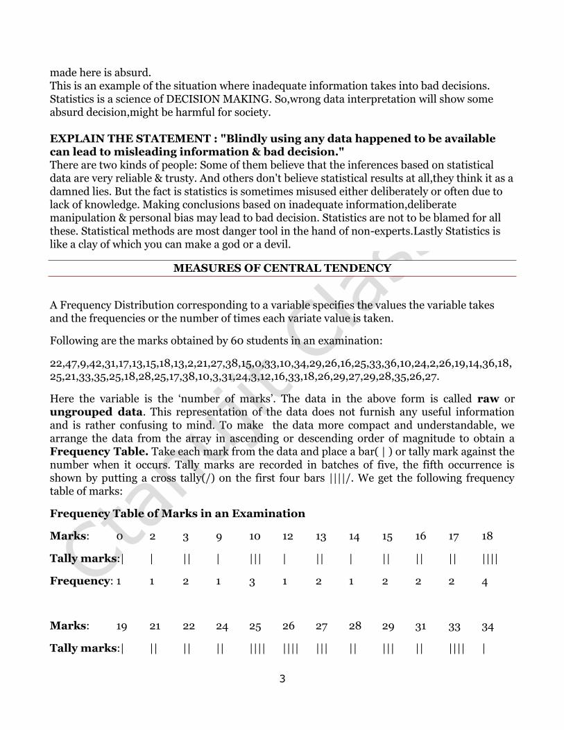
3
made here is absurd. This is an example of the situation where inadequate information takes into bad decisions. Statistics is a science of DECISION MAKING. So,wrong data interpretation will show some absurd decision,might be harmful for society. EXPLAIN THE STATEMENT : "Blindly using any data happened to be available can lead to misleading information & bad decision." There are two kinds of people: Some of them believe that the inferences based on statistical data are very reliable & trusty. And others don't believe statistical results at all,they think it as a damned lies. But the fact is statistics is sometimes misused either deliberately or often due to lack of knowledge. Making conclusions based on inadequate information,deliberate manipulation & personal bias may lead to bad decision. Statistics are not to be blamed for all these. Statistical methods are most danger tool in the hand of non-experts.Lastly Statistics is like a clay of which you can make a god or a devil.
MEASURES OF CENTRAL TENDENCY
A Frequency Distribution corresponding to a variable specifies the values the variable takes and the frequencies or the number of times each variate value is taken.
Following are the marks obtained by 60 students in an examination:
22,47,9,42,31,17,13,15,18,13,2,21,27,38,15,0,33,10,34,29,26,16,25,33,36,10,24,2,26,19,14,36,18,25,21,33,35,25,18,28,25,17,38,10,3,31,24,3,12,16,33,18,26,29,27,29,28,35,26,27.
Here the variable is the ‘number of marks’. The data in the above form is called raw or ungrouped data. This representation of the data does not furnish any useful information and is rather confusing to mind. To make the data more compact and understandable, we arrange the data from the array in ascending or descending order of magnitude to obtain a Frequency Table. Take each mark from the data and place a bar( | ) or tally mark against the number when it occurs. Tally marks are recorded in batches of five, the fifth occurrence is shown by putting a cross tally(/) on the first four bars ||||/. We get the following frequency table of marks:
Frequency Table of Marks in an Examination
Marks: 0 2 3 9 10 12 13 14 15 16 17 18
Tally marks:| | || | ||| | || | || || || ||||
Frequency: 1 1 2 1 3 1 2 1 2 2 2 4
Marks: 19 21 22 24 25 26 27 28 29 31 33 34
Tally marks:| || || || |||| |||| ||| || ||| || |||| |
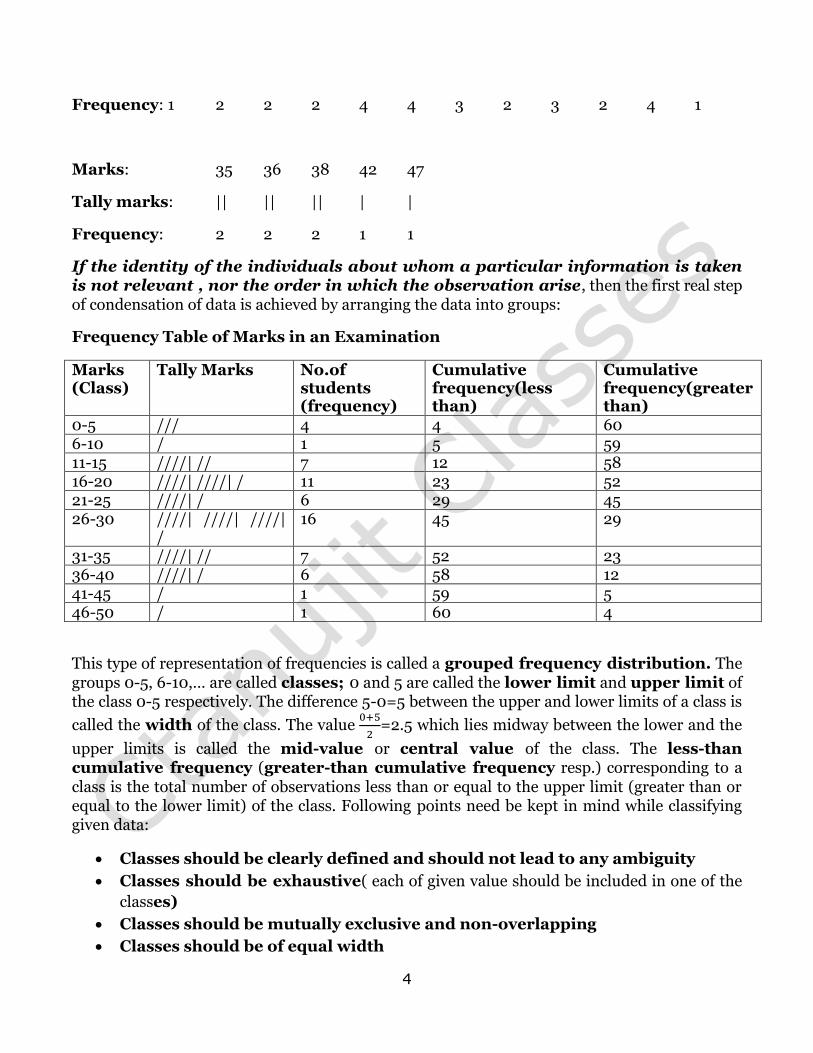
4
Frequency: 1 2 2 2 4 4 3 2 3 2 4 1
Marks: 35 36 38 42 47
Tally marks: || || || | |
Frequency: 2 2 2 1 1
If the identity of the individuals about whom a particular information is taken is not relevant , nor the order in which the observation arise, then the first real step of condensation of data is achieved by arranging the data into groups:
Frequency Table of Marks in an Examination
Marks (Class)
Tally Marks No.of students (frequency)
Cumulative frequency(less than)
Cumulative frequency(greater than)
0-5 /// 4 4 60 6-10 / 1 5 59 11-15 ////| // 7 12 58 16-20 ////| ////| / 11 23 52 21-25 ////| / 6 29 45 26-30 ////| ////| ////|
/ 16 45 29
31-35 ////| // 7 52 23 36-40 ////| / 6 58 12 41-45 / 1 59 5 46-50 / 1 60 4
This type of representation of frequencies is called a grouped frequency distribution. The groups 0-5, 6-10,… are called classes; 0 and 5 are called the lower limit and upper limit of the class 0-5 respectively. The difference 5-0=5 between the upper and lower limits of a class is
called the width of the class. The value
=2.5 which lies midway between the lower and the
upper limits is called the mid-value or central value of the class. The less-than cumulative frequency (greater-than cumulative frequency resp.) corresponding to a class is the total number of observations less than or equal to the upper limit (greater than or equal to the lower limit) of the class. Following points need be kept in mind while classifying given data:
Classes should be clearly defined and should not lead to any ambiguity
Classes should be exhaustive( each of given value should be included in one of the
classes)
Classes should be mutually exclusive and non-overlapping
Classes should be of equal width
5
Number of classes should neither be too large nor too small; preferably it
should lie between 5 and 15.
NOTE: A variable, which can take any numerical value within certain range , is called a continuous variable. Consider frequency distribution of the continuous variable of ages in years of students in a college. We cannot arrange the data in age groups 16-20,21-25 etc. since there can be students having ages between 20 and 21 years. If the original ‘inclusive’ class
intervals( of the form [a,b]) are ,say, 16-20,21-25,…, we calculate the adjustment
(lower limit
of succeeding class-upper limit of a class)=
(21-20)=.5 and change the class intervals to
‘exclusive’ type([a,b)): 15.5-20.5, 20.5-25.5,…. It is understood that age of students whose age
is 15.5 and < 20.5 are included in the class interval 15.5-20.5.
Comparison of Frequency Distributions
It is frequently necessary to compare two frequency distributions. If they are of different types , a precise comparison is difficult and is usually not required. If they are of same type, a comparison can be made in terms of values of the following four types of measures:
Measure of location or central tendency gives a single value around which largest
number of values of the variate tend to cluster.
The scale parameter or measure of dispersion gives the degree of scatter about
the central value. It measures variability or lack of homogeneity of data.
Measure of skewness measuring degree of departure from symmetry
Measure of Kurtosis measuring degree of ‘flatness’ of the ‘top’ as compared with the
‘normal’ curve.
Characteristics of a good measure of Central Tendency
It should be based on all observations
It should not be affected much by extreme values
It should be rigidly defined
It should be easily understandable and easy to calculate
It should be amenable to algebraic treatment
It should be least affected by fluctuation of sampling: if a number of samples of same
size are drawn from a population, the measure of central tendency having minimum
variation among the different calculated values should be preferred.
Different Measures of Central Tendency
Arithmetic Mean
Geometric Mean
Harmonic Mean
Median and Quartiles
Mode
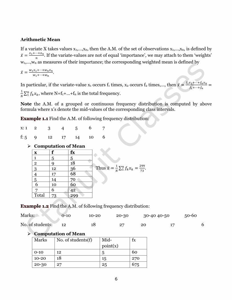
6
Arithmetic Mean
If a variate X takes values x1,…,xn, then the A.M. of the set of observations x1,…,xn, is defined by
. If the variate-values are not of equal ‘importance’, we may attach to them ‘weights’
w1,…,wn as measures of their importance; the corresponding weighted mean is defined by
.
In particular, if the variate-value x1 occurs f1 times, x2 occurs f2 times,…, then
∑
, where N=f1+…+fn is the total frequency.
Note the A.M. of a grouped or continuous frequency distribution is computed by above formula where x’s denote the mid-values of the corresponding class intervals.
Find the A.M. of following frequency distribution:
x: 1 2 3 4 5 6 7
f: 5 9 12 17 14 10 6
Computation of Mean
Thus
∑
.
Find the A.M. of following frequency distribution:
Marks: 0-10 10-20 20-30 30-40 40-50 50-60
No. of students: 12 18 27 20 17 6
Computation of Mean
Marks No. of students(f) Mid-
point(x)
fx
0-10 12 5 60
10-20 18 15 270
20-30 27 25 675
x f fx 1 5 5 2 9 18 3 12 36 4 17 68 5 14 70 6 10 60 7 6 42 Total 73 299
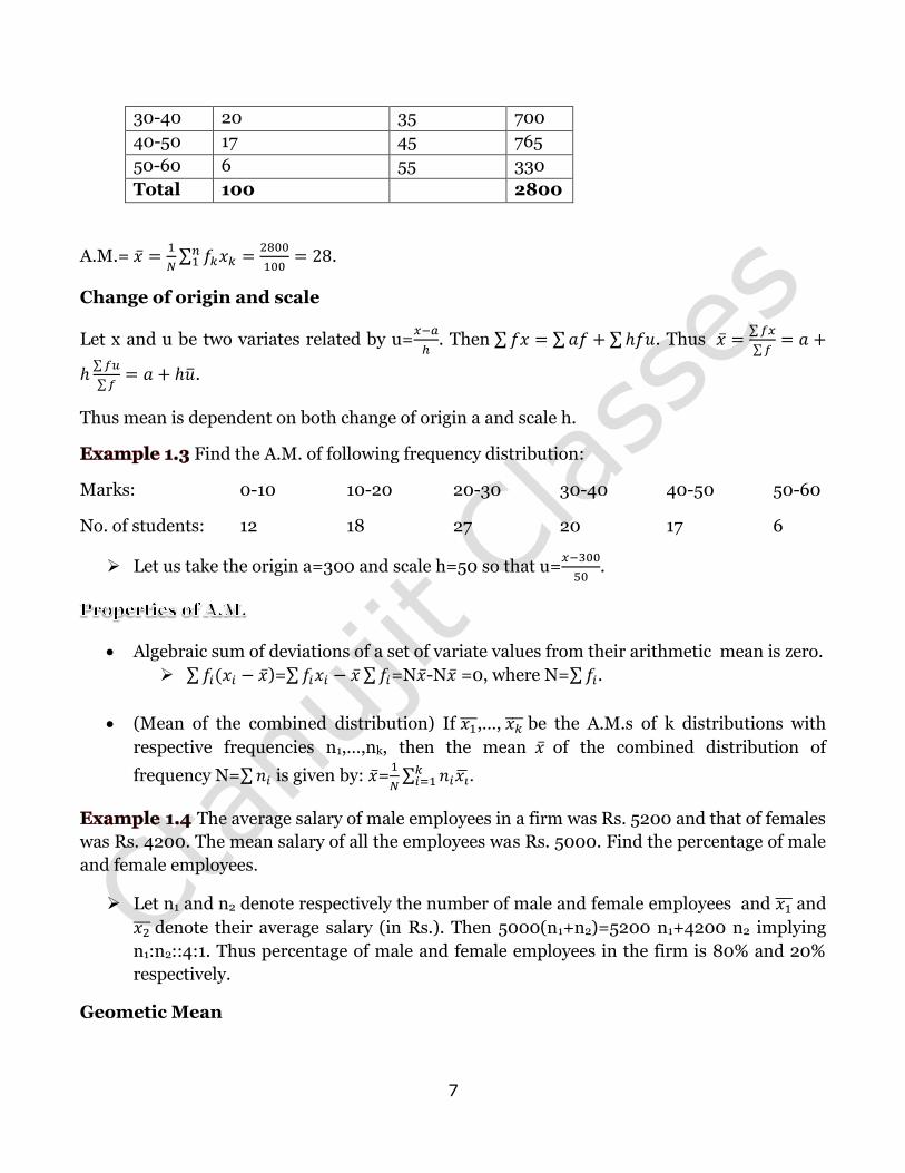
7
30-40 20 35 700
40-50 17 45 765
50-60 6 55 330
Total 100 2800
A.M.=
∑
.
Change of origin and scale
Let x and u be two variates related by u=
. Then ∑ ∑ ∑ . Thus
∑
∑
∑
∑ .
Thus mean is dependent on both change of origin a and scale h.
Find the A.M. of following frequency distribution:
Marks: 0-10 10-20 20-30 30-40 40-50 50-60
No. of students: 12 18 27 20 17 6
Let us take the origin a=300 and scale h=50 so that u=
.
Algebraic sum of deviations of a set of variate values from their arithmetic mean is zero.
∑ )=∑ ∑ =N -N =0, where N=∑ .
(Mean of the combined distribution) If ,…, be the A.M.s of k distributions with
respective frequencies n1,…,nk, then the mean of the combined distribution of
frequency N=∑ is given by: =
∑
.
The average salary of male employees in a firm was Rs. 5200 and that of females
was Rs. 4200. The mean salary of all the employees was Rs. 5000. Find the percentage of male
and female employees.
Let n1 and n2 denote respectively the number of male and female employees and and
denote their average salary (in Rs.). Then 5000(n1+n2)=5200 n1+4200 n2 implying
n1:n2::4:1. Thus percentage of male and female employees in the firm is 80% and 20%
respectively.
Geometic Mean
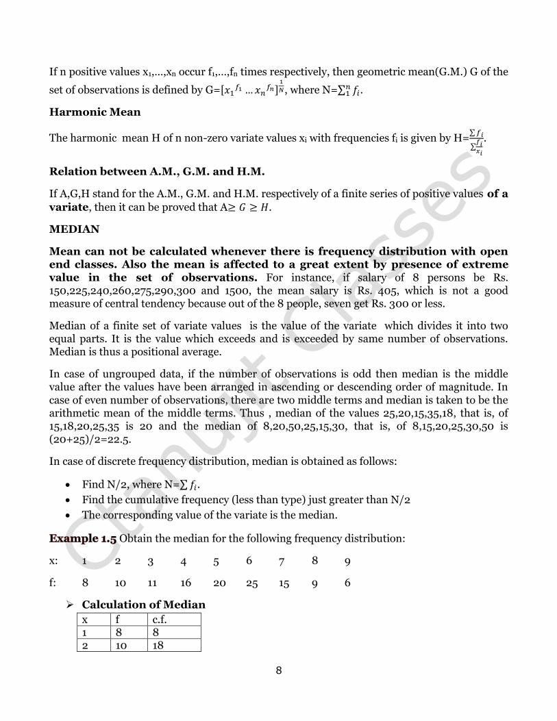
8
If n positive values x1,…,xn occur f1,…,fn times respectively, then geometric mean(G.M.) G of the
set of observations is defined by G=[
]
, where N=∑ .
Harmonic Mean
The harmonic mean H of n non-zero variate values xi with frequencies fi is given by H=∑
∑
.
Relation between A.M., G.M. and H.M.
If A,G,H stand for the A.M., G.M. and H.M. respectively of a finite series of positive values of a
variate, then it can be proved that A .
MEDIAN
Mean can not be calculated whenever there is frequency distribution with open end classes. Also the mean is affected to a great extent by presence of extreme value in the set of observations. For instance, if salary of 8 persons be Rs. 150,225,240,260,275,290,300 and 1500, the mean salary is Rs. 405, which is not a good measure of central tendency because out of the 8 people, seven get Rs. 300 or less.
Median of a finite set of variate values is the value of the variate which divides it into two equal parts. It is the value which exceeds and is exceeded by same number of observations. Median is thus a positional average.
In case of ungrouped data, if the number of observations is odd then median is the middle value after the values have been arranged in ascending or descending order of magnitude. In case of even number of observations, there are two middle terms and median is taken to be the arithmetic mean of the middle terms. Thus , median of the values 25,20,15,35,18, that is, of 15,18,20,25,35 is 20 and the median of 8,20,50,25,15,30, that is, of 8,15,20,25,30,50 is (20+25)/2=22.5.
In case of discrete frequency distribution, median is obtained as follows:
Find N/2, where N=∑ .
Find the cumulative frequency (less than type) just greater than N/2
The corresponding value of the variate is the median.
Obtain the median for the following frequency distribution:
x: 1 2 3 4 5 6 7 8 9
f: 8 10 11 16 20 25 15 9 6
Calculation of Median
x f c.f. 1 8 8 2 10 18
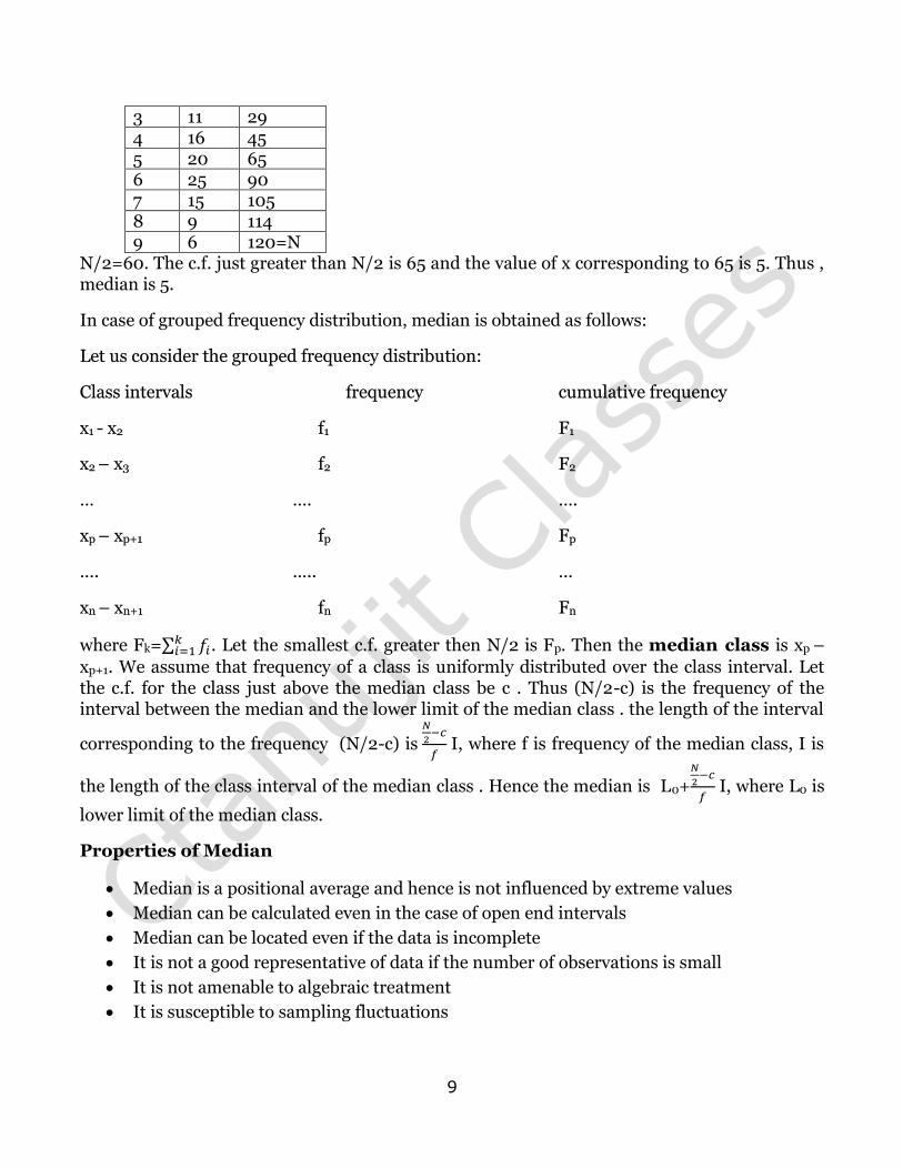
9
3 11 29 4 16 45 5 20 65 6 25 90 7 15 105 8 9 114 9 6 120=N
N/2=60. The c.f. just greater than N/2 is 65 and the value of x corresponding to 65 is 5. Thus , median is 5.
In case of grouped frequency distribution, median is obtained as follows:
Let us consider the grouped frequency distribution:
Class intervals frequency cumulative frequency
x1 - x2 f1 F1
x2 – x3 f2 F2
… …. ….
xp – xp+1 fp Fp
…. ….. …
xn – xn+1 fn Fn
where Fk=∑ . Let the smallest c.f. greater then N/2 is Fp. Then the median class is xp –
xp+1. We assume that frequency of a class is uniformly distributed over the class interval. Let the c.f. for the class just above the median class be c . Thus (N/2-c) is the frequency of the interval between the median and the lower limit of the median class . the length of the interval
corresponding to the frequency (N/2-c) is
I, where f is frequency of the median class, I is
the length of the class interval of the median class . Hence the median is L0+
I, where L0 is
lower limit of the median class.
Properties of Median
Median is a positional average and hence is not influenced by extreme values
Median can be calculated even in the case of open end intervals
Median can be located even if the data is incomplete
It is not a good representative of data if the number of observations is small
It is not amenable to algebraic treatment
It is susceptible to sampling fluctuations
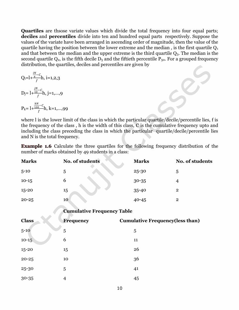
10
Quartiles are thsose variate values which divide the total frequency into four equal parts; deciles and percentiles divide into ten and hundred equal parts respectively. Suppose the values of the variate have been arranged in ascending order of magnitude, then the value of the quartile having the position between the lower extreme and the median , is the first quartile Q1 and that between the median and the upper extreme is the third quartile Q3. The median is the second quartile Q2, is the fifth decile D5 and the fiftieth percentile P50. For a grouped frequency distribution, the quartiles, deciles and percentiles are given by
Qi=l+
h, i=1,2,3
Dj= l+
h, j=1,…,9
Pk= l+
h, k=1,…,99
where l is the lower limit of the class in which the particular quartile/decile/percentile lies, f is the frequency of the class , h is the width of this class, C is the cumulative frequency upto and including the class preceding the class in which the particular quartile/decile/percentile lies and N is the total frequency.
Calculate the three quartiles for the following frequency distribution of the number of marks obtained by 49 students in a class:
Marks No. of students Marks No. of students
5-10 5 25-30 5
10-15 6 30-35 4
15-20 15 35-40 2
20-25 10 40-45 2
Cumulative Frequency Table
Class Frequency Cumulative Frequency(less than)
5-10 5 5
10-15 6 11
15-20 15 26
20-25 10 36
25-30 5 41
30-35 4 45
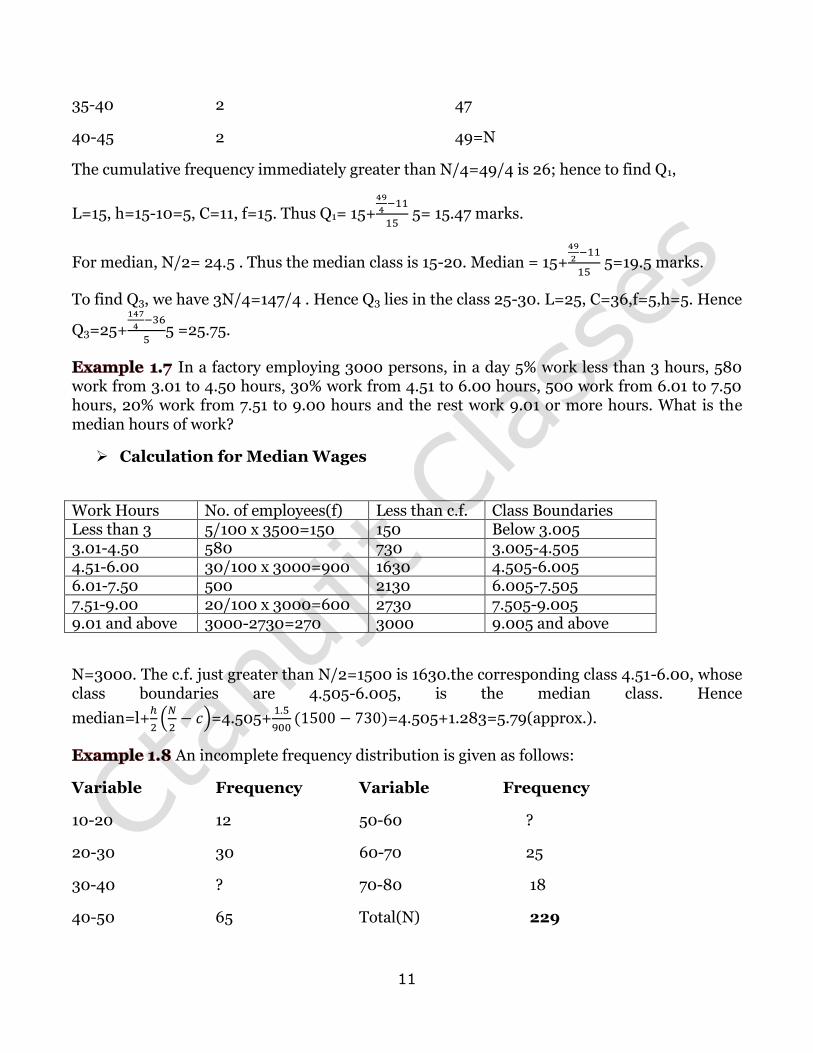
11
35-40 2 47
40-45 2 49=N
The cumulative frequency immediately greater than N/4=49/4 is 26; hence to find Q1,
L=15, h=15-10=5, C=11, f=15. Thus Q1= 15+
5= 15.47 marks.
For median, N/2= 24.5 . Thus the median class is 15-20. Median = 15+
5=19.5 marks.
To find Q3, we have 3N/4=147/4 . Hence Q3 lies in the class 25-30. L=25, C=36,f=5,h=5. Hence
Q3=25+
5 =25.75.
In a factory employing 3000 persons, in a day 5% work less than 3 hours, 580 work from 3.01 to 4.50 hours, 30% work from 4.51 to 6.00 hours, 500 work from 6.01 to 7.50 hours, 20% work from 7.51 to 9.00 hours and the rest work 9.01 or more hours. What is the median hours of work?
Calculation for Median Wages
Work Hours No. of employees(f) Less than c.f. Class Boundaries Less than 3 5/100 x 3500=150 150 Below 3.005 3.01-4.50 580 730 3.005-4.505 4.51-6.00 30/100 x 3000=900 1630 4.505-6.005 6.01-7.50 500 2130 6.005-7.505 7.51-9.00 20/100 x 3000=600 2730 7.505-9.005 9.01 and above 3000-2730=270 3000 9.005 and above
N=3000. The c.f. just greater than N/2=1500 is 1630.the corresponding class 4.51-6.00, whose class boundaries are 4.505-6.005, is the median class. Hence
median=l+
(
)=4.505+
=4.505+1.283=5.79(approx.).
An incomplete frequency distribution is given as follows:
Variable Frequency Variable Frequency
10-20 12 50-60 ?
20-30 30 60-70 25
30-40 ? 70-80 18
40-50 65 Total(N) 229
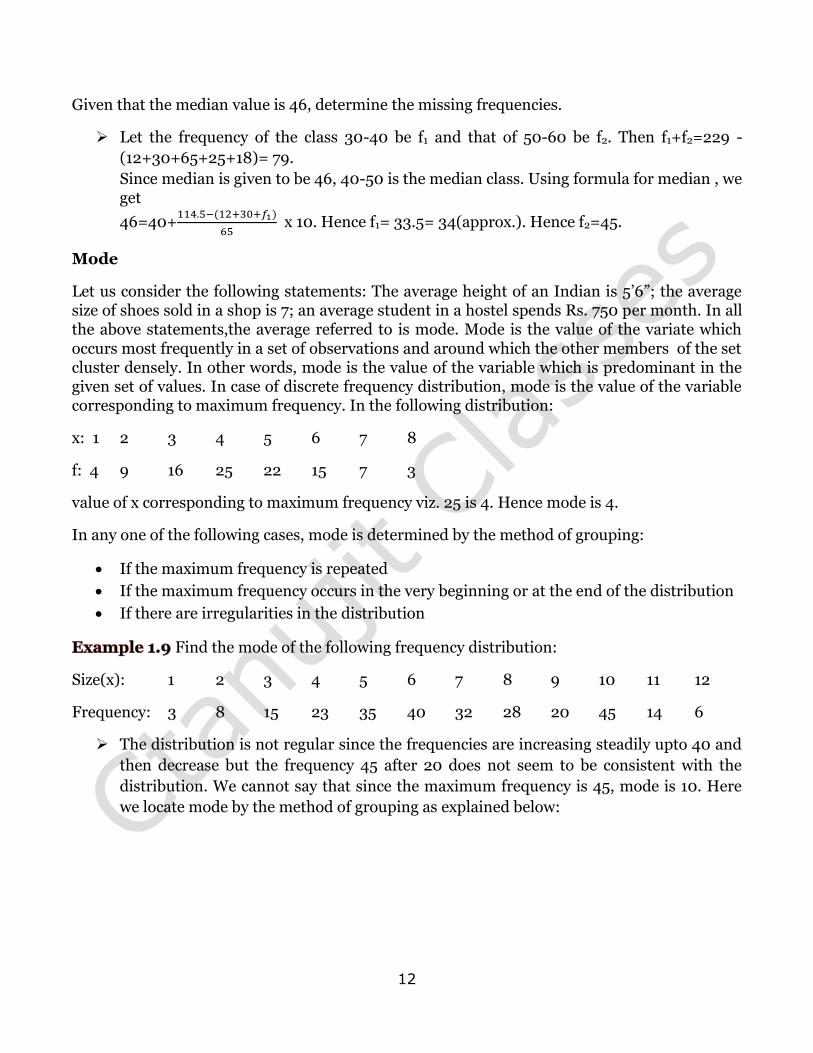
12
Given that the median value is 46, determine the missing frequencies.
Let the frequency of the class 30-40 be f1 and that of 50-60 be f2. Then f1+f2=229 -
(12+30+65+25+18)= 79.
Since median is given to be 46, 40-50 is the median class. Using formula for median , we get
46=40+
x 10. Hence f1= 33.5= 34(approx.). Hence f2=45.
Mode
Let us consider the following statements: The average height of an Indian is 5’6”; the average size of shoes sold in a shop is 7; an average student in a hostel spends Rs. 750 per month. In all the above statements,the average referred to is mode. Mode is the value of the variate which occurs most frequently in a set of observations and around which the other members of the set cluster densely. In other words, mode is the value of the variable which is predominant in the given set of values. In case of discrete frequency distribution, mode is the value of the variable corresponding to maximum frequency. In the following distribution:
x: 1 2 3 4 5 6 7 8
f: 4 9 16 25 22 15 7 3
value of x corresponding to maximum frequency viz. 25 is 4. Hence mode is 4.
In any one of the following cases, mode is determined by the method of grouping:
If the maximum frequency is repeated
If the maximum frequency occurs in the very beginning or at the end of the distribution
If there are irregularities in the distribution
Find the mode of the following frequency distribution:
Size(x): 1 2 3 4 5 6 7 8 9 10 11 12
Frequency: 3 8 15 23 35 40 32 28 20 45 14 6
The distribution is not regular since the frequencies are increasing steadily upto 40 and
then decrease but the frequency 45 after 20 does not seem to be consistent with the
distribution. We cannot say that since the maximum frequency is 45, mode is 10. Here
we locate mode by the method of grouping as explained below:
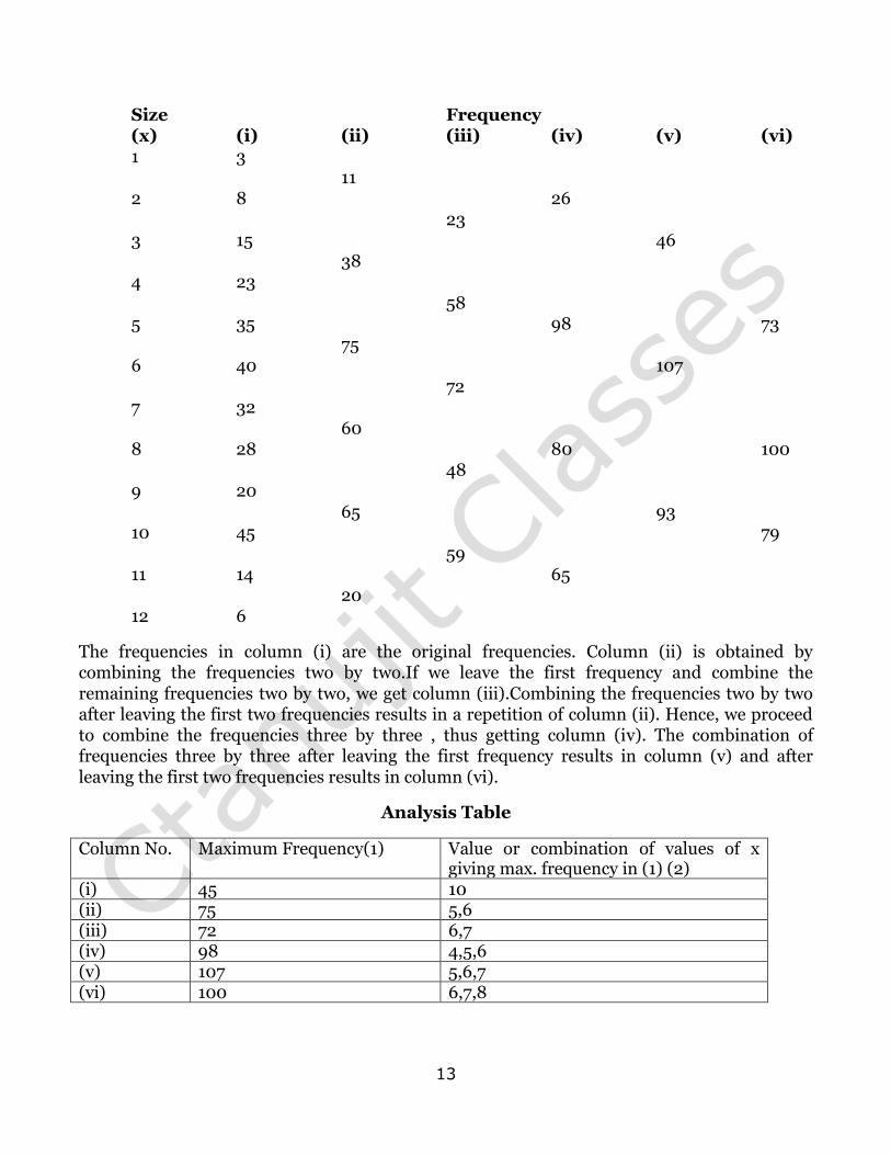
13
Size Frequency (x) (i) (ii) (iii) (iv) (v) (vi) 1 3 11 2 8 26 23 3 15 46 38 4 23 58 5 35 98 73 75 6 40 107 72 7 32 60 8 28 80 100 48 9 20 65 93 10 45 79 59 11 14 65 20 12 6
The frequencies in column (i) are the original frequencies. Column (ii) is obtained by combining the frequencies two by two.If we leave the first frequency and combine the remaining frequencies two by two, we get column (iii).Combining the frequencies two by two after leaving the first two frequencies results in a repetition of column (ii). Hence, we proceed to combine the frequencies three by three , thus getting column (iv). The combination of frequencies three by three after leaving the first frequency results in column (v) and after leaving the first two frequencies results in column (vi).
Analysis Table
Column No. Maximum Frequency(1) Value or combination of values of x giving max. frequency in (1) (2)
(i) 45 10 (ii) 75 5,6 (iii) 72 6,7 (iv) 98 4,5,6 (v) 107 5,6,7 (vi) 100 6,7,8
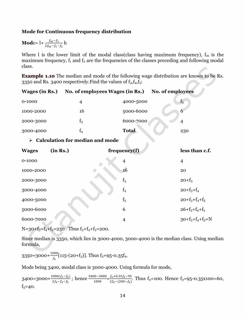
14
Mode for Continuous frequency distribution
Mode= l+
h
Where l is the lower limit of the modal class(class having maximum frequency), fm is the maximum frequency, f1 and f2 are the frequencies of the classes preceding and following modal class.
The median and mode of the following wage distribution are known to be Rs. 3350 and Rs. 3400 respectively.Find the values of f3,f4,f5:
Wages (in Rs.) No. of employees Wages (in Rs.) No. of employees
0-1000 4 4000-5000 f5
1000-2000 16 5000-6000 6
2000-3000 f3 6000-7000 4
3000-4000 f4 Total 230
Calculation for median and mode
Wages (in Rs.) frequency(f) less than c.f.
0-1000 4 4
1000-2000 16 20
2000-3000 f3 20+f3
3000-4000 f4 20+f3+f4
4000-5000 f5 20+f3+f4+f5
5000-6000 6 26+f3+f4+f5
6000-7000 4 30+f3+f4+f5=N
N=30+f3+f4+f5=230 . Thus f3+f4+f5=200.
Since median is 3350, which lies in 3000-4000, 3000-4000 is the median class. Using median formula,
3350=3000+
[115-(20+f3)]. Thus f3=95-0.35f4.
Mode being 3400, modal class is 3000-4000. Using formula for mode,
3400=3000+
; hence
=
. Thus f4=100. Hence f3=95-0.35x100=60,
f5=40.
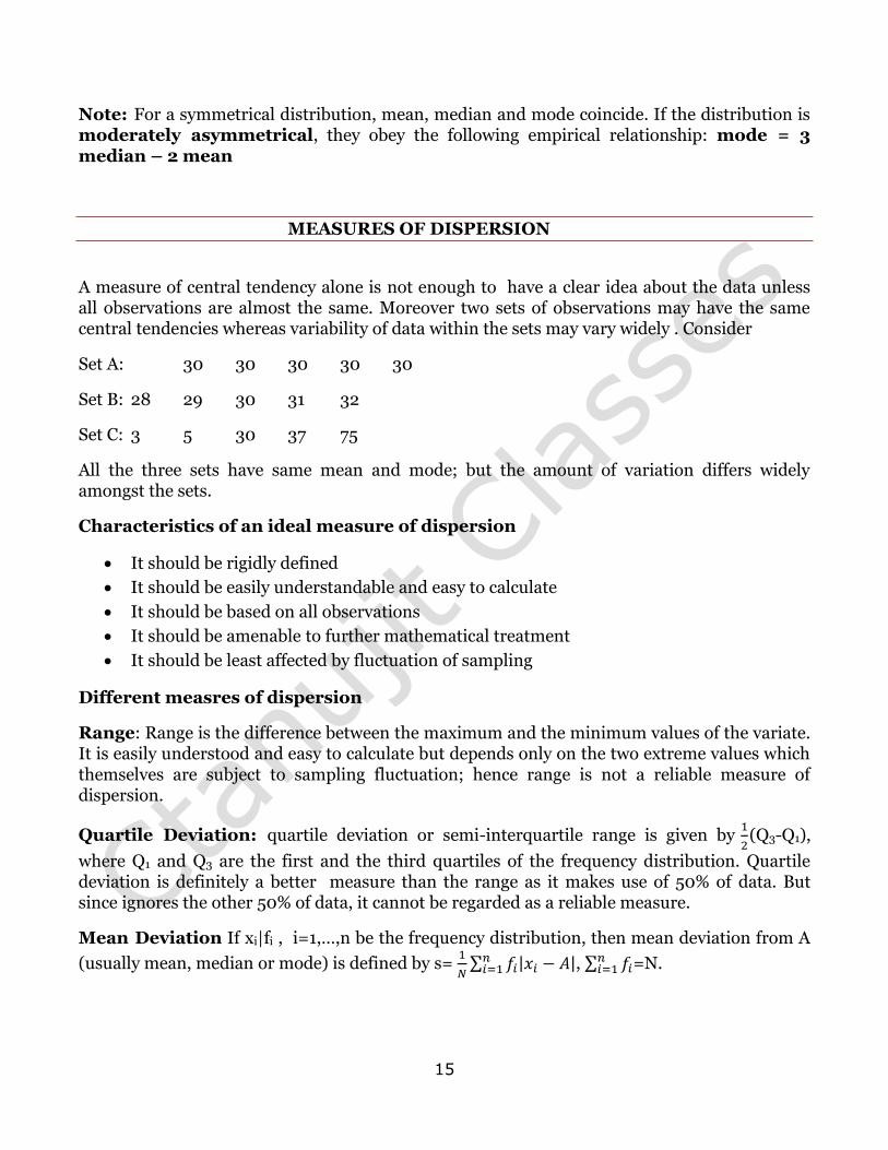
15
Note: For a symmetrical distribution, mean, median and mode coincide. If the distribution is moderately asymmetrical, they obey the following empirical relationship: mode = 3 median – 2 mean
MEASURES OF DISPERSION
A measure of central tendency alone is not enough to have a clear idea about the data unless all observations are almost the same. Moreover two sets of observations may have the same central tendencies whereas variability of data within the sets may vary widely . Consider
Set A: 30 30 30 30 30
Set B: 28 29 30 31 32
Set C: 3 5 30 37 75
All the three sets have same mean and mode; but the amount of variation differs widely amongst the sets.
Characteristics of an ideal measure of dispersion
It should be rigidly defined
It should be easily understandable and easy to calculate
It should be based on all observations
It should be amenable to further mathematical treatment
It should be least affected by fluctuation of sampling
Different measres of dispersion
Range: Range is the difference between the maximum and the minimum values of the variate. It is easily understood and easy to calculate but depends only on the two extreme values which themselves are subject to sampling fluctuation; hence range is not a reliable measure of dispersion.
Quartile Deviation: quartile deviation or semi-interquartile range is given by
(Q3-Q1),
where Q1 and Q3 are the first and the third quartiles of the frequency distribution. Quartile deviation is definitely a better measure than the range as it makes use of 50% of data. But since ignores the other 50% of data, it cannot be regarded as a reliable measure.
Mean Deviation If xi|fi , i=1,…,n be the frequency distribution, then mean deviation from A
(usually mean, median or mode) is defined by s=
∑ | |
, ∑ =N.
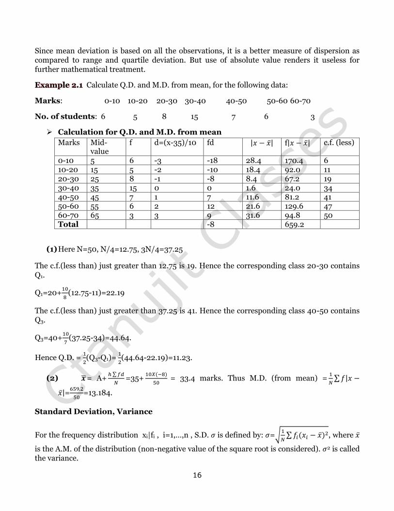
16
Since mean deviation is based on all the observations, it is a better measure of dispersion as compared to range and quartile deviation. But use of absolute value renders it useless for further mathematical treatment.
Calculate Q.D. and M.D. from mean, for the following data:
Marks: 0-10 10-20 20-30 30-40 40-50 50-60 60-70
No. of students: 6 5 8 15 7 6 3
Calculation for Q.D. and M.D. from mean
Marks Mid-value
f d=(x-35)/10 fd | | f| | c.f. (less)
0-10 5 6 -3 -18 28.4 170.4 6 10-20 15 5 -2 -10 18.4 92.0 11 20-30 25 8 -1 -8 8.4 67.2 19 30-40 35 15 0 0 1.6 24.0 34 40-50 45 7 1 7 11.6 81.2 41 50-60 55 6 2 12 21.6 129.6 47 60-70 65 3 3 9 31.6 94.8 50 Total -8 659.2
(1) Here N=50, N/4=12.75, 3N/4=37.25
The c.f.(less than) just greater than 12.75 is 19. Hence the corresponding class 20-30 contains Q1.
Q1=20+
(12.75-11)=22.19
The c.f.(less than) just greater than 37.25 is 41. Hence the corresponding class 40-50 contains Q3.
Q3=40+
(37.25-34)=44.64.
Hence Q.D. =
(Q3-Q1)=
(44.64-22.19)=11.23.
(2) = A+ ∑
=35+
= 33.4 marks. Thus M.D. (from mean) =
∑ |
|=
=13.184.
Standard Deviation, Variance
For the frequency distribution xi|fi , i=1,…,n , S.D. is defined by: =√
∑ , where
is the A.M. of the distribution (non-negative value of the square root is considered). 2 is called the variance.
17
Note s2=
∑ =
∑ =
∑ +( -A)2+2( -A)(xi- )}
=
∑ +( -A)2
∑ +2( -A)
∑ = 2+( -A)2, where d= -A.
Thus s2 is least when d=0.that is, when =A. Thus M.D. is least when A= and S.D. is least value of M.D.
Note (1) 2=
∑ =
∑
) =
∑
+
∑ -
2
∑ =
∑
+ -2 =
∑
(
∑ )
. This expression is often used for
calculation of 2.
(2)If n1 and n2 are the sizes, and be the means and 1 and 2 be the S.D. s of two
series, then the S.D. of the combined series of n1+n2 observations is given by:
2=
[
)+
)], where d1= - , d2= - and =
is the mean of
the combined series.
For a group of 200 candidates , the mean and S.D. of scores were found to be 40 and 15 respectively. Later on it was discovered that the scores 43 and 35 were misread as 34 and 53 respectively. Find the corrected mean and S.D. corresponding to the corrected figures.
Let x be the given variable. Given n=200, =40 and =15. Now 40= =
∑ gives
∑ =8000.
2=
∑
- 2 gives ∑ =200(225+1600)=365000.
Corrected ∑ =8000-34-53+43+35=7991, corrected mean =
=39.995
Corrected ∑ = 365000-342-532+432+352=364109
Corrected 2=
(39.995)2=224.14. Thus corrected =√ =14.97.
The first of two samples has 100 items with mean 15 and s.d. 3.if the whole
group has 250 items with mean 15.6 and s.d. √ . find s.d. of the second group.
Here n1=100, =15, 1=3, n=n1+n2=250, =15.6, =√
=
gives =16. Hence d1= - =15-15.6=-0.6, d2= - =16-15.6=0.4
From 2=
[
)+
)], 2=4.
Moments
The r th (raw) moment of a variable x about any point A , denoted by
, is given by
=
∑ .
18
The r th (central) moment of a variable x about mean , denoted by , is given by
=
∑ .
In particular, =
∑ =
∑ =1, =
∑ =0, =
∑ = 2.
Relation between raw and central moments
=
∑ =
∑ =
∑ , where di=xi-A.
=A+
∑ =A+
. Hence =
∑
=
∑
+
-…+(-
1)r )
= -
+
-…+(-1)r
.
In particular, on putting r=2,3,4 and simplifying, we get = /-
, =
/-3 /
/+2
,
=
+6
-3
.
Effect of change of origin and scale on Moments
Let u=
. Then . Thus x- =h(u- ). Thus =
∑
∑
hr .
Symmetrical and Skew Distributions
A distribution is symmetrical when the frequencies are symmetrically distributed about the mean , that is, when the values of the variate equidistant from mean have equal frequencies. For example, the following distribution is symmetrical about its mean 5:
x: 1 2 3 4 5 6 7 8 9
f: 3 4 6 9 10 9 6 4 3
It can be seen that if n is odd,
∑
=0 since all the terms cancel in pairs, n being odd
and f1=fn, f2=fn-1,…. Thus =0 , for n odd. Hence for a symmetrical distribution,
= 0.
Thus is a measure of departure from symmetry.
Also for a symmetrical distribution, the mean, median and mode coincide. Further, in the case of such distribution, median lies halfway between the two quartiles.
Skewness means lack in symmetry. It indicates whether the frequency curve is inclined more to one side than the other, that is , whether the frequency curve has a longer tail on one side. Skewness is positive if the curve is more elongated to the right side, that is, if the mean of the distribution is greater than the mode; in the reverse case, it is negative. Skewness gives an
19
idea about the direction in which also the extent to which the distribution is distorted from the symmetrical distribution.
For distribution of moderate skewness, an empirical relation holds: mean-mode= 3(mean-median).
Karl Pearson’s coefficient of skewness is given by : coefficient of
skewness=
=
.
It is a pure number since the numerator and denominator have the same dimension. It has value zero for a symmetrical distribution.
Bowley’s measure of skewness is
.
Find out a coefficient of dispersion based on quartile deviation and a measure of skewness from the following table giving wages of 230 persons:
Wages(in Rs) f c.f. Wages(in Rs) f c.f.
140-160 12 12 220-240 50 157
160-180 18 30 240-260 45 202
180-200 35 65 260-280 20 222
200-220 42 107 280-300 8 230
Here N/2=115 and the 115 person has a wage in the class 220-240. Hence median=Q2=
220+
x 20 = Rs. 223.20. Similarly, Q1=180+
x 20=Rs. 195.71,
Q3=240+
x 20=Rs. 246.88. It can be shown that mean=Rs. 220.87, S.D.= Rs.
34.52.
Coefficient of dispersion based on quartile deviation=
=
=0.1156.
Measure of skewness =
=
= - 0.3514
Second measure of skewness=
=- 0.07446.
Pearson’s and - Coeficients
, √ ,
, = -3.
The values of the two coefficients , enable us to know whether the given distribution is
symmetrical and whether it is relatively more or less flat than the normal curve. gives a measure of departure from symmetry. Kurtosis measures whether the given frequency curve is relatively more or less flat –topped compared to the normal curve (to be studied later). For a
normal distribution , =3. Curves with values of less than 3 are called Platykurtic whereas
20
those with values of greater than 3 are called Lettokurtic. Curves with value equal to 3 are called Mesokurtic.
BASIC PROBABILITY THEORY
Basic Terminology
Random Experiment : If in each trial(repetition) of an experiment conducted under identical conditions, the outcome is not unique , but may be any one of possible outcomes, then such an experiment is called a random experiment. Examples of random experiments are: tossing a coin, throwing a die, selecting a card from a pack of playing cards etc. in all these cases, there are a number of possible outcomes which can occur but there is an uncertainty as to which of them will actually occur.
A piece of Information: A pack of cards consists of four suits called Spades, Hearts and Clubs. Each suit consists of 13 cards, of which nine cards are numbered from 2 to 10, an ace, a king, a queen and a jack(or knave).Spades and clubs are black-faced cards while hearts and diamonds are red-faced cards.
Outcome: result of a random experiment is called an outcome.
Sample Space, Events: The collection S of all possible outcomes of a random experimepernt is called sample space of the random experiment; any subset of S is an event; a singleton subset of S is an elementary(simple) event. For example, in an experiment which consists of throwing a six-faced die, possible outcomes are 1,2,3,4,5,6. Thus sample space of this experiment is {1,2,3,4,5,6}, {1} is an elementary event; getting an even number, {2,4,6} is an event of this experiment.
Exhaustive Events: events E1,…,Ek of a random experiment with sample space S are called
exhaustive iff S = E1 Ek. in the case of throwing of a die, getting even points( that is, 2,4, or 6) and getting odd points (that is, 1,3, or 5) are exhaustive events.
Equally Likely Events: Events are equally likely if there is no reason to expect any one of them compared to others. In the trial of drawing a card from a well-shuffled pack of cards, any of the 52 cards may appear, so that the 52 elementary events are equally likely.
Exclusive Events: Events are exclusive if the occurrence of any one of them precludes the occurrence of all others. On the contrary, events are compatible if it is possible for them to happen simultaneously. For instance, in the rolling of two dice, the cases of the face marked 5 appearing on both dice are compatible.
Favourable Events: The trials which entail the happening of an event are favourable to the event. For example, in the tossing of a dice, the number of favourable events to the appearance of a multiple of 3 are two viz. getting 3 and 6.
21
Classical (a priori) definition of probability
If a random trial results in n exhaustive, mutually exclusive and equally likely outcomes, out of which m are favourable to the occurrence of an event E, then the probability of occurrence of E
, denoted by P(E), is given by P(E)=
.
It is clear from definition that 0 p 1. Since the number of cases in which event A will not
happen is n-m, the probability q that the event A will not happen is given by P =
=1-
=1-
P(A).
An event A is certain to happen if all the trials are favourable to it and then the probability of its happening is unity; for an event which is certain not to happen, the probability is zero.
Find the chance that if a card is drawn at random from an ordinary pack, it is one of the court cards.
Court cards are kings, queens, jacks and their number in a pack of 52 cards is 12, so that
the number of favourable events is 12. Hence the probability is 12/52=3/13.
What is the chance that a leap year selected at random will contain 53 Sundays?
A leap year which contains 366 days has 52 Sundays corresponding to 52 weeks and 2
more days.There are following seven possibilities: (1) Sunday, Monday, (2)
Monday,Tuesday,(3) Tuesday, Wednesday, (4) Wednesday, Thursday, (5) Thursday,
Friday, (6) Friday , Saturday, (7) Saturday, Sunday. Out of these seven possibilities,
there are two favourable outcomes, namely (1) and (8). Thus the required probability is
2/7.
An urn contains 9 balls, two of which are red, three blue and four black.Three balls are drawn from the urn at random. What is the chance that (1) three balls are of different colours, (2) two balls are of the same colour and third is different, (3) the balls are of the same colour?
(1) Three balls can be drawn from 9 balls in =84 ways and these are equally likely,
exhaustive and mutually likely cases. A red ball can be drawn in 2 ways, a blue in 3 and a
black in 4 ways, so that three differently coloured balls can be drawn in 2 x 3x 4=24
ways. Hence the probability is 24/84=2/7.
(2)two blue balls can be drawn in ways and then a red or black ball in 6 ways so that
the two blue balls and a different coloured ball can be drawn in 6x =18 ways. Two
black balls and a different coloured ball can be drawn in 5x =30 ways. Similarly the
number of ways in which two red balls and a different coloured ball can be drawn in
7x =7 ways. Thus the number of ways two balls of same colour and a ball of different
colour can be drawn is 18+30+7=55. Thus required probability is 55/84.
22
(3)Three blue balls can be drawn in 1 way and 3 black balls in or 4 ways so that the
corresponding probability is 5/84.
Limitation of Classical Definition
This definition breaks down in the following cases:
If the various outcomes of the random experiment are not equally likely
If the number of exhaustive outcomes of the random experiment is infinite or unknown
Von Mises’s statistical (or empirical) definition of probability
If trials be repeated a great number of times under essentially same conditions, then the limit of the ratio of the number of times that an event happens to the total number of trials, as the number of trials increases indefinitely, is the probability of the happening of the event,provided the ratio approaches a finite and a unique limit.
Axiomatic definition of Probability
To an event A(that is, a subset of sample space S) is assigned a real number P(A), called probability of A, satisfying the following properties:
(Axiom of non-negativity)P(A) 0
(Axiom of certainty) P(S)=1
(Axiom of Additivity) If {An} is any finite or infinite sequence of disjoint events, then
P ⋃ ∑
.
Note P, the probability function, is otherwise unspecified except it is to satisfy above three axioms.
Notation for two events A,B of a sample space S,A B={x S: x A or x B}, A B={x S: x A
and x B}, = { x S: x∉A}, A-B={ x S: x and x∉B}, A B can be denoted by A+B, if A and B
are disjoint; A B=( B)+(A ).
Let A,B,C are three arbitrary events. Find expression for the following events:
(1)Only A occurs, (2) Both A,B but not C , occur, (3) All three events occur, (4) At least one occurs, (5) At least two occur, (6) one and no more occurs, (7) two and no more occur, (8) none occurs.
(1) A , (2) A , (3) A , (4)A , (5) (A ) A
), (6) ( ) ( ) ( ), (7) )
) ), (8) .
Some Theorems on Probability
Theorem3.1 Probability of impossible event is zero: P( )=0.
23
S=S and S, are disjoint events. Using axiom of additivity, P(S)=P(S
)=P(S)+P( ); hence P( )=0.
: P(A)=0 does not necessarily mean A is impossible event. In case of continuous random variable X, the probability at a point is always zero: P(X=c)=0.
Theorem3.2 P( =1-P(A).
1=P(S)=P(A )=P(A)+P( (since A = ).
Corollary 0 P( =1-P(A); hence 0 P(A) 1.
Lemma For two events A,B, P(
and are disjoint events and B=B =B (A )=( )
; hence by axiom of additivity, P( .
Corollary (1) If A B, then P( P(B)-P(A), (2) P(A) P(B).
Theorem3.3 (Addition Theorem of Probability) If A,B are any two events,
P(A B)=P(A)+P(B)-P( ).
A B=A ( ) and A, are disjoint. Hence P(A B)=P(A)+ P( = P(A)+P(B)-
P( ).
Generalising , for three events A,B,C, we have
P( .
If p1=P(A), p2=P(B), p3=P( ), express the following in terms of p1,p2,p3: (1)
P( ), (2) P( , (3)P( B),(4) P(
(1) P( )=1-P(A =1-[P(A)+P(B)-P(A B)]=1-p1-p2-p3.(2) P( )=P( )=1-
P( B)=1-p3. (3) P( B)=P(B)- P( B)=p2-p3.(4) P( )=P( )+P(B)- P( B)=1-
p1+p2-( p2-p3)=1-p1+p3.
It two dice are thrown, what is the probability that the sum is (1) greater than 8, (2)neither 7 nor 11?
(1)If X denotes the sum on the two dice, then we want P(X>8). The required event can
happen in the following mutually exclusive cases: X=9, X=10,X=11,X=12. Hence by
addition theorem on probability, P(X>8)=P(X=9)+P(X=10)+P(X=11)+P(X=12). In a
throw of two dice, the sample space contains 62=36 points. The number of favourable
cases can be enumerated as:
X=9: (3,6),(6,3),(4,5),(5,4) X=10: (4,6),(6,4),(5,5) X=11: (5,6),(6,5)
24
X=12:(6,6).
Thus P(X>8)=
=
.
(2)Let A denote the event of getting the sum of 7 and B denote the event of getting the sum of 11 with a pair of dice. X=7: (1,6),(6,1),(2,5),(5,2),(3,4),(4,3) X=11: (5,6),(6,5)
Required probability= P( )=1-P(A B)=1-[P(A)+P(B)] (since A and B are disjoint
events)=1-
=
.
Two dice are tossed. Find the probability of getting an even number on the first die or a total of 8.
Let A be the event of getting an even number on the first dice and B be the event that the
sum of points obtained on the two dice is 8. The events are represented by the following
subsets of the sample space S:
A={2,4,6} X {1,2,3,4,5,6}, B={(2,6),(6,2),(3,5),(5,3),(4,4)}. Here A B={(2,6),(6,2),4,4)}.
Required probability is P(A B)=P(A)+P(B)-P(A B)=
=
.
An integer is chosen at random from first two hundred natural numbers. What is the probability that the integer is divisible by 6 or 8?
Sample space of the random experiment is {1,2,…,200}. The event A ‘ integer chosen is
divisible by 6’ is given by {6,12,…,198}; the event B‘ integer chosen is divisible by 8’ is
given by {8,16,…,200}. LCM of 6 and 8 is 24. Hence a number is divisible by 6 and 8 iff
it is divisible by 24. Thus A B={24,48,…,192}. Hence required probability is
P(A B)=P(A)+P(B)-P(A B)=
=
.
The probability that a student passes Physics test is 2/3 and the probability that he passes both Physics test and English test is 14/45.The probability that he passes at least one test is 4/5. What is the probability that he passes English test?
Let A be the event that the student passes the Physics test and B be the event that he
passes English test. Given P(A)=
, P(A B)=
, P(A B)=
. We want P(B). From
P(A B)=P(A)+P(B)-P(A B), we get P(B)=
.
An investment consultant predicts that the odds against the price of a certain stock will go up during the next week are 2:1 and the odds in favour of the price remaining the same are 1:3.What is the probability that the price of the stock will go down during the next week?
25
Let A denote the event ‘ stock price will go up’ and B be the event ‘stock price will remain
same’. Then P(A)=
, P(B)=
. Thus P(A B)=P(A)+P(B)=
. Hence the
probability that the stock price will go down is given by P( )=1- P(A B)=1-
=
.
An MBA applies for a job in two firms X and Y. The probability of his being selected in firm X is 0.7 and being rejected at Y is 0.5. The probability of at least one of his applications being rejected is 0.6. What is the probability that he will be selected in one of his firms?
Let A and B denote the events that the person is selected in firms X and Y respectively.
Then P(A)=0.7, P =0.5. Thus P =1-0.7=0.3, P(B)=1-0.5=0.5 and 0.6= P( )=
P + P P( ). The probability that the person will be selected in one of the
twofirms X or Y is given by: P(A B)=1- P( )=1-[ P P P( ]=1-
(0.3+0.5-0.6)=0.8.
Three newspapers A,B and C are published in a certain city. It is estimated from a survey that 20% read A, 16% read B, 14% read C, 8% read both A and B, 5% read both A and C, 4% read both B and C, 2% read all three. Find what percentage read at least one of the papers?
Let E,F,G denote the events that a person reads newspapers A,B and C respectively.
Then we are given: P(E)=
, P(F)=
, P(G)=
, P(E F)=
, P(E G)=
,
P(G F)=
, P )=
.
The required probability that a person reads at least one of the newspapers is given by
P )=P(E)+P(F)+P(G)- P(E F)- P(E G)- P(G F)+ P )=
=0.35.
A card is drawn from a pack of 52 cards. Find the probability of getting a king or a heart or a red card.
Let A,B and C denote the event ‘card drawn is a king’, ‘card drawn is a heart’ and ‘card
drawn is a red card’ respectively. Then A,B,C are not mutually exclusive.
A B: card drawn is king of hearts ; n(A B)=1
B =B( since B C): card drawn is a heart ;n(B )=13
A : card drawn is a red king; n(A )=2
A = A : card drawn is the king of hearts; n(A )=1.
Thus P(A)=
, P(B)=
, P(C)=
, P(A B)=
, P(B )=
, P(A )=
, P(A
)=
. Thus required probability is P( )=P(A)+P(B)+P(C)- P(A B)- P(B )-
P(A )+ P(A )=
.
26
Conditional Probability
In many situations we have the information about the occurance of an event A and are required to find out the probability of the occurrence of another event B. This is denoted by P(B/A). For example, if we know that a card drawn from a pack is black, we may need to calculate the probability that it is the ace of spade.
Let us take the problem of throwing a fair die twice. Suppose same number of spots do not appear in both the throws and we are required to find the probability that the sum of number of spots in the two throws is six.
A patient comes to a doctor with his family history that his elders suffered from high blood pressure. He wants to know the probability of the event that he will also suffer from high blood pressure.
Definition Let A and B be two events. The conditional probability of event B supposing
event A has occurred, is defined by P(B/A)=
, if P(A)>0.
Note Let B1,…,Bk be mutually exclusive events. The conditional probability of ⋃ given that
event A has occurred is given by P(⋃
)
[(⋃ ) ]
=
∑
.
If a card drawn from a pack is black, represented by event A, find the probability of the event B that the card drawn is ace of spade .
Number of black cards in a pack of 52 cards is 26. P(A)=26/52=1/2. Out of 26 black
cards, only one is ace of spade. The event A B contains only one point; thus
. Hence P(B/A)=
=
=
.
An experiment is conducted by throwing a fair dice twice. Let A be the event that same number of spots do not turn up in two throws and B be the event that sum of the spots is 6. Find P(B/A).
A includes all 36 points of the sample space except (1,1),(2,2),(3,3),(4,4),(5,5) and (6,6).
Thus P(A)=30/36=5/6. Points favourable to event B are (1,5),(2,4),(3,3),(4,2),(5,1).
Points common to A and B , that is A B , are (1,5),(2,4),(4,2),(5,1). Thus P(A B)=4/36.
Thus P(B/A)=
=
=0.133.
10% of patients feel they suffer and are really suffering from TB, 30% feel they suffer but actually do not suffer, 25% do not feel they are suffering but are suffering and remaining 35% neither feel nor suffering from TB. Find the probility of events E1,E2,E3,E4, where E1: person who suffers from TB and feels he suffering from TB, E2: person has TB and does not feel, E3:person feels he has TB and does not suffer from TB, E4: person feels and has TB.
27
Let us define events: A: person feels he has TB, B: person suffers from TB. P(A B)=0.1,
P(A =.3, P( B)=.25, P( )=.35. Thus P(A)= P(A B)+ P(A =0.1+0.3=0.4,
P(B)= P(A B)+ P( B)=.10+.25=.35, P( )= P( B)+P( )=0.25+0.35=0.6,P( )=
P(A )+ P( )=0.3+0.35=0.65. Hence
P(E1)=P(B/A)=
, P(E2)=P(B/ )=
=0.417,P(E3)= P(A/ )=0.462,
P(E4)=P(A/B) = 0.286.
There are two lots of manufactured item. Let one contain 40 pieces whereas lot two contains 50 pieces.it is known that former lot contains 25% defective pieces and the later one 10%. We flip a coin and select a piece from a lot one if it turns with head up; otherwise we select a piece from lot 2. Find the probability that a selected piece will be defective.
Let A,B stand for the event ‘piece is selected from lot 1’ and ‘piece is selected from lot 2’.
Since the probability of turning head up=1/2, we have P(A)=1/2 and P( )=1/2. Lot 1 has
10 defective and 30 non-defective pieces; lot 2 has 5 defective and 45 non-defective
pieces. Given P(B/A)=1/4, P(B/ =1/10. Thus P(A B)=P(B/A)P(A)=1/8, P( B)=
P(B/ P( )=1/20. Hence the probability that the selected item is defective is P(A B)+
P( B)=0.175.
Independent Events
If we draw two cards from a pack of cards in succession, then the results of the two draws are independent if the cards are drawn with replacement and are not independent if the cards are drawn without replacement.
Definition An event A is independent of another event B iff P(A/B)=P(A). This definition is
meaningful when P(A/B) is defined, that is, when P(B) 0.
Theorem3.4 If two events A and B are such that P(A) 0, P(B) 0 and A is independent of B, then B is independent of A.
P(A/B)=P(A)⇒
⇒ =P(A)P(B) ⇒P(B/A)=
=
=P(B).
Theorem3.5 If A,B are events with positive probilities, then A and B are independent iff
=P(A)P(B).
Theorem3.6 If A and B are independent, then (1) A and , (2) and B , (3) , are independent.
Since A and B are independent, =P(A)P(B). P(A )=P(A)- =P(A)-
P(A)P(B)=P(A)P( ). P( )=P( )=1-P(A B)=1-[P(A)+P(B)- )]=1-P(A)-
P(B)+P(A)P(B)=[1-P(A)][1-P(B)]=P( )P( ).
28
If , then show that P(A) P(
A=( )= )= ⇒A ⇒ P(A) P( .
Let A and B be two events such that P(A)=3/4, P(B)=5/8. Show that (a)
P(A B)
, (b)
.
(a) A A ⇒
.
(b) B⇒P( P(B)=
. Also, B) ⇒
) ⇒
BAYES’ THEOREM
Theorem3.7 If E1,E2,…,En are mutually disjoint events with P(Ei) 0(i=1,…,n), then for any
arbitrary event A which is a subset of ⋃ such that P(A)>0,
P(Ei/A)=
∑
Suppose that a product is produced in three factories X,Y, and Z. It is known that factory X produces thrice as many items as factory Y and that factory Y and Z produces same number of items. 3% of the items produced by each of the factories X and Z are defective and 5% of those manufactured in Y are defective. All the items in the three factories are stocked and an item of the product is selected at random. (1) What is the probability that the item selected is defective? (2) if an item selected at random is found to be defective, what is the probability that it was produced in factory X,Y,Z respectively?
Let the number of items produced by factories X,Y, and Z be 3n,n,n respectively. Let
E1,E2,E3 be the events that the items are produced by factory X,Y and Z respectively and
let A be the event that the item being defective. Then P(E1)=
=0.6, P(E2)=0.2,
P(E3)=0.2. Also, P(A/E1)= P(A/E3)=0.03, P(A/E2)=0.05(given).
(1) The probability that an item selected at random from the stock is defective is given
by P(A)=∑ ∑
=.6 x .03+.2x.05+.2x.03=.034.
(2) By Bayes’ rule, the required probabilities are given by :
P(E1/A)=
=
, P(E2/A)=
=
, P(E3/A)=
.
In 2002 there will be three candidates for the position of the principal –Mr. x, Mr. y and Mr.z—whose chances of getting the appointment are in the ratio 4:2:3 respectively. The probability that Mr. x if selected would introduce co-education in the college is 0.3. The corresponding probabilities for Mr. y and Mr.z are 0.5 and 0.8. (1) What is the probability that there will be co-education in 2003? (2) if there is co-education in 2003, what is the probability that Mr. z is the principal?
29
Let us define the events
A: introduction of co-education, E1: Mr. x is selected as principal
E2: Mr. y is selected as principal, E3: Mr. z is selected as principal.
P(E1)=4/9, P(E2)=2/9, P(E3)=3/9, P(A/E1)=3/10, P(A/E2)=5/10, P(A/E3)=8/10.
(1) The required probability that there will be coeducation in the college in 2003 is
P(A)=P[(A E1) ]= P(A E1)+ P(A E2)+ P(A E3)
=P(E1)P(A/E1)+ P(E2)P(A/E2)+ P(E3)P(A/E3)=
=
.
(2) The required probability is given by Bayes’ rule:
P(E3/A)=
=
=
.
RANDOM VARIABLES
In many random experiments, we are interested not in knowing which of the outcomes has occurred but in the numbers associated with them. For example, when n coins are tossed, one may be interested in knowing the number of heads obtained. When a pair of dice are tossed, one may seek information about the sum of points. Thus, we associate a real number with each outcome of a random experiment. In other words, we are considering a function whose domain is the set of all possible outcomes and whose range is a subset of the set of reals.
Definition Let S be the sample space associated with a given random experiment. A real-
valued function X: S ) is called a one-dimensional random variable(r.v.).
Notation If x is a real number, the set of all w S such that X(w)=x is denoted by X=x. Thus
P(X=x)=P{w: X(w)=x}. Similarly P(X a)= P{w ] },
P(a<X b)=P{w:X(w) (a,b]}
Consider the random experiment of tossing a coin. Then S={w1,w2}, w1=H,w2=T.
Define X:{w1,w2} {0,1} by X(w1)=1, X(w2)=0. X is a r.v.
A function X:S→R2 is a two-dimensional random variable.
: If a dart is thrown at a circular target, the sample space S is the set of all points w on the target.By imagining a co-ordinate system placed on the target with the origin at the centre, we can consider a two-dimensional random variable X which assigns to every point w of the circular region , its rectangular co-ordinates (x,y)
If a pair of dice is tossed , then S={1,2,3,4,5,6}X{1,2,3,4,5,6} .Let X be the random variable defined by X(i,j)=max{i,j}. Then
P(X=1)=P{(i,j):X(i,j)=1}=P{(1,1)}=1/36, P(X=2)=P{(1,2),(2,2),(2,1)}=3/36.
30
Distribution Function
Definition Let X be a random variable(r.v.). The function F : (-∞,∞)→[0,1] defined by F(x)=P{t: X(t)≤x} is the distribution function (d.f.) of the r.v. X.
Note: To emphasize the r.v. X, we sometimes denote F(x) by FX(x).
Properties of Distribution Function
(1) If F is the d.f. of the r.v. X and if a<b, then P(a<X≤b)=F(b)-F(a).
The events a<X≤b’ and X≤a are disjoint and their union is the event X≤b. Hence,
by addition theorem of probability,
P(a<X≤b)+P(X≤a)=P(X≤b). Hence the result.
Corollary: P(a≤X≤b)=P{(X=a) (a<X≤b)}=P(X=a)+ P(a<X≤b) =
P(X=a)+ [F(b)-F(a)]. When P(X=a)=0, the events
a≤X≤b and a<X≤b have same probability F(b)-F(a)
(2) 0≤F(x) ≤1. If x<y, then F(x) ≤F(y).
Discrete Random Variable
A r.v. which can assume only at most countable number of real values is a discrete random variable. Example of discrete random variable are marks obtained in a test, number of accidents per month etc.
Probability Mass Function
If X is a one-dimensional discrete r.v. taking at most a countable number of values x1,x2,…, then the probabilistic behaviour of X at each xi is described by its probability mass function.
Definition If X is a discrete r.v. having distinct values x1,x2,…, then the function pX(x), or simply p(x), defined by p(x)=P(X=xi)=pi, if x=xi and =0, if x≠xi, i=1,2,… is called probability mass function(p.m.f.) of r.v. X.
Note (1)The set {(x1,p1),(x2,p2),…} specifies the probability distribution of the r.v. X.
(2)P(xi)≥0 , for all i and ∑
Let S={H,T} be the sample space corresponding to the random experiment of tossing of a ‘fair’ coin. Let X be the r.v. defined by X(H)=1, X(T)=0. X has only two distinct values, namely, 0 and 1. The corresponding p.m.f. is given by: p(1)=P(X=1)=P(H)=1/2, p(0)=1/2.
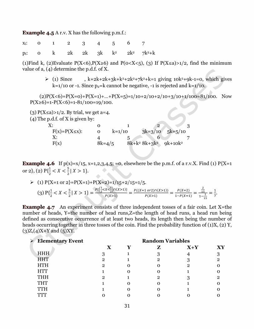
31
A r.v. X has the following p.m.f.:
xi: 0 1 2 3 4 5 6 7
pi: 0 k 2k 2k 3k k2 2k2 7k2+k
(1)Find k, (2)Evaluate P(X<6),P(X≥6) and P(0<X<5), (3) If P(X≤a)>1/2, find the minimum value of a, (4) determine the p.d.f. of X.
(1) Since , k+2k+2k+3k+k2+2k2+7k2+k=1 giving 10k2+9k-1=0, which gives
k=1/10 or -1. Since p2=k cannot be negative, -1 is rejected and k=1/10.
(2)P(X<6)=P(X=0)+P(X=1)+…+P(X=5)=1/10+2/10+2/10+3/10+1/100=81/100. Now P(X≥6)=1-P(X<6)=1-81/100=19/100.
(3) P(X≤a)>1/2. By trial, we get a=4.
(4) The p.d.f. of X is given by:
X: 0 1 2 3 F(x)=P(X≤x): 0 k=1/10 3k=3/10 5k=5/10
X: 4 5 6 7 F(x) 8k=4/5 8k+k2 8k+3k2 9k+10k2
If p(x)=x/15, x=1,2,3,4,5; =0, elsewhere be the p.m.f. of a r.v.X. Find (1) P{X=1
or 2}, (2) P{
| .
(1) P{X=1 or 2}=P(X=1)+P(X=2)=1/15+2/15=1/5.
(3) P{
|
(
)
.
An experiment consists of three independent tosses of a fair coin. Let X=the number of heads, Y=the number of head runs,Z=the length of head runs, a head run being defined as consecutive occurrence of at least two heads, its length then being the number of heads occurring together in three tosses of the coin. Find the probability function of (1)X, (2) Y, (3)Z,(4)X+Y and (5)XY.
Elementary Event Random Variables
X Y Z X+Y XY HHH 3 1 3 4 3 HHT 2 1 2 3 2 HTH 2 0 0 2 0 HTT 1 0 0 1 0 THH 2 1 2 3 2 THT 1 0 0 1 0 TTH 1 0 0 1 0 TTT 0 0 0 0 0
32
(1)Obviously X is a r.v. which can take the values 0,1,2, and 3. p(3)=P(HHH)=(
)
=
,
p(2)=P(HHT )=P(HHT)=P(HTH)+P(THH)=1/8+1/8+1/8=3/8. Similarly p(1)=3/8, p(0)=1/8.
(2) probability distribution of Y: p(0)=5/8, p(1)=3/8.
(3)probability distribution of Z: p(0)=5/8, p(1)=0,p(2)=2/8,p(3)=1/8.
(4) probability distribution of U=X+Y:p(0)=1/8, p(1)=3/8,p(2)=1/8,p(3)=2/8,p(4)=1/8.
(5) probability distribution of V=XY: p(0)=5/8,p91)=0,p(2)=2/8,p(3)=1/8.
Continuous Random Variable
Definition A r.v. X is continuous iff X takes all values between two unequal real numbers.
Probability Density Function
Consider a small interval (x, x+dx) of length dx about x. Let f(x) be any continuous function of x so that f(x)dx represents the probability that X falls in the infinitesimal interval (x, x+dx).
Symbolically, P(x =fX(x)dx. fX is called probability density function (p.d.f.) of the r.v. X.
The probability for a variate value to lie in the interval [a,b] is P(a X b)=∫
.
The p.d.f. f(x) of a r.v. X has the properties:
f(x) 0, ∫
=1 (since ∫
gives total probability), P(X=c)= ∫
=0(where c
is any value of the variate X)
Various measures of central tendency, dispersion, skewness and kurtosis for continuous probability distribution
The formulae for these measures in case of discrete frequency distribution can be easily extended to the case of continuous probability distribution by simply replacing pi=fi/N by f(x)dx, xi by x and summation over ‘i’ by integration over the specified range of the variable X.
Let f(x) be the p.d.f. of a r.v. X, [a,b] being the range of X. Then
A.M. =∫
, (central)=∫
,
(about x=A)=∫
Median is the point which divides the total area into two equal parts: if M be the median, then
∫ ∫
Mode is the value of x for whixh f(x) is maximum. Mode is the solution of f/(x)=0 and f//(x)<0, provided it lies in [a,b].
33
The diameter of an electric cable , say X, is assumed to be a continuous
random variable with p.d.f. f(x)=6x(1-x), 0 x 1. (1) Check that f(x) is a p.d.f., (2) determine the median b of the distribution.
(1) ∫
(by direct calculation); hence f(x) is p.d.f. of r.v. X. (2)
P(X<b)=P(X>b)⇒ ∫
∫
⇒ b=1/2, lying in [0,1].
Suppose that the life in hours of a certain part of radio tube is a continuous
random variable X with p.d.f. given by f(x)=100/x2, when x 100; =0, elsewhere. (1) What is the probability that all of three such tubes in a given radio set will have to be replaced during the first 150 hours of operation?(2)What is the probability that none of the original tubes will have to be replaced during the first 150 hours of operation?(3)what is the probability that a tube will last less than 200 hours if it is known that the tube is still functioning after 150 hours of service?
(1)p=P(X 150)=∫ ∫
. By compound probability theorem, the
probability that all three of original tubes will have to be replaced during the first 150
hours =p3=1/27.
(2)The probability that a tube is not replaced during the first 150 hours of operation is
P(X>150)=1-P(X 150)=1-p=2/3. By compound probability theorem, the probability that none of the three tubes will have to be replaced during the first 150 hours =q3=8/27. (3)Probability that a tube will last less than 200 hours given that the tube is still
functioning after 150 hours is P(X<200|X>150)=
=
∫
∫
=0.25.
The amount of bread (in hundreds of pounds) x that a certain bakery is able to sell in a day is found to be a numerical valued random phenomenon with a probability
function specified by the p.d.f. f(x) given by f(x)=kx, 0 x<5; =k(10-x), 5 x<10; =0, otherwise. (1) find the value of k such that f(x) is a p.d.f., (2)what is the probability that the number of pounds of bread that will be sold tomorrow is (a) more than 500 pounds, (b) less than 500 pounds and (c) between 250 and 750 pounds? (3) Denoting by A,B,C the events that the pounds of bread sold are as in (2)(a),(2)(b) and (2)(c) respectively, find P(A|B),P(A|C). Are (1) A,B independent, (2) A,C independent?
(1)∫
=1 gives k=1/25.
(2)(a)P(5 10)=∫
=0.5
(b)P(0 ∫
0.5
(c)P(2.5 ∫
∫
=3/4
(3)From (2)(a),(b),(c), P(A)=0.5, P(B)=0.5, P(C)=3/4. The events A B and A are
given by: A B= , A :5<X<7.5. Thus P(A B)=0,P(A C)=
∫
=3/8.
34
P(A)P(C)=1/2 X ¾=3/8=P(A ), P(A)P(B)=1/4 P(A B). Thus A,C are independent and A,B are not independent.
Expectation of a r.v.
Let the r.v. X take values x1,…,xn with probabilities p1,…,pn. Let X take value xi , fi number of
times; let N=f1+…+fn. Mean of X is given by
. Let N . Using the
statistical definition of probability, limiting value of mean of X , .
Definition Expectation of X, E(X)=∑ .
Thus E(X) may be regarded as the limiting value of the average value of X realized in N random
experiments as N . Generalising, if f(X) is a function of X, f(X) will take values f(x1),…,f(xn)
with frequencies f1,…,fn and the average value of f(X) in N experiments is
f(x1)+…+
f(xn) and
as N , this approaches to E(f(X))=p1f(x1)+…+pnf(xn). In particular, =E[(X-a)r],
[ r], [ 2]= .
What is the expectation of the number of failures preceding the first success in an infinite series of independent trials with constant probability p of success in a trial?
If X denotes the number of failures preceding the first success , we find that X takes the
values 0,1,2,3,… with probabilities p,qp,q2p,q3p,…, where q=1-p. Thus probability
density function is f(x)=qrp, r=0,1,2,…. Hence
E(X)=0.p+1.qp+2.q2p+3.q3p+…=pq(1+2q+3q2+…)=pq(1-q)-2 (since q<1)=q/p = 1/p-1.
Properties of Expectation
1. Addition Theorem of Expectation: If X,Y are r.v., then E(X+Y)=E(X)+E(Y).
2. Multiplication Theorem of Expectation: If X,Y are independent r.v., E(XY)=E(X)E(Y).
3. If X is a r.v. and a,b are constants, then E(aX+b)=aE(X)+b, provided all the expectations
exist.
4. If X 0,then E(X) 0.
5. If X,Y are r.v. and X(t) Y(t), forall t, then E(X) E(Y), provided all expectations exist.
Let X be a r.v. with the following probability distribution:
x: -3 6 9
P(X=x): 1/6 ½ 1/3
Find E(X) and E(X2) and using laws of expectation, evaluate E(2X+1)2.
E(X)=∑ =(-3)
=
, E(X2)=∑
. Then
E(2X+1)2=4E(X2)+4E(X)+1=209.

35
Two unbiased dice are thrown. Find the expected values of the sum of numbers of points on them.
The probability function of X(sum of number of heads on two dice) is
x: 2 3 4 … 12 P(X=x): 1/36 2/36 3/36 … 1/36
E(X)=∑
=7.
SOME IMPORTANT DISTRIBUTIONS
Binomial Distribution
Let a series of n trials be performed in which occurance of an event is called a ‘success’ and its a non-occurrence is called a ‘failure’.Let p be the probability of a success and q=1-p is the probability of a failure. We shall assume that trials are independent and probability p of success is same in every trial. The number of successes in n trials may be 0,1,2,…,n and is a randam variate. The probability of x succeses and n-x failures in a series of n independent trials in a specified order(say) SSFSFFF… FSF (S represents success and F represents failure) is given by compound probability theorem: P(SSFSFFF… FSF)=P(S)…P(F)=p..p(x factors)q…q(n-
x factors)=pxqn-x. But x successes in n trials can occur in ways and the probability for each
one of these ways are same, viz. pxqn-x. Hence the probability of x successes in n trials in any
order is given by the addition theorem of probability by the expression pxqn-x. The
probability distribution of the number of successes so obtained is called Binomial probability distribution, for the obvious reason that the probabilities of 0,1,…,n successes
viz. qn, p1qn-1,
p2qn-2,…,pn are the successive terms of the binomial expansion of (q+p)n.
Definition A random variable X is said to follow binomial distribution with parameters n and
p, written as X if it assumes only non-negative values and its p.m.f. is given by
P(X=x)=p(x)= pxqn-x, x=0,1,…,n, q=1-p; =0,otherwise. A random variable which follows
binomial distribution is called a binomial variate.
For a binomial distribution, following conditions must hold:
Number of trials n is finite
Trials are independent
Probability of success p is constant for each trial
Each trial results in one of two mutually exclusive and exhaustive outcomes, termed
‘success’ and ‘failure’
36
Ten coins are tossed. Find the probability of getting at least seven heads.
P=q=1/2, n=10. The probability of getting x heads in a random throw of 10 coins is
p(x)= (
)
(
)
= (
)
, x=0,1,…,10. Hence probability of getting at least 7
heads is P(X 7)= p(7)+p(8)+p(9)+p(10)= (
)
[
]
.
A and B play a game in which their chances of winning are in the ratio 3:2. Find A’s chance of winning at least three games out of the five games played.
Let p be the probability that A wins the game. N=5,p=3/5, q=2/5. The probability that
out of 5 games played, A wins ‘x’ games is given by:P(X=x)= (
)
(
)
, x=0,1,…,5.
The required probability that A wins at least three games is given by
P(X 3)=∑
= 0.68.
A multiple-choice test consists of 8 questions with 3 answers to each question(of which only one is correct). A student answers each question by rolling a balanced die and checking the first answer if he gets 1 or 2, the second answer if he gets 3 or 4 and the third answer if he gets 5 or 6. To get a distinction, the syudent must secure at least 75% correct answers. If there is no negative marking, what is the probability that the student secures a distinction?
Since there are three answers to each question, out of which only one is correct, the
probability of getting a correct answer to a question is p=1/3,so that q=2/3. The
probability of getting r correct answers in a8-question set is P(X=x)=p(x)=
(
)
(
)
, x=0,1,…,8.
Hence the required probability of securing a distinction (that is, to get correct answers
to at least 6 out of 8 questions) is given by: p96)+p(7)+p(8)= (
)
(
)
(
)
(
)
(
)
(
)
=0.0197.
The probability of a man hitting a target is ¼. (1) if he fires 7 times , what is the probability of his hitting the target at least twice? (2) How many times must he fire so that the probability of his hitting the target at least once is greater than 2/3?
p=probability of the man hitting the target =1/4, q=1-p=3/4.
p(x)=probability of getting x hits in 7 shots= (
)
(
)
, x=0,1,…,7.
(1) Probability of at least 2 hits=1-[p(0)+p(1)]=1-[ (
)
(
)
(
)
(
)
]=
.
37
(2) Probabilty of at least one hit in n shots=1-p(0)=1-(
)
. It is required to find n such
that 1-(
)
>
, that is,
>(
)
. Taking logarithms on both sides and simplifying,
n>
=3.8. Thus required number of shots is 4.
In a Binomial distribution consisting of 5 independent trials, probabilities of 1 and 2 successes are 0.4096 and 0.2048 respectively. Find the parameter ‘p’ of the distribution.
Let X~B(n,p) where n=5, p(1)=0.4096, p(2)=0.2048. P(X=x)= px(1-p)5-x, x=0,1,..,5.
Given p(1)= p1(1-p)5-1 = 0.4096,p(2)=
p2(1-p)5-2=0.2048. Dividing, we get
2,
p=0.2.
Moments of Binomal Distribution
∑
∑
Thus mean of Binomial distribution is np. It can be verified that
=n(n-1)p2+np,
(central)=npq, =npq(q-p).
Note If X~B(n,p), then mean=np, variance=npq. Hence variance<mean for a Binomial variate.
The mean and the variance of a binomial distribution are 4 and 4/3
respectively. Find P(X 1).
Let X~B(n,p). Then np=4, npq=4/3. q=1/3.p=1-q=2/3. Hence n=4/p=6. Thus
P(X 1)=1-P(X=0)=1-qn=1-(
)
=0.99863.
Poisson Distribution
Poisson Distribution is a limiting case of Binomial Distribution under the following conditions:
n, the number of trials , is indefinitely large, that is, n
p, the constant probability of success for each trial is indefinitely small, that is, p 0
np=λ (say) is finite.
A r.v. X is said to follow a Poisson distribution if it assumes only non-negative
values and its p.m.f. is given by p(x, )=P(X=x)=
, x=0,1,…,λ>0; =0,otherwise.
λ is known as the parameter of the distribution; we write X~P(λ) to denote X is a Poisson variate with parameter λ.
Following are some examples of Poisson variate:
38
the number of typographical errors per page in typed material
the number of defective screws per box of 100 screws
the number of bacterial colonies in a given culture per unit area of microscope slab
the number of deaths in a district in one year by a rare disease
Moments of Poisson Distribution
λ,
E(X2)= λ2+ λ, =
= λ, = λ.
Find the probability that at most 5 defective fuses will be found in a box of 200 fuses if experience shows that 2 percent of such fuses are defective.
n=200, p=probability of defective fuses=2%=.02. Since p is small, we may use oisson
distribution. λ =mean number of defective pins=np=200(.02)=4. Thus required
probability =P(X 5)=∑
=e-4*
+=.785.
Six coins are tossed 6400 times. Using Poisson distribution, find the approximate probability of getting six heads r times.
The probability of getting six heads in one throw of six coins (a single trial) is p=(
)
,
assuming head and tail are equally probable. λ =np=6400(
)
=100. Thus required
probability of getting 6 heads r number of times is P(X=r)=
, r=0,1,2,…
In a book of 520 pages, 390 typographical errors occur. Assuming Poisson law for the number of errors per page, find the probability that a random sample of 5 pages will contain no error.
The average number of typographical error per page in the book is λ=390/520=0.75.
Using Poisson probability law,the probability of x errors per page is given by
P(X=x)=
=
, x=0,1,2,…. The required probability that a random sample of
5 pages will contain no error is given by [P(X=0)]5=(e-0.75)5=e-3.75.
Normal Distribution
Definition A r.v. X is said to have a normal distribution with parameters (called ‘mean’)
and 2(called ‘variance’) if its p.d.f. is given by the probability law:
f(x;
√ {
(
)
} .
Note (1) When a r.v.is normally distributed with mean and standard deviation , it is
customary to write X~N( 2). If X~N( 2), then Z=
~N(0,1); Z is called corresponding
39
standard normal variate. The p.d.f. of standard normal variate Z is given by
√
. The corresponding distribution function, denoted by Φ(z)=P(Z
∫
√ ∫
.
Few Properties of distribution function of standard normal variate
Φ(-z)=1- Φ(z)
P(a Φ(
) Φ(
), where X~ N( 2).
Chief Characteristics of the Normal Distribution and Normal Probability curve
The normal probability curve with mean and s.d. is given by f(x)=
√
,- .
The curve has the following properties:
The curve is bell-shaped and symmetrical about the line x=
Mean,median and mode of the distribution coincide
As x increases numerically, f(x) decreases rapidly, the maximum probability
[p(x)]max=
√ occurring at x= .
Since f(x) (being probability) 0, for all x, no portion of the curve lies below the x-axis
x-axis is an asymptote to the curve f(x)
=0, r=0,1,2,…
mean deviation about mean=4 /5 (approx.), quartile deviation=2 (approx.)
Area property: P( P(
.
For a certain normaldistribution, the first moment about 10 is 40 and the fourth moment about 50 is 48. What is the arithmetic mean and s.d. of the distribution?
(about X=10)=40. Thus mean=10+
=50. Also
(about X=50)=48, that is, 4=48(
since mean =50). But for a normal distribution with s.d. , 4=3 4=48 giving =2.
X N(12,4). (a) Find the probability of (1) X 20, (2)X 20, (3)0 X . (b) Find x such that P(X>x)=0.24.
(a) For X=20, Z=
=2. Thus P(X 20)=P(Z 2)=0.5-P(0 =0.5-
0.4772=0.0228.
P(X 20)=1- P(X 20)=1-.0228=.9722.
P(0 X =P(-3 Z 0)=P(0 =0.49865.
40
(b)When X=x, Z=
=z1(say).GivenP(X>x)=P(Z>z1)=0.24;thus P(0<Z<z1)=0.26. From
normal table, z1=0.71(approx..) Hence
=0.71 giving x=14.84.
The mean yield for one-acre plot is 662 kilos with s.d. 32 kilos. Assuming normal distribution, how many one acre plots in a batch of 1000 plots would you expect to have yield (1) over 700 kilos,(2)below 650 kilos and (3) what is the lowest yield of the best 100plots?
If the r.v. X denotes the yield (in kilos) for one-acre plot, then X~ N( 2), with ,
=32.
(1) The probability that a plot has a yield over 700 kilos is given by P(X>700)=P(Z>1.19)
[z=
] = 0.5-P(0 Z 1.19)=0.5-0.3830=0.1170. Hence in a batch of 1000
plots, the expected number of plots with yield over 700 kilos is 1000 x 0.117=117.
(2) Required number of plots with yield below 650 kilos isgiven by 1000 x
P(X<650)=1000 X P(Z<-0.38)[z=
] =1000 x P(Z>0.38)=1000 X [0.5-
P(0 0.38)]=1000[0.5-0.1480]=352.
(3) The lowest yield , say, x,of best 100 plots is given by:P(X>x)=
=0.1. When X=x,
Z=
=z1 (say) such that P(Z>z1)=0.1⇒ P(0 Z 1)=0.4⇒z1=1.28(approx.) (from
normal tables). Thus x=662+32z1=702.96. Hence the best 100 plots have yield over
702.96 kilos.
The marks obtained by a number of students for a certain subject are assumed to be approximately normally distributed with mean value 65 and s.d. 5. If 3 students are taken at random from this list, what is the probability that exactly 2 of them will have marks over 70?
Let the r.v. X denote the marks obtained by the given set of students in the given subject.
Given that X~ N( 2), with , =5. The probability that a randomly selected
student from the given set gets marks over 70 is given by p=P(X>70)=P(Z>1)=0.5-
P(0 Z =0.5-0.3413=0.1587. Since this probability is same for each student of the
set, the required probability that out of 3 students selected at random from the set,
exactly 2 will have marks over 70, is given by the binomial probability law: p2(1-p)=3
x (0.1587)2 x (0.8413)=.06357.
41
CORRELATION & REGRESSION
Often we come across situations in which our focus is simultaneously on two or more possibly related variables . If change in one variable affects a change in the other variable, the variables are said to be correlated. If increase in values of one variable results in increase in the corresponding values of the other variable, variables are said to be positively correlated; if increase in one variable results in decrement of values of the other variable, variables are negatively correlated. Correlation is said to be perfect if deviation in one variable is followed by a corresponding and proportional deviation in the other variable.
Scatter Diagram
It is simplest diagrammatic representation of bivariate data. Thus for the bivariate distribution (xi,yi), i=1,…,n; if the values of the variables X and Y are plotted along the x-axis and y-axis respectively in the x-y plane, the diagram of dots so obtained is known as scatter diagram. From the scatter diagram, we can form a fairly good, though vague, idea whether the variables are correlated or not: if the points are very close to each other, we should expect high correlation between the variables.
Karl Pearson’s coefficients of correlation
Let (xi,yi),i=1,…,n be a bivariate distribution of two r.v.s X and Y. Correlation coefficient between X,Y , usually denoted by r(X,Y) or by rXY, is a numerical measure of linear
relationship between them and is defined as : r(X,Y)=
, where Cov(X,Y)=E[{X-
E(X)}{Y-E(Y)}]=
∑
=
∑
∑ -
∑ + =
∑ - ,
∑
∑
,
∑
∑
.
Note r(X,Y) is independent of units of measurement of X,Y.
Karl Pearson’s correlation coefficient is based on the assumptions:
There is a linear relationship between the r.v.s, that is, if the paired observations of both
the variables are plotted on a scatter diagram, the plotted points will approximately be
concurrent
The variations in the two variables follow the normal law.
Limits for value of correlation coefficient
r(X,Y)=
∑
*
∑
∑ +
⇒ ∑
(∑ )(∑
), where ai= xi- , bi= yi- . Now by
Schwartz inequality, ∑ ∑
∑ . Hence r2 1. Thus -1 .
Note if r=+1, correlation is perfect and positive; if r=-1, correlation is perfect and negative.
42
Effect of change of origin and scale of reference on correlation coefficient
If U=
, then
√ . Hence if h,k are of the same sign, then ; if h,k
are of opposite sign, .
Note r is independent of origin a,b.
Note two independent variables are uncorrelated; converse may not hold.
If X,Y are independent, Cov(X,Y)=0; hence r(X,Y)=
=0. Two uncorrelated
variables may not be independent:
X: -3 -2 -1 1 2 3 Y: 9 4 1 1 4 9 XY: -27 -8 -1 1 8 27 r(X,Y)=0 but X,Y are dependent: Y=X2.
Calculate the correlation coefficient for the following heights(in inches) of fathers (X) and their sons(Y):
X: 65 66 67 67 68 69 70 72
Y: 67 68 65 68 72 72 69 71
Calculation for correlation coefficient
X Y X2 Y2 XY 65 67 4225 4489 4355 66 68 4356 4624 4488 67 65 4489 4225 4355 67 68 4489 4624 4556 68 72 4624 5184 4896 69 72 4761 5184 4968 70 69 4900 4761 4830 72 71 5184 5041 5112 ……………………………………………………………………………………….. 544 552 37028 38132 37560
∑
∑
r(X,Y)=
=
∑
√(
∑ )(
∑ )
√,
-,
-
=0.603.
43
Short-cut Method
X Y U=X-68
V=Y-69 U2 V2 UV
65 67 -3 -2 9 4 6 66 68 -2 -1 4 1 2 67 65 -1 -4 1 16 4 67 68 -1 -1 1 1 1 68 72 0 3 0 9 0 69 72 1 3 1 9 3 70 69 2 0 4 0 0 72 71 4 2 16 4 8 TOTAL 0 0 36 44 24
=0, =0, Cov(U,V)=
∑ =
=3,
∑ =
36=4.5,
∑
=
44=5.5. Thus rUV=
=
√ =0.603.
A computer while calculating correlation coefficient between two variables X
and Y from 25 pairs of observations obtained the following results: n=25,∑ ∑ ∑ ∑ ∑ It was however later discovered at the time of checking that he had copied down two pairs as (6,14),(9,6) while the correct values are (8,12),(6,8). Obtain the correct value of correlation coefficient.
Corrected ∑ 125-6-8+8+6=125,corrected ∑ 100-14-6+12+8=100
Corrected ∑ =650-62-82+82+62=650, corrected ∑ =460-142-62+122+82=436,
Corrected ∑ =508-6 X 14-8 X 6+8 X 12+6 X 8=520.
Corrected =
x 125=5, Corrected =
x100=4.
Cov(X,Y)=
∑ =4/5.
=1, =36/25. Hence corrected rXY=0.67.
Regression Analysis
Regression Analysis is a mathematical measure of the average relationship between two or more variables in terms of the original units of data.
If the variables in a bivariate distribution are related, the corresponding points in the scatter diagram will cluster round some curve called’ curve of regression’. If the curve is a straight line, it is called ‘line of regression’ and there is said to be linear regression between the variables.
The line of regression is the line which gives the best estimate to the value of one variable for any specific value of the other variable. Thus ‘line of regression’ is the line of best fit and is obtained by principle of least squares.
Let us suppose that in the bivariate distribution (xi,yi), i=1,…,n, X is independent and Y is dependent variable. Let the line of regression of Y on X be Y=a+bX (1). (1) represents a family
44
of straight lines for different values of a and b. The problem is to find a and b corresponding to the line of ‘best fit’.
According to the principle of least squares, we have to find a,b so that E=∑
is
minimum. From the principle of maxima and minima, 0=
∑
and
0=
∑
which gives ∑
b ∑ (2), ∑
∑
∑
(3)
Equations (2) and (3) are known as normal equations for estimating a and b. From (2), on
dividing by n, we get (4) Thus the line of regression of Y on X passes through ( , ).
Now A(say)=Cov(X,Y)=
∑ ⇒
∑ =A+ . (5)
∑
⇒
∑
.(6)
From (3),(5) and (6), A+ =a +b( ). From (4) and (6), A=b
giving b=A/ .
Since the regression line of Y on X passes through ( , ) and has slope b=A/ , its equation is
Y- (X- ), that is, Y- r
(X- ).
Similarly the equation of line of regression of X on Y is given by X- =r
(Y- ).
Note In case of perfect correlation r= 1 and in that case the equations of two regression lines
coincide:
=
.
Regression Coefficients
bYX= r
and bXY= r
are called regression coefficient of Y on X and of X on Y respectively.
Properties of regression coefficients
bYX bXY=r2. Thus r= √ . Since r=
, bYX=
, bXY=
, it may be noted that sign of
correlation coefficient is same as that of regression coefficients, since the sign of each
depends on that of A. Thus, if the regression coefficients are positive, r is positive; if the
regression coefficients are negative, r is negative. Hence the sign to be taken before the
square root is that of the regression coefficients.
If one of the regression coefficients is >1, then the other must be <1: bYX bXY=r2 1; if
bYX=
>1, then bXY<1.
45
Regression coefficients are independent of change of origin but not of scale: if U=
,
V=
, then bXY=
bUV.
Obtain the equations of two lines of regressions for the following data. Also obtain the estimate of X for Y=70.
X: 65 66 67 67 68 69 70 72
Y: 67 68 65 68 72 72 69 71
Let U=X-68, V=Y-69. Then ,
5.5, Cov(U,V)=3,r(U,V)=0.6.
Since correlation coefficient is independent of change of origin, r=r(X,Y)=r(U,V)=0.6.
=68+ =68, =69+ =69, = =√ =2.12, =√ =2.35.
Equation of line of regression of Y on X is: Y- =r
(X- ), or, Y=0.665 X+23.78
Equation of line of regression of X on Y is: X- =r
(Y- ), or, X=0.54Y+30.74
To estimate X for given Y, we use line of regression of X on Y.If Y=70, estimated value of
X is given by =0.54 X 70+30.74=68.54.
In a partially destroyed laboratory, record of an analysis of correlation data, the following results only are available: Variance of X=9, Regression equations: 8X-
10Y+66=0,40X-18Y=214. What are values of(1) , (2)rXY, (3) ?
(1)Since ( ) is the point of intersection of the lines of regression, solving given
equations of lines of regression simultaneously, we get =13, =17.
(2) Comparing given equations of regression lines Y=
, X=
, we get
bYX=
, bXY=
. Hence r2= bYX. bXY=
. Hence r=
. Since both the regression
coefficients are positive, r=
=0.6.
(3)we have bYX=r.
; hence
=
, giving =4.
Find the most likely price in Mumbai corresponding to the price of Rs. 70 at Kolkata from the following:
Kolkata Mumbai
Average price 65 67
Standard Deviation 2.5 3.5
Correlation coefficient between the prices of commodities in the two cities is 0.8.
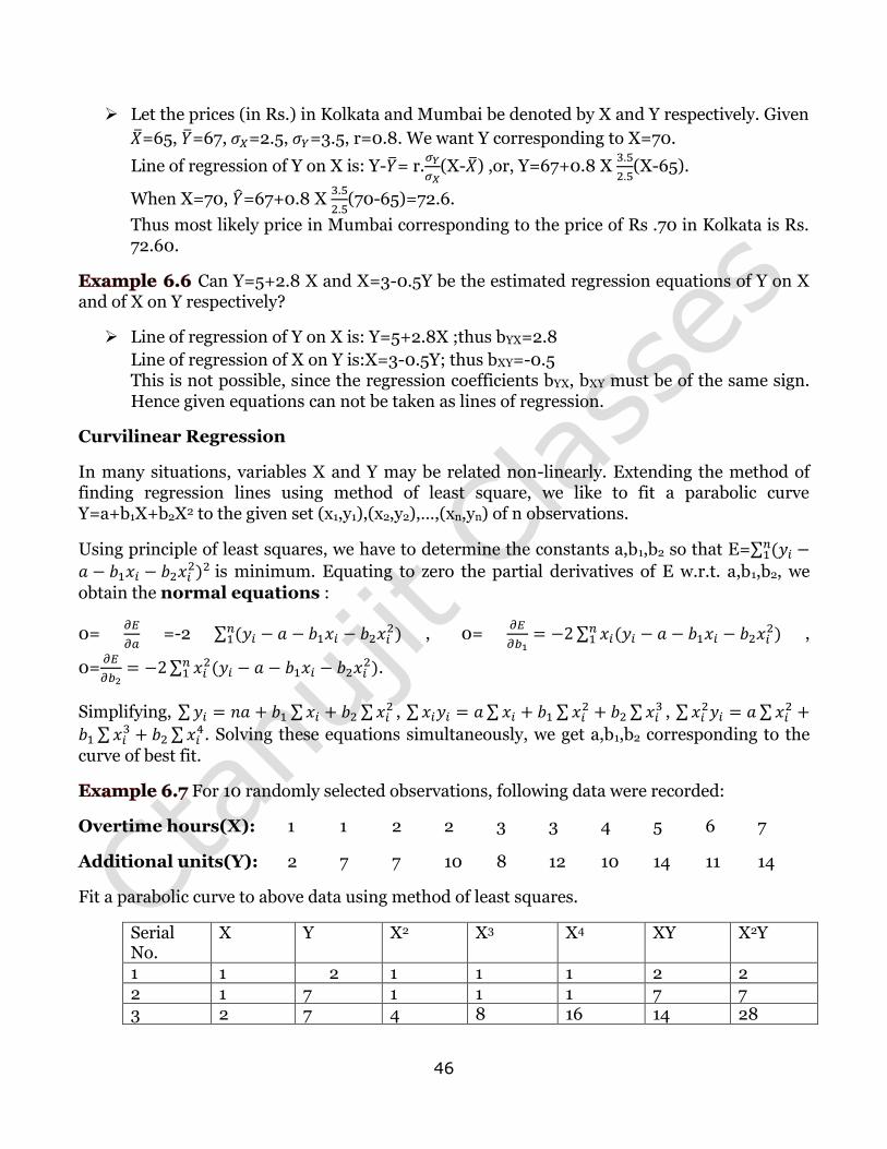
46
Let the prices (in Rs.) in Kolkata and Mumbai be denoted by X and Y respectively. Given
=65, =67, =2.5, =3.5, r=0.8. We want Y corresponding to X=70.
Line of regression of Y on X is: Y- = r.
(X- ) ,or, Y=67+0.8 X
(X-65).
When X=70, =67+0.8 X
(70-65)=72.6.
Thus most likely price in Mumbai corresponding to the price of Rs .70 in Kolkata is Rs. 72.60.
Can Y=5+2.8 X and X=3-0.5Y be the estimated regression equations of Y on X and of X on Y respectively?
Line of regression of Y on X is: Y=5+2.8X ;thus bYX=2.8
Line of regression of X on Y is:X=3-0.5Y; thus bXY=-0.5 This is not possible, since the regression coefficients bYX, bXY must be of the same sign. Hence given equations can not be taken as lines of regression.
Curvilinear Regression
In many situations, variables X and Y may be related non-linearly. Extending the method of finding regression lines using method of least square, we like to fit a parabolic curve Y=a+b1X+b2X2 to the given set (x1,y1),(x2,y2),…,(xn,yn) of n observations.
Using principle of least squares, we have to determine the constants a,b1,b2 so that E=∑
is minimum. Equating to zero the partial derivatives of E w.r.t. a,b1,b2, we
obtain the normal equations :
0=
=-2 ∑
, 0=
∑
,
0=
∑
.
Simplifying, ∑ ∑ ∑ , ∑ ∑ ∑
∑ , ∑
∑
∑ ∑
. Solving these equations simultaneously, we get a,b1,b2 corresponding to the
curve of best fit.
For 10 randomly selected observations, following data were recorded:
Overtime hours(X): 1 1 2 2 3 3 4 5 6 7
Additional units(Y): 2 7 7 10 8 12 10 14 11 14
Fit a parabolic curve to above data using method of least squares.
Serial No.
X Y X2 X3 X4 XY X2Y
1 1 2 1 1 1 2 2 2 1 7 1 1 1 7 7 3 2 7 4 8 16 14 28
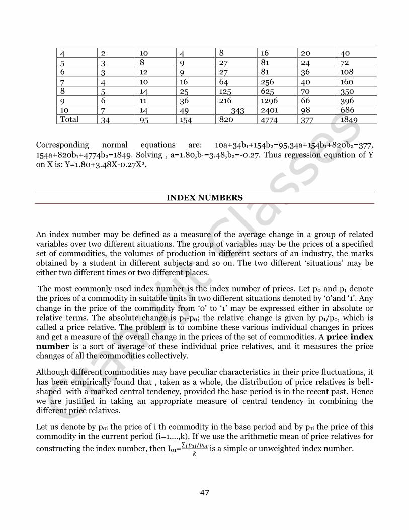
47
4 2 10 4 8 16 20 40 5 3 8 9 27 81 24 72 6 3 12 9 27 81 36 108 7 4 10 16 64 256 40 160 8 5 14 25 125 625 70 350 9 6 11 36 216 1296 66 396 10 7 14 49 343 2401 98 686 Total 34 95 154 820 4774 377 1849
Corresponding normal equations are: 10a+34b1+154b2=95,34a+154b1+820b2=377, 154a+820b1+4774b2=1849. Solving , a=1.80,b1=3.48,b2=-0.27. Thus regression equation of Y on X is: Y=1.80+3.48X-0.27X2.
INDEX NUMBERS
An index number may be defined as a measure of the average change in a group of related variables over two different situations. The group of variables may be the prices of a specified set of commodities, the volumes of production in different sectors of an industry, the marks obtained by a student in different subjects and so on. The two different ‘situations’ may be either two different times or two different places.
The most commonly used index number is the index number of prices. Let p0 and p1 denote the prices of a commodity in suitable units in two different situations denoted by ‘0’and ‘1’. Any change in the price of the commodity from ‘0’ to ‘1’ may be expressed either in absolute or relative terms. The absolute change is p1-p0; the relative change is given by p1/p0, which is called a price relative. The problem is to combine these various individual changes in prices and get a measure of the overall change in the prices of the set of commodities. A price index number is a sort of average of these individual price relatives, and it measures the price changes of all the commodities collectively.
Although different commodities may have peculiar characteristics in their price fluctuations, it has been empirically found that , taken as a whole, the distribution of price relatives is bell-shaped with a marked central tendency, provided the base period is in the recent past. Hence we are justified in taking an appropriate measure of central tendency in combining the different price relatives.
Let us denote by p0i the price of i th commodity in the base period and by p1i the price of this commodity in the current period (i=1,…,k). If we use the arithmetic mean of price relatives for
constructing the index number, then I01=∑
is a simple or unweighted index number.
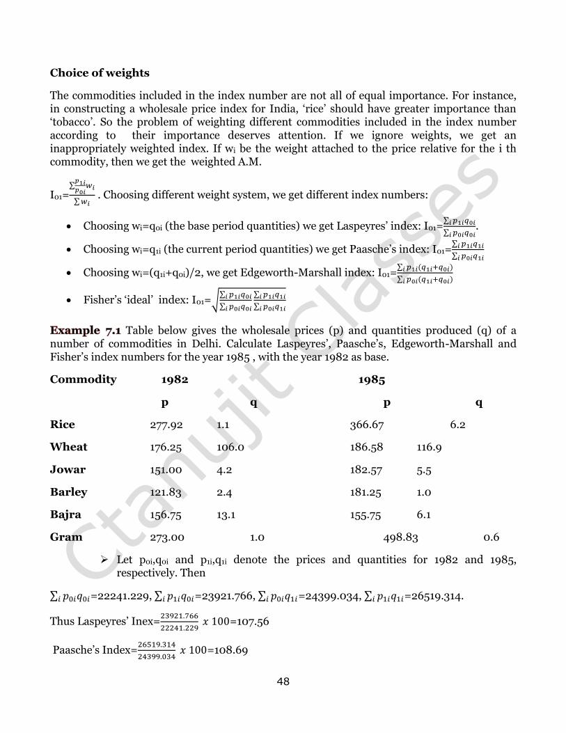
48
Choice of weights
The commodities included in the index number are not all of equal importance. For instance, in constructing a wholesale price index for India, ‘rice’ should have greater importance than ‘tobacco’. So the problem of weighting different commodities included in the index number according to their importance deserves attention. If we ignore weights, we get an inappropriately weighted index. If wi be the weight attached to the price relative for the i th commodity, then we get the weighted A.M.
I01=∑
∑ . Choosing different weight system, we get different index numbers:
Choosing wi=q0i (the base period quantities) we get Laspeyres’ index: I01=∑
∑ .
Choosing wi=q1i (the current period quantities) we get Paasche’s index: I01=∑
∑
Choosing wi=(q1i+q0i)/2, we get Edgeworth-Marshall index: I01=∑
∑
Fisher’s ‘ideal’ index: I01=√∑
∑
∑
∑
Table below gives the wholesale prices (p) and quantities produced (q) of a number of commodities in Delhi. Calculate Laspeyres’, Paasche’s, Edgeworth-Marshall and Fisher’s index numbers for the year 1985 , with the year 1982 as base.
Commodity 1982 1985
p q p q
Rice 277.92 1.1 366.67 6.2
Wheat 176.25 106.0 186.58 116.9
Jowar 151.00 4.2 182.57 5.5
Barley 121.83 2.4 181.25 1.0
Bajra 156.75 13.1 155.75 6.1
Gram 273.00 1.0 498.83 0.6
Let p0i,q0i and p1i,q1i denote the prices and quantities for 1982 and 1985, respectively. Then
∑ =22241.229, ∑ =23921.766, ∑ =24399.034, ∑ =26519.314.
Thus Laspeyres’ Inex=
=107.56
Paasche’s Index=
=108.69
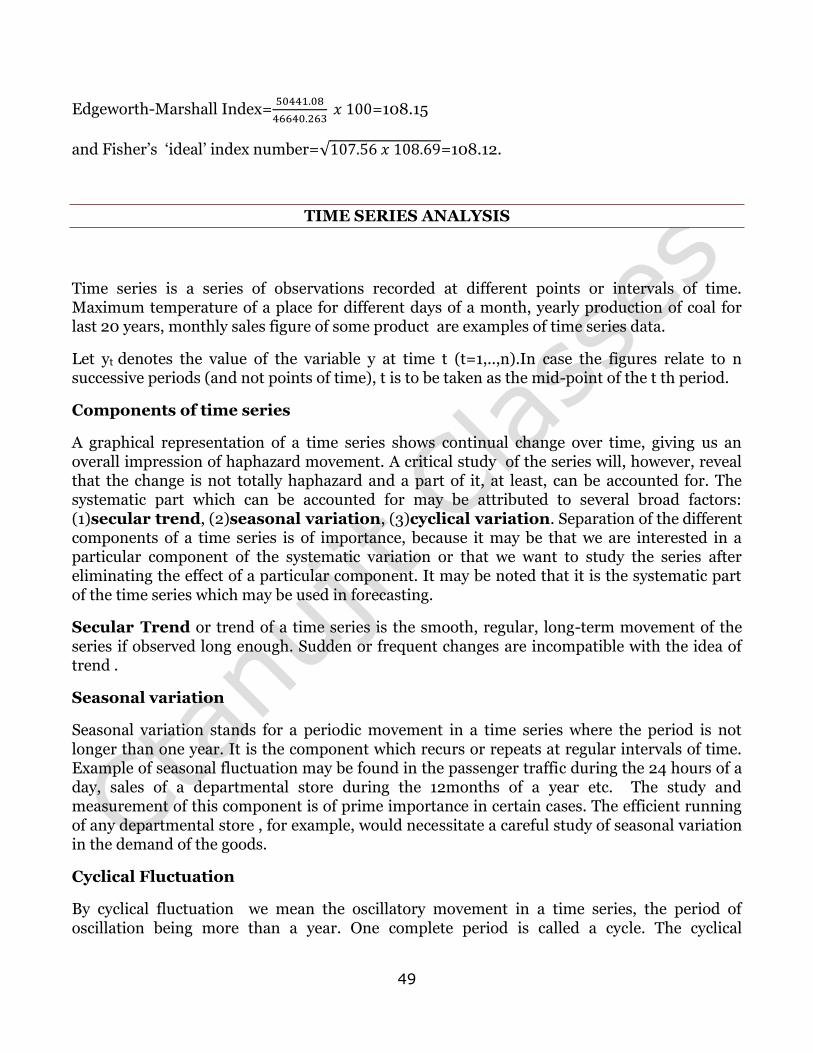
49
Edgeworth-Marshall Index=
=108.15
and Fisher’s ‘ideal’ index number=√ =108.12.
TIME SERIES ANALYSIS
Time series is a series of observations recorded at different points or intervals of time. Maximum temperature of a place for different days of a month, yearly production of coal for last 20 years, monthly sales figure of some product are examples of time series data.
Let yt denotes the value of the variable y at time t (t=1,..,n).In case the figures relate to n successive periods (and not points of time), t is to be taken as the mid-point of the t th period.
Components of time series
A graphical representation of a time series shows continual change over time, giving us an overall impression of haphazard movement. A critical study of the series will, however, reveal that the change is not totally haphazard and a part of it, at least, can be accounted for. The systematic part which can be accounted for may be attributed to several broad factors: (1)secular trend, (2)seasonal variation, (3)cyclical variation. Separation of the different components of a time series is of importance, because it may be that we are interested in a particular component of the systematic variation or that we want to study the series after eliminating the effect of a particular component. It may be noted that it is the systematic part of the time series which may be used in forecasting.
Secular Trend or trend of a time series is the smooth, regular, long-term movement of the series if observed long enough. Sudden or frequent changes are incompatible with the idea of trend .
Seasonal variation
Seasonal variation stands for a periodic movement in a time series where the period is not longer than one year. It is the component which recurs or repeats at regular intervals of time. Example of seasonal fluctuation may be found in the passenger traffic during the 24 hours of a day, sales of a departmental store during the 12months of a year etc. The study and measurement of this component is of prime importance in certain cases. The efficient running of any departmental store , for example, would necessitate a careful study of seasonal variation in the demand of the goods.
Cyclical Fluctuation
By cyclical fluctuation we mean the oscillatory movement in a time series, the period of oscillation being more than a year. One complete period is called a cycle. The cyclical
50
fluctuations are not necessarily periodic, since the length of the cycle as also the intensity of fluctuations may change from one cycle to another.
Irregular Fluctuation
This component is either wholly unaccountable or are caused by such unforeseen events as wars, floods, strikes etc.
Estimation of secular trend in a time series by elimination of seasonal and cyclical fluctuation
In order to measure the trend , we are to eliminate from the time series the other three components. If the period of seasonal fluctuations be a year, then the yearly totals or tearly averages will be free from the seasonal effect. Thus, in determining the trend from monthly data, it is customary to start with the yearly totals or averages, which are free from seasonal effects. The monthly trend values can be obtained from the annual trend values by interpolation.to eliminate the other two components, viz. the cyclical and the irregular, we may consider the following methods:
Method of moving averages
The simple moving average of period k of a time series gives a new series of arithmetic means, each of k successive observations of the time series. We start with the first k observations. At the next stage, we leave the first and include the (k+1)th observation. This process is repeated until we arrive at the last k observations. Each of these means is centered against the time which is the mid-point of the time interval included in the calculation of the moving average. Thus when k, the period of moving average, is odd, the moving average values correspond to tabulated time values for which the time series is given. When k is even,the moving average falls midway between two tabulated values. In this case, we calculate a subsequent two-item moving average to make the resulting moving average values correspond to the tabulated time periods.
The interpolation ofsimple moving averages is very simple. A k-point moving average may be interpreted as the estimated value for the middle of the period covered from successive linear curves fitted through the first k points, through the 2nd to the (k+1)th values and so on, and lastly through the last k points.
Consider the first k points y1,…,yk. Let the origin be shifted to the middle of the period so that ∑ =0. The normal equations for fitting a curve Y=a+bt through y1,…,yk are
∑ =ka+b∑ ,∑ ∑ ∑
So that ∑
∑
∑ . Hence the estimated value for the middle of the period covered
,that is, for t=0, from the curve Y= + t is , which is the first moving average value. Similarly it can be shown that the estimated value from the fitted linear curve through y2,…,yk+1 would be
∑
, the second moving average value and so on.
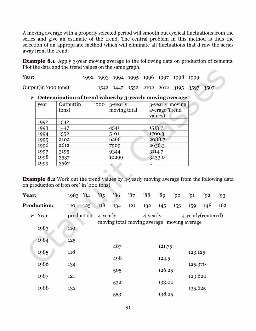
51
A moving average with a properly selected period will smooth out cyclical fluctuations from the series and give an estimate of the trend. The central problem in this method is thus the selection of an appropriate method which will eliminate all fluctuations that d raw the series away from the trend.
Apply 3-year moving average to the following data on production of cements. Plot the data and the trend values on the same graph.
Year: 1992 1993 1994 1995 1996 1997 1998 1999
Output(in ‘000 tons) 1542 1447 1552 2102 2612 3195 3597 3567
Determination of trend values by 3-yearly moving average
year Output(in ‘000 tons)
3-yearly moving total
3-yearly moving average(Trend values)
1992 1542 .. .. 1993 1447 4541 1513.7 1994 1552 5101 1700.3 1995 2102 6266 2088.7 1996 2612 7909 2636.3 1997 3195 9344 3114.7 1998 3537 10299 3433.0 1999 3567 .. ..
Work out the trend values by 4-yearly moving average from the following data on production of iron ore( in ‘000 tons)
Year: 1983 ’84 ’85 ’86 ’87 ’88 ’89 ’90 ’91 ’92 ‘93
Production: 110 125 118 134 121 132 145 155 159 148 162
Year production 4-yearly 4-yearly 4-yearly(centered)
moving total moving average moving average 1983 110 1984 125 487 121.75 1985 118 123.125 498 124.5 1986 134 125.370 505 126.25 1987 121 129.620 532 133.00 1988 132 135.625 553 138.25
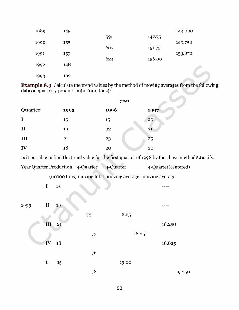
52
1989 145 143.000 591 147.75 1990 155 149.750 607 151.75 1991 159 153.870 624 156.00 1992 148 1993 162
Calculate the trend values by the method of moving averages from the following data on quarterly production(in ‘000 tons):
year
Quarter 1995 1996 1997
I 15 15 20
II 19 22 21
III 21 23 25
IV 18 20 20
Is it possible to find the trend value for the first quarter of 1998 by the above method? Justify.
Year Quarter Production 4-Quarter 4-Quarter 4-Quarter(centered)
(in’000 tons) moving total moving average moving average
I 15 ----
1995 II 19 ----
73 18.25
III 21 18.250
73 18.25
IV 18 18.625
76
I 15 19.00
78 19.250
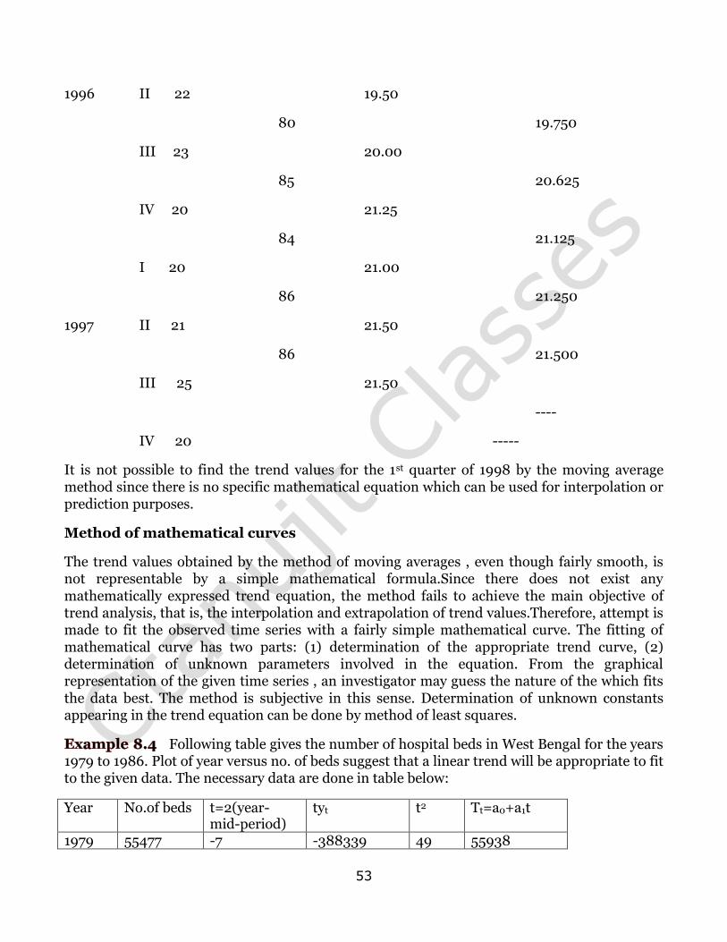
53
1996 II 22 19.50
80 19.750
III 23 20.00
85 20.625
IV 20 21.25
84 21.125
I 20 21.00
86 21.250
1997 II 21 21.50
86 21.500
III 25 21.50
----
IV 20 -----
It is not possible to find the trend values for the 1st quarter of 1998 by the moving average method since there is no specific mathematical equation which can be used for interpolation or prediction purposes.
Method of mathematical curves
The trend values obtained by the method of moving averages , even though fairly smooth, is not representable by a simple mathematical formula.Since there does not exist any mathematically expressed trend equation, the method fails to achieve the main objective of trend analysis, that is, the interpolation and extrapolation of trend values.Therefore, attempt is made to fit the observed time series with a fairly simple mathematical curve. The fitting of mathematical curve has two parts: (1) determination of the appropriate trend curve, (2) determination of unknown parameters involved in the equation. From the graphical representation of the given time series , an investigator may guess the nature of the which fits the data best. The method is subjective in this sense. Determination of unknown constants appearing in the trend equation can be done by method of least squares.
Following table gives the number of hospital beds in West Bengal for the years 1979 to 1986. Plot of year versus no. of beds suggest that a linear trend will be appropriate to fit to the given data. The necessary data are done in table below:
Year No.of beds t=2(year- mid-period)
tyt t2 Tt=a0+a1t
1979 55477 -7 -388339 49 55938
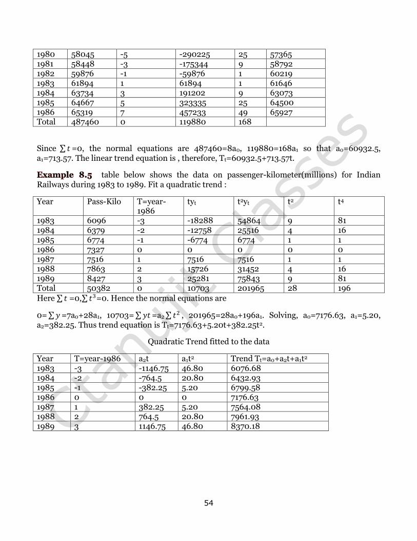
54
1980 58045 -5 -290225 25 57365 1981 58448 -3 -175344 9 58792 1982 59876 -1 -59876 1 60219 1983 61894 1 61894 1 61646 1984 63734 3 191202 9 63073 1985 64667 5 323335 25 64500 1986 65319 7 457233 49 65927 Total 487460 0 119880 168
Since ∑ =0, the normal equations are 487460=8a0, 119880=168a1 so that a0=60932.5, a1=713.57. The linear trend equation is , therefore, Tt=60932.5+713.57t.
table below shows the data on passenger-kilometer(millions) for Indian Railways during 1983 to 1989. Fit a quadratic trend :
Year Pass-Kilo T=year-1986
tyt t2yt t2 t4
1983 6096 -3 -18288 54864 9 81 1984 6379 -2 -12758 25516 4 16 1985 6774 -1 -6774 6774 1 1 1986 7327 0 0 0 0 0 1987 7516 1 7516 7516 1 1 1988 7863 2 15726 31452 4 16 1989 8427 3 25281 75843 9 81 Total 50382 0 10703 201965 28 196
Here ∑ =0,∑ =0. Hence the normal equations are
0= ∑ =7a0+28a1, 10703= ∑ =a2 ∑ , 201965=28a0+196a1. Solving, a0=7176.63, a1=5.20, a2=382.25. Thus trend equation is Tt=7176.63+5.20t+382.25t2.
Quadratic Trend fitted to the data
Year T=year-1986 a2t a1t2 Trend Tt=a0+a2t+a1t2 1983 -3 -1146.75 46.80 6076.68 1984 -2 -764.5 20.80 6432.93 1985 -1 -382.25 5.20 6799.58 1986 0 0 0 7176.63 1987 1 382.25 5.20 7564.08 1988 2 764.5 20.80 7961.93 1989 3 1146.75 46.80 8370.18
LINEAR PROGRAMMING
CHAPTER I
Mathematical formulation of Linear Programming Problem
Let us consider two real life situations to understand what we mean by a
programming problem. For any industry, the objective is to earn maximum profit
by selling products which are produced with limited available resources, keeping
the cost of production at a minimum. For a housewife the aim is to buy provisions
for the family at a minimum cost which will satisfy the needs of the family.
All these type of problems can be done mathematically by formulating a problem
which is known as a programming problem. Some restrictions or constraints are to
be adopted to formulate the problem. The function which is to be maximized or
minimized is called the objective function. If in a programming problem the
constraints and the objective function are of linear type then the problem is called a
linear programming problem. There are various types of linear programming
problems which we will consider through some examples.
Examples
1. (Production allocation problem) Four different type of metals, namely, iron,
copper, zinc and manganese are required to produce commodities A, B and
C. To produce one unit of A, 40kg iron, 30kg copper, 7kg zinc and 4kg
manganese are needed. Similarly, to produce one unit of B, 70kg iron, 14kg
copper and 9kg manganese are needed and for producing one unit of C, 50kg
iron, 18kg copper and 8kg zinc are required. The total available quantities of
metals are 1 metric ton iron, 5 quintals copper, 2 quintals of zinc and
manganese each. The profits are Rs 300, Rs 200 and Rs 100 by selling one
unit of A, B and C respectively. Formulate the problem mathematically.
Solution: Let z be the total profit and the problem is to maximize z(called
the objective function). We write below the given data in a tabular form:
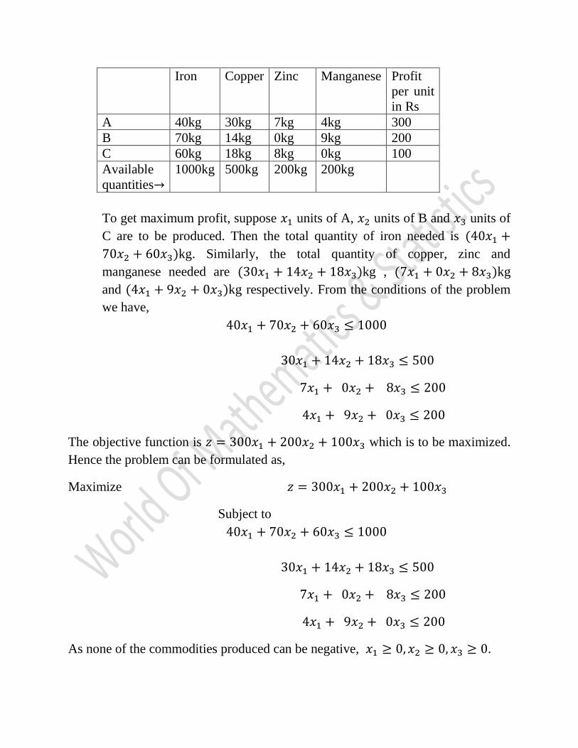
Iron Copper Zinc Manganese Profit
per unit
in Rs
A 40kg 30kg 7kg 4kg 300
B 70kg 14kg 0kg 9kg 200
C 60kg 18kg 8kg 0kg 100
Available
quantities
1000kg 500kg 200kg 200kg
To get maximum profit, suppose units of A, units of B and units of
C are to be produced. Then the total quantity of iron needed is
kg. Similarly, the total quantity of copper, zinc and
manganese needed are kg , kg
and kg respectively. From the conditions of the problem
we have,
The objective function is which is to be maximized.
Hence the problem can be formulated as,
Maximize
Subject to
As none of the commodities produced can be negative, .
All these inequalities are known as constraints or restrictions.
2. (Diet problem) A patient needs daily 5mg, 20mg and 15mg of vitamins A, B
and C respectively. The vitamins available from a mango are 0.5mg of A,
1mg of B, 1mg of C, that from an orange is 2mg of B, 3mg of C and that
from an apple is 0.5mg of A, 3mg of B, 1mg of C. If the cost of a mango, an
orange and an apple be Rs 0.50, Rs 0.25 and Rs 0.40 respectively, find the
minimum cost of buying the fruits so that the daily requirement of the
patient be met. Formulate the problem mathematically.
Solution: The problem is to find the minimum cost of buying the fruits. Let z be
the objective function. Let the number of mangoes, oranges and apples to be
bought so that the cost is minimum and to get the minimum daily requirement
of the vitamins be respectively. Then the objective function is given
by
From the conditions of the problem
and
Hence the problem is
Minimize .
Subject to
and
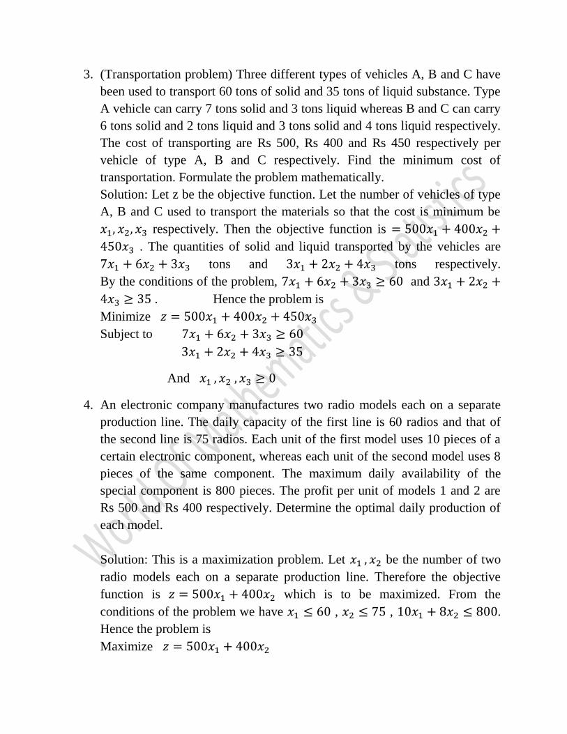
3. (Transportation problem) Three different types of vehicles A, B and C have
been used to transport 60 tons of solid and 35 tons of liquid substance. Type
A vehicle can carry 7 tons solid and 3 tons liquid whereas B and C can carry
6 tons solid and 2 tons liquid and 3 tons solid and 4 tons liquid respectively.
The cost of transporting are Rs 500, Rs 400 and Rs 450 respectively per
vehicle of type A, B and C respectively. Find the minimum cost of
transportation. Formulate the problem mathematically.
Solution: Let z be the objective function. Let the number of vehicles of type
A, B and C used to transport the materials so that the cost is minimum be
respectively. Then the objective function is
. The quantities of solid and liquid transported by the vehicles are
tons and tons respectively.
By the conditions of the problem, and
. Hence the problem is
Minimize
Subject to
And
4. An electronic company manufactures two radio models each on a separate
production line. The daily capacity of the first line is 60 radios and that of
the second line is 75 radios. Each unit of the first model uses 10 pieces of a
certain electronic component, whereas each unit of the second model uses 8
pieces of the same component. The maximum daily availability of the
special component is 800 pieces. The profit per unit of models 1 and 2 are
Rs 500 and Rs 400 respectively. Determine the optimal daily production of
each model.
Solution: This is a maximization problem. Let be the number of two
radio models each on a separate production line. Therefore the objective
function is which is to be maximized. From the
conditions of the problem we have , , .
Hence the problem is
Maximize
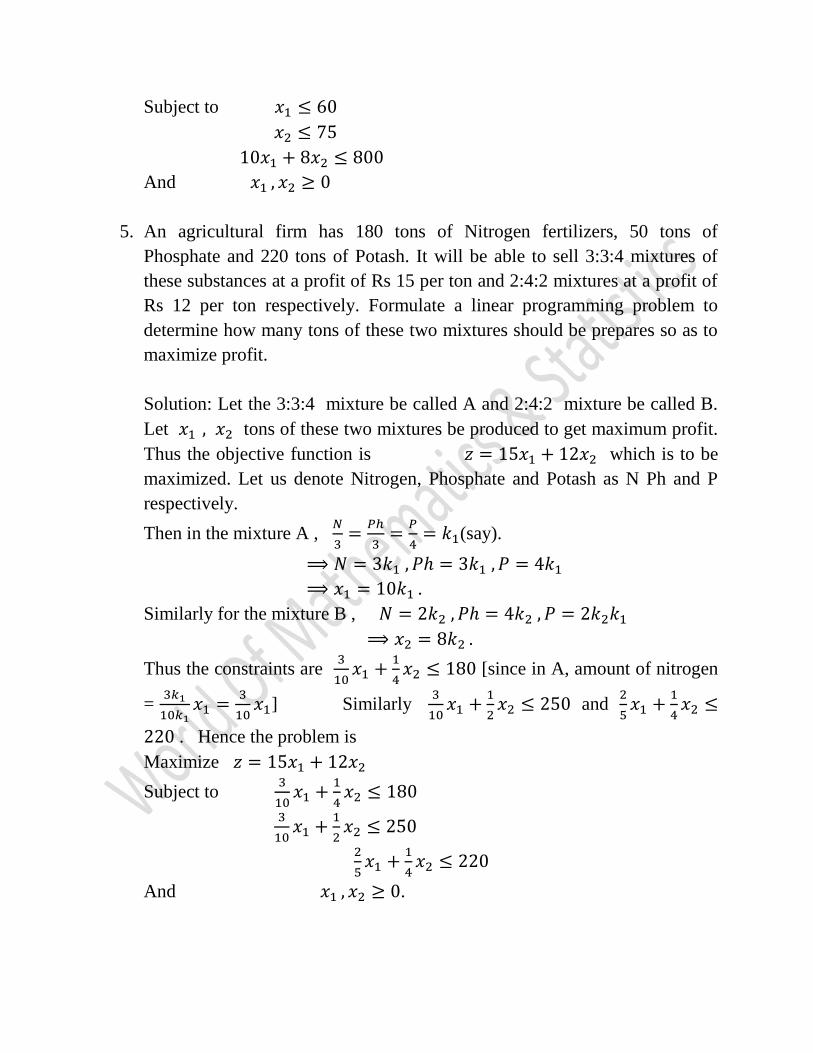
Subject to
And
5. An agricultural firm has 180 tons of Nitrogen fertilizers, 50 tons of
Phosphate and 220 tons of Potash. It will be able to sell 3:3:4 mixtures of
these substances at a profit of Rs 15 per ton and 2:4:2 mixtures at a profit of
Rs 12 per ton respectively. Formulate a linear programming problem to
determine how many tons of these two mixtures should be prepares so as to
maximize profit.
Solution: Let the 3:3:4 mixture be called A and 2:4:2 mixture be called B.
Let tons of these two mixtures be produced to get maximum profit.
Thus the objective function is which is to be
maximized. Let us denote Nitrogen, Phosphate and Potash as N Ph and P
respectively.
Then in the mixture A ,
(say).
.
Similarly for the mixture B ,
.
Thus the constraints are
[since in A, amount of nitrogen
=
] Similarly
and
. Hence the problem is
Maximize
Subject to
And .
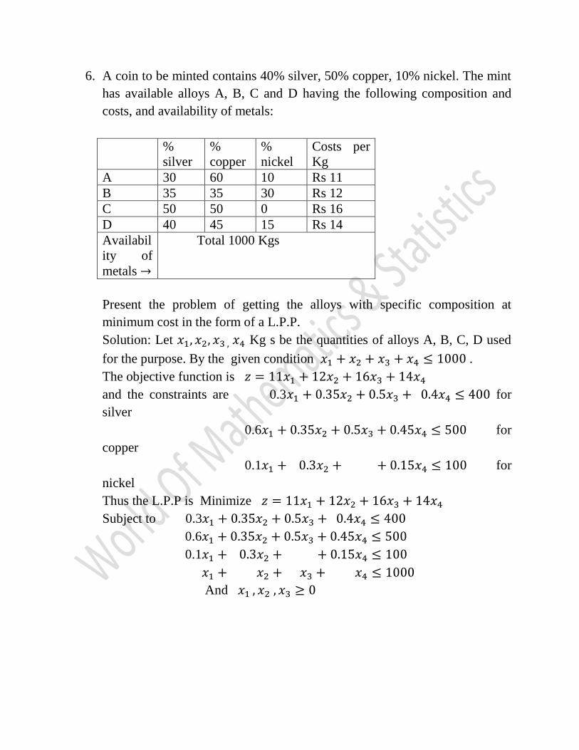
6. A coin to be minted contains 40% silver, 50% copper, 10% nickel. The mint
has available alloys A, B, C and D having the following composition and
costs, and availability of metals:
%
silver
%
copper
%
nickel
Costs per
Kg
A 30 60 10 Rs 11
B 35 35 30 Rs 12
C 50 50 0 Rs 16
D 40 45 15 Rs 14
Availabil
ity of
metals
Total 1000 Kgs
Present the problem of getting the alloys with specific composition at
minimum cost in the form of a L.P.P.
Solution: Let Kg s be the quantities of alloys A, B, C, D used
for the purpose. By the given condition .
The objective function is
and the constraints are 0.3 for
silver
0.6 for
copper
0.1 for
nickel
Thus the L.P.P is Minimize
Subject to 0.3
0.6
0.1
And
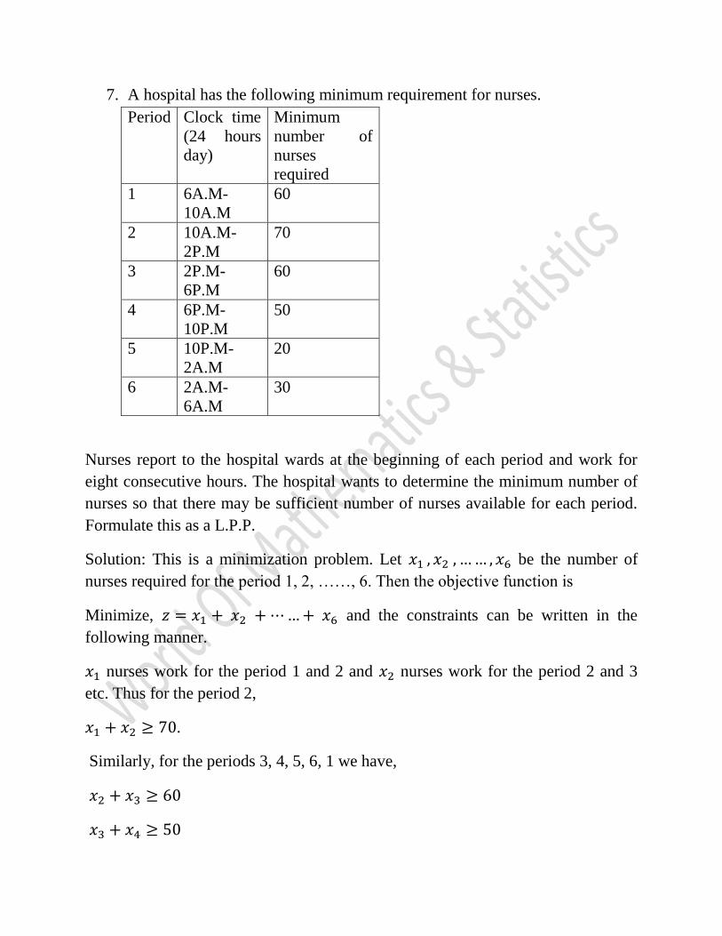
7. A hospital has the following minimum requirement for nurses.
Period Clock time
(24 hours
day)
Minimum
number of
nurses
required
1 6A.M-
10A.M
60
2 10A.M-
2P.M
70
3 2P.M-
6P.M
60
4 6P.M-
10P.M
50
5 10P.M-
2A.M
20
6 2A.M-
6A.M
30
Nurses report to the hospital wards at the beginning of each period and work for
eight consecutive hours. The hospital wants to determine the minimum number of
nurses so that there may be sufficient number of nurses available for each period.
Formulate this as a L.P.P.
Solution: This is a minimization problem. Let be the number of
nurses required for the period 1, 2, ……, 6. Then the objective function is
Minimize, and the constraints can be written in the
following manner.
nurses work for the period 1 and 2 and nurses work for the period 2 and 3
etc. Thus for the period 2,
.
Similarly, for the periods 3, 4, 5, 6, 1 we have,
,
Mathematical formulation of a L.P.P
From the discussion above, now we can mathematically formulate a general Linear
Programming Problem which can be stated as follows.
Find out a set of values which will optimize (either maximize or
minimize) the linear function
Subject to the restrictions
……………………………………………..
And the non-negative restrictions where
are all constants and are
variables. Each of the linear expressions on the left hand side connected to the
corresponding constants on the right side by only one of the signs , = and ,is
known as a constraint. A constraint is either an equation or an inequation.
The linear function is known as the objective
function.
By using the matrix and vector notation the problem can be expressed in a compact
form as
Optimize subject to the restrictions ,
where [ ] is a m x n coefficient matrix.,
is a n-component column vector, which is known as a cost
or price vector,
is a n-component column vector, which is known as
decision variable vector or legitimate variable vector and
is a m-component column vector, which is known as
requirement vector.
In all practical discussions, . If some of them are negative, we make them
by multiplying both sides of the inequality by (-1).
If all the constraints are equalities, then the L.P.P is reduced to
Optimize subject to .
This form is called the standard form.
Feasible solution to a L.P.P: A set of values of the variables, which satisfy all the
constraints and all the non-negative restrictions of the variables, is known as the
feasible solution (F.S.) to the L.P.P.
Optimal solution to a L.P.P: A feasible solution to a L.P.P which makes the
objective function optimal is known as the optimal solution to the L.P.P
There are two ways of solving a linear programming problem: (1) Geometrical
method and (2) Algebraic method.
A particular L.P.P is either a minimization or a maximization problem. The
problem of minimization of the objective function is nothing but the problem of
maximization of the function and vice versa and with
the same set of constraints and the same solution set.
Graphical or Geometrical Method of Solving a Linear Programming Problem
We will illustrate the method by giving examples.
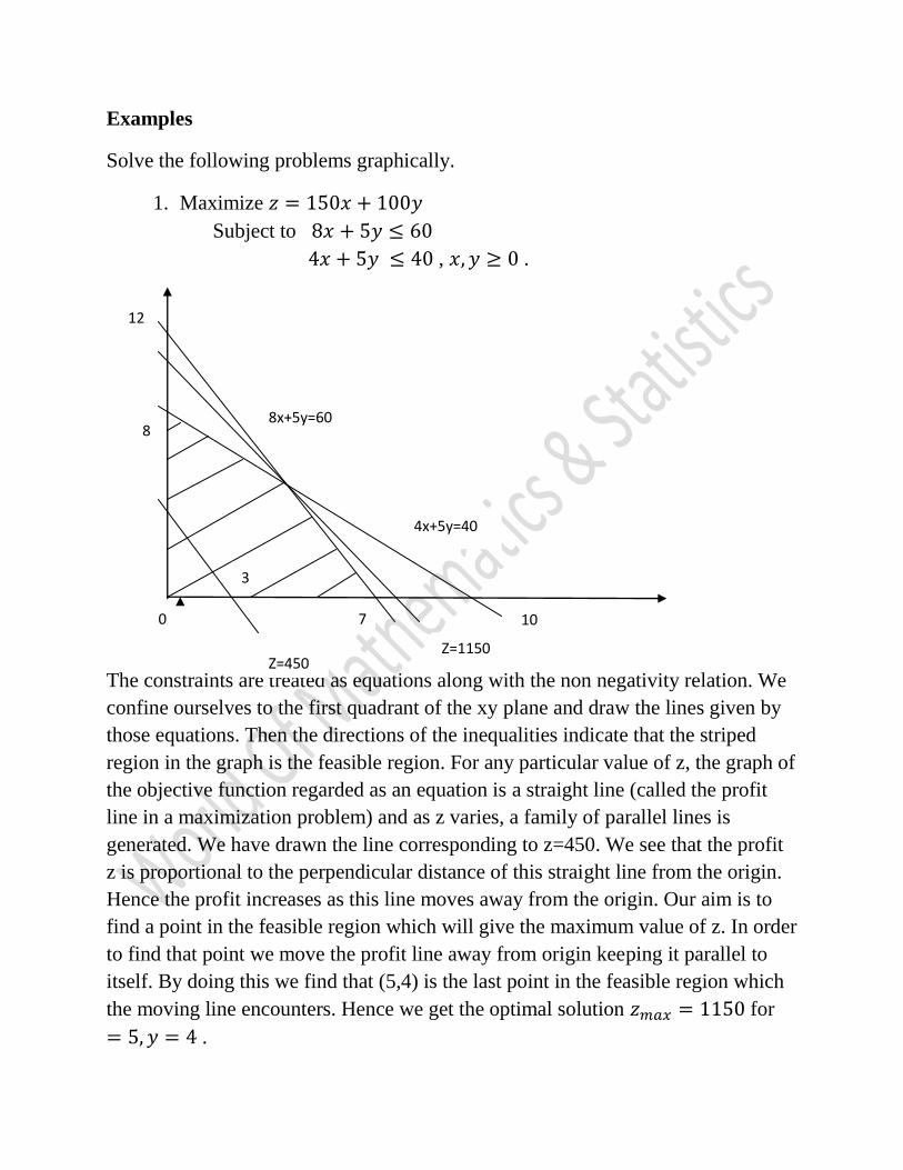
Examples
Solve the following problems graphically.
1. Maximize
Subject to
, .
The constraints are treated as equations along with the non negativity relation. We
confine ourselves to the first quadrant of the xy plane and draw the lines given by
those equations. Then the directions of the inequalities indicate that the striped
region in the graph is the feasible region. For any particular value of z, the graph of
the objective function regarded as an equation is a straight line (called the profit
line in a maximization problem) and as z varies, a family of parallel lines is
generated. We have drawn the line corresponding to z=450. We see that the profit
z is proportional to the perpendicular distance of this straight line from the origin.
Hence the profit increases as this line moves away from the origin. Our aim is to
find a point in the feasible region which will give the maximum value of z. In order
to find that point we move the profit line away from origin keeping it parallel to
itself. By doing this we find that (5,4) is the last point in the feasible region which
the moving line encounters. Hence we get the optimal solution for
.
12
8x+5y=60 8
4x+5y=40
3
10 7 0
Z=1150 Z=450
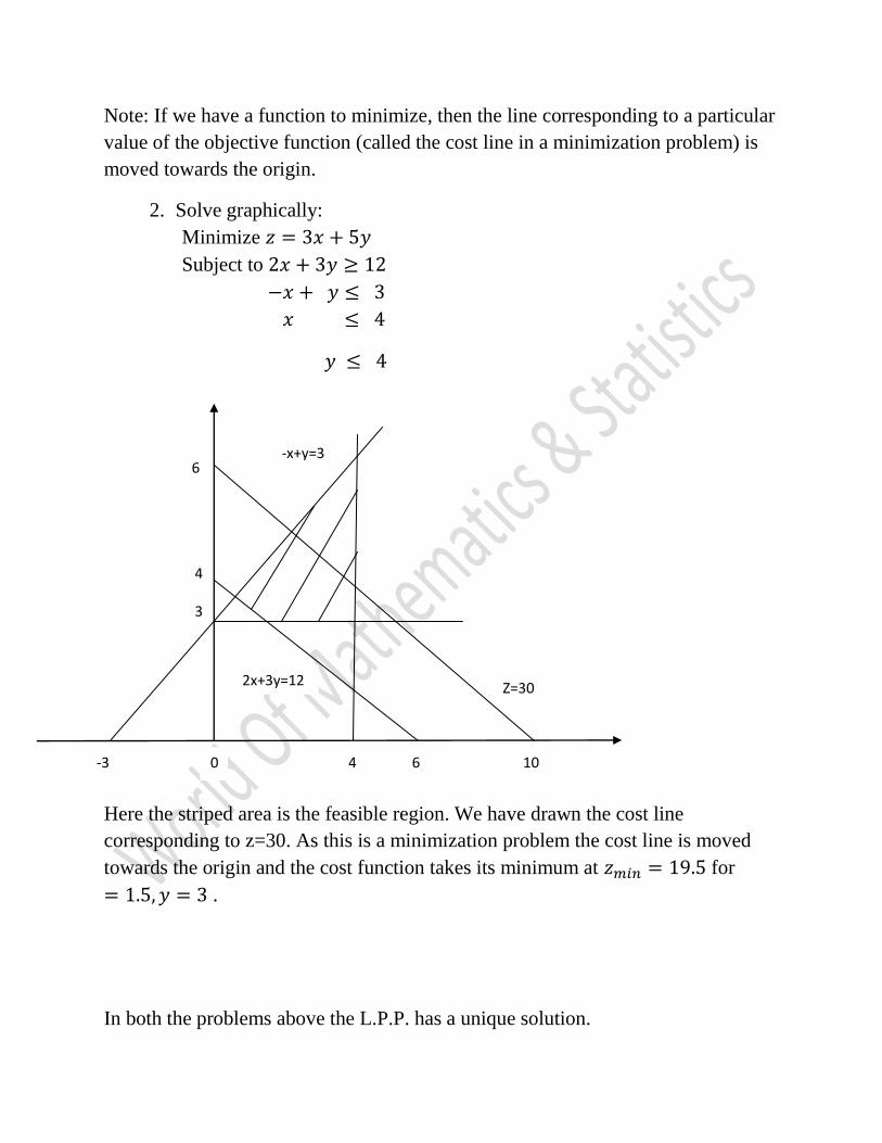
Note: If we have a function to minimize, then the line corresponding to a particular
value of the objective function (called the cost line in a minimization problem) is
moved towards the origin.
2. Solve graphically:
Minimize
Subject to
Here the striped area is the feasible region. We have drawn the cost line
corresponding to z=30. As this is a minimization problem the cost line is moved
towards the origin and the cost function takes its minimum at for
.
In both the problems above the L.P.P. has a unique solution.
-x+y=3
6
4
3
Z=30 2x+3y=12
10 6 4 0 -3
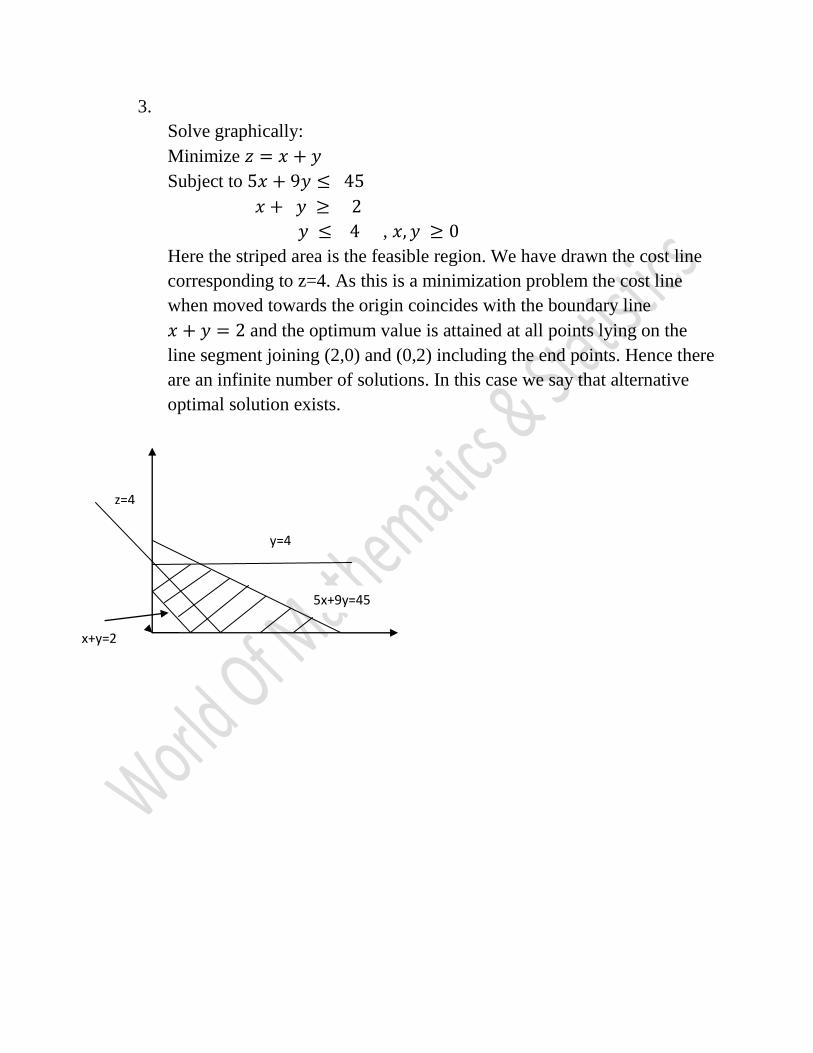
3.
Solve graphically:
Minimize
Subject to
,
Here the striped area is the feasible region. We have drawn the cost line
corresponding to z=4. As this is a minimization problem the cost line
when moved towards the origin coincides with the boundary line
and the optimum value is attained at all points lying on the
line segment joining (2,0) and (0,2) including the end points. Hence there
are an infinite number of solutions. In this case we say that alternative
optimal solution exists.
z=4
y=4
5x+9y=45
x+y=2
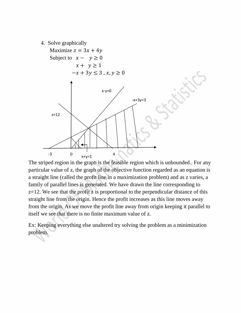
4. Solve graphically
Maximize
Subject to
,
The striped region in the graph is the feasible region which is unbounded.. For any
particular value of z, the graph of the objective function regarded as an equation is
a straight line (called the profit line in a maximization problem) and as z varies, a
family of parallel lines is generated. We have drawn the line corresponding to
z=12. We see that the profit z is proportional to the perpendicular distance of this
straight line from the origin. Hence the profit increases as this line moves away
from the origin. As we move the profit line away from origin keeping it parallel to
itself we see that there is no finite maximum value of z.
Ex: Keeping everything else unaltered try solving the problem as a minimization
problem.
x-y=0
-x+3y=3
z=12
x+y=1 4 -3 0
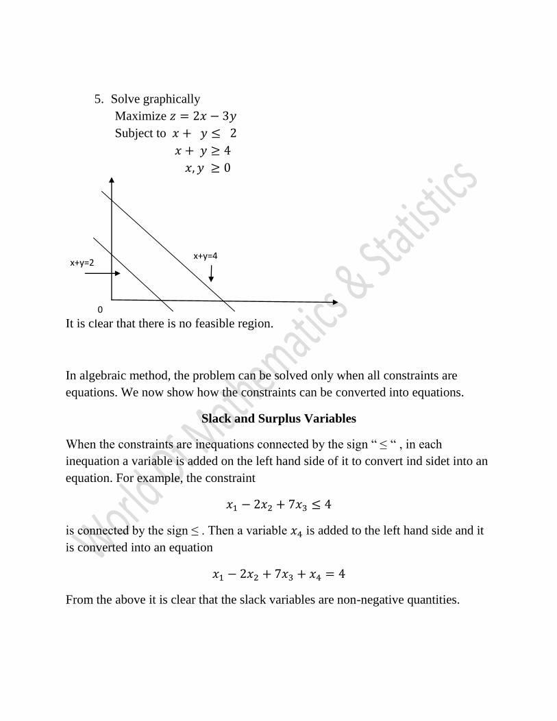
5. Solve graphically
Maximize
Subject to
It is clear that there is no feasible region.
In algebraic method, the problem can be solved only when all constraints are
equations. We now show how the constraints can be converted into equations.
Slack and Surplus Variables
When the constraints are inequations connected by the sign “ ≤ “ , in each
inequation a variable is added on the left hand side of it to convert ind sidet into an
equation. For example, the constraint
is connected by the sign ≤ . Then a variable is added to the left hand side and it
is converted into an equation
From the above it is clear that the slack variables are non-negative quantities.
x+y=2
x+y=4
0
If the constraints are connected by “ ≥ “ ,in each inequation a variable is subtracted
from the left hand side to convert it into an equation. These variables are known as
surplus variables. For example,
is converted into an equation by subtracting a variable from the left hand side.
The surplus variables are also non-negative quantities.
Let a general L.P.P containing r variables and m constraints be
Optimize
subject to
where one and only one of the signs holds for each constraint, but the signs
may vary from one constraint to another. Let constraints out of the be
inequations ( ). Then introducing k slack or surplus variables
, one to each of the inequations, all constraints can
be converted into equations containing n variables. We further assume that .
The objective function is similarly accommodated with k slack or surplus variables
, the cost components of these variables are assumed to be
zero. Then the adjusted objective function is
, and then the
problem can be written as
Optimize subject to ,
where is an matrix , known as coefficient matrix given by
,
where is a column vector associated with the vector
.
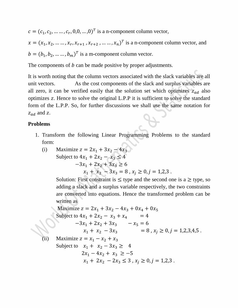
is a n-component column vector,
is a n-component column vector, and
is a m-component column vector.
The components of can be made positive by proper adjustments.
It is worth noting that the column vectors associated with the slack variables are all
unit vectors. As the cost components of the slack and surplus variables are
all zero, it can be verified easily that the solution set which optimizes also
optimizes . Hence to solve the original L.P.P it is sufficient to solve the standard
form of the L.P.P. So, for further discussions we shall use the same notation for
and .
Problems
1. Transform the following Linear Programming Problems to the standard
form:
(i) Maximize
Subject to
, .
Solution: First constraint is type and the second one is a type, so
adding a slack and a surplus variable respectively, the two constraints
are converted into equations. Hence the transformed problem can be
written as
Maximize
Subject to
, .
(ii) Maximize
Subject to
, .
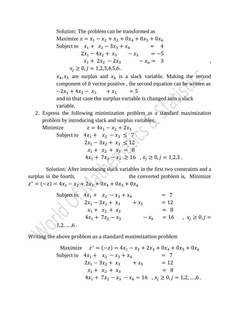
Solution: The problem can be transformed as
Maximize
Subject to
,
.
are surplus and is a slack variable. Making the second
component of vector positive , the second equation can be written as
slack
variable.
2. Express the following minimization problem as a standard maximization
problem by introducing slack and surplus variables.
Minimize
Subject to
, .
Solution: After introducing slack variables in the first two constraints and a
surplus in the fourth, the converted problem is, Minimize
Subject to
,
.
m
Maximize
Subject to
, .
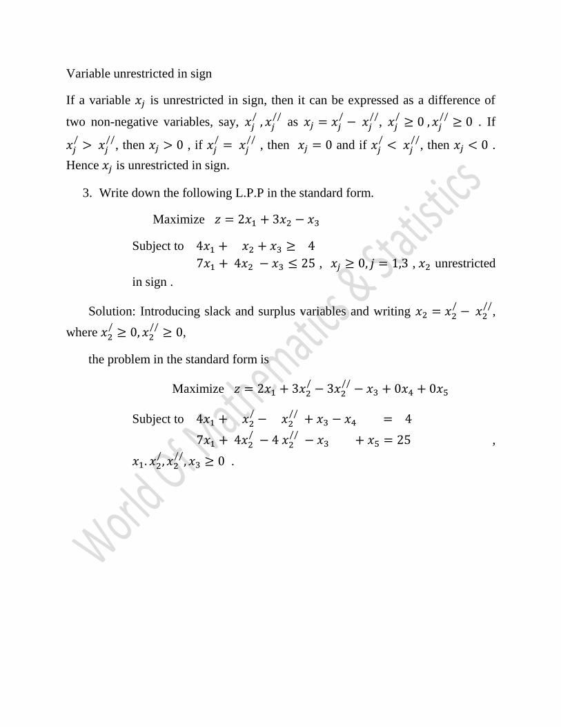
Variable unrestricted in sign
If a variable is unrestricted in sign, then it can be expressed as a difference of
two non-negative variables, say,
as
,
. If
, then , if
, then and if
, then .
Hence is unrestricted in sign.
3. Write down the following L.P.P in the standard form.
Maximize
Subject to
, , unrestricted
in sign .
Solution: Introducing slack and surplus variables and writing
,
where
,
the problem in the standard form is
Maximize
Subject to
,
.

TOP 10 PLACES FOR M.A./M.SC
ECONOMICS IN INDIA:
1. Indian Statistical Institute
2. Delhi School of Economics
3. Indira Gandhi Institute of
Development Research
4. Jawaharlal Nehru University
5. Centre for Development Studies
6. Madras School of Economics
7. South Asian University, Delhi
8. Gokhale Institute of Politics and
Economics
9. University of Hyderabad
10. Jamia Millia Islamia
Recommended