Lecture Notes
Wave Equations of Relativistic Quantum
Mechanics
Dr. Matthias LienertEberhard-Karls Universität Tübingen
Winter Semester 2018/19

2
Contents
1 Background 51.1 Basics of non-relativistic quantum mechanics . . . . . . . . . . . . . . 61.2 Basics of special relativity . . . . . . . . . . . . . . . . . . . . . . . . 9
2 The Poincaré group 132.1 Lorentz transformations. . . . . . . . . . . . . . . . . . . . . . . . . . 132.2 Poincaré transformations . . . . . . . . . . . . . . . . . . . . . . . . . 142.3 Invariance of wave equations . . . . . . . . . . . . . . . . . . . . . . . 172.4 Wish list for a relativistic wave equation . . . . . . . . . . . . . . . . 18
3 The Klein-Gordon equation 193.1 Derivation . . . . . . . . . . . . . . . . . . . . . . . . . . . . . . . . . 193.2 Physical properties . . . . . . . . . . . . . . . . . . . . . . . . . . . . 203.3 Solution theory . . . . . . . . . . . . . . . . . . . . . . . . . . . . . . 23
4 The Dirac equation 334.1 Derivation . . . . . . . . . . . . . . . . . . . . . . . . . . . . . . . . . 334.2 Relativistic invariance of the Dirac equation . . . . . . . . . . . . . . 374.3 Discrete Transformations. . . . . . . . . . . . . . . . . . . . . . . . . 444.4 Physical properties . . . . . . . . . . . . . . . . . . . . . . . . . . . . 454.5 Solution theory . . . . . . . . . . . . . . . . . . . . . . . . . . . . . . 50
4.5.1 Classical solutions . . . . . . . . . . . . . . . . . . . . . . . . . 504.5.2 Hilbert space valued solutions . . . . . . . . . . . . . . . . . . 51
5 The multi-time formalism 575.1 Motivation . . . . . . . . . . . . . . . . . . . . . . . . . . . . . . . . . 575.2 Evolution equations . . . . . . . . . . . . . . . . . . . . . . . . . . . . 595.3 Probability conservation and generalized Born rule . . . . . . . . . . 635.4 An interacting multi-time model in 1+1 dimensions . . . . . . . . . . 67
3

4 CONTENTS

1. Background
In this course, we will discuss relativistic quantum mechanical wave equations suchas the Klein-Gordon equation(
1
c2
∂
∂t2−∆ +
m2c2
~2
)ψ(t,x) = 0 (1.1)
and the Dirac equation3∑
µ=0
i~γµ∂ψ
∂xµ−mcψ = 0, (1.2)
where γµ, µ = 0, 1, 2, 3 are certain 4× 4 matrices.The basic motivation is that the Schrödinger equation
i~∂tψ(t,q) =
(− ~2
2m∆ + V (t,q)
)ψ(t,q) (1.3)
is not invariant under the basic symmetry transformations of (special) relativity,Lorentz transformations. There are two reasons for this:
1. The Schrödinger equation contains just a rst order time derivative but secondorder spatial derivatives. As Lorentz transformations mix spatial and timederivatives, it cannot be Lorentz invariant.
2. For many (N ∈ N) particles, q = (x1, ...,xN). Then the object ψ(t,x1, ...,xN)contains one time variable and N space variables, hence it is unclear how toLorentz transform it. (We would need N spacetime variables for that.)
We shall address both points. For a single particle, reason 1 will lead us to theKlein-Gordon and the Dirac equations. Reason 2 will come into play later whenwe consider many particles in the multi-time formalism of Dirac, Tomonaga andSchwinger. (The central idea is to consider multi-time wave functions ψ(x1, ..., xN)with one spacetime argument xi for each particle.)
The relativistic wave equations have several interesting and new features. BothKlein-Gordon and Dirac equations admit negative energies. These have to do withantiparticles, and indeed the Dirac equation has historically led to the concept of thepositron. The Dirac equation automatically includes spin, and thus gives a reasonwhy (fermionic) particles should have spin.
In elementary particle physics, especially the Dirac equation is of fundamentalimportance and occurs at a central place in the Standard Model. It is used todescribe all the elementary fermions. The Klein-Gordon equation is often used as a
5
6 CHAPTER 1. BACKGROUND
toy model, and even more seriously for the description of spin-0 bosons such as theHiggs particle.
Both the Klein-Gordon equation and the Dirac equation are important examplesfor hyperbolic partial dierential equations. 'Hyperbolic' means that the equationdistinguishes one special direction that plays the role of time. The two equationsalso have a canonical generalization to curved spacetimes as in general relativity(we will not do this here, though). Moreover, the Dirac equation leads to non-trivial representations of the Lorentz group, so called spinor representations. Thishas led to a whole area of research in theoretical and mathematical physics. Inpure mathematics, the Dirac operator also plays an important role in dierentialgeometry and index theory.
1.1 Basics of non-relativistic quantum mechanics
Wave function. Our discussion takes place in the Schrödinger picture of QM.The basic object of QM then is a time-dependent wave function
ψ : R× R3 × · · · × R3︸ ︷︷ ︸N
→ Ck, (t,x1, ...,xN︸ ︷︷ ︸q
) 7→ ψ(t,x1, ...,xN). (1.4)
Here, N is the number of particles described (in a rather indirect way) by ψ. k isthe number of components of ψ. It depends on the type of the particle. The mostimportant examples are spin-0 (k = 0) and spin-1
2particles (k = 2N).
Schrödinger equation. The governing equation of QM reads (setting ~ = 1):
i∂tψ(t,q) =
(− 1
2m∆q + V (t,q)
)ψ(t,q). (1.5)
Here, ∆q is the Laplacian on the conguration space R3N and V (t,q) a potential. mstands for the mass of the particles (they are assumed to have the same mass here).
Invariance under Galilean transformations. Galilean transformations are thesymmetry transformations of non-relativistic spacetime. They describe the changeof coordinates from one inertial frame F to another F ′ which moves with uniformvelocity −u with respect to the other. The coordinates in F are denoted by (t,x) ∈R4 and in F ′ by (t′,x′) ∈ R4 They are combinations of the following elementarytransformations:
1. Space and time translations. For τ ∈ R and a ∈ R3: t′ = t+ τ , x′ = x + a.
2. Rotations. For a rotation matrix R ∈ O(3): t′ = t, x′ = Rx.
3. Galilean boosts. For a velocity u ∈ R3: t′ = t, x′ = x + ut.
These transformations were for x ∈ R3 (physical space). For conguration space,one transforms each xi in q = (x1, ...,xN) in the same manner.
Now, what does "Galilean invariance" of the Schrödinger equation mean? Itmeans that we specify a rule how to calculate a transformed ψ′(t′,x′) that refers
1.1. BASICS OF NON-RELATIVISTIC QUANTUM MECHANICS 7
to the new frame F ′ from the previous ψ(t,x) for F . This rule must be such thatif ψ(t,x) solves the Schrödinger equation w.r.t. (t,x), then ψ′(t′,x′) solves theSchrödinger equation w.r.t. (t′,x′).
We focus on the case of N = 1 particles and set V = 0 (for N > 1, the onlyrequirement for V is that it is a Galilean invariant function, such as the Coulombpotential). For the Schödinger equation, the transformation rules for the Galileantransformations 1-3 are:
1. ψ′(t′,x′) = ψ(t,x) = ψ(t′ − τ,x′ − a),
2. ψ′(t′,x′) = ψ(t,x) = ψ(t′, RTx′),
3. Here a novel feature appears: The transformation ψ′(t′,x′) = ψ(t,x) = ψ(t′,x′−ut′) does not lead to invariance. One needs to include a factor Φ dependingon (t′,x′,u):
ψ′(t′,x′) = Φ(t′,x′,u)ψ(t′, RTx′) (1.6)
The lesson is that implementing symmetry transformations on abstract spacessuch as the space of wave functions can be more subtle than one may think.We will encounter this situation especially for the Dirac equation. There wewill study representations of the Lorentz group more systematically.
You will demonstrate the Galilean invariance of the Schrödinger equation on Sheet1, Exercise 2.
Continuity equation and Born rule. As a consequence of the Schrödingerequation, the density
ρ(t,q) = |ψ|2(t,q) (1.7)
and the current
j =1
mImψ†(t,q)∇qψ(t,q) (1.8)
satisfy the continuity equation
∂tρ(t,q) + div j(t,q) = 0. (1.9)
You will show this on Sheet 1, Exercise 1.A continuity equation describes a substance (with density ρ) which can be neithercreated nor destroyed but is rather just redistributed according to the current j.
Here the conserved quantity is the total probability to nd the particles some-where in space,
P (t) =
∫d3x |ψ|(t,q). (1.10)
The fact that ddtP (t) = 0 follows from (1.9). However, (1.9) is stronger than this,
as it means that probability is even conserved locally. This fact is the basis of thestatistical meaning of ψ, as given by the Born rule:
|ψ|2(t,x1, ...,xN) is the probability density to nd, at time t, N particlesat locations x1,...,xN , respectively.
This rule is crucial as it relates the abstract wave function with concrete physicalpredictions for particles.

8 CHAPTER 1. BACKGROUND
Hilbert space picture. One can also regard the Schrödinger equation more ab-stractly as an equation on the Hilbert space
H = L2(R3N ,Ck) (1.11)
of square integrable functions ϕ : R3N → Ck with scalar product
〈ϕ, φ〉 =
∫d3xϕ†(x)φ(x). (1.12)
Then the Schrödinger equation takes the form
idψ(t)
dt= Hψ(t), (1.13)
where ψ is viewed as a map ψ : R→H and
H = − 1
2m∆ + V (1.14)
denes the Hamiltonian. One usually requires that H is self-ajoint. Then it gener-ates a unitary group, given by
U(t) = e−iHt. (1.15)
This unitary group yields the solution ψ(t) of the initial value problem ψ(0) = ψ0
of (1.13) by
ψ(t) = e−iHt ψ0. (1.16)
Particular self-adjoint operators on H ("observables") summarize the statistics ofexperiments in a convenient way. Their eigenvalues correspond to the possible out-comes of the experiment, and the norms of the corresponding eigenfunctions givethe probabilities with which these outcomes occur. For example, the eigenvalues ofH correspond to the values the total energy of the system can take.
Quantization recipe. One can guess the Schrödinger equation for N = 1 asfollows. The energy momentum relation for a single particle in classical mechanicsreads:
E =p2
2m+ V (t,x). (1.17)
The quantization recipe now is to
(a) Exchange E and p with operators:
E → i~∂t, p→ −i~∇. (1.18)
V becomes a multiplication operator.
(b) Insert the operators into the energy-momentum relation and let the result acton ψ:
Eψ =
(p2
2m+ V (t,x)
)ψ → i~∂tψ =
(− ~2
2m∇2 + V (t,x)
)ψ. (1.19)
This indeed gives the (free) Schrödinger equation. This procedure is sometimesuseful for guessing quantum mechanical equations; one should not overestimate itsconceptual value, though.
1.2. BASICS OF SPECIAL RELATIVITY 9
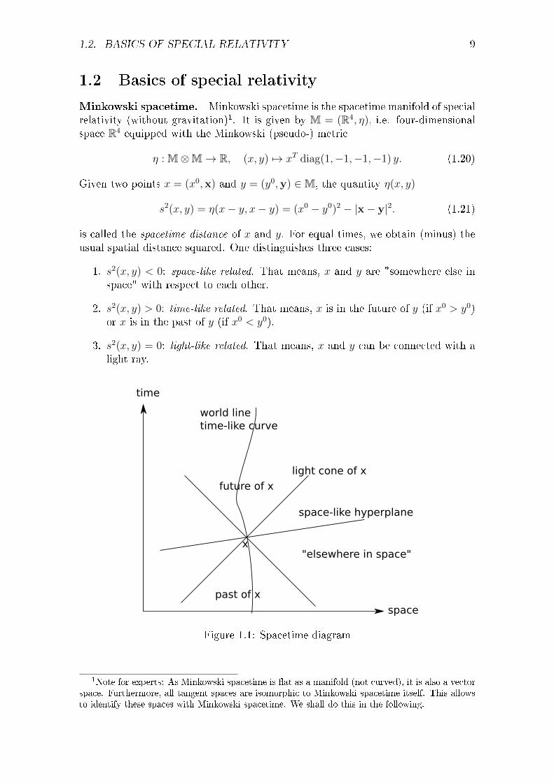
1.2 Basics of special relativity
Minkowski spacetime. Minkowski spacetime is the spacetime manifold of specialrelativity (without gravitation)1. It is given by M = (R4, η), i.e. four-dimensionalspace R4 equipped with the Minkowski (pseudo-) metric
η : M⊗M→ R, (x, y) 7→ xT diag(1,−1,−1,−1) y. (1.20)
Given two points x = (x0,x) and y = (y0,y) ∈M, the quantity η(x, y)
s2(x, y) = η(x− y, x− y) = (x0 − y0)2 − |x− y|2. (1.21)
is called the spacetime distance of x and y. For equal times, we obtain (minus) theusual spatial distance squared. One distinguishes three cases:
1. s2(x, y) < 0: space-like related. That means, x and y are "somewhere else inspace" with respect to each other.
2. s2(x, y) > 0: time-like related. That means, x is in the future of y (if x0 > y0)or x is in the past of y (if x0 < y0).
3. s2(x, y) = 0: light-like related. That means, x and y can be connected with alight ray.
world linetime-like curve
light cone of x
space-like hyperplane
"elsewhere in space"x
past of x
future of x
space
time
Figure 1.1: Spacetime diagram
1Note for experts: As Minkowski spacetime is at as a manifold (not curved), it is also a vectorspace. Furthermore, all tangent spaces are isomorphic to Minkowski spacetime itself. This allowsto identify these spaces with Minkowski spacetime. We shall do this in the following.
10 CHAPTER 1. BACKGROUND
Index notation. We set ~ = c = 1.We denote vectors x ∈ M by x = (x0, x1, x2, x3). xµ, µ = 0, 1, 2, 3 are the com-ponents of x in a particular inertial frame. The component x0 = ct correspondsto time, and the spatial components are often indicated by using roman indices xj,j = 1, 2, 3. We sometimes write x = (t,x) with x ∈ R3.Covectors ω ∈M∗ are maps ω : M→ R. We denote them using lower indices
ω = (ωµ)µ=0,1,2,3. (1.22)
Their action on a vector x is given by
ω x =3∑
µ=0
ωµxµ. (1.23)
We also abbreviate this by
ωµxµ =
3∑µ=0
ωµxµ, (1.24)
where summation over the repeated upper and lower index µ is implied. This iscalled a contraction of the index µ.Vector elds A : M→M are given by
A(x) = (Aµ(x)) = (A0(x), ..., A3(x)). (1.25)
Tensor elds of order (m,n) are dened as maps T : M→ (M⊗ · · ·M︸ ︷︷ ︸m
)⊗(M∗ ⊗ · · ·M∗︸ ︷︷ ︸n
)
and their components at a spacetime point x are denoted by
T µ1...µmν1...νn(x). (1.26)
Linear mapsM : M→M can be identied with constant tensor elds of order (1, 1)and their components are denoted by Mµ
ν . The action of M on a vector x is thenwritten as
(Mx)µ = Mµν x
ν . (1.27)
The composition of linear maps B,C is given as
(BC)µν = BµρC
ρν . (1.28)
Moreover, we have
Bνµ = (BT )µν . (1.29)
The transpose thus converts vector indices in covector indices and vice versa.Mµ
µ =∑3
µ=0Mµµ yields the trace of M (sum of diagonal elements).
The identity map is denoted by
I = (δµν) (1.30)
where δµν = 1 if µ = ν and δµν = 0 else.
1.2. BASICS OF SPECIAL RELATIVITY 11
The spacetime-metric should be seen as a (constant) tensor of order (0, 2). Thecomponents of the inverse of the metric, η−1, are denoted by ηµν (note the indexplacement!) and given by the relation
ηµρηρν = δµν . (1.31)
This leads to ηµν = ηµν , i.e., η and η−1 have the same components, apart from theindex placement.
Using ηµν and ηµν , we introduce the concept of raising and lowering indices. For
any vector with components xµ, we dene a corresponding covector with componentsxµ by:
xµ = ηµν xν . (1.32)
Concretely, if (xµ) = (x0, x1, x2, x3), then (xµ) = (x0,−x1,−x2,−x3).Similarly, for a covector with components yµ, we dene a corresponding vector withcomponents yµ by
yµ = ηµν yν . (1.33)
Concretely, if (yµ) = (y0, y1, y2, y3), then (yµ) = (y0,−y1,−y2,−y3).Similarly we dene the operators of raising/lowering indices for all tensors. Remem-ber: the index placement is important! It should be clear from the start which indexplacement an object should have.
Derivatives with respect to coordinates are denoted by
∂µ =∂
∂xµ(1.34)
and also here we use ∂µ = ηµν∂ν .Finally, the Minkowski square of a vector x ∈M is dened by:
x2 = xµxµ. (1.35)

12 CHAPTER 1. BACKGROUND
2. The Poincaré group
2.1 Lorentz transformations.
These are the symmetry transformations of Minkowski spacetime.
Denition: A Lorentz transformation is a map
Λ : M→M, x 7→ Λµν x
ν (2.1)
which preserves spacetime distances:
∀x, y ∈M : s2(Λx,Λy) = s2(x, y). (2.2)
This is equivalent to
∀x ∈M : η(Λx,Λx) = η(x, x). (2.3)
The set of all Lorentz transformations is denoted by L.
Denition: A real Lie group is a group G which is also a real, nite-dimensionalsmooth manifold. In addition, the group operations multiplication and inversion arerequired to be smooth maps from G×G→ G.
Theorem 2.1.1 L is a 6-dimensional Lie group. It is often called L = O(3, 1).
Proof: → Sheet 2, Exercise 1
Examples.
1. Rotations. Let R ∈ SO(3) be a rotation. SO(3) is the group of orthogo-nal real 3 × 3 matrices with determinant equal to 1. This denes a Lorentztransformation by leaving the time coordinate unchanged:
Λ =
(1 0T
0 R
). (2.4)
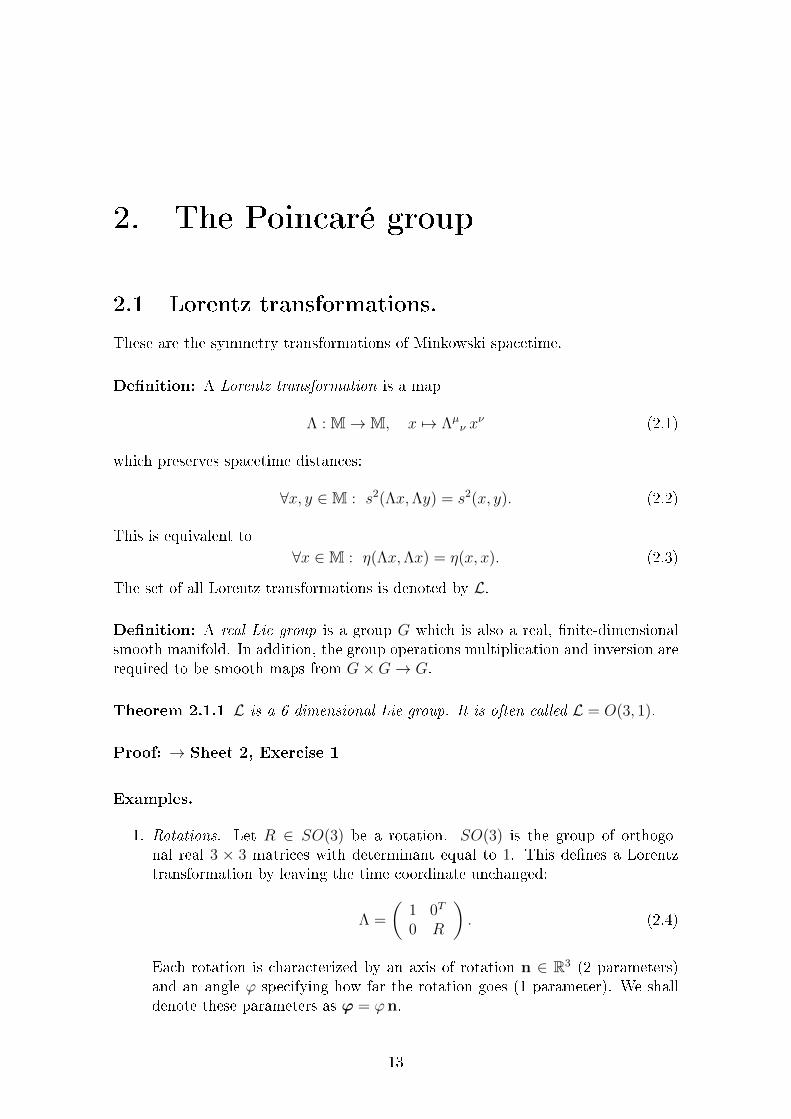
Each rotation is characterized by an axis of rotation n ∈ R3 (2 parameters)and an angle ϕ specifying how far the rotation goes (1 parameter). We shalldenote these parameters as ϕ = ϕn.
13
14 CHAPTER 2. THE POINCARÉ GROUP
2. Boosts. These describe the transition from the old frame to another movingwith velocity v (v = |v| < 1) with respect to the former. Let
γ(v) =1√
1− v2. (2.5)
Then the boost is given by
Λ =
(γ(v) γ(v)vT
γ(v)v 13 + γ(v)−1v2 vvT
). (2.6)
Note: v should be regarded as a column vector, and (vvT )ij = vivj. If weparametrize v as
v = tanh(ω)v/|v|, ω ∈ [0,∞) (2.7)
then every Lorentz boost is characterized by the boost vector
ω = ω v/|v| ∈ R3. (2.8)
3. Discrete transformations. In addition, there are also the space inversion P("parity"), the time reversal T and the combination of both, PT .
P =
(1 0T
0 −13
),
(−1 0T
0 13
), PT = −14. (2.9)
Remark. The Lorentz group consists of the following four connected components:
L↑+ = Λ ∈ L|Λ00 ≥ 1, det Λ = +1,
L↑− = Λ ∈ L|Λ00 ≥ 1, det Λ = −1 = PL↑+,
L↓− = Λ ∈ L|Λ00 ≤ −1, det Λ = −1 = TL↑+,
L↓+ = Λ ∈ L|Λ00 ≤ −1, det Λ = +1 = PTL↑+. (2.10)
The discrete transformations thus relate the connected components of L to eachother. L↑+ is called the proper Lorentz group and is itself a Lie group.
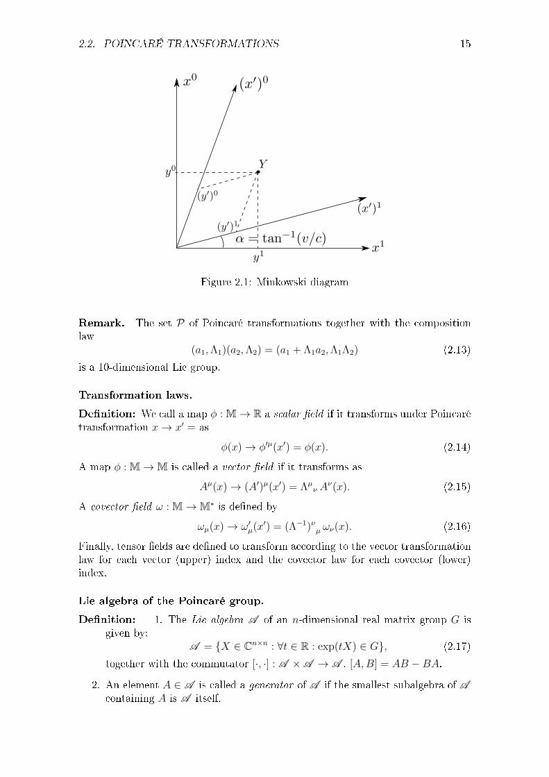
Visualization of Lorentz boosts: Minkowski diagrams. A boost in x1 direc-tion is given by (c = 1):
(x′)0 = γ(v)(x0− vx1), (x′)1 = γ(v)(x1− vx0), , (x′)2 = x2, (x′)3 = x3. (2.11)
This change of coordinates can be represented graphically in Minkowski diagrams(see Fig. 2.1).
2.2 Poincaré transformations
Denition: A Poincaré transformation Π = (a,Λ) with a ∈M and Λ ∈ L is a mapM→M dened by
Πx = a+ Λx. (2.12)
2.2. POINCARÉ TRANSFORMATIONS 15
Figure 2.1: Minkowski diagram
Remark. The set P of Poincaré transformations together with the compositionlaw
(a1,Λ1)(a2,Λ2) = (a1 + Λ1a2,Λ1Λ2) (2.13)
is a 10-dimensional Lie group.
Transformation laws.
Denition: We call a map φ : M→ R a scalar eld if it transforms under Poincarétransformation x→ x′ = as
φ(x)→ φ′µ(x′) = φ(x). (2.14)
A map φ : M→M is called a vector eld if it transforms as
Aµ(x)→ (A′)µ(x′) = Λµν A
ν(x). (2.15)
A covector eld ω : M→M∗ is dened by
ωµ(x)→ ω′µ(x′) = (Λ−1)νµ ων(x). (2.16)
Finally, tensor elds are dened to transform according to the vector transformationlaw for each vector (upper) index and the covector law for each covector (lower)index.
Lie algebra of the Poincaré group.
Denition: 1. The Lie algebra A of an n-dimensional real matrix group G isgiven by:
A = X ∈ Cn×n : ∀t ∈ R : exp(tX) ∈ G, (2.17)
together with the commutator [·, ·] : A ×A → A , [A,B] = AB −BA.
2. An element A ∈ A is called a generator of A if the smallest subalgebra of Acontaining A is A itself.
16 CHAPTER 2. THE POINCARÉ GROUP
Generators of the Poincaré group. P is a 10-dimensional Lie group, so we canintroduce coordinates in R10 such that the identity element e corresponds to theorigin, and every other element in a neighborhood of e is characterized by
q = (a,ω,ϕ) ∈ R10. (2.18)
Choosing a as the translation vector, ω as the boost parameter and ϕ as the rotationparameter, the coordinate lines qj(t) = (0, ...., t, ...., 0) (j-th place) are one-parametersubgroups of the proper Poincaré group
P↑+ = (a,Λ) ∈ P : Λ ∈ L↑+ (2.19)
such that group multiplication is given by adding the parameters as in
qj(s) qj(t) = qj(s+ t). (2.20)
One obtains 10 one-parameter subgroups in this way. Their innitesimal generatorsAj are dened by
Aj =d
dtqj(t)
∣∣∣∣t=0
(2.21)
and denoted as follows:
−p0 = −H0 generator of x0-translations,p1, p2, p3 generators of x1, x2, x3-translations,−N1,−N2,−N3 generators of boosts in x1, x2, x3-directions,J1, J2, J3 generators of rotations around the x1, x2, x3-axes.
Their Lie algebra is given by:
[pj, pk] = 0 = [pj, H0] = [Jj, H0],[Nj, pk] = −δjkH0, [Nj, H0] = pj,[Jj, pk] = −
∑m εjkmpm [Jj, Jk] = −
∑m εjkmJm,
[Nj, Nk] =∑
m εjkmJm [Jj, Nk] = −∑
m εjkmNm.
Note: The last three equations form the Lie algebra of the Lorentz group.
Index notation for generators. We can conveniently summarize the PoincaréLie algebra as follows. Let
M j0 = Nj, j = 1, 2, 3, M12 = J3, M13 = J2, M23 = J1 (2.22)
and dene Mνµ = −Mµν , µν = 0, 1, 2, 3. Then the Poincaré Lie algebra is given by:
[Mµν , pσ] = i(ηνσpµ − ηµσpν), (2.23)
[pµ, pν ] = 0 (2.24)
and[Mµν ,Mρσ] = −i(ηµρMνσ − ηνρMµσ + ηµσMρν − ηνσMρµ). (2.25)
Exponentiating the Lie algebra. We obtain the proper Poincaré group P↑+through exponentiation as
P↑+ = exp(ipµaµ) exp(ωµνM
µν/2) : aµR ∀µ, ωµν ∈ R, ωµν = −ωνµ ∀µ, ν. (2.26)
2.3. INVARIANCE OF WAVE EQUATIONS 17
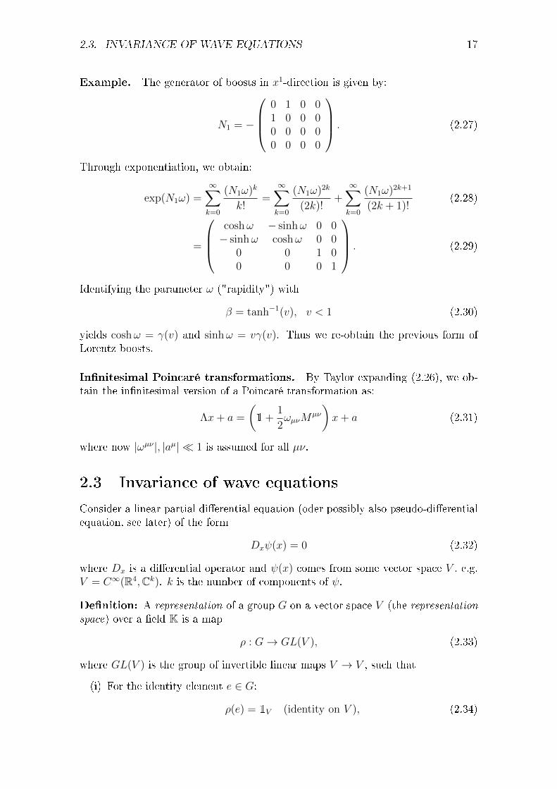
Example. The generator of boosts in x1-direction is given by:
N1 = −
0 1 0 01 0 0 00 0 0 00 0 0 0
. (2.27)
Through exponentiation, we obtain:
exp(N1ω) =∞∑k=0
(N1ω)k
k!=∞∑k=0
(N1ω)2k
(2k)!+∞∑k=0
(N1ω)2k+1
(2k + 1)!(2.28)
=
coshω − sinhω 0 0− sinhω coshω 0 0
0 0 1 00 0 0 1
. (2.29)
Identifying the parameter ω ("rapidity") with
β = tanh−1(v), v < 1 (2.30)
yields coshω = γ(v) and sinhω = vγ(v). Thus we re-obtain the previous form ofLorentz boosts.
Innitesimal Poincaré transformations. By Taylor expanding (2.26), we ob-tain the innitesimal version of a Poincaré transformation as:
Λx+ a =
(1+
1
2ωµνM
µν
)x+ a (2.31)
where now |ωµν |, |aµ| 1 is assumed for all µν.
2.3 Invariance of wave equations
Consider a linear partial dierential equation (oder possibly also pseudo-dierentialequation, see later) of the form
Dxψ(x) = 0 (2.32)
where Dx is a dierential operator and ψ(x) comes from some vector space V , e.g.V = C∞(R4,Ck). k is the number of components of ψ.
Denition: A representation of a group G on a vector space V (the representationspace) over a eld K is a map
ρ : G→ GL(V ), (2.33)
where GL(V ) is the group of invertible linear maps V → V , such that
(i) For the identity element e ∈ G:
ρ(e) = 1V (identity on V ), (2.34)
18 CHAPTER 2. THE POINCARÉ GROUP
(ii)ρ(g1g2) = ρ(g1)ρ(g2) ∀g1, g2 ∈ G. (2.35)
In the case that V is nite dimensional, we let n = dimV and identify GL(V ) withGL(n,K), the group of n × n invertible matrices on the eld K. In that case, wecall ρ a matrix representation.
If V is a complex vector space equipped with a scalar product 〈·, ·〉 then we callthe representation ρ unitary if all ρ(g) are unitary for all g ∈ G. (Similarly forantiunitary.)
If V is a Hilbert space and G a topological group, then we call ρ a Hilbert spacerepresentation if in addition to (i), (ii):
(iii) gn → g in G implies for all ψ ∈ V : ρ(gn)ψ → ρ(g)ψ (strong continuity).
Two representations ρ, π on V are said to be equivalent if there is an isomorphismφ : V → V such that for all g ∈ G:
φ ρ(g) φ−1 = π(g). (2.36)
Denition: Equation (2.32) is called invariant under a matrix representation ρ ofa group G on the representation space Ck if for every solution ψ of (2.32) and everyg ∈ G also the transformed wave function
ψ′(x′) = ρ(g)ψ(x) (2.37)
is a solution of (2.32) in the variables x′ = gx.
Remark. Invariance under a matrix representation is only a minimal requirement.Often additional requirements are appropriate, such as the invariance under a uni-tary representation. Furthermore, one often seeks a representation on a Hilbertspace instead of just a matrix representation. We shall discuss what kind of rep-resentation one can obtain case-by-case for the individual wave equations we shallstudy in the lecture.
2.4 Wish list for a relativistic wave equation
1. Linear partial dierential equation
2. Invariant under a representation of the Poincare group
3. Implies a continuity equation for a 4-current j = (ρ, j)
4. j is future-pointing and time-like, i.e. jµjµ > 0, j0 > 0,
5. j0 reduces to |ψ|2 in a suitable non-relativistic limit (or j0 = |ψ|2 in general)
6. The equation has propagation speed< 1, meaning that the support of solutionsgrows with at most the speed of light.
3. The Klein-Gordon equation
3.1 Derivation
Recall the quantization recipe for the Schrödinger equation. The idea was to takethe energy-momentum relation and to replace E and p by operators. This recipe isapplicable to the relativistic case as well. The relativistic energy-momentum relationreads
E =√
p2c2 +m2c4. (3.1)
Using the quantization recipe E → i~∂t and p → −i~∇ leads to the so-calledSalpeter equation
i~∂tψ(t,x) =√−∇2~2c2 +m2c4 ψ(t,x). (3.2)
This equation can be understood as a pseudo-dierential equation for scalar wavefunction ψ : M → C which are also square integrable (L2) with respect to x. Theidea is to use the Fourier transformation to dene what the operator
√p2c2 +m2c4
means, namely (denoting the spatial Fourier transformation of ψ with ψ):
√∇2~2c2 +m2c4 ψ(t,x) =
∫d3k
(2π)3eik·x√k2~2c2 +m2c4 ψ(t,k). (3.3)
The Fourier transformation implies that (3.2) has a non-local feature, meaning thatthe evaluation
√−∇2~2c2 +m2c4ψ(t,x) in a point (t,x) requires the knowledge of
ψ(t,k) for all k ∈ R3 (and thus of ψ(t,x) for all x). The Salpeter equation thusdoes not treat space and time on an equal level: the time derivative occurs as anordinary partial derivative while the spatial derivatives occur as a pseudo-dierentialoperator. It is, however, still possible to prove the relativistic invariance using thetrivial representation of the (proper) Poincaré group ρ(a,Λ) = 1 ∀(a, λ) ∈ P↑+, i.e.,with the transformation rule
ψ′(x′) = ψ(x). (3.4)
A major problem, though, is the fact that |ψ|2 cannot be the 0-component of acurrent 4-vector that transforms in the right way. This is because then |ψ|2 wouldhave to transform as the component of a vector while in fact it transforms as a scalareld. (Note that this is a general point which does not depend on the particularwave equation under discussion.) Nevertheless, one can show (Sheet 3, Exercise1) that the integral P (t) =
∫d3x |ψ|2(t,x) does not depend on time.
Apart from this, (3.2) has an innite propagation speed (not a propagation speedof at most the speed of light), meaning that after a small time t > a compactly sup-ported wave function ψ(t, ·) can have support all over space. For these reasons,
19

20 CHAPTER 3. THE KLEIN-GORDON EQUATION
one usually rejects the Salpeter equation as a relativistic quantum mechanical waveequation.
An obvious way to avoid the pseudo-dierential equation (3.2) is to take thesquare of the energy momentum relation,
E2 = p2c2 +m2c4 (3.5)
and to only then apply the quantization recipe. This leads to the Klein-Gordon(KG) equation:
− ∂2t ~2ψ(t,x) = (−∇2~2c2 +m2c4)ψ(t,x). (3.6)
A more compact way of writing the equation is (after dividing by c2~2):( +
m2c2
~2
)ψ(t,x) = 0 (3.7)
where
=1
c2
∂2
∂t2−∆ (3.8)
is the d'Alembertian (also called "wave operator").In index notation, the KG equation can also be expressed as(
∂µ∂µ +
m2c2
~2
)ψ(t,x) = 0. (3.9)
From now on, we shall again set ~ = 1 = c.
3.2 Physical properties
Relativistic invariance.
Theorem 3.2.1 The KG equation is invariant under the trivial representation ofthe Poincaré group
ρ(g) = 1 ∀g ∈ P . (3.10)
The proof is an immediate consequence of Sheet 2, Exercise 1 where you willshow that ∂µ∂
µf transforms, for every scalar function f : M→ C, as a scalar underLorentz transformations Λ : x 7→ x′ = Λx, meaning that
∂′µ∂µ′φ′(x′) = ∂µ∂
µφ(x). (3.11)
For a Poincaré transformation (a,Λ) : x 7→ x′ = Λx+a, the transformation behavioris the same as the operator ∂µ is invariant under translations. Moreover, the massterm transforms by denition as
m2φ′(x′) = m2φ(x). (3.12)
Thus, the whole KG equation is Poincaré invariant.
3.2. PHYSICAL PROPERTIES 21
Plane wave solutions. We make the ansatz
φ(x) = e−ikµxµ
(3.13)
where k0 = E. Inserting (3.13) into the KG equation yields
(−k2 +m2)e−ikµxµ
= 0. (3.14)
Hence we obtain a plane-wave solution if the following dispersion relation holds:
k2 = m2 ⇔ (k0)2 (= E2) = k2 +m2. (3.15)
Letω(k) =
√k2 +m2. (3.16)
At this point, we see an important feature of the KG equation: For every k ∈ R3,both E = +ω(k) and E = −ω(k) lead to a plane-wave solution. The meaningof negative energies is unclear at this point. It is certainly something one it notused to from classical physics or from non-relativistic QM where the Hamiltonianis bounded from below so that one can make all energies positive by addition ofa constant. If this is not the case, one might for example worry that the systemcould lower its energy indenitely by emitting radiation (which does not happenin nature). However, these are just worries which are based on an intuition comesfrom equations dierent from the KG equation. We have to analyze the KG equationdeeper to see whether negative energies are really problematic.
For the moment, we note that for φ+, φ− ∈ C(R3,C) ∩ L2(R3,C) we obtain alarge class of solutions of the KG equation by (inverse) Fourier transformation as:
ψ(x) =
∫d3k
(2π)3
(eik·x−iω(k)x0
φ+(k) + eik·x−iω(k)x0
φ−(k)). (3.17)
Conserved current. One can check (Sheet 3, Exercise 2) that for every dif-ferentiable solution ψ(x) of the KG equation the current
jµ(x) = Im (ψ(x)∂µψ∗(x)) (3.18)
is conserved, meaning∂µj
µ(x) = 0. (3.19)
Furthermore, it follows from Sheet 2, Exercise 1 that j transforms under Poincarétransformations as a vector eld, i.e.
j′µ(x′) = Λµνjν(x). (3.20)
However, there is a disturbing property of the density component
ρ(t,x) = j0(t,x) = Im (ψ(t,x)∂tψ∗(t,x)) , (3.21)
namely ρ(t,x) can become negative for certain wave functions ψ(t,x). Forexample, consider a plane wave solution with negative energy E = −ω(k) for somek ∈ R3:
ψ(t,x) = eik·x+iω(k)t. (3.22)
22 CHAPTER 3. THE KLEIN-GORDON EQUATION
Then:
ρ(t,x) = Im(eik·x+iω(k)t∂te
−ik·x−iω(k)t)
= Im(eik·x+iω(k)t(−iω(k))e−ik·x−iω(k)t
)= −ω(k) < 0. (3.23)
Note that we cannot remove this problem by changing the overall sign of j as thena positive energy plane wave would lead to ρ(t,x) < 0. Thus ρ cannot play therole of a probability density. The physical interpretation of the KG equationis thus unclear. The source of the problem is the occurrence of both positive andnegative energies.
Restriction to positive energies. In view of the above situation, it looks likea logical step to try to restrict oneself to positive energies. That means, we onlyadmit solutions of the form
ψ(x) =
∫d3k
(2π)3eik·x−iω(k)x0
φ+(k). (3.24)
for some function φ+ ∈ L2(R3). Such a ψ(t,x) also solves the Salpeter equation.We call the vector space of solutions of the form (3.24) Vpos.
The situation can then be summarized as follows.
1. The "total probability integral"
P (Σ) =
∫Σ
dσµ(x) Im(ψ(x)∂µψ∗(x)) (3.25)
is, for every space-like hyperplane Σ ⊂ M, positive and independent of Σ.(This can be seen by rst specializing to the case of Σ = Σt = (t,x) ∈ M :t = const and using (3.24). In a second step one can then employ the result ofExercise 3, Sheet 2 to show that the result holds for all space-like hyperplanesΣ. → Sheet 3, Exercise 2.)
2. Nevertheless, jµ(x) = Im(ψ(x)∂µψ∗(x)) can be space-like for certain wavefunctions ψ.1
3. The restriction to positive energies does not work anymore if one includes anexternal potential in the KG equation. This would be done (according to thequantization recipe) as:
(Ekin +V )2 = p2 + m2 → (−∂t+V )2ψ(t,x) = (−∇2 +m2)ψ(t,x). (3.26)
A potential can then cause transitions from positive to negative energies.
Overall, a probabilistic interpretation of the KG equation is thus problematic, andwe shall later look for a dierent wave equation. However, as the KG equation is stillused as a toy example (and also as an ingredient for some quantum eld theories),we shall now study its mathematical theory rst.
1See R. Tumulka, J. Phys. A: Math. Gen. 35 (2002) 7961-7962, https://arxiv.org/abs/quant-ph/0202140. → Sheet 3, Exercise 2.

3.3. SOLUTION THEORY 23
3.3 Solution theory
Green's function method for the initial boundary value problem. Wefollow Zauderer2. For a bounded region G ⊂ R3 and the time interval [0, T ], wewould like to solve the boundary initial value problem
ψ(0,x) = f(x), x ∈ G,∂tψ(0,x) = g(x), x ∈ G,ψ(t,x) = B(t,x), x ∈ ∂G, t ∈ [0, T ]( +m2)ψ(t,x) = 0, x ∈ G, t ∈ [0, T ].
(3.27)
Here, f, g and B are given functions. We may (where necessary) assume them tobe smooth in order to avoid technical complications. Note that in (3.27) we haveto prescribe ∂tψ0, ·) in addition to ψ(0, ·). This is because the KG equation is ofsecond order.
Here we consider a bounded region as an intermediary step. The result forunbounded regions is obtained in a suitable limit. The exact form of the boundaryconditions then does not matter. Here we we chose Dirichlet boundary conditions.
The idea is to use an integral theorem for a cleverly chosen combination offunctions as well as for the spacetime region
R = G× [0, T ] (3.28)
for some T > 0. The boundary of R has the form
∂R = ∂R0 ∪ ∂RT ∪ ∂Rx (3.29)
where ∂R0 = (t,x) ∈ ∂R : t = 0, ∂RT = (t,x) ∈ ∂R : t = T and ∂Rx =(t,x) ∈ ∂R : x ∈ ∂G. The exterior unit normal vector n at ∂R has the formn = (−1,0) on ∂R0, n = (1,0) on ∂RT and n = (0,nx) on ∂Rx.
We furthermore write the KG equation as
∂2t ψ(t,x) = −(−∆ +m2)ψ(t,x) =: −Lψ(t,x). (3.30)
Now we come to the integral identity. For arbitrary dierentiable functionsu(t,x), w(t,x) we have,
∂µ(w∂µu− u∂µw) = (∂µw)(∂µu) + wu− (∂µu)(∂µw)− uw = wu− uw= w∂2
t u− w∆u− w∂2t u+ u∆w − wm2u+ um2w
= w(∂2t u+ Lu)− u(∂2
tw + Lw). (3.31)
Therefore we nd, using the 4-dimensional divergence theorem applied to the vectoreld w∂µu− u∂µw:∫
R
dt d3x [w((∂2t u) + Lu)− u((∂2
tw) + Lw)] =
∫∂R
dσ nµ(w∂µu− u∂µw). (3.32)
2E. Zauderer, Partial Dierential Equations of Applied Mathematics, Wiley 2006, pp. 412
24 CHAPTER 3. THE KLEIN-GORDON EQUATION
Here we have:∫∂R
dσ nµ(w∂µu− u∂µw)
=
∫∂Rx
dσ (−w∇u+ u∇w) · n +
∫∂RT
dσ (w∂tu− u∂tw)−∫∂R0
dσ (w∂tu− u∂tw).
(3.33)
The idea of the Green's function method now is to choose a particular function wsuch that u(τ,y) can be determined from (3.33) at a particular point (τ,y) ∈ R.It turns out that w will then in general be a generalized function (distribution).The following manipulations will therefore only be of formal nature, and we have tocheck in the end whether we really obtain a sensible solution. We require:
∂2tw(t,x) + Lw(t,x) = δ(t− τ)δ(3)(x− y). (3.34)
Then: ∫R
d4xu(∂2tw + Lw) =
∫R
d4xu δ(t− τ)δ(3)(x− y) = u(τ,y). (3.35)
For a solution u of the KG equation we have:∫R
d4xw(∂2t u+ Lu) = 0, (3.36)
so the l.h.s. of (3.32) reduces to u(τ,y). We now work at simplifying the r.h.s.Furthermore, we have:∫
∂Rx
dσ (−w∇u+ u∇w) · n =
∫∂Rx
dσ
(−w∂u
∂n+ u
∂w
∂n
). (3.37)
Thus, if we requirew(t,x)|∂Rx
= 0 (3.38)
then we nd, using both the boundary conditions for w (= 0) and u (= B):∫∂Rx
dσ
(−w∂u
∂n+ u
∂w
∂n
)=
∫∂Rx
dσ B∂w
∂n. (3.39)
Here, ∂w∂n
= n · ∇w denotes the normal derivative of w (in the spatial directions).In order to determine w completely, we expect that initial conditions for w and
wt must be prescribed for some t. As we want to utilize (3.33) as best as possible,we have to examine at which time it makes most sense to prescribe the initialconditions. We want to do this in a way such that the r.h.s. of (3.33) does notcontain any unkown functions. Considering the terms on the r.h.s. of (3.33), wehave two possible choices: t = 0 or t = T . If we prescribe w and ∂tw for t = 0, thenthe second term in (3.33) still contains u(t,x) and ∂tu(tx) for t = T . However, ifwe prescribe w and ∂tw for t = T as
w(T, ·) = 0, ∂tw(T, ·) = 0 (3.40)
3.3. SOLUTION THEORY 25
then the r.h.s. of (3.33) only contains the initial data and boundary values for u.So this is a distinguished choice, and we shall make it. The function w dened bythe conditions (3.34), (3.38) and (3.40) is called the Green's function for the initialboundary value problem, and it is denoted by
K(t,x; τ,y) = w(t,x). (3.41)
Given a distribution which satises these conditions (it may not always exist), weobtain the solution u(τ,y) through the formula (3.33) as:
u(τ,y) =
∫∂R0
dσ (Kg − (∂tK)f)−∫∂Rx
dσ B∂K
∂n(3.42)
This useful formula gives a solution of the initial boundary value problem, providedthe integrals exist (and are of the desired regularity). We will prove this later.
Unbounded domains. We would like to consider the unbounded spatial domainR3. We achieve this by considering R = Br(0) and letting r →∞ in (3.42). This ispossible only if the integral∫
∂R0
dσ (Kg −Ktf) =
∫Br(0)
d3x (K(0,x; τ,y)g(x) + (∂tK)(0,x; τ,y)f(x)) (3.43)
exists in the limit r → ∞. The second integral in (3.42) can be made identicallyzero by choosing B = 0. Then we have:
u(τ,y) =
∫d3x (K(0,x; τ,y)g(x)− (∂tK)(0,x; τ,y)f(x)) . (3.44)
Green's function of the KG equation. It is quite some work to calculatethe Green's function of the KG equation. A systematic way is to use the Fouriertransformation (taking into account the boundary conditions). Another way is tomake a suitable ansatz for K, e.g., that K is only a function of the spacetimedistance s2(t,x; t′,x′), and thereby reduce the problem to nding singular solutionsto an ODE. The result for K is:
K(t,x; t′,x′) =1
4π
δ(t′ − t− |x′ − x|)|x′ − x|
− m
4πθ(t′ − t− |x′ − x|)
J1(m√
(t′ − t)2 − |x′ − x|2)√(t′ − t)2 − |x′ − x|2
. (3.45)
Here, J1 is a Bessel function of the rst kind. In general, we have for n ∈ N0:
Jn(x) =∞∑k=0
(−1)k
k!(k + n)!
(x2
)2k+n
(3.46)
Note thatJ1(x)
x=
1
2
∞∑k=0
(−1)k
k!(k + 1)!
(x2
)2k
(3.47)
26 CHAPTER 3. THE KLEIN-GORDON EQUATION
denes a smooth function on R.K can be written in terms of 4-vectors as:
K(x;x′) =1
2πθ(x′
0 − x0)δ((x′ − x)2)− m
4πθ(x′
0 − x0)θ((x′ − x)2)J1(m
√(x′ − x)2)√
(x′ − x)2
(3.48)where θ denotes the Heaviside step function.
The fact that K is a Green's function of the KG equation can be checked throughelementary (but lengthy) calculations. You may know already that
δ(t′ − t− |x− x′|)
4π|x′ − x|= δ(t′ − t)δ(3)(x′ − x), (3.49)
which, in turn, follows from ∆ 1|x′−x| = −4πδ(3)(x′ − x). Furthermore, one can show
that
−m
4πθ(t′ − t− |x− x′|)
J1(m√
(t′ − t)2 − |x′ − x|2)√(t′ − t)2 − |x′ − x|2
= −m2 δ(t′ − t− |x− x′|)
4π|x′ − x|+m3
4πθ(t′ − t− |x− x′|)
J1(m√
(t′ − t)2 − |x′ − x|2)√(t′ − t)2 − |x′ − x|2
.
(3.50)
To prove this, one uses (among other things) the identity
J1(m
√(t′ − t)2 − |x′ − x|2)√
(t′ − t)2 − |x′ − x|2= −m2J1(m
√(t′ − t)2 − |x′ − x|2)√
(t′ − t)2 − |x′ − x|2. (3.51)
From these identities it then follows thatK is a Green's function of the KG equation.The fact that K satises the initial data K(T,x; τ,y) = 0, ∂tK(T,x; τ,y) = 0 iseasy to see, as θ(t′−T −|x−x′|), δ(t′−T −|x−x′|) and δ′(t′−T −|x−x′|) vanishfor t ∈ (0, T ).
On Sheet 4, Exercise 1 you will prove a related statement, namely what theGreen's function of the 1+1 dimensional KG equation is.
The solution formula. Knowing the Green's function, we can now use (3.44) toexpress the solution of the Cauchy problem
ψ(0,x) = f(x), x ∈ R3,∂tψ(0,x) = g(x), x ∈ R3,( +m2)ψ(t,x) = 0, x ∈ R3, t ∈ [0, T ].
(3.52)
in terms of the initial data. In (3.44), we can write
−∫d3x (∂tK)(0,x; τ,y)f(x) = ∂τ
∫d3xK(0,x; τ,y)f(x) (3.53)
as K(t,x; τ,y) depends only on the dierence (t− τ,x− y). Thus, we obtain:
3.3. SOLUTION THEORY 27
u(τ,y)
=
∫d3x
(1
4π
δ(τ − |y − x|)|y − x|
g(x)− m
4πθ(τ − |y − x|)
J1(m√τ 2 − |y − x|2)√
τ 2 − |y − x|2g(x)
)
+∂
∂τ
∫d3x
(1
4π
δ(τ − |y − x|)|y − x|
f(x)− m
4πθ(τ − |y − x|)
J1(m√τ 2 − |y − x|2)√
τ 2 − |y − x|2f(x)
)(3.54)
We can simplify this result using spherical coordinates d3x = r2dr dΩx. The resultis:
u(τ,y) =τ
4π
∫∂Bτ (0)
dΩx g(x + y)− m
4π
∫Bτ (0)
d3xJ1(m
√τ 2 − |x|2)√
τ 2 − |x|2g(x + y)
+∂
∂τ
(τ
4π
∫∂Bτ (0)
dΩx f(x + y)− m
4π
∫Bτ (0)
d3xJ1(m
√τ 2 − |x|2)√
τ 2 − |x|2f(x + y)
).
(3.55)
Here, Bτ (0) ⊂ R3 is the ball with radius τ around the origin.
An important fact about the formula (3.55) is that it only contains integrationsof smooth functions over bounded regions. We shall use this fact to check that itindeed yields a solution of the Cauchy problem of the KG equation.
Theorem 3.3.1 Let f ∈ C3(R3) and g ∈ C2(R3). Then the function u : M → Cdened by (3.55) lies in C2(R4) and it solves the Cauchy problem (3.52).
Proof: C2 property. u ∈ C2(R) as it is dened by integrals involving only f, g andthe smooth function J1(x)/x over bounded domains.Initial data. To see what u(0,x) is, we take the limit τ → 0 in (3.55). The twointegrals in the rst line go to zero as the integrands are continuous functions andas such have an upper bound, say on B1(0). Similarly, in the second line, the onlysurviving term is
1
4π
∫∂Bτ (0)
dΩx f(y + x)→ f(x) for τ → 0, (3.56)
as it should be. For ∂τu(0,x), only the rst term in (3.55) contributes, namely:
∂ττ
4π
∫∂Bτ (0)
dΩx g(y + x) =1
4π
∫∂Bτ (0)
dΩx g(y + x) +τ
4π∂τ
∫|n|=1
d2n g(y + τn)
=1
4π
∫∂Bτ (0)
dΩx g(y + x) +τ
4π
∫|n|=1
d2n n · ∇g(y + τn)︸ ︷︷ ︸bounded
τ→0−→ g(y) + 0. (3.57)
28 CHAPTER 3. THE KLEIN-GORDON EQUATION
So the initial conditions are satised.Solution of the KG equation. Our strategy will be as follows: We rst show that theterms without mass, i.e.
u1(τ,y) =τ
4π
∫∂Bτ (0)
dΩx g(x + y)︸ ︷︷ ︸=:u
(g)1 (τ,y)
+∂
∂τ
τ
4π
∫∂Bτ (0)
dΩx f(x + y)︸ ︷︷ ︸=:u
(f)1 (τ,y)
(3.58)
satisfy the wave equation ∂2τu1(τ,y) = ∆u1(τ,y). Then we show that the terms
with mass, i.e.
u2(τ,y) = −m4π
∫Bτ (0)
d3xJ1(m
√τ 2 − |x|2)√
τ 2 − |x|2g(x + y)︸ ︷︷ ︸
=:u(g)2 (τ,y)
− ∂
∂τ
m
4π
∫Bτ (0)
d3xJ1(m
√τ 2 − |x|2)√
τ 2 − |x|2f(x + y)︸ ︷︷ ︸
=:u(f)2 (τ,y)
(3.59)satisfy
(∂2τ −∆)u2(τ,y) = −m2 (u1(τ,y) + u2(τ,y)) . (3.60)
This implies that u = u1 + u2 solves the KG equation.We start with ∂2
τu1(τ,y) = ∆u1(τ,y). As f and g can be chosen independently(and in particular one equal to zero), we treat the terms involving them separately.We have:
∂
∂τu
(g)1 (τ,y) =
1
4π
∫∂Bτ (0)
dΩx g(x + y) +τ
4π
∂
∂τ
∫|n=1|
d2n g(τn + y)
=1
4π
∫∂Bτ (0)
dΩx g(x + y) +τ
4π
∫|n=1|
d2nn · ∇g(τn + y)
=1
4π
∫∂Bτ (0)
dΩx g(x + y) +1
4πτ
∫Bτ (0)
d3x∆g(x + y) (3.61)
Here, we have used the divergence theorem for the transition to the last line. Thus,
∂2
∂τ 2u
(g)1 (τ,y)
=1
4π
∫|n=1|
d2nn · ∇g(τn + y)− 1
4πτ 2
∫Bτ (0)
d3x∆g(x + y) +1
4πτ
∂
∂τ
∫Bτ (0)
d3x∆g(x + y)
=1
4πτ 2
∫Bτ (0)
d3x∆g(x + y)− 1
4πτ 2
∫Bτ (0)
d3x∆g(x + y) +1
4πτ
∂
∂τ
∫Bτ (0)
d3x∆g(x + y)
=1
4πτ
∂
∂τ
∫Bτ (0)
d3x∆g(x + y). (3.62)
On the other hand,
∆u(g)1 (τ,y) =
τ
4π
∫∂Bτ (0)
dΩx ∆g(x + y) =1
4πτ
∫∂Bτ (0)
dσx ∆g(x + y)
=1
4πτ
∂
∂τ
∫Bτ (0)
d3x∆g(x + y). (3.63)
3.3. SOLUTION THEORY 29
Here we have used the identity
∂
∂τ
∫Bτ (0)
d3xh(x) =
∫∂Bτ (0)
dσx h(x). (3.64)
Thus, the g-part of u1 solves the wave equation. For the f -part one can proceedanalogously as we can interchange ∂2
τ and ∆ with the overall ∂τ -derivative, and asthe term otherwise has exactly the same form as the g-term. We have obtained theresult that u1 indeed solves the wave equation.
Next, we turn to the proof of the identity (3.60), u2 = −m2(u1 +u2). We againtreat the parts of u2 involving f and g separately. We start with the g-part. Theresult for the f -part can then be obtained analogously. We have:
∂
∂τu
(g)2 (τ,y) = −m
4π
∂
∂τ
∫ τ
0
dt t2∫d2n
J1(m√τ 2 − t2)√
τ 2 − t2g(tn + y)
= −m4πτ 2
∫d2n
(J1(m
√τ 2 − t2)√
τ 2 − t2
)tτ︸ ︷︷ ︸
=m/2
g(τn + y)
− m
4π
∫ τ
0
dt t2∫d2n ∂τ
(J1(m
√τ 2 − t2)√
τ 2 − t2
)g(tn + y). (3.65)
Taking another τ -derivative yields:
∂2τu
(g)2 (τ,y) =− m2τ
4π
∫∂Bτ (0)
dΩx g(x + y) (3.66)
− m2τ 2
8π
∫∂Bτ (0)
dΩx∂g
∂n(x + y) (3.67)
− mτ 2
4π
∫∂Bτ (0)
dΩx ∂τ
(J1(m
√τ 2 − t2)√
τ 2 − t2
)tτ︸ ︷︷ ︸
=−m3τ/8
g(x + y) (3.68)
− m
4π
∫Bτ (0)
d3x ∂2τ
(J1(m
√τ 2 − x2)√
τ 2 − x2
)g(x + y). (3.69)
This is to be compared with
∆yu(g)2 (τ,y) = −m
4π
∫Bτ (0)
d3xJ1(m
√τ 2 − x2)√
τ 2 − x2∆g(x + y). (3.70)
To bring this closer to the terms we obtained for ∂2τu
(g)2 (τ,y), we make use of the
second Green's identity∫V
d3xφ∆ψ =
∫V
d3xψ∆φ+
∫∂V
dσ
(φ∂ψ
∂n− ψ∂φ
∂n
). (3.71)
30 CHAPTER 3. THE KLEIN-GORDON EQUATION
This yields:
−m4π
∫Bτ (0)
d3xJ1(m
√τ 2 − x2)√
τ 2 − x2∆g(x + y)
= −m4π
∫Bτ (0)
d3x∆x
(J1(m
√τ 2 − x2)√
τ 2 − x2
)g(x + y) (3.72)
− m
4π
∫∂Bτ (0)
dσJ1(m
√τ 2 − x2)√
τ 2 − x2n · ∇xg(x + y) (3.73)
+m
4π
∫∂Bτ (0)
dσ n · ∇x
(J1(m
√τ 2 − x2)√
τ 2 − x2
)g(x + y). (3.74)
Next, we nd that (3.73) agrees with (3.67) because on ∂Bτ (0), we have x2 = τ 2
and
lim|x|→τ
J1(m√τ 2 − x2)√
τ 2 − x2=m
2. (3.75)
Similarly, (3.74) agrees with (3.68) on ∂Bτ (0), n = x/|x| and
limx2→τ2
x
|x|· ∇x
J1(m√τ 2 − x2)√
τ 2 − x2=m3τ
8, (3.76)
as one nds after a short calculation with Bessel functions (e.g. using the deningpower series).
Thus:
(∂2τ −∆y) =: u
(g)2 (τ,y) = (3.66) + (3.67)− (3.72)
= −m2τ
4π
∫∂Bτ (0)
dΩx g(x + y)− m
4π
∫Bτ (0)
d3x (∂2τ −∆x)
(J1(m
√τ 2 − x2)√
τ 2 − x2
)g(x + y).
(3.77)
Now, we have (as one can show after some calculations with Bessel functions):
(∂2τ −∆x)
(J1(m
√τ 2 − x2)√
τ 2 − x2
)= −m2
(J1(m
√τ 2 − x2)√
τ 2 − x2
), τ 2 > x2. (3.78)
Identifying also u(g)1 (τ,y) = − τ
4π
∫∂Bτ (0)
dΩx g(x + y), the conclusion is that
(∂2τ −∆y)u
(g)2 = −m2(u
(g)1 + u
(g)2 ). (3.79)
Hence, together with the previous result (∂2τ − ∆y)u
(g)1 = 0, we obtain that u(g) =
u(g)1 + u
(g)2 satises the KG equation. The same procedure can be used to show that
u(f) = u(f)1 + u
(f)2 solves the KG equation as well. Thus u = u(g) + u(f) is indeed a
solution of the KG equation.
Uniqueness of the solution. Next, we show that the solution formula (3.55)yields the only solution of the Cauchy problem (3.27). To this end, we use themethod of energy integrals (see e.g. Zauderer pp. 398).
3.3. SOLUTION THEORY 31
Theorem 3.3.2 Let u1, u2 ∈ C2([0, T ]×R3) be two solutions of the Cauchy problem(3.52) with ui(t, ·), ∂µui(t, ·), ∂µ∂νui(t, ·) ∈ L2(R3) for i = 1, 2, µ, ν = 0, 1, 2, 3 andall t ∈ [0, T ]. Then: u1 = u2.
Proof: Consider the "energy integral"
E(t) =1
2
∫d3x
[|∂tu|2 + |∇u|2 +m2|u|2
]. (3.80)
We will show that ddtE(t) = 0 for every solution u of the KG equation with the same
requirements as for u1, u2 in the theorem. Furthermore, we have E(t) ≥ 0∀t andE(t) = 0 ⇒ u(t, ·) = 0. Thus, if u(0, ·) = 0 then it follows that u(t, ·) = 0 ∀t. Foru = u1 − u2, we indeed have u(0, ·) = 0, as u1 and u2 satisfy the same initial data.Thus, u1(t, ·) = u2(t, ·)∀t ∈ [0, T ] follows.
We turn to the proof of ddtE(t) = 0. We have:
d
dtE(t) =
1
2
∫d3x
[(∂tu
∗)∂2t u+ (∇∂tu∗) · ∇u+m2(∂tu
∗)u]
+ c.c., (3.81)
where "c.c" denotes the complex conjugate of all the terms before. We would liketo bring this into a form where we can use that u satises the KG equation. To thisend, we need to rewrite the middle term. We have:
∇ · [(∂tu∗)∇u] = (∇∂tu∗) · ∇u+ ∂tu∗∆u. (3.82)
Hence (note that we need the integrability properties here):
d
dtE(t) =
1
2
∫d3x (∂tu
∗)(∂2t u−∆u+m2u) +
1
2
∫d3x∇ · [(∂tu∗)∇u] + c.c. (3.83)
Now we use that u is a solution of the KG equation, so the rst integral vanishes.We are left with
d
dtE(t) = lim
r→∞
1
2
∫Br(0)
d3x∇ · [(∂tu∗)∇u] + c.c.
= limr→∞
1
2
∫∂Br(0)
dσ n · [(∂tu∗)∇u] + c.c.
= 0, (3.84)
as ∂µu(t, ·) ∈ L2(R3)∀µ.
Remark. E can be written as the spatial integral over the 00-component of theenergy-momentum tensor of the KG equation:
T µν(x) =1
2
(∂νψ(x))∗(∂µψ(x)) + (∂µψ(x))∗(∂νψ(x))− ηµν
[(∂ρψ(x))∗(∂ρψ(x))−m2|ψ(x)|2
].
(3.85)Then T µν is real-valued and we have T µν = T νµ. Moreover, one can check (Sheet5, Exercise 4) that the KG equation implies
∂µTµν = 0 ∀ν = 0, 1, 2, 3. (3.86)
32 CHAPTER 3. THE KLEIN-GORDON EQUATION
Hence the integrals
P ν(Σ) =
∫Σ
dσ(x)nµ(x)T µν(x) (3.87)
are independent of the choice of the space-like hyperplane Σ. This is another way ofseeing that E(t) = P 0(Σt) does not depend on time. Note also that E cannot playthe role of total probability, as it transforms as the component of a vector underLorentz transformations.
Finite propagation speed.
Denition: We say that the KG equation has nite propagation speed if for allinitial data f ∈ C3(R3), g ∈ C2(R3) which are compactly supported in a ballBr(0) with radius r > 0, also the solution u(t, ·) and its rst derivative ∂tu(t, ·) arecompactly supported in a ball of radius r + |t|.
Corollary 3.3.3 The KG equation has nite propagation speed.
Proof: This can be read o from the solution formula (3.55) (using that it givesthe unique solution of the Cauchy problem (3.52). The detailed proof will be anexercise (Sheet 5, Exercise 1).
4. The Dirac equation
4.1 Derivation
This section largely follows Schweber1.The main problem of the Klein-Gordon equation is that the density component
of the current can become negative. One can see the reason for this behavior inthe fact that the current jµKG = Im(ψ∂µψ∗) contains derivatives. This, in turn, is aconsequence of the fact that the KG equation is of second order.
Therefore, Dirac's idea (1928) was that a relativistic quantum mechanical equa-tion should be of rst order, both in time and space derivatives. (The latter isunusual, as the Schrödinger equation contains second order spatial derivatives.) Hewrote down the general form of a linear equation which involves ψ as well as its timeand space derivatives. At the same time, he admitted that
ψ =
ψ1
ψ2...ψK
(4.1)
could have K complex-valued components. He arrived at the following general formof the equation (constants have been inserted with hindsight):
1
c
∂ψ
∂t+
3∑j=1
αj∂ψ
∂xj+imc
~βψ = 0. (4.2)
This is the general form of the Dirac equation. Here, α1, α2, α3 and β are constantcomplex K × K matrices. (Their constancy is required to obtain Poincaré invari-ance.) We still need to determine their possible form (and size K). Dirac did thisby imposing the following requirements (compare with our wish list):
1. Eq. (4.2) should imply that there is a spatial current j such that ρ = ψ†ψ =∑Kl=1 |ψl|2 and j satisfy the continuity equation. Then ρ could play the role of
a probability density.
2. Each component of ψ should satisfy the KG equation, as it implies the desiredenergy-momentum relation p2 = m2c2. (This should come out in some way insemi-classical situations, e.g. in scattering theory, and having it hold strictlyfor plane waves will ensure this.)
1S. Schweber: An Introduction to Relativistic Quantum Field Theory. Row Peterson andCompany, 1961, Chap. 4
33
34 CHAPTER 4. THE DIRAC EQUATION
So let us see what these requirements lead to. In order to calculate ∂tρ = ∂tψ†ψ,
it is useful to note down the Hermitian conjugate (complex conjugate and transpose)of (4.2).
1
c
∂ψ†
∂t+
3∑j=1
∂ψ†
∂xj(αj)† − imc
~ψ†β† = 0. (4.3)
Taking the time derivative of ρ = ψ†ψ then leads to:
1
c∂tψ
†ψ = −3∑j=1
(∂ψ†
∂xj(αj)†ψ + ψ†αj
∂ψ
∂xj
)− imc
~(ψ†βψ − ψ†β†ψ). (4.4)
We would like to write this as the divergence of something. That means, every termon the right hand side must contain a spatial derivative. Thus, the last term mustvanish. This leads to the condition
β† = β, (4.5)
i.e., β must be a Hermitian matrix. Then the remaining terms
−3∑j=1
(∂ψ†
∂xj(αj)†ψ + ψ†αj
∂ψ
∂xj
)(4.6)
can be written as the divergence
−3∑j=1
∂j(ψ†αjψ) (4.7)
if we also have(αj)∗ = αj, j = 1, 2, 3. (4.8)
Thus, we obtain the conserved 4-current
j = (ψ†ψ, cψ†αψ) (4.9)
where α = (α1, α2, α3) is the 3-vector of α-matrices.Now we have see what the second requirement amounts to. To this end, we let
the operator
1
c
∂
∂t−
3∑j=1
αj∂
∂xj− imc
~β (4.10)
act on (4.2). The idea behind this is to get second order derivatives into the equationwhich can then be compared with the KG equation. It is also somewhat analogousto decomposing a second order dierential operator into a product of rst orderdierential operators, such as the wave operator for 1+1 dimensions: ∂2
t − ∂2x =
(∂t − ∂x)(∂t + ∂x). Here we get
1
c2
∂2ψ
∂t2=
3∑j,k=1
1
2(αjαk+αkαj)
∂2ψ
∂xj∂xk−m
2c2
~2β2ψ+
imc
~
3∑j=1
(αjβ+βαj)∂ψ
∂xj. (4.11)
4.1. DERIVATION 35
In the rst term of the r.h.s., we have used the symmetric rewriting∑3
j,k=1 αjαk ∂2ψ
∂xj∂xk=∑3
j,k=112(αjαk + αkαj) ∂2ψ
∂xj∂xkwhich is possible for every ψ ∈ C2.
At this point, we can clearly see which conditions requirement 2 implies. Ther.h.s. of (4.11) reduces to∇2ψ−m2c2
~ ψ for all ψ ∈ C2 if and only if for all j, k = 1, 2, 3:12(αjαk + αkαj) = δjk1αkβ + βαk = 0(αj)2 = 1 = β2
(4.12)
Here, δjk is the Kronecker delta.
Concrete realizations of the α and β matrices. We know already that αj, j =1, 2, 3 and β must be Hermitian. The next question is what their size K can be.
Lemma 4.1.1 (4.12) implies that the size K of the α, β-matrices must be even.
Proof: We write the second equation of (4.12) as
βαj = −αjβ = (−1)αjβ (4.13)
Taking the determinant yields:
det β detαj = (−1)K detαj det β, (4.14)
as det(−1) = (−1)K . Thus, (−1)K = 1 which implies that K is even.
We know already that the minimum dimension of the α, β-matrices is 2 × 2. Fur-thermore, we have:
Lemma 4.1.2trαj = 0 = tr β, j = 1, 2, 3. (4.15)
Proof: Since β is Hermitian, we can diagonalize it. We choose a basis for which
β = diag(b1, ..., bK). (4.16)
Then, from β2 = 1, we can conclude bi = ±1, i = 1, ..., K. Moreover, from β2 =1 = (αj)2, each of these matrices is invertible. We can thus rewrite βαj = −αjβ as
(αj)−1βαj = −β. (4.17)
Now we take the trace of this equation and use the property tr (AB) = tr (BA).This yields:
tr [(αj)−1βαj] = tr (−β) ⇔ tr [αj(αj)−1β] = −tr β ⇔ tr β = −tr β, (4.18)
and hence tr β = 0. As αj is also Hermitian and (αj)2 = 1 one can similarly showtrαj = 0, j = 1, 2, 3.
Lemma 4.1.3 The minimum size of the α, β-matrices such that (4.12) can be sat-ised is K = 4.
36 CHAPTER 4. THE DIRAC EQUATION
Proof: We rst show that K = 2 (which is the lowest even natural number) is notcompatible with the properties (4.12). To this end, note that αj, j = 1, 2, 3 and βall have to be linearly independent. If this were not the case then one could write
β =3∑j=1
cjαj, cj ∈ C, j = 1, 2, 3. (4.19)
Multiplying this equation with αl from the right for some l ∈ 1, 2, 3 yields:
βαl = cl(αl)2 +
3∑j=1,j 6=l
cjαjαl. (4.20)
On the other hand, as βαl = −αlβ, we nd:
βαl = −cl(αl)2 −3∑
j=1,j 6=l
cjαlαj. (4.21)
Comparing the two expressions and using αlαj = −αjαl as well as (αl)2 = 1 yields:cl = 0. Repeating the argument for all l = 1, 2, 3 yields β = 0 in contradiction withβ2 = 1. So all the matrices αj, β must be linearly independent. However, it is awell-known fact that there are only three linearly independent anti-commuting 2×2matrices. So K > 2.
The next greatest even number is K = 4. Indeed, for K = 4, it is possible tond Hermitian matrices αj, β which satisfy all the requirements (4.12). Let
σ1 =
(0 11 0
), σ2 =
(0 −ii 0
), σ3 =
(1 00 −1
)(4.22)
denote the Pauli matrices. Then one can easily check (Sheet 6, Exercise 1) that
β =
(12 00 −12
), αj =
(0 σj
σj 0
)(4.23)
are Hermitian and satisfy (4.12).
Remarks.
• In lower spacetime dimensions, such as d = 1, 2, one needs fewer α-matrices(only d) and then it becomes possible to nd 2 × 2 representations of thealgebraic relations (4.12). → Sheet 6, Exercise 1.
• It is possible to nd representations of the relations (4.12) for all K = 4n,n ∈ N (see e.g. Schweber p. 71) but these representations are reducible to the4×4 representations. (That means, they can be brought into a block diagonalform with the 4× 4 matrices on the diagonal.)
One should note that the matrices β, αj are not unique. There are many dierentrepresentations which are, however, equivalent in the following sense.
Lemma 4.1.4 Let β, αj as well as β, αj (j = 1, 2, 3) be two sets of K×K matricessatisfying (4.12). Then there is an invertible matrix S such that
β = SβS−1, αj = SαjS−1, j = 1, 2, 3. (4.24)
The proof can, e.g., be found in Schweber p. 72.
4.2. RELATIVISTIC INVARIANCE OF THE DIRAC EQUATION 37
4.2 Relativistic invariance of the Dirac equation
Invariant form and γ-matrices. Eq. (4.2) is not written in a manifestly Lorentzinvariant form because of the splitting between time and spatial derivatives. More-over, the term with the time derivatives does not contain any matrices in front. Weshall now rewrite (4.2) in a form where Lorentz invariance is easier to see. We beginwith multiplying (4.2) with iβ from the left. This yields (using β2 = 1):
iβ1
c
∂ψ
∂t+ i
3∑j=1
βαj∂ψ
∂xj− mc
~ψ = 0. (4.25)
Now we introduce a new set of matrices γµ, µ = 0, 1, 2, 3 (which is equivalent tospecifying β and αj, j = 1, 2, 3):
γ0 = β, γj = βαj, j = 1, 2, 3. (4.26)
Explicitly, the previous representation of the α, β-matrices leads to:
γ0 =
(12 00 −12
), γj =
(0 σj
−σj 0
), j = 1, 2, 3. (4.27)
Using summation convention and setting c = 1 = ~, (4.25) can be rewritten veryconcisely as:
(iγµ∂µ −m)ψ(x) = 0. (4.28)
This will be the form of the Dirac equation we shall be using most in this class.To rewrite the 4-current j = (ψ†ψ, cψ†αψ) in terms of γ-matrices, we introduce
the Dirac conjugate ψ of ψ:ψ = ψ†γ0. (4.29)
Then noting that (γ0)2 = β2 = 1, we have:
jµ = ψγµψ. (4.30)
The anti-commutation relation of the α, β-matrices (4.12) translate to the fol-lowing anti-commutation relations for the γ-matrices:
γµγν + γνγµ = 2ηµν 1. (4.31)
These relations are called Cliord algebra relations.You should always try to reduceall calculations with γ-matrices to these relations. This is much simpler than theexplicit matrix representation above. In fact, one can almost forget that the γµ
are matrices. Here is a demonstration. We show again that every component ofthe Dirac equation satises the KG equation. We act on (4.28) with the operator−(iγν∂ν +m). This leads to:
− (iγν∂ν +m)(iγµ∂µ −m)ψ = 0
⇔ (γµγν∂µ∂ν + iγνm− iγµm+m2)ψ = 0
⇔ (12(γµγν + γνγµ)∂µ∂ν +m2)ψ = 0
⇔ (ηµν∂µ∂ν +m2)ψ = 0
⇔ (∂µ∂µ +m2)ψ = 0. (4.32)
38 CHAPTER 4. THE DIRAC EQUATION
This is the KG equation (satised by each component of ψ).It is, moreover, useful to note the following relations for the Hermitian conjugate
of γµ:(γ0)† = γ0, (γj)† = −γj, j = 1, 2, 3. (4.33)
The rst relation results from (γ0)† = β† = β and the second from (γj)† = (βαj)† =(αj)†β† = αjβ = −βαj = −γj. One can avoid the case dierentiation in (4.33) byrewriting (4.33) equivalently as
(γµ)† = γ0γµγ0. (4.34)
Remark. The relation of Eq. (4.31) to the theory of Cliord algebras can be seenas follows.
Denition: (i) Let V be an n-dimensional vector space (n ∈ N) over a eld Kand Q : V → K be a quadratic form on V . Then the Cliord algebra Cl(V,Q)is dened as the algebra over K which is generated by V and the unit element1Cl, and whose multiplication relation satises
v · v = −Q(v)1Cl ∀v ∈ V. (4.35)
(ii) Let now V = Rn, K = R and p, q ∈ N0 such that p + q = n. For x ∈ Rn, wethen let
Q(x) = −(x0)2 − · · · − (xp−1)2 + (xp)2 + · · ·+ (xn−1)2 (4.36)
and denote the real Cliord algebra Cl(Rn, Q) (according to (i)) by Cl(p, q,R).
Why does Eq. (4.31) relate to the denition of a Cliord algebra? To see this,we dene, for all x ∈ R4:
γ(x) = γµxµ. (4.37)
Furthermore, we let
Q(x) = −xµxµ = −(x0)2 + (x1)2 + (x2)2 + (x3)2. (4.38)
Then Cl(1, 3,R) is given by the set
Cl(1, 3,R) = γ(x) : x ∈ R4 (4.39)
together with the addition and multiplication of matrices as the algebra relations.The Cliord algebra relation (4.35) is then equivalent to:
γ(x) · γ(x) = xµxµ1 ∀x ∈ R4
⇔ (xµγµ)(xνγ
ν) = xµxµ1 ∀x ∈ R4
⇔ 1
2xµxν(γ
µγν + γνγµ) = xµxν ηµν1 ∀x ∈ R4
⇔ γµγν + γνγµ = 2ηµν 1. (4.40)
This is exactly Eq. (4.31).
4.2. RELATIVISTIC INVARIANCE OF THE DIRAC EQUATION 39
Transformation law for the Dirac equation. We already know from the dis-cussion of the Salpeter equation that ρ = |ψ|2 (and, for that matter, also ρ = ψ†ψ)will transform as a scalar if ψ transforms as a scalar. So in order for jµ = (ψ†ψ, ψγjψ)to transform as a vector, we need a dierent transformation law for ψ. The vectorstructure of the wave function in the Dirac equation gives us the exibility to imple-ment more general transformation laws. We shall try to use following transformationlaw under Poincaré transformations (a,Λ):
ψ′(x′) = S[Λ]ψ(x) ⇔ ψ′(x′) = S[Λ]ψ(Λ−1(x′ − a)), (4.41)
where S[Λ] is an invertible complex 4 × 4 matrix determined by Λ. (We shall saymore about its exact denition and its relation to a representation of the Poincarégroup later.)
We now determine the conditions for S[Λ] such that the Dirac equation is in-variant under Poincaré transformations and the law (4.41). That means, if ψ(x)satises (iγµ∂µ −m)ψ(x) = 0, we want that ψ′(x′) satises (iγµ∂′µ −m)ψ′(x′) = 0.
We start with the Dirac equation for ψ(x). Then we use (4.41) to express ψ(x)in terms of ψ′(x′), i.e.:
(iγµ∂µ −m)S[Λ]−1ψ′(x′) = 0 (4.42)
Now we have the following transformation rule for the derivatives:
∂
∂xµ=∂x′ν
∂xµ∂
∂x′ν= Λν
µ ∂′ν . (4.43)
Using this in (4.42) yields:
(iγµΛνµ ∂′ν −m)S[Λ]−1ψ′(x′) = 0. (4.44)
We now multiply with S[Λ].This yields:
(iS[Λ]γµS[Λ]−1Λνµ ∂′ν −m)ψ′(x′) = 0. (4.45)
From this expression we read o that we need
S[Λ]γµΛνµS[Λ]−1 = γν (4.46)
or, equivalently
S[Λ]−1γνS[Λ] = Λνµγ
µ. (4.47)
This will be the main requirement for the matrices S[Λ].
Construction of the matrices S[Λ].
Lemma 4.2.1 Let Λ ∈ L↑+. Then:
(a) There exists a complex 4× 4 matrix S[Λ] such that (4.47) holds.
(b) Let S1[Λ] and S2[Λ] be two complex 4 × 4 matrices satisfying (4.47). Thenthere is a c ∈ C\0 such that S2[Λ] = c S1[Λ].
40 CHAPTER 4. THE DIRAC EQUATION
Proof: (a) Let γ′ν = Λνµγ
µ, ν = 0, 1, 2, 3. Then it is easy to verify using (4.47)that we have:
γ′µγ′ν
+ γ′νγ′µ
= 2ηµν 1. (4.48)
We now know from before that then there exists an invertible matrix S such thatS−1γµS = γ′µ ∀µ.
(b) We then have: S1[Λ]−1γµS1[Λ] = Λµνγ
ν = S2[Λ]−1γµS2[Λ]. Multiplying thisrelation with S2[Λ] from the left and S1[Λ]−1 from the right yields:
S2[Λ]S1[Λ]−1γµ = γµS2[Λ]S1[Λ]−1 ∀µ. (4.49)
Thus, the matrix S2[Λ]S1[Λ]−1 commutes with all γ-matrices and is therefore (asa basis of C4×4 can be constructed from products of γ-matrices, see e.g. Schweberp. 71) proportional to the identity matrix, i.e. there is a c ∈ C\0 such thatS2[Λ]S1[Λ]−1 = c1. This is yields the claim.
Next, we determine the Hermitian conjugate of S[Λ]. Among other things, we
need this to determine ψ′= ψ′†γ0.
Lemma 4.2.2 Let Λ ∈ L↑+ and let S[Λ] be a complex 4 × 4 matrix which satises(4.47). Furthermore, choose a normalization such that detS[Λ] = 1. Then:
S[Λ]† = γ0S[Λ]−1γ0. (4.50)
Proof: In the proof we abbreviate S[Λ] =: S. We rst show that there is a numberb ∈ R such that S†γ0 = bγ0S−1. To this end, we take the Hermitian conjugate of(4.47) and multiply with γ0 from both sides. This yields:
γ0Λνµ(γµ)†γ0 = γ0(S−1γνS)†γ0 (4.51)
Now we use the identity (γµ)† = γ0γµγ0. This yields:
Λνµγ
µ = (γ0S†γ0)γν(γ0S†γ0)−1, (4.52)
where we also used (γ0)−1 = γ0. Now we identify the left hand side with S−1γνS.This yields:
S−1γνS = (γ0S†γ0)γν(γ0S†γ0)−1
⇔ γν (Sγ0S†γ0) = (Sγ0S†γ0)γν . (4.53)
So we have found that Sγ0S†γ0 commutes with all the gamma matrices. Hence itis proportional to the identity, i.e., there is a b ∈ C\0 such that
Sγ0S†γ0 = b1. (4.54)
This is equivalent toSγ0S† = bγ0. (4.55)
Now the left hand side is Hermitian by its very form and (γ0)† = γ0. Thus we mustalso have b ∈ R.

4.2. RELATIVISTIC INVARIANCE OF THE DIRAC EQUATION 41
Next, we show that b = 1. We take the determinant of (4.54) and use detS = 1.This yields: b4 = 1, hence b ∈ −1,+1. To show that b = +1, we S†S using that
S† = b γ0S−1γ0 (4.56)
by virtue of (4.55).
S†S = bγ0S−1γ0S
= bγ0Λ0µγ
µ = b(Λ0
0 1+ Λ0jγ
0γj). (4.57)
Now we take the trace using that tr (γ0γj) = trαj = 0 and obtain:
tr (S†S) = 4bΛ00. (4.58)
Next, note that the matrix S†S is Hermitian and positive denite by its very form (itis non-negative as S is invertible). Thus, all of its eigenvalues are real and positive.Hence tr (S†S) > 0. As we also have Λ0
0 > 0 for Λ ∈ L↑+, it follows that b > 0, sob = +1. Then (4.56) yields the claim.
Next, we construct the possible matrices S[Λ] explicitly for Λ ∈ L↑+.
Theorem 4.2.3 Let Λ ∈ L↑+. Let Mµν = −Mνµ, µ, ν = 0, 1, 2, 3 be the generatorsof the Lorentz Lie algebra, i.e. the 4× 4 matrices with elements
(Mµν)ρσ = ηρµησν − ησµηρν (4.59)
and ωµν = −ωνµ be those real number such that Λ = exp(ωµνMµν/2) (see Eq.
(2.26)). Then a matrix satisfying Eq. (4.47) is given by:
S[Λ] = exp(ωµνSµν/2). (4.60)
where
Sµν =1
4[γµ, γν ], µ, ν = 0, 1, 2, 3. (4.61)
Proof: We show the claim for an innitesimal Lorentz transformation
Λ = 1+1
2ωµνM
µν , (4.62)
where ωµν are innitesimally small parameters. The statement for a nite Lorentztransformation can then be obtained by exponentiation.Up to rst order in the parameters ωµν , we then have:
Λµν = δµν +
1
2ωρσ(Mρσ)µν (4.63)
as well as
S[Λ] = 1+1
2ωρσS
ρσ. (4.64)
Furthermore, (4.47) amounts to:
(1− 12ωρσS
ρσ)γµ(1+ 12ωαβS
αβ) = (δµν + 12ωρσ(Mρσ)µν)γ
ν . (4.65)
42 CHAPTER 4. THE DIRAC EQUATION
Up to rst order in ωµν , this is equivalent to:
γµ − 12ωρσS
ρσγµ + 12γµωρσS
ρσ = γµ + 12ωρσ(Mρσ)µνγ
ν
⇔ [γµ, Sρσ] = (Mρσ)µνγν . (4.66)
In order to prove this matrix equation, we rst note that according to (4.59)
(Mρσ)µν = ηρµδσν − ησµδρν (4.67)
so that(Mρσ)µνγ
ν = ηρµγσ − ησµγρ. (4.68)
Next, note that Sρσ = 0 for ρ = σ and Sρσ = 12γργσ. This can be summarized as
Sρσ = 12γργσ − 1
2ηρσ 1. (4.69)
Using this identity, we obtain:
[γµ, Sρσ] = 12γµγργσ − γργσγµ
= 12γµ, γργσ − 1
2γργµγσ − 1
2γργσ, γµ+ 1
2γργµγσ
= ηµργσ − ησµγρ. (4.70)
Comparing this with (4.68), we indeed obtain the same result (note ηµρ = ηρµ).Thus (4.66) is indeed satised and the claim follows.
Ambiguity of the matrices S[Λ]. We now ask if the matrices S[Λ] are deter-mined uniquely by Λ ∈ L↑+. To this end, consider the matrix S[Λ] for a rotationΛ = R1(θ) around the x1 axis by an angle θ, i.e.
R1 = exp(θM23). (4.71)
We then have according to (4.60): (ω23 = −ω32 = θ and all other coecientsωµν = 0):
S[R1] = exp(θS23) = exp( θ4(γ2γ3 − γ3γ2)) = exp( θ
2γ2γ3). (4.72)
Now, in our representation,
γ2γ3 =
(−iσ1 0
0 −iσ1
). (4.73)
Thus, considering (σ1)2k = 12 and (σ1)2k−1 = σ1 for k ∈ N, we nd:
S[R1(θ)] =∞∑k=1
(θ/2)k(−i)k
k!
((σ1)k 0
0 (σ1)k
)= cos( θ
2)14 − i sin( θ
2)
(σ1 00 σ1
). (4.74)
Therefore, we arrive at the surprising fact that
S[R1(θ + 2π)] = −S[R1(θ)]. (4.75)
4.2. RELATIVISTIC INVARIANCE OF THE DIRAC EQUATION 43
As R1(θ + 2π) = R1(θ), this means that there are two matrices S[R1(θ)], dieringin their sign. This is the case for every rotation.
For boosts, this phenomenon does not occur. For example, for a boost Λ inx1-direction and with boost parameter ω, we have:
S[Λ] = exp(ω2γ0γ1). (4.76)
Noting (γ0γ1)2 = (α1)2 = 14, we obtain:
S[Λ] = cosh(ω2)14 + α1 sinh(ω
2). (4.77)
This is in injective function of ω. Thus, there is only one matrix S[Λ] for the boostΛ.
Relation of the transformation law to representations of the Poincarégroup. The fact that there may be an ambiguity in sign of the matrices S[Λ]means that the map ρ : L↑+ → C4×4, Λ 7→ S[Λ] is not a representation in the usualsense. However, it is still related to a dierent kind of representation. One shouldrealize that the phase of a Dirac wave function ψ is physically irrelevant, as allphysical properties are based on bilinear quantities such as the current jµ = ψγµψwhich do not depend on this phase. One therefore often identies wave functiondiering only by a phase (or, in fact, even by normalization):
ψ ∼ ψ′ :⇔ ∃λ ∈ C\0 : ψ = λψ′. (4.78)
The space of such equivalence classes of wave functions (the initial space for examplebeing the Hilbert space L2(R3,C4)) is a projective space. Then an ambiguity ofphases in the representation does not matter, and the matrices S[Λ] dene a so-called projective representation of the (proper) Lorentz group on that space. Seethe book by Thaller for extensive details.2
Transformation laws of quantities involving ψ, ψ and γ-matrices. As aconsequence of the transformation behavior (4.47), one readily obtains the followingtheorem (→ Sheet 7, Exercise 1).
Theorem 4.2.4 Let ψ : R4 → C4 transform under Poincaré transformations (a,Λ)as in (4.41) with S[Λ] given by any of the two possible matrices. Then
S(x) = ψ(x)ψ(x), jµ(x) = ψ(x)γµψ(x), T µν(x) = ψ(x)γµγνψ(x), etc. (4.79)
transform as
S ′(x′) = S(x), j′µ(x′) = Λµ
νjν(x), T ′
µν(x′) = Λµ
ρΛνσT
ρσ(x), etc. (4.80)
In particular, this means that j transforms in the right way under (proper) Lorentztransformations. Note that the possible ambiguity in the sign of the matrices S[Λ]does not aect the above transformation behavior as S[Λ] occurs both in ψ and ψ,and a possible phase thus cancels.
2B. Thaller: The Dirac Equation, Springer 1992, Chap. 2.
44 CHAPTER 4. THE DIRAC EQUATION
4.3 Discrete Transformations.
In order to obtain the transformation behavior under the full Lorentz group, weneed to know how ψ transforms under space and time reections. We shall be briefhere and only state the transformation behavior without giving a derivation.
Space-reection (parity). For a space reection P : x = (t,x) 7→ x′ = (t,−x),we postulate the transformation behavior
ψ′(x′) = γ0ψ(x) (4.81)
or equivalently
ψ′(t,x) = γ0ψ(t,−x). (4.82)
Now it follows that ψ′(x′) satises the Dirac equation in the primed variables if ψ(x)solves the Dirac equation in the unprimed variables → Sheet 8, Exercise 1.
Time-reection. For a time reection T : x = (t,x) 7→ x′ = (−t,x) we postulatethe transformation behavior
ψ′(x′) = Bψ∗(x) (4.83)
or equivalently
ψ′(t,x) = Bψ∗(−t,x), (4.84)
where (·)∗ denotes complex conjugation and B is an invertible complex 4×4 matrixwhich needs to satisfy
B(γ0∗,−γ∗)B−1 = (γ0,γ). (4.85)
We may take
B = γ1γ2, (4.86)
for which B−1 = −B.One can then show that the Dirac equation for ψ(x) implies the Dirac equation
for ψ′(x′) → Sheet 8, Exercise 1.
Transformation behavior of bilinear quantities involving ψ, ψ under P,T:
Theorem 4.3.1 Under P, as well as under T we have (δµ0 = 1 if µ = 0 and 0 else):
ψ′(x′)ψ′(x′) = ψ(x)ψ(x)
ψ′(x′)γµψ′(x′) = (−1)1−δµ0 ψ(x)γµψ(x)
ψ′(x′)γµγνψ′(x′) = (−1)δ
µ0 +δν0 ψ(x)γµγνψ(x). (4.87)
The proof of the second equality will be carried out on Sheet 8, Exercise 1. Theother ones follow similarly.
4.4. PHYSICAL PROPERTIES 45
Charge conjugation. There is a further symmetry of the Dirac equation whichwe list here for completeness. It is, however, not a Poincaré transformation. Wedene a charge-conjugated wave function by
ψ′(x) = Cψ(x)T (4.88)
where (·)T denotes the transpose and C is an invertible complex 4× 4 matrix whichsatises
C(γµ)TC−1 = −γµ, µ = 0, 1, 2, 3. (4.89)
One can, for example, useC = iγ0γ2. (4.90)
Then it can be shown that ψ′(x) satises the Dirac equation if ψ(x) does. However,as we shall come to now, one can show more, which also explains the name "chargeconjugation".
Charge conjugation and the Dirac equation with an external eld Assumea Dirac particle (electron) with charge −e is placed in an external electromagneticeld described by a vector potential Aµ(x). Such a eld gets implemented in theDirac equation via minimal coupling, i.e. by replacing
i∂µ → i∂µ − eAµ(x). (4.91)
In this way, one obtains the Dirac equation with an external electromagnetic eld:
[γµ(i∂µ − eAµ(x))−m]ψ(x) = 0. (4.92)
As a side remark, note that for a pure Coulomb eld, Aµ(x) = (q/|x|, 0, 0, 0), thisequation is explicitly solvable. This yields an improved energy spectrum for thehydrogen atom (both the proton and the electron are spin-1
2particles which can be
described by the Dirac equation).
Lemma 4.3.2 If ψ(x) satises (4.92), then the charge conjugated wave function
ψ′(x) = CψT
(x) solves the same equation but with charge +e instead of −e.
Proof: Sheet 8, Exercise 1.
4.4 Physical properties
Properties of the probability current. In order for jµ(x) = ψ(x)γµψ(x) todene a probability current density, the following properties are required:
1. ∂µjµ(x) = 0 for solutions ψ of the Dirac equation,
2. j transforms under (proper) Poincaré transformations (a,Λ) as a vector eld.
3. j is future-pointing and time-like.
We have already demonstrated properties 1. and 2., but 3. a demonstration of 3. isstill lacking.
46 CHAPTER 4. THE DIRAC EQUATION
Lemma 4.4.1 Let ψ ∈ C1(R4,C4) be a solution of the Dirac equation. Then theDirac current jµ(x) = ψ(x)γµψ(x) is future-pointing and time-like (or light-like).
Proof: The claim is equivalent to nµjµ ≥ 0 for all time-like future-pointing unit
vectors n. So pick such an n. Then there is a frame where n′ = (1, 0, 0, 0). In thatframe:
n′µj′µ = j′
0= ψ′
†ψ′ ≥ 0. (4.93)
Let Λ be the Lorentz transformation which realizes n′µ = (Λ−1)νµnν . As n′µj′µ =
(Λ−1)νµ nν Λµσj
σ = nµjµ, (4.93) is indeed equivalent to nµj
µ ≥ 0.
The Dirac current thus satises all of our requirements! This makes an interpre-tation as a probability current possible. Among other things, we have:
Theorem 4.4.2 (Total probability conservation in all Lorentz frames.) Letψ ∈ C1(R4) be a solution of the Dirac equation and ψ′(x′) = S[Λ]ψ(x) as in (4.41).Then for all t, t′ ∈ R, we have:∫
d3xψ†(t,x)ψ(t,x) =
∫d3x′ ψ′
†(t′,x′)ψ′(t′,x′). (4.94)
Proof: Sheet 8, Exercise 2.
The most important consequence of 1.-3. is not this global statement but a localone: compatibility with the Born rule. First we give a statement referring to oneparticular frame, then one that is frame-independent:
Born rule, statement in one particular frame.
ψ†(t,x)ψ(t,x)d3x is the probability to nd an electron in the innitesi-mal volume d3x around the location x ∈ R3 at time t.
Born rule, frame-independent version.
Let Σ be any (smooth) Cauchy surface and n its normal vector eld.Then nµ(x)ψ(x)γµψ(x) dσ(x) is the probability that the electron's worldline crosses Σ in the innitesimal 3-volume dσ(x) around the spacetimepoint x ∈M.
Finite propagation speed.
Denition: We say that the Dirac equation has nite propagation speed if for allsolutions ψ ∈ C1(R4) of the Dirac equation with suppψ(0, ·) ⊂ Br(0), one also hassuppψ(t, ·) ⊂ Br+t(0) for all t ≥ 0.
Theorem 4.4.3 The Dirac equation has nite propagation speed.
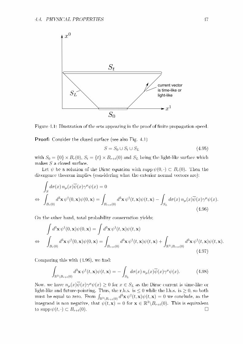
4.4. PHYSICAL PROPERTIES 47
current vectoris time-like orlight-like
Figure 4.1: Illustration of the sets appearing in the proof of nite propagation speed.
Proof: Consider the closed surface (see also Fig. 4.1)
S = S0 ∪ St ∪ SL (4.95)
with S0 = 0×Br(0), St = t×Br+t(0) and SL being the light-like surface whichmakes S a closed surface.
Let ψ be a solution of the Dirac equation with suppψ(0, ·) ⊂ Br(0). Then thedivergence theorem implies (considering what the exterior normal vectors are):∫
S
dσ(x)nµ(x)ψ(x)γµψ(x) = 0
⇔∫Br(0)
d3xψ†(0,x)ψ(0,x) =
∫Br+t(0)
d3xψ†(t,x)ψ(t,x)−∫SL
dσ(x)nµ(x)ψ(x)γµψ(x).
(4.96)
On the other hand, total probability conservation yields:∫d3xψ†(0,x)ψ(0,x) =
∫d3xψ†(t,x)ψ(t,x)
⇔∫Br(0)
d3xψ†(0,x)ψ(0,x) =
∫Br+t(0)
d3xψ†(t,x)ψ(t,x) +
∫R3\Br+t(0)
d3xψ†(t,x)ψ(t,x).
(4.97)
Comparing this with (4.96), we nd:∫R3\Br+t(0)
d3xψ†(t,x)ψ(t,x) = −∫SL
dσ(x)nµ(x)ψ(x)γµψ(x). (4.98)
Now, we have nµ(x)ψ(x)γµψ(x) ≥ 0 for x ∈ SL as the Dirac current is time-like orlight-like and future-pointing. Thus, the r.h.s. is ≤ 0 while the l.h.s. is ≥ 0, so bothmust be equal to zero. From
∫R3\Br+t(0)
d3xψ†(t,x)ψ(t,x) = 0 we conclude, as the
integrand is non-negative, that ψ(t,x) = 0 for x ∈ R3\Br+t(0). This is equivalentto suppψ(t, ·) ⊂ Br+t(0).
48 CHAPTER 4. THE DIRAC EQUATION
Plane wave solutions. Similarly as for the KG equation, we are looking forsolutions of the form
ψ(x) = u(p) e−ipµxµ
. (4.99)
Here, u : R4 → C4 is a vector-valued function. Plugging in the ansatz (4.99), weobtain the equation
(γµpµ −m)u(p) = 0. (4.100)
This is just a matrix-vector equation with a parameter p. By acting on (4.100)with (γνpν + m), one can see that each component of u satises the KG equation.Therefore, we must have
p2 −m2 = 0 ⇔ p0 = ±√
p2 +m2. (4.101)
We consider the case p0 = +√
p2 +m2 = ω(p) rst and call the respective functionsu(p) =: u+(p). Then (4.100) becomes:
(α · p + βm)u+(p) = ω(p)u+(p). (4.102)
In our representation of the α, β-matrices this is equivalent to the following twoequations for (u1, u2) = u+:
σ · pu2 +mu1 = ω(p)u1, (4.103)
σ · pu1 −mu2 = ω(p)u2. (4.104)
As ω(p) > 0 > −m, this can be easily solved for u2:
u2(p) =σ · p
ω(p) +mu1(p). (4.105)
Inserting this back into (4.103), we obtain:((σ · p)2
ω(p) +m+m
)u1 = ω(p)u1. (4.106)
Now, we have (σ · p)2 = p2 and
p2
ω(p) +m=ω(p)2 −m2
ω(p) +m= ω(p)−m. (4.107)
Therefore, (4.103) holds identically. We thus have found a class of solutions of theDirac equation, one for each p and each u1. As u1 has two components, there aretwo linearly independent solutions u
(i)+ , i = 1, 2 for each p:
u(i)+ (p) =
√ω(p) +m
2ω(p)
(χi
σ·pω(p)+m
χi
), i = 1, 2. (4.108)
Here, χ1 = (1, 0) and χ2 = (0, 1), and prefactor of the vector is a normalization
constant such that (u(i)+ (p))†u
(i)+ (p) = 1.
4.4. PHYSICAL PROPERTIES 49
Now we turn to the case p0 = −ω(p). As the KG equation, the Dirac equationalso admits negative energies. We call the respective solutions u−(p). Proceed-ing similarly as above, we obtain the following two linearly independent solutionsfor each p:
u(i)− (p) =
√ω(p) +m
2ω(p)
(− σ·pω(p)+m
χiχi
), i = 1, 2, (4.109)
where again χ1 = (1, 0)T and χ2 = (0, 1)T .Accordingly, a large class of solutions of the Dirac equation can be obtained by
superposing these plane-wave solutions. For φ+, φ− ∈ L1(R3) ∩ L2(R3)
ψ(t,x) =∑j=1,2
∫d3p
(2π)3
(φ+(p)u
(j)+ (p)eip·x−iω(p)t + φ−(p)u
(j)− (p)eip·x+iω(p)t
)(4.110)
yields a solution of the Dirac equation.
Discussion of negative energies, Dirac sea. For the KG equation, negativeenergy solutions were problematic mainly because then the 0-component of the KGcurrent could become negative. For the Dirac equation, we have
j0 = ψ†ψ ≥ 0 (4.111)
independently of whether ψ is a negative energy solution or not. The probabilityinterpretation is therefore not aected by negative energies. Thus, at least the basiclogical framework of how we would like to use the Dirac equation is consistent.
However, one might worry that negative energies could cause a dierent problem.Namely, if the Dirac equation gets coupled to other matter or elds, could one notgenerate innite amounts of energy if the Dirac particle lowers its energy innitelyand emits it in form of radiation? Whether or not this really happens, has (tothe best of my knowledge) never been analyzed comprehensively. The answer mayalso depend on the type of interaction between light and matter. Usually, it isdescribed by quantum electrodynamics. We shall not treat this theory here. Thegeneral feeling, however, is that the aforementioned innite lowering of energiescould indeed happen, and has to be prevented by some mechanism as one does notobserve it in nature.
To prevent the problem, Dirac postulated that for a multi-electron system, therewould be innitely many electrons occupying3 the negative energy states. Thisinnity of negative energy electrons has been called Dirac sea. If all the negativeenergy states were occupied, additional electrons with positive energies could notlower their energy below their rest energy mc2 due to the Pauli principle. The greatmajority of the Dirac sea could then not interact with positive energy electrons(only those just below E = −m2) and would thus not be seen in experiments. Diracfurthermore showed that if one of the negative energy states is unoccupied, it can bedescribed by the charge conjugated Dirac equation. Dirac rst thought this chargeconjugated equation would describe the proton. However, it quickly turned out
3"Occupying" is meant in the sense of second quantization and the occupation number repre-sentation of states in Fock space.
50 CHAPTER 4. THE DIRAC EQUATION
that this could not be the case (due to the mass) and that it instead describes ananti-electron, the positron. Historically, anti-particles were found experimentallyshortly after Dirac's discoveries. Besides showing that spin is logically necessaryfor relativistic wave functions, the prediction of anti-particles is one of the greatestsuccesses of the Dirac equation.
In the prevailing interpretation of quantum electrodynamics, one re-denes theDirac sea as the vacuum state and treats the absence of a particle in the Dirac sea asits own type of particle, the positron. The transition of a negative energy electronin the Dirac sea to positive energies (leaving back a hole in the Dirac sea) then getsre-interpreted as the creation of an electron-anti-electron pair (both with positiveenergies). The two views can be translated into each other and are (more or less)mathematically (though not conceptually) equivalent.
4.5 Solution theory
4.5.1 Classical solutions
In this section, we are looking for solutions ψ ∈ C1(R4,C4) of the initial valueproblem
ψ(0,x) = ψ0(x), x ∈ R3,(iγµ∂µ −m)ψ(t, x) = 0, t 6= 0,x ∈ R3,
(4.112)
where ψ0 ∈ C1(R3,C4) ∩ L2(R3,C4) is a given function.First, we prove the uniqueness of the solution.
Theorem 4.5.1 Let ψ1, ψ2 ∈ C1(R4,C4) be a solution of (4.112) such that theirrestrictions ψi|Σ , i = 1, 2 lie in L2(Σ,C4) for every space-like hyperplane Σ ⊂ M.Then we have ψ1 = ψ2.
Proof: You have already shown this on Sheet 6, Exercise 3 using the technique of"energy" integrals applied to the total probability integral P (Σ) =
∫Σdσ(x)nµ(x)ψ(x)γµψ(x).
Next, we show that provided there exists a solution of (4.112), it can be foundvia reduction to a KG equation with special initial data.
Theorem 4.5.2 Let ψ0 ∈ C3(R3,C4) and assume the IVP (4.112) has a solutionψ ∈ C2(R4,C4) such that for every space-like hyperplane Σ ⊂ M, the restrictionψ|Σ lies in L2(Σ,C4). Then the solution is unique and its spin components ψj, j =1, 2, 3, 4 are given by
ψj(τ,y) =τ
4π
∫∂Bτ (0)
dΩx gj(x + y)− m
4π
∫Bτ (0)
d3xJ1(m
√τ 2 − |x|2)√
τ 2 − |x|2gj(x + y)
+∂
∂τ
(τ
4π
∫∂Bτ (0)
dΩx fj(x + y)− m
4π
∫Bτ (0)
d3xJ1(m
√τ 2 − |x|2)√
τ 2 − |x|2fj(x + y)
),
(4.113)
where for j = 1, 2, 3, 4fj(x) = (ψ0)j(x), x ∈ R3 (4.114)
4.5. SOLUTION THEORY 51
andgj(x) = −i(αk∂kψ0)j(x) +m(βψ0)j(x), x ∈ R3. (4.115)
Proof: We already know that under the given conditions, the solution ψ is unique.Furthermore, as ψ ∈ C2(R4,C4), each component ψj solves the KG equation. Theinitial data are given by (4.114) and by (4.115). The latter can be seen by dierenti-ating ψ w.r.t. t and using the fact that ψ is a solution of the Dirac equation. By the-orems 3.3.1 and 3.3.2, we obtain that the unique solution of the initial value problemof the KG equation for the j-th component is given by (4.113), j = 1, 2, 3, 4. Here,the regularity property ψ0 ∈ C3(R3,C4) is required. Now, as the IVP of the Diracequation has by assumption one solution (and by uniqueness exactly one) which alsosatises the IVP of the KG equation, this solution coincides with (4.113).
Remark. With some eort, one can also demonstrate directly that the formula(4.113) yields a solution (i.e., without relying on the a-priori assumption that aC2-solution of the Dirac equation exists).
4.5.2 Hilbert space valued solutions
In this section we study a more abstract notion of solution of the Dirac equationwhich is common in mathematical physics and functional analysis.
Hamiltonian formulation of the Dirac equation. By multiplying the Diracequation with γ0, one can rewrite it as follows:
i∂tψ(t,x) = HDiracψ(t,x) (4.116)
with the Dirac Hamiltonian
HDirac = −iαj∂j +mβ (sum over j = 1, 2, 3). (4.117)
One now interprets (4.116) as an equation on Hilbert space,
H = L2(R3,C4) (4.118)
with scalar product
〈ψ, φ〉 =
∫d3xψ†(x)ϕ(x). (4.119)
Note that the functions ψ ∈ H are time-independent. (The Hilbert space formu-lation is therefore not manifestly Lorentz invariant.) One thus interprets the wavefunction ψ(t,x) in the Dirac equation as a map
ψ : R→H , t 7→ ψ(t). (4.120)
The Dirac equation is then to be understood as an ordinary dierential equation forthe Hilbert space valued map ψ(t) as follows:
idψ(t)
dt= HDiracψ(t). (4.121)
52 CHAPTER 4. THE DIRAC EQUATION
HDirac is, as usual for dierential operators, an unbounded operator on H . It canthus not be dened on the whole of H but only on a certain domain, D(HDirac) ⊂H . It turns out that for the Dirac operator, a suitable domain is given by
D(HDirac) = H1(R3)4, (4.122)
the rst Sobolev space of functions from R3 to C4. (This means, one can take therst weak derivatives of ψ in the spatial directions.)
The goal now is to show that HDirac is self-adjoint on D(HDirac). Then, byStone's theorem,
U(t) = exp(−iHDiract) (4.123)
denes a strongly continuous unitary one-parameter group on H . Furthermore, wehave:
idU(t)
dt
∣∣∣∣t=0
= HDirac. (4.124)
Thus, (4.121) with initial condition ψ(0) = ψ0 ∈H has the unique solution
ψ(t) = U(t)ψ0. (4.125)
Indeed, we have the following theorem (Thaller p. 11):
Theorem 4.5.3 HDirac is self-adjoint on the rst Sobolev space
D(HDirac) = H1(R3)4. (4.126)
Its spectrum is purely continuous4 and given by
σ(HDirac) = (−∞,−m] ∪ [m,∞). (4.127)
Proof: We rst prove the statement about self-adjointness and spectrum. The ideais to reduce the problem to a multiplication operator with a self-adjoint matrixvia Fourier transformation (similarly as for the plane-wave solutions of the Diracequation). Let F denote the Fourier transformation. F is rst dened on integrable(L1) functions but can be uniquely extended to a unitary operator on H = L2(R3)4.For the Dirac operator, we have:
(FHDiracF)(p) = h(p) :=
(m12 σ · pσ · p −m12
). (4.128)
For each p, this is a Hermitian 4× 4 matrix with eigenvalues
λ1(|p|) = λ2(|p|) = −λ3(|p|) = −λ4(|p|) =√
p2 +m2 = ω(p). (4.129)
As h(p) is Hermitian, there is a unitary transformation u(p) which diagonalizesh(p). Explicitly:
u(p) =(m+ ω(p))14 + βα · p√
2ω(p)(m+ ω(p)). (4.130)
4The continuous spectrum of an operator A on H is dened as those λ ∈ C which make therange of A− λ1 a proper dense subset of H .
4.5. SOLUTION THEORY 53
Then:
u(p)h(p)u(p)−1 = β ω(p). (4.131)
Overall, we see that unitary the operator
W = uF (4.132)
converts HDirac into a multiplication operator with a diagonal matrix
(WHDiracW−1)(p) = β ω(p) (4.133)
on the Hilbert space L2(R3, d3p).Because of this unitary equivalence to this self-adjoint multiplication operator,HDirac
itself is self-adjoint on
D(HDirac) =W−1D(β ω(·)) = F−1u−1D(ω(·)) = F−1D(ω(·)). (4.134)
The last step follows as u−1 is a multiplication operator with a unitary matrix whichdoes not change the domain of a multiplication operator.Now the rst Sobolev space H1(R3)4 is by denition given by the inverse Fouriertransformation of the set
f ∈ L2(R3, d3p)4 : (1 + |p|2)1/2f ∈ L2(R3, d3p)4. (4.135)
As ω(p) =√m2 + |p|2, this set equals D(ω(·)) (for m 6= 0).
Similarly, the spectrum of HDirac is given by the spectrum of the multiplicationoperator βω(·) which is given by (−∞,−m] ∪ [m,∞).
Representation of the solution by an integral formula.
Theorem 4.5.4 (Thaller p. 15) Let ψ0 ∈ S(R3)4 (the set of rapidly decreasingSchwarz functions with four components). Then for t 6= 0, the unique solution ψ ofthe Dirac equation with initial data ψ(0, ·) = ψ0(·) is given by:
ψ(t,x) = −i∫R3
d3y S(t,x− y)γ0ψ0(y), (4.136)
where S(t,x) is the distribution given by
S(t,x) = (iγµ∂µ +m)∆(x) (4.137)
and
∆(x) =sgn(x0)
2π
[δ(xµx
µ)− m
2θ(xµx
µ)J1(m
√xµxµ)
√xµxµ
]. (4.138)
For the proof, see Thaller pp. 16-18 (note the dierent sign conventions).
54 CHAPTER 4. THE DIRAC EQUATION
Remarks.
1. The representation formula for the solution (4.136) can be shown to be iden-tical to our previous result (4.113), at least for t > 0.
2. The formula (4.136) is the analog of the solution formula (3.44) for the KGequation via its retarded Green's function.
3. S(t,x) is the called the propagator of the Dirac equation. For t > 0, S(t,x)coincides with the retarded Green's function Sret(t,x) of the Dirac equation,and for t < 0 with minus the advanced Green's function −Sadv(t,x).
4. One obtains Green's functions of the Dirac equation from those of the KGequation by applying the operator −(iγµ∂µ +m):
S(i)(x) = −(iγµ∂µ +m)G(i)(x) (4.139)
where G(i)(x) is a Green's function of the KG equation.
5. ∆(x) = Gret(x)−Gadv(x), where Gret, Gadv are retarded and advanced Green'sfunctions of the KG equation, respectively. So for x0 > 0, ∆(x) = Gret(x)which agrees exactly with the distribution K we used for the solution of initialvalue problem for the KG equation and t > 0.
Generalization of the representation formula to arbitrary space-like hy-perplanes. For every space-like hyperplane Σ ⊂M with future-pointing unit nor-mal vector eld n and every ψΣ ∈ S(Σ)4, the unique solution of the initial valueproblem
ψ(x) = ψΣ(x), x ∈ Σ (4.140)
of the Dirac equation is given by:
ψ(x) = −i∫
Σ
dσ(y)S(x− y)γµnµ(y)ψΣ(y). (4.141)
By using this formula (i) for x ∈ Σ or (ii) repeatedly for two dierent hyperplanesΣ,Σ′, we obtain the following distributional identities (Sheet 10, Exercise 3):
(i) S(0,x) = iγ0δ(3)(x),
(ii) −i∫
Σdσ(y)S(x−y)γµnµ(y)S(y−z) = S(x−z) for every space-like hyperplane
Σ.
Remark: The formula (4.141) also holds for more general curved space-like hy-persurfaces Σ.
4.5. SOLUTION THEORY 55
Natural Hilbert spaces for the Dirac equation. If we want to have a space-time picture for the Dirac equation, the Hilbert space H = L2(R3,C4) is not partic-ularly natural. The fact that probability conservation holds on arbitrary space-likehyperplanes (in fact, on arbitrary space-like Cauchy surfaces) Σ ⊂ M, suggests todene the following Hilbert spaces:
HΣ = L2(Σ,C4, dσ(x)) (4.142)
with scalar product (→ Sheet 10, Exercise 2):
〈ψ, ϕ〉Σ =
∫Σ
dσ(x)nµ(x)ψ(x)γµϕ(x). (4.143)
This denes a norm in the usual way,
‖ψ‖Σ =√〈ψ, ψ〉Σ. (4.144)
Then, evaluating the solution formula (4.141) for x on a space-like hyperplane Σ′
denes an injective mapUΣ′
Σ : S(Σ)4 →HΣ′ . (4.145)
Total probability conservation means that
‖ψ|Σ‖Σ = ‖ψ|Σ′‖Σ′ = ‖UΣ′
Σ ψ|Σ‖Σ′ . (4.146)
Together with the uniqueness of the solution this suggests that U can be extendedto a unitary map between the full Hilbert spaces HΣ and HΣ′ , i.e.
UΣ′
Σ : HΣ →HΣ′ . (4.147)
The previous unitary operator U(t) = exp(−iHDiract) can be thought of as thespecial case of UΣ′
Σ for Σ = Σt=0 and Σ′ = Σt. One should note that the Hilbertspaces HΣt can, for every t ∈ R, be canonically identied with H = L2(R3,C4),namely through
HΣt 3 ψ|Σt ≡ ψ(t, ·) ∈H . (4.148)
56 CHAPTER 4. THE DIRAC EQUATION
5. The multi-time formalism
In this chapter, we are concerned with the description of many relativistic quantumparticles.
5.1 Motivation
The usual way to a many-body quantum theory in the Schrödinger pic-ture. The usual way from a single-particle to a many-particle quantum theory isto take tensor products of the single-particle Hilbert spaces and to take the sum ofthe Hamiltonians as the overall free (non-interacting) Hamiltonian.
We consider the case of N particles, each described by a Dirac equation (withpossibly dierent masses). The (time-independent) Hilbert space then is H =L2(R3,C4), and its N -fold tensor product yields:
H ⊗N ∼= L2(R3N ,C4N ). (5.1)
The idea is that the wave function, ϕ, then satises the Schrödinger equation
idϕ(t)
dt=
N∑k=1
HDirack ϕ(t) + V ϕ(t) (5.2)
where
HDirack =
3∑j=1
(−iγ0kγ
jk∂k,j) + γ0
kmk (5.3)
with ∂k,µ = ∂∂xµk
and
γµk = 1× · · · ⊗ 1 ⊗γµ⊗︸ ︷︷ ︸k-th place
1⊗ · · · ⊗ 1. (5.4)
Moreover, V is a multiplication operator with a function V (t,x1, ...,xN) with valuesin the symmetric matrices.
Overall, that means ϕ has to be viewed as a map
ϕ : R× R3N → (C4)⊗N ∼= C4N , (t,x1, ...,xN) 7→ ϕ(t,x1, ...,xN). (5.5)
We call this map the single-time wave function.When formulated as a PDE (instead of as an ODE on Hilbert space), the
Schrödinger equation becomes:
i∂tϕ =N∑k=1
(−iγ0
kγjk∂k,j + γ0
kmk
)ϕ+ V (t,x1, ...,xN)ϕ. (5.6)
57
58 CHAPTER 5. THE MULTI-TIME FORMALISM
Limitation of the usual approach. Our goal is to obtain a relativistic theory.However, the above approach suers from the following problems (for N ≥ 2):
1. It is not clear how to Lorentz-transform the single-time wave function. Thisis because the argument (t,x1, ...,xN) contains N spatial variables but onlyone time. For such variables, there is no pre-dened transformation behaviorunder Lorentz boosts. (For rotation, on the other hand, we could rotate eachxi in the same way.)
2. Relatedly, the single-time Schrödinger equation (5.6) is not manifestly Lorentzinvariant.
3. The Born rule corresponding to the outlined theory is:
(ϕ†ϕ)(t,x1, ...,xN) d3x1 · · · d3xN is the probability to nd N parti-cles, each particle i at a location in the innitesimal volume d3xiaround xi ∈ R3 at time t.
As this statement refers to a particular time coordinate t, it only holds forone particular Lorentz frame. We would like to have a frame-independentstatement instead.
Derivation of multi-time wave functions from Lorentz transformations ofcongurations. We now give an argument in favor of a relativistic type of wavefunction which overcomes the above-mentioned problems.
From the Born rule, we can see that the argument of ϕ, (t,x1, ...,xN) refers toa spatial conguration (x1, ...,xN) ∈ R3 at a certain time t. The same space-timeconguration is expressed by the following collection of 4-vectors:
((t,x1), ..., (t,xN)). (5.7)
Given this collection of 4-vectors, it is now clear how a Lorentz transformation Λacts, namely by applying Λ to each 4-vector:
((t,x1), ..., (t,xN))Λ→ (Λ(t,x1), ...,Λ(t,xN)) = ((t′1,x
′1), ..., (t′N ,x
′N)). (5.8)
The important point is that in general, t′j 6= t′k for j 6= k. So we end up with Ndierent time variables after the Lorentz transformation.
We now want to apply this insight to the argument of the wave function. To thisend, we must rst identify ϕ(t,x1, ...,xN) as the equal-time case of a more generalobject ψ(t1,xN , ..., tN ,xN) which may exist for tj 6= tk, i.e.:
ϕ(t,x1, ...,xN) = ψ(t,x1, ..., t,xN). (5.9)
Recalling the transformation behavior of the wave function of the Dirac equation(4.41), we expect the following transformation behavior:
ψ′(x′1, ..., x′N) = S[Λ]⊗Nψ(x1, ..., xN). (5.10)

5.2. EVOLUTION EQUATIONS 59
This implies:
ψ′(t,x1, ..., t,xN) = S[Λ]⊗Nψ(Λ−1(t,x1), ....,Λ−1(t,xN)) = S[Λ]⊗Nψ(t′1,x′1, ..., t
′N ,x
′N),
(5.11)where in general t′j 6= t′k for j 6= k (here x′i = Λ−1xi). So we nd that ψ is indeedneeded on space-time congurations with dierent times.
Denition: Let N ∈ N, N ≥ 2 be the number of particles and K ∈ N the numberof spin components per particle. Moreover, let Ω be a Poincaré invariant1 subset ofR4N . Then a multi-time wave function is a map
ψ : Ω ⊂ R4N → CKN
, (x1, ..., xN) 7→ ψ(x1, ..., xN). (5.12)
Remark. Natural choices for Ω are Ω = R4N and Ω = S , the set of space-likecongurations:
S = (x1, ..., xN) ∈ R4N : ∀j 6= k : (xj − xk)µ(xj − xk)µ < 0. (5.13)
You will show on Sheet 11, Exercise 2 that for N = 2, S is the smallestPoincaré invariant set which contains the equal-time collision-free congurationsC = (x1, ..., xN) ∈ R4N : xi = xj ∀i, j and xj 6= xk ∀j 6= k.
Historical Remark. The idea of multi-time wave functions dates back to Dirac'spaper
P. A. M. Dirac, Relativistic Quantum Mechanics, Proc. R. Soc. Lond. A,136:453464, 1932.
A recent overview of the theory of multi-time wave functions can be found in:
M. Lienert, S. Petrat, and R. Tumulka. Multi-time wave functions. J. Phys.Conf. Ser., 880(1):012006, 2017. https://doi.org/10.1088/1742-6596/
880/1/012006
5.2 Evolution equations
Multi-time Schrödinger equations. A multi-time wave function has N timecoordinates. Therefore, it was Dirac's idea that one needs one evolution equationfor each time coordinate. This leads to a system of N equations which ψ needs tosatisfy simultaneously:
i∂t1ψ = H1ψ,
... (5.14)
i∂tNψ = HNψ.
1A Poincaré transformation (a,Λ) acts on (x1, ..., xN ) ∈ R4N as (Λx1 + a, ...,ΛxN + a).
60 CHAPTER 5. THE MULTI-TIME FORMALISM
Here, ti = x0i . It is understood that one should be able to rewrite (5.14) in a
manifestly Lorentz invariant form, such as in the example of free multi-time Diracequations:
(iγµk∂k,µ −mk)ψ(x1, ..., xN) = 0, k = 1, ..., N. (5.15)
You will analyze these equations in more detail on Sheet 11, Exercise 1.The operators Hk in (5.14) are supposed to be dierential operators on an ap-
propriate function space. There are dierent ways to interpret the system (5.14)mathematically. Perhaps the most appropriate and straightforward way is as a sys-tem of N partial dierential equations. Alternatively, one can also view it as asystem of N equations for a Hilbert space valued function of N time variables,
ψ : RN →H , (t1, ..., tN) 7→ ψ(t1, ..., tN) ∈H . (5.16)
Note that in this view, the choice H = L2(R3N ,C4N ) distinguishes a particularLorentz frame which is, from a relativistic standpoint, not very natural. However,one can still use it as a mathematical convenience (bearing in mind that the involvedframe is somewhat arbitrary).
We re-obtain the familiar single-time Schrödinger equation from the multi-timeequations (5.14) by considering i∂tϕ(t) = i∂tψ(t, · · · , t) and using the chain rule:
i∂tψ(t, · · · , t) =N∑k=1
Hkψ(t, ..., t). (5.17)
That means, the operators Hk sum up to the Hamiltonian of the system. They aretherefore called partial Hamiltonians.
Initial data. The role of the multi-time equations (5.14) is to determine ψ uniquelygiven initial data on a set of the form ΣN where Σ ⊂M is a Cauchy surface. Perhapsmost conveniently, one can choose Σ = Σt=0 in a particular Lorentz frame. Theninitial data are given by
ψ(0,x1, ..., 0,xN) = ψ0(x1, ...,xN), xi ∈ R3, i = 1, ..., N (5.18)
for some given function ψ0 : R3N → CKN.
Now the crucial question is: when is it possible to uniquely solve (5.14) forall initial data (5.18)? This is an important question, as (5.14) is a system of Nsimultaneous PDEs which might not always have a solution. We shall now work outconditions when this is possible. We start with the Hilbert space view, and the casethat the partial Hamiltonians Hk can be viewed as time-independent operators onHilbert space.
Consistency conditions.
Denition: Let H be a Hilbert space. A strongly continuous unitary N-parametergroup is a map U from RN into the set of unitary operators on H such that U(0) =1 and for t, s ∈ RN : U(t)U(s) = U(t + s). Furthermore, strongly continuousmeans that each one-parameter subgroup Uj(tj) = U(0, ..., 0, tj, 0, ..., 0) is stronglycontinuous. According to the theorem of Stone this means that i d
dtjUj(tj)|tj=0 exists
and is given by a self-adjoint operator.
5.2. EVOLUTION EQUATIONS 61
Denition: We say that the multi-time equations (5.14) have a Hilbert-space valuedsolution for all initial data ψ0 ∈H if and only if there exists a strongly continuousunitary N -parameter group U(t1, ..., tN) with
i∂
∂tjU(0, ..., 0, tj, 0, ..., 0) = Hj U(0, ..., 0, tj, 0, ..., 0). (5.19)
(Then the solution is given by ψ(t1, ..., tN) = U(t1, ..., tN)ψ0.)
Theorem 5.2.1 Let H be a Hilbert space and H1, ..., HN be time-independent self-adjoint operators on H . Then there exists a Hilbert-space valued solution of theinitial value problem
ψ(0, ..., 0) = ψ0 ∈H ,i∂tkψ(t1, ..., tN) = Hkψ(t1, ..., tN), k = 1, ..., Nψ, t1, ..., tN ∈ R (5.20)
for all initial data ψ0 ∈H if and only if
[Hj, Hk] = 0 ∀j 6= k (5.21)
(in the spectral sense)2.
Proof: "⇒" For j, k = 1, ..., N, j 6= k, let Hj be self-adjoint and let [Hj, Hk] = 0in the spectral sense (all spectral projections from the spectral theorem of theseself-adjoint operators commute). The self-adjointness of each Hj allows us to denethe strongly continuous unitary one-parameter groups
Uj(tj) = e−iHjtj . (5.22)
Because of (5.21), these groups commute with each other for j 6= k. That meansthat
U(t1, ..., tN) = e−iH1t1 · · · e−iHN tN (5.23)
denes a strongly continuous unitary N -parameter group. (Note that the dierentexponentials have to commute to ensure this.) Moreover,
i∂
∂tkU(t1, ..., tN) = HkU(t1, ..., tN). (5.24)
Therefore,
ψ(t1, ..., tN) = U(t1, ..., tN)ψ0 (5.25)
is a solution of the IVP (5.20).
"⇐" Let (5.20) have an H -valued solution for all initial data. By the denition ofthe Hilbert space valued solution, there then exists a strongly continuous unitaryN -parameter group U(t1, ..., tN) whose one-parameter subgroups Uj(tj) are given by
2This means that all spectral projections of the operators have to commute. See the spectraltheorem.
62 CHAPTER 5. THE MULTI-TIME FORMALISM
e−iHjtj according to Stone's theorem. Then, as U(t+s) = U(t)U(s) for all t, s ∈ RN ,we have, for all j 6= k:
U(..., tj, ..., tk, ...) = Uj(tj)U(..., tj = 0, ..., tk, ...) = Uj(tj)Uk(tk)U(..., tj = 0, ..., tk = 0, ...)
= e−iHjtje−iHktkU(..., tj = 0, ..., tk = 0, ...) (5.26)
On the other hand, we obtain analogously:
U(..., tj, ..., tk, ...) = e−iHktke−iHjtjU(..., tj = 0, ..., tk = 0, ...). (5.27)
Setting all other tl = 0, this implies e−iHjtje−iHktk = e−iHktke−iHjtj which is equiva-lent to [Hj, Hk] = 0 in the spectral sense.
Remark. [Hj, Hk] ∀j 6= k is called the consistency condition for the multi-timeequations (5.14). In the case that the partial Hamiltonians are time-dependentmaps Hj = H(t1, ..., tN) from RN into the self-adjoint operators, the condition getsreplaced by3
[Hj, Hk]− i∂Hk
∂tj+ i
∂Hj
∂tk= 0 ∀j 6= k. (5.28)
No-go theorem for potentials. The consistency conditions (5.28) are fairly re-strictive. We shall now see that they rule out interaction potentials (even Poincaréinvariant ones).
Theorem 5.2.2 For k = 1, ..., N let
Hk(t1, ..., tN) = HDirack + Vk(x1, ..., xN) (5.29)
where for each k, Vk : R4N → R is a smooth function. Then:
(i) The consistency conditions (5.28) are satised only if Vk does not depend onxj for j 6= k, k, j = 1, ..., N .
(ii) If in addition all Vk are Poincaré invariant, then (5.28) is only satised ifVk = const for all k = 1, ..., N .
Proof: (i) We write out the consistency conditions (5.28) in detail in our case.Using that [Vj, Vk] = 0 and [HDirac
j , HDirack ] = 0, we nd:
0 = [Hj, Hk]− i∂Vk∂tj
+ i∂Vj∂tk
= [HDiracj , Vk]− [HDirac
k , Vj] + i
(∂Vj∂tk− ∂Vk∂tj
)= −i
3∑l=1
(γ0j γ
lj
∂Vk∂xlj− γ0
kγlk
∂Vj∂xlk
)+ i
(∂Vj∂tk− ∂Vk∂tj
). (5.30)
3See S. Petrat and R. Tumulka. J. Math. Phys., 55(032302), 2014.
5.3. PROBABILITY CONSERVATION AND GENERALIZED BORN RULE 63
Now, the matrices 1, γ0j γ
lj, γ
0kγ
lk, j 6= k, l = 1, 2, 3 are all linearly independent. Thus
their coecients have to vanish separately and we obtain:
∂Vj∂tk
=∂Vk∂tj
(5.31)
and∂Vk∂xlj
= 0, (5.32)
j 6= k = 1, ..., N, l = 1, 2, 3. (5.32) already shows claim (i).
(ii) Lorentz invariance now implies that Vk must not depend on x0j , either, j 6= k,
j, k = 1, ..., N . That means, Vk(x1, ..., xN) = Vk(xk) for some smooth function Vk :R4 → C, k = 1, ..., N . Then it follows from translation invariance that Vk = const,k = 1, ..., N .
Remarks.
1. The rst rigorous result in the spirit of the above theorem was obtained byPetrat and Tumulka4. They do not assume Poincaré invariance of the po-tentials and prove that even for potentials which are not Poincaré invariantthe multi-time equations must be gauge equivalent to equations with purelyexternal potentials (no interaction).
2. The above theorem only treats the case of scalar potentials, such as Coulombpotentials Vj = 1
2
∑k 6=j
1|xj−xk|
(or a Poincaré invariant version of this). There
are also more elaborate versions of the theorem for matrix valued potentials.Perhaps the most complete result is a theorem by Nickel and Deckert.5 Theyadmit arbitrary matrix-valued potentials Vj : R4N → (C4)⊗N and prove thatthere are no Poincaré invariant ones besides Vj = 0∀j which satisfy the con-sistency conditions.
3. A similar result also holds for −∆k, the k-th Laplacian, instead of HDirack . (→
Sheet 12, Exercise 1). This shows that it is really the form of the multi-timesystem (5.14) which excludes interaction potentials. Poincaré invariance doesnot play an important role in this.
Conclusion. Potentials are not a viable mechanism for interaction in multi-timeequations, and an alternative mechanism is necessary. One such possibility will bepresented in Sec. 5.4.
5.3 Probability conservation and generalized Born
rule
In this section, we discuss the question how to generalize the Born rule to arbitraryspace-like surfaces using a multi-time wave function. Physically, this means we now
4See S. Petrat and R. Tumulka. J. Math. Phys., 55(032302), 2014.5L. Nickel and D.-A. Deckert. J. Math. Phys. 57 072301 (2016).
64 CHAPTER 5. THE MULTI-TIME FORMALISM
describe the detection probabilities of particles at dierent times (but such that thedetection events remain space-like to each other). The discussion proceeds at thecase of a xed number N of particles.
Tensor currents. Similarly to the Dirac equation, where we had a conservedcurrent density vector eld jµ(x), we are now looking for conserved tensor currents.
Denition: For N particles and Minkowski spacetime, a tensor current is a collec-tion of continuously dierentiable maps (µ1, ..., µN = 0, 1, 2, 3)
jµ1...µN : Ω ⊂MN → R, (x1, ..., xN)→ jµ1...µN (x1, ..., xN). (5.33)
It is called conserved if for all k = 1, ..., N :
∂xµkkjµ1...µk...µN = 0, µ1, ..., µk, ...µN = 0, 1, 2, 3, (5.34)
where (·) denotes omission.
Example. Let ψ be a C1 solution of the free multi-time Dirac equations (iγµk∂k,µ−mk)ψ = 0, k = 1, ..., N . Then
jµ1...µN (x1, ..., xN) = ψ(x1, ..., xN)γµ1
1 · · · γµNN ψ(x1, ..., xN) (5.35)
denes a conserved tensor current on MN (see Sheet 11, Exercise 1).For independent particles, the wave function is a tensor product of N single-
particle wave functions ψk : M→ C4 which all solve the Dirac equation, i.e.:
ψ(x1, ..., xN) = ψ1(x1)⊗ · · · ⊗ ψN(xN). (5.36)
For such a wave function, the Dirac tensor current (5.35) becomes:
jµ1...µN (x1, ..., xN) = jµ1
1 (x1) · · · jµNN (xN), (5.37)
where jµkk (xk) = ψk(xk)γµψk(xk). That means, it becomes the product of N single-
particle Dirac currents.As a consequence of the behavior of ψ under Lorentz transformations Λ (see Eq.
(5.10)), the Dirac tensor current transforms as
j′µ1...µN (x′1, ..., x
′N) = Λµ1
ν1 · · ·ΛµNνN j
ν1...νN (x1, ..., xN). (5.38)
Given appropriate properties, the idea is to dene a probability density via thetensor current. An important property such that this works is the following.
Denition: A tensor current j is called positive denite if for all x1, ..., xN ∈ Mand all future-pointing time-like vectors n1, ..., nN ∈M:
jµ1...µN (x1, ..., xN)nµ1 · · ·nµN ≥ 0 (5.39)
and equality implies j(x1, ..., xN) = 0.
Denition: Let j be a positive denite and conserved tensor current and Σ bea space-like hyperplane (or more generally a smooth Cauchy surface) with future-pointing unit normal vector eld n. Then we call the non-negative function denedby
ρΣ(x1, ..., xN) = jµ1...µN (x1, ..., xN)nµ1(x1) · · ·nµN (xN) (5.40)
the density of j with respect to Σ.
5.3. PROBABILITY CONSERVATION AND GENERALIZED BORN RULE 65
Remark. This denition generalizes the usual notion of a probability density in anatural way. For example, for the Dirac tensor current (5.35) we have:
(i) For N = 1, ρΣ(x) = jµ(x)nµ(x) reduces to the familiar probability densitywith respect to Σ.
(ii) For N ≥ 2 and an equal-time hyperplane Σt in a certain frame, we have n(x) =(1, 0, 0, 0) and thus ρΣt(t,x1, ..., t,xN) = (ψ†ψ)(t,x1, ..., t,xN) = (ϕ†ϕ)(t,x1, ...,xN).So the density ρΣ reduces to the usual single-time probability density in thatcase (as expected).
In general, one can integrate ρΣ over arbitrary subsets of a space-like hyperplane(smooth Cauchy surface). Together with the above, this suggests:
Generalized Born rule. Let Σ ⊂M be a space-like hyperplane (smooth Cauchysurface) and ρΣ the associated density. Furthermore, assume that ρΣ is normalizedin the sense ∫
Σ
dσ(x1) · · ·∫
Σ
dσ(xN) ρΣ(x1, ..., xN) = 1. (5.41)
Then, the generalized Born rule is the statement that
Prob(x1 ∈ dσ(x1), ..., xN ∈ dσ(xN)) = ρΣ(x1, ..., xN)dσ(x1) · · · dσ(xN) (5.42)
is the probability to detect N particles, each particle i in the innitesimal 3-volumedσ(xi) around xi ∈ Σ, i = 1, ..., N .
Important remark. The generalized Born rule can actually be shown, in anappropriate sense, to follow as a theorem from the Born rule in just one frame (i.e.at equal times). The proof can be found in the work
• M. Lienert and R. Tumulka, Born's rule for arbitrary Cauchy surfaces, https://arxiv.org/abs/1706.07074.
The idea is that in principle, the results of any experiment can also be obtained ata later equal time, and thus they should be determined already by the Born rule inone frame. However, it is not immediately clear that the result should be a simpleexpression in the multi-time wave function such as (5.42), and it is, in fact, quitesome eort to demonstrate this.
Total probability conservation. Matching with the generalized Born rule, wehave the following theorem:
Theorem 5.3.1 Let j be a conserved tensor current on MN which has compactsupport in the spatial directions, i.e. there is an R > 0 such that if there is a k ∈ Nwith 1 ≤ k ≤ N such that |xk| > R, we have j(t1,x1, ..., tN ,xN) = 0. Let Σ,Σ′ bespace-like hyperplanes (smooth Cauchy surfaces) and let
P (Σ) =
∫Σ
dσ(x1) · · ·∫
Σ
dσ(xN) ρΣ(x1, ..., xN). (5.43)
Then we have P (Σ) = P (Σ′).
The proof is similar to the one of Sheet 11, Exercise 1 (c).
66 CHAPTER 5. THE MULTI-TIME FORMALISM
Current density form. In many physical applications, it is more realistic to havea multi-time wave function (and consequently a tensor current) dened only on asubset Ω ⊂ R4N , such as on the space-like congurations S (5.13). Then totalprobability conservation amounts to PΩ(Σ) = PΩ(Σ′) for all space-like hyperplanes(smooth Cauchy surfaces) Σ,Σ′ where
PΩ(Σ) =
∫Σ
dσ(x1) · · ·∫
Σ
dσ(xN)1Ω(x1, ..., xN) ρΣ(x1, ..., xN). (5.44)
Here, 1Ω is the characteristic function of Ω, i.e., 1Ω(q) = 1 if q ∈ Ω and 0 else.In order to prove probability conservation in this sense, it is useful to express
the statement in a dierent mathematical language, using an appropriately deneddierential form which can be integrated along the relevant sets ΣN ∩Ω. (The mainreason why this becomes necessary is to be able to use Stoke's theorem applied tothese sets instead of the divergence theorem applied to each Σ factor-wise in thecase of Ω = MN .)
Denition: Let j be a tensor current on Ω ⊂ R(1+d)N on the relativistic congura-tion space R(1+d)N for 1+d-dimensional spacetime. Furthermore, let j have compactsupport in the spatial directions (as explained above). Then we dene a Nd-form,the current density form ωj, by
ωj =d∑
µ1,...,µN=0
(−1)µ1+···+µN jµ1...µN dx01 ∧ · · · ∧ dx
µ1
1 ∧ · · · ∧ dxd1
∧ · · · ∧ dx0N ∧ · · · ∧ dx
µNN ∧ · · · ∧ dx
dN , (5.45)
where (·) denotes omission.
Lemma 5.3.2 The probability integral (5.44) can be expressed by
PΩ(Σ) =
∫ΣN∩Ω
ωj. (5.46)
Proof: This follows from the identity
nµ dσ = (−1)µ dx0 ∧ · · · ∧ dxµ ∧ · · · ∧ dxd. (5.47)
→ Sheet 12, Exercise 2.
Lemma 5.3.3 The exterior derivative of ωj vanishes, dωj = 0.
Proof: Sheet 12, Exercise 2.
Remark. The current density form ωj is useful as one can use Stokes' theorem forit. This becomes necessary to prove probability conservation for the model we shalldiscuss next.
5.4. AN INTERACTING MULTI-TIME MODEL IN 1+1 DIMENSIONS 67
5.4 An interacting multi-time model in 1+1 dimen-
sions
In the following we show that it is possible to construct an interacting and completelyLorentz invariant multi-time model.6 To this end, we choose the simplest possiblecase:
1. N = 2 Dirac particles,
2. only one (d = 1) spatial dimension,
3. massless particles.
The interactions will be so-called contact interactions, i.e., interactions which areassociated with boundary conditions for the wave function at congurations (x, x)where two particles meet.
Dening equations. As mentioned above and as studied further on Sheet 11,Exercise 2, the most natural domain for a multi-time wave function is the set S ofspace-like congurations. In 1+1 dimensions, this set splits into two disjoint opensets,
S1 = (t1, z1, t2, z2) ∈ S : z1 < z2,S2 = (t1, z1, t2, z2) ∈ S : z1 > z2. (5.48)
We shall construct a model on S1. Once a solution is found, it can then be extendedto S2 by applying a reection.
The multi-time wave function then is a map
ψ : S 1 ⊂ R2 × R2 → C4, (t1, z1, t2, z2) 7→ ψ(t1, z1, t2, z2). (5.49)
On the open set S1, it obeys the free multi-time Dirac equations with m1 = m2 = 0:
iγµk∂k,µψ(x1, x2) = 0, k = 1, 2. (5.50)
In the representationγ0 = σ1, γ1 = σ1σ3, (5.51)
(5.50) becomes diagonal:
∂t1
ψ1
ψ2
ψ3
ψ4
= −∂z1
1
1−1
−1
ψ1
ψ2
ψ3
ψ4
,
∂t2
ψ1
ψ2
ψ3
ψ4
= −∂z2
1−1
1−1
ψ1
ψ2
ψ3
ψ4
. (5.52)
6This section follows M. Lienert, A relativistically interacting exactly solvable multi-time model
for two mass-less Dirac particles in 1+1 dimensions, J. Math. Phys. 56, 042301 (2015).
68 CHAPTER 5. THE MULTI-TIME FORMALISM
This means, the general solution of (5.50) is given byψ1
ψ2
ψ3
ψ4
(t1, z1, t2, z2) =
f1(z1 − t1, z2 − t2)f2(z1 − t1, z2 + t2)f3(z1 + t1, z2 − t2)f4(z1 + t1, z2 + t2)
, (5.53)
where f1, f2, f3, f4 are (still unkown) C1 functions. They have to be determined byinitial and boundary conditions.
Initial conditions are, as usual, given for t1, t2 = 0:
ψ(0, z1, 0, z2) = g(z1, z2) for z1 ≤ z2, (5.54)
where g ∈ C1(R2,C4).In addition, we will see that boundary conditions at
C = (t1, z1, t2, z2) ∈ R2 × R2 : t1 = t2 and z1 = z2 ⊂ ∂S1 (5.55)
are necessary to ensure total probability conservation in the sense PS1(Σ) = PS1(Σ′)for all space-like hyperplanes Σ,Σ′ (or smooth Cauchy surfaces, see (5.44) for thedenition of PΩ(Σ)). Probability conservation is, in turn, related to the uniquenessof solutions, as follows from the energy integral technique applied to PS1(Σ).
Indeed, we can see from (5.53) that initial data determine the functions fi(x, y)only for x ≤ y, namely through fi(x, y) = gi(x, y), x < y, i = 1, 2, 3, 4. However,in S1, the quantities x = z1 − t1 and y = z2 + t2 which occur in the argument off2 can, for example, also have the relation x > y, for example for t1 = t2 = t witht < (z1 − z2)/2 < 0. As the respective spacetime conguration (t1, z1, t2, z2) lies inin S1 (at equal times, the only restriction is z1 < z2), ψ2 is not fully determinedby initial data. The situation is similar for ψ3 (there, ψ3 may not be determinedby intial data for example for t1 = t2 = t with t > (z2 − z1)/2 > 0). For ψ1, ψ4 nosuch problem occurs, as for i = 1, 4 the quantities ai, bi in fi(ai, bi) in formula (5.53)always satisfy ai < bi for (t1, z1, t2, z2) ∈ S1.
It will be the role of the boundary conditions to determine the missing values ofthe fi, i = 2, 3.
Boundary conditions from probability conservation. On S1, the Dirac ten-sor current
jµν = ψγµ1 γν2ψ (5.56)
satises ∂1,µjµν = 0 = ∂2,νj
µν (as can be shown as in the case of free multi-timeDirac equations).
The idea now is to look for conditions on jµν which also ensure total probabilityconservation. These will then yield the appropriate boundary conditions.
Theorem 5.4.1 Let ψ : S 1 → C4 be a C1-solution of (5.50) with compact spatialsupport for all xed times t1, t2 ∈ R. Moreover, let jµν : S 1 → R with jµν = ψγµ1 γ
ν2ψ
be the Dirac current constructed from ψ. Then
PS1(Σ) = PS1(Σ′) (5.57)
5.4. AN INTERACTING MULTI-TIME MODEL IN 1+1 DIMENSIONS 69
holds for all space-like hyperplanes (Cauchy surfaces) Σ,Σ′ ⊂ M if the followingcondition for the tensor current is satised:
(j01 − j10)(t, z, t, z) = 0 ∀t, z ∈ R. (5.58)
Proof: Sheet 12, Exercise 2 (using the theorem of Stokes for the current densityform ωj and for an appropriately chosen closed surface).
Remark. (5.58) has the meaning that there is no probability ux through the setof coincidence points C . This means that there is no probability ux from S1 toS2, or in other words: the two particles cannot pass each other.
Our next task is to convert this condition into a boundary condition for ψ.
Lemma 5.4.2 Condition (5.58) is equivalent to the following linear boundary con-dition for ψ on C :
ψ2(t, z, t, z) = eiθ(t,z)ψ3(t, z, t, z) ∀t, z ∈ R (5.59)
and some function θ(t, z).
Proof: Writing out the tensor current in components gives:
jµν = |ψ1|2 + (−1)ν |ψ2|2 + (−1)µ|ψ3|2 + (−1)µ(−1)ν |ψ4|2. (5.60)
Thus:
j01 − j10 = (|ψ1|2 − |ψ2|2 + |ψ3|2 − |ψ4|2)− (|ψ1|2 + |ψ2|2 − |ψ3|2 − |ψ4|2)
= 2(|ψ3|2 − |ψ2|2). (5.61)
Therefore,
j01 − j10 = 0
⇔ |ψ2| = |ψ3|⇔ ψ2 = eiθψ3. (5.62)
for a function θ : R2 → [0, 2π). The claim follows.
As we aim for a translation invariant model, we choose θ = const.
Theorem 5.4.3 Let θ ∈ [0, 2π). Then multi-time model dened by (5.49), (5.50)on S1, initial conditions (5.54) and boundary conditions
ψ2(q) = eiθψ3(q), q ∈ C (5.63)
has a unique solution given by
ψ1(t1, z1, t2, z2) = g1(z1 − t1, z2 − t2),
ψ2(t1, z1, t2, z2) =
g2(z1−t1,z2+t2) for z1−t1<z2+t2,
eiθg3(z2+t2,z1−t1) for z1−t1≥z2+t2,
ψ3(t1, z1, t2, z2) =
g3(z1+t1,z2−t2) for z1+t1<z2−t2,
e−iθg2(z2−t2,z1+t1) for z1+t1≥z2−t2,
ψ4(t1, z1, t2, z2) = g4(z1 + t1, z2 + t2). (5.64)
This solution is continuously dierentiable provided g ∈ C1(R2,C4) satises thefollowing compatibility conditions between boundary values and initial data: for allz ∈ R:
70 CHAPTER 5. THE MULTI-TIME FORMALISM
1. g2(z, z) = eiθg3(z, z),
2. (∂1g2)(z, z) = eiθ(∂2g3)(z, z),
3. (∂2g2)(z, z) = eiθ(∂1g3)(z, z).
Condition 1 ensures continuity of ψ, conditions 2 and 3 guarantee continuous dif-ferentiability.
Proof: The fact that (5.64) is a solution of the IBVP can be shown by directcomputation. Condition 1 is needed so that the initial data satisfy the boundarycondition, and furthermore for continuity of ψ at the critial surfaces z1− t1 = z2 + t2and z1+t1+z2−t2. Conditions 2 and 3 are necessary so that the dierent limits of thepartial derivatives of ψ towards these critical surfaces are continuous. Uniquenesscan either be shown using the form of the general solution (5.53) or through theenergy integral technique applied to PS1(Σ). → Sheet 13, Exercise 1.
Idea behind the solution formula. The above proof does of course not explainhow to come up with the solution formula. The idea behind it is the following.The general solution formula (5.53) shows that each component ψi of the solutionis constant along certain two dimensional surfaces in R2 ×R2. For ψ1, for example,these surfaces are given by z1 − z2 = const1, z2 − t2 = const2. Thus, if one wantsto know the value of ψ1 at a point p = (t1, z1, t2, z2) ∈ S1, one checks if the surfacegoing through p intersects the initial data surface t1 = t2 = 0. This is always thecase but the point q where this happens (it is actually a point, not a line!) maynot lie in S1. For ψ1 it always does, and we have q = (0, z1 − t1, z2 − t2). Thenψ1(p) = ψ1(q) = g1(z1 − t1, z2 − t2). The situation is similar for ψ4. For f2 and f3,however, the analogously dened point q sometimes does not lie in S1. Then oneinstead checks whether the surface along which ψi, i ∈ 2, 3 is constant intersectsthe boundary C . This indeed happens in a point r ∈ C . Then the value of, say, ψ2(p)is obtained through the boundary condition as ψ2(p) = ψ2(r) = eiθψ3(r). This isonly a known quantity if ψ3(r) is known. However, one can check that at each s ∈ Ceither ψ2(s) or ψ3(s) is determined by initial data. Thus, this way of determiningψ2 and ψ3 completely always works. For more details see the paper J. Math. Phys.56, 042301 (2015), also available under https://arxiv.org/abs/1411.2833.
Interaction. Why is the model interacting? Well, a model is called interacting ifit is not free, and free means that all initial product wave function stay product wavefunctions with the time evolution. Thus "interacting" means that there are initialproduct wave functions which do not stay product wave functions for all times.We can see from the solution formula (5.64) that this is the case for our model byletting g(z1, z2) = ga(z1)⊗ gb(z2) for two functions ga, gb ∈ C1(R,C2). The productstructure is not always preserved, as one can see from the case dierentiations inthe formulas for ψ2, ψ3.
One calls such a type of interaction which is achieved through boundary condi-tions on the coincidence points contact interactions, or zero-range or delta-interactions.Such interactions are related to delta function potentials in the Hamiltonian of a
5.4. AN INTERACTING MULTI-TIME MODEL IN 1+1 DIMENSIONS 71
single-time theory. These delta function potentials are not mathematically well-dened but one can understand them rigorously by integrating over the Schrödingerequation and thus extracting a boundary condition. Then the regular part of theHamiltonian together with this boundary condition dene the dynamics.
Lorentz invariance. We have not yet checked the Lorentz invariance of themodel. For the multi-time equations, this is clear, as the Dirac equation and thedomain S1 are Lorentz invariant. However, it is not yet clear whether also theboundary conditions are Lorentz invariant. To check this, we need to know how aLorentz transformation acts on ψ. Let Λ ∈ L↑+. Then, according to (5.10), we have:
ψ′(t′1, z′1, t′2, z′2) = S[Λ]⊗ S[Λ]ψ(t1, z1, t2, z2). (5.65)
For (t1, z1, t2, z2) ∈ C , we also have (t′1, z′1, t′2, z′2) ∈ C , so the Lorentz transform of
the boundary condition (5.63) is again a boundary condition on C . The questionhowever, remains, whether this boundary condition is of the same form as (5.63).
To see this in detail, we note that the Lorentz group in 1+1 dimensions has justone generator, the generator of boosts in z-direction. Thus, according to (4.60),S[Λ] is given by:
S[Λ] = exp(ω γ0γ1/2) (5.66)
for some ω ∈ R. Here, we have γ0γ1 = σ3 which is diagonal. Thus,
S[Λ] = cosh(ω/2)12 + sinh(ω/2)σ3. (5.67)
It follows that
S[Λ]⊗S[Λ] = cosh2(ω/2)14+cosh(ω/2) sinh(ω/2)(12⊗σ3+σ3⊗12)+sinh2(ω/2)σ3⊗σ3.(5.68)
Explicitly, considering
(12 ⊗ σ3 + σ3 ⊗ 12) = 2 diag(1, 0, 0,−1), σ3 ⊗ σ3 = diag(1,−1,−1, 1), (5.69)
this means that
S[Λ]⊗ S[Λ]
ψ1
ψ2
ψ3
ψ4
=
(cosh(ω/2) + sinh(ω/2))2ψ1
(cosh2(ω/2)− sinh2(ω/2))ψ2
(cosh2(ω/2)− sinh2(ω/2))ψ3
(cosh(ω/2)− sinh(ω/2))2
=
(cosh(ω/2) + sinh(ω/2))2ψ1
ψ2
ψ3
(cosh(ω/2)− sinh(ω/2))2ψ4
. (5.70)
So the components ψ2, ψ3 transform without any factor. Accordingly, the boundarycondition (5.63) transforms to
ψ′2(t′, z′, t′, z′) = eiθψ′3(t′, z′, t′, z′), (5.71)
which is again a boundary condition of the form (5.63). Thus, it is indeed Lorentzinvariant.
As one can also choose initial data on any space-like hyperplane (this can beshown similarly to Sheet 5, Exercise 3), the model is overall Lorentz invariant.Probability conservation also holds on all space-like hyperplanes (and, accordingly,in all Lorentz frames).
72 CHAPTER 5. THE MULTI-TIME FORMALISM
Summary. Overall, we have shown that it is possible to achieve Lorentz invariantinteracting dynamics for multi-time wave functions.
Recommended
![Quantum Mechanics relativistic quantum mechanics (RQM) · Quantum Mechanics_ relativistic quantum mechanics (RQM) ... [2] A postulate of quantum mechanics is that the time evolution](https://img.dokumen.tips/doc/110x75/5b6dfe707f8b9aed178e053e/quantum-mechanics-relativistic-quantum-mechanics-rqm-quantum-mechanics-relativistic.jpg)