Download pdf - Laplace Transforms & Transfer Functions

M.D. Bryant ME 344 notes 03/25/08

1

Laplace Transforms & Transfer Functions

Laplace Transforms: method for solving differential equations, converts differential equations in time t into algebraic equations in complex variable s Transfer Functions: another way to represent system dynamics, via the s representation gotten from Laplace transforms, or excitation by est


2

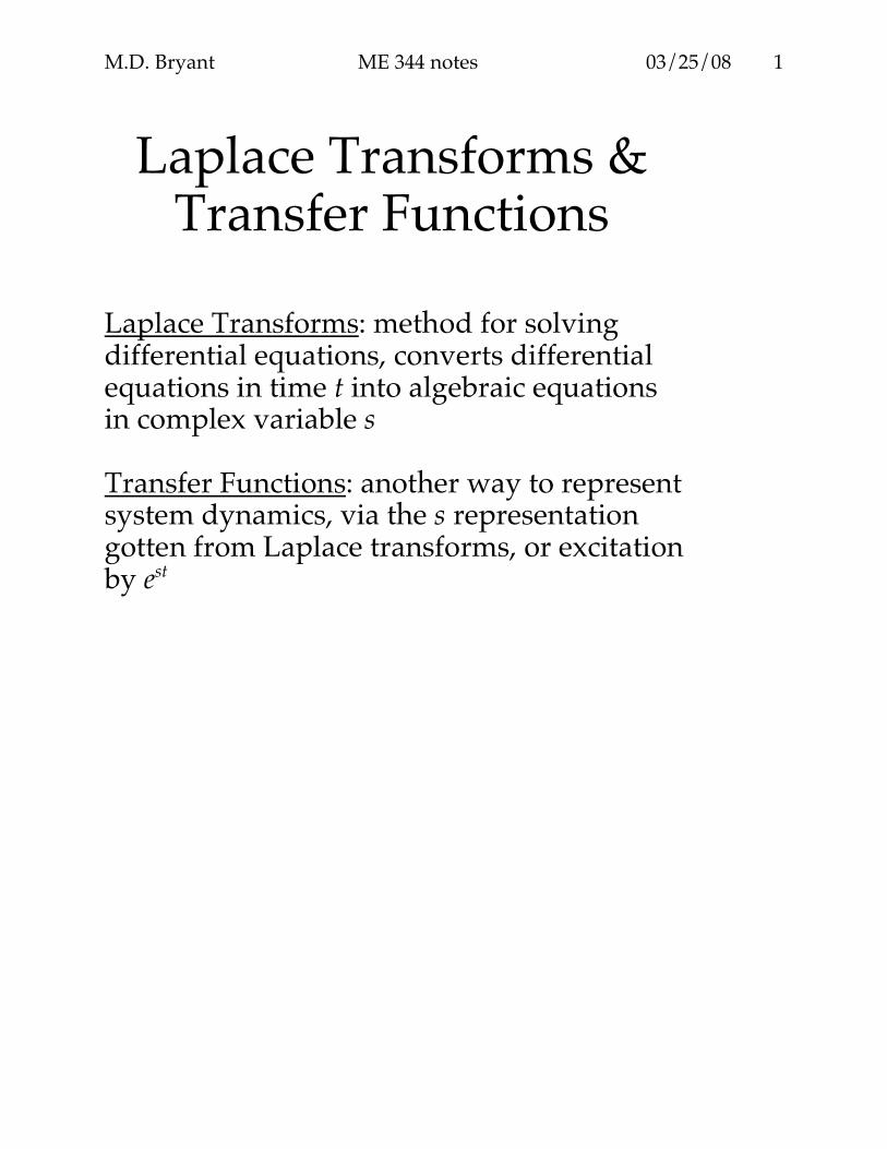
Laplace Transforms Purpose: Converts linear differential equation in t into algebraic equation in s

• Forward transform, t → s: f(t) ⇒ F(s)

F(s) = ⌡⌠

t= 0

∞ f(t) e- st dt = L {f(t); t → s }

Convergence/existence of integral: |f(t)| < M e- at , a + Re(s) > 0

so that e-[a + Re(s)]t finite as t → ∞

• Inverse transform, s→ t: F(s) ⇒ f(t)

f(t) = 12πj ⌡

⌠

ω= c- j∞

c+j∞ F(s) e st ds = L-1{F(s); s→ t }

Integral in complex plane, rarely do


3

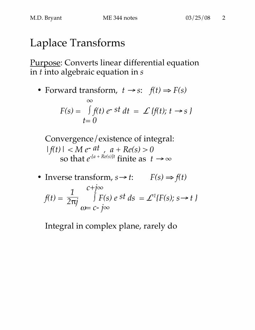
Procedure:

• Convert Linear Differential Equations

!

˙ x = Ax + f (t)

!

dn

x

dtn

+ an"1

dn"1

x

dtn"1

+!+ a2

d2

x

dt2+ a

1

d x

dt+ a

0x = f (t)

in time t into algebraic equations in complex variable s, via forward Laplace transforms:

X(s)=L {x(t); t → s }, F(s)=L {f(t); t → s }

• Solve resulting algebraic equations in s,

for solution X = X(s)

• Convert solution X(s) into time function x(t), via inverse Laplace transform:

x(t) = L-1{X(s); s→ t }


4

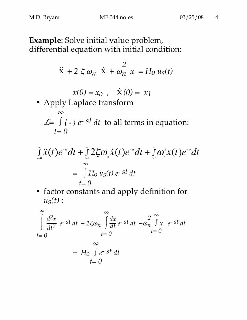
Example: Solve initial value problem, differential equation with initial condition:

x + 2 ζ ωn x + ω2n x = Ho us(t)

x(0) = xo , x (0) = x1

• Apply Laplace transform

L= ⌡⌠

t= 0

∞ { . } e- st dt to all terms in equation:

!

˙ x (t)e" st

t= 0

#

$ dt + 2%&n˙ x (t)e

" st

t= 0

#

$ dt + &n

2

x(t)e" st

dtt= 0

#

$

= ⌡⌠

t= 0

∞ Ho us(t) e- st dt

• factor constants and apply definition for us(t) :

⌡⌠

t= 0

∞

d2x

dt2 e- st dt + 2ζωn ⌡⌠

t= 0

∞ dxdt e- st dt +ω

2n ⌡⌠

t= 0

∞ x e- st dt

= Ho ⌡⌠

t= 0

∞ e- st dt


5

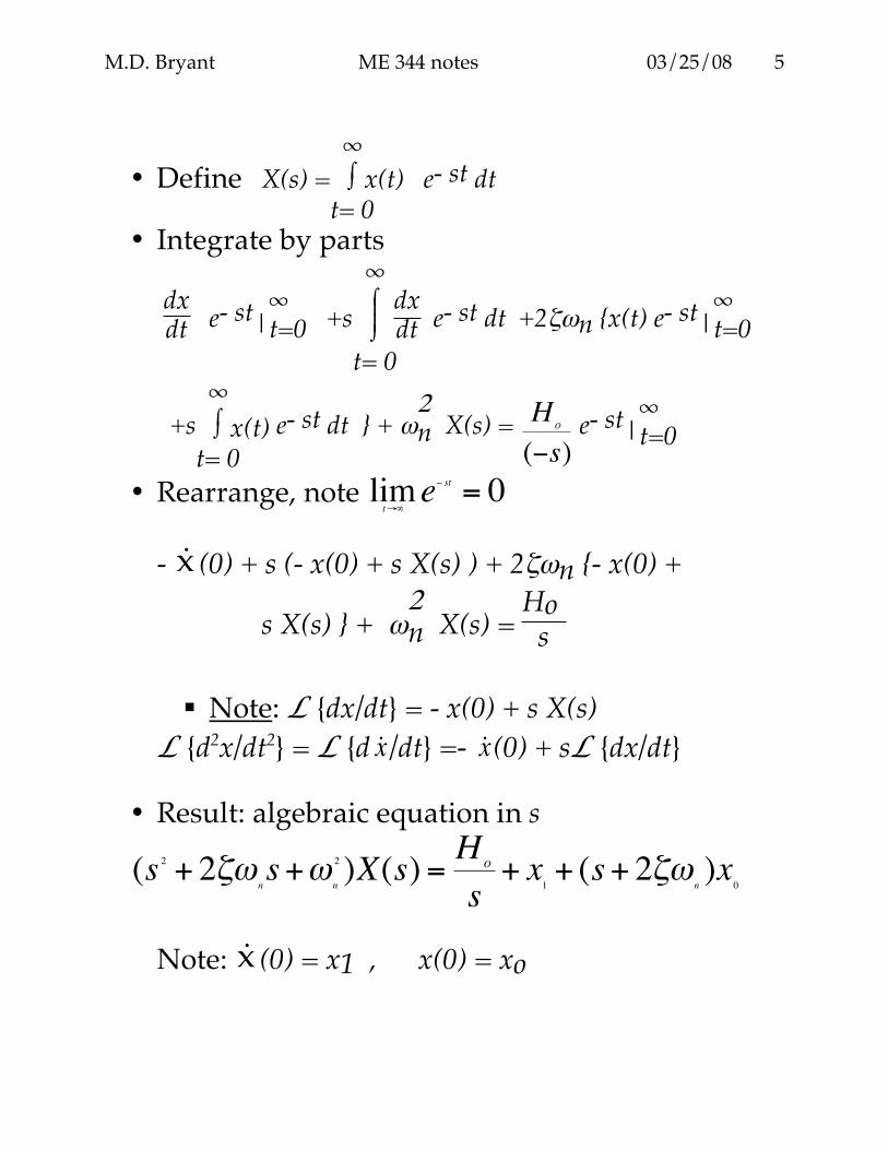
• Define X(s) = ⌡⌠

t= 0

∞ x(t) e- st dt

• Integrate by parts

dxdt e- st|

∞t=0 +s

⌡⌠

t= 0

∞

dxdt e- st dt +2ζωn {x(t) e- st|

∞t=0

+s ⌡⌠

t= 0

∞ x(t) e- st dt } + ω

2n X(s) =

!

HO

("s) e- st|

∞t=0

• Rearrange, note

!

limt"#e

$ st

= 0

- x (0) + s (- x(0) + s X(s) ) + 2ζωn {- x(0) +

s X(s) } + ω2n X(s) =

Ho s

Note: L {dx/dt} = - x(0) + s X(s)

L {d2x/dt2} = L {d

!

˙ x /dt} =-

!

˙ x (0) + sL {dx/dt}

• Result: algebraic equation in s

!

(s2

+ 2"#n

s+#n

2

)X(s) =H

O

s+ x

1+ (s+ 2"#

n

)x0

Note: x (0) = x1 , x(0) = xo


6

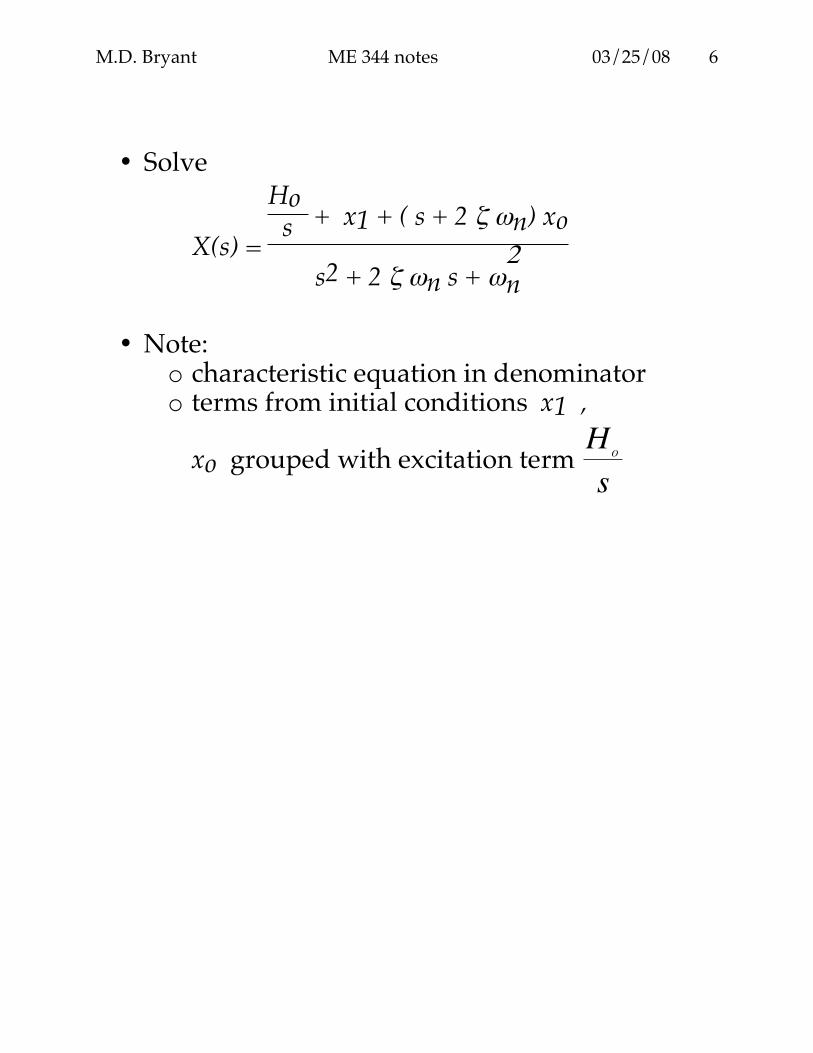
• Solve

X(s) =

Ho s + x1 + ( s + 2 ζ ωn) xo

s2 + 2 ζ ωn s + ω2n

• Note:

o characteristic equation in denominator o terms from initial conditions x1 ,

xo grouped with excitation term

!

HO

s


7

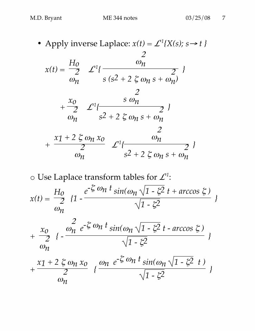
• Apply inverse Laplace: x(t) = L-1{X(s); s→ t }

x(t) = Ho

ω2n

L-1{ ω

2n

s (s2 + 2 ζ ωn s + ω2n)

}

+ xo

ω2n

L-1{s ω

2n

s2 + 2 ζ ωn s + ω2n

}

+ x1 + 2 ζ ωn xo

ω2n

L-1{ω

2n

s2 + 2 ζ ωn s + ω2n

}

o Use Laplace transform tables for L-1:

x(t) = Ho

ω2n

{1 - e-ζ ωn t sin(ωn 1 - ζ2 t + arccos ζ )

1 - ζ2 }

+ xo

ω2n

{ - ω

2n e-ζ ωn t sin(ωn 1 - ζ2 t - arccos ζ )

1 - ζ2 }

+ x1 + 2 ζ ωn xo

ω2n

{ ωn e-ζ ωn t sin(ωn 1 - ζ2 t )

1 - ζ2 }


8

Transfer Functions • Method to represent system dynamics, via

s representation from Laplace transforms. Transfer functions show flow of signal through a system, from input to output.

• Transfer function G(s) is ratio of output x

to input f, in s-domain (via Laplace trans.):

!

G(s) =X(s)

F(s) • Method gives system dynamics

representation equivalent to

Ordinary differential equations State equations

• Interchangeable: Can convert transfer function to differential equations


9

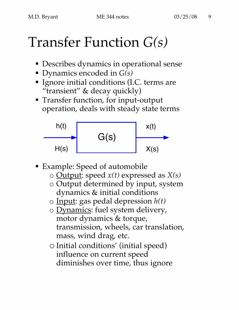
Transfer Function G(s) Describes dynamics in operational sense Dynamics encoded in G(s) Ignore initial conditions (I.C. terms are

“transient” & decay quickly) Transfer function, for input-output

operation, deals with steady state terms

h(t)

H(s)

x(t)

X(s)

G(s)

Example: Speed of automobile

o Output: speed x(t) expressed as X(s) o Output determined by input, system

dynamics & initial conditions o Input: gas pedal depression h(t) o Dynamics: fuel system delivery,

motor dynamics & torque, transmission, wheels, car translation, mass, wind drag, etc.

o Initial conditions’ (initial speed) influence on current speed diminishes over time, thus ignore


10

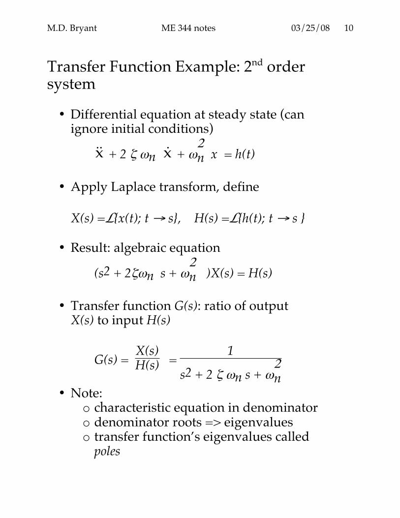
Transfer Function Example: 2nd order system

• Differential equation at steady state (can ignore initial conditions)

x + 2 ζ ωn x + ω2n x = h(t)

• Apply Laplace transform, define

X(s) =L{x(t); t → s}, H(s) =L{h(t); t → s }

• Result: algebraic equation

(s2 + 2ζωn s + ω2n )X(s) = H(s)

• Transfer function G(s): ratio of output

X(s) to input H(s)

G(s) = X(s)H(s) = 1

s2 + 2 ζ ωn s + ω2n

• Note: o characteristic equation in denominator o denominator roots => eigenvalues o transfer function’s eigenvalues called

poles


11

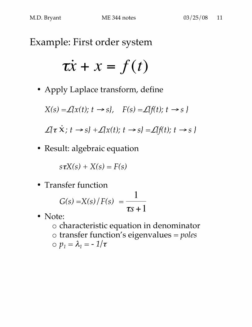
Example: First order system

!

"˙ x + x = f (t)

• Apply Laplace transform, define

X(s) =L{x(t); t → s}, F(s) =L{f(t); t → s }

L{τ x ; t → s} +L{x(t); t → s} =L{f(t); t → s }

• Result: algebraic equation sτX(s) + X(s) = F(s)

• Transfer function

G(s) =X(s)/F(s) =

!

1

"s+1

• Note: o characteristic equation in denominator o transfer function’s eigenvalues = poles o p1 = λ1 = - 1/τ


12

Transfer Function from State Equations

• Matrix form

!

˙ x = Ax + f (t)

• Explicit equation form

!

˙ x k= a

jkj=1

n

" xj+ f

k(t)

• Define

Xk(s)=L {xk(t); t → s }, Fk(s)=L {fk(t); t → s }

• Apply Laplace transform

!

sX(s) = AX(s)+F(s)

or

!

sXk(s) = a

jkj=1

n

" Xj(s)+F

k(s)


13

• Rearrange matrix form:

!

sI " A[ ]X(s) = F(s)

• Solve, via Cramer’s rule:

!

Xk(s) =

det sI " A[ ]kth column replaced by F ( s )

{ }det sI " A[ ]

• Transfer function, define which output

Xk(s) and which input Fj(s):

!

Gkj(s) =

Xk(s)

Fj(s)

• Solve, via previous result with all

components of F(s) zero, except Fj(s)


14

Example: differential equations from transfer function:

!

G(s) =X(s)

F(s)=

2s+ 5

s4

+ 3s3

+ 2s2

+ 2s+1

Cross multiply ratios:

!

s4 + 3s 3 + 2s 2 + 2s+1( )X(s) = 2s+ 5( )F(s)

!

s4

X + 3s3

X + 2s2

X + 2sX + X = 2sF + 5F Treat: s => d/dt

!

d4x

dt4

+ 3d3x

dt3

+ 2d2x

dt2

+ 2dx

dt+ x = 2

df

dt+ 5 f (t)


15

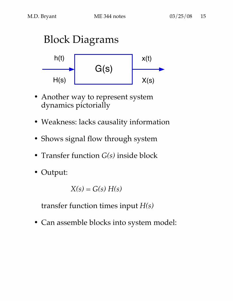
Block Diagrams

h(t)

H(s)

x(t)

X(s)

G(s)

• Another way to represent system dynamics pictorially

• Weakness: lacks causality information

• Shows signal flow through system

• Transfer function G(s) inside block

• Output:

X(s) = G(s) H(s)

transfer function times input H(s)

• Can assemble blocks into system model:


16

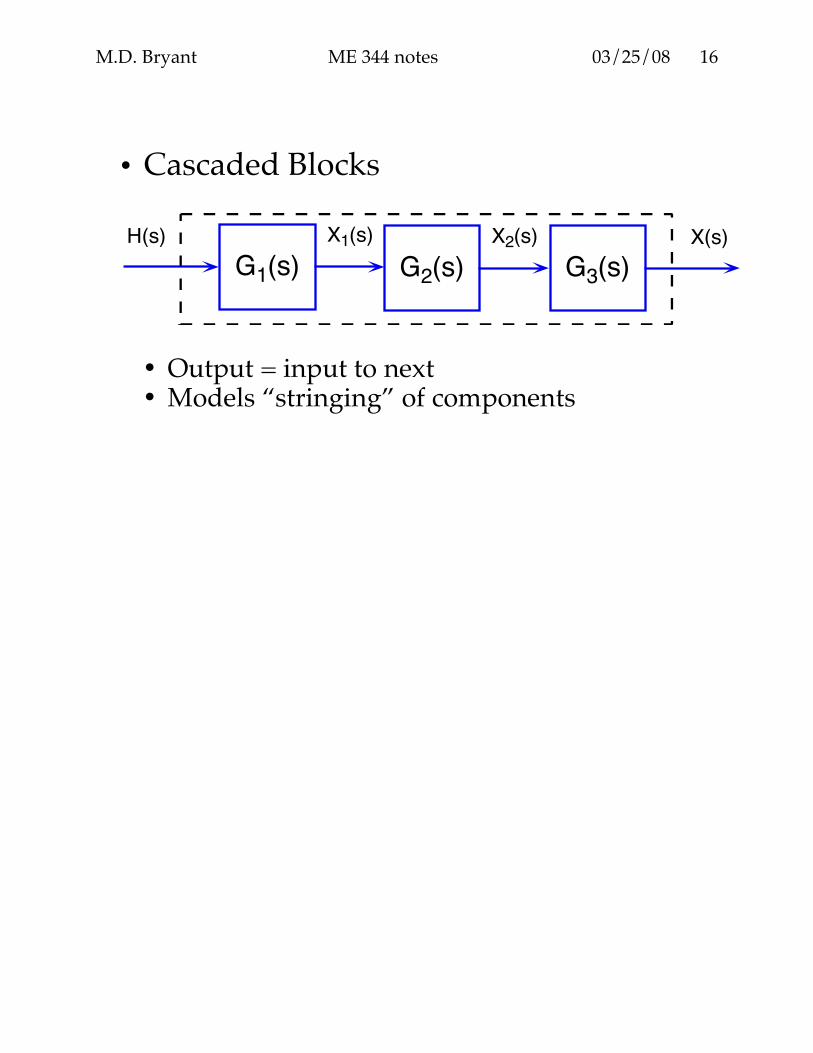
• Cascaded Blocks

H(s) X1(s)

G1(s)X2(s)

G2(s)X(s)

G3(s)

• Output = input to next • Models “stringing” of components


17

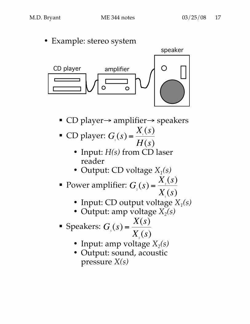
• Example: stereo system

CD player amplifier

speaker

CD player→ amplifier→ speakers

CD player:

!

G1(s) =

X1(s)

H (s)

• Input: H(s) from CD laser reader

• Output: CD voltage X1(s)

Power amplifier:

!

G2(s) =

X2(s)

X1(s)

• Input: CD output voltage X1(s) • Output: amp voltage X2(s)

Speakers:

!

G3(s) =

X(s)

X2(s)

• Input: amp voltage X2(s) • Output: sound, acoustic

pressure X(s)


18

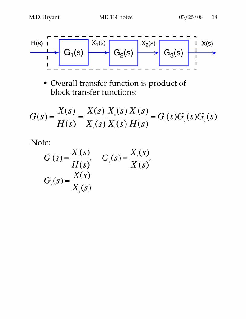
H(s) X1(s)

G1(s)X2(s)

G2(s)X(s)

G3(s)

• Overall transfer function is product of block transfer functions:

!

G(s) =X(s)

H (s)=X(s)

X2(s)

X2(s)

X1(s)

X1(s)

H (s)=G

1(s)G

2(s)G

3(s)

Note:

!

G1(s) =

X1(s)

H (s),

!

G2(s) =

X2(s)

X1(s)

,

!

G3(s) =

X(s)

X2(s)


19

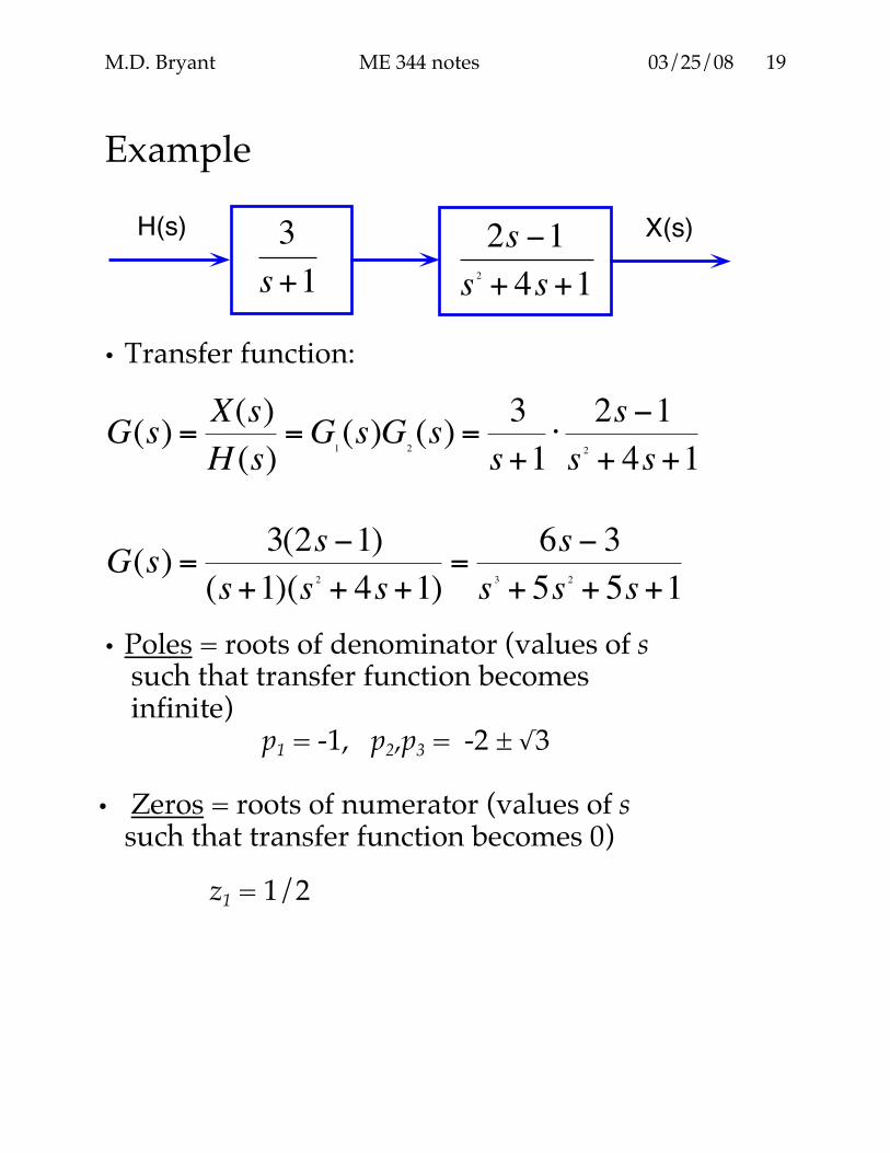
Example H(s) X(s)3

s+1

2s !1

s2

+ 4s+1

• Transfer function:

!

G(s) =X(s)

H (s)=G

1(s)G

2(s) =

3

s+1"2s #1

s2

+ 4s+1

!

G(s) =3(2s "1)

(s+1)(s2

+ 4s+1)=

6s " 3

s3

+ 5s2

+ 5s+1

• Poles = roots of denominator (values of s

such that transfer function becomes infinite)

p1 = -1, p2,p3 = -2 ± √3

• Zeros = roots of numerator (values of s such that transfer function becomes 0) z1 = 1/2


20

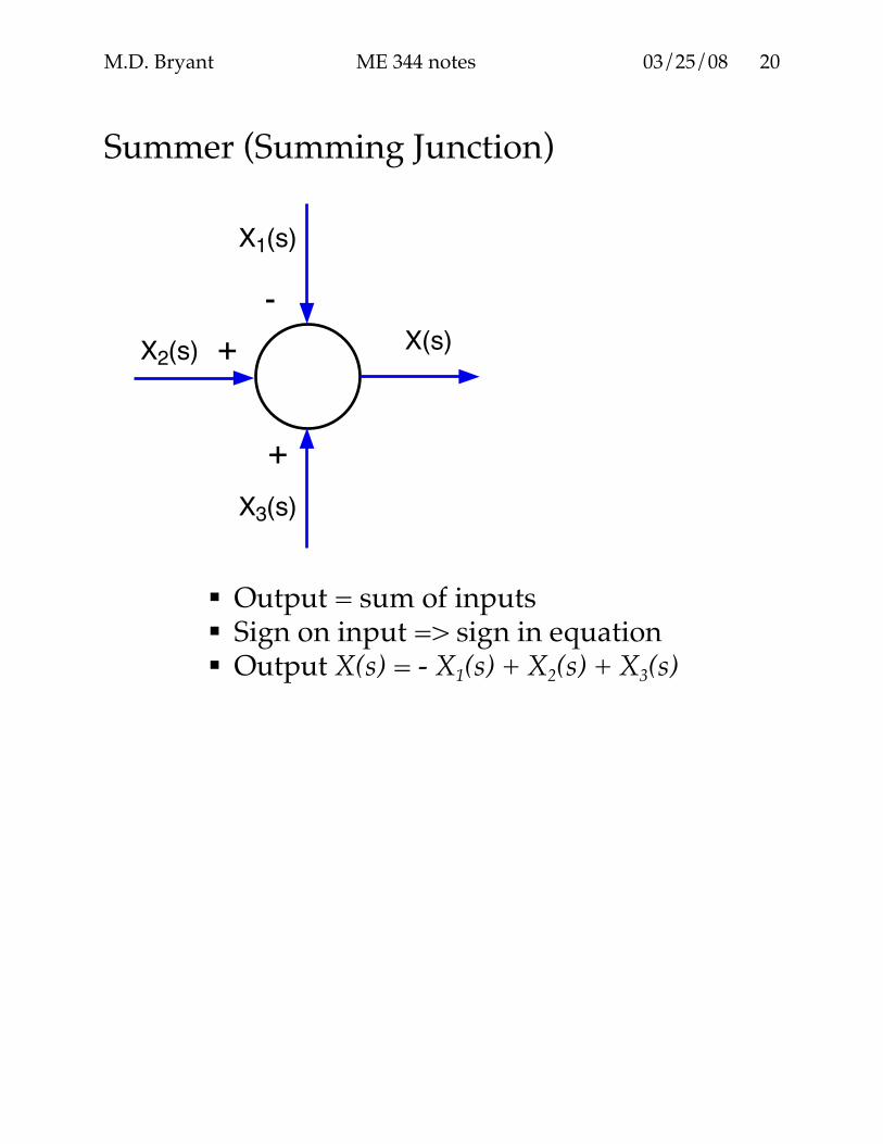
Summer (Summing Junction)

X1(s)

X2(s)X(s)+

+

-

X3(s)

Output = sum of inputs Sign on input => sign in equation Output X(s) = - X1(s) + X2(s) + X3(s)


21

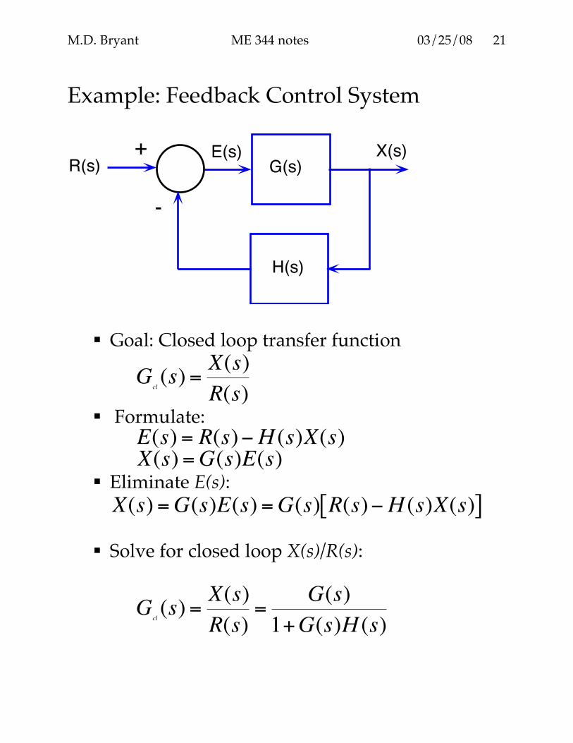
Example: Feedback Control System

R(s)X(s)

G(s)

H(s)

E(s)+

-

Goal: Closed loop transfer function

!

Gcl(s) =

X(s)

R(s)

Formulate:

!

E(s) = R(s)"H (s)X(s)

!

X(s) =G(s)E(s) Eliminate E(s):

!

X(s) =G(s)E(s) =G(s) R(s)"H (s)X(s)[ ]

Solve for closed loop X(s)/R(s):

!

Gcl(s) =

X(s)

R(s)=

G(s)

1+G(s)H (s)


22

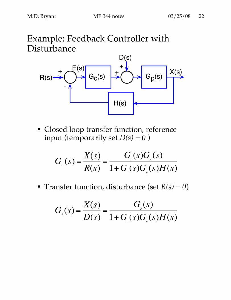
Example: Feedback Controller with Disturbance

Gc(s)R(s)X(s)

H(s)

E(s)+

-

Gp(s)++

D(s)

Closed loop transfer function, reference

input (temporarily set D(s) = 0 )

!

Gcl(s) =

X(s)

R(s)=

Gc(s)G

p(s)

1+Gc(s)G

p(s)H (s)

Transfer function, disturbance (set R(s) = 0)

!

Gd(s) =

X(s)

D(s)=

Gp(s)

1+Gc(s)G

p(s)H (s)


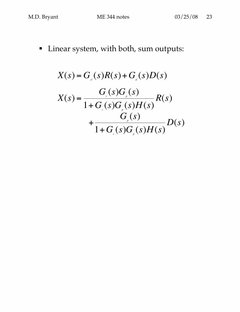
23

Linear system, with both, sum outputs:

!

X(s) =Gcl(s)R(s)+G

d(s)D(s)

!

X(s) =G

c(s)G

p(s)

1+Gc(s)G

p(s)H (s)

R(s)

!

+G

p(s)

1+Gc(s)G

p(s)H (s)

D(s)