Iterative Methodsfor Sparse
Linear Systems
Second Edition
0.10E-06
0.19E+07
Yousef Saad
Copyright c©2003 by the Society for Industrial and Applied Mathematics


Contents
Preface xiiiPreface to second edition. . . . . . . . . . . . . . . . . . . . . . . . . . . . . . . . . . xiiiPreface to first edition. . . . . . . . . . . . . . . . . . . . . . . . . . . . . . . . . . xix
1 Background in Linear Algebra 11.1 Matrices . . . . . . . . . . . . . . . . . . . . . . . . . . . . . 11.2 Square Matrices and Eigenvalues . . . . . . . . . . . . . . . . 31.3 Types of Matrices . . . . . . . . . . . . . . . . . . . . . . . . 41.4 Vector Inner Products and Norms . . . . . . . . . . . . . . . . 61.5 Matrix Norms . . . . . . . . . . . . . . . . . . . . . . . . . . 81.6 Subspaces, Range, and Kernel . . . . . . . . . . . . . . . . . . 101.7 Orthogonal Vectors and Subspaces . . . . . . . . . . . . . . . 111.8 Canonical Forms of Matrices . . . . . . . . . . . . . . . . . . 15
1.8.1 Reduction to the Diagonal Form . . . . . . . . . . 161.8.2 The Jordan Canonical Form . . . . . . . . . . . . 171.8.3 The Schur Canonical Form . . . . . . . . . . . . 171.8.4 Application to Powers of Matrices . . . . . . . . 20
1.9 Normal and Hermitian Matrices . . . . . . . . . . . . . . . . . 211.9.1 Normal Matrices . . . . . . . . . . . . . . . . . . 211.9.2 Hermitian Matrices . . . . . . . . . . . . . . . . 25
1.10 Nonnegative Matrices, M-Matrices . . . . . . . . . . . . . . . 271.11 Positive-Definite Matrices . . . . . . . . . . . . . . . . . . . . 321.12 Projection Operators . . . . . . . . . . . . . . . . . . . . . . . 34
1.12.1 Range and Null Space of a Projector . . . . . . . 341.12.2 Matrix Representations . . . . . . . . . . . . . . 361.12.3 Orthogonal and Oblique Projectors . . . . . . . . 371.12.4 Properties of Orthogonal Projectors . . . . . . . . 38
1.13 Basic Concepts in Linear Systems . . . . . . . . . . . . . . . . 391.13.1 Existence of a Solution . . . . . . . . . . . . . . 401.13.2 Perturbation Analysis . . . . . . . . . . . . . . . 41
2 Discretization of PDEs 472.1 Partial Differential Equations . . . . . . . . . . . . . . . . . . 47
2.1.1 Elliptic Operators . . . . . . . . . . . . . . . . . 47
v
vi CONTENTS
2.1.2 The Convection Diffusion Equation . . . . . . . . 502.2 Finite Difference Methods . . . . . . . . . . . . . . . . . . . . 50
2.2.1 Basic Approximations . . . . . . . . . . . . . . . 502.2.2 Difference Schemes for the Laplacean Operator . 522.2.3 Finite Differences for 1-D Problems . . . . . . . . 532.2.4 Upwind Schemes . . . . . . . . . . . . . . . . . 542.2.5 Finite Differences for 2-D Problems . . . . . . . . 562.2.6 Fast Poisson Solvers . . . . . . . . . . . . . . . . 58
2.3 The Finite Element Method . . . . . . . . . . . . . . . . . . . 622.4 Mesh Generation and Refinement . . . . . . . . . . . . . . . . 692.5 Finite Volume Method . . . . . . . . . . . . . . . . . . . . . . 69
3 Sparse Matrices 753.1 Introduction . . . . . . . . . . . . . . . . . . . . . . . . . . . 753.2 Graph Representations . . . . . . . . . . . . . . . . . . . . . . 76
3.2.1 Graphs and Adjacency Graphs . . . . . . . . . . . 773.2.2 Graphs of PDE Matrices . . . . . . . . . . . . . . 78
3.3 Permutations and Reorderings . . . . . . . . . . . . . . . . . . 793.3.1 Basic Concepts . . . . . . . . . . . . . . . . . . . 793.3.2 Relations with the Adjacency Graph . . . . . . . 813.3.3 Common Reorderings . . . . . . . . . . . . . . . 833.3.4 Irreducibility . . . . . . . . . . . . . . . . . . . . 91
3.4 Storage Schemes . . . . . . . . . . . . . . . . . . . . . . . . . 923.5 Basic Sparse Matrix Operations . . . . . . . . . . . . . . . . . 953.6 Sparse Direct Solution Methods . . . . . . . . . . . . . . . . . 96
3.6.1 Minimum degree ordering . . . . . . . . . . . . . 973.6.2 Nested Dissection ordering . . . . . . . . . . . . 97
3.7 Test Problems . . . . . . . . . . . . . . . . . . . . . . . . . . 98
4 Basic Iterative Methods 1054.1 Jacobi, Gauss-Seidel, and SOR . . . . . . . . . . . . . . . . . 105
4.1.1 Block Relaxation Schemes . . . . . . . . . . . . 1084.1.2 Iteration Matrices and Preconditioning . . . . . . 112
4.2 Convergence . . . . . . . . . . . . . . . . . . . . . . . . . . . 1144.2.1 General Convergence Result . . . . . . . . . . . . 1154.2.2 Regular Splittings . . . . . . . . . . . . . . . . . 1184.2.3 Diagonally Dominant Matrices . . . . . . . . . . 1194.2.4 Symmetric Positive Definite Matrices . . . . . . . 1224.2.5 Property A and Consistent Orderings . . . . . . . 123
4.3 Alternating Direction Methods . . . . . . . . . . . . . . . . . 127
5 Projection Methods 1335.1 Basic Definitions and Algorithms . . . . . . . . . . . . . . . . 133
5.1.1 General Projection Methods . . . . . . . . . . . . 134
CONTENTS vii
5.1.2 Matrix Representation . . . . . . . . . . . . . . . 1355.2 General Theory . . . . . . . . . . . . . . . . . . . . . . . . . 137
5.2.1 Two Optimality Results . . . . . . . . . . . . . . 1375.2.2 Interpretation in Terms of Projectors . . . . . . . 1385.2.3 General Error Bound . . . . . . . . . . . . . . . . 140
5.3 One-Dimensional Projection Processes . . . . . . . . . . . . . 1425.3.1 Steepest Descent . . . . . . . . . . . . . . . . . . 1425.3.2 Minimal Residual (MR) Iteration . . . . . . . . . 1455.3.3 Residual Norm Steepest Descent . . . . . . . . . 147
5.4 Additive and Multiplicative Processes . . . . . . . . . . . . . . 147
6 Krylov Subspace Methods Part I 1576.1 Introduction . . . . . . . . . . . . . . . . . . . . . . . . . . . 1576.2 Krylov Subspaces . . . . . . . . . . . . . . . . . . . . . . . . 1586.3 Arnoldi’s Method . . . . . . . . . . . . . . . . . . . . . . . . 160
6.3.1 The Basic Algorithm . . . . . . . . . . . . . . . . 1606.3.2 Practical Implementations . . . . . . . . . . . . . 162
6.4 Arnoldi’s Method for Linear Systems (FOM) . . . . . . . . . . 1656.4.1 Variation 1: Restarted FOM . . . . . . . . . . . . 1676.4.2 Variation 2: IOM and DIOM . . . . . . . . . . . 168
6.5 GMRES . . . . . . . . . . . . . . . . . . . . . . . . . . . . . 1716.5.1 The Basic GMRES Algorithm . . . . . . . . . . . 1726.5.2 The Householder Version . . . . . . . . . . . . . 1736.5.3 Practical Implementation Issues . . . . . . . . . . 1746.5.4 Breakdown of GMRES . . . . . . . . . . . . . . 1796.5.5 Variation 1: Restarting . . . . . . . . . . . . . . . 1796.5.6 Variation 2: Truncated GMRES Versions . . . . . 1806.5.7 Relations between FOM and GMRES . . . . . . . 1856.5.8 Residual smoothing . . . . . . . . . . . . . . . . 1906.5.9 GMRES for complex systems . . . . . . . . . . . 193
6.6 The Symmetric Lanczos Algorithm . . . . . . . . . . . . . . . 1946.6.1 The Algorithm . . . . . . . . . . . . . . . . . . . 1946.6.2 Relation with Orthogonal Polynomials . . . . . . 195
6.7 The Conjugate Gradient Algorithm . . . . . . . . . . . . . . . 1966.7.1 Derivation and Theory . . . . . . . . . . . . . . . 1966.7.2 Alternative Formulations . . . . . . . . . . . . . 2006.7.3 Eigenvalue Estimates from the CG Coefficients . . 201
6.8 The Conjugate Residual Method . . . . . . . . . . . . . . . . 2036.9 GCR, ORTHOMIN, and ORTHODIR . . . . . . . . . . . . . . 2046.10 The Faber-Manteuffel Theorem . . . . . . . . . . . . . . . . . 2066.11 Convergence Analysis . . . . . . . . . . . . . . . . . . . . . . 208
6.11.1 Real Chebyshev Polynomials . . . . . . . . . . . 2096.11.2 Complex Chebyshev Polynomials . . . . . . . . . 2106.11.3 Convergence of the CG Algorithm . . . . . . . . 214
viii CONTENTS
6.11.4 Convergence of GMRES . . . . . . . . . . . . . . 2156.12 Block Krylov Methods . . . . . . . . . . . . . . . . . . . . . 218
7 Krylov Subspace Methods Part II 2297.1 Lanczos Biorthogonalization . . . . . . . . . . . . . . . . . . 229
7.1.1 The Algorithm . . . . . . . . . . . . . . . . . . . 2297.1.2 Practical Implementations . . . . . . . . . . . . . 232
7.2 The Lanczos Algorithm for Linear Systems . . . . . . . . . . . 2347.3 The BCG and QMR Algorithms . . . . . . . . . . . . . . . . . 234
7.3.1 The Biconjugate Gradient Algorithm . . . . . . . 2347.3.2 Quasi-Minimal Residual Algorithm . . . . . . . . 236
7.4 Transpose-Free Variants . . . . . . . . . . . . . . . . . . . . . 2417.4.1 Conjugate Gradient Squared . . . . . . . . . . . . 2417.4.2 BICGSTAB . . . . . . . . . . . . . . . . . . . . 2447.4.3 Transpose-Free QMR (TFQMR) . . . . . . . . . 247
8 Methods Related to the Normal Equations 2598.1 The Normal Equations . . . . . . . . . . . . . . . . . . . . . . 2598.2 Row Projection Methods . . . . . . . . . . . . . . . . . . . . 261
8.2.1 Gauss-Seidel on the Normal Equations . . . . . . 2618.2.2 Cimmino’s Method . . . . . . . . . . . . . . . . 263
8.3 Conjugate Gradient and Normal Equations . . . . . . . . . . . 2668.3.1 CGNR . . . . . . . . . . . . . . . . . . . . . . . 2668.3.2 CGNE . . . . . . . . . . . . . . . . . . . . . . . 267
8.4 Saddle-Point Problems . . . . . . . . . . . . . . . . . . . . . . 268
9 Preconditioned Iterations 2759.1 Introduction . . . . . . . . . . . . . . . . . . . . . . . . . . . 2759.2 Preconditioned Conjugate Gradient . . . . . . . . . . . . . . . 276
9.2.1 Preserving Symmetry . . . . . . . . . . . . . . . 2769.2.2 Efficient Implementations . . . . . . . . . . . . . 279
9.3 Preconditioned GMRES . . . . . . . . . . . . . . . . . . . . . 2829.3.1 Left-Preconditioned GMRES . . . . . . . . . . . 2829.3.2 Right-Preconditioned GMRES . . . . . . . . . . 2849.3.3 Split Preconditioning . . . . . . . . . . . . . . . 2859.3.4 Comparison of Right and Left Preconditioning . . 285
9.4 Flexible Variants . . . . . . . . . . . . . . . . . . . . . . . . . 2879.4.1 Flexible GMRES . . . . . . . . . . . . . . . . . . 2879.4.2 DQGMRES . . . . . . . . . . . . . . . . . . . . 290
9.5 Preconditioned CG for the Normal Equations . . . . . . . . . . 2919.6 The Concus, Golub, and Widlund Algorithm . . . . . . . . . . 292
10 Preconditioning Techniques 29710.1 Introduction . . . . . . . . . . . . . . . . . . . . . . . . . . . 29710.2 Jacobi, SOR, and SSOR Preconditioners . . . . . . . . . . . . 298
CONTENTS ix
10.3 ILU Factorization Preconditioners . . . . . . . . . . . . . . . 30110.3.1 Incomplete LU Factorizations . . . . . . . . . . . 30110.3.2 Zero Fill-in ILU (ILU(0)) . . . . . . . . . . . . . 30710.3.3 Level of Fill and ILU(p) . . . . . . . . . . . . . . 31110.3.4 Matrices with Regular Structure . . . . . . . . . . 31510.3.5 Modified ILU (MILU) . . . . . . . . . . . . . . . 319
10.4 Threshold Strategies and ILUT . . . . . . . . . . . . . . . . . 32110.4.1 The ILUT Approach . . . . . . . . . . . . . . . . 32110.4.2 Analysis . . . . . . . . . . . . . . . . . . . . . . 32310.4.3 Implementation Details . . . . . . . . . . . . . . 32510.4.4 The ILUTP Approach . . . . . . . . . . . . . . . 32710.4.5 The ILUS Approach . . . . . . . . . . . . . . . . 33010.4.6 The Crout ILU Approach . . . . . . . . . . . . . 332
10.5 Approximate Inverse Preconditioners . . . . . . . . . . . . . . 33610.5.1 Approximating the Inverse of a Sparse Matrix . . 33710.5.2 Global Iteration . . . . . . . . . . . . . . . . . . 33710.5.3 Column-Oriented Algorithms . . . . . . . . . . . 33910.5.4 Theoretical Considerations . . . . . . . . . . . . 34110.5.5 Convergence of Self Preconditioned MR . . . . . 34310.5.6 Approximate Inverses via bordering . . . . . . . . 34610.5.7 Factored inverses via orthogonalization: AINV . . 34810.5.8 Improving a Preconditioner . . . . . . . . . . . . 349
10.6 Reordering for ILU . . . . . . . . . . . . . . . . . . . . . . . 35010.6.1 Symmetric permutations . . . . . . . . . . . . . . 35010.6.2 Nonsymmetric reorderings . . . . . . . . . . . . . 352
10.7 Block Preconditioners . . . . . . . . . . . . . . . . . . . . . . 35410.7.1 Block-Tridiagonal Matrices . . . . . . . . . . . . 35410.7.2 General Matrices . . . . . . . . . . . . . . . . . . 356
10.8 Preconditioners for the Normal Equations . . . . . . . . . . . 35610.8.1 Jacobi, SOR, and Variants . . . . . . . . . . . . . 35710.8.2 IC(0) for the Normal Equations . . . . . . . . . . 35710.8.3 Incomplete Gram-Schmidt and ILQ . . . . . . . . 360
11 Parallel Implementations 36911.1 Introduction . . . . . . . . . . . . . . . . . . . . . . . . . . . 36911.2 Forms of Parallelism . . . . . . . . . . . . . . . . . . . . . . . 370
11.2.1 Multiple Functional Units . . . . . . . . . . . . . 37011.2.2 Pipelining . . . . . . . . . . . . . . . . . . . . . 37011.2.3 Vector Processors . . . . . . . . . . . . . . . . . 37111.2.4 Multiprocessing and Distributed Computing . . . 371
11.3 Types of Parallel Architectures . . . . . . . . . . . . . . . . . 37111.3.1 Shared Memory Computers . . . . . . . . . . . . 37211.3.2 Distributed Memory Architectures . . . . . . . . 374
11.4 Types of Operations . . . . . . . . . . . . . . . . . . . . . . . 376
x CONTENTS
11.5 Matrix-by-Vector Products . . . . . . . . . . . . . . . . . . . 37811.5.1 The CSR and CSC Formats . . . . . . . . . . . . 37811.5.2 Matvecs in the Diagonal Format . . . . . . . . . . 38011.5.3 The Ellpack-Itpack Format . . . . . . . . . . . . 38111.5.4 The Jagged Diagonal Format . . . . . . . . . . . 38211.5.5 The Case of Distributed Sparse Matrices . . . . . 383
11.6 Standard Preconditioning Operations . . . . . . . . . . . . . . 38611.6.1 Parallelism in Forward Sweeps . . . . . . . . . . 38611.6.2 Level Scheduling: the Case of 5-Point Matrices . 38711.6.3 Level Scheduling for Irregular Graphs . . . . . . 388
12 Parallel Preconditioners 39312.1 Introduction . . . . . . . . . . . . . . . . . . . . . . . . . . . 39312.2 Block-Jacobi Preconditioners . . . . . . . . . . . . . . . . . . 39412.3 Polynomial Preconditioners . . . . . . . . . . . . . . . . . . . 395
12.3.1 Neumann Polynomials . . . . . . . . . . . . . . . 39612.3.2 Chebyshev Polynomials . . . . . . . . . . . . . . 39712.3.3 Least-Squares Polynomials . . . . . . . . . . . . 40012.3.4 The Nonsymmetric Case . . . . . . . . . . . . . . 403
12.4 Multicoloring . . . . . . . . . . . . . . . . . . . . . . . . . . 40612.4.1 Red-Black Ordering . . . . . . . . . . . . . . . . 40612.4.2 Solution of Red-Black Systems . . . . . . . . . . 40712.4.3 Multicoloring for General Sparse Matrices . . . . 408
12.5 Multi-Elimination ILU . . . . . . . . . . . . . . . . . . . . . . 40912.5.1 Multi-Elimination . . . . . . . . . . . . . . . . . 41012.5.2 ILUM . . . . . . . . . . . . . . . . . . . . . . . 412
12.6 Distributed ILU and SSOR . . . . . . . . . . . . . . . . . . . 41412.7 Other Techniques . . . . . . . . . . . . . . . . . . . . . . . . 417
12.7.1 Approximate Inverses . . . . . . . . . . . . . . . 41712.7.2 Element-by-Element Techniques . . . . . . . . . 41712.7.3 Parallel Row Projection Preconditioners . . . . . 419
13 Multigrid Methods 42313.1 Introduction . . . . . . . . . . . . . . . . . . . . . . . . . . . 42313.2 Matrices and spectra of model problems . . . . . . . . . . . . 424
13.2.1 Richardson’s iteration . . . . . . . . . . . . . . . 42813.2.2 Weighted Jacobi iteration . . . . . . . . . . . . . 43113.2.3 Gauss-Seidel iteration . . . . . . . . . . . . . . . 432
13.3 Inter-grid operations . . . . . . . . . . . . . . . . . . . . . . . 43613.3.1 Prolongation . . . . . . . . . . . . . . . . . . . . 43613.3.2 Restriction . . . . . . . . . . . . . . . . . . . . . 438
13.4 Standard multigrid techniques . . . . . . . . . . . . . . . . . . 43913.4.1 Coarse problems and smoothers . . . . . . . . . . 43913.4.2 Two-grid cycles . . . . . . . . . . . . . . . . . . 441
13.4.3 V-cycles and W-cycles . . . . . . . . . . . . . . . 44313.4.4 Full Multigrid . . . . . . . . . . . . . . . . . . . 447
13.5 Analysis for the two-grid cycle . . . . . . . . . . . . . . . . . 45113.5.1 Two important subspaces . . . . . . . . . . . . . 45113.5.2 Convergence analysis . . . . . . . . . . . . . . . 453
13.6 Algebraic Multigrid . . . . . . . . . . . . . . . . . . . . . . . 45513.6.1 Smoothness in AMG . . . . . . . . . . . . . . . . 45613.6.2 Interpolation in AMG . . . . . . . . . . . . . . . 45713.6.3 Defining coarse spaces in AMG . . . . . . . . . . 46013.6.4 AMG via Multilevel ILU . . . . . . . . . . . . . 461
13.7 Multigrid vs Krylov methods . . . . . . . . . . . . . . . . . . 464
14 Domain Decomposition Methods 46914.1 Introduction . . . . . . . . . . . . . . . . . . . . . . . . . . . 469
14.1.1 Notation . . . . . . . . . . . . . . . . . . . . . . 47014.1.2 Types of Partitionings . . . . . . . . . . . . . . . 47214.1.3 Types of Techniques . . . . . . . . . . . . . . . . 472
14.2 Direct Solution and the Schur Complement . . . . . . . . . . . 47414.2.1 Block Gaussian Elimination . . . . . . . . . . . . 47414.2.2 Properties of the Schur Complement . . . . . . . 47514.2.3 Schur Complement for Vertex-Based Partitionings 47614.2.4 Schur Complement for Finite-Element Partitionings 47914.2.5 Schur Complement for the model problem . . . . 481
14.3 Schwarz Alternating Procedures . . . . . . . . . . . . . . . . . 48414.3.1 Multiplicative Schwarz Procedure . . . . . . . . . 48414.3.2 Multiplicative Schwarz Preconditioning . . . . . . 48914.3.3 Additive Schwarz Procedure . . . . . . . . . . . . 49114.3.4 Convergence . . . . . . . . . . . . . . . . . . . . 492
14.4 Schur Complement Approaches . . . . . . . . . . . . . . . . . 49714.4.1 Induced Preconditioners . . . . . . . . . . . . . . 49714.4.2 Probing . . . . . . . . . . . . . . . . . . . . . . . 50014.4.3 Preconditioning Vertex-Based Schur Complements 500
14.5 Full Matrix Methods . . . . . . . . . . . . . . . . . . . . . . . 50114.6 Graph Partitioning . . . . . . . . . . . . . . . . . . . . . . . . 504
14.6.1 Basic Definitions . . . . . . . . . . . . . . . . . . 50414.6.2 Geometric Approach . . . . . . . . . . . . . . . . 50514.6.3 Spectral Techniques . . . . . . . . . . . . . . . . 50614.6.4 Graph Theory Techniques . . . . . . . . . . . . . 507
References 514
Index 535

xii CONTENTS
Preface to the second edition
In the six years that passed since the publication of the first edition of this book,iterative methods for linear systems have made good progress in scientific and engi-neering disciplines. This is due in great part to the increased complexity andsize ofthe new generation of linear and nonlinear systems which arise from typicalappli-cations. At the same time, parallel computing has penetrated the same applicationareas, as inexpensive computer power became broadly available and standard com-munication languages such as MPI gave a much needed standardization. This hascreated an incentive to utilize iterative rather than direct solvers becausethe prob-lems solved are typically from 3-dimensional models for which direct solversoftenbecome ineffective. Another incentive is that iterative methods are far easier to im-plement on parallel computers,
Though iterative methods for linear systems have seen a significant maturation,there are still many open problems. In particular, it still cannot be stated thatanarbitrary sparse linear system can be solved iteratively in an efficient way. If physicalinformation about the problem can be exploited, more effective and robust methodscan be tailored for the solutions. This strategy is exploited by multigrid methods. Inaddition, parallel computers necessitate different ways of approachingthe problemand solution algorithms that are radically different from classical ones.
Several new texts on the subject of this book have appeared since the first edition.Among these, are the books by Greenbaum [154], and Meurant [209]. The exhaustive5-volume treatise by G. W. Stewart [274] is likely to become the de-facto referencein numerical linear algebra in years to come. The related multigrid literature hasalso benefited from a few notable additions, including a new edition of the excellent“Multigrid tutorial” [65], and a new title by Trottenberg et al. [286].
Most notable among the changes from the first edition, is the addition of a sorelyneeded chapter on Multigrid techniques. The chapters which have seen the biggestchanges are Chapter 3, 6, 10, and 12. In most cases, the modifications were made toupdate the material by adding topics that were developed recently or gainedimpor-tance in the last few years. In some instances some of the older topics were removedor shortened. For example the discussion on parallel architecture has been short-ened. In the mid-1990’s hypercubes and “fat-trees” were important topic to teach.This is no longer the case, since manufacturers have taken steps to hide thetopologyfrom the user, in the sense that communication has become much less sensitiveto the
xiii
xiv PREFACE
underlying architecture.The bibliography has been updated to include work that has appeared in the last
few years, as well as to reflect change of emphasis when new topics have gainedimportance. Similarly, keeping in mind the educational side of this book, manynew exercises have been added. The first edition suffered many typographical errorswhich have been corrected. Many thanks to those readers who took the timeto pointout errors.
I would like to reiterate my thanks to all my colleagues who helped make thethe first edition a success (see the preface to the first edition). I received supportand encouragement from many students and colleagues to put together thisrevisedvolume. I also wish to thank those who proofread this book. I found that one ofthe best way to improve clarity is to solicit comments and questions from studentsin a course which teaches the material. Thanks to all students in Csci 8314 whohelped in this regard. Special thanks to Bernie Sheeham, who pointed out quite afew typographical errors and made numerous helpful suggestions.
My sincere thanks to Michele Benzi, Howard Elman, and Steve Mc Cormickfor their reviews of this edition. Michele proof-read a few chapters thoroughly andcaught a few misstatements. Steve Mc Cormick’s review of Chapter 13 helpedensurethat my slight bias for Krylov methods (versus multigrid) was not too obvious.Hiscomments were at the origin of the addition of Section 13.7 (Multigrid vs Krylovmethods).
I would also like to express my appreciation to the SIAM staff, especially LindaThiel and Sara Murphy.

PREFACE xv
Suggestions for teaching
This book can be used as a text to teach a graduate-level course on iterative methodsfor linear systems. Selecting topics to teach depends on whether the courseis taughtin a mathematics department or a computer science (or engineering) department, andwhether the course is over a semester or a quarter. Here are a few comments on therelevance of the topics in each chapter.
For a graduate course in a mathematics department, much of the material inChapter 1 should be known already. For non-mathematics majors most of the chap-ter must be covered or reviewed to acquire a good background for laterchapters.The important topics for the rest of the book are in Sections: 1.8.1, 1.8.3, 1.8.4, 1.9,1.11. Section 1.12 is best treated at the beginning of Chapter 5. Chapter 2 isessen-tially independent from the rest and could be skipped altogether in a quarter session,unless multigrid methods are to be included in the course. One lecture on finite dif-ferences and the resulting matrices would be enough for a non-math course. Chapter3 aims at familiarizing the student with some implementation issues associated withiterative solution procedures for general sparse matrices. In a computer science orengineering department, this can be very relevant. For mathematicians, a mentionof the graph theory aspects of sparse matrices and a few storage schemes may besufficient. Most students at this level should be familiar with a few of the elementaryrelaxation techniques covered in Chapter 4. The convergence theory can be skippedfor non-math majors. These methods are now often used as preconditioners and thismay be the only motive for covering them.
Chapter 5 introduces key concepts and presents projection techniques ingen-eral terms. Non-mathematicians may wish to skip Section 5.2.3. Otherwise, it isrecommended to start the theory section by going back to Section 1.12 on generaldefinitions on projectors. Chapters 6 and 7 represent the heart of the matter. It isrecommended to describe the first algorithms carefully and put emphasis on the factthat they generalize the one-dimensional methods covered in Chapter 5. Itis alsoimportant to stress the optimality properties of those methods in Chapter 6 and thefact that these follow immediately from the properties of projectors seen in Section1.12. Chapter 6 is rather long and the instructor will need to select what to coveramong the non-essential topics as well as topics for reading.
When covering the algorithms in Chapter 7, it is crucial to point out the maindifferences between them and those seen in Chapter 6. The variants such as CGS,BICGSTAB, and TFQMR can be covered in a short time, omitting details of thealgebraic derivations or covering only one of the three. The class of methods basedon the normal equation approach, i.e., Chapter 8, can be skipped in a math-orientedcourse, especially in the case of a quarter system. For a semester course, selectedtopics may be Sections 8.1, 8.2, and 8.4.
Preconditioning is known to be the determining ingredient in the success of iter-ative methods in solving real-life problems. Therefore, at least some partsof Chapter9 and Chapter 10 should be covered. Section 9.2 and (very briefly) 9.3 are recom-mended. From Chapter 10, discuss the basic ideas in Sections 10.1 through10.3.
xvi PREFACE
The rest could be skipped in a quarter course.Chapter 11 may be useful to present to computer science majors, but may be
skimmed through or skipped in a mathematics or an engineering course. Parts ofChapter 12 could be taught primarily to make the students aware of the importanceof “alternative” preconditioners. Suggested selections are: 12.2, 12.4, and 12.7.2 (forengineers).
Chapters 13 and 14 present important research areas and are primarilygearedto mathematics majors. Computer scientists or engineers may cover this material inless detail.
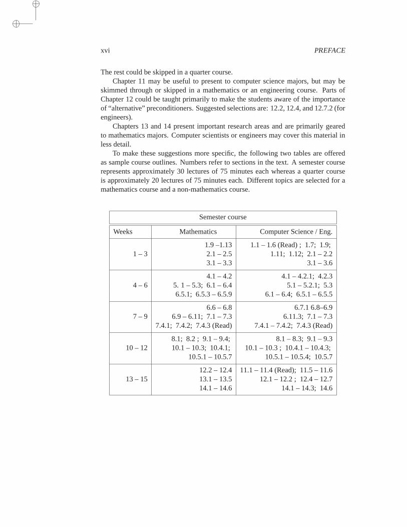
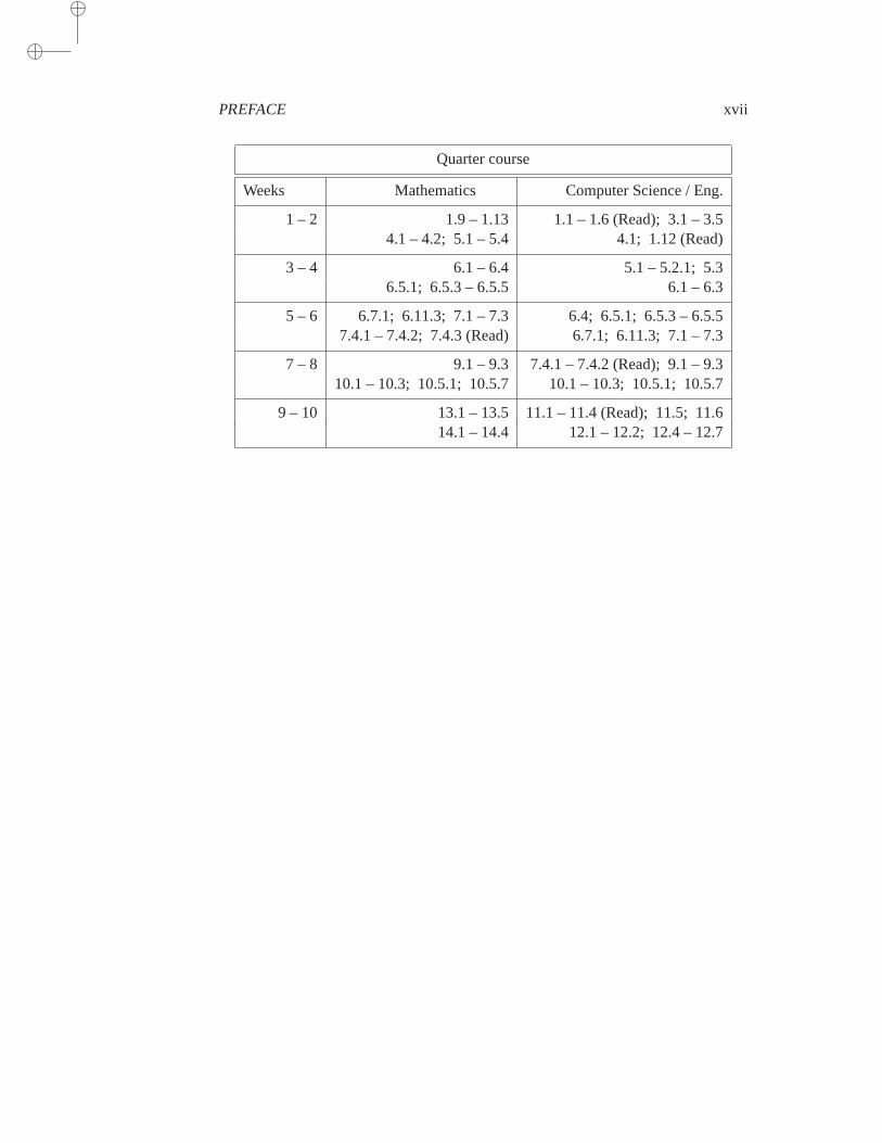
To make these suggestions more specific, the following two tables are offeredas sample course outlines. Numbers refer to sections in the text. A semester courserepresents approximately 30 lectures of 75 minutes each whereas a quarter courseis approximately 20 lectures of 75 minutes each. Different topics are selected for amathematics course and a non-mathematics course.
Semester course
Weeks Mathematics Computer Science / Eng.
1.9 –1.13 1.1 – 1.6 (Read) ; 1.7; 1.9;1 – 3 2.1 – 2.5 1.11; 1.12; 2.1 – 2.2
3.1 – 3.3 3.1 – 3.6
4.1 – 4.2 4.1 – 4.2.1; 4.2.34 – 6 5. 1 – 5.3; 6.1 – 6.4 5.1 – 5.2.1; 5.3
6.5.1; 6.5.3 – 6.5.9 6.1 – 6.4; 6.5.1 – 6.5.5
6.6 – 6.8 6.7.1 6.8–6.97 – 9 6.9 – 6.11; 7.1 – 7.3 6.11.3; 7.1 – 7.3
7.4.1; 7.4.2; 7.4.3 (Read) 7.4.1 – 7.4.2; 7.4.3 (Read)
8.1; 8.2 ; 9.1 – 9.4; 8.1 – 8.3; 9.1 – 9.310 – 12 10.1 – 10.3; 10.4.1; 10.1 – 10.3 ; 10.4.1 – 10.4.3;
10.5.1 – 10.5.7 10.5.1 – 10.5.4; 10.5.7
12.2 – 12.4 11.1 – 11.4 (Read); 11.5 – 11.613 – 15 13.1 – 13.5 12.1 – 12.2 ; 12.4 – 12.7
14.1 – 14.6 14.1 – 14.3; 14.6
PREFACE xvii
Quarter course
Weeks Mathematics Computer Science / Eng.
1 – 2 1.9 – 1.13 1.1 – 1.6 (Read); 3.1 – 3.54.1 – 4.2; 5.1 – 5.4 4.1; 1.12 (Read)
3 – 4 6.1 – 6.4 5.1 – 5.2.1; 5.36.5.1; 6.5.3 – 6.5.5 6.1 – 6.3
5 – 6 6.7.1; 6.11.3; 7.1 – 7.3 6.4; 6.5.1; 6.5.3 – 6.5.57.4.1 – 7.4.2; 7.4.3 (Read) 6.7.1; 6.11.3; 7.1 – 7.3
7 – 8 9.1 – 9.3 7.4.1 – 7.4.2 (Read); 9.1 – 9.310.1 – 10.3; 10.5.1; 10.5.7 10.1 – 10.3; 10.5.1; 10.5.7
9 – 10 13.1 – 13.5 11.1 – 11.4 (Read); 11.5; 11.614.1 – 14.4 12.1 – 12.2; 12.4 – 12.7

xviii PREFACE
Preface to the first edition
Iterative methods for solving general, large sparse linear systems have been gain-ing popularity in many areas of scientific computing. Until recently, direct solutionmethods were often preferred to iterative methods in real applications because oftheir robustness and predictable behavior. However, a number of efficient iterativesolvers were discovered and the increased need for solving very large linear systemstriggered a noticeable and rapid shift toward iterative techniques in many applica-tions.
This trend can be traced back to the 1960s and 1970s when two important de-velopments revolutionized solution methods for large linear systems. First wastherealization that one can take advantage of “sparsity” to design special direct meth-ods that can be quite economical. Initiated by electrical engineers, these “directsparse solution methods” led to the development of reliable and efficient general--purpose direct solution software codes over the next three decades.Second wasthe emergence of preconditioned conjugate gradient-like methods for solving linearsystems. It was found that the combination of preconditioning and Krylov subspaceiterations could provide efficient and simple “general-purpose” procedures that couldcompete with direct solvers. Preconditioning involves exploiting ideas from sparsedirect solvers. Gradually, iterative methods started to approach the qualityof di-rect solvers. In earlier times, iterative methods were often special-purpose in nature.They were developed with certain applications in mind, and their efficiency relied onmany problem-dependent parameters.
Now, three-dimensional models are commonplace and iterative methods are al-most mandatory. The memory and the computational requirements for solving three-dimensional Partial Differential Equations, or two-dimensional ones involving manydegrees of freedom per point, may seriously challenge the most efficient direct solversavailable today. Also, iterative methods are gaining ground because they are easierto implement efficiently on high-performance computers than direct methods.
My intention in writing this volume is to provide up-to-date coverage of itera-tive methods for solving large sparse linear systems. I focused the book on practicalmethods that work for general sparse matrices rather than for any specific class ofproblems. It is indeed becoming important to embrace applications not necessar-ily governed by Partial Differential Equations, as these applications are on the rise.
xix
xx PREFACE
Apart from two recent volumes by Axelsson [14] and Hackbusch [163], few books oniterative methods have appeared since the excellent ones by Varga [293]. and laterYoung [322]. Since then, researchers and practitioners have achieved remarkableprogress in the development and use of effective iterative methods. Unfortunately,fewer elegant results have been discovered since the 1950s and 1960s. The field hasmoved in other directions. Methods have gained not only in efficiency but also inrobustness and in generality. The traditional techniques which required rather com-plicated procedures to determine optimal acceleration parameters have yielded to theparameter-free conjugate gradient class of methods.
The primary aim of this book is to describe some of the best techniques availabletoday, from both preconditioners and accelerators. One of the aims of thebook isto provide a good mix of theory and practice. It also addresses some of thecurrentresearch issues such as parallel implementations and robust preconditioners. Theemphasis is on Krylov subspace methods, currently the most practical and commongroup of techniques used in applications. Although there is a tutorial chapter thatcovers the discretization of Partial Differential Equations, the book is notbiasedtoward any specific application area. Instead, the matrices are assumed to be generalsparse, possibly irregularly structured.
The book has been structured in four distinct parts. The first part, Chapters 1 to 4,presents the basic tools. The second part, Chapters 5 to 8, presents projection meth-ods and Krylov subspace techniques. The third part, Chapters 9 and 10,discussespreconditioning. The fourth part, Chapters 11 to 13, discusses parallelimplementa-tions and parallel algorithms.
Acknowledgments
I am grateful to a number of colleagues who proofread or reviewed different ver-sions of the manuscript. Among them are Randy Bramley (University of Indianaat Bloomingtin), Xiao-Chuan Cai (University of Colorado at Boulder), Tony Chan(University of California at Los Angeles), Jane Cullum (IBM, YorktownHeights),Alan Edelman (Massachussett Institute of Technology), Paul Fischer (Brown Univer-sity), David Keyes (Old Dominion University), Beresford Parlett (University of Cali-fornia at Berkeley) and Shang-Hua Teng (University of Minnesota).Their numerouscomments, corrections, and encouragements were a highly appreciated contribution.In particular, they helped improve the presentation considerably and prompted theaddition of a number of topics missing from earlier versions.
This book evolved from several successive improvements of a set of lecture notesfor the course “Iterative Methods for Linear Systems” which I taught atthe Univer-sity of Minnesota in the last few years. I apologize to those students who used theearlier error-laden and incomplete manuscripts. Their input and criticism contributedsignificantly to improving the manuscript. I also wish to thank those students at MIT(with Alan Edelman) and UCLA (with Tony Chan) who used this book in manuscriptform and provided helpful feedback. My colleagues at the universityof Minnesota,staff and faculty members, have helped in different ways. I wish to thank inparticular

PREFACE xxi
Ahmed Sameh for his encouragements and for fostering a productive environment inthe department. Finally, I am grateful to the National Science Foundation fortheircontinued financial support of my research, part of which is represented in this work.
Yousef Saad

Chapter 1
BACKGROUND IN LINEAR ALGEBRA
This chapter gives an overview of the relevant concepts in linear algebra which are useful in
later chapters. It begins with a review of basic matrix theory and introduces the elementary
notation used throughout the book. The convergence analysis of iterative methods requires a
good level of knowledge in mathematical analysis and in linear algebra. Traditionally, many of the
concepts presented specifically for these analyses have been geared toward matrices arising from
the discretization of Partial Differential Equations and basic relaxation-type methods. These
concepts are now becoming less important because of the trend toward projection-type methods
which have more robust convergence properties and require different analysis tools. The material
covered in this chapter will be helpful in establishing some theory for the algorithms and defining
the notation used throughout the book.
1.1 Matrices
For the sake of generality, all vector spaces considered in this chapter are complex,unless otherwise stated. A complexn ×m matrixA is ann ×m array of complexnumbers
aij , i = 1, . . . , n, j = 1, . . . ,m.
The set of alln×mmatrices is a complex vector space denoted byCn×m. The main
operations with matrices are the following:
• Addition: C = A+B, whereA,B, andC are matrices of sizen×m and
cij = aij + bij , i = 1, 2, . . . n, j = 1, 2, . . .m.
• Multiplication by a scalar:C = αA, where
cij = α aij , i = 1, 2, . . . n, j = 1, 2, . . .m.
1
2 CHAPTER 1. BACKGROUND IN LINEAR ALGEBRA
• Multiplication by another matrix:
C = AB,
whereA ∈ Cn×m, B ∈ C
m×p, C ∈ Cn×p, and
cij =m∑
k=1
aikbkj .
Sometimes, a notation with column vectors and row vectors is used. The columnvectora∗j is the vector consisting of thej-th column ofA,
a∗j =
a1j
a2j...anj
.
Similarly, the notationai∗ will denote thei-th row of the matrixA
ai∗ = (ai1, ai2, . . . , aim) .
For example, the following could be written
A = (a∗1, a∗2, . . . , a∗m) ,
or
A =
a1∗a2∗..an∗
.
The transposeof a matrixA in Cn×m is a matrixC in C
m×n whose elementsare defined bycij = aji, i = 1, . . . ,m, j = 1, . . . , n. It is denoted byAT . It is oftenmore relevant to use thetranspose conjugatematrix denoted byAH and defined by
AH = AT = AT ,
in which the bar denotes the (element-wise) complex conjugation.Matrices are strongly related to linear mappings between vector spaces of finite
dimension. This is because they represent these mappings with respect to two givenbases: one for the initial vector space and the other for the image vector space, orrangeof A.

1.2. SQUARE MATRICES AND EIGENVALUES 3
1.2 Square Matrices and Eigenvalues
A matrix issquareif it has the same number of columns and rows, i.e., ifm = n. Animportant square matrix is the identity matrix
I = δiji,j=1,...,n,
whereδij is the Kronecker symbol. The identity matrix satisfies the equalityAI =IA = A for every matrixA of sizen. The inverse of a matrix, when it exists, is amatrixC such that
CA = AC = I.
The inverse ofA is denoted byA−1.Thedeterminantof a matrix may be defined in several ways. For simplicity, the
following recursive definition is used here. The determinant of a1× 1 matrix (a) isdefined as the scalara. Then the determinant of ann× n matrix is given by
det(A) =n∑
j=1
(−1)j+1a1jdet(A1j),
whereA1j is an(n− 1)× (n− 1) matrix obtained by deleting the first row and thej-th column ofA. A matrix is said to besingularwhendet(A) = 0 andnonsingularotherwise. We have the following simple properties:
• det(AB) = det(A)det(B).
• det(AT ) = det(A).
• det(αA) = αndet(A).
• det(A) = det(A).
• det(I) = 1.
From the above definition of determinants it can be shown by induction that thefunction that maps a given complex valueλ to the valuepA(λ) = det(A − λI)is a polynomial of degreen; see Exercise 8. This is known as thecharacteristicpolynomialof the matrixA.
Definition 1.1 A complex scalarλ is called an eigenvalue of the square matrixAif a nonzero vectoru of C
n exists such thatAu = λu. The vectoru is called aneigenvector ofA associated withλ. The set of all the eigenvalues ofA is called thespectrum ofA and is denoted byσ(A).
A scalarλ is an eigenvalue ofA if and only if det(A− λI) ≡ pA(λ) = 0. Thatis true if and only if (iff thereafter)λ is a root of the characteristic polynomial. Inparticular, there are at mostn distinct eigenvalues.
It is clear that a matrix is singular if and only if it admits zero as an eigenvalue.A well known result in linear algebra is stated in the following proposition.
4 CHAPTER 1. BACKGROUND IN LINEAR ALGEBRA
Proposition 1.2 A matrixA is nonsingular if and only if it admits an inverse.
Thus, the determinant of a matrix determines whether or not the matrix admits aninverse.
The maximum modulus of the eigenvalues is calledspectral radiusand is de-noted byρ(A)
ρ(A) = maxλ∈σ(A)
|λ|.
Thetraceof a matrix is equal to the sum of all its diagonal elements
tr(A) =n∑
i=1
aii.
It can be easily shown that the trace ofA is also equal to the sum of the eigenvaluesof A counted with their multiplicities as roots of the characteristic polynomial.
Proposition 1.3 If λ is an eigenvalue ofA, then λ is an eigenvalue ofAH . Aneigenvectorv of AH associated with the eigenvalueλ is called a left eigenvector ofA.
When a distinction is necessary, an eigenvector ofA is often called a right eigen-vector. Therefore, the eigenvalueλ as well as the right and left eigenvectors,u andv, satisfy the relations
Au = λu, vHA = λvH ,
or, equivalently,uHAH = λuH , AHv = λv.
1.3 Types of Matrices
The choice of a method for solving linear systems will often depend on the structureof the matrixA. One of the most important properties of matrices is symmetry, be-cause of its impact on the eigenstructure ofA. A number of other classes of matricesalso have particular eigenstructures. The most important ones are listed below:
• Symmetric matrices:AT = A.
• Hermitian matrices:AH = A.
• Skew-symmetric matrices:AT = −A.
• Skew-Hermitian matrices:AH = −A.
• Normal matrices:AHA = AAH .
• Nonnegative matrices:aij ≥ 0, i, j = 1, . . . , n (similar definition for non-positive, positive, and negative matrices).
1.3. TYPES OF MATRICES 5
• Unitary matrices:QHQ = I.
It is worth noting that a unitary matrixQ is a matrix whose inverse is its transposeconjugateQH , since
QHQ = I → Q−1 = QH . (1.1)
A matrixQ such thatQHQ is diagonal is often called orthogonal.Some matrices have particular structures that are often convenient for computa-
tional purposes. The following list, though incomplete, gives an idea of these specialmatrices which play an important role in numerical analysis and scientific computingapplications.
• Diagonal matrices:aij = 0 for j 6= i. Notation:
A = diag (a11, a22, . . . , ann) .
• Upper triangular matrices:aij = 0 for i > j.
• Lower triangular matrices:aij = 0 for i < j.
• Upper bidiagonal matrices:aij = 0 for j 6= i or j 6= i+ 1.
• Lower bidiagonal matrices:aij = 0 for j 6= i or j 6= i− 1.
• Tridiagonal matrices:aij = 0 for any pairi, j such that|j − i| > 1. Notation:
A = tridiag (ai,i−1, aii, ai,i+1) .
• Banded matrices:aij 6= 0 only if i−ml ≤ j ≤ i+mu, whereml andmu aretwo nonnegative integers. The numberml + mu + 1 is called the bandwidthof A.
• Upper Hessenberg matrices:aij = 0 for any pairi, j such thati > j + 1.Lower Hessenberg matrices can be defined similarly.
• Outer product matrices:A = uvH , where bothu andv are vectors.
• Permutation matrices:the columns ofA are a permutation of the columns ofthe identity matrix.
• Block diagonal matrices:generalizes the diagonal matrix by replacing eachdiagonal entry by a matrix. Notation:
A = diag (A11, A22, . . . , Ann) .
• Block tridiagonal matrices:generalizes the tridiagonal matrix by replacingeach nonzero entry by a square matrix. Notation:
A = tridiag (Ai,i−1, Aii, Ai,i+1) .
The above properties emphasize structure, i.e., positions of the nonzero elementswith respect to the zeros. Also, they assume that there are many zero elements orthat the matrix is of low rank. This is in contrast with the classifications listed earlier,such as symmetry or normality.
6 CHAPTER 1. BACKGROUND IN LINEAR ALGEBRA
1.4 Vector Inner Products and Norms
An inner product on a (complex) vector spaceX is any mappings from X × X intoC,
x ∈ X, y ∈ X → s(x, y) ∈ C,
which satisfies the following conditions:
1. s(x, y) is linear with respect tox, i.e.,
s(λ1x1 + λ2x2, y) = λ1s(x1, y) + λ2s(x2, y), ∀ x1, x2 ∈ X,∀ λ1, λ2 ∈ C.
2. s(x, y) is Hermitian, i.e.,
s(y, x) = s(x, y), ∀ x, y ∈ X.
3. s(x, y) is positive definite, i.e.,
s(x, x) > 0, ∀ x 6= 0.
Note that (2) implies thats(x, x) is real and therefore, (3) adds the constraint thats(x, x) must also be positive for any nonzerox. For anyx andy,
s(x, 0) = s(x, 0.y) = 0.s(x, y) = 0.
Similarly, s(0, y) = 0 for anyy. Hence,s(0, y) = s(x, 0) = 0 for anyx andy. Inparticular the condition (3) can be rewritten as
s(x, x) ≥ 0 and s(x, x) = 0 iff x = 0,
as can be readily shown. A useful relation satisfied by any inner product is the so-called Cauchy-Schwartz inequality:
|s(x, y)|2 ≤ s(x, x) s(y, y). (1.2)
The proof of this inequality begins by expandings(x− λy, x− λy) using the prop-erties ofs,
s(x− λy, x− λy) = s(x, x)− λs(x, y)− λs(y, x) + |λ|2s(y, y).
If y = 0 then the inequality is trivially satisfied. Assume thaty 6= 0 and takeλ = s(x, y)/s(y, y). Then, from the above equality,s(x − λy, x − λy) ≥ 0 showsthat
0 ≤ s(x− λy, x− λy) = s(x, x)− 2|s(x, y)|2s(y, y)
+|s(x, y)|2s(y, y)
= s(x, x)− |s(x, y)|2
s(y, y),
1.4. VECTOR INNER PRODUCTS AND NORMS 7
which yields the result (1.2).In the particular case of the vector spaceX = C
n, a “canonical” inner productis theEuclidean inner product. The Euclidean inner product of two vectorsx =(xi)i=1,...,n andy = (yi)i=1,...,n of C
n is defined by
(x, y) =n∑
i=1
xiyi, (1.3)
which is often rewritten in matrix notation as
(x, y) = yHx. (1.4)
It is easy to verify that this mapping does indeed satisfy the three conditions requiredfor inner products, listed above. A fundamental property of the Euclidean innerproduct in matrix computations is the simple relation
(Ax, y) = (x,AHy), ∀ x, y ∈ Cn. (1.5)
The proof of this is straightforward. Theadjoint of A with respect to an arbitraryinner productis a matrixB such that(Ax, y) = (x,By) for all pairs of vectorsxandy. A matrix is self-adjoint, or Hermitian with respect to this inner product, if itis equal to its adjoint. The following proposition is a consequence of the equality(1.5).
Proposition 1.4 Unitary matrices preserve the Euclidean inner product, i.e.,
(Qx,Qy) = (x, y)
for any unitary matrixQ and any vectorsx andy.
Proof. Indeed,(Qx,Qy) = (x,QHQy) = (x, y).
A vector norm on a vector spaceX is a real-valued functionx → ‖x‖ on X,which satisfies the following three conditions:
1. ‖x‖ ≥ 0, ∀ x ∈ X, and ‖x‖ = 0 iff x = 0.
2. ‖αx‖ = |α|‖x‖, ∀ x ∈ X, ∀α ∈ C.
3. ‖x+ y‖ ≤ ‖x‖+ ‖y‖, ∀ x, y ∈ X.
For the particular case whenX = Cn, we can associate with the inner product
(1.3) theEuclidean normof a complex vector defined by
‖x‖2 = (x, x)1/2.
It follows from Proposition 1.4 that a unitary matrix preserves the Euclideannormmetric, i.e.,
‖Qx‖2 = ‖x‖2, ∀ x.
8 CHAPTER 1. BACKGROUND IN LINEAR ALGEBRA
The linear transformation associated with a unitary matrixQ is therefore anisometry.The most commonly used vector norms in numerical linear algebra are special
cases of the Holder norms
‖x‖p =
(n∑
i=1
|xi|p)1/p
. (1.6)
Note that the limit of‖x‖p whenp tends to infinity exists and is equal to the maxi-mum modulus of thexi’s. This defines a norm denoted by‖.‖∞. The casesp = 1,p = 2, andp =∞ lead to the most important norms in practice,
‖x‖1 = |x1|+ |x2|+ · · ·+ |xn|,‖x‖2 =
[|x1|2 + |x2|2 + · · ·+ |xn|2
]1/2,
‖x‖∞ = maxi=1,...,n
|xi|.
The Cauchy-Schwartz inequality of (1.2) becomes
|(x, y)| ≤ ‖x‖2‖y‖2.
1.5 Matrix Norms
For a general matrixA in Cn×m, we define the following special set of norms
‖A‖pq = maxx∈Cm, x 6=0
‖Ax‖p‖x‖q
. (1.7)
The norm‖.‖pq is inducedby the two norms‖.‖p and‖.‖q. These norms satisfy theusual properties of norms, i.e.,
‖A‖ ≥ 0, ∀ A ∈ Cn×m, and ‖A‖ = 0 iff A = 0 (1.8)
‖αA‖ = |α|‖A‖,∀ A ∈ Cn×m, ∀ α ∈ C (1.9)
‖A+B‖ ≤ ‖A‖+ ‖B‖, ∀ A,B ∈ Cn×m. (1.10)
(1.11)
A norm which satisfies the above three properties is nothing but avector normap-plied to the matrix considered as a vector consisting of them columns stacked into avector of sizenm.
The most important cases are again those associated withp, q = 1, 2,∞. Thecaseq = p is of particular interest and the associated norm‖.‖pq is simply denotedby ‖.‖p and called a “p-norm.” A fundamental property of ap-norm is that
‖AB‖p ≤ ‖A‖p‖B‖p,
an immediate consequence of the definition (1.7). Matrix norms that satisfy the aboveproperty are sometimes calledconsistent. Often a norm satisfying the properties

1.5. MATRIX NORMS 9
(1.8–1.10) and which is consistent is called amatrix norm. A result of consistency isthat for any square matrixA,
‖Ak‖p ≤ ‖A‖kp.In particular the matrixAk converges to zero ifanyof its p-norms is less than 1.
The Frobenius norm of a matrix is defined by
‖A‖F =
m∑
j=1
n∑
i=1
|aij |2
1/2
. (1.12)
This can be viewed as the 2-norm of the column (or row) vector inCn2
consistingof all the columns (respectively rows) ofA listed from1 tom (respectively1 to n.)It can be shown that this norm is also consistent, in spite of the fact that it is notinduced by a pair of vector norms, i.e., it is not derived from a formula of the form(1.7); see Exercise 5. However, it does not satisfy some of the other properties ofthep-norms. For example, the Frobenius norm of the identity matrix is not equal toone. To avoid these difficulties,we will only use the term matrix norm for a normthat is induced by two norms as in the definition (1.7). Thus, we will not considerthe Frobenius norm to be a proper matrix norm, according to our conventions, eventhough it is consistent.
The following equalities satisfied by the matrix norms defined above lead to al-ternative definitions that are often easier to work with:
‖A‖1 = maxj=1,...,m
n∑
i=1
|aij |, (1.13)
‖A‖∞ = maxi=1,...,n
m∑
j=1
|aij |, (1.14)
‖A‖2 =[ρ(AHA)
]1/2=[ρ(AAH)
]1/2, (1.15)
‖A‖F =[tr(AHA)
]1/2=[tr(AAH)
]1/2. (1.16)
As will be shown later, the eigenvalues ofAHA are nonnegative. Their squareroots are calledsingular valuesof A and are denoted byσi, i = 1, . . . ,m. Thus, therelation (1.15) states that‖A‖2 is equal toσ1, the largest singular value ofA.
Example 1.1. From the relation (1.15), it is clear that the spectral radiusρ(A) isequal to the 2-norm of a matrix when the matrix is Hermitian. However, it is nota matrix norm in general. For example, the first property of norms is not satisfied,since for
A =
(0 10 0
)
,
we haveρ(A) = 0 whileA 6= 0. Also, the triangle inequality is not satisfied for thepairA, andB = AT whereA is defined above. Indeed,
ρ(A+B) = 1 while ρ(A) + ρ(B) = 0.
10 CHAPTER 1. BACKGROUND IN LINEAR ALGEBRA
1.6 Subspaces, Range, and Kernel
A subspace ofCn is a subset ofCn that is also a complex vector space. The set ofall linear combinations of a set of vectorsG = a1, a2, . . . , aq of C
n is a vectorsubspace called the linear span ofG,
spanG = span a1, a2, . . . , aq
=
z ∈ Cn
∣∣∣∣z =
q∑
i=1
αiai; αii=1,...,q ∈ Cq
.
If the ai’s are linearly independent, then each vector ofspanG admits a uniqueexpression as a linear combination of theai’s. The setG is then called abasisof thesubspacespanG.
Given two vector subspacesS1 andS2, theirsum S is a subspace defined as theset of all vectors that are equal to the sum of a vector ofS1 and a vector ofS2. Theintersection of two subspaces is also a subspace. If the intersection ofS1 andS2 isreduced to0, then the sum ofS1 andS2 is called their direct sum and is denotedby S = S1
⊕S2. WhenS is equal toCn, then every vectorx of C
n can be writtenin a unique way as the sum of an elementx1 of S1 and an elementx2 of S2. ThetransformationP that mapsx into x1 is a linear transformation that isidempotent,i.e., such thatP 2 = P . It is called aprojectorontoS1 alongS2.
Two important subspaces that are associated with a matrixA of Cn×m are its
range, defined byRan(A) = Ax | x ∈ C
m, (1.17)
and itskernelor null space
Null(A) = x ∈ Cm | Ax = 0 .
The range ofA is clearly equal to the linearspanof its columns. Therank of amatrix is equal to the dimension of the range ofA, i.e., to the number of linearlyindependent columns. Thiscolumn rankis equal to therow rank, the number oflinearly independent rows ofA. A matrix in C
n×m is of full rank when its rank isequal to the smallest ofm andn. A fundamental result of linear algebra is stated bythe following relation
Cn = Ran(A)⊕Null(AT ) . (1.18)
The same result applied to the transpose ofA yields:Cm = Ran(AT )⊕Null(A).A subspaceS is said to beinvariant under a (square) matrixA wheneverAS ⊂
S. In particular for any eigenvalueλ of A the subspaceNull(A − λI) is invariantunderA. The subspaceNull(A− λI) is called the eigenspace associated withλ andconsists of all the eigenvectors ofA associated withλ, in addition to the zero-vector.
1.7. ORTHOGONAL VECTORS AND SUBSPACES 11
1.7 Orthogonal Vectors and Subspaces
A set of vectorsG = a1, a2, . . . , ar is said to beorthogonalif
(ai, aj) = 0 when i 6= j.
It is orthonormalif, in addition, every vector ofG has a 2-norm equal to unity. Avector that is orthogonal to all the vectors of a subspaceS is said to be orthogonal tothis subspace. The set of all the vectors that are orthogonal toS is a vector subspacecalled theorthogonal complementof S and denoted byS⊥. The spaceCn is thedirect sum ofS and its orthogonal complement. Thus, any vectorx can be written ina unique fashion as the sum of a vector inS and a vector inS⊥. The operator whichmapsx into its component in the subspaceS is theorthogonal projectorontoS.
Every subspace admits an orthonormal basis which is obtained by taking anybasis and “orthonormalizing” it. The orthonormalization can be achieved by an al-gorithm known as the Gram-Schmidt process which we now describe.
Given a set of linearly independent vectorsx1, x2, . . . , xr, first normalize thevectorx1, which means divide it by its 2-norm, to obtain the scaled vectorq1 ofnorm unity. Thenx2 is orthogonalized against the vectorq1 by subtracting fromx2
a multiple ofq1 to make the resulting vector orthogonal toq1, i.e.,
x2 ← x2 − (x2, q1)q1.
The resulting vector is again normalized to yield the second vectorq2. Thei-th stepof the Gram-Schmidt process consists of orthogonalizing the vectorxi against allprevious vectorsqj .
ALGORITHM 1.1 Gram-Schmidt
1. Computer11 := ‖x1‖2. If r11 = 0 Stop, else computeq1 := x1/r11.2. Forj = 2, . . . , r Do:3. Computerij := (xj , qi) , for i = 1, 2, . . . , j − 1
4. q := xj −j−1∑
i=1rijqi
5. rjj := ‖q‖2 ,6. If rjj = 0 then Stop, elseqj := q/rjj7. EndDo
It is easy to prove that the above algorithm will not break down, i.e., allr stepswill be completed if and only if the set of vectorsx1, x2, . . . , xr is linearly indepen-dent. From lines 4 and 5, it is clear that at every step of the algorithm the followingrelation holds:
xj =
j∑
i=1
rijqi.
12 CHAPTER 1. BACKGROUND IN LINEAR ALGEBRA
If X = [x1, x2, . . . , xr], Q = [q1, q2, . . . , qr], and if R denotes ther × r uppertriangular matrix whose nonzero elements are therij defined in the algorithm, thenthe above relation can be written as
X = QR. (1.19)
This is called the QR decomposition of then× r matrixX. From what was saidabove, the QR decomposition of a matrix exists whenever the column vectors ofXform a linearly independent set of vectors.
The above algorithm is the standard Gram-Schmidt process. There are alterna-tive formulations of the algorithm which have better numerical properties. The bestknown of these is the Modified Gram-Schmidt (MGS) algorithm.
ALGORITHM 1.2 Modified Gram-Schmidt
1. Definer11 := ‖x1‖2. If r11 = 0 Stop, elseq1 := x1/r11.2. Forj = 2, . . . , r Do:3. Defineq := xj
4. Fori = 1, . . . , j − 1, Do:5. rij := (q, qi)6. q := q − rijqi7. EndDo8. Computerjj := ‖q‖2,9. If rjj = 0 then Stop, elseqj := q/rjj
10. EndDo
Yet another alternative for orthogonalizing a sequence of vectors is theHouse-holder algorithm. This technique uses Householderreflectors, i.e., matrices of theform
P = I − 2wwT , (1.20)
in whichw is a vector of 2-norm unity. Geometrically, the vectorPx represents amirror image ofx with respect to the hyperplanespanw⊥.
To describe the Householder orthogonalization process, the problem can be for-mulated as that of finding a QR factorization of a givenn ×m matrixX. For anyvectorx, the vectorw for the Householder transformation (1.20) is selected in sucha way that
Px = αe1,
whereα is a scalar. Writing(I − 2wwT )x = αe1 yields
2wTx w = x− αe1. (1.21)
This shows that the desiredw is a multiple of the vectorx− αe1,
w = ± x− αe1‖x− αe1‖2
.
For (1.21) to be satisfied, we must impose the condition
2(x− αe1)Tx = ‖x− αe1‖22
1.7. ORTHOGONAL VECTORS AND SUBSPACES 13
which gives2(‖x‖21 − αξ1) = ‖x‖22 − 2αξ1 + α2, whereξ1 ≡ eT1 x is the firstcomponent of the vectorx. Therefore, it is necessary that
α = ±‖x‖2.
In order to avoid that the resulting vectorw be small, it is customary to take
α = −sign(ξ1)‖x‖2,
which yields
w =x+ sign(ξ1)‖x‖2e1‖x+ sign(ξ1)‖x‖2e1‖2
. (1.22)
Given ann ×m matrix, its first column can be transformed to a multiple of thecolumne1, by premultiplying it by a Householder matrixP1,
X1 ≡ P1X, X1e1 = αe1.
Assume, inductively, that the matrixX has been transformed ink − 1 successivesteps into the partially upper triangular form
Xk ≡ Pk−1 . . . P1X1 =
x11 x12 x13 · · · · · · · · · x1m
x22 x23 · · · · · · · · · x2m
x33 · · · · · · · · · x3m. . . · · · · · · ...
xkk · · · ...xk+1,k · · · xk+1,m
......
...xn,k · · · xn,m
.
This matrix is upper triangular up to column numberk − 1. To advance by onestep, it must be transformed into one which is upper triangular up thek-th column,leaving the previous columns in the same form. To leave the firstk − 1 columnsunchanged, select aw vector which has zeros in positions1 throughk − 1. So thenext Householder reflector matrix is defined as
Pk = I − 2wkwTk , (1.23)
in which the vectorwk is defined as
wk =z
‖z‖2, (1.24)
where the components of the vectorz are given by
zi =
0 if i < kβ + xii if i = kxik if i > k
(1.25)
14 CHAPTER 1. BACKGROUND IN LINEAR ALGEBRA
with
β = sign(xkk)×(
n∑
i=k
x2ik
)1/2
. (1.26)
We note in passing that the premultiplication of a matrixX by a Householdertransform requires only a rank-one update since,
(I − 2wwT )X = X − wvT where v = 2XTw.
Therefore, the Householder matrices need not, and should not, be explicitly formed.In addition, the vectorsw need not be explicitly scaled.
Assume now thatm − 1 Householder transforms have been applied to a certainmatrixX of dimensionn×m, to reduce it into the upper triangular form,
Xm ≡ Pm−1Pm−2 . . . P1X =
x11 x12 x13 · · · x1m
x22 x23 · · · x2m
x33 · · · x3m. ..
...xm,m
0......
. (1.27)
Recall that our initial goal was to obtain a QR factorization ofX. We now wish torecover theQ andR matrices from thePk’s and the above matrix. If we denote byP the product of thePi on the left-side of (1.27), then (1.27) becomes
PX =
(RO
)
, (1.28)
in whichR is anm × m upper triangular matrix, andO is an(n − m) × m zeroblock. SinceP is unitary, its inverse is equal to its transpose and, as a result,
X = P T
(RO
)
= P1P2 . . . Pm−1
(RO
)
.
If Em is the matrix of sizen×mwhich consists of the firstm columns of the identitymatrix, then the above equality translates into
X = P TEmR.
The matrixQ = P TEm represents them first columns ofP T . Since
QTQ = ETmPP
TEm = I,
Q andR are the matrices sought. In summary,
X = QR,
1.8. CANONICAL FORMS OF MATRICES 15
in whichR is the triangular matrix obtained from the Householder reduction ofX(see (1.27) and (1.28)) and
Qej = P1P2 . . . Pm−1ej .
ALGORITHM 1.3 Householder Orthogonalization
1. DefineX = [x1, . . . , xm]2. Fork = 1, . . . ,m Do:3. If k > 1 computerk := Pk−1Pk−2 . . . P1xk
4. Computewk using (1.24), (1.25), (1.26)5. Computerk := Pkrk with Pk = I − 2wkw
Tk
6. Computeqk = P1P2 . . . Pkek7. EndDo
Note that line 6 can be omitted since theqi are not needed in the execution of thenext steps. It must be executed only when the matrixQ is needed at the completion ofthe algorithm. Also, the operation in line 5 consists only of zeroing the componentsk + 1, . . . , n and updating thek-th component ofrk. In practice, a work vector canbe used forrk and its nonzero components after this step can be saved into an uppertriangular matrix. Since the components 1 throughk of the vectorwk are zero, theupper triangular matrixR can be saved in those zero locations which would otherwisebe unused.
1.8 Canonical Forms of Matrices
This section discusses the reduction of square matrices into matrices that have sim-pler forms, such as diagonal, bidiagonal, or triangular. Reduction means a transfor-mation that preserves the eigenvalues of a matrix.
Definition 1.5 Two matricesA andB are said to be similar if there is a nonsingularmatrixX such that
A = XBX−1.
The mappingB → A is called a similarity transformation.
It is clear thatsimilarity is an equivalence relation. Similarity transformations pre-serve the eigenvalues of matrices. An eigenvectoruB of B is transformed into theeigenvectoruA = XuB of A. In effect, a similarity transformation amounts to rep-resenting the matrixB in a different basis.
We now introduce some terminology.
1. An eigenvalueλ of A hasalgebraic multiplicityµ, if it is a root of multiplicityµ of the characteristic polynomial.
2. If an eigenvalue is of algebraic multiplicity one, it is said to besimple. Anonsimple eigenvalue ismultiple.
16 CHAPTER 1. BACKGROUND IN LINEAR ALGEBRA
3. Thegeometric multiplicityγ of an eigenvalueλ of A is the maximum numberof independent eigenvectors associated with it. In other words, the geometricmultiplicity γ is the dimension of the eigenspaceNull (A− λI).
4. A matrix isderogatoryif the geometric multiplicity of at least one of its eigen-values is larger than one.
5. An eigenvalue issemisimpleif its algebraic multiplicity is equal to its geomet-ric multiplicity. An eigenvalue that is not semisimple is calleddefective.
Often, λ1, λ2, . . . , λp (p ≤ n) are used to denote thedistinct eigenvalues ofA. It is easy to show that the characteristic polynomials of two similar matrices areidentical; see Exercise 9. Therefore, the eigenvalues of two similar matricesare equaland so are their algebraic multiplicities. Moreover, ifv is an eigenvector ofB, thenXv is an eigenvector ofA and, conversely, ify is an eigenvector ofA thenX−1y isan eigenvector ofB. As a result the number of independent eigenvectors associatedwith a given eigenvalue is the same for two similar matrices, i.e., their geometricmultiplicity is also the same.
1.8.1 Reduction to the Diagonal Form
The simplest form in which a matrix can be reduced is undoubtedly the diagonalform. Unfortunately, this reduction is not always possible. A matrix that canbereduced to the diagonal form is calleddiagonalizable. The following theorem char-acterizes such matrices.
Theorem 1.6 A matrix of dimensionn is diagonalizable if and only if it hasn line-arly independent eigenvectors.
Proof. A matrixA is diagonalizable if and only if there exists a nonsingular matrixX and a diagonal matrixD such thatA = XDX−1, or equivalentlyAX = XD,whereD is a diagonal matrix. This is equivalent to saying thatn linearly independentvectors exist — then column-vectors ofX — such thatAxi = dixi. Each of thesecolumn-vectors is an eigenvector ofA.
A matrix that is diagonalizable has only semisimple eigenvalues. Conversely, if allthe eigenvalues of a matrixA are semisimple, thenA hasn eigenvectors. It can beeasily shown that these eigenvectors are linearly independent; see Exercise 2. As aresult, we have the following proposition.
Proposition 1.7 A matrix is diagonalizable if and only if all its eigenvalues aresemisimple.
Since every simple eigenvalue is semisimple, an immediate corollary of the aboveresult is: WhenA hasn distinct eigenvalues, then it is diagonalizable.
1.8. CANONICAL FORMS OF MATRICES 17
1.8.2 The Jordan Canonical Form
From the theoretical viewpoint, one of the most important canonical forms ofma-trices is the well known Jordan form. A full development of the steps leading tothe Jordan form is beyond the scope of this book. Only the main theorem is stated.Details, including the proof, can be found in standard books of linear algebra suchas [164]. In the following,mi refers to the algebraic multiplicity of the individualeigenvalueλi andli is theindexof the eigenvalue, i.e., the smallest integer for whichNull(A− λiI)
li+1 = Null(A− λiI)li .
Theorem 1.8 Any matrixA can be reduced to a block diagonal matrix consistingof p diagonal blocks, each associated with a distinct eigenvalueλi. Each of thesediagonal blocks has itself a block diagonal structure consisting ofγi sub-blocks,whereγi is the geometric multiplicity of the eigenvalueλi. Each of the sub-blocks,referred to as a Jordan block, is an upper bidiagonal matrix of size not exceedingli ≤ mi, with the constantλi on the diagonal and the constant one on the superdiagonal.
Thei-th diagonal block,i = 1, . . . , p, is known as thei-th Jordan submatrix (some-times “Jordan Box”). The Jordan submatrix numberi starts in columnji ≡ m1 +m2 + · · ·+mi−1 + 1. Thus,
X−1AX = J =
J1
J2.. .
Ji.. .
Jp
,
where eachJi is associated withλi and is of sizemi the algebraic multiplicity ofλi.It has itself the following structure,
Ji =
Ji1
Ji2. ..
Jiγi
with Jik =
λi 1.. . . ..
λi 1λi
.
Each of the blocksJik corresponds to a different eigenvector associated with theeigenvalueλi. Its sizeli is the index ofλi.
1.8.3 The Schur Canonical Form
Here, it will be shown that any matrix is unitarily similar to an upper triangularmatrix. The only result needed to prove the following theorem is that any vector of2-norm one can be completed byn − 1 additional vectors to form an orthonormalbasis ofCn.
18 CHAPTER 1. BACKGROUND IN LINEAR ALGEBRA
Theorem 1.9 For any square matrixA, there exists a unitary matrixQ such that
QHAQ = R
is upper triangular.
Proof. The proof is by induction over the dimensionn. The result is trivial forn = 1. Assume that it is true forn − 1 and consider any matrixA of sizen. Thematrix admits at least one eigenvectoru that is associated with an eigenvalueλ. Alsoassume without loss of generality that‖u‖2 = 1. First, complete the vectoru intoan orthonormal set, i.e., find ann × (n − 1) matrix V such that then × n matrixU = [u, V ] is unitary. ThenAU = [λu,AV ] and hence,
UHAU =
[uH
V H
]
[λu,AV ] =
(λ uHAV0 V HAV
)
. (1.29)
Now use the induction hypothesis for the(n − 1) × (n − 1) matrixB = V HAV :There exists an(n − 1) × (n − 1) unitary matrixQ1 such thatQH
1 BQ1 = R1 isupper triangular. Define then× n matrix
Q1 =
(1 00 Q1
)
and multiply both members of (1.29) byQH1 from the left andQ1 from the right. The
resulting matrix is clearly upper triangular and this shows that the result is trueforA, withQ = Q1U which is a unitaryn× n matrix.
A simpler proof that uses the Jordan canonical form and the QR decomposition is thesubject of Exercise 7. Since the matrixR is triangular and similar toA, its diagonalelements are equal to the eigenvalues ofA ordered in a certain manner. In fact, it iseasy to extend the proof of the theorem to show that this factorization can beobtainedwith any orderfor the eigenvalues. Despite its simplicity, the above theorem has far-reaching consequences, some of which will be examined in the next section.
It is important to note that for anyk ≤ n, the subspace spanned by the firstkcolumns ofQ is invariant underA. Indeed, the relationAQ = QR implies that for1 ≤ j ≤ k, we have
Aqj =
i=j∑
i=1
rijqi.
If we letQk = [q1, q2, . . . , qk] and ifRk is the principal leading submatrix of dimen-sionk of R, the above relation can be rewritten as
AQk = QkRk,
which is known as the partial Schur decomposition ofA. The simplest case of thisdecomposition is whenk = 1, in which caseq1 is an eigenvector. The vectorsqi are

1.8. CANONICAL FORMS OF MATRICES 19
usually called Schur vectors. Schur vectors are not unique and depend, in particular,on the order chosen for the eigenvalues.
A slight variation on the Schur canonical form is the quasi-Schur form, alsocalled the real Schur form. Here, diagonal blocks of size2 × 2 are allowed in theupper triangular matrixR. The reason for this is to avoid complex arithmetic whenthe original matrix is real. A2× 2 block is associated with each complex conjugatepair of eigenvalues of the matrix.
Example 1.2. Consider the3× 3 matrix
A =
1 10 0−1 3 1−1 0 1
.
The matrixA has the pair of complex conjugate eigenvalues
2.4069 . . .± i× 3.2110 . . .
and the real eigenvalue0.1863 . . .. The standard (complex) Schur form is given bythe pair of matrices
V =
0.3381− 0.8462i 0.3572− 0.1071i 0.17490.3193− 0.0105i −0.2263− 0.6786i −0.62140.1824 + 0.1852i −0.2659− 0.5277i 0.7637
and
S =
2.4069 + 3.2110i 4.6073− 4.7030i −2.3418− 5.2330i0 2.4069− 3.2110i −2.0251− 1.2016i0 0 0.1863
.
It is possible to avoid complex arithmetic by using the quasi-Schur form which con-sists of the pair of matrices
U =
−0.9768 0.1236 0.1749−0.0121 0.7834 −0.6214
0.2138 0.6091 0.7637
and
R =
1.3129 −7.7033 6.04071.4938 3.5008 −1.3870
0 0 0.1863
.
We conclude this section by pointing out that the Schur and the quasi-Schurforms of a given matrix are in no way unique. In addition to the dependence on theordering of the eigenvalues, any column ofQ can be multiplied by a complex signeiθ and a new correspondingR can be found. For the quasi-Schur form, there areinfinitely many ways to select the2 × 2 blocks, corresponding to applying arbitraryrotations to the columns ofQ associated with these blocks.
20 CHAPTER 1. BACKGROUND IN LINEAR ALGEBRA
1.8.4 Application to Powers of Matrices
The analysis of many numerical techniques is based on understanding the behavior ofthe successive powersAk of a given matrixA. In this regard, the following theoremplays a fundamental role in numerical linear algebra, more particularly in the analysisof iterative methods.
Theorem 1.10 The sequenceAk, k = 0, 1, . . . , converges to zero if and only ifρ(A) < 1.
Proof. To prove the necessary condition, assume thatAk → 0 and consideru1 aunit eigenvector associated with an eigenvalueλ1 of maximum modulus. We have
Aku1 = λk1u1,
which implies, by taking the 2-norms of both sides,
|λk1| = ‖Aku1‖2 → 0.
This shows thatρ(A) = |λ1| < 1.The Jordan canonical form must be used to show the sufficient condition. As-
sume thatρ(A) < 1. Start with the equality
Ak = XJkX−1.
To prove thatAk converges to zero, it is sufficient to show thatJk converges tozero. An important observation is thatJk preserves its block form. Therefore, it issufficient to prove that each of the Jordan blocks converges to zero.Each block is ofthe form
Ji = λiI + Ei
whereEi is a nilpotent matrix of indexli, i.e.,Elii = 0. Therefore, fork ≥ li,
Jki =
li−1∑
j=0
k!
j!(k − j)!λk−ji Ej
i .
Using the triangle inequality for any norm and takingk ≥ li yields
‖Jki ‖ ≤
li−1∑
j=0
k!
j!(k − j)! |λi|k−j‖Eji ‖.
Since|λi| < 1, each of the terms in thisfinite sum converges to zero ask → ∞.Therefore, the matrixJk
i converges to zero.
An equally important result is stated in the following theorem.
1.9. NORMAL AND HERMITIAN MATRICES 21
Theorem 1.11 The series ∞∑
k=0
Ak
converges if and only ifρ(A) < 1. Under this condition,I − A is nonsingular andthe limit of the series is equal to(I −A)−1.
Proof. The first part of the theorem is an immediate consequence of Theorem 1.10.Indeed, if the series converges, then‖Ak‖ → 0. By the previous theorem, thisimplies thatρ(A) < 1. To show that the converse is also true, use the equality
I −Ak+1 = (I −A)(I +A+A2 + . . .+Ak)
and exploit the fact that sinceρ(A) < 1, thenI −A is nonsingular, and therefore,
(I −A)−1(I −Ak+1) = I +A+A2 + . . .+Ak.
This shows that the series converges since the left-hand side will converge to(I −A)−1. In addition, it also shows the second part of the theorem.
Another important consequence of the Jordan canonical form is a result that re-lates the spectral radius of a matrix to its matrix norm.
Theorem 1.12 For any matrix norm‖.‖, we have
limk→∞
‖Ak‖1/k = ρ(A).
Proof. The proof is a direct application of the Jordan canonical form and is thesubject of Exercise 10.
1.9 Normal and Hermitian Matrices
This section examines specific properties of normal matrices and Hermitian matrices,including some optimality properties related to their spectra. The most commonnormal matrices that arise in practice are Hermitian or skew-Hermitian.
1.9.1 Normal Matrices
By definition, a matrix is said to be normal if it commutes with its transpose conju-gate, i.e., if it satisfies the relation
AHA = AAH . (1.30)
An immediate property of normal matrices is stated in the following lemma.
Lemma 1.13 If a normal matrix is triangular, then it is a diagonal matrix.
22 CHAPTER 1. BACKGROUND IN LINEAR ALGEBRA
Proof. Assume, for example, thatA is upper triangular and normal. Compare thefirst diagonal element of the left-hand side matrix of (1.30) with the correspondingelement of the matrix on the right-hand side. We obtain that
|a11|2 =
n∑
j=1
|a1j |2,
which shows that the elements of the first row are zeros except for the diagonal one.The same argument can now be used for the second row, the third row, and so on tothe last row, to show thataij = 0 for i 6= j.
A consequence of this lemma is the following important result.
Theorem 1.14 A matrix is normal if and only if it is unitarily similar to a diagonalmatrix.
Proof. It is straightforward to verify that a matrix which is unitarily similar to adiagonal matrix is normal. We now prove that any normal matrixA is unitarilysimilar to a diagonal matrix. LetA = QRQH be the Schur canonical form ofAwhereQ is unitary andR is upper triangular. By the normality ofA,
QRHQHQRQH = QRQHQRHQH
or,QRHRQH = QRRHQH .
Upon multiplication byQH on the left andQ on the right, this leads to the equalityRHR = RRH which means thatR is normal, and according to the previous lemmathis is only possible ifR is diagonal.
Thus, any normal matrix is diagonalizable and admits an orthonormal basis of eigen-vectors, namely, the column vectors ofQ.
The following result will be used in a later chapter. The question that is askedis: Assuming that any eigenvector of a matrixA is also an eigenvector ofAH , isAnormal? IfA had a full set of eigenvectors, then the result is true and easy to prove.Indeed, ifV is then × n matrix of common eigenvectors, thenAV = V D1 andAHV = V D2, with D1 andD2 diagonal. Then,AAHV = V D1D2 andAHAV =V D2D1 and, therefore,AAH = AHA. It turns out that the result is true in general,i.e., independently of the number of eigenvectors thatA admits.
Lemma 1.15 A matrixA is normal if and only if each of its eigenvectors is also aneigenvector ofAH .
Proof. If A is normal, then its left and right eigenvectors are identical, so the suffi-cient condition is trivial. Assume now that a matrixA is such that each of its eigen-vectorsvi, i = 1, . . . , k, with k ≤ n is an eigenvector ofAH . For each eigenvectorvi

1.9. NORMAL AND HERMITIAN MATRICES 23
of A, Avi = λivi, and sincevi is also an eigenvector ofAH , thenAHvi = µvi. Ob-serve that(AHvi, vi) = µ(vi, vi) and because(AHvi, vi) = (vi, Avi) = λi(vi, vi), itfollows thatµ = λi. Next, it is proved by contradiction that there are no elementarydivisors. Assume that the contrary is true forλi. Then, the first principal vectorui
associated withλi is defined by
(A− λiI)ui = vi.
Taking the inner product of the above relation withvi, we obtain
(Aui, vi) = λi(ui, vi) + (vi, vi). (1.31)
On the other hand, it is also true that
(Aui, vi) = (ui, AHvi) = (ui, λivi) = λi(ui, vi). (1.32)
A result of (1.31) and (1.32) is that(vi, vi) = 0 which is a contradiction. Therefore,A has a full set of eigenvectors. This leads to the situation discussed just before thelemma, from which it is concluded thatA must be normal.
Clearly, Hermitian matrices are a particular case of normal matrices. Since anormal matrix satisfies the relationA = QDQH , withD diagonal andQ unitary, theeigenvalues ofA are the diagonal entries ofD. Therefore, if these entries are real itis clear thatAH = A. This is restated in the following corollary.
Corollary 1.16 A normal matrix whose eigenvalues are real is Hermitian.
As will be seen shortly, the converse is also true, i.e., a Hermitian matrix has realeigenvalues.
An eigenvalueλ of any matrix satisfies the relation
λ =(Au, u)
(u, u),
whereu is an associated eigenvector. Generally, one might consider the complexscalars
µ(x) =(Ax, x)
(x, x), (1.33)
defined for any nonzero vector inCn. These ratios are known asRayleigh quotientsand are important both for theoretical and practical purposes. The setof all possibleRayleigh quotients asx runs overCn is called thefield of valuesof A. This set isclearly bounded since each|µ(x)| is bounded by the the 2-norm ofA, i.e., |µ(x)| ≤‖A‖2 for all x.
If a matrix is normal, then any vectorx in Cn can be expressed as
n∑
i=1
ξiqi,
24 CHAPTER 1. BACKGROUND IN LINEAR ALGEBRA
where the vectorsqi form an orthogonal basis of eigenvectors, and the expression forµ(x) becomes
µ(x) =(Ax, x)
(x, x)=
∑nk=1 λk|ξk|2∑n
k=1 |ξk|2≡
n∑
k=1
βkλk, (1.34)
where
0 ≤ βi =|ξi|2
∑nk=1 |ξk|2
≤ 1, andn∑
i=1
βi = 1.
From a well known characterization of convex hulls established by Hausdorff (Haus-dorff’s convex hull theorem), this means that the set of all possible Rayleigh quo-tients asx runs over all ofCn is equal to the convex hull of theλi’s. This leads tothe following theorem which is stated without proof.
Theorem 1.17 The field of values of a normal matrix is equal to the convex hull ofits spectrum.
The next question is whether or not this is also true for nonnormal matrices andthe answer is no: The convex hull of the eigenvalues and the field of values of anonnormal matrix are different in general. As a generic example, one cantake anynonsymmetric real matrix which has real eigenvalues only. In this case, the convexhull of the spectrum is a real interval but its field of values will contain imaginaryvalues. See Exercise 12 for another example. It has been shown (Hausdorff) thatthe field of values of a matrix is a convex set. Since the eigenvalues are membersof the field of values, their convex hull is contained in the field of values. This issummarized in the following proposition.
Proposition 1.18 The field of values of an arbitrary matrix is a convex set whichcontains the convex hull of its spectrum. It is equal to the convex hull of the spectrumwhen the matrix is normal.
A useful definition based on field of values is that of thenumerical radius. Thenumerical radiusν(A) of an arbitrary matrixA is the radius of the smallest diskcontaining the field of values, i.e.,
ν(A) = maxx ∈ Cn
|µ(x)| .
It is easy to see thatρ(A) ≤ ν(A) ≤ ‖A‖2 .
The spectral radius and numerical radius are identical for normal matrices. It canalso be easily shown (see Exercise 21) thatν(A) ≥ ‖A‖2/2, which means that
‖A‖22≤ ν(A) ≤ ‖A‖2. (1.35)
The numerical radius is a vector norm, i.e., it satisfies (1.8–1.10), but it is not consis-tent, see Exercise 22. However, it satisfies the power inequality (See [172, p333]):
ν(Ak) ≤ ν(A)k . (1.36)
1.9. NORMAL AND HERMITIAN MATRICES 25
1.9.2 Hermitian Matrices
A first result on Hermitian matrices is the following.
Theorem 1.19 The eigenvalues of a Hermitian matrix are real, i.e.,σ(A) ⊂ R.
Proof. Let λ be an eigenvalue ofA andu an associated eigenvector of 2-norm unity.Then
λ = (Au, u) = (u,Au) = (Au, u) = λ,
which is the stated result.
It is not difficult to see that if, in addition, the matrix is real, then the eigenvectorscan be chosen to be real; see Exercise 24. Since a Hermitian matrix is normal, thefollowing is a consequence of Theorem 1.14.
Theorem 1.20 Any Hermitian matrix is unitarily similar to a real diagonal matrix.
In particular a Hermitian matrix admits a set of orthonormal eigenvectors that forma basis ofCn.
In the proof of Theorem 1.17 we used the fact that the inner products(Au, u) arereal. Generally, it is clear that any Hermitian matrix is such that(Ax, x) is real forany vectorx ∈ C
n. It turns out that the converse is also true, i.e., it can be shown thatif (Az, z) is real for all vectorsz in C
n, then the matrixA is Hermitian; see Exercise15.
Eigenvalues of Hermitian matrices can be characterized by optimality propertiesof the Rayleigh quotients (1.33). The best known of these is the min-max principle.We now label all the eigenvalues ofA in descending order:
λ1 ≥ λ2 ≥ · · · ≥ λn.
Here, the eigenvalues are not necessarily distinct and they are repeated, each accord-ing to its multiplicity. In the following theorem, known as theMin-Max Theorem, Srepresents a generic subspace ofC
n.
Theorem 1.21 The eigenvalues of a Hermitian matrixA are characterized by therelation
λk = minS, dim (S)=n−k+1
maxx∈S,x 6=0
(Ax, x)
(x, x). (1.37)
Proof. Letqii=1,...,n be an orthonormal basis ofCn consisting of eigenvectors ofA
associated withλ1, . . . , λn respectively. LetSk be the subspace spanned by the firstkof these vectors and denote byµ(S) the maximum of(Ax, x)/(x, x) over all nonzerovectors of a subspaceS. Since the dimension ofSk is k, a well known theorem oflinear algebra shows that its intersection with any subspaceS of dimensionn−k+1

26 CHAPTER 1. BACKGROUND IN LINEAR ALGEBRA
is not reduced to0, i.e., there is vectorx in S⋂Sk. For thisx =
∑ki=1 ξiqi, we
have(Ax, x)
(x, x)=
∑ki=1 λi|ξi|2∑k
i=1 |ξi|2≥ λk
so thatµ(S) ≥ λk.Consider, on the other hand, the particular subspaceS0 of dimensionn− k + 1
which is spanned byqk, . . . , qn. For each vectorx in this subspace, we have
(Ax, x)
(x, x)=
∑ni=k λi|ξi|2∑n
i=k |ξi|2≤ λk
so thatµ(S0) ≤ λk. In other words, asS runs over all the(n− k + 1)-dimensionalsubspaces,µ(S) is always ≥ λk and there is at least one subspaceS0 for whichµ(S0) ≤ λk. This shows the desired result.
The above result is often called the Courant-Fisher min-max principle or theorem.As a particular case, the largest eigenvalue ofA satisfies
λ1 = maxx 6=0
(Ax, x)
(x, x). (1.38)
Actually, there are four different ways of rewriting the above characterization.The second formulation is
λk = maxS, dim (S)=k
minx∈S,x 6=0
(Ax, x)
(x, x)(1.39)
and the two other ones can be obtained from (1.37) and (1.39) by simply relabelingthe eigenvalues increasingly instead of decreasingly. Thus, with our labeling of theeigenvalues in descending order, (1.39) tells us that the smallest eigenvalue satisfies
λn = minx 6=0
(Ax, x)
(x, x), (1.40)
with λn replaced byλ1 if the eigenvalues are relabeled increasingly.In order for all the eigenvalues of a Hermitian matrix to be positive, it is necessary
and sufficient that(Ax, x) > 0, ∀ x ∈ C
n, x 6= 0.
Such a matrix is calledpositive definite. A matrix which satisfies(Ax, x) ≥ 0 for anyx is said to bepositive semidefinite. In particular, the matrixAHA is semipositivedefinite for any rectangular matrix, since
(AHAx, x) = (Ax,Ax) ≥ 0, ∀ x.
Similarly, AAH is also a Hermitian semipositive definite matrix. The square rootsof the eigenvalues ofAHA for a general rectangular matrixA are called thesingularvaluesof A and are denoted byσi. In Section 1.5, we have stated without proof that
1.10. NONNEGATIVE MATRICES, M-MATRICES 27
the 2-norm of any matrixA is equal to the largest singular valueσ1 ofA. This is nowan obvious fact, because
‖A‖22 = maxx 6=0
‖Ax‖22‖x‖22
= maxx 6=0
(Ax,Ax)
(x, x)= max
x 6=0
(AHAx, x)
(x, x)= σ2
1
which results from (1.38).Another characterization of eigenvalues, known as the Courant characterization,
is stated in the next theorem. In contrast with the min-max theorem, this property isrecursive in nature.
Theorem 1.22 The eigenvalueλi and the corresponding eigenvectorqi of a Hermi-tian matrix are such that
λ1 =(Aq1, q1)
(q1, q1)= max
x∈Cn,x 6=0
(Ax, x)
(x, x)
and for k > 1,
λk =(Aqk, qk)
(qk, qk)= max
x 6=0,qH1 x=...=qH
k−1x=0
(Ax, x)
(x, x). (1.41)
In other words, the maximum of the Rayleigh quotient over a subspace that isorthogonal to the firstk − 1 eigenvectors is equal toλk and is achieved for theeigenvectorqk associated withλk. The proof follows easily from the expansion(1.34) of the Rayleigh quotient.
1.10 Nonnegative Matrices, M-Matrices
Nonnegative matrices play a crucial role in the theory of matrices. They areimpor-tant in the study of convergence of iterative methods and arise in many applicationsincluding economics, queuing theory, and chemical engineering.
A nonnegative matrixis simply a matrix whose entries are nonnegative. Moregenerally, a partial order relation can be defined on the set of matrices.
Definition 1.23 LetA andB be twon×m matrices. Then
A ≤ B
if by definition,aij ≤ bij for 1 ≤ i ≤ n, 1 ≤ j ≤ m. If O denotes then ×m zeromatrix, thenA is nonnegative ifA ≥ O, and positive ifA > O. Similar definitionshold in which “positive” is replaced by “negative”.
The binary relation “≤” imposes only apartial order onRn×m since two arbitrary
matrices inRn×m are not necessarily comparable by this relation. For the remain-
der of this section, we now assume that only square matrices are involved. The nextproposition lists a number of rather trivial properties regarding the partialorder rela-tion just defined.
28 CHAPTER 1. BACKGROUND IN LINEAR ALGEBRA
Proposition 1.24 The following properties hold.
1. The relation≤ for matrices is reflexive (A ≤ A), antisymmetric (ifA ≤ B andB ≤ A, thenA = B), and transitive (ifA ≤ B andB ≤ C, thenA ≤ C).
2. IfA andB are nonnegative, then so is their productAB and their sumA+B.
3. IfA is nonnegative, then so isAk.
4. IfA ≤ B, thenAT ≤ BT .
5. IfO ≤ A ≤ B, then‖A‖1 ≤ ‖B‖1 and similarly‖A‖∞ ≤ ‖B‖∞.
The proof of these properties is left as Exercise 26.A matrix is said to bereducible if there is a permutation matrixP such that
PAP T is block upper triangular. Otherwise, it isirreducible. An important re-sult concerning nonnegative matrices is the following theorem known as thePerron-Frobenius theorem.
Theorem 1.25 Let A be a realn × n nonnegative irreducible matrix. Thenλ ≡ρ(A), the spectral radius ofA, is a simple eigenvalue ofA. Moreover, there exists aneigenvectoru with positive elements associated with this eigenvalue.
A relaxed version of this theorem allows the matrix to be reducible but the conclusionis somewhat weakened in the sense that the elements of the eigenvectors areonlyguaranteed to benonnegative.
Next, a useful property is established.
Proposition 1.26 LetA,B,C be nonnegative matrices, withA ≤ B. Then
AC ≤ BC and CA ≤ CB.
Proof. Consider the first inequality only, since the proof for the second is identical.The result that is claimed translates into
n∑
k=1
aikckj ≤n∑
k=1
bikckj , 1 ≤ i, j ≤ n,
which is clearly true by the assumptions.
A consequence of the proposition is the following corollary.
Corollary 1.27 LetA andB be two nonnegative matrices, withA ≤ B. Then
Ak ≤ Bk, ∀ k ≥ 0. (1.42)
1.10. NONNEGATIVE MATRICES, M-MATRICES 29
Proof. The proof is by induction. The inequality is clearly true fork = 0. Assumethat (1.42) is true fork. According to the previous proposition, multiplying (1.42)from the left byA results in
Ak+1 ≤ ABk. (1.43)
Now, it is clear that ifB ≥ 0, then alsoBk ≥ 0, by Proposition 1.24. We nowmultiply both sides of the inequalityA ≤ B byBk to the right, and obtain
ABk ≤ Bk+1. (1.44)
The inequalities (1.43) and (1.44) show thatAk+1 ≤ Bk+1, which completes theinduction proof.
A theorem which has important consequences on the analysis of iterative meth-ods will now be stated.
Theorem 1.28 LetA andB be two square matrices that satisfy the inequalities
O ≤ A ≤ B. (1.45)
Thenρ(A) ≤ ρ(B). (1.46)
Proof. The proof is based on the following equality stated in Theorem 1.12
ρ(X) = limk→∞
‖Xk‖1/k
for any matrix norm. Choosing the1−norm, for example, we have from the lastproperty in Proposition 1.24
ρ(A) = limk→∞
‖Ak‖1/k1 ≤ lim
k→∞‖Bk‖1/k
1 = ρ(B)
which completes the proof.
Theorem 1.29 LetB be a nonnegative matrix. Thenρ(B) < 1 if and only ifI − Bis nonsingular and(I −B)−1 is nonnegative.
Proof. DefineC = I − B. If it is assumed thatρ(B) < 1, then by Theorem 1.11,C = I −B is nonsingular and
C−1 = (I −B)−1 =∞∑
i=0
Bi. (1.47)
In addition, sinceB ≥ 0, all the powers ofB as well as their sum in (1.47) are alsononnegative.
30 CHAPTER 1. BACKGROUND IN LINEAR ALGEBRA
To prove the sufficient condition, assume thatC is nonsingular and that its in-verse is nonnegative. By the Perron-Frobenius theorem, there is a nonnegative eigen-vectoru associated withρ(B), which is an eigenvalue, i.e.,
Bu = ρ(B)u
or, equivalently,
C−1u =1
1− ρ(B)u.
Sinceu andC−1 are nonnegative, andI − B is nonsingular, this shows that1 −ρ(B) > 0, which is the desired result.
Definition 1.30 A matrix is said to be anM -matrix if it satisfies the following fourproperties:
1. ai,i > 0 for i = 1, . . . , n.
2. ai,j ≤ 0 for i 6= j, i, j = 1, . . . , n.
3. A is nonsingular.
4. A−1 ≥ 0.
In reality, the four conditions in the above definition are somewhat redundant andequivalent conditions that are more rigorous will be given later. LetA be any matrixwhich satisfies properties (1) and (2) in the above definition and letD be the diagonalof A. SinceD > 0,
A = D − (D −A) = D(I − (I −D−1A)
).
Now defineB ≡ I −D−1A.
Using the previous theorem,I − B = D−1A is nonsingular and(I − B)−1 =A−1D ≥ 0 if and only if ρ(B) < 1. It is now easy to see that conditions (3) and (4)of Definition 1.30 can be replaced by the conditionρ(B) < 1.
Theorem 1.31 Let a matrixA be given such that
1. ai,i > 0 for i = 1, . . . , n.
2. ai,j ≤ 0 for i 6= j, i, j = 1, . . . , n.
ThenA is anM -matrix if and only if
3. ρ(B) < 1, whereB = I −D−1A.
1.10. NONNEGATIVE MATRICES, M-MATRICES 31
Proof. From the above argument, an immediate application of Theorem 1.29 showsthat properties (3) and (4) of the above definition are equivalent toρ(B) < 1, whereB = I − C andC = D−1A. In addition,C is nonsingular iffA is andC−1 isnonnegative iffA is.
The next theorem shows that the condition (1) in Definition 1.30 is implied bythe other three.
Theorem 1.32 Let a matrixA be given such that
1. ai,j ≤ 0 for i 6= j, i, j = 1, . . . , n.
2. A is nonsingular.
3. A−1 ≥ 0.
Then
4. ai,i > 0 for i = 1, . . . , n, i.e.,A is anM -matrix.
5. ρ(B) < 1 whereB = I −D−1A.
Proof. DefineC ≡ A−1. Writing that(AC)ii = 1 yields
n∑
k=1
aikcki = 1
which gives
aiicii = 1−n∑
k=1k 6=i
aikcki.
Sinceaikcki ≤ 0 for all k, the right-hand side is≥ 1 and sincecii ≥ 0, thenaii > 0.The second part of the result now follows immediately from an application of theprevious theorem.
Finally, this useful result follows.
Theorem 1.33 LetA,B be two matrices which satisfy
1. A ≤ B.
2. bij ≤ 0 for all i 6= j.
Then ifA is anM -matrix, so is the matrixB.
32 CHAPTER 1. BACKGROUND IN LINEAR ALGEBRA
Proof. Assume thatA is anM -matrix and letDX denote the diagonal of a matrixX. The matrixDB is positive because
DB ≥ DA > 0.
Consider now the matrixI −D−1B B. SinceA ≤ B, then
DA −A ≥ DB −B ≥ O
which, upon multiplying through byD−1A , yields
I −D−1A A ≥ D−1
A (DB −B) ≥ D−1B (DB −B) = I −D−1
B B ≥ O.
Since the matricesI − D−1B B andI − D−1
A A are nonnegative, Theorems 1.28 and1.31 imply that
ρ(I −D−1B B) ≤ ρ(I −D−1
A A) < 1.
This establishes the result by using Theorem 1.31 once again.
1.11 Positive-Definite Matrices
A real matrix is said to bepositive definiteor positive realif
(Au, u) > 0, ∀ u ∈ Rn, u 6= 0. (1.48)
It must be emphasized that this definition is only useful when formulated entirely forreal variables. Indeed, ifu were not restricted to be real, then assuming that(Au, u)is real for allu complex would imply thatA is Hermitian; see Exercise 15. If, inaddition to the definition stated by 1.48,A is symmetric (real), thenA is said to beSymmetric Positive Definite(SPD). Similarly, ifA is Hermitian, thenA is said to beHermitian Positive Definite(HPD). Some properties of HPD matrices were seen inSection 1.9, in particular with regards to their eigenvalues. Now the more generalcase whereA is non-Hermitian and positive definite is considered.
We begin with the observation that any square matrix (real or complex) can bedecomposed as
A = H + iS, (1.49)
in which
H =1
2(A+AH) (1.50)
S =1
2i(A−AH). (1.51)
Note that bothH andS are Hermitian while the matrixiS in the decomposition(1.49) is skew-Hermitian. The matrixH in the decomposition is called theHermi-tian part of A, while the matrixiS is the skew-Hermitian partof A. The above
1.11. POSITIVE-DEFINITE MATRICES 33
decomposition is the analogue of the decomposition of a complex numberz intoz = x+ iy,
x = ℜe(z) =1
2(z + z), y = ℑm(z) =
1
2i(z − z).
WhenA is real andu is a real vector then(Au, u) is real and, as a result, thedecomposition (1.49) immediately gives the equality
(Au, u) = (Hu, u). (1.52)
This results in the following theorem.
Theorem 1.34 LetA be a real positive definite matrix. ThenA is nonsingular. Inaddition, there exists a scalarα > 0 such that
(Au, u) ≥ α‖u‖22, (1.53)
for any real vectoru.
Proof. The first statement is an immediate consequence of the definition of positivedefiniteness. Indeed, ifA were singular, then there would be a nonzero vector suchthatAu = 0 and as a result(Au, u) = 0 for this vector, which would contradict(1.48). We now prove the second part of the theorem. From (1.52) and the fact thatA is positive definite, we conclude thatH is HPD. Hence, from (1.40) based on themin-max theorem, we get
minu 6=0
(Au, u)
(u, u)= min
u 6=0
(Hu, u)
(u, u)≥ λmin(H) > 0.
Takingα ≡ λmin(H) yields the desired inequality (1.53).
A simple yet important result which locates the eigenvalues ofA in terms of thespectra ofH andS can now be proved.
Theorem 1.35 LetA be any square (possibly complex) matrix and letH = 12(A +
AH) andS = 12i(A−AH). Then any eigenvalueλj ofA is such that
λmin(H) ≤ ℜe(λj) ≤ λmax(H) (1.54)
λmin(S) ≤ ℑm(λj) ≤ λmax(S). (1.55)
Proof. When the decomposition (1.49) is applied to the Rayleigh quotient of theeigenvectoruj associated withλj , we obtain
λj = (Auj , uj) = (Huj , uj) + i(Suj , uj), (1.56)
assuming that‖uj‖2 = 1. This leads to
ℜe(λj) = (Huj , uj)
ℑm(λj) = (Suj , uj).
The result follows using properties established in Section 1.9.

34 CHAPTER 1. BACKGROUND IN LINEAR ALGEBRA
Thus, the eigenvalues of a matrix are contained in a rectangle defined by theeigenvalues of its Hermitian part and its non-Hermitian part. In the particular casewhereA is real, theniS is skew-Hermitian and its eigenvalues form a set that issymmetric with respect to the real axis in the complex plane. Indeed, in this case, iSis real and its eigenvalues come in conjugate pairs.
Note that all the arguments herein are based on the field of values and, therefore,they provide ways to localize the eigenvalues ofA from knowledge of the field ofvalues. However, this approximation can be inaccurate in some cases.
Example 1.3. Consider the matrix
A =
(1 1
104 1
)
.
The eigenvalues ofA are−99 and 101. Those ofH are1 ± (104 + 1)/2 and thoseof iS are±i(104 − 1)/2.
When a matrixB is Symmetric Positive Definite, the mapping
x, y → (x, y)B ≡ (Bx, y) (1.57)
fromCn×C
n toC is a proper inner product onCn, in the sense defined in Section 1.4.The associated norm is often referred to as theenergy normorA-norm.Sometimes,it is possible to find an appropriate HPD matrixB which makes a given matrixAHermitian, i.e., such that
(Ax, y)B = (x,Ay)B, ∀ x, yalthoughA is a non-Hermitian matrix with respect to the Euclidean inner product.The simplest examples areA = B−1C andA = CB, whereC is Hermitian andBis Hermitian Positive Definite.
1.12 Projection Operators
Projection operators orprojectorsplay an important role in numerical linear algebra,particularly in iterative methods for solving various matrix problems. This sectionintroduces these operators from a purely algebraic point of view and gives a few oftheir important properties.
1.12.1 Range and Null Space of a Projector
A projectorP is any linear mapping fromCn to itself which is idempotent, i.e., suchthat
P 2 = P.
A few simple properties follow from this definition. First, ifP is a projector, then sois (I − P ), and the following relation holds,
Null(P ) = Ran(I − P ). (1.58)
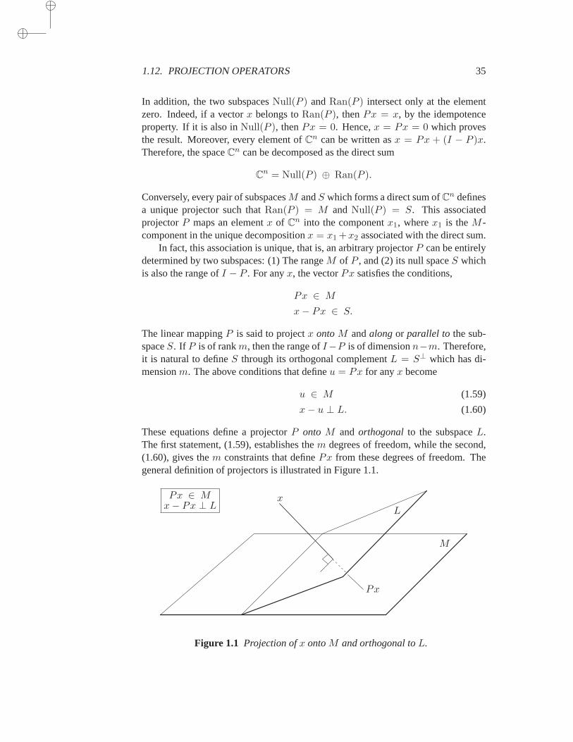
1.12. PROJECTION OPERATORS 35
In addition, the two subspacesNull(P ) andRan(P ) intersect only at the elementzero. Indeed, if a vectorx belongs toRan(P ), thenPx = x, by the idempotenceproperty. If it is also inNull(P ), thenPx = 0. Hence,x = Px = 0 which provesthe result. Moreover, every element ofC
n can be written asx = Px + (I − P )x.Therefore, the spaceCn can be decomposed as the direct sum
Cn = Null(P ) ⊕ Ran(P ).
Conversely, every pair of subspacesM andS which forms a direct sum ofCn definesa unique projector such thatRan(P ) = M and Null(P ) = S. This associatedprojectorP maps an elementx of C
n into the componentx1, wherex1 is theM -component in the unique decompositionx = x1 +x2 associated with the direct sum.
In fact, this association is unique, that is, an arbitrary projectorP can be entirelydetermined by two subspaces: (1) The rangeM of P , and (2) its null spaceS whichis also the range ofI − P . For anyx, the vectorPx satisfies the conditions,
Px ∈ M
x− Px ∈ S.
The linear mappingP is said to projectx ontoM andalongor parallel to the sub-spaceS. If P is of rankm, then the range ofI−P is of dimensionn−m. Therefore,it is natural to defineS through its orthogonal complementL = S⊥ which has di-mensionm. The above conditions that defineu = Px for anyx become
u ∈ M (1.59)
x− u ⊥ L. (1.60)
These equations define a projectorP ontoM and orthogonal to the subspaceL.The first statement, (1.59), establishes them degrees of freedom, while the second,(1.60), gives them constraints that definePx from these degrees of freedom. Thegeneral definition of projectors is illustrated in Figure 1.1.
M
Lx
Px
Px ∈ Mx− Px ⊥ L
Figure 1.1 Projection ofx ontoM and orthogonal toL.
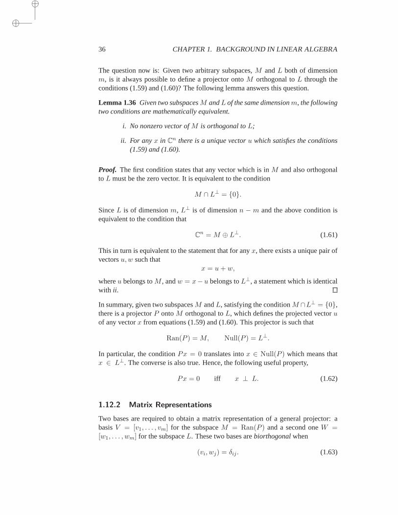
36 CHAPTER 1. BACKGROUND IN LINEAR ALGEBRA
The question now is: Given two arbitrary subspaces,M andL both of dimensionm, is it always possible to define a projector ontoM orthogonal toL through theconditions (1.59) and (1.60)? The following lemma answers this question.
Lemma 1.36 Given two subspacesM andL of the same dimensionm, the followingtwo conditions are mathematically equivalent.
i. No nonzero vector ofM is orthogonal toL;
ii. For any x in Cn there is a unique vectoru which satisfies the conditions
(1.59) and (1.60).
Proof. The first condition states that any vector which is inM and also orthogonaltoL must be the zero vector. It is equivalent to the condition
M ∩ L⊥ = 0.
SinceL is of dimensionm, L⊥ is of dimensionn − m and the above condition isequivalent to the condition that
Cn = M ⊕ L⊥. (1.61)
This in turn is equivalent to the statement that for anyx, there exists a unique pair ofvectorsu,w such that
x = u+ w,
whereu belongs toM , andw = x− u belongs toL⊥, a statement which is identicalwith ii .
In summary, given two subspacesM andL, satisfying the conditionM ∩L⊥ = 0,there is a projectorP ontoM orthogonal toL, which defines the projected vectoruof any vectorx from equations (1.59) and (1.60). This projector is such that
Ran(P ) = M, Null(P ) = L⊥.
In particular, the conditionPx = 0 translates intox ∈ Null(P ) which means thatx ∈ L⊥. The converse is also true. Hence, the following useful property,
Px = 0 iff x ⊥ L. (1.62)
1.12.2 Matrix Representations
Two bases are required to obtain a matrix representation of a general projector: abasisV = [v1, . . . , vm] for the subspaceM = Ran(P ) and a second oneW =[w1, . . . , wm] for the subspaceL. These two bases arebiorthogonalwhen
(vi, wj) = δij . (1.63)
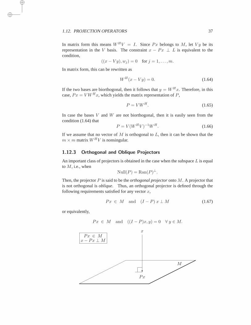
1.12. PROJECTION OPERATORS 37
In matrix form this meansWHV = I. SincePx belongs toM , let V y be itsrepresentation in theV basis. The constraintx − Px ⊥ L is equivalent to thecondition,
((x− V y), wj) = 0 for j = 1, . . . ,m.
In matrix form, this can be rewritten as
WH(x− V y) = 0. (1.64)
If the two bases are biorthogonal, then it follows thaty = WHx. Therefore, in thiscase,Px = VWHx, which yields the matrix representation ofP ,
P = VWH . (1.65)
In case the basesV andW are not biorthogonal, then it is easily seen from thecondition (1.64) that
P = V (WHV )−1WH . (1.66)
If we assume that no vector ofM is orthogonal toL, then it can be shown that them×m matrixWHV is nonsingular.
1.12.3 Orthogonal and Oblique Projectors
An important class of projectors is obtained in the case when the subspaceL is equaltoM , i.e., when
Null(P ) = Ran(P )⊥.
Then, the projectorP is said to be theorthogonal projectorontoM . A projector thatis not orthogonal isoblique. Thus, an orthogonal projector is defined through thefollowing requirements satisfied for any vectorx,
Px ∈ M and (I − P ) x ⊥M (1.67)
or equivalently,
Px ∈ M and ((I − P )x, y) = 0 ∀ y ∈M.
?
Px
x
M
Px ∈ Mx− Px ⊥M
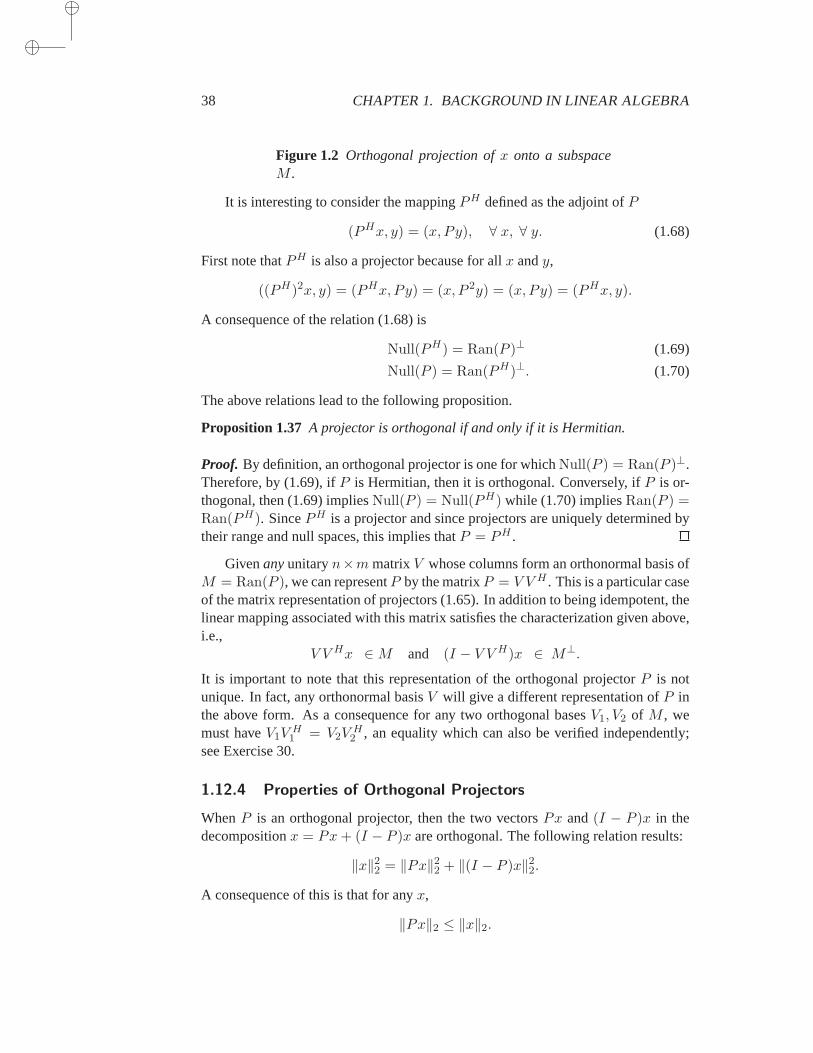
38 CHAPTER 1. BACKGROUND IN LINEAR ALGEBRA
Figure 1.2 Orthogonal projection ofx onto a subspaceM .
It is interesting to consider the mappingPH defined as the adjoint ofP
(PHx, y) = (x, Py), ∀ x, ∀ y. (1.68)
First note thatPH is also a projector because for allx andy,
((PH)2x, y) = (PHx, Py) = (x, P 2y) = (x, Py) = (PHx, y).
A consequence of the relation (1.68) is
Null(PH) = Ran(P )⊥ (1.69)
Null(P ) = Ran(PH)⊥. (1.70)
The above relations lead to the following proposition.
Proposition 1.37 A projector is orthogonal if and only if it is Hermitian.
Proof. By definition, an orthogonal projector is one for whichNull(P ) = Ran(P )⊥.Therefore, by (1.69), ifP is Hermitian, then it is orthogonal. Conversely, ifP is or-thogonal, then (1.69) impliesNull(P ) = Null(PH) while (1.70) impliesRan(P ) =Ran(PH). SincePH is a projector and since projectors are uniquely determined bytheir range and null spaces, this implies thatP = PH .
Givenanyunitaryn×mmatrixV whose columns form an orthonormal basis ofM = Ran(P ), we can representP by the matrixP = V V H . This is a particular caseof the matrix representation of projectors (1.65). In addition to being idempotent, thelinear mapping associated with this matrix satisfies the characterization given above,i.e.,
V V Hx ∈M and (I − V V H)x ∈ M⊥.
It is important to note that this representation of the orthogonal projectorP is notunique. In fact, any orthonormal basisV will give a different representation ofP inthe above form. As a consequence for any two orthogonal basesV1, V2 of M , wemust haveV1V
H1 = V2V
H2 , an equality which can also be verified independently;
see Exercise 30.
1.12.4 Properties of Orthogonal Projectors
WhenP is an orthogonal projector, then the two vectorsPx and(I − P )x in thedecompositionx = Px+ (I − P )x are orthogonal. The following relation results:
‖x‖22 = ‖Px‖22 + ‖(I − P )x‖22.
A consequence of this is that for anyx,
‖Px‖2 ≤ ‖x‖2.
1.13. BASIC CONCEPTS IN LINEAR SYSTEMS 39
Thus, the maximum of‖Px‖2/‖x‖2, for all x in Cn does not exceed one. In addition
the value one is reached for any element inRan(P ). Therefore,
‖P‖2 = 1
for any orthogonal projectorP .An orthogonal projector has only two eigenvalues: zero or one. Any vector of
the range ofP is an eigenvector associated with the eigenvalue one. Any vector ofthe null-space is obviously an eigenvector associated with the eigenvalue zero.
Next, an important optimality property of orthogonal projectors is established.
Theorem 1.38 LetP be the orthogonal projector onto a subspaceM . Then for anygiven vectorx in C
n, the following is true:
miny∈M‖x− y‖2 = ‖x− Px‖2. (1.71)
Proof. Let y be any vector ofM and consider the square of its distance fromx. Sincex− Px is orthogonal toM to whichPx− y belongs, then
‖x− y‖22 = ‖x− Px+ (Px− y)‖22 = ‖x− Px‖22 + ‖(Px− y)‖22.
Therefore,‖x − y‖2 ≥ ‖x − Px‖2 for all y in M . This establishes the result bynoticing that the minimum is reached fory = Px.
By expressing the conditions that definey∗ ≡ Px for an orthogonal projectorPonto a subspaceM , it is possible to reformulate the above result in the form of nec-essary and sufficient conditions which enable us to determine the best approximationto a given vectorx in the least-squares sense.
Corollary 1.39 Let a subspaceM , and a vectorx in Cn be given. Then
miny∈M‖x− y‖2 = ‖x− y∗‖2, (1.72)
if and only if the following two conditions are satisfied,y∗ ∈ Mx− y∗ ⊥ M.
1.13 Basic Concepts in Linear Systems
Linear systems are among the most important and common problems encounteredinscientific computing. From the theoretical point of view, it is well understoodwhena solution exists, when it does not, and when there are infinitely many solutions. Inaddition, explicit expressions of the solution using determinants exist. However, thenumerical viewpoint is far more complex. Approximations may be available but itmay be difficult to estimate how accurate they are. This clearly will depend on thedata at hand, i.e., primarily on the coefficient matrix. This section gives a very briefoverview of the existence theory as well as the sensitivity of the solutions.

40 CHAPTER 1. BACKGROUND IN LINEAR ALGEBRA
1.13.1 Existence of a Solution
Consider thelinear systemAx = b. (1.73)
Here,x is termed theunknownandb the right-hand side.When solving the linearsystem (1.73), we distinguish three situations.
Case 1 The matrixA is nonsingular. There is a unique solution given byx = A−1b.
Case 2 The matrixA is singular andb ∈ Ran(A). Sinceb ∈ Ran(A), there is anx0 such thatAx0 = b. Thenx0 + v is also a solution for anyv in Null(A). SinceNull(A) is at least one-dimensional, there are infinitely many solutions.
Case 3 The matrixA is singular andb /∈ Ran(A). There are no solutions.
Example 1.4. The simplest illustration of the above three cases is with small di-agonal matrices. Let
A =
(2 00 4
)
b =
(18
)
.
ThenA is nonsingular and there is a uniquex given by
x =
(0.52
)
.
Now let
A =
(2 00 0
)
, b =
(10
)
.
ThenA is singular and, as is easily seen,b ∈ Ran(A). For example, a particularelementx0 such thatAx0 = b is x0 =
(0.50
). The null space ofA consists of all
vectors whose first component is zero, i.e., all vectors of the form(
0α
). Therefore,
there are infinitely many solution which are given by
x(α) =
(0.5α
)
∀ α.
Finally, letA be the same as in the previous case, but define the right-hand side as
b =
(11
)
.
In this case there are no solutions because the second equation cannot be satisfied.
1.13. BASIC CONCEPTS IN LINEAR SYSTEMS 41
1.13.2 Perturbation Analysis
Consider the linear system (1.73) whereA is ann × n nonsingular matrix. Givenany matrixE, the matrixA(ǫ) = A+ ǫE is nonsingular forǫ small enough, i.e., forǫ ≤ α whereα is some small number; see Exercise 37. Assume that we perturb thedata in the above system, i.e., that we perturb the matrixA by ǫE and the right-handsideb by ǫe. The solutionx(ǫ) of the perturbed system satisfies the equation,
(A+ ǫE)x(ǫ) = b+ ǫe. (1.74)
Let δ(ǫ) = x(ǫ)− x. Then,
(A+ ǫE)δ(ǫ) = (b+ ǫe)− (A+ ǫE)x
= ǫ (e− Ex)δ(ǫ) = ǫ (A+ ǫE)−1(e− Ex).
As an immediate result, the functionx(ǫ) is differentiable atǫ = 0 and its derivativeis given by
x′(0) = limǫ→0
δ(ǫ)
ǫ= A−1 (e− Ex) . (1.75)
The size of the derivative ofx(ǫ) is an indication of the size of the variation thatthe solutionx(ǫ) undergoes when the data, i.e., the pair[A, b] is perturbed in thedirection[E, e]. In absolute terms, a small variation[ǫE, ǫe] will cause the solutionto vary by roughlyǫx′(0) = ǫA−1(e− Ex). The relative variation is such that
‖x(ǫ)− x‖‖x‖ ≤ ǫ‖A−1‖
( ‖e‖‖x‖ + ‖E‖
)
+ o(ǫ).
Using the fact that‖b‖ ≤ ‖A‖‖x‖ in the above equation yields
‖x(ǫ)− x‖‖x‖ ≤ ǫ‖A‖‖A−1‖
(‖e‖‖b‖ +
‖E‖‖A‖
)
+ o(ǫ) (1.76)
which relates the relative variation in the solution to the relative sizes of the pertur-bations. The quantity
κ(A) = ‖A‖ ‖A−1‖is called thecondition numberof the linear system (1.73) with respect to the norm‖.‖. The condition number is relative to a norm. When using the standard norms‖.‖p,p = 1, . . . ,∞, it is customary to labelκ(A) with the same label as the associatednorm. Thus,
κp(A) = ‖A‖p‖A−1‖p.For large matrices, the determinant of a matrix is almost never a good indication
of “near” singularity or degree of sensitivity of the linear system. The reason is thatdet(A) is the product of the eigenvalues which depends very much on a scaling ofamatrix, whereas the condition number of a matrix is scaling-invariant. For example,
42 CHAPTER 1. BACKGROUND IN LINEAR ALGEBRA
for A = αI the determinant isdet(A) = αn, which can be very small if|α| < 1,whereasκ(A) = 1 for any of the standard norms.
In addition, small eigenvalues do not always give a good indication of poor con-ditioning. Indeed, a matrix can have all its eigenvalues equal to one yet be poorlyconditioned.
Example 1.5. The simplest example is provided by matrices of the form
An = I + αe1eTn
for largeα. The inverse ofAn is
A−1n = I − αe1eTn
and for the∞-norm we have
‖An‖∞ = ‖A−1n ‖∞ = 1 + |α|
so thatκ∞(An) = (1 + |α|)2.
For a largeα, this can give a very large condition number, whereas all the eigenvaluesof An are equal to unity.
When an iterative procedure is used for solving a linear system, we typicallyface the problem of choosing a good stopping procedure for the algorithm. Often aresidual norm,
‖r‖ = ‖b−Ax‖is available for some current approximationx and an estimate of the absolute error‖x− x‖ or the relative error‖x− x‖/‖x‖ is desired. The following simple relationis helpful in this regard,
‖x− x‖‖x‖ ≤ κ(A)
‖r‖‖b‖ .
It is necessary to have an estimate of the condition numberκ(A) in order to exploitthe above relation.
PROBLEMS
P-1.1 Verify that the Euclidean inner product defined by (1.4) doesindeed satisfy the gen-eral definition of inner products on vector spaces.
P-1.2 Show that two eigenvectors associated with two distinct eigenvalues are linearly inde-pendent. In a more general sense, show that a family of eigenvectors associated with distincteigenvalues forms a linearly independent family.
1.13. BASIC CONCEPTS IN LINEAR SYSTEMS 43
P-1.3 Show that ifλ is any nonzero eigenvalue of the matrixAB, then it is also an eigen-value of the matrixBA. Start with the particular case whereA andB are square andBis nonsingular, then consider the more general case whereA,B may be singular or evenrectangular (but such thatAB andBA are square).
P-1.4 LetA be ann×n orthogonal matrix, i.e., such thatAHA = D, whereD is a diagonalmatrix. Assuming thatD is nonsingular, what is the inverse ofA? Assuming thatD > 0,how canA be transformed into a unitary matrix (by operations on its rows or columns)?
P-1.5 Show that the Frobenius norm is consistent. Can this norm be associated to two vectornorms via (1.7)? What is the Frobenius norm of a diagonal matrix? What is thep-norm of adiagonal matrix (for anyp)?
P-1.6 Find the Jordan canonical form of the matrix:
A =
1 2 −40 1 20 0 2
.
Same question for the matrix obtained by replacing the element a33 by 1.
P-1.7 Give an alternative proof of Theorem 1.9 on the Schur form by starting from theJordan canonical form. [Hint: WriteA = XJX−1 and use the QR decomposition ofX.]
P-1.8 Show from the definition of determinants used in Section 1.2 that the characteristicpolynomial is a polynomial of degreen for ann× n matrix.
P-1.9 Show that the characteristic polynomials of two similar matrices are equal.
P-1.10 Show thatlim
k→∞‖Ak‖1/k = ρ(A),
for any matrix norm. [Hint: Use the Jordan canonical form.]
P-1.11 LetX be a nonsingular matrix and, for any matrix norm‖.‖, define‖A‖X = ‖AX‖.Show that this is indeed a matrix norm. Is this matrix norm consistent? Show the same for‖XA‖ and‖Y AX‖ whereY is also a nonsingular matrix. These norms are not, in general,associated with any vector norms, i.e., they can’t be definedby a formula of the form (1.7).Why? What can you say about the particular case whenY = X−1? Is‖X−1AX‖ inducedby a vector norm in this particular case?
P-1.12 Find the field of values of the matrix
A =
(0 10 0
)
and verify that it is not equal to the convex hull of its eigenvalues.
P-1.13 Show that for a skew-Hermitian matrixS,
ℜe(Sx, x) = 0 for anyx ∈ Cn.
P-1.14 Given an arbitrary matrixS, show that if(Sx, x) = 0 for all x in Cn, then it is true
that(Sy, z) + (Sz, y) = 0 ∀ y, z ∈ C
n. (1.77)
[Hint: Expand(S(y + z), y + z).]
44 CHAPTER 1. BACKGROUND IN LINEAR ALGEBRA
P-1.15 Using the results of the previous two problems, show that if(Ax, x) is real for allx in C
n, thenA must be Hermitian. Would this result be true if the assumption were to bereplaced by:(Ax, x) is real for all realx? Explain.
P-1.16 Show that if(Sx, x) = 0 for all complex vectorsx, thenS is zero. [Hint: Start bydoing Problem 14. Then selectingy = ek, z = eθej in (1.77), for an arbitraryθ, establishthatskje
2θ = −sjk and conclude thatsjk = sjk = 0]. Is the result true if(Sx, x) = 0 forall real vectorsx?
P-1.17 The definition of a positive definite matrix is that(Ax, x) be real and positive for allreal vectorsx. Show that this is equivalent to requiring that the Hermitian part ofA, namely,12 (A+AH), be (Hermitian) positive definite.
P-1.18 LetA1 = B−1C andA2 = CB whereC is a Hermitian matrix andB is a HermitianPositive Definite matrix. AreA1 andA2 Hermitian in general? Show thatA1 andA2 areHermitian (self-adjoint) with respect to theB-inner product.
P-1.19 Let a matrixA be such thatAH = p(A) wherep is a polynomial. Show thatA isnormal. Given a diagonal complex matrixD, show that there exists a polynomial of degree< n such thatD = p(D). Use this to show that a normal matrix satisfiesAH = p(A) fora certain polynomial ofp of degree< n. As an application, use this result to provide analternative proof of Lemma 1.13.
P-1.20 Show thatA is normal iff its Hermitian and skew-Hermitian parts, as defined inSection 1.11, commute.
P-1.21 The goal of this exercise is to establish the relation (1.35). Consider the numericalradiusν(A) of an arbitrary matrixA. Show thatν(A) ≤ ‖A‖2. Show that for a normalmatrix ν(A) = ‖A‖2. Consider the decomposition of a matrix into its Hermtian and skew-Hermitian parts as shown in (1.49), (1.50), and (1.51). Showthat‖A‖2 ≤ ν(H)+ν(S). Now,using this inequality and the definition of the numerical radius show that‖A‖2 ≤ 2ν(A).
P-1.22 Show that the numerical radius is a vector norm in the sense that it satisfies the threeproperties (1.8–1.10) of norms. [Hint: For (1.8) solve exercise 16 first]. Find a counter-example to show that the numerical radius is not a (consistent) matrix norm, i.e., thatν(AB)can be larger thanν(A) ν(B).
P-1.23 LetA be a Hermitian matrix andB a Hermitian Positive Definite matrix defining aB-inner product. Show thatA is Hermitian (self-adjoint) with respect to theB-inner productif and only if A andB commute. What condition must satisfyB for the same condition tohold in the more general case whereA is not Hermitian?
P-1.24 Let A be a real symmetric matrix andλ an eigenvalue ofA. Show that ifu is aneigenvector associated withλ, then so isu. As a result, prove that for any eigenvalue of areal symmetric matrix, there is an associated eigenvector which is real.
P-1.25 Show that a Hessenberg matrixH such thathj+1,j 6= 0, j = 1, 2, . . . , n− 1, cannotbe derogatory.
P-1.26 Prove all the properties listed in Proposition 1.24.
P-1.27 Let A be anM -matrix andu, v two nonnegative vectors such thatvTA−1u < 1.Show thatA− uvT is anM -matrix.
P-1.28 Show that ifO ≤ A ≤ B thenO ≤ ATA ≤ BTB. Conclude that under the sameassumption, we have‖A‖2 ≤ ‖B‖2.

1.13. BASIC CONCEPTS IN LINEAR SYSTEMS 45
P-1.29 Consider the subspaceM of R4 spanned by the vectors
v1 =
1011
; v2 =
1−10−1
a. Write down the matrix representing the orthogonal projector ontoM .
b. What is the null space ofP?
c. What is its range?
d. Find the vectorx in S which is the closest in the 2-norm sense to the vectorc =[1, 1, 1, 1]T
P-1.30 Show that for two orthonormal basesV1, V2 of the same subspaceM of Cn we have
V1VH1 x = V2V
H2 x, ∀ x.
P-1.31 What are the eigenvalues of a projector? What about its eigenvectors?
P-1.32 Show that if two projectorsP1 andP2 commute, then their productP = P1P2 is aprojector. What are the range and kernel ofP?
P-1.33 Theorem 1.32 shows that the condition (2) in Definition 1.30 is not needed, i.e., itis implied by (4) (and the other conditions). One is tempted to say that only one of (2) or (4)is required. Is this true? In other words, does (2) also imply(4)? [Prove or show a counterexample]
P-1.34 Consider the matrixA of sizen× n and the vectorx ∈ Rn,
A =
1 −1 −1 −1 . . . −10 1 −1 −1 . . . −10 0 1 −1 . . . −1...
......
. . ....
......
......
. . ....
0 0 0 . . . 0 1
x =
11/21/41/8
...1/2n−1
.
a. ComputeAx, ‖Ax‖2, and‖x‖2.
b. Show that‖A‖2 ≥√n.
c. Give a lower bound forκ2(A).
P-1.35 What is the inverse of the matrixA of the previous exercise? Give an expression ofκ1(A) andκ∞(A) based on this.
P-1.36 Find a small rank-one perturbation which makes the matrixA in Exercise 34 singu-lar. Derive a lower bound for the singular values ofA.
P-1.37 Consider a nonsingular matrixA. Given any matrixE, show that there existsα suchthat the matrixA(ǫ) = A+ǫE is nonsingular for allǫ < α. What is the largest possible valuefor α satisfying the condition? [Hint: Consider the eigenvaluesof the generalized eigenvalueproblemAu = λEu.]
NOTES ANDREFERENCES. For additional reading on the material presented in this chapter, see Goluband Van Loan [149], Meyer [210], Demmel [99], Datta [93], Stewart [273], and Varga [293]. Volume2 (“Eigensystems”) of the series [274], offers an up-to-date coverage of algorithms for eigenvalue

46 CHAPTER 1. BACKGROUND IN LINEAR ALGEBRA
problems. The excellent treatise of nonnegative matrices in the book by Varga [293] remains a goodreference on this topic and on iterative methods four decades after its first publication. State-of-the-artcoverage on iterative methods up to the very beginning of the 1970s can be found in the book by Young[322] which coversM -matrices and related topics in great detail. For a good overview of the linearalgebra aspects of matrix theory and a complete proof of Jordan’s canonical form, Halmos [164] isrecommended.
Chapter 2
DISCRETIZATION OF PDES
Partial Differential Equations (PDEs) constitute by far the biggest source of sparse matrix
problems. The typical way to solve such equations is to discretize them, i.e., to approximate
them by equations that involve a finite number of unknowns. The matrix problems that arise
from these discretizations are generally large and sparse, i.e., they have very few nonzero entries.
There are several different ways to discretize a Partial Differential Equation. The simplest method
uses finite difference approximations for the partial differential operators. The Finite Element
Method replaces the original function by a function which has some degree of smoothness over
the global domain, but which is piecewise polynomial on simple cells, such as small triangles
or rectangles. This method is probably the most general and well understood discretization
technique available. In between these two methods, there are a few conservative schemes called
Finite Volume Methods, which attempt to emulate continuous conservation laws of physics. This
chapter introduces these three different discretization methods.
2.1 Partial Differential Equations
Physical phenomena are often modeled by equations that relate several partial deriva-tives of physical quantities, such as forces, momentums, velocities, energy, tempera-ture, etc. These equations rarely have aclosed-form(explicit) solution. In this chap-ter, a few types of Partial Differential Equations are introduced, which willserve asmodels throughout the book. Only one- or two-dimensional problems are considered,and the space variables are denoted byx in the case of one-dimensional problems orx1 andx2 for two-dimensional problems. In two dimensions,x denotes the “vector”of components(x1, x2).
2.1.1 Elliptic Operators
One of the most common Partial Differential Equations encountered in various areasof engineering is Poisson’s equation:
∂2u
∂x21
+∂2u
∂x22
= f, for x =
(x1
x2
)
in Ω (2.1)
whereΩ is a bounded, open domain inR2. Here,x1, x2 are the two space variables.
47

48 CHAPTER 2. DISCRETIZATION OF PDES
~n
x1
x2 Ω
Γ
Figure 2.1: DomainΩ for Poisson’s equation.
The above equation is to be satisfied only for points that are located at the interiorof the domainΩ. Equally important are the conditions that must be satisfied on theboundaryΓ of Ω. These are termedboundary conditions, and they come in threecommon types:
Dirichlet condition u(x) = φ(x)
Neumann condition ∂u∂~n(x) = 0
Cauchy condition ∂u∂~n(x) + α(x)u(x) = γ(x)
The vector~n usually refers to a unit vector that is normal toΓ and directedoutwards. Note that the Neumann boundary conditions are a particular case of theCauchy conditions withγ = α = 0. For a given unit vector,~v with componentsv1andv2, the directional derivative∂u/∂~v is defined by
∂u
∂~v(x) = lim
h→0
u(x+ h~v)− u(x)h
=∂u
∂x1(x)v1 +
∂u
∂x2(x)v2 (2.2)
= ∇u.~v (2.3)
where∇u is the gradient ofu,
∇u =
(∂u∂x1
∂u∂x2
)
, (2.4)
and the dot in (2.3) indicates a dot product of two vectors inR2.
In reality, Poisson’s equation is often a limit case of a time-dependent problem.Its solution can, for example, represent the steady-state temperature distribution ina regionΩ when there is a heat sourcef that is constant with respect to time. Theboundary conditions should then model heat loss across the boundaryΓ.
The particular case wheref(x) = 0, i.e., the equation
∆u = 0,
2.1. PARTIAL DIFFERENTIAL EQUATIONS 49
to which boundary conditions must be added, is called theLaplace equationand itssolutions are calledharmonic functions.
Many problems in physics have boundary conditions ofmixed type, e.g., ofDirichlet type in one part of the boundary and of Cauchy type in another.Another ob-servation is that the Neumann conditions do not define the solution uniquely. Indeed,if u is a solution, then so isu+ c for any constantc.
The operator
∆ =∂2
∂x21
+∂2
∂x22
is called theLaplacean operatorand appears in many models of physical and me-chanical phenomena. These models often lead to more general elliptic operators ofthe form
L =∂
∂x1
(
a∂
∂x1
)
+∂
∂x2
(
a∂
∂x2
)
= ∇. (a∇) (2.5)
where the scalar functiona depends on the coordinate and may represent some spe-cific parameter of the medium, such as density, porosity, etc. At this point it maybe useful to recall some notation which is widely used in physics and mechanics.The∇ operator can be considered as a vector consisting of the components∂
∂x1and
∂∂x2
. When applied to a scalar functionu, this operator is nothing but thegradientoperator, since it yields a vector with the components∂u
∂x1and ∂u
∂x2as is shown in
(2.4). The dot notation allows dot products of vectors inR2 to be defined. These
vectors can include partial differential operators. For example, the dotproduct∇.uof∇ with u =
(u1
u2
)
yields the scalar quantity,
∂u1
∂x1+∂u2
∂x2,
which is called thedivergenceof the vector function~u =(
u1
u2
)
. Applying thisdivergence operatorto u = a∇, wherea is a scalar function, yields theL operatorin (2.5). The divergence of the vector function~v is often denoted by div~v or∇.~v.Thus,
div ~v = ∇.~v =∂v1∂x1
+∂v2∂x2
.
The closely related operator
L =∂
∂x1
(
a1∂
∂x1
)
+∂
∂x2
(
a2∂
∂x2
)
= ∇ (~a.∇) (2.6)
is a further generalization of the Laplacean operator∆ in the case where the mediumis anisotropicandinhomogeneous.The coefficientsa1, a2 depend on the space vari-ablex and reflect the position as well as the directional dependence of the materialproperties, such as porosity in the case of fluid flow or dielectric constantsin electro-statics. In fact, the above operator can be viewed as a particular case ofL = ∇.(A∇),whereA is a2× 2 matrix which acts on the two components of∇.

50 CHAPTER 2. DISCRETIZATION OF PDES
2.1.2 The Convection Diffusion Equation
Many physical problems involve a combination of “diffusion” and “convection” phe-nomena. Such phenomena are modeled by the convection-diffusion equation
∂u
∂t+ b1
∂u
∂x1+ b2
∂u
∂x2= ∇.(a∇)u+ f
or∂u
∂t+~b.∇u = ∇.(a∇)u+ f
the steady-state version of which can be written as
−∇.(a∇)u+~b.∇u = f. (2.7)
Problems of this type are often used as model problems because they represent thesimplest form of conservation of mass in fluid mechanics. Note that the vector~b issometimes quite large, which may cause some difficulties either to the discretizationschemes or to the iterative solution techniques.
2.2 Finite Difference Methods
Thefinite differencemethod is based on local approximations of the partial deriva-tives in a Partial Differential Equation, which are derived by low order Taylor seriesexpansions. The method is quite simple to define and rather easy to implement.Also, it is particularly appealing for simple regions, such as rectangles, and whenuniform meshes are used. The matrices that result from these discretizations areoften well structured, which means that they typically consist of a few nonzero di-agonals. Another advantage is that there are a number of “fast Poissonsolvers” forconstant coefficient problems, which can deliver the solution in logarithmic timepergrid point. This means the total number of operations is of the order ofn log(n)wheren is the total number of discretization points. This section gives an overviewof finite difference discretization techniques.
2.2.1 Basic Approximations
The simplest way to approximate the first derivative of a functionu at the pointx isvia the formula (
du
dx
)
(x) ≈ u(x+ h)− u(x)h
. (2.8)
Whenu is differentiable atx, then the limit of the above ratio whenh tends to zero isthe derivative ofu atx. For a function that isC4 in the neighborhood ofx, we haveby Taylor’s formula
u(x+ h) = u(x) + hdu
dx+h2
2
d2u
dx2+h3
6
d3u
dx3+h4
24
d4u
dx4(ξ+), (2.9)

2.2. FINITE DIFFERENCE METHODS 51
for someξ+ in the interval(x, x + h). Therefore, the above approximation (2.8)satisfies
du
dx=u(x+ h)− u(x)
h− h
2
d2u(x)
dx2+O(h2). (2.10)
The formula (2.9) can be rewritten withh replaced by−h to obtain
u(x− h) = u(x)− hdudx
+h2
2
d2u
dx2− h3
6
d3u
dx3+h4
24
d4u(ξ−)
dx4, (2.11)
in which ξ− belongs to the interval(x − h, x). Adding (2.9) and (2.11), dividingthrough byh2, and using the mean value theorem for the fourth order derivativesresults in the following approximation of the second derivative
d2u(x)
dx2=
u(x+ h)− 2u(x) + u(x− h)h2
− h2
12
d4u(ξ)
dx4, (2.12)
whereξ− ≤ ξ ≤ ξ+. The above formula is called acentered difference approxima-tion of the second derivative since the point at which the derivative is beingapprox-imated is the center of the points used for the approximation. The dependenceofthis derivative on the values ofu at the points involved in the approximation is oftenrepresented by a “stencil” or “molecule,” shown in Figure 2.2.
1 −2 1
Figure 2.2: The three-point stencil for the centered difference approximation to thesecond order derivative.
The approximation (2.8) for the first derivative isforward rather than centered.Also, abackwardformula can be used which consists of replacinghwith−h in (2.8).The two formulas can also be averaged to obtain thecentered differenceformula:
du(x)
dx≈ u(x+ h)− u(x− h)
2 h. (2.13)
It is easy to show that the above centered difference formula is of the secondorder, while (2.8) is only first order accurate. Denoted byδ+ andδ−, the forwardand backward difference operators are defined by
δ+u(x) = u(x+ h)− u(x) (2.14)
δ−u(x) = u(x)− u(x− h). (2.15)
All previous approximations can be rewritten using these operators.In addition to standard first order and second order derivatives, it issometimes
necessary to approximate the second order operator
d
dx
[
a(x)d
dx
]
.
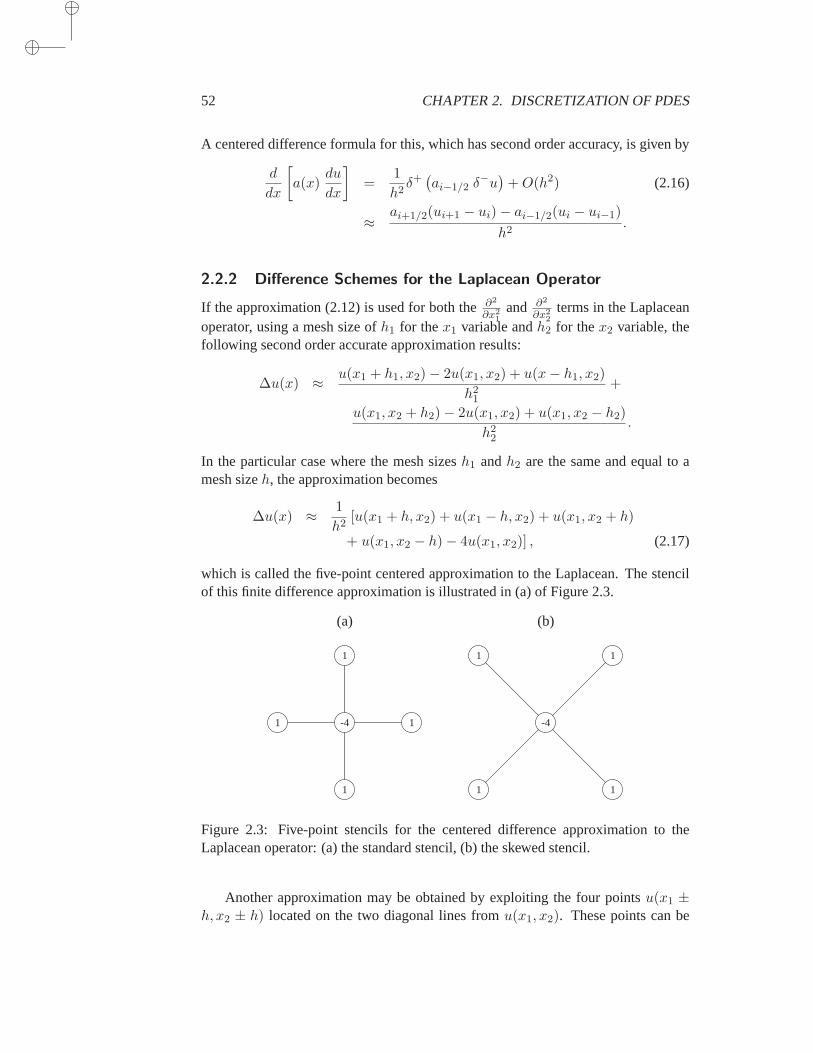
52 CHAPTER 2. DISCRETIZATION OF PDES
A centered difference formula for this, which has second order accuracy, is given by
d
dx
[
a(x)du
dx
]
=1
h2δ+(ai−1/2 δ
−u)
+O(h2) (2.16)
≈ai+1/2(ui+1 − ui)− ai−1/2(ui − ui−1)
h2.
2.2.2 Difference Schemes for the Laplacean Operator
If the approximation (2.12) is used for both the∂2
∂x21
and ∂2
∂x22
terms in the Laplaceanoperator, using a mesh size ofh1 for thex1 variable andh2 for thex2 variable, thefollowing second order accurate approximation results:
∆u(x) ≈ u(x1 + h1, x2)− 2u(x1, x2) + u(x− h1, x2)
h21
+
u(x1, x2 + h2)− 2u(x1, x2) + u(x1, x2 − h2)
h22
.
In the particular case where the mesh sizesh1 andh2 are the same and equal to amesh sizeh, the approximation becomes
∆u(x) ≈ 1
h2[u(x1 + h, x2) + u(x1 − h, x2) + u(x1, x2 + h)
+ u(x1, x2 − h)− 4u(x1, x2)] , (2.17)
which is called the five-point centered approximation to the Laplacean. The stencilof this finite difference approximation is illustrated in (a) of Figure 2.3.
(a)
1
1 -4 1
1
(b)
1 1
-4
1 1
Figure 2.3: Five-point stencils for the centered difference approximation to theLaplacean operator: (a) the standard stencil, (b) the skewed stencil.
Another approximation may be obtained by exploiting the four pointsu(x1 ±h, x2 ± h) located on the two diagonal lines fromu(x1, x2). These points can be
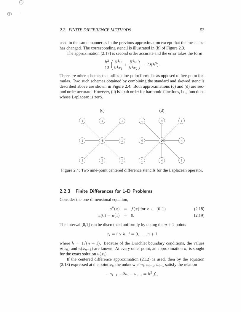
2.2. FINITE DIFFERENCE METHODS 53
used in the same manner as in the previous approximation except that the mesh sizehas changed. The corresponding stencil is illustrated in (b) of Figure 2.3.
The approximation (2.17) is second order accurate and the error takes the form
h2
12
(∂4u
∂4x1+
∂4u
∂4x2
)
+O(h3).
There are other schemes that utilize nine-point formulas as opposed to five-point for-mulas. Two such schemes obtained by combining the standard and skewed stencilsdescribed above are shown in Figure 2.4. Both approximations (c) and (d) are sec-ond order accurate. However, (d) is sixth order for harmonic functions, i.e., functionswhose Laplacean is zero.
(c)
1 1 1
1 -8 1
1 1 1
(d)
1 4 1
4 -20 4
1 4 1
Figure 2.4: Two nine-point centered difference stencils for the Laplacean operator.
2.2.3 Finite Differences for 1-D Problems
Consider the one-dimensional equation,
− u′′(x) = f(x) for x ∈ (0, 1) (2.18)
u(0) = u(1) = 0. (2.19)
The interval [0,1] can be discretized uniformly by taking then+ 2 points
xi = i× h, i = 0, . . . , n+ 1
whereh = 1/(n + 1). Because of the Dirichlet boundary conditions, the valuesu(x0) andu(xn+1) are known. At every other point, an approximationui is soughtfor the exact solutionu(xi).
If the centered difference approximation (2.12) is used, then by the equation(2.18) expressed at the pointxi, the unknownsui, ui−1, ui+1 satisfy the relation
−ui−1 + 2ui − ui+1 = h2 fi,
54 CHAPTER 2. DISCRETIZATION OF PDES
in which fi ≡ f(xi). Notice that fori = 1 and i = n, the equation will involveu0 andun+1 which are known quantities, both equal to zero in this case. Thus, forn = 6, the linear system obtained is of the form
Ax = f
where
A =1
h2
2 −1−1 2 −1
−1 2 −1−1 2 −1
−1 2 −1−1 2
.
2.2.4 Upwind Schemes
Consider now the one-dimensional version of the convection-diffusion equation (2.7)in which the coefficientsa andb are constant, andf = 0, using Dirichlet boundaryconditions,
−a u′′ + b u′ = 0, 0 < x < L = 1u(0) = 0, u(L) = 1.
(2.20)
In this particular case, it is easy to verify that the exact solution to the aboveequationis given by
u(x) =1− eRx
1− eRwhereR is the so-called Peclet number defined byR = bL/a. Now consider theapproximate solution provided by using the centered difference schemes seen above,for both the first- and second order derivatives. The equation for unknown numberibecomes
bui+1 − ui−1
2h− aui+1 − 2ui + ui−1
h2= 0,
or, definingc = Rh/2,
− (1− c)ui+1 + 2ui − (1 + c)ui−1 = 0. (2.21)
This is a second order homogeneous linear difference equation and the usual way tosolve it is to seek a general solution in the formuj = rj . Substituting in (2.21),rmust satisfy
(1− c)r2 − 2r + (c+ 1) = 0.
Therefore,r1 = 1 is a root and the second root isr2 = (1 + c)/(1− c). The generalsolution of the above difference equation is now sought as a linear combination ofthe two solutions corresponding to these two roots,
ui = αri1 + βri
2 = α+ β
(1 + c
1− c
)i
.
2.2. FINITE DIFFERENCE METHODS 55
Because of the boundary conditionu0 = 0, it is necessary thatβ = −α. Likewise,the boundary conditionun+1 = 1 yields
α =1
1− σn+1with σ ≡ 1 + c
1− c .
Thus, the solution is
ui =1− σi
1− σn+1.
Whenh > 2/R the factorσ becomes negative and the above approximations willoscillate around zero. In contrast, the exact solution is positive and monotone inthe range[0, 1]. In this situation the solution is very inaccurate regardless of thearithmetic. In other words, the scheme itself creates the oscillations. To avoid this, asmall enough meshh can be taken to ensure thatc < 1. The resulting approximationis in much better agreement with the exact solution. Unfortunately, this conditioncan limit the mesh size too drastically for large values ofb.
Note that whenb < 0, the oscillations disappear sinceσ < 1. In fact, a linearalgebra interpretation of the oscillations comes from comparing the tridiagonalma-trices obtained from the discretization. Again, for the casen = 6, the tridiagonalmatrix resulting from discretizing the equation (2.7) takes the form
A =1
h2
2 −1 + c−1− c 2 −1 + c
−1− c 2 −1 + c−1− c 2 −1 + c
−1− c 2 −1 + c−1− c 2
.
The above matrix is no longer a diagonally dominant M-matrix. Observe that if thebackward difference formula for the first order derivative is used,we obtain
bui − ui−1
h− aui−1 − 2ui + ui+1
h2= 0.
Then (weak) diagonal dominance is preserved ifb > 0. This is because the newmatrix obtained for the above backward scheme is
A =1
h2
2 + c −1−1− c 2 + c −1
−1− c 2 + c −1−1− c 2 + c −1
−1− c 2 + c −1−1− c 2 + c
wherec is now defined byc = Rh. Each diagonal termaii gets reinforced by thepositive termc while each subdiagonal termai,i−1 increases by the same amount inabsolute value. In the case whereb < 0, the forward difference formula
bui+1 − ui
h− aui−1 − 2ui + ui+1
h2= 0
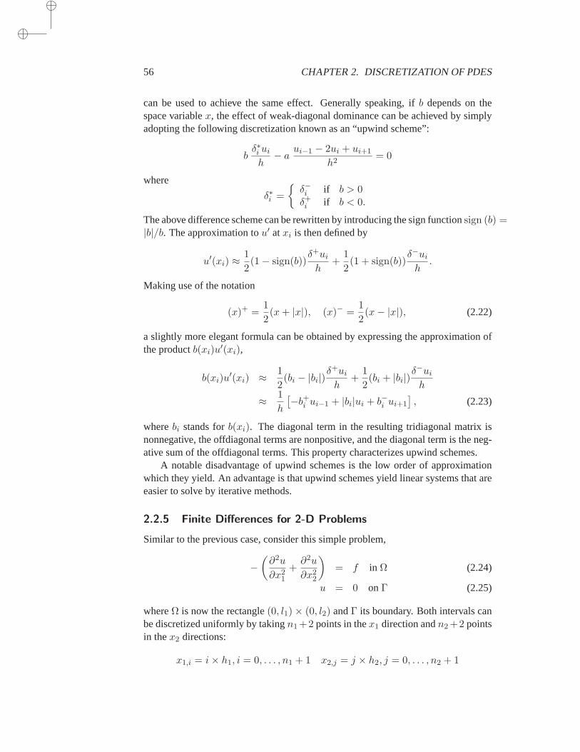
56 CHAPTER 2. DISCRETIZATION OF PDES
can be used to achieve the same effect. Generally speaking, ifb depends on thespace variablex, the effect of weak-diagonal dominance can be achieved by simplyadopting the following discretization known as an “upwind scheme”:
bδ∗i ui
h− a ui−1 − 2ui + ui+1
h2= 0
where
δ∗i =
δ−i if b > 0δ+i if b < 0.
The above difference scheme can be rewritten by introducing the sign functionsign (b) =|b|/b. The approximation tou′ atxi is then defined by
u′(xi) ≈1
2(1− sign(b))
δ+ui
h+
1
2(1 + sign(b))
δ−ui
h.
Making use of the notation
(x)+ =1
2(x+ |x|), (x)− =
1
2(x− |x|), (2.22)
a slightly more elegant formula can be obtained by expressing the approximation ofthe productb(xi)u
′(xi),
b(xi)u′(xi) ≈
1
2(bi − |bi|)
δ+ui
h+
1
2(bi + |bi|)
δ−ui
h
≈ 1
h
[−b+i ui−1 + |bi|ui + b−i ui+1
], (2.23)
wherebi stands forb(xi). The diagonal term in the resulting tridiagonal matrix isnonnegative, the offdiagonal terms are nonpositive, and the diagonalterm is the neg-ative sum of the offdiagonal terms. This property characterizes upwindschemes.
A notable disadvantage of upwind schemes is the low order of approximationwhich they yield. An advantage is that upwind schemes yield linear systems thatareeasier to solve by iterative methods.
2.2.5 Finite Differences for 2-D Problems
Similar to the previous case, consider this simple problem,
−(∂2u
∂x21
+∂2u
∂x22
)
= f in Ω (2.24)
u = 0 onΓ (2.25)
whereΩ is now the rectangle(0, l1)× (0, l2) andΓ its boundary. Both intervals canbe discretized uniformly by takingn1 +2 points in thex1 direction andn2 +2 pointsin thex2 directions:
x1,i = i× h1, i = 0, . . . , n1 + 1 x2,j = j × h2, j = 0, . . . , n2 + 1
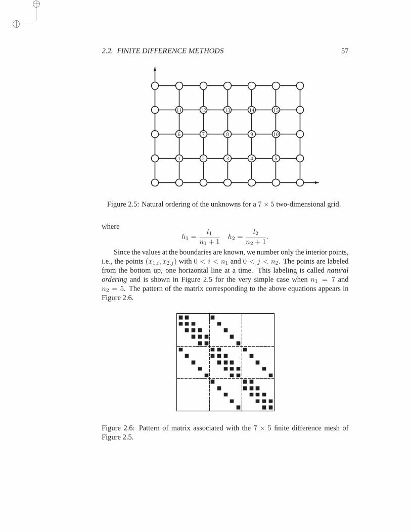
2.2. FINITE DIFFERENCE METHODS 57
1 2 3 4 5
6 7 8 9 10
11 12 13 14 15
-
6
Figure 2.5: Natural ordering of the unknowns for a7× 5 two-dimensional grid.
whereh1 =
l1n1 + 1
h2 =l2
n2 + 1.
Since the values at the boundaries are known, we number only the interior points,i.e., the points(x1,i, x2,j) with 0 < i < n1 and0 < j < n2. The points are labeledfrom the bottom up, one horizontal line at a time. This labeling is callednaturalordering and is shown in Figure 2.5 for the very simple case whenn1 = 7 andn2 = 5. The pattern of the matrix corresponding to the above equations appears inFigure 2.6.
Figure 2.6: Pattern of matrix associated with the7 × 5 finite difference mesh ofFigure 2.5.
58 CHAPTER 2. DISCRETIZATION OF PDES
In the case whenh1 = h2 = h the matrix has the following block structure:
A =1
h2
B −I−I B −I
−I B
with B =
4 −1−1 4 −1
−1 4 −1−1 4
.
2.2.6 Fast Poisson Solvers
A number of special techniques have been developed for solving linear systems aris-ing from finite difference discretizations of the Poisson equation on rectangular grids.These are termed Fast Poisson Solvers (FPS) because of the relativelylow numberof arithmetic operations whuch they require, typically of the order ofO(N log(N))whereN is the size of the matrix.
Consider first the linear systems seen in the previous subsection, which have theform (after scaling byh2)
B −I−I B −I
.. . .. . . . .−I B −I
−I B
u1
u2...
um−1
um
=
b1b2...
bm−1
bm
(2.26)
in which
B =
4 −1−1 4 −1
. .. . .. . ..−1 4 −1
−1 4
(2.27)
The notation has changed slightly in that we callp andm the mesh sizes in thex1
andx2 directions respectively. Therefore, eachui if of dimensionp and correspondsto a block of solution components along one horizontal line.
Fourier methods exploit the knowledge of the eigenvalues and eigenvectors ofthe matrixB. The eigenvalues are known to be
λj = 4− 2 cos
(jπ
p+ 1
)
j = 1, . . . , p
and, definingθj ≡ (jπ)/(p+ 1), the corresponding eigenvectors are given by:
qj =
√2
p+ 1× [sin θj , sin(2θj), . . . , sin(pθj)]
T .
Defining,Q = [q1, . . . , qp]
2.2. FINITE DIFFERENCE METHODS 59
it is clear thatQTBQ = Λ = diag (λj). Thej-th (block)-row of the system (2.26)which can be written as
−uj−1 +Buj − uj+1 = bj ,
will now be transformed by applying the similarity transformationQ to the aboveequation, leading to
−QTuj−1 + (QTBQ) QTuj −QTuj+1 = QT bj
If we denote by a bar quantities expressed in theQ basis, then the above equationbecomes
−uj−1 + Λuj − uj+1 = bj .
Note that the transformation fromuj to uj can be performed with a (real) Fast FourierTransform and this will be exploited shortly. Together the above equationsyield thelarge system,
Λ −I−I Λ −I
.. . .. . . . .−I Λ −I
−I Λ
u1
u2...
um−1
um
=
b1b2...
bm−1
bm
(2.28)
As it turns out, the above system disguises a set ofm independent tridiagonal sys-tems. Indeed, taking thei-th row of each block, yields
λi −1−1 λi −1
. .. . .. .. .−1 λi −1
−1 λi
ui1
ui2...
uip−1
uip
=
bi1bi2...
bip−1
bip
(2.29)
whereuij andbij represent thej-th components of the vectorsuj andbj respectively.The procedure becomes clear and is described in the next algorithm.
ALGORITHM 2.1 FFT-based Fast-Poisson Solver
1. Computebj = QT bj , j = 1, . . . ,m2. Solve the tridiagonal systems (2.29) fori = 1, . . . , p3. Computeuj = Quj , j = 1, . . . ,m
The operations in Lines 1 and 3 are performed by FFT transforms, and require atotal ofO(p log2 p) operations each, leading to a total ofO(m×p log2 p) operations.Solving them tridiagonal systems requires a total of8 × p × m operations. As aresult, the complexity of the algorithm isO(NlogN) whereN = p×m.

60 CHAPTER 2. DISCRETIZATION OF PDES
A second class of Fast Poisson Solvers utilize Block Cyclic Reduction (BCR).For simplicity, assume thatp = 2µ − 1. Denoting2r by h, at ther-th step of BCR,the system is of the following form:
B(r) −I−I B(r) −I
. . . . .. . . .−I B(r) −I
−I B(r)
uh
u2h...
u(pr−1)h
uprh
=
bhb2h...
b(pr−1)h
bprh
(2.30)
Equations whose block-indexj is odd are now eliminated by multiplying each equa-tion indexed2jh byB(r) and adding it to equations(2j − 1)h and(2j + 1)h. Thiswould yield a system with a size half that of (2.30), which involves only the equationswith indices that are even multiples ofh:
−u(2j−2)h +[
(B(r))2 − 2I]
u2jh − u(2j+2)h = B(r)b2jh + b(2j−1)h + b(2j+1)h .
The process can then be repeated until we have only one system ofm equations. Thiscould then be solved and the other unknowns recovered from it in a back-substitution.The method based on this direct approach is not stable.
A stable modification due to Buneman [69] consists of writing the right-handsides differently. Eachbjh is written as
b(r)jh = B(r)p
(r)jh + q
(r)jh (2.31)
Initially, when r = 0, the vectorp(0)i is zero andq(0)i ≡ bj . The elimination of
block-rowjh proceeds in the same manner, as was described above, leading to
− u(2j−2)h +[
(B(r))2 − 2I]
u2jh − u(2j+2)h = (B(r))2p(r)2jh +
B(r)(q(r)2jh + p
(r)(2j−1)h + p
(r)(2j+1)h) + q
(r)(2j−1)h + q
(r)(2j+1)h .(2.32)
It is clear that the diagonal block matrix for the next step is
B(r+1) = (B(r))2 − 2I . (2.33)
It remains to recast Equation (2.32) in a such way that the right-hand side blocks areagain in the form (2.31). The new right-hand side is rewritten as
b(r+1)2jh = (B(r))2
[
p(r)2jh + (B(r))−1(q
(r)2jh + p
(r)(2j−1)h + p
(r)(2j+1)h)
]
+q(r)(2j−1)h+q
(r)(2j+1)h.
The term in the brackets is defined asp(r+1)2jh
p(r+1)2jh = p
(r)2jh + (B(r))−1(q
(r)2jh + p
(r)(2j−1)h + p
(r)(2j+1)h), (2.34)
so that,
b(r+1)2jh = (B(r))2p
(r+1)2jh + q
(r)(2j−1)h + q
(r)(2j+1)h
= [(B(r))2 − 2I]p(r+1)2jh + 2p
(r+1)2jh + q
(r)(2j−1)h + q
(r)(2j+1)h .

2.2. FINITE DIFFERENCE METHODS 61
Then it becomes clear thatq(r+1)2jh should be defined as
q(r+1)2jh = 2p
(r+1)2jh + q
(r)(2j−1)h + q
(r)(2j+1)h . (2.35)
After µ − 1 steps of the above transformation, the original system (2.26) is re-duced to a system with a single block which can be solved directly. The other un-known are then obtained by back-substitution, computing theujh’s for odd values ofj from the theujh’s with even values ofj:
u(r+1)jh = (B(r))−1[brjh + u(j−1)h + u(j+1)h]
= (B(r))−1[B(r)prjh + qr
jh + u(j−1)h + u(j+1)h]
= prjh + (B(r))−1[qr
jh + u(j−1)h + u(j+1)h] .
These substitutions are done forh = 2r decreasing fromh = 2µ, to h = 20. Bune-man’s algorithm is described below.
ALGORITHM 2.2 Block Cyclic Reduction (Buneman’s version)
1. Initialize: p(0)i = 0, q
(0)j = bj , j = 1, . . . , p andh = 1, r = 0.
2. Forward solution: While (h = 2r < p) Do:3. Form the matrixYr with columns
4. q(r)2jh + p
(r)(2j−1)h + p
(r)(2j+1)h, j = 1, . . . , (p+ 1)/2h− 1
5. Solve the (multi)- linear systemB(r)Xr = Yr
6. Update the vectorsp andq according to (2.34) and (2.35)7. r := r + 18. EndWhile
9. Solve foru: B(r)u = q(r)1 and setuh = ph + u.
10. Backward substitution:while h ≥ 1 do11. h := h/212. Form the matrixYr with column vectors
13. q(r)jh + u(j−1)h + u(j+1)h , j = 1, 3, 5, . . . , n/h.
14. Solve the (multi)- linear systemB(r)Wr = Yr
15. Update the solution vectorsujh, j = 1, 3 , . . . , by16. Ur = Pr +Wr, whereUr (resp.Pr) is the matrix with vector17. columnsujh (resp.pjh ).18. EndWhile
The bulk of the work in the above algorithms lies in Lines 5 and 14, where sys-tems of equations with multiple right-hand sides are solved with the same coefficientmatrixB(r). For this purpose the matrixB(r) is not formed explicitly. Instead, it isobserved thatB(r) is a known polynomial inB, specifically:
B(r) ≡ ph(A) = 2Ch(B/2) =h∏
i=1
(B − λ(r)i I)
62 CHAPTER 2. DISCRETIZATION OF PDES
whereCk denotes the Chebyshev polynomial of degreek of the first kind (See section6.11.1 of Chapter 6 for a brief discussion of Chebyshev polynomials). The rootsλi
of the polynomialsph are easily determined from those ofCh:
λ(r)i = 2 cos
((2i− 1)π
2h
)
i = 1, . . . , h
Thus, ifp = 2µ − 1, the systems in Line 5 can be written as
2r∏
i=1
(A− λ(r)i I)[x1| · · · |x2µ−r−1−1] = [y1| · · · |y2µ−r−1−1]. (2.36)
An interesting, and more efficient technique, consists of combining BCR with theFFT approach [280, 170]. In this technique a small number of cyclic reduction stepsare taken and the resulting system is then solved using the Fourier-based approachdescribed earlier. The cost of the algorithm is still of the formO(mp log p) but theconstant in the cost is smaller.
Block cyclic reduction can also be applied for solving general ‘separable’ equa-tions using the algorithm described by Swartzrauber [279]. However, the roots of thepolynomial must be computed since they are not known in advance.
2.3 The Finite Element Method
The finite element method is best illustrated with the solution of a simple ellipticPartial Differential Equation in a two-dimensional space. Consider again Poisson’sequation (2.24) with the Dirichlet boundary condition (2.25), whereΩ is a boundedopen domain inR2 andΓ its boundary. The Laplacean operator
∆ =∂2
∂x21
+∂2
∂x22
appears in many models of physical and mechanical phenomena. Equationsinvolv-ing the more general elliptic operators (2.5) and (2.6) can be treated in the same wayas Poisson’s equation (2.24) and (2.25), at least from the viewpoint ofthe numericalsolutions techniques.
An essential ingredient for understanding the finite element method isGreen’sformula. The setting for this formula is an open setΩ whose boundary consists of aclosed and smooth curveΓ as illustrated in Figure 2.1. A vector-valued function~v =(
v1
v2
)
, which is continuously differentiable inΩ, is given. Thedivergence theoremintwo-dimensional spaces states that
∫
Ωdiv~v dx =
∫
Γ~v.~n ds. (2.37)
The dot in the right-hand side represents a dot product of two vectors inR2. In this
case it is between the vector~v and the unit vector~n which is normal toΓ at the point
2.3. THE FINITE ELEMENT METHOD 63
of consideration and oriented outward. To derive Green’s formula, consider a scalarfunctionv and a vector function~w =
(w1
w2
)
. By standard differentiation,
∇.(v ~w) = (∇v). ~w + v∇. ~w,
which expresses∇v.~w as
∇v.~w = −v∇. ~w +∇.(v ~w). (2.38)
Integrating the above equality overΩ and using the divergence theorem, we obtain∫
Ω∇v.~w dx = −
∫
Ωv∇. ~w dx+
∫
Ω∇.(v ~w) dx
= −∫
Ωv∇. ~w dx+
∫
Γv ~w.~n ds. (2.39)
The above equality can be viewed as a generalization of the standard integration bypart formula in calculus. Green’s formula results from (2.39) by simply taking avector ~w which is itself a gradient of a scalar functionu, namely,~w = ∇u,
∫
Ω∇v.∇u dx = −
∫
Ωv∇.∇u dx+
∫
Γv∇u.~n ds.
Observe that∇.∇u = ∆u. Also the function∇u.~n is called thenormal derivativeand is denoted by
∇u.~n =∂u
∂~n.
With this, we obtain Green’s formula∫
Ω∇v.∇u dx = −
∫
Ωv∆u dx+
∫
Γv∂u
∂~nds. (2.40)
We now return to the initial problem (2.24-2.25). To solve this problem approxi-mately, it is necessary to (1) take approximations to the unknown functionu, and (2)translate the equations into a system which can be solved numerically. The optionsfor approximatingu are numerous. However, the primary requirement is that theseapproximations should be in a (small) finite dimensional space. There are alsosomeadditional desirable numerical properties. For example, it is difficult to approximatehigh degree polynomials numerically. To extract systems of equations which yieldthe solution, it is common to use theweak formulationof the problem. Let us define
a(u, v) ≡∫
Ω∇u.∇v dx =
∫
Ω
(∂u
∂x1
∂v
∂x1+
∂u
∂x2
∂v
∂x2
)
dx,
(f, v) ≡∫
Ωfv dx.
An immediate property of the functionala is that it isbilinear. That means that it islinear with respect tou andv, namely,
a(µ1u1 + µ2u2, v) = µ1a(u1, v) + µ2a(u2, v), ∀µ1, µ2 ∈ R,
a(u, λ1v1 + λ2v2) = λ1a(u, v1) + λ2a(u, v2), ∀λ1, λ2 ∈ R.
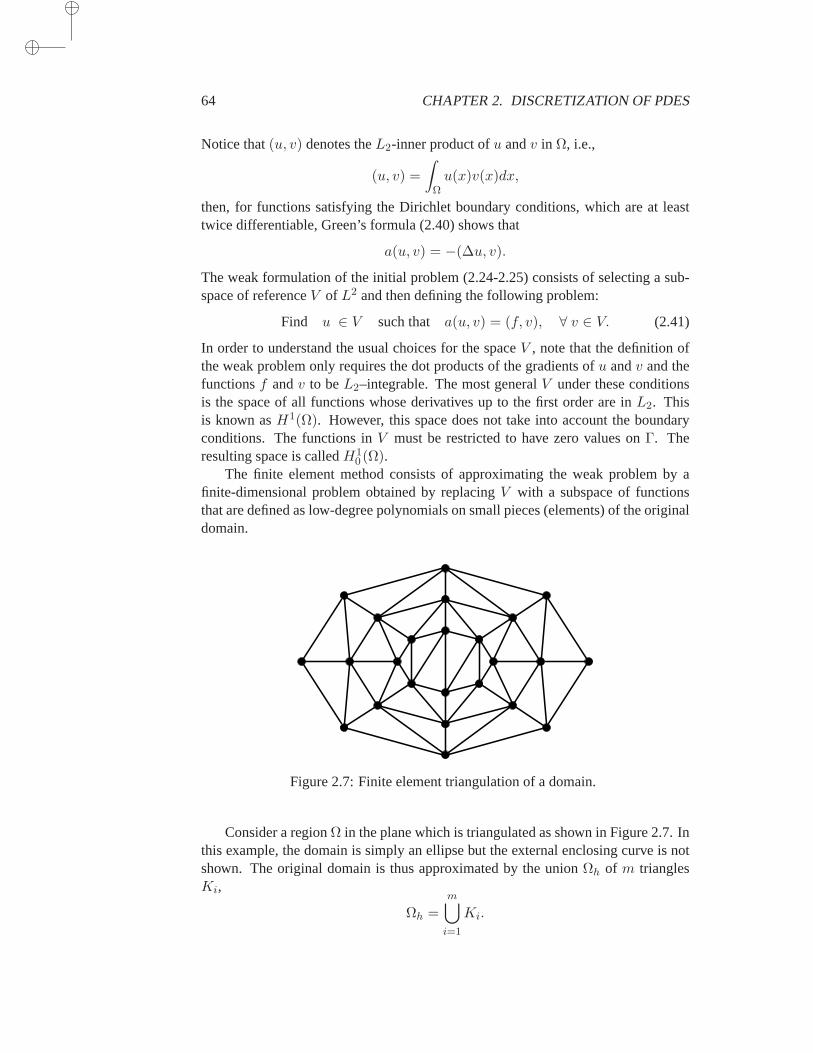
64 CHAPTER 2. DISCRETIZATION OF PDES
Notice that(u, v) denotes theL2-inner product ofu andv in Ω, i.e.,
(u, v) =
∫
Ωu(x)v(x)dx,
then, for functions satisfying the Dirichlet boundary conditions, which are at leasttwice differentiable, Green’s formula (2.40) shows that
a(u, v) = −(∆u, v).
The weak formulation of the initial problem (2.24-2.25) consists of selecting asub-space of referenceV of L2 and then defining the following problem:
Find u ∈ V such that a(u, v) = (f, v), ∀ v ∈ V. (2.41)
In order to understand the usual choices for the spaceV , note that the definition ofthe weak problem only requires the dot products of the gradients ofu andv and thefunctionsf andv to beL2–integrable. The most generalV under these conditionsis the space of all functions whose derivatives up to the first order arein L2. Thisis known asH1(Ω). However, this space does not take into account the boundaryconditions. The functions inV must be restricted to have zero values onΓ. Theresulting space is calledH1
0 (Ω).The finite element method consists of approximating the weak problem by a
finite-dimensional problem obtained by replacingV with a subspace of functionsthat are defined as low-degree polynomials on small pieces (elements) of theoriginaldomain.
Figure 2.7: Finite element triangulation of a domain.
Consider a regionΩ in the plane which is triangulated as shown in Figure 2.7. Inthis example, the domain is simply an ellipse but the external enclosing curve is notshown. The original domain is thus approximated by the unionΩh of m trianglesKi,
Ωh =m⋃
i=1
Ki.
2.3. THE FINITE ELEMENT METHOD 65
For the triangulation to be valid, these triangles must have no vertex that lies ontheedge of any other triangle. Themesh sizeh is defined by
h = maxi=1,...,m
diam(Ki)
where diam(K), the diameter of a triangleK, is the length of its longest side.Then the finite dimensional spaceVh is defined as the space of all functions
which are piecewise linear and continuous on the polygonal regionΩh, and whichvanish on the boundaryΓ. More specifically,
Vh = φ | φ|Ωhcontinuous, φ|Γh
= 0, φ|Kjlinear∀ j.
Here,φ|X represents the restriction of the functionφ to the subsetX. If xj , j =1, . . . , n are the nodes of the triangulation, then a functionφj in Vh can be associ-ated with each nodexj , so that the family of functionsφj ’s satisfies the followingconditions:
φj(xi) = δij =
1 if xi = xj
0 if xi 6= xj. (2.42)
These conditions defineφi, i = 1, . . . , n uniquely. In addition, theφi’s form a basisof the spaceVh.
Each function ofVh can be expressed as
φ(x) =n∑
i=1
ξiφi(x).
The finite element approximation consists of writing the Galerkin condition (2.41)for functions inVh. This defines the approximate problem:
Find u ∈ Vh such that a(u, v) = (f, v), ∀ v ∈ Vh. (2.43)
Sinceu is in Vh, there aren degrees of freedom. By the linearity ofa with respectto v, it is only necessary to impose the conditiona(u, φi) = (f, φi) for i = 1, . . . , n.This results inn constraints.
Writing the desired solutionu in the basisφi as
u =n∑
j=1
ξjφj(x)
and substituting in (2.43) gives the linear problem
n∑
j=1
αijξj = βi (2.44)
whereαij = a(φi, φj), βi = (f, φi).
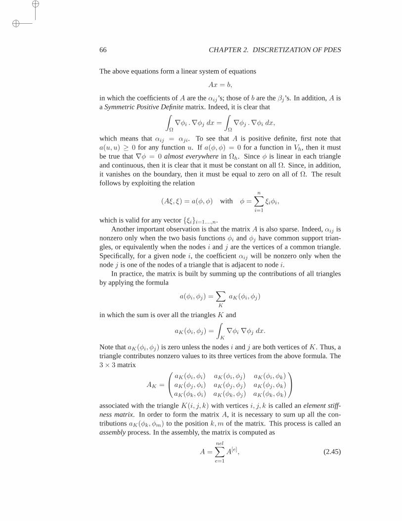
66 CHAPTER 2. DISCRETIZATION OF PDES
The above equations form a linear system of equations
Ax = b,
in which the coefficients ofA are theαij ’s; those ofb are theβj ’s. In addition,A isaSymmetric Positive Definitematrix. Indeed, it is clear that
∫
Ω∇φi .∇φj dx =
∫
Ω∇φj .∇φi dx,
which means thatαij = αji. To see thatA is positive definite, first note thata(u, u) ≥ 0 for any functionu. If a(φ, φ) = 0 for a function inVh, then it mustbe true that∇φ = 0 almost everywherein Ωh. Sinceφ is linear in each triangleand continuous, then it is clear that it must be constant on allΩ. Since, in addition,it vanishes on the boundary, then it must be equal to zero on all ofΩ. The resultfollows by exploiting the relation
(Aξ, ξ) = a(φ, φ) with φ =n∑
i=1
ξiφi,
which is valid for any vectorξii=1....,n.Another important observation is that the matrixA is also sparse. Indeed,αij is
nonzero only when the two basis functionsφi andφj have common support trian-gles, or equivalently when the nodesi andj are the vertices of a common triangle.Specifically, for a given nodei, the coefficientαij will be nonzero only when thenodej is one of the nodes of a triangle that is adjacent to nodei.
In practice, the matrix is built by summing up the contributions of all trianglesby applying the formula
a(φi, φj) =∑
K
aK(φi, φj)
in which the sum is over all the trianglesK and
aK(φi, φj) =
∫
K∇φi ∇φj dx.
Note thataK(φi, φj) is zero unless the nodesi andj are both vertices ofK. Thus, atriangle contributes nonzero values to its three vertices from the above formula. The3× 3 matrix
AK =
aK(φi, φi) aK(φi, φj) aK(φi, φk)aK(φj , φi) aK(φj , φj) aK(φj , φk)aK(φk, φi) aK(φk, φj) aK(φk, φk)
associated with the triangleK(i, j, k) with verticesi, j, k is called anelement stiff-ness matrix. In order to form the matrixA, it is necessary to sum up all the con-tributionsaK(φk, φm) to the positionk,m of the matrix. This process is called anassemblyprocess. In the assembly, the matrix is computed as
A =nel∑
e=1
A[e], (2.45)
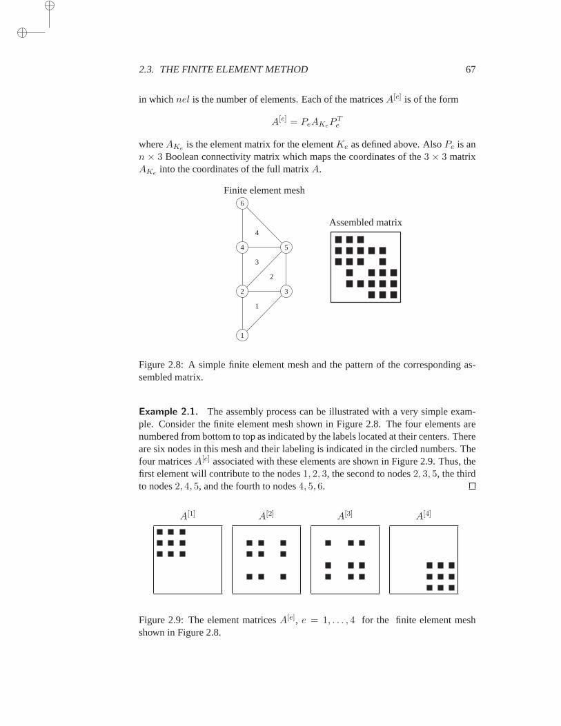
2.3. THE FINITE ELEMENT METHOD 67
in whichnel is the number of elements. Each of the matricesA[e] is of the form
A[e] = PeAKePTe
whereAKe is the element matrix for the elementKe as defined above. AlsoPe is ann × 3 Boolean connectivity matrix which maps the coordinates of the3 × 3 matrixAKe into the coordinates of the full matrixA.
Finite element mesh
1
2 3
4 5
6
1
2
3
4Assembled matrix
Figure 2.8: A simple finite element mesh and the pattern of the corresponding as-sembled matrix.
Example 2.1. The assembly process can be illustrated with a very simple exam-ple. Consider the finite element mesh shown in Figure 2.8. The four elements arenumbered from bottom to top as indicated by the labels located at their centers.Thereare six nodes in this mesh and their labeling is indicated in the circled numbers. Thefour matricesA[e] associated with these elements are shown in Figure 2.9. Thus, thefirst element will contribute to the nodes1, 2, 3, the second to nodes2, 3, 5, the thirdto nodes2, 4, 5, and the fourth to nodes4, 5, 6.
A[1] A[2] A[3] A[4]
Figure 2.9: The element matricesA[e], e = 1, . . . , 4 for the finite element meshshown in Figure 2.8.
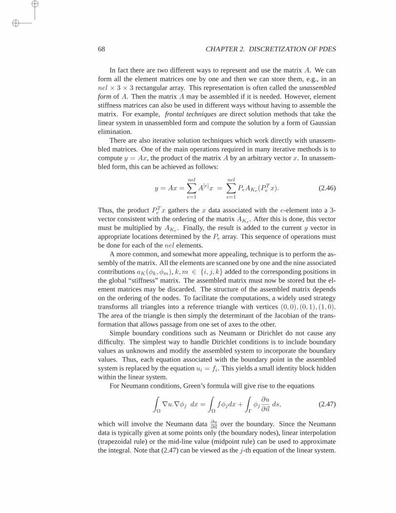
68 CHAPTER 2. DISCRETIZATION OF PDES
In fact there are two different ways to represent and use the matrixA. We canform all the element matrices one by one and then we can store them, e.g., in annel × 3 × 3 rectangular array. This representation is often called theunassembledform of A. Then the matrixA may be assembled if it is needed. However, elementstiffness matrices can also be used in different ways without having to assemble thematrix. For example,frontal techniquesare direct solution methods that take thelinear system in unassembled form and compute the solution by a form of Gaussianelimination.
There are also iterative solution techniques which work directly with unassem-bled matrices. One of the main operations required in many iterative methods is tocomputey = Ax, the product of the matrixA by an arbitrary vectorx. In unassem-bled form, this can be achieved as follows:
y = Ax =
nel∑
e=1
A[e]x =
nel∑
e=1
PeAKe(PTe x). (2.46)
Thus, the productP Te x gathers thex data associated with thee-element into a 3-
vector consistent with the ordering of the matrixAKe . After this is done, this vectormust be multiplied byAKe . Finally, the result is added to the currenty vector inappropriate locations determined by thePe array. This sequence of operations mustbe done for each of thenel elements.
A more common, and somewhat more appealing, technique is to perform the as-sembly of the matrix. All the elements are scanned one by one and the nine associatedcontributionsaK(φk, φm), k,m ∈ i, j, k added to the corresponding positions inthe global “stiffness” matrix. The assembled matrix must now be stored but theel-ement matrices may be discarded. The structure of the assembled matrix dependson the ordering of the nodes. To facilitate the computations, a widely used strategytransforms all triangles into a reference triangle with vertices(0, 0), (0, 1), (1, 0).The area of the triangle is then simply the determinant of the Jacobian of the trans-formation that allows passage from one set of axes to the other.
Simple boundary conditions such as Neumann or Dirichlet do not cause anydifficulty. The simplest way to handle Dirichlet conditions is to include boundaryvalues as unknowns and modify the assembled system to incorporate the boundaryvalues. Thus, each equation associated with the boundary point in the assembledsystem is replaced by the equationui = fi. This yields a small identity block hiddenwithin the linear system.
For Neumann conditions, Green’s formula will give rise to the equations∫
Ω∇u.∇φj dx =
∫
Ωfφjdx+
∫
Γφj∂u
∂~nds, (2.47)
which will involve the Neumann data∂u∂~n over the boundary. Since the Neumann
data is typically given at some points only (the boundary nodes), linear interpolation(trapezoidal rule) or the mid-line value (midpoint rule) can be used to approximatethe integral. Note that (2.47) can be viewed as thej-th equation of the linear system.

2.4. MESH GENERATION AND REFINEMENT 69
Another important point is that if the boundary conditions are only of Neumann type,then the resulting system is singular. An equation must be removed, or the linearsystem must be solved by taking this singularity into account.
2.4 Mesh Generation and Refinement
Generating a finite element triangulation can be done easily by exploiting some initialgrid and then refining the mesh a few times either uniformly or in specific areas.Thesimplest refinement technique consists of taking the three midpoints of a triangle,thus creating four smaller triangles from a larger triangle and losing one triangle,namely, the original one. A systematic use of one level of this strategy is illustratedfor the mesh in Figure 2.8, and is shown in Figure 2.10.
This approach has the advantage of preserving the angles of the original triangu-lation. This is an important property since the angles of a good quality triangulationmust satisfy certain bounds. On the other hand, the indiscriminate use of the uniformrefinement strategy may lead to some inefficiencies. It is desirable to introduce moretriangles in areas where the solution is likely to have large variations. In terms of ver-tices, midpoints should be introduced only where needed. To obtain standard finiteelement triangles, the points that have been created on the edges of a triangle mustbe linked to existing vertices in the triangle. This is because no vertex of a triangle isallowed to lie on the edge of another triangle.
Figure 2.11 shows three possible cases that can arise. The original triangle is (a).In (b), only one new vertex (numbered4) has appeared on one edge of the triangleand it is joined to the vertex opposite to it. In (c), two new vertices appear inside theoriginal triangle. There is no alternative but to join vertices (4) and (5). However,after this is done, either vertices (4) and (3) or vertices (1) and (5) mustbe joined.If angles are desired that will not become too small with further refinements,thesecond choice is clearly better in this case. In fact, various strategies forimprovingthe quality of the triangles have been devised. The final case (d) corresponds to the“uniform refinement” case where all edges have been split in two. Thereare threenew vertices and four new elements, and the larger initial element is removed.
2.5 Finite Volume Method
The finite volume method is geared toward the solution of conservation laws of theform:
∂u
∂t+∇. ~F = Q. (2.48)
In the above equation,~F (u, t) is a certain vector function ofu and time, possiblynonlinear. This is called the “flux vector.” Thesource termQ is a function of spaceand time. We now apply the principle used in the weak formulation, described before.Multiply both sides by a test functionw, and take the integral
∫
Ωw∂u
∂tdx+
∫
Ωw ∇. ~F dx =
∫
Ωw Q dx.
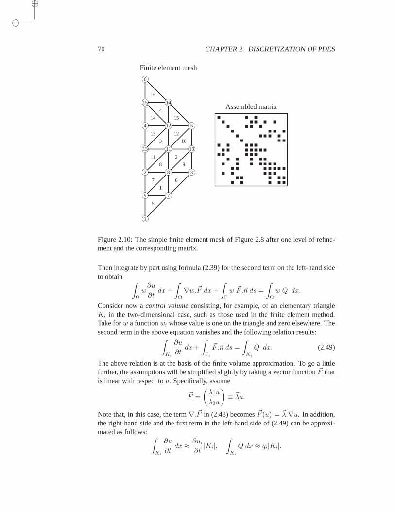
70 CHAPTER 2. DISCRETIZATION OF PDES
Finite element mesh
1
2 3
4 5
6
7
8
9
1011
12
13
1415
1
2
3
4
5
67
8 9
10
11
1213
14 15
16
Assembled matrix
Figure 2.10: The simple finite element mesh of Figure 2.8 after one level of refine-ment and the corresponding matrix.
Then integrate by part using formula (2.39) for the second term on the left-hand sideto obtain
∫
Ωw∂u
∂tdx−
∫
Ω∇w.~F dx+
∫
Γw ~F .~n ds =
∫
Ωw Q dx.
Consider now acontrol volumeconsisting, for example, of an elementary triangleKi in the two-dimensional case, such as those used in the finite element method.Take forw a functionwi whose value is one on the triangle and zero elsewhere. Thesecond term in the above equation vanishes and the following relation results:
∫
Ki
∂u
∂tdx+
∫
Γi
~F .~n ds =
∫
Ki
Q dx. (2.49)
The above relation is at the basis of the finite volume approximation. To go a littlefurther, the assumptions will be simplified slightly by taking a vector function~F thatis linear with respect tou. Specifically, assume
~F =
(λ1u
λ2u
)
≡ ~λu.
Note that, in this case, the term∇. ~F in (2.48) becomes~F (u) = ~λ.∇u. In addition,the right-hand side and the first term in the left-hand side of (2.49) can be approxi-mated as follows:
∫
Ki
∂u
∂tdx ≈ ∂ui
∂t|Ki|,
∫
Ki
Q dx ≈ qi|Ki|.
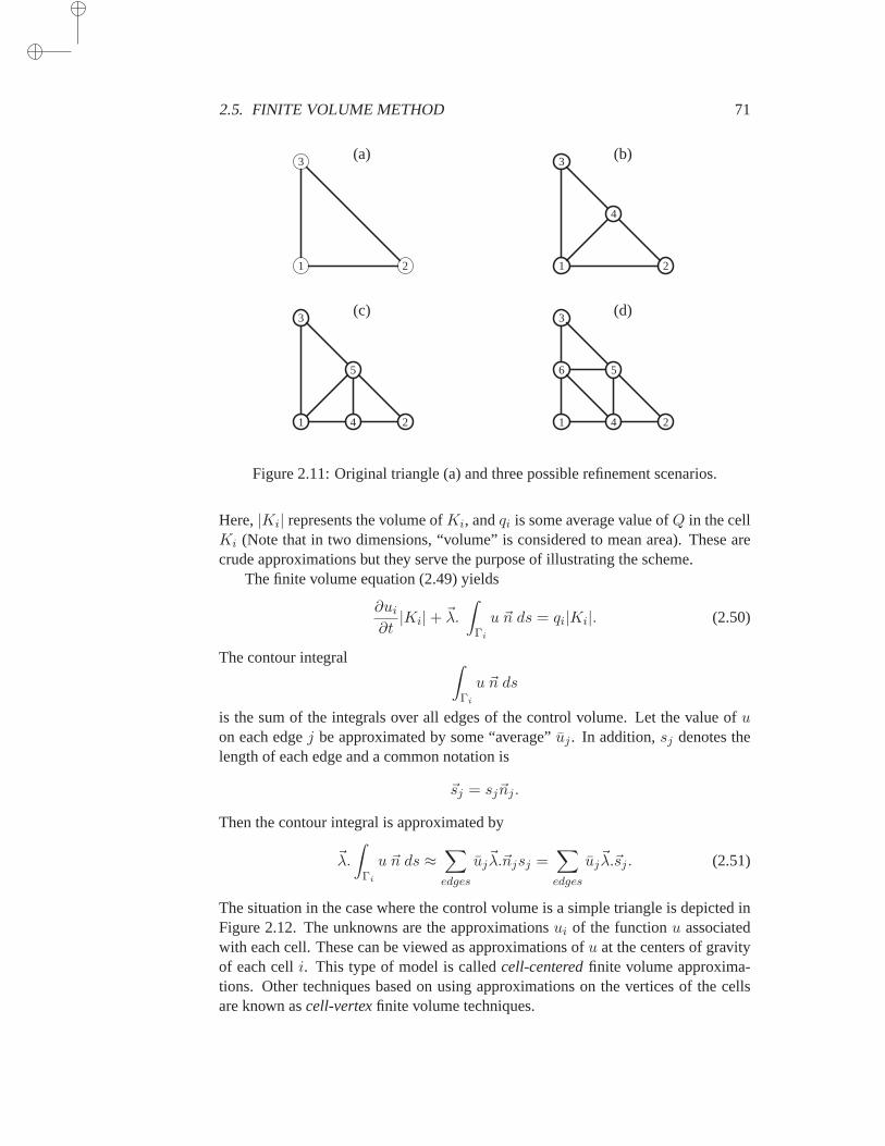
2.5. FINITE VOLUME METHOD 71
(a)
1 2
3(b)
1 2
3
4
(c)
1 2
3
4
5
(d)
1 2
3
4
56
Figure 2.11: Original triangle (a) and three possible refinement scenarios.
Here,|Ki| represents the volume ofKi, andqi is some average value ofQ in the cellKi (Note that in two dimensions, “volume” is considered to mean area). These arecrude approximations but they serve the purpose of illustrating the scheme.
The finite volume equation (2.49) yields
∂ui
∂t|Ki|+ ~λ.
∫
Γi
u ~n ds = qi|Ki|. (2.50)
The contour integral ∫
Γi
u ~n ds
is the sum of the integrals over all edges of the control volume. Let the valueof uon each edgej be approximated by some “average”uj . In addition,sj denotes thelength of each edge and a common notation is
~sj = sj~nj .
Then the contour integral is approximated by
~λ.
∫
Γi
u ~n ds ≈∑
edges
uj~λ.~njsj =
∑
edges
uj~λ.~sj . (2.51)
The situation in the case where the control volume is a simple triangle is depicted inFigure 2.12. The unknowns are the approximationsui of the functionu associatedwith each cell. These can be viewed as approximations ofu at the centers of gravityof each celli. This type of model is calledcell-centeredfinite volume approxima-tions. Other techniques based on using approximations on the vertices of thecellsare known ascell-vertexfinite volume techniques.
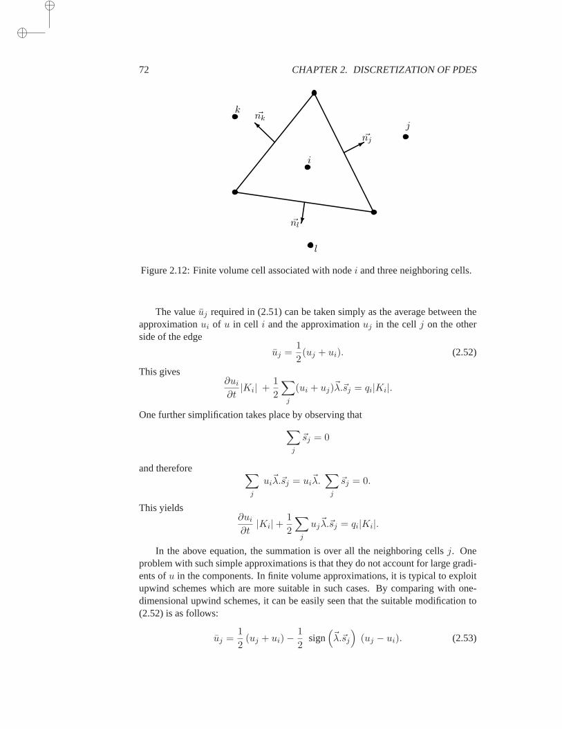
72 CHAPTER 2. DISCRETIZATION OF PDES
*~nj
~nl
I~nk
i
j
k
l
Figure 2.12: Finite volume cell associated with nodei and three neighboring cells.
The valueuj required in (2.51) can be taken simply as the average between theapproximationui of u in cell i and the approximationuj in the cellj on the otherside of the edge
uj =1
2(uj + ui). (2.52)
This gives∂ui
∂t|Ki| +
1
2
∑
j
(ui + uj)~λ.~sj = qi|Ki|.
One further simplification takes place by observing that∑
j
~sj = 0
and therefore ∑
j
ui~λ.~sj = ui
~λ.∑
j
~sj = 0.
This yields∂ui
∂t|Ki|+
1
2
∑
j
uj~λ.~sj = qi|Ki|.
In the above equation, the summation is over all the neighboring cellsj. Oneproblem with such simple approximations is that they do not account for largegradi-ents ofu in the components. In finite volume approximations, it is typical to exploitupwind schemes which are more suitable in such cases. By comparing with one-dimensional upwind schemes, it can be easily seen that the suitable modificationto(2.52) is as follows:
uj =1
2(uj + ui)−
1
2sign
(
~λ.~sj
)
(uj − ui). (2.53)
2.5. FINITE VOLUME METHOD 73
This gives
∂ui
∂t|Ki|+
∑
j
~λ.~sj
(1
2(uj + ui)−
1
2sign(~λ.~sj)(uj − ui)
)
= qi|Ki|.
Now write
∂ui
∂t|Ki| +
∑
j
(1
2(uj + ui)~λ.~sj −
1
2|~λ.~sj |(uj − ui)
)
= qi|Ki|
∂ui
∂t|Ki| +
∑
j
(
ui(~λ.~sj)+ + uj(~λ.~sj)
−)
= qi|Ki|
where
(z)± ≡ z ± |z|2
.
The equation for celli takes the form
∂ui
∂t|Ki|+ βiui +
∑
j
αijuj = qi|Ki|,
where
βi =∑
j
(~λ.~sj)+ ≥ 0, (2.54)
αij = (~λ.~sj)− ≤ 0. (2.55)
Thus, the diagonal elements of the matrix are nonnegative, while its offdiagonalelements are nonpositive. In addition, the row-sum of the elements, i.e., the sum ofall elements in the same row, is equal to zero. This is because
βi +∑
j
αij =∑
j
(~λ.~sj)+ +
∑
j
(~λ.~sj)− =
∑
j
~λ.~sj = ~λ.∑
j
~sj = 0.
The matrices obtained have the same desirable property of weak diagonal dominanceseen in the one-dimensional case. A disadvantage of upwind schemes, whether in thecontext of irregular grids or in one-dimensional equations, is the loss of accuracy dueto the low order of the schemes.
PROBLEMS
P-2.1 Derive Forward Difference formulas similar to (2.8), i.e.,involving u(x), u(x +h), u(x + 2h), . . ., which are of second and third order. Write down the discretization er-rors explicitly.
P-2.2 Derive a Centered Difference formula for the first derivative, similar to (2.13), whichis at least of third order.
74 CHAPTER 2. DISCRETIZATION OF PDES
P-2.3 Show that the Upwind Difference scheme described in 2.2.4, whena and~b are con-stant, is stable for the model problem (2.7).
P-2.4 Develop the two nine-point formulas illustrated in Figure 2.4. Find the correspondingdiscretization errors. [Hint: Combine13 of the five-point formula (2.17) plus23 of the sameformula based on the diagonal stencil(x, y), (x+ h, y + h) + (x+ h, y − h), (x− h, y +h), (x − h, y − h) to get one formula. Use the reverse combination2
3 , 13 to get the other
formula.]
P-2.5 Consider a (two-dimensional) rectangular mesh which is discretized as in the finitedifference approximation. Show that the finite volume approximation to~λ.∇u yields thesame matrix as an upwind scheme applied to the same problem. What would be the mesh ofthe equivalent upwind finite difference approximation?
P-2.6 Show that the right-hand side of equation (2.16) can also be written as
1
h2δ−(
ai+ 1
2
δ+u)
.
P-2.7 Show that the formula (2.16) is indeed second order accuratefor functions that are inC4.
P-2.8 Show that the functionsφi’s defined by (2.42) form a basis ofVh.
P-2.9 Develop the equivalent of Green’s formula for the elliptic operatorL defined in (2.6).
P-2.10 Write a short FORTRAN or C program to perform a matrix-by-vector product whenthe matrix is stored in unassembled form.
P-2.11 Consider the finite element mesh of Example 2.1. Compare the number of opera-tions required to perform a matrix-by-vector product when the matrix is in assembled andin unassembled form. Compare also the storage required in each case. For a general finiteelement matrix, what can the ratio be between the two in the worst case (consider only linearapproximations on triangular elements) for arithmetic? Express the number of operations interms of the number of nodes and edges of the mesh. You may makethe assumption that themaximum number of elements that are adjacent to a given node isp (e.g.,p = 8).
P-2.12 LetK be a polygon inR2 withm edges, and let~sj = sj~nj , for j = 1, . . . ,m, wheresj is the length of thej-th edge and~nj is the unit outward normal at thej-th edge. Use thedivergence theorem to prove that
∑mj=1 ~sj = 0.
NOTES AND REFERENCES. The books by C. Johnson [179], P. Ciarlet [84], and G. Strang andG.Fix [277] are recommended for a good coverage of the finite element method. Axelsson and Barker[15] discuss solution techniques for finite element problems emphasizingiterative methods. For finitedifference and finite volume methods, see C. Hirsch’s book [168] which also discusses equations andsolution methods for fluid flow problems. A 1965 article by Hockney [169]describes a one-level blockcyclic reduction method which seems to be the first “Fast Poisson Solver”. Block cyclic reduction wasdeveloped by Buneman [69] and Hockney [171] for Poisson’s equations, and extended by Swartzrauber[279] to separable elliptic equations. An efficient combination of block cyclic reduction and Fourieranalysis known as FACR(l), was developed by Hockney [171] and laterextended in [280] and [170].Parallel block cyclic reduction algorithms were considered in [138, 281].
Chapter 3
SPARSE MATRICES
As described in the previous chapter, standard discretizations of Partial Differential Equations
typically lead to large and sparse matrices. A sparse matrix is defined, somewhat vaguely, as
a matrix which has very few nonzero elements. But, in fact, a matrix can be termed sparse
whenever special techniques can be utilized to take advantage of the large number of zero
elements and their locations. These sparse matrix techniques begin with the idea that the
zero elements need not be stored. One of the key issues is to define data structures for these
matrices that are well suited for efficient implementation of standard solution methods, whether
direct or iterative. This chapter gives an overview of sparse matrices, their properties, their
representations, and the data structures used to store them.
3.1 Introduction
The natural idea to take advantage of the zeros of a matrix and their location was ini-tiated by engineers in various disciplines. In the simplest case involving banded ma-trices, special techniques are straightforward to develop. Electrical engineers dealingwith electrical networks in the 1960s were the first to exploit sparsity to solvegeneralsparse linear systems for matrices with irregular structure. The main issue, and thefirst addressed by sparse matrix technology, was to devise direct solution methodsfor linear systems. These had to be economical, both in terms of storage and compu-tational effort. Sparse direct solvers can handle very large problems that cannot betackled by the usual “dense” solvers.
Essentially, there are two broad types of sparse matrices:structuredandunstruc-tured. A structured matrix is one whose nonzero entries form a regular pattern,oftenalong a small number of diagonals. Alternatively, the nonzero elements may lie inblocks (dense submatrices) of the same size, which form a regular pattern, typicallyalong a small number of (block) diagonals. A matrix with irregularly located entriesis said to be irregularly structured. The best example of a regularly structured ma-trix is a matrix that consists of only a few diagonals. Finite difference matrices onrectangular grids, such as the ones seen in the previous chapter, are typical examplesof matrices with regular structure. Most finite element or finite volume techniques
75
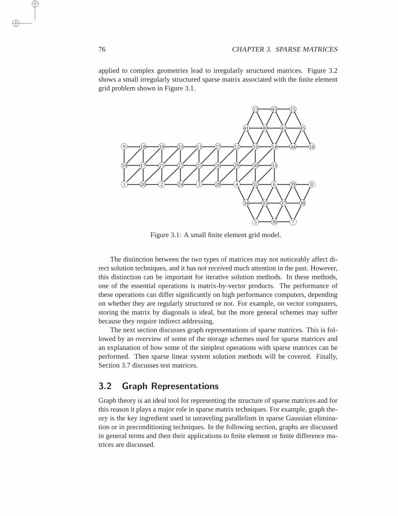
76 CHAPTER 3. SPARSE MATRICES
applied to complex geometries lead to irregularly structured matrices. Figure 3.2shows a small irregularly structured sparse matrix associated with the finite elementgrid problem shown in Figure 3.1.
1 2 3 4
5
6
7
8
9 10 11 12
13
14
15
16
17
18
19
20
21 22
23
24
25 26
27
28
29 30
31
32
33
34 35
36
37 38
39
4041 42
43
44
45
Figure 3.1: A small finite element grid model.
The distinction between the two types of matrices may not noticeably affect di-rect solution techniques, and it has not received much attention in the past.However,this distinction can be important for iterative solution methods. In these methods,one of the essential operations is matrix-by-vector products. The performance ofthese operations can differ significantly on high performance computers,dependingon whether they are regularly structured or not. For example, on vector computers,storing the matrix by diagonals is ideal, but the more general schemes may sufferbecause they require indirect addressing.
The next section discusses graph representations of sparse matrices.This is fol-lowed by an overview of some of the storage schemes used for sparse matrices andan explanation of how some of the simplest operations with sparse matrices canbeperformed. Then sparse linear system solution methods will be covered. Finally,Section 3.7 discusses test matrices.
3.2 Graph Representations
Graph theory is an ideal tool for representing the structure of sparse matrices and forthis reason it plays a major role in sparse matrix techniques. For example, graph the-ory is the key ingredient used in unraveling parallelism in sparse Gaussianelimina-tion or in preconditioning techniques. In the following section, graphs are discussedin general terms and then their applications to finite element or finite differencema-trices are discussed.
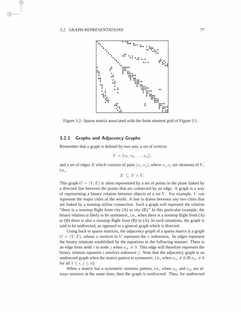
3.2. GRAPH REPRESENTATIONS 77
Figure 3.2: Sparse matrix associated with the finite element grid of Figure 3.1.
3.2.1 Graphs and Adjacency Graphs
Remember that a graph is defined by two sets, a set of vertices
V = v1, v2, . . . , vn,
and a set of edgesE which consists of pairs(vi, vj), wherevi, vj are elements ofV ,i.e.,
E ⊆ V × V.This graphG = (V,E) is often represented by a set of points in the plane linked bya directed line between the points that are connected by an edge. A graph isa wayof representing a binary relation between objects of a setV . For example,V canrepresent the major cities of the world. A line is drawn between any two cities thatare linked by a nonstop airline connection. Such a graph will represent the relation“there is a nonstop flight from city (A) to city (B).” In this particular example,thebinary relation is likely to be symmetric, i.e., when there is a nonstop flight from (A)to (B) there is also a nonstop flight from (B) to (A). In such situations, the graph issaid to be undirected, as opposed to a general graph which is directed.
Going back to sparse matrices, theadjacency graphof a sparse matrix is a graphG = (V,E), whosen vertices inV represent then unknowns. Its edges representthe binary relations established by the equations in the following manner: There isan edge from nodei to nodej whenaij 6= 0. This edge will therefore represent thebinary relationequationi involves unknownj. Note that the adjacency graph is anundirected graph when the matrix pattern is symmetric, i.e., whenaij 6= 0 iff aji 6= 0for all 1 ≤ i, j ≤ n).
When a matrix has a symmetric nonzero pattern, i.e., whenaij andaji are al-ways nonzero at the same time, then the graph isundirected. Thus, for undirected

78 CHAPTER 3. SPARSE MATRICES
graphs, every edge points in both directions. As a result, undirected graphs can berepresented with nonoriented edges.
As an example of the use of graph models, parallelism in Gaussian eliminationcan be extracted by finding unknowns that are independent at a givenstage of theelimination. These are unknowns which do not depend on each other according to theabove binary relation. The rows corresponding to such unknowns canthen be usedas pivots simultaneously. Thus, in one extreme, when the matrix is diagonal, then allunknowns are independent. Conversely, when a matrix is dense, each unknown willdepend on all other unknowns. Sparse matrices lie somewhere between these twoextremes.
1 2
4 3
1 2
4 3
Figure 3.3: Graphs of two4× 4 sparse matrices.
There are a few interesting simple properties of adjacency graphs. The graphof A2 can be interpreted as ann-vertex graph whose edges are the pairs(i, j) forwhich there exists at least one path of length exactly two from nodei to nodej inthe original graph ofA. Similarly, the graph ofAk consists of edges which representthe binary relation “there is at least one path of lengthk from nodei to nodej.” Fordetails, see Exercise 4.
3.2.2 Graphs of PDE Matrices
For Partial Differential Equations involving only one physical unknown per meshpoint, the adjacency graph of the matrix arising from the discretization is oftenthegraph represented by the mesh itself. However, it is common to have several un-knowns per mesh point. For example, the equations modeling fluid flow may involvethe two velocity components of the fluid (in two dimensions) as well as energy andmomentum at each mesh point.
In such situations, there are two choices when labeling the unknowns. Theycan be labeled contiguously at each mesh point. Thus, for the example just men-

3.3. PERMUTATIONS AND REORDERINGS 79
tioned, we can label all four variables (two velocities followed by momentum andthen pressure) at a given mesh point asu(k), . . ., u(k + 3). Alternatively, all un-knowns associated with one type of variable can be labeled first (e.g., first velocitycomponents), followed by those associated with the second type of variables (e.g.,second velocity components), etc. In either case, it is clear that there is redundantinformation in the graph of the adjacency matrix.
Thequotientgraph corresponding to thephysical meshcan be used instead. Thisresults in substantial savings in storage and computation. In the fluid flow examplementioned above, the storage can be reduced by a factor of almost 16 forthe integerarrays needed to represent the graph. This is because the number of edges has beenreduced by this much, while the number of vertices, which is usually much smaller,remains the same.
3.3 Permutations and Reorderings
Permuting the rows or the columns, or both the rows and columns, of a sparsematrixis a common operation. In fact,reordering rows and columns is one of the mostimportant ingredients used inparallel implementations of both direct and iterativesolution techniques. This section introduces the ideas related to these reorderingtechniques and their relations to the adjacency graphs of the matrices. Recall thenotation introduced in Chapter 1 that thej-th column of a matrix is denoted bya∗jand thei-th row byai∗.
3.3.1 Basic Concepts
We begin with a definition and new notation.
Definition 3.1 LetA be a matrix andπ = i1, i2, . . . , in a permutation of the set1, 2, . . . , n. Then the matrices
Aπ,∗ = aπ(i),ji=1,...,n;j=1,...,m,
A∗,π = ai,π(j)i=1,...,n;j=1,...,m
are called rowπ-permutation and columnπ-permutation ofA, respectively.
It is well known that any permutation of the set1, 2, . . . , n results from at mostn interchanges, i.e., elementary permutations in which only two entries have beeninterchanged. Aninterchange matrixis the identity matrix with two of its rows in-terchanged. Denote byXij such matrices, withi and j being the numbers of theinterchanged rows. Note that in order to interchange rowsi andj of a matrixA, weonly need to premultiply it by the matrixXij . Let π = i1, i2, . . . , in be an arbi-trary permutation. This permutation is the product of a sequence ofn consecutiveinterchangesσ(ik, jk), k = 1, . . . , n. Then the rows of a matrix can be permuted byinterchanging rowsi1, j1, then rowsi2, j2 of the resulting matrix, etc., and finally byinterchangingin, jn of the resulting matrix. Each of these operations can be achieved
80 CHAPTER 3. SPARSE MATRICES
by a premultiplication byXik,jk. The same observation can be made regarding the
columns of a matrix: In order to interchange columnsi andj of a matrix, postmulti-ply it by Xij . The following proposition follows from these observations.
Proposition 3.2 Let π be a permutation resulting from the product of the inter-changesσ(ik, jk), k = 1, . . . , n. Then,
Aπ,∗ = PπA, A∗,π = AQπ,
where
Pπ = Xin,jnXin−1,jn−1 . . . Xi1,j1 , (3.1)
Qπ = Xi1,j1Xi2,j2 . . . Xin,jn . (3.2)
Products of interchange matrices are calledpermutation matrices. Clearly, a permu-tation matrix is nothing but the identity matrix with its rows (or columns) permuted.
Observe thatX2i,j = I, i.e., the square of an interchange matrix is the identity, or
equivalently, the inverse of an interchange matrix is equal to itself, a property whichis intuitively clear. It is easy to see that the matrices (3.1) and (3.2) satisfy
PπQπ = Xin,jnXin−1,jn−1 . . . Xi1,j1 ×Xi1,j1Xi2,j2 . . . Xin,jn = I,
which shows that the two matricesQπ andPπ are nonsingular and that they are theinverse of one another. In other words, permuting the rows and the columns of a ma-trix, using the same permutation, actually performs a similarity transformation. An-other important consequence arises because the products involved in thedefinitions(3.1) and (3.2) ofPπ andQπ occur in reverse order. Since each of the elementarymatricesXik,jk
is symmetric, the matrixQπ is the transpose ofPπ. Therefore,
Qπ = P Tπ = P−1
π .
Since the inverse of the matrixPπ is its own transpose, permutation matrices areunitary.
Another way of deriving the above relationships is to express the permutationmatricesPπ andP T
π in terms of the identity matrix, whose columns or rows arepermuted. It can easily be seen (See Exercise 3) that
Pπ = Iπ,∗, P Tπ = I∗,π.
It is then possible to verify directly that
Aπ,∗ = Iπ,∗A = PπA, A∗,π = AI∗,π = AP Tπ .
It is important to interpret permutation operations for the linear systems to besolved. When the rows of a matrix are permuted, the order in which the equationsare written is changed. On the other hand, when the columns are permuted, theunknowns are in effectrelabeled, or reordered.
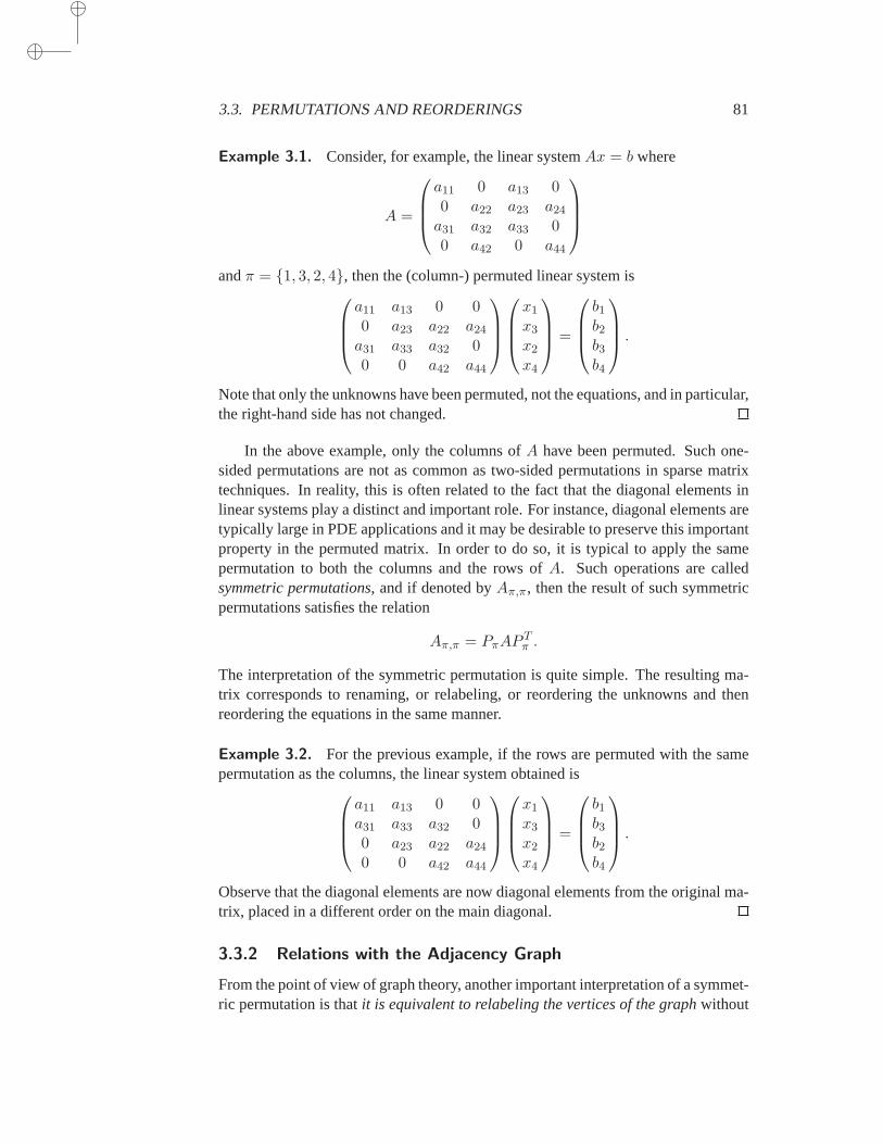
3.3. PERMUTATIONS AND REORDERINGS 81
Example 3.1. Consider, for example, the linear systemAx = b where
A =
a11 0 a13 00 a22 a23 a24
a31 a32 a33 00 a42 0 a44
andπ = 1, 3, 2, 4, then the (column-) permuted linear system is
a11 a13 0 00 a23 a22 a24
a31 a33 a32 00 0 a42 a44
x1
x3
x2
x4
=
b1b2b3b4
.
Note that only the unknowns have been permuted, not the equations, and inparticular,the right-hand side has not changed.
In the above example, only the columns ofA have been permuted. Such one-sided permutations are not as common as two-sided permutations in sparse matrixtechniques. In reality, this is often related to the fact that the diagonal elements inlinear systems play a distinct and important role. For instance, diagonal elements aretypically large in PDE applications and it may be desirable to preserve this importantproperty in the permuted matrix. In order to do so, it is typical to apply the samepermutation to both the columns and the rows ofA. Such operations are calledsymmetric permutations, and if denoted byAπ,π, then the result of such symmetricpermutations satisfies the relation
Aπ,π = PπAPTπ .
The interpretation of the symmetric permutation is quite simple. The resulting ma-trix corresponds to renaming, or relabeling, or reordering the unknowns and thenreordering the equations in the same manner.
Example 3.2. For the previous example, if the rows are permuted with the samepermutation as the columns, the linear system obtained is
a11 a13 0 0a31 a33 a32 00 a23 a22 a24
0 0 a42 a44
x1
x3
x2
x4
=
b1b3b2b4
.
Observe that the diagonal elements are now diagonal elements from the original ma-trix, placed in a different order on the main diagonal.
3.3.2 Relations with the Adjacency Graph
From the point of view of graph theory, another important interpretation ofa symmet-ric permutation is thatit is equivalent to relabeling the vertices of the graphwithout
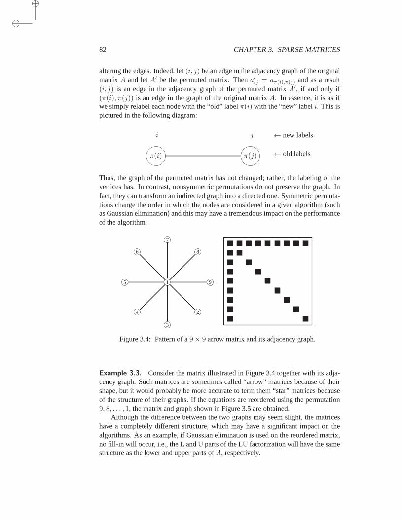
82 CHAPTER 3. SPARSE MATRICES
altering the edges. Indeed, let(i, j) be an edge in the adjacency graph of the originalmatrixA and letA′ be the permuted matrix. Thena′ij = aπ(i),π(j) and as a result(i, j) is an edge in the adjacency graph of the permuted matrixA′, if and only if(π(i), π(j)) is an edge in the graph of the original matrixA. In essence, it is as ifwe simply relabel each node with the “old” labelπ(i) with the “new” labeli. This ispictured in the following diagram:
π(i) π(j)
i j ← new labels
← old labels
Thus, the graph of the permuted matrix has not changed; rather, the labeling of thevertices has. In contrast, nonsymmetric permutations do not preserve the graph. Infact, they can transform an indirected graph into a directed one. Symmetric permuta-tions change the order in which the nodes are considered in a given algorithm (suchas Gaussian elimination) and this may have a tremendous impact on the performanceof the algorithm.
1
2
3
4
5
6
7
8
9
Figure 3.4: Pattern of a 9× 9 arrow matrix and its adjacency graph.
Example 3.3. Consider the matrix illustrated in Figure 3.4 together with its adja-cency graph. Such matrices are sometimes called “arrow” matrices becauseof theirshape, but it would probably be more accurate to term them “star” matrices becauseof the structure of their graphs. If the equations are reordered using the permutation9, 8, . . . , 1, the matrix and graph shown in Figure 3.5 are obtained.
Although the difference between the two graphs may seem slight, the matriceshave a completely different structure, which may have a significant impact on thealgorithms. As an example, if Gaussian elimination is used on the reordered matrix,no fill-in will occur, i.e., the L and U parts of the LU factorization will have the samestructure as the lower and upper parts ofA, respectively.
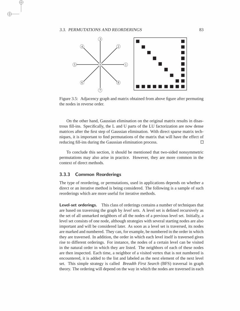
3.3. PERMUTATIONS AND REORDERINGS 83
1
2
3
4
5
6
7
8
9
Figure 3.5: Adjacency graph and matrix obtained from above figure afterpermutingthe nodes in reverse order.
On the other hand, Gaussian elimination on the original matrix results in disas-trous fill-ins. Specifically, the L and U parts of the LU factorization are now densematrices after the first step of Gaussian elimination. With direct sparse matrix tech-niques, it is important to find permutations of the matrix that will have the effect ofreducing fill-ins during the Gaussian elimination process.
To conclude this section, it should be mentioned that two-sided nonsymmetricpermutations may also arise in practice. However, they are more common in thecontext of direct methods.
3.3.3 Common Reorderings
The type of reordering, or permutations, used in applications depends onwhether adirect or an iterative method is being considered. The following is a sample ofsuchreorderings which are more useful for iterative methods.
Level-set orderings. This class of orderings contains a number of techniques thatare based on traversing the graph bylevel sets. A level set is defined recursively asthe set of all unmarked neighbors of all the nodes of a previous level set. Initially, alevel set consists of one node, although strategies with several starting nodes are alsoimportant and will be considered later. As soon as a level set is traversed, its nodesare marked and numbered. They can, for example, be numbered in the order in whichthey are traversed. In addition, the order in which each level itself is traversed givesrise to different orderings. For instance, the nodes of a certain level can be visitedin the natural order in which they are listed. The neighbors of each of these nodesare then inspected. Each time, a neighbor of a visited vertex that is not numbered isencountered, it is added to the list and labeled as the next element of the next levelset. This simple strategy is calledBreadth First Search(BFS) traversal in graphtheory. The ordering will depend on the way in which the nodes are traversed in each
84 CHAPTER 3. SPARSE MATRICES
level set. In BFS the elements of a level set are always traversed in the natural orderin which they are listed. In theCuthill-McKee orderingthe nodes adjacent a a visitednode are always traversed from lowest to highest degree.
ALGORITHM 3.1 BFS(G, v)
1. InitializeS = v, seen = 1, π(seen) = v; Mark v;2. Whileseen < n Do3. Snew = ∅;4. For each nodev in S do5. For each unmarkedw in adj(v) do6. Addw to Snew;7. Markw;8. π(+ + seen) = w;9. EndDo
10. S := Snew
11. EndDo12. EndWhile
In the above algorithm, the notationπ(+ + seen) = w in Line 8, uses a style bor-rowed from the C/C++ language. It states thatseen should be first incremented byone, and thenπ(seen) is assignedw. Two important modifications will be made tothis algorithm to obtain the Cuthill Mc Kee ordering. The first concerns the selectionof the first node to begin the traversal. The second, mentioned above, is the orde inwhich the nearest neighbors of a given node are traversed.
ALGORITHM 3.2 Cuthill-McKee (G)
0. Find an intial nodev for the traversal1. InitializeS = v, seen = 1, π(seen) = v; Mark v;2. Whileseen < n Do3. Snew = ∅;4. For each nodev Do:5. π(+ + seen) = v;6. For each unmarkedw in adj(v), going from lowest to highest degree Do:7. Addw to Snew;8. Markw;9. EndDo
10. S := Snew
11. EndDo12. EndWhile
Theπ array obtained from the procedure lists the nodes in the order in whichthey are visited and can, in a practical implementation, be used to store the levelsetsin succession. A pointer is needed to indicate where each set starts.

3.3. PERMUTATIONS AND REORDERINGS 85
The main property of level sets is that, at the exception of the first and the lastlevels, they are aregraph separators. A graph separator is a set of vertices, theremoval of which separates the graph in two disjoint components. In fact iftherearel levels andV1 = S1US2 . . . Si−1, V2 = Si+1U . . . Sl, then the nodes ofV1 areV2 are not coupled. This is easy to prove by contradiction. A major consequence ofthis property is that the matrix resulting from the Cuthill-McKee (or BFS) orderingis block-tridiagonal, with thei-th block being of size|Si|.
I order to explain the concept of level sets, the previous two algorithms weredescribed with the explicit use of level sets. A more common, and somewhat simpler,implementation relies onqueues. The queue implementation is as follows.
ALGORITHM 3.3 Cuthill-McKee (G) – Queue implementation
0. Find an intial nodev for the traversal1. InitializeQ = v, Mark v;2. While |Q| < n Do3. head+ + ;4. For each unmarkedw in adj(h), going from lowest to highest degree Do:5. Appendw toQ;6. Markw;7. EndDo8. EndWhile
The final arrayQ will give the desired permutationπ. Clearly, this implementationcan also be applied to BFS. As an example, consider the finite element mesh problemillustrated in Figure 2.10 of Chapter 2, and assume thatv = 3 is the initial node ofthe traversal. The state of theQ array after each step along with the head vertexheadand its adjacency list are shown in the following table. Note that the adjacencylistsin the third column are listed by increasing degrees.
Q head adj(head)
3 3 7, 10, 83, 7, 10, 8 7 1, 93, 7, 10, 8, 1, 9 10 5, 113, 7, 10, 8, 1, 9, 5, 11 8 23, 7, 10, 8, 1, 9, 5, 11, 2 1 -3, 7, 10, 8, 1, 9, 5, 11, 2 9 -3, 7, 10, 8, 1, 9, 5, 11, 2 5 14, 123, 7, 10, 8, 1, 9, 5, 11, 2, 14, 12 11 133, 7, 10, 8, 1, 9, 5, 11, 2, 14, 12, 13 2 -3, 7, 10, 8, 1, 9, 5, 11, 2, 14, 12, 13 14 6, 153, 7, 10, 8, 1, 9, 5, 11, 2, 14, 12, 13, 6, 15 12 43, 7, 10, 8, 1, 9, 5, 11, 2, 14, 12, 13, 6, 15, 4
An implementation using explicit levels, would find the setsS1 = 3, S2 =7, 8, 10, S3 = 1, 9, 5, 11, 2, S4 = 14, 12, 13, andS5 = 6, 15, 4. The
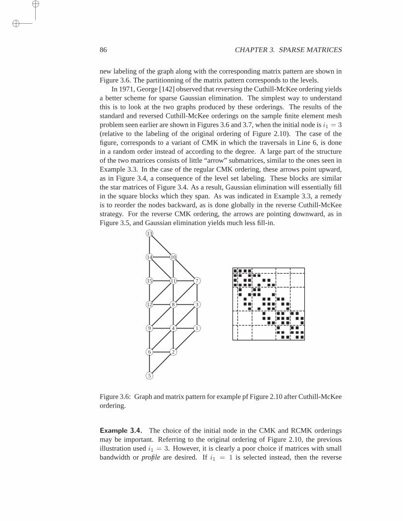
86 CHAPTER 3. SPARSE MATRICES
new labeling of the graph along with the corresponding matrix pattern are shown inFigure 3.6. The partitionning of the matrix pattern corresponds to the levels.
In 1971, George [142] observed thatreversingthe Cuthill-McKee ordering yieldsa better scheme for sparse Gaussian elimination. The simplest way to understandthis is to look at the two graphs produced by these orderings. The results of thestandard and reversed Cuthill-McKee orderings on the sample finite elementmeshproblem seen earlier are shown in Figures 3.6 and 3.7, when the initial nodeis i1 = 3(relative to the labeling of the original ordering of Figure 2.10). The caseof thefigure, corresponds to a variant of CMK in which the traversals in Line 6,is donein a random order instead of according to the degree. A large part of thestructureof the two matrices consists of little “arrow” submatrices, similar to the ones seen inExample 3.3. In the case of the regular CMK ordering, these arrows pointupward,as in Figure 3.4, a consequence of the level set labeling. These blocks are similarthe star matrices of Figure 3.4. As a result, Gaussian elimination will essentially fillin the square blocks which they span. As was indicated in Example 3.3, a remedyis to reorder the nodes backward, as is done globally in the reverse Cuthill-McKeestrategy. For the reverse CMK ordering, the arrows are pointing downward, as inFigure 3.5, and Gaussian elimination yields much less fill-in.
1
2
3
4
5
6
7
8
9
10
11
12
13
14
15
Figure 3.6: Graph and matrix pattern for example pf Figure 2.10 after Cuthill-McKeeordering.
Example 3.4. The choice of the initial node in the CMK and RCMK orderingsmay be important. Referring to the original ordering of Figure 2.10, the previousillustration usedi1 = 3. However, it is clearly a poor choice if matrices with smallbandwidth orprofile are desired. Ifi1 = 1 is selected instead, then the reverse

3.3. PERMUTATIONS AND REORDERINGS 87
1
2
3
4
5
6
7
8
9
10
11
12
13
14
15
Figure 3.7: Reverse Cuthill-McKee ordering.
Cuthill-McKee algorithm produces the matrix in Figure 3.8, which is more suitablefor banded orskylinesolvers.
Independent set orderings. The matrices that arise in the model finite elementproblems seen in Figures 2.7, 2.10, and 3.2 are all characterized by an upper-leftblock that is diagonal, i.e., they have the structure
A =
(D EF C
)
, (3.3)
in whichD is diagonal andC,E, andF are sparse matrices. The upper-diagonalblock corresponds to unknowns from the previous levels of refinementand its pres-ence is due to the ordering of the equations in use. As new vertices are created inthe refined grid, they are given new numbers and the initial numbering of theverticesis unchanged. Since the old connected vertices are “cut” by new ones, they are nolonger related by equations. Sets such as these are calledindependent sets. Indepen-dent sets are especially useful in parallel computing, for implementing both directand iterative methods.
Referring to the adjacency graphG = (V,E) of the matrix, and denoting by(x, y) the edge from vertexx to vertexy, an independent setS is a subset of thevertex setV such that
if x ∈ S, then (x, y) ∈ E or (y, x) ∈ E → y /∈ S.
To explain this in words: Elements ofS are not allowed to be connected toother elements ofS either by incoming or outgoing edges. An independent set is
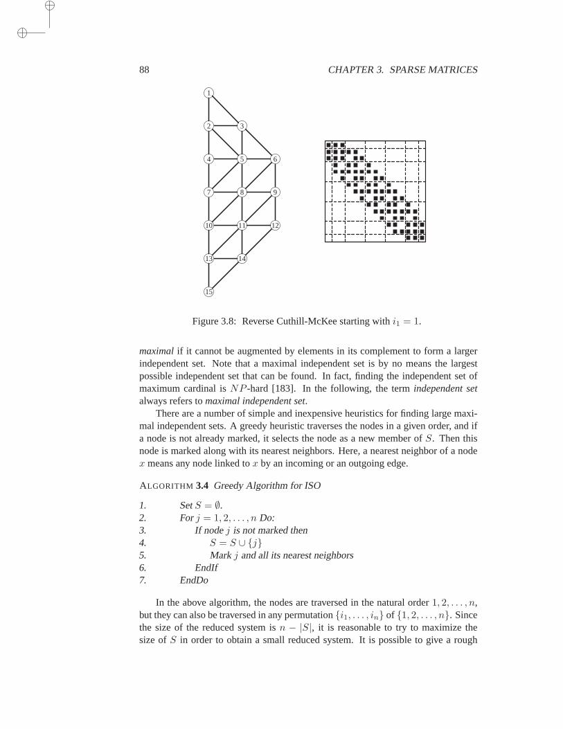
88 CHAPTER 3. SPARSE MATRICES
1
2 3
4 5 6
7 8 9
10 11 12
13 14
15
Figure 3.8: Reverse Cuthill-McKee starting withi1 = 1.
maximalif it cannot be augmented by elements in its complement to form a largerindependent set. Note that a maximal independent set is by no means the largestpossible independent set that can be found. In fact, finding the independent set ofmaximum cardinal isNP -hard [183]. In the following, the termindependent setalways refers tomaximal independent set.
There are a number of simple and inexpensive heuristics for finding largemaxi-mal independent sets. A greedy heuristic traverses the nodes in a givenorder, and ifa node is not already marked, it selects the node as a new member ofS. Then thisnode is marked along with its nearest neighbors. Here, a nearest neighbor of a nodex means any node linked tox by an incoming or an outgoing edge.
ALGORITHM 3.4 Greedy Algorithm for ISO
1. SetS = ∅.2. Forj = 1, 2, . . . , n Do:3. If nodej is not marked then4. S = S ∪ j5. Markj and all its nearest neighbors6. EndIf7. EndDo
In the above algorithm, the nodes are traversed in the natural order1, 2, . . . , n,but they can also be traversed in any permutationi1, . . . , in of 1, 2, . . . , n. Sincethe size of the reduced system isn − |S|, it is reasonable to try to maximize thesize ofS in order to obtain a small reduced system. It is possible to give a rough
3.3. PERMUTATIONS AND REORDERINGS 89
idea of the size ofS. Assume that the maximum degree of each node does notexceedν. Whenever the above algorithm accepts a node as a new member ofS, itpotentially puts all its nearest neighbors, i.e., at mostν nodes, in the complement ofS. Therefore, ifs is the size ofS, the size of its complement,n − s, is such thatn− s ≤ νs, and as a result,
s ≥ n
1 + ν.
This lower bound can be improved slightly by replacingν with the maximum degreeνS of all the vertices that constituteS. This results in the inequality
s ≥ n
1 + νS,
which suggests that it may be a good idea to first visit the nodes with smaller degrees.In fact, this observation leads to a general heuristic regarding a good order of traver-sal. The algorithm can be viewed as follows: Each time a node is visited, removeitand its nearest neighbors from the graph, and then visit a node from theremaininggraph. Continue in the same manner until all nodes are exhausted. Every node that isvisited is a member ofS and its nearest neighbors are members ofS. As result, ifνi
is the degree of the node visited at stepi, adjusted for all the edge deletions resultingfrom the previous visitation steps, then the numberni of nodes that are left at stepisatisfies the relation
ni = ni−1 − νi − 1.
The process adds a new element to the setS at each step and stops whenni = 0.In order to maximize|S|, the number of steps in the procedure must be maximized.The difficulty in the analysis arises from the fact that the degrees are updated at eachstepi because of the removal of the edges associated with the removed nodes. If theprocess is to be lengthened, a rule of thumb would be to visit the nodes that have thesmallest degrees first.
ALGORITHM 3.5 Increasing Degree Traversal for ISO
1. SetS = ∅. Find an orderingi1, . . . , in of the nodes by increasing degree.2. Forj = 1, 2, . . . n, Do:3. If nodeij is not marked then4. S = S ∪ ij5. Mark ij and all its nearest neighbors6. EndIf7. EndDo
A refinement to the above algorithm would be to update the degrees of all nodesinvolved in a removal, and dynamically select the one with the smallest degree asthenext node to be visited. This can be implemented efficiently using a min-heap datastructure. A different heuristic is to attempt to maximize the number of elements inSby a form of local optimization which determines the order of traversal dynamically.In the following, removing a vertex from a graph means deleting the vertex and alledges incident to/from this vertex.
90 CHAPTER 3. SPARSE MATRICES
Example 3.5. The algorithms described in this section were tested on the sameexample used before, namely, the finite element mesh problem of Figure 2.10.Here,all strategies used yield the initial independent set in the matrix itself, which corre-sponds to the nodes of all the previous levels of refinement. This may well beoptimalin this case, i.e., a larger independent set may not exist.
Multicolor orderings. Graph coloring is a familiar problem in computer sciencewhich refers to the process of labeling (coloring) the nodes of a graph insuch a waythat no two adjacent nodes have the same label (color). The goal of graph color-ing is to obtain a colored graph which uses the smallest possible number of colors.However, optimality in the context of numerical linear algebra is a secondaryissueand simple heuristics do provide adequate colorings. Basic methods for obtaining amulticoloring of an arbitrary grid are quite simple. They rely on greedy techniques,a simple version of which is as follows.
ALGORITHM 3.6 Greedy Multicoloring Algorithm
1. Fori = 1, . . . , n Do: setColor(i) = 0.2. Fori = 1, 2, . . . , n Do:3. Set Color(i) = min k > 0 | k 6= Color(j),∀ j ∈ Adj(i))4. EndDo
Line 3 assigns the smallestallowablecolor number to nodei. Allowable means apositive number that is different from the colors of the neighbors of node i. Theprocedure is illustrated in Figure 3.9. The node being colored in the figure isindi-cated by an arrow. It will be assigned color number 3, the smallest positiveintegerdifferent from 1, 2, 4, 5.
In the above algorithm, the order1, 2, . . . , n has been arbitrarily selected fortraversing the nodes and coloring them. Instead, the nodes can be traversed in anyorderi1, i2, . . . , in. If a graph isbipartite, i.e., if it can be colored with twocolors, then the algorithm will find the optimal two-color (Red-Black) ordering forBreadth-Firsttraversals. In addition, if a graph is bipartite, it is easy to show thatthe algorithm will find two colors for any traversal which, at a given step,visits anunmarked node that is adjacent to at least one visited node. In general, the numberof colors needed does not exceed the maximum degree of each node +1.Theseproperties are the subject of Exercises 11 and 10.
Example 3.6. Figure 3.10 illustrates the algorithm for the same example used ear-lier, i.e., the finite element mesh problem of Figure 2.10. The dashed lines separatethe different color sets found. Four colors are found in this example.
Once the colors have been found, the matrix can be permuted to have a blockstructure in which the diagonal blocks are diagonal. Alternatively, the color setsSj = [i
(j)1 , . . ., i(j)nj ] and the permutation array in the algorithms can be used.
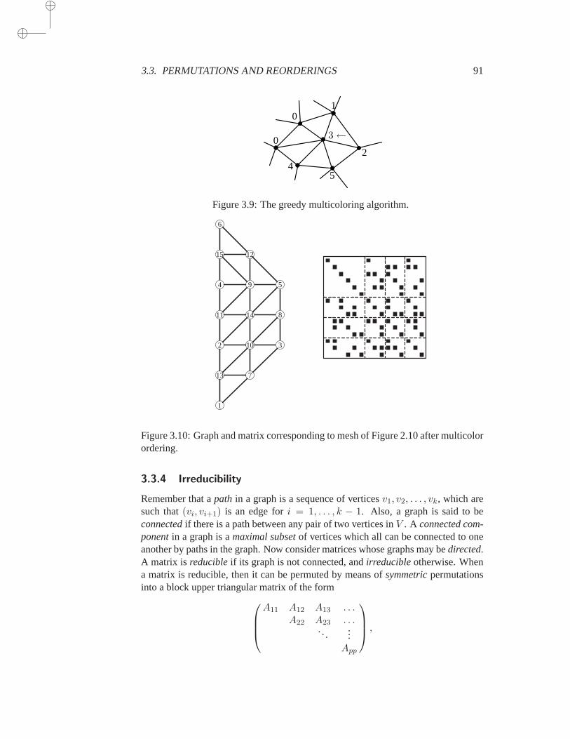
3.3. PERMUTATIONS AND REORDERINGS 91
3←
45
2
10
0
Figure 3.9: The greedy multicoloring algorithm.
1
2 3
4 5
6
7
8
9
10
11
12
13
14
15
Figure 3.10: Graph and matrix corresponding to mesh of Figure 2.10 after multicolorordering.
3.3.4 Irreducibility
Remember that apath in a graph is a sequence of verticesv1, v2, . . . , vk, which aresuch that(vi, vi+1) is an edge fori = 1, . . . , k − 1. Also, a graph is said to beconnectedif there is a path between any pair of two vertices inV . A connected com-ponentin a graph is amaximal subsetof vertices which all can be connected to oneanother by paths in the graph. Now consider matrices whose graphs may bedirected.A matrix is reducibleif its graph is not connected, andirreducibleotherwise. Whena matrix is reducible, then it can be permuted by means ofsymmetricpermutationsinto a block upper triangular matrix of the form
A11 A12 A13 . . .A22 A23 . . .
. .....
App
,
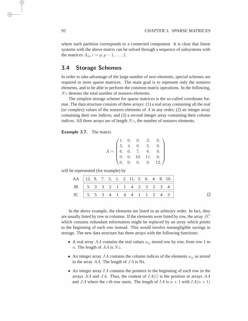
92 CHAPTER 3. SPARSE MATRICES
where each partition corresponds to a connected component. It is clear that linearsystems with the above matrix can be solved through a sequence of subsystems withthe matricesAii, i = p, p− 1, . . . , 1.
3.4 Storage Schemes
In order to take advantage of the large number of zero elements, special schemes arerequired to store sparse matrices. The main goal is to represent only the nonzeroelements, and to be able to perform the common matrix operations. In the following,Nz denotes the total number of nonzero elements.
The simplest storage scheme for sparse matrices is the so-called coordinatefor-mat. The data structure consists of three arrays: (1) a real array containing all the real(or complex) values of the nonzero elements ofA in any order; (2) an integer arraycontaining their row indices; and (3) a second integer array containing their columnindices. All three arrays are of lengthNz, the number of nonzero elements.
Example 3.7. The matrix
A =
1. 0. 0. 2. 0.3. 4. 0. 5. 0.6. 0. 7. 8. 9.0. 0. 10. 11. 0.0. 0. 0. 0. 12.
will be represented (for example) by
AA 12. 9. 7. 5. 1. 2. 11. 3. 6. 4. 8. 10.
JR 5 3 3 2 1 1 4 2 3 2 3 4
JC 5 5 3 4 1 4 4 1 1 2 4 3
In the above example, the elements are listed in an arbitrary order. In fact, theyare usually listed by row or columns. If the elements were listed by row, the arrayJCwhich contains redundant information might be replaced by an array whichpointsto the beginning of each row instead. This would involve nonnegligible savings instorage. The new data structure has three arrays with the following functions:
• A real arrayAA contains the real valuesaij stored row by row, from row 1 ton. The length ofAA isNz.
• An integer arrayJA contains the column indices of the elementsaij as storedin the arrayAA. The length ofJA is Nz.
• An integer arrayIA contains the pointers to the beginning of each row in thearraysAA andJA. Thus, the content ofIA(i) is the position in arraysAAandJA where thei-th row starts. The length ofIA is n + 1 with IA(n + 1)
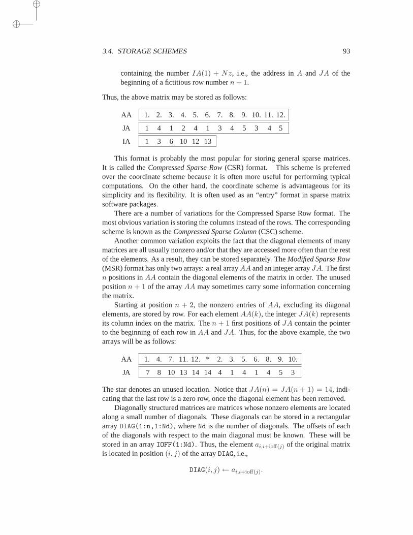
3.4. STORAGE SCHEMES 93
containing the numberIA(1) + Nz, i.e., the address inA and JA of thebeginning of a fictitious row numbern+ 1.
Thus, the above matrix may be stored as follows:
AA 1. 2. 3. 4. 5. 6. 7. 8. 9. 10. 11. 12.
JA 1 4 1 2 4 1 3 4 5 3 4 5
IA 1 3 6 10 12 13
This format is probably the most popular for storing general sparse matrices.It is called theCompressed Sparse Row(CSR) format. This scheme is preferredover the coordinate scheme because it is often more useful for performing typicalcomputations. On the other hand, the coordinate scheme is advantageous for itssimplicity and its flexibility. It is often used as an “entry” format in sparse matrixsoftware packages.
There are a number of variations for the Compressed Sparse Row format.Themost obvious variation is storing the columns instead of the rows. The correspondingscheme is known as theCompressed Sparse Column(CSC) scheme.
Another common variation exploits the fact that the diagonal elements of manymatrices are all usually nonzero and/or that they are accessed more oftenthan the restof the elements. As a result, they can be stored separately. TheModified Sparse Row(MSR) format has only two arrays: a real arrayAA and an integer arrayJA. The firstn positions inAA contain the diagonal elements of the matrix in order. The unusedpositionn + 1 of the arrayAA may sometimes carry some information concerningthe matrix.
Starting at positionn + 2, the nonzero entries ofAA, excluding its diagonalelements, are stored by row. For each elementAA(k), the integerJA(k) representsits column index on the matrix. Then + 1 first positions ofJA contain the pointerto the beginning of each row inAA andJA. Thus, for the above example, the twoarrays will be as follows:
AA 1. 4. 7. 11. 12. * 2. 3. 5. 6. 8. 9. 10.
JA 7 8 10 13 14 14 4 1 4 1 4 5 3
The star denotes an unused location. Notice thatJA(n) = JA(n + 1) = 14, indi-cating that the last row is a zero row, once the diagonal element has been removed.
Diagonally structured matrices are matrices whose nonzero elements are locatedalong a small number of diagonals. These diagonals can be stored in a rectangulararrayDIAG(1:n,1:Nd), whereNd is the number of diagonals. The offsets of eachof the diagonals with respect to the main diagonal must be known. These will bestored in an arrayIOFF(1:Nd). Thus, the elementai,i+ioff(j) of the original matrixis located in position(i, j) of the arrayDIAG, i.e.,
DIAG(i, j)← ai,i+ioff(j).
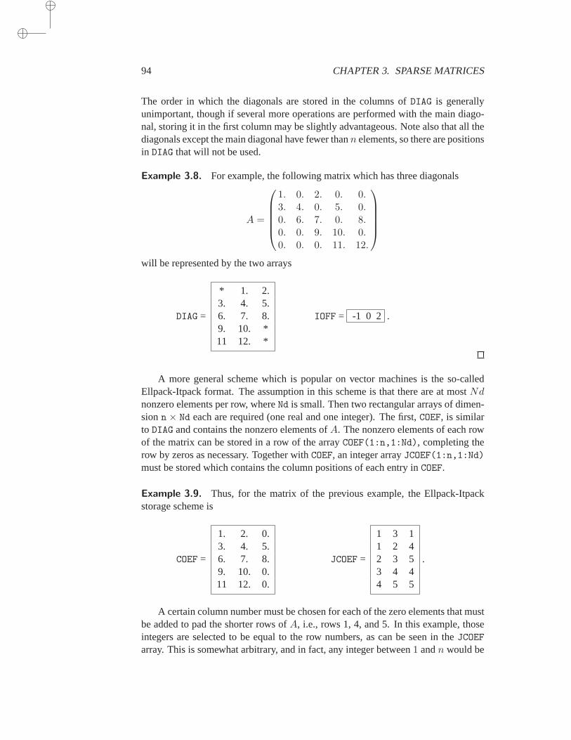
94 CHAPTER 3. SPARSE MATRICES
The order in which the diagonals are stored in the columns ofDIAG is generallyunimportant, though if several more operations are performed with the main diago-nal, storing it in the first column may be slightly advantageous. Note also that allthediagonals except the main diagonal have fewer thann elements, so there are positionsin DIAG that will not be used.
Example 3.8. For example, the following matrix which has three diagonals
A =
1. 0. 2. 0. 0.3. 4. 0. 5. 0.0. 6. 7. 0. 8.0. 0. 9. 10. 0.0. 0. 0. 11. 12.
will be represented by the two arrays
DIAG =
* 1. 2.3. 4. 5.6. 7. 8.9. 10. *11 12. *
IOFF = -1 0 2 .
A more general scheme which is popular on vector machines is the so-calledEllpack-Itpack format. The assumption in this scheme is that there are at mostNdnonzero elements per row, whereNd is small. Then two rectangular arrays of dimen-sionn × Nd each are required (one real and one integer). The first,COEF, is similarto DIAG and contains the nonzero elements ofA. The nonzero elements of each rowof the matrix can be stored in a row of the arrayCOEF(1:n,1:Nd), completing therow by zeros as necessary. Together withCOEF, an integer arrayJCOEF(1:n,1:Nd)must be stored which contains the column positions of each entry inCOEF.
Example 3.9. Thus, for the matrix of the previous example, the Ellpack-Itpackstorage scheme is
COEF =
1. 2. 0.3. 4. 5.6. 7. 8.9. 10. 0.11 12. 0.
JCOEF =
1 3 11 2 42 3 53 4 44 5 5
.
A certain column number must be chosen for each of the zero elements that mustbe added to pad the shorter rows ofA, i.e., rows 1, 4, and 5. In this example, thoseintegers are selected to be equal to the row numbers, as can be seen in theJCOEF
array. This is somewhat arbitrary, and in fact, any integer between1 andn would be
3.5. BASIC SPARSE MATRIX OPERATIONS 95
acceptable. However, there may be good reasons for not inserting the same integerstoo often, e.g. a constant number, for performance considerations.
3.5 Basic Sparse Matrix Operations
The matrix-by-vector product is an important operation which is required inmost ofthe iterative solution algorithms for solving sparse linear systems. This sectionshowshow these can be implemented for a small subset of the storage schemes consideredearlier.
The following FORTRAN 90 segment shows the main loop of the matrix-by-vector operation for matrices stored in the Compressed Sparse Row stored format.
DO I=1, N
K1 = IA(I)
K2 = IA(I+1)-1
Y(I) = DOTPRODUCT(A(K1:K2),X(JA(K1:K2)))
ENDDO
Notice that each iteration of the loop computes a different component of theresulting vector. This is advantageous because each of these components can becomputed independently. If the matrix is stored by columns, then the following codecould be used instead:
DO J=1, N
K1 = IA(J)
K2 = IA(J+1)-1
Y(JA(K1:K2)) = Y(JA(K1:K2))+X(J)*A(K1:K2)
ENDDO
In each iteration of the loop, a multiple of thej-th column is added to the result,which is assumed to have been initially set to zero. Notice now that the outer loopis no longer parallelizable. An alternative to improve parallelization is to try to splitthe vector operation in each inner loop. The inner loop has few operations, in gen-eral, so this is unlikely to be a sound approach. This comparison demonstrates thatdata structures may have to change to improve performance when dealing withhighperformance computers.
Now consider the matrix-by-vector product in diagonal storage.
DO J=1, NDIAG
JOFF = IOFF(J)
DO I=1, N
Y(I) = Y(I) +DIAG(I,J)*X(JOFF+I)
ENDDO
ENDDO
96 CHAPTER 3. SPARSE MATRICES
Here, each of the diagonals is multiplied by the vectorx and the result added tothe vectory. It is again assumed that the vectory has been filled with zeros at thestart of the loop. From the point of view of parallelization and/or vectorization, theabove code is probably the better to use. On the other hand, it is not general enough.
Solving a lower or upper triangular system is another important “kernel” insparse matrix computations. The following segment of code shows a simple rou-tine for solving a unit lower triangular systemLx = y for the CSR storage format.
X(1) = Y(1)
DO I = 2, N
K1 = IAL(I)
K2 = IAL(I+1)-1
X(I)=Y(I)-DOTPRODUCT(AL(K1:K2),X(JAL(K1:K2)))
ENDDO
At each step, the inner product of the current solutionxwith thei-th row is computedand subtracted fromy(i). This gives the value ofx(i). Thedotproduct functioncomputes the dot product of two arbitrary vectorsu(k1:k2) andv(k1:k2). ThevectorAL(K1:K2) is thei-th row of the matrixL in sparse format andX(JAL(K1:K2))is the vector of the components ofX gatheredinto a short vector which is consistentwith the column indices of the elements in the rowAL(K1:K2).
3.6 Sparse Direct Solution Methods
Most direct methods for sparse linear systems perform an LU factorization of theoriginal matrix and try to reduce cost by minimizing fill-ins, i.e., nonzero elementsintroduced during the elimination process in positions which were initially zeros.The data structures employed are rather complicated. The early codes relied heavilyon linked listswhich are convenient for inserting new nonzero elements. Linked-list data structures were dropped in favor of other more dynamic schemes that leavesome initial elbow room in each row for the insertions, and then adjust the structureas more fill-ins are introduced.
A typical sparse direct solution solver for positive definite matrices consists offour phases. First, preordering is applied to reduce fill-in. Two popularmethodsare used: minimum degree ordering and nested-dissection ordering. Second, a sym-bolic factorization is performed. This means that the factorization is processed onlysymbolically, i.e., without numerical values. Third, the numerical factorization, inwhich the actual factorsL andU are formed, is processed. Finally, the forward andbackward triangular sweeps are executed for each different right-hand side. In a codewhere numerical pivoting is necessary, the symbolic phase cannot be separated fromthe numerical factorization.
3.6. SPARSE DIRECT SOLUTION METHODS 97
3.6.1 Minimum degree ordering
The minimum degree (MD) algorithm is perhaps the most popular strategy for min-imizeing fill-in in sparse Gaussian elimination, specifically for SPD matrices. At agiven step of Gaussian elimination, this strategy selects the node with the smallestdegree as the next pivot row. This will tend to reduce fill-in. To be exact,it willminimize (locally) an upper bound for the number of fill-ins that will be introducedat the corrresponding step of Gaussian Elimination.
In contrast with the Cuthill McKee ordering, minimum degree ordering does nothave, nor does it attempt to have, a banded structure. While the algorithm is excellentfor sparse direct solvers, it has been observed that it does not perform as the RCMordering when used in conjunction with preconditioning (Chapter 10).
The Multiple Minimum Degree algorithm is a variation due to Liu [204, 143]which exploits independent sets of pivots at each step. Degrees of nodes adjacentto any vertex in the independent set are updated only after all vertices in the set areprocessed.
3.6.2 Nested Dissection ordering
Nested dissection is used primarily to reduce fill-in in sparse direct solvers for Sym-metric Positive Definite matrices. The technique is easily described with the helpof recursivity and by exploiting the concept of ‘separators’. A setS of vertices in agraph is called a separator if the removal ofS results in the graph being split in twodisjoint subgraphs. For example, each of the intermediate levels in the BFS algorithmis in fact a separator. The nested dissection algorithm can be succinctly described bythe following algorithm
ALGORITHM 3.7 ND(G,nmin)
1. If |V | ≤ nmin2. label nodes ofV3. Else4. Find a separatorS for V5. Label the nodes ofS6. SplitV intoGL,GR by removingS7. ND(GL, nmin)8. ND(GR, nmin)9. End
The labeling of the nodes in Lines 2 and 5, usually proceeds in sequence,so forexample, in Line 5, the nodes ofS are labeled in a certain order, starting from thelast labeled node so far in the procedure. The main step of the ND procedure is toseparate the graph in three parts, two of which have no coupling between each other.The third set has couplings with vertices from both of the first sets and is referred toas a sepator. The key idea is to separate the graph in this way and then repeat the

98 CHAPTER 3. SPARSE MATRICES
process recursively in each subgraph. The nodes of the separatorare numbered last.An illustration is shown in 3.11.
12
43
65
7
Figure 3.11: Nested dissection ordering and corresponding reordered matrix
3.7 Test Problems
For comparison purposes it is important to use a common set of test matrices thatrepresent a wide spectrum of applications. There are two distinct ways of providingsuch data sets. The first approach is to collect sparse matrices in a well-specifiedstandard format from various applications. This approach is used in the Harwell-Boeing collection of test matrices. The second approach is to generate these matriceswith a few sample programs such as those provided in the SPARSKIT library [245].The coming chapters will use examples from these two sources. In particular, fivetest problems will be emphasized for their varying degrees of difficulty.
The SPARSKIT package can generate matrices arising from the discretization ofthe two- or three-dimensional Partial Differential Equations
− ∂
∂x
(
a∂u
∂x
)
− ∂
∂y
(
b∂u
∂y
)
− ∂
∂z
(
c∂u
∂z
)
+∂ (du)
∂x+∂ (eu)
∂y+∂ (fu)
∂z+ gu = h
on rectangular regions with general mixed-type boundary conditions. Inthe testproblems, the regions are the squareΩ = (0, 1)2, or the cubeΩ = (0, 1)3; theDirichlet conditionu = 0 is always used on the boundary. Only the discretized ma-trix is of importance, since the right-hand side will be created artificially. Therefore,the right-hand side,h, is not relevant.

3.7. TEST PROBLEMS 99
a(x, y) =
b(x, y) =
103
-
6
a(x, y) = b(x, y) = 1
14
34
14
34
Figure 3.12: Physical domain and coefficients for Problem 2.
Problem 1: F2DA. In the first test problem which will be labeled F2DA, thedomain is two-dimensional, with
a(x, y) = b(x, y) = 1.0
and
d(x, y) = γ(x+ y), e(x, y) = γ(x− y), f(x, y) = g(x, y) = 0.0, (3.4)
where the constantγ is equal to 10. If the number of points in each direction is 34,then there arenx = ny = 32 interior points in each direction and a matrix of sizen = nx × ny = 322 = 1024 is obtained. In this test example, as well as the otherones described below, the right-hand side is generated as
b = Ae,
in which e = (1, 1, . . . , 1)T . The initial guess is always taken to be a vector ofpseudo-random values.
Problem 2: F2DB. The second test problem is similar to the previous one butinvolves discontinuous coefficient functionsa andb. Here,nx = ny = 32 and thefunctionsd, e, f, g are also defined by (3.4). However, the functionsa andb nowboth take the value 1,000 inside the subsquare of width1
2 centered at (12 ,12 ), and one
elsewhere in the domain, i.e.,
a(x, y) = b(x, y) =
103 if 1
4 < x, y < 34
1 otherwise.
The domain and coefficients for this problem are shown is Figure 3.12.
100 CHAPTER 3. SPARSE MATRICES
Problem 3: F3D. The third test problem is three-dimensional withnx = ny =nz = 16 internal mesh points in each direction leading to a problem of sizen =4096. In this case, we take
a(x, y, z) = b(x, y, z) = c(x, y, z) = 1
d(x, y, z) = γexy, e(x, y, z) = γe−xy,
andf(x, y, z) = g(x, y, z) = 0.0.
The constantγ is taken to be equal to 10.0 as before.The Harwell-Boeing collection is a large data set consisting of test matrices
which have been contributed by researchers and engineers from manydifferent dis-ciplines. These have often been used for test purposes in the literature [108]. Thecollection provides a data structure which constitutes an excellent medium forex-changing matrices. The matrices are stored as ASCII files with a very specific for-mat consisting of a four- or five-line header. Then, the data containing thematrixis stored in CSC format together with any right-hand sides, initial guesses, or exactsolutions when available. The SPARSKIT library also provides routines for readingand generating matrices in this format.
Only one matrix from the collection was selected for testing the algorithms de-scribed in the coming chapters. The matrices in the last two test examples are bothirregularly structured.
Problem 4: ORS The matrix selected from the Harwell-Boeing collection isORSIRR1. This matrix arises from a reservoir engineering problem. Its size isn = 1030 and it has a total ofNz =6,858 nonzero elements. The original prob-lem is based on a21 × 21 × 5 irregular grid. In this case and the next one, thematrices are preprocessed by scaling their rows and columns.
Problem 5: FID This test matrix is extracted from the well known fluid flowsimulation package FIDAP [120]. It is actually the test example number 36 from thispackage and features a two-dimensional Chemical Vapor Deposition in a HorizontalReactor. The matrix has a size ofn = 3079 and hasNz = 53843 nonzero elements.It has a symmetric pattern and few diagonally dominant rows or columns. The rowsand columns are prescaled in the same way as in the previous example. Figure3.13shows the patterns of the matrices ORS and FID.
PROBLEMS
P-3.1 Consider the mesh of a discretized PDE. In which situations is the graph representingthis mesh the same as the adjacency graph of the matrix? Give examples from both FiniteDifference and Finite Element discretizations.
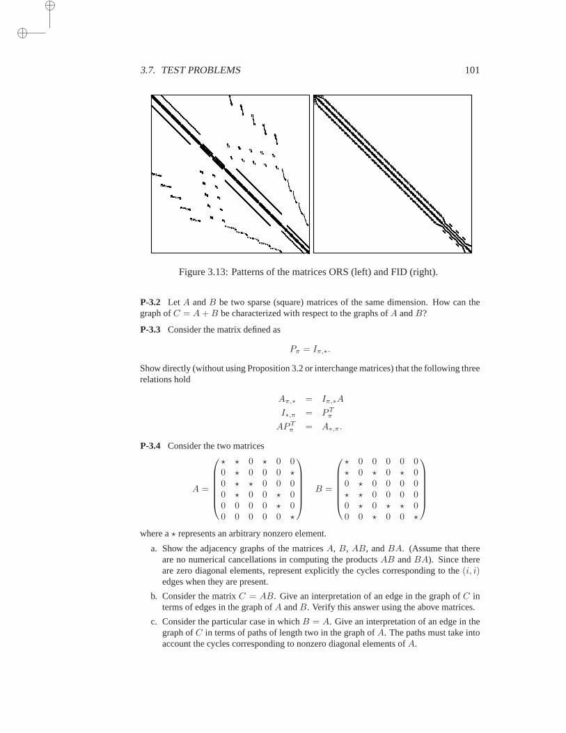
3.7. TEST PROBLEMS 101
Figure 3.13: Patterns of the matrices ORS (left) and FID (right).
P-3.2 Let A andB be two sparse (square) matrices of the same dimension. How can thegraph ofC = A+B be characterized with respect to the graphs ofA andB?
P-3.3 Consider the matrix defined as
Pπ = Iπ,∗.
Show directly (without using Proposition 3.2 or interchange matrices) that the following threerelations hold
Aπ,∗ = Iπ,∗A
I∗,π = PTπ
APTπ = A∗,π.
P-3.4 Consider the two matrices
A =
⋆ ⋆ 0 ⋆ 0 00 ⋆ 0 0 0 ⋆0 ⋆ ⋆ 0 0 00 ⋆ 0 0 ⋆ 00 0 0 0 ⋆ 00 0 0 0 0 ⋆
B =
⋆ 0 0 0 0 0⋆ 0 ⋆ 0 ⋆ 00 ⋆ 0 0 0 0⋆ ⋆ 0 0 0 00 ⋆ 0 ⋆ ⋆ 00 0 ⋆ 0 0 ⋆
where a⋆ represents an arbitrary nonzero element.
a. Show the adjacency graphs of the matricesA, B, AB, andBA. (Assume that thereare no numerical cancellations in computing the productsAB andBA). Since thereare zero diagonal elements, represent explicitly the cycles corresponding to the(i, i)edges when they are present.
b. Consider the matrixC = AB. Give an interpretation of an edge in the graph ofC interms of edges in the graph ofA andB. Verify this answer using the above matrices.
c. Consider the particular case in whichB = A. Give an interpretation of an edge in thegraph ofC in terms of paths of length two in the graph ofA. The paths must take intoaccount the cycles corresponding to nonzero diagonal elements ofA.
102 CHAPTER 3. SPARSE MATRICES
d. Now consider the case whereB = A2. Give an interpretation of an edge in the graphof C = A3 in terms of paths of length three in the graph ofA. Generalize the result toarbitrary powers ofA.
P-3.5 Consider two matricesA andB of dimensionn×n, whose diagonal elements are allnonzeros. LetEX denote the set of edges in the adjacency graph of a matrixX (i.e., the setof pairs(i, j) suchXij 6= 0), then show that
EAB ⊃ EA ∪ EB .
Give extreme examples when|EAB | = n2 while EA ∪ EB is of ordern. What practicalimplications does this have on ways to store products of sparse matrices (Is it better so storethe productAB or the pairsA, B separately? Consider both the computational cost forperforming matrix-vector products and the cost of memory)
P-3.6 Consider a6× 6 matrix which has the pattern
A =
⋆ ⋆ ⋆⋆ ⋆ ⋆ ⋆
⋆ ⋆⋆ ⋆
⋆ ⋆ ⋆ ⋆⋆ ⋆ ⋆
.
a. Show the adjacency graph ofA.
b. Consider the permutationπ = 1, 3, 4, 2, 5, 6. Show the adjacency graph and newpattern for the matrix obtained from a symmetric permutation of A based on the per-mutation arrayπ.
P-3.7 You are given an8 matrix which has the following pattern:
x x xx x x x x
x x x xx x x
x x xx x x x xx x x x
x x x
a. Show the adjacency graph ofA ;
b. Find the Cuthill Mc Kee ordering for the matrix (break tiesby giving priority to thenode with lowest index). Show the graph of the matrix permuted according to theCuthill-Mc Kee ordering.
c. What is the Reverse Cuthill Mc Kee ordering for this case? Show the matrix reorderedaccording to the reverse Cuthill Mc Kee ordering.
d. Find a multicoloring of the graph using the greedy multicolor algorithm. What is theminimum number of colors required for multicoloring the graph?
e. Consider the variation of the Cuthill Mc-Kee ordering in which the first level consistsL0 several vertices instead on only one vertex. Find the Cuthill Mc Kee ordering withthis variant with the starting levelL0 = 1, 8.
3.7. TEST PROBLEMS 103
P-3.8 Consider a matrix which has the pattern
A =
⋆ ⋆ ⋆ ⋆⋆ ⋆ ⋆ ⋆
⋆ ⋆ ⋆ ⋆⋆ ⋆ ⋆ ⋆
⋆ ⋆ ⋆ ⋆⋆ ⋆ ⋆ ⋆
⋆ ⋆ ⋆ ⋆⋆ ⋆ ⋆ ⋆
.
a. Show the adjacency graph ofA. (Place the 8 vertices on a circle.)
b. Consider the permutationπ = 1, 3, 5, 7, 2, 4, 6, 8. Show the adjacency graph andnew pattern for the matrix obtained from a symmetric permutation of A based on thepermutation arrayπ.
c. Show the adjacency graph and new pattern for the matrix obtained from a reverseCuthill-McKee ordering ofA starting with the node 1. (Assume the vertices adjacentto a given vertex are always listed in increasing order in thedata structure that describesthe graph.)
d. Find a multicolor ordering forA (give the vertex labels color 1, followed by those forcolor 2, etc.).
P-3.9 Given a five-point finite difference graph, show that the greedy algorithm will alwaysfind a coloring of the graph with two colors.
P-3.10 Prove that the total number of colors found by the greedy multicoloring algorithmdoes not exceedνmax + 1, whereνmax is the maximum degree of all the vertices of a graph(not counting the cycles(i, i) associated with diagonal elements).
P-3.11 Consider a graph that is bipartite, i.e., 2-colorable. Assume that the vertices of thegraph are colored by a variant of Algorithm (3.6), in which the nodes are traversed in a certainorderi1, i2, . . . , in.
a. Is it true that for any permutationi1, . . . , in the number of colors found will be two?
b. Consider now a permutation satisfying the following property: for eachj at least oneof the nodesi1, i2, . . . , ij−1 is adjacent toij . Show that the algorithm will find a2-coloring of the graph.
c. Among the following traversals indicate which ones satisfy the property of the previousquestion: (1) Breadth-First Search, (2) random traversal,(3) traversal defined byij =any node adjacent toij−1.
P-3.12 Given a matrix that is irreducible and with a symmetric pattern, show that its struc-tural inverse is dense. Structural inverse means the pattern of the inverse, regardless of thevalues, or otherwise stated, is the union of all patterns of the inverses for all possible val-ues. [Hint: Use Cayley Hamilton’s theorem and a well known result on powers of adjacencymatrices mentioned at the end of Section 3.2.1.]
P-3.13 The most economical storage scheme in terms of memory usage is the followingvariation on the coordinate format: Store all nonzero values aij in a real arrayAA[1 : Nz]and the corresponding “linear array address”(i−1)∗n+j in an integer arrayJA[1 : Nz]. Theorder in which these corresponding entries are stored is unimportant as long as they are bothin the same position in their respective arrays. What are the advantages and disadvantages of
104 CHAPTER 3. SPARSE MATRICES
this data structure? Write a short routine for performing a matrix-by-vector product in thisformat.
P-3.14 Write a FORTRAN-90 or C code segment to perform the matrix-by-vector productfor matrices stored in Ellpack-Itpack format.
P-3.15 Write a small subroutine to perform the following operationson a sparse matrix incoordinate format, diagonal format, and CSR format:
a. Count the number of nonzero elements in the main diagonal;
b. Extract the diagonal whose offset isk;
c. Add a nonzero element in position(i, j) of the matrix (this position may initially con-tain a zero or a nonzero element);
d. Add a given diagonal to the matrix. What is the most convenient storage scheme foreach of these operations?
P-3.16 Linked lists is another popular scheme often used for storing sparse matrices. Theseallow to link togetherk data items (e.g., elements of a given row) in a large linear array. Astarting position is given in the array which contains the first element of the set. Then, a linkto the next element in the array is provided from a LINK array.
a. Show how to implement this scheme. A linked list is to be used for each row.
b. What are the main advantages and disadvantages of linked lists?
c. Write an algorithm to perform a matrix-by-vector product in this format.
NOTES AND REFERENCES. Two good references on sparse matrix computations are the book byGeorge and Liu [144] and the more recent volume by Duff, Erisman, and Reid [107]. These are gearedtoward direct solution methods and the first specializes in symmetric positive definite problems. Alsoof interest are [221] and [227] and the early survey by Duff [106].
Sparse matrix techniques have traditionally been associated with direct solution methods. Thishas changed in the last decade because of the increased need to solve three-dimensional problems. TheSPARSKIT library, a package for sparse matrix computations [245] is available from the author at:http://www.cs.umn.edu/ saad/software .Another available software package which emphasizes object-oriented design with the goal of hidingcomplex data structures from users is PETSc [24].
The idea of the greedy multicoloring algorithm is known in Finite Element techniques (to colorelements); see, e.g., Benantar and Flaherty [31]. Wu [319] presents the greedy algorithm for multicol-oring vertices and uses it for SOR type iterations, see also [248]. The effect of multicoloring has beenextensively studied by Adams [2, 3] and Poole and Ortega [228]. Interesting results regarding multi-coloring in the context of finite elements based on quad-tree structures have been obtained by Benantarand Flaherty [31] who show, in particular, that with this structure a maximumof six colors is required.
Chapter 4
BASIC ITERATIVE METHODS
The first iterative methods used for solving large linear systems were based on relaxation of the
coordinates. Beginning with a given approximate solution, these methods modify the compo-
nents of the approximation, one or a few at a time and in a certain order, until convergence is
reached. Each of these modifications, called relaxation steps, is aimed at annihilating one or a
few components of the residual vector. Now, these techniques are rarely used separately. How-
ever, when combined with the more efficient methods described in later chapters, they can be
quite successful. Moreover, there are a few application areas where variations of these methods
are still quite popular.
4.1 Jacobi, Gauss-Seidel, and SOR
This chapter begins by reviewing the basic iterative methods for solving linear sys-tems. Given ann× n real matrixA and a realn-vectorb, the problem considered is:Findx belonging toRn such that
Ax = b (4.1)
Equation (4.1) is alinear system, A is the coefficient matrix, b is the right-handside vector, andx is the vector of unknowns. Most of the methods covered inthis chapter involve passing from one iterate to the next by modifying one or afewcomponents of an approximate vector solution at a time. This is natural since thereare simple criteria when modifying a component in order to improve an iterate. Oneexample is to annihilate some component(s) of the residual vectorb − Ax. Theconvergence of these methods is rarely guaranteed for all matrices, buta large body oftheory exists for the case where the coefficient matrix arises from the finitedifferencediscretization of Elliptic Partial Differential Equations.
We begin with the decomposition
A = D − E − F, (4.2)
105
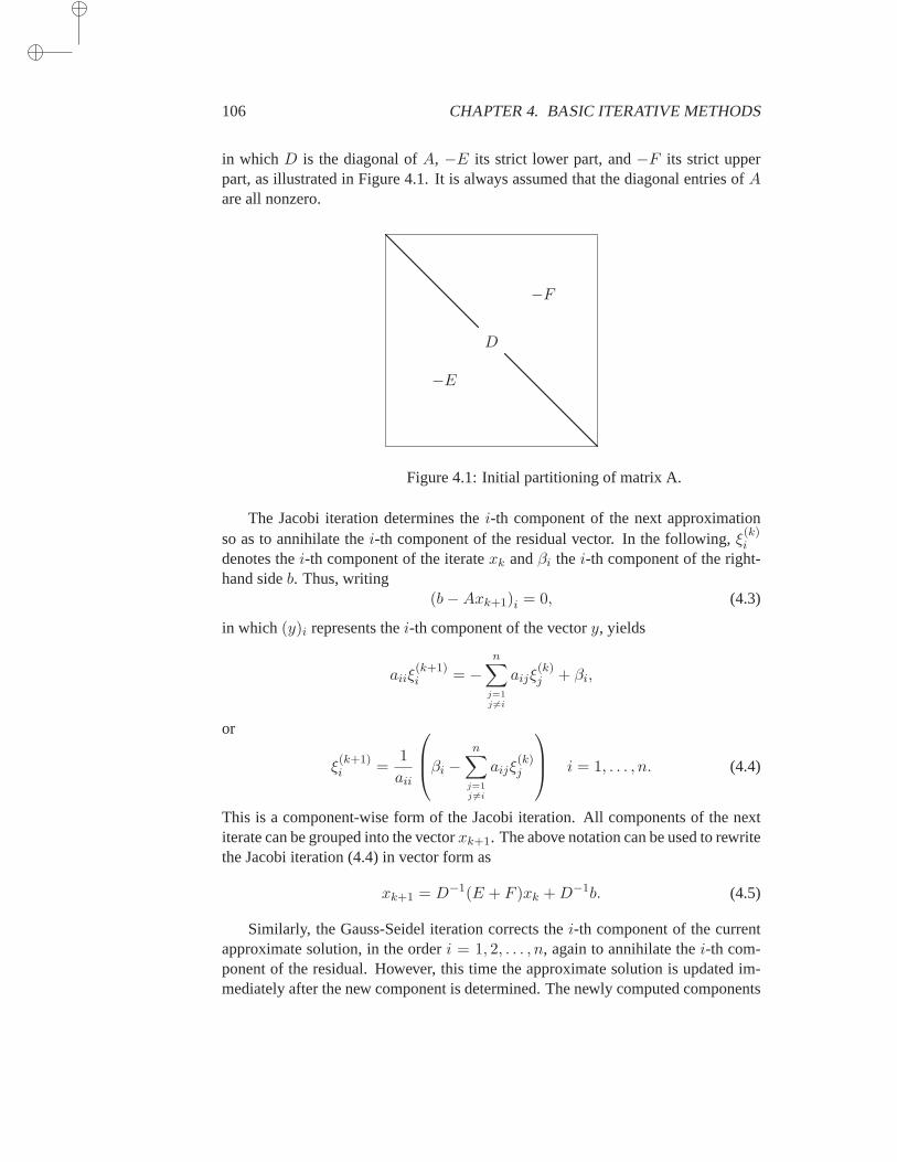
106 CHAPTER 4. BASIC ITERATIVE METHODS
in whichD is the diagonal ofA, −E its strict lower part, and−F its strict upperpart, as illustrated in Figure 4.1. It is always assumed that the diagonal entries ofAare all nonzero.
D
−F
−E
Figure 4.1: Initial partitioning of matrix A.
The Jacobi iteration determines thei-th component of the next approximationso as to annihilate thei-th component of the residual vector. In the following,ξ
(k)i
denotes thei-th component of the iteratexk andβi the i-th component of the right-hand sideb. Thus, writing
(b−Axk+1)i = 0, (4.3)
in which (y)i represents thei-th component of the vectory, yields
aiiξ(k+1)i = −
n∑
j=1j 6=i
aijξ(k)j + βi,
or
ξ(k+1)i =
1
aii
βi −
n∑
j=1j 6=i
aijξ(k)j
i = 1, . . . , n. (4.4)
This is a component-wise form of the Jacobi iteration. All components of the nextiterate can be grouped into the vectorxk+1. The above notation can be used to rewritethe Jacobi iteration (4.4) in vector form as
xk+1 = D−1(E + F )xk +D−1b. (4.5)
Similarly, the Gauss-Seidel iteration corrects thei-th component of the currentapproximate solution, in the orderi = 1, 2, . . . , n, again to annihilate thei-th com-ponent of the residual. However, this time the approximate solution is updated im-mediately after the new component is determined. The newly computed components
4.1. JACOBI, GAUSS-SEIDEL, AND SOR 107
ξ(k)i , i = 1, 2, . . . , n can be changed within a working vector which is redefined at
each relaxation step. Thus, since the order isi = 1, 2, . . ., the result at thei-th step is
βi −i−1∑
j=1
aijξ(k+1)j − aiiξ
(k+1)i −
n∑
j=i+1
aijξ(k)j = 0, (4.6)
which leads to the iteration,
ξ(k+1)i =
1
aii
−i−1∑
j=1
aijξ(k+1)j −
n∑
j=i+1
aijξ(k)j + βi
, i = 1, . . . , n. (4.7)
The defining equation (4.6) can be written as
b+ Exk+1 −Dxk+1 + Fxk = 0,
which leads immediately to the vector form of the Gauss-Seidel iteration
xk+1 = (D − E)−1Fxk + (D − E)−1b. (4.8)
Computing the new approximation in (4.5) requires multiplying by the inverseof the diagonal matrixD. In (4.8) a triangular system must be solved withD − E,the lower triangular part ofA. Thus, the new approximation in a Gauss-Seidel stepcan be determined either by solving a triangular system with the matrixD − E orfrom the relation (4.7).
A backwardGauss-Seidel iteration can also be defined as
(D − F )xk+1 = Exk + b, (4.9)
which is equivalent to making the coordinate corrections in the ordern, n−1, . . . , 1.A Symmetric Gauss-Seidel Iteration consists of a forward sweep followed by a back-ward sweep.
The Jacobi and the Gauss-Seidel iterations are both of the form
Mxk+1 = Nxk + b = (M −A)xk + b, (4.10)
in whichA = M −N (4.11)
is asplitting of A, with M = D for Jacobi,M = D − E for forward Gauss-Seidel,andM = D − F for backward Gauss-Seidel. An iterative method of the form(4.10) can be defined for any splitting of the form (4.11) whereM is nonsingular.Overrelaxationis based on the splitting
ωA = (D − ωE)− (ωF + (1− ω)D),
and the correspondingSuccessive Over Relaxation(SOR) method is given by therecursion
(D − ωE)xk+1 = [ωF + (1− ω)D]xk + ωb. (4.12)
108 CHAPTER 4. BASIC ITERATIVE METHODS
The above iteration corresponds to the relaxation sequence
ξ(k+1)i = ωξGS
i + (1− ω)ξ(k)i , i = 1, 2, . . . , n,
in whichξGSi is defined by the expression in the right-hand side of (4.7). A backward
SOR sweep can be defined analogously to the backward Gauss-Seidel sweep (4.9).A Symmetric SOR (SSOR) step consists of the SOR step (4.12) followed by a
backward SOR step,
(D − ωE)xk+1/2 = [ωF + (1− ω)D]xk + ωb
(D − ωF )xk+1 = [ωE + (1− ω)D]xk+1/2 + ωb
This gives the recurrencexk+1 = Gωxk + fω,
where
Gω = (D − ωF )−1(ωE + (1− ω)D) ×(D − ωE)−1(ωF + (1− ω)D), (4.13)
fω = ω(D − ωF )−1(I + [ωE + (1− ω)D](D − ωE)−1
)b. (4.14)
Observing that
[ωE + (1− ω)D](D − ωE)−1 = [−(D − ωE) + (2− ω)D](D − ωE)−1
= −I + (2− ω)D(D − ωE)−1,
fω can be rewritten as
fω = ω(2− ω) (D − ωF )−1D(D − ωE)−1b.
4.1.1 Block Relaxation Schemes
Block relaxation schemes are generalizations of the “point” relaxation schemes de-scribed above. They update a whole set of components at each time, typically asubvector of the solution vector, instead of only one component. The matrixA andthe right-hand side and solution vectors are partitioned as follows:
A =
A11 A12 A13 · · · A1p
A21 A22 A23 · · · A2p
A31 A32 A33 · · · A3p...
......
.. ....
Ap1 Ap2 · · · · · · App
, x =
ξ1ξ2ξ3...ξp
, b =
β1
β2
β3...βp
, (4.15)
in which the partitionings ofb andx into subvectorsβi and ξi are identical andcompatible with the partitioning ofA. Thus, for any vectorx partitioned as in (4.15),
(Ax)i =
p∑
j=1
Aijξj ,
4.1. JACOBI, GAUSS-SEIDEL, AND SOR 109
in which (y)i denotes thei-th component of the vectori according to the abovepartitioning. The diagonal blocks inA are square and assumed nonsingular.
Now define, similarly to the scalar case, the splitting
A = D − E − F
with
D =
A11
A22.. .
App
, (4.16)
E = −
OA21 O
......
. ..Ap1 Ap2 · · · O
, F = −
O A12 · · · A1p
O · · · A2p. . .
...O
.
With these definitions, it is easy to generalize the previous three iterative proceduresdefined earlier, namely, Jacobi, Gauss-Seidel, and SOR. For example, the block Ja-cobi iteration is now defined as a technique in which the new subvectorsξ
(k)i are all
replaced according to
Aiiξ(k+1)i = ((E + F )xk)i + βi
or,ξ(k+1)i = A−1
ii ((E + F )xk)i +A−1ii βi, i = 1, . . . , p,
which leads to the same equation as before,
xk+1 = D−1(E + F )xk +D−1b,
except that the meanings ofD,E, andF have changed to their block analogues.With finite difference approximations of PDEs, it is standard to block the vari-
ables and the matrix by partitioning along whole lines of the mesh. For example, forthe two-dimensional mesh illustrated in Figure 2.5, this partitioning is
ξ1 =
u11
u12
u13
u14
u15
, ξ2 =
u21
u22
u23
u24
u25
, ξ3 =
u31
u32
u33
u34
u35
.
This corresponds to the mesh 2.5 of Chapter 2, whose associated matrix pattern isshown in Figure 2.6. A relaxation can also be defined along the vertical insteadof the horizontal lines. Techniques of this type are often known asline relaxationtechniques.
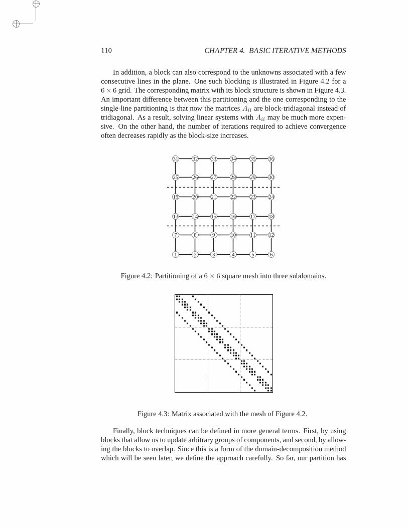
110 CHAPTER 4. BASIC ITERATIVE METHODS
In addition, a block can also correspond to the unknowns associated with afewconsecutive lines in the plane. One such blocking is illustrated in Figure 4.2 for a6× 6 grid. The corresponding matrix with its block structure is shown in Figure 4.3.An important difference between this partitioning and the one corresponding to thesingle-line partitioning is that now the matricesAii are block-tridiagonal instead oftridiagonal. As a result, solving linear systems withAii may be much more expen-sive. On the other hand, the number of iterations required to achieve convergenceoften decreases rapidly as the block-size increases.
1 2 3 4 5 6
7 8 9 10 11 12
13 14 15 16 17 18
19 20 21 22 23 24
25 26 27 28 29 30
31 32 33 34 35 36
Figure 4.2: Partitioning of a6× 6 square mesh into three subdomains.
Figure 4.3: Matrix associated with the mesh of Figure 4.2.
Finally, block techniques can be defined in more general terms. First, by usingblocks that allow us to update arbitrary groups of components, and second, by allow-ing the blocks to overlap. Since this is a form of the domain-decomposition methodwhich will be seen later, we define the approach carefully. So far, our partition has
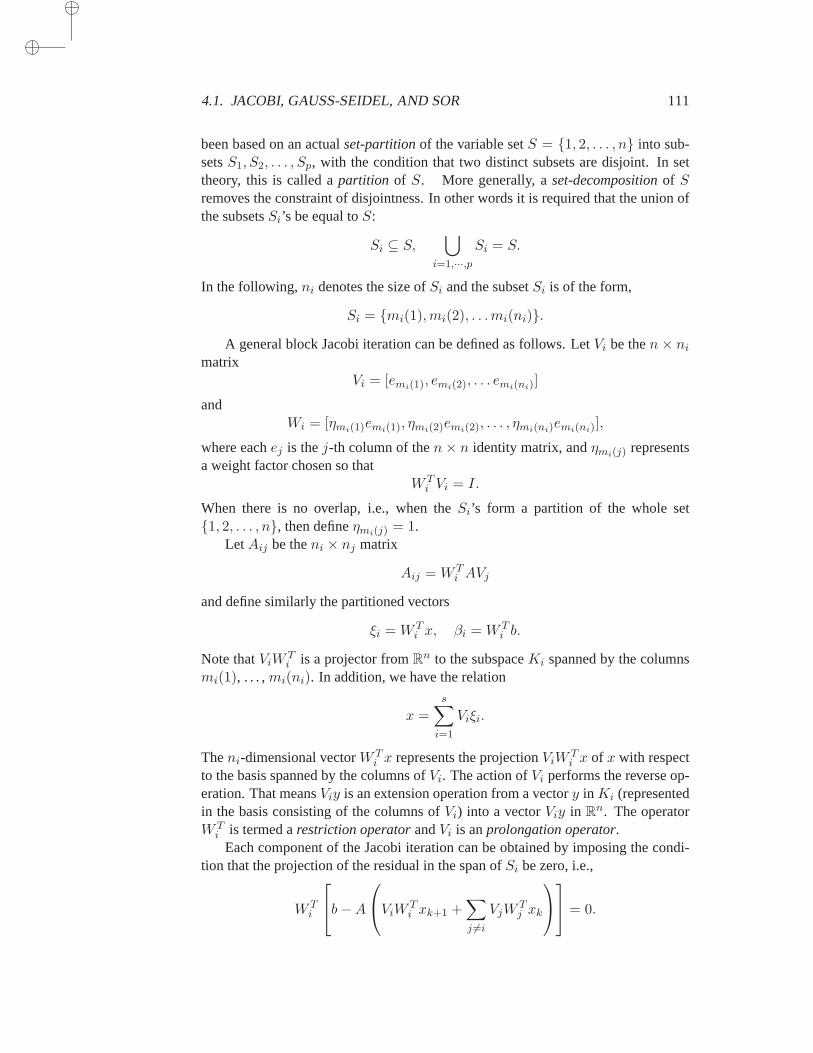
4.1. JACOBI, GAUSS-SEIDEL, AND SOR 111
been based on an actualset-partitionof the variable setS = 1, 2, . . . , n into sub-setsS1, S2, . . . , Sp, with the condition that two distinct subsets are disjoint. In settheory, this is called apartition of S. More generally, aset-decompositionof Sremoves the constraint of disjointness. In other words it is required that the union ofthe subsetsSi’s be equal toS:
Si ⊆ S,⋃
i=1,···,pSi = S.
In the following,ni denotes the size ofSi and the subsetSi is of the form,
Si = mi(1),mi(2), . . .mi(ni).
A general block Jacobi iteration can be defined as follows. LetVi be then× ni
matrixVi = [emi(1), emi(2), . . . emi(ni)]
andWi = [ηmi(1)emi(1), ηmi(2)emi(2), . . . , ηmi(ni)emi(ni)],
where eachej is thej-th column of then× n identity matrix, andηmi(j) representsa weight factor chosen so that
W Ti Vi = I.
When there is no overlap, i.e., when theSi’s form a partition of the whole set1, 2, . . . , n, then defineηmi(j) = 1.
LetAij be theni × nj matrix
Aij = W Ti AVj
and define similarly the partitioned vectors
ξi = W Ti x, βi = W T
i b.
Note thatViWTi is a projector fromR
n to the subspaceKi spanned by the columnsmi(1), . . . ,mi(ni). In addition, we have the relation
x =
s∑
i=1
Viξi.
Theni-dimensional vectorW Ti x represents the projectionViW
Ti x of x with respect
to the basis spanned by the columns ofVi. The action ofVi performs the reverse op-eration. That meansViy is an extension operation from a vectory in Ki (representedin the basis consisting of the columns ofVi) into a vectorViy in R
n. The operatorW T
i is termed arestriction operatorandVi is anprolongation operator.Each component of the Jacobi iteration can be obtained by imposing the condi-
tion that the projection of the residual in the span ofSi be zero, i.e.,
W Ti
b−A
ViWTi xk+1 +
∑
j 6=i
VjWTj xk
= 0.
112 CHAPTER 4. BASIC ITERATIVE METHODS
Remember thatξj = W Tj x, which can be rewritten as
ξ(k+1)i = ξ
(k)i +A−1
ii WTi (b−Axk). (4.17)
This leads to the following algorithm:
ALGORITHM 4.1 General Block Jacobi Iteration
1. Fork = 0, 1, . . . , until convergence Do:2. Fori = 1, 2, . . . , p Do:3. SolveAiiδi = W T
i (b−Axk)4. Setxk+1 := xk + Viδi5. EndDo6. EndDo
As was the case with the scalar algorithms, there is only a slight difference be-tween the Jacobi and Gauss-Seidel iterations. Gauss-Seidel immediately updates thecomponent to be corrected at stepi, and uses the updated approximate solution tocompute the residual vector needed to correct the next component. However, the Ja-cobi iteration uses the same previous approximationxk for this purpose. Therefore,the block Gauss-Seidel iteration can be defined algorithmically as follows:
ALGORITHM 4.2 General Block Gauss-Seidel Iteration
1. Until convergence Do:2. Fori = 1, 2, . . . , p Do:3. SolveAiiδi = W T
i (b−Ax)4. Setx := x+ Viδi5. EndDo6. EndDo
From the point of view of storage, Gauss-Seidel is more economical because the newapproximation can be overwritten over the same vector. Also, it typically convergesfaster. On the other hand, the Jacobi iteration has some appeal on parallel computerssince the secondDo loop, corresponding to thep different blocks, can be executed inparallel. Although the point Jacobi algorithm by itself is rarely a successful techniquefor real-life problems, its block Jacobi variant, when using large enoughoverlappingblocks, can be quite attractive especially in a parallel computing environment.
4.1.2 Iteration Matrices and Preconditioning
The Jacobi and Gauss-Seidel iterations are of the form
xk+1 = Gxk + f, (4.18)
in which
GJA(A) = I −D−1A, (4.19)
GGS(A) = I − (D − E)−1A, (4.20)

4.1. JACOBI, GAUSS-SEIDEL, AND SOR 113
for the Jacobi and Gauss-Seidel iterations, respectively. Moreover, given the matrixsplitting
A = M −N, (4.21)
whereA is associated with the linear system (4.1), alinear fixed-point iterationcanbe defined by the recurrence
xk+1 = M−1Nxk +M−1b, (4.22)
which has the form (4.18) with
G = M−1N = M−1(M −A) = I −M−1A, f = M−1b. (4.23)
For example, for the Jacobi iteration,M = D,N = D − A, while for the Gauss-Seidel iteration,M = D − E,N = M −A = F .
The iterationxk+1 = Gxk + f can be viewed as a technique for solving thesystem
(I −G)x = f.
SinceG has the formG = I −M−1A, this system can be rewritten as
M−1Ax = M−1b.
The above system which has the same solution as the original system is called apre-conditioned systemandM is thepreconditioning matrixor preconditioner. In otherwords,a relaxation scheme is equivalent to a fixed-point iteration on a precondi-tioned system.
For example, for the Jacobi, Gauss-Seidel, SOR, and SSOR iterations, thesepreconditioning matrices are, respectively,
MJA = D, (4.24)
MGS = D − E, (4.25)
MSOR =1
ω(D − ωE), (4.26)
MSSOR =1
ω(2− ω)(D − ωE)D−1(D − ωF ). (4.27)
Thus, the Jacobi preconditioner is simply the diagonal ofA, while the Gauss-Seidelpreconditioner is the lower triangular part ofA. The constant coefficients in front ofthe matricesMSOR andMSSOR only have the effect of scaling the equations of thepreconditioned system uniformly. Therefore, they are unimportant in the precondi-tioning context.
Note that the “preconditioned” system may be a full system. Indeed, there isno reason whyM−1 should be a sparse matrix (even thoughM may be sparse),since the inverse of a sparse matrix is not necessarily sparse. This limits the numberof techniques that can be applied to solve the preconditioned system. Most oftheiterative techniques used only require matrix-by-vector products. In thiscase, to
114 CHAPTER 4. BASIC ITERATIVE METHODS
computew = M−1Av for a given vectorv, first computer = Av and then solve thesystemMw = r:
r = Av,
w = M−1r.
In some cases, it may be advantageous to exploit the splittingA = M − N andcomputew = M−1Av asw = (I −M−1N)v by the procedure
r = Nv,
w = M−1r,
w := v − w.
The matrixN may be sparser thanA and the matrix-by-vector productNv maybe less expensive than the productAv. A number of similar but somewhat morecomplex ideas have been exploited in the context of preconditioned iterativemethods.A few of these will be examined in Chapter 9.
4.2 Convergence
All the methods seen in the previous section define a sequence of iterates ofthe form
xk+1 = Gxk + f, (4.28)
in whichG is a certainiteration matrix. The questions addressed in this section are:(a) if the iteration converges, then is the limit indeed a solution of the original system?(b) under which conditions does the iteration converge? (c) when the iteration doesconverge, how fast is it?
If the above iteration converges, its limitx satisfies
x = Gx+ f. (4.29)
In the case where the above iteration arises from the splittingA = M −N , it is easyto see that the solutionx to the above system is identical to that of the original systemAx = b. Indeed, in this case the sequence (4.28) has the form
xk+1 = M−1Nxk +M−1b
and its limit satisfiesMx = Nx+ b,
orAx = b. This answers question (a). Next, we focus on the other two questions.
4.2. CONVERGENCE 115
4.2.1 General Convergence Result
If I −G is nonsingular then there is a solutionx∗ to the equation (4.29). Subtracting(4.29) from (4.28) yields
xk+1 − x∗ = G(xk − x∗) = · · · = Gk+1(x0 − x∗). (4.30)
Standard results seen in Chapter 1 imply that if the spectral radius of the iterationmatrixG is less than unity, thenxk − x∗ converges to zero and the iteration (4.28)converges toward the solution defined by (4.29). Conversely, the relation
xk+1 − xk = G(xk − xk−1) = · · · = Gk(f − (I −G)x0).
shows that if the iteration converges foranyx0 andf thenGkv converges to zero forany vectorv. As a result,ρ(G) must be less than unity and the following theorem isproved:
Theorem 4.1 LetG be a square matrix such thatρ(G) < 1. ThenI −G is nonsin-gular and the iteration (4.28) converges for anyf andx0. Conversely, if the iteration(4.28) converges for for anyf andx0, thenρ(G) < 1.
Since it is expensive to compute the spectral radius of a matrix, sufficient conditionsthat guarantee convergence can be useful in practice. One such sufficient conditioncould be obtained by utilizing the inequality,ρ(G) ≤ ‖G‖, for any matrix norm.
Corollary 4.2 LetG be a square matrix such that‖G‖ < 1 for some matrix norm‖.‖. ThenI − G is nonsingular and the iteration (4.28) converges for any initialvectorx0.
Apart from knowing that the sequence (4.28) converges, it is also desirable toknowhow fastit converges. The errordk = xk − x∗ at stepk satisfies
dk = Gkd0.
The matrixG can be expressed in the Jordan canonical form asG = XJX−1.Assume for simplicity that there is only one eigenvalue ofG of largest modulus andcall it λ. Then
dk = λkX
(J
λ
)k
X−1d0.
A careful look at the powers of the matrixJ/λ shows that all its blocks, except theblock associated with the eigenvalueλ, converge to zero ask tends to infinity. Letthis Jordan block be of sizep and of the form
Jλ = λI + E,
whereE is nilpotent of indexp, i.e.,Ep = 0. Then, fork ≥ p,
Jkλ = (λI + E)k = λk(I + λ−1E)k = λk
(p−1∑
i=0
λ−i
(k
i
)
Ei
)
.
116 CHAPTER 4. BASIC ITERATIVE METHODS
If k is large enough, then for anyλ the dominant term in the above sum is the lastterm, i.e.,
Jkλ ≈ λk−p+1
(k
p− 1
)
Ep−1.
Thus, the norm ofdk = Gkd0 has the asymptotical form
‖dk‖ ≈ C × |λk−p+1|(
k
p− 1
)
,
whereC is some constant. Theconvergence factorof a sequence is the limit
ρ = limk→∞
(‖dk‖‖d0‖
)1/k
.
It follows from the above analysis thatρ = ρ(G). The convergence rateτ is the(natural) logarithm of the inverse of the convergence factor
τ = − ln ρ.
The above definition depends on the initial vectorx0, so it may be termed aspecificconvergence factor. Ageneralconvergence factor can also be defined by
φ = limk→∞
(
maxx0∈Rn
‖dk‖‖d0‖
)1/k
.
This factor satisfies
φ = limk→∞
(
maxd0∈Rn
‖Gkd0‖‖d0‖
)1/k
= limk→∞
(
‖Gk‖)1/k
= ρ(G).
Thus, the global asymptotic convergence factor is equal to the spectral radius ofthe iteration matrixG. Thegeneralconvergence rate differs from thespecificrateonly when the initial error does not have any components in the invariant subspaceassociated with the dominant eigenvalue. Since it is hard to know this informationinadvance, thegeneralconvergence factor is more useful in practice.
Example 4.1. Consider the simple example ofRichardson’s Iteration,
xk+1 = xk + α (b−Axk) , (4.31)
whereα is a nonnegative scalar. This iteration can be rewritten as
xk+1 = (I − αA)xk + αb. (4.32)
Thus, the iteration matrix isGα = I −αA and the convergence factor isρ(I −αA).Assume that the eigenvaluesλi, i = 1, . . . , n, are all real and such that,
λmin ≤ λi ≤ λmax.
4.2. CONVERGENCE 117
Then, the eigenvaluesµi of Gα are such that
1− αλmax ≤ µi ≤ 1− αλmin.
In particular, ifλmin < 0 andλmax > 0, at least one eigenvalue is> 1, and soρ(Gα) > 1 for anyα. In this case the method will always diverge for some initialguess. Let us assume that all eigenvalues are positive, i.e.,λmin > 0. Then, thefollowing conditions must be satisfied in order for the method to converge:
1− αλmin < 1,
1− αλmax > −1.
The first condition implies thatα > 0, while the second requires thatα ≤ 2/λmax.In other words, the method converges for any scalarα which satisfies
0 < α <2
λmax.
The next question is: What is the best valueαopt for the parameterα, i.e., the valueof α which minimizesρ(Gα)? The spectral radius ofGα is
ρ(Gα) = max|1− αλmin|, |1− αλmax|.
This function ofα is depicted in Figure 4.4. As the curve shows, the best possibleαis reached at the point where the curve|1 − λmaxα| with positive slope crosses thecurve|1− λminα| with negative slope, i.e., when
−1 + λmaxα = 1− λminα.
1λmin
1λmax
αopt
|1− λminα||1− λmaxα|
α
1
Figure 4.4: The curveρ(Gα) as a function ofα.
This gives
αopt =2
λmin + λmax. (4.33)
118 CHAPTER 4. BASIC ITERATIVE METHODS
Replacing this in one of the two curves gives the corresponding optimal spectralradius
ρopt =λmax − λmin
λmax + λmin.
This expression shows the difficulty with the presence of small and large eigenvalues.The convergence rate can be extremely small for realistic problems. In addition, toachieve good convergence, eigenvalue estimates are required in orderto obtain theoptimal or a near-optimalα, and this may cause difficulties. Finally, sinceλmax canbe very large, the curveρ(Gα) can be extremely sensitive near the optimal valueof α. These observations are common to many iterative methods that depend on anacceleration parameter.
4.2.2 Regular Splittings
Definition 4.3 LetA,M,N be three given matrices satisfyingA = M − N . Thepair of matricesM,N is a regular splitting ofA, if M is nonsingular andM−1 andN are nonnegative.
With a regular splitting, we associate the iteration
xk+1 = M−1Nxk +M−1b. (4.34)
The question asked is: Under which conditions does such an iteration converge? Thefollowing result, which generalizes Theorem 1.29, gives the answer.
Theorem 4.4 LetM,N be a regular splitting of a matrixA. Thenρ(M−1N) < 1 ifand only ifA is nonsingular andA−1 is nonnegative.
Proof. DefineG = M−1N . From the fact thatρ(G) < 1, and the relation
A = M(I −G) (4.35)
it follows thatA is nonsingular. The assumptions of Theorem 1.29 are satisfied forthe matrixG sinceG = M−1N is nonnegative andρ(G) < 1. Therefore,(I−G)−1
is nonnegative as isA−1 = (I −G)−1M−1.To prove the sufficient condition, assume thatA is nonsingular and that its inverse
is nonnegative. SinceA andM are nonsingular, the relation (4.35) shows again thatI −G is nonsingular and in addition,
A−1N =(M(I −M−1N)
)−1N
= (I −M−1N)−1M−1N
= (I −G)−1G. (4.36)
Clearly, G = M−1N is nonnegative by the assumptions, and as a result of thePerron-Frobenius theorem, there is a nonnegative eigenvectorx associated withρ(G)which is an eigenvalue, such that
Gx = ρ(G)x.
4.2. CONVERGENCE 119
From this and by virtue of (4.36), it follows that
A−1Nx =ρ(G)
1− ρ(G)x.
Sincex andA−1N are nonnegative, this shows that
ρ(G)
1− ρ(G)≥ 0
and this can be true only when0 ≤ ρ(G) ≤ 1. SinceI − G is nonsingular, thenρ(G) 6= 1, which implies thatρ(G) < 1.
This theorem establishes that the iteration (4.34) always converges, ifM,N is aregular splitting andA is an M-matrix.
4.2.3 Diagonally Dominant Matrices
We begin with a few standard definitions.
Definition 4.5 A matrixA is
• (weakly) diagonally dominant if
|ajj | ≥i=n∑
i=1i6=j
|aij |, j = 1, . . . , n.
• strictly diagonally dominant if
|ajj | >i=n∑
i=1i6=j
|aij |, j = 1, . . . , n.
• irreducibly diagonally dominant ifA is irreducible, and
|ajj | ≥i=n∑
i=1i6=j
|aij |, j = 1, . . . , n.
with strict inequality for at least onej.
Often the term diagonally dominant is used instead ofweaklydiagonally dominant.Diagonal dominance is related to an important result in Numerical Linear Alge-
bra known as Gershgorin’s theorem. This theorem allows rough locationsfor all theeigenvalues ofA to be determined. In some situations, it is desirable to determinethese locations in the complex plane by directly exploiting some knowledge of theentries of the matrixA. The simplest such result is the bound
|λi| ≤ ‖A‖for any matrix norm. Gershgorin’s theorem provides a more precise localizationresult.
120 CHAPTER 4. BASIC ITERATIVE METHODS
Theorem 4.6 (Gershgorin) Any eigenvalueλ of a matrixA is located in one of theclosed discs of the complex plane centered ataii and having the radius
ρi =
j=n∑
j=1j 6=i
|aij |.
In other words,
∀ λ ∈ σ(A), ∃ i such that |λ− aii| ≤j=n∑
j=1j 6=i
|aij |. (4.37)
Proof. Let x be an eigenvector associated with an eigenvalueλ, and letm be theindex of the component of largest modulus inx. Scalex so that|ξm| = 1, and|ξi| ≤ 1, for i 6= m. Sincex is an eigenvector, then
(λ− amm)ξm = −n∑
j=1j 6=m
amjξj ,
which gives
|λ− amm| ≤n∑
j=1j 6=m
|amj ||ξj | ≤n∑
j=1j 6=m
|amj | = ρm. (4.38)
This completes the proof.
Since the result also holds for the transpose ofA, a version of the theorem can alsobe formulated based on column sums instead of row sums.
The n discs defined in the theorem are called Gershgorin discs. The theoremstates that the union of thesen discs contains the spectrum ofA. It can also beshown that if there arem Gershgorin discs whose unionS is disjoint from all otherdiscs, thenS contains exactlym eigenvalues (counted with their multiplicities). Forexample, when one disc is disjoint from the others, then it must contain exactlyoneeigenvalue.
An additional refinement which has important consequences concerns the partic-ular case whenA is irreducible.
Theorem 4.7 LetA be an irreducible matrix, and assume that an eigenvalueλ ofA lies on the boundary of the union of then Gershgorin discs. Thenλ lies on theboundary of all Gershgorin discs.
Proof. As in the proof of Gershgorin’s theorem, letx be an eigenvector associatedwith λ, with |ξm| = 1, and|ξi| ≤ 1, for i 6= m. Start from equation (4.38) in theproof of Gershgorin’s theorem which states that the pointλ belongs to them-th disc.In addition,λ belongs to the boundary of the union of all the discs. As a result, it

4.2. CONVERGENCE 121
cannot be an interior point to the discD(λ, ρm). This implies that|λ− amm| = ρm.Therefore, the inequalities in (4.38) both become equalities:
|λ− amm| =n∑
j=1j 6=m
|amj ||ξj | =n∑
j=1j 6=m
|amj | = ρm. (4.39)
Let j be any integer1 ≤ j ≤ n. SinceA is irreducible, its graph is connected and,therefore, there exists a path from nodem to nodej in the adjacency graph. Let thispath be
m,m1,m2, . . . ,mk = j.
By definition of an edge in the adjacency graph,am,m1 6= 0. Because of the equalityin (4.39), it is necessary that|ξj | = 1 for any nonzeroξj . Therefore,|ξm1 | must beequal to one. Now repeating the argument withm replaced bym1 shows that thefollowing equality holds:
|λ− am1,m1 | =n∑
j=1j 6=m1
|am1,j ||ξj | =n∑
j=1j 6=m1
|am1,j | = ρm1 . (4.40)
The argument can be continued showing each time that
|λ− ami,mi| = ρmi
, (4.41)
and this is valid fori = 1, . . . , k. In the end, it will be proved thatλ belongs to theboundary of thej-th disc for an arbitraryj.
An immediate corollary of the Gershgorin theorem and the above theorem fol-lows.
Corollary 4.8 If a matrixA is strictly diagonally dominant or irreducibly diagonallydominant, then it is nonsingular.
Proof. If a matrix is strictly diagonally dominant, then the union of the Gershgorindisks excludes the origin, soλ = 0 cannot be an eigenvalue. Assume now that it isonly irreducibly diagonal dominant. Then if it is singular, the zero eigenvalue lies onthe boundary of the union of the Gershgorin disks. In this situation, according to theprevious theorem, this eigenvalue should lie on the boundary of all the disks. Thiswould mean that
|ajj | =n∑
i=1i6=j
|aij | for j = 1, . . . , n,
which contradicts the assumption of irreducible diagonal dominance.
The following theorem can now be stated.
Theorem 4.9 If A is a strictly diagonally dominant or an irreducibly diagonallydominant matrix, then the associated Jacobi and Gauss-Seidel iterationsconvergefor anyx0.
122 CHAPTER 4. BASIC ITERATIVE METHODS
Proof. We first prove the results for strictly diagonally dominant matrices. Letλ bethe dominant eigenvalue of the iteration matrixMJ = D−1(E + F ) for Jacobi andMG = (D − E)−1F for Gauss-Seidel. As in the proof of Gershgorin’s theorem, letx be an eigenvector associated withλ, with |ξm| = 1, and|ξi| ≤ 1, for i 6= 1. Startfrom equation (4.38) in the proof of Gershgorin’s theorem which states that forMJ ,
|λ| ≤n∑
j=1j 6=m
|amj ||amm|
|ξj | ≤n∑
j=1j 6=m
|amj ||amm|
< 1.
This proves the result for Jacobi’s method.For the Gauss-Seidel iteration, write them-th row of the equationFx = λ(D −
E)x in the form
∑
j<m
amjξj = λ
ammξm +∑
j>m
amjξj
,
which yields the inequality
|λ| ≤∑
j<m |amj ||ξj ||amm| −
∑
j>m |amj ||ξj |≤
∑
j<m |amj ||amm| −
∑
j>m |amj |.
The last term in the above equation has the formσ2/(d − σ1) with d, σ1, σ2 allnonnegative andd− σ1 − σ2 > 0. Therefore,
|λ| ≤ σ2
σ2 + (d− σ2 − σ1)< 1.
In the case when the matrix is only irreducibly diagonally dominant, the aboveproofs only show thatρ(M−1N) ≤ 1, whereM−1N is the iteration matrix for eitherJacobi or Gauss-Seidel. A proof by contradiction will be used to show that in factρ(M−1N) < 1. Assume thatλ is an eigenvalue ofM−1N with |λ| = 1. Then thematrixM−1N −λI would be singular and, as a result,A′ = N −λM would also besingular. Since|λ| = 1, it is clear thatA′ is also an irreducibly diagonally dominantmatrix. This would contradict Corollary 4.8.
4.2.4 Symmetric Positive Definite Matrices
It is possible to show that whenA is Symmetric Positive Definite, then SOR willconverge for anyω in the open interval(0, 2) and for any initial guessx0. In fact, thereverse is also true under certain assumptions.
Theorem 4.10 If A is symmetric with positive diagonal elements and for0<ω < 2,SOR converges for anyx0 if and only ifA is positive definite.
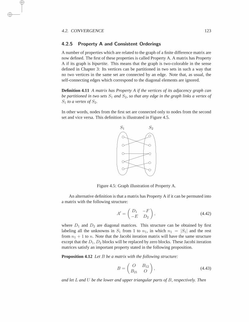
4.2. CONVERGENCE 123
4.2.5 Property A and Consistent Orderings
A number of properties which are related to the graph of a finite difference matrix arenow defined. The first of these properties is called Property A. A matrix has PropertyA if its graph isbipartite. This means that the graph is two-colorable in the sensedefined in Chapter 3: Its vertices can be partitioned in two sets in such a way thatno two vertices in the same set are connected by an edge. Note that, as usual, theself-connecting edges which correspond to the diagonal elements are ignored.
Definition 4.11 A matrix has Property A if the vertices of its adjacency graph canbe partitioned in two setsS1 andS2, so that any edge in the graph links a vertex ofS1 to a vertex ofS2.
In other words, nodes from the first set are connected only to nodes from the secondset and vice versa. This definition is illustrated in Figure 4.5.
S2S1
Figure 4.5: Graph illustration of Property A.
An alternative definition is that a matrix has Property A if it can be permuted intoa matrix with the following structure:
A′ =
(D1 −F−E D2
)
, (4.42)
whereD1 andD2 are diagonal matrices. This structure can be obtained by firstlabeling all the unknowns inS1 from 1 to n1, in which n1 = |S1| and the restfrom n1 + 1 to n. Note that the Jacobi iteration matrix will have the same structureexcept that theD1, D2 blocks will be replaced by zero blocks. These Jacobi iterationmatrices satisfy an important property stated in the following proposition.
Proposition 4.12 LetB be a matrix with the following structure:
B =
(O B12
B21 O
)
, (4.43)
and letL andU be the lower and upper triangular parts ofB, respectively. Then
124 CHAPTER 4. BASIC ITERATIVE METHODS
1. If µ is an eigenvalue ofB, then so is−µ.
2. The eigenvalues of the matrix
B(α) = αL+1
αU
defined forα 6= 0 are independent ofα.
Proof. The first property is shown by simply observing that if(
xv
)is an eigenvector
associated withµ, then(
x−v
)
is an eigenvector ofB associated with the eigenvalue−µ.
Consider the second property. For anyα, the matrixB(α) is similar toB, i.e.,B(α) = XBX−1 with X defined by
X =
(1 OO α
)
.
This proves the desired result
A definition which generalizes this important property isconsistently ordered matri-ces. Varga [293] calls a consistently ordered matrix one for which the eigenvaluesof B(α) are independent ofα. Another definition given by Young [322] considersa specific class of matrices which generalize this property. We will use this defini-tion here. Unlike Property A, the consistent ordering property dependson the initialordering of the unknowns.
Definition 4.13 A matrix is said to be consistently ordered if the vertices of its adja-cency graph can be partitioned inp setsS1, S2, . . ., Sp with the property that anytwo adjacent verticesi and j in the graph belong to two consecutive partitionsSk
andSk′ , with k′ = k − 1, if j < i, andk′ = k + 1, if j > i.
It is easy to show that consistently ordered matrices satisfy property A: thefirst coloris made up of all the partitionsSi with odd i and the second with the partitionsSi
with eveni.
Example 4.2. Block tridiagonal matrices of the form
T =
D1 T12
T21 D2 T23
T32 D3. ..
. . . . .. Tp−1,p
Tp,p−1 Dp
whose diagonal blocksDi are diagonal matrices are calledT -matrices. Clearly, suchmatrices are consistently ordered. Note that matrices of the form (4.42) area partic-ular case withp = 2.

4.2. CONVERGENCE 125
Consider now a general, consistently ordered matrix. By definition, there isper-mutationπ of 1, 2, . . . , n which is the union ofp disjoint subsets
π = π1
⋃
π2 . . .⋃
πp (4.44)
with the property that ifaij 6= 0, j 6= i andi belongs toπk, thenj belongs toπk±1
depending on whetheri < j or i > j. This permutationπ can be used to permuteA symmetrically. IfP is the permutation matrix associated with the permutationπ,then clearly
A′ = P TAP
is aT -matrix.Not every matrix that can be symmetrically permuted into aT -matrix is con-
sistently ordered. The important property here is that the partitionπi preservesthe order of the indicesi, j of nonzero elements. In terms of the adjacency graph,there is a partition of the graph with the property that an oriented edgei, j fromi to j always points to a set with a larger index ifj > i, or a smaller index oth-erwise. In particular, a very important consequence is that edges corresponding tothe lower triangular part will remain so in the permuted matrix. The same is truefor the upper triangular part. Indeed, if a nonzero element in the permutedmatrixis a′i′,j′ = aπ−1(i),π−1(j) 6= 0 with i′ > j′, then by definition of the permutationπ(i′) > π(j′), or i = π(π−1(i)) > j = π(π−1(j)). Because of the order preserva-tion, it is necessary thati > j. A similar observation holds for the upper triangularpart. Therefore, this results in the following proposition.
Proposition 4.14 If a matrixA is consistently ordered, then there exists a permuta-tion matrixP such thatP TAP is aT -matrix and
(P TAP )L = P TALP, (P TAP )U = P TAUP (4.45)
in whichXL represents the (strict) lower part ofX andXU the (strict) upper part ofX.
With the above property it can be shown that for consistently ordered matricesthe eigenvalues ofB(α) as defined in Proposition 4.12 are also invariant with respectto α.
Proposition 4.15 LetB be the Jacobi iteration matrix associated with a consistentlyordered matrixA, and letL andU be the lower and upper triangular parts ofB,respectively. Then the eigenvalues of the matrix
B(α) = αL+1
αU
defined forα 6= 0 do not depend onα.
126 CHAPTER 4. BASIC ITERATIVE METHODS
Proof. First transformB(α) into aT -matrix using the permutationπ in (4.44) pro-vided by the previous proposition
P TB(α)P = αP TLP +1
αP TUP.
From the previous proposition, the lower part ofP TBP is preciselyL′ = P TLP .Similarly, the upper part isU ′ = P TUP , the lower and upper parts of the associatedT -matrix. Therefore, we only need to show that the property is true for aT -matrix.
In this case, for anyα, the matrixB(α) is similar toB. This means thatB(α) =XBX−1 with X being equal to
X =
1αI
α2I.. .
αp−1I
,
where the partitioning is associated with the subsetsπ1, . . . , πp respectively.
Note thatT -matrices and matrices with the structure (4.42) are two particularcases of matrices which fulfill the assumptions of the above proposition. There are anumber of well known properties related to Property A and consistent orderings. Forexample, it is possible to show that,
• Property A is invariant under symmetric permutations.
• A matrix has Property A if and only if there is a permutation matrixP suchthatA′ = P−1AP is consistently ordered.
Consistently ordered matrices satisfy an important property which relates theeigenvalues of the corresponding SOR iteration matrices to those of the Jacobi iter-ation matrices. The main theorem regarding the theory for SOR is a consequence ofthe following result proved by Young [322]. Remember that
MSOR = (D − ωE)−1 (ωF + (1− ω)D)
= (I − ωD−1E)−1(ωD−1F + (1− ω)I
).
Theorem 4.16 Let A be a consistently ordered matrix such thataii 6= 0 for i =1, . . . , n, and letω 6= 0. Then ifλ is a nonzero eigenvalue of the SOR iterationmatrixMSOR, any scalarµ such that
(λ+ ω − 1)2 = λω2µ2 (4.46)
is an eigenvalue of the Jacobi iteration matrixB. Conversely, ifµ is an eigenvalueof the Jacobi matrixB and if a scalarλ satisfies (4.46), thenλ is an eigenvalue ofMSOR.

4.3. ALTERNATING DIRECTION METHODS 127
Proof. DenoteD−1E byL andD−1F byU , so that
MSOR = (I − ωL)−1 (ωU + (1− ω)I)
and the Jacobi iteration matrix is merelyL + U . Writing thatλ is an eigenvalueyields
det(λI − (I − ωL)−1(ωU + (1− ω)I)
)= 0
which is equivalent to
det (λ(I − ωL)− (ωU + (1− ω)I)) = 0
ordet ((λ+ ω − 1)I − ω(λL+ U)) = 0.
Sinceω 6= 0, this can be rewritten as
det
(λ+ ω − 1
ωI − (λL+ U)
)
= 0,
which means that(λ+ω−1)/ω is an eigenvalue ofλL+U . SinceA is consistentlyordered, the eigenvalues ofλL + U which are equal toλ1/2(λ1/2L + λ−1/2U) arethe same as those ofλ1/2(L + U), whereL + U is the Jacobi iteration matrix. Theproof follows immediately.
This theorem allows us to compute an optimal value forω, which can be shownto be equal to
ωopt =2
1 +√
1− ρ(B)2. (4.47)
A typical SOR procedure starts with someω, for example,ω = 1, then proceeds witha number of SOR steps with thisω. The convergence rate for the resulting iterates isestimated providing an estimate forρ(B) using Theorem 4.16. A betterω is then ob-tained from the formula (4.47), and the iteration restarted. Further refinements of theoptimalω are calculated and retrofitted in this manner as the algorithm progresses.
4.3 Alternating Direction Methods
The Alternating Direction Implicit (ADI) method was introduced in the mid-1950sby Peaceman and Rachford [226] specifically for solving equations arising from fi-nite difference discretizations of elliptic and parabolic Partial Differential Equations.Consider a partial differential equation of elliptic type
∂
∂x
(
a(x, y)∂u(x, y)
∂x
)
+∂
∂y
(
b(x, y)∂u(x, y)
∂y
)
= f(x, y) (4.48)
on a rectangular domain with Dirichlet boundary conditions. The equations are dis-cretized with centered finite differences usingn + 2 points in thex direction andm+ 2 points in they direction, This results in the system of equations
Hu + V u = b, (4.49)
128 CHAPTER 4. BASIC ITERATIVE METHODS
in which the matricesH andV represent the three-point central difference approxi-mations to the operators
∂
∂x
(
a(x, y)∂
∂x
)
and∂
∂y
(
b(x, y)∂
∂y
)
,
respectively. In what follows, the same notation is used to represent the discretizedversion of the unknown functionu.
The ADI algorithm consists of iterating by solving (4.49) in thex andy direc-tions alternatively as follows.
ALGORITHM 4.3 Peaceman-Rachford (PR) ADI
1. Fork = 0., 1, . . . , until convergence Do:2. Solve:(H + ρkI)uk+ 1
2= (ρkI − V )uk + b
3. Solve:(V + ρkI)uk+1 = (ρkI −H)uk+ 12
+ b
4. EndDo
Here,ρk, k = 1, 2, . . ., is a sequence of positive acceleration parameters.The specific case whereρk is chosen to be a constantρ deserves particular atten-
tion. In this case, we can formulate the above iteration in the usual form of (4.28)with
G = (V + ρI)−1(H − ρI)(H + ρI)−1(V − ρI), (4.50)
f = (V + ρI)−1[I − (H − ρI)(H + ρI)−1
]b (4.51)
or, whenρ > 0, in the form (4.22) with
M =1
2ρ(H + ρI)(V + ρI), N =
1
2ρ(H − ρI)(V − ρI). (4.52)
Note that (4.51) can be rewritten in a simpler form; see Exercise 5.The ADI algorithm is often formulated for solving the time-dependent Partial
Differential Equation
∂u
∂t=
∂
∂x
(
a(x, y)∂u
∂x
)
+∂
∂y
(
b(x, y)∂u
∂y
)
(4.53)
on the domain(x, y, t) ∈ Ω × [0, T ] ≡ (0, 1) × (0, 1) × [0, T ]. The initial andboundary conditions are:
u(x, y, 0) = x0(x, y), ∀(x, y) ∈ Ω, (4.54)
u(x, y, t) = g(x, y, t), ∀(x, y) ∈ ∂Ω, t > 0, (4.55)
where∂Ω is the boundary of the unit squareΩ. The equations are discretized withrespect to the space variablesx andy as before, resulting in a system of OrdinaryDifferential Equations:
du
dt= Hu+ V u, (4.56)
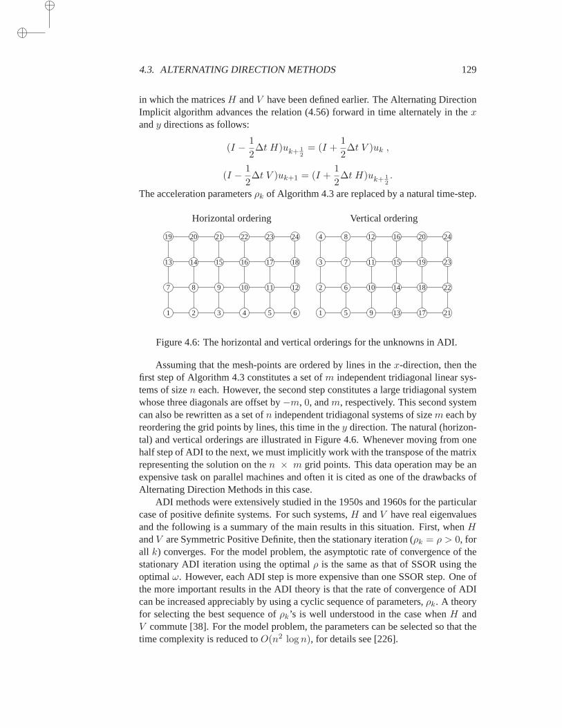
4.3. ALTERNATING DIRECTION METHODS 129
in which the matricesH andV have been defined earlier. The Alternating DirectionImplicit algorithm advances the relation (4.56) forward in time alternately in thexandy directions as follows:
(I − 1
2∆t H)uk+ 1
2= (I +
1
2∆t V )uk ,
(I − 1
2∆t V )uk+1 = (I +
1
2∆t H)uk+ 1
2.
The acceleration parametersρk of Algorithm 4.3 are replaced by a natural time-step.
Horizontal ordering
1 2 3 4 5 6
7 8 9 10 11 12
13 14 15 16 17 18
19 20 21 22 23 24
Vertical ordering
1
2
3
4
5
6
7
8
9
10
11
12
13
14
15
16
17
18
19
20
21
22
23
24
Figure 4.6: The horizontal and vertical orderings for the unknowns in ADI.
Assuming that the mesh-points are ordered by lines in thex-direction, then thefirst step of Algorithm 4.3 constitutes a set ofm independent tridiagonal linear sys-tems of sizen each. However, the second step constitutes a large tridiagonal systemwhose three diagonals are offset by−m, 0, andm, respectively. This second systemcan also be rewritten as a set ofn independent tridiagonal systems of sizem each byreordering the grid points by lines, this time in they direction. The natural (horizon-tal) and vertical orderings are illustrated in Figure 4.6. Whenever moving from onehalf step of ADI to the next, we must implicitly work with the transpose of the matrixrepresenting the solution on then × m grid points. This data operation may be anexpensive task on parallel machines and often it is cited as one of the drawbacks ofAlternating Direction Methods in this case.
ADI methods were extensively studied in the 1950s and 1960s for the particularcase of positive definite systems. For such systems,H andV have real eigenvaluesand the following is a summary of the main results in this situation. First, whenHandV are Symmetric Positive Definite, then the stationary iteration (ρk = ρ > 0, forall k) converges. For the model problem, the asymptotic rate of convergence of thestationary ADI iteration using the optimalρ is the same as that of SSOR using theoptimalω. However, each ADI step is more expensive than one SSOR step. One ofthe more important results in the ADI theory is that the rate of convergence ofADIcan be increased appreciably by using a cyclic sequence of parameters, ρk. A theoryfor selecting the best sequence ofρk’s is well understood in the case whenH andV commute [38]. For the model problem, the parameters can be selected so that thetime complexity is reduced toO(n2 log n), for details see [226].

130 CHAPTER 4. BASIC ITERATIVE METHODS
PROBLEMS
P-4.1 Consider ann× n tridiagonal matrix of the form
Tα =
α −1−1 α −1
−1 α −1−1 α −1
−1 α −1−1 α
, (4.57)
whereα is a real parameter.
a. Verify that the eigenvalues ofTα are given by
λj = α− 2 cos (jθ) j = 1, . . . , n,
whereθ =
π
n+ 1
and that an eigenvector associated with eachλj is
qj = [sin(jθ), sin(2jθ), . . . , sin(njθ)]T.
Under what condition onα does this matrix become positive definite?
b. Now takeα = 2. How does this matrix relate to the matrices seen in Chapter 2forone-dimensional problems?
(i) Will the Jacobi iteration converge for this matrix? If so, what will its conver-gence factor be?
(ii) Will the Gauss-Seidel iteration converge for this matrix? If so, what will itsconvergence factor be?
(iii) For which values ofω will the SOR iteration converge?
P-4.2 Prove that the iteration matrixGω of SSOR, as defined by (4.13), can be expressed as
Gω = I − ω(2− ω)(D − ωF )−1D(D − ωE)−1A.
Deduce the expression (4.27) for the preconditioning matrix associated with the SSOR itera-tion.
P-4.3 LetA be a matrix with a positive diagonalD.
a. Obtain an expression equivalent to that of (4.13) forGω but which involves the matricesSE ≡ D−1/2ED−1/2 andSF ≡ D−1/2FD−1/2.
b. Show that
D1/2GωD−1/2 = (I − ωSF )−1(I − ωSE)−1(ωSE + (1− ω)I)(ωSF + (1− ω)I)
c. Now assume that in addition to having a positive diagonal,A is symmetric. Prove thatthe eigenvalues of the SSOR iteration matrixGω are real and nonnegative.
4.3. ALTERNATING DIRECTION METHODS 131
P-4.4 Let
A =
D1 −F2
−E2 D2 −F3
−E3 D3.. .
. . ... . −Fm
−Em Dm
,
where theDi blocks are nonsingular matrices which are not necessarily diagonal.
a. What are theblock Jacobiandblock Gauss-Seideliteration matrices?
b. Show a result similar to that in Proposition 4.15 for the Jacobi iteration matrix.
c. Show also that forω = 1 (1) the block Gauss-Seidel and block Jacobi iterations eitherboth converge or both diverge, and (2) when they both converge, then the block Gauss-Seidel iteration is (asymptotically) twice as fast as the block Jacobi iteration.
P-4.5 According to formula (4.23), thef vector in iteration (4.22) should be equal toM−1b,whereb is the right-hand side andM is given in (4.52). Yet, formula (4.51) gives a differentexpression forf . Reconcile the two results, i.e., show that the expression (4.51) can also berewritten as
f = 2ρ(V + ρI)−1(H + ρI)−1b.
P-4.6 Show that a matrix has Property A if and only if there is a permutation matrixP suchthatA′ = P−1AP is consistently ordered.
P-4.7 Consider a matrixA which is consistently ordered. Show that the asymptotic conver-gence rate for Gauss-Seidel is double that of the Jacobi iteration.
P-4.8 A matrix of the form
B =
0 E 00 0 FH 0 0
is called a three-cyclic matrix.
a. What are the eigenvalues ofB? (Express them in terms of eigenvalues of a certainmatrix which depends onE, F , andH.)
b. Assume that a matrixA has the formA = D +B, whereD is a nonsingular diagonalmatrix, andB is three-cyclic. How can the eigenvalues of the Jacobi iteration matrixbe related to those of the Gauss-Seidel iteration matrix? How does the asymptoticconvergence rate of the Gauss-Seidel iteration compare with that of the Jacobi iterationmatrix in this case?
c. Answer the same questions as in (b) for the case when SOR replaces the Gauss-Seideliteration.
d. Generalize the above results top-cyclic matrices, i.e., matrices of the form
B =
0 E1
0 E2
0. ..0 Ep−1
Ep 0
.

132 CHAPTER 4. BASIC ITERATIVE METHODS
NOTES AND REFERENCES. Two good references for the material covered in this chapter are Varga[293] and and Young [322]. Although relaxation-type methods were very popular up to the 1960s,they are now mostly used as preconditioners, a topic which will be seen in detail in Chapters 9 and10. One of the main difficulties with these methods is finding an optimal relaxation factor for generalmatrices. Theorem 4.7 is due to Ostrowski. For details on the use of Gershgorin’s theorem in eigenvalueproblems, see [246]. The original idea of the ADI method is described in[226] and those results on theoptimal parameters for ADI can be found in [38]. A comprehensive text on this class of techniques canbe found in [300].

Chapter 5
PROJECTION METHODS
Most of the existing practical iterative techniques for solving large linear systems of equations
utilize a projection process in one way or another. A projection process represents a canonical
way for extracting an approximation to the solution of a linear system from a subspace. This
chapter describes these techniques in a very general framework and presents some theory. The
one-dimensional case is covered in detail at the end of the chapter, as it provides a good preview
of the more complex projection processes to be seen in later chapters.
5.1 Basic Definitions and Algorithms
Consider the linear systemAx = b, (5.1)
whereA is ann× n real matrix. In this chapter, the same symbolA is often used todenote the matrix and the linear mapping inR
n that it represents. The idea ofpro-jection techniquesis to extract an approximate solution to the above problem from asubspace ofRn. If K is this subspace ofcandidate approximants, orsearch subspace,and ifm is its dimension, then, in general,m constraints must be imposed to be ableto extract such an approximation. A typical way of describing these constraints isto imposem (independent) orthogonality conditions. Specifically, the residual vec-tor b − Ax is constrained to be orthogonal tom linearly independent vectors. Thisdefines another subspaceL of dimensionm which will be called thesubspace ofconstraintsor left subspacefor reasons that will be explained below. This simpleframework is common to many different mathematical methods and is known as thePetrov-Galerkin conditions.
There are two broad classes of projection methods:orthogonalandoblique. Inan orthogonal projection technique, the subspaceL is the same asK. In an obliqueprojection method,L is different fromK and may be totally unrelated to it. Thisdistinction is rather important and gives rise to different types of algorithms.
133
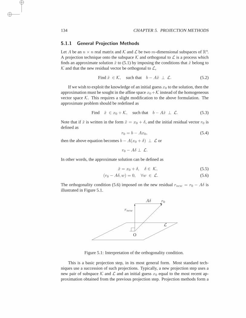
134 CHAPTER 5. PROJECTION METHODS
5.1.1 General Projection Methods
LetA be ann× n real matrix andK andL be twom-dimensional subspaces ofRn.
A projection technique onto the subspaceK and orthogonal toL is a process whichfinds an approximate solutionx to (5.1) by imposing the conditions thatx belong toK and that the new residual vector be orthogonal toL,
Find x ∈ K, such that b−Ax ⊥ L. (5.2)
If we wish to exploit the knowledge of an initial guessx0 to the solution, then theapproximation must be sought in the affine spacex0+K instead of the homogeneousvector spaceK. This requires a slight modification to the above formulation. Theapproximate problem should be redefined as
Find x ∈ x0 +K, such that b−Ax ⊥ L. (5.3)
Note that ifx is written in the formx = x0 + δ, and the initial residual vectorr0 isdefined as
r0 = b−Ax0, (5.4)
then the above equation becomesb−A(x0 + δ) ⊥ L or
r0 −Aδ ⊥ L.
In other words, the approximate solution can be defined as
x = x0 + δ, δ ∈ K, (5.5)
(r0 −Aδ,w) = 0, ∀w ∈ L. (5.6)
The orthogonality condition (5.6) imposed on the new residualrnew = r0 − Aδ isillustrated in Figure 5.1.
L
r0-Aδ
6rnew
O
Figure 5.1: Interpretation of the orthogonality condition.
This is a basic projection step, in its most general form. Most standard tech-niques use a succession of such projections. Typically, a new projectionstep uses anew pair of subspaceK andL and an initial guessx0 equal to the most recent ap-proximation obtained from the previous projection step. Projection methods form a
5.1. BASIC DEFINITIONS AND ALGORITHMS 135
unifying framework for many of the well known methods in scientific computing.Infact, virtually all of the basic iterative techniques seen in the previous chapter can beconsidered projection techniques. Whenever an approximation is definedviam de-grees of freedom (subspaceK) andm constraints (SubspaceL), a projection processresults.
Example 5.1. In the simplest case, an elementary Gauss-Seidel step as defined by(4.6) is nothing but a projection step withK = L = spanei. These projectionsteps are cycled fori = 1, . . . , n until convergence. See Exercise 1 for an alternativeway of selecting the sequence ofei’s.
Orthogonal projection methods correspond to the particular case when thetwosubspacesL andK are identical. The distinction is particularly important in theHermitian case since we are guaranteed that the projected problem will be Hermitianin this situation, as will be seen shortly. In addition, a number of helpful theoreticalresults are true for the orthogonal case. WhenL = K, the Petrov-Galerkin conditionsare often called the Galerkin conditions.
5.1.2 Matrix Representation
Let V = [v1, . . . , vm], ann × m matrix whose column-vectors form a basis ofKand, similarly,W = [w1, . . . , wm], ann ×m matrix whose column-vectors form abasis ofL. If the approximate solution is written as
x = x0 + V y,
then the orthogonality condition leads immediately to the following system of equa-tions for the vectory:
W TAV y = W T r0.
If the assumption is made that them×mmatrixW TAV is nonsingular, the followingexpression for the approximate solutionx results,
x = x0 + V (W TAV )−1W T r0. (5.7)
In many algorithms, the matrixW TAV does not have to be formed since it is avail-able as a by-product of the algorithm. A prototype projection technique is repre-sented by the following algorithm.
ALGORITHM 5.1 Prototype Projection Method
1. Until convergence, Do:2. Select a pair of subspacesK andL3. Choose basesV = [v1, . . . , vm] andW = [w1, . . . , wm] for K andL4. r := b−Ax5. y := (W TAV )−1W T r6. x := x+ V y7. EndDo
136 CHAPTER 5. PROJECTION METHODS
The approximate solution is defined only when the matrixW TAV is nonsingu-lar, a property that is not guaranteed to be true even whenA is nonsingular.
Example 5.2. As an example, consider the matrix
A =
(O II I
)
,
whereI is them×m identity matrix andO is them×m zero matrix, and letV =W = [e1, e2, . . . , em]. AlthoughA is nonsingular, the matrixW TAV is preciselytheO block in the upper-left corner ofA and is therefore singular.
It can be easily verified thatW TAV is nonsingular if and only if no vector ofthe subspaceAK is orthogonal to the subspaceL. We have encountered a similarcondition when defining projector operators in Chapter 1. There are two importantparticular cases where the nonsingularity ofW TAV is guaranteed. These are dis-cussed in the following proposition.
Proposition 5.1 LetA, L, andK satisfy either one of the two following conditions,
i. A is positive definite andL = K, or
ii. A is nonsingular andL = AK.
Then the matrixB = W TAV is nonsingular for any basesV andW of K andL,respectively.
Proof. Consider first the case (i). LetV be any basis ofK andW be any basis ofL.In fact, sinceL andK are the same,W can always be expressed asW = V G, whereG is a nonsingularm×m matrix. Then
B = W TAV = GTV TAV.
SinceA is positive definite, so isV TAV , see Chapter 1, and this shows thatB isnonsingular.
Consider now case (ii). LetV be any basis ofK andW be any basis ofL. SinceL = AK,W can be expressed in this case asW = AV G, whereG is a nonsingularm×m matrix. Then
B = W TAV = GT (AV )TAV. (5.8)
SinceA is nonsingular, then×mmatrixAV is of full rank and as a result,(AV )TAVis nonsingular. This, along with (5.8), shows thatB is nonsingular.
Now consider the particular case whereA is symmetric (real) and an orthogonalprojection technique is used. In this situation, the same basis can be used forL andK, which are identical subspaces, and the projected matrix, which isB = V TAV , issymmetric. In addition, if the matrixA is Symmetric Positive Definite, then so isB.
5.2. GENERAL THEORY 137
5.2 General Theory
This section gives some general theoretical results without being specificabout thesubspacesK andL which are used. The goal is to learn about the quality of theapproximation obtained from a general projection process. Two main tools are usedfor this. The first is to exploit optimality properties of projection methods. Theseproperties are induced from those properties of projectors seen in Section 1.12.4 ofChapter 1. The second tool consists of interpreting the projected problemwith thehelp of projection operators in an attempt to extract residual bounds.
5.2.1 Two Optimality Results
In this section, two important optimality results will be established that are satisfiedby the approximate solutions in some cases. Consider first the case whenA is SPD.
Proposition 5.2 Assume thatA is Symmetric Positive Definite andL = K. Then avectorx is the result of an (orthogonal) projection method ontoK with the startingvectorx0 if and only if it minimizes theA-norm of the error overx0 +K, i.e., if andonly if
E(x) = minx∈x0+K
E(x),
whereE(x) ≡ (A(x∗ − x), x∗ − x)1/2.
Proof. As was seen in Section 1.12.4, forx to be the minimizer ofE(x), it is neces-sary and sufficient thatx∗ − x beA-orthogonal to all the subspaceK. This yields
(A(x∗ − x), v) = 0, ∀v ∈ K,
or, equivalently,(b−Ax, v) = 0, ∀v ∈ K,
which is the Galerkin condition defining an orthogonal projection process for theapproximationx.
We now take up the case whenL is defined byL = AK.
Proposition 5.3 Let A be an arbitrary square matrix and assume thatL = AK.Then a vectorx is the result of an (oblique) projection method ontoK orthogonallytoL with the starting vectorx0 if and only if it minimizes the2-norm of the residualvectorb−Ax overx ∈ x0 +K, i.e., if and only if
R(x) = minx∈x0+K
R(x),
whereR(x) ≡ ‖b−Ax‖2.
138 CHAPTER 5. PROJECTION METHODS
Proof. As was seen in Section 1.12.4, forx to be the minimizer ofR(x), it is nec-essary and sufficient thatb − Ax be orthogonal to all vectors of the formv = Ay,wherey belongs toK, i.e.,
(b−Ax, v) = 0, ∀v ∈ AK,
which is precisely the Petrov-Galerkin condition that defines the approximate solu-tion x.
It is worthwhile to point out thatA need not be nonsingular in the above proposition.WhenA is singular there may be infinitely many vectorsx satisfying the optimalitycondition.
5.2.2 Interpretation in Terms of Projectors
We now return to the two important particular cases singled out in the previoussec-tion, namely, the casesL = K andL = AK. In these cases, the result of theprojection process can be interpreted easily in terms of actions of orthogonal pro-jectors on the initial residual or initial error. Consider the second case first, as it isslightly simpler. Letr0 be the initial residualr0 = b − Ax0, andr = b − Ax theresidual obtained after the projection process withL = AK. Then,
r = b−A(x0 + δ) = r0 −Aδ. (5.9)
In addition,δ is obtained by enforcing the condition thatr0 − Aδ be orthogonal toAK. Therefore, the vectorAδ is the orthogonal projection of the vectorr0 onto thesubspaceAK. This is illustrated in Figure 5.2. Hence, the following proposition canbe stated.
Proposition 5.4 Let x be the approximate solution obtained from a projection pro-cess ontoK orthogonally toL = AK, and letr = b−Ax be the associated residual.Then,
r = (I − P )r0, (5.10)
whereP denotes the orthogonal projector onto the subspaceAK.
A result of the proposition is that the 2-norm of the residual vector obtained afterone projection step will not exceed the initial 2-norm of the residual, i.e.,
‖r‖2 ≤ ‖r0‖2,
a result which has been established already. This class of methods may be termedresidual projectionmethods.
Now consider the case whereL = K andA is Symmetric Positive Definite. Letd0 = x∗ − x0 be the initial error, wherex∗ denotes the exact solution to the systemand, similarly, letd = x∗− x wherex = x0 +δ is the approximate solution resultingfrom the projection step. Then (5.9) yields the relation
Ad = r = A(d0 − δ),
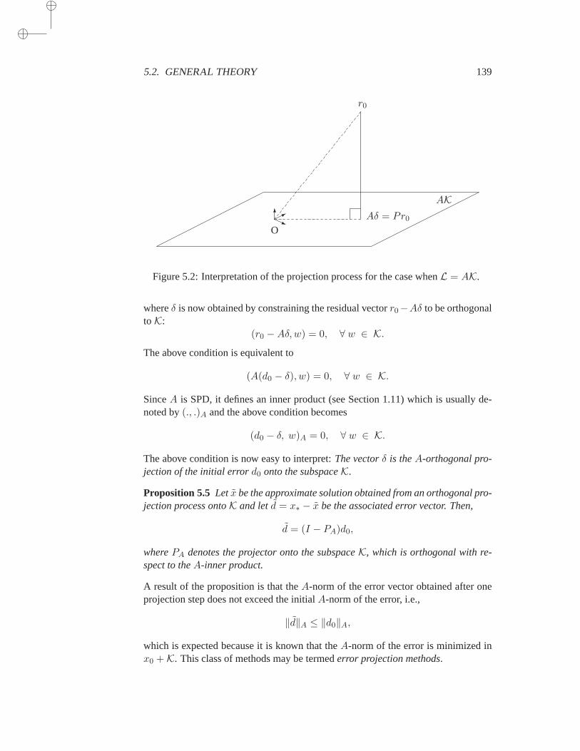
5.2. GENERAL THEORY 139
r0
Aδ = Pr0
AK
O
6*j
Figure 5.2: Interpretation of the projection process for the case whenL = AK.
whereδ is now obtained by constraining the residual vectorr0−Aδ to be orthogonaltoK:
(r0 −Aδ,w) = 0, ∀ w ∈ K.The above condition is equivalent to
(A(d0 − δ), w) = 0, ∀ w ∈ K.
SinceA is SPD, it defines an inner product (see Section 1.11) which is usually de-noted by(., .)A and the above condition becomes
(d0 − δ, w)A = 0, ∀ w ∈ K.
The above condition is now easy to interpret:The vectorδ is theA-orthogonal pro-jection of the initial errord0 onto the subspaceK.
Proposition 5.5 Let x be the approximate solution obtained from an orthogonal pro-jection process ontoK and letd = x∗ − x be the associated error vector. Then,
d = (I − PA)d0,
wherePA denotes the projector onto the subspaceK, which is orthogonal with re-spect to theA-inner product.
A result of the proposition is that theA-norm of the error vector obtained after oneprojection step does not exceed the initialA-norm of the error, i.e.,
‖d‖A ≤ ‖d0‖A,
which is expected because it is known that theA-norm of the error is minimized inx0 +K. This class of methods may be termederror projection methods.
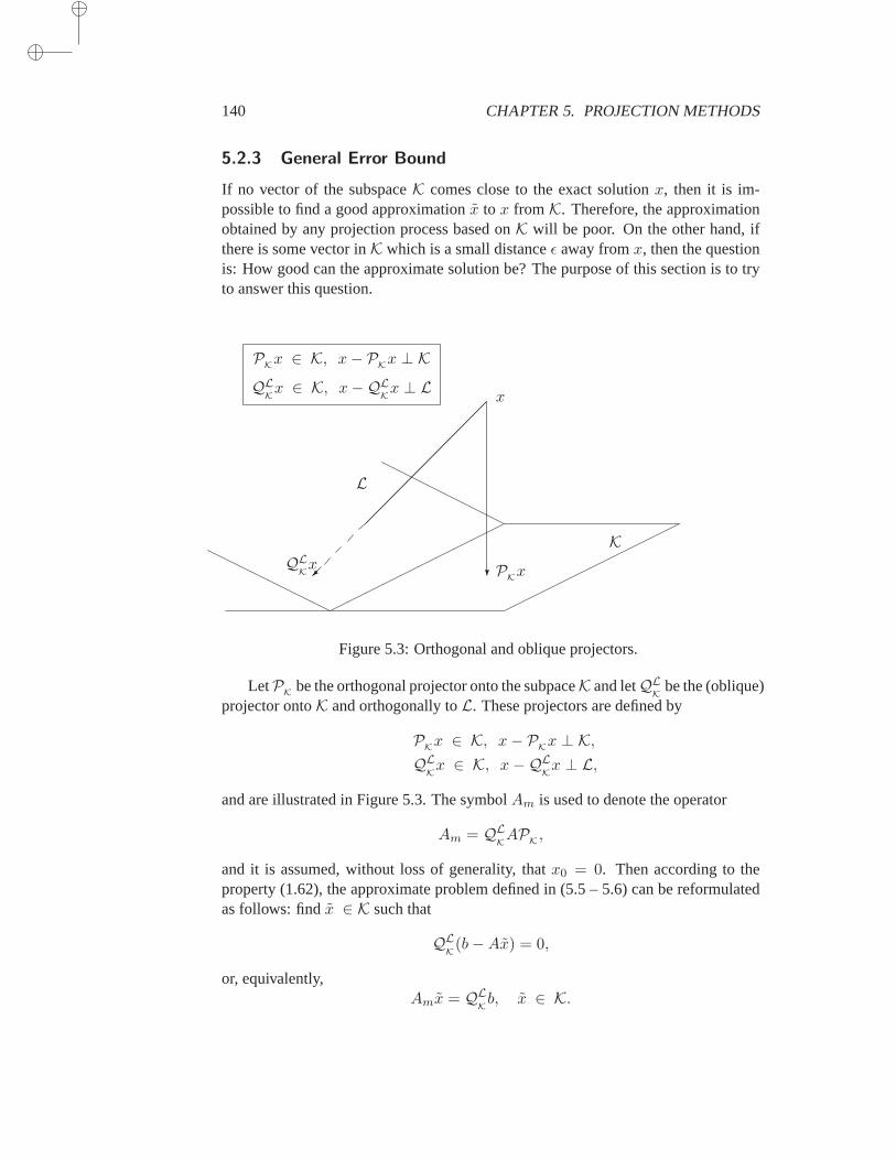
140 CHAPTER 5. PROJECTION METHODS
5.2.3 General Error Bound
If no vector of the subspaceK comes close to the exact solutionx, then it is im-possible to find a good approximationx to x fromK. Therefore, the approximationobtained by any projection process based onK will be poor. On the other hand, ifthere is some vector inK which is a small distanceǫ away fromx, then the questionis: How good can the approximate solution be? The purpose of this section is totryto answer this question.
K
L
?
x
PKxQL
Kx
PKx ∈ K, x− P
Kx ⊥ K
QLKx ∈ K, x−QL
Kx ⊥ L
Figure 5.3: Orthogonal and oblique projectors.
LetPK
be the orthogonal projector onto the subpaceK and letQLK
be the (oblique)projector ontoK and orthogonally toL. These projectors are defined by
PKx ∈ K, x− P
Kx ⊥ K,
QLKx ∈ K, x−QL
Kx ⊥ L,
and are illustrated in Figure 5.3. The symbolAm is used to denote the operator
Am = QLKAP
K,
and it is assumed, without loss of generality, thatx0 = 0. Then according to theproperty (1.62), the approximate problem defined in (5.5 – 5.6) can be reformulatedas follows: findx ∈ K such that
QLK(b−Ax) = 0,
or, equivalently,Amx = QL
Kb, x ∈ K.

5.2. GENERAL THEORY 141
Thus, ann-dimensional linear system is approximated by anm-dimensional one.The following proposition examines what happens in the particular case when the
subspaceK is invariant underA. This is a rare occurrence in practice, but the resulthelps in understanding the breakdown behavior of the methods to be considered inlater chapters.
Proposition 5.6 Assume thatK is invariant underA, x0 = 0, andb belongs toK.Then the approximate solution obtained from any (oblique or orthogonal) projectionmethod ontoK is exact.
Proof. An approximate solutionx is defined by
QLK(b−Ax) = 0,
wherex is a nonzero vector inK. The right-hand sideb is inK, so we haveQLKb = b.
Similarly, x belongs toK which is invariant underA, and therefore,QLKAx = Ax.
Then the above equation becomes
b−Ax = 0,
showing thatx is an exact solution.
The result can be extended trivially to the case wherex0 6= 0. The required assump-tion in this case is that the initial residualr0 = b − Ax0 belongs to the invariantsubspaceK.
An important quantity for the convergence properties of projection methodsisthe distance‖(I − P
K)x∗‖2 of the exact solutionx∗ from the subspaceK. This
quantity plays a key role in the analysis of projection methods. Note that the solutionx∗ cannot be well approximated fromK, if ‖(I − P
K)x∗‖2 is not small because
‖x− x∗‖2 ≥ ‖(I − PK)x∗‖2.
The fundamental quantity‖(I − PK)x∗‖2/‖x∗‖2 is thesineof the acute angle be-
tween the solutionx∗ and the subspaceK. The following theorem establishes anupper bound for the residual norm of theexactsolution with respect to the approxi-mate operatorAm.
Theorem 5.7 Let γ = ‖QLKA(I − P
K)‖2 and assume thatb is a member ofK and
x0 = 0. Then the exact solutionx∗ of the original problem is such that
‖b−Amx∗‖2 ≤ γ‖(I − PK)x∗‖2. (5.11)
Proof. Sinceb ∈ K, then
b−Amx∗ = QLK(b−AP
Kx∗)
= QLK
(Ax∗ −APKx∗)
= QLKA(x∗ − PK
x∗)
= QLKA(I − P
K)x∗.
142 CHAPTER 5. PROJECTION METHODS
Noting thatI − PK
is a projector, it follows that
‖b−Amx∗‖2 = ‖QLKA(I − P
K)(I − P
K)x∗‖2
≤ ‖QLKA(I − P
K)‖2‖(I − PK
)x∗‖2,
which completes the proof.
It is useful to consider a matrix interpretation of the theorem. We consider onlythe particular case of orthogonal projection methods (L = K). Assume thatV isunitary, i.e., that the basisv1, . . . , vm is orthonormal, and thatW = V . Observethatb = V V T b. Equation (5.11) can be represented in the basisV as
‖b− V (V TAV )V Tx∗‖2 ≤ γ‖(I − PK)x∗‖2.
However,
‖b− V (V TAV )V Tx∗‖2 = ‖V (V T b− (V TAV )V Tx∗‖2= ‖V T b− (V TAV )V Tx∗‖2.
Thus, the projection of the exact solution has a residual norm with respect to thematrixB = V TAV , which is of the order of‖(I − P
K)x∗‖2.
5.3 One-Dimensional Projection Processes
This section examines simple examples provided by one-dimensional projectionpro-cesses. In what follows, the vectorr denotes the residual vectorr = b − Ax for thecurrent approximationx. To avoid subscripts, arrow notation is used to denotevectorupdates. Thus, “x ← x + αr” means “computex + αr and overwrite the result onthe currentx.” (This is known as a SAXPY operation.)
One-dimensional projection processes are defined when
K = spanv and L = spanw,
wherev andw are two vectors. In this case, the new approximation takes the formx← x+ αv and the Petrov-Galerkin conditionr −Aδ ⊥ w yields
α =(r, w)
(Av,w). (5.12)
Following are three popular choices to be considered.
5.3.1 Steepest Descent
The steepest descent algorithm is defined for the case where the matrixA is Sym-metric Positive Definite. It consists of taking at each stepv = r andw = r. Thisyields the following iterative procedure:
r ← b−Ax,α← (r, r)/(Ar, r)x← x+ αr.

5.3. ONE-DIMENSIONAL PROJECTION PROCESSES 143
However, the above procedure requires two matrix-by-vector products and this can bereduced to only one by rearranging the computation slightly. The variation consistsof computingr differently as is shown next.
ALGORITHM 5.2 Steepest Descent Algorithm
1. Computer = b−Ax andp = Ar2. Until convergence, Do:3. α← (r, r)/(p, r)4. x← x+ αr5. r ← r − αp6. computep := Ar7. EndDo
Each step of the above iteration minimizes
f(x) = ‖x− x∗‖2A = (A(x− x∗), (x− x∗)),
over all vectors of the formx + αd, whered is the negative of the gradient direc-tion−∇f . The negative of the gradient direction islocally the direction that yieldsthe fastest rate of decrease forf . Next, we prove that convergence is guaranteedwhenA is SPD. The result is a consequence of the following lemma known as theKantorovich inequality.
Lemma 5.8 (Kantorovich inequality) LetB be any Symmetric Positive Definite realmatrix andλmax, λmin its largest and smallest eigenvalues. Then,
(Bx, x)(B−1x, x)
(x, x)2≤ (λmax + λmin)2
4 λmaxλmin, ∀x 6= 0. (5.13)
Proof. Clearly, it is equivalent to show that the result is true for any unit vectorx.SinceB is symmetric, it is unitarily similar to a diagonal matrix,B = QTDQ, and
(Bx, x)(B−1x, x) = (QTDQx, x)(QTD−1Qx, x) = (DQx,Qx)(D−1Qx,Qx).
Settingy = Qx = (y1, . . . , yn)T , andβi = y2i , note that
λ ≡ (Dy, y) =n∑
i=1
βiλi
is a convex combination of the eigenvaluesλi, i = 1, . . . , n. The following relationholds,
(Bx, x)(B−1x, x) = λψ(y) with ψ(y) = (D−1y, y) =n∑
i=1
βi1
λi.
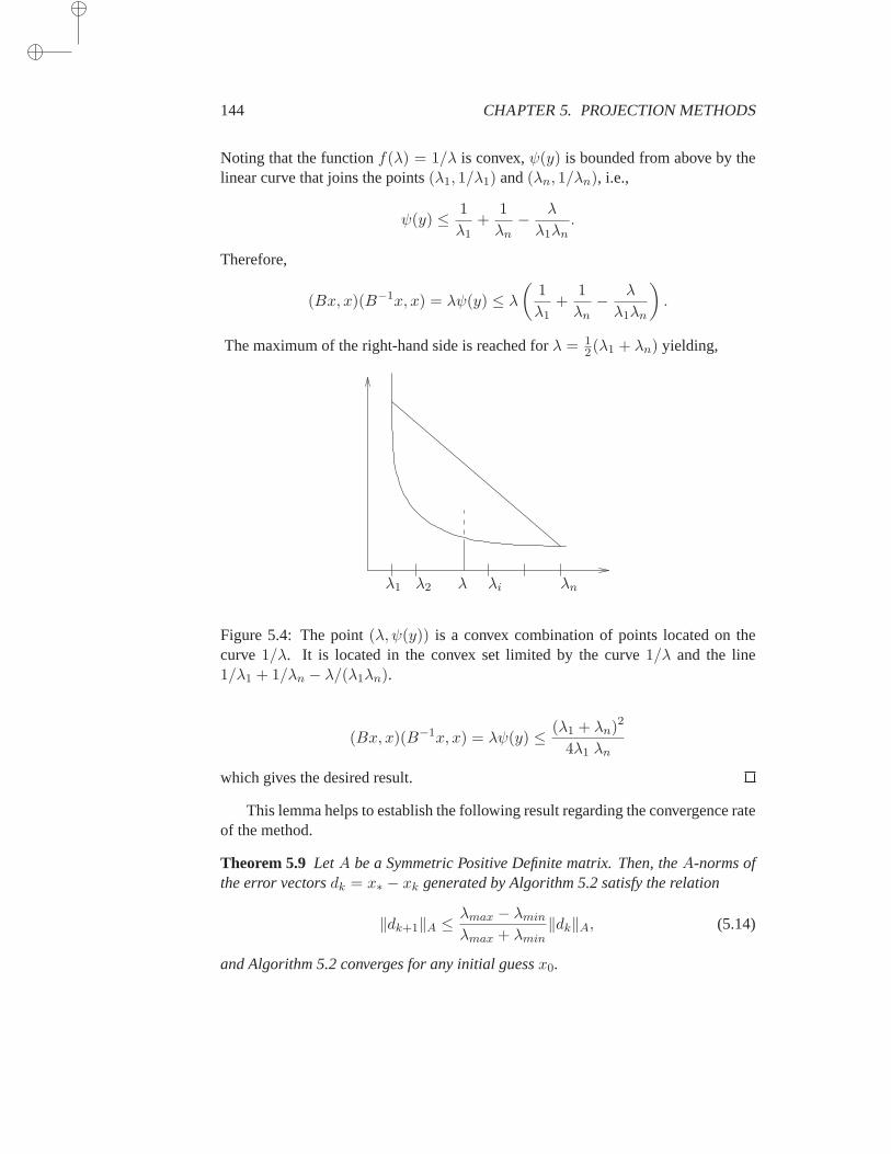
144 CHAPTER 5. PROJECTION METHODS
Noting that the functionf(λ) = 1/λ is convex,ψ(y) is bounded from above by thelinear curve that joins the points(λ1, 1/λ1) and(λn, 1/λn), i.e.,
ψ(y) ≤ 1
λ1+
1
λn− λ
λ1λn.
Therefore,
(Bx, x)(B−1x, x) = λψ(y) ≤ λ(
1
λ1+
1
λn− λ
λ1λn
)
.
The maximum of the right-hand side is reached forλ = 12(λ1 + λn) yielding,
λ1 λ2 λi λnλ
Figure 5.4: The point(λ, ψ(y)) is a convex combination of points located on thecurve 1/λ. It is located in the convex set limited by the curve1/λ and the line1/λ1 + 1/λn − λ/(λ1λn).
(Bx, x)(B−1x, x) = λψ(y) ≤ (λ1 + λn)2
4λ1 λn
which gives the desired result.
This lemma helps to establish the following result regarding the convergence rateof the method.
Theorem 5.9 LetA be a Symmetric Positive Definite matrix. Then, theA-norms ofthe error vectorsdk = x∗ − xk generated by Algorithm 5.2 satisfy the relation
‖dk+1‖A ≤λmax − λmin
λmax + λmin‖dk‖A, (5.14)
and Algorithm 5.2 converges for any initial guessx0.
5.3. ONE-DIMENSIONAL PROJECTION PROCESSES 145
Proof. Start by expanding the square of theA-norm ofdk+1 = dk − αkrk as
‖dk+1‖2A = (dk+1, dk − αkrk)A = (dk+1, dk)A − αk(dk+1, rk)A = (dk+1, rk)
The last equality is due to the orthogonality betweenrk andrk+1. Thus,
‖dk+1‖2A = (dk − αrk, rk)= (A−1rk, rk)− αk(rk, rk)
= ‖dk‖2A(
1− (rk, rk)
(rk, Ark)× (rk, rk)
(rk, A−1rk)
)
.
The result follows by applying the Kantorovich inequality (5.13).
5.3.2 Minimal Residual (MR) Iteration
We now assume thatA is not necessarily symmetric but only positive definite, i.e.,its symmetric partA+AT is Symmetric Positive Definite. Taking at each stepv = randw = Ar, gives the following procedure.
r ← b−Ax,α← (Ar, r)/(Ar,Ar)x← x+ αr.
This procedure can be slightly rearranged again to reduce the number ofmatrix-vector products required to only one per step as was done for the steepest descentalgorithm. This results in in the following algorithm.
ALGORITHM 5.3 Minimal Residual Iteration
1. Computer = b−Ax andp = Ar2. Until convergence, Do:3. α← (p, r)/(p, p)4. x← x+ αr5. r ← r − αp6. computep := Ar7. EndDo
Here, each step minimizesf(x) = ‖b − Ax‖22 in the directionr. The iteration con-verges under the condition thatA is positive definite as is stated in the next theorem.
Theorem 5.10 LetA be a real positive definite matrix, and let
µ = λmin(A+AT )/2, σ = ‖A‖2.
Then the residual vectors generated by Algorithm 5.3 satisfy the relation
‖rk+1‖2 ≤(
1− µ2
σ2
)1/2
‖rk‖2 (5.15)
and Algorithm (5.3) converges for any initial guessx0.
146 CHAPTER 5. PROJECTION METHODS
Proof. We proceed similarly to the steepest descent method, starting with the relation
‖rk+1‖22 = (rk − αkArk, rk − αkArk) (5.16)
= (rk − αkArk, rk)− αk(rk − αkArk, Ark). (5.17)
By construction, the new residual vectorrk−αkArk must be orthogonal to the searchdirectionArk, and, as a result, the second term in the right-hand side of the aboveequation vanishes and we obtain
‖rk+1‖22 = (rk − αkArk, rk)
= (rk, rk)− αk(Ark, rk)
= ‖rk‖22(
1− (Ark, rk)
(rk, rk)
(Ark, rk)
(Ark, Ark)
)
(5.18)
= ‖rk‖22(
1− (Ark, rk)2
(rk, rk)2‖rk‖22‖Ark‖22
)
.
From Theorem 1.34, it can be stated that
(Ax, x)
(x, x)≥ µ > 0, (5.19)
whereµ = λmin(A + AT )/2. The desired result follows immediately by using theinequality‖Ark‖2 ≤ ‖A‖2 ‖rk‖2.
There are alternative ways of obtaining inequalities that prove convergence. Forexample, starting from (5.18), (5.19) can be used again for the term(Ark, rk)/(rk, rk)and similarly, we can write
(Ax, x)
(Ax,Ax)=
(Ax,A−1(Ax))
(Ax,Ax)≥ λmin
(A−1 +A−T
2
)
> 0,
sinceA−1 is also positive definite. This would yield the inequality
‖rk+1‖22 ≤(1− µ(A)µ(A−1)
)‖rk‖22, (5.20)
in whichµ(B) = λmin(B +BT )/2.Another interesting observation is that if we define
cos ∠k =(Ark, rk)
‖Ark‖2 ‖rk‖2,
then (5.18) can be rewritten as
‖rk+1‖22 = ‖rk‖22(
1− (Ark, rk)
(Ark, Ark)
(Ark, rk)
(rk, rk)
)
= ‖rk‖22(1− cos2 ∠k
)
= ‖rk‖22 sin2 ∠k.
5.4. ADDITIVE AND MULTIPLICATIVE PROCESSES 147
At each step the reduction in the residual norm is equal to thesineof the acute anglebetweenr andAr. The convergence factor is therefore bounded by
ρ = maxx ∈ Rn, x 6=0
sin∠(x,Ax),
in which ∠(x,Ax) is the acute angle betweenx andAx. The maximum angle∠(x,Ax) is guaranteed to be less thanπ/2 whenA is positive definite as the aboveresults show.
5.3.3 Residual Norm Steepest Descent
In the residual norm steepest descent algorithm, the assumption thatA is positivedefinite is relaxed. In fact, the only requirement is thatA is a (square) nonsingularmatrix. At each step the algorithm usesv = AT r andw = Av, giving the followingsequence of operations:
r ← b−Ax, v = AT r,
α← ‖v‖22/‖Av‖22,x← x+ αv.
(5.21)
However, an algorithm based on the above sequence of operations would requirethree matrix-by-vector products, which is three times as many as the other algorithmsseen in this section. The number of matrix-by-vector operations can be reduced totwo per step by computing the residual differently. This variant is as follows.
ALGORITHM 5.4 Residual Norm Steepest Descent
1. Computer := b−Ax2. Until convergence, Do:3. v := AT r4. ComputeAv andα := ‖v‖22/‖Av‖225. x := x+ αv6. r := r − αAv7. EndDo
Here, each step minimizesf(x) = ‖b − Ax‖22 in the direction−∇f . As itturns out, this is equivalent to the steepest descent algorithm of Section 5.3.1 appliedto the normal equationsATAx = AT b. SinceATA is positive definite whenA isnonsingular, then, according to Theorem 5.9, the method will converge wheneverAis nonsingular.
5.4 Additive and Multiplicative Processes
We begin by considering again the block relaxation techniques seen in the previouschapter. To define these techniques, aset-decompositionof S = 1, 2, . . . , n is

148 CHAPTER 5. PROJECTION METHODS
considered as the definition ofp subsetsS1, . . . , Sp of S with
Si ⊆ S,⋃
i=1,···,pSi = S.
Denote byni the size ofSi and define the subsetSi as
Si = mi(1),mi(2), . . . ,mi(ni).
Let Vi be then× ni matrix
Vi = [emi(1), emi(2), . . . , emi(ni)],
where eachej is thej-th column of then× n identity matrix.If the block Jacobi and block Gauss-Seidel algorithms, Algorithms 4.1 and 4.2,
are examined carefully, it can be observed that each individual step in the main loop(lines 2 to 5) represents an orthogonal projection process overKi = spanVi. In-deed, the equation (4.17) is exactly (5.7) withW = V = Vi. This individual projec-tion step modifies only the components corresponding to the subspaceKi. However,the general block Jacobi iteration combines these modifications, implicitly addingthem together, to obtain the next iteratexk+1. Borrowing from the terminology ofdomain decomposition techniques, this will be called anadditive projection proce-dure. Generally, an additive projection procedure can be defined for any sequenceof subspacesKi, not just subspaces spanned by the columns of the identity matrix.The only requirement is that the subspacesKi should be distinct, although they areallowed to overlap.
Let a sequence ofp orthogonal systemsVi be given, with the condition thatspanVi 6= spanVj for i 6= j, and define
Ai = V Ti AVi.
The additive projection procedure can be written as
yi = A−1i V T
i (b−Axk), i = 1, . . . , p ,
xk+1 = xk +
p∑
i=1
Viyi, (5.22)
which leads to the following algorithm.
ALGORITHM 5.5 Additive Projection Procedure
1. Fork = 0, 1, . . . , until convergence, Do:2. Fori = 1, 2, . . . , p Do:3. SolveAiyi = V T
i (b−Axk)4. EndDo5. Setxk+1 = xk +
∑pi=1 Viyi
6. EndDo

5.4. ADDITIVE AND MULTIPLICATIVE PROCESSES 149
Definingrk = b−Axk, the residual vector at stepk, then clearly
rk+1 = b−Axk+1
= b−Axk −p∑
i=1
AVi
(V T
i AVi
)−1V T
i rk
=
[
I −p∑
i=1
AVi
(V T
i AVi
)−1V T
i
]
rk.
Observe that each of thep operators
Pi = AVi
(V T
i AVi
)−1V T
i
represents the projector onto the subspace spanned byAVi, and orthogonal toVi.Often, the additive processes are used in conjunction with an accelerationparameterω, thus (5.22) is replaced by
yi = A−1i V T
i (b−Axk), i = 1, . . . , p ,
xk+1 = xk + ω
p∑
i=1
Viyi.
Even more generally, a different parameterωi can be used for each projection, i.e.,
yi = A−1i V T
i (b−Axk), i = 1, . . . , p,
xk+1 = xk +
p∑
i=1
ωiViyi.
The residual norm in this situation is given by
rk+1 =
(
I −p∑
i=1
ωiPi
)
rk, (5.23)
considering the singleω parameter as a particular case. Exercise 15 gives an exampleof the choice ofωi which has the effect of producing a sequence with decreasingresidual norms.
We now return to the generic case, whereωi = 1, ∀i. A least-squares option canbe defined by taking for each of the subproblemsLi = AKi. In this situation,Pi
becomes an orthogonal projector ontoAKi, since
Pi = AVi
((AVi)
TAVi
)−1(AVi)
T .
It is interesting to note that the residual vector obtained after one outer loopis relatedto the previous residual by
rk+1 =
(
I −p∑
i=1
Pi
)
rk,
150 CHAPTER 5. PROJECTION METHODS
where thePi’s are now orthogonal projectors. In particular, in the ideal situationwhen theAVi’s are orthogonal to each other, and the total rank of thePi’s is n, thenthe exact solution would be obtained in one outer step, since in this situation
I −p∑
i=1
Pi = 0.
Thus, the maximum reduction in the residual norm is achieved when theVi’s areA-orthogonal to one another.
Similar to the Jacobi and Gauss-Seidel iterations, what distinguishes the additiveand multiplicative iterations is that the latter updates the component to be correctedat stepi immediately. Then this updated approximate solution is used to compute theresidual vector needed to correct the next component. The Jacobi iteration uses thesame previous approximationxk to update all the components of the solution. Thus,the analogue of the block Gauss-Seidel iteration can be defined as follows.
ALGORITHM 5.6 Multiplicative Projection Procedure
1. Until convergence, Do:2. Fori = 1, 2, . . . , p Do:3. SolveAiy = V T
i (b−Ax)4. Setx := x+ Viy5. EndDo6. EndDo
5.4. ADDITIVE AND MULTIPLICATIVE PROCESSES 151
PROBLEMS
P-5.1 Consider the linear systemAx = b, whereA is a Symmetric Positive Definite matrix.
a. Consider the sequence of one-dimensional projection processes withK = L = spanei,where the sequence of indicesi is selected in any fashion. Letxnew be a new it-erate after one projection step fromx and letr = b − Ax, d = A−1b − x, anddnew = A−1b− xnew. Show that
(Adnew, dnew) = (Ad, d)− (r, ei)2/aii.
Does this equality, as is, establish convergence of the algorithm?
b. Assume now thati is selected at each projection step to be the index of a componentof largest absolute value in the current residual vectorr = b−Ax. Show that
‖dnew‖A ≤(
1− 1
nκ(A)
)1/2
‖d‖A,
in whichκ(A) is the spectral condition number ofA. [Hint: Use the inequality|eTi r| ≥
n−1/2‖r‖2.] Does this prove that the algorithm converges?
P-5.2 Consider the linear systemAx = b, whereA is a Symmetric Positive Definite matrix.Consider a projection step withK = L = spanv wherev is some nonzero vector. Letxnew be the new iterate after one projection step fromx and letd = A−1b− x, anddnew =A−1b− xnew.
a. Show that(Adnew, dnew) = (Ad, d)− (r, v)2/(Av, v).
Does this equality establish convergence of the algorithm?
b. In Gastinel’s method, the vectorv is selected in such a way that(v, r) = ‖r‖1, e.g., bydefining the components ofv to bevi = sign(eT
i r), wherer = b − Ax is the currentresidual vector. Show that
‖dnew‖A ≤(
1− 1
nκ(A)
)1/2
‖d‖A,
in whichκ(A) is the spectral condition number ofA. Does this prove that the algorithmconverges?
c. Compare the cost of one step of this method with that of cyclic Gauss-Seidel (see Ex-ample 5.1) and that of “optimal” Gauss-Seidel where at each stepK = L = spaneiandi is a component of largest magnitude in the current residual vector.
P-5.3 In Section 5.3.3, it was shown that taking a one-dimensionalprojection techniquewith K = span AT r andL = spanAAT r is mathematically equivalent to using theusual steepest descent algorithm applied to the normal equationsATAx = AT b. Show thatan orthogonalprojection method forATAx = AT b using a subspaceK is mathematicallyequivalent to applying a projection method ontoK, orthogonally toL = AK for solving thesystemAx = b.
P-5.4 Consider the matrix
A =
1 −6 06 2 30 3 2
.
152 CHAPTER 5. PROJECTION METHODS
a. Find a rectangle or square in the complex plane which contains all the eigenvalues ofA, without computing the eigenvalues.
b. Is the Minimal Residual iteration guaranteed to convergefor a linear system with thematrixA?
P-5.5 Consider the linear system(D1 −F−E −D2
)(x1
x2
)
=
(b1b2
)
in whichD1 andD2 are both nonsingular matrices of sizem each.
a. Define an orthogonal projection method using the set of vectorse1, . . . , em, i.e.,L =K = spane1, . . . , em. Write down the corresponding projection step (x1 is modifiedinto x1). Similarly, write the projection step for the second half of the vectors, i.e.,whenL = K = spanem+1, . . . , en.
b. Consider an iteration procedure which consists of performing the two successive half-steps described above until convergence. Show that this iteration is equivalent to a(standard) Gauss-Seidel iteration applied to the originalsystem.
c. Now consider a similar idea in whichK is taken to be the same as before for eachhalf-step andL = AK. Write down the iteration procedure based on this approach.Name another technique to which it is mathematically equivalent.
P-5.6 Consider the linear systemAx = b, whereA is a Symmetric Positive Definite matrix.We define a projection method which uses a two-dimensional space at each step. At a givenstep, takeL = K = spanr,Ar, wherer = b−Ax is the current residual.
a. For a basis ofK use the vectorr and the vectorp obtained by orthogonalizingAragainstr with respect to theA-inner product. Give the formula for computingp (noneed to normalize the resulting vector).
b. Write the algorithm for performing the projection method described above.
c. Will the algorithm converge for any initial guessx0? Justify the answer. [Hint: Exploitthe convergence results for one-dimensional projection techniques.]
P-5.7 Consider projection methods which update at each step the current solution with lin-ear combinations from two directions: the current residualr andAr.
a. Consider an orthogonal projection method, i.e., at each stepL = K = spanr,Ar.Assuming thatA is Symmetric Positive Definite, establish convergence of the algo-rithm.
b. Consider a least-squares projection method in which at each stepK = spanr,Ar andL = AK. Assuming thatA is positive definite (not necessarily symmetric), establishconvergence of the algorithm.
[Hint: The convergence results for any of the one-dimensional projection techniques can beexploited.]
P-5.8 Assume that the (one-dimensional) Minimal Residual iteration of Section 5.3.2 isapplied to a symmetric positive matrixA. Will the method converge? What will the result(5.15) become in this case? Both (5.15) and (5.14) suggest a linear convergence with anestimate for the linear convergence rate given by the formulas. How do these estimated ratescompare for matrices with large condition spectral condition numbers?
P-5.9 The “least-squares” Gauss-Seidel relaxation method defines a relaxation step asxnew =x+ δ ei (same as Gauss-Seidel), but choosesδ to minimize the residual norm ofxnew.
5.4. ADDITIVE AND MULTIPLICATIVE PROCESSES 153
a. Write down the resulting algorithm.
b. Show that this iteration is mathematically equivalent toa Gauss-Seidel iteration appliedto the normal equationsATAx = AT b.
P-5.10 Derive three types of one-dimensional projection algorithms in the same manner aswas done in Section 5.3, by replacing every occurrence of theresidual vectorr by a vectorei, a column of the identity matrix.
P-5.11 Derive three types of one-dimensional projection algorithms in the same manner aswas done in Section 5.3, by replacing every occurrence of theresidual vectorr by a vectorAei, a column of the matrixA. What would be an “optimal” choice fori at each projectionstep? Show that the method is globally convergent in this case.
P-5.12 A minimal residual iteration as defined in Section 5.3.2 can also be defined for anarbitrary search directiond, not necessarily related tor in any way. In this case, we stilldefinee = Ad.
a. Write down the corresponding algorithm.
b. Under which condition are all iterates defined?
c. Under which condition ond does the new iterate make no progress, i.e.,‖rk+1‖2 =‖rk‖2?
d. Write a general sufficient condition which must be satisfiedby d at each step in orderto guarantee convergence.
P-5.13 Consider the following real-valued functions of the vectorvariablex, whereA andb are the coefficient matrix and right-hand system of a given linear systemAx = b andx∗ = A−1b.
a(x) = ‖x∗ − x‖22,f(x) = ‖b−Ax‖22,g(x) = ‖AT b−ATAx‖22,h(x) = 2(b, x)− (Ax, x).
a. Calculate the gradients of all four functions above.
b. How is the gradient ofg related to that off?
c. How is the gradient off related to that ofh whenA is symmetric?
d. How does the functionh relate to theA-norm of the errorx∗−x whenA is SymmetricPositive Definite?
P-5.14 The block Gauss-Seidel iteration can be expressed as a method of successive pro-jections. The subspaceK used for each projection is of the form
K = spanei, ei+1, . . . , ei+p.
What isL? Not too commonly used an alternative is to takeL = AK, which amounts tosolving a least-squares problem instead of a linear system.Develop algorithms for this case.What are the advantages and disadvantages of the two approaches (ignoring convergencerates)?
P-5.15 Let the scalarsωi in the additive projection procedure satisfy the constraintp∑
i=1
ωi = 1. (5.24)
154 CHAPTER 5. PROJECTION METHODS
It is not assumed that eachωi is positive but only that|ωi| ≤ 1 for all i. The residual vectoris given by the Formula (5.23) or, equivalently,
rk+1 =
p∑
i=1
ωi(I − Pi)rk.
a. Show that in the least-squares case, we have‖rk+1‖2 ≤ ‖rk‖2 for any choice ofωi’swhich satisfy the constraint (5.24).
b. We wish to choose a set ofωi’s such that the 2-norm of the residual vectorrk+1 isminimal. Determine this set ofωi’s, assuming that the vectors(I − Pi)rk are alllinearly independent.
c. The “optimal”ωi’s provided in the previous question require the solution ofa p × pSymmetric Positive Definite linear system. Letzi ≡ Viyi be the “search directions”provided by each of the individual projection steps. To avoid this difficulty, a simplerstrategy is used which consists of performingp successive minimal residual iterationsalong these search directions, as is described below.
r := rkFor i = 1, . . . , p Do:
ωi := (r,Azi)/(Azi, Azi)x := x+ ωizi
r := r − ωiAzi
EndDo
Show that‖rk+1‖2 ≤ ‖rk‖2. Give a sufficient condition to ensure global convergence.
P-5.16 Consider the iteration:xk+1 = xk +αkdk, wheredk is a vector called thedirectionof search, andαk is a scalar. It is assumed throughout thatdk is a nonzero vector. Considera method which determinesxk+1 so that the residual‖rk+1‖2 is the smallest possible.
a. Determineαk so that‖rk+1‖2 is minimal.
b. Show that the residual vectorrk+1 obtained in this manner is orthogonal toAdk.
c. Show that the residual vectors satisfy the relation:
‖rk+1‖2 ≤ ‖rk‖2 sin∠(rk, Adk).
d. Assume that at each stepk, we have(rk, Adk) 6= 0. Will the method always converge?
e. Now assume thatA is positive definite and select at each stepdk ≡ rk. Prove that themethod will converge for any initial guessx0.
P-5.17 Consider the iteration:xk+1 = xk +αkdk, wheredk is a vector called thedirectionof search, andαk is a scalar. It is assumed throughout thatdk is a vector which is selectedin the formdk = AT fk wherefk is some nonzero vector. Letx∗ = A−1b be the exactsolution. Now consider a method which at each stepk determinesxk+1 so that the errornorm‖x∗ − xk+1‖2 is the smallest possible.
a. Determineαk so that‖x∗ − xk+1‖2 is minimal and show that the error vectorek+1 =x∗ − xk+1 is orthogonal todk. The expression ofαk should not contain unknownquantities (e.g.,x∗ or ek).
b. Show that‖ek+1‖2 ≤ ‖ek‖2 sin∠(ek, dk).
c. Establish the convergence of the algorithm for anyx0, whenfk ≡ rk for all k.

5.4. ADDITIVE AND MULTIPLICATIVE PROCESSES 155
NOTES AND REFERENCES. Initially, the termprojection methodswas used mainly to describe one--dimensional techniques such as those presented in Section 5.3. An excellent account of what has beendone in the late 1950s and early 1960s can be found in Householder’s book [173] as well as Gastinel[140]. For more general, including nonlinear, projection processes,a good reference is Kranoselskiiand co-authors [192].
Projection techniques are present in different forms in many other areas of scientific computingand can be formulated in abstract Hilbert functional spaces. The termsGalerkinandPetrov-Galerkintechniques are used commonly in finite element methods to describe projection methods on finite ele-ment spaces. The principles are identical to those seen in this chapter.

156 CHAPTER 5. PROJECTION METHODS
Chapter 6
KRYLOV SUBSPACE METHODS PART I
The next two chapters explore a few methods which are considered currently to be among the
most important iterative techniques available for solving large linear systems. These techniques
are based on projection processes, both orthogonal and oblique, onto Krylov subspaces, which
are subspaces spanned by vectors of the form p(A)v where p is a polynomial. In short, these
techniques approximate A−1b by p(A)b, where p is a “good” polynomial. This chapter covers
methods derived from, or related to, the Arnoldi orthogonalization. The next chapter covers
methods based on Lanczos biorthogonalization.
6.1 Introduction
Recall from the previous chapter that a generalprojection methodfor solving thelinear system
Ax = b, (6.1)
extracts an approximate solutionxm from an affine subspacex0 +Km of dimensionm by imposing the Petrov-Galerkin condition
b−Axm ⊥ Lm,
whereLm is another subspace of dimensionm. Here,x0 represents an arbitraryinitial guess to the solution. A Krylov subspace method is a method for which thesubspaceKm is the Krylov subspace
Km(A, r0) = spanr0, Ar0, A2r0, . . . , Am−1r0 ,
wherer0 = b − Ax0. When there is no ambiguity,Km(A, r0) will be denoted byKm. The different versions of Krylov subspace methods arise from different choicesof the subspaceLm and from the ways in which the system ispreconditioned, a topicthat will be covered in detail in later chapters.
Viewed from the angle of approximation theory, it is clear that the approxima-tions obtained from a Krylov subspace method are of the form
A−1b ≈ xm = x0 + qm−1(A)r0 ,
157
158 CHAPTER 6. KRYLOV SUBSPACE METHODS PART I
in which qm−1 is a certain polynomial of degreem − 1. In the simplest case wherex0 = 0, then
A−1b ≈ qm−1(A)b .
In other words,A−1b is approximated byqm−1(A)b.Although all the techniques provide the same type ofpolynomialapproxima-
tions, the choice ofLm, i.e., the constraints used to build these approximations, willhave an important effect on the iterative technique. Two broad choices for Lm giverise to the best-known techniques. The first is simplyLm = Km and the minimum-residual variationLm = AKm. A few of the numerous methods in this category willbe described in this chapter. The second class of methods is based on definingLm
to be a Krylov subspace method associated withAT , namely,Lm = Km(AT , r0).Methods of this class will be covered in the next chapter. There are also block exten-sions of each of these methods termedblock Krylov subspace methods, which willbe discussed only briefly. Note that a projection method may have several differ-ent implementations, giving rise to different algorithms which are all mathematicallyequivalent.
6.2 Krylov Subspaces
In this section we consider projection methods onKrylov subspaces, i.e., subspacesof the form
Km(A, v) ≡ span v,Av,A2v, . . . , Am−1v (6.2)
which will be denoted simply byKm if there is no ambiguity. The dimension ofthe subspace of approximants increases by one at each step of the approximationprocess. A few elementary properties of Krylov subspaces can be established. Afirst property is thatKm is the subspace of all vectors inRn which can be writtenasx = p(A)v, wherep is a polynomial of degree not exceedingm − 1. Recall thatthe minimal polynomial of a vectorv is the nonzero monic polynomialp of lowestdegree such thatp(A)v = 0. The degree of the minimal polynomial ofv with respecttoA is often called thegrade ofv with respect toA, or simply the grade ofv if thereis no ambiguity. A consequence of the Cayley-Hamilton theorem is that the grade ofv does not exceedn. The following proposition is easy to prove.
Proposition 6.1 Letµ be the grade ofv. ThenKµ is invariant underA andKm =Kµ for all m ≥ µ.
It was mentioned above that the dimension ofKm is nondecreasing. In fact, thefollowing proposition determines the dimension ofKm in general.
Proposition 6.2 The Krylov subspaceKm is of dimensionm if and only if the gradeµ of v with respect toA is not less thanm, i.e.,
dim(Km) = m ↔ grade(v) ≥ m. (6.3)
Therefore,dim(Km) = min m, grade(v). (6.4)

6.2. KRYLOV SUBSPACES 159
Proof. The vectorsv,Av, . . . , Am−1v form a basis ofKm if and only if for anyset ofm scalarsαi, i = 0, . . . ,m − 1, where at least oneαi is nonzero, the linearcombination
∑m−1i=0 αiA
iv is nonzero. This is equivalent to the condition that theonly polynomial of degree≤ m − 1 for which p(A)v = 0 is the zero polynomial.The equality (6.4) is a consequence of the previous proposition.
Given a certain subspaceX, recall thatA|X denotes the restriction ofA toX. IfQ is a projector ontoX, thesection of the operatorA in X is the operator fromXonto itself defined byQA|X . The following proposition characterizes the product ofpolynomials ofA by v in terms of the section ofA in Km.
Proposition 6.3 LetQm be any projector ontoKm and letAm be the section ofAtoKm, that is,Am = QmA|Km
. Then for any polynomialq of degree not exceedingm− 1,
q(A)v = q(Am)v ,
and for any polynomial of degree≤ m,
Qmq(A)v = q(Am)v .
Proof. First we prove thatq(A)v = q(Am)v for any polynomialq of degree≤ m−1.It is sufficient to show the property for the monic polynomialsqi(t) ≡ ti, i =0, . . . ,m − 1. The proof is by induction. The property is true for the polynomialq0(t) ≡ 1. Assume that it is true forqi(t) ≡ ti:
qi(A)v = qi(Am)v .
Multiplying the above equation byA on both sides yields
qi+1(A)v = Aqi(Am)v .
If i+ 1 ≤ m− 1 the vector on the left-hand side belongs toKm, and therefore if theabove equation is multiplied on both sides byQm, then
qi+1(A)v = QmAqi(Am)v.
Looking at the right-hand side we observe thatqi(Am)v belongs toKm. Hence,
qi+1(A)v = QmA|Kmqi(Am)v = qi+1(Am)v,
which proves that the property is true fori+1, providedi+1 ≤ m− 1. For the casei + 1 = m, it only remains to show thatQmqm(A)v = qm(Am)v, which followsfrom qm−1(A)v = qm−1(Am)v by simply multiplying both sides byQmA.
160 CHAPTER 6. KRYLOV SUBSPACE METHODS PART I
6.3 Arnoldi’s Method
Arnoldi’s method [9] is an orthogonal projection method ontoKm for general non-Hermitian matrices. The procedure was first introduced in 1951 as a means of reduc-ing a dense matrix into Hessenberg form with a unitary transformation. In his paper,Arnoldi hinted that the eigenvalues of the Hessenberg matrix obtained froma numberof steps smaller thann could provide accurate approximations to some eigenvaluesof the original matrix. It was later discovered that this strategy leads to an efficienttechnique for approximating eigenvalues of large sparse matrices and the techniquewas then extended to the solution of large sparse linear systems of equations. Themethod will first be described theoretically, i.e., assuming exact arithmetic, thenim-plementation details will be addressed.
6.3.1 The Basic Algorithm
Arnoldi’s procedure is an algorithm for building an orthogonal basis of the KrylovsubspaceKm. In exact arithmetic, one variant of the algorithm is as follows:
ALGORITHM 6.1 Arnoldi
1. Choose a vectorv1, such that‖v1‖2 = 12. Forj = 1, 2, . . . ,m Do:3. Computehij = (Avj , vi) for i = 1, 2, . . . , j
4. Computewj := Avj −∑j
i=1 hijvi
5. hj+1,j = ‖wj‖26. If hj+1,j = 0 then Stop7. vj+1 = wj/hj+1,j
8. EndDo
At each step, the algorithm multiplies the previous Arnoldi vectorvj by A andthen orthonormalizes the resulting vectorwj against all previousvi’s by a standardGram-Schmidt procedure. It will stop if the vectorwj computed in line 4 vanishes.This case will be examined shortly. Now a few simple properties of the algorithmare proved.
Proposition 6.4 Assume that Algorithm 6.1 does not stop before them-th step. Thenthe vectorsv1, v2, . . . , vm form an orthonormal basis of the Krylov subspace
Km = spanv1, Av1, . . . , Am−1v1.
Proof. The vectorsvj , j = 1, 2, . . . ,m, are orthonormal by construction. That theyspanKm follows from the fact that each vectorvj is of the formqj−1(A)v1 whereqj−1 is a polynomial of degreej−1. This can be shown by induction onj as follows.The result is clearly true forj = 1, sincev1 = q0(A)v1 with q0(t) ≡ 1. Assume thatthe result is true for all integers≤ j and considervj+1. We have
hj+1,jvj+1 = Avj −j∑
i=1
hijvi = Aqj−1(A)v1 −j∑
i=1
hijqi−1(A)v1 (6.5)
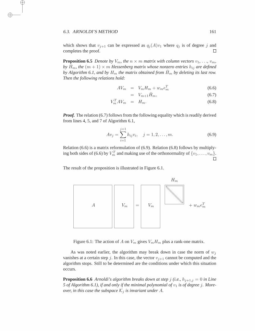
6.3. ARNOLDI’S METHOD 161
which shows thatvj+1 can be expressed asqj(A)v1 whereqj is of degreej andcompletes the proof.
Proposition 6.5 Denote byVm, then ×m matrix with column vectorsv1, . . ., vm,by Hm, the(m + 1) ×m Hessenberg matrix whose nonzero entrieshij are definedby Algorithm 6.1, and byHm the matrix obtained fromHm by deleting its last row.Then the following relations hold:
AVm = VmHm + wmeTm (6.6)
= Vm+1Hm, (6.7)
V TmAVm = Hm. (6.8)
Proof. The relation (6.7) follows from the following equality which is readily derivedfrom lines 4, 5, and 7 of Algorithm 6.1,
Avj =
j+1∑
i=1
hijvi, j = 1, 2, . . . ,m. (6.9)
Relation (6.6) is a matrix reformulation of (6.9). Relation (6.8) follows by multiply-ing both sides of (6.6) byV T
m and making use of the orthonormality ofv1, . . . , vm.
The result of the proposition is illustrated in Figure 6.1.
Vm + wmeTm=A
Hm
Vm
Figure 6.1: The action ofA onVm givesVmHm plus a rank-one matrix.
As was noted earlier, the algorithm may break down in case the norm ofwj
vanishes at a certain stepj. In this case, the vectorvj+1 cannot be computed and thealgorithm stops. Still to be determined are the conditions under which this situationoccurs.
Proposition 6.6 Arnoldi’s algorithm breaks down at stepj (i.e.,hj+1,j = 0 in Line5 of Algorithm 6.1), if and only if the minimal polynomial ofv1 is of degreej. More-over, in this case the subspaceKj is invariant underA.

162 CHAPTER 6. KRYLOV SUBSPACE METHODS PART I
Proof. If the degree of the minimal polynomial isj, thenwj must be equal to zero.Indeed, otherwisevj+1 can be defined and as a resultKj+1 would be of dimensionj+1. Then Proposition 6.2 would imply thatµ ≥ j+1, which is a contradiction. Toprove the converse, assume thatwj = 0. Then the degreeµ of the minimal polyno-mial of v1 is such thatµ ≤ j. Moreover, it is impossible thatµ < j. Otherwise, bythe first part of this proof, the vectorwµ would be zero and the algorithm would havestopped at the earlier step numberµ. The rest of the result follows from Proposition6.1.
A corollary of the proposition is that a projection method onto the subspaceKj
will be exact when a breakdown occurs at stepj. This result follows from Proposition5.6 seen in Chapter 5. It is for this reason that such breakdowns are often calledluckybreakdowns.
6.3.2 Practical Implementations
In the previous description of the Arnoldi process, exact arithmetic was assumed,mainly for simplicity. In practice, much can be gained by using the Modified Gram-Schmidt or the Householder algorithm instead of the standard Gram-Schmidt algo-rithm. With the Modified Gram-Schmidt alternative the algorithm takes the followingform:
ALGORITHM 6.2 Arnoldi-Modified Gram-Schmidt
1. Choose a vectorv1 of norm 12. Forj = 1, 2, . . . ,m Do:3. Computewj := Avj
4. Fori = 1, . . . , j Do:5. hij = (wj , vi)6. wj := wj − hijvi
7. EndDo8. hj+1,j = ‖wj‖2. If hj+1,j = 0 Stop9. vj+1 = wj/hj+1,j
10. EndDo
In exact arithmetic, this algorithm and Algorithm 6.1 are mathematically equivalent.In the presence of round-off the above formulation is much more reliable. However,there are cases where cancellations are so severe in the orthogonalization steps thateven the Modified Gram-Schmidt option is inadequate. In this case, two furtherimprovements can be utilized.
The first improvement resorts to double orthogonalization. Whenever the finalvectorwj obtained at the end of the main loop in the above algorithm has beencomputed, a test is performed to compare its norm with the norm of the initialwj
(which is‖Avj‖2). If the reduction falls below a certain threshold, indicating severecancellation might have occurred, a second orthogonalization is made. It isknown
6.3. ARNOLDI’S METHOD 163
from a result by Kahan that additional orthogonalizations are superfluous (see, forexample, Parlett [224]).
The second improvement is to use a different technique altogether. From thenumerical point of view, one of the most reliable orthogonalization techniques is theHouseholder algorithm. Recall from Chapter 1 that the Householder orthogonaliza-tion uses reflection matrices of the formPk = I − 2wkw
Tk to transform a matrixX
into upper triangular form. In the Arnoldi algorithm, the column vectors of the ma-trix X to be orthonormalized are not available ahead of time. Instead, the next vectoris obtained asAvj , wherevj is the current basis vector. In the Householder algo-rithm an orthogonal columnvi is obtained asP1P2 . . . Piei whereP1, . . . , Pi are theprevious Householder matrices. This vector is then multiplied byA and the previousHouseholder transforms are applied to it. Then, the next Householder transform isdetermined from the resulting vector. This procedure is described in the followingalgorithm, which was originally proposed by Walker [303].
ALGORITHM 6.3 Householder Arnoldi
1. Select a nonzero vectorv; Setz1 = v2. Forj = 1, . . . ,m,m+ 1 Do:3. Compute the Householder unit vectorwj such that4. (wj)i = 0, i = 1, . . . , j − 1 and5. (Pjzj)i = 0, i = j + 1, . . . , n, wherePj = I − 2wjw
Tj
6. hj−1 = Pjzj7. vj = P1P2 . . . Pjej8. If j ≤ m computezj+1 := PjPj−1 . . . P1Avj
9. EndDo
For details regarding the determination of the Householder vectorwj in the thirdto fifth lines and on its use in the sixth to eight lines, see Chapter 1. Recall thatthe matricesPj need not be formed explicitly. To obtainhj−1 from zj in line 6,zero out all the components from positionj + 1 throughn of then-vectorzj andchange itsj-th component, leaving all others unchanged. Thus, then × m matrix[h0, h1, . . . , hm] will have the same structure as the matrixXm of equation (1.27)in Chapter 1. By comparison with the Householder algorithm seen in Chapter 1,we can infer that the above process computes theQR factorization of the matrixv,Av1, Av2, Av3, . . . , Avm. Define
Qj = PjPj−1 . . . P1. (6.10)
The definition ofzj+1 in line 8 of the algorithm yields the relation,
QjAvj = zj+1.
After the next Householder transformationPj+1 is applied in line 6,hj satisfies therelation,
hj = Pj+1zj+1 = Pj+1QjAvj = Qj+1Avj . (6.11)
164 CHAPTER 6. KRYLOV SUBSPACE METHODS PART I
Now observe that since the componentsj + 2, . . . , n of hj are zero, thenPihj = hj
for anyi ≥ j + 2. Hence,
hj = PmPm−1 . . . Pj+2hj = QmAvj , j = 1, . . . ,m.
This leads to the factorization,
Qm[v,Av1, Av2, . . . , Avm] = [h0, h1, . . . , hm] (6.12)
where the matrix[h0, . . . , hm] is n × (m + 1) and is upper triangular andQm isunitary.
It is important to relate the vectorsvi andhi defined in this algorithm with vectorsof the standard Arnoldi process. LetHm be the(m+ 1)× m matrix obtained fromthe firstm + 1 rows of then × m matrix [h1, . . . , hm]. SinceQj+1 is unitary wehaveQ−1
j+1 = QTj+1 and hence, from the relation (6.11)
Avj = QTj+1
j+1∑
i=1
hijei =
j+1∑
i=1
hijQTj+1ei
where eachei is thei-th column of then × n identity matrix. SincePkei = ei fori < k, it is not difficult to see that
QTj+1ei = P1 . . . Pj+1ei = vi, for i ≤ j + 1. (6.13)
This yields the relationAvj =∑j+1
i=1 hijvi, for j = 1, . . . ,m, which can be writtenin matrix form as
AVm = Vm+1Hm.
This is identical with the relation (6.7) obtained with the Gram-Schmidt or ModifiedGram-Schmidt implementation. Thevi’s form an orthonormal basis of the KrylovsubspaceKm and are identical with thevi’s defined by the Arnoldi process, apartfrom a possible sign difference.
Although the Householder algorithm is numerically more viable than the Gram-Schmidt or Modified Gram-Schmidt versions, it is also more expensive. Thecost ofeach of the outer loops, corresponding to thej control variable, is dominated by lines7 and 8. These apply the reflection matricesPi for i = 1, . . . , j to a vector, performthe matrix-vector productAvj , and then apply the matricesPi for i = j, j− 1, . . . , 1to a vector. The application of eachPi to a vector is performed as
(I − 2wiwTi )v = v − σwi with σ = 2wT
i v.
This is essentially the result of a dot-product of lengthn− i+1 followed by a vectorupdate of the same length, requiring a total of about4(n − i + 1) operations foreach application ofPi. Neglecting the last step, the number of operations due to theHouseholder transformations alone approximately totals
m∑
j=1
j∑
i=1
8(n− i+ 1) = 8
m∑
j=1
(
jn− j(j − 1)
2
)
≈ 4m2n− 4
3m3.
6.4. ARNOLDI’S METHOD FOR LINEAR SYSTEMS (FOM) 165
The table below shows the costs of different orthogonalization procedures. GS standsfor Gram-Schmidt, MGS for Modified Gram-Schmidt, MGSR for Modified Gram-Schmidt with reorthogonalization, and HO for Householder.
GS MGS MGSR HO
Flops 2m2n 2m2n 4m2n 4m2n− 43m
3
Storage (m+ 1)n (m+ 1)n (m+ 1)n (m+ 1)n− 12m
2
The number of operations shown for MGSR corresponds to the worst case scenariowhen a second orthogonalization is performed each time. In practice, the numberof operations is usually closer to that of the standard MGS. Regarding storage, thevectorsvi, i = 1, . . . ,m need not be saved. In the algorithms for solving linearsystems, these vectors are needed at the end of the process. This issuewill be coveredwith the Householder implementations of these algorithms. For now, assume thatonly thewi’s are saved. The small gain in memory usage in the Householder versioncan be explained by the diminishing lengths of the vectors required at each step ofthe Householder transformation. However, this difference is negligible relative to thewhole storage requirement of the algorithm, becausem≪ n, typically.
The Householder orthogonalization may be a reasonable choice when developinggeneral purpose, reliable software packages where robustness is acritical criterion.This is especially true for solving eigenvalue problems since the cost of orthogo-nalization is then amortized over several eigenvalue/eigenvector calculations. Whensolving linear systems, the Modified Gram-Schmidt orthogonalization, with a re-orthogonalization strategy based on a measure of the level of cancellation,is morethan adequate in most cases.
6.4 Arnoldi’s Method for Linear Systems (FOM)
Given an initial guessx0 to the original linear systemAx = b, we now consider anorthogonalprojection methodas defined in the previous chapter, which takesL =K = Km(A, r0), with
Km(A, r0) = spanr0, Ar0, A2r0, . . . , Am−1r0, (6.14)
in which r0 = b − Ax0. This method seeks an approximate solutionxm from theaffine subspacex0 +Km of dimensionm by imposing the Galerkin condition
b−Axm ⊥ Km. (6.15)
If v1 = r0/‖r0‖2 in Arnoldi’s method, and we setβ = ‖r0‖2, then
V TmAVm = Hm
by (6.8) andV T
m r0 = V Tm (βv1) = βe1.

166 CHAPTER 6. KRYLOV SUBSPACE METHODS PART I
As a result, the approximate solution using the abovem-dimensional subspaces isgiven by
xm = x0 + Vmym, (6.16)
ym = H−1m (βe1). (6.17)
A method based on this approach and called the Full Orthogonalization Method(FOM) is described next. Modified Gram-Schmidt is used in the Arnoldi procedure.
ALGORITHM 6.4 Full Orthogonalization Method (FOM)
1. Computer0 = b−Ax0, β := ‖r0‖2, andv1 := r0/β2. Define them×m matrixHm = hiji,j=1,...,m; SetHm = 03. Forj = 1, 2, . . . ,m Do:4. Computewj := Avj
5. Fori = 1, . . . , j Do:6. hij = (wj , vi)7. wj := wj − hijvi
8. EndDo9. Computehj+1,j = ‖wj‖2. If hj+1,j = 0 setm := j and Goto 12
10. Computevj+1 = wj/hj+1,j .11. EndDo12. Computeym = H−1
m (βe1) andxm = x0 + Vmym
The above algorithm depends on a parameterm which is the dimension of theKrylov subspace. In practice it is desirable to selectm in a dynamic fashion. Thiswould be possible if the residual norm of the solutionxm is available inexpensively(without having to computexm itself). Then the algorithm can be stopped at theappropriate step using this information. The following proposition gives a result inthis direction.
Proposition 6.7 The residual vector of the approximate solutionxm computed bythe FOM Algorithm is such that
b−Axm = −hm+1,meTmymvm+1
and, therefore,‖b−Axm‖2 = hm+1,m|eTmym|. (6.18)
Proof. We have the relations,
b−Axm = b−A(x0 + Vmym)
= r0 −AVmym
= βv1 − VmHmym − hm+1,meTmymvm+1.
By the definition ofym,Hmym = βe1, and soβv1 − VmHmym = 0 from which theresult follows.
6.4. ARNOLDI’S METHOD FOR LINEAR SYSTEMS (FOM) 167
A rough estimate of the cost of each step of the algorithm is determined as fol-lows. IfNz(A) is the number of nonzero elements ofA, thenm steps of the Arnoldiprocedure will requirem matrix-vector products at the cost of2m × Nz(A). Eachof the Gram-Schmidt steps costs approximately4× j × n operations, which bringsthe total over them steps to approximately2m2n. Thus, on the average, a step ofFOM costs approximately
2Nz(A) + 2mn.
Regarding storage,m vectors of lengthn are required to save the basisVm. Addi-tional vectors must be used to keep the current solution and right-hand side, and ascratch vector for the matrix-vector product. In addition, the Hessenberg matrixHm
must be saved. The total is therefore roughly
(m+ 3)n+m2
2.
In most situationsm is small relative ton, so this cost is dominated by the first term.
6.4.1 Variation 1: Restarted FOM
Consider now the algorithm from a practical viewpoint. Asm increases, the com-putational cost increases at least asO(m2n) because of the Gram-Schmidt orthogo-nalization. The memory cost increases asO(mn). For largen this limits the largestvalue ofm that can be used. There are two remedies. The first is to restart thealgorithm periodically and the second is to “truncate” the orthogonalization in theArnoldi algorithm. In this section we consider the first of these two options, whichis described below.
ALGORITHM 6.5 Restarted FOM (FOM(m))
1. Computer0 = b−Ax0, β = ‖r0‖2, andv1 = r0/β.2. Generate the Arnoldi basis and the matrixHm using the Arnoldi algorithm3. starting withv1.4. Computeym = H−1
m βe1 andxm = x0 + Vmym. If satisfied then Stop.5. Setx0 := xm and go to 1.
There are many possible variations to this basic scheme. One that is generallymore economical in practice is based on the observation that sometimes a smallm issufficient for convergence and sometimes the largest possiblem is necessary. Hence,the idea of averaging over different values ofm. Start the algorithm withm = 1 andincrementm by one in line 5 until a certainmmax is reached, after whichm is resetto one, or kept the same. These variations will not be considered here.
Example 6.1. Table 6.1 shows the results of applying FOM(10) with no precon-ditioning to three of the test problems described in Section 3.7. The column labeledIters shows the total actual number of matrix-vector multiplications (matvecs) re-quired to converge. The stopping criterion used is that the 2-norm of the residual be
168 CHAPTER 6. KRYLOV SUBSPACE METHODS PART I
Matrix Iters Kflops Residual Error
F2DA 109 4442 0.36E-03 0.67E-04
F3D 66 11664 0.87E-03 0.35E-03
ORS 300 13558 0.26E+00 0.71E-04
Table 6.1: A test run of FOM with no preconditioning.
reduced by a factor of107 relative to the 2-norm of the initial residual. A maximumof 300 matvecs are allowed.Kflops is the total number of floating point operationsperformed, in thousands.ResidualandError represent the two-norm of the residualand error vectors, respectively. Note that the method did not succeed insolving thethird problem.
6.4.2 Variation 2: IOM and DIOM
A second alternative to FOM is to truncate the Arnoldi recurrence. Specifically, anintegerk is selected and the following “incomplete” orthogonalization is performed.
ALGORITHM 6.6 Incomplete Orthogonalization Process
1. Forj = 1, 2, . . . ,m Do:2. Computewj := Avj
3. Fori = max1, j − k + 1, . . . , j Do:4. hi,j = (wj , vi)5. wj := wj − hijvi
6. EndDo7. Computehj+1,j = ‖wj‖2 andvj+1 = wj/hj+1,j
8. EndDo
The number of directionsk against which to orthogonalize may be dictated bymemory limitations. The Incomplete Orthogonalization Method (IOM) consists ofperforming the above incomplete orthogonalization procedure and computingan ap-proximate solution using the same formulas (6.16) and (6.17).
ALGORITHM 6.7 IOM Algorithm
Run a modification of Algorithm 6.4 in which the Arnoldi process in lines3 to 11 is replaced by the Incomplete Orthogonalization process and everyother computation remains unchanged.
It is now necessary to keep only thek previousvi vectors. The others are notneeded in the above process and may be discarded. However, the difficulty re-mains that when the solution is computed by formula (6.16), all the vectorsvi for
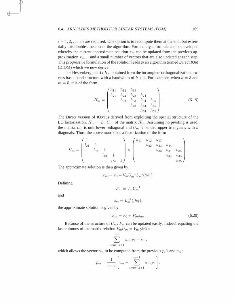
6.4. ARNOLDI’S METHOD FOR LINEAR SYSTEMS (FOM) 169
i = 1, 2, . . . ,m are required. One option is to recompute them at the end, but essen-tially this doubles the cost of the algorithm. Fortunately, a formula can be developedwhereby the current approximate solutionxm can be updated from the previous ap-proximationxm−1 and a small number of vectors that are also updated at each step.Thisprogressiveformulation of the solution leads to an algorithm termedDirect IOM(DIOM) which we now derive.
The Hessenberg matrixHm obtained from the incomplete orthogonalization pro-cess has a band structure with a bandwidth ofk + 1. For example, whenk = 3 andm = 5, it is of the form
Hm =
h11 h12 h13
h21 h22 h23 h24
h32 h33 h34 h35
h43 h44 h45
h54 h55
. (6.19)
The Direct version of IOM is derived from exploiting the special structure of theLU factorization,Hm = LmUm, of the matrixHm. Assuming no pivoting is used,the matrixLm is unit lower bidiagonal andUm is banded upper triangular, withkdiagonals. Thus, the above matrix has a factorization of the form
Hm =
1l21 1
l32 1l43 1
l54 1
×
u11 u12 u13
u22 u23 u24
u33 u34 u35
u44 u45
u55
.
The approximate solution is then given by
xm = x0 + VmU−1m L−1
m (βe1).
DefiningPm ≡ VmU
−1m
andzm = L−1
m (βe1),
the approximate solution is given by
xm = x0 + Pmzm. (6.20)
Because of the structure ofUm, Pm can be updated easily. Indeed, equating thelast columns of the matrix relationPmUm = Vm yields
m∑
i=m−k+1
uimpi = vm,
which allows the vectorpm to be computed from the previouspi’s andvm:
pm =1
umm
[
vm −m−1∑
i=m−k+1
uimpi
]
.
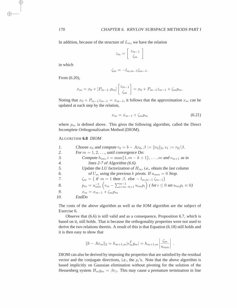
170 CHAPTER 6. KRYLOV SUBSPACE METHODS PART I
In addition, because of the structure ofLm, we have the relation
zm =
[zm−1
ζm
]
in whichζm = −lm,m−1ζm−1.
From (6.20),
xm = x0 + [Pm−1, pm]
[zm−1
ζm
]
= x0 + Pm−1zm−1 + ζmpm.
Noting thatx0 + Pm−1zm−1 = xm−1, it follows that the approximationxm can beupdated at each step by the relation,
xm = xm−1 + ζmpm (6.21)
wherepm is defined above. This gives the following algorithm, called the DirectIncomplete Orthogonalization Method (DIOM).
ALGORITHM 6.8 DIOM
1. Choosex0 and computer0 = b−Ax0, β := ‖r0‖2, v1 := r0/β.2. Form = 1, 2, . . ., until convergence Do:3. Computehim, i = max1,m− k + 1, . . . ,m andvm+1 as in4. lines 2-7 of Algorithm (6.6).5. Update the LU factorization ofHm, i.e., obtain the last column6. ofUm using the previousk pivots. Ifumm = 0 Stop.7. ζm = if m = 1 then β, else− lm,m−1 ζm−18. pm = u−1
mm
(
vm −∑m−1
i=m−k+1 uimpi
)
( for i ≤ 0 setuimpi ≡ 0)
9. xm = xm−1 + ζmpm
10. EndDo
The costs of the above algorithm as well as the IOM algorithm are the subjectofExercise 6.
Observe that (6.6) is still valid and as a consequence, Proposition 6.7, which isbased on it, still holds. That is because the orthogonality properties were not used toderive the two relations therein. A result of this is that Equation (6.18) still holds andit is then easy to show that
‖b−Axm‖2 = hm+1,m|eTmym| = hm+1,m
∣∣∣∣
ζmumm
∣∣∣∣.
DIOM can also be derived by imposing the properties that are satisfied by the residualvector and the conjugate directions, i.e., thepi’s. Note that the above algorithm isbased implicitly on Gaussian elimination without pivoting for the solution of theHessenberg systemHmym = βe1. This may cause a premature termination in line
6.5. GMRES 171
6. Fortunately, an implementation is available which relies on Gaussian eliminationwith partial pivoting. The details of this variant can be found in [240].
Since the residual vector is a scalar multiple ofvm+1 and since thevi’s are nolonger orthogonal, IOM and DIOM are not orthogonal projection techniques. Theycan, however, be viewed as oblique projection techniques ontoKm and orthogonalto an artificially constructed subspace.
Proposition 6.8 IOM and DIOM are mathematically equivalent to a projection pro-cess ontoKm and orthogonally to
Lm = spanz1, z2, . . . , zm
wherezi = vi − (vi, vm+1)vm+1, i = 1, . . . ,m.
Proof. The proof is an immediate consequence of the fact thatrm is a multiple ofvm+1 and by construction,vm+1 is orthogonal to allzi’s defined in the proposition.
The following simple properties can be shown:
• The residual vectorsri, i = 1, . . . ,m, are “locally” orthogonal,
(rj , ri) = 0, for |i− j| ≤ k, i 6= j. (6.22)
• Thepj ’s are locallyA-orthogonal to the Arnoldi vectors, i.e.,
(Apj , vi) = 0 for j − k + 1 < i < j. (6.23)
• For the casek =∞ (full orthogonalization) thepj ’s are semi-conjugate, i.e.,
(Apj , pi) = 0 for i < j. (6.24)
6.5 GMRES
The Generalized Minimum Residual Method (GMRES) is a projection method basedon takingK = Km andL = AKm, in whichKm is them-th Krylov subspace withv1 = r0/‖r0‖2. As seen in Chapter 5, such a technique minimizes the residual normover all vectors inx0 + Km. The implementation of an algorithm based on thisapproach is similar to that of the FOM algorithm. We first describe the basic ideaand then discuss practical details and a few variations.
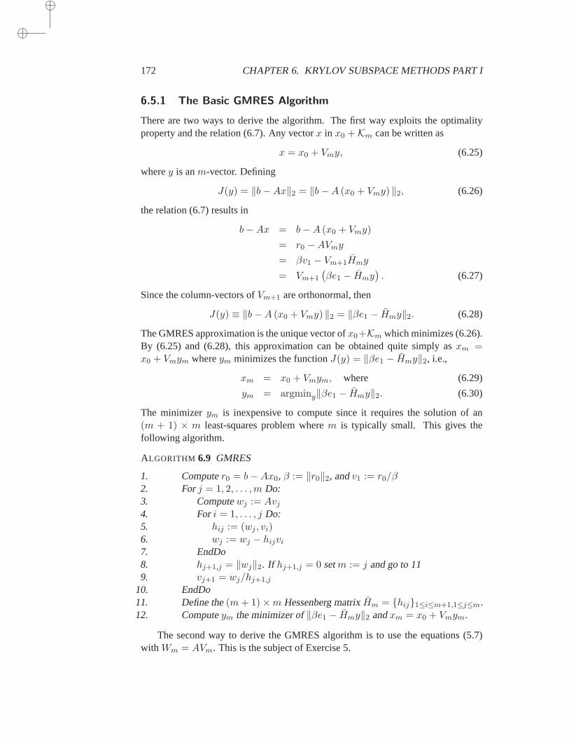
172 CHAPTER 6. KRYLOV SUBSPACE METHODS PART I
6.5.1 The Basic GMRES Algorithm
There are two ways to derive the algorithm. The first way exploits the optimalityproperty and the relation (6.7). Any vectorx in x0 +Km can be written as
x = x0 + Vmy, (6.25)
wherey is anm-vector. Defining
J(y) = ‖b−Ax‖2 = ‖b−A (x0 + Vmy) ‖2, (6.26)
the relation (6.7) results in
b−Ax = b−A (x0 + Vmy)
= r0 −AVmy
= βv1 − Vm+1Hmy
= Vm+1
(βe1 − Hmy
). (6.27)
Since the column-vectors ofVm+1 are orthonormal, then
J(y) ≡ ‖b−A (x0 + Vmy) ‖2 = ‖βe1 − Hmy‖2. (6.28)
The GMRES approximation is the unique vector ofx0+Km which minimizes (6.26).By (6.25) and (6.28), this approximation can be obtained quite simply asxm =x0 + Vmym whereym minimizes the functionJ(y) = ‖βe1 − Hmy‖2, i.e.,
xm = x0 + Vmym, where (6.29)
ym = argminy‖βe1 − Hmy‖2. (6.30)
The minimizerym is inexpensive to compute since it requires the solution of an(m + 1) × m least-squares problem wherem is typically small. This gives thefollowing algorithm.
ALGORITHM 6.9 GMRES
1. Computer0 = b−Ax0, β := ‖r0‖2, andv1 := r0/β2. Forj = 1, 2, . . . ,m Do:3. Computewj := Avj
4. Fori = 1, . . . , j Do:5. hij := (wj , vi)6. wj := wj − hijvi
7. EndDo8. hj+1,j = ‖wj‖2. If hj+1,j = 0 setm := j and go to 119. vj+1 = wj/hj+1,j
10. EndDo11. Define the(m+ 1)×m Hessenberg matrixHm = hij1≤i≤m+1,1≤j≤m.12. Computeym the minimizer of‖βe1 − Hmy‖2 andxm = x0 + Vmym.
The second way to derive the GMRES algorithm is to use the equations (5.7)with Wm = AVm. This is the subject of Exercise 5.
6.5. GMRES 173
6.5.2 The Householder Version
The previous algorithm utilizes the Modified Gram-Schmidt orthogonalization in theArnoldi process. Section 6.3.2 described a Householder variant of theArnoldi pro-cess which is numerically more robust than Gram-Schmidt. Here, we focus on amodification of GMRES which retrofits the Householder orthogonalization. Section6.3.2 explained how to get thevj and the columns ofHm+1 at each step, from theHouseholder-Arnoldi algorithm. SinceVm andHm are the only items needed to ex-tract the approximate solution at the end of the GMRES process, the modificationseems rather straightforward. However, this is only true if thevi’s are stored. In thiscase, line 12 would remain the same and the modification to the algorithm wouldbe in lines 3-11 which are to be replaced by the Householder variant of the Arnoldiprocess. It was mentioned in Section 6.3.2 that it is preferable not to store the vi’sbecause this would double the storage requirement. In this case, a formula must befound to generate the approximate solution in line 12, using only thewi’s, i.e., thePi’s. Let
ym = (η1, η2, · · · , ηm)T ,
so that the solution is of the formxm = x0 + η1v1 + · · ·+ ηmvm. Recall that in theHouseholder variant of the Arnoldi process, eachvj is defined by
vj = P1P2 . . . Pjej .
Using a Horner-like scheme, we obtain
xm = x0 + η1P1e1 + η2P1P2e2 + . . .+ ηmP1P2 . . . Pmem
= x0 + P1 (η1e1 + P2 (η2e2 + . . .+ Pm−1 (ηm−1em−1 + Pmηmem))) .
Therefore, when Householder orthogonalization is used, then line 12 ofthe GMRESalgorithm should be replaced by a step of the form
z := 0 (6.31)
z := Pj (ηjej + z) , j = m,m− 1, . . . , 1 (6.32)
xm = x0 + z. (6.33)
The above step requires roughly as many operations as computing the last Arnoldivectorvm. Therefore, its cost is negligible relative to the cost of the Arnoldi loop.
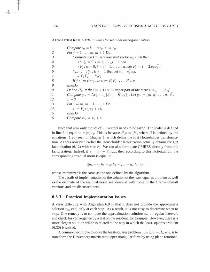
174 CHAPTER 6. KRYLOV SUBSPACE METHODS PART I
ALGORITHM 6.10 GMRES with Householder orthogonalization
1. Computer0 = b−Ax0, z := r0.2. Forj = 1, . . . ,m,m+ 1 Do:3. Compute the Householder unit vectorwj such that4. (wj)i = 0, i = 1, . . . , j − 1 and5. (Pjz)i = 0, i = j + 1, . . . , n wherePj = I − 2wjw
Tj ;
6. hj−1 := Pjz; If j = 1 then letβ := eT1 h0.7. v := P1P2 . . . Pjej .8. If j ≤ m computez := PjPj−1 . . . P1Av,9. EndDo
10. DefineHm = the(m+ 1)×m upper part of the matrix[h1, . . . , hm].11. Computeym = Argminy‖βe1 − Hmy‖2. Let ym = (η1, η2, . . . , ηm)T .12. z := 013. Forj = m,m− 1, . . . , 1 Do:14. z := Pj (ηjej + z),15. EndDo16. Computexm = x0 + z
Note that now only the set ofwj vectors needs to be saved. The scalarβ definedin line 6 is equal to±‖r0‖2. This is becauseP1z = βe1 whereβ is defined by theequations (1.26) seen in Chapter 1, which define the first Householder transforma-tion. As was observed earlier the Householder factorization actually obtains the QRfactorization (6.12) withv = r0. We can also formulate GMRES directly from thisfactorization. Indeed, ifx = x0 + Vmym, then according to this factorization, thecorresponding residual norm is equal to
‖h0 − η1h1 − η2h2 − . . .− ηmhm‖2
whose minimizer is the same as the one defined by the algorithm.The details of implementation of the solution of the least-squares problem as well
as the estimate of the residual norm are identical with those of the Gram-Schmidtversions and are discussed next.
6.5.3 Practical Implementation Issues
A clear difficulty with Algorithm 6.9 is that it does not provide the approximatesolutionxm explicitly at each step. As a result, it is not easy to determine when tostop. One remedy is to compute the approximation solutionxm at regular intervalsand check for convergence by a test on the residual, for example. However, there is amore elegant solution which is related to the way in which the least-squares problem(6.30) is solved.
A common technique to solve the least-squares problemmin ‖βe1−Hmy‖2, is totransform the Hessenberg matrix into upper triangular form by using planerotations.
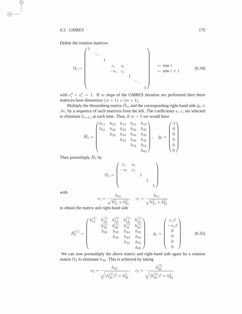
6.5. GMRES 175
Define the rotation matrices
Ωi =
1. . .
1ci si
−si ci1
.. .1
← row i← row i+ 1
(6.34)
with c2i + s2i = 1. If m steps of the GMRES iteration are performed then thesematrices have dimension(m+ 1)× (m+ 1).
Multiply the Hessenberg matrixHm and the corresponding right-hand sideg0 ≡βe1 by a sequence of such matrices from the left. The coefficientssi, ci are selectedto eliminatehi+1,i at each time. Thus, ifm = 5 we would have
H5 =
h11 h12 h13 h14 h15
h21 h22 h23 h24 h25
h32 h33 h34 h35
h43 h44 h45
h54 h55
h65
, g0 =
β00000
.
Then premultiplyH5 by
Ω1 =
c1 s1−s1 c1
11
1
withs1 =
h21√
h211 + h2
21
, c1 =h11
√
h211 + h2
21
to obtain the matrix and right-hand side
H(1)5 =
h(1)11 h
(1)12 h
(1)13 h
(1)14 h
(1)15
h(1)22 h
(1)23 h
(1)24 h
(1)25
h32 h33 h34 h35
h43 h44 h45
h54 h55
h65
, g1 =
c1β−s1β
0000
. (6.35)
We can now premultiply the above matrix and right-hand side again by a rotationmatrixΩ2 to eliminateh32. This is achieved by taking
s2 =h32
√
(h(1)22 )2 + h2
32
, c2 =h
(1)22
√
(h(1)22 )2 + h2
32
.

176 CHAPTER 6. KRYLOV SUBSPACE METHODS PART I
This elimination process is continued until them-th rotation is applied, which trans-forms the problem into one involving the matrix and right-hand side,
H(5)5 =
h(5)11 h
(5)12 h
(5)13 h
(5)14 h
(5)15
h(5)22 h
(5)23 h
(5)24 h
(5)25
h(5)33 h
(5)34 h
(5)35
h(5)44 h
(5)45
h(5)55
0
, g5 =
γ1
γ2
γ3
.
.γ6
. (6.36)
Generally, the scalarsci andsi of theith rotationΩi are defined as
si =hi+1,i
√
(h(i−1)ii )2 + h2
i+1,i
, ci =h
(i−1)ii
√
(h(i−1)ii )2 + h2
i+1,i
. (6.37)
DefineQm the product of matricesΩi,
Qm = ΩmΩm−1 . . .Ω1 (6.38)
and
Rm = H(m)m = QmHm, (6.39)
gm = Qm(βe1) = (γ1, . . . , γm+1)T . (6.40)
SinceQm is unitary,
min ‖βe1 − Hmy‖2 = min ‖gm − Rmy‖2.
The solution to the above least-squares problem is obtained by simply solving thetriangular system resulting from deleting the last row of the matrixRm and right-hand sidegm in (6.36). In addition, it is clear that for the solutiony∗, the “residual”‖βe1− Hmy∗‖ is nothing but the last element of the right-hand side, i.e., the termγ6
in the above illustration.
Proposition 6.9 Letm ≤ n andΩi, i = 1, . . . ,m be the rotation matrices used totransformHm into an upper triangular form. Denote byRm, gm = (γ1, . . . , γm+1)
T
the resulting matrix and right-hand side, as defined by (6.39), (6.40). and byRm, gm
them×m upper triangular matrix andm-dimensional vector obtained fromRm, gm
by deleting their last row and component respectively. Then,
1. The rank ofAVm is equal to the rank ofRm. In particular, if rmm = 0 thenAmust be singular.
2. The vectorym which minimizes‖βe1 − Hmy‖2 is given by
ym = R−1m gm.
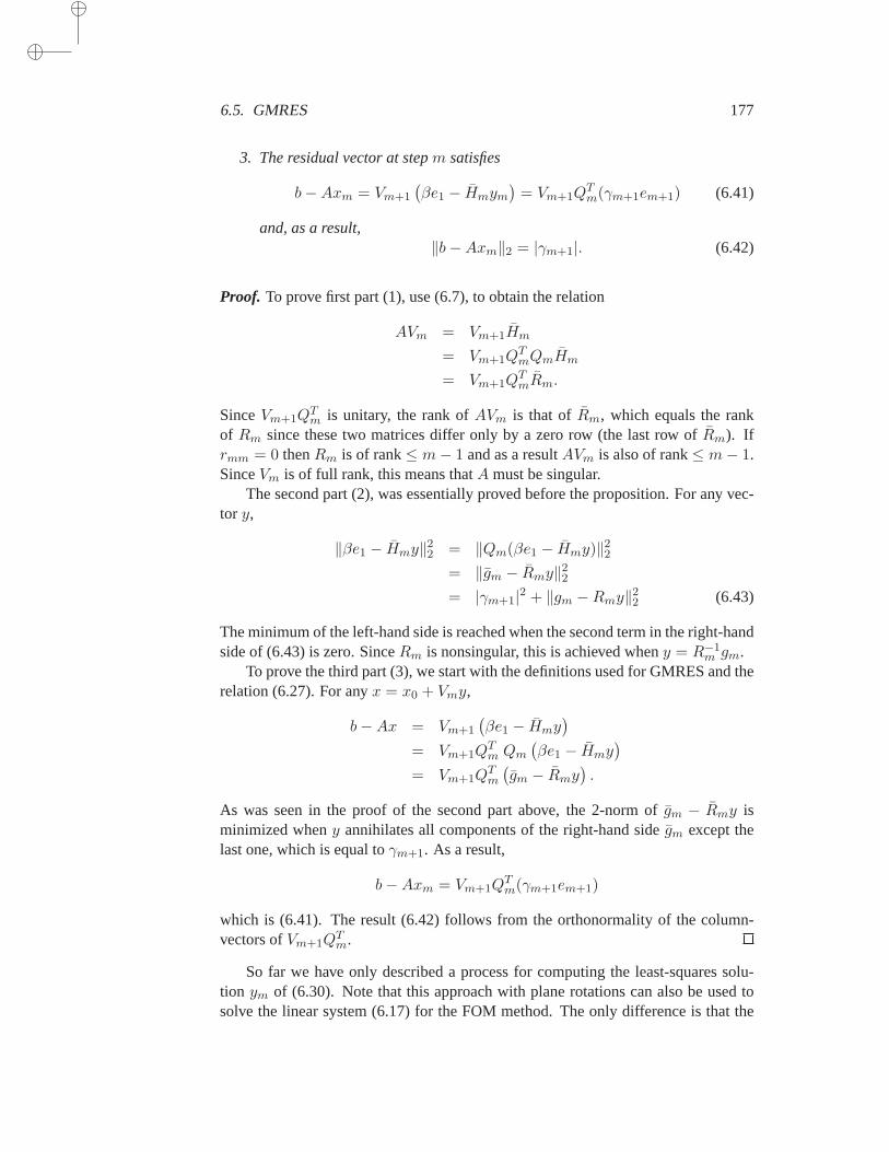
6.5. GMRES 177
3. The residual vector at stepm satisfies
b−Axm = Vm+1
(βe1 − Hmym
)= Vm+1Q
Tm(γm+1em+1) (6.41)
and, as a result,‖b−Axm‖2 = |γm+1|. (6.42)
Proof. To prove first part (1), use (6.7), to obtain the relation
AVm = Vm+1Hm
= Vm+1QTmQmHm
= Vm+1QTmRm.
SinceVm+1QTm is unitary, the rank ofAVm is that of Rm, which equals the rank
of Rm since these two matrices differ only by a zero row (the last row ofRm). Ifrmm = 0 thenRm is of rank≤ m− 1 and as a resultAVm is also of rank≤ m− 1.SinceVm is of full rank, this means thatA must be singular.
The second part (2), was essentially proved before the proposition. For any vec-tor y,
‖βe1 − Hmy‖22 = ‖Qm(βe1 − Hmy)‖22= ‖gm − Rmy‖22= |γm+1|2 + ‖gm −Rmy‖22 (6.43)
The minimum of the left-hand side is reached when the second term in the right-handside of (6.43) is zero. SinceRm is nonsingular, this is achieved wheny = R−1
m gm.To prove the third part (3), we start with the definitions used for GMRES and the
relation (6.27). For anyx = x0 + Vmy,
b−Ax = Vm+1
(βe1 − Hmy
)
= Vm+1QTm Qm
(βe1 − Hmy
)
= Vm+1QTm
(gm − Rmy
).
As was seen in the proof of the second part above, the 2-norm ofgm − Rmy isminimized wheny annihilates all components of the right-hand sidegm except thelast one, which is equal toγm+1. As a result,
b−Axm = Vm+1QTm(γm+1em+1)
which is (6.41). The result (6.42) follows from the orthonormality of the column-vectors ofVm+1Q
Tm.
So far we have only described a process for computing the least-squares solu-tion ym of (6.30). Note that this approach with plane rotations can also be used tosolve the linear system (6.17) for the FOM method. The only difference is that the
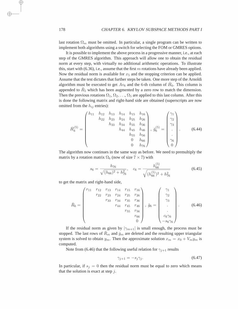
178 CHAPTER 6. KRYLOV SUBSPACE METHODS PART I
last rotationΩm must be omitted. In particular, a single program can be written toimplement both algorithms using a switch for selecting the FOM or GMRES options.
It is possible to implement the above process in a progressive manner, i.e., at eachstep of the GMRES algorithm. This approach will allow one to obtain the residualnorm at every step, with virtually no additional arithmetic operations. To illustratethis, start with (6.36), i.e., assume that the firstm rotations have already been applied.Now the residual norm is available forx5 and the stopping criterion can be applied.Assume that the test dictates that further steps be taken. One more step of theArnoldialgorithm must be executed to getAv6 and the6-th column ofH6. This column isappended toR5 which has been augmented by a zero row to match the dimension.Then the previous rotationsΩ1, Ω2, . . ., Ω5 are applied to this last column. After thisis done the following matrix and right-hand side are obtained (superscripts are nowomitted from thehij entries):
H(5)6 =
h11 h12 h13 h14 h15 h16
h22 h23 h24 h25 h26
h33 h34 h35 h36
h44 h45 h46
h55 h56
0 h66
0 h76
, g(5)6 =
γ1
γ2
γ3
.
.γ6
0
. (6.44)
The algorithm now continues in the same way as before. We need to premultiply thematrix by a rotation matrixΩ6 (now of size7× 7) with
s6 =h76
√
(h66)2 + h276
, c6 =h
(5)66
√
(h(5)66 )2 + h2
76
(6.45)
to get the matrix and right-hand side,
R6 =
r11 r12 r13 r14 r15 r16r22 r23 r24 r25 r26
r33 r34 r35 r36r44 r45 r46
r55 r56r660
, g6 =
γ1
γ2
γ3
.
.c6γ6
−s6γ6
. (6.46)
If the residual norm as given by|γm+1| is small enough, the process must bestopped. The last rows ofRm andgm are deleted and the resulting upper triangularsystem is solved to obtainym. Then the approximate solutionxm = x0 + Vmym iscomputed.
Note from (6.46) that the following useful relation forγj+1 results
γj+1 = −sjγj . (6.47)
In particular, ifsj = 0 then the residual norm must be equal to zero which meansthat the solution is exact at stepj.
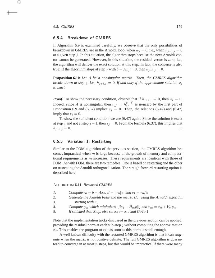
6.5. GMRES 179
6.5.4 Breakdown of GMRES
If Algorithm 6.9 is examined carefully, we observe that the only possibilities ofbreakdown in GMRES are in the Arnoldi loop, whenwj = 0, i.e., whenhj+1,j = 0at a given stepj. In this situation, the algorithm stops because the next Arnoldi vec-tor cannot be generated. However, in this situation, the residual vector iszero, i.e.,the algorithm will deliver the exact solution at this step. In fact, the converse is alsotrue: If the algorithm stops at stepj with b−Axj = 0, thenhj+1,j = 0.
Proposition 6.10 Let A be a nonsingular matrix. Then, the GMRES algorithmbreaks down at stepj, i.e., hj+1,j = 0, if and only if the approximate solutionxj
is exact.
Proof. To show the necessary condition, observe that ifhj+1,j = 0, thensj = 0.Indeed, sinceA is nonsingular, thenrjj = h
(j−1)jj is nonzero by the first part of
Proposition 6.9 and (6.37) impliessj = 0. Then, the relations (6.42) and (6.47)imply thatrj = 0.
To show the sufficient condition, we use (6.47) again. Since the solution is exactat stepj and not at stepj−1, thensj = 0. From the formula (6.37), this implies thathj+1,j = 0.
6.5.5 Variation 1: Restarting
Similar to the FOM algorithm of the previous section, the GMRES algorithm be-comes impractical whenm is large because of the growth of memory and computa-tional requirements asm increases. These requirements are identical with those ofFOM. As with FOM, there are two remedies. One is based on restarting and theotheron truncating the Arnoldi orthogonalization. The straightforward restarting option isdescribed here.
ALGORITHM 6.11 Restarted GMRES
1. Computer0 = b−Ax0, β = ‖r0‖2, andv1 = r0/β2. Generate the Arnoldi basis and the matrixHm using the Arnoldi algorithm3. starting withv14. Computeym which minimizes‖βe1 − Hmy‖2 andxm = x0 + Vmym
5. If satisfied then Stop, else setx0 := xm and GoTo 1
Note that the implementation tricks discussed in the previous section can be applied,providing the residual norm at each sub-stepj without computing the approximationxj . This enables the program to exit as soon as this norm is small enough.
A well known difficulty with the restarted GMRES algorithm is that it canstag-natewhen the matrix is not positive definite. The full GMRES algorithm is guaran-teed to converge in at mostn steps, but this would be impractical if there were many
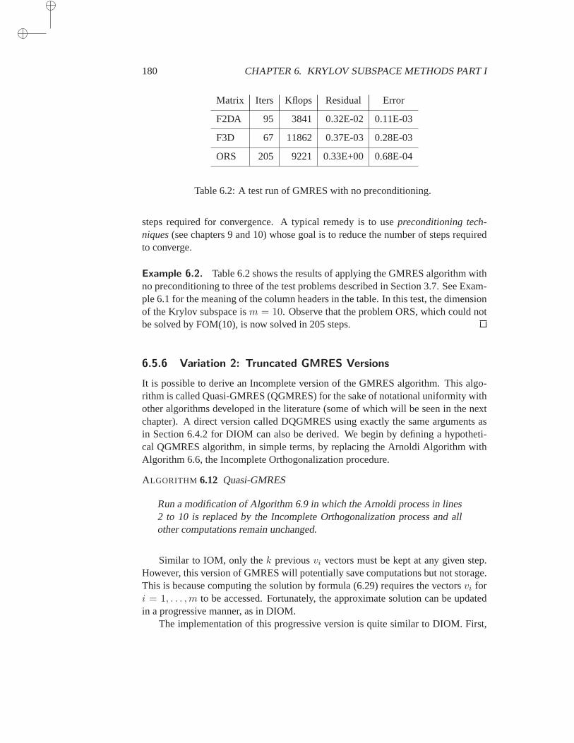
180 CHAPTER 6. KRYLOV SUBSPACE METHODS PART I
Matrix Iters Kflops Residual Error
F2DA 95 3841 0.32E-02 0.11E-03
F3D 67 11862 0.37E-03 0.28E-03
ORS 205 9221 0.33E+00 0.68E-04
Table 6.2: A test run of GMRES with no preconditioning.
steps required for convergence. A typical remedy is to usepreconditioning tech-niques(see chapters 9 and 10) whose goal is to reduce the number of steps requiredto converge.
Example 6.2. Table 6.2 shows the results of applying the GMRES algorithm withno preconditioning to three of the test problems described in Section 3.7. SeeExam-ple 6.1 for the meaning of the column headers in the table. In this test, the dimensionof the Krylov subspace ism = 10. Observe that the problem ORS, which could notbe solved by FOM(10), is now solved in 205 steps.
6.5.6 Variation 2: Truncated GMRES Versions
It is possible to derive an Incomplete version of the GMRES algorithm. This algo-rithm is called Quasi-GMRES (QGMRES) for the sake of notational uniformity withother algorithms developed in the literature (some of which will be seen in the nextchapter). A direct version called DQGMRES using exactly the same arguments asin Section 6.4.2 for DIOM can also be derived. We begin by defining a hypotheti-cal QGMRES algorithm, in simple terms, by replacing the Arnoldi Algorithm withAlgorithm 6.6, the Incomplete Orthogonalization procedure.
ALGORITHM 6.12 Quasi-GMRES
Run a modification of Algorithm 6.9 in which the Arnoldi process in lines2 to 10 is replaced by the Incomplete Orthogonalization process and allother computations remain unchanged.
Similar to IOM, only thek previousvi vectors must be kept at any given step.However, this version of GMRES will potentially save computations but not storage.This is because computing the solution by formula (6.29) requires the vectorsvi fori = 1, . . . ,m to be accessed. Fortunately, the approximate solution can be updatedin a progressive manner, as in DIOM.
The implementation of this progressive version is quite similar to DIOM. First,
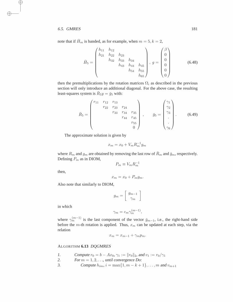
6.5. GMRES 181
note that ifHm is banded, as for example, whenm = 5, k = 2,
H5 =
h11 h12
h21 h22 h23
h32 h33 h34
h43 h44 h45
h54 h55
h65
, g =
β00000
(6.48)
then the premultiplications by the rotation matricesΩi as described in the previoussection will only introduce an additional diagonal. For the above case, the resultingleast-squares system isR5y = g5 with:
R5 =
r11 r12 r13r22 r23 r24
r33 r34 r35r44 r45
r550
, g5 =
γ1
γ2
γ3
.
.γ6
. (6.49)
The approximate solution is given by
xm = x0 + VmR−1m gm
whereRm andgm are obtained by removing the last row ofRm andgm, respectively.DefiningPm as in DIOM,
Pm ≡ VmR−1m
then,xm = x0 + Pmgm.
Also note that similarly to DIOM,
gm =
[gm−1
γm
]
in whichγm = cmγ
(m−1)m ,
whereγ(m−1)m is the last component of the vectorgm−1, i.e., the right-hand side
before them-th rotation is applied. Thus,xm can be updated at each step, via therelation
xm = xm−1 + γmpm.
ALGORITHM 6.13 DQGMRES
1. Computer0 = b−Ax0, γ1 := ‖r0‖2, andv1 := r0/γ1
2. Form = 1, 2, . . ., until convergence Do:3. Computehim, i = max1,m− k + 1, . . . ,m andvm+1
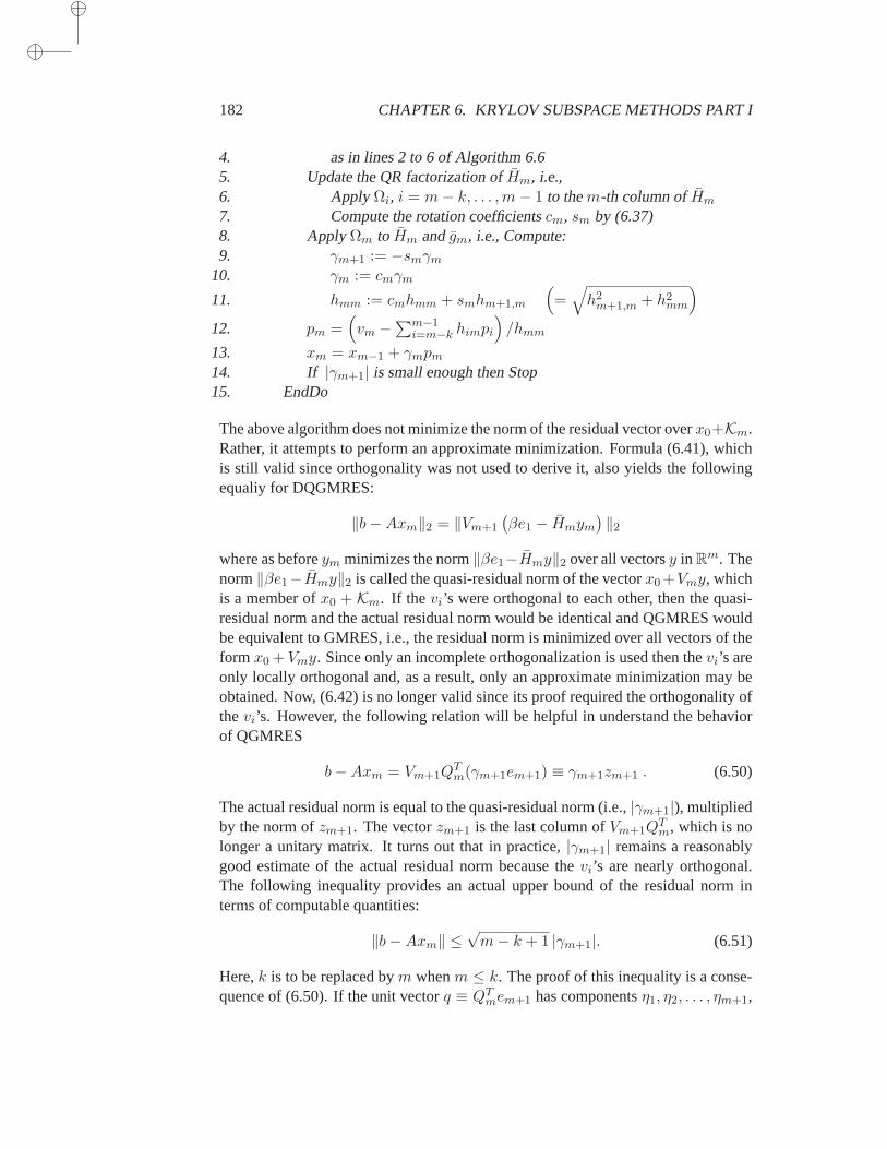
182 CHAPTER 6. KRYLOV SUBSPACE METHODS PART I
4. as in lines 2 to 6 of Algorithm 6.65. Update the QR factorization ofHm, i.e.,6. Apply Ωi, i = m− k, . . . ,m− 1 to them-th column ofHm
7. Compute the rotation coefficientscm, sm by (6.37)8. Apply Ωm to Hm andgm, i.e., Compute:9. γm+1 := −smγm
10. γm := cmγm
11. hmm := cmhmm + smhm+1,m
(
=√
h2m+1,m + h2
mm
)
12. pm =(
vm −∑m−1
i=m−k himpi
)
/hmm
13. xm = xm−1 + γmpm
14. If |γm+1| is small enough then Stop15. EndDo
The above algorithm does not minimize the norm of the residual vector overx0+Km.Rather, it attempts to perform an approximate minimization. Formula (6.41), whichis still valid since orthogonality was not used to derive it, also yields the followingequaliy for DQGMRES:
‖b−Axm‖2 = ‖Vm+1
(βe1 − Hmym
)‖2
where as beforeym minimizes the norm‖βe1−Hmy‖2 over all vectorsy in Rm. The
norm‖βe1−Hmy‖2 is called the quasi-residual norm of the vectorx0 +Vmy, whichis a member ofx0 + Km. If the vi’s were orthogonal to each other, then the quasi-residual norm and the actual residual norm would be identical and QGMRES wouldbe equivalent to GMRES, i.e., the residual norm is minimized over all vectors of theform x0 + Vmy. Since only an incomplete orthogonalization is used then thevi’s areonly locally orthogonal and, as a result, only an approximate minimization may beobtained. Now, (6.42) is no longer valid since its proof required the orthogonality ofthevi’s. However, the following relation will be helpful in understand the behaviorof QGMRES
b−Axm = Vm+1QTm(γm+1em+1) ≡ γm+1zm+1 . (6.50)
The actual residual norm is equal to the quasi-residual norm (i.e.,|γm+1|), multipliedby the norm ofzm+1. The vectorzm+1 is the last column ofVm+1Q
Tm, which is no
longer a unitary matrix. It turns out that in practice,|γm+1| remains a reasonablygood estimate of the actual residual norm because thevi’s are nearly orthogonal.The following inequality provides an actual upper bound of the residual norm interms of computable quantities:
‖b−Axm‖ ≤√m− k + 1 |γm+1|. (6.51)
Here,k is to be replaced bym whenm ≤ k. The proof of this inequality is a conse-quence of (6.50). If the unit vectorq ≡ QT
mem+1 has componentsη1, η2, . . . , ηm+1,
6.5. GMRES 183
then
‖b−Axm‖2 = |γm+1| ‖Vm+1q‖2
≤ |γm+1|
∥∥∥∥∥
k+1∑
i=1
ηivi
∥∥∥∥∥
2
+
∥∥∥∥∥
m+1∑
i=k+2
ηivi
∥∥∥∥∥
2
≤ |γm+1|
[k+1∑
i=1
η2i
]1/2
+
m+1∑
i=k+2
|ηi| ‖vi‖2
≤ |γm+1|
[k+1∑
i=1
η2i
]1/2
+√m− k
[m+1∑
i=k+2
η2i
]1/2
The orthogonality of the firstk+1 vectorsvi was used and the last term comes fromusing the Cauchy-Schwartz inequality. The desired inequality follows fromusing theCauchy-Schwartz inequality again in the form
1 . a+√m− k . b ≤
√m− k + 1
√
a2 + b2
and from the fact that the vectorq is of norm unity. Thus, using|γm+1| as a residualestimate, we would make an error of a factor of
√m− k + 1 at most. In general,
this is an overestimate and|γm+1| tends to give an adequate estimate for the residualnorm.
It is also interesting to observe that with a little bit more arithmetic, the exactresidual vector and norm can be obtained. This is based on the observation that,according to (6.50), the residual vector isγm+1 times the vectorzm+1 which is thelast column of the matrix
Zm+1 ≡ Vm+1QTm. (6.52)
It is an easy exercise to see that this last column can be updated fromvm+1 andzm.Indeed, assuming that all the matrices related to the rotation are of size(m + 1) ×(m + 1), the last row ofQm−1 is the(m + 1) − st row of the identity, so we canwrite
Zm+1 = [Vm, vm+1]QTm−1Ω
Tm
= [Zm, vm+1]ΩTm .
The result is thatzm+1 = −smzm + cmvm+1. (6.53)
Thezi’s can be updated at the cost of one extra vector in memory and4n operationsat each step. The norm ofzm+1 can be computed at the cost of2n operations andthe exact residual norm for the current approximate solution can then beobtained bymultiplying this norm by|γm+1|.
Because this is a little expensive, it may be preferred to just “correct” the estimateprovided byγm+1 by exploiting the above recurrence relation,
‖zm+1‖2 ≤ |sm|‖zm‖2 + |cm|.
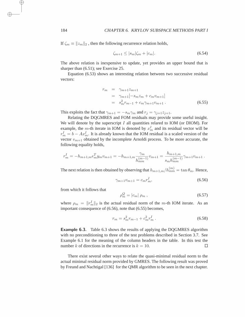
184 CHAPTER 6. KRYLOV SUBSPACE METHODS PART I
If ζm ≡ ‖zm‖2 , then the following recurrence relation holds,
ζm+1 ≤ |sm|ζm + |cm|. (6.54)
The above relation is inexpensive to update, yet provides an upper bound that issharper than (6.51); see Exercise 25.
Equation (6.53) shows an interesting relation between two successive residualvectors:
rm = γm+1zm+1
= γm+1[−smzm + cmvm+1]
= s2mrm−1 + cmγm+1vm+1 . (6.55)
This exploits the fact thatγm+1 = −smγm andrj = γj+1zj+1.Relating the DQGMRES and FOM residuals may provide some useful insight.
We will denote by the superscriptI all quantities relared to IOM (or DIOM). Forexample, them-th iterate in IOM is denoted byxI
m and its residual vector will berIm = b− AxI
m. It is already known that the IOM residual is a scaled version of thevectorvm+1 obtained by the incomplete Arnoldi process. To be more accurate, thefollowing equality holds,
rIm = −hm+1,me
Tmymvm+1 = −hm+1,m
γm
h(m−1)mm
vm+1 =hm+1,m
smh(m−1)mm
γm+1vm+1 .
The next relation is then obtained by observing thathm+1,m/h(m)mm = tan θm. Hence,
γm+1vm+1 = cmrIm, (6.56)
from which it follows thatρQ
m = |cm| ρm , (6.57)
whereρm = ‖rIm‖2 is the actual residual norm of them-th IOM iterate. As an
important consequence of (6.56), note that (6.55) becomes,
rm = s2mrm−1 + c2mrIm . (6.58)
Example 6.3. Table 6.3 shows the results of applying the DQGMRES algorithmwith no preconditioning to three of the test problems described in Section 3.7. SeeExample 6.1 for the meaning of the column headers in the table. In this test thenumberk of directions in the recurrence isk = 10.
There exist several other ways to relate the quasi-minimal residual norm totheactual minimal residual norm provided by GMRES. The following result wasprovedby Freund and Nachtigal [136] for the QMR algorithm to be seen in the nextchapter.
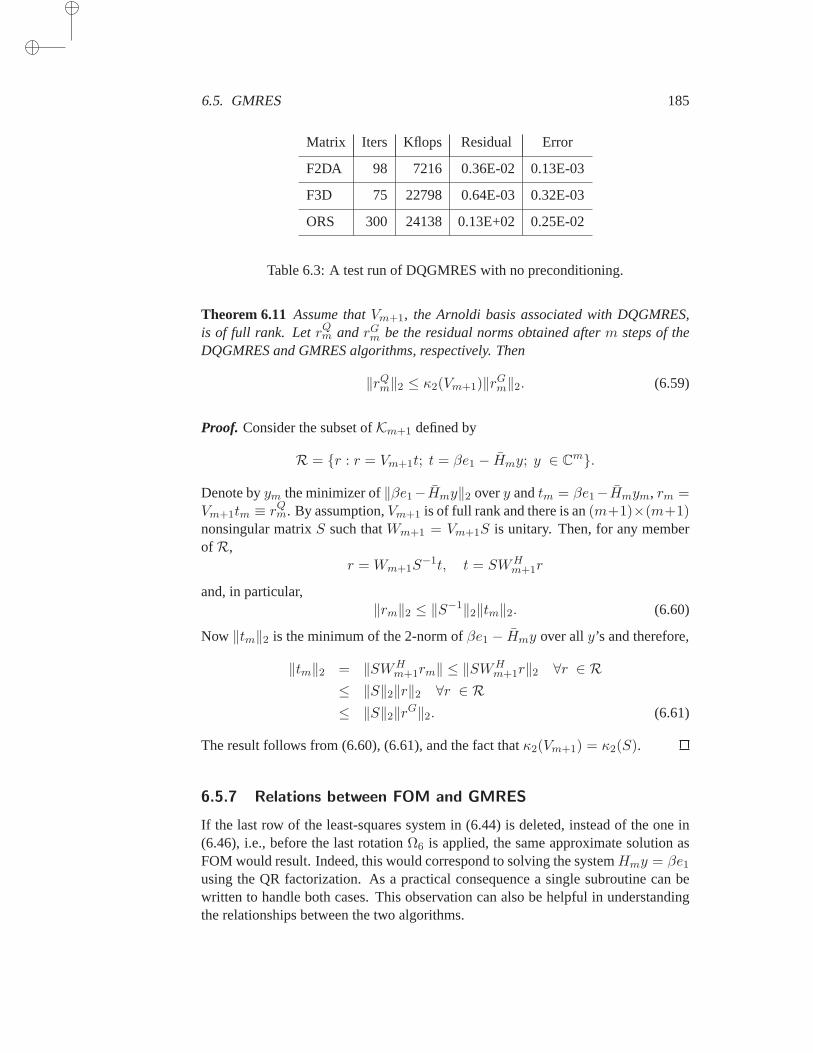
6.5. GMRES 185
Matrix Iters Kflops Residual Error
F2DA 98 7216 0.36E-02 0.13E-03
F3D 75 22798 0.64E-03 0.32E-03
ORS 300 24138 0.13E+02 0.25E-02
Table 6.3: A test run of DQGMRES with no preconditioning.
Theorem 6.11 Assume thatVm+1, the Arnoldi basis associated with DQGMRES,is of full rank. LetrQ
m and rGm be the residual norms obtained afterm steps of the
DQGMRES and GMRES algorithms, respectively. Then
‖rQm‖2 ≤ κ2(Vm+1)‖rG
m‖2. (6.59)
Proof. Consider the subset ofKm+1 defined by
R = r : r = Vm+1t; t = βe1 − Hmy; y ∈ Cm.
Denote byym the minimizer of‖βe1−Hmy‖2 overy andtm = βe1−Hmym, rm =Vm+1tm ≡ rQ
m. By assumption,Vm+1 is of full rank and there is an(m+1)×(m+1)nonsingular matrixS such thatWm+1 = Vm+1S is unitary. Then, for any memberofR,
r = Wm+1S−1t, t = SWH
m+1r
and, in particular,‖rm‖2 ≤ ‖S−1‖2‖tm‖2. (6.60)
Now ‖tm‖2 is the minimum of the 2-norm ofβe1 − Hmy over ally’s and therefore,
‖tm‖2 = ‖SWHm+1rm‖ ≤ ‖SWH
m+1r‖2 ∀r ∈ R≤ ‖S‖2‖r‖2 ∀r ∈ R≤ ‖S‖2‖rG‖2. (6.61)
The result follows from (6.60), (6.61), and the fact thatκ2(Vm+1) = κ2(S).
6.5.7 Relations between FOM and GMRES
If the last row of the least-squares system in (6.44) is deleted, instead of the one in(6.46), i.e., before the last rotationΩ6 is applied, the same approximate solution asFOM would result. Indeed, this would correspond to solving the systemHmy = βe1using the QR factorization. As a practical consequence a single subroutine can bewritten to handle both cases. This observation can also be helpful in understandingthe relationships between the two algorithms.
186 CHAPTER 6. KRYLOV SUBSPACE METHODS PART I
In what follows the FOM and GMRES iterates are denoted by the superscriptsF andG, respectively. The residual norm achieved at stepj will be denoted byρF
j
for FOM andρGj for GMRES. An important consequence of (6.47) is that
ρGm = |sm|ρG
m−1 ,
which leads to he following equality:
ρGm = |s1s2 . . . sm|β . (6.62)
Note that formulas (6.37) yield nonnegativesi’s, so the absolute values are not re-quired. They are left only for generality.
Define H(k)m to be the matrix resulting form applying the firstk rotations to
Hm and, similarly, letg(k)m be the vector resulting from applying the firstk rota-
tions to the right-hand sideβe1. As usualH(k)m is the matrixH(k)
m with its last rowdeleted andg(k)
m the vector of sizem obtained by removing the last component ofg(k)m . By formula (6.18), the residual obtained from the Arnoldi process is given
by ‖rFm‖2 = ‖b − AxF
m‖2 = hm+1,m|eTmym|. In addition,ym = H−1m (βe1) can
be obtained by back-solvingH(m−1)m y = g(m−1). Therefore, its last component is
eTmg(m−1)m /h
(m−1)mm . Hence,
ρFm = hm+1,m|eTmH−1
m (βe1)| = hm+1,m
∣∣∣∣∣
eTmg(m−1)
h(m−1)mm
∣∣∣∣∣.
As before, letγm denote the last component ofgm−1, or equivalently, them-th com-ponent ofg(m−1), i.e., before the last rotationΩm is applied (See (6.36) and (6.44)for an illustration). Then,
|eTmg(m−1)| = |sm−1γm| = · · · = |s1s2 . . . sm−1β| .
Therefore, the above expression forρFm becomes,
ρFm =
hm+1,m
|h(m−1)mm |
|s1s2 . . . sm−1β|.
Now expressions (6.37) show thathm+1,m/|h(m−1)mm | is the tangent of the angle defin-
ing them-th rotation, and therefore,
ρFm =
|sm||cm||s1s2 . . . sm−1β| .
A comparison with (6.62), yields a revealing relation between the residuals oftheFOM and GMRES algorithms, namely,
ρFm =
1
|cm|ρG
m .
The trigonometric relation1/ cos2 θ = 1 + tan2 θ, can now be invoked:1/|cm| =[1 + (hm+1,m/h
(m−1)mm )2]1/2. These results are summarized in the following propo-
sition (Brown [66]).
6.5. GMRES 187
Proposition 6.12 Assume thatm steps of the Arnoldi process have been taken andthatHm is nonsingular. Letξ ≡ (Qm−1Hm)mm andh ≡ hm+1,m. Then the residualnorms produced by the FOM and the GMRES algorithms are related by the equality
ρFm =
1
|cm|ρG
m = ρGm
√
1 +h2
ξ2. (6.63)
It is also possible to prove the above result by exploiting the relation (6.75);seeExercise 14.
The termξ in the expression (6.63) is not readily available and this results inan expression that is hard to interpret practically. Another, somewhat more explicitexpression, can be obtained from simply relatingcm with two consecutive residualnorms of GMRES. The next result shown by Cullum and Greenbaum [92]followsimmediatly from the above proposition and the relation|sm| = ρG
m/ρGm−1 which is a
consequence of (6.62).
Proposition 6.13 Assume thatm steps of the Arnoldi process have been taken andthat Hm is nonsingular. Then the residual norms produced by the FOM and theGMRES algorithms are related by the equality
ρFm =
ρGm
√
1−(ρG
m/ρGm−1
)2. (6.64)
The above relation can be recast as
1
(ρFm)2
+1
(ρG
m−1
)2 =1
(ρGm)2
(6.65)
Consider now these equations form,m− 1, · · ·, 1,
1
(ρFm)2
+1
(ρG
m−1
)2 =1
(ρGm)2
1(ρF
m−1
)2 +1
(ρG
m−2
)2 =1
(ρG
m−1
)2
· · · = · · ·1
(ρF1
)2 +1
(ρG0
)2 =1
(ρG1
)2
Note thatρG0 is simply the initial residual norm and can as well be denoted byρF
0 .Summing the above equations yields,
m∑
i=0
1(ρF
i
)2 =1
(ρGm)2
. (6.66)
188 CHAPTER 6. KRYLOV SUBSPACE METHODS PART I
Corollary 6.14 The residual norms produced by the FOM and the GMRES algo-rithms are related by the equality
ρGm =
1√∑m
i=0
(1/ρF
i
)2(6.67)
The above relation establishes rigorously the intuitive fact that FOM and GM-RES are never too far away from each other. It is clear thatρG
m ≤ ρFm. On the other
hand, letρFm∗
by the smallest residual norms achieved the firstm steps of FOM. Then
1
(ρGm)2
=m∑
i=0
1(ρF
i
)2 ≤m+ 1(ρF
m∗
)2
An immediate consequence of this inequality is the following proposition.
Proposition 6.15 Assume thatm steps of GMRES and FOM are taken (steps in FOMwith a singularHm are skipped). LetρF
m∗be the smallest residual norm achieved by
FOM in the firstm steps. Then, the following inequalities hold:
ρGm ≤ ρF
m∗≤ √m ρG
m (6.68)
We now establish another interesting relation between the FOM and GMRESiterates, which will be exploited in the next chapter. A general lemma is first shownregarding the solutions of the triangular systems
Rmym = gm
obtained from applying successive rotations to the Hessenberg matricesHm. As wasstated before, the only difference between theym vectors obtained in GMRES andArnoldi is that the last rotationΩm is omitted in FOM. In other words, theRm matrixfor the two methods differs only in its(m,m) entry while the right-hand sides differonly in their last components.
Lemma 6.16 Let Rm be them × m upper part of the matrixQm−1Hm and, asbefore, letRm be them ×m upper part of the matrixQmHm. Similarly, letgm bethe vector of the firstm components ofQm−1(βe1) and letgm be the vector of thefirstm components ofQm(βe1). Define
ym = R−1m gm, ym = R−1
m gm
the y vectors obtained for anm-dimensional FOM and GMRES methods, respec-tively. Then
ym −(ym−1
0
)
= c2m
(
ym −(ym−1
0
))
(6.69)
in whichcm is the cosine used in them-th rotationΩm, as defined by (6.37).

6.5. GMRES 189
Proof. The following relation holds:
Rm =
(Rm−1 zm
0 ξm
)
, Rm =
(Rm−1 zm
0 ξm
)
.
Similarly, for the right-hand sides,
gm =
(gm−1
γm
)
, gm =
(gm−1
γm
)
withγm = cmγm. (6.70)
Denoting byλ the scalar√
ξ2m + h2m+1,m, and using the definitions ofsm andcm,
we obtain
ξm = cmξm + smhm+1,m =ξ2mλ
+h2
m+1,m
λ= λ =
ξmcm. (6.71)
Now,
ym = R−1m gm =
(R−1
m−1 − 1ξmR−1
m−1zm0 1
ξm
)(gm−1
γm
)
(6.72)
which, upon observing thatR−1m−1gm−1 = ym−1, yields,
ym −(ym−1
0
)
=γm
ξm
(−R−1m−1zm1
)
. (6.73)
Replacingym, ξm, γm by ym, ξm, γm, respectively, in (6.72), a relation similar to(6.73) would result except thatγm/ξm is replaced byγm/ξm which, by (6.70) and(6.71), satisfies the relation
γm
ξm= c2m
γm
ξm.
The result follows immediately.
If the FOM and GMRES iterates are denoted by the superscriptsF andG, respec-tively, then the relation (6.69) implies that
xGm − xG
m−1 = c2m(xF
m − xGm−1
),
or,xG
m = s2mxGm−1 + c2mx
Fm. (6.74)
This leads to the following relation for the residual vectors obtained by the twometh-ods,
rGm = s2mr
Gm−1 + c2mr
Fm (6.75)
which indicates that, in general, the two residual vectors will evolve hand in hand.In particular, ifcm = 0, then GMRES will not progress at stepm, a phenomenonknown as stagnation. However, in this situation, according to the definitions (6.37)of the rotations,h(m−1)
mm = 0 which implies thatHm is singular and, therefore,xFm is
not defined. In fact, the reverse of this is also true, a result due to Brown [66], whichis stated without proof in the following proposition.
190 CHAPTER 6. KRYLOV SUBSPACE METHODS PART I
Proposition 6.17 If at any given stepm, the GMRES iterates make no progress, i.e.,if xG
m = xGm−1 thenHm is singular andxF
m is not defined. Conversely, ifHm issingular at stepm, i.e., if FOM breaks down at stepm, andA is nonsingular, thenxG
m = xGm−1.
Note also that the use of the above lemma is not restricted to the GMRES-FOMpair. Some of the iterative methods defined in this chapter and the next involvealeast-squares problem of the form (6.30). In such cases, the iterates of the least-squares method and those of the orthogonal residual (Galerkin) method will be re-lated by the same equation.
6.5.8 Residual smoothing
The previous section established strong relations between the GMRES and FOMiterates. In fact it is possible to derive the GMRES iterates from the FOM iterates,by simply exploiting the relations (6.74 – 6.75), which we now rewrite as
xGm = xG
m−1 + c2m(xFm − xG
m−1) ; rGm = rG
m−1 + c2m(rFm − rG
m−1) .
The above relations are instances of a class of algorithms derived by ‘residual smooth-ing’, which define a new sequence of iterates, denoted here byxS
i from an originalsequence, denoted byxO
i . The residual vectors of the two sequences are denoted byrSi andrO
i respectively. The new sequences are as follows:
xSm = xS
m−1 + ηm(xOm − xS
m−1) ; rSm = rS
m−1 + ηm(rOm − rS
m−1) .
The parameterηm is selected so as to make the residualrm behave better than theoriginal one, in the sense that large variations in the residual are dampened. In Min-imal Residual Smoothingthe ηm’s are selected to minimize the new residual norm‖rS
m‖2. This is in essence a minimal residual projection method in the directionxO
m − xSm−1 and it is achieved by selectingηm so that the new residualrS
m is orthog-onal toA(xO
m − xSm−1) = −(rO
m − rSm−1). Thus,
ηm = −(rSm−1, r
Om − rS
m−1)
‖rOm − rS
m−1‖22,
resulting in the following algorithm.
ALGORITHM 6.14 Minimal residual smoothing
1. xS0 = xO
0 , rS0 = rO
0 ;2. Form = 1, . . . , Do:3. ComputexO
m andrOm
4. ηm = −(rSm−1, r
Om − rS
m−1
)/‖rO
m − rSm−1‖22
5. xSm = xS
m−1 + ηm(xOm − xS
m−1)6. rS
m = rSm−1 + ηm(rO
m − rSm−1)
7. EndDo

6.5. GMRES 191
In the situation whenrOm is orthogonal torS
m−1, then it is possible to show that thesame relation as (6.64) (or equivalently (6.65)) is satisfied. This result is due toWeiss [307].
Lemma 6.18 If rOm is orthogonal torS
m−1 at each stepm ≥ 1, then the residualnorms satisfy the relation
1
‖rSm‖22
=1
‖rSm−1‖22
+1
‖rOm‖22
, (6.76)
and the coefficientηm is given by
ηm =‖rS
m−1‖22‖rS
m−1‖22 + ‖rOm‖22
. (6.77)
Proof. SincerOm ⊥ rS
m−1 it follows that(rSm−1, r
Om − rS
m−1) = −(rSm−1, r
Sm−1) and
‖rOm − rS
m−1‖22 = ‖rOm‖22 + ‖rS
m−1‖22. This shows (6.77). The orthogonality ofrSm
with rSm − rS
m−1, implies that
‖rSm‖22 = ‖rS
m−1‖22 − η2m‖rO
m − rSm−1‖22
= ‖rSm−1‖22 −
‖rSm−1‖42
‖rOm‖22 + ‖rS
m−1‖22=‖rS
m−1‖2‖rOm‖22
‖rOm‖22 + ‖rS
m−1‖22.
The result (6.76) follows by inverting both sides of the above equality.
The assumptions of the lemma are satisfied in particular when the residual vec-tors of the original algorithm are orthogonal to each other, as is the case for the FOMmethod. This can be shown by simple induction, using the fact that each newrS
k isultimately a linear combination of therO
i ’s, for i ≤ k. Since the relation establishedby the lemma is identical with that of the GMRES algorithm, it follows that theresidual norms are identical, since they both satisfy (6.67). Because the approximatesolutions belong to the same subspace and GMRES minimizes the residual norm, itis clear thatthe resulting approximate solutions are identical.
This result can also be shown in a different way. Induction shows that the vectorspj = xO
j − xSj−1 areATA - orthogonal, i.e.,(Api, Apj) = 0 for i 6=. Then a lemma
to be seen in Section 6.9 (Lemma 6.21) can be expoited to prove the same result.This is left as an exercise (Exercise 26).
The computation of the scalarηm is likely to be subject to large errors whenthe residuals become small because there may be a substantial difference betweenthe actual residual and the one computed recursively by the algorithm. Oneremedyis to explicitly use the directionspj mentioned above. The formulas and the actualupdate will then follow closely those seen in Section 5.3, withv replaced bypm,andw by Apm. Speficially, lines 5 and 6 of Algorithm 6.14 are repaced byxS
m =xS
m−1 + ηmpm andrSm = rS
m−1 − ηmApm, respectively, while the coefficientηm
is computed asηm = (rSm−1, Apm)/(Apm, Apm). Details are omitted but may be
found in [324].
192 CHAPTER 6. KRYLOV SUBSPACE METHODS PART I
Lemma 6.18 yields the following equality, in whichρj denotes‖rOj ‖2 andτj
denotes‖rSj ‖2,
rSm =
ρ2m
ρ2m + τ2
m−1
rSm−1 +
τ2m−1
ρ2m + τ2
m−1
rOm
=1
1τ2m−1
+ 1ρ2
m
[1
τ2m−1
rSm−1 +
1
ρ2m
rOm
]
. (6.78)
Summing up the relations (6.76), yields an expression similar to (6.66),
1
τ2j
=
j∑
i=0
1
ρ2j
.
Combining this with (6.78) and using induction immediatly yields the following ex-pression which holds under the assumptions of Lemma 6.18 :
rSm =
1∑m
j=11ρ2
j
m∑
j=1
rOj
ρ2j
. (6.79)
The smoothed residual is a convex combination of the residuals obtained by the orig-inal algorithm (e.g., FOM). The coefficient used for a given residual isinverselyproportional to its norm squared. In other words, residual smoothing willtend todampen wide variations in the original residuals. If the original residual moves upvery high then (6.79) or (6.78) show that the next S-residual will tend to stagnate. Ifthe other hand, the original residual decreases very rapidly at a given step, then thesmoothed residual will be close to it. In other words, stagnation and fast convergenceof the S-residual goes hand in hand with poor convergence and fast convergence, re-spectively, of the original scheme.
Consider now the general situation when the residual vectors do not satisfy theconditions of Lemma 6.18. In this case the above results are not valid. However,one may ask whether or not it is possible to still select theηm’s by an alternativeformula such that the nice relation (6.79) remains valid. A hint at a possible answeris provided by a look at Equations (6.76) and (6.77). These are the only relationsused to establish (6.79). This suggests computing theηm’s recursively as follows
ηm =τ2m−1
τ2m−1 + ρ2
m
;1
τ2m
=1
τ2m−1
+1
ρ2m
It is only when the conditions of Lemma 6.18 are satisfied, thatτk is the norm of theresidualsrS
k . What is important is that the relation (6.78) can be shown to be validwith ‖rS
j ‖22 replaced byτ2j . As result, the same induction proof as before will show
that (6.79) is also valid. Replacing theηm of Algorithm 6.14 by the one defined abovegives rise to an algorithm known asquasi-minimal residual smoothing, or QMRS.
It can easily be shown that when applied to the sequence of iterates producedby IOM/DIOM, then QMRS will, in exact arithmetic, yield the same sequence as
6.5. GMRES 193
QMRES/DQGMRES. The key relations are (6.47), which is still valid, and (6.57).The quasi-residual norm which replaces the actual normrS
m is now equal toγm+1.By (6.57), the cosine used in them-th step of QGMRES/DQGMES satisfies:|cm| =|γm+1|/ρ2
m. By formula (6.47),|sm| = |γm+1/γm|. Writing c2m + s2m = 1 and usingthe notationτm ≡ γm+1, yields
γ2m+1
γ2m
+γ2
m+1
ρ2m
= 1 → 1
τ2m
=1
τ2m−1
+1
ρ2m
This, along with the relation (6.58), shows that the residual vectors computed byQGMRES-/DQGMRES obey the exact same recurrence as those defined by QMRS.Quasi-minimal residual smoothing is related to several other algorithms to be de-scribed in the next sections.
6.5.9 GMRES for complex systems
Complex linear systems arise in many important applications. Perhaps the bestknown of these is when solving Maxwell’s equations in electromagnetics. Themostcommon method used in this context gives rise to large dense and complex linearsystems.
Adapting GMRES to the complex case is fairly straightforward. The guidingprinciple is that the method should minimize the 2-norm of the residual on the affineKrylov subspace. This is achieved by Algorithm 6.9 in which the inner products arenow the complex inner produts inCn, defined by (1.3) of Chapter 1. The only partrequiring some attention is the solution of the least-squares problem in Line 12 of theAlgorithm or rather, the practical implementation using Givens rotations outlinedinSection 6.5.3.
Complex Givens rotations are defined in the following way instead of (6.34):
Ωi =
1. . .
1ci si
−si ci1
.. .1
← row i← row i+ 1
(6.80)
with |ci|2 + |si|2 = 1. The description of Section 6.5.3 can be followed in the sameway. In particular the sine and cosine defined in (6.37) for the Givens rotation matrixat stepi are given by
si =hi+1,i
√
|h(i−1)ii |2 + h2
i+1,i
, ci =h
(i−1)ii
√
|h(i−1)ii |2 + h2
i+1,i
. (6.81)
A slight simplification takes place when applying the successive rotations. Sincehj+1,j is the 2-norm of a vector, it is real (nonnegative), and sosi is also a real
194 CHAPTER 6. KRYLOV SUBSPACE METHODS PART I
(nonnegative) number while, in general,ci is complex. The rest of the developmentis identical, though it is worth noting that the diagonal entries of the upper triangularmatrixR are (nonnegative) real and that the scalarsγi are real.
6.6 The Symmetric Lanczos Algorithm
The symmetric Lanczos algorithm can be viewed as a simplification of Arnoldi’smethod for the particular case when the matrix is symmetric. WhenA is symmetric,then the Hessenberg matrixHm becomes symmetric tridiagonal. This leads to athree-term recurrence in the Arnoldi process and short-term recurrences for solutionalgorithms such as FOM and GMRES. On the theoretical side, there is also muchmore that can be said on the resulting approximation in the symmetric case.
6.6.1 The Algorithm
To introduce the Lanczos algorithm we begin by making the observation statedin thefollowing theorem.
Theorem 6.19 Assume that Arnoldi’s method is applied to a real symmetric matrixA. Then the coefficientshij generated by the algorithm are such that
hij = 0, for 1 ≤ i < j − 1, (6.82)
hj,j+1 = hj+1,j , j = 1, 2, . . . ,m. (6.83)
In other words, the matrixHm obtained from the Arnoldi process is tridiagonal andsymmetric.
Proof. The proof is an immediate consequence of the fact thatHm = V TmAVm is
a symmetric matrix which is also a Hessenberg matrix by construction. Therefore,Hm must be a symmetric tridiagonal matrix.
The standard notation used to describe the Lanczos algorithm is obtained bysetting
αj ≡ hjj , βj ≡ hj−1,j ,
and ifTm denotes the resultingHm matrix, it is of the form,
Tm =
α1 β2
β2 α2 β3
. . .βm−1 αm−1 βm
βm αm
. (6.84)
This leads to the following form of the Modified Gram-Schmidt variant of Arnoldi’smethod, namely, Algorithm 6.2.
ALGORITHM 6.15 The Lanczos Algorithm
6.6. THE SYMMETRIC LANCZOS ALGORITHM 195
1. Choose an initial vectorv1 of 2-norm unity. Setβ1 ≡ 0, v0 ≡ 02. Forj = 1, 2, . . . ,m Do:3. wj := Avj − βjvj−1
4. αj := (wj , vj)5. wj := wj − αjvj
6. βj+1 := ‖wj‖2. If βj+1 = 0 then Stop7. vj+1 := wj/βj+1
8. EndDo
It is rather surprising that the above simple algorithm guarantees, at leastin exactarithmetic, that the vectorsvi, i = 1, 2, . . . , are orthogonal. In reality, exact orthogo-nality of these vectors is only observed at the beginning of the process. At some pointthevi’s start losing their global orthogonality rapidly. There has been much researchdevoted to finding ways to either recover the orthogonality, or to at least diminish itseffects bypartial or selectiveorthogonalization; see Parlett [224].
The major practical differences with Arnoldi’s method are that the matrixHm istridiagonal and, more importantly, that only three vectors must be saved, unless someform of reorthogonalization is employed.
6.6.2 Relation with Orthogonal Polynomials
In exact arithmetic, the core of Algorithm 6.15 is a relation of the form
βj+1vj+1 = Avj − αjvj − βjvj−1.
This three-term recurrence relation is reminiscent of the standard three-term recur-rence relation of orthogonal polynomials. In fact, there is indeed a strongrelationshipbetween the Lanczos algorithm and orthogonal polynomials. To begin, recall that ifthe grade ofv1 is≥ m, then the subspaceKm is of dimensionm and consists of allvectors of the formq(A)v1, whereq is a polynomial withdegree(q) ≤ m−1. In thiscase there is even an isomorphism betweenKm andPm−1, the space of polynomialsof degree≤ m− 1, which is defined by
q ∈ Pm−1 → x = q(A)v1 ∈ Km.
Moreover, we can consider that the subspacePm−1 is provided with the inner product
< p, q >v1= (p(A)v1, q(A)v1). (6.85)
This is indeed a nondegenerate bilinear form under the assumption thatm does notexceedµ, the grade ofv1. Now observe that the vectorsvi are of the form
vi = qi−1(A)v1
and the orthogonality of thevi’s translates into the orthogonality of the polynomialswith respect to the inner product (6.85).
196 CHAPTER 6. KRYLOV SUBSPACE METHODS PART I
It is known that real orthogonal polynomials satisfy a three-term recurrence.Moreover, the Lanczos procedure is nothing but the Stieltjes algorithm; (see, forexample, Gautschi [141]) for computing a sequence of orthogonal polynomials withrespect to the inner product (6.85). It is known [246] that the characteristic poly-nomial of the tridiagonal matrix produced by the Lanczos algorithm minimizes thenorm‖.‖v1 over the monic polynomials. The recurrence relation between the char-acteristic polynomials of tridiagonal matrices also shows that the Lanczos recurrencecomputes the sequence of vectorspTm(A)v1, wherepTm is the characteristic polyno-mial of Tm.
6.7 The Conjugate Gradient Algorithm
The Conjugate Gradient algorithm is one of the best known iterative techniques forsolving sparse Symmetric Positive Definite linear systems. Described in one sen-tence, the method is a realization of an orthogonal projection technique onto theKrylov subspaceKm(r0, A) wherer0 is the initial residual. It is therefore mathemat-ically equivalent to FOM. However, becauseA is symmetric, some simplificationsresulting from the three-term Lanczos recurrence will lead to more elegant algo-rithms.
6.7.1 Derivation and Theory
We first derive the analogue of FOM, or Arnoldi’s method, for the case whenA issymmetric. Given an initial guessx0 to the linear systemAx = b and the Lanczosvectorsvi, i = 1, . . . ,m together with the tridiagonal matrixTm, the approximatesolution obtained from an orthogonal projection method ontoKm, is given by
xm = x0 + Vmym, ym = T−1m (βe1). (6.86)
ALGORITHM 6.16 Lanczos Method for Linear Systems
1. Computer0 = b−Ax0, β := ‖r0‖2, andv1 := r0/β2. Forj = 1, 2, . . . ,m Do:3. wj = Avj − βjvj−1 (If j = 1 setβ1v0 ≡ 0)4. αj = (wj , vj)5. wj := wj − αjvj
6. βj+1 = ‖wj‖2. If βj+1 = 0 setm := j and go to 97. vj+1 = wj/βj+1
8. EndDo9. SetTm = tridiag (βi, αi, βi+1), andVm = [v1, . . . , vm].
10. Computeym = T−1m (βe1) andxm = x0 + Vmym
Many of the results obtained from Arnoldi’s method for linear systems are stillvalid.For example, the residual vector of the approximate solutionxm is such that
b−Axm = −βm+1eTmymvm+1. (6.87)

6.7. THE CONJUGATE GRADIENT ALGORITHM 197
The Conjugate Gradient algorithm can be derived from the Lanczos algorithm inthe same way DIOM was derived from IOM. In fact, the Conjugate Gradient algo-rithm can be viewed as a variation of DIOM(2) for the case whenA is symmetric. Wewill follow the same steps as with DIOM, except that the notation will be simplifiedwhenever possible.
First write the LU factorization ofTm asTm = LmUm. The matrixLm is unitlower bidiagonal andUm is upper bidiagonal. Thus, the factorization ofTm is of theform
Tm =
1λ2 1
λ3 1λ4 1
λ5 1
×
η1 β2
η2 β3
η3 β4
η4 β5
η5
.
The approximate solution is then given by,
xm = x0 + VmU−1m L−1
m (βe1).
LettingPm ≡ VmU
−1m
andzm = L−1
m βe1,
then,xm = x0 + Pmzm.
As for DIOM, pm, the last column ofPm, can be computed from the previouspi’sandvm by the simple update
pm = η−1m [vm − βmpm−1].
Note thatβm is a scalar computed from the Lanczos algorithm, whileηm results fromthem-th Gaussian elimination step on the tridiagonal matrix, i.e.,
λm =βm
ηm−1, (6.88)
ηm = αm − λmβm. (6.89)
In addition, following again what has been shown for DIOM,
zm =
[zm−1
ζm
]
,
in which ζm = −λmζm−1. As a result,xm can be updated at each step as
xm = xm−1 + ζmpm
wherepm is defined above.This gives the following algorithm, which we call the direct version of the Lanc-
zos algorithm for linear systems.
198 CHAPTER 6. KRYLOV SUBSPACE METHODS PART I
ALGORITHM 6.17 D-Lanczos
1. Computer0 = b−Ax0, ζ1 := β := ‖r0‖2, andv1 := r0/β2. Setλ1 = β1 = 0, p0 = 03. Form = 1, 2, . . ., until convergence Do:4. Computew := Avm − βmvm−1 andαm = (w, vm)
5. If m > 1 then computeλm = βm
ηm−1andζm = −λmζm−1
6. ηm = αm − λmβm
7. pm = η−1m (vm − βmpm−1)
8. xm = xm−1 + ζmpm
9. If xm has converged then Stop10. w := w − αmvm
11. βm+1 = ‖w‖2, vm+1 = w/βm+1
12. EndDo
This algorithm computes the solution of the tridiagonal systemTmym = βe1progressively by using Gaussian elimination without pivoting. However, as was ex-plained for DIOM, partial pivoting can also be implemented at the cost of having tokeep an extra vector. In fact, Gaussian elimination with partial pivoting is sufficientto ensure stability for tridiagonal systems. The more complex LQ factorization hasalso been exploited in this context and gave rise to an algorithm known as SYMMLQ[223].
The two algorithms 6.16 and 6.17 are mathematically equivalent, that is, theydeliver the same approximate solution if they are both executable. However,sinceGaussian elimination without pivoting is being used implicitly to solve the tridiago-nal systemTmy = βe1, the direct version may be more prone to breakdowns.
Observe that the residual vector for this algorithm is in the direction ofvm+1 dueto equation (6.87). Therefore, the residual vectors are orthogonal toeach other asin FOM. Likewise, the vectorspi areA-orthogonal, orconjugate. These results areestablished in the next proposition.
Proposition 6.20 Letrm = b−Axm,m = 0, 1, . . ., be the residual vectors producedby the Lanczos and the D-Lanczos algorithms (6.16 and 6.17) andpm,m = 0, 1, . . . ,the auxiliary vectors produced by Algorithm 6.17. Then,
1. Each residual vectorrm is such thatrm = σmvm+1 whereσm is a certainscalar. As a result, the residual vectors are orthogonal to each other.
2. The auxiliary vectorspi form anA-conjugate set, i.e.,(Api, pj) = 0, for i 6= j.
Proof. The first part of the proposition is an immediate consequence of the relation(6.87). For the second part, it must be proved thatP T
mAPm is a diagonal matrix,wherePm = VmU
−1m . This follows from
P TmAPm = U−T
m V TmAVmU
−1m
= U−Tm TmU
−1m
= U−Tm Lm.
6.7. THE CONJUGATE GRADIENT ALGORITHM 199
Now observe thatU−Tm Lm is a lower triangular matrix which is also symmetric since
it is equal to the symmetric matrixP TmAPm. Therefore, it must be a diagonal matrix.
A consequence of the above proposition is that a version of the algorithm can bederived by imposing the orthogonality and conjugacy conditions. This gives the Con-jugate Gradient algorithm which we now derive. The vectorxj+1 can be expressedas
xj+1 = xj + αjpj . (6.90)
In order to conform with standard notation used in the literature to describe the algo-rithm, the indexing of thep vectors now begins at zero instead of one as was done sofar. This explains the difference between the above formula and formula (6.21) usedfor DIOM. Now, the residual vectors must satisfy the recurrence
rj+1 = rj − αjApj . (6.91)
If the rj ’s are to be orthogonal, then it is necessary that(rj − αjApj , rj) = 0 and asa result
αj =(rj , rj)
(Apj , rj). (6.92)
Also, it is known that the next search directionpj+1 is a linear combination ofrj+1
andpj , and after rescaling thep vectors appropriately, it follows that
pj+1 = rj+1 + βjpj . (6.93)
Thus, a first consequence of the above relation is that
(Apj , rj) = (Apj , pj − βj−1pj−1) = (Apj , pj)
becauseApj is orthogonal topj−1. Then, (6.92) becomesαj = (rj , rj)/(Apj , pj).In addition, writing thatpj+1 as defined by (6.93) is orthogonal toApj yields
βj = −(rj+1, Apj)
(pj , Apj).
Note that from (6.91)
Apj = − 1
αj(rj+1 − rj) (6.94)
and therefore,
βj =1
αj
(rj+1, (rj+1 − rj))(Apj , pj)
=(rj+1, rj+1)
(rj , rj).
Putting these relations together gives the following algorithm.
ALGORITHM 6.18 Conjugate Gradient
200 CHAPTER 6. KRYLOV SUBSPACE METHODS PART I
1. Computer0 := b−Ax0, p0 := r0.2. Forj = 0, 1, . . ., until convergence Do:3. αj := (rj , rj)/(Apj , pj)4. xj+1 := xj + αjpj
5. rj+1 := rj − αjApj
6. βj := (rj+1, rj+1)/(rj , rj)7. pj+1 := rj+1 + βjpj
8. EndDo
It is important to note that the scalarsαj , βj in this algorithm are different from thoseof the Lanczos algorithm. The vectorspj are multiples of thepj ’s of Algorithm 6.17.In terms of storage, in addition to the matrixA, four vectors (x, p,Ap, andr) must besaved in Algorithm 6.18, versus five vectors (vm, vm−1, w, p, andx) for Algorithm6.17.
6.7.2 Alternative Formulations
Algorithm 6.18 is the best known formulation of the Conjugate Gradient algorithm.There are, however, several alternative formulations. Here, only one such formula-tion is shown, which can be derived once more from the Lanczos algorithm.
The residual polynomialrm(t) associated with them-th CG iterate must satisfya three-term recurrence, implied by the three-term recurrence of the Lanczos vectors.Indeed, these vectors are just the scaled versions of the residual vectors. Therefore,we must seek a three-term recurrence of the form
rm+1(t) = ρm(rm(t)− γmtrm(t)) + δmrm−1(t).
In addition, the consistency conditionrm(0) = 1 must be maintained for eachm,leading to the recurrence,
rm+1(t) = ρm(rm(t)− γmtrm(t)) + (1− ρm)rm−1(t). (6.95)
Observe that ifrm(0) = 1 andrm−1(0) = 1, thenrm+1(0) = 1, as desired. Trans-lating the above relation into the sequence of residual vectors yields
rm+1 = ρm(rm − γmArm) + (1− ρm)rm−1. (6.96)
Recall that the vectorsri’s are multiples of the Lanczos vectorsvi’s. As a result,γm should be the inverse of the scalarαm of the Lanczos algorithm. In terms of ther-vectors this means
γm =(rm, rm)
(Arm, rm).
Equating the inner products of both sides of (6.96) withrm−1, and using the orthog-onality of ther-vectors, gives the following expression forρm, after some algebraiccalculations,
ρm =
[
1− γm
γm−1
(rm, rm)
(rm−1, rm−1)
1
ρm−1
]−1
. (6.97)
6.7. THE CONJUGATE GRADIENT ALGORITHM 201
The recurrence relation for the approximate solution vectors can be extractedfrom the recurrence relation for the residual vectors. This is found bystarting from(6.95) and using the relationrm(t) = 1− tsm−1(t) between the solution polynomialsm−1(t) and the residual polynomialrm(t). Thus,
sm(t) =1− rm+1(t)
t
= ρm
(1− rm(t)
t− γmrm(t)
)
+ (1− ρm)1− rm−1(t)
t
= ρm (sm−1(t)− γmrm(t)) + (1− ρm)sm−2(t).
This gives the recurrence,
xm+1 = ρm(xm − γmrm) + (1− ρm)xm−1. (6.98)
All that is left for the recurrence to be determined completely is to define the firsttwo iterates. The initial iteratex0 is given. The first vector should be of the form
x1 = x0 − γ0r0,
to ensure thatr1 is orthogonal tor0. This means that the two-term recurrence can bestarted withρ0 = 1, and by settingx−1 ≡ 0. Putting these relations and definitionstogether gives the following algorithm.
ALGORITHM 6.19 CG – Three-Term Recurrence Variant
1. Computer0 = b−Ax0. Setx−1 ≡ 0 andρ0 = 1.2. Forj = 0, 1, . . ., until convergence Do:
3. ComputeArj andγj =(rj ,rj)
(Arj ,rj)
4. If (j > 0) computeρj =[
1− γj
γj−1
(rj ,rj)(rj−1,rj−1)
1ρj−1
]−1
5. Compute xj+1 = ρj (xj − γjrj) + (1− ρj)xj−1
6. Compute rj+1 = ρj(rj − γjArj) + (1− ρj)rj−1
7. EndDo
This algorithm requires slightly more storage than the standard formulation: in addi-tion toA, the vectorsrj , Arj , rj−1, xj andxj−1 must be kept. It is possible to avoidkeepingrj−1 by computing the residualrj+1 directly asrj+1 = b−Axj+1 in line 6of the algorithm, but this would entail an additional matrix-vector product.
6.7.3 Eigenvalue Estimates from the CG Coefficients
Sometimes, it is useful to be able to obtain the tridiagonal matrixTm related to theunderlying Lanczos iteration from the coefficients of the Conjugate Gradient algo-rithm 6.18. This tridiagonal matrix can provide valuable eigenvalue informationonthe matrixA. For example, the largest and smallest eigenvalues of the tridiagonalmatrix can approximate the smallest and largest eigenvalues ofA. This could be
202 CHAPTER 6. KRYLOV SUBSPACE METHODS PART I
used to compute an estimate of the condition number ofA which in turn can helpprovide estimates of the error norm from the residual norm. Since the Greek lettersαi andβi have been used in both algorithms, notations must be changed. Denote by
Tm = tridiag [ηj , δj , ηj+1],
the tridiagonal matrix (6.84) associated with them-th step of the Lanczos algorithm.We must seek expressions of the coefficientsηj , δj in terms of the coefficientsαj , βj ,obtained from the CG algorithm. The key information regarding the correspondencebetween the two pairs of coefficients resides in the correspondence between the vec-tors generated by the two algorithms.
From (6.87) it is known that
rj = scalar× vj+1. (6.99)
As a result,
δj+1 =(Avj+1, vj+1)
(vj+1, vj+1)=
(Arj , rj)
(rj , rj).
The denominator(rj , rj) is readily available from the coefficients of the CG algo-rithm, but the numerator(Arj , rj) is not. The relation (6.93) can be exploited toobtain
rj = pj − βj−1pj−1 (6.100)
which is then substituted in(Arj , rj) to get
(Arj , rj) = (A(pj − βj−1pj−1), pj − βj−1pj−1) .
Note that the termsβj−1pj−1 are defined to be zero whenj = 0. Because thepvectors areA-orthogonal,
(Arj , rj) = (Apj , pj) + β2j−1 (Apj−1, pj−1) ,
from which we finally obtain forj > 0,
δj+1 =(Apj , pj)
(rj , rj)+ β2
j−1
(Apj−1, pj−1)
(rj , rj)=
1
αj+βj−1
αj−1. (6.101)
The above expression is only valid forj > 0. For j = 0, the second term in theright-hand side should be omitted as was observed above. Therefore, the diagonalelements ofTm are given by
δj+1 =
1αj
for j = 0,
1αj
+βj−1
αj−1for j > 0.
(6.102)
Now an expression for the co-diagonal elementsηj+1 is needed. From the defi-nitions in the Lanczos algorithm,
ηj+1 = (Avj , vj+1) =|(Arj−1, rj)|‖rj−1‖2‖rj‖2
.
6.8. THE CONJUGATE RESIDUAL METHOD 203
Using (6.100) again and the relation (6.94) as well as orthogonality properties of theCG algorithm, the following sequence of equalities results:
(Arj−1, rj) = (A(pj−1 − βj−2pj−2), rj)
= (Apj−1, rj)− βj−2(Apj−2, rj)
=−1
αj−1(rj − rj−1, rj) +
βj−2
αj−2(rj−1 − rj−2, rj)
=−1
αj−1(rj , rj).
Therefore,
ηj+1 =1
αj−1
(rj , rj)
‖rj−1‖2‖rj‖2=
1
αj−1
‖rj‖2‖rj−1‖2
=
√βj−1
αj−1.
This finally gives the general form of them-dimensional Lanczos tridiagonal matrixin terms of the CG coefficients,
Tm =
1α0
√β0
α0√β0
α0
1α1
+ β0
α0
√β1
α1
. . .
. .
√βm−2
αm−2√βm−2
αm−2
1αm−1
+ βm−2
αm−2
. (6.103)
6.8 The Conjugate Residual Method
In the previous section we derived the Conjugate Gradient algorithm as a specialcase of FOM for Symmetric Positive Definite matrices. Similarly, a new algorithmcan be derived from GMRES for the particular case whereA is Hermitian. In thiscase, the residual vectors should beA-orthogonal, i.e., conjugate. In addition, thevectorsApi’s i = 0, 1, . . . , are orthogonal. When looking for an algorithm with thesame structure as CG, but satisfying these conditions, we find the Conjugate Residualalgorithm. Notice that the residual vectors are now conjugate to each other,hence,the name of the algorithm.
ALGORITHM 6.20 Conjugate Residual Algorithm
1. Computer0 := b−Ax0, p0 := r02. Forj = 0, 1, . . . , until convergence Do:3. αj := (rj , Arj)/(Apj , Apj)4. xj+1 := xj + αjpj
5. rj+1 := rj − αjApj
6. βj := (rj+1, Arj+1)/(rj , Arj)7. pj+1 := rj+1 + βjpj
8. ComputeApj+1 = Arj+1 + βjApj
9. EndDo
204 CHAPTER 6. KRYLOV SUBSPACE METHODS PART I
Line 8 in the above algorithm computesApj+1 from Arj+1 without an additionalmatrix-vector product. Five vectors of storage are needed in addition to the matrixA:x, p,Ap, r,Ar. The algorithm requires one more vector update, i.e.,2n more opera-tions than the Conjugate Gradient method and one more vector of storage. Since thetwo methods exhibit typically similar convergence, the Conjugate Gradient methodis often preferred.
6.9 GCR, ORTHOMIN, and ORTHODIR
All algorithms developed in this chapter are strongly related to, as well as definedby, the choice of a basis of the Krylov subspace. The GMRES algorithm uses an or-thonormal basis. In the Conjugate Gradient algorithm, thep’s areA-orthogonal, i.e.,conjugate. In the Conjugate Residual method just described, theApi’s are orthog-onal, i.e., thepi’s areATA-orthogonal. A number of algorithms can be developedusing a basis of this form in the nonsymmetric case as well. The main result that isexploited in all these algorithms is the following lemma.
Lemma 6.21 Letp0, p1, . . . , pm−1, be a sequence of vectors such that each setp0, p1,-. . . , pj−1 for j ≤ m is a basis of the Krylov subspaceKj(A, r0) which isATA-orthogonal, i.e., such that
(Api, Apk) = 0, for i 6= k.
Then the approximate solutionxm which has the smallest residual norm in the affinespacex0 +Km(A, r0) is given by
xm = x0 +m−1∑
i=0
(r0, Api)
(Api, Api)pi. (6.104)
In addition,xm can be computed fromxm−1 by
xm = xm−1 +(rm−1, Apm−1)
(Apm−1, Apm−1)pm−1. (6.105)
Proof. The approximate solution and the associated residual vector can be written inthe form
xm = x0 +m−1∑
i=0
αipi, rm = r0 −m−1∑
i=0
αiApi. (6.106)
According to the optimality result of Proposition 5.3, in order for‖rm‖2 to be mini-mum, the orthogonality relations
(rm, Api) = 0, i = 0, . . . ,m− 1
must be enforced. Using (6.106) and the orthogonality of theApi’s gives immedi-ately,
αi = (r0, Api)/(Api, Api).
6.9. GCR, ORTHOMIN, AND ORTHODIR 205
This proves the first part of the lemma. Assume now thatxm−1 is known and thatxm
must be determined. According to formula (6.104), and the fact thatp0, . . . , pm−2 isa basis ofKm−1(A, r0), we can writexm = xm−1 +αm−1pm−1 with αm−1 definedabove. Note that from the second part of (6.106),
rm−1 = r0 −m−2∑
j=0
αjApj
so that
(rm−1, Apm−1) = (r0, Apm−1)−m−2∑
j=0
αj(Apj , Apm−1) = (r0, Apm−1)
exploiting, once more, the orthogonality of the vectorsApj , j = 0, . . . ,m−1. Thus,
αm−1 =(rm−1, Apm−1)
(Apm−1, Apm−1),
which proves the expression (6.105).
This lemma opens up many different ways to obtain algorithms that are mathe-matically equivalent to the full GMRES. The simplest option computes the next basisvectorpm+1 as a linear combination of the current residualrm and all previouspi’s.The approximate solution is updated by using (6.105). This is called the GeneralizedConjugate Residual (GCR) algorithm.
ALGORITHM 6.21 GCR
1. Computer0 = b−Ax0. Setp0 = r0.2. Forj = 0, 1, . . . , until convergence Do:
3. αj =(rj ,Apj)
(Apj ,Apj)
4. xj+1 = xj + αjpj
5. rj+1 = rj − αjApj
6. Computeβij = − (Arj+1,Api)(Api,Api)
, for i = 0, 1, . . . , j
7. pj+1 = rj+1 +∑j
i=0 βijpi
8. EndDo
To compute the scalarsβij in the above algorithm, the vectorArj and the previousApi’s are required. In order to limit the number of matrix-vector products per step toone, we can proceed as follows. Follow line 5 by a computation ofArj+1 and thencomputeApj+1 after line 7 from the relation
Apj+1 = Arj+1 +
j∑
i=0
βijApi.
206 CHAPTER 6. KRYLOV SUBSPACE METHODS PART I
Both the set ofpi’s and that of theApi’s need to be saved. This doubles the storagerequirement compared with GMRES. The number of arithmetic operations per stepis also roughly 50% higher than GMRES.
The above version of GCR suffers from the same practical limitations as GM-RES and FOM. A restarted version called GCR(m) can be trivially defined. Also,a truncation of the orthogonalization of theApi’s, similar to IOM, leads to an algo-rithm known as ORTHOMIN(k). Specifically, lines 6 and 7 of Algorithm 6.21 arereplaced by
6a. Computeβij = − (Arj+1,Api)(Api,Api)
, for i = j − k + 1, . . . , j
7a. pj+1 = rj+1 +∑j
i=j−k+1 βijpi .
Another class of algorithms is defined by computing the next basis vectorpj+1
as
pj+1 = Apj +
j∑
i=0
βijpi (6.107)
in which, as before, theβij ’s are selected to make theApi’s orthogonal, i.e.,
βij = −(A2pj , Api)
(Api, Api).
The resulting algorithm is called ORTHODIR [178]. Restarted and truncatedver-sions of ORTHODIR can also be defined.
6.10 The Faber-Manteuffel Theorem
As was seen in Section 6.6 whenA is symmetric, the Arnoldi algorithm simplifiesinto the Lanczos procedure, which is defined through a three-term recurrence. Asa consequence, FOM is mathematically equivalent to the Conjugate Gradient algo-rithm in this case. Similarly, the full GMRES algorithm gives rise to the ConjugateResidual algorithm. It is clear that the CG-type algorithms, i.e., algorithms definedthrough short-term recurrences, are more desirable than those algorithms which re-quire storing entire sequences of vectors as in the GMRES process. These algorithmsrequire less memory and operations per step.
Therefore, the question is:Is it possible to define algorithms which are basedon optimal Krylov subspace projection and which give rise to sequences involvingshort-term recurrences?An optimal Krylov subspace projection means a techniquewhich minimizes a certain norm of the error, or residual, on the Krylov subspace.Such methods can be defined from the Arnoldi process.
It is sufficient to consider the Arnoldi process. If Arnoldi’s algorithm reducesto thes-term Incomplete Orthogonalization Algoritm (Algorithm 6.6 withk ≡ s),i.e., if hij = 0 for i < j − s + 1, then an(s − 1)-term recurrence can be definedfor updating the iterates, as was done in Section 6.4.2. Conversely, if the solution isupdated asxj+1 = xj + αjpj andpj satisfies a short recurrence, then the residual
6.10. THE FABER-MANTEUFFEL THEOREM 207
vectors will satisfy ans-term recurrence, i.e.,hij = 0 for i < j − s + 1. A similarargument can be used for the the (full) GMRES algorithm when it simplifies intoDQGMRES. For all purposes, it is therefore sufficient to analyze whathappens tothe Arnoldi process (or FOM). We start by generalizing the CG result in asimpleway, by considering the DIOM algorithm.
Proposition 6.22 LetA be a matrix such that
AT v ∈ Ks(A, v)
for any vectorv. Then, DIOM(s) is mathematically equivalent to the FOM algorithm.
Proof. The assumption is equivalent to the statement that, for anyv, there is a poly-nomialqv of degree≤ s − 1, such thatAT v = qv(A)v. In the Arnoldi process, thescalarshij are defined byhij = (Avj , vi) and therefore
hij = (Avj , vi) = (vj , AT vi) = (vj , qvi
(A)vi). (6.108)
Sinceqviis a polynomial of degree≤ s− 1, the vectorqvi
(A)vi is a linear combina-tion of the vectorsvi, vi+1, . . . , vi+s−1. As a result, ifi < j − s + 1, thenhij = 0.Therefore, DIOM(s) will give the same approximate solution as FOM.
In particular, ifAT = q(A)
whereq is a polynomial of degree≤ s − 1, then the result holds. However, sinceAq(A) = q(A)A for any polynomialq, the above relation implies thatA is normal.As it turns out, the reverse is also true. That is, whenA is normal, then there is apolynomial of degree≤ n − 1 such thatAH = q(A). Proving this is easy becausewhenA = QΛQH whereQ is unitary andΛ diagonal, thenq(A) = Qq(Λ)QH .Choosing the polynomialq so that
q(λj) = λj , j = 1, . . . , n
results inq(A) = QΛQH = AH as desired.Let ν(A) be the smallest degree of all polynomialsq such thatAH = q(A). Then
the following lemma due to Faber and Manteuffel [121] states an interesting relationbetweens andν(A).
Lemma 6.23 A nonsingular matrixA is such that
AHv ∈ Ks(A, v)
for every vectorv if and only ifA is normal andν(A) ≤ s− 1.

208 CHAPTER 6. KRYLOV SUBSPACE METHODS PART I
Proof. The sufficient condition is trivially true. To prove the necessary condition,assume that, for any vectorv, AHv = qv(A)v whereqv is a polynomial of degree≤ s − 1. Then it is easily seen that any eigenvector ofA is also an eigenvectorof AH . Therefore, from Lemma 1.15,A is normal. Letµ be the degree of theminimal polynomial forA. Then, sinceA hasµ distinct eigenvalues, there is apolynomialq of degreeµ − 1 such thatq(λi) = λi for i = 1, . . . , µ. According tothe above argument, for thisq, it holdsAH = q(A) and thereforeν(A) ≤ µ − 1.Now it must be shown thatµ ≤ s. Let w be a (nonzero) vector whose grade isµ. By assumption,AHw ∈ Ks(A,w). On the other hand, we also haveAHw =q(A)w. Since the vectorsw,Aw, . . . , Aµ−1w are linearly independent,µ − 1 mustnot exceeds− 1. Otherwise, two different expressions forAHw with respect to thebasisw,Aw, . . . , Aµ−1w would result and this would imply thatAHw = 0. SinceA is nonsingular, thenw = 0, which is a contradiction.
Proposition 6.22 gives a sufficient condition for DIOM(s) to be equivalent toFOM. According to Lemma 6.23, this condition is equivalent toA being normal andν(A) ≤ s − 1. Now consider the reverse result. Faber and Manteuffel define CG(s)to be the class of all matrices such thatfor everyv1, it is true that(Avj , vi) = 0 forall i, j such thati + s ≤ j ≤ µ(v1) − 1. The inner product can be different fromthe canonical Euclidean dot product. With this definition it is possible to show thefollowing theorem [121] which is stated without proof.
Theorem 6.24A ∈ CG(s), if and only if the minimal polynomial ofA has degree≤ s, orA is normal andν(A) ≤ s− 1.
It is interesting to consider the particular case whereν(A) ≤ 1, which is the caseof the Conjugate Gradient method. In fact, it is easy to show that in this caseA eitherhas a minimal degree≤ 1, or is Hermitian, or is of the form
A = eiθ (ρI +B)
whereθ andρ are real andB is skew-Hermitian, i.e.,BH = −B. Thus, the casesin which DIOM simplifies into an (optimal) algorithm defined from a three-termrecurrence are already known. The first is the Conjugate Gradient method. Thesecond is a version of the CG algorithm for skew-Hermitian matrices which canbederived from the Lanczos algorithm in the same way as CG. This algorithm willbeseen in Chapter 9.
6.11 Convergence Analysis
The convergence behavior of the different algorithms seen in this chapter can beanalyzed by exploiting optimality properties whenever such properties exist.Thisis the case for the Conjugate Gradient and the GMRES algorithms. On the otherhand, the non-optimal algorithms such as FOM, IOM, and QGMRES will be harderto analyze.
6.11. CONVERGENCE ANALYSIS 209
One of the main tools used in the analysis of these methods is Chebyshev poly-nomials. These polynomials are useful both in theory, when studying convergence,and in practice, as a means of accelerating single-vector iterations or projection pro-cesses. In the following, real and complex Chebyshev polynomials are discussedseparately.
6.11.1 Real Chebyshev Polynomials
The Chebyshev polynomial of the first kind of degreek is defined by
Ck(t) = cos[k cos−1(t)] for − 1 ≤ t ≤ 1. (6.109)
That this is a polynomial with respect tot can be shown easily by induction from thetrigonometric relation
cos[(k + 1)θ] + cos[(k − 1)θ] = 2 cos θ cos kθ,
and the fact thatC1(t) = t, C0(t) = 1. Incidentally, this also shows the importantthree-term recurrence relation
Ck+1(t) = 2 t Ck(t)− Ck−1(t).
The definition (6.109) can be extended to cases where|t| > 1 with the help of thefollowing formula:
Ck(t) = cosh [k cosh−1(t)], |t| ≥ 1. (6.110)
This is readily seen by passing to complex variables and using the definitioncos θ =(eiθ + e−iθ)/2. As a result of (6.110) the following expression can be derived:
Ck(t) =1
2
[(
t+√
t2 − 1)k
+(
t+√
t2 − 1)−k
]
, (6.111)
which is valid for |t| ≥ 1 but can also be extended to the case of|t| < 1. Thefollowing approximation, valid for large values ofk, will be sometimes used:
Ck(t) '1
2
(
t+√
t2 − 1)k
for |t| ≥ 1. (6.112)
In what follows we denote byPk the set of all polynomials of degreek. Animportant result from approximation theory is the following theorem.
Theorem 6.25 Let [α, β] be a non-empty interval inR and letγ be any real scalaroutside the interval[α, β]. Then the minimum
minp∈Pk,p(γ)=1
maxt∈[α,β]
|p(t)|
is reached by the polynomial
Ck(t) ≡Ck
(
1 + 2 t−ββ−α
)
Ck
(
1 + 2 γ−ββ−α
) . (6.113)

210 CHAPTER 6. KRYLOV SUBSPACE METHODS PART I
For a proof, see Cheney [77]. The maximum ofCk for t in [−1, 1] is 1 and acorollary of the above result is
minp∈Pk, p(γ)=1
maxt∈[α,β]
|p(t)| = 1
|Ck(1 + 2 γ−ββ−α)|
=1
|Ck(2γ−µβ−α)|
in which µ ≡ (α + β)/2 is the middle of the interval. The absolute values in thedenominator are needed only whenγ is to the left of the interval, i.e., whenγ ≤ α.For this case, it may be more convenient to express the best polynomial as
Ck(t) ≡Ck
(
1 + 2 α−tβ−α
)
Ck
(
1 + 2α−γβ−α
) .
which is obtained by exchanging the roles ofα andβ in (6.113).
6.11.2 Complex Chebyshev Polynomials
The standard definition of real Chebyshev polynomials given by equation(6.109)extends without difficulty to complex variables. First, as was seen before,whent isreal and|t| > 1, the alternative definition,Ck(t) = cosh[k cosh−1(t)], can be used.These definitions can be unified by switching to complex variables and writing
Ck(z) = cosh(kζ), where cosh(ζ) = z .
Defining the variablew = eζ , the above formula is equivalent to
Ck(z) =1
2[wk + w−k] where z =
1
2[w + w−1]. (6.114)
The above definition for Chebyshev polynomials will be used inC. Note that theequation1
2(w + w−1) = z has two solutionsw which are inverse of each other. Asa result, the value ofCk(z) does not depend on which of these solutions is chosen.It can be verified directly that theCk’s defined by the above equations are indeedpolynomials in thez variable and that they satisfy the three-term recurrence
Ck+1(z) = 2 zCk(z)− Ck−1(z), (6.115)
C0(z) ≡ 1, C1(z) ≡ z.
As is now explained, Chebyshev polynomials are intimately related to ellipses inthe complex plane. LetCρ be the circle of radiusρ centered at the origin. Then theso-called Joukowski mapping
J(w) =1
2[w + w−1]
transformsCρ into an ellipse centered at the origin, with foci−1, 1, major semi-axis12 [ρ+ ρ−1] and minor semi-axis12 |ρ− ρ−1|. This is illustrated in Figure 6.2.
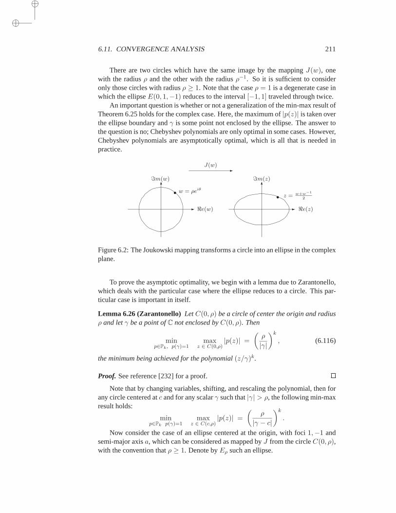
6.11. CONVERGENCE ANALYSIS 211
There are two circles which have the same image by the mappingJ(w), onewith the radiusρ and the other with the radiusρ−1. So it is sufficient to consideronly those circles with radiusρ ≥ 1. Note that the caseρ = 1 is a degenerate case inwhich the ellipseE(0, 1,−1) reduces to the interval[−1, 1] traveled through twice.
An important question is whether or not a generalization of the min-max result ofTheorem 6.25 holds for the complex case. Here, the maximum of|p(z)| is taken overthe ellipse boundary andγ is some point not enclosed by the ellipse. The answer tothe question is no; Chebyshev polynomials are only optimal in some cases. However,Chebyshev polynomials are asymptotically optimal, which is all that is needed inpractice.
-
6
ℜe(w)
ℑm(w)
w = ρeiθ•
-J(w)
-
6
ℜe(z)
ℑm(z)
z = w+w−1
2•
Figure 6.2: The Joukowski mapping transforms a circle into an ellipse in the complexplane.
To prove the asymptotic optimality, we begin with a lemma due to Zarantonello,which deals with the particular case where the ellipse reduces to a circle. Thispar-ticular case is important in itself.
Lemma 6.26 (Zarantonello) LetC(0, ρ) be a circle of center the origin and radiusρ and letγ be a point ofC not enclosed byC(0, ρ). Then
minp∈Pk, p(γ)=1
maxz ∈ C(0,ρ)
|p(z)| =
(ρ
|γ|
)k
, (6.116)
the minimum being achieved for the polynomial(z/γ)k.
Proof. See reference [232] for a proof.
Note that by changing variables, shifting, and rescaling the polynomial, thenforany circle centered atc and for any scalarγ such that|γ| > ρ, the following min-maxresult holds:
minp∈Pk p(γ)=1
maxz ∈ C(c,ρ)
|p(z)| =
(ρ
|γ − c|
)k
.
Now consider the case of an ellipse centered at the origin, with foci1,−1 andsemi-major axisa, which can be considered as mapped byJ from the circleC(0, ρ),with the convention thatρ ≥ 1. Denote byEρ such an ellipse.
212 CHAPTER 6. KRYLOV SUBSPACE METHODS PART I
Theorem 6.27 Consider the ellipseEρ mapped fromC(0, ρ) by the mappingJ andlet γ be any point in the complex plane not enclosed by it. Then
ρk
|wγ |k≤ min
p∈Pk p(γ)=1max
z ∈ Eρ
|p(z)| ≤ ρk + ρ−k
|wkγ + w−k
γ |(6.117)
in whichwγ is the dominant root of the equationJ(w) = γ.
Proof. We start by showing the second inequality. Any polynomialp of degreeksatisfying the constraintp(γ) = 1 can be written as
p(z) =
∑kj=0 ξjz
j
∑kj=0 ξjγ
j.
A point z on the ellipse is transformed byJ from a certainw in C(0, ρ). Similarly,let wγ be one of the two inverse transforms ofγ by the mapping, namely, the onewith largest modulus. Then,p can be rewritten as
p(z) =
∑kj=0 ξj(w
j + w−j)∑k
j=0 ξj(wjγ + w−j
γ ). (6.118)
Consider the particular polynomial obtained by settingξk = 1 andξj = 0 for j 6= k,
p∗(z) =wk + w−k
wkγ + w−k
γ
which is a scaled Chebyshev polynomial of the first kind of degreek in the variablez.It is apparent that the maximum modulus of this polynomial is reached in particularwhenw = ρeiθ is real, i.e., whenw = ρ. Thus,
maxz∈Eρ
|p∗(z)| = ρk + ρ−k
|wkγ + w−k
γ |
which proves the second inequality.To prove the left inequality, we rewrite (6.118) as
p(z) =
(
w−k
w−kγ
) ∑kj=0 ξj(w
k+j + wk−j)∑k
j=0 ξj(wk+jγ + wk−j
γ )
and take the modulus ofp(z),
|p(z)| = ρ−k
|wγ |−k
∣∣∣∣∣
∑kj=0 ξj(w
k+j + wk−j)∑k
j=0 ξj(wk+jγ + wk−j
γ )
∣∣∣∣∣.
The polynomial inw of degree2k inside the large modulus bars in the right-hand sideis such that its value atwγ is one. By Lemma 6.26, the modulus of this polynomial
6.11. CONVERGENCE ANALYSIS 213
over the circleC(0, ρ) is not less than(ρ/|wγ |)2k, i.e., for any polynomial, satisfyingthe constraintp(γ) = 1,
maxz∈ Eρ
|p(z)| ≥ ρ−k
|wγ |−k
ρ2k
|wγ |2k=
ρk
|wγ |k.
This proves that the minimum over all such polynomials of the maximum moduluson the ellipseEρ is≥ (ρ/|wγ |)k.
The difference between the left and right bounds in (6.117) tends to zero askincreases to infinity. Thus, the important point made by the theorem is that forlargek, the Chebyshev polynomial
p∗(z) =wk + w−k
wkγ + w−k
γ
, where z =w + w−1
2
is close to the optimal polynomial. More specifically, Chebyshev polynomials areasymptoticallyoptimal.
For a more general ellipseE(c, d, a) centered atc, and with focal distanced andsemi-major axisa, a simple change of variables shows that the near-best polynomialis given by
Ck(z) =Ck
(c−zd
)
Ck
( c−γd
) . (6.119)
In addition, by examining the expression(wk + w−k)/2 for w = ρeiθ it is easilyseen that the maximum modulus ofCk(z), i.e., the infinity norm of this polynomialover the ellipse, is reached at the pointc + a located on the real axis. From this weget,
maxz ∈ E(c,d,a)
|Ck(z)| =Ck
(ad
)
|Ck
( c−γd
)|
Here, we point out thatd anda both can be purely imaginary [for an example, see part(B) of Figure 6.3]. In this casea/d is real and the numerator in the above expressionis always real. Using the definition forCk we obtain the following useful expressionand approximation:
Ck
(ad
)
Ck
( c−γd
) =
(
ad +
√(
ad
)2 − 1
)k
+
(
ad +
√(
ad
)2 − 1
)−k
(
c−γd +
√( c−γ
d
)2 − 1
)k
+
(
c−γd +
√( c−γ
d
)2 − 1
)−k(6.120)
≈(
a+√a2 − d2
c− γ +√
(c− γ)2 − d2
)k
(6.121)
Finally, we note that an alternative and more detailed result has been proven byFischer and Freund in [127].

214 CHAPTER 6. KRYLOV SUBSPACE METHODS PART I
6.11.3 Convergence of the CG Algorithm
As usual,‖x‖A denotes the norm defined by
‖x‖A = (Ax, x)1/2.
The following lemma characterizes the approximation obtained from the ConjugateGradient algorithm.
Lemma 6.28 Letxm be the approximate solution obtained from them-th step of theCG algorithm, and letdm = x∗ − xm wherex∗ is the exact solution. Then,xm is ofthe form
xm = x0 + qm(A)r0
whereqm is a polynomial of degreem− 1 such that
‖(I −Aqm(A))d0‖A = minq ∈ Pm−1
‖(I −Aq(A))d0‖A.
Proof. This is a consequence of the fact thatxm minimizes theA-norm of the errorin the affine subspacex0 + Km, a result of Proposition 5.2, and the fact thatKm isthe set of all vectors of the formx0 + q(A)r0, whereq is a polynomial of degree≤ m− 1.
From this, the following theorem can be proved.
Theorem 6.29 Letxm be the approximate solution obtained at them-th step of theConjugate Gradient algorithm, andx∗ the exact solution and define
η =λmin
λmax − λmin. (6.122)
Then,
‖x∗ − xm‖A ≤‖x∗ − x0‖ACm(1 + 2η)
, (6.123)
in whichCm is the Chebyshev polynomial of degreem of the first kind.
Proof. From the previous lemma, it is known that‖x∗ − xm‖A minimizesA-normof the error over polynomialsr(t) which take the value one at0, i.e.,
‖x∗ − xm‖A = minr∈ Pm, r(0)=1
‖r(A)d0‖A.
If λi, i = 1, . . . , n are the eigenvalues ofA, andξi, i = 1, . . . , n the components ofthe initial errord0 in the eigenbasis, then
‖r(A)d0‖2A =n∑
i=1
λir(λi)2(ξi)
2 ≤ maxi
(r(λi))2‖d0‖2A
≤ maxλ ∈[λmin,λmax]
(r(λ))2‖d0‖2A.
6.11. CONVERGENCE ANALYSIS 215
Therefore,
‖x∗ − xm‖A ≤ minr∈ Pm, r(0)=1
maxλ ∈[λmin,λmax]
|r(λ)|‖d0‖A.
The result follows immediately by using the well known result of Theorem 6.25fromapproximation theory. This gives the polynomialr which minimizes the right-handside.
A slightly different formulation of inequality (6.123) can be derived. Usingtherelation,
Cm(t) =1
2
[(
t+√
t2 − 1)m
+(
t+√
t2 − 1)−m
]
≥ 1
2
(
t+√
t2 − 1)m
then
Cm(1 + 2η) ≥ 1
2
(
1 + 2η +√
(1 + 2η)2 − 1)m
≥ 1
2
(
1 + 2η + 2√
η(η + 1))m
.
Now notice that
1 + 2η + 2√
η(η + 1) =(√
η +√
η + 1)2
(6.124)
=
(√λmin +
√λmax
)2
λmax − λmin(6.125)
=
√λmax +
√λmin√
λmax −√λmin
(6.126)
=
√κ+ 1√κ− 1
(6.127)
in whichκ is the spectral condition numberκ = λmax/λmin.Substituting this in (6.123) yields,
‖x∗ − xm‖A ≤ 2
[√κ− 1√κ+ 1
]m
‖x∗ − x0‖A. (6.128)
This bound is similar to that of the steepest descent algorithm except that thecondi-tion number ofA is now replaced by its square root.
6.11.4 Convergence of GMRES
We begin by stating aglobal convergence result. Recall that a matrixA is calledpositive definite if its symmetric part(A + AT )/2 is Symmetric Positive Definite.This is equivalent to the property that(Ax, x) > 0 for all nonzero real vectorsx.
216 CHAPTER 6. KRYLOV SUBSPACE METHODS PART I
Theorem 6.30 If A is a positive definite matrix, then GMRES(m) converges for anym ≥ 1.
Proof. This is true because the subspaceKm contains the initial residual vector ateach restart. Since the algorithm minimizes the residual norm in the subspaceKm,at each outer iteration, the residual norm will be reduced by as much as theresult ofone step of the Minimal Residual method seen in the previous chapter. Therefore, theinequality (5.15) is satisfied by residual vectors produced after each outer iterationand the method converges.
Next we wish to establish a result similar to the one for the Conjugate Gradientmethod, which would provide an upper bound on the convergence rate ofthe GMRESiterates. We begin with a lemma similar to Lemma 6.28.
Lemma 6.31 Letxm be the approximate solution obtained from them-th step of theGMRES algorithm, and letrm = b−Axm. Then,xm is of the form
xm = x0 + qm(A)r0
and‖rm‖2 = ‖(I −Aqm(A))r0‖2 = min
q ∈ Pm−1
‖(I −Aq(A))r0‖2.
Proof. This is true becausexm minimizes the2-norm of the residual in the affinesubspacex0 + Km, a result of Proposition 5.3, and the fact thatKm is the set of allvectors of the formx0 + q(A)r0, whereq is a polynomial of degree≤ m− 1.
Unfortunately, it not possible to prove a simple result such as Theorem 6.29 unlessA is normal.
Proposition 6.32 Assume thatA is a diagonalizable matrix and letA = XΛX−1
whereΛ = diag λ1, λ2, . . . , λn is the diagonal matrix of eigenvalues. Define,
ǫ(m) = minp∈Pm,p(0)=1
maxi=1,...,n
|p(λi)|.
Then, the residual norm achieved by them-th step of GMRES satisfies the inequality
‖rm‖2 ≤ κ2(X)ǫ(m)‖r0‖2.
whereκ2(X) ≡ ‖X‖2‖X−1‖2.
Proof. Let p be any polynomial of degree≤ m which satisfies the constraintp(0) =1, andx the vector inKm to which it is associated viab−Ax = p(A)r0. Then,
‖b−Ax‖2 = ‖Xp(Λ)X−1r0‖2 ≤ ‖X‖2‖X−1‖2‖r0‖2‖p(Λ)‖2

6.11. CONVERGENCE ANALYSIS 217
SinceΛ is diagonal, observe that
‖p(Λ)‖2 = maxi=1,...,n
|p(λi)|.
Sincexm minimizes the residual norm overx0 + Km, then for any consistent poly-nomialp,
‖b−Axm‖ ≤ ‖b−Ax‖2 ≤ ‖X‖2‖X−1‖2‖r0‖2 maxi=1,...,n
|p(λi)|.
Now the polynomialp which minimizes the right-hand side in the above inequalitycan be used. This yields the desired result,
‖b−Axm‖ ≤ ‖b−Ax‖2 ≤ ‖X‖2‖X−1‖2‖r0‖2ǫ(m).
-
6
ℜe(z)
ℑm(z)
c c + dc − d c + a
c − aI
(A)
-
6
ℜe(z)
ℑm(z)
c
c + d
c − d
c + a
c − a
(B)
Figure 6.3: Ellipses containing the spectrum ofA. Case (A): reald; case (B): purelyimaginaryd.
The results of Section 6.11.2 on near-optimal Chebyshev polynomials in thecomplex plane can now be used to obtain an upper bound forǫ(m). Assume thatthe spectrum ofA in contained in an ellipseE(c, d, a) with centerc, focal distanced, and major semi axisa. In addition it is required that the origin lie outside thisellipse. The two possible cases are shown in Figure 6.3. Case (B) corresponds tothe situation whend is purely imaginary, i.e., the major semi-axis is aligned with theimaginary axis.
Corollary 6.33 LetA be a diagonalizable matrix, i.e, letA = XΛX−1 whereΛ =diag λ1, λ2, . . . , λn is the diagonal matrix of eigenvalues. Assume that all the
218 CHAPTER 6. KRYLOV SUBSPACE METHODS PART I
eigenvalues ofA are located in the ellipseE(c, d, a) which excludes the origin. Then,the residual norm achieved at them-th step of GMRES satisfies the inequality,
‖rm‖2 ≤ κ2(X)Cm
(ad
)
∣∣Cm
(cd
)∣∣‖r0‖2.
Proof. All that is needed is an upper bound for the scalarǫ(m) under the assumptions.By definition,
ǫ(m) = minp∈Pm,p(0)=1
maxi=1,...,n
|p(λi)|
≤ minp∈Pm,p(0)=1
maxλ ∈ E(c,d,a)
|p(λ)|.
The second inequality is due to the fact that the maximum modulus of a complexanalytical function is reached on the boundary of the domain. We can now use as atrial polynomialCm defined by (6.119), withγ = 0:
ǫ(m) ≤ minp∈Pm,p(0)=1
maxλ ∈ E(c,d,a)
|p(λ)|
≤ maxλ ∈ E(c,d,a)
|Cm(λ)| = Cm
(ad
)
∣∣Cm
(cd
)∣∣.
This completes the proof.
An explicit expression for the coefficientCm
(ad
)/ Cm
(cd
)and an approximation
are readily obtained from (6.120-6.121) by takingγ = 0:
Cm
(ad
)
Cm
(cd
) =
(
ad +
√(
ad
)2 − 1
)m
+
(
ad +
√(
ad
)2 − 1
)−m
(
cd +
√(
cd
)2 − 1
)m
+
(
cd +
√(
cd
)2 − 1
)−m
≈(
a+√a2 − d2
c+√c2 − d2
)m
.
Since the condition numberκ2(X) of the matrix of eigenvectorsX is typicallynot known and can be very large, results of the nature of the corollary are of limitedpractical interest. They can be useful only when it is known that the matrix isnearlynormal, in which case,κ2(X) ≈ 1.
6.12 Block Krylov Methods
In many circumstances, it is desirable to work with a block of vectors instead ofa single vector. For example, out-of-core finite-element codes are more efficientwhen they are programmed to exploit the presence of a block of the matrixA in fastmemory, as much as possible. This can be achieved by using block generalizations of
6.12. BLOCK KRYLOV METHODS 219
Krylov subspace methods, for whichA always operates on a group of vectors insteadof a single vector. We begin by describing a block version of the Arnoldi algorithm.
ALGORITHM 6.22 Block Arnoldi
1. Choose a unitary matrixV1 of dimensionn× p.2. Forj = 1, 2, . . . ,m Do:3. ComputeHij = V T
i AVj i = 1, 2, . . . , j
4. ComputeWj = AVj −∑j
i=1 ViHij
5. Compute the Q-R factorization ofWj : Wj = Vj+1Hj+1,j
6. EndDo
The above algorithm is a straightforward block analogue of Algorithm 6.1. Byconstruction, the blocks generated by the algorithm are orthogonal blocks that arealso orthogonal to each other. In the following we denote byIk thek × k identitymatrix and use the following notation:
Um = [V1, V2, . . . , Vm],
Hm = (Hij)1≤i,j≤m, Hij ≡ 0, for i > j + 1,
Em = matrix of the lastp columns ofImp.
Then, the following analogue of the relation (6.6) is easily proved:
AUm = UmHm + Vm+1Hm+1,mETm. (6.129)
Here, the matrixHm is no longer Hessenberg, but band-Hessenberg, meaning that ithasp subdiagonals instead of only one. Note that the dimension of the subspace inwhich the solution is sought is notm butm.p.
A second version of the algorithm uses a modified block Gram-Schmidt proce-dure instead of the simple Gram-Schmidt procedure used above. This leadsto a blockgeneralization of Algorithm 6.2, the Modified Gram-Schmidt version of Arnoldi’smethod.
ALGORITHM 6.23 Block Arnoldi with Block MGS
1. Choose a unitary matrixV1 of sizen× p2. Forj = 1, 2, . . . ,m Do:3. ComputeWj := AVj
4. Fori = 1, 2, . . . , j do:5. Hij := V T
i Wj
6. Wj := Wj − ViHij
7. EndDo8. Compute the Q-R decompositionWj = Vj+1Hj+1,j
9. EndDo
Again, in practice the above algorithm is more viable than its predecessor. Fi-nally, a third version, developed by A. Ruhe [236] for the symmetric case (block
220 CHAPTER 6. KRYLOV SUBSPACE METHODS PART I
Lanczos), yields a variant that is quite similar to the original Arnoldi algorithm.As-sume that the initial block ofp orthonormal vectors,v1, . . . , vp is available. The firststep of the algorithm is to multiplyv1 byA and orthonormalize the resulting vectorw againstv1, . . . , vp. The resulting vector is defined to bevp+1. In the second stepit is v2 that is multiplied byA and orthonormalized against all availablevi’s. Thus,the algorithm works similarly to Algorithm 6.2 except for a delay in the vector thatis multiplied byA at each step.
ALGORITHM 6.24 Block Arnoldi–Ruhe’s variant
1. Choosep initial orthonormal vectorsvii=1,...,p.2. Forj = p, p+ 1, . . . ,m+ p− 1 Do:3. Setk := j − p+ 1;4. Computew := Avk;5. Fori = 1, 2, . . . , j Do:6. hi,k := (w, vi)7. w := w − hi,kvi
8. EndDo9. Computehj+1,k := ‖w‖2 andvj+1 := w/hj+1,k.
10. EndDo
Observe that the particular casep = 1 coincides with the usual Arnoldi process.Also, the dimensionm of the subspace of approximants, is no longer restricted tobeing a multiple of the block-sizep as in the previous algorithms. The mathematicalequivalence of Algorithms 6.23 and 6.24 whenm is a multiple ofp is straightfor-ward to show. The advantage of the above formulation is its simplicity. A slightdisadvantage is that it gives up some potential parallelism. In the original version,the columns of the matrixAVj can be computed in parallel whereas in the new algo-rithm, they are computed in sequence. This can be remedied, however, by performingp matrix-by-vector products everyp steps.
At the end of the loop consisting of lines 5 through 8 of Algorithm 6.24, thevectorw satisfies the relation
w = Avk −j∑
i=1
hikvi,
wherek andj are related byk = j − p + 1. Line 9 givesw = hj+1,kvj+1 whichresults in
Avk =
k+p∑
i=1
hikvi.
As a consequence, the analogue of the relation (6.7) for Algorithm 6.24 is
AVm = Vm+pHm. (6.130)
As before, for anyj the matrixVj represents then×j matrix with columnsv1, . . . vj .The matrixHm is now of size(m+ p)×m.
6.12. BLOCK KRYLOV METHODS 221
Now the block generalizations of FOM and GMRES can be defined in a straight-forward way. These block algorithms can solve linear systems with multiple right-hand sides,
Ax(i) = b(i), i = 1, · · · , p, (6.131)
or, in matrix formAX = B, (6.132)
where the columns of then × p matricesB andX are theb(i)’s andx(i)’s, respec-tively. Given an initial block of initial guessesx(i)
0 for i = 1, . . . , p, we defineR0 theblock of initial residuals
R0 ≡ [r(1)0 , r
(2)0 , . . . , r
(p)0 ],
where each column isr(i)0 = b(i) − Ax(i)0 . It is preferable to use the unified notation
derived from Algorithm 6.24. In this notation,m is not restricted to being a multipleof the block-sizep and the same notation is used for thevi’s as in the scalar ArnoldiAlgorithm. Thus, the first step of the block-FOM or block-GMRES algorithm istocompute the QR factorization of the block of initial residuals:
R0 = [v1, v2, . . . , vp] R.
Here, the matrix[v1, . . . , vp] is unitary andR is p × p upper triangular. This factor-ization provides the firstp vectors of the block-Arnoldi basis.
Each of the approximate solutions has the form
x(i) = x(i)0 + Vmy
(i), (6.133)
and, grouping these approximationsx(i) in a blockX and they(i) in a blockY , wecan write
X = X0 + VmY. (6.134)
It is now possible to imitate what was done for the standard FOM and GMRESalgorithms. The only missing link is the vectorβe1 in (6.27) which now becomes amatrix. LetE1 be the(m + p) × p matrix whose upperp × p principal block is anidentity matrix. Then, the relation (6.130) results in
B −AX = B −A (X0 + VmY )
= R0 −AVmY
= [v1, . . . , vp]R− Vm+pHmY
= Vm+p
(E1R− HmY
). (6.135)
The vectorg(i) ≡ E1Rei
is a vector of lengthm+pwhose components are zero except those from 1 toiwhichare extracted from thei-th column of the upper triangular matrixR. The matrixHm
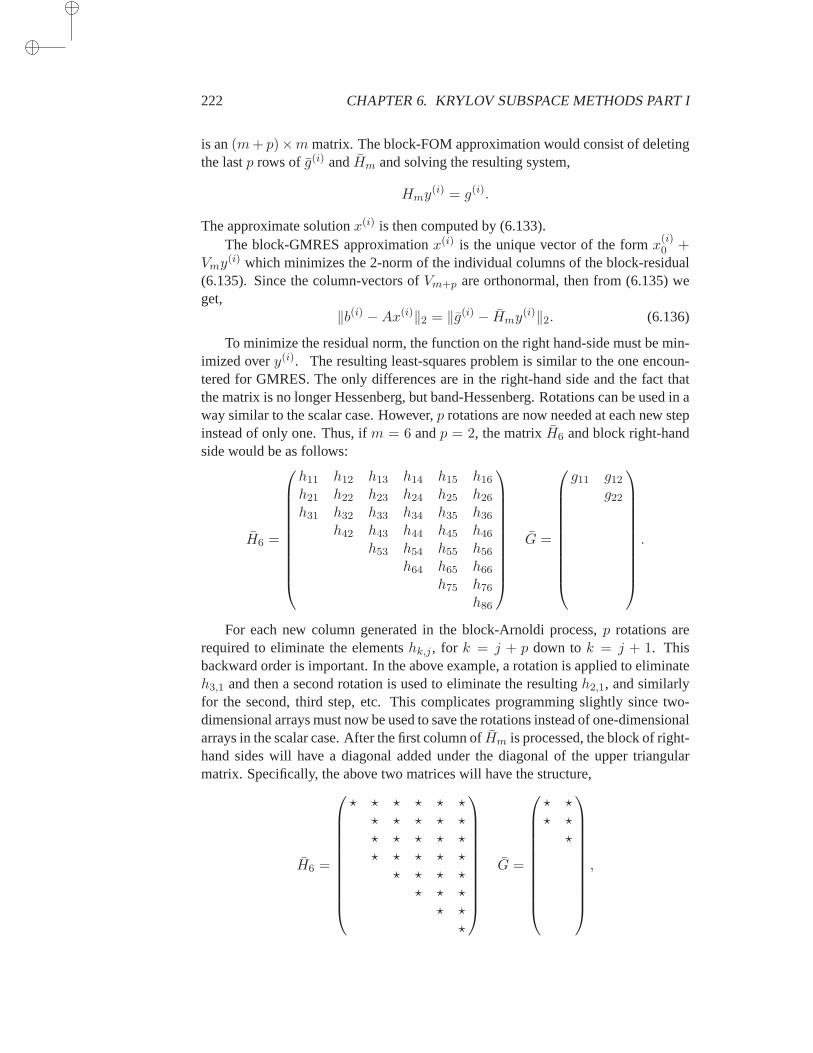
222 CHAPTER 6. KRYLOV SUBSPACE METHODS PART I
is an(m+ p)×m matrix. The block-FOM approximation would consist of deletingthe lastp rows of g(i) andHm and solving the resulting system,
Hmy(i) = g(i).
The approximate solutionx(i) is then computed by (6.133).The block-GMRES approximationx(i) is the unique vector of the formx(i)
0 +Vmy
(i) which minimizes the 2-norm of the individual columns of the block-residual(6.135). Since the column-vectors ofVm+p are orthonormal, then from (6.135) weget,
‖b(i) −Ax(i)‖2 = ‖g(i) − Hmy(i)‖2. (6.136)
To minimize the residual norm, the function on the right hand-side must be min-imized overy(i). The resulting least-squares problem is similar to the one encoun-tered for GMRES. The only differences are in the right-hand side and thefact thatthe matrix is no longer Hessenberg, but band-Hessenberg. Rotations can be used in away similar to the scalar case. However,p rotations are now needed at each new stepinstead of only one. Thus, ifm = 6 andp = 2, the matrixH6 and block right-handside would be as follows:
H6 =
h11 h12 h13 h14 h15 h16
h21 h22 h23 h24 h25 h26
h31 h32 h33 h34 h35 h36
h42 h43 h44 h45 h46
h53 h54 h55 h56
h64 h65 h66
h75 h76
h86
G =
g11 g12g22
.
For each new column generated in the block-Arnoldi process,p rotations arerequired to eliminate the elementshk,j , for k = j + p down tok = j + 1. Thisbackward order is important. In the above example, a rotation is applied to eliminateh3,1 and then a second rotation is used to eliminate the resultingh2,1, and similarlyfor the second, third step, etc. This complicates programming slightly since two-dimensional arrays must now be used to save the rotations instead of one-dimensionalarrays in the scalar case. After the first column ofHm is processed, the block of right-hand sides will have a diagonal added under the diagonal of the upper triangularmatrix. Specifically, the above two matrices will have the structure,
H6 =
⋆ ⋆ ⋆ ⋆ ⋆ ⋆⋆ ⋆ ⋆ ⋆ ⋆⋆ ⋆ ⋆ ⋆ ⋆⋆ ⋆ ⋆ ⋆ ⋆
⋆ ⋆ ⋆ ⋆⋆ ⋆ ⋆
⋆ ⋆⋆
G =
⋆ ⋆⋆ ⋆
⋆
,
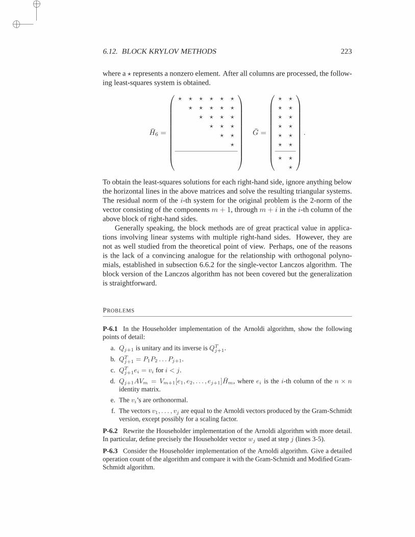
6.12. BLOCK KRYLOV METHODS 223
where a⋆ represents a nonzero element. After all columns are processed, the follow-ing least-squares system is obtained.
H6 =
⋆ ⋆ ⋆ ⋆ ⋆ ⋆⋆ ⋆ ⋆ ⋆ ⋆
⋆ ⋆ ⋆ ⋆⋆ ⋆ ⋆
⋆ ⋆⋆
G =
⋆ ⋆⋆ ⋆⋆ ⋆⋆ ⋆⋆ ⋆⋆ ⋆
⋆ ⋆⋆
.
To obtain the least-squares solutions for each right-hand side, ignore anything belowthe horizontal lines in the above matrices and solve the resulting triangular systems.The residual norm of thei-th system for the original problem is the 2-norm of thevector consisting of the componentsm+ 1, throughm+ i in thei-th column of theabove block of right-hand sides.
Generally speaking, the block methods are of great practical value in applica-tions involving linear systems with multiple right-hand sides. However, they arenot as well studied from the theoretical point of view. Perhaps, one of the reasonsis the lack of a convincing analogue for the relationship with orthogonal polyno-mials, established in subsection 6.6.2 for the single-vector Lanczos algorithm.Theblock version of the Lanczos algorithm has not been covered but the generalizationis straightforward.
PROBLEMS
P-6.1 In the Householder implementation of the Arnoldi algorithm, show the followingpoints of detail:
a. Qj+1 is unitary and its inverse isQTj+1.
b. QTj+1 = P1P2 . . . Pj+1.
c. QTj+1ei = vi for i < j.
d. Qj+1AVm = Vm+1[e1, e2, . . . , ej+1]Hm, whereei is the i-th column of then × nidentity matrix.
e. Thevi’s are orthonormal.
f. The vectorsv1, . . . , vj are equal to the Arnoldi vectors produced by the Gram-Schmidtversion, except possibly for a scaling factor.
P-6.2 Rewrite the Householder implementation of the Arnoldi algorithm with more detail.In particular, define precisely the Householder vectorwj used at stepj (lines 3-5).
P-6.3 Consider the Householder implementation of the Arnoldi algorithm. Give a detailedoperation count of the algorithm and compare it with the Gram-Schmidt and Modified Gram-Schmidt algorithm.
224 CHAPTER 6. KRYLOV SUBSPACE METHODS PART I
P-6.4 Consider a variant of the GMRES algorithm in which the Arnoldi process starts withv1 = Av0/‖Av0‖2 wherev0 ≡ r0. The Arnoldi process is performed the same way asbefore to build an orthonormal systemv1, v2, . . . , vm−1. Now the approximate solution isexpressed in the basisv0, v1, . . . , vm−1.
a. Show that the least squares problem that must be solved to obtain the approximatesolution is now triangular instead of Hessemberg.
b. Show that the residual vectorrk is orthogonal tov1, v2, . . . , vk−1.
c. Find a formula which computes the residual norm (without computing the approximatesolution) and write the complete algorithm.
P-6.5 Derive the basic version of GMRES by using the standard formula (5.7) withV = Vm
andW = AVm.
P-6.6 Analyze the arithmic cost, i.e., the number of operations, of Algorithms 6.7 and 6.8.Similarly analyse the memory requirement of both algorithms.
P-6.7 Derive a version of the DIOM algorithm which includes partial pivoting in the solu-tion of the Hessenberg system.
P-6.8 Show how the GMRES and FOM methods will converge on the linearsystemAx = bwhen
A =
11
11
1
, b =
10000
and withx0 = 0.
P-6.9 Give a full proof of Proposition 6.17.
P-6.10 Let a matrixA have the form
A =
(I Y0 I
)
.
Assume that (full) GMRES is used to solve a linear system, with the coefficient matrixA.What is the maximum number of steps that GMRES would require toconverge?
P-6.11 Let a matrixA have the form:
A =
(I Y0 S
)
.
Assume that (full) GMRES is used to solve a linear system withthe coefficient matrixA. Let
r0 =
(r(1)0
r(2)0
)
be the initial residual vector. It is assumed that the degreeof the minimal polynomial ofr(2)0
with respect toS (i.e., its grade) isk. What is the maximum number of steps that GMRESwould require to converge for this matrix? [Hint: Evaluate the sum
∑ki=0 βi(A
i+1 − Ai)r0where
∑ki=0 βit
i is the minimal polynomial ofr(2)0 with respect toS.]
6.12. BLOCK KRYLOV METHODS 225
P-6.12 Let
A =
I Y2
I Y3
I.. .I Yk−1
I Yk
I
.
a. Show that(I −A)k = 0.
b. Assume that (full) GMRES is used to solve a linear system with the coefficient matrixA. What is the maximum number of steps that GMRES would require to converge?
P-6.13 Show that ifHm is nonsingular, i.e., when the FOM iteratexFm is defined, and if the
GMRES iteratexGm is such thatxG
m = xFm, thenrG
m = rFm = 0, i.e., both the GMRES and
FOM solutions are exact. [Hint: use the relation (6.74) and Proposition 6.17 or Proposition6.12.]
P-6.14 Derive the relation (6.63) from (6.75). [Hint: Use the fact that the vectors on theright-hand side of (6.75) are orthogonal.]
P-6.15 In the Householder-GMRES algorithm the approximate solution can be computedby formulas (6.31-6.33). What is the exact cost of this alternative (compare memory as wellas arithmetic requirements)? How does it compare with the cost of keeping thevi’s?
P-6.16 An alternative to formulas (6.31-6.33) for accumulating the approximate solution inthe Householder-GMRES algorithm without keeping thevi’s is to computexm as
xm = x0 + P1P2 . . . Pmy
wherey is a certainn-dimensional vector to be determined. (1) What is the vectory forthe above formula in order to compute the correct approximate solutionxm? [Hint: Exploit(6.13).] (2) Write down an alternative to formulas (6.31-6.33) derived from this approach.(3) Compare the cost of this approach with the cost of using (6.31-6.33).
P-6.17 Obtain the formula (6.97) from (6.96).
P-6.18 Show that the determinant of the matrixTm in (6.103) is given by
det (Tm) =1
∏m−1i=0 αi
.
P-6.19 The Lanczos algorithm is more closely related to the implementation of Algorithm6.19 of the Conjugate Gradient algorithm. As a result the Lanczos coefficientsδj+1 andηj+1
are easier to extract from this algorithm than from Algorithm 6.18. Obtain formulas for thesecoefficients from the coefficients generated by Algorithm 6.19, as was done in Section 6.7.3for the standard CG algorithm.
P-6.20 What can be said of the Hessenberg matrixHm whenA is skew-symmetric? Whatdoes this imply on the Arnoldi algorithm?
P-6.21 Consider a matrix of the form
A = I + αB (6.137)
whereB is skew-symmetric (real), i.e., such thatBT = −B.
a. Show that(Ax, x)/(x, x) = 1 for all nonzerox.
226 CHAPTER 6. KRYLOV SUBSPACE METHODS PART I
b. Consider the Arnoldi process forA. Show that the resulting Hessenberg matrix willhave the following tridiagonal form
Hm =
1 −η2η2 1 −η3
. . .ηm−1 1 −ηm
ηm 1
.
c. Using the result of the previous question, explain why theCG algorithm applied as isto a linear system with the matrixA, which is nonsymmetric, will still yield residualvectors that are orthogonal to each other.
P-6.22 Establish the three relations (6.22), (6.23), and (6.24).
P-6.23 Show that if the rotations generated in the course of the GMRES (and DQGMRES)algorithm are such that
|cm| ≥ c > 0,
then GMRES, DQGMRES, and FOM will all converge.
P-6.24 Show the exact expression of the residual vector in the basisv1, v2, . . . , vm+1 foreither GMRES or DQGMRES. [Hint: A starting point is (6.50).]
P-6.25 Prove that the inequality (6.54) is sharper than (6.51), in the sense thatζm+1 ≤√m− k + 1 (for m ≥ k). [Hint: Use Cauchy-Schwarz inequality on (6.54).]
P-6.26 Consider the minimal residual smoothing algorithm (Algorithm 7.5) in the situationwhen the residual vectorsrO
j of the original sequence are orthogonal to each other. Showthat the vectors
rOj − rS
j−1 = −A(xOj − xS
j−1)
are orthogonal to each other [Hint: use induction]. Then useLemma 6.21 to conclude thatthe iterates of the algorithm are identical with those of ORTHOMIN and GMRES.
P-6.27 Consider the complex GMRES algorithm in Section 6.5.9. Showat least two otherways of defining complex Givens rotations (the requirement is thatΩi be a unitary matrix,i.e., thatΩH
i Ωi = I). Which among the three possible choices give (s) a nonnegative realdiagonal for the resultingRm matrix?
P-6.28 Work out the details of a Householder implementation of the GMRES algorithm forcomplex linear systems (The Householder matrices are now ofthe formI−2wwH ; part of thepractical implementation details is already available forthe complex case in Section 6.5.9.)
P-6.29 Denote bySm the unit upper triangular matrixS in the proof of Theorem 6.11which is obtained from the Gram-Schmidt process (exact arithmetic assumed) applied to theincomplete orthogonalization basisVm. Show that the Hessenberg matrixHQ
m obtained inthe incomplete orthogonalization process is related to theHessenberg matrixHG
m obtainedfrom the (complete) Arnoldi process by
HGm = S−1
m+1HQmSm.
NOTES AND REFERENCES. The Conjugate Gradient method was developed independently and indifferent forms by Lanczos [197] and Hestenes and Stiefel [167].The method was essentially viewedas a direct solution technique and was abandoned early on because it didnot compare well with otherexisting techniques. For example, in inexact arithmetic, the method does not terminate inn steps as
6.12. BLOCK KRYLOV METHODS 227
is predicted by the theory. This is caused by the severe loss of of orthogonality of vector quantitiesgenerated by the algorithm. As a result, research on Krylov-type methods remained dormant for overtwo decades thereafter. This changed in the early 1970s when severalresearchers discovered that thisloss of orthogonality did not prevent convergence. The observationswere made and explained foreigenvalue problems [222, 147] as well as linear systems [231]. The early to the middle 1980s sawthe development of a new class of methods for solving nonsymmetric linear systems [12, 13, 178, 238,239, 251, 298]. The works of Faber and Manteuffel [121] and Voevodin [299] showed that one couldnot find optimal methods which, like CG, are based on short-term recurrences. Many of the methodsdeveloped are mathematically equivalent, in the sense that they realize the same projection process,with different implementations.
Lemma 6.16 was proved by Roland Freund [134] in a slightly different form. Proposition 6.12 isdue to Brown [66] who proved a number of other theoretical results, including Proposition 6.17. Theinequality (6.64), which can be viewed as a reformulation of Brown’s result, was proved by Cullumand Greenbaum [92]. This result is equivalent to Equation (6.67) which was shown in a very differentway by Zhou and Walker [324].
The Householder version of GMRES is due to Walker [303]. The Quasi-GMRES algorithm de-scribed in Section 6.5.6 was initially described by Brown and Hindmarsh [67], and the direct versionDQGMRES was discussed in [255]. The proof of Theorem 6.11 for DQGMRES is adapted from theresult shown in [213] for the QMR algorithm.
Schonauer [260] seems to have been the originator or Minimal Residual Smoothing methods,but Weiss [307] established much of the theory and connections with othertechniques. The Quasi-minimization extension of these techniques (QMRS) was developed by Zhouand Walker [324].
The non-optimality of the Chebyshev polynomials on ellipses in the complex plane was estab-lished by Fischer and Freund [128]. Prior to this, a 1963 paper by Clayton [86] was believed to haveestablished the optimality for the special case where the ellipse has real foci andγ is real.
Various types of Block Krylov methods were considered. In addition to their attraction for solvinglinear systems with several right-hand sides [243, 267], one of the other motivations for these techniquesis that they can also help reduce the effect of the sequential inner products in parallel environmentsand minimize I/O costs in out-of-core implementations. A block Lanczos algorithm was developedby Underwood [287] for the symmetric eigenvalue problem, while O’Leary discussed a block CGalgorithm [215]. The block-GMRES algorithm is analyzed by Simoncini andGallopoulos [266] and in[250]. Besides the straightforward extension presented in Section 6.12, a variation was developed byJbilou et al., in which a ‘global’ inner product for the blocks was considered instead of the usual scalarinner product for each column [176].
Alternatives to GMRES which require fewer inner products have been proposed by Sadok [256]and Jbilou [175]. Sadok investigated a GMRES-like method based on the Hessenberg algorithm [317],while Jbilou proposed a multi-dimensional generalization of Gastinel’s method seen in Exercise 2 ofChapter 5.

228 CHAPTER 6. KRYLOV SUBSPACE METHODS PART I
Chapter 7
KRYLOV SUBSPACE METHODS PART II
The previous chapter considered a number of Krylov subspace methods which relied on some
form of orthogonalization of the Krylov vectors in order to compute an approximate solution.
This chapter will describe a class of Krylov subspace methods which are instead based on a bi-
orthogonalization algorithm due to Lanczos. These are projection methods that are intrinsically
non-orthogonal. They have some appealing properties, but are harder to analyze theoretically.
7.1 Lanczos Biorthogonalization
The Lanczos biorthogonalization algorithm is an extension to nonsymmetric matri-ces of the symmetric Lanczos algorithm seen in the previous chapter. One suchextension, the Arnoldi procedure, has already been seen. However, the nonsymmet-ric Lanczos algorithm is quite different in concept from Arnoldi’s method because itrelies on biorthogonal sequences instead of orthogonal sequences.
7.1.1 The Algorithm
The algorithm proposed by Lanczos for nonsymmetric matrices builds a pair of bi-orthogonal bases for the two subspaces
Km(A, v1) = spanv1, Av1, . . . , Am−1v1
andKm(AT , w1) = spanw1, A
Tw1, . . . , (AT )m−1w1.
The algorithm that achieves this is the following.
ALGORITHM 7.1 The Lanczos Biorthogonalization Procedure
1. Choose two vectorsv1, w1 such that(v1, w1) = 1.2. Setβ1 = δ1 ≡ 0, w0 = v0 ≡ 03. Forj = 1, 2, . . . ,m Do:4. αj = (Avj , wj)5. vj+1 = Avj − αjvj − βjvj−1
6. wj+1 = ATwj − αjwj − δjwj−1
229
230 CHAPTER 7. KRYLOV SUBSPACE METHODS PART II
7. δj+1 = |(vj+1, wj+1)|1/2. If δj+1 = 0 Stop8. βj+1 = (vj+1, wj+1)/δj+1
9. wj+1 = wj+1/βj+1
10. vj+1 = vj+1/δj+1
11. EndDo
Note that there are numerous ways to choose the scalarsδj+1, βj+1 in lines 7 and8. These two parameters are scaling factors for the two vectorsvj+1 andwj+1 andcan be selected in any manner to ensure that(vj+1, wj+1) = 1. As a result of lines9 and 10 of the algorithm, it is only necessary to choose two scalarsβj+1, δj+1 thatsatisfy the equality
δj+1βj+1 = (vj+1, wj+1). (7.1)
The choice taken in the above algorithm scales the two vectors so that they are di-vided by two scalars which have the same modulus. Both vectors can also be scaledby their 2-norms. In that case, the inner product ofvj+1 andwj+1 is no longer equalto 1 and the algorithm must be modified accordingly; see Exercise 3.
Consider the case where the pair of scalarsδj+1, βj+1 is any pair that satisfiesthe relation (7.1). Denote byTm the tridiagonal matrix
Tm =
α1 β2
δ2 α2 β3
. . .δm−1 αm−1 βm
δm αm
. (7.2)
If the determinations ofβj+1, δj+1 of lines 7–8 are used, then theδj ’s are positiveandβj = ±δj .
Observe from the algorithm that the vectorsvi belong toKm(A, v1), while thewj ’s are inKm(AT , w1). In fact, the following proposition can be proved.
Proposition 7.1 If the algorithm does not break down before stepm, then the vectorsvi, i = 1, . . . ,m, andwj , j = 1, . . . ,m, form a biorthogonal system, i.e.,
(vj , wi) = δij 1 ≤ i, j ≤ m.
Moreover,vii=1,2,...,m is a basis ofKm(A, v1) and wii=1,2,...,m is a basis ofKm(AT , w1) and the following relations hold,
AVm = VmTm + δm+1vm+1eTm, (7.3)
ATWm = WmTTm + βm+1wm+1e
Tm, (7.4)
W TmAVm = Tm. (7.5)
Proof. The biorthogonality of the vectorsvi, wi will be shown by induction. Byassumption(v1, w1) = 1. Assume now that the vectorsv1, . . . vj andw1, . . . wj
7.1. LANCZOS BIORTHOGONALIZATION 231
are biorthogonal, and let us prove that the vectorsv1, . . . vj+1 andw1, . . . wj+1 arebiorthogonal.
First, we show that(vj+1, wi) = 0 for i ≤ j. Wheni = j, then
(vj+1, wj) = δ−1j+1[(Avj , wj)− αj(vj , wj)− βj(vj−1, wj)].
The last inner product in the above expression vanishes by the inductionhypothe-sis. The two other terms cancel each other by the definition ofαj and the fact that(vj , wj) = 1. Consider now the inner product(vj+1, wi) with i < j,
(vj+1, wi) = δ−1j+1[(Avj , wi)− αj(vj , wi)− βj(vj−1, wi)]
= δ−1j+1[(vj , A
Twi)− βj(vj−1, wi)]
= δ−1j+1[(vj , βi+1wi+1 + αiwi + δiwi−1)− βj(vj−1, wi)].
For i < j − 1, all of the inner products in the above expression vanish, by theinduction hypothesis. Fori = j − 1, the inner product is
(vj+1, wj−1) = δ−1j+1[(vj , βjwj + αj−1wj−1 + δj−1wj−2)− βj(vj−1, wj−1)]
= δ−1j+1[βj(vj , wj)− βj(vj−1, wj−1)]
= 0.
It can be proved in an identical way that(vi, wj+1) = 0 for i ≤ j. Finally, byconstruction(vj+1, wj+1) = 1. This completes the induction proof. The proof ofthe matrix relations (7.3–7.5) is similar to that of the relations (6.6–6.8) in Arnoldi’smethod.
The relations (7.3–7.5) allow us to interpret the algorithm. The matrixTm isthe projection ofA obtained from an oblique projection process ontoKm(A, v1)and orthogonally toKm(AT , w1). Similarly, T T
m represents the projection ofAT
onKm(AT , w1) and orthogonally toKm(A, v1). Thus, an interesting new featurehere is that the operatorsA andAT play a dual role because similar operations areperformed with them. In fact, two linear systems are solved implicitly, one withAand the other withAT . If there were two linear systems to solve, one withA andthe other withAT , then this algorithm is suitable. Otherwise, the operations withAT are essentially wasted. Later a number of alternative techniques developed in theliterature will be introduced that avoid the use ofAT .
From a practical point of view, the Lanczos algorithm has a significant advan-tage over Arnoldi’s method because it requires only a few vectors of storage, if noreorthogonalization is performed. Specifically, six vectors of lengthn are needed,plus some storage for the tridiagonal matrix, no matter how largem is.
On the other hand, there are potentially more opportunities for breakdown withthe nonsymmetric Lanczos method. The algorithm will break down wheneverδj+1
as defined in line 7 vanishes. This is examined more carefully in the next section. Inpractice, the difficulties are more likely to be caused by the near occurrence of thisphenomenon. A look at the algorithm indicates that the Lanczos vectors may have
232 CHAPTER 7. KRYLOV SUBSPACE METHODS PART II
to be scaled by small quantities when this happens. After a few steps the cumulatedeffect of these scalings may introduce excessive rounding errors.
Since the subspace from which the approximations are taken is identical to thatof Arnoldi’s method, the same bounds for the distance‖(I − Pm)u‖2 are valid.However, this does not mean in any way that the approximations obtained by the twomethods are likely to be similar in quality. The theoretical bounds shown in Chapter5 indicate that the norm of the projector may play a significant role.
7.1.2 Practical Implementations
There are various ways to improve the standard nonsymmetric Lanczos algorithmwhich we now discuss briefly. A major concern here is the potential breakdownsor “near breakdowns” in the algorithm. There exist a number of approaches thathave been developed to avoid such breakdowns. Other approaches do not attempt toeliminate the breakdown, but rather try to deal with it. The pros and cons of thesestrategies will be discussed after the various existing scenarios are described.
Algorithm 7.1 will abort in line 7 whenever,
(vj+1, wj+1) = 0. (7.6)
This can arise in two different ways. Either one of the two vectorsvj+1 or wj+1
vanishes, or they are both nonzero, but their inner product is zero. The first case isthe “lucky breakdown” scenario which has been seen for symmetric matrices. Thus,if vj+1 = 0 thenspanVj is invariant and, as was seen in Chapter 5, the approximatesolution is exact. Ifwj+1 = 0 thenspanWj is invariant. However, in this situationnothing can be said about the approximate solution for the linear system withA. Ifthe algorithm is being used to solve a pair of linear systems, one withA and adualsystem withAT , then the approximate solution for the dual system will be exactin this case. The second scenario in which (7.6) can occur is when neitherof thetwo vectors is zero, but their inner product is zero. Wilkinson (see [317], p. 389)called this aserious breakdown. Fortunately, there are cures for this problem whichallow the algorithm to continue in most cases. The corresponding modificationsofthe algorithm are often put under the denominationLook-Ahead Lanczosalgorithms.There are also rare cases ofincurable breakdownswhich will not be discussed here(see references [225] and [284]).
The main idea of Look-Ahead variants of the Lanczos algorithm is that the pairvj+2, wj+2 can often be defined even though the pairvj+1, wj+1 is not defined. Thealgorithm can be pursued from that iterate as before until a new breakdown is en-countered. If the pairvj+2, wj+2 cannot be defined then the pairvj+3, wj+3 can betried, and so on. To better explain the idea, it is best to refer to the connection with or-thogonal polynomials mentioned earlier for the symmetric case. The relationshipcanbe extended to the nonsymmetric case by defining the bilinear form on the subspacePm−1
< p, q >= (p(A)v1, q(AT )w1). (7.7)

7.1. LANCZOS BIORTHOGONALIZATION 233
Unfortunately, this is now an “indefinite inner product” in general since< p, p >can be zero or even negative. Note that there is a polynomialpj of degreej such thatvj+1 = pj(A)v1 and, in fact, the same polynomial intervenes in the equivalent ex-pression ofwj+1. More precisely, there is a scalarγj such thatwj+1 = γjpj(A
T )v1.Similar to the symmetric case, the nonsymmetric Lanczos algorithm attempts to com-pute a sequence of polynomials that are orthogonal with respect to the indefinite innerproduct defined above. If we define the moment matrix
Mk = < xi−1, xj−1 >i,j=1,...,k
then this process is mathematically equivalent to the computation of the factorization
Mk = LkUk
of the moment matrixMk, in whichUk is upper triangular andLk is lower triangular.Note thatMk is a Hankel matrix, i.e., its coefficientsmij are constant along anti-diagonals, i.e., fori+ j = constant.
Because< pj , pj >= γj(pj(A)v1, pj(A
T )w1),
we observe that there is a serious breakdown at stepj if and only if the indefinitenorm of the polynomialpj at stepj vanishes. If this polynomial is skipped, it maystill be possible to computepj+1 and continue to generate the sequence. To explainthis simply, consider
qj(t) = xpj−1(t) and qj+1(t) = x2pj−1(t).
Both qj and qj+1 are orthogonal to the polynomialsp1, . . . , pj−2. We can define(somewhat arbitrarily)pj = qj , and thenpj+1 can be obtained by orthogonalizingqj+1 againstpj−1 andpj . It is clear that the resulting polynomial will then be orthog-onal against all polynomials of degree≤ j; see Exercise 5. Therefore, the algorithmcan be continued from stepj + 1 in the same manner. Exercise 5 generalizes this forthe case wherek polynomials are skipped rather than just one. This is a simplifieddescription of the mechanism which underlies the various versions of Look-AheadLanczos algorithms proposed in the literature. The Parlett-Taylor-Liu implementa-tion [225] is based on the observation that the algorithm breaks because the pivotsencountered during the LU factorization of the moment matrixMk vanish. Then,divisions by zero are avoided by performingimplicitly a pivot with a2 × 2 matrixrather than using a standard1× 1 pivot.
The drawback of Look-Ahead implementations is the nonnegligible added com-plexity. Besides the difficulty of identifying these near breakdown situations, thematrix Tm ceases to be tridiagonal. Indeed, whenever a step is skipped, elementsare introduced above the superdiagonal positions, in some subsequentstep. In thecontext of linear systems, near breakdowns are rare and their effectgenerally benign.Therefore, a simpler remedy, such as restarting the Lanczos procedure, may well beadequate. For eigenvalue problems, Look-Ahead strategies may be more justified.

234 CHAPTER 7. KRYLOV SUBSPACE METHODS PART II
7.2 The Lanczos Algorithm for Linear Systems
We present in this section a brief description of the Lanczos method for solvingnonsymmetric linear systems. Consider the (single) linear system:
Ax = b (7.8)
whereA is n × n and nonsymmetric. Suppose that a guessx0 to the solution isavailable and let its residual vector ber0 = b − Ax0. Then the Lanczos algorithmfor solving (7.8) can be described as follows.
ALGORITHM 7.2 Two-sided Lanczos Algorithm for Linear Systems
1. Computer0 = b−Ax0 andβ := ‖r0‖22. Runm steps of the nonsymmetric Lanczos Algorithm, i.e.,3. Start withv1 := r0/β, and anyw1 such that(v1, w1) = 14. Generate the Lanczos vectorsv1, . . . , vm, w1, . . . , wm
5. and the tridiagonal matrixTm from Algorithm 7.1.6. Computeym = T−1
m (βe1) andxm := x0 + Vmym.
Note that it is possible to incorporate a convergence test when generatingtheLanczos vectors in the second step without computing the approximate solutionex-plicitly. This is due to the following formula, which is similar to Equation (6.87) forthe symmetric case,
‖b−Axj‖2 = |δj+1eTj yj | ‖vj+1‖2, (7.9)
and which can be proved in the same way, by using (7.3). This formula gives us theresidual norm inexpensively without generating the approximate solution itself.
7.3 The BCG and QMR Algorithms
The Biconjugate Gradient (BCG) algorithm can be derived from Algorithm7.1 in ex-actly the same way as the Conjugate Gradient method was derived from Algorithm6.15. The algorithm was first proposed by Lanczos [197] in 1952 and then in a differ-ent form (Conjugate Gradient-like version) by Fletcher [130] in 1974. Implicitly, thealgorithm solves not only the original systemAx = b but also a dual linear systemATx∗ = b∗ with AT . This dual system is often ignored in the formulations of thealgorithm.
7.3.1 The Biconjugate Gradient Algorithm
The Biconjugate Gradient (BCG) algorithm is a projection process onto
Km = spanv1, Av1, · · · , Am−1v1
orthogonally toLm = spanw1, A
Tw1, · · · , (AT )m−1w1
7.3. THE BCG AND QMR ALGORITHMS 235
taking, as usual,v1 = r0/‖r0‖2. The vectorw1 is arbitrary, provided(v1, w1) 6= 0,but it is often chosen to be equal tov1. If there is a dual systemATx∗ = b∗ to solvewith AT , thenw1 is obtained by scaling the initial residualb∗ −ATx∗0.
Proceeding in the same manner as for the derivation of the Conjugate Gradientalgorithm from the symmetric Lanczos algorithm, we write the LDU decompositionof Tm as
Tm = LmUm (7.10)
and definePm = VmU
−1m . (7.11)
The solution is then expressed as
xm = x0 + VmT−1m (βe1)
= x0 + VmU−1m L−1
m (βe1)
= x0 + PmL−1m (βe1).
Notice that the solutionxm is updatable fromxm−1 in a similar way to the ConjugateGradient algorithm. Like the Conjugate Gradient algorithm, the vectorsrj andr∗j arein the same direction asvj+1 andwj+1, respectively. Hence, they form a biortho-gonal sequence. Define similarly the matrix
P ∗m = WmL
−Tm . (7.12)
Clearly, the column-vectorsp∗i of P ∗m and thosepi of Pm are A-conjugate, since,
(P ∗m)TAPm = L−1
m W TmAVmU
−1m = L−1
m TmU−1m = I.
Utilizing this information, a Conjugate Gradient–like algorithm can be easily derivedfrom the Lanczos procedure.
ALGORITHM 7.3 Biconjugate Gradient (BCG)
1. Computer0 := b−Ax0. Chooser∗0 such that(r0, r∗0) 6= 0.2. Set,p0 := r0, p∗0 := r∗03. Forj = 0, 1, . . ., until convergence Do:4. αj := (rj , r
∗j )/(Apj , p
∗j )
5. xj+1 := xj + αjpj
6. rj+1 := rj − αjApj
7. r∗j+1 := r∗j − αjAT p∗j
8. βj := (rj+1, r∗j+1)/(rj , r
∗j )
9. pj+1 := rj+1 + βjpj
10. p∗j+1 := r∗j+1 + βjp∗j
11. EndDo
If a dual system withAT is being solved, then in line 1r∗0 should be defined asr∗0 = b∗−ATx∗0 and the updatex∗j+1 := x∗j +αjp
∗j to the dual approximate solution
must beinserted after line 5. The vectors produced by this algorithm satisfya fewbiorthogonality properties stated in the following proposition.
236 CHAPTER 7. KRYLOV SUBSPACE METHODS PART II
Proposition 7.2 The vectors produced by the Biconjugate Gradient algorithm satisfythe following orthogonality properties:
(rj , r∗i ) = 0, for i 6= j, (7.13)
(Apj , p∗i ) = 0, for i 6= j. (7.14)
Proof. The proof is either by induction or by simply exploiting the relations betweenthe vectorsrj , r∗j , pj , p∗j , and the vector columns of the matricesVm, Wm, Pm, P ∗
m.This is left as an exercise.
Example 7.1. Table 7.1 shows the results of applying the BCG algorithm with nopreconditioning to three of the test problems described in Section 3.7. See Exam-ple 6.1 for the meaning of the column headers in the table. Recall that Iters reallyrepresents the number of matrix-by-vector multiplications rather the number ofBi-conjugate Gradient steps.
Matrix Iters Kflops Residual Error
F2DA 163 2974 0.17E-03 0.86E-04
F3D 123 10768 0.34E-04 0.17E-03
ORS 301 6622 0.50E-01 0.37E-02
Table 7.1: A test run of BCG without preconditioning.
Thus, the number 163 in the first line represents 81 steps of BCG, which require81 × 2 matrix-by-vector products in the iteration, and an extra one to compute theinitial residual.
7.3.2 Quasi-Minimal Residual Algorithm
The result of the Lanczos algorithm is a relation of the form
AVm = Vm+1Tm (7.15)
in which Tm is the(m+ 1)×m tridiagonal matrix
Tm =
(Tm
δm+1eTm
)
.
Now (7.15) can be exploited in the same way as was done to develop GMRES. If v1is defined as a multiple ofr0, i.e., if v1 = βr0, then the residual vector associatedwith an approximate solution of the form
x = x0 + Vmy

7.3. THE BCG AND QMR ALGORITHMS 237
is given by
b−Ax = b−A (x0 + Vmy)
= r0 −AVmy
= βv1 − Vm+1Tmy
= Vm+1
(βe1 − Tmy
). (7.16)
The norm of the residual vector is therefore
‖b−Ax‖ = ‖Vm+1
(βe1 − Tmy
)‖2. (7.17)
If the column-vectors ofVm+1 were orthonormal, then we would have‖b − Ax‖ =‖βe1 − Tmy‖2, as in GMRES. Therefore, a least-squares solution could be obtainedfrom the Krylov subspace by minimizing‖βe1 − Tmy‖2 over y. In the Lanczosalgorithm, thevi’s are not orthonormal. However, it is still a reasonable idea tominimize the function
J(y) ≡ ‖βe1 − Tmy‖2overy and compute the corresponding approximate solutionx0+Vmy. The resultingsolution is called theQuasi-Minimal Residual approximation. The norm‖J(y)‖2 iscalled the quasi-residual norm for the approximationx0 + Vmy.
Thus, the Quasi-Minimal Residual (QMR) approximation from them-th Krylovsubspace is obtained asxm = x0 +Vmym, which minimizes the quasi residual normJ(y) = ‖βe1 − Tmy‖2, i.e., just as in GMRES, except that the Arnoldi process isreplaced by the Lanczos process. Because of the structure of the matrixTm, it is easyto adapt the DQGMRES algorithm (Algorithm 6.13), and obtain an efficient versionof the QMR method. The algorithm is presented next.
ALGORITHM 7.4 QMR
1. Computer0 = b−Ax0 andγ1 := ‖r0‖2, w1 := v1 := r0/γ1
2. Form = 1, 2, . . ., until convergence Do:3. Computeαm, δm+1 andvm+1, wm+1 as in Algorithm 7.14. Update the QR factorization ofTm, i.e.,5. Apply Ωi, i = m− 2,m− 1 to them-th column ofTm
6. Compute the rotation coefficientscm, sm by (6.37)7. Apply rotationΩm, to last column ofTm and togm, i.e., compute:8. γm+1 := −smγm,9. γm := cmγm, and,
10. αm := cmαm + smδm+1
(
=√
δ2m+1 + α2m
)
11. pm =(
vm −∑m−1
i=m−2 timpi
)
/tmm
12. xm = xm−1 + γmpm
13. If |γm+1| is small enough then Stop14. EndDo

238 CHAPTER 7. KRYLOV SUBSPACE METHODS PART II
It is clear that the matrixTm is not actually saved. Only the two most recent rotationsneed to be saved. For the remainder of this subsection, it is assumed (without loss ofgenerality) that thevi’s are normalized to have unit two norms. Then, the situation issimilar with that of DQGMRES, in that the “quasi-residual” norm defined by
ρQm = ‖βe1 − Tmym‖2 ≡ min
y ∈ Rm‖βe1 − Tmy‖2
is usually a fairly good estimate of the actual residual norm. Following the samearguments as in Section 6.5.3 in Chapter 6, it is easily seen that
ρQm = |s1s2 . . . sm| ‖r0‖2 = |sm|ρQ
m−1 (7.18)
If the same notation as in Sections 6.5.3 and 6.5.7 is employed, then the actual resid-ual rm = b−Axm obtained at them-th step of BCG satisfies
rm = −hm+1,meTmymvm+1 = −hm+1,m
γm
h(m−1)mm
vm+1 =hm+1,m
smh(m−1)mm
γm+1vm+1 .
For convenience, we have kept the notationhij used in Chapter 6, for the entries ofthe matrixTm. The next relation is then obtained by noticing, as in Section 6.5.7,thathm+1,m/h
(m)mm = tan θm
γm+1vm+1 = cmrm, (7.19)
from which it follows thatρQ
m = |cm| ρm , (7.20)
whereρm = ‖rm‖2 is the actual residual norm of them-th BCG iterate.The following proposition, which is similar to Proposition 6.9, establishes a re-
sult on the actual residual norm of the solution.
Proposition 7.3 The residual norm of the approximate solutionxm satisfies the re-lation
‖b−Axm‖ ≤ ‖Vm+1‖2 |s1s2 . . . sm| ‖r0‖2. (7.21)
Proof. According to (7.16) the residual norm is given by
b−Axm = Vm+1[βe1 − Tmym] (7.22)
and using the same notation as in Proposition 6.9, referring to (6.43)
‖βe1 − Hmy‖22 = |γm+1|2 + ‖gm −Rmy‖22
in which gm − Rmy = 0 by the minimization procedure. In addition, by (6.47) wehave
γm+1 = (−1)ms1 . . . smγ1, γ1 = β.
The result follows immediately using (7.22).
7.3. THE BCG AND QMR ALGORITHMS 239
A simple upper bound for‖Vm+1‖2 can be derived from the Cauchy Schwarz in-equality:
‖Vm+1‖2 ≤√m+ 1.
A comparison theorem which is similar to that of Theorem 6.11 can also be statedfor QMR.
Theorem 7.4 Assume that the Lanczos algorithm does not break down on or beforestepm and letVm+1 be the Lanczos basis obtained at stepm. Let rQ
m and rGm
be the residual norms obtained afterm steps of the QMR and GMRES algorithms,respectively. Then,
‖rQm‖2 ≤ κ2(Vm+1)‖rG
m‖2.
The proof of this theorem is essentially identical with that of Theorem 6.11. NotethatVm+1 is now known to be of full rank, so we need not make this assumption asin Theorem 6.11.
It is not easy to analyze the QMR algorithm in terms of the exact residual norms,but the quasi residual norms yield interesting properties. For example, anexpressionsimilar to (6.65) relates the actual BCG residual normρj with the “quasi-residual”normρQ
j obtained by QMR:
1(
ρQj
)2 =1
(
ρQj−1
)2 +1
(ρj)2 . (7.23)
The proof of this result is identical with that of (6.65): it is an immediate consequenceof (7.18) and (7.20). An argument similar to the one used to derive (6.67) leads to asimilar conclusion:
ρQm =
1√∑m
i=0 (1/ρi)2
(7.24)
The above equality underlines the smoothing property of the QMR algorithm sinceit shows that the quasi residual norm is akin to an (harmonic) average ofthe BCGresidual norms.
It is clear from (7.20) thatρQm ≤ ρm. An argument similar to that used to derive
Proposition 6.15 can be be made. Ifρm∗ is the smallest residual norms achievedamong those of the firstm steps of BCG, then,
1(
ρQm
)2 =m∑
i=0
1
(ρi)2 ≤
m+ 1
(ρm∗)2 .
This proves the following result.
Proposition 7.5 Assume thatm steps of QMR and BCG are taken and letρm∗ bethe smallest residual norm achieved by BCG in the firstm steps. Then, the followinginequalities hold:
ρQm ≤ ρm∗ ≤
√m+ 1 ρQ
m (7.25)
240 CHAPTER 7. KRYLOV SUBSPACE METHODS PART II
The above results deal with quasi residuals instead of the actual residuals. However,it is possible to proceed as for DQGMRES, see Equation (6.50) and (6.53), to expressthe actual residual as
b−AxQm = γm+1zm+1 (7.26)
where, as before,γm+1 is the last component of the right-hand sideβe1 after them Givens rotations have been applied to it. Thereforeγm+1 satisfies the recurrence(6.47) starting withγ1 = β. The vectorzm+1 can be updated by the same relation,namely
zm+1 = −smzm + cmvm+1. (7.27)
The sequencezm+1 can be updated and the norm ofzm+1 computed to yield theexact residual norm, but this entails nonnegligible additional operations (5n in total)and the compromise based on updating an upper bound seen for DQGMREScan beused here as well.
It is interesting to explore (7.27) further. Denote byrQm the actual residual vector
b−AxQm obtained from QMR. Then from (7.26), (7.27), and (6.47), it follows that
rQm = s2mr
Qm−1 + cmγm+1vm+1 (7.28)
When combined with (7.19), the above equality leads to the following relation be-tween the actual residualsrQ
m produced at them-th step of QMR and the residualsrm obtained from BCG,
rQm = s2mr
Qm−1 + c2mrm (7.29)
from which follows the same relation on the iterates:
xQm = s2mx
Qm−1 + c2mxm . (7.30)
Whensm is close to zero, which corresponds to fast convergence of BCG, thenQMRwill be close to the BCG iterate. On the other hand whensm is close to one, thenQMR will tend to make little progress – just as was shown by Brown [66] for theFOM/GMRES pair. A more pictural way of stating this is that peaks of the BCGresidual norms will correspond to plateaus of the QMR quasi-residuals. The aboverelations can be rewritten as follows:
xQm = xQ
m−1 + c2m(xm − xQm−1) rQ
m = rQm−1 + c2m(rm − rQ
m−1) (7.31)
Schemes of the above general form, where nowc2m can be considered a parameter, areknown as residual smoothing methods, and were also considered in Chapter 6. Theminimal residual smoothing seen in Chapter 6, is now replaced by aquasi-minimalresidual smoothing. Indeed, what the above relation shows is thatit is possible toimplement QMR as a quasi-minimal residual smoothing algorithm. The only miss-ing ingredient for completing the description of the algorithm is an expressionofthe smoothing parameterc2m in terms of quantities that do not refer to the Givensrotatioms. This expression can be derived from (7.20) which relates the cosinecjwith the ratio of the quasi-residual norm and the actual residual norm of BCG andfrom (7.23) which allows to computeρQ
j recursively. The quasi-minimal residualsmoothing algorithm, developed by Zhou and Walker [324], can now be sketched.
7.4. TRANSPOSE-FREE VARIANTS 241
ALGORITHM 7.5 Quasi Minimal Residual Smoothing
1. Setr0 = b−Ax0, xQ0 = x0; Setρ0 = ρQ
0 = ‖r0‖22. Forj = 1, 2, . . . , Do:3. Computexj , and the associated residualrj , and residual normρj
4. ComputeρQj from (7.23) and setηj =
(
ρQj /ρj
)2
5. Compute xQj = xQ
j−1 + ηj(xj − xQj−1)
6. EndDo
7.4 Transpose-Free Variants
Each step of the Biconjugate Gradient algorithm and QMR requires a matrix-by-vector product with bothA andAT . However, observe that the vectorsp∗i or wj
generated withAT do not contribute directly to the solution. Instead, they are usedonly to obtain the scalars needed in the algorithm, e.g., the scalarsαj andβj forBCG.
The question arises as to whether or not it is possible to bypass the use of thetranspose ofA and still generate iterates that are related to those of the BCG algo-rithm. One of the motivations for this question is that, in some applications,A isavailable only through some approximations and not explicitly. In such situations,the transpose ofA is usually not available. A simple example is when a CG-likealgorithm is used in the context of Newton’s iteration for solvingF (u) = 0.
The linear system that arises at each Newton step can be solved without hav-ing to compute the JacobianJ(uk) at the current iterateuk explicitly, by using thedifference formula
J(uk)v =F (uk + ǫv)− F (uk)
ǫ.
This allows the action of this Jacobian to be computed on an arbitrary vectorv. Un-fortunately, there is no similar formula for performing operations with the transposeof J(uk).
7.4.1 Conjugate Gradient Squared
The Conjugate Gradient Squared algorithm was developed by Sonneveldin 1984[272], mainly to avoid using the transpose ofA in the BCG and to gain faster con-vergence for roughly the same computational cost. The main idea is based onthefollowing simple observation. In the BCG algorithm, the residual vector at stepjcan be expressed as
rj = φj(A)r0 (7.32)
whereφj is a certain polynomial of degreej satisfying the constraintφj(0) = 1.Similarly, the conjugate-direction polynomialπj(t) is given by
pj = πj(A)r0, (7.33)
242 CHAPTER 7. KRYLOV SUBSPACE METHODS PART II
in whichπj is a polynomial of degreej. From the algorithm, observe that the direc-tionsr∗j andp∗j are defined through the same recurrences asrj andpj in whichA isreplaced byAT and, as a result,
r∗j = φj(AT )r∗0, p∗j = πj(A
T )r∗0.
Also, note that the scalarαj in BCG is given by
αj =(φj(A)r0, φj(A
T )r∗0)(Aπj(A)r0, πj(AT )r∗0)
=(φ2
j (A)r0, r∗0)
(Aπ2j (A)r0, r∗0)
which indicates that if it is possible to get a recursion for the vectorsφ2j (A)r0 and
π2j (A)r0, then computingαj and, similarly,βj causes no problem. Hence, the idea of
seeking an algorithm which would give a sequence of iterates whose residual normsr′j satisfy
r′j = φ2j (A)r0. (7.34)
The derivation of the method relies on simple algebra only. To establish thedesired recurrences for the squared polynomials, start with the recurrences that defineφj andπj , which are,
φj+1(t) = φj(t)− αjtπj(t), (7.35)
πj+1(t) = φj+1(t) + βjπj(t). (7.36)
If the above relations are squared we get
φ2j+1(t) = φ2
j (t)− 2αjtπj(t)φj(t) + α2j t
2π2j (t),
π2j+1(t) = φ2
j+1(t) + 2βjφj+1(t)πj(t) + β2j πj(t)
2.
If it were not for the cross termsπj(t)φj(t) andφj+1(t)πj(t) on the right-hand sides,these equations would form an updatable recurrence system. The solutionis to intro-duce one of these two cross terms, namely,φj+1(t)πj(t), as a third member of therecurrence. For the other term, i.e.,πj(t)φj(t), we can exploit the relation
φj(t)πj(t) = φj(t) (φj(t) + βj−1πj−1(t)) = φ2j (t) + βj−1φj(t)πj−1(t).
By putting these relations together the following recurrences can be derived, in whichthe variable(t) is omitted where there is no ambiguity:
φ2j+1 = φ2
j − αjt(2φ2
j + 2βj−1φjπj−1 − αjt π2j
)(7.37)
φj+1πj = φ2j + βj−1φjπj−1 − αjt π
2j (7.38)
π2j+1 = φ2
j+1 + 2βjφj+1πj + β2j π
2j . (7.39)
These recurrences are at the basis of the algorithm. If we define
rj = φ2j (A)r0, (7.40)
pj = π2j (A)r0, (7.41)
qj = φj+1(A)πj(A)r0, (7.42)
7.4. TRANSPOSE-FREE VARIANTS 243
then the above recurrences for the polynomials translate into
rj+1 = rj − αjA (2rj + 2βj−1qj−1 − αjA pj) , (7.43)
qj = rj + βj−1qj−1 − αjA pj , (7.44)
pj+1 = rj+1 + 2βjqj + β2j pj . (7.45)
It is convenient to define the auxiliary vector
dj = 2rj + 2βj−1qj−1 − αjApj .
With this we obtain the following sequence of operations to compute the approximatesolution, starting withr0 := b−Ax0, p0 := r0, q0 := 0, β0 := 0.
• αj = (rj , r∗0)/(Apj , r
∗0)
• dj = 2rj + 2βj−1qj−1 − αjApj
• qj = rj + βj−1qj−1 − αjApj
• xj+1 = xj + αjdj
• rj+1 = rj − αjAdj
• βj = (rj+1, r∗0)/(rj , r
∗0)
• pj+1 = rj+1 + βj(2qj + βjpj).
A slight simplification to the algorithm can be made by using the auxiliary vectoruj = rj + βj−1qj−1. This definition leads to the relations
dj = uj + qj ,
qj = uj − αjApj ,
pj+1 = uj+1 + βj(qj + βjpj),
and as a result the vectordj is no longer needed. The resulting algorithm is givenbelow.
ALGORITHM 7.6 Conjugate Gradient Squared
1. Computer0 := b−Ax0; r∗0 arbitrary.2. Setp0 := u0 := r0.3. Forj = 0, 1, 2 . . ., until convergence Do:4. αj = (rj , r
∗0)/(Apj , r
∗0)
5. qj = uj − αjApj
6. xj+1 = xj + αj(uj + qj)7. rj+1 = rj − αjA(uj + qj)8. βj = (rj+1, r
∗0)/(rj , r
∗0)
9. uj+1 = rj+1 + βjqj10. pj+1 = uj+1 + βj(qj + βjpj)11. EndDo
244 CHAPTER 7. KRYLOV SUBSPACE METHODS PART II
Observe that there are no matrix-by-vector products with the transpose of A. Instead,two matrix-by-vector products with the matrixA are now performed at each step. Ingeneral, one should expect the resulting algorithm to converge twice as fast as BCG.Therefore, what has essentially been accomplished is to replace the matrix-by-vectorproducts withAT by more useful work.
The Conjugate Gradient Squared algorithm works quite well in many cases.However, one difficulty is that, since the polynomials are squared, rounding errorstend to be more damaging than in the standard BCG algorithm. In particular, veryhigh variations of the residual vectors often cause the residual norms computed fromthe result of line 7 of the above algorithm to become inaccurate.
7.4.2 BICGSTAB
The CGS algorithm is based on squaring the residual polynomial, and, in cases ofirregular convergence, this may lead to substantial build-up of rounding errors, orpossibly even overflow. The Biconjugate Gradient Stabilized (BICGSTAB) algo-rithm is a variation of CGS which was developed to remedy this difficulty. Instead ofseeking a method which delivers a residual vector of the formr′j defined by (7.34),BICGSTAB produces iterates whose residual vectors are of the form
r′j = ψj(A)φj(A)r0, (7.46)
in which, as before,φj(t) is the residual polynomial associated with the BCG algo-rithm andψj(t) is a new polynomial which is defined recursively at each step withthe goal of “stabilizing” or “smoothing” the convergence behavior of the originalalgorithm. Specifically,ψj(t) is defined by the simple recurrence,
ψj+1(t) = (1− ωjt)ψj(t) (7.47)
in which the scalarωj is to be determined. The derivation of the appropriate recur-rence relations is similar to that of CGS. Ignoring the scalar coefficients at first, westart with a relation for the residual polynomialψj+1φj+1. We immediately obtain
ψj+1φj+1 = (1− ωjt)ψj(t)φj+1 (7.48)
= (1− ωjt) (ψjφj − αjtψjπj) (7.49)
which is updatable provided a recurrence relation is found for the productsψjπj . Forthis, write
ψjπj = ψj(φj + βj−1πj−1) (7.50)
= ψjφj + βj−1(1− ωj−1t)ψj−1πj−1. (7.51)
Define,
rj = ψj(A)φj(A)r0,
pj = ψj(A)πj(A)r0.
7.4. TRANSPOSE-FREE VARIANTS 245
According to the above formulas, these vectors can be updated from a double recur-rence provided the scalarsαj andβj were computable. This recurrence is
rj+1 = (I − ωjA)(rj − αjApj) (7.52)
pj+1 = rj+1 + βj(I − ωjA)pj .
Consider now the computation of the scalars needed in the recurrence. Accord-ing to the original BCG algorithm,βj = ρj+1/ρj with
ρj = (φj(A)r0, φj(AT )r∗0) = (φj(A)2r0, r
∗0)
Unfortunately,ρj is not computable from these formulas because none of the vectorsφj(A)r0, φj(A
T )r∗0 orφj(A)2r0 is available. However,ρj can be related to the scalar
ρj = (φj(A)r0, ψj(AT )r∗0)
which is computable via
ρj = (φj(A)r0, ψj(AT )r∗0) = (ψj(A)φj(A)r0, r
∗0) = (rj , r
∗0).
To relate the two scalarsρj andρj , expandψj(AT )r∗0 explicitly in the power basis,
to obtainρj =
(
φj(A)r0, η(j)1 (AT )jr∗0 + η
(j)2 (AT )j−1r∗0 + . . .
)
.
Sinceφj(A)r0 is orthogonal to all vectors(AT )kr∗0, with k < j, only the leadingpower is relevant in the expansion on the right side of the above inner product. Inparticular, ifγ(j)
1 is the leading coefficient for the polynomialφj(t), then
ρj =
(
φj(A)r0,η
(j)1
γ(j)1
φj(AT )r0
)
=η
(j)1
γ(j)1
ρj .
When examining the recurrence relations forφj+1 andψj+1, leading coefficients forthese polynomials are found to satisfy the relations
η(j+1)1 = −ωjη
(j)1 , γ
(j+1)1 = −αjγ
(j)1 ,
and as a resultρj+1
ρj=ωj
αj
ρj+1
ρj
which yields the following relation forβj :
βj =ρj+1
ρj× αj
ωj. (7.53)
Similarly, a simple recurrence formula forαj can be derived. By definition,
αj =(φj(A)r0, φj(A
T )r∗0)(Aπj(A)r0, πj(AT )r∗0)
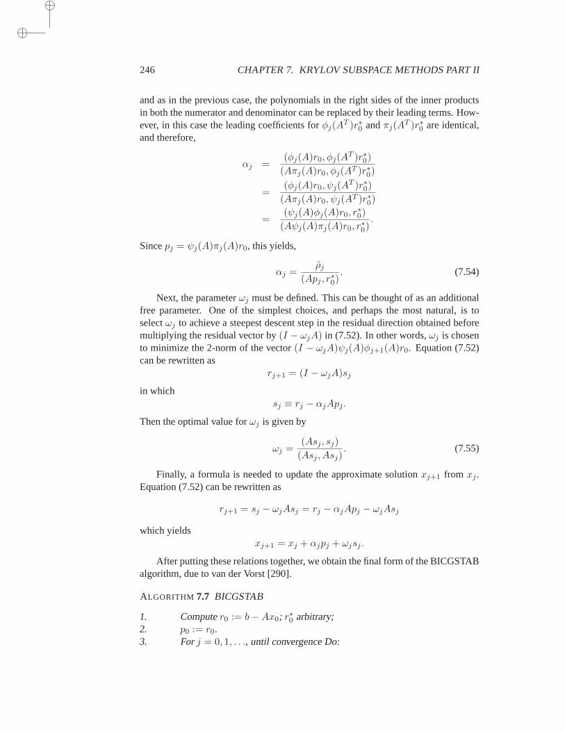
246 CHAPTER 7. KRYLOV SUBSPACE METHODS PART II
and as in the previous case, the polynomials in the right sides of the inner productsin both the numerator and denominator can be replaced by their leading terms. How-ever, in this case the leading coefficients forφj(A
T )r∗0 andπj(AT )r∗0 are identical,
and therefore,
αj =(φj(A)r0, φj(A
T )r∗0)(Aπj(A)r0, φj(AT )r∗0)
=(φj(A)r0, ψj(A
T )r∗0)(Aπj(A)r0, ψj(AT )r∗0)
=(ψj(A)φj(A)r0, r
∗0)
(Aψj(A)πj(A)r0, r∗0).
Sincepj = ψj(A)πj(A)r0, this yields,
αj =ρj
(Apj , r∗0). (7.54)
Next, the parameterωj must be defined. This can be thought of as an additionalfree parameter. One of the simplest choices, and perhaps the most natural, is toselectωj to achieve a steepest descent step in the residual direction obtained beforemultiplying the residual vector by(I − ωjA) in (7.52). In other words,ωj is chosento minimize the 2-norm of the vector(I − ωjA)ψj(A)φj+1(A)r0. Equation (7.52)can be rewritten as
rj+1 = (I − ωjA)sj
in whichsj ≡ rj − αjApj .
Then the optimal value forωj is given by
ωj =(Asj , sj)
(Asj , Asj). (7.55)
Finally, a formula is needed to update the approximate solutionxj+1 from xj .Equation (7.52) can be rewritten as
rj+1 = sj − ωjAsj = rj − αjApj − ωjAsj
which yieldsxj+1 = xj + αjpj + ωjsj .
After putting these relations together, we obtain the final form of the BICGSTABalgorithm, due to van der Vorst [290].
ALGORITHM 7.7 BICGSTAB
1. Computer0 := b−Ax0; r∗0 arbitrary;2. p0 := r0.3. Forj = 0, 1, . . ., until convergence Do:
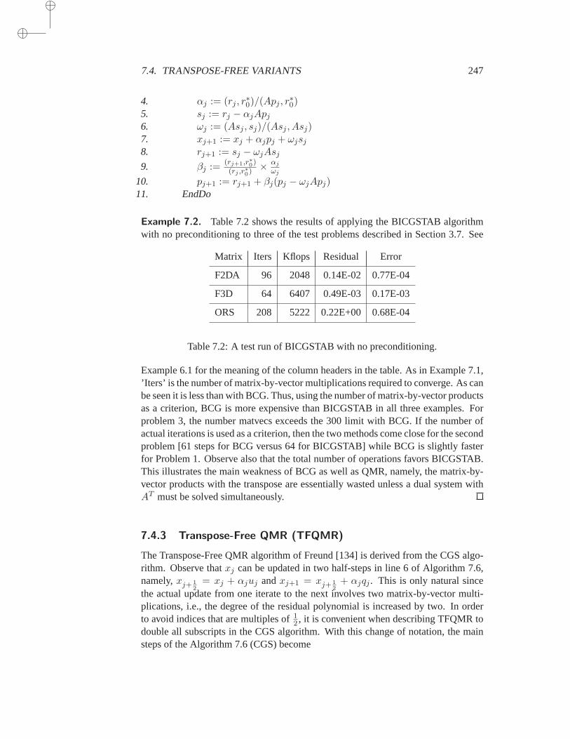
7.4. TRANSPOSE-FREE VARIANTS 247
4. αj := (rj , r∗0)/(Apj , r
∗0)
5. sj := rj − αjApj
6. ωj := (Asj , sj)/(Asj , Asj)7. xj+1 := xj + αjpj + ωjsj
8. rj+1 := sj − ωjAsj
9. βj :=(rj+1,r∗0)(rj ,r∗0) ×
αj
ωj
10. pj+1 := rj+1 + βj(pj − ωjApj)11. EndDo
Example 7.2. Table 7.2 shows the results of applying the BICGSTAB algorithmwith no preconditioning to three of the test problems described in Section 3.7. See
Matrix Iters Kflops Residual Error
F2DA 96 2048 0.14E-02 0.77E-04
F3D 64 6407 0.49E-03 0.17E-03
ORS 208 5222 0.22E+00 0.68E-04
Table 7.2: A test run of BICGSTAB with no preconditioning.
Example 6.1 for the meaning of the column headers in the table. As in Example 7.1,’Iters’ is the number of matrix-by-vector multiplications required to converge. As canbe seen it is less than with BCG. Thus, using the number of matrix-by-vector productsas a criterion, BCG is more expensive than BICGSTAB in all three examples.Forproblem 3, the number matvecs exceeds the 300 limit with BCG. If the number ofactual iterations is used as a criterion, then the two methods come close for the secondproblem [61 steps for BCG versus 64 for BICGSTAB] while BCG is slightly fasterfor Problem 1. Observe also that the total number of operations favors BICGSTAB.This illustrates the main weakness of BCG as well as QMR, namely, the matrix-by-vector products with the transpose are essentially wasted unless a dual system withAT must be solved simultaneously.
7.4.3 Transpose-Free QMR (TFQMR)
The Transpose-Free QMR algorithm of Freund [134] is derived fromthe CGS algo-rithm. Observe thatxj can be updated in two half-steps in line 6 of Algorithm 7.6,namely,xj+ 1
2= xj + αjuj andxj+1 = xj+ 1
2+ αjqj . This is only natural since
the actual update from one iterate to the next involves two matrix-by-vector multi-plications, i.e., the degree of the residual polynomial is increased by two. Inorderto avoid indices that are multiples of1
2 , it is convenient when describing TFQMR todouble all subscripts in the CGS algorithm. With this change of notation, the mainsteps of the Algorithm 7.6 (CGS) become
248 CHAPTER 7. KRYLOV SUBSPACE METHODS PART II
α2j = (r2j , r∗0)/(Ap2j , r
∗0) (7.56)
q2j = u2j − α2jAp2j (7.57)
x2j+2 = x2j + α2j(u2j + q2j) (7.58)
r2j+2 = r2j − α2jA(u2j + q2j) (7.59)
β2j = (r2j+2, r∗0)/(r2j , r
∗0) (7.60)
u2j+2 = r2j+2 + β2jq2j (7.61)
p2j+2 = u2j+2 + β2j(q2j + βp2j). (7.62)
The initialization is identical with that of Algorithm 7.6. The update of the ap-proximate solution in (7.58) can now be split into the following two half-steps:
x2j+1 = x2j + α2ju2j (7.63)
x2j+2 = x2j+1 + α2jq2j . (7.64)
This can be simplified by defining the vectorsum for oddm asu2j+1 = q2j . Simi-larly, the sequence ofαm is defined for odd values ofm asα2j+1 = α2j . In summary,
for m odd define:
um ≡ qm−1
αm ≡ αm−1. (7.65)
With these definitions, the relations (7.63–7.64) are translated into the single equation
xm = xm−1 + αm−1um−1,
which is valid whetherm is even or odd. The intermediate iteratesxm, withm odd,which are now defined do not exist in the original CGS algorithm. For even valuesof m the sequencexm represents the original sequence or iterates from the CGSalgorithm. It is convenient to introduce theN ×m matrix,
Um = [u0, . . . , um−1]
and them-dimensional vector
zm = (α0, α1, . . . , αm−1)T .
The general iteratexm satisfies the relation
xm = x0 + Umzm (7.66)
= xm−1 + αm−1um−1. (7.67)
From the above equation, it is clear that the residual vectorsrm are related to theu-vectors by the relations
rm = r0 −AUmzm (7.68)
= rm−1 − αm−1Aum−1. (7.69)
7.4. TRANSPOSE-FREE VARIANTS 249
Next, a relation similar to the relation (6.7) seen for FOM and GMRES will beextracted using the matrixAUm. As a result of (7.69), the following relation holds:
Aui =1
αi(ri − ri+1) .
Translated in matrix form, this relation becomes
AUm = Rm+1Bm (7.70)
whereRk = [r0, r1, . . . , rk−1] (7.71)
and whereBm is the(m+ 1)×m matrix,
Bm =
1 0 . . . . . . 0
−1 1...
0 −1 1 . . ....
.. . . . ....
... −1 10 . . . −1
× diag
1
α0,
1
α1, . . .
1
αm−1
. (7.72)
The columns ofRm+1 can be rescaled, for example, to make each of them have a2-norm equal to one, by multiplyingRm+1 to the right by a diagonal matrix. Let thisdiagonal matrix be the inverse of the matrix
∆m+1 = diag [δ0, δ1, . . . , δm] .
Then,AUm = Rm+1∆
−1m+1∆m+1Bm. (7.73)
With this, equation (7.68) becomes
rm = r0 −AUmzm = Rm+1
[e1 − Bmzm
](7.74)
= Rm+1∆−1m+1
[δ0e1 −∆m+1Bmzm
]. (7.75)
By analogy with the GMRES algorithm, define
Hm ≡ ∆m+1Bm.
Similarly, defineHm to be the matrix obtained fromHm by deleting its last row. It iseasy to verify that the CGS iteratesxm (now defined for all integersm = 0, 1, 2, . . .)satisfy the same definition as FOM, i.e.,
xm = x0 + UmH−1m (δ0e1). (7.76)
It is also possible to extract a GMRES-like solution from the relations (7.73) and(7.75), similar to DQGMRES. In order to minimize the residual norm over the Krylovsubspace, the 2-norm of the right-hand side of (7.75) would have to be minimized,
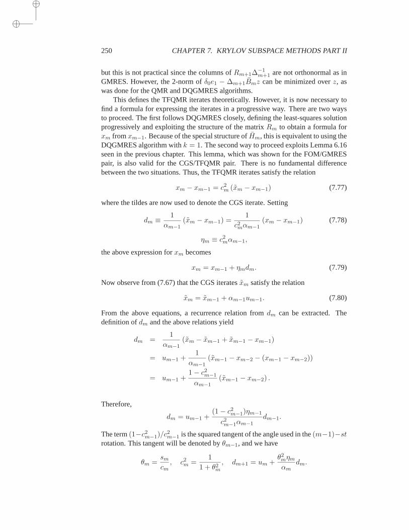
250 CHAPTER 7. KRYLOV SUBSPACE METHODS PART II
but this is not practical since the columns ofRm+1∆−1m+1 are not orthonormal as in
GMRES. However, the 2-norm ofδ0e1 − ∆m+1Bmz can be minimized overz, aswas done for the QMR and DQGMRES algorithms.
This defines the TFQMR iterates theoretically. However, it is now necessary tofind a formula for expressing the iterates in a progressive way. There are two waysto proceed. The first follows DQGMRES closely, defining the least-squares solutionprogressively and exploiting the structure of the matrixRm to obtain a formula forxm fromxm−1. Because of the special structure ofHm, this is equivalent to using theDQGMRES algorithm withk = 1. The second way to proceed exploits Lemma 6.16seen in the previous chapter. This lemma, which was shown for the FOM/GMRESpair, is also valid for the CGS/TFQMR pair. There is no fundamental differencebetween the two situations. Thus, the TFQMR iterates satisfy the relation
xm − xm−1 = c2m (xm − xm−1) (7.77)
where the tildes are now used to denote the CGS iterate. Setting
dm ≡1
αm−1(xm − xm−1) =
1
c2mαm−1(xm − xm−1) (7.78)
ηm ≡ c2mαm−1,
the above expression forxm becomes
xm = xm−1 + ηmdm. (7.79)
Now observe from (7.67) that the CGS iteratesxm satisfy the relation
xm = xm−1 + αm−1um−1. (7.80)
From the above equations, a recurrence relation fromdm can be extracted. Thedefinition ofdm and the above relations yield
dm =1
αm−1(xm − xm−1 + xm−1 − xm−1)
= um−1 +1
αm−1(xm−1 − xm−2 − (xm−1 − xm−2))
= um−1 +1− c2m−1
αm−1(xm−1 − xm−2) .
Therefore,
dm = um−1 +(1− c2m−1)ηm−1
c2m−1αm−1dm−1.
The term(1−c2m−1)/c2m−1 is the squared tangent of the angle used in the(m−1)−st
rotation. This tangent will be denoted byθm−1, and we have
θm =sm
cm, c2m =
1
1 + θ2m
, dm+1 = um +θ2mηm
αmdm.
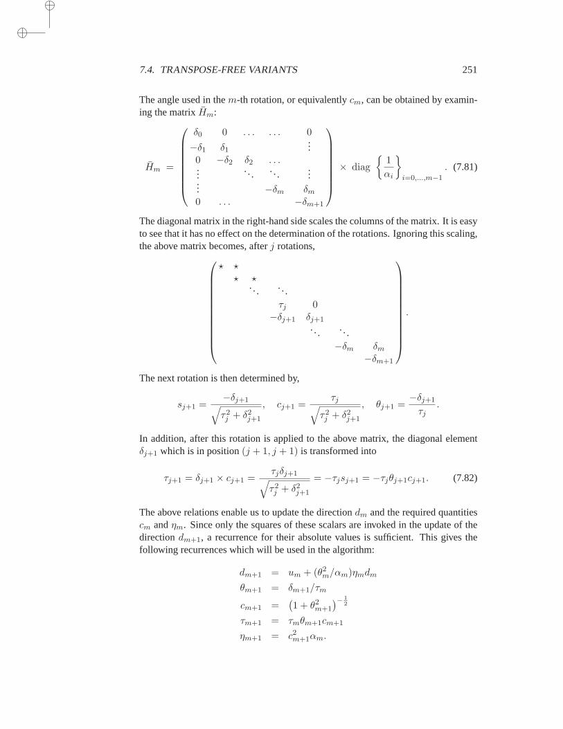
7.4. TRANSPOSE-FREE VARIANTS 251
The angle used in them-th rotation, or equivalentlycm, can be obtained by examin-ing the matrixHm:
Hm =
δ0 0 . . . . . . 0
−δ1 δ1...
0 −δ2 δ2 . . ....
. .. .. ....
... −δm δm0 . . . −δm+1
× diag
1
αi
i=0,...,m−1
. (7.81)
The diagonal matrix in the right-hand side scales the columns of the matrix. It is easyto see that it has no effect on the determination of the rotations. Ignoring thisscaling,the above matrix becomes, afterj rotations,
⋆ ⋆⋆ ⋆
. .. . ..τj 0−δj+1 δj+1
. . . . ..−δm δm
−δm+1
.
The next rotation is then determined by,
sj+1 =−δj+1
√
τ2j + δ2j+1
, cj+1 =τj
√
τ2j + δ2j+1
, θj+1 =−δj+1
τj.
In addition, after this rotation is applied to the above matrix, the diagonal elementδj+1 which is in position(j + 1, j + 1) is transformed into
τj+1 = δj+1 × cj+1 =τjδj+1
√
τ2j + δ2j+1
= −τjsj+1 = −τjθj+1cj+1. (7.82)
The above relations enable us to update the directiondm and the required quantitiescm andηm. Since only the squares of these scalars are invoked in the update of thedirectiondm+1, a recurrence for their absolute values is sufficient. This gives thefollowing recurrences which will be used in the algorithm:
dm+1 = um + (θ2m/αm)ηmdm
θm+1 = δm+1/τm
cm+1 =(1 + θ2
m+1
)− 12
τm+1 = τmθm+1cm+1
ηm+1 = c2m+1αm.

252 CHAPTER 7. KRYLOV SUBSPACE METHODS PART II
Before writing down the algorithm, a few relations must be exploited. Since thevectorsrm are no longer the actual residuals in the algorithm, we change the notationtowm. These residual vectors can be updated by the formula
wm = wm−1 − αm−1Aum−1.
The vectorsAui can be used to update the vectors
v2j ≡ Ap2j
which are needed in the CGS algorithm. Multiplying (7.62) byA results in
Ap2j = Au2j + β2j−2(Aq2j−2 + βjAp2j−2)
which, upon substituting the relation
q2j = u2j+1
translates intov2j = Au2j + β2j−2(Au2j−1 + β2j−2v2j−2).
Also, observe that the recurrences in (7.57) and (7.61) forq2j andu2j+2, respectively,become
u2j+1 = u2j − α2jv2j
u2j+2 = w2j+2 + β2ju2j+1.
The first equation should be used to computeum+1 whenm is even, and the secondwhenm is odd. In the following algorithm, the normalizationδm = ‖wm‖2, whichnormalize each column ofRm to have 2-norm unity, is used.
ALGORITHM 7.8 Transpose-Free QMR (TFQMR)
1. Computew0 = u0 = r0 = b−Ax0, v0 = Au0, d0 = 0;2. τ0 = ‖r0‖2, θ0 = η0 = 0.3. Chooser∗0 such thatρ0 ≡ (r∗0, r0) 6= 0.4. Form = 0, 1, 2, . . . , until convergence Do:5. If m is even then6. αm+1 = αm = ρm/(vm, r
∗0)
7. um+1 = um − αmvm
8. EndIf9. wm+1 = wm − αmAum
10. dm+1 = um + (θ2m/αm)ηmdm
11. θm+1 = ‖wm+1‖2/τm; cm+1 =(1 + θ2
m+1
)− 12
12. τm+1 = τmθm+1cm+1 ; ηm+1 = c2m+1αm
13. xm+1 = xm + ηm+1dm+1
14. Ifm is odd then
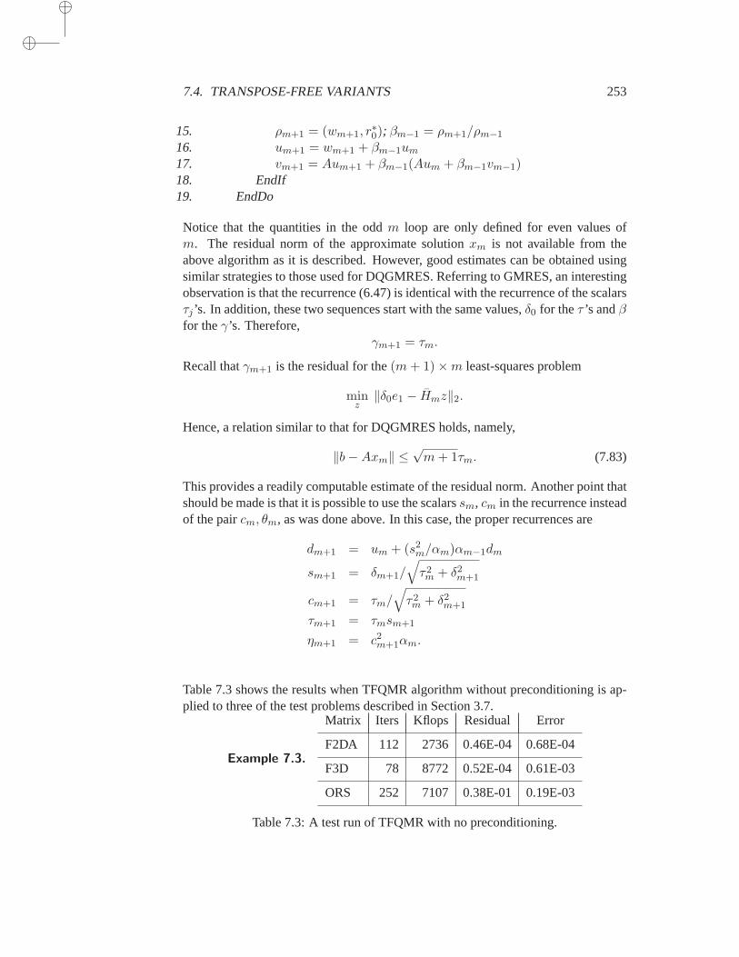
7.4. TRANSPOSE-FREE VARIANTS 253
15. ρm+1 = (wm+1, r∗0); βm−1 = ρm+1/ρm−1
16. um+1 = wm+1 + βm−1um
17. vm+1 = Aum+1 + βm−1(Aum + βm−1vm−1)18. EndIf19. EndDo
Notice that the quantities in the oddm loop are only defined for even values ofm. The residual norm of the approximate solutionxm is not available from theabove algorithm as it is described. However, good estimates can be obtained usingsimilar strategies to those used for DQGMRES. Referring to GMRES, an interestingobservation is that the recurrence (6.47) is identical with the recurrenceof the scalarsτj ’s. In addition, these two sequences start with the same values,δ0 for theτ ’s andβfor theγ’s. Therefore,
γm+1 = τm.
Recall thatγm+1 is the residual for the(m+ 1)×m least-squares problem
minz‖δ0e1 − Hmz‖2.
Hence, a relation similar to that for DQGMRES holds, namely,
‖b−Axm‖ ≤√m+ 1τm. (7.83)
This provides a readily computable estimate of the residual norm. Another point thatshould be made is that it is possible to use the scalarssm, cm in the recurrence insteadof the paircm, θm, as was done above. In this case, the proper recurrences are
dm+1 = um + (s2m/αm)αm−1dm
sm+1 = δm+1/√
τ2m + δ2m+1
cm+1 = τm/√
τ2m + δ2m+1
τm+1 = τmsm+1
ηm+1 = c2m+1αm.
Table 7.3 shows the results when TFQMR algorithm without preconditioning is ap-plied to three of the test problems described in Section 3.7.
Example 7.3.
Matrix Iters Kflops Residual Error
F2DA 112 2736 0.46E-04 0.68E-04
F3D 78 8772 0.52E-04 0.61E-03
ORS 252 7107 0.38E-01 0.19E-03
Table 7.3: A test run of TFQMR with no preconditioning.
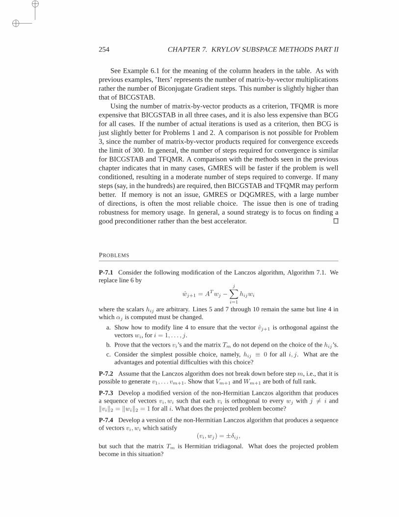
254 CHAPTER 7. KRYLOV SUBSPACE METHODS PART II
See Example 6.1 for the meaning of the column headers in the table. As withprevious examples, ’Iters’ represents the number of matrix-by-vector multiplicationsrather the number of Biconjugate Gradient steps. This number is slightly higher thanthat of BICGSTAB.
Using the number of matrix-by-vector products as a criterion, TFQMR is moreexpensive that BICGSTAB in all three cases, and it is also less expensive than BCGfor all cases. If the number of actual iterations is used as a criterion, thenBCG isjust slightly better for Problems 1 and 2. A comparison is not possible for Problem3, since the number of matrix-by-vector products required for convergence exceedsthe limit of 300. In general, the number of steps required for convergence is similarfor BICGSTAB and TFQMR. A comparison with the methods seen in the previouschapter indicates that in many cases, GMRES will be faster if the problem is wellconditioned, resulting in a moderate number of steps required to converge.If manysteps (say, in the hundreds) are required, then BICGSTAB and TFQMRmay performbetter. If memory is not an issue, GMRES or DQGMRES, with a large numberof directions, is often the most reliable choice. The issue then is one of tradingrobustness for memory usage. In general, a sound strategy is to focus on finding agood preconditioner rather than the best accelerator.
PROBLEMS
P-7.1 Consider the following modification of the Lanczos algorithm, Algorithm 7.1. Wereplace line 6 by
wj+1 = ATwj −j∑
i=1
hijwi
where the scalarshij are arbitrary. Lines 5 and 7 through 10 remain the same but line 4 inwhichαj is computed must be changed.
a. Show how to modify line 4 to ensure that the vectorvj+1 is orthogonal against thevectorswi, for i = 1, . . . , j.
b. Prove that the vectorsvi’s and the matrixTm do not depend on the choice of thehij ’s.
c. Consider the simplest possible choice, namely,hij ≡ 0 for all i, j. What are theadvantages and potential difficulties with this choice?
P-7.2 Assume that the Lanczos algorithm does not break down beforestepm, i.e., that it ispossible to generatev1, . . . vm+1. Show thatVm+1 andWm+1 are both of full rank.
P-7.3 Develop a modified version of the non-Hermitian Lanczos algorithm that producesa sequence of vectorsvi, wi such that eachvi is orthogonal to everywj with j 6= i and‖vi‖2 = ‖wi‖2 = 1 for all i. What does the projected problem become?
P-7.4 Develop a version of the non-Hermitian Lanczos algorithm that produces a sequenceof vectorsvi, wi which satisfy
(vi, wj) = ±δij ,but such that the matrixTm is Hermitian tridiagonal. What does the projected problembecome in this situation?

7.4. TRANSPOSE-FREE VARIANTS 255
P-7.5 Using the notation of Section 7.1.2 prove thatqj+k(t) = tkpj(t) is orthogonal tothe polynomialsp1, p2, . . . , pj−k, assuming thatk ≤ j. Show that ifqj+k is orthogonalizedagainstp1, p2, . . . , pj−k, the result would be orthogonal to all polynomials of degree< j+k.Derive a general Look-Ahead non-Hermitian Lanczos procedure based on this observation.
P-7.6 Consider the matricesVm = [v1, . . . , vm] andWm = [w1, . . . , wm] obtained fromthe Lanczos biorthogonalization algorithm. (a) What are thematrix representations of the(oblique) projector ontoKm(A, v1) orthogonal to the subspaceKm(AT , w1), and the pro-jector ontoKm(AT , w1) orthogonally to the subspaceKm(A, v1)? (b) Express a generalcondition for the existence of an oblique projector ontoK, orthogonal toL. (c) How can thiscondition be interpreted using the Lanczos vectors and the Lanczos algorithm?
P-7.7 Show a three-term recurrence satisfied by the residual vectors rj of the BCG algo-rithm. Include the first two iterates to start the recurrence. Similarly, establish a three-termrecurrence for the conjugate direction vectorspj in BCG.
P-7.8 Let φj(t) andπj(t) be the residual polynomial and the conjugate direction polyno-mial, respectively, for the BCG algorithm, as defined in Section 7.4.1. Letψj(t) be any otherpolynomial sequence which is defined from the recurrence
ψ0(t) = 1, ψ1(t) = (1− ξ0t)ψ0(t)
ψj+1(t) = (1 + ηj − ξjt)ψj(t)− ηjψj−1(t)
a. Show that the polynomialsψj are consistent, i.e.,ψj(0) = 1 for all j ≥ 0.
b. Show the following relations
ψj+1φj+1 = ψjφj+1 − ηj(ψj−1 − ψj)φj+1 − ξjtψjφj+1
ψjφj+1 = ψjφj − αjtψjπj
(ψj−1 − ψj)φj+1 = ψj−1φj − ψjφj+1 − αjtψj−1πj
ψj+1πj+1 = ψj+1φj+1 − βjηjψj−1πj + βj(1 + ηj)ψjπj − βjξjtψjπj
ψjπj+1 = ψjφj+1 + βjψjπj .
c. Defining,
tj = ψj(A)φj+1(A)r0, yj = (ψj−1(A)− ψj(A))φj+1(A)r0,pj = ψj(A)πj(A)r0, sj = ψj−1(A)πj(A)r0
show how the recurrence relations of the previous question translate for these vectors.
d. Find a formula that allows one to update the approximationxj+1 from the vectorsxj−1, xj andtj , pj , yj , sj defined above.
e. Proceeding as in BICGSTAB, find formulas for generating the BCG coefficientsαj
andβj from the vectors defined in the previous question.
P-7.9 Prove the expression (7.76) for the CGS approximation defined by (7.66–7.67). Isthe relation valid for any choice of scaling∆m+1?
P-7.10 Prove that the vectorsrj andr∗i produced by the BCG algorithm are orthogonal toeach other wheni 6= j, while the vectorspi andp∗j areA-orthogonal, i.e.,(Apj , p
∗i ) = 0 for
i 6= j.
P-7.11 The purpose of this exercise is to develop block variants of the Lanczos algorithm.Consider a two-sided analogue of the Block-Arnoldi algorithm, in its variant of Algorithm6.24. Formally, the general step that defines the biorthogonalization process, forj ≥ p, is asfollows:
256 CHAPTER 7. KRYLOV SUBSPACE METHODS PART II
1. OrthogonalizeAvj−p+1 versusw1, w2, . . . , wj (by subtracting a linear combinationof v1, . . . , vj fromAvj−p+1). Call v the resulting vector.
2. OrthogonalizeATwj−p+1 versusv1, v2, . . . , vj (by subtracting a linear combinationof w1, . . . , wj fromATwj−p+1). Callw the resulting vector.
3. Normalize the two vectorsv andw so that(v, w) = 1 to getvj+1 andwj+1.
Here,p is the block size and it is assumed that the initial blocks arebiorthogonal:(vi, wj) =δij for i, j ≤ p.
a. Show thatAvj−p+1 needs only to be orthogonalized against the2p previouswi’s in-stead of all of them. Similarly,ATwj−p+1 must be orthogonalized only against the2ppreviousvi’s.
b. Write down the algorithm completely. Show the orthogonality relations satisfied bythe vectorsvi andwj . Show also relations similar to (7.3) and (7.4).
c. We now assume that the two sets of vectorsvi andwj have different block sizes. Callq the block-size for thew’s. Line 2 of the above formal algorithm is changed into:
2a. OrthogonalizeATwj−q+1 versusv1, v2, . . . , vj (· · ·). Callw the resulting vector.
and the rest remains unchanged. The initial vectors are again biorthogonal:(vi, wj) =δij for i ≤ p andj ≤ q. Show that nowAvj−p+1 needs only to be orthogonalizedagainst theq+p previouswi’s instead of all of them. Show a simlar result for thewj ’s.
d. Show how a block version of BCG and QMR can be developed based on the algorithmresulting from question (c).
NOTES AND REFERENCES. The pioneering paper by Lanczos [197], on what is now referred toasBi-CG, did not receive the attention it deserved. Fletcher [130] who developed the modern version ofthe algorithm mentions the 1950 Lanczos paper [195] which is devoted mostly to eigenvalue problems,but seemed unaware of the second [197] which is devoted to linear systems. Likewise, the paper bySonneveld [272] which proved for the first time that theAT operations were not necessary, receivedlittle attention for several years (the first reference to the method [312] dates back to 1980). TFQMR(Freund and Nachtigal [136]) and BICGSTAB (van der Vorst [290]) were later developed to curesome of the numerical problems that plague CGS. Many additions and variations to the basic BCG,BICGSTAB, and TFQMR techniques appeared, see, e.g., [63, 72, 160, 161, 260], among others. Somevariations were developed to cope with the breakdown of the underlying Lanczos or BCG algorithm;see, for example, [62, 27, 135, 260, 321]. Finally, block methods ofthese algorithms have also beendeveloped, see, e.g., [5].
The Lanczos-type algorithms developed for solving linear systems are rooted in the theory oforthogonal polynomials and Pade approximation. Lanczos himself certainly used this viewpoint whenhe wrote his breakthrough papers [195, 197] in the early 1950s. The monograph by Brezinski [59]gives an excellent coverage of the intimate relations between approximation theory and the Lanczos-type algorithms. Freund [133] establishes these relations for quasi-minimal residual methods. A fewoptimality properties for the class of methods presented in this chapter can be proved using a variablemetric, i.e., an inner product which is different at each step [29]. A survey by Weiss [308] presents aframework for Krylov subspace methods explaining some of these optimality properties and the inter-relationships between Krylov subspace methods. Several authors discuss a class of techniques knownas residual smoothing; see for example [259, 324, 308, 61]. Thesetechniques can be applied to anyiterative sequencexk to build a new sequence of iteratesyk by combiningyk−1 with the differencexk − yk−1. A remarkable result shown by Zhou and Walker [324] is that the iteratesof the QMRalgorithm can be obtained from those of the BCG as a particular case of residual smoothing.
7.4. TRANSPOSE-FREE VARIANTS 257
A number of projection-type methods on Krylov subspaces, other than those seen in this chapterand the previous one are described in [1]. The group of rank-k update methods discussed by Eirolaand Nevanlinna [113] and Deuflhard et al. [100] is closely related to Krylov subspace methods. Infact, GMRES can be viewed as a particular example of these methods. Alsoof interest and notcovered in this book are thevector extrapolationtechniques which are discussed, for example, in thebooks Brezinski [59], Brezinski and Radivo Zaglia [60] and the articles [270] and [177]. Connectionsbetween these methods and Krylov subspace methods, have been uncovered, and are discussed byBrezinski [59] and Sidi [263].

258 CHAPTER 7. KRYLOV SUBSPACE METHODS PART II
Chapter 8
METHODS RELATED TO THE NORMAL
EQUATIONS
There are a number of techniques for converting a non-symmetric linear system into a symmetric
one. One such technique solves the equivalent linear system AT Ax = AT b, called the normal
equations. Often, this approach is avoided in practice because the coefficient matrix AT A is
much worse conditioned than A. However, the normal equations approach may be adequate in
some situations. Indeed, there are even applications in which it is preferred to the usual Krylov
subspace techniques. This chapter covers iterative methods which are either directly or implicitly
related to the normal equations.
8.1 The Normal Equations
In order to solve the linear systemAx = b whenA is nonsymmetric, we can solvethe equivalent system
ATA x = AT b (8.1)
which is Symmetric Positive Definite. This system is known as the system of thenormal equationsassociated with the least-squares problem,
minimize ‖b−Ax‖2. (8.2)
Note that (8.1) is typically used to solve the least-squares problem (8.2) forover-determinedsystems, i.e., whenA is a rectangular matrix of sizen×m,m < n.
A similar well known alternative setsx = ATu and solves the following equationfor u:
AATu = b. (8.3)
Once the solutionu is computed, the original unknownx could be obtained by mul-tiplying u byAT . However, most of the algorithms we will see do not invoke theuvariable explicitly and work with the original variablex instead. The above systemof equations can be used to solveunder-determinedsystems, i.e., those systems in-volving rectangular matrices of sizen×m, with n < m. It is related to (8.1) in thefollowing way. Assume thatn ≤ m and thatA has full rank. Letx∗ beanysolutionto the underdetermined systemAx = b. Then (8.3) represents the normal equationsfor the least-squares problem,
minimize ‖x∗ −ATu‖2. (8.4)
259
260 CHAPTER 8. METHODS RELATED TO THE NORMAL EQUATIONS
Since by definitionATu = x, then (8.4) will find the solution vectorx that is closestto x∗ in the 2-norm sense. What is interesting is that whenn < m there are infinitelymany solutionsx∗ to the systemAx = b, but the minimizeru of (8.4) does notdepend on the particularx∗ used.
The system (8.1) and methods derived from it are often labeled with NR (Nfor “Normal” and R for “Residual”) while (8.3) and related techniques arelabeledwith NE (N for “Normal” and E for “Error”). If A is square and nonsingular, thecoefficient matrices of these systems are both Symmetric Positive Definite, andthesimpler methods for symmetric problems, such as the Conjugate Gradient algorithm,can be applied. Thus, CGNE denotes the Conjugate Gradient method appliedto thesystem (8.3) and CGNR the Conjugate Gradient method applied to (8.1).
There are several alternative ways to formulate symmetric linear systems havingthe same solution as the original system. For instance, the symmetric linear system
(I AAT O
)(rx
)
=
(b0
)
(8.5)
with r = b − Ax, arises from the standard necessary conditions satisfied by thesolution of the constrained optimization problem,
minimize1
2‖r − b‖22 (8.6)
subject toAT r = 0. (8.7)
The solutionx to (8.5) is the vector of Lagrange multipliers for the above problem.Another equivalent symmetric system is of the form
(O AAT O
)(Axx
)
=
(b
AT b
)
.
The eigenvalues of the coefficient matrix for this system are±σi, whereσi is anarbitrary singular value ofA. Indefinite systems of this sort are not easier to solvethan the original nonsymmetric system in general. Although not obvious immedi-ately, this approach is similar in nature to the approach (8.1) and the correspondingConjugate Gradient iterations applied to them should behave similarly.
A general consensus is that solving the normal equations can be an inefficientapproach in the case whenA is poorly conditioned. Indeed, the 2-norm conditionnumber ofATA is given by
Cond2(ATA) = ‖ATA‖2 ‖(ATA)−1‖2.
Now observe that‖ATA‖2 = σ2max(A) whereσmax(A) is the largest singular value
of A which, incidentally, is also equal to the 2-norm ofA. Thus, using a similarargument for the inverse(ATA)−1 yields
Cond2(ATA) = ‖A‖22 ‖A−1‖22 = Cond2
2(A). (8.8)
The 2-norm condition number forATA is exactly the square of the condition numberof A, which could cause difficulties. For example, if originallyCond2(A) = 108,
8.2. ROW PROJECTION METHODS 261
then an iterative method may be able to perform reasonably well. However, acon-dition number of1016 can be much more difficult to handle by a standard iterativemethod. That is because any progress made in one step of the iterative proceduremay be annihilated by the noise due to numerical errors.
On the other hand, if the original matrix has a good 2-norm condition number,then the normal equation approach should not cause any serious difficulties. In theextreme case whenA is unitary, i.e., whenAHA = I, then the normal equationsare clearly the best approach (the Conjugate Gradient method will converge in zerostep!).
8.2 Row Projection Methods
When implementing a basic relaxation scheme, such as Jacobi or SOR, to solvethelinear system
ATAx = AT b, (8.9)
orAATu = b, (8.10)
it is possible to exploit the fact that the matricesATA or AAT need not be formedexplicitly. As will be seen, only a row or a column ofA at a time is needed at a givenrelaxation step. These methods are known asrow projection methodssince they areindeed projection methods on rows ofA or AT . Block row projection methods canalso be defined similarly.
8.2.1 Gauss-Seidel on the Normal Equations
It was stated above that in order to use relaxation schemes on the normal equations,only access to one column ofA at a time is needed for (8.9) and one row at a timefor (8.10). This is now explained for (8.10) first. Starting from an approximationto the solution of (8.10), a basic relaxation-based iterative procedure modifies itscomponents in a certain order using a succession of relaxation steps of thesimpleform
unew = u+ δiei (8.11)
whereei is thei-th column of the identity matrix. The scalarδi is chosen so that thei-th component of the residual vector for (8.10) becomes zero. Therefore,
(b−AAT (u+ δiei), ei) = 0 (8.12)
which, settingr = b−AATu, yields,
δi =(r, ei)
‖AT ei‖22. (8.13)
Denote byβi thei-th component ofb. Then a basic relaxation step consists of taking
δi =βi − (ATu,AT ei)
‖AT ei‖22. (8.14)
262 CHAPTER 8. METHODS RELATED TO THE NORMAL EQUATIONS
Also, (8.11) can be rewritten in terms ofx-variables as follows:
xnew = x+ δiAT ei. (8.15)
The auxiliary variableu has now been removed from the scene and is replaced bythe original variablex = ATu.
Consider the implementation of a forward Gauss-Seidel sweep based on (8.15)and (8.13) for a general sparse matrix. The evaluation ofδi from (8.13) requires theinner product of the current approximationx = ATu with AT ei, thei-th row ofA.This inner product is inexpensive to compute becauseAT ei is usually sparse. If anacceleration parameterω is used, we only need to changeδi into ωδi. Therefore, aforward SOR sweep would be as follows.
ALGORITHM 8.1 Forward NE-SOR Sweep
1. Choose an initialx.2. Fori = 1, 2, . . . , n Do:
3. δi = ω βi−(AT ei,x)‖AT ei‖2
2
4. x := x+ δiAT ei
5. EndDo
Note thatAT ei is a vector equal to the transpose of thei-th row ofA. All that isneeded is the row data structure forA to implement the above algorithm. Denotingby nzi the number of nonzero elements in thei-th row ofA, then each step of theabove sweep requires2nzi + 2 operations in line 3, and another2nzi operations inline 4, bringing the total to4nzi +2. The total for a whole sweep becomes4nz+2noperations, wherenz represents the total number of nonzero elements ofA. Twice asmany operations are required for the Symmetric Gauss-Seidel or the SSOR iteration.Storage consists of the right-hand side, the vectorx, and possibly an additional vectorto store the 2-norms of the rows ofA. A better alternative would be to rescale eachrow by its 2-norm at the start.
Similarly, Gauss-Seidel for (8.9) would consist of a sequence of steps of the form
xnew = x+ δiei. (8.16)
Again, the scalarδi is to be selected so that thei-th component of the residual vectorfor (8.9) becomes zero, which yields
(AT b−ATA(x+ δiei), ei) = 0. (8.17)
With r ≡ b−Ax, this becomes(AT (r − δiAei), ei) = 0, which yields
δi =(r,Aei)
‖Aei‖22. (8.18)
Then the following algorithm is obtained.
8.2. ROW PROJECTION METHODS 263
ALGORITHM 8.2 Forward NR-SOR Sweep
1. Choose an initialx, computer := b−Ax.2. Fori = 1, 2, . . . , n Do:3. δi = ω (r,Aei)
‖Aei‖22
4. x := x+ δiei5. r := r − δiAei6. EndDo
In contrast with Algorithm 8.1, the column data structure ofA is now needed forthe implementation instead of its row data structure. Here, the right-hand sideb canbe overwritten by the residual vectorr, so the storage requirement is essentially thesame as in the previous case. In the NE version, the scalarβi− (x, ai) is just thei-thcomponent of the current residual vectorr = b − Ax. As a result, stopping criteriacan be built for both algorithms based on either the residual vector or the variationin the solution. Note that the matricesAAT andATA can be dense or generallymuch less sparse thanA, yet the cost of the above implementations depends onlyon the nonzero structure ofA. This is a significant advantage of relaxation-typepreconditioners over incomplete factorization preconditioners when usingConjugateGradient methods to solve the normal equations.
One question remains concerning the acceleration of the above relaxation schemesby under- or over-relaxation. If the usual acceleration parameterω is introduced, thenwe only have to multiply the scalarsδi in the previous algorithms byω. One seriousdifficulty here is to determine the optimal relaxation factor. If nothing in particu-lar is known about the matrixAAT , then the method will converge for anyω lyingstrictly between0 and2, as was seen in Chapter 4, because the matrix is positive def-inite. Moreover, another unanswered question is how convergence can be affectedby various reorderings of the rows. For general sparse matrices, theanswer is notknown.
8.2.2 Cimmino’s Method
In a Jacobi iteration for the system (8.9), the components of the new iterate satisfythe following condition:
(AT b−ATA(x+ δiei), ei) = 0. (8.19)
This yields
(b−A(x+ δiei), Aei) = 0 or (r − δiAei, Aei) = 0
in whichr is the old residualb−Ax. As a result, thei-component of the new iteratexnew is given by
xnew,i = xi + δiei, (8.20)
δi =(r,Aei)
‖Aei‖22. (8.21)
264 CHAPTER 8. METHODS RELATED TO THE NORMAL EQUATIONS
Here, be aware that these equations do not result in the same approximationas thatproduced by Algorithm 8.2, even though the modifications are given by the sameformula. Indeed, the vectorx is not updated after each step and therefore the scalarsδi are different for the two algorithms. This algorithm is usually described with anacceleration parameterω, i.e., all δi’s are multiplied uniformly by a certainω. If ddenotes the vector with coordinatesδi, i = 1, . . . , n, the following algorithm results.
ALGORITHM 8.3 Cimmino-NR
1. Choose initial guessx0. Setx = x0, r = b−Ax0
2. Until convergence Do:3. Fori = 1, . . . , n Do:4. δi = ω (r,Aei)
‖Aei‖22
5. EndDo6. x := x+ d whered =
∑ni=1 δiei
7. r := r −Ad8. EndDo
Notice that all the coordinates will use the same residual vectorr to computethe updatesδi. Whenω = 1, each instance of the above formulas is mathematicallyequivalent to performing a projection step for solvingAx = b with K = spanei,andL = AK. It is also mathematically equivalent to performing an orthogonalprojection step for solvingATAx = AT b with K = spanei.
It is interesting to note that when each columnAei is normalized by its 2-norm,i.e., if ‖Aei‖2 = 1, i = 1, . . . , n, thenδi = ω(r,Aei) = ω(AT r, ei). In this situation,
d = ωAT r = ωAT (b−Ax)
and the main loop of the algorithm takes the vector form
d := ωAT r
x := x+ d
r := r −Ad.
Each iteration is therefore equivalent to a step of the form
xnew = x+ ω(AT b−ATAx
)
which is nothing but the Richardson iteration applied to the normal equations (8.1).In particular, as was seen in Example 4.1, convergence is guaranteed for anyω whichsatisfies,
0 < ω <2
λmax(8.22)
whereλmax is the largest eigenvalue ofATA. In addition, the best accelerationparameter is given by
ωopt =2
λmin + λmax
8.2. ROW PROJECTION METHODS 265
in which, similarly,λmin is the smallest eigenvalue ofATA. If the columns are notnormalized by their 2-norms, then the procedure is equivalent to a preconditionedRichardson iteration with diagonal preconditioning. The theory regardingconver-gence is similar but involves the preconditioned matrix or, equivalently, the matrixA′ obtained fromA by normalizing its columns.
The algorithm can be expressed in terms of projectors. Observe that the newresidual satisfies
rnew = r −n∑
i=1
ω(r,Aei)
‖Aei‖22Aei. (8.23)
Each of the operators
Pi : r −→ (r,Aei)
‖Aei‖22Aei ≡ Pir (8.24)
is an orthogonal projector ontoAei, thei-th column ofA. Hence, we can write
rnew =
(
I − ωn∑
i=1
Pi
)
r. (8.25)
There are two important variations to the above scheme. First, because the pointJacobi iteration can be very slow, it may be preferable to work with sets of vectorsinstead. Letπ1, π2, . . . , πp be a partition of the set1, 2, . . . , n and, for eachπj ,letEj be the matrix obtained by extracting the columns of the identity matrix whoseindices belong toπj . Going back to the projection framework, defineAi = AEi. Ifan orthogonal projection method is used ontoEj to solve (8.1), then the new iterateis given by
xnew = x+ ω
p∑
i
Eidi (8.26)
di = (ETi A
TAEi)−1ET
i AT r = (AT
i Ai)−1AT
i r. (8.27)
Each individual block-componentdi can be obtained by solving a least-squares prob-lem
mind‖r −Aid‖2.
An interpretation of this indicates that each individual substep attempts to reduce theresidual as much as possible by taking linear combinations from specific columns ofAi. Similar to the scalar iteration, we also have
rnew =
(
I − ωn∑
i=1
Pi
)
r
wherePi now represents an orthogonal projector onto the span ofAi.Note thatA1, A2, . . . , Ap is a partition of the column-setAeii=1,...,n and this
partition can be arbitrary. Another remark is that the original Cimmino method wasformulated for rows instead of columns, i.e., it was based on (8.1) instead of(8.3).The alternative algorithm based on columns rather than rows is easy to derive.
266 CHAPTER 8. METHODS RELATED TO THE NORMAL EQUATIONS
8.3 Conjugate Gradient and Normal Equations
A popular combination to solve nonsymmetric linear systems applies the ConjugateGradient algorithm to solve either (8.1) or (8.3). As is shown next, the resulting algo-rithms can be rearranged because of the particular nature of the coefficient matrices.
8.3.1 CGNR
We begin with the Conjugate Gradient algorithm applied to (8.1). Applying CGdirectly to the system and denoting byzi the residual vector at stepi (instead ofri)results in the following sequence of operations:
• αj := (zj , zj)/(ATApj , pj) = (zj , zj)/(Apj , Apj)
• xj+1 := xj + αjpj
• zj+1 := zj − αjATApj
• βj := (zj+1, zj+1)/(zj , zj)
• pj+1 := zj+1 + βjpj .
If the original residualri = b−Axi must be available at every step, we may computethe residualzi+1 in two parts:rj+1 := rj − αjApj and thenzi+1 = AT ri+1 whichis the residual for the normal equations (8.1). It is also convenient to introduce thevectorwi = Api. With these definitions, the algorithm can be cast in the followingform.
ALGORITHM 8.4 CGNR
1. Computer0 = b−Ax0, z0 = AT r0, p0 = z0.2. Fori = 0, . . ., until convergence Do:3. wi = Api
4. αi = ‖zi‖2/‖wi‖225. xi+1 = xi + αipi
6. ri+1 = ri − αiwi
7. zi+1 = AT ri+1
8. βi = ‖zi+1‖22/‖zi‖22,9. pi+1 = zi+1 + βipi
10. EndDo
In Chapter 6, the approximationxm produced at them-th step of the ConjugateGradient algorithm was shown to minimize the energy norm of the error over anaffine Krylov subspace. In this case,xm minimizes the function
f(x) ≡ (ATA(x∗ − x), (x∗ − x))
over all vectorsx in the affine Krylov subspace
x0 +Km(ATA,AT r0) = x0 + spanAT r0, ATAAT r0, . . . , (A
TA)m−1AT r0,
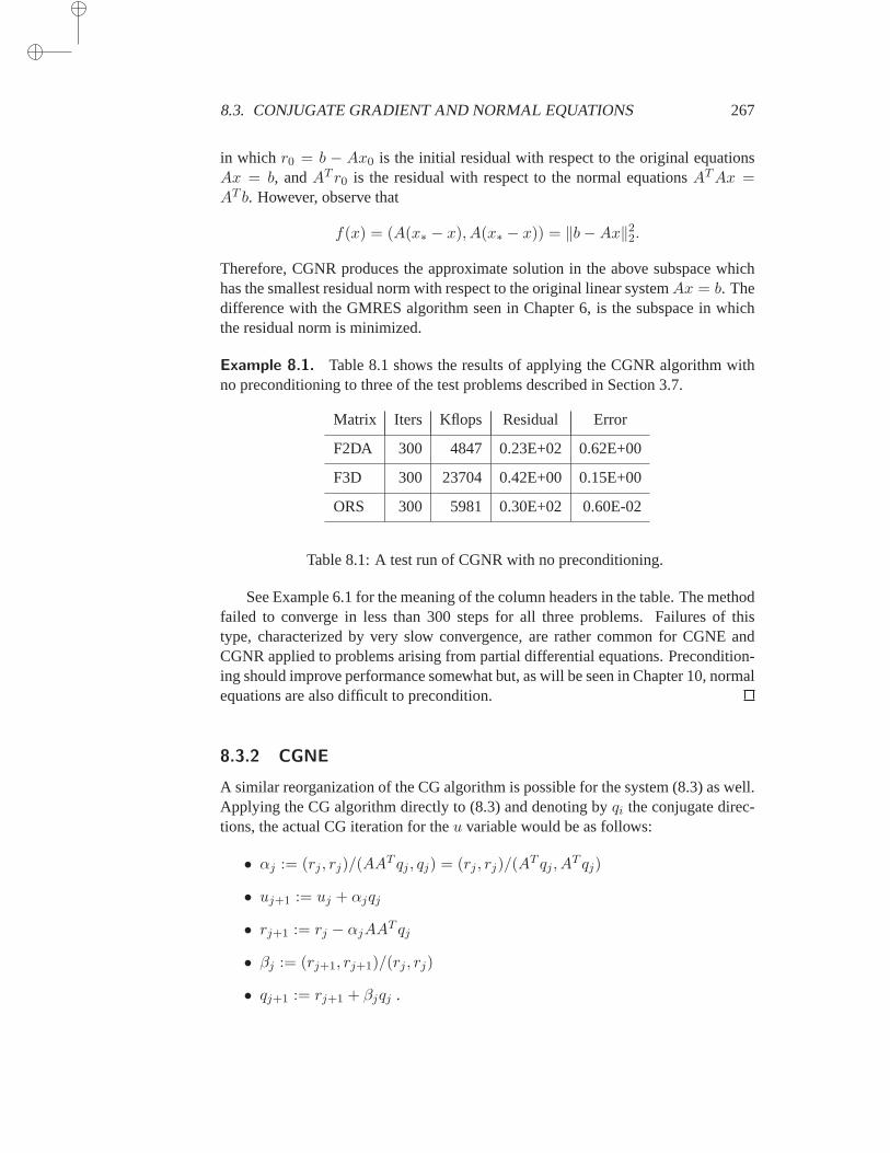
8.3. CONJUGATE GRADIENT AND NORMAL EQUATIONS 267
in which r0 = b − Ax0 is the initial residual with respect to the original equationsAx = b, andAT r0 is the residual with respect to the normal equationsATAx =AT b. However, observe that
f(x) = (A(x∗ − x), A(x∗ − x)) = ‖b−Ax‖22.
Therefore, CGNR produces the approximate solution in the above subspace whichhas the smallest residual norm with respect to the original linear systemAx = b. Thedifference with the GMRES algorithm seen in Chapter 6, is the subspace in whichthe residual norm is minimized.
Example 8.1. Table 8.1 shows the results of applying the CGNR algorithm withno preconditioning to three of the test problems described in Section 3.7.
Matrix Iters Kflops Residual Error
F2DA 300 4847 0.23E+02 0.62E+00
F3D 300 23704 0.42E+00 0.15E+00
ORS 300 5981 0.30E+02 0.60E-02
Table 8.1: A test run of CGNR with no preconditioning.
See Example 6.1 for the meaning of the column headers in the table. The methodfailed to converge in less than 300 steps for all three problems. Failures ofthistype, characterized by very slow convergence, are rather common forCGNE andCGNR applied to problems arising from partial differential equations. Precondition-ing should improve performance somewhat but, as will be seen in Chapter 10, normalequations are also difficult to precondition.
8.3.2 CGNE
A similar reorganization of the CG algorithm is possible for the system (8.3) as well.Applying the CG algorithm directly to (8.3) and denoting byqi the conjugate direc-tions, the actual CG iteration for theu variable would be as follows:
• αj := (rj , rj)/(AAT qj , qj) = (rj , rj)/(A
T qj , AT qj)
• uj+1 := uj + αjqj
• rj+1 := rj − αjAAT qj
• βj := (rj+1, rj+1)/(rj , rj)
• qj+1 := rj+1 + βjqj .
268 CHAPTER 8. METHODS RELATED TO THE NORMAL EQUATIONS
Notice that an iteration can be written with the original variablexi = x0 +AT (ui −u0) by introducing the vectorpi = AT qi. Then, the residual vectors for the vectorsxi andui are the same. No longer are theqi vectors needed because thepi’s canbe obtained aspj+1 := AT rj+1 + βjpj . The resulting algorithm described below,the Conjugate Gradient for the normal equations (CGNE), is also known asCraig’smethod.
ALGORITHM 8.5 CGNE (Craig’s Method)
1. Computer0 = b−Ax0, p0 = AT r0.2. Fori = 0, 1, . . . , until convergence Do:3. αi = (ri, ri)/(pi, pi)4. xi+1 = xi + αipi
5. ri+1 = ri − αiApi
6. βi = (ri+1, ri+1)/(ri, ri)7. pi+1 = AT ri+1 + βipi
8. EndDo
We now explore the optimality properties of this algorithm, as was done forCGNR. The approximationum related to the variablexm by xm = ATum is theactualm-th CG approximation for the linear system (8.3). Therefore, it minimizesthe energy norm of the error on the Krylov subspaceKm. In this case,um minimizesthe function
f(u) ≡ (AAT (u∗ − u), (u∗ − u))over all vectorsu in the affine Krylov subspace,
u0 +Km(AAT , r0) = u0 + spanr0, AAT r0, . . . , (AAT )m−1r0.
Notice thatr0 = b−AATu0 = b−Ax0. Also, observe that
f(u) = (AT (u∗ − u), AT (u∗ − u)) = ‖x∗ − x‖22,
wherex = ATu. Therefore, CGNE produces the approximate solution in the sub-space
x0 +ATKm(AAT , r0) = x0 +Km(ATA,AT r0)
which has the smallest 2-norm of the error. In addition, note that the subspacex0 +Km(ATA,AT r0) is identical with the subspace found for CGNR. Therefore,thetwo methods find approximations from the same subspace which achieve differentoptimality properties: minimal residual for CGNR and minimal error for CGNE.
8.4 Saddle-Point Problems
Now consider the equivalent system(
I AAT O
)(rx
)
=
(b0
)
8.4. SADDLE-POINT PROBLEMS 269
with r = b−Ax. This system can be derived from the necessary conditions appliedto the constrained least-squares problem (8.6–8.7). Thus, the 2-norm of b− r = Axis minimized implicitly under the constraintAT r = 0. Note thatA does not have tobe a square matrix.
This can be extended into a more general constrained quadratic optimizationproblem as follows:
minimizef(x) ≡ 1
2(Ax, x)− (x, b) (8.28)
subject toBTx = c. (8.29)
The necessary conditions for optimality yield the linear system(A BBT O
)(xy
)
=
(bc
)
(8.30)
in which the names of the variablesr, x are changed intox, y for notational con-venience. It is assumed that the column dimension ofB does not exceed its rowdimension. The Lagrangian for the above optimization problem is
L(x, y) =1
2(Ax, x)− (x, b) + (y, (BTx− c))
and the solution of (8.30) is the saddle point of the above Lagrangian. Optimizationproblems of the form (8.28–8.29) and the corresponding linear systems (8.30) areimportant and arise in many applications. Because they are intimately related to thenormal equations, we discuss them briefly here.
In the context of fluid dynamics, a well known iteration technique for solvingthe linear system (8.30) is Uzawa’s method, which resembles a relaxed blockSORiteration.
ALGORITHM 8.6 Uzawa’s Method
1. Choosex0, y0
2. Fork = 0, 1, . . . , until convergence Do:3. xk+1 = A−1(b−Byk)4. yk+1 = yk + ω(BTxk+1 − c)5. EndDo
The algorithm requires the solution of the linear system
Axk+1 = b−Byk (8.31)
at each iteration. By substituting the result of line 3 into line 4, thexk iterates can beeliminated to obtain the following relation for theyk’s,
yk+1 = yk + ω(BTA−1(b−Byk)− c
)

270 CHAPTER 8. METHODS RELATED TO THE NORMAL EQUATIONS
which is nothing but a Richardson iteration for solving the linear system
BTA−1By = BTA−1b− c. (8.32)
Apart from a sign, this system is the reduced system resulting from eliminatingthex variable from (8.30). Convergence results can be derived from the analysis of theRichardson iteration.
Corollary 8.1 Let A be a Symmetric Positive Definite matrix andB a matrix offull rank. ThenS = BTA−1B is also Symmetric Positive Definite and Uzawa’salgorithm converges, if and only if
0 < ω <2
λmax(S). (8.33)
In addition, the optimal convergence parameterω is given by
ωopt =2
λmin(S) + λmax(S).
Proof. The proof of this result is straightforward and is based on the results seen inExample 4.1.
It is interesting to observe that whenc = 0 andA is Symmetric Positive Defi-nite, then the system (8.32) can be regarded as the normal equations for minimizingtheA−1-norm of b − By. Indeed, the optimality conditions are equivalent to theorthogonality conditions
(b−By,Bw)A−1 = 0, ∀ w,
which translate into the linear systemBTA−1By = BTA−1b. As a consequence,the problem will tend to be easier to solve if the columns ofB are almost orthogonalwith respect to theA−1 inner product. This is true when solving theStokes problemwhereB represents the discretization of the gradient operator whileBT discretizesthe divergence operator, andA is the discretization of a Laplacian. In this case, ifit were not for the boundary conditions, the matrixBTA−1B would be the identity.This feature can be exploited in developing preconditioners for solving problemsof the form (8.30). Another particular case is whenA is the identity matrix andc = 0. Then, the linear system (8.32) becomes the system of the normal equationsforminimizing the 2-norm ofb − By. These relations provide insight in understandingthat the block form (8.30) is actually a form of normal equations for solvingBy = bin the least-squares sense. However, a different inner product is used.
In Uzawa’s method, a linear system at each step must be solved, namely, thesys-tem (8.31). Solving this system is equivalent to finding the minimum of the quadraticfunction
minimize fk(x) ≡1
2(Ax, x)− (x, b−Byk). (8.34)
8.4. SADDLE-POINT PROBLEMS 271
Apart from constants,fk(x) is the Lagrangian evaluated at the previousy iterate.The solution of (8.31), or the equivalent optimization problem (8.34), is expensive.A common alternative replaces thex-variable update (8.31) by taking one step in thegradient direction for the quadratic function (8.34), usually with fixed step-lengthǫ.The gradient offk(x) at the current iterate isAxk − (b − Byk). This results in theArrow-Hurwicz Algorithm.
ALGORITHM 8.7 The Arrow-Hurwicz algorithm
1. Select an initial guessx0, y0 to the system (8.30)2. Fork = 0, 1, . . . , until convergence Do:3. Computexk+1 = xk + ǫ(b−Axk −Byk)4. Computeyk+1 = yk + ω(BTxk+1 − c)5. EndDo
The above algorithm is a block-iteration of the form(
I O−ωBT I
)(xk+1
yk+1
)
=
(I − ǫA −ǫBO I
)(xk
yk
)
+
(ǫb−ωc
)
.
Uzawa’s method, and many similar techniques for solving (8.30), are basedonsolving the reduced system (8.32). An important observation here is that the Schurcomplement matrixS ≡ BTA−1B need not be formed explicitly. This can be usefulif this reduced system is to be solved by an iterative method. The matrixA is typicallyfactored by a Cholesky-type factorization. The linear systems with the coefficientmatrix A can also be solved by a preconditioned Conjugate Gradient method. Ofcourse these systems must then be solved accurately.
Sometimes it is useful to “regularize” the least-squares problem (8.28) by solvingthe following problem in its place:
minimizef(x) ≡ 1
2(Ax, x)− (x, b) + ρ(Cy, y)
subject toBTx = c
in which ρ is a scalar parameter. For example,C can be the identity matrix or thematrix BTB. The matrix resulting from the Lagrange multipliers approach thenbecomes (
A BBT ρC
)
.
The new Schur complement matrix is
S = ρC −BTA−1B.
Example 8.2. In the case whereC = BTB, the above matrix takes the form
S = BT (ρI −A−1)B.
272 CHAPTER 8. METHODS RELATED TO THE NORMAL EQUATIONS
Assuming thatA is SPD,S is also positive definite when
ρ ≥ 1
λmin(A).
However, it is alsonegative definitefor
ρ ≤ 1
λmax(A),
a condition which may be easier to satisfy on practice.
PROBLEMS
P-8.1 Derive the linear system (8.5) by expressing the standard necessary conditions for theproblem (8.6–8.7).
P-8.2 It was stated in Section 8.2.2 that when‖AT ei‖2 = 1 for i = 1, . . . , n, the vectorddefined in Algorithm 8.3 is equal toωAT r.
a. What does this become in the general situation when‖AT ei‖2 6= 1?
b. Is Cimmino’s method still equivalent to a Richardson iteration?
c. Show convergence results similar to those of the scaled case.
P-8.3 In Section 8.2.2, Cimmino’s algorithm was derived based on the Normal Residualformulation, i.e., on (8.1). Derive an “NE” formulation, i.e., an algorithm based on Jacobi’smethod for (8.3).
P-8.4 What are the eigenvalues of the matrix (8.5)? Derive a system whose coefficientmatrix has the form
B(α) =
(2αI AAT O
)
.
and which is also equivalent to the original systemAx = b. What are the eigenvalues ofB(α)? Plot the spectral norm ofB(α) as a function ofα.
P-8.5 It was argued in Section 8.4 that whenc = 0 the system (8.32) is nothing but thenormal equations for minimizing theA−1-norm of the residualr = b−By.
a. Write the associated CGNR approach for solving this problem. Find a variant thatrequires only one linear system solution with the matrixA at each CG step [Hint:Write the CG algorithm for the associated normal equations and see how the resultingprocedure can be reorganized to save operations]. Find alsoa variant that is suitablefor the case where the Cholesky factorization ofA is available.
b. Derive a method for solving the equivalent system (8.30) for the case whenc = 0 andthen for the general case wjenc 6= 0. How does this technique compare with Uzawa’smethod?
P-8.6 Consider the linear system (8.30) in whichc = 0 andB is of full rank. Define thematrix
P = I −B(BTB)−1BT .
8.4. SADDLE-POINT PROBLEMS 273
a. Show thatP is a projector. Is it an orthogonal projector? What are the range and nullspaces ofP?
b. Show that the unknownx can be found by solving the linear system
PAPx = Pb, (8.35)
in which the coefficient matrix is singular but the system is consistent, i.e., there is anontrivial solution because the right-hand side is in the range of the matrix (see Chapter1).
c. What must be done toadapt the Conjugate Gradient Algorithmfor solving the abovelinear system (which is symmetric, but not positive definite)? In which subspace arethe iterates generated from the CG algorithm applied to (8.35)?
d. Assume that the QR factorization of the matrixB is computed. Write an algorithmbased on the approach of the previous questions for solving the linear system (8.30).
P-8.7 Show that Uzawa’s iteration can be formulated as a fixed-point iteration associatedwith the splittingC = M −N with
M =
(A O
−ωBT I
)
, N =
(O −BO I
)
.
Derive the convergence result of Corollary 8.1 .
P-8.8 Show that each new vector iterate in Cimmino’s method is suchthat
xnew = x+ ωA−1∑
i
Pir,
wherePi is defined by (8.24).
P-8.9 In Uzawa’s method a linear system with the matrixA must be solved at each step.Assume that these systems are solved inaccurately by an iterative process. For each linearsystem the iterative process is applied until the norm of theresidualrk+1 = (b − Byk) −Axk+1 is less than a certain thresholdǫk+1.
a. Assume thatω is chosen so that (8.33) is satisfied and thatǫk converges to zero asktends to infinity. Show that the resulting algorithm converges to the solution.
b. Give an explicit upper bound of the error onyk in the case whenǫi is chosen of theform ǫ = αi, whereα < 1.
P-8.10 Assume‖b − Ax‖2 is to be minimized, in whichA is n ×m with n > m. Let x∗be the minimizer andr = b−Ax∗. What is the minimizer of‖(b+ αr)−Ax‖2, whereα isan arbitrary scalar?
P-8.11
P-8.12 Consider a saddle-point linear system of the formAx = b, where
A =
(B CCT 0
)
; x =
(up
)
; b =
(f0
)
in which B is symmetric positive definite. It is assumed thatA is nonsingular (which isequivalent to assuming thatC is of full rank).
1. Prove thatA has both negative and positive eigenvalues by showing how toselectvectorsx =
(up
)
so that(Ax, x) > 0 and vectorsx so that(Ax, x) < 0.
274 CHAPTER 8. METHODS RELATED TO THE NORMAL EQUATIONS
2. Show how to select an initial guess of the formx0 =(
u0
0
)if we want its corresponding
residual vectorr0 = b−Ax0 to be of the formr0 =(
0s0
)
. What happens if we attemptto use the steepest descent algorithm with this initial guess?
3. What happens if the Minimal Residual iteration is applied using the same initial guessas in the previous question?
4. By eliminating the unknownu find a linear systemSp = g that must be satisfied bythe variablep Is the coefficient matrix of this system Symmetric Positive Definite (orSymmetric Negative Definite)?
5. We now want to solve the linear system by the following iteration:
uk+1 = B−1(f − Cpk)
pk+1 = pk + αkCTuk+1
Show thatpk+1 is of the formpk+1 = pk + αksk wheresk is the residual relativeto pk for the reduced linear system found in the previous question. How shouldαk
be selected if we wantpk+1 to correspond to the iterate of steepest descent for thisreduced system.
NOTES AND REFERENCES. Methods based on the normal equations have been among the first tobe used for solving nonsymmetric linear systems by iterative methods [181, 85]. The work by Bjorkand Elfing [39], and Sameh et al. [182, 53, 52] revived these techniques by showing that they havesome advantages from the implementation point of view, and that they can offer good performance fora broad class of problems. In addition, they are also attractive for parallel computers. In [240], a fewpreconditioning ideas for normal equations were described and these will be covered in Chapter 10. Itwould be helpful to be able to determine whether or not it is preferable to use the normal equations ap-proach rather than the “direct equations” for a given system, but this may require an eigenvalue/singularvalue analysis.
It is sometimes argued that the normal equations approach isalwaysbetter than the standardapproach, because it has a quality of robustness which outweighs the additional cost due to the slownessof the method in the generic elliptic case. Unfortunately, this is not true. Although variants of theKaczmarz and Cimmino algorithms deserve a place in any robust iterativesolution package, they cannotbe viewed as a panacea. Inmost realistic examples arising from Partial Differential Equations, thenormal equations route gives rise to much slower convergence than theKrylov subspace approach forthe direct equations. For ill-conditioned problems, these methods will simplyfail to converge, unless agood preconditioner is available.
Chapter 9
PRECONDITIONED ITERATIONS
Although the methods seen in previous chapters are well founded theoretically, they are all likely
to suffer from slow convergence for problems which arise from typical applications such as fluid
dynamics or electronic device simulation. Preconditioning is a key ingredient for the success
of Krylov subspace methods in these applications. This chapter discusses the preconditioned
versions of the iterative methods already seen, but without being specific about the particu-
lar preconditioners used. The standard preconditioning techniques will be covered in the next
chapter.
9.1 Introduction
Lack of robustness is a widely recognized weakness of iterative solvers, relative todirect solvers. This drawback hampers the acceptance of iterative methods in indus-trial applications despite their intrinsic appeal for very large linear systems.Boththe efficiency and robustness of iterative techniques can be improved byusingpre-conditioning. A term introduced in Chapter 4, preconditioning is simply a meansof transforming the original linear system into one which has the same solution,butwhich is likely to be easier to solve with an iterative solver. In general, the relia-bility of iterative techniques, when dealing with various applications, depends muchmore on the quality of the preconditioner than on the particular Krylov subspace ac-celerators used. We will cover some of these preconditioners in detail in the nextchapter. This chapter discusses the preconditioned versions of the Krylov subspacealgorithms already seen, using a generic preconditioner.
To begin with, it is worthwhile to consider the options available for precondi-tioning a system. The first step in preconditioning is to find a preconditioning matrixM . The matrixM can be defined in many different ways but it must satisfy a fewminimal requirements. From a practical point of view, the most requirement forM isthat it is inexpensive to solve linear systemsMx = b. This is because the precondi-tioned algorithms will all require a linear system solution with the matrixM at eachstep. AlsoM should close toA in some sense and it should clearly be nonsingular.Chapter 10 explores in detail the problem of finding preconditionersM for a givenmatrixS, while this chapter considers only the ways in which the preconditioner isapplied to solve the original system.
Once a preconditioning matrixM is available there are three known ways of ap-
275
276 CHAPTER 9. PRECONDITIONED ITERATIONS
plying the preconditioner. The precondiotioner can be applied from the left, leadingto the preconditioned system
M−1Ax = M−1b (9.1)
Alternatively, it can also be applied to the right:
AM−1u = b, x ≡M−1u . (9.2)
Note that the above formulation amounts to making the change of variablesu = Mx,and solving the system with respect to the unknownu. Finally, a common situationis when the preconditioner is available in the factored form
M = MLMR
where, typicallyML andMR are triangular matrices. In this situation, the precondi-tioning can be split:
M−1L AM−1
R u = M−1L b, x ≡M−1
R u . (9.3)
It is imperative to preserve symmetry when the original matrix is symmetric, so thesplit preconditioner seems mandatory this case. However, there are otherways of pre-serving symmetry, or rather to take advantage of symmetry, even ifM is not availablein a factored form. This is discussed next for the Conjugate Gradient method.
9.2 Preconditioned Conjugate Gradient
Consider a matrixA that is symmetric and positive definite and assume that a pre-conditionerM is available. The preconditionerM is a matrix which approximatesA in some yet-undefined sense. It is assumed thatM is also Symmetric PositiveDefinite. Then, one can precondition the system in the three ways shown in the pre-vious section, i.e., as in (9.1), (9.2), or (9.3). Note that the first two systemsare nolonger symmetric in general. The next section considers strategies for preservingsymmetry. Then, efficient implementations will be described for particular forms ofthe preconditioners.
9.2.1 Preserving Symmetry
WhenM is available in the form of an incomplete Cholesky factorization, i.e., when
M = LLT ,
then a simple way to preserve symmetry is to use the “split” the preconditioningoption (9.3) which yields the Symmetric Positive Definite matrix,
L−1AL−Tu = L−1b, x = L−Tu. (9.4)
9.2. PRECONDITIONED CONJUGATE GRADIENT 277
However, it is not necessary to split the preconditioner in this manner in order topreserve symmetry. Observe thatM−1A is self-adjoint for theM -inner product,
(x, y)M ≡ (Mx, y) = (x,My)
since
(M−1Ax, y)M = (Ax, y) = (x,Ay) = (x,M(M−1A)y) = (x,M−1Ay)M .
Therefore, an alternative is to replace the usual Euclidean inner product in the Con-jugate Gradient algorithm by theM -inner product.
If the CG algorithm is rewritten for this new inner product, denoting byrj =b−Axj the original residual and byzj = M−1rj the residual for the preconditionedsystem, the following sequence of operations is obtained, ignoring the initial step:
1. αj := (zj , zj)M/(M−1Apj , pj)M
2. xj+1 := xj + αjpj
3. rj+1 := rj − αjApj andzj+1 := M−1rj+1
4. βj := (zj+1, zj+1)M/(zj , zj)M
5. pj+1 := zj+1 + βjpj
Since(zj , zj)M = (rj , zj) and(M−1Apj , pj)M = (Apj , pj), theM -inner productsdo not have to be computed explicitly. With this observation, the following algorithmis obtained.
ALGORITHM 9.1 Preconditioned Conjugate Gradient
1. Computer0 := b−Ax0, z0 = M−1r0, andp0 := z02. Forj = 0, 1, . . ., until convergence Do:3. αj := (rj , zj)/(Apj , pj)4. xj+1 := xj + αjpj
5. rj+1 := rj − αjApj
6. zj+1 := M−1rj+1
7. βj := (rj+1, zj+1)/(rj , zj)8. pj+1 := zj+1 + βjpj
9. EndDo
It is interesting to observe thatM−1A is also self-adjoint with respect to theAinner-product. Indeed,
(M−1Ax, y)A = (AM−1Ax, y) = (x,AM−1Ay) = (x,M−1Ay)A
and a similar algorithm can be written for this dot product (see Exercise 2).In the case whereM is a Cholesky productM = LLT , two options are available,
namely, the split preconditioning option (9.4), or the above algorithm. An immediate
278 CHAPTER 9. PRECONDITIONED ITERATIONS
question arises about the iterates produced by these two options: Is one better thanthe other? Surprisingly, the answer is thatthe iterates are identical. To see this, startfrom Algorithm 9.1 and define the following auxiliary vectors and matrix from it:
pj = LT pj
uj = LTxj
rj = LT zj = L−1rj
A = L−1AL−T .
Observe that
(rj , zj) = (rj , L−TL−1rj) = (L−1rj , L
−1rj) = (rj , rj).
Similarly,
(Apj , pj) = (AL−T pj , L−T pj)(L
−1AL−T pj , pj) = (Apj , pj).
All the steps of the algorithm can be rewritten with the new variables, yielding thefollowing sequence of operations:
1. αj := (rj , rj)/(Apj , pj)
2. uj+1 := uj + αj pj
3. rj+1 := rj − αjApj
4. βj := (rj+1, rj+1)/(rj , rj)
5. pj+1 := rj+1 + βj pj .
This is precisely the Conjugate Gradient algorithm applied to the preconditionedsystem
Au = L−1b
whereu = LTx. It is common when implementing algorithms which involve a rightpreconditioner to avoid the use of theu variable, since the iteration can be writtenwith the originalx variable. If the above steps are rewritten with the originalx andpvariables, the following algorithm results.
ALGORITHM 9.2 Split Preconditioner Conjugate Gradient
1. Computer0 := b−Ax0; r0 = L−1r0; andp0 := L−T r0.2. Forj = 0, 1, . . ., until convergence Do:3. αj := (rj , rj)/(Apj , pj)4. xj+1 := xj + αjpj
5. rj+1 := rj − αjL−1Apj
6. βj := (rj+1, rj+1)/(rj , rj)7. pj+1 := L−T rj+1 + βjpj
8. EndDo
9.2. PRECONDITIONED CONJUGATE GRADIENT 279
The iteratesxj produced by the above algorithm and Algorithm 9.1 are identical,provided the same initial guess is used.
Consider now the right preconditioned system (9.2). The matrixAM−1 is notHermitian with either the Standard inner product or theM -inner product. However,it is Hermitian with respect to theM−1-inner product. If the CG-algorithm is writtenwith respect to theu-variable and for this new inner product, the following sequenceof operations would be obtained, ignoring again the initial step:
1. αj := (rj , rj)M−1/(AM−1pj , pj)M−1
2. uj+1 := uj + αjpj
3. rj+1 := rj − αjAM−1pj
4. βj := (rj+1, rj+1)M−1/(rj , rj)M−1
5. pj+1 := rj+1 + βjpj .
Recall that theu vectors and thex vectors are related byx = M−1u. Since theu vectors are not actually needed, the update foruj+1 in the second step can bereplaced byxj+1 := xj + αjM
−1pj . Then observe that the whole algorithm can berecast in terms ofqj = M−1pj andzj = M−1rj .
1. αj := (zj , rj)/(Aqj , qj)
2. xj+1 := xj + αjqj
3. rj+1 := rj − αjAqj andzj+1 = M−1rj+1
4. βj := (zj+1, rj+1)/(zj , rj)
5. qj+1 := zj+1 + βjqj .
Notice that the same sequence of computations is obtained as with Algorithm9.1, the left preconditioned Conjugate Gradient. The implication is thatthe left pre-conditioned CG algorithm with theM -inner product is mathematically equivalent tothe right preconditioned CG algorithm with theM−1-inner product.
9.2.2 Efficient Implementations
When applying a Krylov subspace procedure to a preconditioned linear system, anoperation of the form
v → w = M−1Av
or some similar operation is performed at each step. The most natural way to performthis operation is to multiply the vectorv by A and then applyM−1 to the result.However, sinceA andM are related, it is sometimes possible to devise proceduresthat are more economical than this straightforward approach. For example, it is oftenthe case that
M = A−R
280 CHAPTER 9. PRECONDITIONED ITERATIONS
in which the number of nonzero elements inR is much smaller than inA. In thiscase, the simplest scheme would be to computew = M−1Av as
w = M−1Av = M−1(M +R)v = v +M−1Rv.
This requires thatR be stored explicitly. In approximateLU factorization tech-niques,R is the matrix of the elements that are dropped during the incomplete fac-torization. An even more efficient variation of the preconditioned ConjugateGradientalgorithm can be derived for some common forms of the preconditioner in the specialsituation whereA is symmetric. WriteA in the form
A = D0 − E − ET (9.5)
in which−E is the strict lower triangular part ofA andD0 its diagonal. In manycases, the preconditionerM can be written in the form
M = (D − E)D−1(D − ET ) (9.6)
in whichE is the same as above andD is some diagonal, not necessarily equal toD0.For example, in the SSOR preconditioner withω = 1, D ≡ D0. Also, for certaintypes of matrices, the IC(0) preconditioner can be expressed in this manner, whereD can be obtained by a recurrence formula.
Eisenstat’s implementationconsists of applying the Conjugate Gradient algo-rithm to the linear system
Au = (D − E)−1b (9.7)
withA ≡ (D − E)−1A(D − ET )−1, x = (D − ET )−1u. (9.8)
This does not quite correspond to a preconditioning with the matrix (9.6). In orderto produce the same iterates as Algorithm 9.1, the matrixA must be further pre-conditioned with the diagonal matrixD−1. Thus, the preconditioned CG algorithm,Algorithm 9.1, is actually applied to the system (9.7) in which the preconditioningoperation isM−1 = D. Alternatively, we can initially scale the rows and columns ofthe linear system and preconditioning to transform the diagonal to the identity.SeeExercise 7.
Now note that
A = (D − E)−1A(D − ET )−1
= (D − E)−1(D0 − E − ET )(D − ET )−1
= (D − E)−1(D0 − 2D + (D − E) + (D − ET )
)(D − ET )−1
≡ (D − E)−1D1(D − ET )−1 + (D − E)−1 + (D − ET )−1,
in whichD1 ≡ D0 − 2D. As a result,
Av = (D − E)−1[v +D1(D − ET )−1v
]+ (D − ET )−1v.
Thus, the vectorw = Av can be computed by the following procedure:
9.2. PRECONDITIONED CONJUGATE GRADIENT 281
z := (D − ET )−1vw := (D − E)−1(v +D1z)w := w + z.
One product with the diagonalD can be saved if the matricesD−1E andD−1ET
are stored. Indeed, by settingD1 = D−1D1 and v = D−1v, the above procedurecan be reformulated as follows.
ALGORITHM 9.3 Computation ofw = Av
1. v := D−1v2. z := (I −D−1ET )−1v
3. w := (I −D−1E)−1(v + D1z)4. w := w + z .
Note that the matricesD−1E andD−1ET are not the transpose of one another, sowe actually need to increase the storage requirement for this formulation if thesematrices are stored. However, there is a more economical variant which works withthe matrixD−1/2ED−1/2 and its transpose. This is left as Exercise 8.
Denoting byNz(X) the number of nonzero elements of a sparse matrixX, thetotal number of operations (additions and multiplications) of this procedure isn for(1), 2Nz(E
T ) for (2), 2Nz(E) + 2n for (3), andn for (4). The cost of the precondi-tioning operation byD−1, i.e.,n operations, must be added to this, yielding the totalnumber of operations:
Nop = n+ 2Nz(E) + 2Nz(ET ) + 2n+ n+ n
= 3n+ 2(Nz(E) +Nz(ET ) + n)
= 3n+ 2Nz(A).
For the straightforward approach,2Nz(A) operations are needed for the product withA, 2Nz(E) for the forward solve, andn + 2Nz(E
T ) for the backward solve givinga total of
2Nz(A) + 2Nz(E) + n+ 2Nz(ET ) = 4Nz(A)− n.
Thus, Eisenstat’s scheme is always more economical, whenNz is large enough, al-though the relative gains depend on the total number of nonzero elements inA. Onedisadvantage of this scheme is that it is limited to a special form of the preconditioner.
Example 9.1. For a 5-point finite difference matrix,Nz(A) is roughly5n, so thatwith the standard implementation19n operations are performed, while with Eisen-stat’s implementation only13n operations would be performed, a savings of about1
3 .However, if the other operations of the Conjugate Gradient algorithm are included,for a total of about10n operations, the relative savings become smaller. Now theoriginal scheme will require29n operations, versus23n operations for Eisenstat’simplementation.
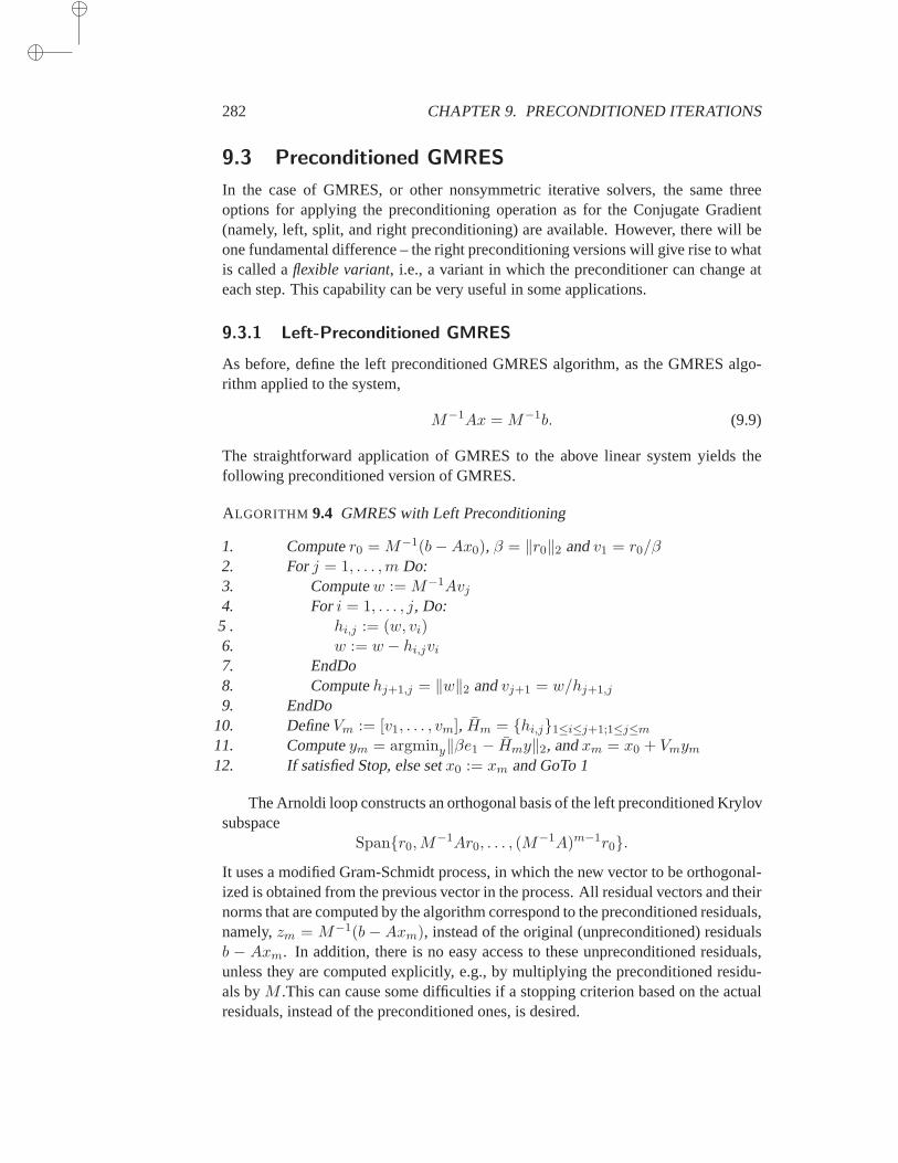
282 CHAPTER 9. PRECONDITIONED ITERATIONS
9.3 Preconditioned GMRES
In the case of GMRES, or other nonsymmetric iterative solvers, the same threeoptions for applying the preconditioning operation as for the Conjugate Gradient(namely, left, split, and right preconditioning) are available. However, there will beone fundamental difference – the right preconditioning versions will give rise to whatis called aflexible variant, i.e., a variant in which the preconditioner can change ateach step. This capability can be very useful in some applications.
9.3.1 Left-Preconditioned GMRES
As before, define the left preconditioned GMRES algorithm, as the GMRES algo-rithm applied to the system,
M−1Ax = M−1b. (9.9)
The straightforward application of GMRES to the above linear system yields thefollowing preconditioned version of GMRES.
ALGORITHM 9.4 GMRES with Left Preconditioning
1. Computer0 = M−1(b−Ax0), β = ‖r0‖2 andv1 = r0/β2. Forj = 1, . . . ,m Do:3. Computew := M−1Avj
4. Fori = 1, . . . , j, Do:5 . hi,j := (w, vi)6. w := w − hi,jvi
7. EndDo8. Computehj+1,j = ‖w‖2 andvj+1 = w/hj+1,j
9. EndDo10. DefineVm := [v1, . . . , vm], Hm = hi,j1≤i≤j+1;1≤j≤m
11. Computeym = argminy‖βe1 − Hmy‖2, andxm = x0 + Vmym
12. If satisfied Stop, else setx0 := xm and GoTo 1
The Arnoldi loop constructs an orthogonal basis of the left preconditioned Krylovsubspace
Spanr0,M−1Ar0, . . . , (M−1A)m−1r0.
It uses a modified Gram-Schmidt process, in which the new vector to be orthogonal-ized is obtained from the previous vector in the process. All residual vectors and theirnorms that are computed by the algorithm correspond to the preconditioned residuals,namely,zm = M−1(b − Axm), instead of the original (unpreconditioned) residualsb − Axm. In addition, there is no easy access to these unpreconditioned residuals,unless they are computed explicitly, e.g., by multiplying the preconditioned residu-als byM .This can cause some difficulties if a stopping criterion based on the actualresiduals, instead of the preconditioned ones, is desired.
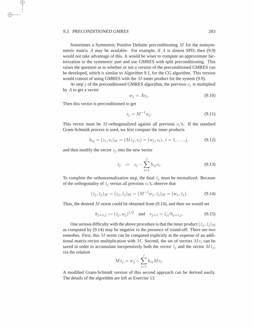
9.3. PRECONDITIONED GMRES 283
Sometimes a Symmetric Positive Definite preconditioningM for the nonsym-metric matrixA may be available. For example, ifA is almost SPD, then (9.9)would not take advantage of this. It would be wiser to compute an approximatefac-torization to the symmetric part and use GMRES with split preconditioning. Thisraises the question as to whether or not a version of the preconditioned GMRES canbe developed, which is similar to Algorithm 9.1, for the CG algorithm. This versionwould consist of using GMRES with theM -inner product for the system (9.9).
At stepj of the preconditioned GMRES algorithm, the previousvj is multipliedbyA to get a vector
wj = Avj . (9.10)
Then this vector is preconditioned to get
zj = M−1wj . (9.11)
This vector must beM -orthogonalized against all previousvi’s. If the standardGram-Schmidt process is used, we first compute the inner products
hij = (zj , vi)M = (Mzj , vi) = (wj , vi), i = 1, . . . , j, (9.12)
and then modify the vectorzj into the new vector
zj := zj −j∑
i=1
hijvi. (9.13)
To complete the orthonormalization step, the finalzj must be normalized. Becauseof the orthogonality ofzj versus all previousvi’s, observe that
(zj , zj)M = (zj , zj)M = (M−1wj , zj)M = (wj , zj). (9.14)
Thus, the desiredM -norm could be obtained from (9.14), and then we would set
hj+1,j := (zj , wj)1/2 and vj+1 = zj/hj+1,j . (9.15)
One serious difficulty with the above procedure is that the inner product(zj , zj)M
as computed by (9.14) may be negative in the presence of round-off. There are tworemedies. First, thisM -norm can be computed explicitly at the expense of an addi-tional matrix-vector multiplication withM . Second, the set of vectorsMvi can besaved in order to accumulate inexpensively both the vectorzj and the vectorMzj ,via the relation
Mzj = wj −j∑
i=1
hijMvi.
A modified Gram-Schmidt version of this second approach can be derivedeasily.The details of the algorithm are left as Exercise 13.
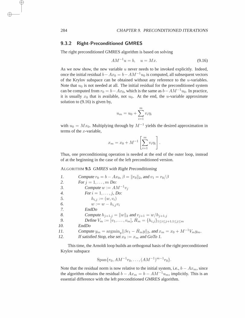
284 CHAPTER 9. PRECONDITIONED ITERATIONS
9.3.2 Right-Preconditioned GMRES
The right preconditioned GMRES algorithm is based on solving
AM−1u = b, u = Mx. (9.16)
As we now show, the new variableu never needs to be invoked explicitly. Indeed,once the initial residualb−Ax0 = b−AM−1u0 is computed, all subsequent vectorsof the Krylov subspace can be obtained without any reference to theu-variables.Note thatu0 is not needed at all. The initial residual for the preconditioned systemcan be computed fromr0 = b−Ax0, which is the same asb−AM−1u0. In practice,it is usuallyx0 that is available, notu0. At the end, theu-variable approximatesolution to (9.16) is given by,
um = u0 +
m∑
i=1
viηi
with u0 = Mx0. Multiplying through byM−1 yields the desired approximation interms of thex-variable,
xm = x0 +M−1
[m∑
i=1
viηi
]
.
Thus, one preconditioning operation is needed at the end of the outer loop, insteadof at the beginning in the case of the left preconditioned version.
ALGORITHM 9.5 GMRES with Right Preconditioning
1. Computer0 = b−Ax0, β = ‖r0‖2, andv1 = r0/β2. Forj = 1, . . . ,m Do:3. Computew := AM−1vj
4. Fori = 1, . . . , j, Do:5. hi,j := (w, vi)6. w := w − hi,jvi
7. EndDo8. Computehj+1,j = ‖w‖2 andvj+1 = w/hj+1,j
9. DefineVm := [v1, . . . , vm], Hm = hi,j1≤i≤j+1;1≤j≤m
10. EndDo11. Computeym = argminy‖βe1 − Hmy‖2, andxm = x0 +M−1Vmym.12. If satisfied Stop, else setx0 := xm and GoTo 1.
This time, the Arnoldi loop builds an orthogonal basis of the right preconditionedKrylov subspace
Spanr0, AM−1r0, . . . , (AM−1)m−1r0.
Note that the residual norm is now relative to the initial system, i.e.,b−Axm, sincethe algorithm obtains the residualb − Axm = b − AM−1um, implicitly. This is anessential difference with the left preconditioned GMRES algorithm.
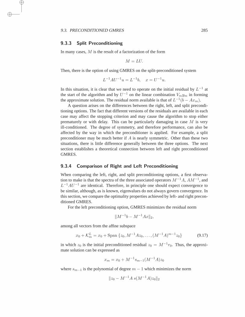
9.3. PRECONDITIONED GMRES 285
9.3.3 Split Preconditioning
In many cases,M is the result of a factorization of the form
M = LU.
Then, there is the option of using GMRES on the split-preconditioned system
L−1AU−1u = L−1b, x = U−1u.
In this situation, it is clear that we need to operate on the initial residual byL−1 atthe start of the algorithm and byU−1 on the linear combinationVmym in formingthe approximate solution. The residual norm available is that ofL−1(b−Axm).
A question arises on the differences between the right, left, and split precondi-tioning options. The fact that different versions of the residuals are available in eachcase may affect the stopping criterion and may cause the algorithm to stop eitherprematurely or with delay. This can be particularly damaging in caseM is veryill-conditioned. The degree of symmetry, and therefore performance, can also beaffected by the way in which the preconditioner is applied. For example, a splitpreconditioner may be much better ifA is nearly symmetric. Other than these twosituations, there is little difference generally between the three options. The nextsection establishes a theoretical connection between left and right preconditionedGMRES.
9.3.4 Comparison of Right and Left Preconditioning
When comparing the left, right, and split preconditioning options, a first observa-tion to make is that the spectra of the three associated operatorsM−1A,AM−1, andL−1AU−1 are identical. Therefore, in principle one should expect convergencetobe similar, although, as is known, eigenvalues do not always govern convergence. Inthis section, we compare the optimality properties achieved by left- and right precon-ditioned GMRES.
For the left preconditioning option, GMRES minimizes the residual norm
‖M−1b−M−1Ax‖2,
among all vectors from the affine subspace
x0 +KLm = x0 + Span z0,M−1Az0, . . . , (M
−1A)m−1z0 (9.17)
in which z0 is the initial preconditioned residualz0 = M−1r0. Thus, the approxi-mate solution can be expressed as
xm = x0 +M−1sm−1(M−1A)z0
wheresm−1 is the polynomial of degreem− 1 which minimizes the norm
‖z0 −M−1A s(M−1A)z0‖2
286 CHAPTER 9. PRECONDITIONED ITERATIONS
among all polynomialss of degree≤ m − 1. It is also possible to express thisoptimality condition with respect to the original residual vectorr0. Indeed,
z0 −M−1A s(M−1A)z0 = M−1[r0 −A s(M−1A)M−1r0
].
A simple algebraic manipulation shows that for any polynomials,
s(M−1A)M−1r = M−1s(AM−1)r, (9.18)
from which we obtain the relation
z0 −M−1As(M−1A)z0 = M−1[r0 −AM−1s(AM−1)r0
]. (9.19)
Consider now the situation with the right preconditioned GMRES. Here, it isnecessary to distinguish between the originalx variable and the transformed variableu related tox by x = M−1u. For theu variable, the right preconditioned GMRESprocess minimizes the 2-norm ofr = b−AM−1u whereu belongs to
u0 +KRm = u0 + Span r0, AM−1r0, . . . , (AM
−1)m−1r0 (9.20)
in whichr0 is the residualr0 = b−AM−1u0. This residual is identical to the resid-ual associated with the originalx variable sinceM−1u0 = x0. Multiplying (9.20)through to the left byM−1 and exploiting again (9.18), observe that the generic vari-ablex associated with a vector of the subspace (9.20) belongs to the affine subspace
M−1u0 +M−1KRm = x0 + Span z0,M−1Az0 . . . , (M
−1A)m−1z0.This is identical to the affine subspace (9.17) invoked in the left preconditioned vari-ant. In other words, for the right preconditioned GMRES, the approximatex-solutioncan also be expressed as
xm = x0 + sm−1(AM−1)r0.
However, nowsm−1 is a polynomial of degreem− 1 which minimizes the norm
‖r0 −AM−1 s(AM−1)r0‖2 (9.21)
among all polynomialss of degree≤ m − 1. What is surprising is that the twoquantities which are minimized, namely, (9.19) and (9.21), differ only by a multi-plication byM−1. Specifically, the left preconditioned GMRES minimizesM−1r,whereas the right preconditioned variant minimizesr, wherer is taken over the samesubspace in both cases.
Proposition 9.1 The approximate solution obtained by left or right preconditionedGMRES is of the form
xm = x0 + sm−1(M−1A)z0 = x0 +M−1sm−1(AM
−1)r0
wherez0 = M−1r0 and sm−1 is a polynomial of degreem − 1. The polynomialsm−1 minimizes the residual norm‖b − Axm‖2 in the right preconditioning case,and the preconditioned residual norm‖M−1(b−Axm)‖2 in the left preconditioningcase.
9.4. FLEXIBLE VARIANTS 287
In most practical situations, the difference in the convergence behaviorof thetwo approaches is not significant. The only exception is whenM is ill-conditionedwhich could lead to substantial differences.
9.4 Flexible Variants
In the discussion of preconditioning techniques so far, it is implicitly assumed thatthe preconditioning matrixM is fixed, i.e., it does not change from step to step.However, in some cases, no matrixM is available. Instead, the operationM−1x isthe result of some unspecified computation, possibly another iterative process. Insuch cases, it may well happen thatM−1 is not a constant operator. The previouspreconditioned iterative procedures will not converge ifM is not constant. Thereare a number of variants of iterative procedures developed in the literature that canaccommodate variations in the preconditioner, i.e., that allow the preconditionertovary from step to step. Such iterative procedures are called “flexible” iterations. Oneof these iterations, a flexible variant of the GMRES algorithm, is described next.
9.4.1 Flexible GMRES
We begin by examining the right preconditioned GMRES algorithm. In line 11 ofAlgorithm 9.5 the approximate solutionxm is expressed as a linear combinationof the preconditioned vectorszi = M−1vi, i = 1, . . . ,m. These vectors are alsocomputed in line 3, prior to their multiplication byA to obtain the vectorw. Theyare all obtained by applying the same preconditioning matrixM−1 to thevi’s. As aresult it is not necessary to save them. Instead, we only need to applyM−1 to thelinear combination of thevi’s, i.e., toVmym in line 11.
Suppose now that the preconditioner could change at every step, i.e., that zj isgiven by
zj = M−1j vj .
Then it would be natural to compute the approximate solution as
xm = x0 + Zmym
in whichZm = [z1, . . . , zm], andym is computed as before, as the solution to theleast-squares problem in line 11. These are the only changes that lead from the rightpreconditioned algorithm to the flexible variant, described below.
ALGORITHM 9.6 Flexible GMRES (FGMRES)
1. Computer0 = b−Ax0, β = ‖r0‖2, andv1 = r0/β2. Forj = 1, . . . ,m Do:3. Computezj := M−1
j vj
4. Computew := Azj5. Fori = 1, . . . , j, Do:6. hi,j := (w, vi)7. w := w − hi,jvi
288 CHAPTER 9. PRECONDITIONED ITERATIONS
8. EndDo9. Computehj+1,j = ‖w‖2 andvj+1 = w/hj+1,j
10. DefineZm := [z1, . . . , zm], Hm = hi,j1≤i≤j+1;1≤j≤m
11. EndDo12. Computeym = argminy‖βe1 − Hmy‖2, andxm = x0 + Zmym.13. If satisfied Stop, else setx0 ← xm and GoTo 1.
As can be seen, the main difference with the right preconditioned version,Al-gorithm 9.5, is that the preconditioned vectorszj = M−1
j vj must be saved and thesolution updated using these vectors. It is clear that whenMj = M for j = 1, . . . ,m,then this method is equivalent mathematically to Algorithm 9.5. It is important to ob-serve thatzj can be defined in line 3 without reference to any preconditioner. Thatis, any given new vectorzj can be chosen. This added flexibility may cause the algo-rithm some problems. Indeed,zj may be so poorly selected that a breakdown couldoccur, as in the worst-case scenario whenzj is zero.
One difference between FGMRES and the usual GMRES algorithm is that theaction ofAM−1
j on a vectorv of the Krylov subspace is no longer in the span ofVm+1. Instead, it is easy to show that
AZm = Vm+1Hm (9.22)
in replacement of the simpler relation(AM−1)Vm = Vm+1 Hm which holds forthe standard preconditioned GMRES; see (6.7). As before,Hm denotes them ×mmatrix obtained fromHm by deleting its last row andvj+1 is the vectorw which isnormalized in line 9 of Algorithm 9.6 to obtainvj+1. Then, the following alternativeformulation of (9.22) is valid, even whenhm+1,m = 0:
AZm = VmHm + vm+1eTm. (9.23)
An optimality property similar to the one which defines GMRES can be proved.Consider the residual vector for an arbitrary vectorz = x0 +Zmy in the affine spacex0 + spanZm. This optimality property is based on the relations
b−Az = b−A(x0 + Zmy)
= r0 −AZmy (9.24)
= βv1 − Vm+1Hmy
= Vm+1[βe1 − Hmy]. (9.25)
If Jm(y) denotes the function
Jm(y) = ‖b−A[x0 + Zmy]‖2,observe that by (9.25) and the fact thatVm+1 is unitary,
Jm(y) = ‖βe1 − Hmy‖2. (9.26)
Since the algorithm minimizes this norm over all vectorsu in Rm to yield ym, it is
clear that the approximate solutionxm = x0 +Zmym has the smallest residual normin x0 + SpanZm. Thus, the following result is proved.
9.4. FLEXIBLE VARIANTS 289
Proposition 9.2 The approximate solutionxm obtained at stepm of FGMRES min-imizes the residual norm‖b−Axm‖2 overx0 + SpanZm.
Next, consider the possibility of breakdown in FGMRES. A breakdown oc-curs when the vectorvj+1 cannot be computed in line 9 of Algorithm 9.6 becausehj+1,j = 0. For the standard GMRES algorithm, this is not a problem because whenthis happens then the approximate solutionxj is exact. The situation for FGMRESis slightly different.
Proposition 9.3 Assume thatβ = ‖r0‖2 6= 0 and thatj − 1 steps of FGMRES havebeen successfully performed, i.e., thathi+1,i 6= 0 for i < j. In addition, assume thatthe matrixHj is nonsingular. Thenxj is exact, if and only ifhj+1,j = 0.
Proof. If hj+1,j = 0, thenAZj = VjHj , and as a result
Jj(y) = ‖βv1 −AZjyj‖2 = ‖βv1 − VjHjyj‖2 = ‖βe1 −Hjyj‖2.
If Hj is nonsingular, then the above function is minimized foryj = H−1j (βe1) and
the corresponding minimum norm reached is zero, i.e.,xj is exact.Conversely, ifxj is exact, then from (9.23) and (9.24),
0 = b−Axj = Vj [βe1 −Hjyj ] + vj+1eTj yj . (9.27)
We must show, by contraction, thatvj+1 = 0. Assume thatvj+1 6= 0. Sincevj+1,v1, v2, . . ., vm, form an orthogonal system, then it follows from (9.27) thatβe1 −Hjyj = 0 andeTj yj = 0. The last component ofyj is equal to zero. A simple back-substitution for the systemHjyj = βe1, starting from the last equation, will showthat all components ofyj are zero. BecauseHm is nonsingular, this would imply thatβ = 0 and contradict the assumption.
The only difference between this result and that of Proposition 6.10 for the GM-RES algorithm is that the additional assumption must be made thatHj is nonsingularsince it is no longer implied by the nonsingularity ofA. However,Hm is guaranteedto be nonsingular when all thezj ’s are linearly independent andA is nonsingular.This is a consequence of a modification of the first part of Proposition 6.9.That sameproof shows that the rank ofAZm is equal to the rank of the matrixRm therein. IfRm is nonsingular andhm+1,m = 0, thenHm is also nonsingular.
A consequence of the above proposition is that ifAzj = vj , at a certain step, i.e.,if the preconditioning is “exact,” then the approximationxj will be exact providedthatHj is nonsingular. This is becausew = Azj would depend linearly on thepreviousvi’s (it is equal tovj), and as a result the orthogonalization process wouldyield vj+1 = 0.
A difficulty with the theory of the new algorithm is that general convergenceresults, such as those seen in earlier chapters, cannot be proved. That is because thesubspace of approximants is no longer a standard Krylov subspace. However, the

290 CHAPTER 9. PRECONDITIONED ITERATIONS
optimality property of Proposition 9.2 can be exploited in some specific situations.For example, if within each outer iterationat least oneof the vectorszj is chosen tobe a steepest descent direction vector, e.g., for the functionF (x) = ‖b−Ax‖22, thenFGMRES is guaranteed to converge independently ofm.
The additional cost of the flexible variant over the standard algorithm is only inthe extra memory required to save the set of vectorszjj=1,...,m. Yet, the addedadvantage offlexibility may be worth this extra cost. A few applications can benefitfrom this flexibility, especially in developing robust iterative methods or precondi-tioners on parallel computers. Thus,any iterative technique can be used as a pre-conditioner: block-SOR, SSOR, ADI, Multi-grid, etc. More interestingly, iterativeprocedures such as GMRES, CGNR, or CGS can also be used as preconditioners.Also, it may be useful to mix two or more preconditioners to solve a given problem.For example, two types of preconditioners can be applied alternatively at each FGM-RES step to mix the effects of “local” and “global” couplings in the PDE context.
9.4.2 DQGMRES
Recall that the DQGMRES algorithm presented in Chapter 6 uses an incompleteorthogonalization process instead of the full Arnoldi orthogonalization. At each step,the current vector is orthogonalized only against thek previous ones. The vectorsthus generated are “locally” orthogonal to each other, in that(vi, vj) = δij for |i −j| < k. The matrixHm becomes banded and upper Hessenberg. Therefore, theapproximate solution can be updated at stepj from the approximate solution at stepj − 1 via the recurrence
pj =1
rjj
vj −j−1∑
i=j−k+1
rijpi
, xj = xj−1 + γjpj (9.28)
in which the scalarsγj andrij are obtained recursively from the Hessenberg matrixHj .
An advantage of DQGMRES is that it is alsoflexible. The principle is the sameas in FGMRES. In both cases the vectorszj = M−1
j vj must be computed. In thecase of FGMRES, these vectors must be saved and this requires extra storage. ForDQGMRES, it can be observed that the preconditioned vectorszj only affect theupdate of the vectorpj in the preconditioned version of the update formula (9.28),yielding
pj =1
rjj
M−1j vj −
j−1∑
i=j−k+1
rijpi
.
As a result,M−1j vj can be discarded immediately after it is used to updatepj . The
same memory locations can store this vector and the vectorpj . This contrasts withFGMRES which requires additional vectors of storage.
9.5. PRECONDITIONED CG FOR THE NORMAL EQUATIONS 291
9.5 Preconditioned CG for the Normal Equations
There are several versions of the preconditioned Conjugate Gradientmethod appliedto the normal equations. Two versions come from the NR/NE options, and three othervariations from the right, left, or split preconditioning options. Here, we consideronly the left preconditioned variants.
The left preconditioned CGNR algorithm is easily derived from Algorithm 9.1.Denote byrj the residual for the original system, i.e.,rj = b − Axj , and byrj =AT rj the residual for the normal equations system. The preconditioned residual zjis zj = M−1rj . The scalarαj in Algorithm 9.1 is now given by
αj =(rj , zj)
(ATApj , pj)=
(rj , zj)
(Apj , Apj).
This suggests employing the auxiliary vectorwj = Apj in the algorithm which takesthe following form.
ALGORITHM 9.7 Left-Preconditioned CGNR
1. Computer0 = b−Ax0, r0 = AT r0, z0 = M−1r0, p0 = z0.2. Forj = 0, . . ., until convergence Do:3. wj = Apj
4. αj = (zj , rj)/‖wj‖225. xj+1 = xj + αjpj
6. rj+1 = rj − αjwj
7. rj+1 = AT rj+1
8. zj+1 = M−1rj+1
9. βj = (zj+1, rj+1)/(zj , rj)10. pj+1 = zj+1 + βjpj
11. EndDo
Similarly, the linear systemAATu = b, with x = ATu, can also be precondi-tioned from the left, and solved with the preconditioned Conjugate Gradient algo-rithm. Here, it is observed that the update of theu variable, the associatedx variable,and two residuals take the form
αj =(rj , zj)
(AAT pj , pj)=
(rj , zj)
(AT pj , AT pj)
uj+1 = uj + αjpj ↔ xj+1 = xj + αjAT pj
rj+1 = rj − αjAAT pj
zj+1 = M−1rj+1
Thus, if the algorithm for the unknownx is to be written, then the vectorsAT pj canbe used instead of the vectorspj , which are not needed. To update these vectors atthe end of the algorithm the relationpj+1 = zj+1 + βj+1pj in line 8 of Algorithm9.1 must be multiplied through byAT . This leads to the left preconditioned versionof CGNE, in which the notation has been changed to denote bypj the vectorAT pj
invoked in the above derivation.
292 CHAPTER 9. PRECONDITIONED ITERATIONS
ALGORITHM 9.8 Left-Preconditioned CGNE
1. Computer0 = b−Ax0, z0 = M−1r0, p0 = AT z0.2. Forj = 0, 1, . . . , until convergence Do:3. wj = Apj
4. αj = (zj , rj)/(pj , pj)5. xj+1 = xj + αjpj
6. rj+1 = rj − αjwj
7. zj+1 = M−1rj+1
8. βj = (zj+1, rj+1)/(zj , rj)9. pj+1 = AT zj+1 + βjpj
10. EndDo
Not shown here are the right and split preconditioned versions which are consideredin Exercise 4.
9.6 The Concus, Golub, and Widlund Algorithm
When the matrix is nearly symmetric, we can think of preconditioning the systemwith the symmetric part ofA. This gives rise to a few variants of a method known asthe CGW method, from the names of the three authors Concus and Golub [88], andWidlund [313] who proposed this technique in the middle of the 1970s. Originally,the algorithm was not viewed from the angle of preconditioning. WritingA = M −N , withM = 1
2(A+AH), the authors observed that the preconditioned matrix
M−1A = I −M−1N
is equal to the identity matrix, plus a matrix which is skew-Hermitian with respectto theM -inner product. It is not too difficult to show that the tridiagonal matrixcorresponding to the Lanczos algorithm, applied toA with theM -inner product, hasthe form
Tm =
1 −η2
η2 1 −η3
. . .ηm−1 1 −ηm
ηm 1
. (9.29)
As a result, a three-term recurrence in the Arnoldi process is obtained,which resultsin a solution algorithm that resembles the standard preconditioned CG algorithm(Algorithm 9.1).
A version of the algorithm can be derived easily. The developments in Section6.7 relating the Lanczos algorithm to the Conjugate Gradient algorithm, show thatthe vectorxj+1 can be expressed as
xj+1 = xj + αjpj .
The preconditioned residual vectors must then satisfy the recurrence
zj+1 = zj − αjM−1Apj
9.6. THE CONCUS, GOLUB, AND WIDLUND ALGORITHM 293
and if thezj ’s are to beM -orthogonal, then we must have(zj−αjM−1Apj , zj)M =
0. As a result,
αj =(zj , zj)M
(M−1Apj , zj)M=
(rj , zj)
(Apj , zj).
Also, the next search directionpj+1 is a linear combination ofzj+1 andpj ,
pj+1 = zj+1 + βjpj .
SinceM−1Apj is orthogonal to all vectors inKj−1, a first consequence is that
(Apj , zj) = (M−1Apj , pj − βj−1pj−1)M = (M−1Apj , pj)M = (Apj , pj).
In addition,M−1Apj+1 must beM -orthogonal topj , so that
βj = −(M−1Azj+1, pj)M/(M−1Apj , pj)M .
The relationM−1A = I−M−1N , the fact thatNH = −N , and that(zj+1, pj)M =0 yield,
(M−1Azj+1, pj)M = −(M−1Nzj+1, pj)M = (zj+1,M−1Npj)M
= −(zj+1,M−1Apj)M .
Finally, note thatM−1Apj = − 1αj
(zj+1 − zj) and therefore we have (note the signdifference with the standard PCG algorithm)
βj = −(zj+1, zj+1)M
(zj , zj)M= −(zj+1, rj+1)
(zj , rj).
PROBLEMS
P-9.1 Show that the preconditioned matrix has the same eigenvalues for all three precondi-tioning options (left, right, and split) described in Section 9.1
P-9.2 Let a matrixA and its preconditionerM be SPD. Observing thatM−1A is self-adjoint with respect to theA inner-product, write an algorithm similar to Algorithm 9.1forsolving the preconditioned linear systemM−1Ax = M−1b, using theA-inner product. Thealgorithm should employ only one matrix-by-vector productper CG step.
P-9.3 In Section 9.2.1, the split-preconditioned Conjugate Gradient algorithm, Algorithm9.2, was derived from the Preconditioned Conjugate Gradient Algorithm 9.1. The oppositecan also be done. Derive Algorithm 9.1 starting from Algorithm 9.2, providing a differentproof of the equivalence of the two algorithms.
P-9.4 Six versions of the CG algorithm applied to the normal equations can be defined. Twoversions come from the NR/NE options, each of which can be preconditioned from left, right,or on two sides. The left preconditioned variants have been given in Section 9.5. Describe thefour other versions: Right P-CGNR, Right P-CGNE, Split P-CGNR, Split P-CGNE. Suitableinner products may be used to preserve symmetry.
294 CHAPTER 9. PRECONDITIONED ITERATIONS
P-9.5 When preconditioning the normal equations, whether the NE orNR form, two optionsare available in addition to the left, right and split preconditioners. These are “centered”versions:
AM−1ATu = b, x = M−1ATu
for the NE form, andATM−1Ax = ATM−1b
for the NR form. The coefficient matrices in the above systemsare all symmetric. Writedown the adapted versions of the CG algorithm for these options.
P-9.6 Let a matrixA and its preconditionerM be SPD. The standard result about the rateof convergence of the CG algorithm is not valid for the Preconditioned Conjugate Gradientalgorithm, Algorithm 9.1. Show how to adapt this result by exploiting theM -inner product.Show how to derive the same result by using the equivalence between Algorithm 9.1 andAlgorithm 9.2.
P-9.7 In Eisenstat’s implementation of the PCG algorithm, the operation with the diagonalD causes some difficulties when describing the algorithm. This can be avoided.
a. Assume that the diagonalD of the preconditioning (9.6) is equal to the identity ma-trix. How many operations are needed to perform one step of the PCG algorithm withEisenstat’s implementation? Formulate the PCG scheme for this case carefully.
b. The rows and columns of the preconditioning matrixM can be scaled so that the matrixD of the transformed preconditioner, written in the form (9.6), is equal to the identitymatrix. What scaling should be used (the resultingM should also be SPD)?
c. Assume that the same scaling of question b is also applied to the original matrixA.Is the resulting iteration mathematically equivalent to using Algorithm 9.1 to solve thesystem (9.7) preconditioned with the diagonalD?
P-9.8 In order to save operations, the two matricesD−1E andD−1ET must be stored whencomputingAv by Algorithm 9.3. This exercise considers alternatives.
a. Consider the matrixB ≡ DAD. Show how to implement an algorithm similar to 9.3for multiplying a vectorv byB. The requirement is that onlyED−1 must be stored.
b. The matrixB in the previous question is not the proper preconditioned version ofA bythe preconditioning (9.6). CG is used on an equivalent system involvingB but a furtherpreconditioning by a diagonal must be applied. Which one? Howdoes the resultingalgorithm compare in terms of cost and storage with an Algorithm based on 9.3?
c. It was mentioned in Section 9.2.2 thatA needed to be further preconditioned byD−1.Consider the split-preconditioning option: CG is to be applied to the preconditionedsystem associated withC = D1/2AD1/2. DefiningE = D−1/2ED−1/2 show that,
C = (I − E)−1D2(I − E)−T + (I − E)−1 + (I − E)−T
whereD2 is a certain matrix to be determined. Then write an analogue of Algo-rithm 9.3 using this formulation. How does the operation count compare with thatof Algorithm 9.3?
P-9.9 Assume that the number of nonzero elements of a matrixA is parameterized byNz(Z) = αn. How small shouldα be before it does not pay to use Eisenstat’s imple-mentation for the PCG algorithm? What if the matrixA is initially scaled so thatD is theidentity matrix?

9.6. THE CONCUS, GOLUB, AND WIDLUND ALGORITHM 295
P-9.10 Let M = LU be a preconditioner for a matrixA. Show that the left, right, andsplit preconditioned matrices all have the same eigenvalues. Does this mean that the corre-sponding preconditioned iterations will converge in (a) exactly the same number of steps?(b) roughly the same number of steps for any matrix? (c) roughly the same number of steps,except for ill-conditioned matrices?
P-9.11 Show that the relation (9.18) holds for any polynomials and any vectorr.
P-9.12 Write the equivalent of Algorithm 9.1 for the Conjugate Residual method.
P-9.13 Assume that a Symmetric Positive Definite matrixM is used to precondition GM-RES for solving a nonsymmetric linear system. The main features of the P-GMRES algo-rithm exploiting this were given in Section 9.2.1. Give a formal description of the algorithm.In particular give a Modified Gram-Schimdt implementation.[Hint: The vectorsMvi’s mustbe saved in addition to thevi’s.] What optimality property does the approximate solutionsat-isfy? What happens if the original matrixA is also symmetric? What is a potential advantageof the resulting algorithm?
NOTES AND REFERENCES. The preconditioned version of CG described in Algorithm 9.1 is due toMeijerink and van der Vorst [208]. Eisenstat’s implementation was developed in [114] and is oftenreferred to asEisenstat’s trick. A number of other similar ideas are described in [217].
Several flexible variants of nonsymmetric Krylov subspace methods have been developed by sev-eral authors simultaneously; see, e.g., [22], [247], and [291]. There does not seem to exist a similartechnique for left preconditioned variants of the Krylov subspace methods. This is because the right-hand sideM−1
j b of the preconditioned system now changes at each step. A rigorous flexible variantof the BCG methods cannot be developed because the short recurrences of these algorithms rely on thepreconditioned operator being constant. However, it is possible to develop an analogue of DQGMRESfor QMR (or other quasi-minimization methods) using identical arguments,see e.g., [282], though,as is expected, the global biorthogonality of the Lanczos basis vectors is sacrificed. Similarly, flex-ible variants of the CG method have been developed by sacrificing global optimality properties butby tightening the flexibilty of the preconditioner, in an attempt to preserve good, possibly superlinear,convergence; see [214] and [153].
The CGW algorithm can be useful in some instances, such as when the symmetric part ofA canbe inverted easily, e.g., using fast Poisson solvers. Otherwise, its weakness is that linear systems withthe symmetric part must be solved exactly. Inner-outer variations that do not require exact solutionshave been described by Golub and Overton [150].

296 CHAPTER 9. PRECONDITIONED ITERATIONS
Chapter 10
PRECONDITIONING TECHNIQUES
Finding a good preconditioner to solve a given sparse linear system is often viewed as a com-
bination of art and science. Theoretical results are rare and some methods work surprisingly
well, often despite expectations. A preconditioner can be defined as any subsidiary approximate
solver which is combined with an outer iteration technique, typically one of the Krylov subspace
iterations seen in previous chapters. This chapter covers some of the most successful techniques
used to precondition a general sparse linear system. Note at the outset that there are virtually
no limits to available options for obtaining good preconditioners. For example, preconditioners
can be derived from knowledge of the original physical problems from which the linear system
arises. However, a common feature of the preconditioners discussed in this chapter is that they
are built from the original coefficient matrix.
10.1 Introduction
Roughly speaking, a preconditioner is any form of implicit or explicit modification ofan original linear system which makes it “easier” to solve by a given iterative method.For example, scaling all rows of a linear system to make the diagonal elements equalto one is an explicit form of preconditioning. The resulting system can be solved bya Krylov subspace method and may require fewer steps to converge than with theoriginal system (although this is not guaranteed). As another example, solving thelinear system
M−1Ax = M−1b
whereM−1 is some complicated mapping that may involve FFT transforms, inte-gral calculations, and subsidiary linear system solutions, may be another form ofpreconditioning. Here, it is unlikely that the matrixM andM−1A can be computedexplicitly. Instead, the iterative processes operate withA and withM−1 wheneverneeded. In practice, the preconditioning operationM−1 should be inexpensive toapply to an arbitrary vector.
One of the simplest ways of defining a preconditioner is to perform anincompletefactorizationof the original matrixA. This entails a decomposition of the formA = LU − R whereL andU have the same nonzero structure as the lower andupper parts ofA respectively, andR is theresidualor error of the factorization. Thisincomplete factorization known as ILU(0) is rather easy and inexpensiveto compute.On the other hand, it often leads to a crude approximation which may result in the
297
298 CHAPTER 10. PRECONDITIONING TECHNIQUES
Krylov subspace accelerator requiringmany iterations to converge. To remedy this, several alternative incomplete fac-
torizations have been developed by allowing more fill-in inL andU . In general, themore accurate ILU factorizations require fewer iterations to converge, but the pre-processing cost to compute the factors is higher. However, if only because of theimproved robustness, these trade-offs generally favor the more accurate factoriza-tions. This is especially true when several systems with the same matrix must besolved because the preprocessing cost can be amortized.
This chapter considers the most common preconditioners used for solving largesparse matrices and compares their performance. It begins with the simplestprecon-ditioners (SOR and SSOR) and then discusses the more accurate variants such asILUT.
10.2 Jacobi, SOR, and SSOR Preconditioners
As was seen in Chapter 4, a fixed-point iteration for solving a linear system
Ax = b
takes the general formxk+1 = M−1Nxk +M−1b (10.1)
whereM andN realize the splitting ofA into
A = M −N. (10.2)
The above iteration is of the form
xk+1 = Gxk + f (10.3)
wheref = M−1b and
G = M−1N = M−1(M −A)
= I −M−1A. (10.4)
Thus, for Jacobi and Gauss Seidel it has been shown that
GJA(A) = I −D−1A (10.5)
GGS(A) = I − (D − E)−1A, (10.6)
whereA = D − E − F is the splitting defined in Chapter 4.The iteration (10.3) is attempting to solve
(I −G)x = f (10.7)
which, because of the expression (10.4) forG, can be rewritten as
M−1Ax = M−1b. (10.8)
10.2. JACOBI, SOR, AND SSOR PRECONDITIONERS 299
The above system is thepreconditioned systemassociated with the splittingA =M −N , and the iteration (10.3) is nothing but afixed-point iteration on this precon-ditioned system.
Similarly, a Krylov subspace method, e.g., GMRES, can be used to solve (10.8),leading to a preconditioned version of the Krylov subspace method, e.g., precon-ditioned GMRES. The preconditioned versions of some Krylov subspace methodshave been discussed in the previous chapter with a generic preconditioner M . Intheory, any general splitting in whichM is nonsingular can be used. Ideally,Mshould be close toA in some sense. However, note that a linear system with the ma-trix M must be solved at each step of the iterative procedure. Therefore, a practicaland admittedly somewhat vague requirement is that these solutions steps should beinexpensive.
As was seen in Chapter 4, the SSOR preconditioner is defined by
MSSOR = (D − ωE)D−1(D − ωF ).
Typically, when this matrix is used as a preconditioner, it is not necessary tochooseω as carefully as for the underlying fixed-point iteration. Takingω = 1 leads to theSymmetric Gauss-Seidel (SGS) iteration,
MSGS = (D − E)D−1(D − F ). (10.9)
An interesting observation is thatD−E is the lower part ofA, including the diagonal,andD − F is, similarly, the upper part ofA. Thus,
MSGS = LU,
withL ≡ (D − E)D−1 = I − ED−1, U = D − F.
The matrixL is unit lower triangular andU is upper triangular. One question thatmay arise concerns the implementation of the preconditioning operation. To computew = M−1
SGSx, proceed as follows:
solve (I − ED−1)z = x,
solve (D − F )w = z.
A FORTRAN implementation of this preconditioning operation is illustrated in thefollowing code, for matrices stored in the MSR format described in Chapter 3.
FORTRAN CODE
subroutine lusol (n,rhs,sol,luval,lucol,luptr,uptr)real*8 sol(n), rhs(n), luval(*)integer n, luptr(*), uptr(n)
c-----------------------------------------------------------c Performs a forward and a backward solve for an ILU orc SSOR factorization, i.e., solves (LU) sol = rhs where LUc is the ILU or the SSOR factorization. For SSOR, L and Uc should contain the matrices L = I - omega E inv(D), and U
300 CHAPTER 10. PRECONDITIONING TECHNIQUES
c = D - omega F, respectively with -E = strict lowerc triangular part of A, -F = strict upper triangular partc of A, and D = diagonal of A.c-----------------------------------------------------------c PARAMETERS:c n = Dimension of problemc rhs = Right hand side; rhs is unchanged on returnc sol = Solution of (LU) sol = rhs.c luval = Values of the LU matrix. L and U are storedc together in CSR format. The diagonal elements ofc U are inverted. In each row, the L values arec followed by the diagonal element (inverted) andc then the other U values.c lucol = Column indices of corresponding elements in luvalc luptr = Contains pointers to the beginning of each row inc the LU matrix.c uptr = pointer to the diagonal elements in luval, lucolc------------------------------------------------------------
integer i,kcc FORWARD SOLVE. Solve L . sol = rhsc
do i = 1, ncc compute sol(i) := rhs(i) - sum L(i,j) x sol(j)c
sol(i) = rhs(i)do k=luptr(i),uptr(i)-1
sol(i) = sol(i) - luval(k)* sol(lucol(k))enddo
enddocc BACKWARD SOLVE. Compute sol := inv(U) solc
do i = n, 1, -1cc compute sol(i) := sol(i) - sum U(i,j) x sol(j)c
do k=uptr(i)+1, luptr(i+1)-1sol(i) = sol(i) - luval(k)*sol(lucol(k))
enddocc compute sol(i) := sol(i)/ U(i,i)c
sol(i) = luval(uptr(i))*sol(i)enddoreturnend
As was seen above, the SSOR or SGS preconditioning matrix is of the formM = LU whereL andU have the same pattern as theL-part and theU -part ofA,respectively. Here,L-part means lower triangular part and, similarly, theU -part isthe upper triangular part. If the error matrixA− LU is computed, then for SGS, forexample, we would find
A− LU = D − E − F − (I − ED−1)(D − F ) = −ED−1F.
If L is restricted to have the same structure as theL-part ofA andU is to have thesame structure as theU -part ofA, the question is whether or not it is possible to find
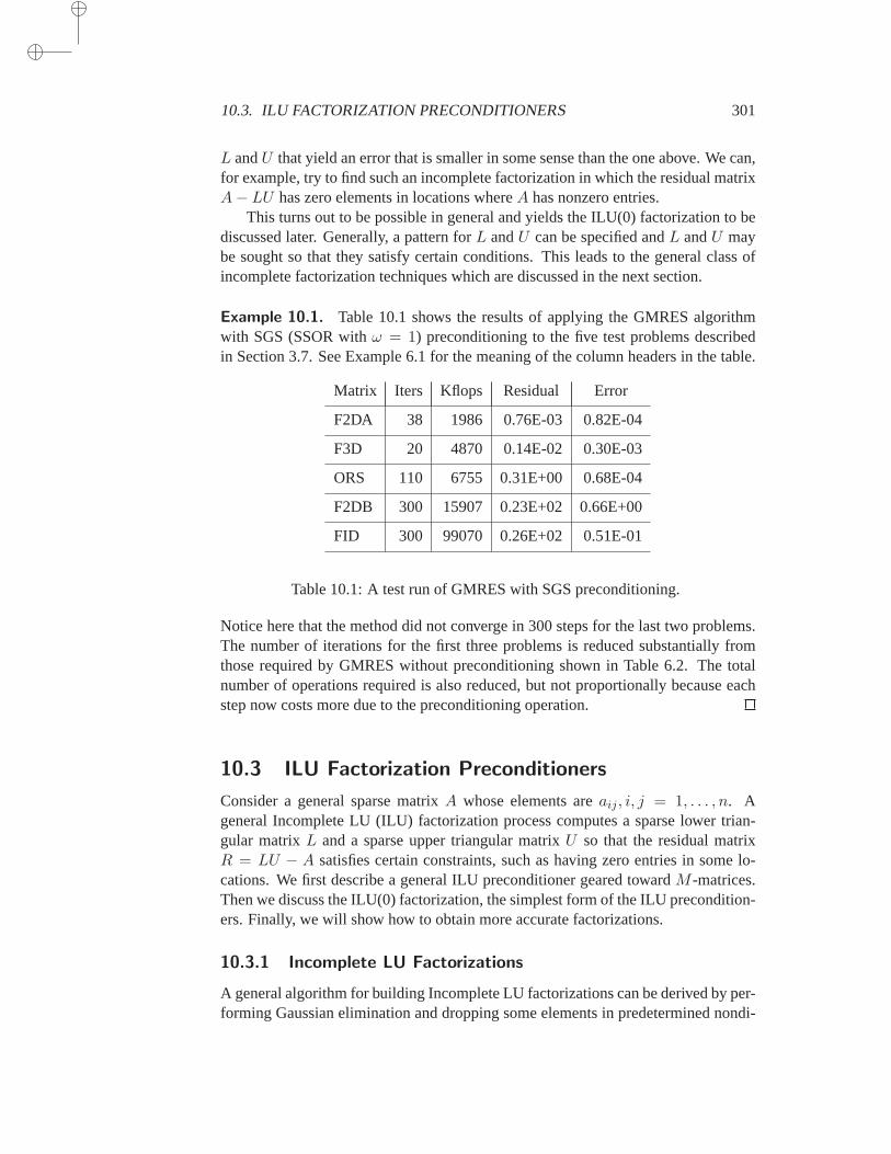
10.3. ILU FACTORIZATION PRECONDITIONERS 301
L andU that yield an error that is smaller in some sense than the one above. We can,for example, try to find such an incomplete factorization in which the residual matrixA− LU has zero elements in locations whereA has nonzero entries.
This turns out to be possible in general and yields the ILU(0) factorizationto bediscussed later. Generally, a pattern forL andU can be specified andL andU maybe sought so that they satisfy certain conditions. This leads to the generalclass ofincomplete factorization techniques which are discussed in the next section.
Example 10.1. Table 10.1 shows the results of applying the GMRES algorithmwith SGS (SSOR withω = 1) preconditioning to the five test problems describedin Section 3.7. See Example 6.1 for the meaning of the column headers in the table.
Matrix Iters Kflops Residual Error
F2DA 38 1986 0.76E-03 0.82E-04
F3D 20 4870 0.14E-02 0.30E-03
ORS 110 6755 0.31E+00 0.68E-04
F2DB 300 15907 0.23E+02 0.66E+00
FID 300 99070 0.26E+02 0.51E-01
Table 10.1: A test run of GMRES with SGS preconditioning.
Notice here that the method did not converge in 300 steps for the last two problems.The number of iterations for the first three problems is reduced substantiallyfromthose required by GMRES without preconditioning shown in Table 6.2. The totalnumber of operations required is also reduced, but not proportionally because eachstep now costs more due to the preconditioning operation.
10.3 ILU Factorization Preconditioners
Consider a general sparse matrixA whose elements areaij , i, j = 1, . . . , n. Ageneral Incomplete LU (ILU) factorization process computes a sparse lower trian-gular matrixL and a sparse upper triangular matrixU so that the residual matrixR = LU − A satisfies certain constraints, such as having zero entries in some lo-cations. We first describe a general ILU preconditioner geared toward M -matrices.Then we discuss the ILU(0) factorization, the simplest form of the ILU precondition-ers. Finally, we will show how to obtain more accurate factorizations.
10.3.1 Incomplete LU Factorizations
A general algorithm for building Incomplete LU factorizations can be derived by per-forming Gaussian elimination and dropping some elements in predetermined nondi-
302 CHAPTER 10. PRECONDITIONING TECHNIQUES
agonal positions. To analyze this process and establish existence forM -matrices, thefollowing result of Ky Fan [122] is needed.
Theorem 10.1 LetA be anM -matrix and letA1 be the matrix obtained from thefirst step of Gaussian elimination. ThenA1 is anM -matrix.
Proof. Theorem 1.32 will be used to establish that properties 1, 2, and 3 therein aresatisfied. First, consider the off-diagonal elements ofA1:
a1ij = aij −
ai1a1j
a11.
Sinceaij , ai1, a1j are nonpositive anda11 is positive, it follows thata1ij ≤ 0 for
i 6= j.Second, the fact thatA1 is nonsingular is a trivial consequence of the following
standard relation of Gaussian elimination
A = L1A1 where L1 =
[A∗,1a11
, e2, e3, . . . en
]
. (10.10)
Finally, we establish thatA−11 is nonnegative by examiningA−1
1 ej for j =1, . . . , n. For j = 1, it is clear thatA−1
1 e1 = 1a11e1 because of the structure of
A1. For the casej 6= 1, (10.10) can be exploited to yield
A−11 ej = A−1L−1
1 ej = A−1ej ≥ 0.
Therefore, all the columns ofA−11 are nonnegative by assumption and this completes
the proof.
Clearly, the(n− 1)× (n− 1) matrix obtained fromA1 by removing its first row andfirst column is also anM -matrix.
Assume now that some elements are dropped from the result of Gaussian Elim-ination outside of the main diagonal. Any element that is dropped is a nonpositiveentry which is transformed into a zero. Therefore, the resulting matrixA1 is suchthat
A1 = A1 +R,
where the elements ofR are such thatrii = 0, rij ≥ 0. Thus,
A1 ≤ A1
and the off-diagonal elements ofA1 are nonpositive. SinceA1 is anM -matrix,theorem 1.33 shows thatA1 is also anM -matrix. The process can now be repeatedon the matrixA(2 : n, 2 : n), and then continued until the incomplete factorizationof A is obtained. The above arguments shows that at each step of this construction,we obtain anM -matrix and that the process does not break down.
The elements to drop at each step have not yet been specified. This can be donestatically, by choosing some non-zero pattern in advance. The only restriction on the
10.3. ILU FACTORIZATION PRECONDITIONERS 303
zero pattern is that it should exclude diagonal elements because this assumption wasused in the above proof. Therefore, for any zero pattern setP , such that
P ⊂ (i, j) | i 6= j; 1 ≤ i, j ≤ n, (10.11)
an Incomplete LU factorization,ILUP , can be computed as follows.
ALGORITHM 10.1 General Static Pattern ILU
0. For each(i, j) ∈ P setaij = 01. Fork = 1, . . . , n− 1 Do:2. Fori = k + 1, n and if (i, k) /∈ P Do:3. aik := aik/akk
4. Forj = k + 1, . . . , n and for(i, j) /∈ P Do:5. aij := aij − aik ∗ akj
6. EndDo7. EndDo8. EndDo
The initial step (step 0) is necessary for the case, rare in practice, whenthe zeropattern ofA does not include the zero pattern defined byP . TheFor loop in line 4should be interpreted as follows:For j = k + 1, . . . , n and only for those indicesjthat are not inP execute the next line. In practice, it is wasteful to scanj from k+ 1to n because there is an inexpensive mechanism for identifying those indicesj thatare in the complement ofP . Using the above arguments, the following result can beproved.
Theorem 10.2 Let A be anM -matrix andP a given zero pattern defined as in(10.11). Then Algorithm 10.1 does not break down and produces an incompletefactorization,
A = LU −Rwhich is a regular splitting ofA.
Proof. At each step of the process, we have
Ak = Ak +Rk, Ak = LkAk−1
where, usingOk to denote a zero vector of dimensionk, andAm:n,j to denote thevector of componentsai,j , i = m, . . . , n,
Lk = I − 1
a(k)kk
(Ok
A(k + 1 : n, k)
)
eTk .
From this follow the relations
Ak = Ak +Rk = LkAk−1 +Rk.
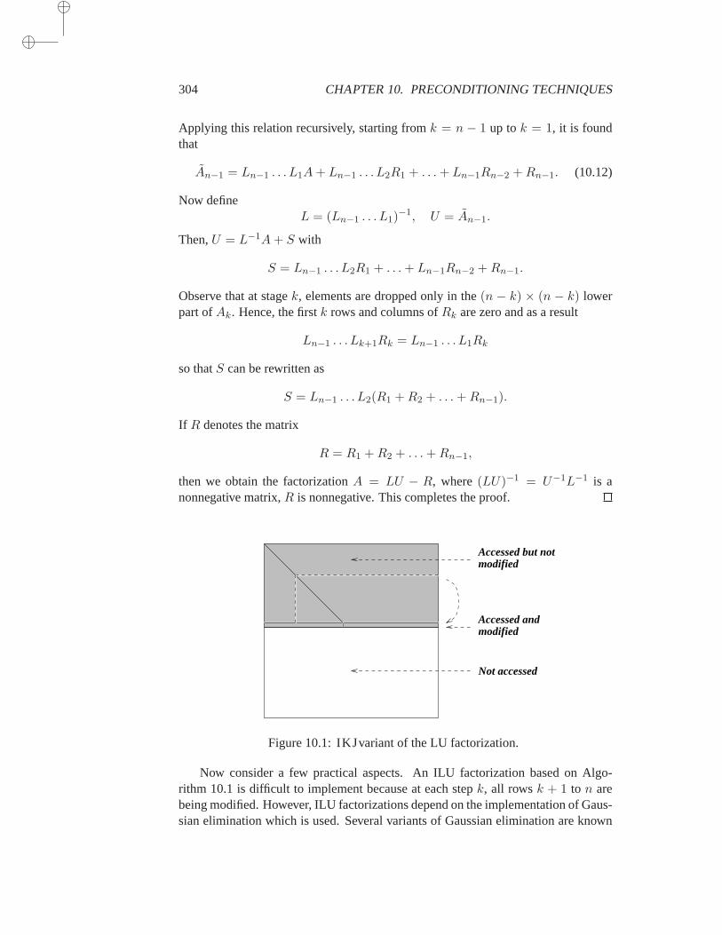
304 CHAPTER 10. PRECONDITIONING TECHNIQUES
Applying this relation recursively, starting fromk = n − 1 up tok = 1, it is foundthat
An−1 = Ln−1 . . . L1A+ Ln−1 . . . L2R1 + . . .+ Ln−1Rn−2 +Rn−1. (10.12)
Now defineL = (Ln−1 . . . L1)
−1, U = An−1.
Then,U = L−1A+ S with
S = Ln−1 . . . L2R1 + . . .+ Ln−1Rn−2 +Rn−1.
Observe that at stagek, elements are dropped only in the(n − k) × (n − k) lowerpart ofAk. Hence, the firstk rows and columns ofRk are zero and as a result
Ln−1 . . . Lk+1Rk = Ln−1 . . . L1Rk
so thatS can be rewritten as
S = Ln−1 . . . L2(R1 +R2 + . . .+Rn−1).
If R denotes the matrix
R = R1 +R2 + . . .+Rn−1,
then we obtain the factorizationA = LU − R, where(LU)−1 = U−1L−1 is anonnegative matrix,R is nonnegative. This completes the proof.
Not accessed
Accessed but not
Accessed and modified
modified
Figure 10.1: IKJvariant of the LU factorization.
Now consider a few practical aspects. An ILU factorization based on Algo-rithm 10.1 is difficult to implement because at each stepk, all rowsk + 1 to n arebeing modified. However, ILU factorizations depend on the implementation of Gaus-sian elimination which is used. Several variants of Gaussian elimination are known
10.3. ILU FACTORIZATION PRECONDITIONERS 305
which depend on the order of the three loops associated with the control variablesi,j, andk in the algorithm. Thus, Algorithm 10.1 is derived from what is known as thek, i, j variant. In the context of Incomplete LU factorization, the variant that is mostcommonly used for a row-contiguous data structure is thei, k, j variant, describednext for dense matrices.
ALGORITHM 10.2 Gaussian Elimination – IKJ Variant
1. Fori = 2, . . . , n Do:2. Fork = 1, . . . , i− 1 Do:3. aik := aik/akk
4. Forj = k + 1, . . . , n Do:5. aij := aij − aik ∗ akj
6. EndDo7. EndDo8. EndDo
The above algorithm is in place in the sense that thei-th row ofA can be over-written by thei-th rows of theL andU matrices of the factorization (sinceL is unitlower triangular, its diagonal entries need not be stored). Stepi of the algorithm gen-erates thei-th row ofL and thei-th row ofU at the same time. The previous rows1, 2, . . . , i − 1 of L andU are accessed at stepi but they are not modified. This isillustrated in Figure 10.1.
Adapting this version for sparse matrices is easy because the rows ofL andUare generated in succession. These rows can be computed one at a time and accu-mulated in a row-oriented data structure such as the CSR format. This constitutes animportant advantage. Based on this, the general ILU factorization takes the followingform.
ALGORITHM 10.3 General ILU Factorization, IKJVersion
1. Fori = 2, . . . , n Do:2. Fork = 1, . . . , i− 1 and if (i, k) /∈ P Do:3. aik := aik/akk
4. Forj = k + 1, . . . , n and for(i, j) /∈ P , Do:5. aij := aij − aikakj .6. EndDo7. EndDo8. EndDo
It is not difficult to see that this more practical IKJvariant of ILU is equivalent to theKIJversion which can be defined from Algorithm 10.1.
Proposition 10.3 LetP be a zero pattern satisfying the condition (10.11). Then theILU factors produced by the KIJ-based Algorithm 10.1 and the IKJ-based Algo-rithm 10.3 are identical if they can both be computed.
306 CHAPTER 10. PRECONDITIONING TECHNIQUES
Proof. Algorithm 10.3 is obtained from Algorithm 10.1 by switching the order of theloopsk andi. To see that this gives indeed the same result, reformulate the first twoloops of Algorithm 10.1 as
Fork = 1, n Do:For i = 1, n Do:
if k < i and for(i, k) /∈ P Do:ope(row(i),row(k)). . . . . .
in whichope(row(i),row(k))is the operation represented by lines 3 through 6 of bothAlgorithm 10.1 and Algorithm 10.3. In this form, it is clear that thek andi loopscan be safely permuted. Then the resulting algorithm can be reformulated to yieldexactly Algorithm 10.3.
Note that this is only true for a static pattern ILU. If the pattern is dynamically de-termined as the Gaussian elimination algorithm proceeds, then the patterns obtainedwith different versions of GE may be different.
It is helpful to interpret the result of one incomplete elimination step. Denotingby li∗, ui∗, andai∗ thei-th rows ofL,U , andA, respectively, then thek-loop startingat line 2 of Algorithm 10.3 can be interpreted as follows. Initially, we haveui∗ = ai∗.Then, each elimination step is an operation of the form
ui∗ := ui∗ − likuk∗.
However, this operation is performed only on the nonzero pattern, i.e., the comple-ment ofP . This means that, in reality, the elimination step takes the form
ui∗ := ui∗ − likuk∗ + r(k)i∗ ,
in which r(k)ij is zero when(i, j) /∈ P and equalslikukj when(i, j) ∈ P . Thus,
the rowr(k)i∗ cancels out the termslikukj that would otherwise be introduced in the
zero pattern. In the end the following relation is obtained:
ui∗ = ai∗ −i−1∑
k=1
(
likuk∗ − r(k)i∗
)
.
Note thatlik = 0 for (i, k) ∈ P . We now sum up all ther(k)i∗ ’s and define
ri∗ =i−1∑
k=1
r(k)i∗ . (10.13)
The rowri∗ contains the elements that fall inside theP pattern at the completion ofthek-loop. Using the fact thatlii = 1, we obtain the relation,
ai∗ =i∑
k=1
likuk∗ − ri∗. (10.14)
Therefore, the following simple property can be stated.
10.3. ILU FACTORIZATION PRECONDITIONERS 307
Proposition 10.4 Algorithm 10.3 produces factorsL andU such that
A = LU −R
in which−R is the matrix of the elements that are dropped during the incompleteelimination process. When(i, j) ∈ P , an entryrij of R is equal to the value of−aij obtained at the completion of thek loop in Algorithm 10.3. Otherwise,rij iszero.
10.3.2 Zero Fill-in ILU (ILU(0))
The Incomplete LUfactorization technique with no fill-in, denoted by ILU(0), takesthe zero patternP to be precisely the zero pattern ofA. In the following, we denoteby bi,∗ the i-th row of a given matrixB, and byNZ(B), the set of pairs(i, j), 1 ≤i, j ≤ n such thatbi,j 6= 0. The ILU(0) factorization is best illustrated by the case forwhich it was discovered originally, namely, for 5-point and 7-point matrices relatedto finite difference discretization of elliptic PDEs. Consider one such matrixA asillustrated in the bottom left corner of Figure 10.2.
TheA matrix represented in this figure is a 5-point matrix of sizen = 32 corre-sponding to annx × ny = 8× 4 mesh. Consider now any lower triangular matrixLwhich has the same structure as the lower part ofA, and any matrixU which has thesame structure as that of the upper part ofA. Two such matrices are shown at the topof Figure 10.2. If the productLU were performed, the resulting matrix would havethe pattern shown in the bottom right part of the figure. It is impossible in generalto matchA with this product for anyL andU . This is due to the extra diagonals inthe product, namely, the diagonals with offsetsnx − 1 and−nx + 1. The entries inthese extra diagonals are calledfill-in elements. However, if these fill-in elements areignored, then it is possible to findL andU so that their product is equal toA in theother diagonals.
The ILU(0) factorization has just been defined in general terms: Any pair ofmatricesL (unit lower triangular) andU (upper triangular) so that the elements ofA − LU are zero in the locations ofNZ(A). These constraints do not define theILU(0) factors uniquely since there are, in general, infinitely many pairs of matricesL andU which satisfy these requirements. However, the standard ILU(0) is definedconstructively using Algorithm 10.3 with the patternP equal to the zero pattern ofA.
ALGORITHM 10.4 ILU(0)
1. Fori = 2, . . . , n Do:2. Fork = 1, . . . , i− 1 and for(i, k) ∈ NZ(A) Do:3. Computeaik = aik/akk
4. Forj = k + 1, . . . , n and for(i, j) ∈ NZ(A), Do:5. Computeaij := aij − aikakj .6. EndDo7. EndDo
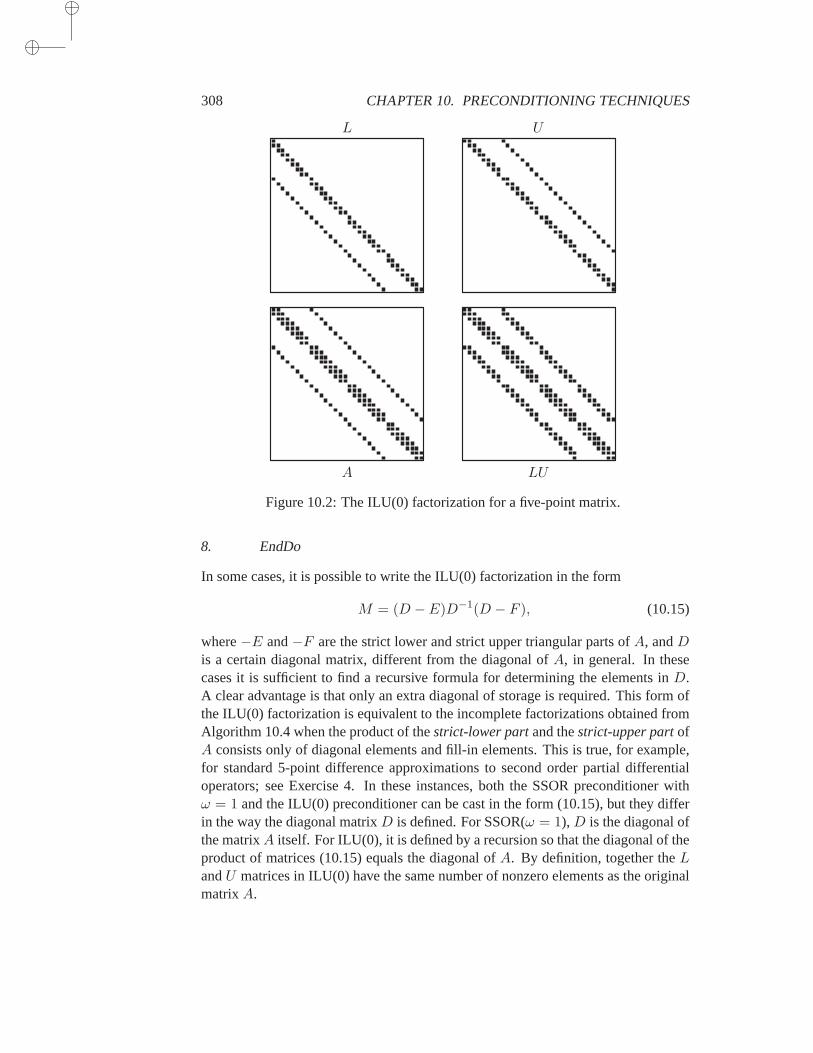
308 CHAPTER 10. PRECONDITIONING TECHNIQUES
A
L U
LU
Figure 10.2: The ILU(0) factorization for a five-point matrix.
8. EndDo
In some cases, it is possible to write the ILU(0) factorization in the form
M = (D − E)D−1(D − F ), (10.15)
where−E and−F are the strict lower and strict upper triangular parts ofA, andDis a certain diagonal matrix, different from the diagonal ofA, in general. In thesecases it is sufficient to find a recursive formula for determining the elementsin D.A clear advantage is that only an extra diagonal of storage is required. This form ofthe ILU(0) factorization is equivalent to the incomplete factorizations obtained fromAlgorithm 10.4 when the product of thestrict-lower partand thestrict-upper partofA consists only of diagonal elements and fill-in elements. This is true, for example,for standard 5-point difference approximations to second order partial differentialoperators; see Exercise 4. In these instances, both the SSOR preconditioner withω = 1 and the ILU(0) preconditioner can be cast in the form (10.15), but theydifferin the way the diagonal matrixD is defined. For SSOR(ω = 1),D is the diagonal ofthe matrixA itself. For ILU(0), it is defined by a recursion so that the diagonal of theproduct of matrices (10.15) equals the diagonal ofA. By definition, together theLandU matrices in ILU(0) have the same number of nonzero elements as the originalmatrixA.
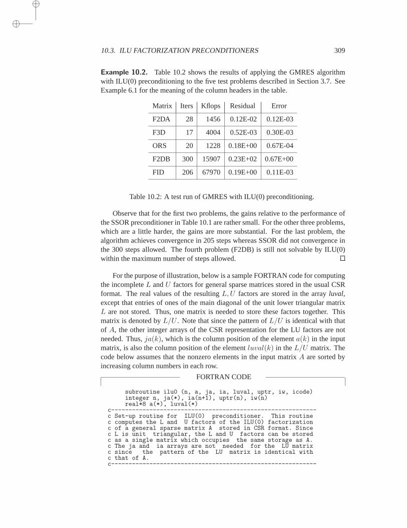
10.3. ILU FACTORIZATION PRECONDITIONERS 309
Example 10.2. Table 10.2 shows the results of applying the GMRES algorithmwith ILU(0) preconditioning to the five test problems described in Section 3.7.SeeExample 6.1 for the meaning of the column headers in the table.
Matrix Iters Kflops Residual Error
F2DA 28 1456 0.12E-02 0.12E-03
F3D 17 4004 0.52E-03 0.30E-03
ORS 20 1228 0.18E+00 0.67E-04
F2DB 300 15907 0.23E+02 0.67E+00
FID 206 67970 0.19E+00 0.11E-03
Table 10.2: A test run of GMRES with ILU(0) preconditioning.
Observe that for the first two problems, the gains relative to the performance ofthe SSOR preconditioner in Table 10.1 are rather small. For the other three problems,which are a little harder, the gains are more substantial. For the last problem, thealgorithm achieves convergence in 205 steps whereas SSOR did not convergence inthe 300 steps allowed. The fourth problem (F2DB) is still not solvable by ILU(0)within the maximum number of steps allowed.
For the purpose of illustration, below is a sample FORTRAN code for computingthe incompleteL andU factors for general sparse matrices stored in the usual CSRformat. The real values of the resultingL,U factors are stored in the arrayluval,except that entries of ones of the main diagonal of the unit lower triangularmatrixL are not stored. Thus, one matrix is needed to store these factors together. Thismatrix is denoted byL/U . Note that since the pattern ofL/U is identical with thatof A, the other integer arrays of the CSR representation for the LU factors are notneeded. Thus,ja(k), which is the column position of the elementa(k) in the inputmatrix, is also the column position of the elementluval(k) in theL/U matrix. Thecode below assumes that the nonzero elements in the input matrixA are sorted byincreasing column numbers in each row.
FORTRAN CODE
subroutine ilu0 (n, a, ja, ia, luval, uptr, iw, icode)integer n, ja(*), ia(n+1), uptr(n), iw(n)real*8 a(*), luval(*)
c-----------------------------------------------------------c Set-up routine for ILU(0) preconditioner. This routinec computes the L and U factors of the ILU(0) factorizationc of a general sparse matrix A stored in CSR format. Sincec L is unit triangular, the L and U factors can be storedc as a single matrix which occupies the same storage as A.c The ja and ia arrays are not needed for the LU matrixc since the pattern of the LU matrix is identical withc that of A.c-----------------------------------------------------------

310 CHAPTER 10. PRECONDITIONING TECHNIQUES
c INPUT:c ------c n = dimension of matrixc a, ja, ia = sparse matrix in general sparse storage formatc iw = integer work array of length nc OUTPUT:c -------c luval = L/U matrices stored together. On return luval,c ja, ia is the combined CSR data structure forc the LU factorsc uptr = pointer to the diagonal elements in the CSRc data structure luval, ja, iac icode = integer indicating error code on returnc icode = 0: normal returnc icode = k: encountered a zero pivot at step kcc-----------------------------------------------------------c initialize work array iw to zero and luval array to a
do 30 i = 1, ia(n+1)-1luval(i) = a(i)
30 continuedo 31 i=1, n
iw(i) = 031 continuec----------------------- Main loop
do 500 k = 1, nj1 = ia(k)j2 = ia(k+1)-1do 100 j=j1, j2
iw(ja(j)) = j100 continue
j=j1150 jrow = ja(j)c----------------------- Exit if diagonal element is reached
if (jrow .ge. k) goto 200c----------------------- Compute the multiplier for jrow.
tl = luval(j)*luval(uptr(jrow))luval(j) = tl
c----------------------- Perform linear combinationdo 140 jj = uptr(jrow)+1, ia(jrow+1)-1
jw = iw(ja(jj))if (jw .ne. 0) luval(jw)=luval(jw)-tl*luval(jj)
140 continuej=j+1if (j .le. j2) goto 150
c----------------------- Store pointer to diagonal element200 uptr(k) = j
if (jrow .ne. k .or. luval(j) .eq. 0.0d0) goto 600luval(j) = 1.0d0/luval(j)
c----------------------- Refresh all entries of iw to zero.do 201 i = j1, j2
iw(ja(i)) = 0201 continue500 continuec----------------------- Normal return
icode = 0return
c----------------------- Error: zero pivot600 icode = k
returnend
10.3. ILU FACTORIZATION PRECONDITIONERS 311
10.3.3 Level of Fill and ILU(p)
The accuracy of the ILU(0) incomplete factorization may be insufficient to yield anadequate rate of convergence as shown in Example 10.2. More accurateIncompleteLU factorizations are often more efficient as well as more reliable. These more ac-curate factorizations will differ from ILU(0) by allowing some fill-in. Thus,ILU(1)keeps the “first order fill-ins,” a term which will be explained shortly.
To illustrate ILU(p) with the same example as before, the ILU(1) factorizationresults from takingP to be the zero pattern of the productLU of the factorsL,Uobtained from ILU(0). This pattern is shown at the bottom right of Figure 10.2. Pre-tend that the original matrix has this “augmented” patternNZ1(A). In other words,the fill-in positions created in this product belong to the augmented patternNZ1(A),but their actual values are zero. The new pattern of the matrixA is shown at thebottom left part of Figure 10.3. The factorsL1 andU1 of the ILU(1) factorization areobtained by performing an ILU(0) factorization on this “augmented pattern”matrix.The patterns ofL1 andU1 are illustrated at the top of Figure 10.3. The new LUmatrix shown at the bottom right of the figure has now two additional diagonalsinthe lower and upper parts.
One problem with the construction defined in this illustration is that it does notextend to general sparse matrices. It can be generalized by introducingthe concept oflevel of fill. A level of fill is attributed to each element that is processed by Gaussianelimination, and dropping will be based on the value of the level of fill. Algorithm10.2 will be used as a model, although any other form of GE can be used.
The rationale is that the level of fill should be indicative of the size: the higherthe level, the smaller the elements. A very simple model is employed to justify thedefinition: A size ofǫk is attributed to any element whose level of fill isk, whereǫ < 1. Initially, a nonzero element has a level of fill of one (this will be changedlater) and a zero element has a level of fill of∞. An elementaij is updated in line 5of Algorithm 10.2 by the formula
aij = aij − aik × akj . (10.16)
If levij is the current level of the elementaij , then our model tells us that the size ofthe updated element should be
size(aij) := ǫlevij − ǫlevik × ǫlevkj = ǫlevij − ǫlevik+levkj .
Therefore, roughly speaking, the size ofaij will be the maximum of the twosizesǫlevij andǫlevik+levkj , and it is natural to define the new level of fill as,
levij := minlevij , levik + levkj.In the common definition used in the literature, all the levels of fill are actually shiftedby−1 from the definition used above. This is purely for convenience of notationandto conform with the definition used for ILU(0). Thus, initiallylevij = 0 if aij 6= 0,andlevij =∞ otherwise. Thereafter, define recursively
levij = minlevij , levik + levkj + 1.

312 CHAPTER 10. PRECONDITIONING TECHNIQUES
AugmentedA
L1 U1
L1U1
Figure 10.3: The ILU(1) factorization for a five-point matrix.
Definition 10.5 The initial level of fill of an elementaij of a sparse matrixA isdefined by
levij =
0 if aij 6= 0, or i = j∞ otherwise.
Each time this element is modified in line 5 of Algorithm 10.2, its level of fill must beupdated by
levij = minlevij , levik + levkj + 1. (10.17)
Observe that the level of fill of an element will never increase during the elimination.Thus, ifaij 6= 0 in the original matrixA, then the element in locationi, j will have alevel of fill equal to zero throughout the elimination process.
An alternative way of interpreting the above definition of fill-level can be drawnfrom the graph model of Gaussian elimination, which is a standard tool used insparsedirect solvers. Consider the adjacency graphG(A) = (V,E) of the matrixA. Atthe completion of stepk − 1 of Gaussian elimination, nodes1, 2, . . . , k − 1 havebeen eliminated. LetVk−1 the set of thek − 1 vertices that are eliminated so far andlet vi, vj two vertices not inVk, i.e., such thati, j > k. The vertexvi is said to bereachable from the vertexvj throughVk−1 if there is a path in the (original) graphG(A) which connectsvi to vj , in which all intermediate vertices are inVk−1. The setof all nodesv that are reachable fromu throughVk−1 is denoted byReach(u, Vk−1).

10.3. ILU FACTORIZATION PRECONDITIONERS 313
i
V k-1
jk
Figure 10.4: Shortest path fromj to j whenk is added toVk−1.
The fill-level of (i, j) at stepk − 1 is simply the length of the shortest path throughVk−1 betweenvi andvj , minus 1. The initial fill-levels are defined as before, to bezero when(i, j) ∈ V0 and infinity otherwise. At the next step (k), nodek will beadded toVk−1 to getVk. Now more paths are available and so the path lengths maybe shortened by taking paths that go through the new nodevk.
If we use the shifted levels (all levels are increased by one, so that thelev(i, j) isthe actual minimum path length) then, the shortest path is now the shortest of theoldshortest path and new possible paths throughvk. A path throughvk is a path fromi to vk continued by a path fromvk to j. Therefore, the new pathlength is indeedminlevij , levik + levkj. This is illustrated in Figure 10.4.
Another useful concept in sparse direct solution methods is that offill-path,which is a path between two verticesi andj, such that all the vertices in the path,except the end pointsi andj, are numbered less thani andj. The following result iswell-known in sparse direct solution methods.
Theorem 10.6 There is a fill-in in entry(i, j) at the completion of the Gaussianelimination process if and only if, there exists a fill-path betweeni andj.
For a proof see [144, 233]. As it turns out, a fill-in entry which has level-of-fill valuep corresponds to fill-paths whose length isp+ 1.
Theorem 10.7 At the completion of the ILU process, a fill-in entry in position(i, j)has level-of-fill valuep if and only if there exists a fill-path of lengthp+ 1 betweeniandj.
Proof. If there is a fill-path of lengthp, then from what said above on reachable sets,it is clear thatlev(aij) ≤ p. However,lev(aij) cannot be< p, otherwise at some stepk we would have a path betweeni andj that is of length< p. Since path lengths donot increase, this would lead to a contradiction. The converse is also true.If lev(aij)is equal top then at the last stepk whenlev(aij) was modified there was a path oflengthp betweeni andj.
The above systematic definition gives rise to a natural strategy for discarding ele-ments. In ILU(p), all fill-in elements whose level of fill does not exceedp are kept.
314 CHAPTER 10. PRECONDITIONING TECHNIQUES
So using the definition of zero patterns introduced earlier, the zero patternfor ILU(p)is the set
Pp = (i, j) | levij > p,wherelevij is the level of fill value after all updates (10.17) have been performed.The casep = 0 coincides with the ILU(0) factorization and is consistent with theearlier definition.
Since fill levels are is essentially path-lengths in the graph, they are boundedfrom above byδ(G)+1 where the diameterδ(G) of a graphG is maximum possibledistanced(x, y) between two verticesx andy of the graph
δ(G) = maxd(x, y) | x ∈ V, y ∈ V .
Recall that the distanced(x, y) between verticesx andy in the graph is the length ofthe shortest path betweenx andy.
Definition 10.5 of fill levels is not the only one used in practice. An alternativedefinition replaces the updating formula (10.17) by
levij = minlevij ,maxlevik, levkj+ 1. (10.18)
In practical implementations of the ILU(p) factorization it is common to separatethe symbolic phase (where the structure of theL andU factors are determined) fromthe numerical factorization, when the numerical values are computed. Here, a variantis described which does not separate these two phases. In the following description,ai∗ denotes thei-th row of the matrixA, andaij the(i, j)-th entry ofA.
ALGORITHM 10.5 ILU(p)
1. For all nonzero elementsaij definelev(aij) = 02. Fori = 2, . . . , n Do:3. For eachk = 1, . . . , i− 1 and forlev(aik) ≤ p Do:4. Computeaik := aik/akk
5. Computeai∗ := ai∗ − aikak∗.6. Update the levels of fill of the nonzeroai,j ’s using (10.17)7. EndDo8. Replace any element in rowi with lev(aij) > p by zero9. EndDo
There are a number of drawbacks to the above algorithm. First, the amount of fill-inand computational work for obtaining the ILU(p) factorization is not predictable forp > 0. Second, the cost of updating the levels can be high. Most importantly, thelevel of fill-in for indefinite matrices may not be a good indicator of the size of theelements that are being dropped. Thus, the algorithm may drop large elementsandresult in an inaccurate incomplete factorization, in thatR = LU − A is not small.Experience reveals thaton the averagethis will lead to a larger number of iterationsto achieve convergence. The techniques which will be described in Section 10.4 havebeen developed to remedy these difficulties by producing incomplete factorizationswith small errorR and controlled fill-in.
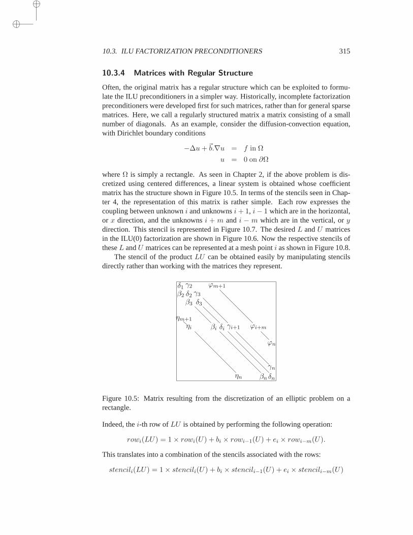
10.3. ILU FACTORIZATION PRECONDITIONERS 315
10.3.4 Matrices with Regular Structure
Often, the original matrix has a regular structure which can be exploited to formu-late the ILU preconditioners in a simpler way. Historically, incomplete factorizationpreconditioners were developed first for such matrices, rather than for general sparsematrices. Here, we call a regularly structured matrix a matrix consisting of a smallnumber of diagonals. As an example, consider the diffusion-convection equation,with Dirichlet boundary conditions
−∆u+~b.∇u = f in Ω
u = 0 on ∂Ω
whereΩ is simply a rectangle. As seen in Chapter 2, if the above problem is dis-cretized using centered differences, a linear system is obtained whose coefficientmatrix has the structure shown in Figure 10.5. In terms of the stencils seen in Chap-ter 4, the representation of this matrix is rather simple. Each row expresses thecoupling between unknowni and unknownsi+ 1, i− 1 which are in the horizontal,or x direction, and the unknownsi + m andi − m which are in the vertical, orydirection. This stencil is represented in Figure 10.7. The desiredL andU matricesin the ILU(0) factorization are shown in Figure 10.6. Now the respective stencils oftheseL andU matrices can be represented at a mesh pointi as shown in Figure 10.8.
The stencil of the productLU can be obtained easily by manipulating stencilsdirectly rather than working with the matrices they represent.
δ1 γ2 ϕm+1
β2 δ2 γ3
β3 δ3
ηm+1
ηi βi δi γi+1 ϕi+m
ϕn
ηn βn δn
γn
Figure 10.5: Matrix resulting from the discretization of an elliptic problem on arectangle.
Indeed, thei-th row ofLU is obtained by performing the following operation:
rowi(LU) = 1× rowi(U) + bi × rowi−1(U) + ei × rowi−m(U).
This translates into a combination of the stencils associated with the rows:
stencili(LU) = 1× stencili(U) + bi × stencili−1(U) + ei × stencili−m(U)
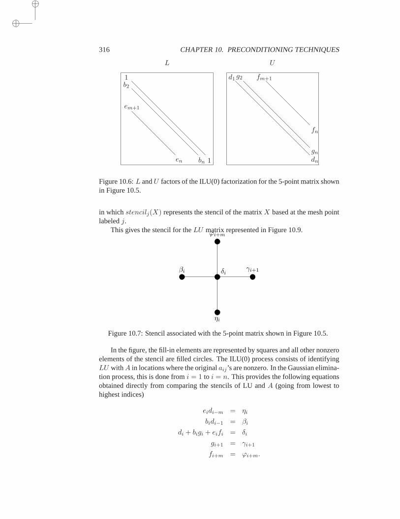
316 CHAPTER 10. PRECONDITIONING TECHNIQUES
1b2
bn 1
em+1
en
d1 g2
dn
gn
fm+1
fn
L U
Figure 10.6:L andU factors of the ILU(0) factorization for the 5-point matrix shownin Figure 10.5.
in whichstencilj(X) represents the stencil of the matrixX based at the mesh pointlabeledj.
This gives the stencil for theLU matrix represented in Figure 10.9.
γi+1δiβi
ηi
ϕi+m
Figure 10.7: Stencil associated with the 5-point matrix shown in Figure 10.5.
In the figure, the fill-in elements are represented by squares and all othernonzeroelements of the stencil are filled circles. The ILU(0) process consists of identifyingLU withA in locations where the originalaij ’s are nonzero. In the Gaussian elimina-tion process, this is done fromi = 1 to i = n. This provides the following equationsobtained directly from comparing the stencils of LU andA (going from lowest tohighest indices)
eidi−m = ηi
bidi−1 = βi
di + bigi + eifi = δi
gi+1 = γi+1
fi+m = ϕi+m.
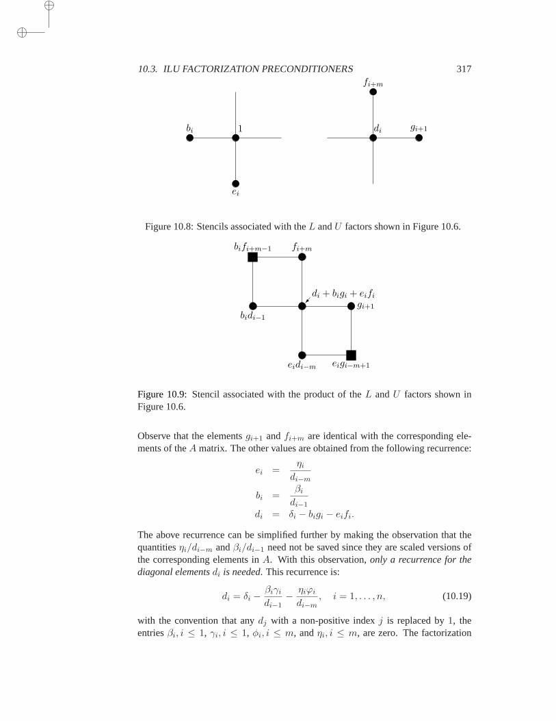
10.3. ILU FACTORIZATION PRECONDITIONERS 317
ei
1bi
fi+m
di gi+1
Figure 10.8: Stencils associated with theL andU factors shown in Figure 10.6.
gi+1
di + bigi + eifi
bidi−1
fi+m
eidi−m
bifi+m−1
eigi−m+1
Figure 10.9:Stencil associated with the product of theL andU factors shown inFigure 10.6.
Observe that the elementsgi+1 andfi+m are identical with the corresponding ele-ments of theA matrix. The other values are obtained from the following recurrence:
ei =ηi
di−m
bi =βi
di−1
di = δi − bigi − eifi.
The above recurrence can be simplified further by making the observationthat thequantitiesηi/di−m andβi/di−1 need not be saved since they are scaled versions ofthe corresponding elements inA. With this observation,only a recurrence for thediagonal elementsdi is needed. This recurrence is:
di = δi −βiγi
di−1− ηiϕi
di−m, i = 1, . . . , n, (10.19)
with the convention that anydj with a non-positive indexj is replaced by1, theentriesβi, i ≤ 1, γi, i ≤ 1, φi, i ≤ m, andηi, i ≤ m, are zero. The factorization

318 CHAPTER 10. PRECONDITIONING TECHNIQUES
obtained takes the form
M = (D − E)D−1(D − F ) (10.20)
in which−E is the strict lower diagonal ofA, −F is the strict upper triangular partof A, andD is the diagonal obtained with the above recurrence. Note that an ILU(0)based on the IKJversion of Gaussian elimination would give the same result.
For a general sparse matrixA with irregular structure, one can also determinea preconditioner in the form (10.20) by requiring only that the diagonal elementsof M match those ofA (see Exercise 10). However, this will not give the sameILU factorization as the one based on the IKJvariant of Gaussian eliminationseenearlier. Why the ILU(0) factorization gives rise to the same factorization asthat of(10.20) is simple to understand: The product ofL andU does not change the valuesof the existing elements in the upper part, except for the diagonal. This also can beinterpreted on the adjacency graph of the matrix.
This approach can now be extended to determine the ILU(1) factorization as wellas factorizations with higher levels of fill. The stencils of theL andU matrices inthe ILU(1) factorization are the stencils of the lower part and upper partsof the LUmatrix obtained from ILU(0). These are shown in Figure 10.10. In the illustration,the meaning of a given stencil is not in the usual graph theory sense. Instead, allthe marked nodes at a stencil based at nodei represent those nodes coupled withunknowni by an equation. Thus, all the filled circles in the picture are adjacent tothe central node. Proceeding as before and combining stencils to form thestencilassociated with the LU matrix, we obtain the stencil shown in Figure 10.11.
ei
1bi
ci
fi+m
di gi+1
hi+m−1
Figure 10.10:Stencils of theL andU factors for the ILU(0) factorization of thematrix represented by the stencil of Figure 10.9.
As before, the fill-in elements are represented by squares and all other elementsare filled circles. A typical row of the matrix associated with the above stencil hasnine nonzero elements. Two of these are fill-ins, i.e., elements that fall outsidetheoriginal structure of theL andU matrices. It is now possible to determine a recur-rence relation for obtaining the entries ofL andU . There are seven equations in allwhich, starting from the bottom, are
eidi−m = ηi
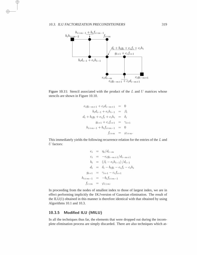
10.3. ILU FACTORIZATION PRECONDITIONERS 319
bihi+m−2
hi+m−1 + bifi+m−1
? fi+m
bidi−1 + eihi−1
di + bigi + eifi + cihi
gi+1 + cifi+1
eidi−meigi−m+1 + cidi−m+1
6 cigi−m+1
Figure 10.11:Stencil associated with the product of theL andU matrices whosestencils are shown in Figure 10.10.
eigi−m+1 + cidi−m+1 = 0
bidi−1 + eihi−1 = βi
di + bigi + eifi + cihi = δi
gi+1 + cifi+1 = γi+1
hi+m−1 + bifi+m−1 = 0
fi+m = ϕi+m.
This immediately yields the following recurrence relation for the entries of theL andU factors:
ei = ηi/di−m
ci = −eigi−m+1/di−m+1
bi = (βi − eihi−1) /di−1
di = δi − bigi − eifi − cihi
gi+1 = γi+1 − cifi+1
hi+m−1 = −bifi+m−1
fi+m = ϕi+m.
In proceeding from the nodes of smallest index to those of largest index,we are ineffect performing implicitly the IKJversion of Gaussian elimination. The resultofthe ILU(1) obtained in this manner is therefore identical with that obtained by usingAlgorithms 10.1 and 10.3.
10.3.5 Modified ILU (MILU)
In all the techniques thus far, the elements that were dropped out during the incom-plete elimination process are simply discarded. There are also techniques which at-
320 CHAPTER 10. PRECONDITIONING TECHNIQUES
tempt to reduce the effect of dropping bycompensatingfor the discarded entries. Forexample, a popular strategy is to add up all the elements that have been dropped atthe completion of thek-loop of Algorithm 10.3. Then this sum is subtracted from thediagonal entry inU . Thisdiagonal compensationstrategy gives rise to the ModifiedILU (MILU) factorization.
Thus, in equation (10.13), the final rowui∗ obtained after completion of thek-loop of Algorithm 10.3 undergoes one more modification, namely,
uii := uii − (ri∗e)
in whiche ≡ (1, 1, . . . , 1)T . Note thatri∗ is a row andri∗e is the sum of the elementsin this row, i.e., itsrow sum. The above equation can be rewritten in row form asui∗ := ui∗ − (ri∗e)eTi and equation (10.14) becomes
ai∗ =i∑
k=1
likuk∗ + (ri∗e)eTi − ri∗. (10.21)
Observe that
ai∗e =i∑
k=1
likuk∗e+ (ri∗e)eTi e− ri∗e =
i−1∑
k=1
likuk∗e = LU e.
This establishes thatAe = LUe. As a result, this strategy guarantees that the rowsums ofA are equal to those ofLU . For PDEs, the vector of all ones representsthe discretization of a constant function. This additional constraint forces the ILUfactorization to be exact for constant functions in some sense. Therefore, it is notsurprising that often the algorithm does well for such problems. For otherproblemsor problems with discontinuous coefficients, MILU algorithms usually are notbetterthan their ILU counterparts, in general.
Example 10.3. For regularly structured matrices there are two elements droppedat thei-th step of ILU(0). These arebifi+m−1 andeigi−m+1 located on the north-west and south-east corners of the stencil, respectively. Thus, the row sumri,∗eassociated with stepi is
si =βiφi+m−1
di−1+ηiγm−i+1
di−m
and the MILU variant of the recurrence (10.19) is
si =βiφi+m−1
di−1+ηiγm−i+1
di−m
di = δi −βiγi
di−1− ηiϕi
di−m− si.
10.4. THRESHOLD STRATEGIES AND ILUT 321
The new ILU factorization is now such thatA = LU − R in which according to(10.21) thei-th row of the new remainder matrixR is given by
r(new)i,∗ = (ri∗e)e
Ti − ri∗
whose row sum is zero.This generic idea of lumping together all the elements dropped in the elimination
process and adding them to the diagonal ofU can be used forany form of ILUfactorization. In addition, there are variants of diagonal compensation in which onlya fraction of the dropped elements are added to the diagonal. Thus, the termsi inthe above example would be replaced byωsi before being added touii, whereωis typically between 0 and 1. Other strategies distribute the sumsi among nonzeroelements ofL andU , other than the diagonal.
10.4 Threshold Strategies and ILUT
Incomplete factorizations which rely on the levels of fill are blind to numerical valuesbecause elements that are dropped depend only on the structure ofA. This can causesome difficulties for realistic problems that arise in many applications. A few alter-native methods are available which are based on dropping elements in the Gaussianelimination process according to their magnitude rather than their locations. Withthese techniques, the zero patternP is determined dynamically. The simplest wayto obtain an incomplete factorization of this type is to take a sparse direct solverand modify it by adding lines of code which will ignore “small” elements. How-ever, most direct solvers have a complex implementation involving several layers ofdata structures that may make this approach ineffective. It is desirable to develop astrategy which is more akin to the ILU(0) approach. This section describesone suchtechnique.
10.4.1 The ILUT Approach
A generic ILU algorithm with threshold can be derived from the IKJversion of Gaus-sian elimination, Algorithm 10.2, by including a set of rules for dropping small el-ements. In what follows,applying a dropping rule to an elementwill only meanreplacing the element by zero if it satisfies a set of criteria. A dropping rule can beapplied to a whole row by applying the same rule to all the elements of the row. Inthe following algorithm,w is a full-length working row which is used to accumulatelinear combinations of sparse rows in the elimination andwk is thek-th entry of thisrow. As usual,ai∗ denotes thei-th row ofA.
ALGORITHM 10.6 ILUT
1. Fori = 1, . . . , n Do:2. w := ai∗3. Fork = 1, . . . , i− 1 and whenwk 6= 0 Do:4. wk := wk/akk
322 CHAPTER 10. PRECONDITIONING TECHNIQUES
5. Apply a dropping rule towk
6. If wk 6= 0 then7. w := w − wk ∗ uk∗8. EndIf9. EndDo
10. Apply a dropping rule to roww11. li,j := wj for j = 1, . . . , i− 112. ui,j := wj for j = i, . . . , n13. w := 014. EndDo
Now consider the operations involved in the above algorithm. Line 7 is a sparseupdate operation. A common implementation of this is to use a full vector forw anda companion pointer which points to the positions of its nonzero elements. Similarly,lines 11 and 12 are sparse-vector copy operations. The vectorw is filled with a fewnonzero elements after the
completion of each outer loopi, and therefore it is necessary to zero out thoseelements at the end of the Gaussian elimination loop as is done in line 13. This is asparseset-to-zerooperation.
ILU(0) can be viewed as a particular case of the above algorithm. The droppingrule for ILU(0) is to drop elements that are in positions not belonging to the originalstructure of the matrix.
In the factorization ILUT(p, τ ), the following rule is used.
1. In line 5, an elementwk is dropped (i.e., replaced by zero) if it is less than therelative toleranceτi obtained by multiplyingτ by the original norm of thei-throw (e.g., the 2-norm).
2. In line 10, a dropping rule of a different type is applied. First, drop againany element in the row with a magnitude that is below the relative toleranceτi. Then, keep only thep largest elements in theL part of the row and theplargest elements in theU part of the row in addition to the diagonal element,which is always kept.
The goal of the second dropping step is to control the number of elements per row.Roughly speaking,p can be viewed as a parameter that helps control memory usage,while τ helps to reduce computational cost. There are several possible variationson the implementation of dropping step 2. For example we can keep a number ofelements equal tonu(i) + p in the upper part andnl(i) + p in the lower part of therow, wherenl(i) andnu(i) are the number of nonzero elements in theL part and theU part of thei-th row ofA, respectively. This variant is adopted in the ILUT codeused in the examples.
Note that no pivoting is performed. Partial (column) pivoting may be incor-porated at little extra cost and will be discussed later. It is also possible to combineILUT with one of the many standard reorderings, such as the nested dissection order-ing or the reverse Cuthill-McKee ordering. Reordering in the context of incomplete
10.4. THRESHOLD STRATEGIES AND ILUT 323
factorizations can also be helpful for improving robustness,provided enough accu-racy is used. For example, when a red-black ordering is used, ILU(0) may lead topoor performance compared with the natural ordering ILU(0). On the other hand,if ILUT is used by allowing gradually more fill-in, then the performance starts im-proving again. In fact, in some examples, the performance of ILUT for thered-blackorderingeventually outperformsthat of ILUT for the natural ordering using the sameparametersp andτ .
10.4.2 Analysis
Existence theorems for the ILUT factorization are similar to those of other incom-plete factorizations. If the diagonal elements of the original matrix are positive whilethe off-diagonal elements are negative, then under certain conditions ofdiagonaldominance the matrices generated during the elimination will have the same prop-erty. If the original matrix is diagonally dominant, then the transformed matrices willalso have the property of being diagonally dominant under certain conditions. Theseproperties are analyzed in detail in this section.
The row vectorw resulting from line 4 of Algorithm 10.6 will be denoted byuk+1
i,∗ . Note thatuk+1i,j = 0 for j ≤ k. Lines 3 to 10 in the algorithm involve a
sequence of operations of the form
lik := ukik/ukk (10.22)
if |lik| small enough set lik = 0
else:
uk+1i,j := uk
i,j − likuk,j − rkij j = k + 1, . . . , n (10.23)
for k = 1, . . . , i − 1, in which initially u1i,∗ := ai,∗ and whererk
ij is an elementsubtracted from a fill-in element which is being dropped. It should be equal either tozero (no dropping) or touk
ij − likukj when the elementuk+1i,j is being dropped. At
the end of thei-th step of Gaussian elimination (outer loop in Algorithm 10.6), weobtain thei-th row ofU ,
ui,∗ ≡ uii−1,∗ (10.24)
and the following relation is satisfied:
ai,∗ =i∑
k=1
lk,juki,∗ + ri,∗,
whereri,∗ is the row containing all the fill-ins.The existence result which will be proved is valid only for certain modifications
of the basic ILUT(p, τ) strategy. We consider an ILUT strategy which uses the fol-lowing modification:
• Drop Strategy Modification. For anyi < n, letai,jibe the element of largest
modulus among the elementsai,j , j = i + 1, . . . n, in the original matrix.
324 CHAPTER 10. PRECONDITIONING TECHNIQUES
Then elements generated in position(i, ji) during the ILUT procedure are notsubject to the dropping rule.
This modification prevents elements generated in position(i, ji) from ever beingdropped. Of course, there are many alternative strategies that can leadto the sameeffect.
A matrixH whose entrieshij satisfy the following three conditions:
hii > 0 for 1 ≤ i < n and hnn ≥ 0 (10.25)
hij ≤ 0 for i, j = 1, . . . , n and i 6= j; (10.26)n∑
j=i+1
hij < 0, for 1 ≤ i < n (10.27)
will be referred to as anM matrix. The third condition is a requirement that there beat least one nonzero element to the right of the diagonal element, in each row exceptthe last. The row sum for thei-th row is defined by
rs(hi,∗) = hi,∗e =n∑
j=1
hi,j .
A given row of anM matrixH is diagonally dominant, if its row sum is nonnegative.An M matrix H is said to be diagonally dominant if all its rows are diagonallydominant. The following theorem is an existence result for ILUT. The underlyingassumption is that an ILUT strategy is used with the modification mentioned above.
Theorem 10.8 If the matrixA is a diagonally dominantM matrix, then the rowsuk
i,∗, k = 0, 1, 2, . . . , i defined by (10.23) starting withu0i,∗ = 0 and u1
i,∗ = ai,∗satisfy the following relations fork = 1, . . . , l
ukij ≤ 0 j 6= i (10.28)
rs(uki,∗) ≥ rs(uk−1
i,∗ ) ≥ 0, (10.29)
ukii > 0 when i < n and uk
nn ≥ 0. (10.30)
Proof. The result can be proved by induction onk. It is trivially true for k = 0. Toprove that the relation (10.28) is satisfied, start from the relation
uk+1i,∗ := uk
i,∗ − likuk,∗ − rki∗
in which lik ≤ 0, uk,j ≤ 0. Either rkij is zero which yieldsuk+1
ij ≤ ukij ≤ 0, or
rkij is nonzero which means thatuk+1
ij is being dropped, i.e., replaced by zero, andtherefore againuk+1
ij ≤ 0. This establishes (10.28). Note that by this argumentrkij = 0 except when thej-th element in the row is dropped, in which caseuk+1
ij = 0

10.4. THRESHOLD STRATEGIES AND ILUT 325
andrkij = uk
ij− likuk,j ≤ 0. Therefore,rkij ≤ 0, always. Moreover, when an element
in position(i, j) is not dropped, then
uk+1i,j := uk
i,j − likuk,j ≤ uki,j
and in particular by the rule in the modification of the basic scheme described above,for i < n, we will always have forj = ji,
uk+1i,ji≤ uk
i,ji(10.31)
in which ji is defined in the statement of the modification.Consider the row sum ofuk+1
i∗ . We have
rs(uk+1i,∗ ) = rs(uk
i,∗)− lik rs(uk,∗)− rs(rki∗)
≥ rs(uki,∗)− lik rs(uk,∗) (10.32)
≥ rs(uki,∗) (10.33)
which establishes (10.29) fork + 1.It remains to prove (10.30). From (10.29) we have, fori < n,
uk+1ii ≥
∑
j=k+1,n
− uk+1i,j =
∑
j=k+1,n
|uk+1i,j | (10.34)
≥ |uk+1i,ji| ≥ |uk
i,ji| ≥ . . . (10.35)
≥ |u1i,ji| = |ai,ji
|. (10.36)
Note that the inequalities in (10.35) are true becauseuki,ji
is never dropped by as-sumption and, as a result, (10.31) applies. By the condition (10.27), which definesM matrices,|ai,ji
| is positive fori < n. Clearly, wheni = n, we have by (10.34)unn ≥ 0. This completes the proof.
The theorem does not mean that the factorization is effective only when its condi-tions are satisfied. In practice, the preconditioner is efficient under fairly generalconditions.
10.4.3 Implementation Details
A poor implementation of ILUT may well lead to an expensive factorization phase,and possibly an impractical algorithm. The following is a list of the potential diffi-culties that may cause inefficiencies in the implementation of ILUT.
1. Generation of the linear combination of rows ofA (Line 7 in Algorithm 10.6).
2. Selection of thep largest elements inL andU .
3. Need to access the elements ofL in increasing order of columns (in line 3 ofAlgorithm 10.6).
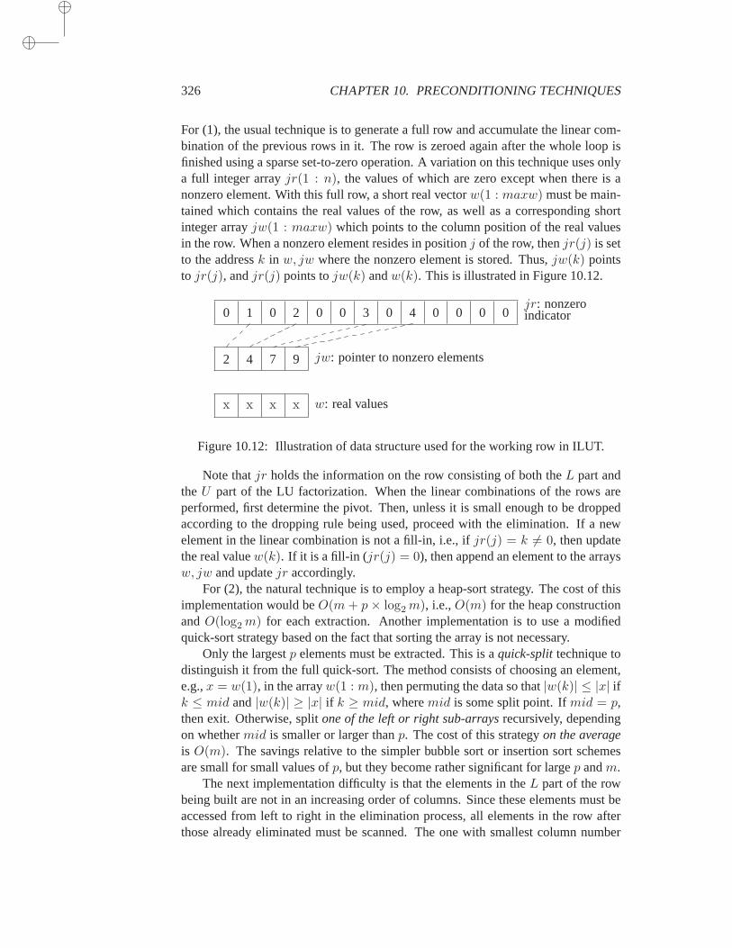
326 CHAPTER 10. PRECONDITIONING TECHNIQUES
For (1), the usual technique is to generate a full row and accumulate the linear com-bination of the previous rows in it. The row is zeroed again after the whole loop isfinished using a sparse set-to-zero operation. A variation on this technique uses onlya full integer arrayjr(1 : n), the values of which are zero except when there is anonzero element. With this full row, a short real vectorw(1 : maxw) must be main-tained which contains the real values of the row, as well as a corresponding shortinteger arrayjw(1 : maxw) which points to the column position of the real valuesin the row. When a nonzero element resides in positionj of the row, thenjr(j) is setto the addressk in w, jw where the nonzero element is stored. Thus,jw(k) pointsto jr(j), andjr(j) points tojw(k) andw(k). This is illustrated in Figure 10.12.
1
2
0 0 2
4
0 0 3
7
0 4
9
0 0 0 0
x x x x w: real values
jw: pointer to nonzero elements
jr: nonzeroindicator
Figure 10.12: Illustration of data structure used for the working row in ILUT.
Note thatjr holds the information on the row consisting of both theL part andtheU part of the LU factorization. When the linear combinations of the rows areperformed, first determine the pivot. Then, unless it is small enough to be droppedaccording to the dropping rule being used, proceed with the elimination. If a newelement in the linear combination is not a fill-in, i.e., ifjr(j) = k 6= 0, then updatethe real valuew(k). If it is a fill-in ( jr(j) = 0), then append an element to the arraysw, jw and updatejr accordingly.
For (2), the natural technique is to employ a heap-sort strategy. The cost of thisimplementation would beO(m+ p× log2m), i.e.,O(m) for the heap constructionandO(log2m) for each extraction. Another implementation is to use a modifiedquick-sort strategy based on the fact that sorting the array is not necessary.
Only the largestp elements must be extracted. This is aquick-splittechnique todistinguish it from the full quick-sort. The method consists of choosing an element,e.g.,x = w(1), in the arrayw(1 : m), then permuting the data so that|w(k)| ≤ |x| ifk ≤ mid and|w(k)| ≥ |x| if k ≥ mid, wheremid is some split point. Ifmid = p,then exit. Otherwise, splitone of the left or right sub-arraysrecursively, dependingon whethermid is smaller or larger thanp. The cost of this strategyon the averageis O(m). The savings relative to the simpler bubble sort or insertion sort schemesare small for small values ofp, but they become rather significant for largep andm.
The next implementation difficulty is that the elements in theL part of the rowbeing built are not in an increasing order of columns. Since these elements must beaccessed from left to right in the elimination process, all elements in the row afterthose already eliminated must be scanned. The one with smallest column number
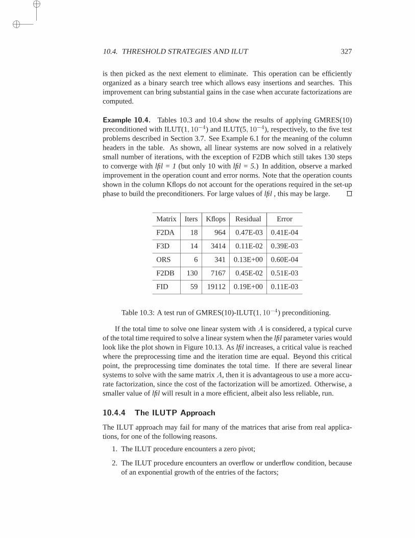
10.4. THRESHOLD STRATEGIES AND ILUT 327
is then picked as the next element to eliminate. This operation can be efficientlyorganized as a binary search tree which allows easy insertions and searches. Thisimprovement can bring substantial gains in the case when accurate factorizations arecomputed.
Example 10.4. Tables 10.3 and 10.4 show the results of applying GMRES(10)preconditioned with ILUT(1, 10−4) and ILUT(5, 10−4), respectively, to the five testproblems described in Section 3.7. See Example 6.1 for the meaning of the columnheaders in the table. As shown, all linear systems are now solved in a relativelysmall number of iterations, with the exception of F2DB which still takes 130 stepsto converge withlfil = 1 (but only 10 withlfil = 5. ) In addition, observe a markedimprovement in the operation count and error norms. Note that the operationcountsshown in the column Kflops do not account for the operations required in the set-upphase to build the preconditioners. For large values oflfil , this may be large.
Matrix Iters Kflops Residual Error
F2DA 18 964 0.47E-03 0.41E-04
F3D 14 3414 0.11E-02 0.39E-03
ORS 6 341 0.13E+00 0.60E-04
F2DB 130 7167 0.45E-02 0.51E-03
FID 59 19112 0.19E+00 0.11E-03
Table 10.3: A test run of GMRES(10)-ILUT(1, 10−4) preconditioning.
If the total time to solve one linear system withA is considered, a typical curveof the total time required to solve a linear system when thelfil parameter varies wouldlook like the plot shown in Figure 10.13. Aslfil increases, a critical value is reachedwhere the preprocessing time and the iteration time are equal. Beyond this criticalpoint, the preprocessing time dominates the total time. If there are several linearsystems to solve with the same matrixA, then it is advantageous to use a more accu-rate factorization, since the cost of the factorization will be amortized. Otherwise, asmaller value oflfil will result in a more efficient, albeit also less reliable, run.
10.4.4 The ILUTP Approach
The ILUT approach may fail for many of the matrices that arise from real applica-tions, for one of the following reasons.
1. The ILUT procedure encounters a zero pivot;
2. The ILUT procedure encounters an overflow or underflow condition, becauseof an exponential growth of the entries of the factors;
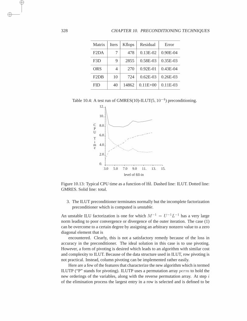
328 CHAPTER 10. PRECONDITIONING TECHNIQUES
Matrix Iters Kflops Residual Error
F2DA 7 478 0.13E-02 0.90E-04
F3D 9 2855 0.58E-03 0.35E-03
ORS 4 270 0.92E-01 0.43E-04
F2DB 10 724 0.62E-03 0.26E-03
FID 40 14862 0.11E+00 0.11E-03
Table 10.4: A test run of GMRES(10)-ILUT(5, 10−4) preconditioning.
level of fill-in
CPU
Time
3.0 5.0 7.0 9.0 11. 13. 15.0.
2.0
4.0
6.0
8.0
10.
12.
Figure 10.13: Typical CPU time as a function of lfil. Dashed line: ILUT. Dottedline:GMRES. Solid line: total.
3. The ILUT preconditioner terminates normally but the incomplete factorizationpreconditioner which is computed isunstable.
An unstable ILU factorization is one for whichM−1 = U−1L−1 has a very largenorm leading to poor convergence or divergence of the outer iteration.The case (1)can be overcome to a certain degree by assigning an arbitrary nonzero value to a zerodiagonal element that is
encountered. Clearly, this is not a satisfactory remedy because of the loss inaccuracy in the preconditioner. The ideal solution in this case is to use pivoting.However, a form of pivoting is desired which leads to an algorithm with similar costand complexity to ILUT. Because of the data structure used in ILUT, row pivoting isnot practical. Instead, column pivoting can be implemented rather easily.
Here are a few of the features that characterize the new algorithm which istermedILUTP (“P” stands for pivoting). ILUTP uses a permutation arrayperm to hold thenew orderings of the variables, along with the reverse permutation array.At stepiof the elimination process the largest entry in a row is selected and is defined tobe
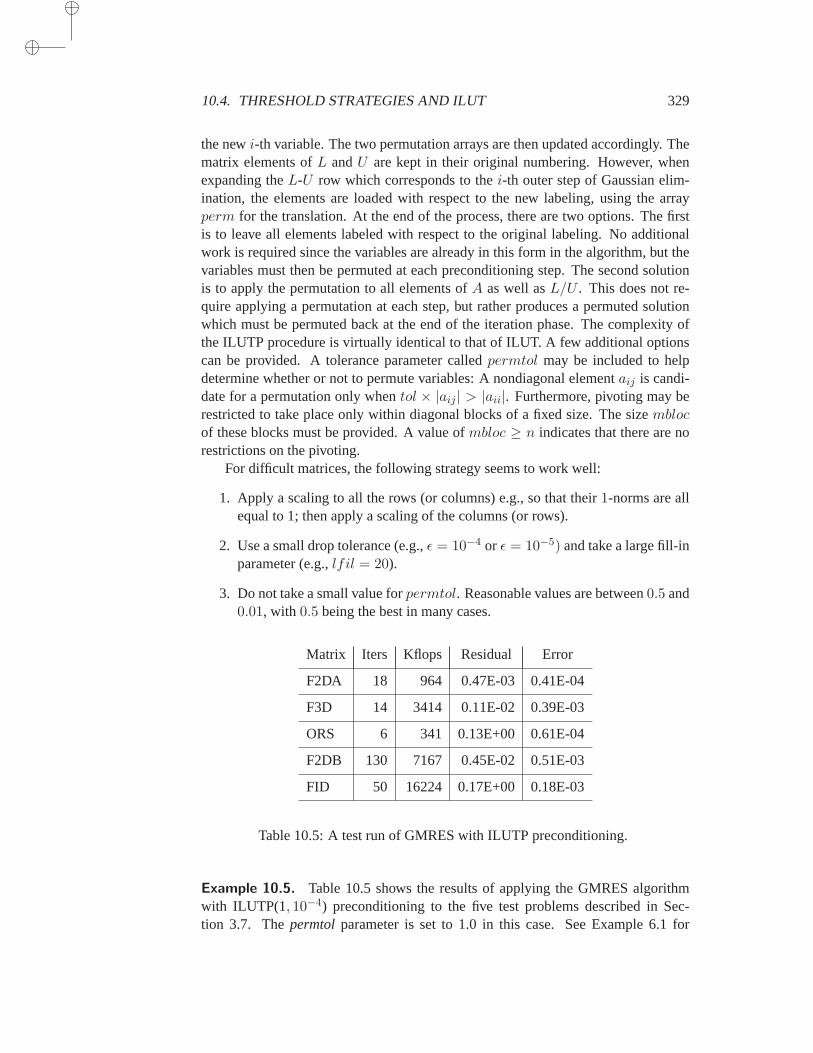
10.4. THRESHOLD STRATEGIES AND ILUT 329
the newi-th variable. The two permutation arrays are then updated accordingly. Thematrix elements ofL andU are kept in their original numbering. However, whenexpanding theL-U row which corresponds to thei-th outer step of Gaussian elim-ination, the elements are loaded with respect to the new labeling, using the arrayperm for the translation. At the end of the process, there are two options. The firstis to leave all elements labeled with respect to the original labeling. No additionalwork is required since the variables are already in this form in the algorithm, but thevariables must then be permuted at each preconditioning step. The secondsolutionis to apply the permutation to all elements ofA as well asL/U . This does not re-quire applying a permutation at each step, but rather produces a permutedsolutionwhich must be permuted back at the end of the iteration phase. The complexity ofthe ILUTP procedure is virtually identical to that of ILUT. A few additional optionscan be provided. A tolerance parameter calledpermtol may be included to helpdetermine whether or not to permute variables: A nondiagonal elementaij is candi-date for a permutation only whentol × |aij | > |aii|. Furthermore, pivoting may berestricted to take place only within diagonal blocks of a fixed size. The sizemblocof these blocks must be provided. A value ofmbloc ≥ n indicates that there are norestrictions on the pivoting.
For difficult matrices, the following strategy seems to work well:
1. Apply a scaling to all the rows (or columns) e.g., so that their1-norms are allequal to 1; then apply a scaling of the columns (or rows).
2. Use a small drop tolerance (e.g.,ǫ = 10−4 or ǫ = 10−5) and take a large fill-inparameter (e.g.,lfil = 20).
3. Do not take a small value forpermtol. Reasonable values are between0.5 and0.01, with 0.5 being the best in many cases.
Matrix Iters Kflops Residual Error
F2DA 18 964 0.47E-03 0.41E-04
F3D 14 3414 0.11E-02 0.39E-03
ORS 6 341 0.13E+00 0.61E-04
F2DB 130 7167 0.45E-02 0.51E-03
FID 50 16224 0.17E+00 0.18E-03
Table 10.5: A test run of GMRES with ILUTP preconditioning.
Example 10.5. Table 10.5 shows the results of applying the GMRES algorithmwith ILUTP(1, 10−4) preconditioning to the five test problems described in Sec-tion 3.7. Thepermtol parameter is set to 1.0 in this case. See Example 6.1 for
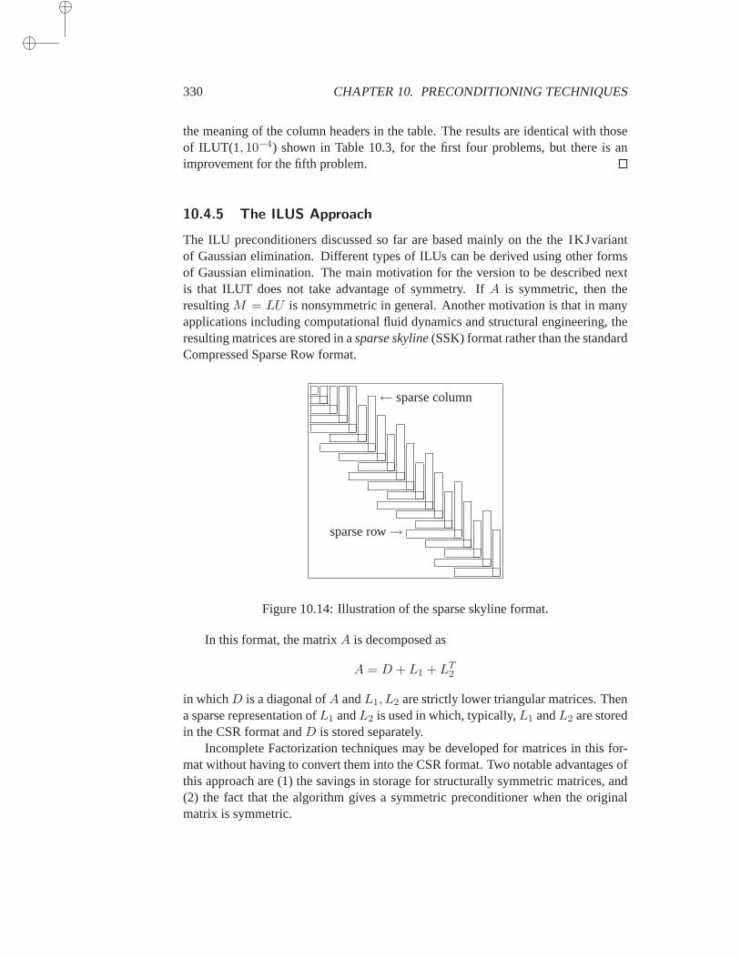
330 CHAPTER 10. PRECONDITIONING TECHNIQUES
the meaning of the column headers in the table. The results are identical with thoseof ILUT(1, 10−4) shown in Table 10.3, for the first four problems, but there is animprovement for the fifth problem.
10.4.5 The ILUS Approach
The ILU preconditioners discussed so far are based mainly on the the IKJvariantof Gaussian elimination. Different types of ILUs can be derived using other formsof Gaussian elimination. The main motivation for the version to be described nextis that ILUT does not take advantage of symmetry. IfA is symmetric, then theresultingM = LU is nonsymmetric in general. Another motivation is that in manyapplications including computational fluid dynamics and structural engineering, theresulting matrices are stored in asparse skyline(SSK) format rather than the standardCompressed Sparse Row format.
sparse row→
← sparse column
Figure 10.14: Illustration of the sparse skyline format.
In this format, the matrixA is decomposed as
A = D + L1 + LT2
in whichD is a diagonal ofA andL1, L2 are strictly lower triangular matrices. Thena sparse representation ofL1 andL2 is used in which, typically,L1 andL2 are storedin the CSR format andD is stored separately.
Incomplete Factorization techniques may be developed for matrices in this for-mat without having to convert them into the CSR format. Two notable advantages ofthis approach are (1) the savings in storage for structurally symmetric matrices, and(2) the fact that the algorithm gives a symmetric preconditioner when the originalmatrix is symmetric.
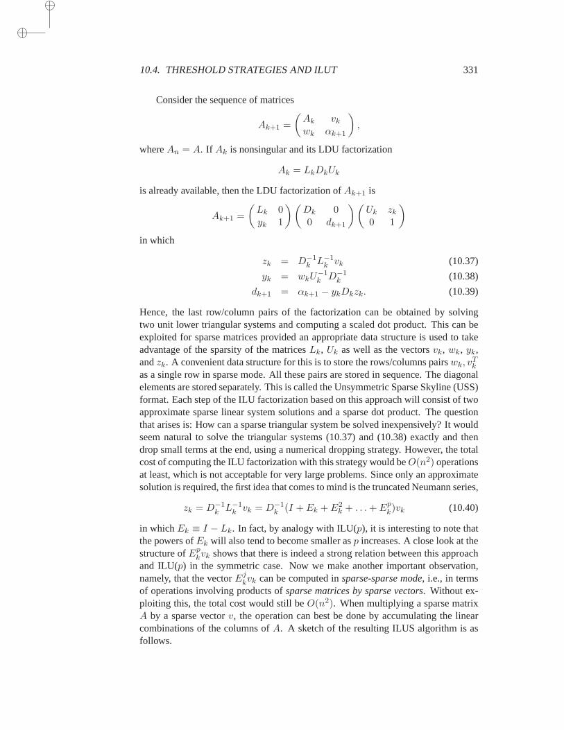
10.4. THRESHOLD STRATEGIES AND ILUT 331
Consider the sequence of matrices
Ak+1 =
(Ak vk
wk αk+1
)
,
whereAn = A. If Ak is nonsingular and its LDU factorization
Ak = LkDkUk
is already available, then the LDU factorization ofAk+1 is
Ak+1 =
(Lk 0yk 1
)(Dk 00 dk+1
)(Uk zk0 1
)
in which
zk = D−1k L−1
k vk (10.37)
yk = wkU−1k D−1
k (10.38)
dk+1 = αk+1 − ykDkzk. (10.39)
Hence, the last row/column pairs of the factorization can be obtained by solvingtwo unit lower triangular systems and computing a scaled dot product. This can beexploited for sparse matrices provided an appropriate data structure is used to takeadvantage of the sparsity of the matricesLk, Uk as well as the vectorsvk, wk, yk,andzk. A convenient data structure for this is to store the rows/columns pairswk, v
Tk
as a single row in sparse mode. All these pairs are stored in sequence. The diagonalelements are stored separately. This is called the Unsymmetric Sparse Skyline (USS)format. Each step of the ILU factorization based on this approach will consist of twoapproximate sparse linear system solutions and a sparse dot product. The questionthat arises is: How can a sparse triangular system be solved inexpensively? It wouldseem natural to solve the triangular systems (10.37) and (10.38) exactly and thendrop small terms at the end, using a numerical dropping strategy. However, the totalcost of computing the ILU factorization with this strategy would beO(n2) operationsat least, which is not acceptable for very large problems. Since only an approximatesolution is required, the first idea that comes to mind is the truncated Neumann series,
zk = D−1k L−1
k vk = D−1k (I + Ek + E2
k + . . .+ Epk)vk (10.40)
in whichEk ≡ I − Lk. In fact, by analogy with ILU(p), it is interesting to note thatthe powers ofEk will also tend to become smaller asp increases. A close look at thestructure ofEp
kvk shows that there is indeed a strong relation between this approachand ILU(p) in the symmetric case. Now we make another important observation,namely, that the vectorEj
kvk can be computed insparse-sparse mode, i.e., in termsof operations involving products ofsparse matrices by sparse vectors. Without ex-ploiting this, the total cost would still beO(n2). When multiplying a sparse matrixA by a sparse vectorv, the operation can best be done by accumulating the linearcombinations of the columns ofA. A sketch of the resulting ILUS algorithm is asfollows.

332 CHAPTER 10. PRECONDITIONING TECHNIQUES
ALGORITHM 10.7 ILUS(ǫ, p)
1. SetA1 = D1 = a11, L1 = U1 = 12. Fori = 1, . . . , n− 1 Do:3. Computezk by (10.40) in sparse-sparse mode4. Computeyk in a similar way5. Apply numerical dropping toyk andzk6. Computedk+1 via (10.39)7. EndDo
If there are onlyi nonzero components in the vectorv and an average ofν nonzeroelements per column, then the total cost per step will be2 × i × ν on the average.Note that the computation ofdk via (10.39) involves the inner product of two sparsevectors which is often implemented by expanding one of the vectors into a full vectorand computing the inner product of a sparse vector by this full vector. Asmentionedbefore, in the symmetric case ILUS yields the Incomplete Cholesky factorization.Here, the work can be halved since the generation ofyk is not necessary.
Also note that a simple iterative procedure such as MR or GMRES(m) can beused to solve the triangular systems in sparse-sparse mode. Similar techniques willbe seen in Section 10.5. Experience shows that these alternatives are not much betterthan the Neumann series approach [79].
10.4.6 The Crout ILU Approach
A notable disadvantage of the standard delayed-updateIKJ factorization is thatit requires access to the entries in thek-th row of L in sorted order of columns.This is further complicated by the fact that the working row (denoted byw in Algo-rithm 10.6), is dynamically modified by fill-in as the elimination proceeds. Searchingfor the leftmost entry in thek-th row ofL is usually not a problem when the fill-inallowed is small. Otherwise, when an accurate factorization is sought, it can becomea significant burden and may ultimately even dominate the cost of the factorization.Sparse direct solution methods that are based on the IKJ form of Gaussian elimina-tion obviate this difficulty by a technique known as the Gilbert-Peierls method [146].Because of dropping, this technique cannot, however, be used as is. Another possibleoption is to reduce the cost of the searches through the use of clever datastructuresand algorithms, such as binary search trees or heaps [90].
The Crout formulation provides the most elegant solution to the problem. In factthe Crout version of Gaussian elimination has other advantages which make itone ofthe most appealing ways of implementing incomplete LU factorizations.
The Crout form of Gaussian elimination consists of computing, at stepk, theentriesak+1:n,k (in the unit lower triangular factor,L) andak,k:n (in the upper trian-gular factor,U ). This is done by post-poning the rank-one update in a way similarto the IKJ variant. In Figure 10.15 the parts of the factors being computed atthek-th step are shown in black and those being accessed are in the shaded areas. At thek-th step, all the updates of the previous steps are applied to the entriesak+1:n,k andak,k:n and it is therefore convenient to storeL by columns andU by rows.
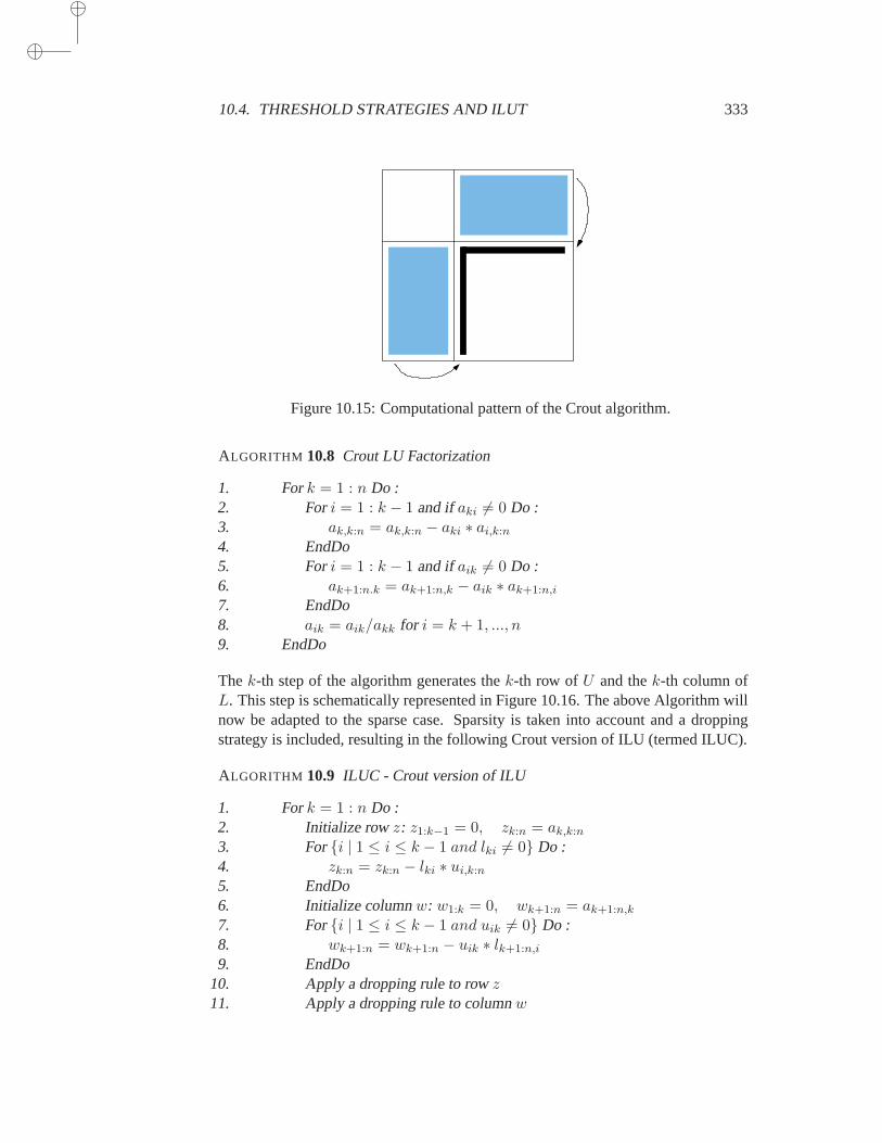
10.4. THRESHOLD STRATEGIES AND ILUT 333
Figure 10.15: Computational pattern of the Crout algorithm.
ALGORITHM 10.8 Crout LU Factorization
1. Fork = 1 : n Do :2. Fori = 1 : k − 1 and ifaki 6= 0 Do :3. ak,k:n = ak,k:n − aki ∗ ai,k:n
4. EndDo5. Fori = 1 : k − 1 and ifaik 6= 0 Do :6. ak+1:n.k = ak+1:n,k − aik ∗ ak+1:n,i
7. EndDo8. aik = aik/akk for i = k + 1, ..., n9. EndDo
Thek-th step of the algorithm generates thek-th row ofU and thek-th column ofL. This step is schematically represented in Figure 10.16. The above Algorithmwillnow be adapted to the sparse case. Sparsity is taken into account and a droppingstrategy is included, resulting in the following Crout version of ILU (termed ILUC).
ALGORITHM 10.9 ILUC - Crout version of ILU
1. Fork = 1 : n Do :2. Initialize rowz: z1:k−1 = 0, zk:n = ak,k:n
3. Fori | 1 ≤ i ≤ k − 1 and lki 6= 0 Do :4. zk:n = zk:n − lki ∗ ui,k:n
5. EndDo6. Initialize columnw: w1:k = 0, wk+1:n = ak+1:n,k
7. Fori | 1 ≤ i ≤ k − 1 and uik 6= 0 Do :8. wk+1:n = wk+1:n − uik ∗ lk+1:n,i
9. EndDo10. Apply a dropping rule to rowz11. Apply a dropping rule to columnw
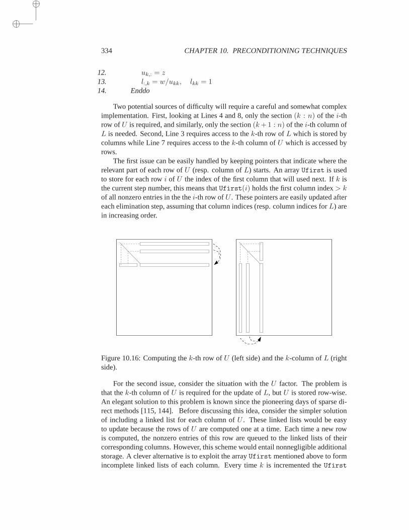
334 CHAPTER 10. PRECONDITIONING TECHNIQUES
12. uk,: = z13. l:,k = w/ukk, lkk = 114. Enddo
Two potential sources of difficulty will require a careful and somewhat compleximplementation. First, looking at Lines 4 and 8, only the section(k : n) of the i-throw ofU is required, and similarly, only the section(k+1 : n) of thei-th column ofL is needed. Second, Line 3 requires access to thek-th row ofL which is stored bycolumns while Line 7 requires access to thek-th column ofU which is accessed byrows.
The first issue can be easily handled by keeping pointers that indicate where therelevant part of each row ofU (resp. column ofL) starts. An arrayUfirst is usedto store for each rowi of U the index of the first column that will used next. Ifk isthe current step number, this means thatUfirst(i) holds the first column index> kof all nonzero entries in the thei-th row ofU . These pointers are easily updated aftereach elimination step, assuming that column indices (resp. column indices forL) arein increasing order.
Figure 10.16: Computing thek-th row ofU (left side) and thek-column ofL (rightside).
For the second issue, consider the situation with theU factor. The problem isthat thek-th column ofU is required for the update ofL, butU is stored row-wise.An elegant solution to this problem is known since the pioneering days of sparse di-rect methods [115, 144]. Before discussing this idea, consider the simpler solutionof including a linked list for each column ofU . These linked lists would be easyto update because the rows ofU are computed one at a time. Each time a new rowis computed, the nonzero entries of this row are queued to the linked lists of theircorresponding columns. However, this scheme would entail nonnegligible additionalstorage. A clever alternative is to exploit the arrayUfirst mentioned above to formincomplete linked lists of each column. Every timek is incremented theUfirst
10.4. THRESHOLD STRATEGIES AND ILUT 335
array is updated. WhenUfirst(i) is updated to point to a new nonzero with columnindexj, then the row indexi is added to the linked list for columni. What is interest-ing is that though the columns structures constructed in this manner are incomplete,they become complete as soon as they are needed.A similar technique is used forthe rows of theL factor.
In addition to avoiding searches, the Crout version of ILU has another importantadvantage. It enables some new dropping strategies which may be viewed as morerigorous than the standard ones seen so far. The straightforward dropping rules usedin ILUT can be easily adapted for ILUC. In addition, the data structure of ILUCallows options which are based on estimating the norms of the inverses ofL andU .
For ILU preconditioners, the error made in the inverses of the factors is moreimportant to control than the errors in the factors themselves. This is because whenA = LU , and
L−1 = L−1 +X U−1 = U−1 + Y,
then the preconditioned matrix is given by
L−1AU−1 = (L−1 +X)A(U−1 + Y ) = I +AY +XA+XY.
If the errorsX andY in the inverses ofL andU are small, then the preconditionedmatrix will be close to the identity matrix. On the other hand, small errors in thefactors themselves may yield arbitrarily large errors in the preconditioned matrix.
Let Lk denote the matrix composed of the firstk rows ofL and the lastn − krows of the identity matrix. Consider a termljk with j > k that is dropped at stepk. Then, the resulting perturbed matrixLk differs fromLk by ljkejeTk . Noticing thatLkej = ej then,
Lk = Lk − ljkejeTk = Lk(I − ljkejeTk )
from which this relation between the inverses follows:
L−1k = (I − ljkejeTk )−1L−1
k = L−1k + ljkeje
TkL
−1k .
Therefore, the inverse ofLk will be perturbed byljk times thek-th row ofL−1k . This
perturbation will affect thej-th row ofL−1k . Hence, using the infinity norm for exam-
ple, it is important to limit the norm of this perturbing row which is‖ljkejeTkL−1k ‖∞.
It follows that it is a good strategy to drop a term inL when
|ljk| ‖eTkL−1k ‖∞ < ǫ.
A similar criterion can be used for the upper triangular factorU .This strategy is not complete because the matrixL−1 is not available. However,
standard techniques used for estimating condition numbers [149] can be adapted forestimating the norm of thek-th row ofL−1 (resp. k-th column ofU−1). The ideais to construct a vectorb one component at a time, by following a greedy strategyto makeL−1b large at each step. This is possible because the firstk − 1 columnsof L are available at thek-th step. The simplest method constructs a vectorb ofcomponentsβk = ±1 at each stepk, in such a way as to maximize the norm of the
336 CHAPTER 10. PRECONDITIONING TECHNIQUES
k-th component ofL−1b. Since the firstk − 1 columns ofL are available at stepk,thek-th component of the solutionx is given by
ξk = βk − eTkLk−1xk−1 .
This makes the choice clear: ifξk is to be large in modulus, then the sign ofβk shouldbe opposite that ofeTkLk−1xk−1. If b is the current right-hand side at stepk, then‖eTkL−1‖∞ can be estimated by thek-th component of the solutionx of the systemLx = b:
‖eTkL−1‖∞ ≈|eTkL−1b|‖b‖∞
.
Details, along with other strategies for dynamically buildingb, may be found in[202].
10.5 Approximate Inverse Preconditioners
The Incomplete LU factorization techniques were developed originally forM -matriceswhich arise from the discretization of Partial Differential Equations of elliptictype,usually in one variable. For the common situation whereA is indefinite, standard ILUfactorizations may face several difficulties, and the best known is the fatal breakdowndue to the encounter of a zero pivot. However, there are other problemsthat are justas serious. Consider an incomplete factorization of the form
A = LU + E (10.41)
whereE is the error. The preconditioned matrices associated with the different formsof preconditioning are similar to
L−1AU−1 = I + L−1EU−1. (10.42)
What is sometimes missed is the fact that the error matrixE in (10.41) is not asimportant as the “preconditioned” error matrixL−1EU−1 shown in (10.42) above.When the matrixA is diagonally dominant, thenL andU are well conditioned, andthe size ofL−1EU−1 remains confined within reasonable limits, typically with anice clustering of its eigenvalues around the origin. On the other hand, when theoriginal matrix is not diagonally dominant,L−1 orU−1 may have very large norms,causing the errorL−1EU−1 to be very large and thus adding large perturbations tothe identity matrix. It can be observed experimentally that ILU preconditioners canbe very poor in these situations which often arise when the matrices are indefinite, orhave large nonsymmetric parts.
One possible remedy is to try to find a preconditioner that does not require solv-ing a linear system. For example, the original system can be preconditioned by amatrixM which is a direct approximation to the inverse ofA.

10.5. APPROXIMATE INVERSE PRECONDITIONERS 337
10.5.1 Approximating the Inverse of a Sparse Matrix
A simple technique for finding approximate inverses of arbitrary sparse matrices isto attempt to find a sparse matrixM which minimizes the Frobenius norm of theresidual matrixI −AM ,
F (M) = ‖I −AM‖2F . (10.43)
A matrixM whose valueF (M) is small would be a right-approximate inverse ofA.Similarly, a left-approximate inverse can be defined by using the objective function
‖I −MA‖2F . (10.44)
Finally, a left-right pairL,U can be sought to minimize
‖I − LAU‖2F . (10.45)
In the following, only (10.43) and(10.45) are considered. The case (10.44) isvery similar to the right preconditioner case (10.43). The objective function (10.43)decouples into the sum of the squares of the 2-norms of the individual columns ofthe residual matrixI −AM ,
F (M) = ‖I −AM‖2F =n∑
j=1
‖ej −Amj‖22 (10.46)
in whichej andmj are thej-th columns of the identity matrix and of the matrixM ,respectively. There are two different ways to proceed in order to minimize(10.46).The function (10.43) can be minimized globally as a function of the sparse matrixM , e.g., by a gradient-type method. Alternatively, the individual functions
fj(m) = ‖ej −Am‖22, j = 1, 2, . . . , n (10.47)
can be minimized. The second approach is appealing for parallel computers, al-though there is also parallelism to be exploited in the first approach. These twoapproaches will be discussed in turn.
10.5.2 Global Iteration
The global iterationapproach consists of treatingM as an unknown sparse matrixand using a descent-type method to minimize the objective function (10.43). Thisfunction is a quadratic function on the space ofn× n matrices, viewed as objects inR
n2. The proper inner product on the space of matrices, to which the squared norm
(10.46) is associated, is〈X,Y 〉 = tr(Y TX). (10.48)
In the following, anarray representationof ann2 vectorX means then× n matrixwhose column vectors are the successiven-vectors ofX.
In a descent algorithm, a new iterateMnew is defined by taking a step along aselected directionG, i.e.,
Mnew = M + αG
338 CHAPTER 10. PRECONDITIONING TECHNIQUES
in which α is selected to minimize the objective functionF (Mnew). From resultsseen in Chapter 5, minimizing the residual norm is equivalent to imposing the con-dition thatR − αAG be orthogonal toAG with respect to the〈·, ·〉 inner product.Thus, the optimalα is given by
α =〈R,AG〉〈AG,AG〉 =
tr(RTAG)
tr ((AG)TAG). (10.49)
The denominator may be computed as‖AG‖2F . The resulting matrixM will tend tobecome denser after each descent step and it is therefore essential to apply a numer-ical dropping strategy to the resultingM . However, the descent property of the stepis now lost, i.e., it is no longer guaranteed thatF (Mnew) ≤ F (M). An alternativewould be to apply numerical dropping to the direction of searchG before taking thedescent step. In this case, the amount of fill-in in the matrixM cannot be controlled.
The simplest choice for the descent directionG is to take it to be equal to theresidual matrixR = I − AM , whereM is the new iterate. Except for the nu-merical dropping step, the corresponding descent algorithm is nothing but the Min-imal Residual (MR) algorithm, seen in Section 5.3.2, on then2 × n2 linear systemAM = I. The global Minimal Residual algorithm will have the following form.
ALGORITHM 10.10 Global Minimal Residual Descent Algorithm
1. Select an initialM2. Until convergence Do:3. ComputeC := AM andG := I − C4. Computeα = tr(GTAG)/‖AG‖2F5. ComputeM := M + αG6. Apply numerical dropping toM7. EndDo
A second choice is to takeG to be equal to the direction of steepest descent, i.e.,the direction opposite to the gradient of the function (10.43) with respect toM . Ifall vectors as represented as 2-dimensionaln × n arrays, then the gradient can beviewed as a matrixG, which satisfies the following relation for small perturbationsE,
F (M + E) = F (M) + 〈G,E〉+ o(‖E‖). (10.50)
This provides a way of expressing the gradient as an operator on arrays, rather thann2 vectors.
Proposition 10.9 The array representation of the gradient ofF with respect toM isthe matrix
G = −2ATR
in whichR is the residual matrixR = I −AM .
10.5. APPROXIMATE INVERSE PRECONDITIONERS 339
Proof. For any matrixE we have
F (M + E)− F (M) = tr[(I −A(M + E))T (I −A(M + E))
]
−tr[(I −AM)T (I −AM)
]
= tr[(R−AE)T (R−AE)−RTR
]
= −tr[(AE)TR+RTAE − (AE)T (AE)
]
= −2tr(RTAE) + tr[(AE)T (AE)
]
= −2⟨ATR,E
⟩+ 〈AE,AE〉 .
Comparing this with (10.50) yields the desired result.
Thus, the steepest descent algorithm will consist of replacingG in line 3 ofAlgorithm 10.10 byG = ATR = AT (I − AM). As is expected with steepestdescent techniques, the algorithm can be slow.
ALGORITHM 10.11 Global Steepest Descent Algorithm
1. Select an initialM2. Until convergence Do:3. ComputeR = I −AM , andG := ATR ;4. Computeα = ‖G‖2F /‖AG‖2F5. ComputeM := M + αG6. Apply numerical dropping toM7. EndDo
In either steepest descent or minimal residual, theG matrix must be stored ex-plicitly. The scalars‖AG‖2F andtr(GTAG) needed to obtainα in these algorithmscan be computed from the successive columns ofAG, which can be generated, used,and discarded. As a result, the matrixAG need not be stored.
10.5.3 Column-Oriented Algorithms
Column-oriented algorithms consist of minimizing the individual objective functions(10.47) separately. Each minimization can be performed by taking a sparse initialguess and solving approximately then parallel linear subproblems
Amj = ej , j = 1, 2, . . . , n (10.51)
with a few steps of a nonsymmetric descent-type method, such as MR or GMRES. Ifthese linear systems were solved (approximately) without taking advantage of spar-sity, the cost of constructing the preconditioner would be of ordern2. That is becauseeach of then columns would requireO(n) operations. Such a cost would becomeunacceptable for large linear systems. To avoid this, the iterations must be performedin sparse-sparse mode, a term which was already introduced in Section 10.4.5. Thecolumnmj and the subsequent iterates in the MR algorithm must be stored and op-erated on as sparse vectors. The Arnoldi basis in the GMRES algorithm are now to
340 CHAPTER 10. PRECONDITIONING TECHNIQUES
be kept in sparse format. Inner products and vector updates involve pairs of sparsevectors.
In the following MR algorithm,ni iterations are used to solve (10.51) approxi-mately for each column, giving an approximation to thej-th column of the inverseof A. Each initialmj is taken from the columns of an initial guess,M0.
ALGORITHM 10.12 Approximate Inverse via MR Iteration
1. Start: setM = M0
2. For each columnj = 1, . . . , n Do:3. Definemj = Mej4. Fori = 1, . . . , nj Do:5. rj := ej −Amj
6. αj :=(rj ,Arj)
(Arj ,Arj)
7. mj := mj + αjrj8. Apply numerical dropping tomj
9. EndDo10. EndDo
The algorithm computes the current residualrj and then minimizes the residualnorm‖ej −A(mj + αrj)‖2, with respect toα. The resulting column is then prunedby applying the numerical dropping step in line 8.
In the sparse implementation of MR and GMRES, the matrix-vector product,SAXPY, and dot product kernels now all involve sparse vectors. Thematrix-vectorproduct is much more efficient if the sparse matrix is stored by columns, sinceallthe entries do not need to be traversed. Efficient codes for all these kernels may beconstructed which utilize a fulln-length work vector.
Columns from an initial guessM0 for the approximate inverse are used as theinitial guesses for the iterative solution of the linear subproblems. There are two ob-vious choices:M0 = αI andM0 = αAT . The scale factorα is chosen to minimizethe norm ofI − AM0. Thus, the initial guess is of the formM0 = αG whereG iseither the identity orAT . The optimalα can be computed using the formula (10.49),in whichR is to be replaced by the identity, soα = tr(AG)/tr(AG(AG)T ). Theidentity initial guess is less expensive to use butM0 = αAT is sometimes a muchbetter initial guess. For this choice, the initial preconditioned systemAM0 is SPD.
The linear systems needed to solve when generating each column of the approx-imate inverse may themselves be preconditioned with the most recent version ofthepreconditioning matrixM . Thus, each system (10.51) for approximating columnjmay be preconditioned withM ′
0 where the firstj − 1 columns ofM ′0 are themk that
already have been computed,1 ≤ k < j, and the remaining columns are the initialguesses for themk, j ≤ k ≤ n. Thus,outer iterations can be defined which sweepover the matrix, as well asinner iterations which compute each column. At eachouter iteration, the initial guess for each column is taken to be the previous result forthat column.
10.5. APPROXIMATE INVERSE PRECONDITIONERS 341
10.5.4 Theoretical Considerations
The first theoretical question which arises is whether or not the approximate inversesobtained by the approximations described earlier can be singular. It cannot be provedthatM is nonsingular unless the approximation is accurate enough. This requirementmay be in conflict with the requirement of keeping the approximation sparse.
Proposition 10.10 Assume thatA is nonsingular and that the residual of the ap-proximate inverseM satisfies the relation
‖I −AM‖ < 1 (10.52)
where‖.‖ is any consistent matrix norm. ThenM is nonsingular.
Proof. The result follows immediately from the equality
AM = I − (I −AM) ≡ I −N. (10.53)
Since‖N‖ < 1, Theorem 1.11 seen in Chapter 1 implies thatI −N is nonsingular.
The result is true in particular for the Frobenius norm which is consistent (see Chapter1).
It may sometimes be the case thatAM is poorly balanced and as a resultRcan be large. Then balancingAM can yield a smaller norm and possibly a lessrestrictive condition for the nonsingularity ofM . It is easy to extend the previousresult as follows. IfA is nonsingular and two nonsingular diagonal matricesD1, D2
exist such that‖I −D1AMD2‖ < 1 (10.54)
where‖.‖ is any consistent matrix norm, thenM is nonsingular.Each column is obtained independently by requiring a condition on the residual
norm of the form‖ej −Amj‖ ≤ τ, (10.55)
for some vector norm‖.‖. From a practical point of view the 2-norm is preferablesince it is related to the objective function which is used, namely, the Frobenius normof the residualI−AM . However, the 1-norm is of particular interest since it leads toa number of simple theoretical results. In the following, it is assumed that a conditionof the form
‖ej −Amj‖1 ≤ τj (10.56)
is required for each column.The above proposition does not reveal anything about the degree of sparsity of
the resulting approximate inverseM . It may well be the case that in order to guaran-tee nonsingularity,M must be dense, or nearly dense. In fact, in the particular casewhere the norm in the proposition is the 1-norm, it is known that the approximate
342 CHAPTER 10. PRECONDITIONING TECHNIQUES
inverse may bestructurally dense, in that it is always possible to find a sparse matrixA for whichM will be dense if‖I −AM‖1 < 1.
Next, we examine the sparsity ofM and prove a simple result for the case wherean assumption of the form (10.56) is made.
Proposition 10.11 Assume thatM is an approximate inverse ofA computed by en-forcing the condition (10.56). LetB = A−1 and assume that a given elementbij ofB satisfies the inequality
|bij | > τj maxk=1,n
|bik|, (10.57)
then the elementmij is nonzero.
Proof. From the equalityAM = I −R we haveM = A−1 −A−1R, and hence
mij = bij −n∑
k=1
bikrkj .
Therefore,
|mij | ≥ |bij | −n∑
k=1
|bikrkj |
≥ |bij | − maxk=1,n
|bik| ‖rj‖1≥ |bij | − max
k=1,n|bik|τj .
Now the condition (10.57) implies that|mij | > 0.
The proposition implies that ifR is small enough, then the nonzero elements ofMare located in positions corresponding to the larger elements in the inverse ofA. Thefollowing negative result is an immediate corollary.
Corollary 10.12 Assume thatM is an approximate inverse ofA computed by en-forcing the condition (10.56) and letτ = maxj=1,...,n τj . If the nonzero elements ofB = A−1 are τ -equimodular in that
|bij | > τ maxk=1,n, l=1,n
|blk|,
then the nonzero sparsity pattern ofM includes the nonzero sparsity pattern ofA−1.In particular, if A−1 is dense and its elements areτ -equimodular, thenM is alsodense.
The smaller the value ofτ , the more likely the condition of the corollary will be sat-isfied. Another way of stating the corollary is thataccurateandsparseapproximateinverses may be computed only if the elements of the actual inverse have variationsin size. Unfortunately, this is difficult to verify in advance and it is known to be trueonly for certain types of matrices.

10.5. APPROXIMATE INVERSE PRECONDITIONERS 343
10.5.5 Convergence of Self Preconditioned MR
We now examine the convergence of the MR algorithm in the case where self precon-ditioning is used, but no numerical dropping is applied. The column-orientedalgo-rithm is considered first. LetM be the current approximate inverse at a given sub-step. The self preconditioned MR iteration for computing thej-th column of the nextapproximate inverse is obtained by the following sequence of operations:
1. rj := ej −Amj = ej −AMej2. tj := Mrj
3. αj :=(rj ,Atj)(Atj ,Atj)
4. mj := mj + αjtj .
Note thatαj can be written as
αj =(rj , AMrj)
(AMrj , AMrj)≡ (rj , Crj)
(Crj , Crj)
whereC = AM
is the preconditioned matrix at the given substep. The subscriptj is now dropped tosimplify the notation. The new residual associated with the current column is givenby
rnew = r − αAt = r − αAMr ≡ r − αCr.The orthogonality of the new residual againstAMr can be used to obtain
‖rnew‖22 = ‖r‖22 − α2‖Cr‖22.Replacingα by its value defined above we get
‖rnew‖22 = ‖r‖22
[
1−(
(Cr, r)
‖Cr‖2‖r‖2
)2]
.
Thus, at each inner iteration, the residual norm for thej-th column is reduced ac-cording to the formula
‖rnew‖2 = ‖r‖2 sin∠(r, Cr) (10.58)
in which ∠(u, v) denotes the acute angle between the vectorsu andv. Assume thateach column converges. Then, the preconditioned matrixC converges to the identity.As a result of this, the angle∠(r, Cr) will tend to∠(r, r) = 0, and therefore the con-vergence ratiosin ∠(r, Cr) will also tend to zero, showing superlinear convergence.
Now consider equation (10.58) more carefully. Denote byR the residual matrixR = I −AM and observe that
sin∠(r, Cr) = minα
‖r − α Cr‖2‖r‖2
≤ ‖r − Cr‖2‖r‖2
≡ ‖Rr‖2‖r‖2≤ ‖R‖2.
344 CHAPTER 10. PRECONDITIONING TECHNIQUES
This results in the following statement.
Proposition 10.13 Assume that the self preconditioned MR algorithm is employedwith one inner step per iteration and no numerical dropping. Then the 2-norm of eachresidualej −Amj of thej-th column is reduced by a factor of at least‖I −AM‖2,whereM is the approximate inverse before the current step, i.e.,
‖rnewj ‖2 ≤ ‖I −AM‖2 ‖rj‖2. (10.59)
In addition, the residual matricesRk = I−AMk obtained after each outer iterationsatisfy
‖Rk+1‖F ≤ ‖Rk‖2F . (10.60)
As a result, when the algorithm converges, it does so quadratically.
Proof. Inequality (10.59) was proved above. To prove quadratic convergence, firstuse the inequality‖X‖2 ≤ ‖X‖F and (10.59) to obtain
‖rnewj ‖2 ≤ ‖Rk,j‖F ‖rj‖2.
Here, thek index corresponds to the outer iteration and thej-index to the column.Note that the Frobenius norm is reduced for each of the inner steps corresponding tothe columns, and therefore,
‖Rk,j‖F ≤ ‖Rk‖F .
This yields‖rnew
j ‖22 ≤ ‖Rk‖2F ‖rj‖22which, upon summation overj, gives
‖Rk+1‖F ≤ ‖Rk‖2F .
This completes the proof.
Note that the above theorem does not prove convergence. It only states that whenthe algorithm converges, it does so quadratically at the limit. In addition, the resultceases to be valid in the presence of dropping.
Consider now the case of the global iteration. When self preconditioning is in-corporated into the global MR algorithm (Algorithm 10.10), the search directionbecomesZk = MkRk, whereRk is the current residual matrix. Then, the main stepsof the algorithm (without dropping) are as follows.
1. Rk := I −AMk
2. Zk := MkRk
3. αk := 〈Rk,AZk〉〈AZk,AZk〉
4. Mk+1 := Mk + αkZk
10.5. APPROXIMATE INVERSE PRECONDITIONERS 345
At each step the new residual matrixRk+1 satisfies the relation
Rk+1 = I −AMk+1 = I −A(Mk + αkZk) = Rk − αkAZk.
An important observation is thatRk is a polynomial inR0. This is because, from theabove relation,
Rk+1 = Rk−αkAMkRk = Rk−αk(I −Rk)Rk = (1−αk)Rk +αkR2k. (10.61)
Therefore, induction shows thatRk+1 = p2k(R0) wherepj is a polynomial of degreej. Now define the preconditioned matrices,
Bk ≡ AMk = I −Rk. (10.62)
Then, the following recurrence follows from (10.61),
Bk+1 = Bk + αkBk(I −Bk) (10.63)
and shows thatBk+1 is also a polynomial of degree2k in B0. In particular,if theinitial B0 is symmetric, then so are all subsequentBk’s. This is achieved when theinitial M is a multiple ofAT , namely ifM0 = α0A
T .Similar to the column oriented case, when the algorithm converges it does so
quadratically.
Proposition 10.14 Assume that the self preconditioned global MR algorithm is usedwithout dropping. Then, the residual matrices obtained at each iteration satisfy
‖Rk+1‖F ≤ ‖R2k‖F . (10.64)
As a result, when the algorithm converges, then it does so quadratically.
Proof. Define for anyα,
R(α) = (1− α)Rk + αR2k
Recall thatαk achieves the minimum of‖R(α)‖F over allα’s. In particular,
‖Rk+1‖F = minα‖R(α)‖F
≤ ‖R(1)‖F = ‖R2k‖F (10.65)
≤ ‖Rk‖2F .
This proves quadratic convergence at the limit.
For further properties see Exercise 16.
346 CHAPTER 10. PRECONDITIONING TECHNIQUES
10.5.6 Approximate Inverses via bordering
A notable disadvantage of the right or left preconditioning approach method is that itis difficult to assess in advance whether or not the resulting approximate inverseM isnonsingular. An alternative would be to seek a two-sided approximation, i.e.,a pairL, U , with L lower triangular andU upper triangular, which attempts to minimizethe objective function (10.45). The techniques developed in the previoussectionscan be exploited for this purpose.
In the factored approach, two matricesL andU which areunit lower and uppertriangular matrices are sought such that
LAU ≈ D
whereD is some unknown diagonal matrix. WhenD is nonsingular andLAU = D,thenL,U are calledinverse LU factorsof A since in this caseA−1 = UD−1L.Once more, the matrices are built one column or row at a time. Assume as in Section10.4.5 that we have the sequence of matrices
Ak+1 =
(Ak vk
wk αk+1
)
in whichAn ≡ A. If the inverse factorsLk, Uk are available forAk, i.e.,
LkAkUk = Dk,
then the inverse factorsLk+1, Uk+1 for Ak+1 are easily obtained by writing(Lk 0−yk 1
)(Ak vk
wk αk+1
)(Uk −zk0 1
)
=
(Dk 00 δk+1
)
(10.66)
in whichzk, yk, andδk+1 are such that
Akzk = vk (10.67)
ykAk = wk (10.68)
δk+1 = αk+1 − wkzk = αk+1 − ykvk. (10.69)
Note that the formula (10.69) exploits the fact that either the system (10.67) issolvedexactly (middle expression) or the system (10.68) is solved exactly (second expres-sion) or both systems are solved exactly (either expression). In the realistic situationwhere neither of these two systems is solved exactly, then this formula should bereplaced by
δk+1 = αk+1 − wkzk − ykvk + ykAkzk. (10.70)
The last row/column pairs of the approximate factored inverse can be obtained bysolving two sparse systems and computing a few dot products. It is interesting tonote that the only difference with the ILUS factorization seen in Section 10.4.5isthat the coefficient matrices for these systems are not the triangular factors ofAk,but the matrixAk itself.
10.5. APPROXIMATE INVERSE PRECONDITIONERS 347
To obtain an approximate factorization, simply exploit the fact that theAk ma-trices are sparse and then employ iterative solvers in sparse-sparse mode. In thissituation, formula (10.70) should be used forδk+1. The algorithm would be as fol-lows.
ALGORITHM 10.13 Approximate Inverse Factors Algorithm
1. Fork = 1, . . . , n Do:2. Solve (10.67) approximately;3. Solve (10.68) approximately;4. Computeδk+1 = αk+1 − wkzk − ykvk + ykAkzk5. EndDo
A linear system must be solved withAk in line 2 and a linear system withATk in
line 3. This is a good scenario for the Biconjugate Gradient algorithm or its equiva-lent two-sided Lanczos algorithm. In addition, the most current approximateinversefactors can be used to precondition the linear systems to be solved in steps 2 and 3.This was termed “self preconditioning” earlier. All the linear systems in the abovealgorithm can be solved in parallel since they are independent of one another. ThediagonalD can then be obtained at the end of the process.
This approach is particularly suitable in the symmetric case. Since there is onlyone factor, the amount of work is halved. In addition, there is no problem with theexistence in the positive definite case as is shown in the following lemma which statesthatδk+1 is always> 0 whenA is SPD, independently of the accuracy with whichthe system (10.67) is solved.
Lemma 10.15 LetA be SPD. Then, the scalarδk+1 as computed by (10.70) is posi-tive.
Proof. In the symmetric case,wk = vTk . Note thatδk+1 as computed by formula
(10.70) is the(k + 1, k + 1) element of the matrixLk+1Ak+1LTk+1. It is positive
becauseAk+1 is SPD. This is independent of the accuracy for solving the system toobtainzk.
In the general nonsymmetric case, there is no guarantee thatδk+1 will be nonzero,unless the systems (10.67) and (10.68) are solved accurately enough. There is nopractical problem here, sinceδk+1 is computable. The only question remaining isa theoretical one: Canδk+1 be guaranteed to be nonzero if the systems are solvedwith enough accuracy? Intuitively, if the system is solved exactly, then theD matrixmust be nonzero since it is equal to theD matrix of the exact inverse factors in thiscase. The minimal assumption to make is that eachAk is nonsingular. Letδ∗k+1 bethe value that would be obtained if at least one of the systems (10.67) or (10.68) issolved exactly. According to equation (10.69), in this situation this value is given by
δ∗k+1 = αk+1 − wkA−1k vk. (10.71)
348 CHAPTER 10. PRECONDITIONING TECHNIQUES
If Ak+1 is nonsingular, thenδ∗k+1 6= 0. To see this refer to the defining equation(10.66) and compute the productLk+1Ak+1Uk+1 in the general case. Letrk andsk
be the residuals obtained for these linear systems, i.e.,
rk = vk −Akzk, sk = wk − ykAk. (10.72)
Then a little calculation yields
Lk+1Ak+1Uk+1 =
(LkAkUk LkrkskUk δk+1
)
. (10.73)
If one of rk or sk is zero, then it is clear that the termδk+1 in the above relation be-comesδ∗k+1 and it must be nonzero since the matrix on the left-hand side is nonsingu-lar. Incidentally, this relation shows the structure of the last matrixLnAnUn ≡ LAU .The components1 to j − 1 of columnj consist of the vectorLjrj , the components1 to j − 1 of row i make up the vectorskUk, and the diagonal elements are theδi’s.Consider now the expression forδk+1 from (10.70).
δk+1 = αk+1 − wkzk − ykvk + ykAkzk
= αk+1 − wkA−1k (vk − rk)− (wk − sk)A
−1k vk + (vk − rk)A−1
k (wk − sk)
= αk+1 − vkA−1k wk + rkA
−1k sk
= δ∗k+1 + rkA−1k sk.
This perturbation formula is of a second order in the sense that|δk+1 − δ∗k+1| =
O(‖rk‖ ‖sk‖). It guarantees thatδk+1 is nonzero whenever|rkA−1k sk| < |δ∗k+1|.
10.5.7 Factored inverses via orthogonalization: AINV
The approximate inverse technique (AINV) described in [34, 36] computes an ap-proximate factorization of the formW TAZ = D, whereW,Z are unit upper trian-gular matrices, andD is a diagonal. The matricesW andZ can be directly computedby performing an approximate bi-orthogonalization of the Gram-Schmidt type.In-deed, whenA = LDU is the exact LDU factorization ofA, thenW should be equalto the inverse ofL and we should have the equality
W TA = DU
which means thatW TA is upper triangular. This translates into the result that anycolumni ofW is orthogonal to the firsti−1 columns ofA. A procedure to computeW is therefore to make thei-th column ofW orthogonal to the columns1, . . . , i− 1of A by subtracting multiples of the firsti−1 columns ofW . Alternatively, columnsi + 1, . . . , n of W can be made orthogonal to the firsti columns ofA. This willproduce columns that are orthogonal to each of the columns ofA. During this pro-cedure one can drop small entries, or entries outside a certain sparsity pattern. Asimilar process can be applied to obtain the columns ofZ. The resulting incom-plete biorthogonalization process, which is sketched next, produces an approximatefactored inverse.
10.5. APPROXIMATE INVERSE PRECONDITIONERS 349
ALGORITHM 10.14 Right–looking factored AINV
1. Letp = q = (0, . . . , 0) ∈ Rn, Z = [z1, . . . , zn] = In,W = [w1, . . . , wn] = In.
2. Fork = 1, . . . , n3. pk = wT
k Aek, qk = eTkAzk4. Fori = k + 1, . . . , n5. pi =
(wT
i Aek)/pk, qi =
(eTkAzi
)/qk
6. Apply a dropping rule topi, qi7. wi = wi − wkpi, zi = zi − zkqi8. Apply a dropping rule towj,i andzj,i, for j = 1, . . . , i.9. EndDo
10. EndDo11. Choose diagonal entries ofD as the components ofp or q.
The above algorithm constitutes one of two options for computing factored approxi-mate inverses via approximate orthogonalization. An alternative is based on the factthatW TAZ should become approximately diagonal. Instead of orthogonalizingW(resp. Z) with respect to the columns ofA, a bi-orthogonalization process can beapplied to force the columns ofW andZ to be conjugate with respect toA. For thiswe must require thateTkW
TAZej = 0 for all k 6= j, 1 ≤ k, j ≤ i. The result will bea simple change to Algorithm 10.14. Specifically, the second option, which we labelwith a (b), replaces lines (3) and (5) into the following lines:
3a. pk = wTk Azk, qk = wT
k Azk5b. pi =
(wT
i Azk)/pk, qi =
(wT
k Azi)/qk
If no entries are dropped and if an LDU factorization ofA exists, thenW = LT ,Z =U−1. A little induction proof would then show that after stepi, columnsi+1, . . . , nof W are orthogonal to column1, . . . , i of A and likewise columnsi + 1, . . . , n ofZ are orthogonal to rows1, . . . , i of A. Remarkably, the computations ofZ andWcan be performed independently of each other for the original option represented byAlgorithm 10.14.
In the original version of AINV [34, 36], dropping is performed on the vectorswi
andzi only. Dropping entries frompi, qi seems to not yield as good approximations,see [34].
10.5.8 Improving a Preconditioner
After a computed ILU factorization results in an unsatisfactory convergence, it isdifficult to improve it by modifying theL andU factors. One solution would be todiscard this factorization and attempt to recompute a fresh one possibly with morefill-in. Clearly, this may be a wasteful process. A better alternative is to use approx-imate inverse techniques. Assume a (sparse) matrixM is a preconditioner to theoriginal matrixA, so the preconditioned matrix is
C = M−1A.
350 CHAPTER 10. PRECONDITIONING TECHNIQUES
A sparse matrixS is sought to approximate the inverse ofM−1A. This matrix isthen to be used as a preconditioner toM−1A. Unfortunately, the matrixC is usuallydense. However, observe that all that is needed is a matrixS such that
AS ≈M.
Recall that the columns ofA andM are sparse. One approach is to compute aleast-squares approximation in the Frobenius norm sense. This approach was usedalready in Section 10.5.1 whenM is the identity matrix. Then the columns ofS wereobtained by approximately solving the linear systemsAsi ≈ ei. The same idea canbe applied here. Now, the systems
Asi = mi
must be solved instead, wheremi is thei-th column ofM which is sparse. Thus, thecoefficient matrix and the right-hand side are sparse, as before.
10.6 Reordering for ILU
The primary goal of reordering techniques (see Chapter 3) is to reducefill-in duringGaussian elimination. A difficulty with such methods, whether in the context of di-rect or iterative solvers, is that a good ordering for reducing fill-in may lead to factorsof poor numerical quality. For example, very small diagonal entries may be encoun-tered during the process. Two types of permutations are often used to enhance ILUfactorizations. First, fill-reducing symmetric permutations of the type seen in Chap-ter 3 have been advocated. The argument here is that since these permutations arelikely to produce fewer fill-ins, it is likely that the ILU factorizations resulting fromdropping small terms will be more accurate. A second category of reorderings con-sists of only permuting the rows of the matrix (or its columns). These unsymmetricpermutations address the other issue mentioned above, namely avoiding poorpivotsin Gaussian elimination.
10.6.1 Symmetric permutations
The Reverse Cuthill McKee ordering seen in Section 3.3.3 is among the most com-mon techniques used to enhance the effectiveness of ILU factorizations. Recall thatthis reordering is designed to reduce the envelope of a matrix. Other reorderingsthat are geared specifically toward reducing fill-in, such as the minimum degree ormultiple minimum degree orderings, have also been advocated, though resultsre-ported in the literature are mixed. What is clear is that the results will depend ontheaccuracy of the ILU being computed. If ILU(0), or some low-fill, incompletefac-torization is being used, then it is often reported that it is generally not a good ideato reorder the matrix. Among candidate permutations that can be applied, the RCMis the most likely to yield an improvement. As the accuracy of the preconditionerincreases, i.e. as more fill-ins are allowed, then the beneficial effect of reordering
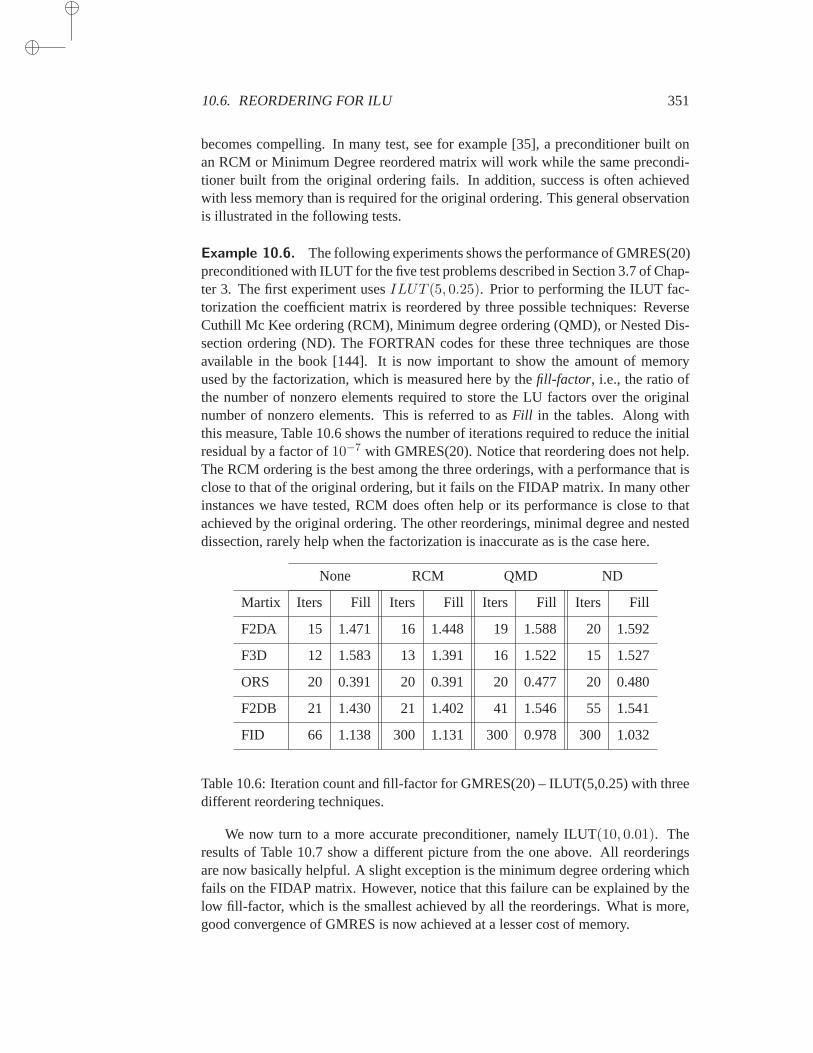
10.6. REORDERING FOR ILU 351
becomes compelling. In many test, see for example [35], a preconditioner built onan RCM or Minimum Degree reordered matrix will work while the same precondi-tioner built from the original ordering fails. In addition, success is often achievedwith less memory than is required for the original ordering. This general observationis illustrated in the following tests.
Example 10.6. The following experiments shows the performance of GMRES(20)preconditioned with ILUT for the five test problems described in Section 3.7 of Chap-ter 3. The first experiment usesILUT (5, 0.25). Prior to performing the ILUT fac-torization the coefficient matrix is reordered by three possible techniques:ReverseCuthill Mc Kee ordering (RCM), Minimum degree ordering (QMD), or Nested Dis-section ordering (ND). The FORTRAN codes for these three techniquesare thoseavailable in the book [144]. It is now important to show the amount of memoryused by the factorization, which is measured here by thefill-factor, i.e., the ratio ofthe number of nonzero elements required to store the LU factors over the originalnumber of nonzero elements. This is referred to asFill in the tables. Along withthis measure, Table 10.6 shows the number of iterations required to reduce the initialresidual by a factor of10−7 with GMRES(20). Notice that reordering does not help.The RCM ordering is the best among the three orderings, with a performance that isclose to that of the original ordering, but it fails on the FIDAP matrix. In manyotherinstances we have tested, RCM does often help or its performance is close tothatachieved by the original ordering. The other reorderings, minimal degree and nesteddissection, rarely help when the factorization is inaccurate as is the case here.
None RCM QMD ND
Martix Iters Fill Iters Fill Iters Fill Iters Fill
F2DA 15 1.471 16 1.448 19 1.588 20 1.592
F3D 12 1.583 13 1.391 16 1.522 15 1.527
ORS 20 0.391 20 0.391 20 0.477 20 0.480
F2DB 21 1.430 21 1.402 41 1.546 55 1.541
FID 66 1.138 300 1.131 300 0.978 300 1.032
Table 10.6: Iteration count and fill-factor for GMRES(20) – ILUT(5,0.25) with threedifferent reordering techniques.
We now turn to a more accurate preconditioner, namely ILUT(10, 0.01). Theresults of Table 10.7 show a different picture from the one above. All reorderingsare now basically helpful. A slight exception is the minimum degree ordering whichfails on the FIDAP matrix. However, notice that this failure can be explained by thelow fill-factor, which is the smallest achieved by all the reorderings. What ismore,good convergence of GMRES is now achieved at a lesser cost of memory.
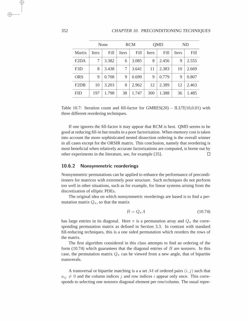
352 CHAPTER 10. PRECONDITIONING TECHNIQUES
None RCM QMD ND
Martix Iters Fill Iters Fill Iters Fill Iters Fill
F2DA 7 3.382 6 3.085 8 2.456 9 2.555
F3D 8 3.438 7 3.641 11 2.383 10 2.669
ORS 9 0.708 9 0.699 9 0.779 9 0.807
F2DB 10 3.203 8 2.962 12 2.389 12 2.463
FID 197 1.798 38 1.747 300 1.388 36 1.485
Table 10.7: Iteration count and fill-factor for GMRES(20) – ILUT(10,0.01) withthree different reordering techniques.
If one ignores the fill-factor it may appear that RCM is best. QMD seems to begood at reducing fill-in but results in a poor factorization. When memory cost is takeninto account the more sophisticated nested dissection ordering is the overallwinnerin all cases except for the ORSIR matrix. This conclusion, namely that reordering ismost beneficial when relatively accurate factorizations are computed, is borne out byother experiments in the literature, see, for example [35].
10.6.2 Nonsymmetric reorderings
Nonsymmetric permutations can be applied to enhance the performance of precondi-tioners for matrices with extremely poor structure. Such techniques do not performtoo well in other situations, such as for example, for linear systems arising from thediscretization of elliptic PDEs.
The original idea on which nonsymmetric reorderings are based is to find a per-mutation matrixQπ, so that the matrix
B = QπA (10.74)
has large entries in its diagonal. Hereπ is a permutation array andQπ the corre-sponding permutation matrix as defined in Section 3.3. In contrast with standardfill-reducing techniques, this is a one sided permutation which reorders the rows ofthe matrix.
The first algorithm considered in this class attempts to find an ordering of theform (10.74) which guarantees that the diagonal entries ofB are nonzero. In thiscase, the permutation matrixQπ can be viewed from a new angle, that of bipartitetransverals.
A transversal or bipartite matching is a a setM of ordered pairs(i, j) such thataij 6= 0 and the column indicesj and row indicesi appear only once. This corre-sponds to selecting one nonzero diagonal element per row/column. The usual repre-
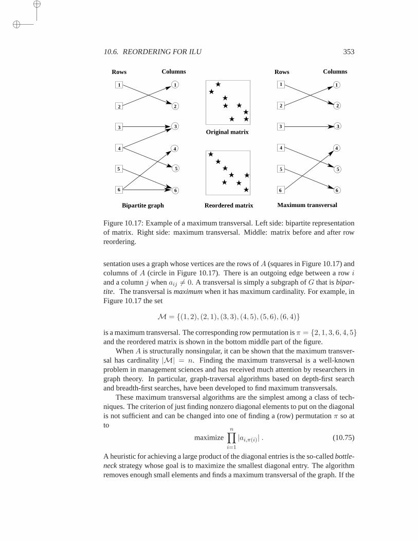
10.6. REORDERING FOR ILU 353
5
3
2
3
4
5
6
2
1
4
5
6
2
4
5
6
1
Reordered matrix Bipartite graph Maximum transversal
ColumnsRowsColumnsRows
Original matrix
1
3 3
2
6
1
4
Figure 10.17: Example of a maximum transversal. Left side: bipartite representationof matrix. Right side: maximum transversal. Middle: matrix before and after rowreordering.
sentation uses a graph whose vertices are the rows ofA (squares in Figure 10.17) andcolumns ofA (circle in Figure 10.17). There is an outgoing edge between a rowiand a columnj whenaij 6= 0. A transversal is simply a subgraph ofG that isbipar-tite. The transversal ismaximumwhen it has maximum cardinality. For example, inFigure 10.17 the set
M = (1, 2), (2, 1), (3, 3), (4, 5), (5, 6), (6, 4)
is a maximum transversal. The corresponding row permutation isπ = 2, 1, 3, 6, 4, 5and the reordered matrix is shown in the bottom middle part of the figure.
WhenA is structurally nonsingular, it can be shown that the maximum transver-sal has cardinality|M| = n. Finding the maximum transversal is a well-knownproblem in management sciences and has received much attention by researchers ingraph theory. In particular, graph-traversal algorithms based on depth-first searchand breadth-first searches, have been developed to find maximum transversals.
These maximum transversal algorithms are the simplest among a class of tech-niques. The criterion of just finding nonzero diagonal elements to put on the diagonalis not sufficient and can be changed into one of finding a (row) permutation π so atto
maximizen∏
i=1
|ai,π(i)| . (10.75)
A heuristic for achieving a large product of the diagonal entries is the so-calledbottle-neckstrategy whose goal is to maximize the smallest diagonal entry. The algorithmremoves enough small elements and finds a maximum transversal of the graph. If the
354 CHAPTER 10. PRECONDITIONING TECHNIQUES
transversal is not of cardinalityn then the algorithm backtracks by removing fewerof the small entries and repeating the process.
Another class of algorithms solve the optimization problem (10.75) more accu-rately. This problem can be translated into
minπ
n∑
i=1
ci,π(i) where cij =
log [ ‖a:,j‖∞ / |aij | ] if aij 6= 0+∞ otherwise
.
It is known that solving this problem is equivalent to solving its dual, which can beformulated as follows:
maxui,uj
n∑
i=1
ui +n∑
j=1
uj
subject to: cij − ui − uj ≥ 0 .
The algorithms used to solve the above dual problem are based on graph theorytechniques - in fact they can be viewed as traversal algorithms (such as depth firstsearch) to which a cost measure is added. Details can be found in [110].
Experiments reported by Duff and Koster [110] and Benzi et al. [32] show thatnonsymmetric reorderings based on the methods discussed in this section canbequite beneficial for those problems which are irregularly structured and have manyzero diagonal entries. On the other hand, they do not perform as well for PDE matri-ces for which symmetric orderings are often superior.
10.7 Block Preconditioners
Block preconditioning is a popular technique for block-tridiagonal matricesarisingfrom the discretization of elliptic problems. It can also be generalized to othersparsematrices. We begin with a discussion of the block-tridiagonal case.
10.7.1 Block-Tridiagonal Matrices
Consider a block-tridiagonal matrix blocked in the form
A =
D1 E2
F2 D2 E3.. . . . . .. .
Fm−1 Dm−1 Em
Fm Dm
. (10.76)
One of the most popular block preconditioners used in the context of PDEsis basedon this block-tridiagonal form of the coefficient matrixA. Let D be the block-diagonal matrix consisting of the diagonal blocksDi,L the block strictly-lower trian-gular matrix consisting of the sub-diagonal blocksFi, andU the block strictly-uppertriangular matrix consisting of the super-diagonal blocksEi. Then, the above matrixhas the form
A = L+D + U.
10.7. BLOCK PRECONDITIONERS 355
A block ILU preconditioner is defined by
M = (L+ ∆)∆−1(∆ + U), (10.77)
whereL andU are the same as above, and∆ is a block-diagonal matrix whose blocks∆i are defined by the recurrence:
∆i = Di − FiΩi−1Ei, (10.78)
in which Ωj is some sparse approximation to∆−1j . Thus, to obtain a block factor-
ization, approximations to the inverses of the blocks∆i must be found. This clearlywill lead to difficulties if explicit inverses are used.
An important particular case is when the diagonal blocksDi of the original ma-trix are tridiagonal, while the co-diagonal blocksEi andFi are diagonal. Then, asimple recurrence formula for computing the inverse of a tridiagonal matrix can beexploited. Only the tridiagonal part of the inverse must be kept in the recurrence(10.78). Thus,
∆1 = D1, (10.79)
∆i = Di − FiΩ(3)i−1Ei, i = 1, . . . ,m, (10.80)
whereΩ(3)k is the tridiagonal part of∆−1
k .
(Ω(3)k )i,j = (∆−1
k )i,j for |i− j| ≤ 1.
The following theorem can be shown.
Theorem 10.16LetA be Symmetric Positive Definite and such that
• aii > 0, i = 1, . . . , n, andaij ≤ 0 for all j 6= i.
• The matricesDi are all (strict) diagonally dominant.
Then each block∆i computed by the recurrence (10.79), (10.80) is a symmetricM -matrix. In particular,M is also a positive definite matrix.
We now show how the inverse of a tridiagonal matrix can be obtained. Let atridiagonal matrix∆ of dimensionl be given in the form
∆ =
α1 −β2
−β2 α2 −β3. . . . .. . ..
−βl−1 αl−1 −βl
−βl αl
,
and let its Cholesky factorization be
∆ = LDLT ,
356 CHAPTER 10. PRECONDITIONING TECHNIQUES
withD = diag δi
and
L =
1−γ2 1
.. . . . .−γl−1 1
−γl 1
.
The inverse of∆ isL−TD−1L−1. Start by observing that the inverse ofLT is a unitupper triangular matrix whose coefficientsuij are given by
uij = γi+1γi+2 . . . γj−1γj for 1 ≤ i < j < l.
As a result, thej-th columncj of L−T is related to the(j− 1)-st columncj−1 by thevery simple recurrence,
cj = ej + γjcj−1, for j ≥ 2
starting with the first columnc1 = e1. The inverse of∆ becomes
∆−1 = L−TD−1L−1 =l∑
j=1
1
δjcjc
Tj . (10.81)
See Exercise 12 for a proof of the above equality. As noted, the recurrence formulasfor computing∆−1 can be unstable and lead to numerical difficulties for large valuesof l.
10.7.2 General Matrices
A general sparse matrix can often be put in the form (10.76) where the blocking iseither natural as provided by the physical problem, or artificial when obtained as aresult of RCMK ordering and some block partitioning. In such cases, a recurrencesuch as (10.78) can still be used to obtain a block factorization defined by (10.77).A 2-level preconditioner can be defined by using sparse inverse approximate tech-niques to approximateΩi. These are sometimes termed implicit-explicit precondi-tioners, the implicit part referring to the block-factorization and the explicit part tothe approximate inverses used to explicitly approximate∆−1
i .
10.8 Preconditioners for the Normal Equations
When the original matrix is strongly indefinite, i.e., when it has eigenvalues spreadon both sides of the imaginary axis, the usual Krylov subspace methods may fail.The Conjugate Gradient approach applied to the normal equations may then becomea good alternative. Choosing to use this alternative over the standard methods may
10.8. PRECONDITIONERS FOR THE NORMAL EQUATIONS 357
involve inspecting the spectrum of a Hessenberg matrix obtained from a smallrun ofan unpreconditioned GMRES algorithm.
If the normal equations approach is chosen, the question becomes how to pre-condition the resulting iteration. An ILU preconditioner can be computed forA andthe preconditioned normal equations,
AT (LU)−T (LU)−1Ax = AT (LU)−T (LU)−1b,
can be solved. However, whenA is not diagonally dominant the ILU factorizationprocess may encounter a zero pivot. Even when this does not happen,the result-ing preconditioner may be of poor quality. An incomplete factorization routine withpivoting, such as ILUTP, may constitute a good choice. ILUTP can be used to pre-condition either the original equations or the normal equations shown above. Thissection explores a few other options available for preconditioning the normal equa-tions.
10.8.1 Jacobi, SOR, and Variants
There are several ways to exploit the relaxation schemes for the Normal Equationsseen in Chapter 8 as preconditioners for the CG method applied to either (8.1)or(8.3). Consider (8.3), for example, which requires a procedure delivering an approx-imation to(AAT )−1v for any vectorv. One such procedure is to perform one stepof SSOR to solve the system(AAT )w = v. Denote byM−1 the linear operator thattransformsv into the vector resulting from this procedure, then the usual ConjugateGradient method applied to (8.3) can be recast in the same form as Algorithm 8.5.This algorithm is known as CGNE/SSOR. Similarly, it is possible to incorporate theSSOR preconditioning in Algorithm 8.4, which is associated with the Normal Equa-tions (8.1), by definingM−1 to be the linear transformation that maps a vectorvinto a vectorw resulting from the forward sweep of Algorithm 8.2 followed by abackward sweep. We will refer to this algorithm as CGNR/SSOR.
The CGNE/SSOR and CGNR/SSOR algorithms will not break down ifA is non-singular, since then the matricesAAT andATA are Symmetric Positive Definite, asare the preconditioning matricesM . There are several variations to these algorithms.The standard alternatives based on the same formulation (8.1) are either to use thepreconditioner on the right, solving the systemATAM−1y = b, or to split the pre-conditioner into a forward SOR sweep on the left and a backward SOR sweep onthe right of the matrixATA. Similar options can also be written for the NormalEquations (8.3) again with three different ways of preconditioning. Thus, at least sixdifferent algorithms can be defined.
10.8.2 IC(0) for the Normal Equations
The Incomplete Cholesky IC(0) factorization can be used to precondition the NormalEquations (8.1) or (8.3). This approach may seem attractive because ofthe successof incomplete factorization preconditioners. However, a major problem is that the
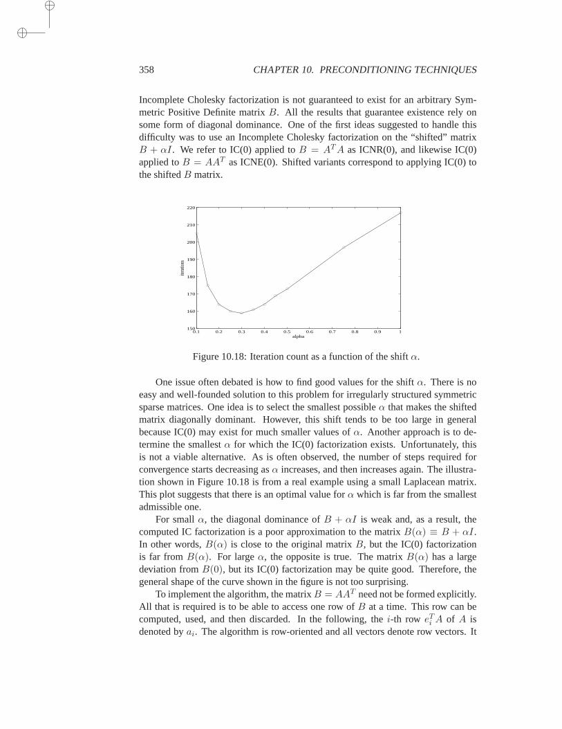
358 CHAPTER 10. PRECONDITIONING TECHNIQUES
Incomplete Cholesky factorization is not guaranteed to exist for an arbitrary Sym-metric Positive Definite matrixB. All the results that guarantee existence rely onsome form of diagonal dominance. One of the first ideas suggested to handle thisdifficulty was to use an Incomplete Cholesky factorization on the “shifted” matrixB + αI. We refer to IC(0) applied toB = ATA as ICNR(0), and likewise IC(0)applied toB = AAT as ICNE(0). Shifted variants correspond to applying IC(0) tothe shiftedB matrix.
0.1 0.2 0.3 0.4 0.5 0.6 0.7 0.8 0.9 1150
160
170
180
190
200
210
220
alpha
itera
tions
Figure 10.18: Iteration count as a function of the shiftα.
One issue often debated is how to find good values for the shiftα. There is noeasy and well-founded solution to this problem for irregularly structured symmetricsparse matrices. One idea is to select the smallest possibleα that makes the shiftedmatrix diagonally dominant. However, this shift tends to be too large in generalbecause IC(0) may exist for much smaller values ofα. Another approach is to de-termine the smallestα for which the IC(0) factorization exists. Unfortunately, thisis not a viable alternative. As is often observed, the number of steps required forconvergence starts decreasing asα increases, and then increases again. The illustra-tion shown in Figure 10.18 is from a real example using a small Laplacean matrix.This plot suggests that there is an optimal value forα which is far from the smallestadmissible one.
For smallα, the diagonal dominance ofB + αI is weak and, as a result, thecomputed IC factorization is a poor approximation to the matrixB(α) ≡ B + αI.In other words,B(α) is close to the original matrixB, but the IC(0) factorizationis far fromB(α). For largeα, the opposite is true. The matrixB(α) has a largedeviation fromB(0), but its IC(0) factorization may be quite good. Therefore, thegeneral shape of the curve shown in the figure is not too surprising.
To implement the algorithm, the matrixB = AAT need not be formed explicitly.All that is required is to be able to access one row ofB at a time. This row can becomputed, used, and then discarded. In the following, thei-th row eTi A of A isdenoted byai. The algorithm is row-oriented and all vectors denote row vectors. It

10.8. PRECONDITIONERS FOR THE NORMAL EQUATIONS 359
is adapted from the ILU(0) factorization of a sparse matrix, i.e., Algorithm 10.4, butit actually computes theLDLT factorization instead of anLU orLLT factorization.The main difference with Algorithm 10.4 is that the loop in line 7 is now restrictedto j ≤ i because of symmetry. If only thelij elements are stored row-wise, then therows ofU = LT which are needed in this loop are not directly available. Denotethej-th row ofU = LT by uj . These rows are accessible by adding a column datastructure for theL matrix which is updated dynamically. A linked list data structurecan be used for this purpose. With this in mind, the IC(0) algorithm will have thefollowing structure.
ALGORITHM 10.15 Shifted ICNE(0)
1. Initial step: Setd1 := a11 , l11 = 12. Fori = 2, 3, . . . , n Do:3. Obtain all thenonzeroinner products4. lij = (aj , ai), j = 1, 2, . . . , i− 1, andlii := ‖ai‖2 + α5. SetNZ(i) ≡ j | lij 6= 06. Fork = 1, . . . , i− 1 and ifk ∈ NZ(i) Do:7. Extract rowuk = (Lek)
T
8. Computelik := lik/dk
9. Forj = k + 1, . . . , i and if (i, j) ∈ NZ(i) Do:10. Computelik := lik − lijukj
11. EndDo12. EndDo13. Setdi := lii, lii := 114. EndDo
Note that initially the rowu1 in the algorithm is defined as the first row ofA. Allvectors in the algorithm are row vectors.
The step represented by lines 3 and 4, which computes the inner products of rownumberi with all previous rows, needs particular attention. If the inner products
aT1 ai, a
T2 ai, . . . , a
Ti−1ai
are computed separately, the total cost of the incomplete factorization would be ofthe order ofn2 steps and the algorithm would be of little practical value. However,most of these inner products are equal to zero because of sparsity. This indicates thatit may be
possible to compute only those nonzero inner products at a much lower cost.Indeed, ifc is the column of thei− 1 inner productscij , thenc is the product of therectangular(i − 1) × n matrixAi−1 whose rows areaT
1 , . . . , aTi−1 by the vectorai,
i.e.,c = Ai−1ai. (10.82)
This is a sparse matrix-by-sparse vector product which was discussedin Section10.5. It is best performed as a linear combination of the columns ofAi−1 which are
360 CHAPTER 10. PRECONDITIONING TECHNIQUES
sparse. The only difficulty with this implementation is that it requires both the rowdata structure ofA and of its transpose. A standard way to handle this problem isby building a linked-list data structure for the transpose. There is a similar problemfor accessing the transpose ofL, as mentioned earlier. Therefore, two linked listsare needed: one for theL matrix and the other for theA matrix. These linked listsavoid the storage of an additional real array for the matrices involved andsimplifythe process of updating the matrixA when new rows are obtained. It is important tonote that these linked lists are used only in the preprocessing phase and are discardedonce the incomplete factorization terminates.
10.8.3 Incomplete Gram-Schmidt and ILQ
Consider a general sparse matrixA and denote its rows bya1, a2, . . . , an . The(complete) LQ factorization ofA is defined by
A = LQ,
whereL is a lower triangular matrix andQ is unitary, i.e.,QTQ = I. TheL factor inthe above factorization is identical with the Cholesky factor of the matrixB = AAT .Indeed, ifA = LQ whereL is a lower triangular matrix having positive diagonalelements, then
B = AAT = LQQTLT = LLT .
The uniqueness of the Cholesky factorization with a factorL having positive diagonalelements shows thatL is equal to the Cholesky factor ofB. This relationship can beexploited to obtain preconditioners for the Normal Equations.
Thus, there are two ways to obtain the matrixL. The first is to form the matrixB explicitly and use a sparse Cholesky factorization. This requires forming the datastructure of the matrixAAT , which may be much denser thanA. However, reorder-ing techniques can be used to reduce the amount of work required to compute L.This approach is known assymmetric squaring.
A second approach is to use the Gram-Schmidt process. This idea may seemundesirable at first because of its poor numerical properties when orthogonalizinga large number of vectors. However, because the rows remain very sparse in theincomplete LQ factorization (to be described shortly), any given row ofA will beorthogonal typically to most of the previous rows ofQ. As a result, the Gram-Schmidt process is much less prone to numerical difficulties. From the data structurepoint of view, Gram-Schmidt is optimal because it does not require allocatingmorespace than is necessary, as is the case with approaches based on symmetric squaring.Another advantage over symmetric squaring is the simplicity of the orthogonalizationprocess and its strong similarity with the LU factorization. At every step, a given rowis combined with previous rows and then normalized. The incomplete Gram-Schmidtprocedure is modeled after the following algorithm.
ALGORITHM 10.16 LQ Factorization ofA
10.8. PRECONDITIONERS FOR THE NORMAL EQUATIONS 361
1. Fori = 1, . . . , n Do:2. Computelij := (ai, qj) , for j = 1, 2, . . . , i− 1,
3. Computeqi := ai −∑i−1
j=1 lijqj , andlii = ‖qi‖24. If lii := 0 then Stop; else Computeqi := qi/lii.5. EndDo
If the algorithm completes, then it will result in the factorizationA = LQ wherethe rows ofQ andL are the rows defined in the algorithm. To define anincompletefactorization, adroppingstrategy similar to those defined for Incomplete LU factor-izations must be incorporated. This can be done in very general terms as follows. LetPL andPQ be the chosen zero patterns for the matricesL, andQ, respectively. Theonly restriction onPL is that
PL ⊂ (i, j) | i 6= j.
As forPQ, for each row there must be at least one nonzero element, i.e.,
j |(i, j) ∈ PQ 6= 1, 2, . . . , n, for i = 1, . . . , n.
These two sets can be selected in various ways. For example, similar to ILUT,theycan be determined dynamically by using a drop strategy based on the magnitudeofthe elements generated. As before,xi denotes thei-th row of a matrixX andxij its(i, j)-th entry.
ALGORITHM 10.17 Incomplete Gram-Schmidt
1. Fori = 1, . . . , n Do:2. Computelij := (ai, qj) , for j = 1, 2, . . . , i− 1,3. Replacelij by zero if(i, j) ∈ PL
4. Computeqi := ai −∑i−1
j=1 lijqj ,5. Replace eachqij , j = 1, . . . , n by zero if(i, j) ∈ PQ
6. lii := ‖qi‖27. If lii = 0 then Stop; else computeqi := qi/lii.8. EndDo
We recognize in line 2 the same practical problem encountered in the previoussection for IC(0) for the Normal Equations. It can be handled in the same manner.Thus, the row structures ofA, L, andQ are needed, as well as a linked list for thecolumn structure ofQ.
After thei-th step is performed, the following relation holds:
qi = liiqi + ri = ai −j−1∑
j=1
lijqj
or
ai =
j∑
j=1
lijqj + ri (10.83)
362 CHAPTER 10. PRECONDITIONING TECHNIQUES
whereri is the row of elements that have been dropped from the rowqi in line 5. Theabove equation translates into
A = LQ+R (10.84)
whereR is the matrix whosei-th row isri, and the notation forL andQ is as before.The case where the elements inQ are not dropped, i.e., the case whenPQ is the
empty set, is of particular interest. Indeed, in this situation,R = 0 and we havethe exact relationA = LQ. However,Q is not unitary in general because elementsare dropped fromL. If at a given steplii = 0, then (10.83) implies thatai is alinear combination of the rowsq1, . . ., qj−1. Each of theseqk is, inductively, alinear combination ofa1, . . . ak. Therefore,ai would be a linear combination of theprevious rows,a1, . . . , ai−1 which cannot be true ifA is nonsingular. As a result, thefollowing proposition can be stated.
Proposition 10.17 If A is nonsingular andPQ = ∅, then the Algorithm 10.17 com-pletes and computes an incomplete LQ factorizationA = LQ, in whichQ is nonsin-gular andL is a lower triangular matrix with positive elements.
A major problem with the decomposition (10.84) is that the matrixQ is not orthogo-nal in general. In fact, nothing guarantees that it is even nonsingular unlessQ is notdropped or the dropping strategy is made tight enough.
Because the matrixL of thecompleteLQ factorization ofA is identical with theCholesky factor ofB, one might wonder why the IC(0) factorization ofB does notalways exist while the ILQ factorization seems to always exist. In fact, the relation-ship between ILQ and ICNE, i.e., the Incomplete Cholesky forB = AAT , can leadto a more rigorous way of choosing a good pattern for ICNE, as is explained next.
We turn our attention to Modified Gram-Schmidt. The only difference is that therow qj is updated immediately after an inner product is computed. The algorithm isdescribed without dropping forQ for simplicity.
ALGORITHM 10.18 Incomplete Modified Gram-Schmidt
1. Fori = 1, . . . , n Do:2. qi := ai
3. Forj = 1, . . . , i− 1, Do:
4. Computelij :=
0 if (i, j) ∈ PL
(qi, qj) otherwise5. Computeqi := qi − lijqj .6. EndDo7. lii := ‖qi‖28. If lii = 0 then Stop; else Computeqi := qi/lii.9. EndDo
WhenA is nonsingular, the same result as before is obtained if no droppingis used onQ, namely, that the factorization will exist and be exact in thatA =LQ. Regarding the implementation, if the zero patternPL is known in advance,the computation of the inner products in line 4 does not pose a particular problem.
10.8. PRECONDITIONERS FOR THE NORMAL EQUATIONS 363
Without any dropping inQ, this algorithm may be too costly in terms of storage. Itis interesting to see that this algorithm has a connection with ICNE, the incompleteCholesky applied to the matrixAAT . The following result is stated without proof.
Theorem 10.18LetA be ann × m matrix and letB = AAT . Consider a zero-pattern setPL which is such that for any1 ≤ i, j, k ≤ n, with i < j and i < k, thefollowing holds:
(i, j) ∈ PL and (i, k) /∈ PL → (j, k) ∈ PL.
Then the matrixL obtained from Algorithm 10.18 with the zero-pattern setPL isidentical with theL factor that would be obtained from the Incomplete Choleskyfactorization applied toB with the zero-pattern setPL.
For a proof, see [304]. This result shows how a zero-pattern can bedefined whichguarantees the existence of an Incomplete Cholesky factorization onAAT .
PROBLEMS
P-10.1 Assume thatA is the Symmetric Positive Definite matrix arising from the 5-pointfinite difference discretization of the Laplacean on a givenmesh. We reorder the matrix usingthe red-black ordering and obtain the reordered matrix
B =
(D1 EET D2
)
.
We then form the Incomplete Cholesky factorization on this matrix.
a. Show the fill-in pattern for the IC(0) factorization for a matrix of sizen = 12 associatedwith a4× 3 mesh.
b. Show the nodes associated with these fill-ins on the 5-point stencil in the finite differ-ence mesh.
c. Give an approximate count of the total number of fill-ins when the original mesh issquare, with the same number of mesh points in each direction. How does this comparewith the natural ordering? Any conclusions?
P-10.2 Consider a6× 6 tridiagonal nonsingular matrixA.
a. What can be said about its ILU(0) factorization (when it exists)?
b. Suppose that the matrix is permuted (symmetrically, i.e., both rows and columns) usingthe permutation
π = [1, 3, 5, 2, 4, 6].
(i) Show the pattern of the permuted matrix.(ii) Show the locations of the fill-in elements in the ILU(0) factorization.(iii) Show the pattern of the ILU(1) factorization as well asthe fill-ins generated.(iv) Show the level of fill of each element at the end of the ILU(1) process (in-
cluding the fill-ins).(v) What can be said of the ILU(2) factorization for this permuted matrix?
364 CHAPTER 10. PRECONDITIONING TECHNIQUES
P-10.3 Assume thatA is the matrix arising from the 5-point finite difference discretizationof an elliptic operator on a given mesh. We reorder the original linear system using thered-black ordering and obtain the reordered linear system
(D1 EF D2
) (x1
x2
)
=
(b1b2
)
.
a. Show how to obtain a system (called thereduced system) which involves the variablex2 only.
b. Show that this reduced system is also a sparse matrix. Showthe stencil associatedwith the reduced system matrix on the original finite difference mesh and give a graph-theory interpretation of the reduction process. What is the maximum number of nonzeroelements in each row of the reduced system.
P-10.4 It was stated in Section 10.3.2 that for some specific matrices the ILU(0) factoriza-tion ofA can be put in the form
M = (D − E)D−1(D − F )
in which−E and−F are the strict-lower and -upper parts ofA, respectively.
a. Characterize these matrices carefully and give an interpretation with respect to theiradjacency graphs.
b. Verify that this is true for standard 5-point matrices associated with any domainΩ.
c. Is it true for 9-point matrices?
d. Is it true for the higher level ILU factorizations?
P-10.5 LetA be a pentadiagonal matrix having diagonals in offset positions−m,−1, 0, 1,m.The coefficients in these diagonals are all constants:a for the main diagonal and -1 for allothers. It is assumed thata ≥
√8. Consider the ILU(0) factorization ofA as given in the
form (10.20). The elementsdi of the diagonalD are determined by a recurrence of the form(10.19).
a. Show thata2 < di ≤ a for i = 1, . . . , n.
b. Show thatdi is a decreasing sequence. [Hint: Use induction].
c. Prove that the formal (infinite) sequence defined by the recurrence converges. What isits limit?
P-10.6 Consider a matrixA which is split in the formA = D0 − E − F , whereD0 is ablock diagonal matrix whose block-diagonal entries are thesame as those ofA, and where−E is strictly lower triangular and−F is strictly upper triangular. In some cases the blockform of the ILU(0) factorization can be put in the form (Section 10.3.2):
M = (D − E)D−1(D − F ).
The block entries ofD can be defined by a simple matrix recurrence. Find this recurrencerelation. The algorithm may be expressed in terms of the block entries the matrixA.
P-10.7 Generalize the formulas developed at the end of Section 10.7.1 for the inverses ofsymmetric tridiagonal matrices, to the nonsymmetric case.
P-10.8 Develop recurrence relations for Incomplete Cholesky withno fill-in (IC(0)), for5-point matrices, similar to those seen in Section 10.3.4 for ILU(0). Same question for IC(1).
10.8. PRECONDITIONERS FOR THE NORMAL EQUATIONS 365
P-10.9 What becomes of the formulas seen in Section 10.3.4 in the caseof a 7-point ma-trix (for three-dimensional problems)? In particular, canthe ILU(0) factorization be cast inthe form (10.20) in which−E is the strict-lower diagonal ofA and−F is the strict uppertriangular part ofA, andD is a certain diagonal?
P-10.10 Consider an arbitrary matrixA which is split in the usual manner asA = D0 −E − F , in which−E and−F are the strict-lower and -upper parts ofA, respectively, anddefine, for any diagonal matrixD, the approximate factorization ofA given by
M = (D − E)D−1(D − F ).
Show how a diagonalD can be determined such thatA andM have the same diagonalelements. Find a recurrence relation for the elements ofD. Consider now the symmetriccase and assume that the matrixD which is positive can be found. WriteM in the form
M = (D1/2 − ED−1/2)(D1/2 − ED−1/2)T ≡ L1LT1 .
What is the relation between this matrix and the matrix of the SSOR(ω) preconditioning, inthe particular case whenD−1/2 = ωI? Conclude that this form of ILU factorization is ineffect an SSOR preconditioning with a different relaxationfactorω for each equation.
P-10.11 Consider a general sparse matrixA (irregularly structured). We seek an approxi-mate LU factorization of the form
M = (D − E)D−1(D − F )
in which−E and−F are the strict-lower and -upper parts ofA, respectively. It is assumedthatA is such that
aii > 0, aijaji ≥ 0 for i, j = 1, . . . , n.
a. By identifying the diagonal elements ofA with those ofM , derive an algorithm forgenerating the elements of the diagonal matrixD recursively.
b. Establish that ifdj > 0 for j<i thendi ≤ aii. Is it true in general thatdj>0 for all j?
c. Assume that fori = 1, . . . , j−1 we havedi ≥ α>0. Show a sufficient condition underwhichdj ≥ α. Are there cases in which this condition cannot be satisfied for anyα?
d. Assume now that all diagonal elements ofA are equal to a constant, i.e.,ajj = a forj = 1, . . . , n. Defineα ≡ a
2 and let
Sj ≡j−1∑
i=1
aijaji, σ ≡ maxj=1,...,n
Sj .
Show a condition onσ under whichdj ≥ α, j = 1, 2, . . . , n.
P-10.12 Show the second part of (10.81). [Hint: Exploit the formulaABT =∑n
j=1 ajbTj
whereaj , bj are thej-th columns ofA andB, respectively].
P-10.13 Let a preconditioning matrixM be related to the original matrixA byM = A+E,in whichE is a matrix of rankk.
a. Assume that bothA andM are Symmetric Positive Definite. How many steps at mostare required for the preconditioned Conjugate Gradient method to converge whenMis used as a preconditioner?
366 CHAPTER 10. PRECONDITIONING TECHNIQUES
b. Answer the same question for the case whenA andM are nonsymmetric and the fullGMRES is used on the preconditioned system.
P-10.14 Formulate the problem for finding an approximate inverseM to a matrixA as alargen2×n2 linear system. What is the Frobenius norm in the space in whichyou formulatethis problem?
P-10.15 The concept ofmaskis useful in the global iteration technique. For a sparsitypatternS, i.e., a set of pairs(i, j) and a matrixB, we define the productC = B⊙S to be thematrix whose elementscij are zero if(i, j) does not belong toS, andbij otherwise. This iscalled a mask operation since its effect is to ignore every value not in the patternS. Considera global minimization of the functionFS(M) ≡ ‖S ⊙ (I −AM)‖F .
a. What does the result of Proposition 10.9 become for this newobjective function?
b. Formulate an algorithm based on a global masked iteration, in which the mask is fixedand equal to the pattern ofA.
c. Formulate an algorithm in which the mask is adapted at eachouter step. What criteriawould you use to select the mask?
P-10.16 Consider the global self preconditioned MR iteration algorithm seen in Section 10.5.5.Define the acute angle between two matrices as
cos ∠(X,Y ) ≡ 〈X,Y 〉‖X‖F ‖Y ‖F
.
a. Following what was done for the (standard) Minimal Residual algorithm seen in Chap-ter 5, establish that the matricesBk = AMk andRk = I − Bk produced by globalMR without dropping are such that
‖Rk+1‖F ≤ ‖Rk‖F sin ∠(Rk, BkRk).
b. Let nowM0 = αAT so thatBk is symmetric for allk (see Section 10.5.5). Assumethat, at a given stepk the matrixBk is positive definite. Show that
cos ∠(Rk, BkRk) ≥ λmin(Bk)
λmax(Bk)
in whichλmin(Bk) andλmax(Bk) are, respectively, the smallest and largest eigenval-ues ofBk.
P-10.17 In the two-sided version of approximate inverse preconditioners, the option of min-imizing
f(L,U) = ‖I − LAU‖2Fwas mentioned, whereL is unit lower triangular andU is upper triangular.
a. What is the gradient off(L,U)?
b. Formulate an algorithm based on minimizing this functionglobally.
P-10.18 Consider the two-sided version of approximate inverse preconditioners, in which aunit lower triangularL and an upper triangularU are sought so thatLAU ≈ I. One idea is touse an alternating procedure in which the first half-step computes a right approximate inverseU toLA, which is restricted to be upper triangular, and the second half-step computes a leftapproximate inverseL toAU , which is restricted to be lower triangular.
10.8. PRECONDITIONERS FOR THE NORMAL EQUATIONS 367
a. Consider the first half-step. Since the candidate matrixU is restricted to be uppertriangular, special care must be exercised when writing a column-oriented approximateinverse algorithm. What are the differences with the standard MR approach describedby Algorithm 10.12?
b. Now consider seeking an upper triangular matrixU such that the matrix(LA)U isclose to the identity only in its upper triangular part. A similar approach is to be takenfor the second half-step. Formulate an algorithm based on this approach.
P-10.19 Write all six variants of the preconditioned Conjugate Gradient algorithm appliedto the Normal Equations, mentioned at the end of Section 10.8.1.
P-10.20 With the standard splittingA = D − E − F , in whichD is the diagonal ofAand−E,−F its lower- and upper triangular parts, respectively, we associate the factoredapproximate inverse factorization,
(I + ED−1)A(I +D−1F ) = D +R. (10.85)
a. DetermineR and show that it consists of second order terms, i.e., terms involvingproducts of at least two matrices from the pairE,F .
b. Now use the previous approximation forD +R ≡ D1 − E1 − F1,
(I + E1D−11 )(D +R)(I +D−1
1 F1) = D1 +R1.
Show how the approximate inverse factorization (10.85) canbe improved using thisnew approximation. What is the order of the resulting approximation?
NOTES AND REFERENCES. The idea of transforming a linear system into one that is easier to solve byiterations was known quite early on. In a 1937 paper, Cesari [71], proposed what is now known as poly-nomial preconditioning (see also [43, p.156] where this is discussed).Other forms of preconditioningwere also exploited in some earlier papers. For example, in [11] Axelsson discusses SSOR iteration,“accelerated” by either the Conjugate Gradient or Chebyshev acceleration. Incomplete factorizationswere also discussed quite early, for example, by Varga [292] and Buleev [68]. The breakthrough articleby Meijerink and van der Vorst [208] established existence of the incomplete factorization forM -matrices and showed that preconditioning the Conjugate Gradient by usingan incomplete factorizationcan result in an extremely efficient combination. This article played an essential role in directing theattention of researchers and practitioners to a rather important topic and marked a turning point. Manyof the early techniques were developed for regularly structured matrices. The generalization, using thedefinition of level of fill for high-order Incomplete LU factorizations forunstructured matrices, wasintroduced by Watts [306] for petroleum engineering problems.
Recent research on iterative techniques has focussed on preconditioning methods while the impor-tance of accelerators has diminished. Preconditioners are essential to the success of iterative methodsin real-life applications. A general preconditioning approach based on modifying a given direct solverby including dropping was one of the first “general-purpose” that wasproposed [212, 221, 325, 137].
More economical alternatives, akin to ILU(p), were developed later [249, 97, 96, 314, 323, 245].ILUT and ILUTP are relatively robust and efficient but they can nonetheless fail. Instances can alsoencountered when a more accurate ILUT factorization leads to a larger number of steps to converge.One source of failure is the instability of the preconditioning operation. These phenomena of instabilityhave been studied by Elman [116] who proposed a detailed analysis of ILU and MILU precondition-ers for model problems. The theoretical analysis on ILUT stated as Theorem 10.8 is modeled afterTheorem 1.14 in Axelsson and Barker [15] for ILU(0).
Some theory for block preconditioners is discussed in the book by O. Axelsson [14]. Differentforms of block preconditioners were developed independently by Axelsson, Brinkkemper, and Il’in[16] and by Concus, Golub, and Meurant [89], initially for block matrices arising from PDEs in two di-mensions. Later, some generalizations were proposed by Kolotina and Yeremin [191]. Thus, the 2-level
368 CHAPTER 10. PRECONDITIONING TECHNIQUES
implicit-explicit preconditioning introduced in [191] consists of using sparse inverse approximations to∆−1
i for obtainingΩi.The rebirth of approximate inverse preconditioners [158, 91, 191, 159, 34, 157, 33, 80, 78] has
been spurred both by considerations related to parallel processing andthe relative ineffectiveness ofstandard ILU preconditioners in dealing with highly indefinite matrices. Otherpreconditioners whichare not covered here are those based on domain decomposition techniques. Some of these techniqueswill be reviewed in Chapter 14.
The primary motivation for the Crout version of ILU is the overhead in ILUT due to the searchfor the leftmost pivot. The idea of exploiting condition number estimators in this context has beenmotivated by compelling results in Bollhoefer’s work [44].
The effect of reordering on incomplete factorizations has been a subject of debate among re-searchers but the problem is still not well understood. What experience shows is that some of the betterreordering techniques used for sparse direct solutions methods do not necessarily perform well for ILU[35, 64, 111, 112, 96, 97, 265]. As could be expected when fill-in is increased to high levels, then theeffect of reordering starts resembling that of direct solvers. A rule of thumb is that the reversed Cuthill-McKee ordering does quite well on average. It appears that orderings that take into account the valuesof the matrix can perform better, but these may be expensive [87, 96,97]. The use of nonsymmetricorderings as a means of enhancing robustness of ILU has been proposed in recent articles by Duff andKoster [109, 110]. The algorithms developed in this context are rather complex but lead to remarkableimprovements, especially for matrices with very irregular patterns.
The saddle-point point problem is a classic example of what can be achieved by a preconditionerdeveloped by exploiting the physics versus a general purpose preconditioner. An ILUT factorizationfor the saddle point problem may work if a high level of fill is used. However, this usually results inpoor performance. A better performance can be obtained by exploitinginformation about the originalproblem, see for example, [152, 305, 264, 118, 119].
On another front, there is also some interest in methods that utilize normal equations in one wayor another. Earlier, ideas revolved around shifting the matrixB = AT A before applying the IC(0) fac-torization as was suggested by Kershaw [187] in 1978. Manteuffel [206] also made some suggestionson how to select a goodα in the context of the CGW algorithm. Currently, new ways of exploiting therelationship with the QR (or LQ) factorization to define IC(0) more rigorously are being explored; seethe work in [304]. Preconditioning normal equations remains a difficult problem.
Chapter 11
PARALLEL IMPLEMENTATIONS
Parallel computing has recently gained widespread acceptance as a means of handling very large
computational tasks. Since iterative methods are appealing for large linear systems of equations,
it is no surprise that they are the prime candidates for implementations on parallel architectures.
There have been two traditional approaches for developing parallel iterative techniques thus far.
The first extracts parallelism whenever possible from standard algorithms. The advantage of
this viewpoint is that it is easier to understand in general since the underlying method has not
changed from its sequential equivalent. The second approach is to develop alternative algorithms
which have enhanced parallelism. This chapter will give an overview of implementations and will
emphasize methods in the first category. The later chapters will consider alternative algorithms
that have been developed specifically for parallel computing environments.
11.1 Introduction
Because of the increased importance of three-dimensional models and the high costassociated with sparse direct methods for solving these problems, iterativetechniquesplay a major role in application areas. The main appeal of iterative methods is theirlow storage requirement. Another advantage is that they are far easier to implementon parallel computers than sparse direct methods because they only require a rathersmall set of computational kernels. Increasingly, direct solvers are being used inconjunction with iterative solvers to develop robust preconditioners.
The first considerations for high-performance implementations of iterativemeth-ods involved implementations on vector computers. These efforts started in themid1970s when the first vector computers appeared. Currently, there is a larger effortto develop new practical iterative methods that are not only efficient in a parallel en-vironment, but also robust. Often, however, these two requirements seemto be inconflict.
This chapter begins with a short overview of the various ways in which paral-lelism has been exploited in the past and a description of the current architecturalmodels for existing commercial parallel computers. Then, the basic computationsrequired in Krylov subspace methods will be discussed along with their implemen-
369
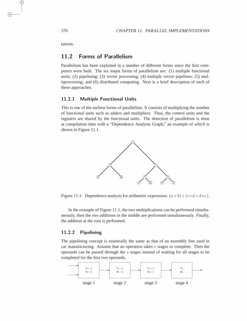
370 CHAPTER 11. PARALLEL IMPLEMENTATIONS
tations.
11.2 Forms of Parallelism
Parallelism has been exploited in a number of different forms since the firstcom-puters were built. The six major forms of parallelism are: (1) multiple functionalunits; (2) pipelining; (3) vector processing; (4) multiple vector pipelines; (5) mul-tiprocessing; and (6) distributed computing. Next is a brief description of each ofthese approaches.
11.2.1 Multiple Functional Units
This is one of the earliest forms of parallelism. It consists of multiplying the numberof functional units such as adders and multipliers. Thus, the control units and theregisters are shared by the functional units. The detection of parallelism isdoneat compilation time with a “Dependence Analysis Graph,” an example of which isshown in Figure 11.1.
+
+ +
a b * *
c d e f
Figure 11.1: Dependence analysis for arithmetic expression:(a+b)+(c∗d+d∗e).
In the example of Figure 11.1, the two multiplications can be performed simulta-neously, then the two additions in the middle are performed simultaneously. Finally,the addition at the root is performed.
11.2.2 Pipelining
The pipelining concept is essentially the same as that of an assembly line used incar manufacturing. Assume that an operation takess stages to complete. Then theoperands can be passed through thes stages instead of waiting for all stages to becompleted for the first two operands.
-
-xi−3yi−3
-
stage 1
xi−2yi−2
-
stage 2
xi−1yi−1
-
stage 3
xi
yi-
stage 4
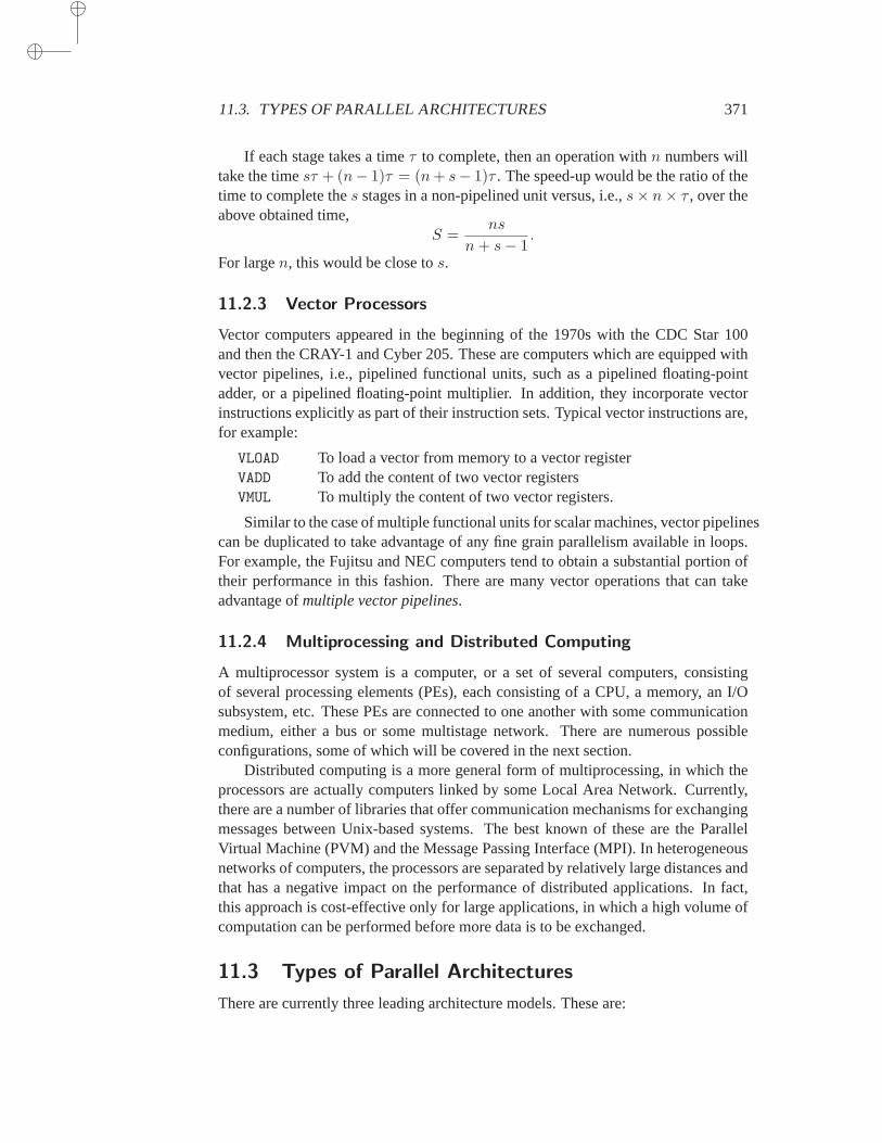
11.3. TYPES OF PARALLEL ARCHITECTURES 371
If each stage takes a timeτ to complete, then an operation withn numbers willtake the timesτ + (n− 1)τ = (n+ s− 1)τ . The speed-up would be the ratio of thetime to complete thes stages in a non-pipelined unit versus, i.e.,s× n× τ , over theabove obtained time,
S =ns
n+ s− 1.
For largen, this would be close tos.
11.2.3 Vector Processors
Vector computers appeared in the beginning of the 1970s with the CDC Star 100and then the CRAY-1 and Cyber 205. These are computers which are equipped withvector pipelines, i.e., pipelined functional units, such as a pipelined floating-pointadder, or a pipelined floating-point multiplier. In addition, they incorporate vectorinstructions explicitly as part of their instruction sets. Typical vector instructions are,for example:
VLOAD To load a vector from memory to a vector registerVADD To add the content of two vector registersVMUL To multiply the content of two vector registers.
Similar to the case of multiple functional units for scalar machines, vector pipelinescan be duplicated to take advantage of any fine grain parallelism available in loops.For example, the Fujitsu and NEC computers tend to obtain a substantial portion oftheir performance in this fashion. There are many vector operations that can takeadvantage ofmultiple vector pipelines.
11.2.4 Multiprocessing and Distributed Computing
A multiprocessor system is a computer, or a set of several computers, consistingof several processing elements (PEs), each consisting of a CPU, a memory, an I/Osubsystem, etc. These PEs are connected to one another with some communicationmedium, either a bus or some multistage network. There are numerous possibleconfigurations, some of which will be covered in the next section.
Distributed computing is a more general form of multiprocessing, in which theprocessors are actually computers linked by some Local Area Network. Currently,there are a number of libraries that offer communication mechanisms for exchangingmessages between Unix-based systems. The best known of these are theParallelVirtual Machine (PVM) and the Message Passing Interface (MPI). In heterogeneousnetworks of computers, the processors are separated by relatively large distances andthat has a negative impact on the performance of distributed applications. In fact,this approach is cost-effective only for large applications, in which a highvolume ofcomputation can be performed before more data is to be exchanged.
11.3 Types of Parallel Architectures
There are currently three leading architecture models. These are:
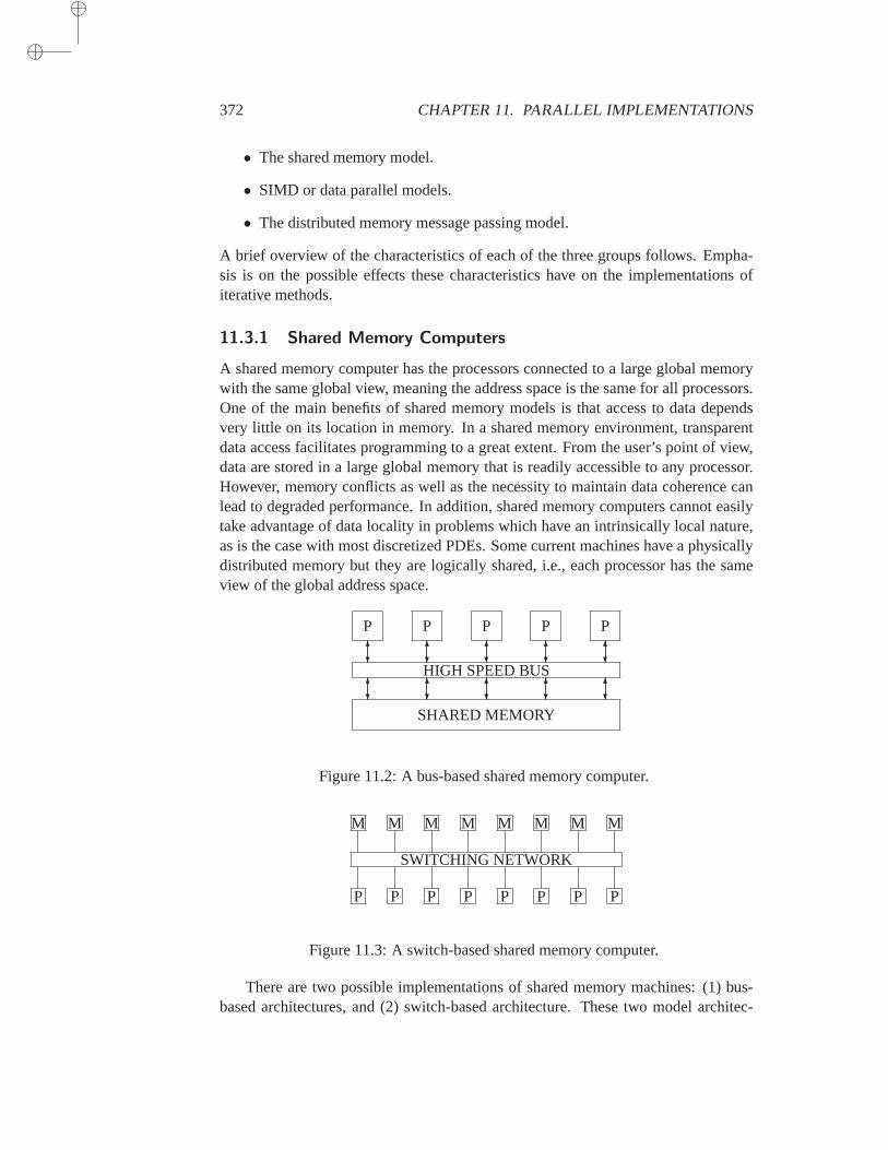
372 CHAPTER 11. PARALLEL IMPLEMENTATIONS
• The shared memory model.
• SIMD or data parallel models.
• The distributed memory message passing model.
A brief overview of the characteristics of each of the three groups follows. Empha-sis is on the possible effects these characteristics have on the implementations ofiterative methods.
11.3.1 Shared Memory Computers
A shared memory computer has the processors connected to a large globalmemorywith the same global view, meaning the address space is the same for all processors.One of the main benefits of shared memory models is that access to data dependsvery little on its location in memory. In a shared memory environment, transparentdata access facilitates programming to a great extent. From the user’s pointof view,data are stored in a large global memory that is readily accessible to any processor.However, memory conflicts as well as the necessity to maintain data coherencecanlead to degraded performance. In addition, shared memory computers cannot easilytake advantage of data locality in problems which have an intrinsically local nature,as is the case with most discretized PDEs. Some current machines have a physicallydistributed memory but they are logically shared, i.e., each processor has the sameview of the global address space.
P P P P P
SHARED MEMORY
HIGH SPEED BUS? ? ? ? ?6 6 6 6 6
6 6 6 6 6? ? ? ? ?
Figure 11.2: A bus-based shared memory computer.
P P P P P P P P
SWITCHING NETWORK
M M M M M M M M
Figure 11.3: A switch-based shared memory computer.
There are two possible implementations of shared memory machines: (1) bus-based architectures, and (2) switch-based architecture. These two model architec-

11.3. TYPES OF PARALLEL ARCHITECTURES 373
tures are illustrated in Figure 11.2 and Figure 11.3, respectively. So far,shared mem-ory computers have been implemented more often with buses than with switchingnetworks.
Buses are the backbone for communication between the different units of mostcomputers. Physically, a bus is nothing but a bundle of wires, made of eitherfiberor copper. These wires carry information consisting of data, control signals, anderror correction bits. The speed of a bus, often measured in Megabytesper secondand called thebandwidthof the bus, is determined by the number of lines in the busand the clock rate. Often, the limiting factor for parallel computers based on busarchitectures is the bus bandwidth rather than the CPU speed.
The primary reason why bus-based multiprocessors are more common than switch-based ones is that the hardware involved in such implementations is simple. On theother hand, the difficulty with bus-based machines is that the number of processorswhich can be connected to the memory will be small in general. Typically, the busistimeshared, meaning slices of time are allocated to the different clients (processors,IO processors, etc.) that request its use.
In a multiprocessor environment, the bus can easily be saturated. Severalreme-dies are possible. The first, and most common, remedy is to attempt to reduce trafficby addinglocal memoriesor cachesattached to each processor. Since a data itemused by a given processor is likely to be reused by the same processor inthe nextinstructions, storing the data item in local memory will help reduce traffic in general.However, this strategy causes some difficulties due to the requirement to maintaindata coherence. If Processor (A) reads some data from the shared memory, and Pro-cessor (B) modifies the same data in shared memory, immediately after, the resultistwo copies of the same data that have different values. A mechanism shouldbe put inplace to ensure that the most recent update of the data is always used. The additionaloverhead incurred by such memory coherence operations may well offset the savingsinvolving memory traffic.
The main features here are the switching network and the fact that a globalmem-ory is shared by all processors through the switch. There can bep processors on oneside connected top memory units or banks on the other side. Alternative designsbased on switches connectp processors to each other instead ofp memory banks.The switching network can be a crossbar switch when the number of processors issmall. A crossbar switch is analogous to a telephone switch board and allowspinputs to be connected tom outputs without conflict. Since crossbar switches forlarge numbers of processors are typically expensive they are replaced by multistagenetworks. Signals travel across a small number of stages consisting of anarray ofelementary switches, e.g.,2× 2 or 4× 4 switches.
There have been two ways of exploiting multistage networks. Incircuit switch-ing networks, the elementary switches are set up by sending electronic signalsacrossall of the switches. The circuit is set up once in much the same way that telephonecircuits are switched in a switchboard. Once the switch has been set up, communi-
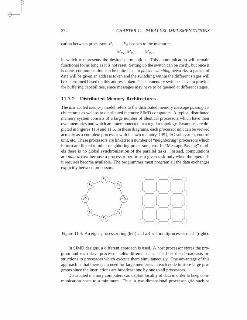
374 CHAPTER 11. PARALLEL IMPLEMENTATIONS
cation between processorsP1, . . . , Pn is open to the memories
Mπ1 ,Mπ2 , . . . ,Mπn ,
in which π represents the desired permutation. This communication will remainfunctional for as long as it is not reset. Setting up the switch can be costly, but once itis done, communication can be quite fast. Inpacket switchingnetworks, a packet ofdata will be given an address token and the switching within the different stages willbe determined based on this address token. The elementary switches have toprovidefor buffering capabilities, since messages may have to be queued at different stages.
11.3.2 Distributed Memory Architectures
Thedistributed memorymodel refers to the distributed memorymessage passingar-chitectures as well as to distributed memory SIMD computers. A typical distributedmemory system consists of a large number of identical processors which have theirown memories and which are interconnected in a regular topology. Examples are de-picted in Figures 11.4 and 11.5. In these diagrams, each processor unit can be viewedactually as a complete processor with its own memory, CPU, I/O subsystem, controlunit, etc. These processors are linked to a number of “neighboring” processors whichin turn are linked to other neighboring processors, etc. In “Message Passing” mod-els there is no global synchronization of the parallel tasks. Instead, computationsaredata drivenbecause a processor performs a given task only when the operandsit requires become available. The programmer must program all the data exchangesexplicitly between processors.
P1
P2
P3
P4
P5
P6
P7
P8
Figure 11.4: An eight-processor ring (left) and a4× 4 multiprocessor mesh (right).
In SIMD designs, a different approach is used. A host processor stores the pro-gram and each slave processor holds different data. The host then broadcasts in-structions to processors which execute them simultaneously. One advantage of thisapproach is that there is no need for large memories in each node to store large pro-grams since the instructions are broadcast one by one to all processors.
Distributed memory computers can exploit locality of data in order to keep com-munication costs to a minimum. Thus, a two-dimensional processor grid such as

11.3. TYPES OF PARALLEL ARCHITECTURES 375
the one depicted in Figure 11.4 is perfectly suitable for solving discretized ellipticPartial Differential Equations (e.g., by assigning each grid point to a correspondingprocessor) because some iterative methods for solving the resulting linearsystemswill require only interchange of data between adjacent grid points. A goodgeneralpurpose multiprocessor must have powerfulmapping capabilitiesbecause it shouldbe capable of easily emulating many of the common topologies such as 2-D and 3-Dgrids or linear arrays, FFT-butterflies, finite element meshes, etc.
Three-dimensional configurations have also been popular.
10 11
010010
101
111110
100
010 011
001000
Figure 11.5: Then-cubes of dimensionsn = 1, 2, 3.
Hypercubes are highly concurrent multiprocessors based on the binary n-cube topol-ogy which is well known for its rich interconnection capabilities. A parallel processorbased on then-cube topology, called ahypercubehereafter, consists of2n identicalprocessors, interconnected withn neighbors. A3-cube can be represented as an ordi-nary cube in three dimensions where the vertices are the8 = 23 nodes of the 3-cube;see Figure 11.5. More generally, one can construct ann-cube as follows: First, the2n nodes are labeled by the2n binary numbers from0 to 2n−1. Then a link betweentwo nodes is drawn if and only if their binary numbers differ by one (and only one)bit.
An n-cube graph can be constructed recursively from lower dimensional cubes.More precisely, consider two identical(n−1)-cubes whose vertices are labeled like-wise from 0 to2n−1. By joining every vertex of the first(n − 1)-cube to the vertexof the second having the same number, one obtains ann-cube. Indeed, it suffices torenumber the nodes of the first cube as0 ∧ ai and those of the second as1 ∧ ai
whereai is a binary number representing the two similar nodes of the(n− 1)-cubesand where∧ denotes the concatenation of binary numbers.
Distributed memory computers come in two different designs, namely, SIMDand MIMD. Many of the early projects have adopted the SIMD organization. Forexample, the historical ILLIAC IV Project of the University of Illinois was amachinebased on a mesh topology where all processors execute the same instructions.
SIMD distributed processors are sometimes called array processors because ofthe regular arrays that they constitute. In this category, systolic arrays can be clas-sified as an example of distributed computing. Systolic arrays, which popularin the
376 CHAPTER 11. PARALLEL IMPLEMENTATIONS
1980s, are organized in connected cells, which are programmed (possibly micro-coded) to perform only one of a few operations. All the cells are synchronized andperform the same task. Systolic arrays are designed in VLSI technology and aremeant to be used for special purpose applications, primarily in signal processing.
In the last few years, parallel computing technologies have seen a healthymatu-ration. Currently, the architecture of choice is the distributed memory machine usingmessage passing. There is no doubt that this is due to the availability of excellentcommunication software, such the Message Passing Interface (MPI), see [156]. Inaddition, the topology
is often hidden from the user, so there is no need to code communication onspecific configurations such as hypercubes. Since this mode of computing has pen-etrated the applications areas, and industrial applications it is likely to remain forsome time.
11.4 Types of Operations
Now consider two prototype Krylov subspace techniques, namely, the precondi-tioned Conjugate Gradient method for the symmetric case and the preconditionedGMRES algorithm for the nonsymmetric case. It should be emphasized that allKrylov subspace techniques require the same basic operations.
Consider Algorithm 9.1. The first step when implementing this algorithm on ahigh-performance computer is identifying the main operations that it requires. Wedistinguish five types of operations, which are: (1) Preconditioner setup; (2) Matrixvector multiplications; (3) Vector updates; (4) Dot products; and (5) Preconditioningoperations. In this list the potential bottlenecks are (1), setting up the preconditionerand (5), solving linear systems withM , i.e., the preconditioning operation. Section11.6 discusses the implementation of traditional preconditioners, and the last twochapters are devoted to preconditioners that are specialized to parallel environments.Next come the matrix-by-vector products which deserve particular attention. Therest of the algorithm consists essentially of dot products and vector updates whichdo not cause significant difficulties in parallel machines, although inner products canlead to some loss of efficiency on certain types of computers with large numbers ofprocessors.
If we now consider the GMRES algorithm, the only new operation here withrespect to the Conjugate Gradient method is the orthogonalization of the vector Avi
against the previousv’s. The usual way to accomplish this is via the modified Gram-Schmidt process, which is basically a sequence of subprocesses of theform:
• Computeα = (y, v).
• Computey := y − αv.
This orthogonalizes a vectory against another vectorv of norm one. Thus, the outerloop of the modified Gram-Schmidt is sequential, but the inner loop, i.e., each sub-process, can be parallelized by dividing the inner product and SAXPY operations
11.4. TYPES OF OPERATIONS 377
among processors. Although this constitutes a perfectly acceptable approach for asmall number of processors, the elementary subtasks may be too small to be efficienton a large number of processors. An alternative for this case is to use a standardGram-Schmidt process with reorthogonalization. This replaces the previous sequen-tial orthogonalization process by a matrix operation of the formy = y−V V T y, i.e.,BLAS-1 kernels are replaced by BLAS-2 kernels.
Recall that the next level of BLAS, i.e., level 3 BLAS, exploits blocking indense matrix operations in order to obtain performance on machines with hierarchi-cal memories. Unfortunately, level 3 BLAS kernels cannot be exploited here becauseat every step, there is only one vector to orthogonalize against all previous ones. Thismay be remedied by using block Krylov methods.
Vector operations, such as linear combinations of vectors and dot-products areusually the simplest to implement on any computer. In shared memory computers,compilers are capable of recognizing these operations and invoking the appropriatemachine instructions, possibly vector instructions. We consider now these operationsin turn.
Vector Updates Operations of the form
y(1:n) = y(1:n) + a * x(1:n),
wherea is a scalar andy andx two vectors, are known asvector updatesor SAXPYoperations. They are typically straightforward to implement in all three machinemodels discussed earlier. For example, the above FORTRAN-90 code segment canbe used on most shared memory (’symmetric multiprocessing’) and the compiler willtranslate it into the proper parallel version.
On distributed memory computers, some assumptions must be made about theway in which the vectors are distributed. The main assumption is that the vectorsxandy are distributed in the same manner among the processors, meaning the indicesof the components of any vector that are mapped to a given processor are the same.In this case, the vector-update operation will be translated intop independent vectorupdates, requiring no communication. Specifically, ifnloc is the number of variableslocal to a given processor, this processor will simply execute a vector loop of the form
y(1:nloc) = y(1:nloc) + a * x(1:nloc)
and all processors will execute a similar operation simultaneously.
Dot products A number of operations use all the components of a given vector tocompute a single floating-point result which is then needed by all processors. Theseare termedReduction Operationsand the dot product is the prototype example. Adistributed version of the dot-product is needed to compute the inner product of twovectorsx and y that are distributed the same way across the processors. In fact,to be more specific, this distributed dot-product operation should compute theinnerproductt = xT y of these two vectors and then make the resultt available in each
378 CHAPTER 11. PARALLEL IMPLEMENTATIONS
processor. Typically, this result is needed to perform vector updates or other opera-tions in each node. For a large number of processors, this sort of operation can bedemanding in terms of communication costs. On the other hand, parallel computerdesigners have become aware of their importance and are starting to provide hard-ware and software support for performingglobal reduction operationsefficiently.Reduction operations that can be useful include global sums, global max/mincal-culations, etc. A commonly adopted convention provides a single subroutine for allthese operations, and passes the type of operation to be performed (add, max, min,multiply,. . . ) as one of the arguments. With this in mind, a distributed dot-productfunction can be programmed roughly as follows (using C syntax).
tloc = DDOT(nrow, x, incx, y, incy);
MPI\_Allreduce(\&t, \&tsum, 1, MPI\_DOUBLE, MPI\_SUM, comm);
The function DDOT performs the usual BLAS-1 dot product ofx andy with stridesincx and incy, respectively. The MPIAllreduce operation, which is called with“MPI SUM” as the operation-type parameter, sums all the variables “tloc” from eachprocessor and put the resulting global sum in the variabletsum in each processor.
11.5 Matrix-by-Vector Products
Matrix-by-vector multiplications (sometimes called “Matvecs” for short) are rela-tively easy to implement efficiently on high performance computers. For a descrip-tion of storage formats for sparse matrices, see Chapter 3. We will first discussmatrix-by-vector algorithms without consideration of sparsity. Then we will coversparse Matvec operations for a few different storage formats.
The computational kernels for performing sparse matrix operations such as matrix-by-vector products are intimately associated with the data structures used. How-ever, there are a few general approaches that are common to different algorithms formatrix-by-vector products which can be described for dense matrices. Two popu-lar ways of performing these operations are the inner product form andthe SAXPYform. In the inner product form for computingy = Ax, the componentyi is obtainedas a dot-product of thei-th row of i and the vectorx. The SAXPY form computesy as a linear combination of the columns ofA, specifically as the sum ofxiA:,i fori = 1, . . . , n. A third option consists of performing the product by diagonals. Thisoption bears no interest in the dense case, but it is at the basis of many importantmatrix-by-vector algorithms in the sparse case as will be seen shortly.
11.5.1 The CSR and CSC Formats
Recall that the CSR data-structure seen in Chapter 3 consists of three arrays: a realarrayA(1:nnz)to store the nonzero elements of the matrix row-wise, an integer arrayJA(1:nnz)to store the column positions of the elements in the real arrayA, and,finally, a pointer arrayIA(1:n+1), thei-th entry of which points to the beginning ofthei-th row in the arraysA andJA. To perform the matrix-by-vector producty = Ax
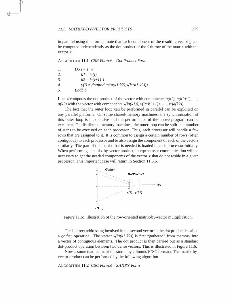
11.5. MATRIX-BY-VECTOR PRODUCTS 379
in parallel using this format, note that each component of the resulting vectory canbe computed independently as the dot product of thei-th row of the matrix with thevectorx.
ALGORITHM 11.1 CSR Format – Dot Product Form
1. Do i = 1, n2. k1 = ia(i)3. k2 = ia(i+1)-14. y(i) = dotproduct(a(k1:k2),x(ja(k1:k2)))5. EndDo
Line 4 computes the dot product of the vector with componentsa(k1), a(k1+1),· · ·,a(k2)with the vector with componentsx(ja(k1)), x(ja(k1+1)),· · ·, x(ja(k2)).
The fact that the outer loop can be performed in parallel can be exploited onany parallel platform. On some shared-memory machines, the synchronization ofthis outer loop is inexpensive and the performance of the above programcan beexcellent. On distributed memory machines, the outer loop can be split in a numberof steps to be executed on each processor. Thus, each processor will handle a fewrows that are assigned to it. It is common to assign a certain number of rows (oftencontiguous) to each processor and to also assign the component of each of the vectorssimilarly. The part of the matrix that is needed is loaded in each processor initially.When performing a matrix-by-vector product, interprocessor communication will benecessary to get the needed components of the vectorx that do not reside in a givenprocessor. This important case will return in Section 11.5.5.
+
+
+
+
DotProductGather
*
x(*) a(i,*)
x(1:n)
y(i)
Figure 11.6: Illustration of the row-oriented matrix-by-vector multiplication.
The indirect addressing involved in the second vector in the dot productis calleda gather operation. The vectorx(ja(k1:k2)) is first “gathered” from memory intoa vector of contiguous elements. The dot product is then carried out as astandarddot-product operation between two dense vectors. This is illustrated in Figure 11.6.
Now assume that the matrix is stored by columns (CSC format). The matrix-by-vector product can be performed by the following algorithm.
ALGORITHM 11.2 CSC Format – SAXPY Form
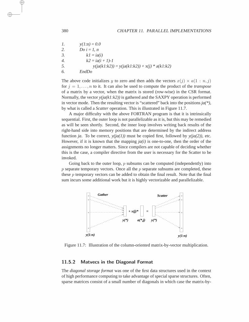
380 CHAPTER 11. PARALLEL IMPLEMENTATIONS
1. y(1:n) = 0.02. Do i = 1, n3. k1 = ia(i)4. k2 = ia(i + 1)-15. y(ja(k1:k2)) = y(ja(k1:k2)) + x(j) * a(k1:k2)6. EndDo
The above code initializesy to zero and then adds the vectorsx(j) × a(1 : n, j)for j = 1, . . . , n to it. It can also be used to compute the product of thetransposeof a matrix by a vector, when the matrix is stored (row-wise) in the CSR format.Normally, the vectory(ja(k1:k2))is gathered and the SAXPY operation is performedin vector mode. Then the resulting vector is “scattered” back into the positionsja(*) ,by what is called aScatteroperation. This is illustrated in Figure 11.7.
A major difficulty with the above FORTRAN program is that it is intrinsicallysequential. First, the outer loop is not parallelizable as it is, but this may be remediedas will be seen shortly. Second, the inner loop involves writing back resultsof theright-hand side into memory positions that are determined by the indirect addressfunction ja. To be correct,y(ja(1)) must be copied first, followed byy(ja(2)), etc.However, if it is known that the mappingja(i) is one-to-one, then the order of theassignments no longer matters. Since compilers are not capable of deciding whetherthis is the case, a compiler directive from the user is necessary for the Scatter to beinvoked.
Going back to the outer loop,p subsums can be computed (independently) intop separate temporary vectors. Once all thep separate subsums are completed, thesethesep temporary vectors can be added to obtain the final result. Note that the finalsum incurs some additional work but it is highly vectorizable and parallelizable.
+
+
+
+
+
+
+
+
Gather
+ x(j)*
y(1:n)
y(*)
y(1:n)
=
Scatter
y(*) a(*,j)
Figure 11.7: Illustration of the column-oriented matrix-by-vector multiplication.
11.5.2 Matvecs in the Diagonal Format
Thediagonal storage formatwas one of the first data structures used in the contextof high performance computing to take advantage of special sparse structures. Often,sparse matrices consist of a small number of diagonals in which case the matrix-by-
11.5. MATRIX-BY-VECTOR PRODUCTS 381
vector product can be performed by diagonals. There are again different variants ofMatvec algorithms for the diagonal format, related to different orderings of the loopsin the basic FORTRAN program. Recall that the matrix is stored in a rectangulararraydiag(1:n,1:ndiag)and the offsets of these diagonals from the main diagonalmay be stored in a small integer arrayoffset(1:ndiag). Consider a “dot-product”variant first.
ALGORITHM 11.3 DIA Format – Dot Product Form
1. Do i = 1, n2. tmp = 0.0d03. Do j = 1, ndiag4. tmp = tmp + diag(i,j)*x(i+offset(j))5. EndDo6. y(i) = tmp7. EndDo
In a second variant, the vectory is initialized to zero, and thenx is multiplied byeach of the diagonals and the separate results are added toy. The innermost loop inthis computation is sometimes called aTriad operation.
ALGORITHM 11.4 Matvec in Triad Form
1. y = 0.0d02. Do j = 1, ndiag3. joff = offset(j)4. i1 = max(1, 1-offset(j))5. i2 = min(n, n-offset(j))6. y(i1:i2) = y(i1:i2) + diag(i1:i2,j)*x(i1+joff:i2+joff)7. EndDo
Good speeds can be reached on vector machines for large enough matrices. Adrawback with diagonal schemes is that it are not general. For generalsparse ma-trices, we can either generalize the diagonal storage scheme or reorderthe matrix inorder to obtain a diagonal structure. The simplest generalization is the Ellpack-ItpackFormat.
11.5.3 The Ellpack-Itpack Format
The Ellpack-Itpack (or Ellpack) format is of interest only for matrices whose maxi-mum number of nonzeros per row,jmax, is small. The nonzero entries are stored ina real arrayae(1:n,1:jmax). Along with this is integer arrayjae(1:n,1:jmax)whichstores the column indices of each corresponding entry inae. Similar to the diagonalscheme, there are also two basic ways of implementing a matrix-by-vector productwhen using the Ellpack format. We begin with an analogue of Algorithm 11.3.
382 CHAPTER 11. PARALLEL IMPLEMENTATIONS
ALGORITHM 11.5 Ellpack Format – Dot-Product Form
1. Do i = 1, n2. yi = 03. Do j = 1, ncol4. yi = yi + ae(i,j) * x(jae(i,j))5. EndDo6. y(i) = yi7. EndDo
If the number of nonzero elements per row varies substantially, many zero ele-ments must be stored unnecessarily. Then the scheme becomes inefficient. As anextreme example, if all rows are very sparse except for one of them which is full,then the arraysae, jae must be fulln × n arrays, containing mostly zeros. This isremedied by a variant of the format which is called thejagged diagonal format.
11.5.4 The Jagged Diagonal Format
The Jagged Diagonal (JAD) format can be viewed as a generalization ofthe Ellpack-Itpack format which removes the assumption on the fixed length rows. To buildthejagged diagonal structure, start from the CSR data structure and sort the rows of thematrix by decreasing number of nonzero elements. To build the first “j-diagonal”extract the first element from each row of the CSR data structure. The second jaggeddiagonal consists of the second elements of each row in the CSR data structure.The third, fourth,. . ., jagged diagonals can then be extracted in the same fashion.The lengths of the successive j-diagonals decreases. The number of j-diagonals thatcan be extracted is equal to the number of nonzero elements of the first rowof thepermuted matrix, i.e., to the largest number of nonzero elements per row. To storethis data structure, three arrays are needed: a real arrayDJ to store the values ofthe jagged diagonals, the associated arrayJDIAG which stores the column positionsof these values, and a pointer arrayIDIAG which points to the beginning of eachj-diagonal in theDJ, JDIAGarrays.
Example 11.1. Consider the following matrix and its sorted versionPA:
A =
1. 0. 2. 0. 0.3. 4. 0. 5. 0.0. 6. 7. 0. 8.0. 0. 9. 10. 0.0. 0. 0. 11. 12.
→ PA =
3. 4. 0. 5. 0.0. 6. 7. 0. 8.1. 0. 2. 0. 0.0. 0. 9. 10. 0.0. 0. 0. 11. 12.
The rows ofPA have been obtained from those ofA by sorting them by numberof nonzero elements, from the largest to the smallest number. Then the JAD datastructure forA is as follows:
11.5. MATRIX-BY-VECTOR PRODUCTS 383
DJ 3. 6. 1. 9. 11. 4. 7. 2. 10. 12. 5. 8.
JDIAG 1 2 1 3 4 2 3 3 4 5 4 5
IDIAG 1 6 11 13
Thus, there are two j-diagonals of full length (five) and one of length two.
A matrix-by-vector product with this storage scheme can be performed by thefollowing code segment.
1. Do j=1, ndiag2. k1 = idiag(j)3. k2 = idiag(j+1) – 14. len = idiag(j+1) – k15. y(1:len) = y(1:len) + dj(k1:k2)*x(jdiag(k1:k2))6. EndDo
Since the rows of the matrixA have been permuted, the above code will computePAx, a permutation of the vectorAx, rather than the desiredAx. It is possibleto permute the result back to the original ordering after the execution of the aboveprogram. This operation can also be performed until the final solution has beencomputed, so that only two permutations on the solution vector are needed, one at thebeginning and one at the end. For preconditioning operations, it may be necessary toperform a permutation before or within each call to the preconditioning subroutines.There are many possible variants of the jagged diagonal format. One variant whichdoes not require permuting the rows is described in Exercise 8.
11.5.5 The Case of Distributed Sparse Matrices
Given a sparse linear system to be solved on a distributed memory environment, it isnatural to map pairs of equations-unknowns to the same processor in a certain prede-termined way. This mapping can be determined automatically by a graph partitioneror it can be assigned ad hoc from knowledge of the problem. Without any loss ofgenerality, the matrix under consideration can be viewed as originating fromthe dis-cretization of a Partial Differential Equation on a certain domain. This is illustratedin Figure 11.8. Assume that each subgraph (or subdomain, in the PDE literature)is assigned to a different processor, although this restriction can be relaxed, i.e., aprocessor can hold several subgraphs to increase parallelism.
A local data structure must be set up in each processor (or subdomain, or sub-graph) which will allow the basic operations such as (global) matrix-by-vector prod-ucts and preconditioning operations to be performed efficiently. The only assumptionto make regarding the mapping is that if row numberi is mapped into processorp,then so is the unknowni, i.e., the matrix is distributed row-wise across the processorsaccording to the distribution of the variables. The graph is assumed to be undirected,i.e., the matrix has a symmetric pattern.
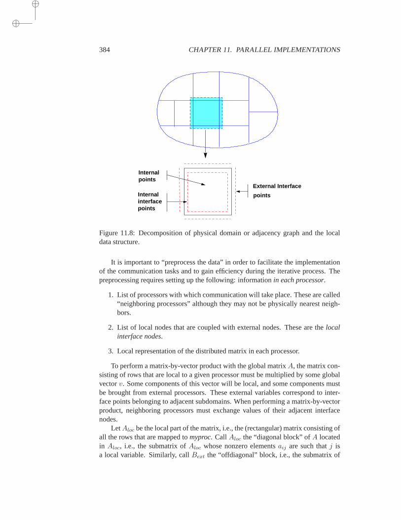
384 CHAPTER 11. PARALLEL IMPLEMENTATIONS
Internalpoints
Internalinterfacepoints
External Interface
points
Figure 11.8: Decomposition of physical domain or adjacency graph and thelocaldata structure.
It is important to “preprocess the data” in order to facilitate the implementationof the communication tasks and to gain efficiency during the iterative process. Thepreprocessing requires setting up the following: informationin each processor.
1. List of processors with which communication will take place. These are called“neighboring processors” although they may not be physically nearestneigh-bors.
2. List of local nodes that are coupled with external nodes. These arethe localinterface nodes.
3. Local representation of the distributed matrix in each processor.
To perform a matrix-by-vector product with the global matrixA, the matrix con-sisting of rows that are local to a given processor must be multiplied by some globalvectorv. Some components of this vector will be local, and some components mustbe brought from external processors. These external variables correspond to inter-face points belonging to adjacent subdomains. When performing a matrix-by-vectorproduct, neighboring processors must exchange values of their adjacent interfacenodes.
LetAloc be the local part of the matrix, i.e., the (rectangular) matrix consisting ofall the rows that are mapped tomyproc. CallAloc the “diagonal block” ofA locatedin Aloc, i.e., the submatrix ofAloc whose nonzero elementsaij are such thatj isa local variable. Similarly, callBext the “offdiagonal” block, i.e., the submatrix of
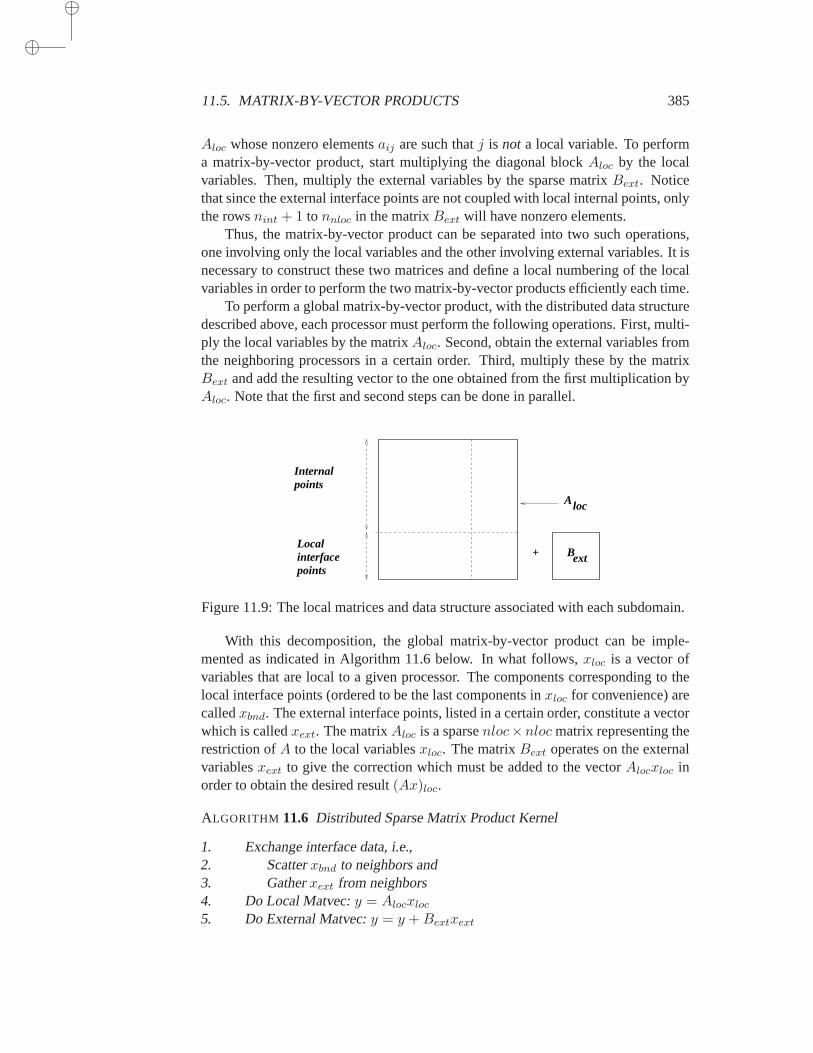
11.5. MATRIX-BY-VECTOR PRODUCTS 385
Aloc whose nonzero elementsaij are such thatj is not a local variable. To performa matrix-by-vector product, start multiplying the diagonal blockAloc by the localvariables. Then, multiply the external variables by the sparse matrixBext. Noticethat since the external interface points are not coupled with local internalpoints, onlythe rowsnint + 1 to nnloc in the matrixBext will have nonzero elements.
Thus, the matrix-by-vector product can be separated into two such operations,one involving only the local variables and the other involving external variables. It isnecessary to construct these two matrices and define a local numbering ofthe localvariables in order to perform the two matrix-by-vector products efficientlyeach time.
To perform a global matrix-by-vector product, with the distributed data structuredescribed above, each processor must perform the following operations. First, multi-ply the local variables by the matrixAloc. Second, obtain the external variables fromthe neighboring processors in a certain order. Third, multiply these by the matrixBext and add the resulting vector to the one obtained from the first multiplication byAloc. Note that the first and second steps can be done in parallel.
Bext
Internalpoints
Localinterfacepoints
+
Aloc
Figure 11.9: The local matrices and data structure associated with each subdomain.
With this decomposition, the global matrix-by-vector product can be imple-mented as indicated in Algorithm 11.6 below. In what follows,xloc is a vector ofvariables that are local to a given processor. The components corresponding to thelocal interface points (ordered to be the last components inxloc for convenience) arecalledxbnd. The external interface points, listed in a certain order, constitute a vectorwhich is calledxext. The matrixAloc is a sparsenloc×nloc matrix representing therestriction ofA to the local variablesxloc. The matrixBext operates on the externalvariablesxext to give the correction which must be added to the vectorAlocxloc inorder to obtain the desired result(Ax)loc.
ALGORITHM 11.6 Distributed Sparse Matrix Product Kernel
1. Exchange interface data, i.e.,2. Scatterxbnd to neighbors and3. Gatherxext from neighbors4. Do Local Matvec:y = Alocxloc
5. Do External Matvec:y = y +Bextxext
386 CHAPTER 11. PARALLEL IMPLEMENTATIONS
An important observation is that the matrix-by-vector products in lines 4 and 5canuse any convenient data structure that will improve efficiency by exploitingknowl-edge on the local architecture. An example of the implementation of this operationis illustrated next:
call bdxchg(nloc,x,y,nproc,proc,ix,ipr,type,xlen,iout)y(1:nloc) = 0.0call amux1 (nloc,x,y,aloc,jaloc,ialoc)nrow = nloc – nbnd + 1call amux1(nrow,x,y(nbnd),aloc,jaloc,ialoc(nloc+1))
The only routine requiring communication isbdxchgwhose purpose is to ex-change interface values between nearest neighbor processors. The first call toamux1performs the operationy := y + Alocxloc, wherey has been initialized to zero priorto the call. The second call toamux1performsy := y + Bextxext. Notice that thedata for the matrixBext is simply appended to that ofAloc, a standard techniqueused for storing a succession of sparse matrices. TheBext matrix acts only on thesubvector ofx which starts at locationnbnd of x. The size of theBext matrix isnrow = nloc− nbnd+ 1.
11.6 Standard Preconditioning Operations
Each preconditioned step requires the solution of a linear system of equations o theform Mz = y. This section only considers those traditional preconditioners, suchas ILU or SOR or SSOR, in which the solution withM is the result of solving tri-angular systems. Since these are commonly used, it is important to explore ways toimplement them efficiently in a parallel environment. It is also important to stressthat the techniques to be described in this section are mostly useful on shared mem-ory computers. Distributed memory computers utilize different strategies. We onlyconsider lower triangular systems of the form
Lx = b. (11.1)
Without loss of generality, it is assumed thatL is unit lower triangular.
11.6.1 Parallelism in Forward Sweeps
Typically in solving a lower triangular system, the solution is overwritten onto theright-hand side on return. In other words, there is one arrayx for both the solutionand the right-hand side. Therefore, the forward sweep for solving a lower triangularsystem with coefficientsal(i, j) and right-hand-sidex is as follows.
ALGORITHM 11.7 Sparse Forward Elimination
1. Do i=2, n2. For (all j such that al(i,j) is nonzero) Do:
11.6. STANDARD PRECONDITIONING OPERATIONS 387
3. x(i) := x(i) – al(i,j) * x(j)4. EndDo5. EndDo
Assume that the matrix is stored row wise in the general Compressed Sparse Row(CSR) format, except that the diagonal elements (ones) are not stored.Then theabove algorithm translates into the following code segment:
1. Do i=2, n2. Do j=ial(i), ial(i+1) – 13. x(i)=x(i) – al(j) * x(jal(j))4. EndDo5. EndDo
The outer loop corresponding to the variablei is sequential. Thej loop is a sparsedot product of theith row ofL and the (dense) vectorx. This dot product may be splitamong the processors and the partial results may be added at the end. However, thelength of the vector involved in the dot product is typically short. So, this approachis quite inefficient in general. We examine next a few alternative approaches. Theregularly structured and the irregularly structured cases are treated separately.
11.6.2 Level Scheduling: the Case of 5-Point Matrices
First, consider an example which consists of a 5-point matrix associated with a4× 3mesh as represented in Figure 11.10. The lower triangular matrix associatedwiththis mesh is represented in the left side of Figure 11.10. The stencil represented inthe right side of Figure 11.10 establishes the data dependence between theunknownsin the lower triangular system solution when considered from the point of view of agrid of unknowns. It tells us that in order to compute the unknown in position(i, j),only the two unknowns in positions(i−1, j) and(i, j−1) are needed . The unknownx11 does not depend on any other variable and can be computed first. Then the valueof x11 can be used to getx1,2 andx2,1 simultaneously. Then these two values willin turn enablex3,1, x2,2 andx1,3 to be obtained simultaneously, and so on. Thus, thecomputation can proceed in wavefronts.
The steps for this wavefront algorithm are shown with dashed lines in Figure11.10. Observe that the maximum degree of parallelism (or vector length, in the caseof vector processing) that can be reached is the minimum ofnx, ny, the number ofmesh points in thex andy directions, respectively, for 2-D problems.
For 3-D problems, the parallelism is of the order of the maximum size of the setsof domain pointsxi,j,k, wherei+ j+k = lev, a constant levellev. It is important tonote that there is little parallelism or vectorization at the beginning and at the endofthe sweep. The degree of parallelism is equal to one initially, and then increases byone for each wave reaching its maximum, and then decreasing back down to one atthe end of the sweep. For example, for a4× 3 grid, the levels (sets of equations thatcan be solved in parallel) are1, 2, 5, 3, 6, 9, 4, 7, 10, 8, 11, and finally12. The first and last few steps may take a heavy toll on achievable speed-ups.
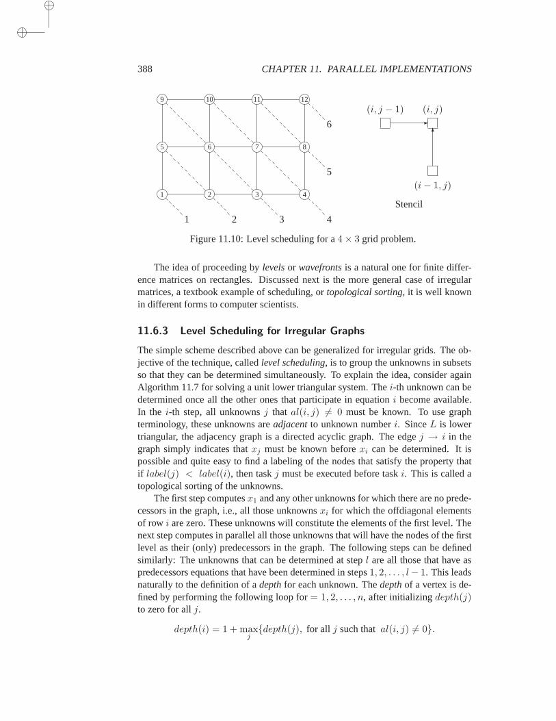
388 CHAPTER 11. PARALLEL IMPLEMENTATIONS
1 2 3 4
5 6 7 8
9 10 11 12
1 2 3 4
5
6
(i, j)
(i− 1, j)
(i, j − 1)-
6
Stencil
Figure 11.10: Level scheduling for a4× 3 grid problem.
The idea of proceeding bylevelsor wavefrontsis a natural one for finite differ-ence matrices on rectangles. Discussed next is the more general case ofirregularmatrices, a textbook example of scheduling, ortopological sorting, it is well knownin different forms to computer scientists.
11.6.3 Level Scheduling for Irregular Graphs
The simple scheme described above can be generalized for irregular grids. The ob-jective of the technique, calledlevel scheduling, is to group the unknowns in subsetsso that they can be determined simultaneously. To explain the idea, consider againAlgorithm 11.7 for solving a unit lower triangular system. Thei-th unknown can bedetermined once all the other ones that participate in equationi become available.In the i-th step, all unknownsj that al(i, j) 6= 0 must be known. To use graphterminology, these unknowns areadjacentto unknown numberi. SinceL is lowertriangular, the adjacency graph is a directed acyclic graph. The edgej → i in thegraph simply indicates thatxj must be known beforexi can be determined. It ispossible and quite easy to find a labeling of the nodes that satisfy the property thatif label(j) < label(i), then taskj must be executed before taski. This is called atopological sorting of the unknowns.
The first step computesx1 and any other unknowns for which there are no prede-cessors in the graph, i.e., all those unknownsxi for which the offdiagonal elementsof row i are zero. These unknowns will constitute the elements of the first level. Thenext step computes in parallel all those unknowns that will have the nodes of the firstlevel as their (only) predecessors in the graph. The following steps canbe definedsimilarly: The unknowns that can be determined at stepl are all those that have aspredecessors equations that have been determined in steps1, 2, . . . , l− 1. This leadsnaturally to the definition of adepthfor each unknown. Thedepthof a vertex is de-fined by performing the following loop for= 1, 2, . . . , n, after initializingdepth(j)to zero for allj.
depth(i) = 1 + maxjdepth(j), for all j such thatal(i, j) 6= 0.
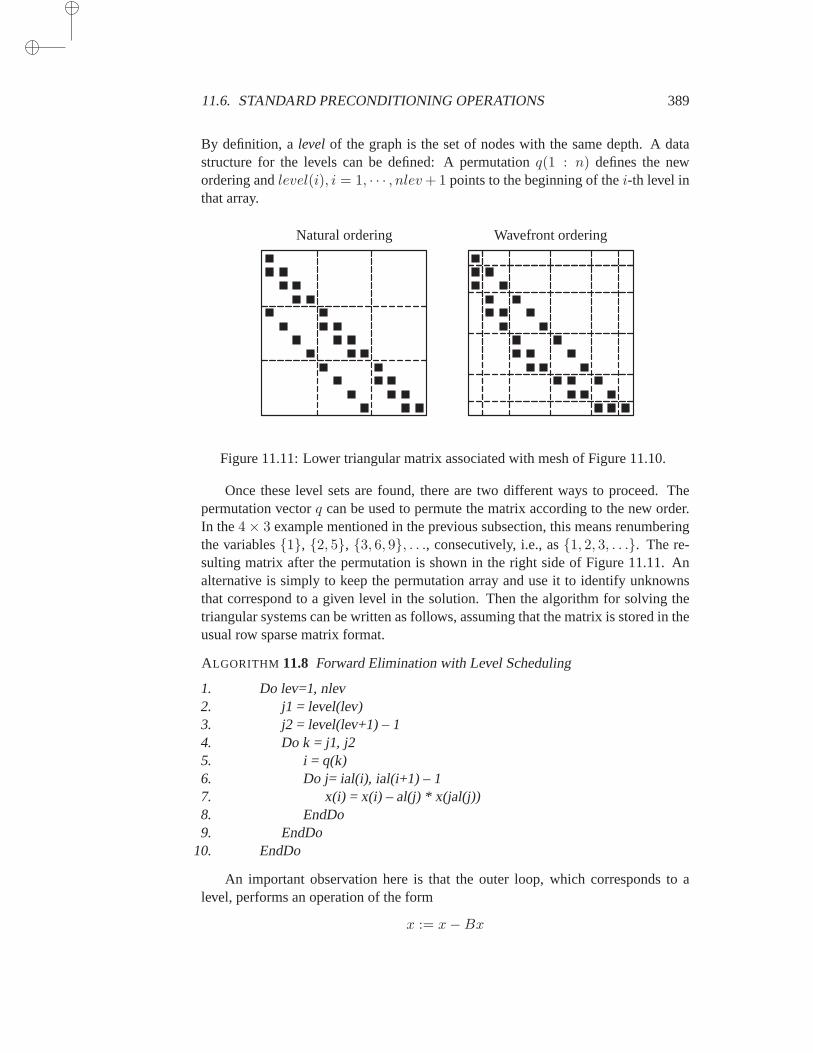
11.6. STANDARD PRECONDITIONING OPERATIONS 389
By definition, alevel of the graph is the set of nodes with the same depth. A datastructure for the levels can be defined: A permutationq(1 : n) defines the newordering andlevel(i), i = 1, · · · , nlev+ 1 points to the beginning of thei-th level inthat array.
Natural ordering Wavefront ordering
Figure 11.11: Lower triangular matrix associated with mesh of Figure 11.10.
Once these level sets are found, there are two different ways to proceed. Thepermutation vectorq can be used to permute the matrix according to the new order.In the4× 3 example mentioned in the previous subsection, this means renumberingthe variables1, 2, 5, 3, 6, 9, . . ., consecutively, i.e., as1, 2, 3, . . .. The re-sulting matrix after the permutation is shown in the right side of Figure 11.11. Analternative is simply to keep the permutation array and use it to identify unknownsthat correspond to a given level in the solution. Then the algorithm for solving thetriangular systems can be written as follows, assuming that the matrix is stored in theusual row sparse matrix format.
ALGORITHM 11.8 Forward Elimination with Level Scheduling
1. Do lev=1, nlev2. j1 = level(lev)3. j2 = level(lev+1) – 14. Do k = j1, j25. i = q(k)6. Do j= ial(i), ial(i+1) – 17. x(i) = x(i) – al(j) * x(jal(j))8. EndDo9. EndDo
10. EndDo
An important observation here is that the outer loop, which corresponds toalevel, performs an operation of the form
x := x−Bx
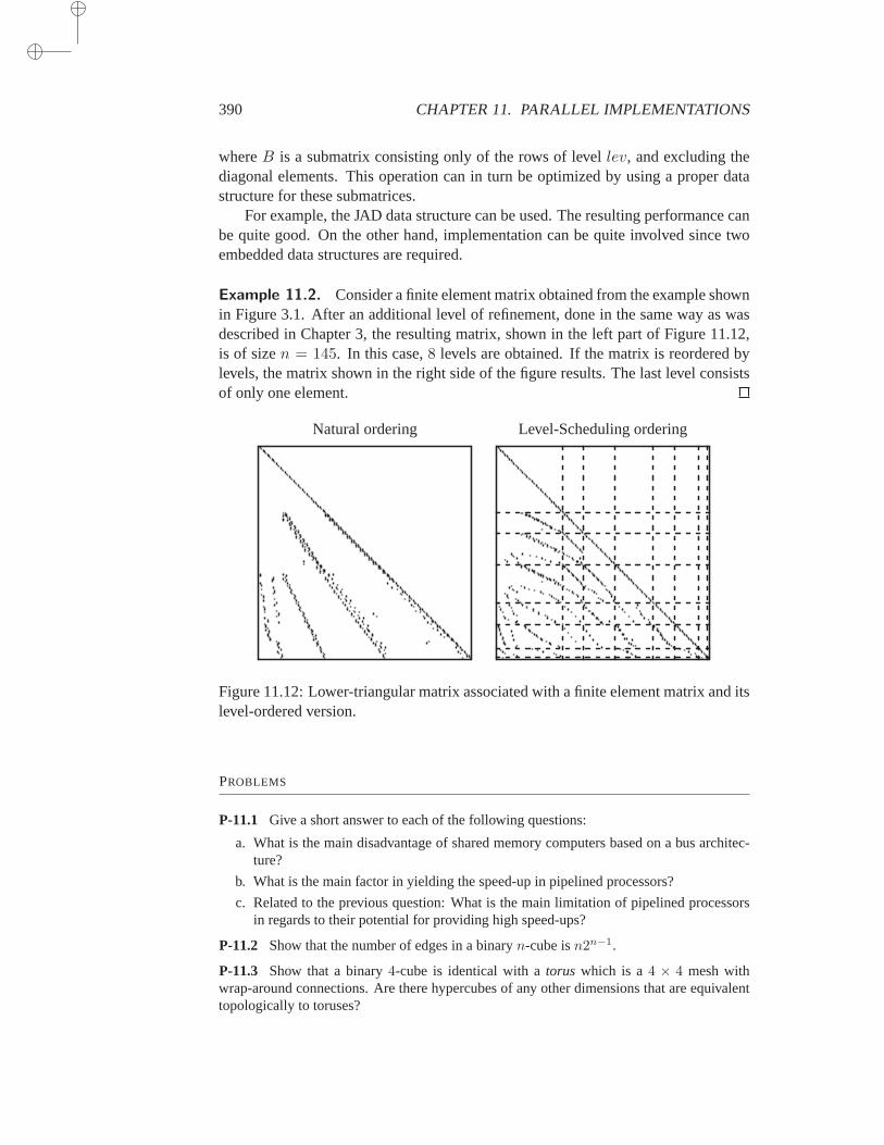
390 CHAPTER 11. PARALLEL IMPLEMENTATIONS
whereB is a submatrix consisting only of the rows of levellev, and excluding thediagonal elements. This operation can in turn be optimized by using a proper datastructure for these submatrices.
For example, the JAD data structure can be used. The resulting performance canbe quite good. On the other hand, implementation can be quite involved since twoembedded data structures are required.
Example 11.2. Consider a finite element matrix obtained from the example shownin Figure 3.1. After an additional level of refinement, done in the same way aswasdescribed in Chapter 3, the resulting matrix, shown in the left part of Figure11.12,is of sizen = 145. In this case,8 levels are obtained. If the matrix is reordered bylevels, the matrix shown in the right side of the figure results. The last level consistsof only one element.
Natural ordering Level-Scheduling ordering
Figure 11.12: Lower-triangular matrix associated with a finite element matrix anditslevel-ordered version.
PROBLEMS
P-11.1 Give a short answer to each of the following questions:
a. What is the main disadvantage of shared memory computers based on a bus architec-ture?
b. What is the main factor in yielding the speed-up in pipelined processors?
c. Related to the previous question: What is the main limitation of pipelined processorsin regards to their potential for providing high speed-ups?
P-11.2 Show that the number of edges in a binaryn-cube isn2n−1.
P-11.3 Show that a binary4-cube is identical with atorus which is a4 × 4 mesh withwrap-around connections. Are there hypercubes of any otherdimensions that are equivalenttopologically to toruses?
11.6. STANDARD PRECONDITIONING OPERATIONS 391
P-11.4 A Gray code of lengthk = 2n is a sequencea0, . . . , ak−1 of n-bit binary numberssuch that (a) any two successive numbers in the sequence differ by one and only one bit; (b)all n-bit binary numbers are represented in the sequence; and (c)a0 andak−1 differ by onebit.
a. Find a Gray code sequence of lengthk = 8 and show the (closed) path defined bythe sequence of nodes of a 3-cube, whose labels are the elements of the Gray codesequence. What type of paths does a Gray code define in a hypercube?
b. To build a “binary reflected” Gray code, start with the trivial Gray code sequence con-sisting of the two one-bit numbers 0 and 1. To build a two-bit Gray code, take the samesequence and insert a zero in front of each number, then take the sequence inreverseorder and insert a one in front of each number. This givesG2 = 00, 01, 11, 10.The process is repeated until ann-bit sequence is generated. Show the binary reflectedGray code sequences of length 2, 4, 8, and 16. Prove (by induction) that this processdoes indeed produce a valid Gray code sequence.
c. Let ann-bit Gray code be given and consider the sub-sequence of all elements whosefirst bit is constant (e.g., zero). Is this ann − 1 bit Gray code sequence? Generalizethis to any of then-bit positions. Generalize further to any set ofk < n bit positions.
d. Use the previous question to find a strategy to map a2n1 × 2n2 mesh into an(n1+n2)-cube.
P-11.5 Consider a ring ofk processors which are characterized by the following communi-cation performance characteristics. Each processor can communicate with its two neighborssimultaneously, i.e., it can send or receive a message while sending or receiving another mes-sage. The time for a message of lengthm to be transmitted between two nearest neighbors isof the form
β +mτ.
a. A message of lengthm is “broadcast” to all processors by sending it fromP1 toP2 andthen fromP2 to P3, etc., until it reaches all destinations, i.e., until it reachesPk. Howmuch time does it take for the message to complete this process?
b. Now split the message into packets of equal size and pipeline the data transfer. Typi-cally, each processor will receive packet numberi from the previous processor, whilesending packeti − 1 it has already received to the next processor. The packets willtravel in chain fromP1 to P2, . . ., to Pk. In other words, each processor executes aprogram that is described roughly as follows:
Do i=1, Num\_packets
Receive Packet number i from Previous Processor
Send Packet number i to Next Processor
EndDo
There are a few additional conditionals. Assume that the number of packets is equal tok− 1. How much time does it take for all packets to reach allk processors? How doesthis compare with the simple method in (a)?
P-11.6 (a) Write a short FORTRAN routine (or C function) which sets upthe level numberof each unknown of an upper triangular matrix. The input matrix is in CSR format and theoutput should be an array of lengthn containing the level number of each node. (b) Whatdata structure should be used to represent levels? Without writing the code, show how todetermine this data structure from the output of your routine. (c) Assuming the data structure

392 CHAPTER 11. PARALLEL IMPLEMENTATIONS
of the levels has been determined, write a short FORTRAN routine (or C function) to solvean upper triangular system using the data structure resulting in the previous question. Showclearly which loop should be executed in parallel.
P-11.7 In the jagged diagonal format described in Section 11.5.4, it is necessary to pre-process the matrix by sorting its rows by decreasing number of rows. What type of sortingshould be used for this purpose?
P-11.8 In the jagged diagonal format described in Section 11.5.4, the matrix had to bepreprocessed by sorting it by rows of decreasing number of elements.
a. What is the main reason it is necessary to reorder the rows?
b. Assume that the same process of extracting one element perrow is used. At some pointthe extraction process will come to a stop and the remainder of the matrix can be putinto a CSR data structure. Write down a good data structure to store the two pieces ofdata and a corresponding algorithm for matrix-by-vector products.
c. This scheme is efficient in many situations but can lead to problems if the first row isvery short. Suggest how to remedy the situation by padding with zero elements, as isdone for the Ellpack format.
P-11.9 Many matrices that arise in PDE applications have a structure that consists of a fewdiagonals and a small number of nonzero elements scattered irregularly in the matrix. Insuch cases, it is advantageous to extract the diagonal part and put the rest in a general sparse(e.g., CSR) format. Write a pseudo-code to extract the main diagonals and the sparse part.As input parameter, the number of diagonals desired must be specified.
NOTES AND REFERENCES. General recommended reading on parallel computing are the booksby Kumar et al. [194]. Foster [131], and Wilkinson and Allen [316]. Trends in high-performancearchitectures seem to come and go rapidly. In the 80s, it seemed that the paradigm of shared memorycomputers with massive parallelism and coarse grain parallelism was sureto win in the long run. Then,a decade ago massive parallelism of the SIMD type dominated the scene for while, with hypercubetopologies at the forefront. Thereafter, computer vendors started mixing message-passing paradigmswith “global address space”. Currently, it appears that distributed heteregenous computing will bedominating the high-performance computing scene for some time to come.Another recent developmentis the advent of network computing or grid-computing.
Until the advent of supercomputing in the mid 1970s, storage schemes for sparse matrices werechosen mostly for convenience as performance was not an issue, in general. The first paper showing theadvantage of diagonal storage schemes in sparse matrix computations isprobably [184]. The discoveryby supercomputer manufacturers of the specificity of sparse matrix computations was the painful real-ization that without hardware support, vector computers could be inefficient. Indeed, the early vectormachines (CRAY) did not have hardware instructions for gather and scatter operations but this wassoon remedied in the second-generation machines. For a detailed account of the beneficial impact ofhardware for “scatter” and “gather” on vector machines, see [201].
Level scheduling is a textbook example of topological sorting in graph theory and was discussedfrom this viewpoint in, e.g., [8, 258, 318]. For the special case of finite difference matrices on rectan-gular domains, the idea was suggested by several authors independently, [288, 289, 155, 252, 10]. Infact, the level scheduling approach described in this chapter is a “greedy” approach and is unlikely tobe optimal. It may be preferable to use abackward scheduling[7] which define the levels from bottomup in the graph. Thus, the last level consists of the leaves of the graph, the previous level consists oftheir predecessors, etc. Instead of static scheduling, it is also possible toperform a dynamic schedulingwhereby the order of the computation is determined at run-time. The advantage over pre-scheduledtriangular solutions is that it allows processors to always execute a task assoon as its predecessors havebeen completed, which reduces idle time. Some of the earlier referenceson implementations and testswih level-scheduling are [30, 257, 165, 30, 37, 7, 8, 294, 296].
Chapter 12
PARALLEL PRECONDITIONERS
This chapter covers a few alternative methods for preconditioning a linear system. These
methods are suitable when the desired goal is to maximize parallelism. The simplest approach is
the diagonal (or Jacobi) preconditioning. Often, this preconditioner is not very useful, since the
number of iterations of the resulting iteration tends to be much larger than the more standard
variants, such as ILU or SSOR. When developing parallel preconditioners, one should beware that
the benefits of increased parallelism are not outweighed by the increased amount of computations.
The main question to ask is whether or not it is possible to find preconditioning techniques that
have a high degree of parallelism, as well as good intrinsic qualities.
12.1 Introduction
As seen in the previous chapter, a limited amount of parallelism can be extractedfrom the standard preconditioners such as ILU and SSOR. Fortunately,a numberof alternative techniques can be developed that are specifically targetedat parallelenvironments. These are preconditioning techniques that would normally not be usedon a standard machine, but only for parallel computers. There are at least three suchtypes of techniques discussed in this chapter. The simplest approach is to use a Jacobior, even better, a block Jacobi approach. In the simplest case, a Jacobi preconditionermay consist of the diagonal or a block-diagonal ofA. To enhance performance, thesepreconditioners can themselves be accelerated by polynomial iterations, i.e.,a secondlevel of preconditioning calledpolynomial preconditioning.
A different strategy altogether is to enhance parallelism by using graph theoryalgorithms, such as graph-coloring techniques. These consist of coloring nodes suchthat two adjacent nodes have different colors. The gist of this approach is that allunknowns associated with the same color can be determined simultaneously in theforward and backward sweeps of the ILU preconditioning operation.
Finally, a third strategy uses generalizations of “partitioning” techniques, whichcan be put in the general framework of “domain decomposition” approaches. Thesewill be covered in detail in the next chapter.
Algorithms are emphasized rather than implementations. There are essentiallytwo types of algorithms, namely, those which can be termedcoarse-grainand thosewhich can be termedfine-grain. In coarse-grain algorithms, the parallel tasks arerelatively big and may, for example, involve the solution of small linear systems.
393
394 CHAPTER 12. PARALLEL PRECONDITIONERS
In fine-grain parallelism, the subtasks can be elementary floating-point operationsor consist of a few such operations. As always, the dividing line between the twoclasses of algorithms is somewhat blurred.
12.2 Block-Jacobi Preconditioners
Overlapping block-Jacobi preconditioning consists of a general block-Jacobi ap-proach as described in Chapter 4, in which the setsSi overlap. Thus, we definethe index sets
Si = j | li ≤ j ≤ riwith
l1 = 1
rp = n
ri > li+1, 1 ≤ i ≤ p− 1
wherep is the number of blocks. Now use the block-Jacobi method with this partic-ular partitioning, or employ the general framework of additive projection processesof Chapter 5, and use an additive projection method onto the sequence of subspaces
Ki = spanVi, Vi = [eli , eli+1, . . . , eri].
Each of the blocks will give rise to a correction of the form
ξ(k+1)i = ξ
(k)i +A−1
i V Ti (b−Ax(k)). (12.1)
One problem with the above formula is related to the overlapping portions of thexvariables. The overlapping sections will receive two different corrections in general.According to the definition of “additive projection processes” seen in Chapter 5, thenext iterate can be defined as
xk+1 = xk +
p∑
i=1
ViA−1i V T
i rk
whererk = b − Axk is the residual vector at the previous iteration. Thus, thecorrections for the overlapping regions simply are added together. It is also possibleto weigh these contributions before adding them up. This is equivalent to redefining(12.1) into
ξ(k+1)i = ξ
(k)i +DiA
−1i V T
i (b−Axk)
in which Di is a nonnegative diagonal matrix of weights. It is typical to weigh anonoverlapping contribution by one and an overlapping contribution by1/k wherekis the number of times the unknown is represented in the partitioning.
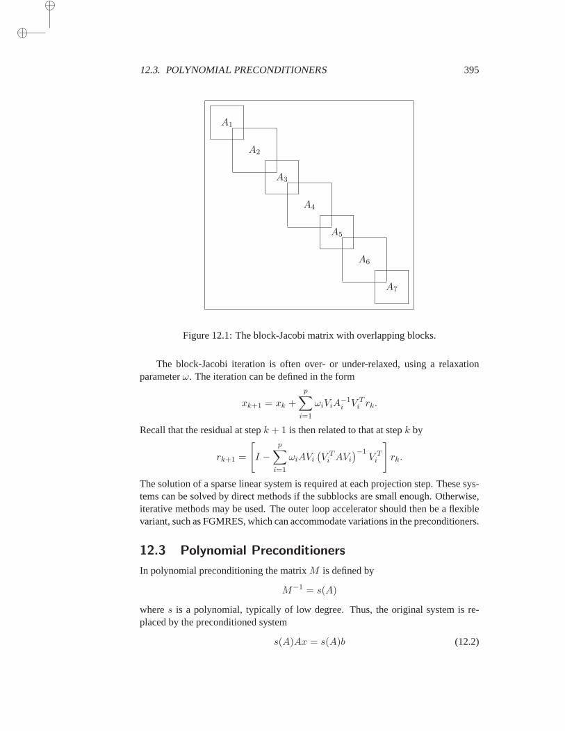
12.3. POLYNOMIAL PRECONDITIONERS 395
A1
A3
A5
A7
A2
A4
A6
Figure 12.1: The block-Jacobi matrix with overlapping blocks.
The block-Jacobi iteration is often over- or under-relaxed, using a relaxationparameterω. The iteration can be defined in the form
xk+1 = xk +
p∑
i=1
ωiViA−1i V T
i rk.
Recall that the residual at stepk + 1 is then related to that at stepk by
rk+1 =
[
I −p∑
i=1
ωiAVi
(V T
i AVi
)−1V T
i
]
rk.
The solution of a sparse linear system is required at each projection step.These sys-tems can be solved by direct methods if the subblocks are small enough. Otherwise,iterative methods may be used. The outer loop accelerator should then be a flexiblevariant, such as FGMRES, which can accommodate variations in the preconditioners.
12.3 Polynomial Preconditioners
In polynomial preconditioning the matrixM is defined by
M−1 = s(A)
wheres is a polynomial, typically of low degree. Thus, the original system is re-placed by the preconditioned system
s(A)Ax = s(A)b (12.2)
396 CHAPTER 12. PARALLEL PRECONDITIONERS
which is then solved by a conjugate gradient-type technique. Note thats(A) andA commute and, as a result, the preconditioned matrix is the same for right or leftpreconditioning. In addition, the matrixs(A) orAs(A) does not need to be formedexplicitly sinceAs(A)v can be computed for any vectorv from a sequence of matrix-by-vector products.
Initially, this approach was motivated by the good performance of matrix-vectoroperations on vector computers for long vectors, e.g., the Cyber 205. However, theidea itself is an old one and has been suggested by Stiefel [276] for eigenvalue cal-culations in the mid 1950s. Next, some of the popular choices for the polynomialsare described.
12.3.1 Neumann Polynomials
The simplest polynomials which has been used is the polynomial of the Neumannseries expansion
I +N +N2 + · · ·+N s
in whichN = I − ωA
andω is a scaling parameter. The above series comes from expanding the inverse ofωA using the splitting
ωA = I − (I − ωA).
This approach can also be generalized by using a splitting of the form
ωA = D − (D − ωA)
whereD can be the diagonal ofA or, more appropriately, a block diagonal ofA.Then,
(ωA)−1 =[D(I − (I − ωD−1A))
]−1
=[I − (I − ωD−1A)
]−1D−1.
Thus, settingN = I − ωD−1A
results in the approximates-term expansion
(ωA)−1 ≈M−1 ≡ [I +N + · · ·+N s]D−1. (12.3)
SinceD−1A = ω−1 [I −N ] , note that
M−1A = [I +N + · · ·+N s]D−1A
=1
ω[I +N + · · ·+N s] (I −N)
=1
ω(I −N s+1).
The matrix operation with the preconditioned matrix can be difficult numerically forlarge s. If the original matrix is Symmetric Positive Definite, thenM−1A is notsymmetric, but it is self-adjoint with respect to theD-inner product; see Exercise 1.
12.3. POLYNOMIAL PRECONDITIONERS 397
12.3.2 Chebyshev Polynomials
The polynomials can be selected to be optimal in some sense, and this leads to theuse of Chebyshev polynomials. The criterion that is used makes the preconditionedmatrix s(A)A as close as possible to the identity matrix in some sense. For exam-ple, the spectrum of the preconditioned matrix can be made as close as possible tothat of the identity. Denoting byσ(A) the spectrum ofA, and byPk the space ofpolynomials of degree not exceedingk, the following may be solved.
Find s ∈ Pk which minimizes:
maxλ∈σ(A)
|1− λs(λ)|. (12.4)
Unfortunately, this problem involves all the eigenvalues ofA and is harder to solvethan the original problem. Usually, problem (12.4) is replaced by the problem
Find s ∈ Pk which minimizes:
maxλ∈E|1− λs(λ)|, (12.5)
which is obtained from replacing the setσ(A) by some continuous setE that enclosesit. Thus, a rough idea of the spectrum of the matrixA is needed. Consider first theparticular case whereA is Symmetric Positive Definite, in which caseE can be takento be an interval[α, β] containing the eigenvalues ofA.
A variation of Theorem 6.25 is that for any real scalarγ such withγ ≤ α, theminimum
minp∈Pk,p(γ)=1
maxt∈[α,β]
|p(t)|
is reached for the shifted and scaled Chebyshev polynomial of the first kind,
Ck(t) ≡Ck
(
1 + 2 α−tβ−α
)
Ck
(
1 + 2α−γβ−α
) .
Of interest is the case whereγ = 0 which gives the polynomial
Tk(t) ≡1
σkCk
(β + α− 2t
β − α
)
with σk ≡ Ck
(β + α
β − α
)
.
Denote the center and mid-width of the interval[α, β], respectively, by
θ ≡ β + α
2, δ ≡ β − α
2.
Using these parameters instead ofα, β, the above expressions then become
Tk(t) ≡1
σkCk
(θ − tδ
)
with σk ≡ Ck
(θ
δ
)
.

398 CHAPTER 12. PARALLEL PRECONDITIONERS
The three-term recurrence for the Chebyshev polynomials results in the followingthree-term recurrences:
σk+1 = 2θ
δσk − σk−1, k = 1, 2 . . . ,
withσ1 =
θ
δ, σ0 = 1,
and
Tk+1(t) ≡1
σk+1
[
2θ − tδ
σkTk(t)− σk−1Tk−1(t)
]
=σk
σk+1
[
2θ − tδ
Tk(t)−σk−1
σkTk−1(t)
]
, k ≥ 1,
withT1(t) = 1− t
θ, T0(t) = 1.
Define
ρk ≡ σk
σk+1, k = 1, 2, . . . . (12.6)
Note that the above recurrences can be put together as
ρk =1
2σ1 − ρk−1(12.7)
Tk+1(t) = ρk
[
2
(
σ1 −t
δ
)
Tk(t)− ρk−1Tk−1(t)
]
, k ≥ 1. (12.8)
Observe that formulas (12.7–12.8) can be started atk = 0 provided we setT−1 ≡ 0andρ−1 ≡ 0, so thatρ0 = 1/(2σ1).
The goal is to obtain an iteration that produces a residual vector of the formrk+1 = Tk+1(A)r0 whereTk is the polynomial defined by the above recurrence.The difference between two successive residual vectors is given by
rk+1 − rk = (Tk+1(A)− Tk(A))r0.
The identity1 = (2σ1 − ρk−1)ρk and the relations (12.8) yield
Tk+1(t)− Tk(t) = Tk+1(t)− (2σ1 − ρk−1)ρkTk(t)
= ρk
[
−2t
δTk(t) + ρk−1(Tk(t)− Tk−1(t))
]
.
As a result,
Tk+1(t)− Tk(t)
t= ρk
[
ρk−1Tk(t)− Tk−1(t)
t− 2
δTk(t)
]
. (12.9)
12.3. POLYNOMIAL PRECONDITIONERS 399
Definedk ≡ xk+1 − xk,
and note thatrk+1 − rk = −Adk. As a result, the relation (12.9) translates into therecurrence,
dk = ρk
[
ρk−1dk−1 +2
δrk
]
.
Finally, the following algorithm is obtained.
ALGORITHM 12.1 Chebyshev Acceleration
1. r0 = b−Ax0; σ1 = θ/δ;2. ρ0 = 1/σ1; d0 = 1
θr0;3. Fork = 0, . . . , until convergence Do:4. xk+1 = xk + dk
5. rk+1 = rk −Adk
6. ρk+1 = (2σ1 − ρk)−1;
7. dk+1 = ρk+1ρkdk +2ρk+1
δ rk+1
8. EndDo
Note that the algorithm requires no inner products, and this constitutes one of itsattractions in a parallel computing environment. Lines 7 and 4 can also be recast intoone single update of the form
xk+1 = xk + ρk
[
ρk−1(xk − xk−1) +2
δ(b−Axk)
]
.
It can be shown that whenα = λ1 andβ = λN , the resulting preconditionedmatrix minimizes the condition number of the preconditioned matrices of the formAs(A) over all polynomialss of degree≤ k − 1. However, when used in conjunc-tion with the Conjugate Gradient method, it is observed that the polynomial whichminimizes the total number of Conjugate Gradient iterationsis far from being theone which minimizes the condition number.If instead of takingα = λ1 andβ = λN ,the interval [α, β] is chosen to be slightly inside the interval [λ1, λN ], a much fasterconvergence might be achieved. The true optimal parameters, i.e., those that mini-mize the number of iterations of the polynomial preconditioned Conjugate Gradientmethod, are difficult to determine in practice.
There is a slight disadvantage to the approaches described above. Theparametersα andβ, which approximate the smallest and largest eigenvalues ofA, are usuallynot available beforehand and must be obtained in some dynamic way. This maybea problem mainly because a software code based on Chebyshev acceleration couldbecome quite complex.
To remedy this, one may ask whether the values provided by an application ofGershgorin’s theorem can be used forα andβ. Thus, in the symmetric case, theparameterα, whichestimatesthe smallest eigenvalue ofA, may be nonpositive evenwhenA is a positive definite matrix. However, whenα ≤ 0, the problem of minimiz-ing (12.5) is not well defined, since it does not have a unique solution dueto the non
400 CHAPTER 12. PARALLEL PRECONDITIONERS
strict-convexity of the uniform norm. An alternative uses theL2-norm on [α, β] withrespect to some weight functionw(λ). This “least-squares” polynomials approach isconsidered next.
12.3.3 Least-Squares Polynomials
Consider the inner product on the spacePk:
〈p, q〉 =
∫ β
αp(λ)q(λ)w(λ)dλ (12.10)
wherew(λ) is some non-negative weight function on (α, β). Denote by‖p‖w andcallw-norm, the 2-norm induced by this inner product.
We seek the polynomialsk−1 which minimizes
‖1− λs(λ)‖w (12.11)
over all polynomialss of degree≤ k− 1. Call sk−1 the least-squares iteration poly-nomial, or simply the least-squares polynomial, and refer toRk(λ) ≡ 1− λsk−1(λ)as the least-squares residual polynomial. A crucial observation is that theleastsquares polynomial is well defined for arbitrary values ofα andβ. Computing thepolynomialsk−1(λ) is not a difficult task when the weight functionw is suitablychosen.
Computation of the least-squares polynomials There are three ways to com-pute the least-squares polynomialsk defined in the previous section. The first ap-proach is to use an explicit formula forRk, known as the kernel polynomials for-mula,
Rk(λ) =
∑ki=0 qi(0)qi(λ)∑k
i=0 qi(0)2(12.12)
in which theqi’s represent a sequence of polynomials orthogonal with respect to theweight functionw(λ). The second approach generates a three-term recurrence sat-isfied by the residual polynomialsRk(λ). These polynomials are orthogonal withrespect to the weight functionλw(λ). From this three-term recurrence, we can pro-ceed exactly as for the Chebyshev iteration to obtain a recurrence formulafor thesequence of approximate solutionsxk. Finally, a third approach solves the NormalEquations associated with the minimization of (12.11), namely,
〈1− λsk−1(λ), λQj(λ)〉 = 0, j = 0, 1, 2, . . . , k − 1
whereQj , j = 1, . . . , k − 1 is any basis of the spacePk−1 of polynomials of degree≤ k − 1.
These three approaches can all be useful in different situations. For example, thefirst approach can be useful for computing least-squares polynomials of low degreeexplicitly. For high-degree polynomials, the last two approaches are preferable for
12.3. POLYNOMIAL PRECONDITIONERS 401
their better numerical behavior. The second approach is restricted to the case whereα ≥ 0, while the third is more general.
Since the degrees of the polynomial preconditioners are often low, e.g., not ex-ceeding 5 or 10, we will give some details on the first formulation. Letqi(λ), i =0, 1, . . . , n, . . ., be theorthonormalpolynomials with respect tow(λ). It is knownthat the least-squares residual polynomialRk(λ) of degreek is determined by thekernel polynomials formula (12.12). To obtainsk−1(λ), simply notice that
sk−1(λ) =1−Rk(λ)
λ
=
∑ki=0 qi(0)ti(λ)∑k
i=0 qi(0)2, with (12.13)
ti(λ) =qi(0)− qi(λ)
λ. (12.14)
This allowssk−1 to be computed as a linear combination of the polynomialsti(λ).Thus, we can obtain the desired least-squares polynomials from the sequence of or-thogonal polynomialsqi which satisfy a three-term recurrence of the form:
βi+1qi+1(λ) = (λ− αi)qi(λ)− βiqi−1(λ), i = 1, 2, . . . .
From this, the following recurrence for theti’s can be derived:
βi+1ti+1(λ) = (λ− αi)ti(λ)− βiti−1(λ) + qi(0), i = 1, 2, . . . .
The weight functionw is chosen so that the three-term recurrence of the orthog-onal polynomialsqi is known explicitly and/or is easy to generate. An interestingclass of weight functions that satisfy this requirement is considered next.
Choice of the weight functions This section assumes thatα = 0 andβ = 1.Consider the Jacobi weights
w(λ) = λµ−1(1− λ)ν ,whereµ > 0 andν ≥ −1
2. (12.15)
For these weight functions, the recurrence relations are known explicitlyfor the poly-nomials that are orthogonal with respect tow(λ), λw(λ), orλ2w(λ). This allows theuse of any of the three methods described in the previous section for computingsk−1(λ). Moreover, it has been shown [180] that the preconditioned matrixAsk(A)is Symmetric Positive Definite whenA is Symmetric Positive Definite, provided thatµ− 1 ≥ ν ≥ −1
2 .The following explicit formula forRk(λ) can be derived easily from the explicit
expression of the Jacobi polynomials and the fact thatRk is orthogonal with re-spect to the weightλw(λ):
Rk(λ) =
k∑
j=0
κ(k)j (1− λ)k−j(−λ)j (12.16)
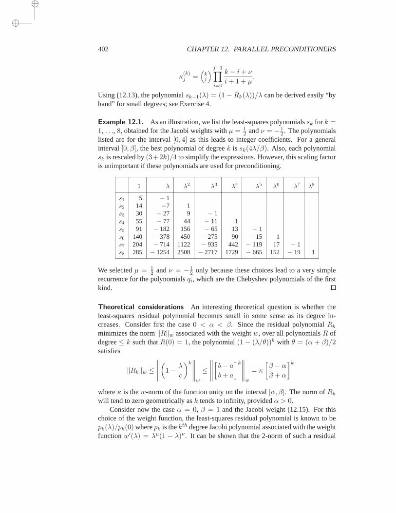
402 CHAPTER 12. PARALLEL PRECONDITIONERS
κ(k)j =
(kj
) j−1∏
i=0
k − i+ ν
i+ 1 + µ.
Using (12.13), the polynomialsk−1(λ) = (1− Rk(λ))/λ can be derived easily “byhand” for small degrees; see Exercise 4.
Example 12.1. As an illustration, we list the least-squares polynomialssk for k =1, . . ., 8, obtained for the Jacobi weights withµ = 1
2 andν = −12 . The polynomials
listed are for the interval[0, 4] as this leads to integer coefficients. For a generalinterval [0, β], the best polynomial of degreek is sk(4λ/β). Also, each polynomialsk is rescaled by(3+2k)/4 to simplify the expressions. However, this scaling factoris unimportant if these polynomials are used for preconditioning.
1 λ λ2 λ3 λ4 λ5 λ6 λ7 λ8
s1 5 − 1s2 14 −7 1s3 30 − 27 9 − 1s4 55 − 77 44 − 11 1s5 91 − 182 156 − 65 13 − 1s6 140 − 378 450 − 275 90 − 15 1s7 204 − 714 1122 − 935 442 − 119 17 − 1s8 285 − 1254 2508 − 2717 1729 − 665 152 − 19 1
We selectedµ = 12 andν = −1
2 only because these choices lead to a very simplerecurrence for the polynomialsqi, which are the Chebyshev polynomials of the firstkind.
Theoretical considerations An interesting theoretical question is whether theleast-squares residual polynomial becomes small in some sense as its degree in-creases. Consider first the case0 < α < β. Since the residual polynomialRk
minimizes the norm‖R‖w associated with the weightw, over all polynomialsR ofdegree≤ k such thatR(0) = 1, the polynomial(1 − (λ/θ))k with θ = (α + β)/2satisfies
‖Rk‖w ≤∥∥∥∥∥
(
1− λ
c
)k∥∥∥∥∥
w
≤∥∥∥∥∥
[b− ab+ a
]k∥∥∥∥∥
w
= κ
[β − αβ + α
]k
whereκ is thew-norm of the function unity on the interval[α, β]. The norm ofRk
will tend to zero geometrically ask tends to infinity, providedα > 0.Consider now the caseα = 0, β = 1 and the Jacobi weight (12.15). For this
choice of the weight function, the least-squares residual polynomial is known to bepk(λ)/pk(0) wherepk is thekth degree Jacobi polynomial associated with the weightfunctionw′(λ) = λµ(1 − λ)ν . It can be shown that the 2-norm of such a residual
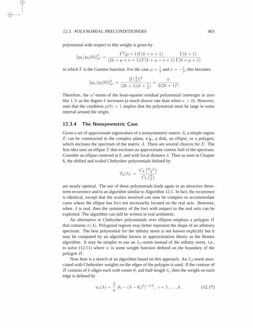
12.3. POLYNOMIAL PRECONDITIONERS 403
polynomial with respect to this weight is given by
‖pk/pk(0)‖2w′ =Γ2(µ+ 1)Γ(k + ν + 1)
(2k + µ+ ν + 1)(Γ(k + µ+ ν + 1)
Γ(k + 1)
Γ(k + µ+ 1)
in whichΓ is the Gamma function. For the caseµ = 12 andν = −1
2 , this becomes
‖pk/pk(0)‖2w′ =[Γ(3
2)]2
(2k + 1)(k + 12)
=π
2(2k + 1)2.
Therefore, thew′-norm of the least-squares residual polynomial converges to zerolike 1/k as the degreek increases (a much slower rate than whenα > 0). However,note that the conditionp(0) = 1 implies that the polynomial must be large in someinterval around the origin.
12.3.4 The Nonsymmetric Case
Given a set of approximate eigenvalues of a nonsymmetric matrixA, a simple regionE can be constructed in the complex plane, e.g., a disk, an ellipse, or a polygon,which encloses the spectrum of the matrixA. There are several choices forE. Thefirst idea uses an ellipseE that encloses an approximate convex hull of the spectrum.Consider an ellipse centered atθ, and with focal distanceδ. Then as seen in Chapter6, the shifted and scaled Chebyshev polynomials defined by
Tk(λ) =Ck
(θ−λ
δ
)
Ck
(θδ
)
are nearly optimal. The use of these polynomials leads again to an attractive three-term recurrence and to an algorithm similar to Algorithm 12.1. In fact, the recurrenceis identical, except that the scalars involved can now be complex to accommodatecases where the ellipse has foci not necessarily located on the real axis. However,whenA is real, then the symmetry of the foci with respect to the real axis can beexploited. The algorithm can still be written in real arithmetic.
An alternative to Chebyshev polynomials over ellipses employs a polygonHthat containsσ(A). Polygonal regions may better represent the shape of an arbitraryspectrum. The best polynomial for the infinity norm is not known explicitly butitmay be computed by an algorithm known in approximation theory as the Remezalgorithm. It may be simpler to use anL2-norm instead of the infinity norm, i.e.,to solve (12.11) wherew is some weight function defined on the boundary of thepolygonH.
Now here is a sketch of an algorithm based on this approach. AnL2-norm asso-ciated with Chebyshev weights on the edges of the polygon is used. If the contour ofH consists ofk edges each with centerθi and half-lengthδi, then the weight on eachedge is defined by
wi(λ) =2
π|δi − (λ− θi)
2|−1/2, i = 1, . . . , k. (12.17)
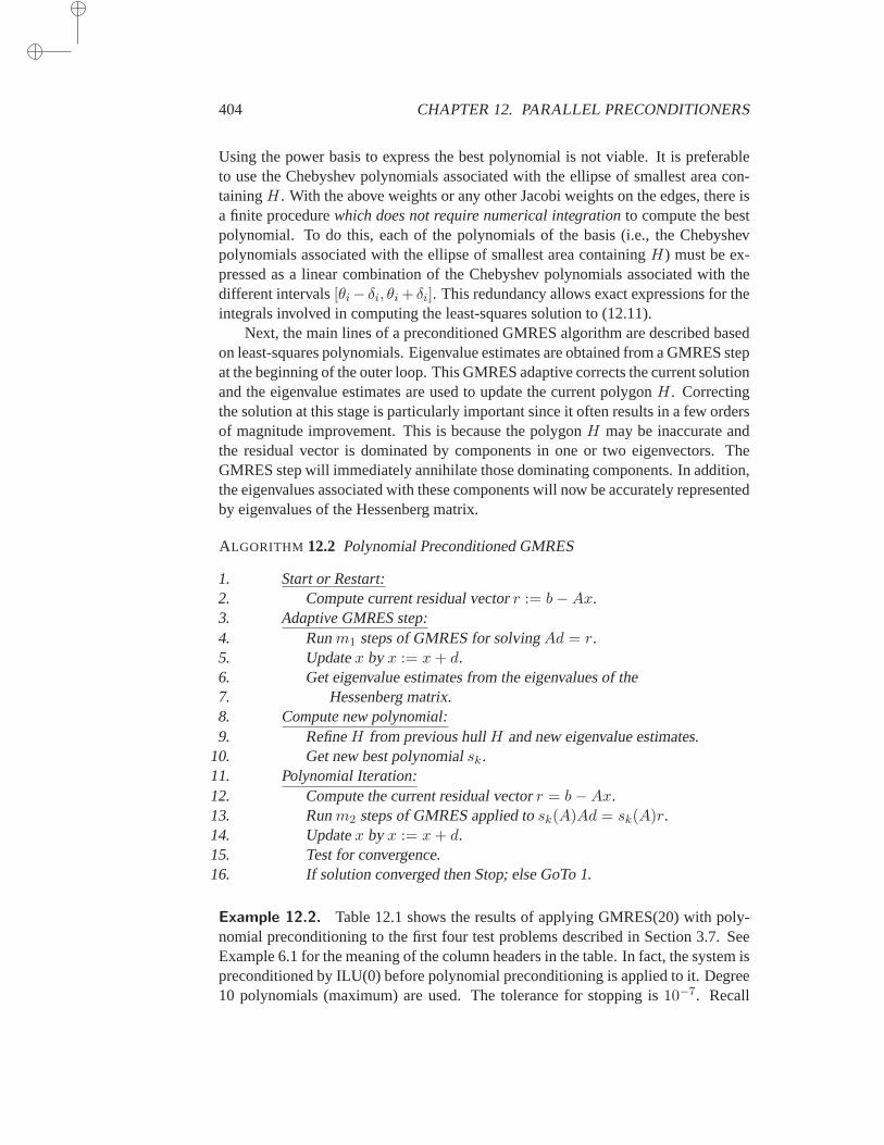
404 CHAPTER 12. PARALLEL PRECONDITIONERS
Using the power basis to express the best polynomial is not viable. It is preferableto use the Chebyshev polynomials associated with the ellipse of smallest area con-tainingH. With the above weights or any other Jacobi weights on the edges, there isa finite procedurewhich does not require numerical integrationto compute the bestpolynomial. To do this, each of the polynomials of the basis (i.e., the Chebyshevpolynomials associated with the ellipse of smallest area containingH) must be ex-pressed as a linear combination of the Chebyshev polynomials associated withthedifferent intervals[θi− δi, θi + δi]. This redundancy allows exact expressions for theintegrals involved in computing the least-squares solution to (12.11).
Next, the main lines of a preconditioned GMRES algorithm are described basedon least-squares polynomials. Eigenvalue estimates are obtained from a GMRES stepat the beginning of the outer loop. This GMRES adaptive corrects the current solutionand the eigenvalue estimates are used to update the current polygonH. Correctingthe solution at this stage is particularly important since it often results in a few ordersof magnitude improvement. This is because the polygonH may be inaccurate andthe residual vector is dominated by components in one or two eigenvectors. TheGMRES step will immediately annihilate those dominating components. In addition,the eigenvalues associated with these components will now be accurately representedby eigenvalues of the Hessenberg matrix.
ALGORITHM 12.2 Polynomial Preconditioned GMRES
1. Start or Restart:2. Compute current residual vectorr := b−Ax.3. Adaptive GMRES step:4. Runm1 steps of GMRES for solvingAd = r.5. Updatex by x := x+ d.6. Get eigenvalue estimates from the eigenvalues of the7. Hessenberg matrix.8. Compute new polynomial:9. RefineH from previous hullH and new eigenvalue estimates.
10. Get new best polynomialsk.11. Polynomial Iteration:12. Compute the current residual vectorr = b−Ax.13. Runm2 steps of GMRES applied tosk(A)Ad = sk(A)r.14. Updatex by x := x+ d.15. Test for convergence.16. If solution converged then Stop; else GoTo 1.
Example 12.2. Table 12.1 shows the results of applying GMRES(20) with poly-nomial preconditioning to the first four test problems described in Section 3.7. SeeExample 6.1 for the meaning of the column headers in the table. In fact, the system ispreconditioned by ILU(0) before polynomial preconditioning is applied to it.Degree10 polynomials (maximum) are used. The tolerance for stopping is10−7. Recall
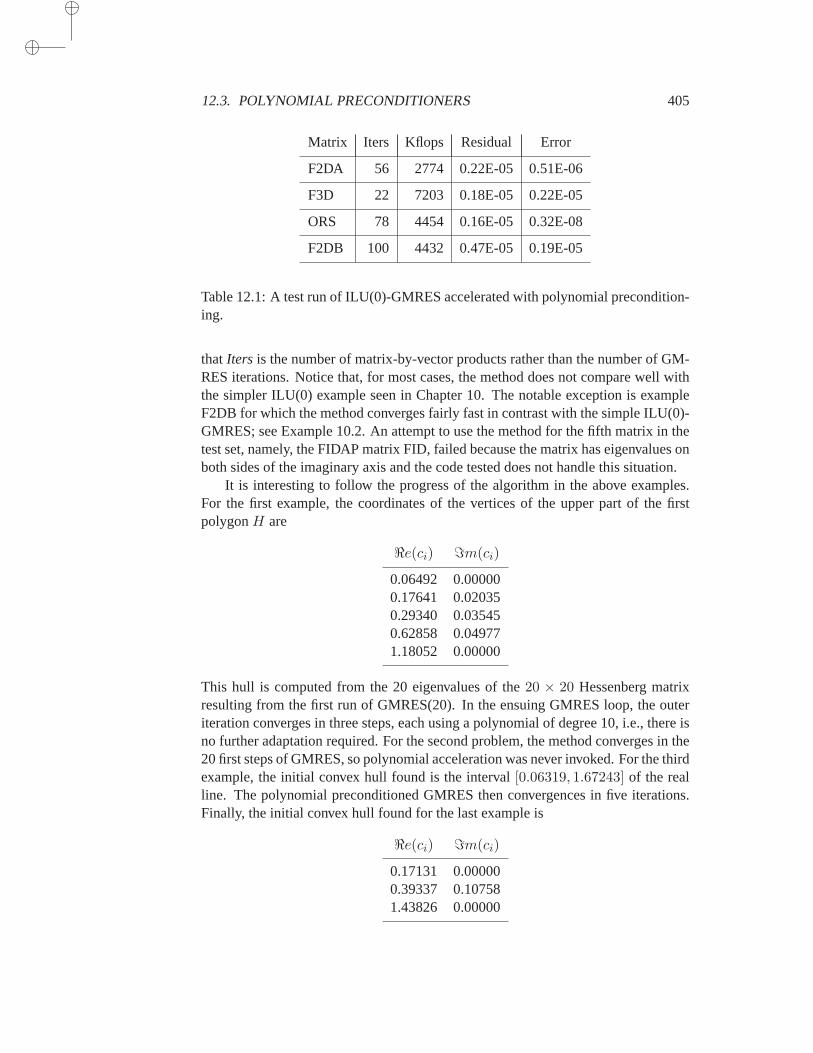
12.3. POLYNOMIAL PRECONDITIONERS 405
Matrix Iters Kflops Residual Error
F2DA 56 2774 0.22E-05 0.51E-06
F3D 22 7203 0.18E-05 0.22E-05
ORS 78 4454 0.16E-05 0.32E-08
F2DB 100 4432 0.47E-05 0.19E-05
Table 12.1: A test run of ILU(0)-GMRES accelerated with polynomial precondition-ing.
thatIters is the number of matrix-by-vector products rather than the number of GM-RES iterations. Notice that, for most cases, the method does not compare wellwiththe simpler ILU(0) example seen in Chapter 10. The notable exception is exampleF2DB for which the method converges fairly fast in contrast with the simple ILU(0)-GMRES; see Example 10.2. An attempt to use the method for the fifth matrix in thetest set, namely, the FIDAP matrix FID, failed because the matrix has eigenvalues onboth sides of the imaginary axis and the code tested does not handle this situation.
It is interesting to follow the progress of the algorithm in the above examples.For the first example, the coordinates of the vertices of the upper part ofthe firstpolygonH are
ℜe(ci) ℑm(ci)
0.06492 0.000000.17641 0.020350.29340 0.035450.62858 0.049771.18052 0.00000
This hull is computed from the 20 eigenvalues of the20 × 20 Hessenberg matrixresulting from the first run of GMRES(20). In the ensuing GMRES loop, the outeriteration converges in three steps, each using a polynomial of degree 10,i.e., there isno further adaptation required. For the second problem, the method converges in the20 first steps of GMRES, so polynomial acceleration was never invoked.For the thirdexample, the initial convex hull found is the interval[0.06319, 1.67243] of the realline. The polynomial preconditioned GMRES then convergences in five iterations.Finally, the initial convex hull found for the last example is
ℜe(ci) ℑm(ci)
0.17131 0.000000.39337 0.107581.43826 0.00000
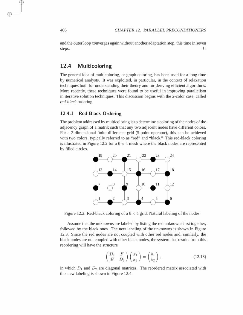
406 CHAPTER 12. PARALLEL PRECONDITIONERS
and the outer loop converges again without another adaptation step, this time insevensteps.
12.4 Multicoloring
The general idea of multicoloring, or graph coloring, has been used fora long timeby numerical analysts. It was exploited, in particular, in the context of relaxationtechniques both for understanding their theory and for deriving efficient algorithms.More recently, these techniques were found to be useful in improving parallelismin iterative solution techniques. This discussion begins with the 2-color case, calledred-blackordering.
12.4.1 Red-Black Ordering
The problem addressed by multicoloring is to determine a coloring of the nodesof theadjacency graph of a matrix such that any two adjacent nodes have different colors.For a 2-dimensional finite difference grid (5-point operator), this can be achievedwith two colors, typically referred to as “red” and “black.” This red-black coloringis illustrated in Figure 12.2 for a6 × 4 mesh where the black nodes are representedby filled circles.
1 3 5
8 10 12
13 15 17
20 22 24
2 4 6
7 9 11
14 16 18
19 21 23
Figure 12.2: Red-black coloring of a6× 4 grid. Natural labeling of the nodes.
Assume that the unknowns are labeled by listing the red unknowns first together,followed by the black ones. The new labeling of the unknowns is shown in Figure12.3. Since the red nodes are not coupled with other red nodes and, similarly, theblack nodes are not coupled with other black nodes, the system that results from thisreordering will have the structure
(D1 FE D2
)(x1
x2
)
=
(b1b2
)
, (12.18)
in whichD1 andD2 are diagonal matrices. The reordered matrix associated withthis new labeling is shown in Figure 12.4.
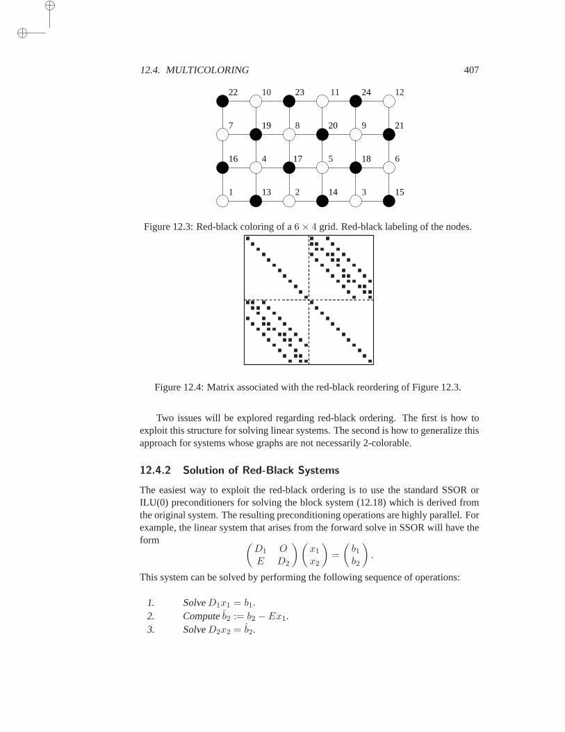
12.4. MULTICOLORING 407
1 2 3
4 5 6
7 8 9
10 11 12
13 14 15
16 17 18
19 20 21
22 23 24
Figure 12.3: Red-black coloring of a6× 4 grid. Red-black labeling of the nodes.
Figure 12.4: Matrix associated with the red-black reordering of Figure 12.3.
Two issues will be explored regarding red-black ordering. The first ishow toexploit this structure for solving linear systems. The second is how to generalize thisapproach for systems whose graphs are not necessarily 2-colorable.
12.4.2 Solution of Red-Black Systems
The easiest way to exploit the red-black ordering is to use the standard SSOR orILU(0) preconditioners for solving the block system (12.18) which is derived fromthe original system. The resulting preconditioning operations are highly parallel. Forexample, the linear system that arises from the forward solve in SSOR will have theform (
D1 OE D2
)(x1
x2
)
=
(b1b2
)
.
This system can be solved by performing the following sequence of operations:
1. SolveD1x1 = b1.2. Computeb2 := b2 − Ex1.3. SolveD2x2 = b2.
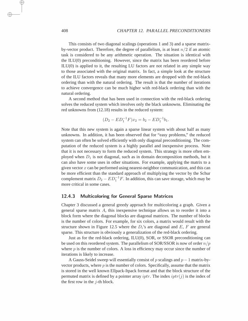
408 CHAPTER 12. PARALLEL PRECONDITIONERS
This consists of two diagonal scalings (operations 1 and 3) and a sparsematrix-by-vector product. Therefore, the degree of parallelism, is at leastn/2 if an atomictask is considered to be any arithmetic operation. The situation is identical withthe ILU(0) preconditioning. However, since the matrix has been reordered beforeILU(0) is applied to it, the resulting LU factors are not related in any simple wayto those associated with the original matrix. In fact, a simple look at the structureof the ILU factors reveals that many more elements are dropped with the red-blackordering than with the natural ordering. The result is that the number of iterationsto achieve convergence can be much higher with red-black ordering thanwith thenatural ordering.
A second method that has been used in connection with the red-black orderingsolves the reduced system which involves only the black unknowns. Eliminating thered unknowns from (12.18) results in the reduced system:
(D2 − ED−11 F )x2 = b2 − ED−1
1 b1.
Note that this new system is again a sparse linear system with about half as manyunknowns. In addition, it has been observed that for “easy problems,” the reducedsystem can often be solved efficiently with only diagonal preconditioning. The com-putation of the reduced system is a highly parallel and inexpensive process. Notethat it is not necessary to form the reduced system. This strategy is more often em-ployed whenD1 is not diagonal, such as in domain decomposition methods, but itcan also have some uses in other situations. For example, applying the matrix to agiven vectorx can be performed using nearest-neighbor communication, and this canbe more efficient than the standard approach of multiplying the vector by the Schurcomplement matrixD2 −ED−1
1 F . In addition, this can save storage, which may bemore critical in some cases.
12.4.3 Multicoloring for General Sparse Matrices
Chapter 3 discussed a general greedy approach for multicoloring a graph. Given ageneral sparse matrixA, this inexpensive technique allows us to reorder it into ablock form where the diagonal blocks are diagonal matrices. The numberof blocksis the number of colors. For example, for six colors, a matrix would result withthestructure shown in Figure 12.5 where theDi’s are diagonal andE, F are generalsparse. This structure is obviously a generalization of the red-black ordering.
Just as for the red-black ordering, ILU(0), SOR, or SSOR preconditioning canbe used on this reordered system. The parallelism of SOR/SSOR is now of ordern/pwherep is the number of colors. A loss in efficiency may occur since the number ofiterations is likely to increase.
A Gauss-Seidel sweep will essentially consist ofp scalings andp− 1 matrix-by-vector products, wherep is the number of colors. Specifically, assume that the matrixis stored in the well known Ellpack-Itpack format and that the block structure of thepermuted matrix is defined by a pointer arrayiptr. The indexiptr(j) is the index ofthe first row in thej-th block.
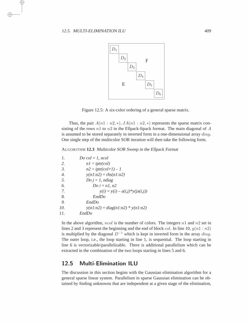
12.5. MULTI-ELIMINATION ILU 409
D1
D2
D3
D4
D5
D6
F
E
Figure 12.5: A six-color ordering of a general sparse matrix.
Thus, the pairA(n1 : n2, ∗), JA(n1 : n2, ∗) represents the sparse matrix con-sisting of the rowsn1 to n2 in the Ellpack-Itpack format. The main diagonal ofAis assumed to be stored separately in inverted form in a one-dimensional arraydiag.One single step of the multicolor SOR iteration will then take the following form.
ALGORITHM 12.3 Multicolor SOR Sweep in the Ellpack Format
1. Do col = 1, ncol2. n1 = iptr(col)3. n2 = iptr(col+1) – 14. y(n1:n2) = rhs(n1:n2)5. Do j = 1, ndiag6. Do i = n1, n27. y(i) = y(i) – a(i,j)*y(ja(i,j))8. EndDo9. EndDo
10. y(n1:n2) = diag(n1:n2) * y(n1:n2)11. EndDo
In the above algorithm,ncol is the number of colors. The integersn1 andn2 set inlines 2 and 3 represent the beginning and the end of blockcol. In line 10,y(n1 : n2)is multiplied by the diagonalD−1 which is kept in inverted form in the arraydiag.The outer loop, i.e., the loop starting in line 1, is sequential. The loop starting inline 6 is vectorizable/parallelizable. There is additional parallelism which can beextracted in the combination of the two loops starting in lines 5 and 6.
12.5 Multi-Elimination ILU
The discussion in this section begins with the Gaussian elimination algorithm for ageneral sparse linear system. Parallelism in sparse Gaussian elimination canbe ob-tained by finding unknowns that are independent at a given stage of theelimination,
410 CHAPTER 12. PARALLEL PRECONDITIONERS
i.e., unknowns that do not depend on each other according to the binary relation de-fined by the graph of the matrix. A set of unknowns of a linear system whichareindependent is called an independent set. Thus, independent set orderings can beviewed as permutations to put the original matrix in the form
(D EF C
)
(12.19)
in whichD is diagonal, butC can be arbitrary. This amounts to a less restrictiveform of multicoloring, in which a set of vertices in the adjacency graph is found sothat no equation in the set involves unknowns from the same set. A few algorithmsfor finding independent set orderings of a general sparse graph were discussed inChapter 3.
The rows associated with an independent set can be used as pivots simultane-ously. When such rows are eliminated, a smaller linear system results, which isagainsparse. Then we can find an independent set for this reduced systemand repeat theprocess of reduction. The resulting second reduced system is called thesecond-levelreduced system.
The process can be repeated recursively a few times. As the level of thereduc-tion increases, the reduced systems gradually lose their sparsity. A directsolutionmethod would continue the reduction until the reduced system is small enough ordense enough to switch to a dense Gaussian elimination to solve it. This processisillustrated in Figure 12.6. There exists a number of sparse direct solution techniquesbased on this approach.
Figure 12.6: Illustration of two levels of multi-elimination for sparse linear systems.
After a brief review of the direct solution method based on independent set or-derings, we will explain how to exploit this approach for deriving incompleteLUfactorizations by incorporating drop tolerance strategies.
12.5.1 Multi-Elimination
We start by a discussion of anexactreduction step. LetAj be the matrix obtainedat thej-th step of the reduction,j = 0, . . . , nlev with A0 = A. Assume that anindependent set ordering is applied toAj and that the matrix is permuted accordingly
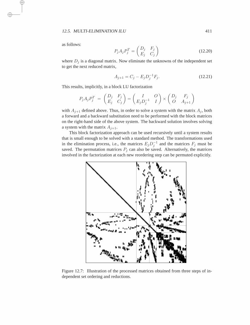
12.5. MULTI-ELIMINATION ILU 411
as follows:
PjAjPTj =
(Dj Fj
Ej Cj
)
(12.20)
whereDj is a diagonal matrix. Now eliminate the unknowns of the independent setto get the next reduced matrix,
Aj+1 = Cj − EjD−1j Fj . (12.21)
This results, implicitly, in a block LU factorization
PjAjPTj =
(Dj Fj
Ej Cj
)
=
(I O
EjD−1j I
)
×(Dj Fj
O Aj+1
)
with Aj+1 defined above. Thus, in order to solve a system with the matrixAj , botha forward and a backward substitution need to be performed with the block matriceson the right-hand side of the above system. The backward solution involvessolvinga system with the matrixAj+1.
This block factorization approach can be used recursively until a system resultsthat is small enough to be solved with a standard method. The transformations usedin the elimination process, i.e., the matricesEjD
−1j and the matricesFj must be
saved. The permutation matricesPj can also be saved. Alternatively, the matricesinvolved in the factorization at each new reordering step can be permuted explicitly.
Figure 12.7: Illustration of the processed matrices obtained from three steps of in-dependent set ordering and reductions.
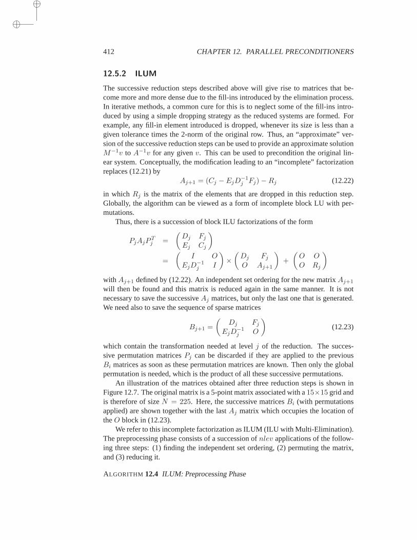
412 CHAPTER 12. PARALLEL PRECONDITIONERS
12.5.2 ILUM
The successive reduction steps described above will give rise to matrices that be-come more and more dense due to the fill-ins introduced by the elimination process.In iterative methods, a common cure for this is to neglect some of the fill-ins intro-duced by using a simple dropping strategy as the reduced systems are formed. Forexample, any fill-in element introduced is dropped, whenever its size is less than agiven tolerance times the 2-norm of the original row. Thus, an “approximate” ver-sion of the successive reduction steps can be used to provide an approximate solutionM−1v to A−1v for any givenv. This can be used to precondition the original lin-ear system. Conceptually, the modification leading to an “incomplete” factorizationreplaces (12.21) by
Aj+1 = (Cj − EjD−1j Fj)−Rj (12.22)
in which Rj is the matrix of the elements that are dropped in this reduction step.Globally, the algorithm can be viewed as a form of incomplete block LU with per-mutations.
Thus, there is a succession of block ILU factorizations of the form
PjAjPTj =
(Dj Fj
Ej Cj
)
=
(I O
EjD−1j I
)
×(Dj Fj
O Aj+1
)
+
(O OO Rj
)
with Aj+1 defined by (12.22). An independent set ordering for the new matrixAj+1
will then be found and this matrix is reduced again in the same manner. It is notnecessary to save the successiveAj matrices, but only the last one that is generated.We need also to save the sequence of sparse matrices
Bj+1 =
(Dj Fj
EjD−1j O
)
(12.23)
which contain the transformation needed at levelj of the reduction. The succes-sive permutation matricesPj can be discarded if they are applied to the previousBi matrices as soon as these permutation matrices are known. Then only the globalpermutation is needed, which is the product of all these successive permutations.
An illustration of the matrices obtained after three reduction steps is shown inFigure 12.7. The original matrix is a 5-point matrix associated with a15×15 grid andis therefore of sizeN = 225. Here, the successive matricesBi (with permutationsapplied) are shown together with the lastAj matrix which occupies the location oftheO block in (12.23).
We refer to this incomplete factorization as ILUM (ILU with Multi-Elimination).The preprocessing phase consists of a succession ofnlev applications of the follow-ing three steps: (1) finding the independent set ordering, (2) permutingthe matrix,and (3) reducing it.
ALGORITHM 12.4 ILUM: Preprocessing Phase
12.5. MULTI-ELIMINATION ILU 413
1. SetA0 = A.2. Forj = 0, 1, . . . , nlev − 1 Do:3. Find an independent set ordering permutationPj for Aj ;4. ApplyPj toAj to permute it into the form (12.20);5. ApplyPj toB1, . . . , Bj ;6. ApplyPj to P0, . . . , Pj−1;7. Compute the matricesAj+1 andBj+1 defined by (12.22) and (12.23).8. EndDo
In the backward and forward solution phases, the last reduced systemmust be solvedbut not necessarily with high accuracy. For example, we can solve it according to thelevel of tolerance allowed in the dropping strategy during the preprocessing phase.
Observe that if the linear system is solved inaccurately, only an accelerator thatallows variations in the preconditioning should be used. Such algorithms have beendiscussed in Chapter 9. Alternatively, we can use a fixed number of multicolor SORor SSOR steps or a fixed polynomial iteration. The implementation of the ILUM pre-conditioner corresponding to this strategy is rather complicated and involvesseveralparameters.
In order to describe the forward and backward solution, we introduce some no-tation. We start by applying the “global permutation,” i.e., the product
Pnlev−1, Pnlev−2 . . . , P0
to the right-hand side. We overwrite the result on the current solution vector, anN -vector calledx0. Now partition this vector into
x0 =
(y0
x1
)
according to the partitioning (12.20). The forward step consists of transforming thesecond component of the right-hand side as
x1 := x1 − E0D−10 y0.
Now x1 is partitioned in the same manner asx0 and the forward elimination is con-tinued the same way. Thus, at each step, eachxj is partitioned as
xj =
(yj
xj+1
)
.
A forward elimination step defines the newxj+1 using the oldxj+1 andyj for j =0, . . . , nlev − 1 while a backward step definesyj using the oldyj andxj+1, forj = nlev − 1, . . . , 0. Algorithm 12.5 describes the general structure of the forwardand backward solution sweeps. Because the global permutation was applied at thebeginning, the successive permutations need not be applied. However,the final resultobtained must be permuted back into the original ordering.

414 CHAPTER 12. PARALLEL PRECONDITIONERS
ALGORITHM 12.5 ILUM: Forward and Backward Solutions
1. Apply global permutation to right-hand-sideb and copy intox0.2. Forj = 0, 1, . . . , nlev − 1 Do: [Forward sweep]3. xj+1 := xj+1 − EjD
−1j yj
4. EndDo5. Solve with a relative toleranceǫ:6. Anlevxnlev := xnlev.7. Forj = nlev − 1, . . . , 1, 0 Do: [Backward sweep]8. yj := D−1
j (yj − Fjxj+1).9. EndDo
10. Permute the resulting solution vector back to the original11. ordering to obtain the solutionx.
Computer implementations of ILUM can be rather tedious. The implementa-tion issues are similar to those of parallel direct-solution methods for sparse linearsystems.
12.6 Distributed ILU and SSOR
This section describes parallel variants of the block Successive Over-Relaxation(BSOR) and ILU(0) preconditioners which are suitable for distributed memory en-vironments. Chapter 11 briefly discusseddistributed sparse matrices. A distributedmatrix is a matrix whose entries are located in the memories of different processorsin a multiprocessor system. These types of data structures are very convenient fordistributed memory computers and it is useful to discuss implementations of precon-ditioners that are specifically developed for them. Refer to Section 11.5.5 for theterminology used here. In particular, the termsubdomainis used in the very generalsense of subgraph. For both ILU and SOR, multicoloring or level scheduling can beused at the macro level, to extract parallelism. Here, macro level means the level ofparallelism corresponding to the processors, or blocks, or subdomains.
In the ILU(0) factorization, the LU factors have the same nonzero patterns asthe original matrixA, so that the references of the entries belonging to the externalsubdomains in the ILU(0) factorization are identical with those of the matrix-by-vector product operation with the matrixA. This is not the case for the more accurateILU(p) factorization, withp > 0. If an attempt is made to implement a wavefrontILU preconditioner on a distributed memory computer, a difficulty arises because thenatural ordering for the original sparse problem may put an unnecessary limit on theamount of parallelism available. Instead, a two-level ordering is used. First, define a“global” ordering which is a wavefront ordering for the subdomains. This is based onthe graph which describes the coupling between the subdomains: Two subdomainsare coupled if and only if they contain at least a pair of coupled unknowns, one fromeach subdomain. Then, within each subdomain, define a local ordering.
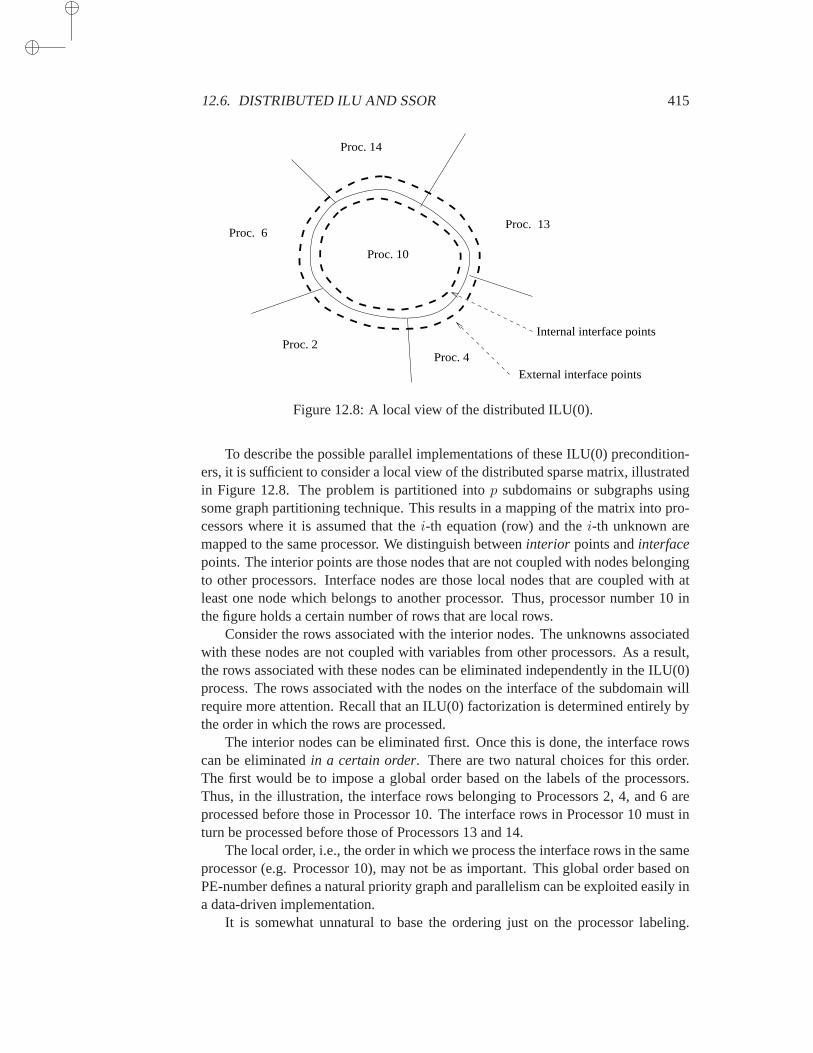
12.6. DISTRIBUTED ILU AND SSOR 415
Internal interface points
External interface points
Proc. 2 Proc. 4
Proc. 6
Proc. 14
Proc. 13
Proc. 10
Figure 12.8: A local view of the distributed ILU(0).
To describe the possible parallel implementations of these ILU(0) precondition-ers, it is sufficient to consider a local view of the distributed sparse matrix,illustratedin Figure 12.8. The problem is partitioned intop subdomains or subgraphs usingsome graph partitioning technique. This results in a mapping of the matrix into pro-cessors where it is assumed that thei-th equation (row) and thei-th unknown aremapped to the same processor. We distinguish betweeninterior points andinterfacepoints. The interior points are those nodes that are not coupled with nodesbelongingto other processors. Interface nodes are those local nodes that arecoupled with atleast one node which belongs to another processor. Thus, processor number 10 inthe figure holds a certain number of rows that are local rows.
Consider the rows associated with the interior nodes. The unknowns associatedwith these nodes are not coupled with variables from other processors.As a result,the rows associated with these nodes can be eliminated independently in the ILU(0)process. The rows associated with the nodes on the interface of the subdomain willrequire more attention. Recall that an ILU(0) factorization is determined entirely bythe order in which the rows are processed.
The interior nodes can be eliminated first. Once this is done, the interface rowscan be eliminatedin a certain order. There are two natural choices for this order.The first would be to impose a global order based on the labels of the processors.Thus, in the illustration, the interface rows belonging to Processors 2, 4, and 6 areprocessed before those in Processor 10. The interface rows in Processor 10 must inturn be processed before those of Processors 13 and 14.
The local order, i.e., the order in which we process the interface rows in the sameprocessor (e.g. Processor 10), may not be as important. This global order based onPE-number defines a natural priority graph and parallelism can be exploited easily ina data-driven implementation.
It is somewhat unnatural to base the ordering just on the processor labeling.
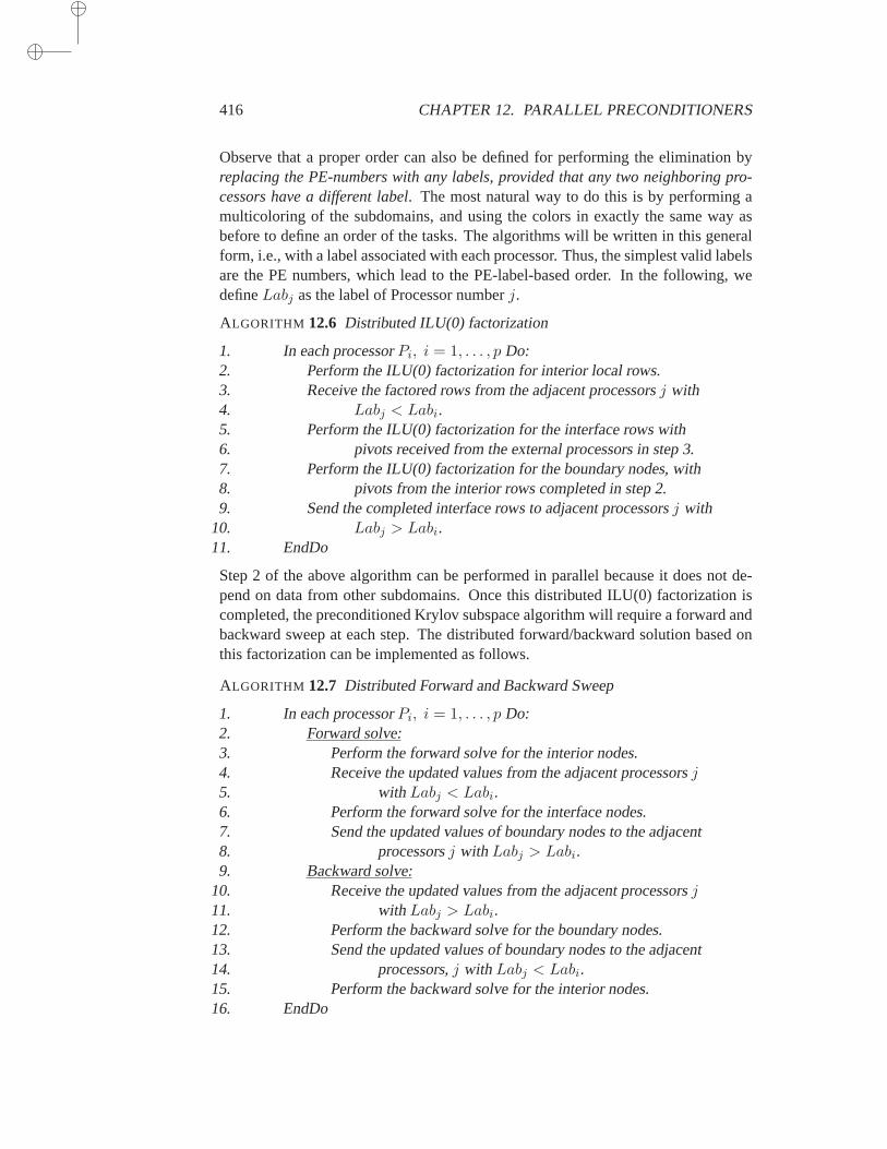
416 CHAPTER 12. PARALLEL PRECONDITIONERS
Observe that a proper order can also be defined for performing the elimination byreplacing the PE-numbers with any labels, provided that any two neighboring pro-cessors have a different label. The most natural way to do this is by performing amulticoloring of the subdomains, and using the colors in exactly the same way asbefore to define an order of the tasks. The algorithms will be written in this generalform, i.e., with a label associated with each processor. Thus, the simplest valid labelsare the PE numbers, which lead to the PE-label-based order. In the following, wedefineLabj as the label of Processor numberj.
ALGORITHM 12.6 Distributed ILU(0) factorization
1. In each processorPi, i = 1, . . . , p Do:2. Perform the ILU(0) factorization for interior local rows.3. Receive the factored rows from the adjacent processorsj with4. Labj < Labi.5. Perform the ILU(0) factorization for the interface rows with6. pivots received from the external processors in step 3.7. Perform the ILU(0) factorization for the boundary nodes, with8. pivots from the interior rows completed in step 2.9. Send the completed interface rows to adjacent processorsj with
10. Labj > Labi.11. EndDo
Step 2 of the above algorithm can be performed in parallel because it doesnot de-pend on data from other subdomains. Once this distributed ILU(0) factorization iscompleted, the preconditioned Krylov subspace algorithm will require a forward andbackward sweep at each step. The distributed forward/backward solution based onthis factorization can be implemented as follows.
ALGORITHM 12.7 Distributed Forward and Backward Sweep
1. In each processorPi, i = 1, . . . , p Do:2. Forward solve:3. Perform the forward solve for the interior nodes.4. Receive the updated values from the adjacent processorsj5. withLabj < Labi.6. Perform the forward solve for the interface nodes.7. Send the updated values of boundary nodes to the adjacent8. processorsj with Labj > Labi.9. Backward solve:
10. Receive the updated values from the adjacent processorsj11. withLabj > Labi.12. Perform the backward solve for the boundary nodes.13. Send the updated values of boundary nodes to the adjacent14. processors,j with Labj < Labi.15. Perform the backward solve for the interior nodes.16. EndDo
12.7. OTHER TECHNIQUES 417
As in the ILU(0) factorization, the interior nodes do not depend on the nodes fromthe external processors and can be computed in parallel in lines 3 and 15.In theforward solve, the solution of the interior nodes is followed by an exchange of dataand the solution on the interface. The backward solve works in reverse inthat theboundary nodes are first computed, then they are sent to adjacent processors. Finally,interior nodes are updated.
12.7 Other Techniques
This section gives a brief account of other parallel preconditioning techniques whichare sometimes used. The next chapter also examines another important classof meth-ods, which were briefly mentioned before, namely, the class of Domain Decomposi-tion methods.
12.7.1 Approximate Inverses
Another class of preconditioners that require only matrix-by-vector products, is theclass of approximate inverse preconditioners. Discussed in Chapter 10,these can beused in many different ways. Besides being simple to implement, both their prepro-cessing phase and iteration phase allow a large degree of parallelism. Theirdisadvan-tage is similar to polynomial preconditioners, namely, the number of steps requiredfor convergence may be large, possibly substantially larger than with the standardtechniques. On the positive side, they are fairly robust techniques whichcan workwell where standard methods may fail.
12.7.2 Element-by-Element Techniques
A somewhat specialized set of techniques is the class of Element-By-Element(EBE)preconditioners which are geared toward finite element problems and are motivatedby the desire to avoid assembling finite element matrices. Many finite element codeskeep the data related to the linear system in unassembled form. The element matricesassociated with each element are stored and never added together. This isconvenientwhen using direct methods since there are techniques, known as frontalmethods, thatallow Gaussian elimination to be performed by using a few elements at a time.
It was seen in Chapter 2 that the global stiffness matrixA is the sum of matricesA[e] associated with each element, i.e.,
A =Nel∑
e=1
A[e].
Here, the matrixA[e] is ann× n matrix defined as
A[e] = PeAKePTe
in whichAKe is the element matrix andPe is a Boolean connectivity matrix whichmaps the coordinates of the smallAKe matrix into those of the full matrixA. Chapter
418 CHAPTER 12. PARALLEL PRECONDITIONERS
2 showed how matrix-by-vector products can be performed in unassembled form. Toperform this product in parallel, note that the only potential obstacle to performingthe matrix-by-vector product in parallel, i.e., across all elements, is in the lastphase,i.e., when the contributions are summed to the resulting vectory. In order to add thecontributionsA[e]x in parallel, group elements that do not have nodes in common.Referring to Equation (2.46), the contributions
ye = AKe(PTe x)
can all be computed in parallel and do not depend on one another. The operations
y := y + Peye
can be processed in parallel for any group of elements that do not share any vertices.This grouping can be found by performing a multicoloring of the elements. Anytwoelements which have a node in common receive a different color. Using this idea,good performance can be achieved on vector computers.
EBE preconditioners are based on similar principles and many different variantshave been developed. They are defined by first normalizing each of theelementmatrices. In the sequel, assume thatA is a Symmetric Positive Definite matrix.Typically, a diagonal, or block diagonal, scaling is first applied toA to obtain ascaled matrixA,
A = D−1/2AD−1/2. (12.24)
This results in each matrixA[e] and element matrixAKe being transformed similarly:
A[e] = D−1/2A[e]D−1/2
= D−1/2PeAKeD−1/2
= Pe(PTe D
−1/2Pe)A[e](PeD
−1/2P Te )
≡ PeAKePTe .
The second step in defining an EBE preconditioner is toregularizeeach of thesetransformed matrices. Indeed, each of the matricesA[e] is of rankpe at most, wherepe is the size of the element matrixAKe , i.e., the number of nodes which constitutethee-th element. In the so-calledWinget regularization, the diagonal of eachA[e] isforced to be the identity matrix. In other words, the regularized matrix is defined as
A[e] = I + A[e] − diag(A[e]). (12.25)
These matrices are positive definite; see Exercise 8.The third and final step in defining an EBE preconditioner is to choose the fac-
torization itself. In the EBE Cholesky factorization, the Cholesky (or Crout)factor-ization of each regularized matrixA[e] is performed,
A[e] = LeDeLTe . (12.26)
12.7. OTHER TECHNIQUES 419
The preconditioner from it is defined as
M =nel∏
e=1
Le ×nel∏
e=1
De ×1∏
e=nel
LTe . (12.27)
Note that to ensure symmetry, the last product is in reverse order of the first one.The factorization (12.26) consists of a factorization of the smallpe× pe matrix AKe .Performing the preconditioning operations will therefore consist of a sequence ofsmallpe×pe backward or forward solves. The gather and scatter matricesPe definedin Chapter 2 must also be applied for each element. These solves are appliedtothe right-hand side in sequence. In addition, the same multicoloring idea as forthematrix-by-vector product can be exploited to perform these sweeps in parallel.
One of the drawbacks of the EBE Cholesky preconditioner is that an additionalset of element matrices must be stored. That is because the factorizations (12.26)must be stored for each element. In EBE/SSOR, this is avoided. Instead of factor-ing eachA[e], the usual splitting of eachA[e] is exploited. Assuming the Wingetregularization, we have
A[e] = I − Ee − ETe (12.28)
in which−Ee is the strict-lower part ofA[e]. By analogy with the SSOR precondi-tioner, the EBE-SSOR preconditioner is defined by
M =nel∏
e=1
(I − ωEe)×nel∏
e=1
De ×1∏
e=nel
(I − ωETe ). (12.29)
12.7.3 Parallel Row Projection Preconditioners
One of the attractions of row-projection methods seen in Chapter 8 is their highde-gree of parallelism. In Cimmino’s method, the scalarsδi as well as the new residualvector can be computed in parallel. In the Gauss-Seidel-NE (respectivelyGauss-Seidel-NR), it is also possible to group the unknowns in such a way that anypairof rows (respectively columns) have disjointed nonzero patterns. Updates of com-ponents in the same group can then be performed in parallel. This approachessen-tially requires finding a multicolor ordering for the matrixB = AAT (respectivelyB = ATA ).
It is necessary to first identify a partition of the set1, 2, . . . , N into subsetsS1, . . ., Sk such that the rows (respectively columns) whose indices belong to thesame setSi arestructurallyorthogonal to each other, i.e., have no nonzero elementsin the same column locations. When implementing a block SOR scheme where theblocking is identical with that defined by the partition, all of the unknowns belongingto the same setSj can be updated in parallel. To be more specific, the rows arereordered by scanning those inS1 followed by those inS2, etc.. Denote byAi thematrix consisting of the rows belonging to thei-th block. We assume that all rowsof the same set are orthogonal to each other and that they have been normalized
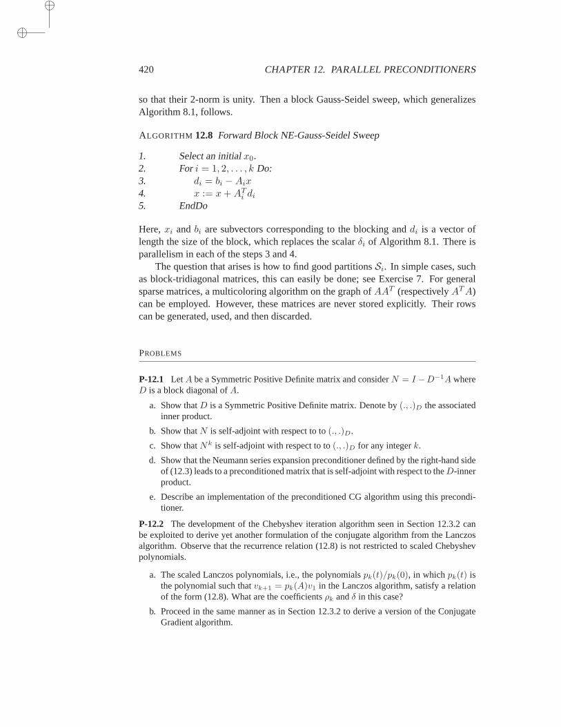
420 CHAPTER 12. PARALLEL PRECONDITIONERS
so that their 2-norm is unity. Then a block Gauss-Seidel sweep, which generalizesAlgorithm 8.1, follows.
ALGORITHM 12.8 Forward Block NE-Gauss-Seidel Sweep
1. Select an initialx0.2. Fori = 1, 2, . . . , k Do:3. di = bi −Aix4. x := x+AT
i di
5. EndDo
Here,xi andbi are subvectors corresponding to the blocking anddi is a vector oflength the size of the block, which replaces the scalarδi of Algorithm 8.1. There isparallelism in each of the steps 3 and 4.
The question that arises is how to find good partitionsSi. In simple cases, suchas block-tridiagonal matrices, this can easily be done; see Exercise 7. For generalsparse matrices, a multicoloring algorithm on the graph ofAAT (respectivelyATA)can be employed. However, these matrices are never stored explicitly. Their rowscan be generated, used, and then discarded.
PROBLEMS
P-12.1 LetA be a Symmetric Positive Definite matrix and considerN = I −D−1A whereD is a block diagonal ofA.
a. Show thatD is a Symmetric Positive Definite matrix. Denote by(., .)D the associatedinner product.
b. Show thatN is self-adjoint with respect to to(., .)D.
c. Show thatNk is self-adjoint with respect to to(., .)D for any integerk.
d. Show that the Neumann series expansion preconditioner defined by the right-hand sideof (12.3) leads to a preconditioned matrix that is self-adjoint with respect to theD-innerproduct.
e. Describe an implementation of the preconditioned CG algorithm using this precondi-tioner.
P-12.2 The development of the Chebyshev iteration algorithm seen in Section 12.3.2 canbe exploited to derive yet another formulation of the conjugate algorithm from the Lanczosalgorithm. Observe that the recurrence relation (12.8) is not restricted to scaled Chebyshevpolynomials.
a. The scaled Lanczos polynomials, i.e., the polynomialspk(t)/pk(0), in whichpk(t) isthe polynomial such thatvk+1 = pk(A)v1 in the Lanczos algorithm, satisfy a relationof the form (12.8). What are the coefficientsρk andδ in this case?
b. Proceed in the same manner as in Section 12.3.2 to derive a version of the ConjugateGradient algorithm.

12.7. OTHER TECHNIQUES 421
P-12.3 Show thatρk as defined by (12.7) has a limitρ. What is this limit? Assume thatAlgorithm 12.1 is to be executed with theρk ’s all replaced by this limitρ. Will the methodconverge? What is the asymptotic rate of convergence of this modified method?
P-12.4 Derive the least-squares polynomials forα = − 12 , β = 1
2 for the interval[0, 1] fork = 1, 2, 3, 4. Check that these results agree with those of the table shownat the end ofSection 12.3.3.
P-12.5 Consider the mesh shown below. Assume that the objective is to solve the Poissonequation with Dirichlet boundary conditions.
a. Consider the resulting matrix obtained (before boundaryconditions are applied) fromordering the nodes from bottom up, and left to right (thus, the bottom left vertex islabeled 1 and the top right vertex is labeled 13). What is the bandwidth of the linearsystem? How many memory locations would be needed to store the matrix in Skylineformat? (Assume that the matrix is nonsymmetric so both upper and lower triangularparts must be stored).
b. Is it possible to find a 2-color ordering of the mesh points?If so, show the ordering, orotherwise prove that it is not possible.
c. Find an independent set of size 5. Show the pattern of the matrix associated with thisindependent set ordering.
d. Find a multicolor ordering of the mesh by using the greedy multicolor algorithm. Canyou find a better coloring (i.e., a coloring with fewer colors)? If so, show the coloring[use letters to represent each color].
P-12.6 A linear systemAx = b whereA is a 5-point matrix, is reordered using red-blackordering as (
D1 FE D2
)(xy
)
=
(fg
)
.
a. Write the block Gauss-Seidel iteration associated with the above partitioned system(where the blocking in block Gauss-Seidel is the same as the above blocking).
b. Express they iterates, independently of thex iterates, i.e., find an iteration whichinvolves onlyy-iterates. What type of iteration is the resulting scheme?
P-12.7 Consider a tridiagonal matrixT = tridiag (ai, bi, ci). Find a grouping of the rowssuch that rows in each group arestructurally orthogonal, i.e., orthogonal regardless of thevalues of the entry. Find a set of three groups at most. How canthis be generalized to blocktridiagonal matrices such as those arising from 2-D and 3-D centered difference matrices?
P-12.8 Why are the Winget regularized matricesA[e] defined by (12.25) positive definitewhen the matrixA is obtained fromA by adiagonalscaling fromA?
422 CHAPTER 12. PARALLEL PRECONDITIONERS
NOTES AND REFERENCES. When vector processing appeared in the middle to late 1970s, a numberof efforts were made to change algorithms, or implementations of standard methods, to exploit thenew architectures. One of the first ideas in this context was to perform matrix-by-vector products bydiagonals [184]. Matrix-by-vector products using this format can yieldexcellent performance. Hence,came the idea of using polynomial preconditioning.
Polynomial preconditioning was exploited independently of supercomputing, as early as 1937 ina paper by Cesari [71], and then in a 1952 paper by Lanczos [196].The same idea was later appliedfor eigenvalue problems by Stiefel who employed least-squares polynomials [276], and Rutishauser[237] who combined the QD algorithm with Chebyshev acceleration. Duboiset al. [105] suggestedusing polynomial preconditioning, specifically, the Neumann series expansion, for solving SymmetricPositive Definite linear systems on vector computers. Johnson et al. [180] later extended the idea byexploiting Chebyshev polynomials, and other orthogonal polynomials. Itwas observed in [180] thatleast-squares polynomials tend to perform better than those based on the uniform norm, in that they leadto a better overall clustering of the spectrum. Moreover, as was alreadyobserved by Rutishauser [237],in the symmetric case there is no need for accurate eigenvalue estimates: It suffices to use the simplebounds that are provided by Gershgorin’s theorem. In [241] it was also observed that in some cases theleast-squares polynomial approach which requires less information than the Chebyshev approach tendsto perform better.
The use of least-squares polynomials over polygons was first advocated by Smolarski and Saylor[271] and later by Saad [242]. The application to the indefinite case was examined in detail in [240].Still in the context of using polygons instead of ellipses, yet another attractive possibility proposedby Fischer and Reichel [129] avoids the problem of best approximationaltogether. The polygon canbe conformally transformed into a circle and the theory of Faber polynomials yields a simple way ofderiving good polynomials from exploiting specific points on the circle.
Although only approaches based on the formulation (12.5) and (12.11) have been discussed inthis book, there are other lesser known possibilities based on minimizing‖1/λ − s(λ)‖∞. Therehas been very little work on polynomial preconditioning or Krylov subspace methods for highly non-normal matrices; see, however, the recent analysis in [285]. Another important point is that polynomialpreconditioning can be combined with a subsidiary relaxation-type preconditioning such as SSOR [2,217]. Finally, polynomial preconditionings can be useful in some special situations such as that ofcomplex linear systems arising from the Helmholtz equation [132].
Multicoloring has been known for a long time in the numerical analysis literature and was usedin particular for understanding the theory of relaxation techniques [322,293] as well as for derivingefficient alternative formulations of some relaxation algorithms [293, 151]. With the advent of parallelprocessing, it became an essential ingredient in parallelizing iterative algorithms, see for example [4,2, 117, 219, 218, 228]. In [98] and [248] it was observed thatk-step SOR preconditioning was verycompetitive relative to the standard ILU preconditioners. Combined with multicolor ordering, multiple-step SOR can perform quite well on vector computers. Multicoloring is also useful in finite elementmethods, where elements instead of nodes are colored [31, 297]. In Element-By-Element techniques,multicoloring is used when forming the residual, i.e., when multiplying an unassembled matrix by avector [174, 126, 262]. The contributions of the elements of the same color can all be evaluated andapplied simultaneously to the resulting vector.
Independent set orderings have been used in the context of paralleldirect solution techniques forsparse matrices [95, 199, 200] and multifrontal techniques [107] canbe viewed as a particular case. Thegist of all these techniques is that it is possible to reorder the system in groups of equations which can besolved simultaneously. A parallel direct solution sparse solver based onperforming several successivelevels of independent set orderings and reduction was suggested in [199] and in a more general form in[94].

Chapter 13
MULTIGRID METHODS
The convergence of preconditioned Krylov subspace methods for solving linear systems arising
from discretized Partial Differential Equations tends to slow down considerably as these systems
become larger. This deterioration in the convergence rate, compounded with the increased
operation count per step due to the sheer problem size, results in a severe loss of efficiency. In
contrast, the class of methods to be described in this chapter are capable of achieving convergence
rates which are, in theory, independent of the mesh size. One significant difference with the
preconditioned Krylov subspace approach is that Multigrid methods have been initially designed
specifically for the solution of discretized elliptic Partial Differential Equations. The method
was later extended in different ways to handle other PDE problems, including nonlinear ones,
as well as problems not modeled by PDEs. Because these methods exploit more information on
the problem than do standard preconditioned Krylov subspace methods, their performance can
be vastly superior. On the other hand, they may require implementations that are specific to
the physical problem at hand, in contrast with preconditioned Krylov subspace methods which
attempt to be ‘general-purpose’.
13.1 Introduction
Multigrid techniques exploit discretizations with different mesh sizes of a given prob-lem to obtain optimal convergence from relaxation techniques. At the foundation ofthese techniques is the basic and powerful principle of divide and conquer. Thoughmost relaxation-type iterative processes, such as Gauss-Seidel, may converge slowlyfor typical problems, it can be noticed that the components of the errors (or resid-uals) in the directions of the eigenvectors of the iteration matrix corresponding tothe large eigenvalues are damped very rapidly. These eigenvectors areknown as theoscillatory modes or high-frequency modes. The other components, associated withlow-frequency or smooth modes, are difficult to damp with standard relaxation. Thiscauses the observed slow down of all basic iterative methods. However, many ofthese modes (say half) are mapped naturally into high-frequency modes ona coarsermesh. Hence the idea of moving to a coarser mesh to eliminate the correspondingerror components. The process can obviously be repeated with the help of recursion,using a hierarchy of meshes.
423
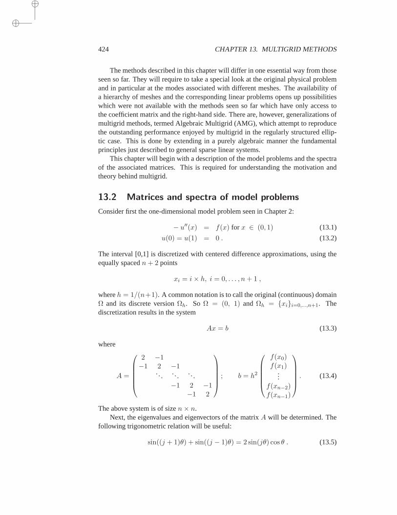
424 CHAPTER 13. MULTIGRID METHODS
The methods described in this chapter will differ in one essential way from thoseseen so far. They will require to take a special look at the original physical problemand in particular at the modes associated with different meshes. The availability ofa hierarchy of meshes and the corresponding linear problems opens up possibilitieswhich were not available with the methods seen so far which have only access tothe coefficient matrix and the right-hand side. There are, however, generalizations ofmultigrid methods, termed Algebraic Multigrid (AMG), which attempt to reproducethe outstanding performance enjoyed by multigrid in the regularly structured ellip-tic case. This is done by extending in a purely algebraic manner the fundamentalprinciples just described to general sparse linear systems.
This chapter will begin with a description of the model problems and the spectraof the associated matrices. This is required for understanding the motivationandtheory behind multigrid.
13.2 Matrices and spectra of model problems
Consider first the one-dimensional model problem seen in Chapter 2:
− u′′(x) = f(x) for x ∈ (0, 1) (13.1)
u(0) = u(1) = 0 . (13.2)
The interval [0,1] is discretized with centered difference approximations,using theequally spacedn+ 2 points
xi = i× h, i = 0, . . . , n+ 1 ,
whereh = 1/(n+1). A common notation is to call the original (continuous) domainΩ and its discrete versionΩh. So Ω = (0, 1) and Ωh = xii=0,...,n+1. Thediscretization results in the system
Ax = b (13.3)
where
A =
2 −1−1 2 −1
.. . . . . . . .−1 2 −1
−1 2
; b = h2
f(x0)f(x1)
...f(xn−2)f(xn−1)
. (13.4)
The above system is of sizen× n.Next, the eigenvalues and eigenvectors of the matrixA will be determined. The
following trigonometric relation will be useful:
sin((j + 1)θ) + sin((j − 1)θ) = 2 sin(jθ) cos θ . (13.5)
13.2. MATRICES AND SPECTRA OF MODEL PROBLEMS 425
Consider the vectoru whose components aresin θ, sin 2θ, · · · , sinnθ. Using therelation (13.5) we find that
(A− 2(1− cos θ)I)u = sin ((n+ 1)θ) en
whereen is then-th column of the identity. The right-hand side in the above relationis equal to zero for the following values ofθ:
θk =kπ
n+ 1, (13.6)
For any integer valuek. Therefore, the eigenvalues ofA are
λk = 2(1− cos θk) = 4 sin2 θk
2k = 1, . . . , n, (13.7)
and the associated eigenvectors are given by:
wk =
sin θk
sin(2θk)...
sin(nθk)
. (13.8)
Thei-th component ofwk can be rewritten in the form
sinikπ
n+ 1= sin(kπxi)
and represents the value of the functionsin(kπx) at the discretization pointxi. Thiscomponent of the eigenvector may therefore be written
wk(xi) = sin(kπxi) . (13.9)
Note that these eigenfunctions satisfy the boundary conditionswk(x0) = wk(xn+1) =0. These eigenfunctions are illustrated in Figure 13.1 for the casen = 7.
Now consider the 2-D Poisson equation
−(∂2u
∂x2+∂2u
∂y2
)
= f in Ω (13.10)
u = 0 onΓ (13.11)
whereΩ is the rectangle(0, l1) × (0, l2) andΓ its boundary. Both intervals can bediscretized uniformly by takingn + 2 points in thex direction andm + 2 points inthey directions:
xi = i× h1, i = 0, . . . , n+ 1 ; yj = j × h2, j = 0, . . . ,m+ 1
whereh1 =
l1n+ 1
; h2 =l2
m+ 1.
For simplicity we now assume thath1 = h2.
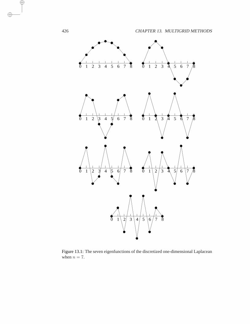
426 CHAPTER 13. MULTIGRID METHODS
0 1 2 3 4 5 6 7 8 0 1 2 3 4 5 6 7 8
0 1 2 3 4 5 6 7 8 0 1 2 3 4 5 6 7 8
0 1 2 3 4 5 6 7 8 0 1 2 3 4 5 6 7 8
0 1 2 3 4 5 6 7 8
Figure 13.1:The seven eigenfunctions of the discretized one-dimensional Laplaceanwhenn = 7.
13.2. MATRICES AND SPECTRA OF MODEL PROBLEMS 427
In this case the linear system has the form (13.3) whereA has the form
A =
B −I−I B −I
. .. .. . .. .−I B −I
−I B
with B =
4 −1−1 4 −1
. .. . .. . ..−1 4 −1
−1 4
.
The right-hand side is again the discrete version of the functionf scaled byh2.The above matrix can be represented in a succinct way using tensor product notation.Given anm× p matrixX and ann× q matrixY , the matrix
X ⊗ Y
can be viewed as a block matrix which has in (block) location(i, j) the matrixxijY .In other words,X⊗Y is of size(nm)×(pq) and is obtained by expanding each entryxij of X into the blockxijY . This definition is also valid for vectors by consideringthem as matrices (p = q = 1).
With this notation, the matrixA given above, can be written as
A = I ⊗ Tx + Ty ⊗ I, (13.12)
in which Tx abdTy are tridiagonal matrices of the same form as the matrixA in(13.4) and of dimensionn andm respectively. Often, the right-hand side of (13.12)is called thetensor sumof Tx andTy and is denoted byTx ⊕ Ty. A few simpleproperties are easy to show (see Exercise 1) for tensor products andtensor sums.One that is important for determining the spectrum ofA is
(Tx ⊕ Ty)(v ⊗ w) = v ⊗ (Txw) + (Tyv)⊗ w . (13.13)
In particular ifwk is an eigenvector ofTx associated withσk andvl is an eigenvectorof Tl associated withµl, it is clear that
(Tx ⊕ Ty)(vl ⊗ wk) = vl ⊗ (Txwk) + (Tyvk)⊗ wk = (σk + µl) vl ⊗ wk .
So,λkl = σk + µl is an eigenvalue ofA for each pair of eigenvaluesσk ∈ Λ(Tx)andµk ∈ Λ(Ty). The associated eigenvector isvl ⊗ wk. These eigenvalues andassociated eigenvectors are best labeled with two indices:
λkl = 2
(
1− coskπ
n+ 1
)
+ 2
(
1− coslπ
m+ 1
)
= 4
(
sin2 kπ
2(n+ 1)+ sin2 lπ
2(m+ 1)
)
. (13.14)
Their associated eigenvectorszk,l are
zk,l = vl ⊗ wk
428 CHAPTER 13. MULTIGRID METHODS
and they are best expressed by their values at the points(xi, yj) on the grid:
zk,l(xi, yj) = sin(kπxi) sin(lπyj) .
When all the sumsσk + µl are distinct this gives all the eigenvalues and eigenvec-tors ofA. Otherwise, we must show that the multiple eigenvalues correspond toindependent eigenvectors. In fact it can be shown that the system
vl ⊗ wkk=1,...,n; l=1...,m
is an orthonormal system if both the system of thevl’s and thewk’s are orthonormal.
13.2.1 Richardson’s iteration
Multigrid can be easily motivated by taking an in-depth look at simple iterativeschemes such as the Richardson iteration and Jacobi’s method. Note that these twomethods are essentially identical for the model problems under consideration, be-cause the diagonal of the matrix is a multiple of the identity matrix. Richardson’siteration is considered here for the one-dimensional case, using a fixed parameterω.In the next section, the weighted Jacobi iteration is fully analyzed with an emphasison studying the effect of varying the parameterω.
Richardson’s iteration takes the form:
uj+1 = uj + ω(b−Auj) = (I − ωA)uj + ωb .
Thus, the iteration matrix isMω = I − ωA . (13.15)
Recall from Example 4.1 from Chapter 4, that convergence takes place for 0 < ω <2/ρ(A). In realistic situations, the optimalω given by (4.33) is difficult to use.Instead, an upper boundρ(A) ≤ γ is often available from, e.g., Gershgorin’s the-orem, and we can simply takeω = 1/γ. This yields a converging iteration since1/γ ≤ 1/ρ(A) < 2/ρ(A).
By the relation (13.15), the eigenvalues of the iteration matrix are1−ωλk, whereλk is given by (13.7). The eigenvectors are the same as those ofA. If u∗ is the exactsolution, it was seen in Chapter 4 that the error vectordj ≡ u∗ − uj , obeys therelation,
dj = M jωd0 . (13.16)
It is useful to expand the error vectord0 in the eigenbasis ofMω, as
d0 =n∑
k=1
ξkwk .
From (13.16) and (13.15) this implies that at stepj,
dj =n∑
k=1
(
1− λk
γ
)j
ξkwk .
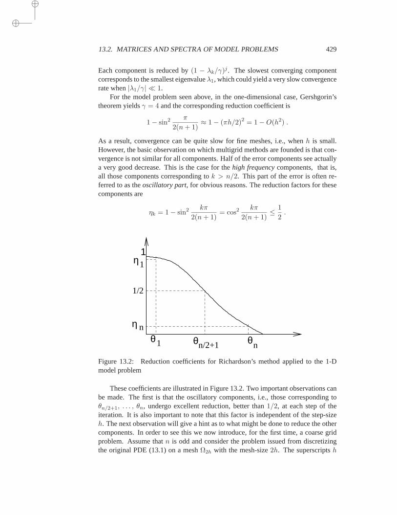
13.2. MATRICES AND SPECTRA OF MODEL PROBLEMS 429
Each component is reduced by(1 − λk/γ)j . The slowest converging component
corresponds to the smallest eigenvalueλ1, which could yield a very slow convergencerate when|λ1/γ| ≪ 1.
For the model problem seen above, in the one-dimensional case, Gershgorin’stheorem yieldsγ = 4 and the corresponding reduction coefficient is
1− sin2 π
2(n+ 1)≈ 1− (πh/2)2 = 1−O(h2) .
As a result, convergence can be quite slow for fine meshes, i.e., whenh is small.However, the basic observation on which multigrid methods are founded is that con-vergence is not similar for all components. Half of the error components see actuallya very good decrease. This is the case for thehigh frequencycomponents, that is,all those components corresponding tok > n/2. This part of the error is often re-ferred to as theoscillatory part, for obvious reasons. The reduction factors for thesecomponents are
ηk = 1− sin2 kπ
2(n+ 1)= cos2
kπ
2(n+ 1)≤ 1
2.
η
η
n
1
n
1/2
1
1 n/2+1 θθθ
Figure 13.2: Reduction coefficients for Richardson’s method applied to the1-Dmodel problem
These coefficients are illustrated in Figure 13.2. Two important observations canbe made. The first is that the oscillatory components, i.e., those corresponding toθn/2+1, . . . , θn, undergo excellent reduction, better than1/2, at each step of theiteration. It is also important to note that this factor is independent of the step-sizeh. The next observation will give a hint as to what might be done to reduce the othercomponents. In order to see this we now introduce, for the first time, a coarse gridproblem. Assume thatn is odd and consider the problem issued from discretizingthe original PDE (13.1) on a meshΩ2h with the mesh-size2h. The superscriptsh

430 CHAPTER 13. MULTIGRID METHODS
and2h will now be used to distinguish between quantities related to each grid. Thegrid points on the coarser mesh arex2h
i = i ∗ (2h). The second observation is basedon the simple fact thatx2h
i = xh2i from which it follows that, fork ≤ n/2,
whk(xh
2i) = sin(kπxh2i) = sin(kπx2h
i ) = w2hk (x2h
i ) .
In other words, taking a smooth mode on the fine grid (whk with k ≤ n/2) and
canonically injecting it into the coarse grid, i.e., defining its values on the coarsepoints to be the same as those on the fine points, yields thek-th mode on the coarsegrid. This is illustrated in Figure 13.3 fork = 2 and grids of9 points (n = 7) and5points (n = 3).
Some of the modes which were smooth on the fine grid, become oscillatory. Forexample, whenn is odd, the modewh
(n+1)/2 becomes precisely the highest mode onΩ2h. At the same time the oscillatory modes on the fine mesh are no longer rep-resented on the coarse mesh. The iteration fails to make progress on the finegridwhen the only components left are those associated with the smooth modes. Multi-grid strategies do not attempt to eliminate these components on the fine grid. Instead,they first move down to a coarser grid where smooth modes are translated intooscil-latory ones. Practically, this requires going back and forth between different grids.The necessarygrid-transfer operations will be discussed in detail later.
0 1 2 3 4 5 6 7 8
Fine mesh
0 1 2 3 4
Coarse mesh
Figure 13.3: The modew2 on a fine grid(n = 7) and a coarse grid(n = 3).
13.2. MATRICES AND SPECTRA OF MODEL PROBLEMS 431
13.2.2 Weighted Jacobi iteration
In this section a weighted Jacobi iteration is considered and analyzed for both 1-Dand 2-D model problems. The standard Jacobi iteration is of the form
uj+1 = D−1(E + F )uj +D−1f .
The weighted version of this iteration uses a parameterω and combines the aboveiterate with the currentuj :
uj+1 = ω(D−1(E + F )uj +D−1f
)+ (1− ω)uj
=[(1− ω)I + ωD−1(E + F )
]uj + ωD−1f (13.17)
≡ Jωuj + fω . (13.18)
Using the relationE + F = D −A it follows that
Jω = I − ωD−1A . (13.19)
In particular note that whenA is SPD, the weighted Jacobi iteration will convergewhen0 < ω < 2/ρ(D−1A). In the case of our 1-D model problem the diagonal isD = 2I, so the following expression forJω is obtained,
Jω = (1− ω)I +ω
2(2I −A) = I − ω
2A. (13.20)
For the 2-D case, a similar result can be obtained in which the denominator 2 isreplaced by 4. The eigenvalues of the iteration matrix follow immediately from theexpression (13.7),
µk(ω) = 1− ω(
1− coskπ
n+ 1
)
= 1− 2ω
(
sin2 kπ
2(n+ 1)
)
. (13.21)
In the 2-D case, these become,
µk,l(ω) = 1− ω(
sin2 kπ
2(n+ 1)+ sin2 lπ
2(m+ 1)
)
.
Consider the 1-D case first. The sine termssin2(kπ/2(n + 1)) lie in between1−s2 ands2, in whichs = sin(π/2(n+1)). Therefore, the eigenvalues are boundedas follows:
(1− 2ω) + 2ωs2 ≤ µk(ω) ≤ 1− 2ωs2 . (13.22)
The spectral radius ofJω is
ρ(Jω) = max|(1− 2ω) + 2ωs2|, |1− 2ωs2| .
Whenω is < 0 or > 1, it can be shown thatρ(Jω) > 1 for h small enough (SeeProblem 1). Whenω is between 0 and 1, then the spectral radius is simply1−2ωs2 ≈1− ωπ2h2/2.
432 CHAPTER 13. MULTIGRID METHODS
It is interesting to note that the bestω in the interval[0, 1] is ω = 1, so noacceleration of the original Jacobi iteration can be achieved. On the otherhand, ifthe weighted Jacobi iteration is regarded as a smoother, the situation is different. Forthose modes associated withk > n/2, the termsin2 θk is≥ 1/2 so
1− 2ω < (1− 2ω) + 2ωs2 ≤ µk(ω) ≤ 1− 1
2ω . (13.23)
For example whenω = 1/2, then all reduction coefficients for the oscillatory modeswill be in between 0 and 3/4, thus guaranteeing again a reduction ofh. Forω = 2/3the eigenvalues are between -1/3 and 1/3, leading to a smoothing factor of 1/3.Thisis the best that can achievedindependently ofh.
For 2-D problems, the situation is qualitatively the same. The bound (13.22)becomes,
(1− 2ω) + ω(s2x + s2y) ≤ µk,l(ω) ≤ 1− ω(s2x + s2y) (13.24)
in which sx is the same ass andsy = sin(π/(2(m + 1))). The conclusion for thespectral radius and rate of convergence of the iteration is similar, in thatρ(Jω) ≈1−O(h2) and the bestω is one. In addition, the high-frequency modes are dampedwith coefficients which satisfy:
1− 2ω < (1− 2ω) + ω(s2x + s2y) ≤ µk,l(ω) ≤ 1− 1
2ω . (13.25)
As before,ω = 1/2 yields a smoothing factor of 3/4, andω = 3/5 yields, a smooth-ing factor of4/5. Here the best that can be done, is to takeω = 4/5.
13.2.3 Gauss-Seidel iteration
In pratice, Gauss-Seidel and red-black Gauss-Seidel relaxation aremore commonsmoothers than Jacobi or Richardson’s iterations. Also, SOR (withω 6= 1) is rarelyused as it is known that overrelaxation adds no benefit in general. Gauss-Seidel andSOR schemes are somewhat more difficult to analyze.
Consider the iteration matrix
G = (D − E)−1F (13.26)
in the one-dimensional case. The eigenvalues and eigenvectors ofG satisfy the rela-tion
[F − λ(D − E)]u = 0
thej-th row of which is
ξj+1 − 2λξj + λξj−1 = 0, (13.27)
whereξj is thej-component of the vectoru. The boundary conditionsξ0 = ξn+1 =0, should be added to the above equations. Note that becauseξn+1 = 0, equation(13.27) is valid whenj = n (despite the fact that entry(n, n+1) of F is not defined).
13.2. MATRICES AND SPECTRA OF MODEL PROBLEMS 433
This is a difference equation, similar to Equation (2.21) encountered in Chapter 2and and it can be solved similarly by seeking a general solution in the formξj = rj .Substituting in (13.27),r must satisfy the quadratic equation
r2 − 2λr + λ = 0,
whose roots are
r1 = λ+√
λ2 − λ, r2 = λ−√
λ2 − λ .
This leads to the general solutionξj = αrj1 + βrj
2. The first boundary conditionξ0 = 0, implies thatβ = −α. The boundary conditionξn+1 = 0 yields the equationin λ
(
λ+√
λ2 − λ)n+1
−(
λ−√
λ2 − λ)n+1
= 0 →(
(λ+√λ2 − λ)2
λ
)n+1
= 1 ,
in which it is assumed thatλ 6= 0. With the change of variablesλ ≡ cos2 θ, thisbecomes(cos θ ± i sin θ)2(n+1) = 1, where the sign± is positive whencos θ andsin θ are of the same sign and negative otherwise. Hence,
± 2(n+ 1)θ = ±2k π → θ = θk ≡kπ
n+ 1, k = 1, . . . , n (13.28)
Therefore the eigenvalues are of the formλk = cos2 θk, whereθk was defined above,i.e.,
λk = cos2kπ
n+ 1.
In fact this result could have been obtained in a simpler way. According to Theorem4.16 seen in Chapter 4, whenω = 1, the eigenvalues of SOR iteration matrix are thesquares of those of the corresponding Jacobi iteration matrix with the sameω, whichaccording to (13.21) (left side) areµk = cos[kπ/(n+ 1)].
Some care must be exercised when computing the eigenvectors. Thej-th com-ponent of the eigenvector is given byξj = rj
1 − rj2. Proceeding as before, we have
rj1 =
(
cos2 θk +√
cos4 θk − cos2 θk
)j= (cos θk)
j (cos θk ± i sin θk)j ,
where the± sign was defined before. Similarly,rj2 = (cos θk)
j (cos θk ∓ i sin θk)j
where∓ is the opposite sign from±. Therefore,
ξj = (cos θk)j[
(cos θk ∓ i sin θk)j − (cos θk ± i sin θk)
j]
= 2i (cos θk)j [± sin(jθk)] .

434 CHAPTER 13. MULTIGRID METHODS
0 1 2 3 4 5 6 7 8 9 10 11 12
k=1
0 1 2 3 4 5 6 7 8 9 10 11 12
k=2
0 1 2 3 4 5 6 7 8 9 10 11 12
k=3
0 1 2 3 4 5 6 7 8 9 10 11 12
k=4
0 1 2 3 4 5 6 7 8 9 10 11 12
k=5
0 1 2 3 4 5 6 7 8 9 10 11 12
k=7
0 1 2 3 4 5 6 7 8 9 10 11 12
k=8
0 1 2 3 4 5 6 7 8 9 10 11 12
k=9
0 1 2 3 4 5 6 7 8 9 10 11 12
k=10
0 1 2 3 4 5 6 7 8 9 10 11 12
k=11
Figure 13.4:The eigenfunctions of 13-point one-dimensional mesh (n = 11). Thecasek = 6 is omitted.
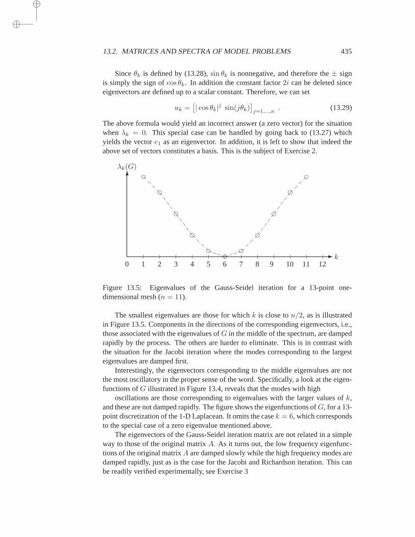
13.2. MATRICES AND SPECTRA OF MODEL PROBLEMS 435
Sinceθk is defined by (13.28),sin θk is nonnegative, and therefore the± signis simply the sign ofcos θk. In addition the constant factor2i can be deleted sinceeigenvectors are defined up to a scalar constant. Therefore, we can set
uk =[| cos θk|j sin(jθk)
]
j=1,...,n. (13.29)
The above formula would yield an incorrect answer (a zero vector) forthe situationwhenλk = 0. This special case can be handled by going back to (13.27) whichyields the vectore1 as an eigenvector. In addition, it is left to show that indeed theabove set of vectors constitutes a basis. This is the subject of Exercise 2.
0 1 2 3 4 5 6 7 8 9 10 11 12-
6
k
λk(G)
Figure 13.5: Eigenvalues of the Gauss-Seidel iteration for a 13-point one-dimensional mesh (n = 11).
The smallest eigenvalues are those for whichk is close ton/2, as is illustratedin Figure 13.5. Components in the directions of the corresponding eigenvectors, i.e.,those associated with the eigenvalues ofG in the middle of the spectrum, are dampedrapidly by the process. The others are harder to eliminate. This is in contrast withthe situation for the Jacobi iteration where the modes corresponding to the largesteigenvalues are damped first.
Interestingly, the eigenvectors corresponding to the middle eigenvalues are notthe most oscillatory in the proper sense of the word. Specifically, a look at the eigen-functions ofG illustrated in Figure 13.4, reveals that the modes with high
oscillations are those corresponding to eigenvalues with the larger values of k,and these are not damped rapidly. The figure shows the eigenfunctions of G, for a 13-point discretization of the 1-D Laplacean. It omits the casek = 6, which correspondsto the special case of a zero eigenvalue mentioned above.
The eigenvectors of the Gauss-Seidel iteration matrix are not related in a simpleway to those of the original matrixA. As it turns out, the low frequency eigenfunc-tions of the original matrixA are damped slowly while the high frequency modes aredamped rapidly, just as is the case for the Jacobi and Richardson iteration. This canbe readily verified experimentally, see Exercise 3
436 CHAPTER 13. MULTIGRID METHODS
13.3 Inter-grid operations
Multigrid algorithms require going back and forth between several grid problemsrelated to the solution of the same original equations. It is sufficient to present thesegrid transfer operations for the simple case of two meshes,Ωh (fine) andΩH (coarse),and to only consider the situation whenH = 2h. In particular, the problem size ofthe fine mesh problem will be about2d times as large as that of the coarse meshproblem, whered is the space dimension. In the previous section, the 1-D case wasalready considered and the subscripth corresponding to the mesh problem underconsideration was introduced.
13.3.1 Prolongation
A prolongation operation takes a vector fromΩH and defines the analogue vector inΩh. A common notation in use is:
IhH : ΩH −→ Ωh .
The simplest way to define a prolongation operator is through linear interpolation,which is now presented for the 1-D case first. The generic situation is that of n + 2points,x0, x1, . . . , xn+1 wherex0 andxn+1 are boundary points. The number ofinternal pointsn is assumed to be odd, so that halving the size of each subintervalamounts to introducing the middle points. Given a vector(v2h
i )i=0,...,(n+1)/2, thevectorvh = Ih
2hv2h of Ωh is defined as follows
vh2j = v2h
j
vh2j+1 = (v2h
j + v2hj+1)/2
for j = 0, . . . ,n+ 1
2.
In matrix form, the above defined prolongation can be written as
vh =1
2
121 1
21 1
...
...1 1
21
v2h . (13.30)
In 2-D, the linear interpolation can be defined in a straightforward manner fromthe 1-D case. Thinking in terms of a matrixvij representing the coordinate of afunction v at the pointsxi, yj , it is possible to define the interpolation in 2-D intwo stages. In the followingIh
x,2h denotes the interpolation in thex direction only
13.3. INTER-GRID OPERATIONS 437
andIhy,2h the interpolation fory variables only. First, interpolate all values in the
x-direction only:
vh,x = Ihx,2hv where
vh,x2i,: = v2h
i,:
vh,x2i+1,: = (v2h
i,: + v2hi+1,:)/2
for i = 0, . . . ,m+ 1
2.
Then interpolate this semi-interpolated result, with respect to they variable:
vh = Ihy,2hv
h,x where
vh:,2j = vx,2h
:,j
vh:,2j+1 = (vx,2h
:,j + vx,2h:,j+1)/2
for j = 0, . . . ,n+ 1
2.
This gives the following formulas for the 2-D interpolation of an elementvH in ΩH ,into the corresponding elementvh = Ih
H in Ωh,
vh2i,2j = v2h
ij
vh2i+1,2j = (v2h
ij + v2hi+1,j)/2
vh2i,2j+1 = (v2h
ij + v2hi,j+1)/2
vh2i+1,2j+1 = (v2h
ij + v2hi+1,j + v2h
i,j+1 + v2hi+1,j+1)/4
for
i = 0, . . . , n+1
2 ;
j = 0, . . . , m+12
.
From the above derivation, it is useful to observe that the 2-D interpolation can beexpressed as the tensor product of the two one-dimensional interpolations, i.e.,
Ih2h = Ih
y,2h ⊗ Ihx,2h. (13.31)
This is the subject of Exercise 4.It is common to represent the prolongation operators using a variation of the
stencil notation employed in Chapter 4 and Chapter 10. The stencil now operates ona grid to give values on a different grid. The one-dimensional stencil is denoted by
p =
]1
21
1
2
[
.
The open brackets notation only means that the stencil must be interpreted asa fan-out rather than fan-in operation as in the cases we have seen in earlier chapters. Inother words it is a column instead of a row operation, as can also be understood by alook at the matrix in (13.30). Each stencil is associated with a coarse grid point. Theresult of the stencil operation are the valuesvH
i /2, vHi , v
Hi /2, contributed to the three
fine mesh-pointsxh2i−1, x
h2i, andxh
2i+1 by the valuevHi . Another, possibly clearer,
interpretation is that the function with value one at the coarse grid pointx2hi , and zero
elsewhere, will be interpolated to a function in the fine mesh which has the values0.5, 1, 0.5 at the pointsxh
2i−1, xh2i, x
h2i+1, respectively, and zero elsewhere. Under
this interpretation, the stencil for the 2-D linear interpolation is
1
4
1 2 12 4 21 2 1
.
It is also interesting to note that the 2-D stencil can be viewed as a tensor product ofthe one dimensional stencilp and its transposepT . The stencilpT acts on the verticalcoordinates in exactly the same way thatp acts on the horizontal coordinates.
438 CHAPTER 13. MULTIGRID METHODS
Example 13.1. This example illustrates the use of the tensor product notation todetermine the 2-D stencil. The stencil can also be understood in terms of the actionof the interpolation operation on a unit vector. Using the stencil notation, this unitvector is of the formei ⊗ ej and we have (see Exercise 1)
Ih2h(ei ⊗ ej) = (Ih
y,2h ⊗ Ihx,2h)(ei ⊗ ej) = (Ih
y,2hei)⊗ (Ihx,2hej) .
When written in coordinate (or matrix) form this is a vector which corresponds tothe outer productppT with pT ≡ [12 1 1
2 ], centered at the point with coordinatexi, yj .
13.3.2 Restriction
The restriction operation is the reverse of prolongation. Given a functionvh on thefine mesh, a corresponding function inΩH must be defined fromvh. In the earlieranalysis one such operation was encountered. It was simply based on defining thefunctionv2h from the functionvh as follows
v2hi = vh
2i. (13.32)
Because this is simply a canonical injection fromΩh to Ω2h, it is termed theinjectionoperator. This injection has an obvious 2-D analogue:v2h
i,j = vh2i,2j .
A more common restriction operator, called full weighting (FW), definesv2h asfollows in the 1-D case:
v2hj =
1
4
(
vh2j−1 + 2vh
2j + vh2j+1
)
. (13.33)
This averages the neighboring values using the weights0.25, 0.5, 0.25. An importantproperty can be seen by considering the matrix associated with this definition of I2h
h :
I2hh =
1
4
1 2 11 2 1
1 2 1· · · · · · · · ·
1 2 1
. (13.34)
Apart from a scaling factor, this matrix is the transpose of the interpolation operatorseen earlier. Specifically,
Ih2h = 2 (I2h
h )T . (13.35)
The stencil for the above operator is
1
4[1 2 1]
where the closed brackets are now used to indicate the standard fan-in (row) opera-tion.
13.4. STANDARD MULTIGRID TECHNIQUES 439
In the 2-D case, the stencil for the full-weighting averaging is given by
1
16
1 2 12 4 21 2 1
.
This takes foruh2i,2j the result of a weighted average of the 9 pointsuH
i+q,j+p with|p|, |q| ≤ 1 with the associated weights2−|p|−|q|−2. Note that because the FullWeighting stencil is a scaled row (fan-in) version of the linear interpolation sten-cil, the matrix associated with the operatorI2h
h is essentially a transpose of theprolongation (interpolation) operator:
Ih2h = 4(I2h
h )T . (13.36)
The statements (13.35) and (13.36), can be summarized by
IhH = 2d(IH
h )T (13.37)
whered is the space dimension.The following relation can be shown
I2hh = I2h
y,h ⊗ I2hx,h (13.38)
which is analogous to (13.31) (see Exercise 5).
13.4 Standard multigrid techniques
One of the most natural ways to exploit a hierarchy of grids when solving PDEs, is toobtain an initial guess from interpolating a solution computed on a coarser grid. Theprocess can be recursively repeated until a given grid is reached. This interpolationfrom a coarser grid can be followed by a few steps of a smoothing iteration.Thisis known as nested iteration. General multigrid cycles are intrinsically recursiveprocesses which use essentially two main ingredients. The first is a hierarchy ofgrid problems along with restrictions and prolongations to move between grids.Thesecond is a smoother, i.e., any scheme which has the smoothing property of dampingquickly the high frequency components of the error. A few such schemes, such asthe Richardson and weighted Jacobi iterations, have been seen in earliersections.Other smoothers which are often used in practice are the Gauss-Seidel and Red-Black Gauss-Seidel iterations seen in Chapter 4.
13.4.1 Coarse problems and smoothers
At the highest level (finest grid) a mesh-size ofh is used and the resulting problemto solve is of the form:
Ahuh = fh .
One of the requirements of multigrid techniques is that a system similar to the oneabove must be solved at the coarser levels. It is natural to define this problem at the
440 CHAPTER 13. MULTIGRID METHODS
next level where a mesh of size, say,H, is used, as simply the system arising fromdiscretizing the same problem on the coarser meshΩH . In other cases, it may bemore useful to define the linear system byGalerkin projection, where the coarsegrid problem is defined by
AH = IHh AhI
hH , fH = IH
h fh . (13.39)
This formulation is more common in finite element methods. It also has some ad-vantages from a theoretical point of view.
Example 13.2. Consider the model problem in 1-D, and the situation whenAH
is defined from the Galerkin projection, i.e., via, formula (13.39), where thepro-longation and restriction operators are related by (13.35) (1-D) or (13.36) (2-D). In1-D,AH can be easily defined for the model problem when full-weighting is used.Indeed,
AHeHj = IH
h AhIhHe
Hj
= IHh Ah
[1
2eh2j−1 + eh2j +
1
2eh2j+1
]
= IHh
[
−1
2eh2j−2 + eh2j −
1
2eh2j+2
]
= −eHj−1 + 2eHj − eHj+1 .
This defines thej-th column ofAH , which has a 2 in the diagonal, -1 in the superand sub-diagonal and zero elsewhere. This means that the operatorAH defined bythe Galerkin property is identical with the operator that would be defined from acoarse discretization. This property is not true in 2-D when full weighting isused.see Exercise 6.
The notationuh
ν = smoothν(Ah, uh0 , fh)
means thatuhν is the result ofν smoothing steps for solving the above system, starting
with the initial guessuh0 . Smoothing iterations are of the form
uhj+1 = Shu
hj + gh (13.40)
whereSh is the iteration matrix associated with one smoothing step. As was seen inearlier chapters, the above iteration can always be rewritten in the ‘preconditioning’form:
uhj+1 = uh
j +Bh(fh −Ahuhj ) (13.41)
where
Sh ≡ I −BhAh, Bh ≡ (I − Sh)A−1h gh ≡ Bhf
h . (13.42)

13.4. STANDARD MULTIGRID TECHNIQUES 441
The errordhν and residualrh
ν resulting fromν smoothing steps satisfy
dhν = (Sh)νdh
0 = (I −BhAh)νdh0 ; rν
h = (I −AhBh)νrh0 .
It will be useful later to make use of the following observation. Whenfh = 0 thengh is also zero and as a result, one step of the iteration (13.40) will provide the resultof one product with the operatorSh.
Example 13.3. For example, settingf ≡ 0 in (13.17), yields the Jacobi iterationmatrix,
B = (I −D−1(E + F ))A−1 = D−1(D − E − F )A−1 = D−1 .
In a similar way one finds that for the Gauss-Seidel iteration,B = (D−E)−1F andfor Richardson iterationB = ωI.
Nested iteration was mentioned earlier as a means of obtaining good initialguesses from coarser meshes in a recursive way. The algorithm, presented here to il-lustrate the notation just introduced is described below. The assumption is thattherearep+ 1 grids, with mesh sizesh, 2h, . . . , 2pn ≡ h0.
ALGORITHM 13.1 Nested Iteration
1. Seth := h0. Given an initial guessuh0 , setuh = smoothνp(Ah, u
h0 , f
h)2. Forl = p− 1, . . . , 0 Do
3. uh/2 = Ih/2h uh
4. h := h/2;5. uh := smoothνl(Ah, u
h, fh)6. End
In practice, nested iteration is not much used in this form. However, it providesthe foundation for one of the most effective multigrid algorithms, namely the FullMulti-Grid (FMG) which will be described in a later section.
13.4.2 Two-grid cycles
When a smoother is applied to a linear system at a fine level, the residual
rh = fh −Auh
obtained at the end of the smoothing step will typically still be large. However, itwill have small components in the space associated with the high-frequency modes.If these components are removed by solving the above system (exactly) atthe lowerlevel, then a better approximation should result. Two-grid methods are rarelyprac-tical because the coarse-mesh problem may still be too large to be solved exactly.However, they are useful from a theoretical point of view. In the following algorithmH = 2h.
442 CHAPTER 13. MULTIGRID METHODS
ALGORITHM 13.2 Two-Grid cycle
1. Pre-smooth: uh := smoothν1(Ah, uh0 , f
h)2. Get residual: rh = fh −Ahu
h
3. Coarsen: rH = IHh r
h
4. Solve: AHδH = rH
5. Correct: uh := uh + IhHδ
H
6. Post-smooth:uh := smoothν2(Ah, uh, fh)
It is clear that the result of one iteration of the above algorithm corresponds tosome iteration process of the form
uhnew = Mhu
h0 + gMh
.
In order to determine the operatorMh we exploit the observation made above thattaking fh = 0 provides the productMhu
h0 . Whenfh = 0, then in line 1 of the
algorithm, uh becomesSν1h u
h0 . In line 3, we haverH = IH
h (fh − AhSν1h ) =
IHh (−AhS
ν1h ). Following this process, the vectoruh resulting from one cycle of
the algorithm becomes
uhnew = Sν2
h [Sν1h u
h0 + Ih
HA−1H IH
h (−AhSν1h u
h0)].
Therefore, the 2-grid iteration operator is given by
MhH = Sν2
h [I − IhHA
−1H IH
h Ah]Sν1h .
The matrix inside the brackets,
THh = I − Ih
HA−1H IH
h Ah , (13.43)
acts as another iteration by itself known as thecoarse grid correction,which can beviewed as a particular case of the two-grid operator with no smoothing, i.e., withν1 = ν2 = 0. Note that theB preconditioning matrix associated with this iterationis, according to (13.42),Bh = Ih
HA−1H IH
h .An important property of the coarse grid correction operator is discussed in the
following lemma. It is assumed thatAh is symmetric positive definite.
Lemma 13.1 When the coarse grid matrix is defined via (13.39), then the coarsegrid correction operator (13.43) is a projector which is orthogonal with respect totheAh-inner product. In addition, the range ofTH
h isAh-orthogonal to the range ofIHh .
Proof. It suffices to show thatI − THh = Ih
HA−1H IH
h Ah is a projector:
(IhHA
−1H IH
h Ah)×(IhHA
−1H IH
h Ah) = IhHA
−1H (IH
h AhIhH)
︸ ︷︷ ︸
AH
A−1H IH
h Ah = IhHA
−1H IH
h Ah.

13.4. STANDARD MULTIGRID TECHNIQUES 443
That IhHA
−1H IH
h Ah is an A-orthogonal projector follows from its self-adjointnesswith respect to theAh-inner product (see Chapter 1):
(THh x, y)Ah
= (AhIhHA
−1H IH
h Ahx, y) = (x,AhIhHA
−1H IH
h Ahy) = (x, THh y)Ah
.
Finally, the statement thatRan(THh ) is orthogonal toRan(IH
h ) is equivalent to stat-ing that for allx of the formx = TH
h y, we haveIHh Ahx = 0 which is readily
verified.
13.4.3 V-cycles and W-cycles
Anyone familiar with recursivity will immediately think of the following practicalversion of the 2-grid iteration: apply the 2-grid cycle recursively until a coarseenough level is reached and then solve exactly (typically using a direct solver). Thisgives the algorithm described below, called the V-cycle multigrid. In the algorithm,H stands for2h andh0 for the coarsest mesh-size.
ALGORITHM 13.3 uh = V-cycle(Ah, uh0 , f
h)
1. Pre-smooth: uh := smoothν1(Ah, uh0 , f
h)2. Get residual: rh = fh −Ahu
h
3. Coarsen: rH = IHh r
h
4. If (H == h0)5. Solve: AHδ
H = rH
6. Else7. Recursion: δH = V-cycle(AH , 0, r
H)8. EndIf9. Correct: uh := uh + Ih
HδH
10. Post-smooth:uh := smoothν2(Ah, uh, fh)
11. Returnuh
Consider the cost of one cycle, i.e., one iteration of the above algorithm. A fewsimple assumptions are needed along with new notation. The number of nonzeroelements ofAh is denoted bynnzh. It is assumed thatnnzh ≤ αnh, whereα doesnot depend onh. The cost of each smoothing step is equal tonnzh while the cost ofthe transfer operations (interpolation and restriction) is of the formβnh where againβ does not depend onh. The cost at the level where the grid size ish, is given by
C(nh) = (α(ν1 + ν2) + 2β)nh + C(n2h) .
Noting thatn2h = nh/2 in the one-dimensional case, This gives the recurrencerelation
C(n) = ηn+ C(n/2) (13.44)
in which η = (α(ν1 + ν2) + 2β). The solution of this recurrence relations yieldsC(n) ≤ 2ηn. For 2-dimensional problems,nh = 4n2h and in this case the costbecomes≤ 7/3ηn.
444 CHAPTER 13. MULTIGRID METHODS
We now introduce the general multigrid cycle which generalizes the V-cycle seenabove. Once more, the implementation of the multigrid cycle is of a recursive nature.
ALGORITHM 13.4 uh = MG (Ah, uh0 , f
h, ν1, ν2, γ)
1. Pre-smooth: uh := smoothν1(Ah, uh0 , f
h)2. Get residual: rh = fh −Ahu
h
3. Coarsen: rH = IHh r
h
4. If (H == h0)5. Solve: AHδ
H = rH
6. Else7. Recursion: δH = MGγ(AH , 0, r
H , ν1, ν2, γ)8. EndIf9. Correct: uh := uh + Ih
HδH
10. Post-smooth:uh := smoothν2(Ah, uh, fh)
11. Returnuh
Notice now that there is a new parameter,γ, which determines how many times MGis iterated in Line 7. Each of the MG iterations in Line 7 takes the form
δHnew = MG(AH , δ
H , rH , ν1, ν2, γ) (13.45)
and this is iteratedγ times. The initial guess for the iteration isδH = 0 the secondargument to the MG call in line 7 shows. The caseγ = 1 yields the V-cycle multigrid.The caseγ = 2 is known as theW-cycle multigrid. The resulting inter-grid up anddown moves can be complex as is illustrated by the diagrams in Figure 13.6. Thecaseγ = 3 is rarely used.
Now consider the cost of the general multigrid cycle. The only significant dif-ference with the V-cycle algorithm is that the recursive call to MG is iteratedγ timesinstead of only once for the V-cycle. Therefore, the cost formula (13.44) becomes
C(n) = ηn+ γC(n/2), (1-D case) C(n) = ηn+ γC(n/4), (2-D case).(13.46)
It can easily be shown that the cost of each loop is still linear whenγ < 2 in 1-D andγ < 4 in the 2-D case, see Exercise 12. In other cases, the cost per cycle increases toO(n log2 n).
Example 13.4. This example illustrates the convergence behavior of the V-cyclemultigrid for solving a model Poisson problem with Dirichlet boundary conditionsin two-dimensional space. The problem considered is of the form :
−∆u = 13 sin(2πx)× sin(3πy) (13.47)
and has the exact solutionu(x, y) = sin(2πx)× sin(3πy). The Poisson equation isset on a square grid and discretized usingnx = ny = 33 points, including the two

13.4. STANDARD MULTIGRID TECHNIQUES 445
lev=1,γ=1 lev=2,γ=1 lev=3,γ=1 lev=4,γ=1
lev=1,γ=2 lev=2,γ=2 lev=3,γ=2
lev=3,γ=3
Figure 13.6: Representations of Various V-cycles and W-cycles
boundary points in each direction. This leads to a linear system of dimensionN =312 = 961. The V-cycle multigrid was tested with three smoothers: (1) The weightedJacobi relaxation withω = 2/3; (2) Gauss-Seidel relaxation, and (3) the red-blackGauss-Seidel relaxation. Various values ofν1 andν2, the number of pre- and post-smoothing steps, respectively, were used. Table 13.1 shows the convergence factorsρ as estimated from the expression,
ρ = exp
(1
klog‖rk‖2‖r0‖2
)
,
for each of the smoothers. Herek is the total number of smoothing steps taken.The convergence was stopped as soon as the 2-norm of the residual was reduced bya factor oftol = 10−8. The overall winner is clearly the Red-Black Gauss Seidelsmoother. It is remarkable that even with a number of total smoothing stepsν1 + ν2
as small as two, a reduction factor of less than 0.1 is achieved with RB-GS. Also,it is worth pointing out that whenν1 + ν2 is constant, the red-black Gauss-Seidelsmoother tends to perform better whenν1 andν2 are more or less balanced (comparethe case(ν1, ν2) = (0, 2) versus(ν1, ν2) = (1, 1) for example). In the asymptoticregime (or very largek), the two ratios should be identical in theory.
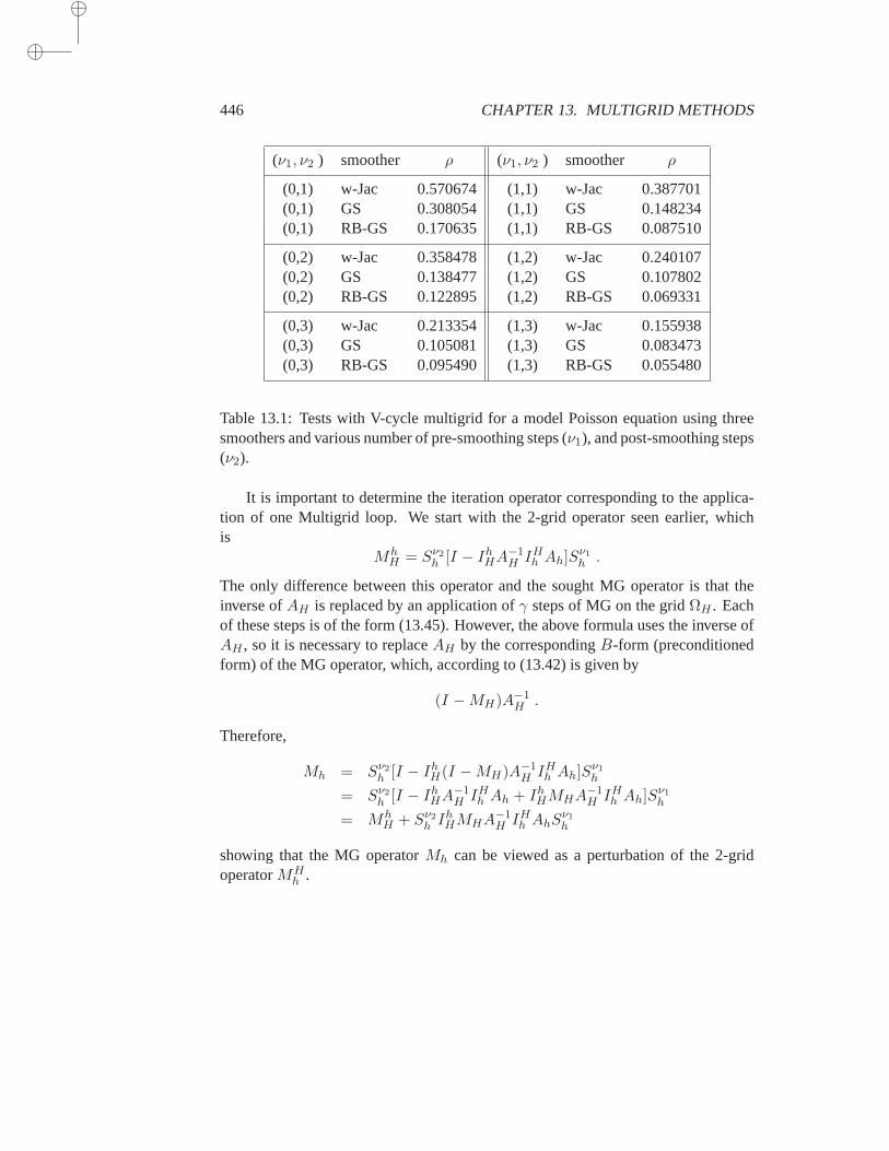
446 CHAPTER 13. MULTIGRID METHODS
(ν1, ν2 ) smoother ρ (ν1, ν2 ) smoother ρ
(0,1) w-Jac 0.570674 (1,1) w-Jac 0.387701(0,1) GS 0.308054 (1,1) GS 0.148234(0,1) RB-GS 0.170635 (1,1) RB-GS 0.087510
(0,2) w-Jac 0.358478 (1,2) w-Jac 0.240107(0,2) GS 0.138477 (1,2) GS 0.107802(0,2) RB-GS 0.122895 (1,2) RB-GS 0.069331
(0,3) w-Jac 0.213354 (1,3) w-Jac 0.155938(0,3) GS 0.105081 (1,3) GS 0.083473(0,3) RB-GS 0.095490 (1,3) RB-GS 0.055480
Table 13.1: Tests with V-cycle multigrid for a model Poisson equation using threesmoothers and various number of pre-smoothing steps (ν1), and post-smoothing steps(ν2).
It is important to determine the iteration operator corresponding to the applica-tion of one Multigrid loop. We start with the 2-grid operator seen earlier, whichis
MhH = Sν2
h [I − IhHA
−1H IH
h Ah]Sν1h .
The only difference between this operator and the sought MG operator isthat theinverse ofAH is replaced by an application ofγ steps of MG on the gridΩH . Eachof these steps is of the form (13.45). However, the above formula uses the inverse ofAH , so it is necessary to replaceAH by the correspondingB-form (preconditionedform) of the MG operator, which, according to (13.42) is given by
(I −MH)A−1H .
Therefore,
Mh = Sν2h [I − Ih
H(I −MH)A−1H IH
h Ah]Sν1h
= Sν2h [I − Ih
HA−1H IH
h Ah + IhHMHA
−1H IH
h Ah]Sν1h
= MhH + Sν2
h IhHMHA
−1H IH
h AhSν1h
showing that the MG operatorMh can be viewed as a perturbation of the 2-gridoperatorMH
h .
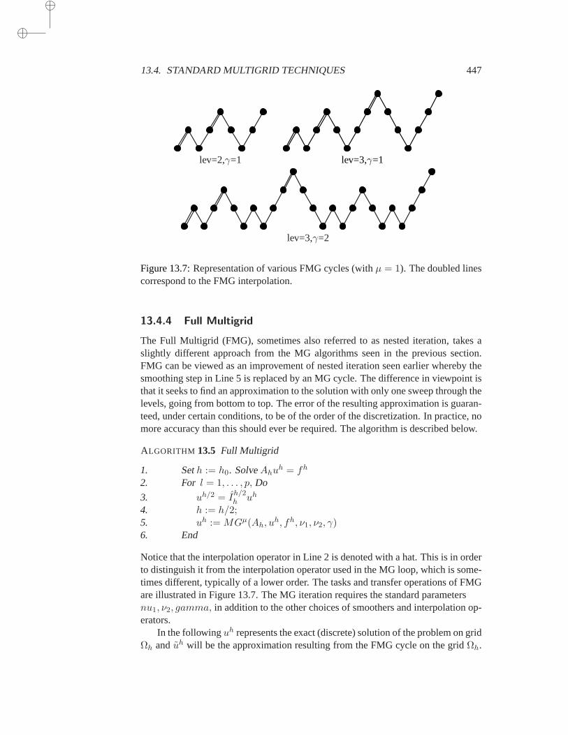
13.4. STANDARD MULTIGRID TECHNIQUES 447
lev=2,γ=1 lev=3,γ=1
lev=3,γ=2
Figure 13.7:Representation of various FMG cycles (withµ = 1). The doubled linescorrespond to the FMG interpolation.
13.4.4 Full Multigrid
The Full Multigrid (FMG), sometimes also referred to as nested iteration, takesaslightly different approach from the MG algorithms seen in the previous section.FMG can be viewed as an improvement of nested iteration seen earlier whereby thesmoothing step in Line 5 is replaced by an MG cycle. The difference in viewpoint isthat it seeks to find an approximation to the solution with only one sweep throughthelevels, going from bottom to top. The error of the resulting approximation is guaran-teed, under certain conditions, to be of the order of the discretization. In practice, nomore accuracy than this should ever be required. The algorithm is described below.
ALGORITHM 13.5 Full Multigrid
1. Seth := h0. SolveAhuh = fh
2. For l = 1, . . . , p, Do
3. uh/2 = Ih/2h uh
4. h := h/2;5. uh := MGµ(Ah, u
h, fh, ν1, ν2, γ)6. End
Notice that the interpolation operator in Line 2 is denoted with a hat. This is in orderto distinguish it from the interpolation operator used in the MG loop, which is some-times different, typically of a lower order. The tasks and transfer operations of FMGare illustrated in Figure 13.7. The MG iteration requires the standard parametersnu1, ν2, gamma, in addition to the other choices of smoothers and interpolation op-erators.
In the followinguh represents the exact (discrete) solution of the problem on gridΩh anduh will be the approximation resulting from the FMG cycle on the gridΩh.
448 CHAPTER 13. MULTIGRID METHODS
Thus,uh is the result of Line 5 in Algorithm 13.5. One of the main assumptions madein analyzing FMG is that the exact solution of the discrete linear systemAhu
h = fh
is close, within the discretization accuracy, to the exact solution of the PDE problem:
‖u− uh‖ ≤ chκ. (13.48)
The left-hand side represents the norm of the difference between the exact solutionuh of the discrete problem and the solution of the continuous problem sampled atthegrid points ofΩh. Any norm onΩh can be used, and the choice of the norm willreexamined shortly. Using an argument based on the triangle inequality, a particularconsequence of the above assumption is thatuh andIh
HuH should also be close since
they are close to the same (continuous) functionu. Specifically, the assumption(13.48) is replaced by:
‖uh − IhHu
H‖ ≤ c1hκ . (13.49)
A bound of this type can be shown by making a more direct assumption on theinterpolation operator, see Exercise 13. The next important assumption to make isthat the MG iteration operator is uniformly bounded,
‖Mh‖ ≤ ξ<1 . (13.50)
Finally, the interpolationIhH must also be bounded, a condition which is convenient
to state as follows,‖Ih
H‖ ≤ c22−κ . (13.51)
Theorem 13.2 Assume that (13.49), (13.50), and (13.51) are satisfied, and thatµ issufficiently large that
c2ξµ < 1 . (13.52)
Then the FMG iteration produces approximationsuh, which at each level satisfy,
‖uh − uh‖ ≤ c3c1hκ (13.53)
withc3 = ξµ/(1− c2ξµ) . (13.54)
Proof. The proof is by induction. At the lowest level, equation (13.53) is clearlysatisfied because the solutionuh is exact at the coarsest level and so the error iszero. Consider now the problem associated with the mesh sizeh and assume that thetheorem is valid for the mesh sizeH. The error vector is given by
uh − uh = (Mh)µ(uh − uh0). (13.55)
The initial guess is defined byuh0 = Ih
H uH . Therefore,
‖uh − uh0‖ = ‖uh − Ih
HuH + Ih
H(uH − uH)‖≤ ‖uh − Ih
HuH‖+ ‖Ih
H(uH − uH)‖≤ c1h
κ + ‖IhH‖c1c3Hκ (by (13.49) and induction hypothesis
≤ hκ(c1 + 2−κc2Hκc1c3) (by (13.51))
≤ hκc1(1 + c2c3) .
13.4. STANDARD MULTIGRID TECHNIQUES 449
Combining the above with (13.55) and (13.50) yields
‖uh − uh‖ ≤ ξµhκc1(1 + c2c3) .
From the relation (13.54), we getξµ = c3/(1+c2c3) and this shows the result (13.53)for the next level and completes the induction proof.
In practice it is accepted that takingµ = 1 is generally sufficient to satisfy the as-sumptions of the theorem. For example, if‖Ih
H‖ ≤ 1, andκ = 1, thenc2 = 4. In thiscase, withµ = 1, the result of the theorem will be valid providedξ < 0.25, which iseasily achieved by a simple V-cycle using Gauss-Seidel smoothers.
Example 13.5. This example illustrates the behavior of the full multigrid cyclewhen solving the same model Poisson problem as in Example 13.4. As before,thePoisson equation is set on a square grid and discretized with centered differences.The problem is solved using the mesh sizesnx = ny = 9, 17, 33, 65, and129 points(including the two boundary points) in each direction. Thus, for example, the lastproblem leads to a linear system of dimensionN = 1272 = 16, 129.
Figure 13.8 shows in log scale the 2-norm of the actual error achieved for threeFMG schemes as a function oflog(nx − 1). It also shows the 2-norm of the dis-cretization error. Note that whennx = 9, all methods show the same error as thediscretization error because the system is solved exactly at the coarsestlevel, i.e.,whennx = 9. The first FMG scheme uses a weighted Jacobi iteration with theweightω = 2/3, and(ν1, ν2) = (1, 0). As can be seen the error achieved becomestoo large relative to the discretization error when the number of levels increases. Onthe other hand, the other two schemes, RB-GS with(ν1, ν2) = (4, 0) and GS with(ν1, ν2) = (2, 0) perform well. It is remarkable that the error achieved by RB-GS isactually slightly smaller than the discretization error itself.
The result of the above theorem is valid in any norm. However, it is importanttonote that the type of bound obtained will depend on the norm used.
Example 13.6. It is useful to illustrate the basic discretization error bound (13.48)for the 1-D model problem. As before, we abuse the notation slightly by denoting byu the vector inΩh whose values at the grid points are the values of the (continuous)solutionu of the differential equation (13.1–13.2). Now the discreteL2-norm onΩh, denoted by‖v‖h will be used. In this particular case, this norm is also equal toh1/2‖v‖2, the Euclidean norm scaled by
√h. Then we note that,
‖uh − u‖h = ‖(Ah)−1Ah(uh − u)‖h = ‖(Ah)−1[fh −Ahu]‖h≤ ‖(Ah)−1‖h ‖fh −Ahu‖h . (13.56)
Assuming that the continuousu is inC4, (four times differentiable with continuousfourth derivative), Equation (2.12) from Chapter 2 gives
(f −Ahu)i = fi + u′′(xi) +h2
12u(4)(ξi) =
h2
12u(4)(ξi)
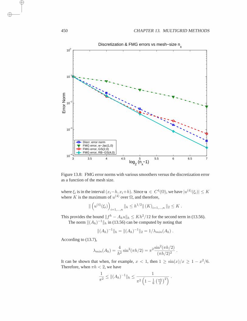
450 CHAPTER 13. MULTIGRID METHODS
3 3.5 4 4.5 5 5.5 6 6.5 710
−4
10−3
10−2
10−1
100
Discretization & FMG errors vs mesh−size nx
log2 (n
x −1)
Err
or N
orm
Discr. error norm FMG error, w−Jac(1,0)FMG error, GS(2,0) FMG error, RB−GS(4,0)
Figure 13.8: FMG error norms with various smoothers versus the discretization erroras a function of the mesh size.
whereξi is in the interval(xi−h, xi+h). Sinceu ∈ C4(Ω), we have|u(4)(ξi)| ≤ KwhereK is the maximum ofu(4) overΩ, and therefore,
‖(
u(4)(ξi))
i=1,...,n‖h ≤ h1/2‖ (K)i=1,...,n ‖2 ≤ K .
This provides the bound‖fh −Ahu‖h ≤ Kh2/12 for the second term in (13.56).The norm‖(Ah)−1‖h in (13.56) can be computed by noting that
‖(Ah)−1‖h = ‖(Ah)−1‖2 = 1/λmin(Ah) .
According to (13.7),
λmin(Ah) =4
h2sin2(πh/2) = π2 sin2(πh/2)
(πh/2)2.
It can be shown that when, for example,x < 1, then1 ≥ sin(x)/x ≥ 1 − x2/6.Therefore, whenπh < 2, we have
1
π2≤ ‖(Ah)−1‖h ≤
1
π2(
1− 16
(πh2
)2) .
13.5. ANALYSIS FOR THE TWO-GRID CYCLE 451
Putting these results together yields the inequality:
‖uh − u‖h ≤K
12π2(
1− 16
(πh2
)2) h2 .
Exercise 16 considers an extension of this argument to 2-D problems. Exercise 17explores what happens if other norms are used.
13.5 Analysis for the two-grid cycle
The two-grid correction cycle is at the basis of most of the more complex multigridcycles. For example, it was seen that the general MG cycle can be viewedas aperturbation of a 2-Grid correction cycle. Similarly, practical FMG schemesuse aV-cycle iteration for their inner loop. This section will take a in-depth look at theconvergence of the 2-grid cycle, for the case when the coarse grid problem is definedby the Galerkin approximation (13.39). This case is important in particular becauseit is at the basis of all the algebraic multigrid techniques which will be covered inthenext section.
13.5.1 Two important subspaces
Consider the two-grid correction operatorTHh defined by (13.43). As was seen in
Section 13.4.2, see Lemma 13.1, this is anAh-orthogonal projector onto the subspaceΩh. It is of the formI −Qh where
Qh = IhHA
−1H IH
h Ah .
Clearly,Qh is also anAh-orthogonal projector (sinceI −Qh is, see Chapter 1), andwe have
Ωh = Ran(Qh)⊕Null(Qh) ≡ Ran(Qh)⊕ Ran(I −Qh) . (13.57)
The definition ofQh implies that
Ran(Qh) ⊂ Ran(IhH) .
As it turns out, the inclusion also holds in the other direction, which means that thetwo subspaces are the same. To show this, take a vectorz in the range ofIh
H , soz = Ih
Hy for a certainy ∈ Ωh. Remembering thatAH = IHh AhI
hH , we obtain
Qhz = IhHA
−1H IH
h Ah IhHy = Ih
Hy = z ,
which shows thatz belongs toRan(Qh). Hence,
Ran(Qh) = Ran(IhH) .
452 CHAPTER 13. MULTIGRID METHODS
This says thatQh is theAh- orthogonal projector onto the spaceRan(IhH), while
THh is theAh- orthogonal projector onto the orthogonal complement. This orthog-
onal complement, which is the range ofI − Qh, is also the null space ofQh ac-cording to the fundamental relation (1.58) of Chapter 1. Finally, the null space ofQh is identical with the null space of the restriction operatorIH
h . It is clear thatNull(IH
h ) ⊂ Null(Qh). The reverse inclusion is not as clear and may be derivedfrom the fundamental relation (1.18) seen in Chapter 1. This relation implies that
Ωh = Ran(IhH)⊕Null
(
(IhH)T
)
= Ran(Qh)⊕Null(
(IhH)T
)
.
However, by (13.37),Null((Ih
H)T)
= Null(IHh ). Comparing this with the decom-
position (13.57), it follows that
Null(Qh) = Null(IHh ) .
In summary, if we set
Sh ≡ Ran(Qh) , Th ≡ Ran(THh ) (13.58)
then the following relations can be stated:
Ωh = Sh ⊕ Th (13.59)
Sh = Ran(Qh) = Null(Th) = Ran(IhH) (13.60)
Th = Null(Qh) = Ran(Th) = Null(IHh ) . (13.61)
These two subspaces are fundamental when analyzing MG methods. Intuitively,it can be guessed that the null space ofTH
h is somewhat close to the space of smoothmodes. This is because it is constructed so that its desired action on a smooth com-ponent is to annihilate it. On the other hand it should leave an oscillatory componentmore or less unchanged. Ifs is a smooth mode andt an oscillatory one, then thistranslates into the rough statements,
THh s ≈ 0, TH
h t ≈ t .
Clearly, opposite relations are true withQh, namelyQht ≈ 0 andQhs ≈ s.
Example 13.7. Consider the case when the prolongation operatorIHh corresponds
to the case of full weighting in the one-dimensional case. Consider the effect of thisoperator on any eigenmodewh
k , which has componentssin(jθk) for j = 1, . . . , n.whereθk = kπ/(n+ 1). Then, according to (13.33)
(IHh w
hk)j =
1
4[sin((2j − 1)θk) + 2 sin(2jθk) + sin((2j + 1)θk)]
=1
4[2 sin(2jθk) cos θk + 2 sin(2jθk)]
=1
2(1 + cos θk) sin(2jθk)
= cos2(θk
2
)
sin(2jθk) .
13.5. ANALYSIS FOR THE TWO-GRID CYCLE 453
Consider a modewk wherek is large, i.e., close ton. Then,θk ≈ π. In this case, therestriction operator will transform this mode into a constant times the same mode onthe coarser grid. The multiplicative constant, which iscos2(θk/2), is close to zeroin this situation, indicating thatIH
h wk ≈ 0, i.e., thatwk is near the null space ofIHh . Oscillatory modes are close to being in the null space ofIH
h , or equivalently therange ofTH
h .Whenk is small, i.e., for smooth modes, the constantcos2(θk/2) is close to
one. In this situation the interpolation produces the equivalent smooth mode inΩH
without damping it.
13.5.2 Convergence analysis
When analyzing convergence for the Galerkin case, theAh norm is often used. Inaddition, 2-norms weighted byD1/2, orD−1/2, whereD is the diagonal ofA, areconvenient. For example, we will use the notation,
‖x‖D = (Dx, x)1/2 ≡ ‖D1/2x‖2 .
The following norm also plays a significant role,
‖e‖AhD−1Ah= (D−1Ahe,Ahe)
1/2 ≡ ‖Ahe‖D−1 .
To avoid burdening the notation unnecessarily we simply use‖Ahe‖D−1 to denotethis particular norm ofe. It can be shown that standard 2-grid cycles satisfy aninequality of the form,
‖Sheh‖2Ah
≤ ‖eh‖2Ah− α‖Aeh‖2D−1 ∀ eh ∈ Ωh (13.62)
independently ofh. This is referred to as thesmoothing property.In addition to the above requirement which characterizes the smoother, another
assumption will be made which characterizes the discretization. This assumptionisreferred to as theapproximation property, and can be stated as follows:
minuH∈ΩH
‖eh − IhHe
H‖2D ≤ β‖eh‖2Ah, (13.63)
whereβ does not depent onh. In the following theorem, it is assumed thatA is SPD,and that the restriction and prolongation operators are linked by a relation of the form(13.37), withIh
H being of full rank.
Theorem 13.3 Assume that inequalities (13.62) and (13.63) are satisfied for a cer-tain smoother, whereα > 0 and β > 0. Thenα ≤ β, the two-level iterationconverges, and the norm of its operator is bounded as follows:
‖ShTHh ‖Ah
≤√
1− α
β. (13.64)
454 CHAPTER 13. MULTIGRID METHODS
Proof. It was seen in the previous section thatRan(THh ) = Th is Ah-orthogonal to
Ran(IhH) = Sh. As a result,(eh, Ih
HeH)Ah
= 0 for anyeh ∈ Ran(THh ), and so,
‖eh‖2Ah= (Ahe
h, eh − IhHe
H) ∀ eh ∈ Ran(THh ).
For anyeh ∈ Ran(THh ), the cauchy-schwarz inequality gives
‖eh‖2Ah= (D−1/2Ahe
h, D1/2(eh − IhHe
H))
≤ ‖D−1/2Aheh‖2 ‖D1/2(eh − Ih
HeH)‖2
= ‖Aheh‖D−1 ‖eh − Ih
HeH‖D .
By (13.63), this implies that‖eh‖Ah≤ √β‖Ahe
h‖D−1 for anyeh ∈ Ran(T hH), or
equivalently,‖THh eh‖2Ah
≤ β‖AhThHe
h‖2D−1 for any eh in Ωh. The proof is com-pleted by exploiting the smoothing property, i.e., inequality (13.62),
0 ≤ ‖ShTHh eh‖2Ah
≤ ‖THh eh‖2Ah
− α‖AhTHh eh‖2D−1
≤ ‖THh eh‖2Ah
− α
β‖TH
h eh‖2Ah
=
(
1− α
β
)
‖THh eh‖2Ah
≤(
1− α
β
)
‖eh‖2Ah.
The fact thatTHh is anAh-orthogonal projector was used to show the last step.
Example 13.8. As an example, we will explore the smoothing property (13.62) inthe case of the weighted Jacobi iteration. The indexh is now dropped for clarity.From (13.19) the smoothing operator in this case is
S(ω) ≡ I − ωD−1A .
WhenA is SPD, then the weighted Jacobi iteration will converge for0 < ω <2/ρ(D−1A). For any vectore we have
‖S(ω)e‖2A = (A(I − ωD−1A)e, (I − ωD−1Ae))
= (Ae, e)− 2ω(AD−1Ae, e) + ω2(AD−1Ae,D−1Ae)
= (Ae, e)− 2ω(D− 12Ae,D− 1
2Ae) + ω2(
(D− 12AD− 1
2 )D− 12Ae,D− 1
2Ae)
= (Ae, e)−([
ω(2I − ωD− 12AD− 1
2 )]
D− 12Ae,D− 1
2Ae)
≤ ‖e‖2A − λmin
[
ω(2I − ωD− 12AD− 1
2 )]
‖Ae‖2D−1 . (13.65)
Let γ = ρ(D− 12AD− 1
2 ) = ρ(D−1A). Then the above restriction onω impliesthat2 − ωγ > 0, and the matrix in the brackets in (13.65) is positive definite withminimum eigenvalueω(2− ωγ). Then, it suffices to take
α = ω(2− ωγ)
13.6. ALGEBRAIC MULTIGRID 455
to satisfy the requirement (13.62). Note that (13.62) is also valid withα replacedby any positive number that does not exceed the above value, but inequality whichwould result would be less sharp. Exercise 15 explores the same questionwhenRichardson’s iteration is used instead of weighted Jacobi.
13.6 Algebraic Multigrid
Throughout the previous sections of this chapter, it was seen that multigridmethodsdepend in a fundamental way on the availability of an underlying mesh. In addi-tion to this, the performance of multigrid deteriorates for problems with anisotropiccoefficients or discontinuous coefficients. It is also difficult to define multigrid ondomains that are not rectangular, especially in three dimensions. Given the successof these techniques, it is clear that it is important to consider alternatives which usesimilar principles which do not face the same disadvantages. Algebraic multigridmethods have been defined to fill this gap. The main strategy used in AMG is toexploit the Galerkin approach, see Equation (13.39), in which the interpolation andprolongation operators are defined in an algebraic way, i.e., only from theknowledgeof the matrix.
In this section the matrixA is assumed to be positive definite. Since meshesare no longer available, the notation must be changed, or interpreted differently, toreflect levels rather than grid sizes. Hereh is no longer a mesh-size but an index toa certain level, andH is used to index a coarser level. The meshΩh is now replacedby a subspaceXh ofRn at a certain level andXH denotes the subspace of the coarseproblem. Since there are no meshes, one might wonder how the coarse problems canbe defined.
In AMG, the coarse problem is typically defined using the Galerkin approach,which we restate here:
AH = IHh AhI
hH , fH = IH
h fh (13.66)
whereIHh the restriction operator, andIh
H the prolongation operator, both definedalgebraically. The prolongation and restriction operators are now relatedby transpo-sition:
IHh = (Ih
H)T . (13.67)
A minimum assumption made on the prolongation operator is that it is of full rank.It can therefore be said that only two ingredients are required to generalize the
multigrid framework:
1. A way to define the ‘coarse’ subspaceXH from a fine subspaceXh;
2. A way to define the interpolation operatorIHh fromXh toXH .
In other words, all that is required is a scheme forcoarseninga fine space along withan interpolation operator which would map a coarse node into a fine one.
456 CHAPTER 13. MULTIGRID METHODS
In order to understand the motivations for the choices made in AMG when defin-ing the above two components, it is necessary to extend the notion of smooth andoscillatory modes. This is examined in the next section.
Note that Lemma 13.1 is valid and it implies thatTHh is a projector, which is
orthogonal when theAh inner product is used. The corresponding relations (13.59– 13.61) also hold. Therefore, Theorem 13.3 is also valid and this is a fundamentaltool used in the analysis of AMG.
13.6.1 Smoothness in AMG
By analogy with multigrid, an error is decomposed into smooth and oscillatory com-ponents. However, these concepts are now defined with respect to the ability or in-ability of the smoother to reduce these modes. Specifically, an error is smooth whenits convergence with respect to the smoother is slow. The common way to state thisis to say that, for a smooth errors,
‖Shs‖A ≈ ‖s‖A .
Note the use of the energy norm which simplifies the analysis. If the smoother sat-isfies the smoothing property (13.62), then this means that for a smooth errors, wewould have
‖As‖D−1 ≪ ‖s‖Ah.
Expanding the norms and using the Cauchy-Schwarz inequality gives
‖s‖2Ah= (D−1/2Ahs,D
1/2s)
≤ ‖D−1/2Ahs‖2 ‖D1/2s‖2= ‖Ahs‖D−1 ‖s‖D .
Since‖As‖D−1 ≪ ‖s‖Ahthis means that‖s‖Ah
≪ ‖s‖D, or
(As, s)≪ (Ds, s) . (13.68)
It simplifies the analysis to setv = D1/2s. Then,
(D− 12AD− 1
2 v, v)≪ (v, v) .
The matrixA ≡ D− 12AD− 1
2 is a scaled version ofA in which the diagonal entriesare transformed into ones. The above requirement states that the Rayleighquotientof D1/2s is small. This is in good agreement with standard multigrid since, a smallRayleigh quotient implies that the vectorv is a linear combination of the eigenvectorsof A with smallest eigenvalues. In particular,(As, s) ≈ 0 also implies thatAs ≈ 0,i.e.,
aiisi ≈ −∑
j 6=i
aijsj . (13.69)
13.6. ALGEBRAIC MULTIGRID 457
It is also interesting to see how to interpret smoothness in terms of the matrix coeffi-cients. A common argument held in AMG methods exploits the following expansionof (As, s):
(As, s) =∑
i,j
aijsisj
=1
2
∑
i,j
−aij
((sj − si)
2 − s2i − s2j)
=1
2
∑
i,j
−aij(sj − si)2 +
∑
i
∑
j
aij
s2i .
The condition (13.68) can be rewritten as(As, s) = ǫ(Ds, s), in which0 < ǫ ≪ 1.For the special case when the row-sums of the matrix are zero, and the off-diagonalelements are negative, then this gives,
1
2
∑
i,j
|aij |(sj−si)2 = ǫ
∑
i
aiis2i →
∑
i
aiis2i
∑
j 6=i
|aij |aii
(si − sj
si
)2
− 2ǫ
= 0 .
A weighted sum, with nonnegative weights, of the bracketed terms must vanish. Itcannot be rigorously argued that the bracketed term must be of the order 2ǫ, but onecan say thaton averagethis will be true, i.e.,
∑
j 6=i
|aij |aii
(si − sj
si
)2
≪ 1 . (13.70)
For the above relation to hold,|si− sj |/|si|must be small when|aji/aii| is large. Inother words, the components ofs vary slowly in the direction of the strong connec-tions. This observation is used in AMG when defining interpolation operatorsandfor coarsening.
13.6.2 Interpolation in AMG
The argument given at the end of the previous section is at the basis of many AMGtechniques. Consider a coarse nodei and its adjacent nodesj, i.e., those indicessuch thataij 6= 0. The argument following (13.70) makes it possible to distinguishbetween weak couplings,|aij/aii| is smaller than a certain thresholdσ, and strongcouplings, when it is larger. Therefore, there are three types of nodes among thenearest neighbors of a fine nodei. First there is a set of coarse nodes, denoted byCi.Then among the fine nodes we have a setF s
i of nodes that are strongly connectedwith i, and a setFw
i of nodes that are weakly connected withi. An illustration isshown in Figure 13.9. The smaller filled circles represent the fine nodes, and the thindashed lines represent the weak connections. The thick dash-dot linesrepresent thestrong connections.

458 CHAPTER 13. MULTIGRID METHODS
According to the argument given above, a good criterion for finding an interpola-tion formula is to use the relation (13.69) which heuristically characterizes a smootherror. This is because interpolation should average out, i.e., eliminate, highlyoscil-latory elements inXh, and produce a function that is smooth in the coarser space.Then we rewrite (13.69) as
aiisi ≈ −∑
j ∈ Ci
aijsj −∑
j ∈ F si
aijsj −∑
j ∈ F wi
aijsj . (13.71)
Consider eliminating the weak connections first. Instead of just removing themfromthe picture, it is natural to lump their action and add the result into the diagonal term,in a manner similar to the compensation strategy used in ILU. This gives,
aii +∑
j ∈ F wi
aij
si ≈ −∑
j ∈ Ci
aijsj −∑
j ∈ F si
aijsj . (13.72)
F
C
C
F
F
F
C
C
Figure 13.9: Example of nodes adjacent to a fine nodei (center). Fine mesh nodesare labeled with F, coarse nodes with C.
The end result should be a formula in which the right-hand side depends only oncoarse points. Therefore, there remains to express each of the terms ofthe secondsum in the right-hand side of the above equation, in terms of values at coarse points.Consider the termsj for j ∈ F s
i . At nodej, the following expression can be writtenthat is similar to (13.69)
ajjsj ≈ −∑
l ∈ Cj
ajlsl −∑
l ∈ F sj
ajlsl −∑
l ∈ F wj
ajlsl .
If the aim is to invoke only those nodes inCi, then a rough approximation is toremove all other nodes from the formula, so the first sum is replaced by a sum over
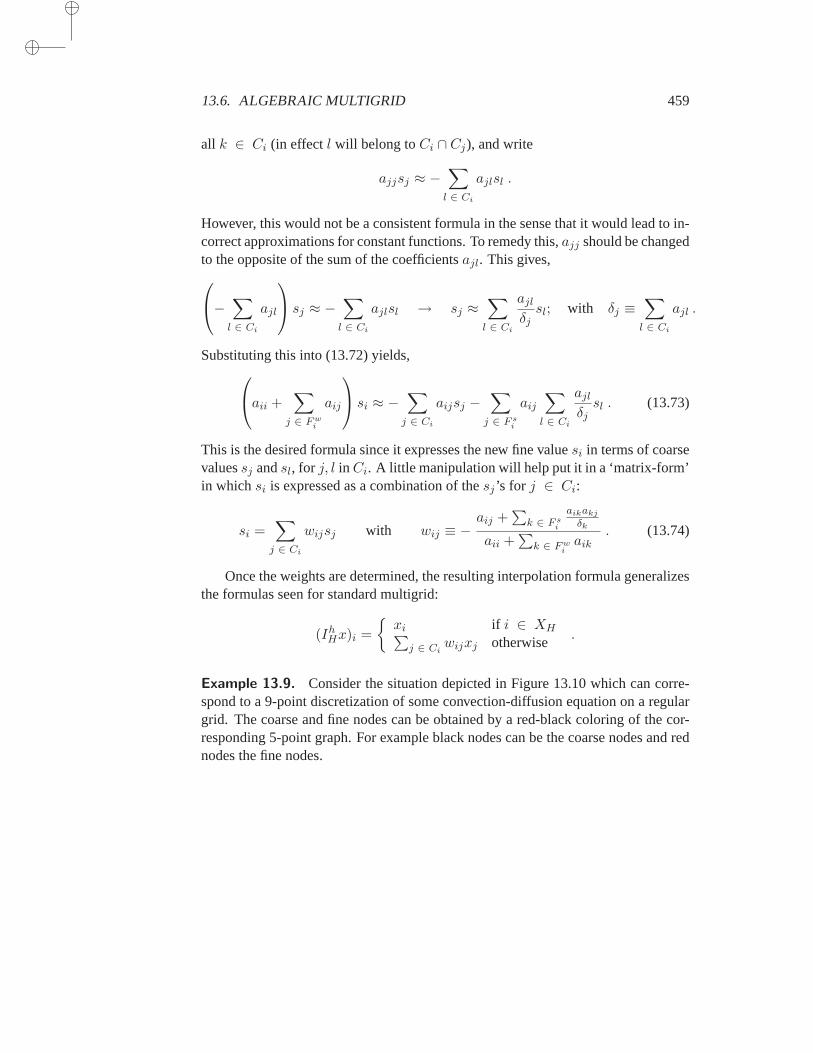
13.6. ALGEBRAIC MULTIGRID 459
all k ∈ Ci (in effectl will belong toCi ∩ Cj), and write
ajjsj ≈ −∑
l ∈ Ci
ajlsl .
However, this would not be a consistent formula in the sense that it would lead to in-correct approximations for constant functions. To remedy this,ajj should be changedto the opposite of the sum of the coefficientsajl. This gives,
−∑
l ∈ Ci
ajl
sj ≈ −∑
l ∈ Ci
ajlsl → sj ≈∑
l ∈ Ci
ajl
δjsl; with δj ≡
∑
l ∈ Ci
ajl .
Substituting this into (13.72) yields,
aii +∑
j ∈ F wi
aij
si ≈ −∑
j ∈ Ci
aijsj −∑
j ∈ F si
aij
∑
l ∈ Ci
ajl
δjsl . (13.73)
This is the desired formula since it expresses the new fine valuesi in terms of coarsevaluessj andsl, for j, l inCi. A little manipulation will help put it in a ‘matrix-form’in whichsi is expressed as a combination of thesj ’s for j ∈ Ci:
si =∑
j ∈ Ci
wijsj with wij ≡ −aij +
∑
k ∈ F si
aikakj
δk
aii +∑
k ∈ F wiaik
. (13.74)
Once the weights are determined, the resulting interpolation formula generalizesthe formulas seen for standard multigrid:
(IhHx)i =
xi if i ∈ XH∑
j ∈ Ciwijxj otherwise
.
Example 13.9. Consider the situation depicted in Figure 13.10 which can corre-spond to a 9-point discretization of some convection-diffusion equation ona regulargrid. The coarse and fine nodes can be obtained by a red-black coloringof the cor-responding 5-point graph. For example black nodes can be the coarsenodes and rednodes the fine nodes.
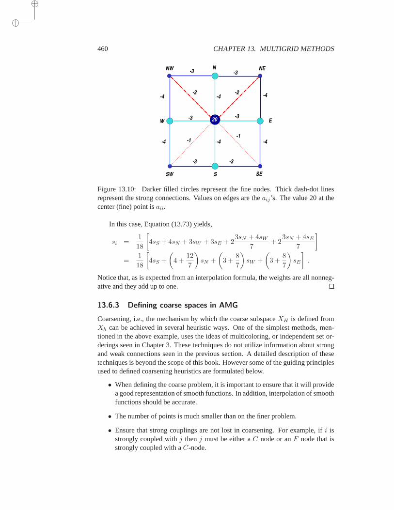
460 CHAPTER 13. MULTIGRID METHODS
W
N
SE
-3 -3
-3-3
-3 -3
-4 -4-4 -1-1
SW S
E
NENW
-2 -2-4-4 -4
20
Figure 13.10: Darker filled circles represent the fine nodes. Thick dash-dot linesrepresent the strong connections. Values on edges are theaij ’s. The value 20 at thecenter (fine) point isaii.
In this case, Equation (13.73) yields,
si =1
18
[
4sS + 4sN + 3sW + 3sE + 23sN + 4sW
7+ 2
3sN + 4sE
7
]
=1
18
[
4sS +
(
4 +12
7
)
sN +
(
3 +8
7
)
sW +
(
3 +8
7
)
sE
]
.
Notice that, as is expected from an interpolation formula, the weights are all nonneg-ative and they add up to one.
13.6.3 Defining coarse spaces in AMG
Coarsening, i.e., the mechanism by which the coarse subspaceXH is defined fromXh can be achieved in several heuristic ways. One of the simplest methods, men-tioned in the above example, uses the ideas of multicoloring, or independent set or-derings seen in Chapter 3. These techniques do not utilize information about strongand weak connections seen in the previous section. A detailed description of thesetechniques is beyond the scope of this book. However some of the guiding principlesused to defined coarsening heuristics are formulated below.
• When defining the coarse problem, it is important to ensure that it will providea good representation of smooth functions. In addition, interpolation of smoothfunctions should be accurate.
• The number of points is much smaller than on the finer problem.
• Ensure that strong couplings are not lost in coarsening. For example, ifi isstrongly coupled withj thenj must be either aC node or anF node that isstrongly coupled with aC-node.

13.6. ALGEBRAIC MULTIGRID 461
• The process should reach a balance between the size ofXH and the accuracyof the interpolation/ restriction functions.
13.6.4 AMG via Multilevel ILU
It was stated in the introduction of this section that the main ingredients needed fordefining an Algebraic Multigrid method are a coarsening scheme and an interpola-tion operator. A number of techniques have been recently developed which attemptto use the framework of incomplete factorizations to define AMG preconditioners.Let us consider coarsening first. Coarsening can be achieved by using variations ofindependent set orderings which were covered in Chapter 3. Often theindependentset is called the fine set and the complement is the coarse set, though this namingisnow somewhat arbitrary.
Recall that independent set orderings transform the original linear system into asystem of the form (
B FE C
)(x
y
)
=
(f
g
)
(13.75)
in which theB block is a diagonal matrix. A block LU factorization will help estab-lish the link with AMG-type methods.
(B FE C
)
=
(I 0
EB−1 I
)(B F0 S
)
whereS is the Schur complement,
S = C − EB−1F .
The above factorization, using independent sets, was at the basis of theILU factoriza-tion with Multi-elimination (ILUM) seen in Chapter 12. Since the Schur complementmatrixS is sparse and the above procedure can be repeated recursively fora few lev-els. Clearly, dropping is applied each time to prune the Schur complementS whichbecomes denser as the number of levels increases. In this section we consider thisfactorization again from the angle of AMG and will define block generalizations.
No Coupling
Figure 13.11: Group- (or Block-) -Independent sets.
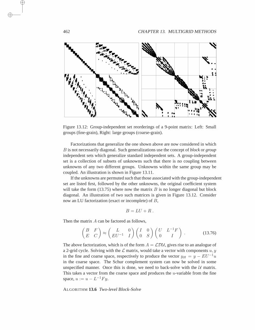
462 CHAPTER 13. MULTIGRID METHODS
Figure 13.12: Group-independent set reorderings of a 9-point matrix: Left: Smallgroups (fine-grain), Right: large groups (coarse-grain).
Factorizations that generalize the one shown above are now consideredin whichB is not necessarily diagonal. Such generalizations use the concept ofblockor groupindependent sets which generalize standard independent sets. A group-independentset is a collection of subsets of unknowns such that there is no coupling betweenunknowns of any two different groups. Unknowns within the same groupmay becoupled. An illustration is shown in Figure 13.11.
If the unknowns are permuted such that those associated with the group-independentset are listed first, followed by the other unknowns, the original coefficient systemwill take the form (13.75) where now the matrixB is no longer diagonal but blockdiagonal. An illustration of two such matrices is given in Figure 13.12. Considernow an LU factorization (exact or incomplete) ofB,
B = LU +R .
Then the matrixA can be factored as follows,(B FE C
)
≈(
L 0EU−1 I
)(I 00 S
)(U L−1F0 I
)
. (13.76)
The above factorization, which is of the formA = LDU , gives rise to an analogue ofa 2-grid cycle. Solving with theLmatrix, would take a vector with componentsu, yin the fine and coarse space, respectively to produce the vectoryH = y − EU−1uin the coarse space. The Schur complement system can now be solved in someunspecified manner. Once this is done, we need to back-solve with theU matrix.This takes a vector from the coarse space and produces theu-variable from the finespace,u := u− L−1Fy.
ALGORITHM 13.6 Two-level Block-Solve
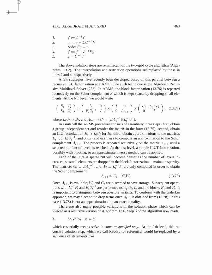
13.6. ALGEBRAIC MULTIGRID 463
1. f := L−1f2. g := g − EU−1f1
3. SolveSy = g4. f := f − L−1Fy5. x = U−1f
The above solution steps are reminiscent of the two-grid cycle algorithm (Algo-rithm 13.2). The interpolation and restriction operations are replaced by those inlines 2 and 4, respectively.
A few strategies have recently been developed based on this parallel between arecursive ILU factorization and AMG. One such technique is the Algebraic Recur-sive Multilevel Solver [253]. In ARMS, the block factorization (13.76) is repeatedrecursively on the Schur complementS which is kept sparse by dropping small ele-ments. At thel-th level, we would write(Bl Fl
El Cl
)
≈(
Ll 0
ElU−1l I
)
×(I 00 Al+1
)
×(Ul L−1
l Fl
0 I
)
, (13.77)
whereLlUl ≈ Bl, andAl+1 ≈ Cl − (ElU−1l )(L−1
l Fl).In a nutshell the ARMS procedure consists of essentially three steps: first, obtain
a group-independent set and reorder the matrix in the form (13.75); second, obtainan ILU factorizationBl ≈ LlUl for Bl; third, obtain approximations to the matricesL−1
l Fl, ElU−1l , andAl+1, and use these to compute an approximation to the Schur
complementAl+1. The process is repeated recursively on the matrixAl+1 until aselected number of levels is reached. At the last level, a simple ILUT factorization,possibly with pivoting, or an approximate inverse method can be applied.
Each of theAi’s is sparse but will become denser as the number of levels in-creases, so small elements are dropped in the block factorization to maintain sparsity.The matricesGl ≡ ElU
−1l , andWl ≡ L−1
l Fl are only computed in order to obtainthe Schur complement
Al+1 ≈ Cl −GlWl. (13.78)
OnceAl+1 is available,Wl andGl are discarded to save storage. Subsequent opera-tions withL−1
l Fl andElU−1l are performed usingUl, Ll and the blocksEl andFl. It
is important to distinguish between possible variants. To conform with the Galerkinapproach, we may elect not to drop terms onceAl+1 is obtained from (13.78). In thiscase (13.78) is not an approximation but an exact equality.
There are also many possible variations in the solution phase which can beviewed as a recursive version of Algorithm 13.6. Step 3 of the algorithm now reads
3. SolveAl+1yl = gl
which essentially meanssolve in some unspecified way. At the l-th level, this re-cursive solution step, which we call RSolve for reference, would be replaced by asequence of statements like

464 CHAPTER 13. MULTIGRID METHODS
3.0 If lev = last3.1 SolveAl+1yl = gl
3.2 Else3.3 RSolve (Al+1, gl)3.4 End
Iterative processes can be used in step 3.3. The preconditioner for thisiterative pro-cess can, for example, be defined using the next,(l+ 2)-th level (without iterating ateach level). This is the simplest approach. It is also possible to use an iterative proce-dure at each level preconditioned (recursively) with the ARMS preconditioner belowthat level. This variation leads to a procedure similar the MG-cycle, if the numberof stepsγ is specificed. Finally, the localBl block can be used to precondition thesystem of thel-th level.
13.7 Multigrid vs Krylov methods
The main differences between preconditioned Krylov subspace methods and themultigrid approach may now have become clearer to the reader. In broef, Krylovmethods take a matrixA and a right-hand sideb and try to produce a solution, usingno other information. The termblack boxis often used for those methods which re-quire minimal input from the user, a good example being that of sparse direct solvers.Preconditioned Krylov subspace methods attempt to duplicate this attribute of directsolvers, but they are not ‘black-box’ solvers since they require parameters and do notalways succeed in solving the problem.
The approach taken by Multigrid methods is to tackle the original problem, e.g.the PDE, directly instead. By doing so, it is possible to exploit properties which arenot always readily available from the dataA, b. For example, what makes multigridwork in the Poisson equation case, is the strong relation between eigenfunctions ofthe iteration matrixM and the mesh. It is this strong relation that makes it possibleto take advantage of coarser meshes and to exploit a divide-and-conquer principlebased on the spectral decomposition ofM . AMG methods try to recover similarrelationships directly fromA, but this is not always easy.
The answer to the question “which method to use?”, cannot be a simple one be-cause it is related to two other important and subjective considerations. Thefirst isthe cost of the coding effort. Whether or not one is willing to spend a substantialamount of time coding and testing, is now a factor. The second is how importantit isto develop an “optimal” code for the problem at hand. If the goal is to solve asinglelinear system then a direct solver (assuming enough memory is available) or a pre-conditioned Krylov solver (in case memory is an issue) may be best. Here, optimalityis a secondary consideration. On the other extreme, the best possible performancemay be required from the solver if it is meant to be part of a large simulation codewhich may take, say, days on a high-performance computer to complete one run. Inthis case, it may be worth the time and cost to build the best solver possible, becausethis cost will be amortized over the lifetime of the simulation code. Here, multi-level techniques can constitute a significant part of the solution scheme. A wide grey
13.7. MULTIGRID VS KRYLOV METHODS 465
zone lies in between these two extremes wherein Krylov subspace methods are ofteninvoked.
It may be important to comment on another practical consideration, which is thatmost industrial solvers are not monolithic schemes based on one single approach.Rather, they are comprised of building blocks which include tools extracted fromvarious methodologies: direct sparse techniques, multilevel methods, ILU type pre-conditioners, as well as strategies that exploit the specificity of the problem.Forexample, a solver could utilize the knowledge of the problem to reduce the systemby eliminating part of the unknowns, then invoke an AMG or multigrid scheme tosolve the resulting reduced system in cases when it is known to be Poisson-like and anILU-Krylov approach combined with some reordering schemes (from sparse directsolvers) in other cases. Good iterative solvers must rely on a battery of techniquesif they are to be robust and efficient at the same time. To ensure robustness, indus-trial codes may include an option to resort to direct solvers for those, hopefully rare,instances when the main iterative scheme fails.
PROBLEMS
P-13.1 The following notation will be used. Given a vectorz of sizen.m denote by
Z = [z]n,m
the matrix of dimensionn ×m with entriesZij = z(j−1)∗n+i. When there is no ambiguitythe subscriptsn,m are omitted. In other wordsn consecutive entries ofz will form thecolumns ofZ. The opposite operation, which consists of stacking the consecutive columnsof a matrixZ into a vectorz, is denoted by
z = Z| .
a. Letu ∈ Rm, v ∈ R
n. What is the matrixZ = [z]n,m whenz = u⊗ v?
b. Show that
(I ⊗A)z = (A.[z])| and (A⊗ I)z =([z].AT
)
|
c. Show, more generally, that
(A⊗B)z =(B.[z].AT
)
|
d. What becomes of the above relation whenz = u ⊗ v? Find an eigenvector ofA ⊗ Bbased on this.
e. Show that(A⊗B)T = (AT ⊗BT ).
P-13.2 Establish that the eigenvectors of the Gauss-Seidel operator given by (13.29) areindeed a set ofn linearly independent vectors. (Hint: notice that the eigenvalues other thanfor k = (n + 1)/2 are all double, it suffices to show that the two eigenvectors defined bythe formula are independent.) What happens if the absolute values are removed from theexpression (13.29)?
466 CHAPTER 13. MULTIGRID METHODS
P-13.3 Consider the Gauss-Seidel iteration as a smoother for the 1-D model problem, whenn = 11 (spectrum illustrated in Figure 13.4.) For each eigenvector ui of the original matrixA, compute the norm reduction‖Gui‖/‖ui‖, whereG is the Gauss-Seidel iteration matrix.Plot these ratios againsti, in a way that is similar to Figure 13.4. What can you conclude?Repeat for the powersG2, andG4, andG8. What can you conclude (see the statement madeat end of Section 13.2.3)?
P-13.4 Show relation (13.31). Consider as an example, a7 × 5 grid and illustrate for thiscase the semi-interpolation operatorsIh
x,2h andIhy,2h. Then derive the relation by seeing how
the 2-D interpolation operator was defined in Section 13.3.1.
P-13.5 Show the relation (13.38). Consider first as an example, a7 × 5 grid and illustratefor this case the semi-restriction operatorsI2h
x,h and I2hy,h. Then use (13.31) (see previous
exercise) and part (e) of Exercise 1.
P-13.6 What is the matrixIHh AhI
hH for the 2-D model problem when Full Weighting is
used? [Hint: Use the tensor product notation and the resultsof Exercises 5 and 4.]
P-13.7 Consider the matrixJω given by (13.20). Show that it is possible to findω > 1 suchthatρ(Jω) > 1. Similar question forω < 0.
P-13.8 Derive the full weighting formula by applying the trapezoidal rule to approximatethe numerator and denominator in the following approximation:
u(x) ≈∫ x+h
x−hu(t)dt
∫ x+h
x−h1.dt
.
P-13.9 Derive theB-form (or preconditioning form, see (13.41)) of the weighted Jacobiiteration.
P-13.10 Do the following experiment using an interactive package such as Matlab - (orcode in FORTRAN or C). Consider the linear systemAx = 0 whereA arises from thediscretization of−u′′ on [0, 1] using 64 internal points. Takeu0 to be the average of the twomodesun/4 = u16 andu3n/4 = u48. Plot the initial error (Hint: the error is justu0), then theerror after 2 steps of the Richardson process, then the errorafter 5 steps of the Richardsonprocess. Plot also the components of the final error after the5 Richardson steps, with respectto the eigenbasis. Now obtain the residual on the gridΩ2h, and plot the residual obtainedafter 2 and 5 Richardson steps on the coarse-grid problem. Show also the components of theerror in the eigenbasis of the original problem (on the fine mesh). Finally, interpolate to thefine grid and repeat the process again, doing 2 and then 5 stepsof the Richardson process.
P-13.11 Repeat Exercise 10 using the Gauss-Seidel iteration instead of the Richardson iter-ation.
P-13.12 Consider the cost of the general MG algorithm as given by the recurrence formula(13.46). Solve the recurrence equation (in terms ofη andγ) for the 1-D case. You mayassume thatn = 2k + 1 and that the maximum number of levels are used so that the costofthe last system to solve is zero. For the 2-D case, you may assume thatn = m = 2k + 1.Under which condition is the costO(n log n) wheren is the size of the finest grid underconsideration? What would be the situation for 3-D problems?
P-13.13 It was stated in Section 13.4.4 that condition (13.48) implies the condition (13.49)provided an assumption is made on the interpolationIh
H . Prove a rigorous bound of the type(13.49) (i.e., findc1) by assuming the conditions (13.48) (13.51) and
‖u− IhHu‖ ≤ c4hκ
13.7. MULTIGRID VS KRYLOV METHODS 467
in which as beforeu represents the discretization of the the solution of the continuous prob-lem (i.e., the continuous solution sampled at the grid points ofΩh or ΩH ).
P-13.14 Justify the definition of the norm‖v‖h in Example 13.6 by considering that theintegral
∫ 1
0
v(t)2 dt
is approximated by the Trapezoidal rule. It is assumed thatv(x0) = v(xn+1) = 0 and thecomposite trapezoidal rule uses all pointsx0, . . . , xn+1.
P-13.15 Find the constantα in the smoothing property (13.62), for the case of Richardon’siteration whenA is SPD. [Hint: Richardson’s iteration is like a Jacobi iteration where thediagonal is replaced by the identity.]
P-13.16 Extend the argument of Example 13.6 to the 2-D case. Start with the case ofthe square(0, 1)2 which uses the same discretization in each direction. Then consider themore general situation. Define the norm‖v‖h from the discreteL2 norm (see also previousexercise).
P-13.17 Establish a bound of the type shown in Example 13.6 using the 2-norm instead ofthe discreteL2 norm. What if theAh norm is used?
P-13.18 The energy norm can be used to establish a result similar to that of Theorem 13.2leading to a slightly simpler argument. It is now assumed that (13.49) is satisfied with respectto theAh-norm, i.e., that
‖uh − IhHu
H‖Ah≤ c1hκ .
a. Show that for any vectorv in ΩH we have
‖IhHv‖Ah
= ‖v‖AH.
b. Letuh0 the initial guess at gridΩh in FMG and assume that the error achieved by the
system at levelH = 2h satisfies‖uH − uH‖AH≤ c1c3H
κ, in which c3 is to bedetermined. Follow the argument of the proof of Theorem (13.2) and use the relationestablished in (a) to show that
‖uh − uh0‖Ah
≤ ‖uh − IhHu
H‖Ah+ ‖uH − uH‖AH
≤ c1hκ + c1c3Hκ .
c. Show a result analogous to that of Theorem 13.2 which uses theAh-norm, i.e., findc3such that‖uh − uh‖Ah
≤ c1c3hκ, on each grid.
P-13.19 Starting from the relation (13.73), establish (13.74).
NOTES AND REFERENCES. The material presented in this chapter is based on several sources. Fore-most among these are the references [65, 207, 163, 286, 301]. A highly recommended reference is the“Multigrid tutorial, second edition” by Briggs, Van Hansen, and Mc Cormick[65], for its excellentintroduction to the subject. This tutorial includes enough theory to understand how multigrid meth-ods work. More detailed volumes include the books by Mc Cormick et al. [207], Hackbusch [162],Hackbusch [163], Wesseling [311], and the more recent book by Trottenberg and al. [286].
Early work on multigrid methods dates back to the 1960s and includes the papers by Brakhage [46],Fedorenko [124, 125], Bakhvalov [23], and Kronsjo and Dahlquist [193]. However, Multigrid meth-ods have seen much of their modern development in the 1970s and early1980s, essentially under thepioneering work of Brandt [54, 55, 56]. Brandt played a key role in promoting the use of MG by estab-lishing their overwhelming superiority over existing techniques for elliptic PDEs and by introducing
468 CHAPTER 13. MULTIGRID METHODS
many new concepts which are now widely use in MG literature. Algebraic multigrid methods werelater developed to attempt to obtain similar performance. These methods were introduced in [58] andanalyzed in a number of papers, see e.g., [57, 235].
Closely related to the multigrid approach is the Aggregation-Disaggregation technique which ispopular in Markov chain modeling. A recommended book for these methods and others used in thecontext of Markov chain modeling is [275].
Today MG methods are still among the most efficient techniques available for solving EllipticPDEs on regularly structured problems. Their Algebraic variants do notseem to have proven as ef-fective and the search for the elusive “black-box” iterative solver is still under way, with research onmultilevel methods in general and AMG in particular still quite active. With computer power con-stantly improving, problems are becoming larger and more complex, andthis makes mesh-independentconvergence look ever more attractive.
The paper [253] describes a scalar version of the Algebraic Recursive Multilevel Solver and thereport [203] describes a parallel implementation. The related method named MLILU described in [28]also exploits the connection between ILU and AMG. The parallel version ofARMS (called pARMS)is available from the author’s web site:www.cs.umn.edu/∼saad.
Resources for Multigrid are available inwww.mgnet.org which provides bibliographical refer-ences, software, and a newsletter. In particular, Examples 13.4 and 13.5 have been run with theMGLAB matlab codes (contributed by James Bordner and Faisal Saied) available from this site. Aparallel code named HYPRE which is available from the Lawrence Livermore National Lab, includesimplementations of AMG.
Chapter 14
DOMAIN DECOMPOSITION METHODS
As multiprocessing technology is steadily gaining ground, new classes of numerical methods
that can take better advantage of parallelism are emerging. Among these techniques, domain
decomposition methods are undoubtedly the best known and perhaps the most promising for
certain types of problems. These methods combine ideas from Partial Differential Equations,
linear algebra, mathematical analysis, and techniques from graph theory. This chapter is devoted
to “decomposition” methods, which are based on the general concepts of graph partitionings.
14.1 Introduction
Domain decomposition methods refer to a collection of techniques which revolvearound the principle of divide-and-conquer. Such methods have beenprimarily de-veloped for solving Partial Differential Equations over regions in two or three dimen-sions. However, similar principles have been exploited in other contexts of scienceand engineering. In fact, one of the earliest practical uses for domain decompositionapproaches was in structural engineering, a discipline which is not dominated by Par-tial Differential Equations. Although this chapter considers these techniques from apurely linear algebra view-point, the basic concepts, as well as the terminology, areintroduced from a model Partial Differential Equation.
Consider the problem of solving the Laplace Equation on an L-shaped domainΩ partitioned as shown in Figure 14.1. Domain decomposition or substructuringmethods attempt to solve the problem on the entire domain
Ω =s⋃
i=1
Ωi,
from problem solutions on the subdomainsΩi. There are several reasons why suchtechniques can be advantageous. In the case of the above picture, oneobvious rea-son is that the subproblems are much simpler because of their rectangular geometry.For example, fast Poisson solvers can be used on each subdomain in this case. Asecond reason is that the physical problem can sometimes be split naturally into asmall number of subregions where the modeling equations are different (e.g., Euler’sequations on one region and Navier-Stokes in another).
Substructuring can also be used to develop “out-of-core” solution techniques.As already mentioned, such techniques were often used in the past to analyze very
469
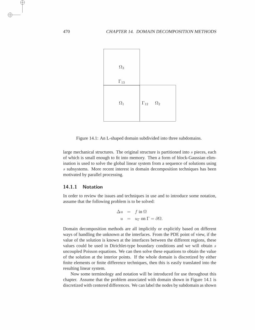
470 CHAPTER 14. DOMAIN DECOMPOSITION METHODS
Ω1 Ω2
Ω3
Γ12
Γ13
Figure 14.1: An L-shaped domain subdivided into three subdomains.
large mechanical structures. The original structure is partitioned intos pieces, eachof which is small enough to fit into memory. Then a form of block-Gaussian elim-ination is used to solve the global linear system from a sequence of solutionsusings subsystems. More recent interest in domain decomposition techniques has beenmotivated by parallel processing.
14.1.1 Notation
In order to review the issues and techniques in use and to introduce some notation,assume that the following problem is to be solved:
∆u = f in Ω
u = uΓ onΓ = ∂Ω.
Domain decomposition methods are all implicitly or explicitly based on differentways of handling the unknown at the interfaces. From the PDE point of view, if thevalue of the solution is known at the interfaces between the different regions, thesevalues could be used in Dirichlet-type boundary conditions and we will obtainsuncoupled Poisson equations. We can then solve these equations to obtain the valueof the solution at the interior points. If the whole domain is discretized by eitherfinite elements or finite difference techniques, then this is easily translated into theresulting linear system.
Now some terminology and notation will be introduced for use throughout thischapter. Assume that the problem associated with domain shown in Figure 14.1isdiscretized with centered differences. We can label the nodes by subdomain as shown
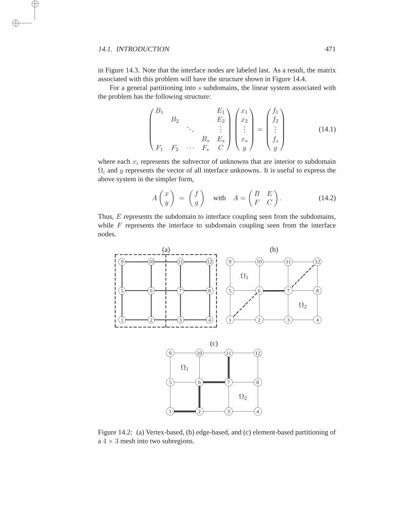
14.1. INTRODUCTION 471
in Figure 14.3. Note that the interface nodes are labeled last. As a result, thematrixassociated with this problem will have the structure shown in Figure 14.4.
For a general partitioning intos subdomains, the linear system associated withthe problem has the following structure:
B1 E1
B2 E2.. .
...Bs Es
F1 F2 · · · Fs C
x1
x2...xs
y
=
f1
f2...fs
g
(14.1)
where eachxi represents the subvector of unknowns that are interior to subdomainΩi andy represents the vector of all interface unknowns. It is useful to express theabove system in the simpler form,
A
(xy
)
=
(fg
)
with A =
(B EF C
)
. (14.2)
Thus,E represents the subdomain to interface coupling seen from the subdomains,while F represents the interface to subdomain coupling seen from the interfacenodes.
1 2 3 4
5 6 7 8
9 10 11 12
(a)
1 2 3 4
5 6 7 8
9 10 11 12
Ω1
Ω2
(b)
1 2 3 4
5 6 7 8
9 10 11 12
Ω1
Ω2
(c)
Figure 14.2: (a) Vertex-based, (b) edge-based, and (c) element-based partitioning ofa4× 3 mesh into two subregions.
472 CHAPTER 14. DOMAIN DECOMPOSITION METHODS
14.1.2 Types of Partitionings
When partitioning a problem, it is common to use graph representations. Since thesubproblems obtained from a given partitioning will eventually be mapped into dis-tinct processors, there are some restrictions regarding the type of partitioning needed.For example, in Element-By-Element finite element techniques, it may be desirableto map elements into processors instead of vertices. In this case, the restriction meansno element should be split between two subdomains, i.e., all information related toa given element is mapped to the same processor. These partitionings are termedelement-based. A somewhat less restrictive class of partitionings are the edge-basedpartitionings, which do not allow edges to be split between two subdomains. Thesemay be useful for finite volume techniques where computations are expressed interms of fluxes across edges in two dimensions. Finally, vertex-based partitioningswork by dividing the origin vertex set into subsets of vertices and have norestrictionson the edges, i.e., they allow edges or elements to straddle between subdomains. SeeFigure 14.2, (a), (b), and (c).
14.1.3 Types of Techniques
The interface values can be obtained by employing a form of block-Gaussian elimi-nation which may be too expensive for large problems. In some simple cases,usingFFT’s, it is possible to explicitly obtain the solution of the problem on the interfacesinexpensively.
Other methods alternate between the subdomains, solving a new problem eachtime, with boundary conditions updated from the most recent subdomain solutions.These methods are calledSchwarz Alternating Procedures, after the Swiss math-ematician who used the idea to prove the existence for a solution of the Dirichletproblem on irregular regions.
The subdomains may be allowed tooverlap. This means that theΩi’s are suchthat
Ω =⋃
i=1,s
Ωi, Ωi ∩ Ωj 6= φ.
For a discretized problem, it is typical to quantify the extent of overlapping by thenumber of mesh-lines that are common to the two subdomains. In the particular caseof Figure 14.3, the overlap is of order one.
The various domain decomposition techniques are distinguished by four features:
1. Type of Partitioning.For example, should partitioning occur along edges, oralong vertices, or by elements? Is the union of the subdomains equal to theoriginal domain or a superset of it (fictitious domain methods)?
2. Overlap.Should sub-domains overlap or not, and by how much?
3. Processing of interface values.For example, is the Schur complement ap-proach used? Should there be successive updates to the interface values?
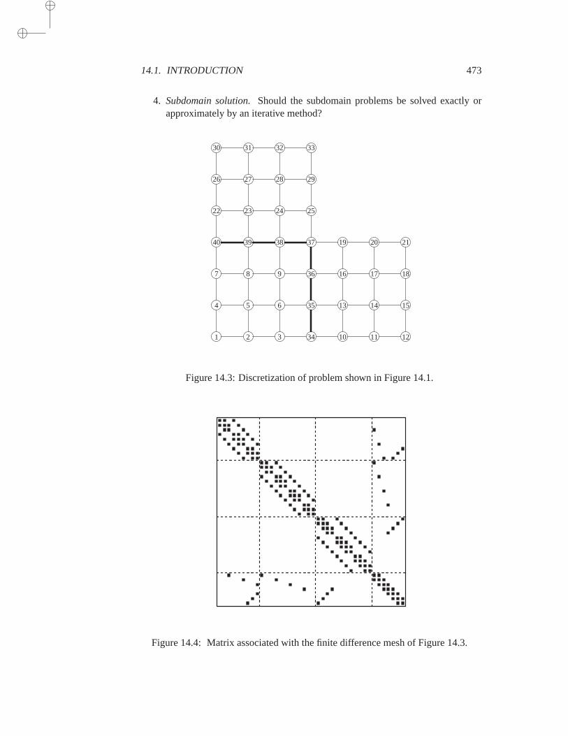
14.1. INTRODUCTION 473
4. Subdomain solution.Should the subdomain problems be solved exactly orapproximately by an iterative method?
1 2 3
4 5 6
7 8 9
10 11 12
13 14 15
16 17 18
19 20 21
22 23 24 25
26 27 28 29
30 31 32 33
34
35
36
37383940
Figure 14.3: Discretization of problem shown in Figure 14.1.
Figure 14.4: Matrix associated with the finite difference mesh of Figure 14.3.

474 CHAPTER 14. DOMAIN DECOMPOSITION METHODS
The methods to be discussed in this chapter will be classified in four distinctgroups. First, direct methods and the substructuring approach are useful for intro-ducing some definitions and for providing practical insight. Second, amongthe sim-plest and oldest techniques are the Schwarz Alternating Procedures. Then, there aremethods based on preconditioning the Schur complement system. The last categorygroups all the methods based on solving the linear system with the matrixA, by usinga preconditioning derived from Domain Decomposition concepts.
14.2 Direct Solution and the Schur Complement
One of the first divide-and-conquer ideas used in structural analysisexploited thepartitioning (14.1) in a direct solution framework. This approach, which is coveredin this section, introduces the Schur complement and explains some of its properties.
14.2.1 Block Gaussian Elimination
Consider the linear system written in the form (14.2), in whichB is assumed to benonsingular. From the first equation the unknownx can be expressed as
x = B−1(f − Ey). (14.3)
Upon substituting this into the second equation, the followingreduced systemis ob-tained:
(C − FB−1E)y = g − FB−1f. (14.4)
The matrixS = C − FB−1E (14.5)
is called theSchur complementmatrix associated with they variable. If this matrixcan be formed and the linear system (14.4) can be solved, all the interfacevariablesy will become available. Once these variables are known, the remaining unknownscan be computed, via (14.3). Because of the particular structure ofB, observe thatany linear system solution with it decouples ins separate systems. The parallelismin this situation arises from this natural decoupling.
A solution method based on this approach involves four steps:
1. Obtain the right-hand side of the reduced system (14.4).
2. Form the Schur complement matrix (14.5).
3. Solve the reduced system (14.4).
4. Back-substitute using (14.3) to obtain the other unknowns.
One linear system solution with the matrixB can be saved by reformulating thealgorithm in a more elegant form. Define
E′ = B−1E and f ′ = B−1f.
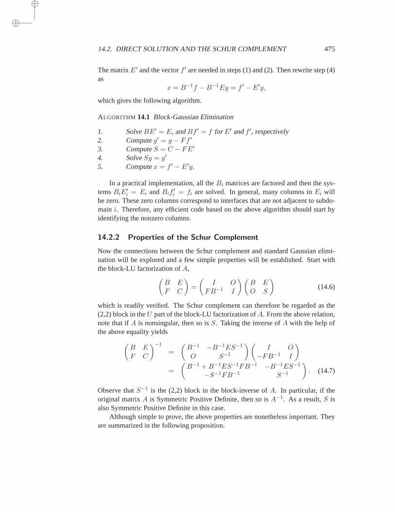
14.2. DIRECT SOLUTION AND THE SCHUR COMPLEMENT 475
The matrixE′ and the vectorf ′ are needed in steps (1) and (2). Then rewrite step (4)as
x = B−1f −B−1Ey = f ′ − E′y,
which gives the following algorithm.
ALGORITHM 14.1 Block-Gaussian Elimination
1. SolveBE′ = E, andBf ′ = f for E′ andf ′, respectively2. Computeg′ = g − Ff ′3. ComputeS = C − FE′
4. SolveSy = g′
5. Computex = f ′ − E′y.
In a practical implementation, all theBi matrices are factored and then the sys-temsBiE
′i = Ei andBif
′i = fi are solved. In general, many columns inEi will
be zero. These zero columns correspond to interfaces that are not adjacent to subdo-main i. Therefore, any efficient code based on the above algorithm should start byidentifying the nonzero columns.
14.2.2 Properties of the Schur Complement
Now the connections between the Schur complement and standard Gaussianelimi-nation will be explored and a few simple properties will be established. Start withthe block-LU factorization ofA,
(B EF C
)
=
(I O
FB−1 I
)(B EO S
)
(14.6)
which is readily verified. The Schur complement can therefore be regarded as the(2,2) block in theU part of the block-LU factorization ofA. From the above relation,note that ifA is nonsingular, then so isS. Taking the inverse ofA with the help ofthe above equality yields
(B EF C
)−1
=
(B−1 −B−1ES−1
O S−1
)(I O
−FB−1 I
)
=
(B−1 +B−1ES−1FB−1 −B−1ES−1
−S−1FB−1 S−1
)
. (14.7)
Observe thatS−1 is the (2,2) block in the block-inverse ofA. In particular, if theoriginal matrixA is Symmetric Positive Definite, then so isA−1. As a result,S isalso Symmetric Positive Definite in this case.
Although simple to prove, the above properties are nonetheless important. Theyare summarized in the following proposition.
476 CHAPTER 14. DOMAIN DECOMPOSITION METHODS
Proposition 14.1 LetA be a nonsingular matrix partitioned as in (14.2) and suchthat the submatrixB is nonsingular and letRy be the restriction operator onto theinterface variables, i.e, the linear operator defined by
Ry
(xy
)
= y.
Then the following properties are true.
1. The Schur complement matrixS is nonsingular.
2. IfA is SPD, then so isS.
3. For anyy, S−1y = RyA−1(
0y
)
.
The first property indicates that a method that uses the above block Gaussianelimination algorithm is feasible sinceS is nonsingular. A consequence of the sec-ond property is that whenA is positive definite, an algorithm such as the ConjugateGradient algorithm can be used to solve the reduced system (14.4). Finally, the thirdproperty establishes a relation which may allow preconditioners forS to be definedbased on solution techniques with the matrixA.
14.2.3 Schur Complement for Vertex-Based Partitionings
The partitioning used in Figure 14.3 is edge-based, meaning that a given edge in thegraph does not straddle two subdomains, or that if two vertices are coupled, then theycannot belong to the two distinct subdomains. From the graph theory point of view,this is perhaps less common than vertex-based partitionings in which a vertex isnotshared by two partitions (except when domains overlap). A vertex-based partitioningis illustrated in Figure 14.5.
We will call interface edges all edges that link vertices that do not belong tothesame subdomain. In the case of overlapping, this needs clarification. An overlappingedge or vertex belongs to the same subdomain. Interface edges are only those thatlink a vertex to another vertex which is not in the same subdomain already, whether inthe overlapping portion or elsewhere. Interface vertices are those vertices in a givensubdomain that are adjacent to an interface edge. For the example of the figure, theinterface vertices for subdomain one (bottom, left subsquare) are the vertices labeled10 to 16. The matrix shown at the bottom of Figure 14.5 differs from the one ofFigure 14.4, because here the interface nodes are not relabeled the last in the globallabeling as was done in Figure 14.3. Instead, the interface nodes are labeled as thelast nodes in each subdomain. The number of interface nodes is about twice that ofthe edge-based partitioning.
Consider the Schur complement system obtained with this new labeling. It canbe written similar to the edge-based case using a reordering in which all interfacevariables are listed last. The matrix associated with the domain partitioning of thevariables will have a naturals-block structure wheres is the number of subdomains.
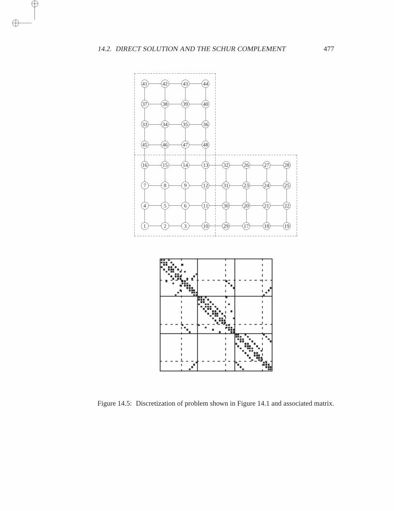
14.2. DIRECT SOLUTION AND THE SCHUR COMPLEMENT 477
1 2 3
4 5 6
7 8 9
10
11
12
13141516
17 18 19
20 21 22
23 24 25
26 27 28
29
30
31
32
33 34 35 36
37 38 39 40
41 42 43 44
45 46 47 48
Figure 14.5: Discretization of problem shown in Figure 14.1 and associatedmatrix.
478 CHAPTER 14. DOMAIN DECOMPOSITION METHODS
For example, whens = 3 (as is the case in the above illustration), the matrix has theblock structure defined by the solid lines in the figure, i.e.,
A =
A1 A12 A13
A21 A2 A23
A31 A32 A3
. (14.8)
In each subdomain, the variables are of the form
zi =
(xi
yi
)
,
wherexi denotes interior nodes whileyi denotes the interface nodes associated withsubdomaini. Each matrixAi will be called the local matrix.
The structure ofAi is as follows:
Ai =
(Bi Ei
Fi Ci
)
(14.9)
in which, as before,Bi represents the matrix associated with the internal nodes ofsubdomaini andEi andFi represent the couplings to/from local interface nodes. ThematrixCi is the local part of the interface matrixC defined before, and represents thecoupling between local interface points. A careful look at the matrix in Figure 14.5reveals an additional structure for the blocksAij j 6= i. PartitioningAij accordingto the variablesxi, yi on the one hand (rows) andxj , yj on the other, reveals that it iscomprised of only one nonzero block. Indeed, there is no coupling betweenxi andxj , betweenxi andyj , or betweenyi andxj . Therefore, the submatrixAij has thefollowing structure,
Aij =
(0 00 Eij
)
. (14.10)
In addition, most of theEij matrices are zero since only those indicesj of the sub-domains that have couplings with subdomaini will yield a nonzeroEij .
Now write the part of the linear system that is local to subdomaini, as
Bixi + Eiyi = fi
Fixi + Ciyi +∑
j∈NiEijyj = gi
. (14.11)
The termEijyj is the contribution to the equation from the neighboring subdomainnumberj, andNi is the set of subdomains that are adjacent to subdomaini. As-suming thatBi is nonsingular, the variablexi can be eliminated from this system byextracting from the first equationxi = B−1
i (fi − Eiyi) which yields, upon substitu-tion in the second equation,
Siyi +∑
j∈Ni
Eijyj = gi − FiB−1i fi, i = 1, . . . , s (14.12)
in whichSi is the “local” Schur complement
Si = Ci − FiB−1i Ei. (14.13)
14.2. DIRECT SOLUTION AND THE SCHUR COMPLEMENT 479
When written for all subdomainsi, the equations (14.12) yield a system of equationswhich involves only the interface pointsyj , j = 1, 2, . . . , s and which has a naturalblock structure associated with these vector variables
S =
S1 E12 E13 · · · E1s
E21 S2 E23 · · · E2s...
. . ....
.... ..
...Es1 Es2 Es3 · · · Ss
. (14.14)
The diagonal blocks in this system, namely, the matricesSi, are dense in general,but the offdiagonal blocksEij are sparse and most of them are zero. Specifically,Eij 6= 0 only if subdomainsi andj have at least one equation that couples them.
A structure of the global Schur complementS has been unraveled which has thefollowing important implication:For vertex-based partitionings, the Schur comple-ment matrix can be assembled from local Schur complement matrices (theSi’s) andinterface-to-interface information (theEij ’s). The term “assembled” was used onpurpose because a similar idea will be exploited for finite element partitionings.
14.2.4 Schur Complement for Finite-Element Partitionings
In finite-element partitionings, the original discrete setΩ is subdivided intos subsetsΩi, each consisting of a distinct set of elements. Given a finite element discretiza-tion of the domainΩ, a finite dimensional spaceVh of functions overΩ is defined,e.g., functions that are piecewise linear and continuous onΩ, and that vanish on theboundaryΓ of Ω. Consider now the Dirichlet problem onΩ and recall that its weakformulation on the finite element discretization can be stated as follows (see Section2.3):
Find u ∈ Vh such that a(u, v) = (f, v), ∀ v ∈ Vh,
where the bilinear forma(., .) is defined by
a(u, v) =
∫
Ω∇u.∇v dx =
∫
Ω
(∂u
∂x1
∂v
∂x1+
∂u
∂x2
∂u
∂x2
)
dx.
It is interesting to observe that since the set of the elements of the differentΩi’s aredisjoint,a(., .) can be decomposed as
a(u, v) =s∑
i=1
ai(u, v),
whereai(u, v) =
∫
Ωi
∇u.∇v dx.
In fact, this is a generalization of the technique used to assemble the stiffnessma-trix from element matrices, which corresponds to the extreme case where each Ωi
consists of exactly one element.
480 CHAPTER 14. DOMAIN DECOMPOSITION METHODS
If the unknowns are ordered again by subdomains and the interface nodes areplaced last as was done in Section 14.1, immediately the system shows the samestructure,
B1 E1
B2 E2. ..
...Bs Es
F1 F2 · · · Fs C
x1
x2...xs
y
=
f1
f2...fs
g
(14.15)
where eachBi represents the coupling between interior nodes andEi andFi repre-sent the coupling between the interface nodes and the nodes interior toΩi. Note thateach of these matrices has been assembled from element matrices and can thereforebe obtained from contributions over all subdomainΩj that contain any node ofΩi.
In particular, assume that the assembly is considered only with respect toΩi.Then the assembled matrix will have the structure
Ai =
(Bi Ei
Fi Ci
)
,
whereCi contains only contributions from local elements, i.e., elements that are inΩi. Clearly,C is the sum of theCi’s,
C =s∑
i=1
Ci.
The Schur complement associated with the interface variables is such that
S = C − FB−1E
= C −s∑
i=1
FiB−1i Ei
=s∑
i=1
Ci −s∑
i=1
FiB−1i Ei
=s∑
i=1
[Ci − FiB
−1i Ei
].
Therefore, ifSi denotes thelocal Schur complement
Si = Ci − FiB−1i Ei,
then the above proves that,
S =s∑
i=1
Si, (14.16)
showing again that the Schur complement can be obtained easily from smaller Schurcomplement matrices.
14.2. DIRECT SOLUTION AND THE SCHUR COMPLEMENT 481
Another important observation is that the stiffness matrixAk, defined above byrestricting the assembly toΩk, solves a Neumann-Dirichlet problem onΩk. Indeed,consider the problem
(Bk Ek
Fk Ck
) (xk
yk
)
=
(fk
gk
)
. (14.17)
The elements of the submatrixCk are the termsak(φi, φj) whereφi, φj are the basisfunctions associated with nodes belonging to the interfaceΓk. As was stated above,the matrixC is the sum of these submatrices. Consider the problem of solving thePoisson equation onΩk with boundary conditions defined as follows: OnΓk0, thepart of the boundary which belongs toΓk, use the original boundary conditions;on the interfacesΓkj with other subdomains, use a Neumann boundary condition.According to Equation (2.47) seen in Section 2.3, thej-th equation will be of theform, ∫
Ωk
∇u.∇φj dx =
∫
Ωk
fφjdx+
∫
Γk
φj∂u
∂~nds. (14.18)
This gives rise to a system of the form (14.17) in which thegk part of the right-handside incorporates the Neumann data related to the second integral on the right-handside of (14.18).
It is interesting to note that if a problem were to be solved with all-Dirichlet con-ditions, i.e., if the Neumann conditions at the interfaces were replaced by Dirichletconditions, the resulting matrix problem would be of the form,
(Bk Ek
0 I
) (xk
yk
)
=
(fk
gk
)
(14.19)
wheregk represents precisely the Dirichlet data. Indeed, according to what wasseen in Section 2.3, Dirichlet conditions are handled simply by replacing equationsassociated with boundary points by identity equations.
14.2.5 Schur Complement for the model problem
An explicit expression for the Schur complement can be found in the simple case ofa rectangular region partitioned into two sub-domains as illustrated in Figure 14.6.The figure shows a vertex based partitioning but what follows is also valid for edge-based partitionings since we will only compute the local Schur complementsS1, S2
from which the the global Schur complement is constituted. For an edge-based parti-tioning, the Schur complementS is the sum of the local Schur complementsS1 andS2. For a vertex-based partitioning,S is of the form (14.14), withs = 2.
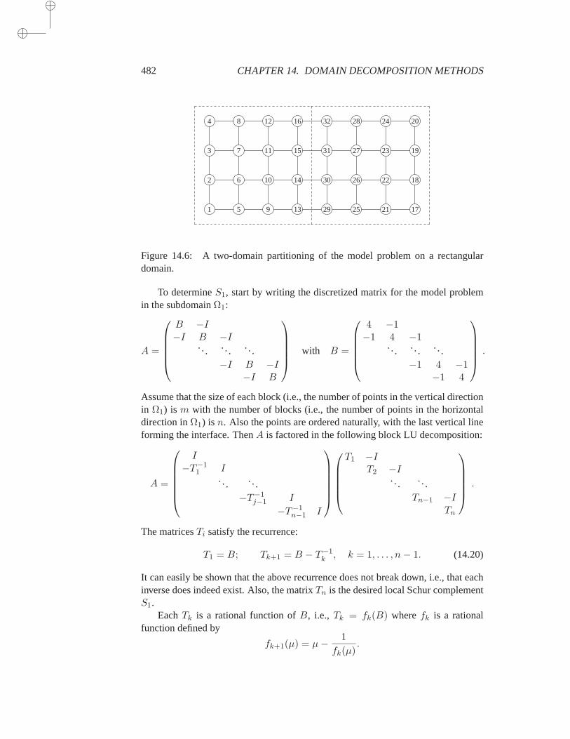
482 CHAPTER 14. DOMAIN DECOMPOSITION METHODS
1 5 9
2 6 10
3 7 11
13
14
15
161284
25 21 17
26 22 1830
27 23 19
28 24 20
29
31
32
Figure 14.6: A two-domain partitioning of the model problem on a rectangulardomain.
To determineS1, start by writing the discretized matrix for the model problemin the subdomainΩ1:
A =
B −I−I B −I
. .. .. . .. .−I B −I
−I B
with B =
4 −1−1 4 −1
. .. . .. . ..−1 4 −1
−1 4
.
Assume that the size of each block (i.e., the number of points in the vertical directionin Ω1) is m with the number of blocks (i.e., the number of points in the horizontaldirection inΩ1) is n. Also the points are ordered naturally, with the last vertical lineforming the interface. ThenA is factored in the following block LU decomposition:
A =
I−T−1
1 I.. . . . .
−T−1j−1 I
−T−1n−1 I
T1 −IT2 −I
. . . . ..Tn−1 −I
Tn
.
The matricesTi satisfy the recurrence:
T1 = B; Tk+1 = B − T−1k , k = 1, . . . , n− 1. (14.20)
It can easily be shown that the above recurrence does not break down, i.e., that eachinverse does indeed exist. Also, the matrixTn is the desired local Schur complementS1.
EachTk is a rational function ofB, i.e., Tk = fk(B) wherefk is a rationalfunction defined by
fk+1(µ) = µ− 1
fk(µ).
14.2. DIRECT SOLUTION AND THE SCHUR COMPLEMENT 483
To each eigenvalueµ of B, is associated an eigenvalueλk. This sequence of eigen-values satisfies the recurrence
λk+1 = µ− 1
λk.
To calculatefn it is sufficient to calculateλk in terms ofµ. The above differenceequation, differs from the ones we have encountered in other chapters, in that it isnonlinear. It can be solved by defining the auxiliarly unknown
ηk =k∏
j=0
λj .
By definitionλ0 = 1, λ1 = µ so thatη0 = 1, η1 = µ. The sequenceηk satisfies therecurrence:
ηk+1 = µηk − ηk−1
which is now a linear difference equation. The characteristic roots of the equationare(µ ±
√
µ2 − 4)/2. Let ρ denote the largest root and note that the other root isequal to1/ρ. The general solution of the difference equation is therefore,
ηk = αρk + βρ−k = α
[
µ+√
µ2 − 4
2
]k
+ β
[
µ−√
µ2 − 4
2
]k
.
The condition atk = 0 yieldsα+β = 1. Then, writing the conditionη1 = µ, yields,
α =
√
µ2 − 4 + µ
2√
µ2 − 4; β =
√
µ2 − 4− µ2√
µ2 − 4.
Therefore,
ηk =1
√
µ2 − 4
[
ρk+1 − ρ−k−1]
.
The sequenceλk is ηk/ηk−1, which yields,
λk = ρ1− ρ−2(k+1)
1− ρ−2k.
This gives the desired expression forfn, andTn. Specifically, if we define
S =B +
√B2 − 4I
2,
then,
S1 = Tn = SX where X =(
I − B−2(k+1))(
I − B−2k)−1
.
Despite the apparent nonsymmetry of the above expression, it is worth noting that theoperator thus defined is symmetric positive definite. In addition, the factorX is usu-ally very close to the identity matrix because the powersB−2j decay exponentiallyto zero (the eigenvalues ofB are all larger then 2).
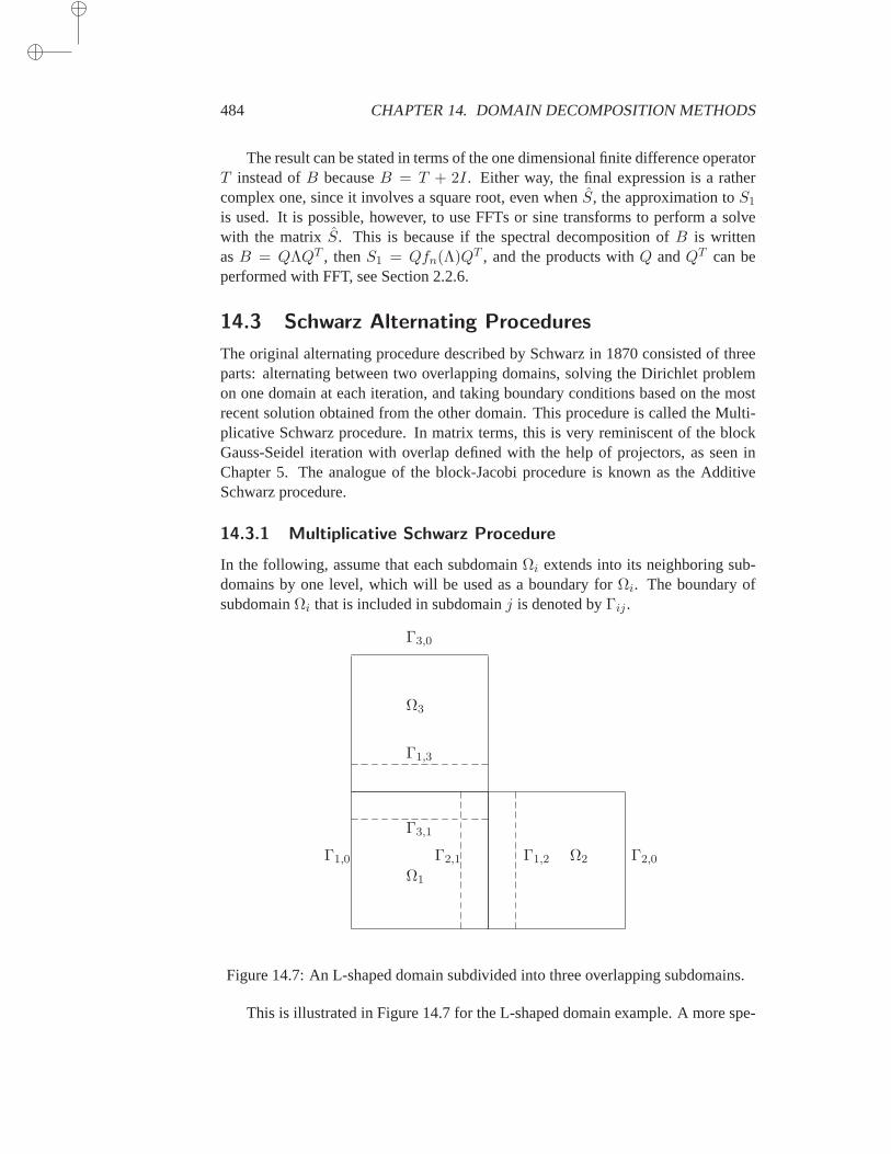
484 CHAPTER 14. DOMAIN DECOMPOSITION METHODS
The result can be stated in terms of the one dimensional finite difference operatorT instead ofB becauseB = T + 2I. Either way, the final expression is a rathercomplex one, since it involves a square root, even whenS, the approximation toS1
is used. It is possible, however, to use FFTs or sine transforms to perform a solvewith the matrix S. This is because if the spectral decomposition ofB is writtenasB = QΛQT , thenS1 = Qfn(Λ)QT , and the products withQ andQT can beperformed with FFT, see Section 2.2.6.
14.3 Schwarz Alternating Procedures
The original alternating procedure described by Schwarz in 1870 consisted of threeparts: alternating between two overlapping domains, solving the Dirichlet problemon one domain at each iteration, and taking boundary conditions based on the mostrecent solution obtained from the other domain. This procedure is called theMulti-plicative Schwarz procedure. In matrix terms, this is very reminiscent of theblockGauss-Seidel iteration with overlap defined with the help of projectors, as seen inChapter 5. The analogue of the block-Jacobi procedure is known as the AdditiveSchwarz procedure.
14.3.1 Multiplicative Schwarz Procedure
In the following, assume that each subdomainΩi extends into its neighboring sub-domains by one level, which will be used as a boundary forΩi. The boundary ofsubdomainΩi that is included in subdomainj is denoted byΓij .
Ω1
Ω3
Ω2
Γ1,3
Γ3,1
Γ2,1 Γ1,2Γ1,0 Γ2,0
Γ3,0
Figure 14.7: An L-shaped domain subdivided into three overlapping subdomains.
This is illustrated in Figure 14.7 for the L-shaped domain example. A more spe-
14.3. SCHWARZ ALTERNATING PROCEDURES 485
cific illustration is in Figure (14.5), where, for example,Γ12 = 29, 30, 31, 32 andΓ31 = 13, 14, 15, 16. Call Γi the boundary ofΩi consisting of its original bound-ary (which consists of theΓi0 pieces in the figure) and theΓij ’s, and denote byuji
the restriction of the solutionu to the boundaryΓji. Then the Schwarz AlternatingProcedure can be described as follows.
ALGORITHM 14.2 SAP
1. Choose an initial guessu to the solution2. Until convergence Do:3. Fori = 1, · · · , s Do:4. Solve∆u = f in Ωi with u = uij in Γij
5. Updateu values onΓji, ∀j6. EndDo7. EndDo
The algorithm sweeps through thes subdomains and solves the original equation ineach of them by using boundary conditions that are updated from the mostrecentvalues ofu. Since each of the subproblems is likely to be solved by some iterativemethod, we can take advantage of a good initial guess. It is natural to take as initialguess for a given subproblem the most recent approximation. Going back to theexpression (14.11) of the local problems, observe that each of the solutions in line 4of the algorithm will be translated into an update of the form
ui := ui + δi,
where the correctionδi solves the system
Aiδi = ri.
Here,ri is the local part of the most recent global residual vectorb − Ax, and theabove system represents the system associated with the problem in line 4 of thealgorithm when a nonzero initial guess is used in some iterative procedure.ThematrixAi has the block structure (14.9). Writing
ui =
(xi
yi
)
, δi =
(δx,i
δy,i
)
, ri =
(rx,i
ry,i
)
,
the correction to the current solution step in the algorithm leads to
(xi
yi
)
:=
(xi
yi
)
+
(Bi Ei
Fi Ci
)−1(rx,i
ry,i
)
. (14.21)
After this step is taken, normally a residual vectorr would have to be computedagain to get the components associated with domaini + 1 and to proceed with asimilar step for the next subdomain. However, only those residual components thathave been affected by the change of the solution need to be updated. Specifically,
486 CHAPTER 14. DOMAIN DECOMPOSITION METHODS
employing the same notation used in equation (14.11), we can simply update theresidualry,j for each subdomainj for which i ∈ Nj as
ry,j := ry,j − Ejiδy,i.
This amounts implicitly to performing Step 5 of the above algorithm. Note that sincethe matrix pattern is assumed to be symmetric, then the set of all indicesj such thati ∈ Nj , i.e.,N∗
i = j |i ∈ Ni, is identical toNi. Now the loop starting in line 3of Algorithm 14.2 and calleddomain sweepcan be restated as follows.
ALGORITHM 14.3 Multiplicative Schwarz Sweep – Matrix Form
1. Fori = 1, · · · , s Do:2. SolveAiδi = ri3. Computexi := xi + δx,i, yi := yi + δy,i, and setri := 04. For eachj ∈ Ni Computery,j := ry,j − Ejiδy,i
5. EndDo
Considering only they iterates, the above iteration would resemble a form of Gauss-Seidel procedure on the Schur complement matrix (14.14). In fact, it is mathemati-cally equivalent, provided a consistent initial guess is taken. This is stated inthe nextresult established by Chan and Goovaerts [73]:
Theorem 14.2 Let the guess
(x(0)i
y(0)i
)
for the Schwarz procedure in each subdomain
be chosen such thatx
(0)i = B−1
i [fi − Eiy(0)i ]. (14.22)
Then they iterates produced by the Algorithm 14.3 are identical to those of a Gauss-Seidel sweep applied to the Schur complement system (14.12).
Proof. We start by showing that with the choice (14.22), they components of theinitial residuals produced by the algorithm are identical to those of the Schurcom-plement system (14.12). Refer to Section 14.2.3 and the relation (14.10) which de-fines theEij ’s from the block structure (14.8) of the global matrix. Observe that
Aijuj =(
0Eijyj
)
and note from (14.11) that for the global system they componentsof the initial residual vectors are
r(0)y,i = gi − Fix
(0)i − Ciy
(0)i −
∑
j∈Ni
Eijy(0)j
= gi − FiB−1[fi − Eiy
(0)i ]− Ciy
(0)i −
∑
j∈Ni
Eijy(0)j
= gi − FiB−1fi − Siy
(0)i −
∑
j∈Ni
Eijy(0)j .
This is precisely the expression of the residual vector associated with the Schur com-plement system (14.12) with the initial guessy(0)
i .
14.3. SCHWARZ ALTERNATING PROCEDURES 487
Now observe that the initial guess has been selected so thatr(0)x,i = 0 for all i.
Because only they components of the residual vector are modified, according to line4 of Algorithm 14.3, this property remains valid throughout the iterative process. Bythe updating equation (14.21) and the relation (14.7), we have
yi := yi + S−1i ry,i,
which is precisely a Gauss-Seidel step associated with the system (14.14).Note thatthe update of the residual vector in the algorithm results in the same update fortheycomponents as in the Gauss-Seidel iteration for (14.14).
It is interesting to interpret Algorithm 14.2, or rather its discrete version, in termsof projectors. For this we follow the model of the overlapping block-Jacobi techniqueseen in the previous chapter. LetSi be an index set
Si = j1, j2, . . . , jni,
where the indicesjk are those associated with theni mesh points of the interior ofthe discrete subdomainΩi. Note that as before, theSi’s form a collection of indexsets such that ⋃
i=1,...,s
Si = 1, . . . , n,
and theSi’s are not necessarily disjoint. LetRi be arestriction operatorfrom Ωto Ωi. By definition,Rix belongs toΩi and keeps only those components of anarbitrary vectorx that are inΩi. It is represented by anni × n matrix of zeros andones. The matricesRi associated with the partitioning of Figure 14.4 are representedin the three diagrams of Figure 14.8, where each square represents a nonzero element(equal to one) and every other element is a zero. These matrices dependon theordering chosen for the local problem. Here, boundary nodes are labeled last, forsimplicity. Observe that each row of eachRi has exactly one nonzero element (equalto one). Boundary points such as the nodes 36 and 37 are representedseveral timesin the matricesR1, R2, andR3 because of the overlapping of the boundary points.Thus, node36 is represented in matricesR1 andR2, while 37 is represented in allthree matrices.
From the linear algebra point of view, the restriction operatorRi is anni × nmatrix formed by the transposes of columnsej of then × n identity matrix, wherej belongs to the index setSi. The transposeRT
i of this matrix is aprolongationoperatorwhich takes a variable fromΩi andextendsit to the equivalent variable inΩ. The matrix
Ai = RiARTi
of dimensionni×ni defines a restriction ofA to Ωi. Now a problem associated withAi can be solved which would update the unknowns in the domainΩi. With thisnotation, the multiplicative Schwarz procedure can be described as follows:

488 CHAPTER 14. DOMAIN DECOMPOSITION METHODS
1. Fori = 1, . . . , s Do2. x := x+RT
i A−1i Ri(b−Ax)
3. EndDo
R1 =
R2 =
R3 =
Figure 14.8: Patterns of the three matricesRi associated with the partitioning ofFigure 14.4.
We change notation and rewrite step 2 as
xnew = x+RTi A
−1i Ri(b−Ax). (14.23)
If the errorsd = x∗ − x are considered wherex∗ is the exact solution, then noticethat b − Ax = A(x∗ − x) and, at each iteration the following equation relates thenew errordnew and the previous errord,
dnew = d−RTi A
−1i RiAd.
Starting from a givenx0 whose error vector isd0 = x∗ − x, each sub-iterationproduces an error vector which satisfies the relation
di = di−1 −RTi A
−1i RiAdi−1,
for i = 1, . . . , s. As a result,
di = (I − Pi)di−1
14.3. SCHWARZ ALTERNATING PROCEDURES 489
in whichPi = RT
i A−1i RiA. (14.24)
Observe that the operatorPi ≡ RTi A
−1i RiA is a projector since
(RTi A
−1i RiA)2 = RT
i A−1i (RiAR
Ti )A−1
i RiA = RTi A
−1i RiA.
Thus, one sweep produces an error which satisfies the relation
ds = (I − Ps)(I − Ps−1) . . . (I − P1)d0. (14.25)
In the following, we use the notation
Qs ≡ (I − Ps)(I − Ps−1) . . . (I − P1). (14.26)
14.3.2 Multiplicative Schwarz Preconditioning
Because of the equivalence of the multiplicative Schwarz procedure anda blockGauss-Seidel iteration, it is possible to recast one Multiplicative Schwarz sweep inthe form of a global fixed-point iteration of the formxnew = Gx + f . Recall thatthis is a fixed-point iteration for solving thepreconditionedsystemM−1Ax = M−1bwhere the preconditioning matrixM and the matrixG are related byG = I−M−1A.To interpret the operation associated withM−1, it is helpful to identify the re-sult of the error vector produced by this iteration with that of (14.25), which isxnew − x∗ = Qs(x− x∗). This comparison yields,
xnew = Qsx+ (I −Qs)x∗,
and therefore,G = Qs f = (I −Qs)x∗.
Hence, the preconditioned matrix isM−1A = I − Qs. This result is restated asfollows.
Proposition 14.3 The multiplicative Schwarz procedure is equivalent to a fixed-point iteration for the “preconditioned” problem
M−1Ax = M−1b,
in which
M−1A = I −Qs (14.27)
M−1b = (I −Qs)x∗ = (I −Qs)A−1b. (14.28)
The transformed right-hand side in the proposition is not known explicitly since itis expressed in terms of the exact solution. However, a procedure can be found tocompute it. In other words, it is possible to operate withM−1 without invokingA−1. Note thatM−1 = (I − Qs)A
−1. As the next lemma indicates,M−1, as wellasM−1A, can be computed recursively.

490 CHAPTER 14. DOMAIN DECOMPOSITION METHODS
Lemma 14.4 Define the matrices
Zi = I −Qi (14.29)
Mi = ZiA−1 (14.30)
Ti = PiA−1 = RT
i A−1i Ri (14.31)
for i = 1, . . . , s. ThenM−1 = Ms, M−1A = Zs, and the matricesZi andMi
satisfy the recurrence relations
Z1 = P1,
Zi = Zi−1 + Pi(I − Zi−1), i = 2, . . . , s (14.32)
and
M1 = T1,
Mi = Mi−1 + Ti(I −AMi−1), i = 2, . . . , s. (14.33)
Proof. It is clear by the definitions (14.29) and (14.30) thatMs = M−1 and thatM1 = T1, Z1 = P1. For the casesi > 1, by definition ofQi andQi−1
Zi = I − (I − Pi)(I − Zi−1) = Pi + Zi−1 − PiZi−1, (14.34)
which gives the relation (14.32). Multiplying (14.34) to the right byA−1 yields,
Mi = Ti +Mi−1 − PiMi−1.
Rewriting the termPi asTiA above yields the desired formula (14.33).
Note that (14.32) yields immediately the important relation
Zi =i∑
j=1
PjQj−1. (14.35)
If the relation (14.33) is multiplied to the right by a vectorv and if the vectorMiv isdenoted byzi, then the following recurrence results.
zi = zi−1 + Ti(v −Azi−1).
Sincezs = (I − Qs)A−1v = M−1v, the end result is thatM−1v can be computed
for an arbitrary vectorv, by the following procedure.
ALGORITHM 14.4 Multiplicative Schwarz Preconditioner
1. Input:v; Output:z = M−1v.2. z := T1v3. Fori = 2, . . . , s Do:4. z := z + Ti(v −Az)5. EndDo
14.3. SCHWARZ ALTERNATING PROCEDURES 491
By a similar argument, a procedure can be found to compute vectors of the formz = M−1Av. In this case, the following algorithm results:
ALGORITHM 14.5 Multiplicative Schwarz Preconditioned Operator
1. Input:v, Output:z = M−1Av.2. z := P1v3. Fori = 2, . . . , s Do4. z := z + Pi(v − z)5. EndDo
In summary, the Multiplicative Schwarz procedure is equivalent to solving the“preconditioned system”
(I −Qs)x = g (14.36)
where the operationz = (I −Qs)v can be computed from Algorithm 14.5 andg =M−1b can be computed from Algorithm 14.4. Now the above procedures can be usedwithin an accelerator such as GMRES. First, to obtain the right-hand sideg of thepreconditioned system (14.36), Algorithm 14.4 must be applied to the originalright-hand sideb. Then GMRES can be applied to (14.36) in which the preconditionedoperationsI −Qs are performed by Algorithm 14.5.
Another important aspect of the Multiplicative Schwarz procedure is that multi-coloring can be exploited in the same way as it is done traditionally for block SOR.Finally, note that symmetry is lost in the preconditioned system but it can be recov-ered by following the sweep 1, 2,. . . , s by a sweep in the other direction, namely,s− 1, s− 2, . . . , 1. This yields a form of the block SSOR algorithm.
14.3.3 Additive Schwarz Procedure
The additive Schwarz procedure is similar to a block-Jacobi iteration and consistsof updating all the new (block) components from the same residual. Thus, itdiffersfrom the multiplicative procedure only because the components in each subdomainare not updated until a whole cycle of updates through all domains are completed.The basic Additive Schwarz iteration would therefore be as follows:
1. Fori = 1, . . . , s Do2. Computeδi = RT
i A−1i Ri(b−Ax)
3. EndDo4. xnew = x+
∑si=1 δi
The new approximation (obtained after a cycle of thes substeps in the abovealgorithm are applied) is
xnew = x+s∑
i=1
RTi A
−1i Ri(b−Ax).
492 CHAPTER 14. DOMAIN DECOMPOSITION METHODS
Each instance of the loop redefines different components of the new approximationand there is no data dependency between the subproblems involved in the loop.
The preconditioning matrix is rather simple to obtain for the additive Schwarzprocedure. Using the matrix notation defined in the previous section, notice that thenew iterate satisfies the relation
xnew = x+s∑
i=1
Ti(b−Ax) =
(
I −s∑
i=1
Pi
)
x+s∑
i=1
Tib.
Thus, using the same analogy as in the previous section, this iteration corresponds toa fixed-point iterationxnew = Gx+ f with
G = I −s∑
i=1
Pi, f =s∑
i=1
Tib.
With the relationG = I −M−1A, betweenG and the preconditioning matrixM ,the result is that
M−1A =s∑
i=1
Pi,
and
M−1 =s∑
i=1
PiA−1 =
s∑
i=1
Ti.
Now the procedure for applying the preconditioned operatorM−1 becomes clear.
ALGORITHM 14.6 Additive Schwarz Preconditioner
1. Input:v; Output:z = M−1v.2. Fori = 1, . . . , s Do:3. Computezi := Tiv4. EndDo5. Computez := z1 + z2 . . .+ zs.
Note that the do loop can be performed in parallel. Step 5 sums up the vectorsziin each domain to obtain a global vectorz. In the nonoverlapping case, this step isparallel and consists of just forming these different components since the addition istrivial. In the presence of overlap, the situation is similar except that the overlappingcomponents are added up from the different results obtained in each subdomain.
The procedure for computingM−1Av is identical to the one above except thatTi in line 3 is replaced byPi.
14.3.4 Convergence
Throughout this section, it is assumed thatA is Symmetric Positive Definite. TheprojectorsPi defined by (14.24) play an important role in the convergence theory ofboth additive and multiplicative Schwarz. A crucial observation here is thatthese

14.3. SCHWARZ ALTERNATING PROCEDURES 493
projectors are orthogonal with respect to theA-inner product. Indeed, it is sufficientto show thatPi is self-adjoint with respect to theA-inner product,
(Pix, y)A = (ARTi A
−1i RiAx, y) = (Ax,RT
i A−1i RiAy) = (x, Piy)A.
Consider the operator,
AJ =s∑
i=1
Pi. (14.37)
Since eachPj is self-adjoint with respect to theA-inner product, i.e.,A-self-adjoint,their sumAJ is alsoA-self-adjoint. Therefore, it will have real eigenvalues. An im-mediate consequence of the fact that thePi’s are projectors is stated in the followingtheorem.
Theorem 14.5 The largest eigenvalue ofAJ is such that
λmax(AJ) ≤ s,wheres is the number of subdomains.
Proof. For any matrix norm,λmax(AJ) ≤ ‖AJ‖. In particular, if theA-norm isused, we have
λmax(AJ) ≤s∑
i=1
‖Pi‖A.
Each of theA-norms ofPi is equal to one sincePi is anA-orthogonal projector. Thisproves the desired result.
This result can be improved substantially by observing that the projectors can begrouped in sets that have disjoint ranges. Graph coloring techniques seen in Chap-ter 3 can be used to obtain such colorings of the subdomains. Assume thatc setsof indicesΘi, i = 1, . . . , c are such that all the subdomainsΩj for j ∈ Θi have nointersection with one another. Then,
PΘi=∑
j ∈ Θi
Pj (14.38)
is again an orthogonal projector.This shows that the result of the previous theorem can be improved triviallyinto
the following.
Theorem 14.6 Suppose that the subdomains can be colored in such a way that twosubdomains with the same color have no common nodes. Then, the largest eigenvalueofAJ is such that
λmax(AJ) ≤ c,wherec is the number of colors.
In order to estimate the lowest eigenvalue of the preconditioned matrix, an assump-tion must be made regarding the decomposition of an arbitrary vectorx into compo-nents ofΩi.

494 CHAPTER 14. DOMAIN DECOMPOSITION METHODS
Assumption 1. There exists a constantK0 such that the inequality
s∑
i=1
(Aui, ui) ≤ K0(Au, u),
is satisfied by the representation ofu ∈ Ω as the sum
u =
s∑
i=1
ui, ui ∈ Ωi.
The following theorem has been proved by several authors in slightly different formsand contexts.
Theorem 14.7 If Assumption 1 holds, then
λmin(AJ) ≥ 1
K0.
Proof. Unless otherwise stated, all summations in this proof are from1 to s. Startwith an arbitraryu decomposed asu =
∑ui and write
(u, u)A =∑
(ui, u)A =∑
(Piui, u)A =∑
(ui, Piu)A.
The last equality is due to the fact thatPi is anA-orthogonal projector ontoΩi andit is therefore self-adjoint. Now, using Cauchy-Schwarz inequality, we get
(u, u)A =∑
(ui, Piu)A ≤(∑
(ui, ui)A
)1/2 (∑
(Piu, Piu)A
)1/2.
By Assumption 1, this leads to
‖u‖2A ≤ K1/20 ‖u‖A
(∑
(Piu, Piu)A
)1/2,
which, after squaring, yields
‖u‖2A ≤ K0
∑
(Piu, Piu)A.
Finally, observe that since eachPi is anA-orthogonal projector, we have
∑
(Piu, Piu)A =∑
(Piu, u)A =(∑
Piu, u)
A.
Therefore, for anyu, the inequality
(AJu, u)A ≥1
K0(u, u)A
holds, which yields the desired upper bound by the min-max theorem.
14.3. SCHWARZ ALTERNATING PROCEDURES 495
Note that the proof uses the following form of the Cauchy-Schwarz inequality:
p∑
i=1
(xi, yi) ≤(
p∑
i=1
(xi, xi)
)1/2( p∑
i=1
(yi, yi)
)1/2
.
See Exercise 1 for a proof of this variation.We now turn to the analysis of the Multiplicative Schwarz procedure. We start
by recalling that the error after each outer iteration (sweep) is given by
d = Qsd0.
We wish to find an upper bound for‖Qs‖A. First note that (14.32) in Lemma 14.4results in
Qi = Qi−1 − PiQi−1,
from which we get, using theA-orthogonality ofPi,
‖Qiv‖2A = ‖Qi−1v‖2A − ‖PiQi−1v‖2A.
The above equality is valid fori = 1, providedQ0 ≡ I. Summing these equalitiesfrom i = 1 to s gives the result,
‖Qsv‖2A = ‖v‖2A −s∑
i=1
‖PiQi−1v‖2A. (14.39)
This indicates that theA-norm of the error will not increase at each substep of thesweep.
Now a second assumption must be made to prove the next lemma.
Assumption 2. For any subsetS of 1, 2, . . . , s2 andui, vj ∈ Ω, the followinginequality holds:
∑
(i,j) ∈ S
(Piui, Pjvj)A ≤ K1
(s∑
i=1
‖Piui‖2A
)1/2
s∑
j=1
‖Pjvj‖2A
1/2
. (14.40)
Lemma 14.8 If Assumptions 1 and 2 are satisfied, then the following is true,
s∑
i=1
‖Piv‖2A ≤ (1 +K1)2
s∑
i=1
‖PiQi−1v‖2A. (14.41)
Proof. Begin with the relation which follows from the fact thatPi is anA-orthogonalprojector,
(Piv, Piv)A = (Piv, PiQi−1v)A + (Piv, (I −Qi−1)v)A,
496 CHAPTER 14. DOMAIN DECOMPOSITION METHODS
which yields, with the help of (14.35),
s∑
i=1
‖Piv‖2A =s∑
i=1
(Piv, PiQi−1v)A +s∑
i=1
i−1∑
j=1
(Piv, PjQj−1v)A. (14.42)
For the first term of the right-hand side, use the Cauchy-Schwarz inequality to obtain
s∑
i=1
(Piv, PiQi−1v)A ≤(
s∑
i=1
‖Piv‖2A
)1/2( s∑
i=1
‖PiQi−1v‖2A
)1/2
.
For the second term of the right-hand side of (14.42), use the assumption (14.40) toget
s∑
i=1
i−1∑
j=1
(Piv, PjQj−1v)A ≤ K1
(s∑
i=1
‖Piv‖2A)
)1/2
s∑
j=1
‖PjQj−1v‖2A)
1/2
.
Adding these two inequalities, squaring the result, and using (14.42) leads totheinequality (14.41).
From (14.39), it can be deduced that if Assumption 2 holds, then,
‖Qsv‖2A ≤ ‖v‖2A −1
(1 +K1)2
s∑
i=1
‖Piv‖2A. (14.43)
Assumption 1 can now be exploited to derive a lower bound on∑s
i=1 ‖Piv‖2A. Thiswill yield the following theorem.
Theorem 14.9 Assume that Assumptions 1 and 2 hold. Then,
‖Qs‖A ≤[
1− 1
K0(1 +K1)2
]1/2
. (14.44)
Proof. Using the notation of Section 14.3.3, the relation‖Piv‖2A = (Piv, v)A yields
s∑
i=1
‖Piv‖2A =
(s∑
i=1
Piv, v
)
A
= (AJv, v)A.
According to Theorem 14.7,λmin(AJ) ≥ 1K0
, which implies(AJv, v)A ≥ (v, v)A/K0.Thus,
s∑
i=1
‖Piv‖2A ≥(v, v)A
K0,
which upon substitution into (14.43) gives the inequality
‖Qsv‖2A‖v‖2A
≤ 1− 1
K0(1 +K1)2.
The result follows by taking the maximum over all vectorsv.
14.4. SCHUR COMPLEMENT APPROACHES 497
This result provides information on the speed of convergence of the multiplica-tive Schwarz procedure by making two key assumptions. These assumptions are notverifiable from linear algebra arguments alone. In other words, given alinear sys-tem, it is unlikely that one can establish that these assumptions are satisfied. How-ever, they are satisfied for equations originating from finite element discretizationof elliptic Partial Differential Equations. For details, refer to Dryja and Widlund[102, 103, 104] and Xu [320].
14.4 Schur Complement Approaches
Schur complement methods are based on solving the reduced system (14.4)by somepreconditioned Krylov subspace method. Procedures of this type involvethree steps.
1. Get the right-hand sideg′ = g − FB−1f .2. Solve the reduced systemSy = g′ via an iterative method.3. Back-substitute, i.e., computex via (14.3).
The different methods relate to the way in which step 2 is performed. Firstobserve that the matrixS need not be formed explicitlyin order to solve the reducedsystem by an iterative method. For example, if a Krylov subspace method withoutpreconditioning is used, then the only operations that are required with the matrixS are matrix-by-vector operationsw = Sv. Such operations can be performed asfollows.
1. Computev′ = Ev,2. SolveBz = v′
3. Computew = Cv − Fz.
The above procedure involves only matrix-by-vector multiplications and one lin-ear system solution withB. Recall that a linear system involvingB translates intos-independent linear systems. Also note that the linear systems withB must besolved exactly, either by a direct solution technique or by an iterative technique witha high level of accuracy.
While matrix-by-vector multiplications withS cause little difficulty, it is muchharder to precondition the matrixS, since this full matrix is often not available ex-plicitly. There have been a number of methods, derived mostly using argumentsfrom Partial Differential Equations to precondition the Schur complement. Here, weconsider only those preconditioners that are derived from a linear algebra viewpoint.
14.4.1 Induced Preconditioners
One of the easiest ways to derive an approximation toS is to exploit Proposition 14.1and the intimate relation between the Schur complement and Gaussian elimination.
498 CHAPTER 14. DOMAIN DECOMPOSITION METHODS
This proposition tells us that a preconditioning operatorM to S can be defined fromthe (approximate) solution obtained withA. To precondition a given vectorv, i.e.,to computew = M−1v, whereM is the desired preconditioner toS, first solve thesystem
A
(xy
)
=
(0v
)
, (14.45)
then takew = y. Use any approximate solution technique to solve the above system.Let MA be any preconditioner forA. Using the notation defined earlier, letRy
represent the restriction operator on the interface variables, as defined in Proposition14.1. Then the preconditioning operation forS which is induced fromMA is definedby
M−1S v = RyM
−1A
(0v
)
= RyM−1A RT
y v.
Observe that whenMA is an exact preconditioner, i.e., whenMA = A, then accord-ing to Proposition 14.1,MS is also an exact preconditioner, i.e.,MS = S. Thisinduced preconditioner can be expressed as
MS =(RyM
−1A RT
y
)−1. (14.46)
It may be argued that this uses a preconditioner related to the original problem tobe solved in the first place. However, even though the preconditioning onS may bedefined from a preconditioning ofA, the linear system is being solved for the inter-face variables. That is typically much smaller than the original linear system. Forexample, GMRES can be used with a much larger dimension of the Krylov subspacesince the Arnoldi vectors to keep in memory are much smaller. Also note that froma Partial Differential Equations viewpoint, systems of the form (14.45) correspondto the Laplace equation, the solutions of which are “Harmonic” functions. There arefast techniques which provide the solution of such equations inexpensively.
In the case whereMA is an ILU factorization ofA, MS can be expressed in anexplicit form in terms of the entries of the factors ofMA. This defines a precondi-tioner toS that is induced canonically from an incomplete LU factorization ofA.Assume that the preconditionerMA is in a factored formMA = LAUA, where
LA =
(LB 0FU−1
B LS
)
UA =
(UB L−1
B E0 US
)
.
Then, the inverse ofMA will have the following structure:
M−1A = U−1
A L−1A
=
(⋆ ⋆0 U−1
S
)(⋆ 0⋆ L−1
S
)
=
(⋆ ⋆⋆ U−1
S L−1S
)
where a star denotes a matrix whose actual expression is unimportant. Recall that bydefinition,
Ry = ( 0 I ) ,
14.4. SCHUR COMPLEMENT APPROACHES 499
where this partitioning conforms to the above ones. This means that
RyM−1A RT
y = U−1S L−1
S
and, therefore, according to (14.46),MS = LSUS . This result is stated in the fol-lowing proposition.
Proposition 14.10 Let MA = LAUA be an ILU preconditioner forA. Then thepreconditionerMS for S induced byMA, as defined by (14.46), is given by
MS = LSUS , with LS = RyLARTy , US = RyUAR
Ty .
In words, the proposition states that the L and U factors forMS are the(2, 2) blocksof the L and U factors of the ILU factorization ofA. An important consequence ofthe above idea is that the parallel Gaussian elimination can be exploited for derivingan ILU preconditioner forS by using a general purpose ILU factorization. In fact,theL andU factors ofMA have the following structure:
A = LAUA −R with,
LA =
L1
L2.. .
Ls
F1U−11 F2U
−12 · · · FsU
−1s L
UA =
U1 L−11 E1
U2 L−12 E2
.. ....
Us L−1s Es
U
.
EachLi, Ui pair is an incomplete LU factorization of the localBi matrix. These ILUfactorizations can be computed independently. Similarly, the matricesL−1
i Ei andFiU
−1i can also be computed independently once the LU factors are obtained. Then
each of the matricesSi = Ci − FiU
−1i L−1
i Ei,
which are the approximate local Schur complements, is obtained. Note that since anincomplete LU factorization is being performed, some drop strategy is applied totheelements inSi. LetTi be the matrix obtained after this is done,
Ti = Si −Ri.
Then a final stage would be to compute the ILU factorization of the matrix (14.14)where eachSi is replaced byTi.
500 CHAPTER 14. DOMAIN DECOMPOSITION METHODS
14.4.2 Probing
To derive preconditioners for the Schur complement, another general purpose tech-nique exploits ideas used in approximating sparse Jacobians when solving nonlinearequations. In general,S is a dense matrix. However, it can be observed, and thereare physical justifications for model problems,
that its entries decay away from the main diagonal. Assume thatS is nearlytridiagonal, i.e., neglect all diagonals apart from the main diagonal and the two codi-agonals, and write the corresponding tridiagonal approximation toS as
T =
a1 b2c2 a2 b3
. . . . . . . ..cm−1 am−1 bm
cm am
.
Then, it is easy to recoverT by applying it to three well-chosen vectors. Considerthe three vectors
w1 = (1, 0, 0, 1, 0, 0, 1, 0, 0, . . . , )T ,
w2 = (0, 1, 0, 0, 1, 0, 0, 1, 0, . . . , )T ,
w3 = (0, 0, 1, 0, 0, 1, 0, 0, 1, . . . , )T .
Then we have
Tw1 = (a1, c2, b4, a4, c5, . . . , b3i+1, a3i+1, c3i+2, . . .)T ,
Tw2 = (b2, a2, c3, b5, a5, c6, . . . , b3i+2, a3i+2, c3i+3, . . .)T ,
Tw3 = (b3, a3, c4, b6, a6, c7, . . . , b3i, a3i, c3i+1, . . .)T .
This shows that all the coefficients of the matrixT are indeed all represented in theabove three vectors. The first vector contains the nonzero elements of the columns1, 4, 7, . . ., 3i + 1, . . ., in succession written as a long vector. Similarly,Tw2
contains the columns2, 5, 8, . . ., andTw3 contains the columns3, 6, 9, . . .. We caneasily computeSwi, i = 1, 3 and obtain a resulting approximationT which can beused as a preconditioner toS. The idea can be extended to compute any bandedapproximation toS. For details and analysis see [74].
14.4.3 Preconditioning Vertex-Based Schur Complements
We now discuss some issues related to the preconditioning of a linear system withthe matrix coefficient of (14.14) associated with a vertex-based partitioning. As wasmentioned before, this structure is helpful in the direct solution context because itallows the Schur complement to be formed by local pieces. Since incomplete LUfactorizations will utilize the same structure, this can be exploited as well.
Note that multicolor SOR or SSOR can also be exploited and that graph color-ing can be used to color the interface valuesyi in such a way that no two adjacent

14.5. FULL MATRIX METHODS 501
interface variables will have the same color. In fact, this can be achieved by coloringthe domains. In the course of a multicolor block-SOR iteration, a linear system mustbe solved with the diagonal blocksSi. For this purpose, it is helpful to interpret theSchur complement. CallP the canonical injection matrix from the local interfacepoints to the local nodes. Ifni points are local and ifmi is the number of the localinterface points, thenP is anni×mi matrix whose columns are the lastmi columnsof theni × ni identity matrix. Then it is easy to see that
Si = (P TA−1loc,iP )−1. (14.47)
If Aloc,i = LU is the LU factorization ofAloc,i then it can be verified that
S−1i = P TU−1L−1P = P TU−1PP TL−1P, (14.48)
which indicates that in order to operate withP TL−1P , the lastmi × mi principalsubmatrix ofL must be used. The same is true forP TU−1P which requires only aback-solve with the lastmi ×mi principal submatrix ofU . Therefore, only the LUfactorization ofAloc,i is needed to solve a system with the matrixSi. Interestingly,approximate solution methods associated with incomplete factorizations ofAloc,i canbe exploited.
14.5 Full Matrix Methods
We call any technique that iterates on the original system (14.2) afull matrix method.In the same way that preconditioners were derived from the LU factorization of Afor the Schur complement, preconditioners forA can be derived from approximatinginterface values.
Before starting with preconditioning techniques, we establish a few simple rela-tions between iterations involvingA andS.
Proposition 14.11 Let
LA =
(I O
FB−1 I
)
, UA =
(B EO I
)
(14.49)
and assume that a Krylov subspace method is applied to the original system(14.1)with left preconditioningLA and right preconditioningUA, and with an initial guessof the form (
x0
y0
)
=
(B−1(f − Ey0)
y0
)
. (14.50)
Then this preconditioned Krylov iteration will produce iterates of the form(xm
ym
)
=
(B−1(f − Eym)
ym
)
(14.51)
in which the sequenceym is the result of the same Krylov subspace method appliedwithout preconditioning to the reduced linear systemSy = g′ with g′ = g−FB−1fstarting with the vectory0.
502 CHAPTER 14. DOMAIN DECOMPOSITION METHODS
Proof. The proof is a consequence of the factorization(B EF C
)
=
(I O
FB−1 I
)(I OO S
)(B EO I
)
. (14.52)
Applying an iterative method (e.g., GMRES) on the original system, preconditionedfrom the left byLA and from the right byUA, is equivalent to applying this iterativemethod to
L−1A AU−1
A =
(I OO S
)
≡ A′. (14.53)
The initial residual for the preconditioned system is
L−1A
(f
g
)
− (L−1A AU−1
A )UA
(x0
y0
)
=
(I O
−FB−1 I
)((f
g
)
−(
fFB−1(f − Ey0) + Cy0
))
=
(0
g′ − Sy0
)
≡(
0r0
)
.
As a result, the Krylov vectors obtained from the preconditioned linear system asso-ciated with the matrixA′ have the form
(0
r0
)
,
(0
Sr0
)
· · · ,(
0
Sm−1r0
)
(14.54)
and the associated approximate solution will be of the form(xm
ym
)
=
(x0
y0
)
+
(B−1 −B−1EO I
)(0
∑m−1i=0 αiS
ir0
)
=
(B−1(f − Ey0)−B−1E(ym − y0)
ym
)
=
(B−1(f − Eym)
ym
)
.
Finally, the scalarsαi that express the approximate solution in the Krylov basis areobtained implicitly via inner products of vectors among the vector sequence (14.54).These inner products are identical to those of the sequencer0, Sr0, · · · , Sm−1r0.Therefore, these coefficients will achieve the same result as the same Krylov methodapplied to the reduced systemSy = g′, if the initial guess gives the residual guessr0.
A version of this proposition should allowS to be preconditioned. The followingresult is an immediate extension that achieves this goal.
Proposition 14.12 Let S = LSUS − R be an approximate factorization ofS anddefine
LA =
(I O
FB−1 LS
)
, UA =
(B EO US
)
. (14.55)
14.5. FULL MATRIX METHODS 503
Assume that a Krylov subspace method is applied to the original system (14.1) withleft preconditioningLA and right preconditioningUA, and with an initial guess ofthe form (
x0
y0
)
=
(B−1(f − Ey0)
y0
)
. (14.56)
Then this preconditioned Krylov iteration will produce iterates of the form(xm
ym
)
=
(B−1(f − Eym)
ym
)
. (14.57)
Moreover, the sequenceym is the result of the same Krylov subspace method appliedto the reduced linear systemSy = g − FB−1f , left preconditioned withLS , rightpreconditioned withUS , and starting with the vectory0.
Proof. The proof starts with the equality(B EF C
)
=
(I O
FB−1 LS
)(I OO L−1
S SU−1S
)(B EO US
)
. (14.58)
The rest of the proof is similar to that of the previous result and is omitted.
Also there are two other versions in whichS is allowed to be preconditionedfrom the left or from the right. Thus, ifMS is a certain preconditioner forS, use thefollowing factorizations
(B EF C
)
=
(I O
FB−1 MS
)(I OO M−1
S S
)(B EO I
)
(14.59)
=
(I O
FB−1 I
)(I OO SM−1
S
)(B EO MS
)
, (14.60)
to derive the appropriate left or right preconditioners. Observe that when the precon-ditionerMS to S is exact, i.e., whenM = S, then the block preconditionerLA, UA
toA induced fromMS is also exact.Although the previous results indicate that a Preconditioned Schur Complement
iteration is mathematically equivalent to a certain preconditioned full matrix method,there are some practical benefits in iterating with the nonreduced system. Themainbenefit involves the requirement in the Schur Complement techniques to computeSxexactly at each Krylov subspace iteration. Indeed, the matrixS represents the coeffi-cient matrix of the linear system, and inaccuracies in the matrix-by-vector operationmay result in loss of convergence. In the full matrix techniques, the operation Sx isnever needed explicitly. In addition, this opens up the possibility of preconditioningthe original matrix with approximate solves with the matrixB in the preconditioningoperationLA andUA.
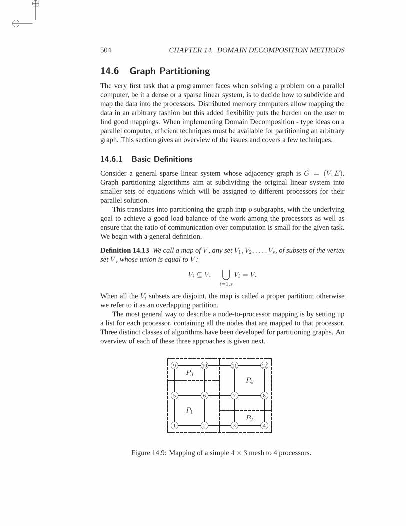
504 CHAPTER 14. DOMAIN DECOMPOSITION METHODS
14.6 Graph Partitioning
The very first task that a programmer faces when solving a problem on a parallelcomputer, be it a dense or a sparse linear system, is to decide how to subdivide andmap the data into the processors. Distributed memory computers allow mapping thedata in an arbitrary fashion but this added flexibility puts the burden on the user tofind good mappings. When implementing Domain Decomposition - type ideas on aparallel computer, efficient techniques must be available for partitioning anarbitrarygraph. This section gives an overview of the issues and covers a few techniques.
14.6.1 Basic Definitions
Consider a general sparse linear system whose adjacency graph isG = (V,E).Graph partitioning algorithms aim at subdividing the original linear system intosmaller sets of equations which will be assigned to different processors for theirparallel solution.
This translates into partitioning the graph intpp subgraphs, with the underlyinggoal to achieve a good load balance of the work among the processors aswell asensure that the ratio of communication over computation is small for the given task.We begin with a general definition.
Definition 14.13 We call a map ofV , any setV1, V2, . . . , Vs, of subsets of the vertexsetV , whose union is equal toV :
Vi ⊆ V,⋃
i=1,s
Vi = V.
When all theVi subsets are disjoint, the map is called a proper partition; otherwisewe refer to it as an overlapping partition.
The most general way to describe a node-to-processor mapping is by setting upa list for each processor, containing all the nodes that are mapped to thatprocessor.Three distinct classes of algorithms have been developed for partitioning graphs. Anoverview of each of these three approaches is given next.
1 2 3 4
5 6 7 8
9 10 11 12
P1
P2
P3
P4
Figure 14.9: Mapping of a simple4× 3 mesh to 4 processors.
14.6. GRAPH PARTITIONING 505
14.6.2 Geometric Approach
The geometric approach works on the physical mesh and requires the coordinates ofthe mesh points. In the simplest case, for a 2-dimensional rectangular grid,stripes inthe horizontal and vertical direction can be defined to get square subregions whichhave roughly the same number of points. Other techniques utilize notions of momentof inertia to divide the region recursively into two roughly equal-sized subregions.
Next is a brief description of a technique based on work by Miller, Teng, Thur-ston, and Vavasis [211]. This technique finds good separators for a mesh using pro-jections into a higher space. Given a mesh inR
d, the method projects the mesh pointsinto a unit sphere centered at the origin inR
d+1. Stereographic projection is used: Aline is drawn from a given pointp in the plane to the North Pole(0, . . . , 0, 1) and thestereographic projection ofp is the point where this line intersects the sphere. In thenext step, acenterpointof the projected points is found. A centerpointc of a discretesetS is defined as a point where every hyperplane passing throughc will divide Sapproximately evenly.
Once the centerpoint is found, the points of the sphere are rotated so thatthecenterpoint is aligned with the North Pole, i.e., so that coordinates ofc are trans-formed into(0, . . . , 0, r). The points are further transformed by dilating them so thatthe centerpoint becomes the origin. Through all these transformations, thepoint cremains a centerpoint. Therefore, if any hyperplane is taken that passes through thecenterpoint which is now the origin, it should cut the sphere into two roughlyequal-sized subsets. Any hyperplane passing through the origin will intersect the spherealong a large circleC. Transforming this circle back into the original space will givea desired separator. Notice that there is an infinity of circles to choose from.
One of the main ingredients in the above algorithm is a heuristic for findingcenterpoints inRd space (actually,Rd+1 in the algorithm). The heuristic that is usedrepeatedly replaces randomly chosen sets ofd+ 2 points by their centerpoint, whichare easy to find in this case. There are a number of interesting results that analyzethe quality of geometric graph partitionings based on separators. With some minimalassumptions on the meshes, it is possible to show that there exist “good” separators.In addition, the algorithm discussed above constructs such separators.We start withtwo definitions.
Definition 14.14 A k-ply neighborhood system inRd is a set ofn closed disksDi,i = 1, . . . , n in R
d such that no point inRd is (strictly) interior to more thank disks.
Definition 14.15 Letα ≥ 1 and letD1, . . . , Dn be ak-ply neighborhood system inR
d. The(α, k)-overlap graph for the neighborhood system is the graph with vertexsetV = 1, 2, . . . , n and edge set, the subset ofV × V defined by
(i, j) : (Di ∩ (α.Dj) 6= φ) and(Dj ∩ (α.Di) 6= φ).
A mesh inRd is associated with an overlap graph by assigning the coordinate of the
centerci of disk i to each nodei of the graph. Overlap graphs model computationalmeshes ind dimensions. Indeed, every mesh with boundedaspect ratioelements
506 CHAPTER 14. DOMAIN DECOMPOSITION METHODS
(ratio of largest to smallest edge length of each element) is contained in an overlapgraph. In addition, any planar graph is an overlap graph. The main result regardingseparators of overlap graphs is the following theorem [211].
Theorem 14.16LetG be ann-vertex(α, k) overlap graph ind dimensions. Thenthe vertices ofG can be partitioned into three setsA,B, andC such that:
1. No edge joinsA andB.
2. A andB each have at mostn(d+ 1)/(d+ 2) vertices.
3. C has onlyO(α k1/dn(d−1)/d) vertices.
Thus, ford = 2, the theorem states that it is possible to partition the graph into twosubgraphsA andB, with a separatorC, such that the number of nodes for each ofAandB does not exceed34n vertices in the worst case and such that the separator hasa number of nodes of the orderO(α k1/2n1/2).
14.6.3 Spectral Techniques
Spectral bisectionrefers to a technique which exploits some known properties of theeigenvectors of theLaplacean of a graph. Given an adjacency graphG = (V,E),we associate to it a Laplacian matrixL which is a sparse matrix having the sameadjacency graphG and defined as follows:
lij =
−1 if(vi, vj) ∈ E and i 6= jdeg(i) if i = j0 otherwise.
These matrices have some interesting fundamental properties. When the graph isundirectedL is symmetric. It can be shown to be alsonegative semi definite(seeExercise 11). Zero is an eigenvalue and it is the smallest one. An eigenvector as-sociated with this eigenvalue is any constant vector, and this eigenvector bears littleinterest. The second smallest eigenvector, called theFiedler vector, has the usefulproperty that the signs of its components divide the domain into roughly two equalsubdomains.
The Recursive Spectral Bisection (RSB) algorithm consists of sorting thecom-ponents of the Fiedler vector and assigning the first half of the sorted vertices tothe first subdomain and the second half to the second subdomain. The two subdo-mains are then partitioned in two recursively, until a desirable number of domains isreached.
ALGORITHM 14.7 RSB (Recursive Spectral Bisection)
1. Compute the Fiedler vectorf of the graphG.2. Sort the components off , e.g., increasingly.3. Assign first⌊n/2⌋ nodes toV1, and the rest toV2 .4. Apply RSB recursively toV1, V2, until the desired number of partitions5. is reached.
14.6. GRAPH PARTITIONING 507
The main theoretical property that is exploited here is that the differences be-tween the components of the Fiedler vector represent some sort of distance betweenthe corresponding nodes. Thus, if these components are sorted they would be effec-tively grouping the associated node by preserving nearness. Anotherinteresting factis that the algorithm will also tend to minimize the numbernc of edge-cuts, i.e., thenumber of edges(vi, vj) such thatvi ∈ V1 andvj ∈ V2. Assume thatV1 andV2
are of equal size and define apartition vectordefinep whosei-th component is+1if vi ∈ V1, and−1 if vi ∈ V2. By the assumptions the sum of allpi’s is zero. Thennotice that
(Lp, p) = 4nc, (p, e) = 0.
Ideally, the objective function(Lp, p) should be minimized subject to the constraint(p, e) = 0. Herep is a vector of signs. If, instead, the objective function(Lx, x)/(x, x)were minimized forx real, subject to(x, e) = 0, the solution would be the Fiedlervector, sincee is the eigenvector associated with the eigenvalue zero. The Fiedlervector can be computed by the Lanczos algorithm or any other method efficient forlarge sparse matrices. Recursive Specrtal Bisection gives excellent partitionings. Onthe other hand, it is rather unattractive because it requires computing an eigenvector.
14.6.4 Graph Theory Techniques
A number of other techniques exist which, like spectral techniques, are also basedon the adjacency graph only. The simplest idea is one that is borrowed from thetechnique ofnested dissectionin the context of direct sparse solution methods, seeSections 3.6.2 and 3.3.3. An initial node is given which constitutes the level zero.Then, the method recursively traverses thek-th level (k ≥ 1), which consists of theneighbors of all the elements that constitute levelk−1. A simple idea for partitioningthe graph in two traverses enough levels to visit about half of all the nodes. Thevisited nodes will be assigned to one subdomain and the others will constitute thesecond subdomain. The process can then be repeated recursively oneach of thesubdomains.
A key ingredient for this technique to be successful is to determine a good initialnode from which to start the traversal. Often, a heuristic is used for this purpose.Recall thatd(x, y) is the distance between verticesx andy in the graph, i.e., thelength of the shortest path betweenx andy.
If the diameter of a graph is defined as
δ(G) = maxd(x, y) | x ∈ V, y ∈ V
then, ideally, one of two nodes in a pair(x, y) that achieves the diameter can be usedas a starting node. Theseperipheral nodes, are expensive to determine. Instead, apseudo-peripheralnode, as defined through the following procedure, is often em-ployed [144]
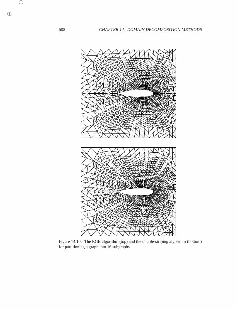
508 CHAPTER 14. DOMAIN DECOMPOSITION METHODS
Figure 14.10: The RGB algorithm (top) and the double-striping algorithm (bottom)for partitioning a graph into 16 subgraphs.
14.6. GRAPH PARTITIONING 509
ALGORITHM 14.8 Pseudo-Peripheral Node
1. Select an initial nodex. Setδ = 0.2. Do a level set traversal fromx3. Select a nodey in the last level set, with minimum degree4. If d(x, y) > δ then5. Setx := y andδ := d(x, y)6. GoTo 27. Else Stop:x is a pseudo-peripheral node.8. EndIf
The distanced(x, y) in line 5 is the number of levels in the level set traversal neededin Step 2. The algorithm traverses the graph from a node of the last level intheprevious traversal, until the number of levels stabilizes. It is easy to see that thealgorithm does indeed stop after a finite number of steps, typically small.
A first heuristic approach based on level set traversals is the recursive dissectionprocedure mentioned above and described next.
ALGORITHM 14.9 Recursive Graph Bisection
1. SetG∗ := G, S := G, ndom := 12. Whilendom < s Do:3. Select inS the subgraphG∗ with largest size.4. Find a pseudo-peripheral nodep in G∗ and5. Do a level set traversal fromp. Let lev := number of levels.6. LetG1 the subgraph ofG∗ consisting of the firstlev/27. levels, andG2 the subgraph containing the rest ofG∗.8. RemoveG∗ from S and addG1 andG2 to it9. ndom := ndom + 1
10. EndWhile
The cost of this algorithm is rather small. Each traversal of a graphG = (V,E) costsaround|E|, where|E| is the number of edges (assuming that|V | = O(|E|)). Sincethere ares traversals of graphs whose size decreases by 2 at each step, it is clear thatthe cost isO(|E|), the order of edges in the original graph. As can be expected, theresults of such an algorithm are not always good. Typically, two qualities that aremeasured are the sizes of the domains as well as the number of edge-cuts.
Ideally, the domains should be equal. In addition, since the values at the interfacepoints should be exchanged with those of neighboring processors, theirtotal number,as determined by the number of edge-cuts, should be as small as possible. The firstmeasure can be easily controlled in a recursive Graph Bisection Algorithm —forexample, by using variants in which the number of nodes is forced to be exactly halfthat of the original subdomain. The second measure is more difficult to control.
As an example, the top part of Figure 14.10 shows the result of the RGB algo-rithm on a sample finite-element mesh. Thus, the top part of Figure 14.10 shows theresult of the RGB algorithm on a sample finite-element mesh. This is a vertex-basedpartitioning. The dashed lines represent the edge-cuts.
510 CHAPTER 14. DOMAIN DECOMPOSITION METHODS
An approach that is competitive with the one described above is that ofdou-ble striping. This method uses two parametersp1, p2 such thatp1p2 = s. Theoriginal graph is first partitioned intop1 large partitions, using one-way partition-ing, then each of these partitions is subdivided intop2 partitions similarly. One-way partitioning intop subgraphs consists of performing a level set traversal from apseudo-peripheral node and assigning each set of roughlyn/p consecutive nodes inthe traversal to a different subgraph. The result of this approach withp1 = p2 = 4 isshown in Figure 14.10 on the same graph as before.
As can be observed, the subregions obtained by both methods have elongatedand twisted shapes. This has the effect of giving a larger number of edge-cuts. Thereare a number of heuristic ways to remedy this. One strategy is based on the fact thata level set traversal fromk nodes can be defined instead of only one node. Theseknodes are called thecentersor sites. Each subdomain will expand from one of thesek centers and the expansion will stop when it is no longer possible to acquire anotherpoint that is not already assigned. The boundaries of each domain that are formed thisway will tend to be more “circular.” To smooth the boundaries of an initial partition,find some center point of each domain and perform a level set expansionfrom the setof points. The process can be repeated a few times.
ALGORITHM 14.10 Multinode Level-Set Expansion Algorithm
1. Find a partitionS = G1, G2, . . . , Gs.2. Foriter = 1, . . . , nouter Do:3. Fork = 1, . . . , s Do:4. Find a centerck of Gk. Setlabel(ck) = k.5. EndDo6. Do a level set traversal fromc1, c2, . . . , cs. Label each child7. in the traversal with the same label as its parent.8. Fork = 1, . . . , s setGk:= subgraph of all nodes having labelk9. EndDo
For this method, a total number of edge-cuts equal to 548 and a rather smallstandard deviation of 0.5 are obtained for the example seen earlier. Still to bedecidedis how to select the center nodes mentioned in line 4 of the algorithm. Once more,the pseudo-peripheral algorithm will be helpful. Find a pseudo-peripheral node, thendo a traversal from it until about one-half of the nodes have been traversed. Then,traverse the latest level set (typically a line or a very narrow graph), and take themiddle point as the center.
A typical number of outer steps,nouter, to be used in line 2, is less than five.This heuristic works well in spite of its simplicity. For example, if this is applied tothe graph obtained from the RGB algorithm, withnouter = 3, the partition shownin Figure 14.11 is obtained. With this technique, the resulting total number of edge-cuts is equal to 441 and the standard deviation is 7.04. As is somewhat expected, thenumber of edge-cuts has decreased dramatically, while the standard deviation of thevarious sizes has increased.
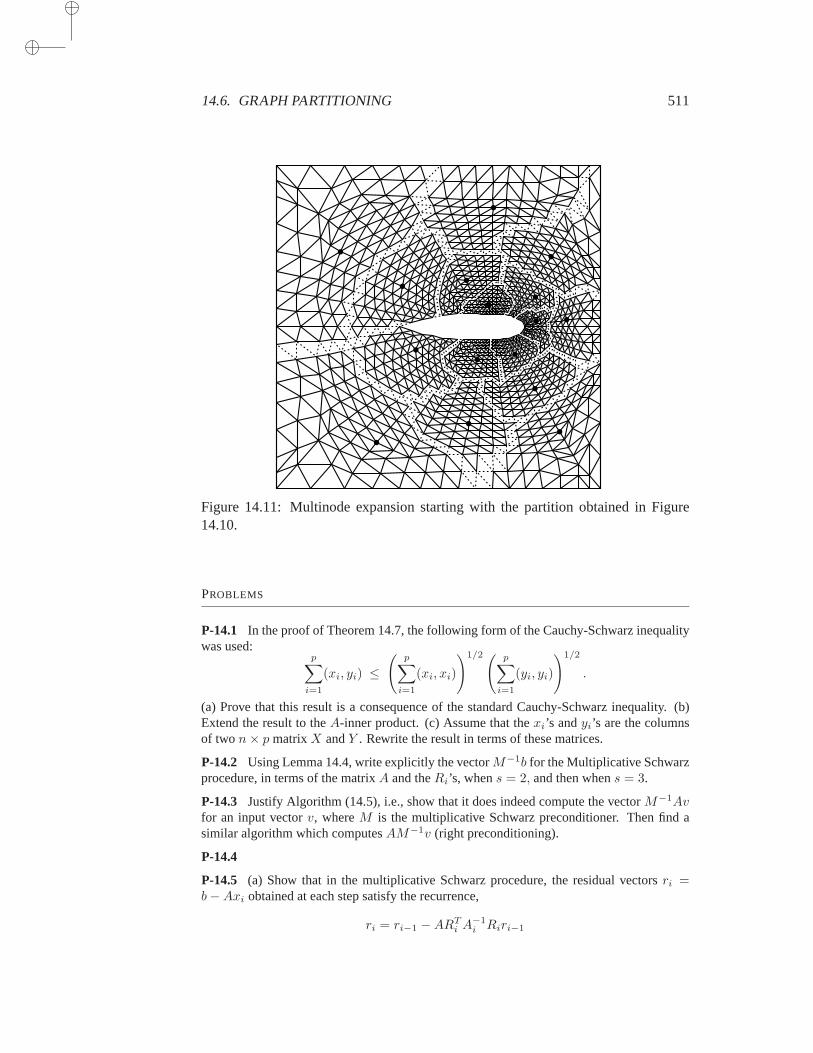
14.6. GRAPH PARTITIONING 511
Figure 14.11: Multinode expansion starting with the partition obtained in Figure14.10.
PROBLEMS
P-14.1 In the proof of Theorem 14.7, the following form of the Cauchy-Schwarz inequalitywas used:
p∑
i=1
(xi, yi) ≤(
p∑
i=1
(xi, xi)
)1/2( p∑
i=1
(yi, yi)
)1/2
.
(a) Prove that this result is a consequence of the standard Cauchy-Schwarz inequality. (b)Extend the result to theA-inner product. (c) Assume that thexi’s andyi’s are the columnsof two n× p matrixX andY . Rewrite the result in terms of these matrices.
P-14.2 Using Lemma 14.4, write explicitly the vectorM−1b for the Multiplicative Schwarzprocedure, in terms of the matrixA and theRi’s, whens = 2, and then whens = 3.
P-14.3 Justify Algorithm (14.5), i.e., show that it does indeed compute the vectorM−1Avfor an input vectorv, whereM is the multiplicative Schwarz preconditioner. Then find asimilar algorithm which computesAM−1v (right preconditioning).
P-14.4
P-14.5 (a) Show that in the multiplicative Schwarz procedure, the residual vectorsri =b−Axi obtained at each step satisfy the recurrence,
ri = ri−1 −ARTi A
−1i Riri−1
512 CHAPTER 14. DOMAIN DECOMPOSITION METHODS
for i = 1, . . . , s. (b) Consider the operatorQi ≡ ARTi A
−1i Ri. Show thatQi is a projector.
(c) IsQi an orthogonal projector with respect to theA-inner product? With respect to whichinner product is it orthogonal?
P-14.6 The analysis of the Additive Schwarz procedure assumes thatA−1i is “exact,” i.e.,
that linear systemsAix = b are solved exactly, each timeA−1i is applied. Assume thatA−1
i
is replaced by some approximationΘ−1i . (a) IsPi still a projector? (b) Show that ifΘi is
Symmetric Positive Definite, then so isPi. (c) Now make the assumption thatλmax(Pi) ≤ω∗. What becomes of the result of Theorem 14.5?
P-14.7 In Element-By-Element (EBE) methods, the extreme cases of the Additive or theMultiplicative Schwarz procedures are considered in whichthe subdomain partition corre-sponds to takingΩi to be an element. The advantage here is that the matrices do not have tobe assembled. Instead, they are kept in unassembled form (see Chapter 2). Assume that Pois-son’s equation is being solved. (a) What are the matricesAi? (b) Are they SPD? (c) Writedown the EBE preconditioning corresponding to the multiplicative Schwarz procedure, itsmulticolor version, and the additive Schwarz procedure.
P-14.8 Theorem 14.2 was stated only for the multiplicative versionof the Schwarz proce-dure. There is a similar result for the additive Schwarz procedure. State this result and proveit.
P-14.9 Show that the matrix defined by (14.38) is indeed a projector.Is it possible to for-mulate Schwarz procedures in terms of projection processesas seen in Chapter 5?
P-14.10 It was stated at the end of the proof of Theorem 14.7 that if
(AJu, u)A ≥1
C(u, u)A
for any nonzerou, thenλmin(AJ ) ≥ 1C . (a) Prove this result without invoking the min-max
theory. (b) Prove a version of the min-max theorem with theA-inner product, i.e., prove thatthe min-max theorem is valid for any inner product for whichA is self-adjoint.
P-14.11 Consider the Laplacean of a graph as defined in Section 14.6. Show that
(Lx, x) =∑
(i,j) ∈ E
(xi − xj)2.
P-14.12 Consider a rectangular finite difference mesh, with mesh size ∆x = h in thex-direction and∆y = h closest to they-direction.
a. To each mesh pointp = (xi, yj), associate the closed diskDij of radiush centered atpi. What is the smallestk such that the familyDij is ak-ply system?
b. Answer the same question for the case where the radius is reduced toh/2. What is theoverlap graph (and associated mesh) for anyα such that
1
2< α <
√2
2?
What about whenα = 2?
P-14.13 Determine the cost of a level set expansion algorithm starting fromp distinct cen-ters.
P-14.14 Write recursive versions of the Recursive Graph Partitioning algorithm and Recur-sive Spectral Bisection algorithm. [Hint: Recall that a recursive program unit is a subpro-gram or function, sayfoo, which calls itself, sofoo is allowed to make a subroutine call to
14.6. GRAPH PARTITIONING 513
foo within its body.] (a) Give a pseudo-code for the RGB algorithm which processes thesubgraphs in any order. (b) Give a pseudo-code for the RGB algorithm case when the largersubgraph is to be processed before the smaller one in any dissection. Is this second versionequivalent to Algorithm 14.9?
P-14.15 Write a FORTRAN-90 subroutine or (C function) which implements the RecursiveGraph Partitioning algorithm.
NOTES AND REFERENCES. To start with, the original paper by Schwarz is the reference [261], but anearlier note appeared in 1870. In recent years, research on DomainDecomposition techniques has beenvery active and productive. This rebirth of an old technique has been inlarge part motivated by parallelprocessing. However, the first practical use of Domain Decompositionideas has been in applicationsto very large structures; see [230, 41], and elasticity problems; see, e.g., [234, 283, 269, 76, 40] forreferences.
The book by Smith, Bjørstad, and Gropp, [268] gives a thorough survey of domain decompositionmethods. Two other monographs, one by P. Le Tallec [198], and the other by C. Farhat and J. X.Roux [123], describe the use of Domain Decomposition approaches specifically for solving problems instructural mechanics. Survey papers include those by Keyes and Gropp [189] and by Chan and Matthew[75]. The volume [190] discusses the various uses of “domain-based” parallelism in computationalsciences and engineering.
The bulk of recent work on Domain Decomposition methods has been geared toward a PartialDifferential Equations viewpoint. Often, there appears to be a dichotomy between this viewpoint andthat of “applied Domain Decomposition,” in that the good methods from a theoretical point of view arehard to implement in practice. The additive Schwarz procedure, with overlapping, represents a com-promise between good intrinsic properties and ease of implementation. Forexample, Venkatakrishnanconcludes in [295] that although the use of global coarse meshes may accelerate convergence of local,domain-based, ILU preconditioners, it does not necessarily reducethe overall time to solve a practicalaerodynamics problem.
Much is known about the convergence of the Schwarz procedure; refer in particular to the work byWidlund and co-authors [42, 102, 103, 104, 70]. The convergenceresults of Section 14.3.4 have beenadapted from Xu [320] as well as Hackbusch [163]. The result on theequivalence between Schwarzand Schur complement iterations stated in Theorem 14.2 seems to have been originally proved by Chanand Goovaerts [73], see also the more recent article by Wilders and Brakkee [315]. The results onthe equivalence between the full matrix techniques and the Schur matrix techniques seen in Section14.5 have been adapted from results by S. E. Eisenstat, reported in [189]. These connections are ratherinteresting and useful in practice since they provide some flexibility on waysto implement a method.A number of preconditioners have also been derived using similar connections in the PDE framework[48, 47, 49, 50, 51].
Research on graph partitioning has slowed in recent years, no doubt due to the appearance ofMetis, a well-designed and efficient graph partitioning code [185]. Variations of the Recursive SpectralBisection algorithm [229] seem to give the best results in terms of overall quality of the subgraphs.However, the algorithm is rather expensive, and the less costly multilevel techniques such as the onesin the codes Metis [185] and Chaco [166], are usually preferred. Thedescription of the geometricpartitioning techniques in Section 14.6.2 is based on the papers [145] and[211]. Earlier approacheshave been developed in [81, 82, 83].

Bibliography
[1] J. ABAFFY AND E. SPEDICATO, ABS Projection Methods, Halstead Press, 1989.
[2] L. M. A DAMS, Iterative algorithms for large sparse linear systems on parallel com-puters, PhD thesis, Applied Mathematics, University of Virginia,Charlottsville, VA,1982. Also NASA Contractor Report 166027.
[3] L. M. A DAMS AND H. JORDAN, Is SOR color-blind?, SIAM Journal on Scientificand Statistical Computing, 6 (1985), pp. 490–506.
[4] L. M. A DAMS AND J. ORTEGA, A multi-color SOR Method for Parallel Computers,in Proceedings of the 1982 International Conference on Pararallel Processing, 1982,pp. 53–56.
[5] J. I. ALIAGA , D. L. BOLEY, R. W. FREUND, AND V. HERNANDEZ, A Lanczos-typealgorithm for multiple starting vectors, Tech. Rep. Numerical Analysis ManuscriptNo 95-11, AT&T Bell Laboratories, Murray Hill, NJ, 1995.
[6] F. L. ALVARADO , Manipulation and visualization of sparse matrices, ORSA Journalon Computing, 2 (1990), pp. 186–206.
[7] E. C. ANDERSON, Parallel implementation of preconditioned conjugate gradientmethods for solving sparse systems of linear equations, Tech. Rep. 805, CSRD, Uni-versity of Illinois, Urbana, IL, 1988. MS Thesis.
[8] E. C. ANDERSON ANDY. SAAD , Solving sparse triangular systems on parallel com-puters., International Journal of High Speed Computing, 1 (1989), pp. 73–96.
[9] W. E. ARNOLDI, The principle of minimized iteration in the solution of the matrixeigenvalue problem, Quart. Appl. Math., 9 (1951), pp. 17–29.
[10] C. C. ASHCRAFT AND R. G. GRIMES, On vectorizing incomplete factorizationand SSOR preconditioners, SIAM Journal on Scientific and Statistical Computing,9 (1988), pp. 122–151.
[11] O. AXELSSON, A generalized SSOR method, BIT, 12 (1972), pp. 443–467.
[12] , Conjugate gradient type-methods for unsymmetric and inconsistent systems oflinear equations, Linear Algebra and its Applications, 29 (1980), pp. 1–16.
[13] , A generalized conjugate gradient, least squares method, Numerische Mathe-matik, 51 (1987), pp. 209–227.
[14] , Iterative Solution Methods, Cambridge University Press, New York, 1994.
[15] O. AXELSSON ANDV. A. BARKER, Finite Element Solution of Boundary Value Prob-lems, Academic Press, Orlando, FL, 1984.
515
516 BIBLIOGRAPHY
[16] O. AXELSSON, S. BRINKKEMPER, AND V. P. ILL’ N, On some versions of incompleteblock-matrix factorization iterative methods, Linear Algebra and its Applications, 58(1984), pp. 3–15.
[17] O. AXELSSON ANDM. NEYTCHEVA, Algebraic multilevel iteration method for stielt-jes matrices, Numer. Linear Algebra Appl., 1 (1994), pp. 213–236.
[18] O. AXELSSON AND B. POLMAN , A robust preconditioner based on algebraic sub-structuring and two-level grids, in Robust multigrid methods. Proc., Kiel, Jan. 1988.,W. Hackbusch, ed., Notes on Numerical Fluid Mechanics, Volume 23, Vieweg, Braun-schweig, 1988, pp. 1–26.
[19] O. AXELSSON AND P. VASSILEVSKI, Algebraic multilevel preconditioning methods.I, Numer. Math., 56 (1989), pp. 157–177.
[20] , A survey of multilevel preconditioned iterative methods, BIT, 29 (1989),pp. 769–793.
[21] , Algebraic multilevel preconditioning methods. II, SIAM J. Numer. Anal., 27(1990), pp. 1569–1590.
[22] O. AXELSSON AND P. S. VASSILEVSKI, A block generalized conjugate gradientsolver with inner iterations and variable step preconditioning, SIAM Journal on Ma-trix Analysis and Applications, 12 (1991).
[23] N. S. BAKHVALOV , On the convergence of a relaxation method with natural con-straints on the elliptic operator, U.S.S.R Computational Math. and Math. Phys., 6(1966), pp. 101–135.
[24] S. BALAY , W. D. GROPP, L. C. MCINNES, AND B. F. SMITH , PETSc 2.0 users man-ual, Tech. Rep. ANL-95/11 - Revision 2.0.24, Argonne National Laboratory, 1999.
[25] R. BANK , T. DUPONT, AND H. YSERENTANT, The hierarchical basis multigridmethod, Numer. Math., 52 (1988), pp. 427–458.
[26] R. BANK AND J. XU, The hierarchical basis multigrid method and incomplete LUdecomposition, tech. rep., U.C. San Diego, Dept. of Math., 1994.
[27] R. E. BANK AND T. F. CHAN, An analysis of the composite step biconjugate gradientmethod, Numerische Mathematik, 66 (1993), pp. 259–319.
[28] R. E. BANK AND C. WAGNER, Multilevel ILU decomposition, Numerische Mathe-matik, 82 (1999), pp. 543–576.
[29] T. BARTH AND T. MANTEUFFEL, Variable metric conjugate gradient methods, inAdvances in Numerical Methods for Large Sparse Sets of Linear Equations, Number10, Matrix Analysis and Parallel Computing, PCG 94, Keio University, Yokohama,Japan, 1994, pp. 165–188.
[30] D. BAXTER, J. SALTZ , M. H. SCHULTZ, S. C. EISENSTAT, AND K. CROWLEY, Anexperimental study of methods for parallel preconditionedKrylov methods, in Pro-ceedings of the 1988 Hypercube Multiprocessors Conference, Pasadena, CA, Jan.1988, pp. 1698–1711.
[31] M. BENANTAR AND J. E. FLAHERTY, A six color procedure for the parallel so-lution of Elliptic systems using the finite quadtree structure, in Proceedings of theFourth SIAM Conference on Parallel Processing for Scientific Computing, J. Don-garra, P. Messina, D. C. Sorenson, and R. G. Voigt, eds., 1990, pp. 230–236.

BIBLIOGRAPHY 517
[32] M. BENZI, J. C. HAWS, AND M. TUMA , Preconditioning highly indefinite and non-symmetric matrices, SIAM Journal on Scientific Computing, 22 (2000), pp. 1333–1353.
[33] M. BENZI, J. MARIN , AND M. TUMA , A two-level parallel preconditioner based onsparse approximate inverses, in Iterative Methods in Scientific Computation, II, D. R.Kincaid and A. C. Elster, eds., IMACS, 1999, pp. xx–xx+10.
[34] M. BENZI, C. D. MEYER, AND M. TUMA , A sparse approximate inverse precondi-tioner for the conjugate gradient method, SIAM Journal on Scientific Computing, 17(1996), pp. 1135–1149.
[35] M. BENZI, D. B. SZYLD , AND A. VAN DUIN, Orderings for incomplete factoriza-tions of nonsymmtric matrices, SIAM Journal on Scientific Computing, 20 (1999),pp. 1652–1670.
[36] M. BENZI AND M. TUMA , A sparse approximate inverse preconditioner for nonsym-metric linear systems, SIAM Journal on Scientific Computing, 19 (1998), pp. 968–994.
[37] H. BERRYMAN, J. SALTZ , W. GROPP, AND R. MIRCHANDANEY, Krylov methodspreconditioned with incompletely factored matrices on theCM-2, Journal of Paralleland Distributed Computing, 8 (1990), pp. 186–190.
[38] G. BIRKHOFF, R. S. VARGA, AND D. M. YOUNG, Alternating direction implicitmethods, in Advances in Computers, F. Alt and M. Rubinov, eds., New York, 1962,Academic Press, pp. 189–273.
[39] A. BJORCK AND T. ELFVING, Accelerated projection methods for computing pseudo-inverse solutions of systems of linear equations, BIT, 19 (1979), pp. 145–163.
[40] P. E. BJØRSTAD AND A. HVIDSTEN, Iterative methods for substructured elasticityproblems in structural analysis, in Domain Decomposition Methods for Partial Dif-ferential Equations, R. Glowinski, G. H. Golub, G. A. Meurant, and J. Periaux, eds.,Philadelphia, PA, 1988, SIAM.
[41] P. E. BJØRSTAD AND O. B. WIDLUND , Solving elliptic problems on regions parti-tioned into substructures, in Elliptic Problem Solvers II, G. Birkhoff and A. Schoen-stadt, eds., New York, NY, 1984, Academic Press, pp. 245–256.
[42] , Iterative methods for the solution of elliptic problems on regions partitionedinto substructures, SIAM Journal on Numerical Analysis, 23 (1986), pp. 1093–1120.
[43] E. BODEWIG, Matrix Calculus, North-Holland, Amsterdam, 1956.
[44] M. BOLLHOFER, A robust ILU with pivoting based on monitoring the growth of theinverse factors, Linear Algebra and its Applications, 338 (2001), pp. 201–213.
[45] E. BOTTA, A. PLOEG, AND F. WUBS, Nested grids ILU-decomposition (NGILU), J.Comp. Appl. Math., 66 (1996), pp. 515–526.
[46] H. BRAKHAGE, Uber die numerische Behandlung von integralgleichungen nach derQuadratureformelmethode, Numerische Mathematik, 2 (1960), pp. 183–196.
[47] J. H. BRAMBLE , J. E. PASCIAK , AND A. H. SCHATZ, The construction of precon-ditioners for elliptic problems by substructuring, I, Mathematics of Computation, 47(1986), pp. 103–134.
518 BIBLIOGRAPHY
[48] , An iterative method for elliptic problems on regions partitioned into substruc-tures, Mathematics of Computation, 46 (1986), pp. 361–369.
[49] , The construction of preconditioners for elliptic problemsby substructuring, II,Mathematics of Computation, 49 (1987), pp. 1–16.
[50] , The construction of preconditioners for elliptic problemsby substructuring, III,Mathematics of Computation, 51 (1988), pp. 415–430.
[51] , The construction of preconditioners for elliptic problemsby substructuring, IV,Mathematics of Computation, 53 (1989), pp. 1–24.
[52] R. BRAMLEY AND A. SAMEH, Row projection methods for large nonsymmetriclinear systems, SIAM Journal on Scientific and Statistical Computing, 13 (1992),pp. 168–193.
[53] , A robust parallel solver for block tridiagonal systems, in Proceedings of theInternational Conference on Supercomputing, ACM, July 1988, pp. 39–54.
[54] A. BRANDT, Multi-level adaptive technique (MLAT) for fast numerical solutions toboundary problems., in Proc. 3rd Int. Conf. Numer. Methods in Fluid Mechanics,Paris, 1972, H. Cabannes and R. Temam, eds., Berlin, 1973, Springer Verlag, pp. 82–89.
[55] , Multi-level adaptive solutions to boundary value problems, Mathematics ofComputation, 31 (1977), pp. 333–390.
[56] , A guide to multigrid development, in Multigrid methods, W. Hackbusch andU. Trottenberg, eds., Berlin, 1982, Springer Verlag, pp. 220–312.
[57] , Algebraic multigrid theory: The symmetric case, Appl. Math. Comp., 19(1985).
[58] A. BRANDT, S. F. MC CORMICK, AND J. RUGE, Algebraic multigrid (amg) forsparse matrix equations, in Sparsity and its applications, D. J. Evans, ed., Cambridge,1984, Cambridge Univ. Press.
[59] C. BREZINSKI, Pade Type Approximation and General Orthogonal Polynomials,Birkhauser-Verlag, Basel-Boston-Stuttgart, 1980.
[60] C. BREZINSKI AND M. REDIVO ZAGLIA , Extrapolation Methods: Theory and Prac-tice, North-Holland, Amsterdam, 1991.
[61] C. BREZINSKI AND M. REDIVO-ZAGLIA , Hybrid procedures for solving systems oflinear equations, Numerische Mathematik, 67 (1994), pp. 1–19.
[62] C. BREZINSKI, M. REDIVO-ZAGLIA , AND H. SADOK, Avoiding breakdownand near-breakdown in Lanczos-type algorithms, Numerical Algorithms, 1 (1991),pp. 261–284.
[63] , A breakdown-free Lanczos-type algorithm for solving linear systems, Nu-merische Mathematik, 63 (1992), pp. 29–38.
[64] R. BRIDSON AND W. P. TANG, Ordering, anisotropy, and factored sparse approxi-mate inverses, SIAM Journal on Scientific Computing, 21 (1999).
[65] W. L. BRIGGS, V. E. HENSON, AND S. F. MC CORMICK, A multigrid tutorial,SIAM, Philadelphia, PA, 2000. Second edition.
BIBLIOGRAPHY 519
[66] P. N. BROWN, A theoretical comparison of the Arnoldi and GMRES algorithms,SIAM Journal on Scientific and Statistical Computing, 12 (1991), pp. 58–78.
[67] P. N. BROWN AND A. C. HINDMARSH, Matrix-free methods for stiff systems ofODEs, SIAM Journal on Numerical Analysis, 23 (1986), pp. 610–638.
[68] N. I. BULEEV, A numerical method for the solution of two-dimensional and three-dimensional equations of diffusion, Math. Sb, 51 (1960), pp. 227–238. (in Russian).
[69] O. BUNEMAN, A compact non-iterative Poisson solver, Tech. Rep. 294, Stanford Uni-versity, Stanford, CA, 1969.
[70] X. C. CAI AND O. WIDLUND , Multiplicative Schwarz algorithms for some nonsym-metric and indefinite problems, SIAM Journal on Numerical Analysis, 30 (1993).
[71] L. CESARI, Sulla risoluzione dei sistemi di equazioni lineari per approssimazionisuccessive, Atti Accad. Naz. Lincei Rend. Cl. Sci. Fis. Mat. Nat., Ser. 6a, 25 (1937),pp. 422–428.
[72] T. F. CHAN , E. GALLOPOULOS, V. SIMONCINI , T. SZETO, AND C. TONG, A quasi-minimal residual variant of the Bi-CGSTAB algorithm for nonsymmetric systems,SIAM Journal on Scientific Computing, 15 (1994), pp. 338–347.
[73] T. F. CHAN AND D. GOOVAERTS, On the relationship between overlapping andnonoverlapping domain decomposition methods, SIAM Journal on Matrix Analysisand Applications, 13 (1992), pp. 663–670.
[74] T. F. CHAN AND T. P. MATHEW, The interface probing technique in domain decom-position, SIAM Journal on Matrix Analysis and Applications, 13 (1992), pp. 212–238.
[75] , Domain decomposition algorithms, Acta Numerica, (1994), pp. 61–143.
[76] H. C. CHEN AND A. SAMEH, A matrix decomposition method for orthotropic elastic-ity problems, SIAM Journal on Matrix Analysis and Applications, 10 (1989), pp. 39–64.
[77] C. C. CHENEY, Introduction to Approximation Theory, McGraw Hill, NY, 1966.
[78] E. CHOW AND Y. SAAD , Approximate inverse techniques for block-partitioned ma-trices, SIAM Journal on Scientific Computing, 18 (1997), pp. 1657–1675.
[79] , ILUS: an incomplete LU factorization for matrices in sparseskyline format,International Journal for Numerical Methods in Fluids, 25 (1997), pp. 739–748.
[80] , Approximate inverse preconditioners via sparse-sparse iterations, SIAM Jour-nal on Scientific Computing, 19 (1998), pp. 995–1023.
[81] N. CHRISOCHOIDES, G. FOX, AND J. THOMPSON, MENUS-PGG mapping environ-ment for numerical unstructured and structured parallel grid generation, in Proceed-ings of the Seventh International Conference on Domain Decomposition Methods inScientific and Engineering Computing, 1993.
[82] N. CHRISOCHOIDES, C. E. HOUSTIS, E. N. HOUSTIS, P. N. PAPACHIOU, S. K.KORTESIS, AND J. RICE, DOMAIN DECOMPOSER: a software tool for mappingPDE computations to parallel architectures, in Domain Decomposition Methods forPartial Differential Equations, R. G. et. al., ed., SIAM publications, 1991, pp. 341–357.
520 BIBLIOGRAPHY
[83] N. CHRISOCHOIDES, E. HOUSTIS, AND J. RICE, Mapping algorithms and soft-ware environment for data parallel PDE iterative solvers, Journal of Parallel and Dis-tributed Computing, 21 (1994), pp. 75–95.
[84] P. G. CIARLET, The finite element method for elliptic problems, North-Holland, Am-sterdam, 1978.
[85] G. CIMMINO , Calcolo approssimato per le soluzioni dei sistemi di equazioni lineari,Ricerca Scientifica, II, 9 (1938), pp. 326–333.
[86] A. CLAYTON , Further results on polynomials having least maximum modulus over anellipse in the complex plane, Tech. Rep. AEEW-7348, UKAEA, Harewell-UK, 1963.
[87] S. CLIFT AND W. TANG, Weighted graph based ordering techniques for precondi-tioned conjugate gradient methods, BIT, 35 (1995), pp. 30–47.
[88] P. CONCUS AND G. H. GOLUB, A generalized conjugate gradient method for non-symmetric systems of linear equations, in Computing Methods in Applied Sciencesand Engineering, R. Glowinski and J. L. Lions, eds., New York, 1976, Springer Ver-lag, pp. 56–65.
[89] P. CONCUS, G. H. GOLUB, AND G. MEURANT, Block preconditioning for the con-jugate gradient method, SIAM Journal on Scientific and Statistical Computing, 6(1985), pp. 220–252.
[90] T. H. CORMEN, C. E. LEISERSON, AND R. L. RIVEST, Introduction to Algorithms,Mc Graw Hill, New York, 1990.
[91] J. D. F. COSGROVE, J. C. DIAZ , AND A. GRIEWANK, Approximate inverse precon-ditioning for sparse linear systems, Interernaitonal Journal of Computational Mathe-matics, 44 (1992), pp. 91–110.
[92] J. CULLUM AND A. GREENBAUM, Relations between Galerkin and norm-minimizingiterative methods for solving linear systems, SIAM Journal on Matrix Analysis andApplications, 17 (1996), pp. 223–247.
[93] B. N. DATTA , Numerical Linear Algebra and Applications, second edition, SIAM,Philadelphia, PA, 2010.
[94] P. J. DAVIS, Interpolation and Approximation, Blaisdell, Waltham, MA, 1963.
[95] T. A. DAVIS, A parallel algorithm for sparse unsymmetric LU factorizations, PhDthesis, University of Illinois at Urbana Champaign, Urbana, IL., 1989.
[96] E. F. D’AZEVEDO, F. A. FORSYTH, AND W. P. TANG, Ordering methods for pre-conditioned conjugate gradient methods applied to unstructured grid problems, SIAMJournal on Matrix Analysis and Applications, 13 (1992), pp.944–961.
[97] , Towards a cost effective ILU preconditioner with high levelfill , BIT, 31 (1992),pp. 442–463.
[98] M. A. DELONG AND J. M. ORTEGA, SOR as a preconditioner, Applied NumericalMathematics, 18 (1995), pp. 431–440.
[99] J. W. DEMMEL, Applied Numerical Linear Algebra, SIAM, Philadelphia, PA, 1997.
[100] P. DEUFLHARD, R. W. FREUND, AND A. WALTER, Fast secant methods for theiterative solution of large nonsymmetric linear systems, IMPACT of Computing inScience and Engineering, 2 (1990), pp. 244–276.
BIBLIOGRAPHY 521
[101] J. J. DONGARRA, I. S. DUFF, D. SORENSEN, AND H. A. VAN DER VORST, SolvingLinear Systems on Vector and Shared Memory Computers, SIAM, Philadelphia, PA,1991.
[102] M. DRYJA AND O. B. WIDLUND , Some domain decomposition algorithms for ellipticproblems, in Iterative Methods for Large Linear Systems, L. Hayes andD. Kincaid,eds., New York, NY, 1989, Academic Press, pp. 273–291.
[103] , Towards a unified theory of domain decomposition algorithmsfor ellipticproblems, in Third International Symposium on Domain DecompositionMethods forPartial Differential Equations, held in Houston, TX, March20-22, 1989, T. Chan,R. Glowinski, J. Periaux, and O. Widlund, eds., Philadelphia, PA, 1990, SIAM.
[104] , Additive Schwarz methods for elliptic finite element problems in three dimen-sions, in Fifth International Symposium on Domain DecompositionMethods for Par-tial Differential Equations, T. F. Chan, D. E. Keyes, G. A. Meurant, J. S. Scroggs, andR. G. Voigt, eds., Philadelphia, PA, 1992, SIAM.
[105] P. F. DUBOIS, A. GREENBAUM, AND G. H. RODRIGUE, Approximating the inverseof a matrix for use on iterative algorithms on vectors processors, Computing, 22(1979), pp. 257–268.
[106] I. S. DUFF, A survey of sparse matrix research, in Proceedings of the IEEE, 65, NewYork, 1977, Prentice Hall, pp. 500–535.
[107] I. S. DUFF, A. M. ERISMAN, AND J. K. REID, Direct Methods for Sparse Matrices,Clarendon Press, Oxford, 1986.
[108] I. S. DUFF, R. G. GRIMES, AND J. G. LEWIS, Sparse matrix test problems, ACMTransactions on Mathematical Software, 15 (1989), pp. 1–14.
[109] I. S. DUFF AND J. KOSTER, The design and use of algorithms for permuting largeentries to the diagonal of sparse matrices, SIAM Journal on Matrix Analysis andApplications, 20 (1999), pp. 889–901.
[110] , On algorithms for permuting large entries to the diagonal ofa sparse matrix,SIAM Journal on Matrix Analysis and Applications, 22 (2001), pp. 973–996.
[111] I. S. DUFF AND G. A. MEURANT, The effect of ordering on preconditioned conjugategradients, BIT, 29 (1989), pp. 635–657.
[112] L. C. DUTTO, The effect of reordering on the preconditioned GMRES algorithm forsolving the compressible Navier-Stokes equations, International Journal for NumericalMethods in Engineering, 36 (1993), pp. 457–497.
[113] T. EIROLA AND O. NEVANLINNA , Accelerating with rank-one updates, Linear Alge-bra and its Applications, 121 (1989), pp. 511–520.
[114] S. EISENSTAT, Efficient implementation of a class of conjugate gradient methods,SIAM Journal on Scientific and Statistical Computing, 2 (1988), pp. 1–4.
[115] S. C. EISENSTAT, M. H. SCHULTZ, AND A. H. SHERMAN, Algorithms and datastructures for sparse symmetric Gaussian elimination, SIAM Journal on ScientificComputing, 2 (1981), pp. 225–237.
[116] H. C. ELMAN , A stability analysis of incomplete LU factorizations, Mathematics ofComputation, 47 (1986), pp. 191–217.
522 BIBLIOGRAPHY
[117] H. C. ELMAN AND E. AGRON, Ordering techniques for the preconditioned conju-gate gradient method on parallel computers, Computer Physics Communications, 53(1989), pp. 253–269.
[118] H. C. ELMAN AND G. H. GOLUB, Inexact and preconditioned Uzawa algorithms forsaddle point problems, SIAM Journal on Numerical Analysis, 31 (1994), pp. 1645–1661.
[119] H. C. ELMAN AND D. J. SILVESTER, Fast nonsymmetric iteration and precondition-ing for Navier-Stokes equations, SIAM Journal on Scientific Computing, 17 (1996),pp. 33–46.
[120] M. ENGLEMAN, FIDAP manuals, Tech. Rep. Vol. 1, 2, and 3, Fluid Dynamics Inter-national, Evanston, IL, 1986.
[121] V. FABER AND T. MANTEUFFEL, Necessary and sufficient conditions for the ex-istence of a conjugate gradient method, SIAM Journal on Numerical Analysis, 21(1984), pp. 352–361.
[122] K. FAN, Note onM -matrices, Quarterly Journal of Mathematics, Oxford series (2),11 (1960), pp. 43–49.
[123] C. FARHAT AND F. X. ROUX, Implicit parallel processing in structural mechanics,Computational Mechanics Advances, 2 (1994), pp. 1–124.
[124] R. P. FEDORENKO, A relaxation method for solving elliptic difference equations,U.S.S.R Computational Math. and Math. Phys., 1 (1962), pp. 1092–1096.
[125] , The speed of convergence of one iterative process, U.S.S.R ComputationalMath. and Math. Phys., 4 (1964), pp. 227–235.
[126] R. M. FERENCZ, Element-by-element preconditioning techniques for largescale vec-torized finite element analysis in nonlinear solid and structural mechanics, PhD thesis,Department of Applied Mathematics, Stanford, CA, 1989.
[127] B. FISCHER AND R. W. FREUND, On the constrained Chebyshev approximationproblem on ellipses, Journal of Approximation Theory, 62 (1990), pp. 297–315.
[128] , Chebyshev polynomials are not always optimal, Journal of Approximation The-ory, 65 (1991), pp. 261–272.
[129] B. FISCHER AND L. REICHEL, A stable Richardson iteration method for complexlinear systems, Numerische Mathematik, 54 (1988), pp. 225–241.
[130] R. FLETCHER, Conjugate gradient methods for indefinite systems, in Proceedings ofthe Dundee Biennal Conference on Numerical Analysis 1974, G. A. Watson, ed., NewYork, 1975, Springer Verlag, pp. 73–89.
[131] I. T. FOSTER, Designing and Building Parallel Programs: Concepts and Tools forParallel Software Engineering, Addison-Wesley, 1995.
[132] R. W. FREUND, Conjugate gradient-type methods for linear systems with complexsymmetric coefficient matrices, SIAM Journal on Scientific and Statistical Computing,13 (1992), pp. 425–448.
[133] , Quasi-kernel polynomials and convergence results for quasi-minimal residualiterations, in Numerical Methods of Approximation Theory, Vol 9, D. Braess andL. L. Schumaker, eds., International series of numerical mathematics, Basel, 1992,Birkhauser Verlag, pp. 1–19.
BIBLIOGRAPHY 523
[134] , A Transpose-Free Quasi-Minimal Residual algorithm for non-Hermitian linearsystems, SIAM Journal on Scientific Computing, 14 (1993), pp. 470–482.
[135] R. W. FREUND, M. H. GUTKNECHT, AND N. M. NACHTIGAL , An implementationof of the Look-Ahead Lanczos algorithm, SIAM Journal on Scientific and StatisticalComputing, 14 (1993), pp. 470–482.
[136] R. W. FREUND AND N. M. NACHTIGAL , QMR: a quasi-minimal residual methodfor non-Hermitian linear systems, Numerische Mathematik, 60 (1991), pp. 315–339.
[137] K. GALLIVAN , A. SAMEH , AND Z. ZLATEV , A parallel hybrid sparse linear systemsolver, Computing Systems in Engineering, 1 (June 1990), pp. 183–195.
[138] E. GALLOPOULOS AND Y. SAAD , Parallel block cyclic reduction algorithm for thefast solution of elliptic equations, Parallel Comput., 10 (1989), pp. 143–160.
[139] F. R. GANTMACHER, The Theory of Matrices, Chelsea, New York, 1959.
[140] N. GASTINEL, Analyse Numerique Lineaire, Hermann, Paris, 1966.
[141] W. GAUTSCHI, On generating orthogonal polynomials, SIAM Journal on Scientificand Statistical Computing, 3 (1982), pp. 289–317.
[142] A. GEORGE, Computer implementation of the finite element method, Tech. Rep.STAN-CS-208, Stanford University, Department of ComputerScience, 1971.
[143] A. GEORGE ANDJ. W.-H. LIU, The evolution of the minimum degree ordering algo-rithm, SIAM Review, 31 (March 1989), pp. 1–19.
[144] J. A. GEORGE AND J. W. LIU, Computer Solution of Large Sparse Positive DefiniteSystems, Prentice-Hall, Englewood Cliffs, NJ, 1981.
[145] J. R. GILBERT, G. L. MILLER , AND S.-H. TENG, Geometric mesh partitioning:Implementation and experiments, in IPPS 94, Submitted to SIAM SISC, 1995.
[146] J. R. GILBERT AND T. PEIERLS, Sparse partial pivoting in time proportional to ar-tithmetic operations, SIAM Journal on Scientific Computing, 9 (1988), pp. 862–874.
[147] S. K. GODUNOV AND G. P. PROPKOPOV, A method of minimal iteration for eval-uating the eigenvalues of an elliptic operator, Zh. Vichsl. Mat. Mat. Fiz., 10 (1970),pp. 1180–1190.
[148] T. GOEHRING AND Y. SAAD , Heuristic algorithms for automatic graph partitioning,Tech. Rep. umsi-94-29, University of Minnesota Supercomputer Institute, Minneapo-lis, MN, February 1994.
[149] G. H. GOLUB AND C. F. V. LOAN, Matrix Computations, Johns Hopkins UniversityPress, Baltimore, MD, 3rd ed., 1996.
[150] G. H. GOLUB AND M. L. OVERTON, The convergence of inexact Chebyshev andRichardson iterative methods for solving linear systems, Numerische Mathematik, 53(1988), pp. 571–593.
[151] G. H. GOLUB AND R. S. VARGA, Chebyshev semi iterative methods successiveoverrelaxation iterative methods and second order Richardson iterative methods, Nu-merische Mathematik, 3 (1961), pp. 147–168.
[152] G. H. GOLUB AND A. J. WATHENS, An iteration for indefinite systems and its ap-plication to the Navier-Stokes equations, SIAM Journal on Scientific Computing, 19(1998), pp. 530–539.
524 BIBLIOGRAPHY
[153] G. H. GOLUB AND Q. YE, Inexact preconditioned conjugate gradient method withinner-outer iterations, SIAM Journal on Scientific Computing, 21 (1999).
[154] A. GREENBAUM, Iterative Methods for Solving Linear Systems, SIAM, Philadelpha,PA, 1997.
[155] A. GREENBAUM, C. LI , AND H. Z. CHAO, Parallelizing preconditioned conjugategradient algorithms, Computer Physics Communications, 53 (1989), pp. 295–309.
[156] W. GROPP, E. LUSK, AND A. SKJELLUM, Using MPI: Portable Parallel Program-ming with the Message Passing Interface, MIT press, 1994.
[157] M. GROTE AND T. HUCKLE, Effective parallel preconditioning with sparse approxi-mate inverses, in Proceedings of the Seventh SIAM Conference on Parallel Processingfor Scientific Computing, D. H. Bailey, ed., Philadelphia, 1995, SIAM, pp. 466–471.
[158] M. GROTE AND H. D. SIMON, Parallel preconditioning and approximate inverses onthe connection machine, in Parallel Processing for Scientific Computing – vol. 2, R.F.Sincovec, D. E. Keyes, L. R. Petzold, and D. A. Reed, eds., SIAM, 1992, pp. 519–523.
[159] M. J. GROTE AND T. HUCKLE, Parallel preconditionings with sparse approximateinverses, SIAM Journal on Scientific Computing, 18 (1997), pp. 838–853.
[160] M. H. GUTKNECHT, A completed theory of the unsymmetric Lanczos process andrelated algorithms. Part I., SIAM Journal on Matrix Analysis and Applications, 13(1992), pp. 594–639.
[161] , A completed theory of the unsymmetric Lanczos process and related algo-rithms. Part II., SIAM Journal on Matrix Analysis and Applications, 15 (1994),pp. 15–58.
[162] W. HACKBUSCH, Multi-Grid Methods and Applications, vol. 4 of Springer Series inComputational Mathematics, Springer-Verlag, Berlin, 1985.
[163] W. HACKBUSCH, Iterative Solution of Large Linear Systems of Equations, SpringerVerlag, New York, 1994.
[164] P. R. HALMOS, Finite-Dimensional Vector Spaces, Springer Verlag, New York, 1958.
[165] S. HAMMOND AND R. SCHREIBER, Efficient iccg on a shared memory multipro-cessor, Tech. Rep. 89. 24, RIACS, NASA Ames research center, Moffett Field CA.,1989.
[166] B. HENDRICKSON AND R. LELAND, The Chaco User’s Guide Version 2, SandiaNational Laboratories, Albuquerque NM, 1994.
[167] M. R. HESTENES ANDE. L. STIEFEL, Methods of conjugate gradients for solvinglinear systems, Journal of Research of the National Bureau of Standards, Section B,49 (1952), pp. 409–436.
[168] C. HIRSCH, Numerical Computation of Internal and External Flows, John Wiley andSons, New York, 1988.
[169] R. W. HOCKNEY, A fast direct solution of Poisson’s equation using Fourier analysis,J. Assoc. Comput. Mach., 12 (1965), pp. 95–113.
[170] , The potential calculation and some applications, Meth. Comput. Phy., 9(1970), pp. 135–211.
BIBLIOGRAPHY 525
[171] , The potential calculation and some applications, Methods Comput. Phys., 9(1970), pp. 135–211.
[172] R. A. HORN AND C. R. JOHNSON, Matrix Analysis, Cambridge University Press,Cambridge, 1985.
[173] A. S. HOUSEHOLDER, Theory of Matrices in Numerical Analysis, Blaisdell Pub. Co.,Johnson, CO, 1964.
[174] T. J. R. HUGHES, R. M. FERENCZ, AND J. O. HALLQUIST, Large-scale vectorizedimplicit calculations in solid mechanics on a Cray X-MP/48 utilizing EBE precondi-tioned conjugate gradients, Computer Methods in Applied Mechanics and Engineer-ing, 61 (1987), pp. 215–248.
[175] K. JBILOU, Projection minimization methods for nonsymmetric linear systems. Toappear, Linear Algebra and its Applications.
[176] K. JBILOU , A. MESSAOUDI, AND H. SADOK, Global FOM and GMRES algorithmsfor matrix equations, Applied Numerical Mathematics, 31 (1999), pp. 49–63.
[177] K. JBILOU AND H. SADOK, Analysis of some vector extrapolation methods for solv-ing systems of linear equations, Numerische Mathematik, (1995), pp. 73–89.
[178] K. C. JEA AND D. M. YOUNG, Generalized conjugate gradient acceleration ofnonsymmetrizable iterative methods, Linear Algebra and its Applications, 34 (1980),pp. 159–194.
[179] C. JOHNSON, Numerical Solutions of Partial Differential Equations by the Finite El-ement Method, Cambridge University Press, Cambridge, UK, 1987.
[180] O. G. JOHNSON, C. A. MICCHELLI , AND G. PAUL , Polynomial preconditioningsfor conjugate gradient calculations, SIAM Journal on Numerical Analysis, 20 (1983),pp. 362–376.
[181] S. KACZMARZ, Angenaherte auflosung von systemen linearer gleichungen, Bulletininternational de l’Academie polonaise des Sciences et Lettres, III, class A (1937),pp. 355–357.
[182] C. KAMATH AND A. SAMEH, A projection method for solving nonsymmetric linearsystems on multiprocessors, Parallel Computing, 9 (1988), pp. 291–312.
[183] R. M. KARP, Reducibility among combinatorial problems, in Complexity of Com-puter Computations, New York, 1972, Plenum Press, pp. 85–104.
[184] T. I. KARUSH, N. K. MADSEN, AND G. H. RODRIGUE, Matrix multiplication bydiagonals on vector/parallel processors, Tech. Rep. UCUD, Lawrence Livermore Na-tional Lab., Livermore, CA, 1975.
[185] G. KARYPIS AND V. K UMAR, A fast and high quality multilevel scheme for partition-ing irregular graphs, SIAM Journal on Scientific Computing, 20 (1999), pp. 359–392.
[186] C. T. KELLY , Iterative methods for linear and nonlinear equations, SIAM, Philadel-phia, 1995.
[187] D. S. KERSHAW, The incomplete Choleski conjugate gradient method for the iterativesolution of systems of linear equations, Journal of Computational Physics, 26 (1978),pp. 43–65.
526 BIBLIOGRAPHY
[188] R. KETTLER, Analysis and comparison of relaxation schemes in robust multigrid andpreconditioned conjugate gradient methods, in Multigrid methods: Proc., Koln-Porz,Nov. 1981, W. Hackbusch and U. Trottenberg, eds., Lecture notes in Math. 1228,Springer Verlag, Berlin, 1982, pp. 502–534.
[189] D. E. KEYES AND W. D. GROPP, A comparison of domain decomposition techniquesfor elliptic partial differential equations and their parallel implementation, SIAMJournal on Scientific and Statistical Computing, 8 (1987), pp. s166–s202.
[190] D. E. KEYES, Y. SAAD , AND D. G. TRUHLAR, Domain-Based Parallelism andProblem Decomposition Methods in Computational Science and Engineering, SIAM,Philadelphia, PA, 1995. (Conference proceedings).
[191] L. Y. KOLOTILINA AND A. Y. Y EREMIN, On a family of two-level preconditioningsof the incomplete block factorization type, Soviet Journal of Numerical Analysis andMathematical Modeling, 1 (1986), pp. 293–320.
[192] M. A. KRASNOSELSKII ET AL., Approximate Solutions of Operator Equations,Wolters-Nordhoff, Groningen, 1972.
[193] L. KRONSJO AND G. DAHLQUIST, On the design of nested iterations for ellipticdifference equations, BIT, 11 (1971), pp. 63–71.
[194] V. KUMAR , A. GRAMA , A. GUPTA, AND G. KAPYRIS, Parallel Computing, 2ndedition, Benjamin Cummings, Redwood City, CA, 2003.
[195] C. LANCZOS, An iteration method for the solution of the eigenvalue problem of lineardifferential and integral operators, Journal of Research of the National Bureau ofStandards, 45 (1950), pp. 255–282.
[196] , Chebyshev polynomials in the solution of large-scale linear systems, in Pro-ceedings of the ACM, 1952, pp. 124–133.
[197] , Solution of systems of linear equations by minimized iterations, Journal ofResearch of the National Bureau of Standards, 49 (1952), pp.33–53.
[198] P. LETALLEC, Domain decomposition methods in computational mechanics, Compu-tational Mechanics Advances, 1 (1994), pp. 121–220.
[199] R. LEUZE, Independent set orderings for parallel matrix factorizations by Gaussianelimination, Parallel Computing, 10 (1989), pp. 177–191.
[200] J. G. LEWIS, B. W. PEYTON, AND A. POTHEN, A fast algorithm for reorderingsparse matrices for parallel factorizations, SIAM Journal on Scientific and StatisticalComputing, 6 (1989), pp. 1146–1173.
[201] J. G. LEWIS AND H. D. SIMON, The impact of hardware scatter-gather on sparseGaussian elimination, SIAM Journal on Scientific and Statistical Computing, 9(1988), pp. 304–311.
[202] N. LI , Y. SAAD , AND E. CHOW, Crout versions of ILU for general sparse matrices,SIAM Journal on Scientific Computing, 25 (2003), pp. 716–728.
[203] Z. LI , Y. SAAD , AND M. SOSONKINA, pARMS: a parallel version of the algebraic re-cursive multilevel solver, Tech. Rep. umsi-2001-100, Minnesota Supercomputer Insti-tute, University of Minnesota, Minneapolis, MN, 2001. Appeared in NLAA, 10:485-509 (2003).
BIBLIOGRAPHY 527
[204] J. W.-H. LIU, Modification of the minimum degree algorithm by multiple elimination,ACM Transactions on Mathematical Software, 11 (1985), pp. 141–153.
[205] S. MA, Parallel block preconditioned Krylov subspace methods forPartial Differ-ential Equations, PhD thesis, Department of Computer Science, Minneapolis,MN,1993.
[206] T. A. MANTEUFFEL, An incomplete factorization technique for positive definite linearsystems, Mathematics of Computation, 34 (1980), pp. 473–497.
[207] S. F. MC CORMICK, ed.,Multigrid Methods, Philadelphia, PA, 1987, SIAM.
[208] J. A. MEIJERINK AND H. A. VAN DER VORST, An iterative solution method forlinear systems of which the coefficient matrix is a symmetricM-matrix, Mathematicsof Computation, 31 (1977), pp. 148–162.
[209] G. MEURANT, Computer solution of large linear systems, North-Holland, Amster-dam, 1999. Vol 28, Studies in Mathematics and its Applications.
[210] C. D. MEYER, Matrix Analysis and Applied Linear Algebra, SIAM, Philadelphia, PA,2000.
[211] G. L. MILLER , S. H. TENG, W. THURSTON, AND S. A. VAVASIS, Automatic meshpartitioning, in Sparse Matrix Computations: Graph Theory Issues and Algorithms,A. George, J. Gilbert, and J. Liu, eds., 1993. IMA Volumes in Mathematics and ItsApplications.
[212] N. MUNKSGAARD, Solving sparse symmetric sets of linear equations by precondi-tioned conjugate gradient method, ACM Transactions on Mathematical Software, 6(1980), pp. 206–219.
[213] N. M. NACHTIGAL , A look-ahead variant of the Lanczos Algorithm and its applica-tion to the Quasi-Minimal Residual method for non-Hermitian linear systems, PhDthesis, Applied Mathematics, Cambridge, 1991.
[214] Y. NOTAY, Flexible conjugate gradient, SIAM Journal on Scientific Computing, 22(2000), p. 1444=1460.
[215] D. O’LEARY, The block conjugate gradient algorithm and related methods, LinearAlgebra and its Applications, 29 (1980), pp. 243–322.
[216] C. W. OOSTERLEE ANDT. WASHIO, An evaluation of parallel multigrid as a solverand a preconditioner for singularly perturbed problems, SIAM Journal on Scientificand Statistical Computing, 19 (1991), pp. 87–110.
[217] J. ORTEGA, Efficient implementation of certain iterative methods, SIAM Journal onScientific and Statistical Computing, 9 (1988), pp. 882–891.
[218] , Orderings for conjugate gradient preconditionings, SIAM Journal on Scientificand Statistical Computing, 12 (1991), pp. 565–582.
[219] J. M. ORTEGA, Introduction to Parallel and Vector Solution of Linear Systems,Plenum Press, New York, 1988.
[220] J. M. ORTEGA AND R. G. VOIGT, Solution of partial differential equations on vectorand parallel computers, SIAM Review, 27 (1985), pp. 149–240.
[221] O. OSTERBY AND Z. ZLATEV , Direct Methods for Sparse Matrices, Springer Verlag,New York, 1983.
528 BIBLIOGRAPHY
[222] C. C. PAIGE, Computational variants of the Lanczos method for the eigenproblem,Journal of the Institute of Mathematics and its Applications, 10 (1972), pp. 373–381.
[223] C. C. PAIGE AND M. A. SAUNDERS, Solution of sparse indefinite systems of linearequations, SIAM Journal on Numerical Analysis, 12 (1975), pp. 617–624.
[224] B. N. PARLETT, The Symmetric Eigenvalue Problem, no. 20 in Classics in AppliedMathematics, SIAM, Philadelphia, 1998.
[225] B. N. PARLETT, D. R. TAYLOR , AND Z. S. LIU, A look-ahead Lanczos algorithmfor nonsymmetric matrices, Mathematics of Computation, 44 (1985), pp. 105–124.
[226] D. PEACEMAN AND H. RACHFORD, The numerical solution of elliptic and parabolicdifferential equations, Journal of SIAM, 3 (1955), pp. 28–41.
[227] S. PISSANETZKY, Sparse Matrix Technology, Academic Press, New York, 1984.
[228] E. L. POOLE AND J. M. ORTEGA, Multicolor ICCG methods for vector computers,SIAM Journal on Numerical Analysis, 24 (1987), pp. 1394–1418.
[229] A. POTHEN, H. D. SIMON , AND K. P. LIOU, Partitioning sparse matrices with eigen-vectors of graphs, SIAM Journal on Matrix Analysis and Applications, 11 (1990),pp. 430–452.
[230] J. S. PRZEMIENIECKI, Matrix structural analysis of substructures., Am. Inst. Aero.Astro. J., 1 (1963), pp. 138–147.
[231] J. K. REID, On the method of conjugate gradients for the solution of large sparsesystems of linear equations, in Large Sparse Sets of Linear Equations, J. K. Reid, ed.,Academic Press, 1971, pp. 231–254.
[232] T. J. RIVLIN , The Chebyshev Polynomials: from Approximation Theory to Algebraand Number Theory, J. Wiley and Sons, New York, 1990.
[233] D. J. ROSE AND R. E. TARJAN, Algorithmic aspects of vertex elimination on directedgraphs, SIAM J. Appl. Math., 34 (1978), pp. 176–197.
[234] F. X. ROUX, Acceleration of the outer conjugate gradient by reorthogonalization for adomain decomposition method for structural analysis problems, in Proceedings of theThird International Symposium on Domain Decomposition Methods, Houston March20-22 1989, T. Chan and R. Glowinski, eds., Philadelphia, PA, 1990, SIAM.
[235] A. RUGE AND K. STUBEN, Algebraic multigrid, in Multigrid Methods, S. Mc-Cormick, ed., vol. 3 of Frontiers in Applied Mathematics, SIAM, 1987, ch. 4.
[236] A. RUHE, Implementation aspects of band Lanczos algorithms for computation ofeigenvalues of large sparse symmetric matrices, Mathematics of Computation, 33(1979), pp. 680–687.
[237] H. RUTISHAUSER, Theory of gradient methods, in Refined Iterative Methodsfor Computation of the Solution and the Eigenvalues of Self-Adjoint BoundaryValue Problems, Basel-Stuttgart, 1959, Institute of Applied Mathematics, Zurich,Birkhauser Verlag, pp. 24–49.
[238] Y. SAAD , Krylov subspace methods for solving large unsymmetric linear systems,Mathematics of Computation, 37 (1981), pp. 105–126.
BIBLIOGRAPHY 529
[239] , The Lanczos biorthogonalization algorithm and other oblique projection meth-ods for solving large unsymmetric systems, SIAM Journal on Numerical Analysis, 19(1982), pp. 470–484.
[240] , Iterative solution of indefinite symmetric systems by methods using orthogonalpolynomials over two disjoint intervals, SIAM Journal on Numerical Analysis, 20(1983), pp. 784–811.
[241] , Practical use of polynomial preconditionings for the conjugate gradientmethod, SIAM Journal on Scientific and Statistical Computing, 6 (1985), pp. 865–881.
[242] , Least squares polynomials in the complex plane and their usefor solving sparsenonsymmetric linear systems, SIAM Journal on Numerical Analysis, 24 (1987),pp. 155–169.
[243] , On the Lanczos method for solving symmetric linear systems with several right-hand sides, Mathematics of Computation, 48 (1987), pp. 651–662.
[244] , Krylov subspace methods on supercomputers, SIAM Journal on Scientific andStatistical Computing, 10 (1989), pp. 1200–1232.
[245] , SPARSKIT: A basic tool kit for sparse matrix computations, Tech. Rep. RIACS-90-20, Research Institute for Advanced Computer Science, NASA Ames ResearchCenter, Moffett Field, CA, 1990.
[246] , Numerical Methods for Large Eigenvalue Problems, Halstead Press, New York,1992.
[247] , A flexible inner-outer preconditioned GMRES algorithm, SIAM Journal onScientific and Statistical Computing, 14 (1993), pp. 461–469.
[248] , Highly parallel preconditioners for general sparse matrices, in Recent Ad-vances in Iterative Methods, IMA Volumes in Mathematics andIts Applications,G. Golub, M. Luskin, and A. Greenbaum, eds., vol. 60, New York, 1994, SpringerVerlag, pp. 165–199.
[249] , ILUT: a dual threshold incomplete ILU factorization, Numerical Linear Alge-bra with Applications, 1 (1994), pp. 387–402.
[250] , Analysis of augmented Krylov subspace techniques, SIAM J. Matrix Anal.Appl., 18 (1997), pp. 435–449.
[251] Y. SAAD AND M. H. SCHULTZ, GMRES: a generalized minimal residual algorithmfor solving nonsymmetric linear systems, SIAM Journal on Scientific and StatisticalComputing, 7 (1986), pp. 856–869.
[252] , Parallel implementations of preconditioned conjugate gradient methods, inMathematical and Computational Methods in Seismic Exploration and ReservoirModeling, W. E. Fitzgibbon, ed., Philadelphia, PA, 1986, SIAM.
[253] Y. SAAD AND B. SUCHOMEL, ARMS: An algebraic recursive multilevel solver forgeneral sparse linear systems, Numerical Linear Algebra with Applications, 9 (2002).
[254] Y. SAAD AND H. A. VAN DER VORST, Iterative solution of linear systems in the 20thcentury, Journal of Computational and Applied Mathematics, 123 (2000), pp. 1–33.

530 BIBLIOGRAPHY
[255] Y. SAAD AND K. WU, DQGMRES: a direct quasi-minimal residual algorithm basedon incomplete orthogonalization, Numerical Linear Algebra with Applications, 3(1996), pp. 329–343.
[256] H. SADOK, Methodes de projection pour les systemes lineaires et non lineaires, Uni-versity of Lille 1, Lille, France, 1994. Habilitation Thesis.
[257] J. SALTZ , R. MIRCHANDANEY, AND K. CROWLEY, Run-time paralellization andscheduling of loops, IEEE Trans. Comput., 40 (1991), pp. 603–612.
[258] J. H. SALTZ , Automated problem scheduling and reduction of synchronization delayeffects, Tech. Rep. 87-22, ICASE, Hampton, VA, 1987.
[259] W. SCHONAUER, The efficient solution of large linear systems, resulting from thefdm for 3-d PDE’s, on vector computers. In Proceedings of the 1-st Internationalcolloquium on vector and parallel computing in Scientific applications - Paris March1983, 1983.
[260] W. SCHONAUER, Scientific Computing on Vector Computers, North-Holland, NewYork, 1987.
[261] H. A. SCHWARZ, Gesammelte Mathematische Abhandlungen, vol. 2, Springer Verlag,Berlin, Germany / Heidelberg, Germany / London, UK / etc., 1890, pp. 133–143. Firstpublished in Vierteljahrsschrift der Naturforschenden Gesellschaft in Zurich, volume15, 1870, pp. 272–286.
[262] F. SHAKIB , Finite element analysis of the compressible Euler and Navier StokesEquations, PhD thesis, Department of Aeronautics, Stanford, CA, 1989.
[263] A. SIDI , Extrapolation vs. projection methods for linear systems ofequations, Journalof Computational and Applied Mathematics, 22 (1988), pp. 71–88.
[264] D. SILVESTER AND A. WATHEN, Fast iterative solution of stabilized Stokes prob-lems. part ii: using block preconditioners, SIAM Journal on Numerical Analysis, 30(1983), pp. 143–144.
[265] H. D. SIMON, Incomplete LU preconditioners for conjugate gradient typeiterativemethods, in Proceedings of the SPE 1985 reservoir simulation symposium, Dallas,TX, 1988, Society of Petroleum Engineers of AIME, pp. 302–306. Paper number13533.
[266] V. SIMONCINI AND E. GALLOPOULOS, Convergence properties of block GMRESand matrix polynomials, Linear Algebra and its Applications, 247 (1996), pp. 97–120.
[267] , An iterative method for nonsymmetric systems with multipleright-hand sides,SIAM Journal on Scientific Computing, 16 (July 1995), pp. 917–933.
[268] B. SMITH , P. BJØRSTAD, AND W. GROPP, Domain decomposition: Parallel multi-level methods for elliptic partial differential equations, Cambridge University Press,New-York, NY, 1996.
[269] B. F. SMITH , An optimal domain decomposition preconditioner for the finite elementsolution of linear elasticity problems, SIAM Journal on Scientific and Statistical Com-puting, 13 (1992), pp. 364–378.
[270] D. A. SMITH , W. F. FORD, AND A. SIDI , Extrapolation methods for vector se-quences, SIAM review, 29 (1987), pp. 199–233.
BIBLIOGRAPHY 531
[271] D. C. SMOLARSKI AND P. E. SAYLOR, An optimum iterative method for solving anylinear system with a square matrix, BIT, 28 (1988), pp. 163–178.
[272] P. SONNEVELD, CGS, a fast Lanczos-type solver for nonsymmetric linear systems,SIAM Journal on Scientific and Statistical Computing, 10 (1989), pp. 36–52.
[273] G. W. STEWART, Introduction to Matrix Computations, Academic Press, New York,1973.
[274] , Matrix Algorithms, volumes 1 to 5, SIAM, Philadelphia, 2002.
[275] W. J. STEWART, Introduction to the Numerical Solution of Markov Chains, PrincetonUniversity Press, Princeton, NJ, 1994.
[276] E. L. STIEFEL, Kernel polynomials in linear algebra and their applications, U. S.National Bureau of Standards, Applied Mathematics Series,49 (1958), pp. 1–24.
[277] G. STRANG AND G. J. FIX , An analysis of the finite element method, Prentice Hall,Englewood Cliffs, NJ, 1973.
[278] K. STUBEN AND U. TROTTENBERG, Multi-grid methods: Fundamental algorithms,model problem analysis and applications, in Multigrid Methods, W. Hackbusch andU. Trottenberg, eds., vol. 960, Berlin, 1982, Springer Verlag.
[279] P. N. SWARTZRAUBER, A direct method for the discrete solution of separable ellipticequations, SIAM Journal on Numerical Analysis, 11 (1974), pp. 1136–1150.
[280] , The methods of cyclic reduction, Fourier analysis, and the FACR algorithm forthe discrete solution of Poisson’s equation on a rectangle, SIAM review, 19 (1977),pp. 490–501.
[281] R. SWEET, A parallel and vector variant of the cyclic reduction algorithm, Super-computer, 22 (1987), pp. 18–25.
[282] D. B. SZYLD AND J. A. VOGEL, FQMR: A flexible quasi-minimal residual methodwith inexact preconditioner, SIAM Journal on Scientific Computing, 23 (2001),pp. 363–380.
[283] P. L. TALLEC , Y.-H. D. ROECK, AND M. V IDRASCU, Domain-decomposition meth-ods for large linearly elliptic three dimensional problems, Journal of Computationaland Applied Mathematics, 34 (1991). Elsevier Science Publishers, Amsterdam.
[284] D. TAYLOR, Analysis of the look-ahead Lanczos algorithm, PhD thesis, Departmentof Computer Science, Berkeley, CA, 1983.
[285] L. N. TREFETHEN, Approximation theory and numerical linear algebra, Tech. Rep.Numerical Analysis Report 88-7, Massachussetts Instituteof Technology, Cambridge,MA, 1988.
[286] U. TROTTENBERG, C. OOSTERLEE, AND A. SCHULLER, Multigrid, AcademicPress, New York, 2001.
[287] R. UNDERWOOD, An iterative block Lanczos method for the solution of large sparsesymmetric eigenproblems, Tech. Rep. Stan-CS74-469, Stanford University, Stanford-CA, 1975.
[288] H. A. VAN DER VORST, The performance of FORTRAN implementations for pre-conditioned conjugate gradient methods on vector computers, Parallel Computing, 3(1986), pp. 49–58.
532 BIBLIOGRAPHY
[289] H. A. VAN DER VORST, Large tridiagonal and block tridiagonal linear systems onvector and parallel computers, Parallel Computing, 5 (1987), pp. 303–311.
[290] H. A. VAN DER VORST, Bi-CGSTAB: A fast and smoothly converging variant of Bi-CG for the solution of non-symmetric linear systems, SIAM Journal on Scientific andStatistical Computing, 12 (1992), pp. 631–644.
[291] H. A. VAN DER VORST AND C. VUIK , GMRESR: a family of nested GMRES meth-ods, Numerical Linear Algebra with Applications, 1 (1994), pp.369–386.
[292] R. S. VARGA, Factorizations and normalized iterative methods, in Boundary Prob-lems in Differential Equations, Madison, WI, 1960, University of Wisconsin Press,pp. 121–142.
[293] , Matrix Iterative Analysis, Prentice Hall, Englewood Cliffs, NJ, 1962.
[294] V. VENKATAKRISHNAN , Preconditioned Conjugate Gradient methods for the com-pressible Navier Stokes equations, AIAA Journal, 29 (1991), pp. 1092–1100.
[295] , Parallel implicit methods for aerodynamic applications onunstructured grids,in Domain-Based Parallelism and Problem Decomposition Methods in ComputationalScience and Engineering, D. E. Keyes, Y. Saad, and D. G. Truhlar, eds., Philadelphia,PA, 1995, SIAM, pp. 57–74.
[296] V. VENKATAKRISHNAN AND D. J. MAVRIPLIS, Implicit solvers for unstructuredmeshes, Journal of Computational Physics, 105 (1993), pp. 83–91.
[297] V. VENKATAKRISHNAN , H. D. SIMON , AND T. J. BARTH, A MIMD Implementationof a Parallel Euler Solver for Unstructured Grids, The Journal of Supercomputing, 6(1992), pp. 117–137.
[298] P. K. W. VINSOME, ORTHOMIN, an iterative method for solving sparse sets of si-multaneous linear equations, in Proceedings of the Fourth Symposium on ResevoirSimulation, Society of Petroleum Engineers of AIME, 1976, pp. 149–159.
[299] V. V. VOEVODIN, The problem of a non-selfadjoint generalization of the conjugategradient method has been closed, USSR Computational Mathematics and Mathemat-ical Physics, 23 (1983), pp. 143–144.
[300] E. L. WACHSPRESS, Iterative Solution of Elliptic Systems and Applications totheNeutron Equations of Reactor Physics, Prentice Hall, Englewood Cliffs, NJ, 1966.
[301] C. WAGNER, Introduction to Algebraic Multigrid - Course Notes of an AlgebraicMultigrid Course at the University of Heidelberg in the Wintersemester 1998/99.
[302] C. WAGNER, W. KINZELBACH , AND G. WITTUM , Schur-complement multigrid, arobust method for groundwater flow and transport problems, Numer. Math., 75 (1997),pp. 523–545.
[303] H. F. WALKER, Implementation of the GMRES method using Householder transfor-mations, SIAM Journal on Scientific Computing, 9 (1988), pp. 152–163.
[304] X. WANG, K. GALLIVAN , AND R. BRAMLEY , CIMGS: An incomplete orthogo-nal factorization preconditioner, SIAM Journal on Scientific Computing, 18 (1997),pp. 516–536.
[305] A. WATHEN AND D. SILVESTER, Fast iterative solution of stabilized Stokes prob-lems. part i: using simple diagonal preconditioners, SIAM Journal on NumericalAnalysis, 30 (1983), pp. 143–144.
BIBLIOGRAPHY 533
[306] J. W. WATTS III, A conjugate gradient truncated direct method for the iterative so-lution of the reservoir simulation pressure equation, Society of Petroleum EngineersJournal, 21 (1981), pp. 345–353.
[307] R. WEISS, Convergence behavior of generalized conjugate gradient methods, PhDthesis, Karlsruhe, Germany, 1990.
[308] , A theoretical overview of Krylov subspace methods, in Special Issue on Itera-tive Methods for Linear Systems, W. Schonauer and R. Weiss, eds., Applied Numeri-cal Methods, 1995, pp. 33–56.
[309] P. WESSELING, A robust and efficient multigrid method, in Multigrid methods: Proc.,Koln-Porz, Nov. 1981, W. Hackbusch and U. Trottenberg, eds., Lecture notes in Math.1228, Springer Verlag, Berlin, 1982, pp. 614–630.
[310] , Theoretical and practical aspects of a multigrid method, SIAM J. Sci. Stat.Comp., 3 (1982), pp. 387–407.
[311] , An Introduction to Multigrid Methods, John Wiley and Sons, Chichester, 1992.
[312] P. WESSELING AND P. SONNEVELD, Numerical experiments with a multiple-gridand a preconditioned Lanczos-type method, vol. 771 of Lecture notes in mathematics,Springer Verlag, Berlin. Heidelberg, New-York, 1980, pp. 543–562.
[313] O. WIDLUND , A Lanczos method for a class of non-symmetric systems of linear equa-tions, SIAM Journal on Numerical Analysis, 15 (1978), pp. 801–812.
[314] L. B. WIGTON, Application of MACSYMA and sparse matrix technology to multi-element airfoil calculations, in Proceedings of the AIAA-87 conference, Honolulu,Hawai, June 9-11, 1987, New York, 1987, AIAA, pp. 444–457. Paper number AIAA-87-1142-CP.
[315] P. WILDERS AND W. BRAKKEE, Schwarz and Schur: an algebraic note on equiva-lence properties, SIAM Journal on Scientific Computing, 20 (1999), pp. 2297–2303.
[316] B. WILKINSON AND C. M. ALLEN, Parallel Programming: Techniques and Appli-cations Using Networked Workstations and Parallel Computers, Prentice Hall, 1998.
[317] J. H. WILKINSON, The Algebraic Eigenvalue Problem, Clarendon Press, Oxford,1965.
[318] O. WING AND J. W. HUANG, A computation model of parallel solution of linearequations, IEEE Transactions on Computers, C-29 (1980), pp. 632–638.
[319] C. H. WU, A multicolor SOR method for the finite-element method, Journal of Com-putational and Applied Mathematics, 30 (1990), pp. 283–294.
[320] J. XU, Iterative methods by space decomposition and subspace correction, SIAMReview, 34 (1992), pp. 581–613.
[321] Q. YE, A breakdown-free variation of the Lanczos algorithm, Mathematics of Com-putation, 62 (1994), pp. 179–207.
[322] D. M. YOUNG, Iterative Solution of Large Linear Systems, Academic Press, NewYork, 1971.
[323] D. P. YOUNG, R. G. MELVIN , F. T. JOHNSON, J. E. BUSSOLETTI, L. B. WIGTON,AND S. S. SAMANT , Application of sparse matrix solvers as effective preconditioners,SIAM Journal on Scientific and Statistical Computing, 10 (1989), pp. 1186–1199.

534 BIBLIOGRAPHY
[324] L. ZHOU AND H. F. WALKER, Residual smoothing techniques for iterative methods,SIAM Journal on Scientific Computing, 15 (1994), pp. 297–312.
[325] Z. ZLATEV , Use of iterative refinement in the solution of sparse linear systems, SIAMJournal on Numerical Analysis, 19 (1982), pp. 381–399.
Index
AA-norm, 34, 137, 214Adams, L. M., 104, 422additive projection procedure, 148ADI, 127
Peaceman-Rachford algorithm, 128adjacency graph, 77
of PDE matrices, 78adjoint of a matrix, 7AINV, 348algebraic multigrid, 455–464algebraic multiplicity, 15Aliga, J. I., 256Allen, M. C., 392Alternating Direction Implicit,seeADIAMG, seealgebraic multigrid
coarsening, 455Anderson, E., 392angle between a vector and a subspace, 141anisotropic medium, 49Approximate Inverse
AINV, 348approximate inverse preconditioners, 336
column-oriented, 339global iteration, 337for improving a preconditioner, 348
approximate inverse techniques, 417Arnldi, W.E., 160Arnoldi’s method, 159–171
basic algorithm, 160breakdown of, 161with Householder orthogonalization, 163for linear systems, 165lucky breakdown, 162with Modified Gram-Schmidt, 162practical implementation, 162
Arrow-Hurwicz’s Algorithm, 271assembled matrix, 68assembly process, 66Axelsson, O., 74, 227, 295, 367
BBakhvalov, N. S., 467banded matrices, 5bandwidth
of a bus, 373of a matrix, 5
Bank, R., 468Barker, V. A., 74, 367Barth, T. J., 256basis of a subspace, 10BCG, 234–239
algorithm, 235transpose-free variants, 241–254
BCR,seeblock cyclic reductionBenantar, M., 104Benzi, M., 348, 353, 367BFS
see Breadth First Search, 83BICGSTAB, 244Biconjugate Gradient,seeBCGbidiagonal matrices, 5bilinear form, 63binary search trees, 332biorthogonal bases, 36biorthogonal vectors, 36, 230biorthogonalization, 229bipartite graph, 90, 123, 352bipartite matching, 352bipartite transversal, 352Birkhoff, G., 129Bjork, A., 274Bjørstad, P., 513block Arnoldi
algorithm, 219Ruhe’s variant, 220
block cyclic reduction, 59Buneman’s variant, 61
block diagonal matrices, 5block FOM, 222block Gaussian elimination, 472–475
algorithm, 475
535
536 INDEX
block GMRES, 222–223multiple right-hand sides, 222
block Gram-Schmidt, 219block independent sets, 462block Jacobi, 112
as a preconditioner, 394block Krylov subspace methods, 158, 218–
223block preconditioners, 354block relaxation, 108block tridiagonal matrices, 5, 354
preconditioning, 354Bodewig, E., 367Boley, D. L., 256Bollhofer, M., 367bottleneck transversal, 353boundary conditions, 48, 49
Dirichlet, 49mixed, 49Neumann, 49
Brakhage, H., 467Brakkee, W., 513Bramble, J. H., 513Bramley, R., 274Brandt, A., 467Breadth First Search, 83Brezinski, C., 256, 257Brinkkemper, S., 367Brown, P. N., 186, 189, 227, 240Buleev, N. I., 367Buneman’s algorithm, 61Buneman, O., 60
Ccache memory, 373canonical form, 15
Jordan, 16Schur, 17
Cauchy-Schwartz inequality, 6, 8Cayley-Hamilton theorem, 158cell-centered scheme, 71cell-vertex scheme, 71centered difference approximation, 51centered difference formula, 51centerpoint, 505Cesari, L., 367, 422CG algorithm,seeConjugate Gradient algo-
rithmCG for normal equations, 266, 267CGNE, 267
algorithm, 268optimality, 268
CGNR, 266algorithm, 266optimality, 266
CGS, 241–244algorithm, 243
CGW algorithm, 292Chan, T. F., 256, 486, 500, 513characteristic polynomial, 3Chebyshev
acceleration, 399Chebyshev polynomials, 209–214, 217, 396–
406complex, 210, 227and ellipses, 210optimality, 211–213for preconditioning, 396real, 209
Cheney, C. C., 210Chow, E., 332, 367Ciarlet, P. G., 74Cimmino’s method, 263Cimmino, G., 274circuit switching, 373coarse grid correction, 442coarse-grain, 393coarsening, 455, 461coefficient matrix, 105coloring vertices, 90column reordering, 80Complex GMRES, 193Compressed Sparse Column storage,seeCSCCompressed Sparse Row storage,seeCSRConcus, Golub, and Widlund algorithm, 292Concus, P., 292, 367condition number, 41
for normal equation systems, 260condition numbers and CG, 202Conjugate Gradient algorithm, 195–203
algorithm, 199alternative formulations, 200convergence, 213, 215derivation, 196, 199eigenvalue estimates, 201for the normal equations, 265preconditioned, 276
Conjugate Gradient Squared,seeCGSConjugate Residual algorithm, 203consistent matrix norms, 9
INDEX 537
consistent orderings, 122–127control volume, 70convection-diffusion equation, 49convergence
factor, 116general, 116specific, 116
of GMRES, 215of the Minimal Residual method, 146rate, 116of relaxation methods, 114of Schwarz procedures, 492
COO storage scheme, 92coordinate storage format,seeCOOCormen, T. H., 332Cosgrove, J. D. F., 367Courant characterization, 27Craig’s method, 268CSC storage format, 93
matvecs in, 378CSR storage format, 93, 305
matvecs in, 378Cullum, J., 187Cuthill-McKee ordering, 84
queue implementation, 85
DDahlquist, G., 467data coherence, 373data-parallel, 372Datta, B. N., 45Davis, T. A., 422defective eigenvalue, 16Delong, M. A., 422Demmel, J., 45derogatory, 16determinant, 3Deuflhard, P., 257DIA storage format, 94, 380
matvecs in, 381diagonal
compensation, 319dominance, 119form of matrices, 16matrices, 5
diagonal storage format,seeDIAdiagonalizable matrix, 16diagonally dominant matrix, 119diagonally structured matrices, 93diameter of a graph, 314, 507
diameter of a triangle, 65Diaz, J. C., 367difference equation, 483DIOM, 168–171, 196
algorithm, 170direct IOM,seeDIOMdirect sum of subspaces, 10, 35directed graph, 77Dirichlet boundary conditions, 48, 49distributed
computing, 371ILU, 414memory, 374sparse matrices, 383, 414
divergence of a vector, 49divergence operator, 49domain decomposition
convergence, 492and direct solution, 474full matrix methods, 501induced preconditioners, 497Schur complement approaches, 497Schwarz alternating procedure, 484
domain sweep, 486double orthogonalization, 162double-striping, 510DQGMRES, 180–185, 190, 290
algorithm, 181Dryja, M., 497Duff, I. S., 100, 104, 367, 422
EEBE preconditioner, 417EBE regularization, 418edge in a graph, 77edge-cuts, 507eigenspace, 11eigenvalues, 3
definition, 3from CG iteration, 201index, 17of an orthogonal projector, 39
eigenvector, 3left, 4right, 4
Eisenstat’s implementation, 280, 295Eisenstat’s trick,seeEisenstat’s implementa-
tionEisenstat, S. C., 295, 334
538 INDEX
Element-By-Element preconditioner,seeEBEpreconditioner
Elfving, T., 274ELL storage format, 94
matvecs in, 381Ell storage format, 381elliptic operators, 47Ellpack-Itpack storage format,seeELL stor-
age formatElman, H. C., 367, 422energy norm, 34, 137, 266, 268Erisman, A. M., 104error projection methods, 139Euclidean inner product, 7Euclidean norm, 7
FFaber, V, 207, 208, 227Faber-Manteuffel theorem, 206FACR, 62factored approximate inverse, 345Fan, K., 302fan-in
in multigrid, 439fan-out
in multigrid, 439Farhat, C., 513Fast Poisson Solvers, 50, 58–62, 469
Block cyclic reduction, 59Buneman’s algorithm, 61FACR, 62FFT based, 58, 59
Fedorenko, R. P., 467FFT, 59, 484FFT solvers, 58FGMRES, 287–290
algorithm, 287fictitious domain methods, 472Fiedler vector, 506field of values, 23fill-factor, 350fill-in elements, 307fill-path, 313fine-grain algorithms, 393finite difference scheme, 50
for 1-D problems, 53for 2-D problems, 56for the Laplacean, 52upwind schemes, 54
finite element method, 47, 62
finite volume method, 69Fischer, B., 213, 227Fix, G. J., 74Flaherty, J. E., 104Fletcher, R., 234, 256flexible GMRES,seeFGMRESflexible iteration, 287flux vector, 69FMG, 441, 447FOM, 165
algorithm, 166with restarting, 167
Foster, I. T., 392FPS,seeFast Poisson SolversFreund, R. W., 184, 213, 227, 247, 256, 257Frobenius norm, 9frontal methods, 68, 417full matrix methods, 501–503full multigrid, 441, 447Full Orthogonalization Method,seeFOMfull weighting, 438full wrighting, 439FW, 438
GGalerkin conditions, 135Galerkin projection, 440
in multigrid, 440Gallopoulos, E., 74, 227, 256Gastinel’s method, 151Gastinel, N., 155, 227gather operation, 379Gauss-Seidel iteration, 105
backward, 107for normal equations, 261
in parallel, 420symmetric, 107
Gaussian elimination, 68, 197, 302–306, 311,316, 318, 319, 321, 409, 410, 470
block, 472frontal methods, 417IKJ variant, 305in IOM and DIOM, 170in Lanczos process, 198parallel, 499parallelism in, 78reordering in, 82in skyline format, 330sparse, 76
Gautschi, W., 195

INDEX 539
GCR, 204–206Generalized Conjugate Residual,seeGCRgeometric multiplicity, 16George, A., 86, 97, 104, 313, 507Gershgorin discs, 120Gershgorin’s theorem, 119, 120Gilbert, J. R., 332Gilbert-Peierls algorithm, 332global iteration, 337–339, 344global reduction operations, 378GMRES, 171–185, 206, 215–218
algorithm, 172block algorithm, 222breakdown, 178, 179convergence, 215flexible variant, 282, 287–290Householder version, 172lucky breakdown, 179with polynomial preconditioning, 404practical implementation, 174relation with FOM, 185, 189with restarting, 179stagnation, 179truncated, 180via residual smoothing, 191
GMRES:complex version, 193Godunov, S. K., 227Golub, G. H., 45, 292, 295, 335, 367Goovaerts, D., 486, 513grade of a vector, 158Gram-Schmidt algorithm, 11–12, 359
block, 219cancellations in, 162modified, 12standard, 11
graph, 77bipartite, 90, 352coloring, 90, 493diameter, 314directed, 77edges, 77Laplacean of a, 506partitioning, 469, 503
geometric, 504graph theory techniques, 507spectral techniques, 506type, 471
separator, 85undirected, 77vertices, 77
graph separator, 85Greenbaum, A., 187, 392grid transfer, 430Griewank, A., 367Gropp, W. D., 376, 513Grote, M., 367group independent sets, 462Gutknecht, M. H., 256
HHackbusch, W., 467, 513Halmos, P. R., 17Hankel matrix, 233harmonic functions, 49Harwell-Boeing collection, 98, 100Hausdorff’s convex hull theorem, 24Haws, J. C., 353heap-sort, in ILUT, 326heaps, 332Hendrickson, B., 513Hermitian inner product, 6Hermitian matrices, 4, 24Hermitian Positive Definite, 32Hessenberg matrices, 5Hesteness, M. R., 226high frequency, 429high frequency modes, 423high modes, 429Hindmarsh, A. C., 227Hirsch, C., 74Hockney, R. W., 74Holder norms, 8Horn, R. A., 24Householder algorithm, 12Householder orthogonalization
in Arnoldi’s method, 163Householder reflectors, 12Householder, A. S., 155HPD,seeHermitian Positive DefiniteHuckle, T., 367hypercube, 375
Iidempotent, 10, 34if and only if, 3iff, seeif and only ifIll’n, V. P., 367ILQ
factorization, 360preconditioning, 359

540 INDEX
ILU, 301–332Crout variant, 332distributed, 414factorization, 301
instability in, 328, 336general algorithm, 303IKJ version, 305ILUC, 332ILUS, 330–332
algorithm, 331modified, 319–321preconditioner, 301
for Schur complement, 499reordering, 349static pattern, 306with threshold,seeILUT and ILUTPwith multi-elimination,seeILUMzero pattern, 303
ILU(0), 297, 301, 307–309algorithm, 307distributed factorization, 416for distributed sparse matrices, 414for red-black ordering, 407
ILU(1), 311ILUM, 411, 461ILUT, 321–327
algorithm, 321analysis, 323implementation, 325with pivoting,seeILUTP
ILUTP, 327for normal equations, 356
incompleteorthogonalization
algorithm, 168incomplete factorization, 297, 301
Gram-Schmidt, 360ILQ, 359, 360QR, 360
incomplete Gram-Schmidt, 361Incomplete LQ,seeILQIncomplete LU,seeILUIncomplete Orthogonalization Method,seeIOMindefinite inner product, 233independent set orderings, 87, 461independent sets, 87, 410
maximal, 88index of an eigenvalue, 17indirect addressing, 76induced norm, 8
induced preconditioners, 497inhomogeneous medium, 49injection, 438inner products, 5
indefinite, 233inner-products
B-inner product, 34invariant subspace, 11, 141inverse LU factors, 345, 346IOM, 168
algorithm, 168direct version, 168
irreducibility, 90irreducible, 28isometry, 8iteration matrix, 112, 114iterations:Rirchadson, 116
Jj-diagonal, 382Jacobi iteration, 105
for the normal equations, 263JAD storage format, 382
definition, 382in level scheduling, 390matvecs in, 383
jagged diagonal format,seeJAD storage for-mat
jagged diagonals, 382Jbilou, K., 227Jea, K. C., 206, 227Johnson, C., 74Johnson, C. R., 24Johnson, O. G., 401Jordan block, 17Jordan box, 17Jordan canonical form, 16Jordan submatrix, 17Jordan, H., 104Joukowski mapping, 210
KKaczmarz, S., 274Kamath, C., 274Karp, R. M., 88Karush, T. I., 392, 422Karypis, G., 513kernel, 10Kershaw, D. S., 367Keyes, D. E., 513
INDEX 541
Kolotolina, L. Y., 367Koster, J., 367Kranoselskii, M. A., 155Kronsjo, L., 467Krylov subspace, 158
dimension of a, 158invariant, 159methods, 157
Krylov subspace methodvs multigrid, 464
Krylov subspace methods, 229Kumar, V., 392, 513
LLanczos algorithm
breakdownserious, 232
look-ahead version, 232Lanczos algorithm, 193, 194
algorithm, 194, 229biorthogonalization, 229breakdown, 231
incurable, 232lucky, 232
for linear systems, 233look-ahead version, 232loss of orthogonality, 195modified Gram-Schmidt version, 194nonsymmetric, 229and orthogonal polynomials, 195partial reorthogonalization, 195practical implementations, 232selective reorthogonalization, 195symmetric case, 193
Lanczos, C., 226, 234, 256, 422Laplacean,seeLaplacean operatorLaplacean operator, 49, 62
of a graph, 506Le Tallec, P., 513least-squares polynomials, 400least-squares problem, 259left eigenvector, 4left versus right preconditioning, 286Leisersen, C. E., 332Leland, R., 513Leuze, R., 422level of fill-in, 311level scheduling, 387–390
for 5-point matrices, 387for general matrices, 388
level set orderings, 83, 507Lewis, J. G., 392, 422line relaxation, 109linear mappings, 2linear span, 10linear system, 39, 105
existence of a solution, 40right-hand side of a, 39singular, 40unknown of a, 39
linked lists, 96Liou, K. P., 513Liu, J. W-H., 97, 313, 507Liu, Z. S., 233local Schur complement, 480Look-ahead Lanczos algorithm, 232low frequency modes, 423lower triangular matrices, 5LQ factorization, 359
algorithm, 360lucky breakdowns, 162Lusk, E., 376
MM-matrix, 27Manteuffel, T., 207, 208, 227, 256, 367Marın, J., 367mask, 365matching, 352Mathew, T. P., 513matrix, 1
addition, 2adjoint of a, 7banded, 5bidiagonal, 5canonical forms, 15characteristic polynomial, 3diagonal, 5diagonal dominant, 119diagonal form, 16diagonalizable, 16Hermitian, 4, 21, 24Hessenberg, 5irreducible, 90Jordan canonical form, 16M-, 27multiplication, 2nonnegative, 4, 27nonsingular, 3norm of a, 8
542 INDEX
normal, 4, 21orthogonal, 5outer product, 5positive definite, 32–34powers of a, 19reduction, 15Schur form, 17self-adjoint, 7, 493singular, 3skew-Hermitian, 4skew-symmetric, 4spectral radius, 4spectrum, 3square, 3symmetric, 4Symmetric Positive Definite, 32, 122trace, 4transpose, 2transpose conjugate, 2triangular, 5tridiagonal, 5unitary, 5
matrix norm, 9matrix-by-vector product, 378
dense matrices, 378for distributed matrices, 385in DIA format, 380in Ellpack format, 381in triad form, 381
maximum transversal, 352Mc Cormick, S. F., 467Meijerink, J. A., 295, 367mesh generation, 69mesh refinement, 69mesh size, 65message passing, 374Meurant, G. A., 367Meyer, C. D., 45Micchelli, C. A., 401Miller, G. L., 505, 506MILU, 319–321Minimal Residual iteration, 145
algorithm, 145convergence, 146
Minimal Residual Smoothing, 190–193minimum degree ordering, 96, 350min-max theorem, 25mixed boundary conditions, 48, 49M -matrix, 27, 302, 355modified Gram-Schmidt, 162
Modified ILU, seeMILUModified Sparse Row storage,seeMSRmolecule, 51moment matrix, 233
in Lanczos procedure, 233moment of intertia, 505MR iteration,seeMinimal Residual iterationMRS, 190, 240MSR storage format, 93multi-elimination, 409, 410multicolor orderings, 90multicoloring, 406–409
for general sparse matrices, 408multifrontal methods, 422multigrid methods, 423–465
algebraic multigrid, 455AMG, 455FMG, 447full multigrid, 447Galerkin projection, 440nested iteration, 441, 447V-cyle, 444W-cyle, 444
multinode expansion algorithm, 510multiple eigenvalue, 15multiple vector pipelines, 371multiplicative projection process, 150multiplicative Schwarz preconditioning, 489multiprocessing, 371Munksgaard, N., 367
NNachtigal, N. M., 184, 227, 256natural ordering, 57near singularity, 41Nested dissection, 350nested iteration, 441, 447nested-dissection ordering, 96Neumann boundary conditions, 48, 49Neumann polynomials, 396nonnegative matrix, 4, 27nonsingular matrix, 3norm
A-norm,energy norm, 34energy norm, A-norm, 137Euclidean, 7Holder, 8induced, 8of matrices, 8p-norm, 8
INDEX 543
of vectors, 5normal derivative, 63normal equations, 259normal matrix, 4, 21Notay, Y., 295null space, 10
of a projector, 34, 35numerical radius, 24
OO’Leary, D., 227oblique projection methods, 229oblique projector, 37operator
elliptic, 47Laplacean, 49
optimality of projection methods, 137order relation for matrices, 27Ortega, J., 295Ortega, J. M., 104, 422ORTHODIR, 204–206orthogonal
complement, 11matrix, 5projector, 11, 37vectors, 11
orthogonal bases, 11orthogonality, 11
between vectors, 11of a vector to a subspace, 11
ORTHOMIN, 204–206orthonormal, 11orthonormal bases, 11oscillatory modes, 423Osterby, O., 104, 367outer product matrices, 5overdetermined systems, 259overlapping domains, 472over-relaxation, 107Overton, M. L., 295
Pp-norm, 8packet switching, 374Paige, C. C., 198, 227parallel architectures, 371parallel sparse techniques, 79parallelism, 370
forms of, 370Parlett, B. N., 163, 195, 232, 233
partial differential equations, 47partial Schur decomposition, 19partition, 111partition vector, 507partitioning, 471Pasciak, J. E., 513Paul, G., 401PDE,seepartial differential equationsPE,seeProcessing ElementPeaceman, D., 129, 132Peaceman-Rachford algorithm, 128Peacman, D., 127Peierls, T., 332peripheral node, 507permutation matrices, 5, 80permutations, 79Perron-Frobenius theorem, 28perturbation analysis, 40Petrov-Galerkin conditions, 133–135Peyton, B. W., 422physical mesh versus graph, 79pipelining, 370polynomial approximation, 158polynomial preconditioning, 393, 395–406Poole, E. L., 104, 422positive definite matrix, 6, 26, 32–34positive matrix, 27positive real matrix,seepositive definite ma-
trixpositive semidefinite, 26Pothen, A., 422, 513preconditioned
CG, 276efficient implementations, 279left, 277for the normal equations, 290parallel implementation, 376split, 278symmetry in, 276
fixed-point iteration, 113GMRES, 281
comparison, 285flexible variant, 286, 287left preconditioning, 282right preconditioning, 283split preconditioning, 284
preconditioner, 113preconditioning, 112, 180, 275
approximate inverse, 336block, 354

544 INDEX
by ILQ, 359EBE, 417incomplete LU, 301induced, 497Jacobi, 298left, 275normalequationsfor normal equations, 356polynomial, 395–406
with Chebyshev polynomials, 396with least-squares polynomials, 400with Neumann polynomials, 396
and relaxation scheme, 113right, 275SOR, 298split, 275SSOR, 298
probing, 499Processing Element (PE), 371profile, 86projection
operator,seeprojectororthogonal to, 35parallel to, 35
projection methods, 133additive, 148approximate problem, 134definitions, 133error bounds, 139general, 133matrix representation, 135multiplicative, 150oblique, 133, 229one-dimensional, 142optimality, 137orthogonal, 133, 135prototype, 135residual, 138theory, 136
projector, 10, 34–39, 111existence, 36matrix representation, 36oblique, 37orthogonal, 37
eigenvalues, 39properties, 38
prolongation operator, 111, 487property A, 122, 123Propkopov, G. P., 227Przemieniecki, J. S., 513pseudo-peripheral node, 507
QQMR, 234–239
algorithm, 237approximation, 237
QMR:from residual smoothing, 240QMR:peaks and plateaus of residuals, 240QMRS, 192QR decomposition, 12quasi minimal residual smoothing, 240Quasi-GMRES, 180
algorithm, 180direct version, 180DQGMRES, 180
Quasi-Minimal Residual,seeQMRquasi-minimal residual smoothing, 192quasi-residual norm, 182quasi-residual smoothing, 240quasi-Schur form, 19quick-split, in ILUT, 326quotient graph, 79
RRachford, H., 127, 129, 132range, 2, 10
of a projector, 34, 35rank, 10
full, 10Rapid elliptic solvers,seeFast Poisson SolversRayleigh quotient, 23, 25RCM, 350real Schur form, 19recursive graph bisection, 509red-black ordering, 406Redivo Zaglia, M., 256reduced system, 363, 474reducible, 28reduction of matrices, 15reduction operations, 377refinement, 69reflectors, 12regular splitting, 118regularization, 271Reid, J. K., 104, 227relaxation methods
block, 108convergence, 114
reordering, 80, 349for ILU, 349
reordering rows, columns, 79reorthogonalization, 11
INDEX 545
residual norm steepest descent, 147residual projection methods, 138residual smoothing, 190restarted FOM, 167restriction, 438restriction operator, 111, 487reverse Cuthill McKee ordering, 350Richardson’s iteration, 116, 264Richardsons iteration, 428right versus left preconditioning, 286right-hand side, 39, 105
multiple, 222Rivest, R. L., 332Rivlin, T. J., 211Rose-Tarjan theorem, 313Roux, J. X., 513row projection methods, 261, 419
parallel, 419row reordering, 80row sum, 320Ruge, A., 468Ruhe, A., 219Rutishauser, H., 422
Ssaddle-point problems, 268Sadok, H., 227, 256Saltz, J., 392Sameh, A., 274Saunders, M. A., 198SAXPY, 142, 340, 377
parallel, 377sparse, 340
scatter and gather operations, 379–380Schonauer, W., 227, 256Schultz, M. H., 334Schur complement, 474
approaches, 497and direct solution, 474for finite-element partitionings, 479local, 478methods, 497for model problems, 481properties, 475for vertex partitionings, 476
Schur form, 17example, 19nonuniqueness, 19partial, 19quasi, 19
real, 19Schwarz alternating procedure, 472, 484
additive, 491algorithm, 485multiplicative, 484
Schwarz, H. A., 513search subspace, 133section of an operator, 159self preconditioning, 340
convergence behavior, 342self-adjoint, 7, 493semisimple, 16separators, 505set decomposition, 111shared memory computers, 372Sherman, A. H., 334Sidi, A., 257similarity transformation, 15Simon, H. D., 367, 392, 513Simoncini, V., 227, 256simple eigenvalue, 15singular matrix, 3singular values, 9sites (in graph partitioning), 510skew-Hermitian
matrices, 4, 21, 208part, 33
skew-symmetric matrices, 4Skjellum, A., 376skyline solvers, 87Smith, B., 513smooth modes, 423smoother, 440smoothing operator, 440smoothing property, 453Sonneveld, P., 241, 256SOR, 108
convergence, 122iteration, 105multicolor sweep, 409for SPD matrices, 122
span ofq vectors, 10sparse, 66sparse Gaussian elimination, 76, 96sparse matrices
adjacency graph, 76, 77basic operations, 95direct methods, 96graph representation, 76matrix-by-vector operation, 95
546 INDEX
permutation and reordering, 79storage, 92–95
sparse matrix-by-vector product, 95sparse skyline storage format,seeSSKsparse triangular system solution, 96sparse-sparse mode computations, 339sparse-sparse mode computations, 339sparsity, 75SPARSKIT, 98–100SPD,seeSymmetric Positive Definitespectral bisection, 506spectral radius, 4spectrum of a matrix, 3split preconditioning, 276splitting, 107square matrices, 3SSK storage format, 330SSOR, 108Stuben, K., 468steepest descent, 142stencil, 51stereographic projection, 505Stewart, G. W., 45Stewart, W. J., 468Stiefel, E. L., 226, 396, 422Stieljes algorithm, 195stiffness matrix, 66, 68Stokes problem, 270storage format
COO, 92CSC, 93CSR, 93, 305ELL, 94MSR, 93SSK, 330
storage of sparse matrices, 92–95Strang, G., 74structural nonsingularity, 352structured sparse matrix, 75subdomain, 414subspace, 10
direct sum, 10of approximants, 133of constraints, 133orthogonal, 11sum, 10
Successive Over-Relaxation,seeSORSwartzrauber, P. N., 62Sweet, R., 74symbolic factorization, 96
symmetric Gauss Seidel, 107symmetric matrices, 4Symmetric Positive Definite, 32, 122Symmetric SOR,seeSSORsymmetric squaring, 360symmetry in preconditioned CG, 276Szyld, D. B., 295, 367
TTang, W. P., 367Taylor, D. R., 232, 233Teng, S. H., 505, 506tensor product, 427tensor sum, 427test problems, 98TFQMR, 247
algorithm, 252topological sorting, 388trace, 4Transpose-Free QMR,seeTFQMRtransversal, 352triad operation, 381triangular systems, 386
distributed, 416level scheduling, 388sparse, 386
tridiagonal matrices, 5Trottenberg, U., 467Tuma, M., 367Tuma, M. T., 348, 353
Uunassembled matrix, 68under-determined, 259undirected graph, 78unitary matrices, 5unstructured sparse matrix, 75upper triangular matrices, 5upwind schemes, 54Uzawa’s method, 268, 269
Vvan der Vorst, H. A., 246, 256, 295, 367, 392Varga, R. S., 45, 124, 129, 131, 367, 422variable preconditioner, 287Vassilevski, P., 295Vavasis, S. A., 505, 506vector
computers, 371operations, 377
INDEX 547
orthogonality, 11processors, 371of unknowns, 105updates, 142, 377
parallel, 377vertex (in a graph), 77Vinsome, P. K. W., 227Voevodin, V. V., 227
WWachspress, E. L., 132Wagner, C., 467, 468Walker, H. F., 163, 191, 227, 240, 256Walter, A., 257Wang, X., 362, 368Wathens, A. J., 367Watts, J. W., 367wavefronts, 388weak formulation, 63weakly diagonally dominant matrix, 119Weiss, R, 190Weiss, R., 227, 256Wesseling, P., 256, 467Widlund, O. B., 292, 497Wigton, L. B., 367Wilders, P., 513Wilkinson, B., 392Wilkinson, J. H., 227, 232Winget regularization, 418Wu, C. H., 104
XXu, J., 497, 513
YYe, Q., 295Yeremin, A. Y., 367Young, D. M., 124, 126, 129, 131, 206, 422Young, D. P., 367
ZZarantonello’s lemma, 211Zhou, L., 191, 227, 240, 256Zlatev, Z., 104, 367
Recommended