Download pdf - Initial Margin for Non-Centrally Cleared OTC Derivativesdocs.edhec-risk.com/mrk/000000/...Initial_Margin_for_Non_Centrally.pdf · Initial Margin for Non-Centrally Cleared OTC Derivatives

Initial Margin for Non-CentrallyCleared OTC DerivativesOverview, Modelling and Calibration

June 2016

Institute

Dominic O'KaneAffiliate Professor of Finance, EDHEC Business School

2

Table of Acronyms

Acronym Meaning

BCBS Basel Committee on Banking Supervision

BIS Bank for International Settlements

CCP Central Counterparties

CFTC Commodity Futures Trading Commission

DTCC Depository Trust Company

DV01 Dollar Change for a 1bp increase in interest rates

EBA European Banking Authority

EIOPA European Insurance and Occupational Pensions Authority

EMIR European Market Infrastructure Regulation

ESMA European Securities and Markets Authority

FC Financial Counterparties

FRTB Fundamental Review of the Trading Book

GFC Global Financial Crisis of 2007-2009

IM Initial Margin

ISDA International Swaps and Derivatives Association

IOSCO International Organization of Securities Commissions

MPR Margin Period of Risk

NFC Non-Financial Counterparties

OTC Over the counter

RTS Regulatory Technical Standards

VM Variation Margin

WGMR Working Group on Margin Requirements

I would like to thank Jon Gregory, George Handjinicolauou, Lionel Martellini and David Murphy for their comments. Dominic O'Kane benefited from the support of the French Banking Federation (FBF) Chair on Banking regulation and innovation under the aegis of the Louis Bachelier laboratory in collaboration with the Fondation Institut Europlace de Finance (IEF) and EDHEC.

The work presented herein is a detailed summary of academic research conducted by EDHEC-Risk Institute. The opinions expressed are those of the authors. EDHEC-Risk Institute declines all reponsibility for any errors or omissions.

Dominic O'Kane is a specialist in credit modelling, derivative pricing and risk-management. He spent over 12 years working in the finance industry first at Salomon Brothers and then Lehman Brothers. When he left in 2006 he was head of quantitative research and led the team of over 20 Ph.D. researchers. He has taught at the London Business School and the University of Oxford. He wrote Modelling Single-Name and Multi-name Credit Derivatives (published in 2008 by Wiley Finance) and has contributed to several major industry texts including the Handbook of Fixed Income Securities. He also publishes in international finance journals. He has a doctorate in theoretical physics from the University of Oxford.

About the Author

3

Table of Contents

4

Executive Summary ............................................................................................................................... 5

1. Introduction ...................................................................................................................................... 8

2. The Non-Cleared OTC Derivatives Market ............................................................................... 12

3. Margin and Counterparty Risk .................................................................................................... 15

4. The Regulatory Framework .......................................................................................................... 25

5. Regulations for Calculating Initial Margin .............................................................................. 31

6. Calibration of Asset Classes ......................................................................................................... 47

7. The ISDA Standard Initial Margin Model (SIMM) ................................................................... 56

8. Discussion ........................................................................................................................................ 61

References ............................................................................................................................................. 63

EDHEC-Risk Institute Position Papers and Publications (2009-2012) .................................... 64

5

This report provides a detailed overview and analysis of the forthcoming new framework to be used by large financial institutions to determine initial margin (IM) and variation margin (VM) payments when trading non-cleared over-the-counter (OTC) derivatives. Coming into effect in September 2016, this new framework is based on the recommendations of the BCBS/IOSCO Working Group on Margin Requirements (WGMR)1 which has been set out in [BIS2015].

This framework has been in development since it was first proposed following the Pittsburgh G20 meeting in 2009. It was a response to the events of September 2008 which saw the bankruptcy of Lehman Brothers, the bailout of AIG and the federal takeover of Fannie Mae and Freddie Mac, all of whom had large exposures to the OTC derivatives market. In the US, the framework has been implemented by the Commodities Futures Trading Commission (CFTC) within the framework of the Dodd-Frank Act Title VII. In Europe the rules willbe implemented within the new EMIR directive of the EU.

Since Pittsburgh, new regulations have accelerated the separation of the OTC derivatives market into a cleared and non-cleared market, with the former focusing on the `standard' OTC derivatives. As of the end of 2013, the size of the non-cleared segment of the interest rate derivatives market alone was approximately $123-$141trillion.2 The new margining regulations for the non-cleared OTC derivatives are the main subject of this report. Their purpose is to reduce systemic risk across financial markets. In this report we have provided an overview of these new regulations and summarise our observations as follows:1. The significant growth in the use of central clearing via CCPs has reduced

the non-cleared market to less standard, more exotic products or products in illiquid currencies. It also means that price discovery is not centralised and trade valuation is model-based. A framework for VM and IM needs to take these factors into account.2. The role of ISDA3 in creating a standard framework, the ISDA Master Agreement, for trading OTC derivatives, plus inclusion of the close-out netting mechanics, has been key in reducing and simplifying counterparty risk.3. The new framework will enforce the universal use of variation margin (VM). Although VM has been fairly widely used, especially following the Global Financial Crisis (GFC) of 2007-2009, its use has not been universal. This regulation will mainly impact smaller counterparties as most large counterparties already post VM.4. The use of collateral for VM is one-way (towards the in-the-money counterparty). Both cash and non-cash collateral can be used, although cash is preferred as it is faster to move. VM collateral can be reused, rehypothecated and does not need to be segregated. This means that the requirement to post VM collateral does not reduce overall market liquidity.5. Initial Margin (IM) is intended to protect the non-defaulting party to a non-centrally cleared OTC trade from a loss incurred when replacing the trades due to market movements after the other party defaults, including bid-offer increases. The new framework mandates the use of IM for all non-cleared OTC derivatives. Although the concept of IM under the name ̀ independent amount' (IA) had existed previously under ISDA, its usage was not widespread.6. IM requires a two-way posting of collateral, a change in rules since current market practice has been for one-way (IA). In the event of default, the non-defaulting counterparty keeps enough of

Executive Summary

1 - The BCBS is the Basel Committee on Banking Supervision and IOSCO is the International Organization of Securities Commissions. The group responsible for the framework is the Working Group on Margin Requirements (WGMR).2 - See [ISDA(2014b)].3 - The International Swap and Derivatives Association (ISDA) is a trade association for OTC derivatives and their users.

6

the IM collateral posted by the defaulting counterparty to cover any costs involved in replacing its trades. This is the `defaulter pays' principle. It means that the amount of collateral held will exceed the potential loss to the financial system of a single counterparty default.7. IM margin collateral, which may be cash or non-cash, must be held in such a way that it would provide the non-defaulting counterparty immediate access. The WGMR defines how this collateral is to be segregated and stipulate that it cannot be rehypothecated or reused, except for strictly defined hedging purposes.8. The first approach for calculating IM is the standard schedule approach. This based on a schedule of àdd-ons' - notional weights linked to the type, and maturity of each asset. Based on historical prices, we find that the add-on weights are consistent with a 10-day 99th percentile loss. However the approach is compromised by its treatment of portfolio effects which rely on the net-to-gross ratio (NGR). We examine the NGR and and conclude that it does not capture diversification in the netting set. Nor does this approach take into account the moneyness of options. For this reason we find the standard schedule approach significantly overestimates the IM amount, and is misaligned to the actual risk. We cannot recommend it.9. The second WGMR approach to calculating IM is based on the use of an internal model where the IM should be the 99th percentile of the 10-day potential future exposure of the netting set. Although not a coherent risk measure, we do not consider this to be a serious criticism provided the risk-factors are Gaussian-like, which we show is the case for most of the markets covered.10. The calibration period for the IM model must be 3 to 5 years (this may differ between the EU and US regulations) and

must include a period of financial stress. We believe that this may pin the period to include the GFC of 2007-2009. This may narrow the scope of calibration parameters and so remove issues of pro-cyclicality that a shorter and changing calibration period could create.11. The choice of a 99th percentile embeds an estimate about the size of market movements expected following a counterparty default, and the probability the IM will cover the realised loss. We note that determining the size of the IM is difficult as there is very little empirical data for such events. We describe the events following the Lehman Brothers bankruptcyto give one example.12. We find that the WGMR modelling requirement to split the netting set by principal asset type fails to recognise the fact that many OTC derivatives have exposures to different risk types. Hence splitting by principal risk factor can penalise sensible hedging. It could be avoided by calculating the portfolio-wide IM for each risk type and summing the resulting risk type IMs.13. Two approaches to calculating the tail risk are possible. One is to assume some joint distribution whose 99th percentile can be calculated analytically. This may restrict the choice of risk factor dynamics. A more commonly used approach is to use either historical or Monte Carlo simulation. A delta-approach may be used to speed up the calculation of IM. However given the high likelihood of non-linear products, a delta-gamma approach may be required. This may need to be checked on a case-by-case basis.14. The variety of products and pay-offs, the lack of a central price discovery venue and the need for valuation models means that disputes are likely. To minimise such occurrences we argue that as much of the model as possible should be developed via a shared industry-wide effort.

Executive Summary

7

Executive Summary

15. ISDA has developed a Standard Initial Margin Model (SIMM) that is very likely to become the market standard. The ISDA SIMM model is based on the Sensitivity Based Approach which has been described by the Bank for International Settlements (BIS), a fact which may assist its regulatory approval. It avoids a Monte Carlo framework, instead applying a set of asset specific risk weights and correlations.16. The WGMR does not permit the inclusion of the modelling of both netting set and collateral in the IM calculation. In fact, EU regulations4 state that the value of the collateral should not have any correlation with the netting set of derivatives. We think that this could restrict flexibility. It would perhaps make sense to incorporate collateral into the IM model as it would permit any correlations (positive or negative) between the two to be recognised.17. Differences in the implementation of the law between the US and Europe exist but do not appear to be so different that they would skew the playing field in either direction. The main difference is the exclusion of non-financial entities from the list of covered entities, and options on securities from the covered products in the US framework.18. We caveat this report with the comment that some of these regulations may be subject to change and interpretation. Readers must not rely upon this report for regulatory guidance and must consult legal and regulatory professionals.

4 - The EU Law Supplementing Regulation No. 648/2012 on OTC derivatives...

8

1. Introduction

5 - See http://www.fanniemae.com/resources/file/ir/pdf/quarterly-annual-results/2008/form10k_022609.pdf6 - See http://www.freddiemac.com/investors/er/pdf/10k_031109.pdf7 - ISDA stands for the International Swap and Derivatives Association and is the trade body for users of OTC derivatives. It has been instrumental in creating the legal framework, known as the ISDA Master Agreement, to assist the trading of OTC derivatives.8 - https://g20.org/wp-content/uploads/2014/12/Pittsburgh_Declaration_0.pdf

The global financial crisis of 2007-2009 alerted political leaders to the risks posed by the existence of the over-the-counter (OTC) derivatives market. This market connects the major dealer banks via hundreds of thousands of individual contracts. The scenario which political leaders feared was one in which the default of a major dealer could, via this web of contracts, create a cascade of defaults across the financial system. The events of September 2008 created a severe test for the OTC derivatives market. First there was the federal takeover of Fannie Mae and Freddie Mac on 7 September, followed by the bankruptcy of Lehman Brothers on 15 September. And one day later there was the bailout of AIG and the federal takeover of Fannie Mae and Freddie Mac. All four of these institutions had large exposures to the OTC derivatives market. For example, Fannie Mae and Freddie Mac had total derivative notional positions of $1.2 trillion5 and $1.3 trillion6 respectively, AIG had sold protection in Credit Default Swap form on $440bn of mortgage-backed securities, and Lehman had derivative contracts with a total notional of $35 trillion.

Clearly Lehman presented the biggest risk. However, for a number of reasons, the `cascade' scenario was not realised. These reasons included the fact that many of Lehman's counterparties were shielded from Lehman's default by the collateral that Lehman had posted within the framework of their ISDA7 Master Agreements. Second, the ISDA framework provides for the ability to set-off exposures (discussed in detail below) and this reduces counterparty risk and simplifies the bankruptcy process. A third mitigating factor was that some 66,000 OTC contracts, with a total notional exposure of $9 trillion, were interest rate swaps Lehman Brothers had cleared at LCH.Clearnet. For these, initial margin and

variation margin had been posted such that replacement costs were below the value of margin that had been posted, resulting in no losses to market participants. A fourth reason was that the OTC derivatives market had begun in 2005 to reduce its backlog of unconfirmed CDS trades and to process them via the NY-based DTCC trade repository, thereby creating a central source of market position information and eliminating a source of uncertainty.

Once the potential for systemic risk created by the OTC derivatives market became apparent to legislators, it was inevitable that some form of regulation would ensue. This process began when the G20 Leaders met one year later in Pittsburgh where they agreed that:All standardised OTC derivative contracts should be traded on exchanges or electronictrading platforms, where appropriate, and cleared through central counter-parties by end-2012 at the latest. OTC derivative contracts should be reported to trade repositories. Non-centrally cleared contracts should be subject to higher capital requirements.8

Since then, regulators have imposed two general requirements on OTC derivatives markets. The first has been to push as much of the OTC derivatives market onto central counterparties (CCPs) as possible. Using a CCP means that a trade initially conducted OTC between two market participants is immediately split into two trades, each facing the same CCP. The CCP then manages payments between parties and also performs netting of exposures. The intermediation of the CCP is intended to create a more robust counterparty than a typical dealer as the CCP is required to be well capitalised. It is also argued that the CCP should be able to benefit from the income and diversification effects of a

9

1. Introduction

large number of offsetting trades. The CCP is capitalised by its members and much of this capital is provided through the use of initial and variation margin. The second requirement pushed by regulators has been to require non-cleared OTC derivatives to also post variation and initial margin.

Over the past three years the Basel Committee on Banking Supervision (BCBS) and the International Organization of Securities Commissions (IOSCO9) have worked on developing a framework for the margin requirements of non-centrally cleared derivatives through the Working Group on Margin Requirements (WGMR). The purpose of this exercise has been to establish minimum global standards that legislators can then translate into law. In the US, the rules on VM and IM for non-cleared OTC derivatives fall under the Dodd-Frank Act Title VII, and are to be established by the U.S. Commodity Futures Trading Commission (CFTC). Indeed they very recently approved the final rules on margin for uncleared swaps.10 In Europe, the rules governing non-cleared OTC derivatives fall under the framework of the European Market Infrastructure Regulation (EMIR). These rules take the form of Regulatory Technical Standards (RTS) and the European Market regulator ESMA, the European Banking Authority (EBA), and the insurance company regulator EIOPA have been consulting on the latest version of these with the latest publication11 being released in June 2015.

As with CCPs, margin for non-cleared OTC derivatives will consist of initial margin (IM)and variation margin (VM). We note that there is already an initial margin provision built into the ISDA credit support annnex (CSA) known as the independent amount or IA which has been in existence since the 1980s. However, the failure of

Lehman Brothers highlighted that one problem with this was that the collateral could be rehypothecated and so was not segregated from other assets. Following Lehman's bankruptcy filing, those who had overcollateralised their exposures at Lehman then became general unsecured creditors and were not able to recover their assets in full. The new regulations on IM correct for this shortcoming by imposing stringent limits on the segregation and rehypothecation of initial margin collateral.

Unlike initial margin, variation margin has been a risk-mitigation technique used by the OTC derivatives market since its inception. Through the work of ISDA, the market has established common standards for legal documentation and dispute resolution in the form of the ISDA Master Agreement and its various annexes. Of these, the most important is the aforementioned CSA, which determines the conditions under which initial and variation margin is posted between counterparties. It also specifies the `close-out' procedures to be followed in the event of a counterparty default. It is periodically updated so that some legacy contracts have been created under the 1992 Master Agreement and others under the updated 2002 Master Agreement. The ISDA Master Agreement also establishes a legal framework for the set-off of derivative contracts. This reduces the claim on the non-defaulting counterparty to the net value of all derivative trades between each pair of counterparties. From this we get the concept of a `netting set' of derivative contracts.

The purpose of variation margin (VM) is to ensure that when a counterparty defaults, the in-the-money counterparty is holding an amount of collateral sufficient to cover their maximum loss assuming a recovery rate of zero. Because of this, VM collateral

9 - Based in Madrid, Spain, IOSCO is the international body for the world's securities regulators.10 - On December 16, 2015.11 - https://www.eba.europa.eu/documents/10180/1106136/JC-CP-2015-002+JC+CP+on+Risk+Management+Techniques+for+OTC+derivatives+.pdf

10

posting is one-way, from the party that is out of the money to the party that is in the money. The amount of VM is given by the market value of the set of trades from the perspective of the in-the-money party. This is not always easy to determine and agree between counterparties as it will depend on factors such as whether OIS discounting is used, and the impact of CVA charges. At any time only the in-the-money party to a set of trades will be holding any collateralfor those trades.

Initial margin (IM) serves a different purpose. It is to protect the non-defaulting counterparty against the risk that the mutual contracts cannot be replaced at their latest valuation amount after the default of the counterparty. The risk is that the value of the netting set of derivativeshas time to increase due to a delay. This delay can be due to a sudden lack of liquidity or other market disruption. Because this loss can impact the non-defaulting party whether they are in-the-money or out-of-the-money, initial margin collateral posting is two-way. Both parties will therefore hold IM collateral.

The WGMR has taken the view that IM should follow a `defaulter pays' principle. This means that any loss to the non-defaulting counterparty should be compensated by them keeping the collateral they have received. At the same time the defaulting party must return the collateral they hold. If the replacement loss happens to the defaulted counterparty (which impacts the value of the bankruptcy estate) then both parties must receive back their deposited collateral. The loss incurred by the defaulting counterparty must be borne by the bankruptcy estate.

The last sentence of the G20 Pittsburgh statement quoted above states that non-

centrally cleared contracts should be subject to higher capital requirements, both higher than before and higher than for cleared swaps. Nevertheless, it should be stated that the imposition of overly high charges could damage the OTC derivatives market, which would not be desirable since OTC derivatives permit various parties to create, value and risk-manage certain risks. An exchange-based market, which must focus on maximising liquidity and hence standardisation, cannot perform such a function.

The imposition of margin requirements on OTC derivatives presents a number of difficulties that do not exist in exchange-traded derivatives markets. First, there is the very great variety in OTC derivative trade types. Second, price discovery in the OTC derivatives market does not happen in one public venue. It happens in private, bilateral negotiations between parties. Third, product innovation in the OTC derivatives market is an ongoing process with new products becoming more attractive and other products less so as the market environment changes. Fourth and final, as there is no central third party like an exchange to perform the calculation of variation and initial margin, this task will have to be performed by the counterparties themselves. It is therefore important that the calculation methodology be reasonably simple, transparent, easily implementable and truly reflective of the actual risk.

Although we will discuss VM, our main focus in the rest of this report will be on the definition, mechanics, calibration and calculation of IM. In Section 2 we continue with a brief survey of the OTC derivatives market. In Section 3 we discuss the mechanics of the ISDA close-out and explain in detail the precise risks VM and IM are intended to neutralise. In

1. Introduction

Section 4 we discuss the new regulatory framework. Section 5 focuses on the two main approaches to determining the initial margin amount. Section 6 presents some calibration results for an initial margin model which follows the prescription set out by the WGMR. In Section 7 we present an overview of the ISDA SIMM approach. In Section 8 we discuss our observations.

1. Introduction

11

12

2. The Non-Cleared OTC Derivatives Market

12 - http://www.bis.org/publ/qtrpdf/r_qt1312h.pdf13 - See http://www.bis.org/publ/otc_hy1504.pdf14 - http://www.lchclearnet.com/asset-classes/otc-interest-rate-derivatives/volumes15 - The CME Group has stated that it intends to add USD swaptions to central clearing.

Over-the-counter (OTC) derivatives aretrades that are executed bilaterally between two parties rather than with a central exchange. Most trades are executed between dealers. A smaller percentage of trades are executed between dealers and non-dealers (also known as ènd-users' or `customers'). Most trading in the OTC market is via telephone with an increasing amount via electronic platforms. In many cases brokers will intermediate between dealers.

Over recent years, the OTC derivatives market has split into two different sections. These are cleared and non-cleared OTC derivatives. Both are discussed below, and a more detailed description of the evolving structure of the market may be found in [Murphy (2013)]. However our focus in this report is on non-cleared OTC derivatives. We first consider the size and structure of the entire OTC derivatives market using data gathered by the Bank for International Settlements shown in Table 1. It shows the changing total notional outstanding of OTC derivative contracts every two years from 2008 to 2014 broken down by asset class. The numbers combine cleared and non-cleared contracts. It is clear that the OTC market is extremely large with a gross notional outstanding of $630 trillion in December 2014. As a reference, note that this is about ten times the amount of open interest on international derivative exchanges which in mid-2013 was estimated to be $62 trillion.12

Another important metric that indicates the size of the OTC derivatives market is the gross market value. This is the sum of the absolute value of every position across all trades without any netting. In the second half of 2014, the gross notional value was equal to $20.9 trillion.13 This is 3.2% of the gross market notional. Furthermore, as it

ignores netting, it is an upper bound on the size of counterparty exposure across the OTC derivatives market. In addition, as a measure of counterparty default exposure, it is also an over-estimate as it does not take into account the collateral that has been exchanged between counterparties.

Over the past few years, the OTC derivatives market has been transformed by the rapidincrease in usage of CCPs, mainly due to regulatory pressure from US and European lawmakers. Using a CCP means that a trade initially transacted between two dealers is immediately split so that both parties face a CCP. The payments between the counterparties are then `cleared' via the CCP. To be cleared, a derivative must be highly liquid and conform to a market-wide standard. Examples include interest rate swaps in the major currencies. A list of products mandated for clearing at LCH.Clearnet is given in Table 2. Currently LCH.Clearnet clears over 50% of the global interest rate swap market14 and over 90% of all cleared interest rate swaps. A simplified schematic is shown in Figure 1.

The dominating asset class in the OTC market is the interest rate market with a total gross notional of $505 trillion. Table 1 presents a breakdown of this market by product. In 2014, around 79% of the market was made up by interest rate swaps and these are mostly cleared. Interest rate options, consisting of caps and floors and swaptions, make up around $43 trillion and are not generally cleared.15 In terms of size, the next asset class is the FX market of which about $10.6 trillion are options which are not centrally cleared. The credit derivative market comes next. In this market the CDS indices are cleared but only a limited fraction of $25.7 trillion in single-name CDS are cleared. The equity options market then makes up $4.8 trillion


13

Table 1: Gross notional outstanding of OTC derivatives by risk category and instrument in $bn at the end of 2008, 2010, 2012 and 2014. For each asset class of derivatives, a breakdown is provided of the main product types. Source: Bank for International Settlements (BIS).

Dec 2008 Dec 2010 Dec 2012 Dec 2014

Total contracts 598,147 601,046 635,685 630,150

Foreign exchange contracts 50,042 57,796 67,358 75,879

Outright forwards and fx swaps 24,494 28,433 31,718 37,076

Currency swaps 14,941 19,271 25,420 24,204

Options 10,608 10,092 10,220 14,600

Interest rate contracts 432,657 465,260 492,605 505,454

Forward rate agreements 41,561 51,587 71,960 80,836

Interest rate swaps 341,128 364,377 372,293 381,028

Options 49,968 49,295 48,351 43,591

Equity-linked contracts 6,471 5,635 6,251 7,941

Forwards and swaps 1,627 1,828 2,045 2,495

Options 4,844 3,807 4,207 5,446

Commodity contracts 4,427 2,922 2,587 1,868

Gold 395 397 486 300

Other commodities 4,032 2,525 2,101 1,568

Forwards and swaps 2,471 1,781 1,363 1,053

Options 1,561 744 739 515

Credit default swaps 41,883 29,898 25,068 16,399

Single-name instruments 25,740 18,145 14,309 9,041

Multi-name instruments 16,143 11,753 10,760 7,358

of which index products ... 7,476 9,656 6,747

Unallocated 62,667 39,536 41,815 22,609

Table 2: The list of standard fixed for floating interest rate products mandated for central clearing at LCH Clearnet.

Currency Index Term

EUR Euribor 28 days to 50 years

JPY LIBOR Up to 40 years

GBP LIBOR Between 28 days and 50 years

USD LIBOR Up to 50 years

Figure 1: A trade executed in the OTC derivatives market may be cleared bilaterally, in which case margining will be governed by the new regulations on VM and IM based on the WGMR rules. A cleared OTC derivative will face a CCP for which initial and variation margin will be determined by the CCP's rules.

14

and commodity options around $1.6 trillion. So while the non-cleared credit and equity derivatives markets may appear small in relative terms, they are still large in absolute terms.

We will not say more about the cleared OTC derivatives market as our focus is on the treatment of the non-cleared portion of the market, on which the new initial margin and variation margin regulations are targetted. As the cleared market has a focus on the more standard contracts, the non-cleared OTC derivatives market consists of non-standard trades in terms of currency, maturity and pay-off. This is made clear by Table 3, which is based on recent data from the DTCC trade repository. This shows that the majority of interest rate swaps are cleared whereas the swaption market is almost equally split between dealer vs dealer trades and dealer vs non-dealer trades. There is no clearing for this less standard derivative type.

Establishing the valuation of a derivative in the OTC derivatives market can be difficultas they do not trade on an exchange. Price information is however disseminated via regular communication flows between dealers, brokers and their customers. For standard cleared OTC derivatives, the variation in model valuations is typically small as brokers provide real-time swap market rates and the valuation models are fairly standard. Differences may arise due to differing valuation assumptions around CVA, OIS discounting and bid-ask spreads. For non-cleared OTC derivatives

the underlying risk inputs, such as volatility surfaces, may be harder to ascertain and the models are more complex.


Table 3: Breakdown of counterparty types for cleared and non-cleared OTC derivatives. Numbers are gross notional in dollar equiva-lents as of December 2015. Source: DTCC.

Counterparties Swaps ($bn) Swaptions ($bn)

Dealer vs Dealer 33,011,238 12,755,918

Dealer vs Non-Dealer 84,854,728 12,226,197

Dealer vs CCP 261,333,661 0

Total 379,199,628 24,982,116

In this section we consider in detail the impact of a counterparty default between parties with non-cleared OTC derivative contracts. We do this on the assumption that the contracts have been traded under an ISDA Master Agreement. As discussed earlier, this agreement is the legal foundation of the OTC derivatives market. It is a document to which all OTC derivative counterparties sign up. Among other things, it specifies that all transactions between a pair of parties conducted within the ISDA master agreement should be considered to be a single agreement.

The treatment of counterparty default is dealt with under the category of events of default. A key feature of the ISDA Master Agreement is close-out netting. This is the fact that the claim of the non-defaulting counterparty on the bankruptcy estate of the defaulting counterparty is based on the net value of all the trades rather than being composed of a set of separate claims,with one for each trade. This is a consequence of the single agreement clause mentioned above which can be found in section 1(c) of the 2002 ISDA Master Agreement. Because all of the trades are considered as a single claim based on their net value, they are known as a netting set. The WGMR defines a netting set as a group of transactions with a single counterparty that are subject to a legally enforceable bilateral netting arrangement16 as shown in Figure 2. To understand the benefits of close-out netting, consider the following example.

Example: Suppose that there are two trades between counterparties A and B when B defaults. Trade one has value e+10m and trade two has value -e3m. Both values are from A's perspective. Treating the trades individually would result in a claim by A for e10m on the bankruptcy estate of B, receiving some recovery amount. There would also be a claim of e3m from B on A which would have to be paid in full. Assuming a 40% recovery rate, the net income for A would be e10m x 40% m — e3m = e1m. However, with netting, A's claim would be equal to e10m — e3m = e7m from which they would recover 40% giving e2.8m. This is greater than the value without netting.

A recent ISDA survey17 shown in Table 4 provides some information on the distribution of sizes of netting sets. It finds that there were 133,155 collateral agreements at the end of 2013. Of these, 87% of relate to portfolios of less than 100 trades, and 11% of agreements refer to portfolios of 100-499 trades. We would expect the benefits of netting to be greater for the larger portfolios.

The value of the netting set is calculated by summing the mark-to-market value of each trade. The mark-to-market value of a trade is the cost of replacing that trade at current market prices. Internal valuation models calculate the mark-to-market value using mid-market values. However the true replacement cost will necessarily involve trading at either the bid or ask price depending on the direction

3. Margin and Counterparty Risk

1516 - See www:bis.org/publ/bcbs128d.pdf page 255 section C.17 - See https://www2.isda.org/attachment/Njc3NQ==/2014%20ISDA%20Margin%20Survey.pdf.

Figure 2: Two parties with a netting set of N bilateral OTC derivative positions traded under an ISDA Master Agreement. In the following we will consider a scenario in which counterparty B defaults.

16

of the initial trade. We typically assume that the bid-ask price is small, although in times of market distress it may become material. The value of the netting set can be positive or negative. If positive, replacing the trades will involve paying the value of the netting set upfront in cash. If negative, replacing the trades will involve receiving the positive value of the netting set of trades upfront in cash.

In the following we will see that collateral plays a key role in reducing counterparty risk when trading non-cleared OTC derivatives. The posting of collateral as variation margin has become widespread since the GFC. A recent survey18 by ISDA shows that in 2013, 90% of non-cleared OTC transactions were subject to collateral agreements, of which 87% were ISDA CSAs. The percentage of ISDA CSA's rises to 97% and 86% for the credit and interest rate derivatives respectively. The same survey also estimated that the value of collateral in use at the end of 2013 was $3.7 trillion, of which around 75% was made up from cash and 15% government securities. The remaining collateral was mostly split across equities, corporate bonds, government agencies/GSEs and others.

Most OTC derivative contracts have been traded under either the 1992 ISDA Master Agreement or the ISDA 2002 Master Agreement. There are some differences between these two agreements when it comes to the close-out procedure. Under the ISDA 92 Master Netting Agreement (MNA), there are two decisions that must be taken.

First, the parties must choose between the `first method' in which the non-defaulting party A does not have to pay, and the ̀ second method' in which the non-defaulting party does have to pay. In most cases the second method is chosen. The second decision is whether the replacement values should be based on `market quotations' or `loss'. If `market quotations' are chosen then quotes must be requested as soon as is practicable (some leeway is provided) after the default from up to four other dealers. These are then averaged. If the `loss' approach is chosen then the non-defaulting party A needs to determine in good faith its loss as a result of the default of B.

The subsequent ISDA 2002 Master Agreement simplified matters by having only one approach, corresponding to the second method of ISDA 92. In this approach the determining party (normally the non-defaulting counterparty) calculates the close-out amount, defined as the amount of losses or costs to the determining party of replacing the initial economic exposureof the netting set. The close-out amount must be determined in good faith using commercially reasonable procedures. Relevant information including quotations, market data or other may be considered. Each party must produce a statement detailing the approach used and the marketquotes or other data on which the amount was based.

The initial margin rules described in this report are only one of the myriad of new regulations that concern derivative


18 - ISDA Margin Survey 2014.

Table 4: Percentage of active non-cleared OTC collateral agreements by portfolio size as of 31 December 2013. Source: ISDA.

Number of Trades in Netting Set 2014 2013

Greater than 5,000 trades 0.3% 0.4%

Between 2,500 and 5,000 trades 0.3% 4.3%

Between 500 and 2,499 trades 1.6% 2.4%

Between 100 and 499 trades 11.0% 5.6%

Less than 100 trades 86.8% 87.4%

counterparty risk that have impacted banks since the GFC. These rules include new ways to compute counterparty-related capital charges and credit valuation adjustments (CVA). Many of these, along with variation and initial margin, are discussed in depth in [Gregory(2015)].

In the following we discuss the mechanics of close-out of a netting set after a counterparty defaults. We state that the complexities of this process are necessarily simplied as the mechanics of close-out are detailed and quite complex, and are also subject to legal interpretation. For this reason, we ask the reader to consider them as broadly correct. A full description of the legal technicalities of the ISDA Master Agreement in the close-out scenario is well beyond the scope of this report and interested readers should consult a lawyer to know precisely how a given scenario will be treated.

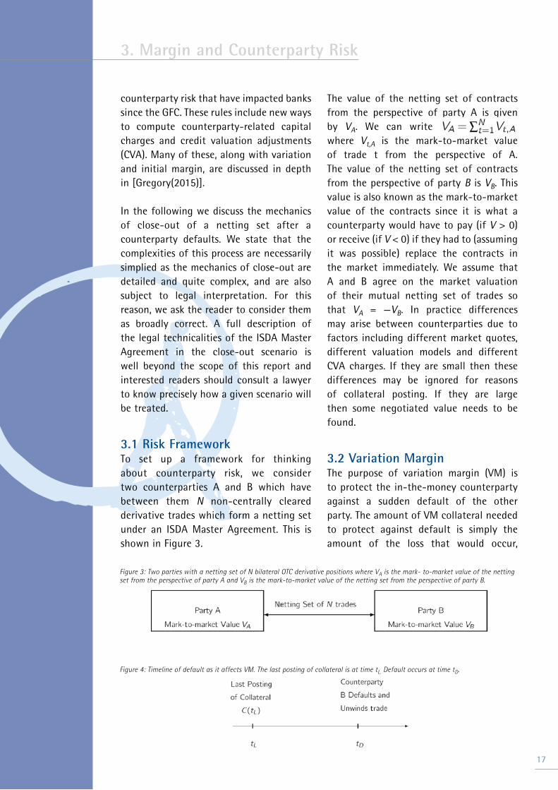
3.1 Risk FrameworkTo set up a framework for thinking about counterparty risk, we consider two counterparties A and B which have between them N non-centrally cleared derivative trades which form a netting set under an ISDA Master Agreement. This is shown in Figure 3.

The value of the netting set of contracts from the perspective of party A is given by VA. We can write where Vt,A is the mark-to-market value of trade t from the perspective of A. The value of the netting set of contracts from the perspective of party B is VB. This value is also known as the mark-to-market value of the contracts since it is what a counterparty would have to pay (if V > 0) or receive (if V < 0) if they had to (assuming it was possible) replace the contracts in the market immediately. We assume that A and B agree on the market valuation of their mutual netting set of trades so that VA = —VB. In practice differences may arise between counterparties due to factors including different market quotes, different valuation models and different CVA charges. If they are small then these differences may be ignored for reasons of collateral posting. If they are large then some negotiated value needs to be found.

3.2 Variation MarginThe purpose of variation margin (VM) is to protect the in-the-money counterparty against a sudden default of the other party. The amount of VM collateral needed to protect against default is simply the amount of the loss that would occur,

17


Figure 3: Two parties with a netting set of N bilateral OTC derivative positions where VA is the mark- to-market value of the netting set from the perspective of party A and VB is the mark-to-market value of the netting set from the perspective of party B.

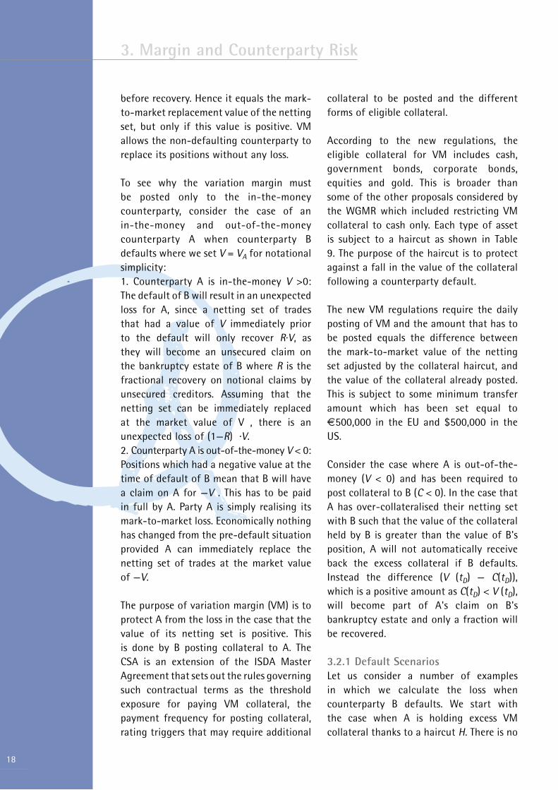
Figure 4: Timeline of default as it affects VM. The last posting of collateral is at time tL. Default occurs at time tD.

18

before recovery. Hence it equals the mark-to-market replacement value of the netting set, but only if this value is positive. VM allows the non-defaulting counterparty to replace its positions without any loss.

To see why the variation margin must be posted only to the in-the-money counterparty, consider the case of an in-the-money and out-of-the-money counterparty A when counterparty B defaults where we set V = VA for notational simplicity:1. Counterparty A is in-the-money V >0:The default of B will result in an unexpected loss for A, since a netting set of trades that had a value of V immediately prior to the default will only recover R.V, as they will become an unsecured claim on the bankruptcy estate of B where R is the fractional recovery on notional claims by unsecured creditors. Assuming that the netting set can be immediately replaced at the market value of V , there is an unexpected loss of (1—R) .V.2. Counterparty A is out-of-the-money V < 0:Positions which had a negative value at the time of default of B mean that B will have a claim on A for —V . This has to be paid in full by A. Party A is simply realising its mark-to-market loss. Economically nothing has changed from the pre-default situation provided A can immediately replace the netting set of trades at the market value of —V.

The purpose of variation margin (VM) is to protect A from the loss in the case that thevalue of its netting set is positive. This is done by B posting collateral to A. The CSA is an extension of the ISDA Master Agreement that sets out the rules governing such contractual terms as the threshold exposure for paying VM collateral, the payment frequency for posting collateral, rating triggers that may require additional

collateral to be posted and the different forms of eligible collateral.

According to the new regulations, the eligible collateral for VM includes cash, government bonds, corporate bonds, equities and gold. This is broader than some of the other proposals considered by the WGMR which included restricting VM collateral to cash only. Each type of asset is subject to a haircut as shown in Table 9. The purpose of the haircut is to protect against a fall in the value of the collateral following a counterparty default.

The new VM regulations require the daily posting of VM and the amount that has to be posted equals the difference between the mark-to-market value of the netting set adjusted by the collateral haircut, and the value of the collateral already posted. This is subject to some minimum transfer amount which has been set equal to $500,000 in the EU and $500,000 in the US.

Consider the case where A is out-of-the-money (V < 0) and has been required to post collateral to B (C < 0). In the case that A has over-collateralised their netting set with B such that the value of the collateral held by B is greater than the value of B's position, A will not automatically receive back the excess collateral if B defaults. Instead the difference (V (tD) — C(tD)), which is a positive amount as C(tD) < V (tD),will become part of A's claim on B's bankruptcy estate and only a fraction will be recovered.

3.2.1 Default ScenariosLet us consider a number of examples in which we calculate the loss when counterparty B defaults. We start with the case when A is holding excess VM collateral thanks to a haircut H. There is no


IM collateral being held in these examples. It is only VM, which is not segregated such that in the event of B's default, any collateral that is held by B will become mixed in with B's estate and so will have to be claimed back by A. As ISDA claims are senior unsecured, they will obtain the corresponding recovery rate.

Example 1: The mark-to-market value to A of the netting set of trades between A and B is $320m, and due to a haircut, the amount of VM held by A is worth $335m. B suddenly defaults. A and B close out the netting set for $320m. A sells collateral worth $320m which is then used to enter into new replacement trades by transacting with other counterparties. The excess VM collateral of $(335—320) = $15m is returned from A to B. A has no loss.

Now consider the same example but with A holding insufficient VM collateral.

Example 2: The amount of VM held by A is only worth $305m. B suddenly defaults. A and B close out the netting set for $320m. A sells VM collateral worth $305m. However they need another $15m to replace the trades. A makes a claim for $15m on B, of which only 40% can be recovered. The loss to A is $(1—0.40)15= $9m.

Now consider an example in which V is negative and B defaults. This example is different because A does not hold any variation margin and would receive money if it were to enter into the replacement OTC derivative. As we will see, A loses because it has over-collateralised its trade with B.

Example 3: The value to A of the netting set of trades between A and B is -$120m.

Due to a haircut, B holds VM collateral worth $130m. B suddenly defaults. A terminates the trade and wishes to replace it at -$120m, receiving $120m. B keeps enough of A's VM collateral to cover its claim. A must then make a claim on A for the excess VM collateral worth e10m in order to replace its position. Because this is VM collateral that has not been segregated, it involves a claim on B's bankruptcy estate. Assuming a 40% recovery rate, this is a loss of $6m.

We do not consider the case when the amount of collateral posted by A to B is insufficient to cover A's claim. In this case A simply pays the difference and neither A or B incur a loss. A loss only occurs to A if it has insufficient collateral or it has posted too much VM collateral. We can therefore generalise the loss to A using the following formula

If A has posted collateral to B then CA < 0.It is simple enough to confirm this formula by considering each of the above examples. We note that between tL and tD the value of either the trade or the collateral can change.

To summarise, VM protects the non-defaulting counterparty from incurring a loss provided the VM collateral held is sufficient, and any collateral posted is not excessive. In the following section we examine what happens if the value of the netting set V and C, the value of the collateral held, change between the last collateral posting and the close-out of the derivative trades.


19

20

3.3 Initial MarginInitial margin (IM) is intended to protect the non-defaulting counterparty against the loss that occurs if the cost of replacing (or closing out) the netting set of trades exceeds the amount of variation margin (VM) held. This can happen if the mark-to-market value of the netting set to the non-defaulting counterparty has increased since the last variation margin payment was made. Such a scenario is most likely to occur if counterparties are unable to replace their positions quickly due to a drop in market liquidity, thereby providing more time for market movements, or if there are very sudden price movements in the period following the default.

A full timeline of the events leading to a need for initial margin could be fairly complex. Consider this from the perspective of an in-the-money counterparty A. Assume that the last posting of collateral was at time tL so that the amount of VM collateral held is C(tL). Another VM posting is now due on date tC. A calculates the mark to market value of the netting set to give V (tC). The value of V (tC) is then communicated to counterparty B on the following day. Provided there is no dispute regarding this amount, and assuming that V (tC) — C(tC) > θ, where is the minimum transfer amount19, collateral equal in value to V (tC) — C(tC) is then posted from B to A. This may not happen until the following day.

Suppose B is in financial difficulty, but not yet in default. In this case, the collateral may not be paid immediately as B may wish to hold on to its liquid assets in an attempt to stave off default. B may do this by contesting the valuation and this dispute could last days, and potentially longer. There is also a question of whether other contractual payments such as swap

fixed or floating payments would be made during this period, and also whether collateral held by A would be returned. Eventually B defaults, but the time delay between the last posting of collateral at tL and the default time could easily add up to a week or more.

Now we consider the situation at time tD immediately after B announces that it is entering bankruptcy proceedings. In some jurisdictions, an immediate stay on the actions of creditors comes into effect immediately after a bankruptcy filing. Normally this would block an immediate close-out and possibly make it subject to the decision of the bankruptcy court. However some bankruptcy codes, most notably in the US, have carved out a `safe harbour' exception for OTC derivatives20 meaning that they are excluded from the stay and so trades may be closed out immediately.

Market volatility is likely to increase in the aftermath of the bankruptcy of B and this can cause the value of the netting set of trades to become more volatile than usual. If the value of the netting set increases, then it will cost A more to replace the defaulted trades than before, and given that the increase has not been collateralised with VM, A has an increased loss. If the value of the netting set falls then A will use the VM collateral to cover the replacement cost and will suffer no loss.

Note that in some actual cases one party has intentionally delayed the process of closing-out the netting set under the safe harbour provision.21 One possible motive for doing this may be if he or she believes that the value of the netting set is moving in his or her favour. This is generally not permitted and if such tactics become


19 - $500,000 in US and e500,000 in EU.20 - See Page 36 of [Murphy(2013)].21 - See for example http://www.cadwalader.com/resources/clients-friends-memos/lehman-bankruptcy-court-holds-isda-swap-counterparty-in-violation-of-automatic-stay-counterparty-seeks-modification.

apparent, they will typically be ruled against by the bankruptcy court.

Figure 5 depicts the timing delay that leads to the need for initial margin. As before we have a trade between parties A and B where the last posting of VM was at time tL. Counterparty B defaults at time tD. We assume that following B's default, a lack of liquidity and other restrictions mean that party A can then only replace the positions at a later time tU and at a price VA(tU). The time between the last posting of collateral tL and replacement of the positions is called the margin period of risk (MPR).

3.3.1 Post-Default Close-Out Scenarios with VM onlyTo understand the mechanics of VM when there is a delayed close-out, and to quantify the loss that the initial margin amount is intended to cover, we consider a series of examples, all from the perspective of the non-defaulting counterparty A. In the first, we consider what happens if A is in-the-money and B defaults.

Example 1: Party A has a netting set of derivatives with B worth e135m. Due to a haircut, B has posted VM to A with a value of e138m. B defaults and the VM

collateral is sold immediately. Market events lead to a delay in agreeing a close-out price until six days later. On this date the cost of replacing the defaulted trades is agreed to be e145m. But A only has collateral worth e138m, so A claims e7m from B. Assuming a 40% recovery they get e2.8m and lose Loss to A = (1—R) Max[VA(tU)—CA(tU), 0] = 0,6 . Max[145—138, 0] = e4.2m.

In this example, A was partly protected by the over-collateralisation of the VM. Now we consider a scenario in which party A is out-of-the-money. This scenario is different because A has posted VM collateral to B and this must be accounted for when considering any extra cost incurred in replacing the netting set.

Example 2: Party A has a netting set of derivatives with B with a mark-to-market value of -e135m. It is holding no collateral but has posted VM to B with a value of e145m. B defaults and sells the collateral immediately for cash. A is unable to replace its trades until six days later by which time the netting set has increased in value to -e120m. A closes out the trade with B at this value. The e25m of excess collateral becomes the


21

Figure 5: Timeline of default as it affects IM. The last posting of collateral is at time tL. Collateral disputes delay subsequent collateral postings between tL and the time of default tD of counterparty B. Market disruptions mean that the netting set is not closed out until time tU. The time tU —tL is called the margin period of risk (MPR).

22

subject of an unsecured claim on B from A. Assuming a 40% recovery, A loses e15m. Once again the loss formula is given by Loss to A = (1—R) Max[VA(tU)—CA(tU), 0] = 0.60 . Max[—120—(—145), 0] = e15m.

Finally we consider an example in which the sign of the value of the netting set flips between default and close-out.

Example 3: Party A has a netting set of derivatives with B worth -e15m. A has posted VM to B with a value of e18m. B defaults. Market events lead to a delay in agreeing a close-out price until six days later. On this date the cost of replacing the defaulted trades has become +e10m. B no longer has a claim on A but A has a claim on B of e10m. It also requires e18m of collateral to be repaid so A has a total claim of e28m. With a recovery rate of 40%, A loses Loss to A = (1—R) Max[VA(tU)—CA(tU), 0] = 0.60 . Max[10—(—18), 0] = e16.8m.

What is common to all of these scenarios is an increase in the value of the trade over the value of the collateral at the default time from the perspective of the non-defaulting counterparty. The loss formula is the same whether VA > 0 or VA < 0. The IM is set so that it can cover this loss to a high confidence. We see from this formula that IM will be needed by either of the twocounterparties to a netting set, although only the non-defaulting party is permitted to use it. The loss for party A if B defaults is given by IM Loss to A = (1—RB) Max[VA(tU)—CA(tU), 0] and for party B if A defaults is IM Loss to B = (1—RA) Max[—VA(tU)—CA(tU), 0].

where RA and RB are the respective recovery rates of party A and party B following their default. These loss amounts depend on the change in the value of both the netting set

and the collateral between tL and tU. If we are being conservative then we can assume that RA = RB = 0. In both cases we know that CA(tL) = V (tL) / (1—H) at the last time of collateral posting tL Unless in cash, the value of this collateral will almost change between tLand close-out time tU.

3.3.2 Default Scenarios with IMNow reconsider an examples from the perspective of the non-defaulting counterparty A. In this case both parties have posted initial margin.

Example 1: Party A has a netting set of derivatives with B worth e135m. Due to a haircut, B has posted VM to A with a value of e138m. A and B have both calculated and exchanged IM worth $10m. B defaults and A is unable to replace the trades until six days later. On this date the cost of replacing the defaulted trades is agreed to be e145m. Also, A has VM collateral now worth e138m. The cost to A of closing out the trades has led to a loss of e145—e138 =e7m. Party A simply uses the $10m of IM that B deposited to cover this loss. The remaining e3m is returned to B. A receives back his $10m in IM collateral from B as it has been segregated.

The loss is now completely covered by the IM. If the loss had exceeded the IM then A would have had a claim on the bankruptcy estate of B, and so would have incurred a loss on the unrecovered fraction of this amount.

3.4 The Distribution of LossesThe risk covered by IM is a future loss conditional on an increase in the value of the netting set (or a decline in the value of the collateral, or both) following the default of the other counterparty. So any


attempt to model the loss amount for party A has to simulate the change in the value of the netting set ∆VA from time tL to tU and so needs to reflect the market environment following the default of a major derivatives dealer. Model calibration presents a problem as we do not have many examples in which large derivatives counterparties have defaulted, allowing usto empirically estimate the typical market adjustment.

A full model-based calculation of IM would need to take into account the volatility of the value of the position, the impact of the default of the counterparty on market liquidity, and the impact of the default on any tendency for the value of the position to increase before it can be re-established. If we wish to take into account the effect of collateral, we would then need to add that to the netting set portfolio and to take into account the effect of any correlations.

The output of the model needs to be a distribution of the loss due to future value changes of the netting set (including collateral) between time tL and time tU. We therefore define ∆V = V(tU)—C(tU) where C(tU) is the value at time tU of the collateral that has been posted. There will be two values of IM, one for counterparty A and one for counterparty B. These can be written as

IM Loss to A = Max[VA(tU)—CA(tU). 0]

IM Losst to B = Max[CA(tU)—VA(tU). 0].

For this reason, whether V refers to VA or VB depends on which counterparty we are considering. We also define ρ(∆V) to be the probability density function of ∆V. We note that this distribution of losses is almost certainly not symmetric about ∆V = 0. Its shape is driven by the pay-off

of the derivative trades in the netting set portfolio and the form of the distribution assumed for the underlying risk factors.

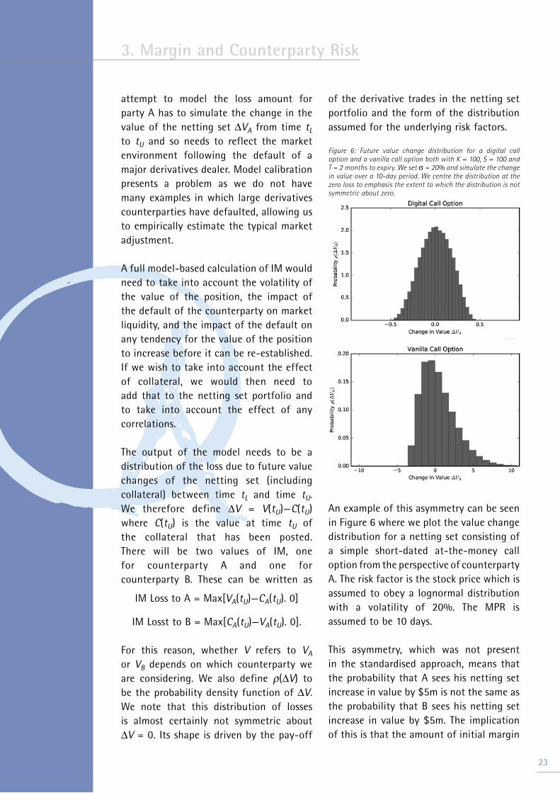
Figure 6: Future value change distribution for a digital call option and a vanilla call option both with K = 100, S = 100 and T = 2 months to expiry. We set σ = 20% and simulate the change in value over a 10-day period. We centre the distribution at the zero loss to emphasis the extent to which the distribution is not symmetric about zero.

An example of this asymmetry can be seen in Figure 6 where we plot the value changedistribution for a netting set consisting of a simple short-dated at-the-money call option from the perspective of counterparty A. The risk factor is the stock price which is assumed to obey a lognormal distribution with a volatility of 20%. The MPR is assumed to be 10 days.

This asymmetry, which was not present in the standardised approach, means that the probability that A sees his netting set increase in value by $5m is not the same as the probability that B sees his netting set increase in value by $5m. The implication of this is that the amount of initial margin


23

24

that A must post to B is not the same as the amount that B must post to A. This adds a certain amount of additional negotiation to the IM posting as it means that both parties must be able to agree on two values rather than just one.


Following the Pittsburgh declaration, the body charged with drawing up the detailed regulations for the non-cleared derivatives market has been the Basel Committee on Banking Supervision (BCBS) and the Board of the International Organization of Securities Commissions (IOSCO). In this section we provide an overview of the new VM and IM regulations put forward by theWGMR. These can be found in the March 2015 version of Margin requirements for non-centrally cleared derivatives22.

4.1 Variation Margin RegulationsWhile VM has been an aspect of OTC derivatives markets since their inception, and is documented by the ISDA CSA, it has not always been universally applied. Under the new regulations the scope of market participants who are subject to VM has been defined explicitly. One of the key principals of the new regulations states that all financial firms and systemically important non-financial entities (`covered entities') that engage in non-centrally cleared derivatives must exchange initial and variation margin as appropriate to the counterparty risks posed by such transactions'. The range of covered entities includes financial firms and those non-financial firms deemed to be systemically important. However, it does not include central banks, development banks and sovereign issuers.

The new regulations note that VM should be posted with `sufficient frequency (e.g. daily)'. This is subject to a minimum transfer amount of e500,000 in the EU and $500,000 in US. The size of the VM that needs to be held is the market value of the netting set of derivatives (which will be positive for the party receiving VM). As some of the products in the netting set may be exotic or illiquid,

determination of their market value may be partly subjective and subjectto dispute between both parties. For this reason, the BCBS/IOSCO has insisted that `robust' dispute resolution procedures need to be put in place before such trades are executed.

The form of collateral permitted for VM is quite broad as we discuss below. There are no restrictions on what the party receiving the collateral can do with it. It does not need to be segregated and can be rehypothecated. Clearly, if the counterparty defaults and the non-defaulting counterparty is in-the-money but has rehypothecated the collateral it has received, it is very much in their interest to make sure that they can have this collateral returned. Unfortunately this mixing of assets means that a non-defaulting counterparty that has posted variation margin worth more than the value of the netting set will not have its excess collateral returned automatically following a default. Instead they will need to enter a claim in the bankruptcy process.

In terms of liquidity, the posting of VM does transfer liquidity from the poster to the receiver and so the poster loses use of the collateral. It is a gain in liquidity for the receiver of the collateral. Therefore, the effect on the overall liquidity of the market is unchanged. This is one feature in which VM is very different from IM.

A timetable for the implementation of the new VM regulations is shown in Table 5. This shows that it is expected that there will be a universal application of VM after early 2017. For large entities which have a monthly notional of non-centrally cleared derivatives in excess of e3 trillion, the range of contracts subject to the new rules are those transacted after 1 September

4. The Regulatory Framework

2522 - See http://www.bis.org/bcbs/publ/d317:pdf

26

2016. For the remaining parties it only applies to contracts transacted after 1 March 2017.

4.2 Initial Margin RegulationsAssuming that the default of a financial institution is sudden and unpredictable, the loss event which IM is intended to cover can potentially cause either of the two parties to incur a loss. However, IM only protects the non-defaulting party. For this reason, the regulations around IM differ in a number of fundamental ways from those governing variation margin.

In terms of product coverage, the new IM requirements are very broad as they apply to all non-centrally cleared derivatives, except physically settled currency forwards and swaps. For cross-currency swaps they do not apply to the fixed physically settled FX transactions associated with the exchange of principal.

The WGMR has stated as a principle that IM should be based on a `defaulter pays' approach. Since the loss that IM covers can impact either party, the regulations require an exchange of margin by both parties. In order that the margin posted by the defaulting counterparty is immediately available to the non-defaulting counterparty at the time of default, and additionally that the margin posted by the non-defaulting counterparty is returned. Because of this requirement, the IM cannot be reused, repledged or rehypothecated (except for very specific hedging purposes described in the WGMR framework document). It is key that the margin amounts are held in a ring-fenced segregated account. This suggests the use of a third-party custodian account.

The overall result is that summed across the financial system, the amount of IM collateral posted will greatly exceed the likely realised losses that might occur following a counterparty default. Consider, for example, a world of N counterparties,


Table 5: The implementation timetable for Variation Margin. The regulations are expected to be fully implemented by 1 March 2017.

Implementation Date Who pays Variation Margin and When

1 September 2016 After this date any covered entity with monthly notional non-centrally cleared in excess of e3 trillion across March, April and May 2016 will be required to exchange VM for contracts traded after 1 September 2016

1 March 2017 After this date all covered entities will be required to exchange VM

Figure 7: Two parties A and B depositing IM with a third-party custodian. The amounts IMA and IMB can be different and are held in segregated accounts.

and suppose they all face identical and symmetric risks resulting in an initial margin for each counterparty equal to G. In this case the total amount of initial margin posted will be N(N—1)G. We would not expect secondary defaults due to the use of VM and IM. However, if one counterparty defaults, the total losses will, with high confidence, be less than (N—1)G. So the system is effectively putting aside N times as much collateral as is needed to protect against a default.

Collateral that has been provided as initial margin from a customer (buy-side financial firm or non-financial company) can be rehypothecated for the purpose of hedging the derivative positions of the receiver of the collateral only if permission has been given by the provider. The collateral must also be held in a form that protects the rights of the customer. If the customer has agreed to allow rehypothecation, then they have to be informed of this and how much has been rehypothecated.

As with the VM, the form of collateral used for IM must be accessible when needed and be provided in a form that can be `liquidated rapidly and at a predictable price even in a time of financial stress'. In order to mitigate this loss of liquidity, the rules allow a fairly broad range of assets to be used, albeit subject to a haircut. These haircuts are the same as those used for VM.

To restrict the imposition of IM to counterparties with large derivatives exposures, regulators have imposed an IM threshold. This states that no IM has to be posted until the amount of IM exceeds e50m. Beyond this threshold, the amount of collateral to be posted is the differencebetween the IM amount and the threshold. To prevent companies from creating new entities in a group structure in order to reuse the threshold, the threshold can only be applied on a consolidated group basis.

The timetable for the introduction of IM is given in Table 6. There is a gradual ramp-up phase in terms of counterparty size, as determined by the monthly notional of non-centrally cleared OTC derivatives traded by that party. It is envisaged that the IM arrangements will be fully operational by the end of August 2020.

4.3 Collateral HaircutsBoth VM and IM require the posting of collateral. Because this collateral is needed to protect against losses in the scenario in which one counterparty defaults, it is essential that the collateral is able to hold its value in times of financial stress. One concern is that the collateral value could be correlated to the event of a bank default and this, according to the regulations, should be avoided.


27

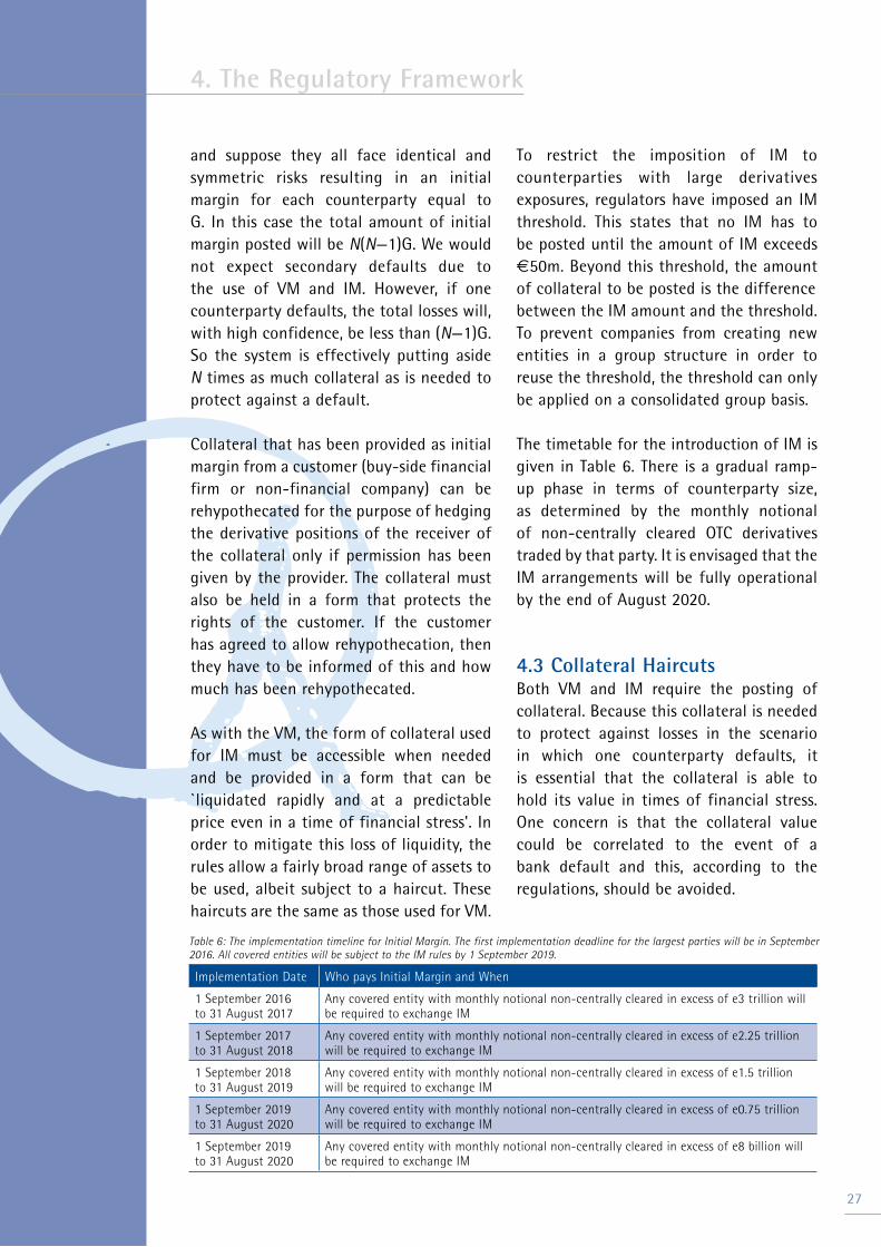
Table 6: The implementation timeline for Initial Margin. The first implementation deadline for the largest parties will be in September 2016. All covered entities will be subject to the IM rules by 1 September 2019.

Implementation Date Who pays Initial Margin and When

1 September 2016to 31 August 2017

Any covered entity with monthly notional non-centrally cleared in excess of e3 trillion will be required to exchange IM

1 September 2017 to 31 August 2018

Any covered entity with monthly notional non-centrally cleared in excess of e2.25 trillion will be required to exchange IM






Any covered entity with monthly notional non-centrally cleared in excess of e8 billion will be required to exchange IM

28

One way to reduce this risk would be to limit the range of collateral to only the safest form of assets, e.g. cash or short-term Treasury bills. However, this could have a negative impact on market liquidity, especially as this IM collateral cannot be re-used or re-hypothecated. For this reason, the WGMR has widened the range of eligible collateral to include cash, high quality government bonds and central bank securities, high-quality corporate bonds, high-quality covered bonds, equities in major stock indices and gold.

To adjust for the riskiness of these assets, a table of haircuts has been provided and this is shown in Figure 7. The eligible collateral can also be in any currency, and this explains the last row of the haircut table which imposes an 8% haircut on collateral if it is denominated in a different currency from that of the netting set derivatives.

Because of the limits on re-use and re-hypothecation, one of the major concern across banks is the impact of initial margin on market liquidity. An analysis of the expected liquidity impact of IM has been performed by the WGMR. Known as the Quantitative Impact Study, this was carried

during 2012 and 2013 and shows23 that if a threshold for IM of e50m ($65m in US) is used, the amount of IM required would be around e558 billion. This is a substantial amount of collateral, especially as it cannot be rehypothecated. A 2014 report by the European Central Bank (ECB) estimates24 that the overall supply of high quality assets at a global level is around e41 trillion. If we restrict collateral to those eligible for CCPs, the number drops to a range of between e2 and e14 trillion. And if we just consider margin eligible for initial margin, we get e5 to e28 trillion. This seems to be well in excess of the e558 billion mentioned above. But we should be aware that this is in the context of additional liquidity requirements that are being applied to banks such as the Liquidity Coverage Ratio25 and Net Stable Funding Ratio26. So while sufficient collateral does exist, demand for high-quality collateral is growing.

4.4 Comparison of US and European RegulationsWe have already mentioned that the WGMR framework is to establish minimum global standards that legislators can then translate into law. In the US, the rules have


23 - See http://www.bis.org/publ/bcbs242:pdf24 - See https://www.ecb.europa.eu/pub/pdf/other/cea201407en.pdf?c5856909bbcb7b0ed884be5b281ddc24.25 - See http://www.bis.org/publ/bcbs238:pdf26 - See http://www.bis.org/publ/bcbs271:pdf

Table 7: The schedule of standardised haircuts as they apply to derivatives for which the asset class is the primary one for that derivative. See Appendix B of www:bis:org/publ/bcbs261:pdf

Asset Class Collateral Haircut (% of value)

Cash in same currency High quality government bonds and central central bank securities

0

Under 1 year 0.5

1-5 years 2

Over 5 years 4

High quality corporate/covered bonds

Under 1 year 1

1-5 years 4

Over 5 years 8

Equities in major stock indices 15

Gold 15

Currency mismatch 8


29

been set by the CFTC27 and in Europe they are being set by ESMA, the EBA, and EIOPA. We now wish to discuss the main regional differences between the US and Europe.

In the US, the new VM and IM rules apply to any `covered swap entity' (CSE) which is a CFTC-registered swap dealer or major swap participant. It exempts those parties that deal with less than $8 billion of notional a year and those who are declared to be non-financial end users. VM will be required for all financial end users and for swap entities who trade with CSEs. A CSE must post or collect IM within one business day after a swap is executed subject to a minimum transfer amount of $500,000 and a threshold value for IM of $65m. The daily posting of VM collateral is also required and has the same minimum transfer amount. The IM amount can be calculated using a model or use the standard table of add-ons shown in Table 9. The US rules recognise an additional number of asset categories that may be used in an initial margin model with the set of risk categories and these include agriculture, energy, metals, and other commodities. The US law also exempts certain products from the margining requirement. It also broadens the range of the calibration period to 1-5 years. It also requires collateral to be segregated at third-party custodians.

The EU rules have fewer changes with respect to the WGMR framework. The covered entities are financial counterparties (FC), non-financial counterparties (NFCs) as classified under EMIR, and those above the EMIR clearing threshold (NFC+). While any covered entity must exchange VM, only those with an aggregate month-end notional amount of non-centrally cleared derivatives of over e8 billion have to exchange IM. All OTC derivatives that have not been cleared by a CCP are subject to the new margin rules. The minimum transfer amount under EMIR is e500,000. The threshold for posting IM is e50m. A summary of the differences can be found in Table 8.

27 - See Federal Register at http://www.cftc.gov/idc/groups/public/@lrfederalregister/documents/file/2015-32320a.pdf.

Table 8: A list of the main differences between US and EU implementations of their regulations on margin for non-cleared OTC derivatives.

Regulation EU Treatment US Treatment

Covered Entities Financial and Non-Financial Exempts Non-Financial Entities

Minimum Transfer Amount e500,000 $500,000

IM Threshold e50m $65m

Covered Transactions Exempts options on certain securities

Eligible Collateral An 8% charge when currencies of collateral and derivative differs

Requires collateral to be in USDor currency of swap

IM Model Categories 4 in Europe 4+ in US

Calibration Period 3-5 years 1-5 years

IM Segregation US requires segregation at3rd party custodians

30


The IM charge is designed to be a protection against a potential future exposure (PFE) in which the cost of closing out a netting set of trades exceeds the amount of VM held. This potential loss cannot therefore be known either now, or even at the time of the counterparty default. The most we can do is to construct a model which can quantify the possible distribution of lossesand to extract from that a tail risk amount with some defined confidence level.

To achieve its aim, the modelling approach must be conservative such that to some high level of confidence, the amount of posted IM will be sufficient to cover any loss in most scenarios. Equally it must be reasonable. A charge that has been set too high could damage the non-cleared derivatives market. Also, the amount of IM required should be aligned with the risk that it is intended to hedge. If this is not the case then behaviours could develop which would be counter to the objectives of IM.

The WGMR has proposed two approaches for the calculation of IM. The main suggestion is that market participants will calculate IM using an approved but non-specified IM model (Article 1 MRM). This model can be developed by a single counterparty, be a collective effort or can be a third-party model. For those unable to adopt this approach, there is a specifically defined fall-back standardised approach (Article 1 SMI). We now describe these in turn beginning with the standardised approach.

5.1 The Standardised Approach (Article 1 SMI)The WGMR has introduced a standardised approach to calculating the IM which avoids the need for an internal IM model.

It is based on the schedule of IM àdd-ons' shown in Table 9. Each of the N trades in the netting set must be assigned to one of the asset class categories in this table. This assignment must be based on its primary risk factor, which must be clearly identifiable. If it is not possible to identify the primary risk factor then it is calculated using the highest IM weight within the relevant category. Some of the fixed income products have a maturity-dependent add-on. This means that the IM add-on would change as time passes and it moves from a longer maturity bucket to a shorter one.

The IM calculation procedure is straightforward and can be broken down into two stages. Stage one is the calculation of the Gross Initial Margin which takes into account the IM of each trade. Stage two is the calculation of the Net Initial Margin (NIM) which is the amount of IM that has to be posted. The calculation attempts to take into account the diversification of the netting set. We now examine how this is done in more detail.

The add-on weight, corresponding to this asset class, which we denote with Mt is multiplied by the notional of the derivative Ft (which is always positive) and the process repeated for all contracts. Hence for a netting set of N trades we calculate the Gross Initial Margin (GIM) as follows

At this stage netting is only permitted for contracts that are fungible, i.e. they have identical features and only differ in their face values. In this case Ft will be the net notional of those contracts.

The next stage of the calculation allows for netting across positions within each asset

5. Regulations for Calculating Initial Margin

31

32

type category of which there are four: (i) interest rates and foreign exchange, (ii) credit, (iii) equities and (iv) commodities. The netting formula is

NIM = (0.4 + 0.6 x NGR) x GIM

where the NGR is the ratio of the net current replacement cost of the netting set to the gross current replacement cost of the netting set. It is given by

where Vt is the replacement value of derivatives positions t denoted by Vt. If the value of all of the positions is positive (or negative) then the NGR equals one and the net IM equals the gross IM. If the position replacement values net out to zero then the NGR equals zero and the net IM reduces to 40% of the GIM. This is the effective floor on the NGR.

The calculation of the Net Initial Margin does not take into account the direction of the positions, i.e. it is unchanged if we set Vt = —Vt . This means that both parties should calculate the same NGR and hence the same value of initial margin. While this simplifies matters, it does implicitly assume that the value change distribution of the netting set is symmetric about zero.

5.2 Discussion of the Standardised ApproachThe main concern we have with the NIM is the way it accounts for diversification through the use of the NGR. To be meaningful, the NGR should capture the net market sensitivity of the netting set. Trades which are hedges for other trades should reduce the NGR and trades which are large and unhedged should increase the NGR. However, instead of using sensitivity, the NGR uses the replacement value of a trade as the basis for the NGR calculation. There is no direct link between the replacement value of a trade and its sensitivity.

To analyse the properties of the official NIM approach, we consider a simple alternativemodel of portfolio sensitivity for interest rate swaps. This model would need to capture the degree of sensitivity of the value of the netting set with respect to market risk factors. We write the value of the N derivative trades within the asset group subdivision of a netting set of trades as follows . The price sensitivity with respect to risk factors St is given by the swap DV01. This is the change in the swap replacement value for a 1bp increase in swap rates. In the case of swaps, we can write the trade t value as Vt(S) where S is the swap rate. The swapvalue sensitivity to a 1bp in swap rates


Table 9: The schedule of standardised IM weights proposed by the WGMR by asset class. For fixed income products the initial margin add-on also depends on the residual maturity. Source: www:bis.org/publ/bcbs261.pdf

Asset Class Subclass Initial Margin Add-On (%)

Credit 0 - 2 year residual maturity 2

2 - 5 year residual maturity 5

5+ year residual maturity 10

Commodity 15

Equity 15

FX and Interest rate

Foreign exchange 6



5+ year residual maturity 4

Other 15

is called the DV01. As the whole IM framework is based on the idea of a 99th percentile move in market rates over a 10-day period, we estimate the 99th percentile of the distribution of 10-day changes in the swap rate. An analysis of USD swap rates over 2005-2010, where the results are in Table 15 shows that the 99th percentile of swap rate changes was close to 50bp for most tenors. This simple model for a netting set of interest rate swaps gives us an alternative NIM measure equal to (1)

To quantify the difference between the official NIM and the Alternative NIM, we randomly generated 1,000 interest rate swap netting sets, each consisting of 50 trades28. For each netting set we calculated the NIM using Equation 3 and compared it to our simple model in Equation 1. The results are shown in Figure 8.

We make two observations. First, there is only a very weak correlation (around 20%) between the price sensitivity of the netting set and the official NIM.

This makes it plain that the NIM is not capturing the diversification of the netting set. Some of this correlation is due to the NIM capturing the swap rate sensitivity of individual positions through the GIM as the add-on depends roughly linearly on the term of each swap. We note that the official NIM is always greater than the Alternative NIM estimate, which has itself been calibrated to the model specification for initial margin, i.e. 99% tail, 10-day risk horizon. This suggests that the standard approach is unduly conservative. Indeed we would recommend that WGMR propose the approach captured by Equation 1. First, it captures the risk that IM is intended to hedge and it takes into account diversification of the netting set. It is also as simple to compute as most swap counterparties would be expected to compute and store the DV01 of each swap trade for their internal risk management.29

Another criticism of the NIM methodology is that it does not treat the risk of optionscorrectly. An option which is out-of-the-money and an option that is in-the-money will have very different risk sensitivities


33

Figure 8: Comparison of the WGMR official calculation of the NIM versus an alternative model-based sensitivity measures. Each point in the scatterplot corresponds to a randomly drawn netting set of 50 swap trades (see text for description of the swap parameters used).

28 - The swap notionals were i.i.d., drawn from a Gaussian distribution with mean zero and a standard deviation of $50m. Each swap maturity was drawn from a uniform distribution out to 10 years and each swap fixed coupon was also drawn from a uniform distribution between 1% and 7%. We assumed a flat market swap curve at 4%.29 - During the course of writing of this report in 2015 the ISDA SIMM model was published and proposed a similar, albeit slightly more complex, modelling framework for IM.

34

which should be accounted for when calculating the NIM. This can be done by delta-weighting the option notionals, where the delta is the sensitivity ratio of the option value to a small change in the price of the underlying. This would be important for major OTC option markets such as interest rate swaptions.

Taken together, these criticisms make it hard to recommend the standardised approach except for those with very simple netting sets of small numbers of non-offsetting trades. This is unfortunate as a more meaningful standardised approach could easily be introduced by allowing the use of first order sensitivities such as swap DV01s and option deltas. It suggests that, intentionally or not, the regulators will push most market participants towards the approved initial margin model framework which we describe next.

5.3 The Approved Initial Margin Model FrameworkThe second IM approach set out in the regulations is to use an approved initial margin model. While the WGMR has refrained from imposing any detailed structure of the model (e.g. distributional assumptions) that must used, they have imposed a framework of requirements which we outline here. This includes the confidence level to be used for IM, the calibration period for the model parameters, and the limits on the scope for risk offsetting across asset classes.

First and foremost, the WGMR has stated that the IM charge must be based on a 99% one-tailed Value-at-Risk (VaR) with a 10-day horizon. The upper tail is chosen rather than the lower tail because the distribution is that of the value of the netting set and a loss scenario occurs when

the value of the netting set increases. The 10-day horizon must be extended if variation margin has not been posted daily, in which case it should be from the last posting date until 10 days after the default. Note that 10-day periods are frequently used in regulatory capital calculations as 10 days is supposed to represent the time needed to exit or hedge positions in the trading book.30

A second requirement is that the initial model must also be rich enough to handle the complexity of the products in the netting set, with the regulations citing examples such as barrier options and `more complex structures'. This is a significant requirement, especially as it is not clear with what accuracy complex derivatives need to be captured by the model. If the required accuracy is high, this may be a problem as full revaluations may be slow to calculate and will require the use of significant computational resources and the associated cost. There is an argument that banks be permitted to use fast, approximate approaches for calculating valuations within an IM model since the need for an accurate price is less important than ensuring that an IM can actually be calculated within a reasonable time frame.

A third requirement in the regulations states that ìnterrelationships between derivatives in distinct asset classes such as equities and commodities are prone to instability' (Page 13, 3.4) and more able to break down in periods of financial stress. Therefore IM models may only account for diversification, hedging or risk offsets within well-defined asset classes. The four separate asset classes are (i) currencies and interest rates, (ii) equities, (iii) credit and (iv) commodities. Inflation swaps can be included in the currencies and interest rates class of products. Importantly, the


30 - See http://www:bis:org/publ/bcbs219:pdf

rules state that the IM model cannot allow netting across these asset classes.31 The total IM is the sum of the IM for each class of assets.

This is an important restriction which can penalise hedging. For example, a book of CDS trades presents an interest rate exposure that may be hedged by a set of interest rate swaps. If the netting will not be able to take this hedge into account, the interest rate risk will then be double counted. This may misalign incentives and is in theory something to be avoided. The practical importance of such a choice may not be important given that most products have one main driving factor - later we will examine this question using the example of a CDS contract which presents interest rate risk. However it does appear to be overly restrictive.

The new regulation state that counterparties need to inform competent authorities if they intend to use an IM model approach and that the use of the model must be approved by that authority in advance. The regulations do not specify the details of the initial margin model, leaving model approval to local regulators. It is also stated that approval from one authority does not automatically allow the model to be used in the jurisdiction of another authority. Within the EU, the model can be developed by one or both of the two counterparties, or by a third party based on methodology endorsed for its use in the EU. If a model has obtained approval, the regulations state that it must also be subject to internal governance requirements that assess the value of the model's output against realised data. The model must also be subject to back-testing, to verify that the VaR predictions are in line with market data.

The regulations are also quite precise about the need to calibrate the model appropriately as we discuss below. It is stated that the calibration should be performed to historical data for a time period of 3 to 5 years and that there should be no weighting of the data in terms of giving greater emphasis to recent market movements. The calibration period is also required to include a period of financial distress. This appears to imply that the calibration period should bracket the period of the 2007-2009 GFC. In our calibration section below, we will examine the impact of different calibration periods on model parameters.

We can summarise the modelling framework as follows:1. The IM amount should be based on a VaR measure at the 99th percentile of the potential future exposure (PFE) distribution of the netting set.2. The time taken to replace the positions, the MPR, is set at 10 days, plus the number of days since the last posting of VM.3. Model parameters can be calibrated to shorter periods (e.g. daily) than the 10-day horizon in the IM and then scaled up to this longer period.4. Each trade must be assigned to one of four asset classes. These are (i) currencies and interest rates, (ii) equities, (iii) credit, and (iv) commodities.5. The IM for each subset of trades must be calculated separately and the results summed to give the overall IM. Hedges between trades in different asset classes are not recognised.6. The PFE distribution should be calibrated to a period of at least three years and not more than five years. This period must include a period of financial distress.7. The calibration time series data should be equally-weighted, i.e. no preference is to be given to more recent events.


3531 - The quote is as follows: Ìnitial margin calculations for derivatives in distinct asset classes must be performed without regard to derivatives in other asset classes' (Page 14, Paragraph 1).

36

8. The model must be recalibrated every six months.

Given these constraints, the main freedom left to IM risk modellers is the choice of dynamics to assume for the various asset classes, plus the precise choice of which valuation models to use for the various derivative securities in the netting set. Once the model dynamics and implementation have been selected, the final challenge is to decide upon how best to calibrate the model and to what exact time period.

In a number of respects, this modelling framework is to be welcomed as it removes a number of burdens from the shoulders of risk modellers. First, attempting to calibrate a model of market price dynamics after the default of a major counterparty is not easy given that we only have one recent data point in the Lehman bankruptcy. The 99% tail probability is intended to combine the stressed nature of the markets after a counterparty default and the level of confidence with which the IM is expected to cover the potential replacement costs.

Considerations regarding the advantages and disadvantages of using a VaR measure versus some other tail risk measure are not left open to the model builders. It may be argued that an expected shortfall measure would be better given that it satisfies the sub-additive requirements of a so-called `coherent risk measure' as discussed in [Artzner 1999], which VaR does not. The counter-argument is that the nature of the value change distributions is expected to be well-behaved, i.e. it will almost certainly be based on risk factors which are assumed to be Gaussian or Gaussian-like such that this weakness of VaR should not be encountered. This can probably be argued for FX, interest rate and equity derivatives.

Issues such as pro-cyclicality are not discussed within the framework, implying that it should not be modelled as a priority. However pro-cyclicality is mainly an issue if the model parameters can change frequently within an economic cycle. However the long calibration period of between 3 and 5 years, the lack of weighting schemes, and the requirement that the calibration period include a period of financial distress, should all make the model parameters fairly insensitive to short periods of low or high market volatility and dampen down any pro-cyclical effects.

The regulations also permit the use of an initial margin model for the calculation of collateral haircuts.32 Our understanding of this is that this would involve treating the collateral as a separate portfolio and calculating its 1st loss percentile. This is fairly straightforward since the collateral will almost surely be exposed to the some or all of the same factors as the netting set. What would be even better than this would be to allow both the collateral and the netting set to be treated as a single portfolio such that correlations between the derivatives and collateral can be quantified. It is not clear that this is permitted within the IM framework.

There are costs associated with an IM model. Not only is there the effort required to make a choice of model and calibration, the implementation an IM system imposes a significant effort. For example, it requires the programming up of the model, the incorporation of the derivative valuation models and the coding up of all of the data plumbing needed for any such system. Even for the largest banks, these implementation costs could be significant.

We suppose that the IM model is run at the end of the day to ensure that all new


32 - BCBS 261 Paragraph 4.3.

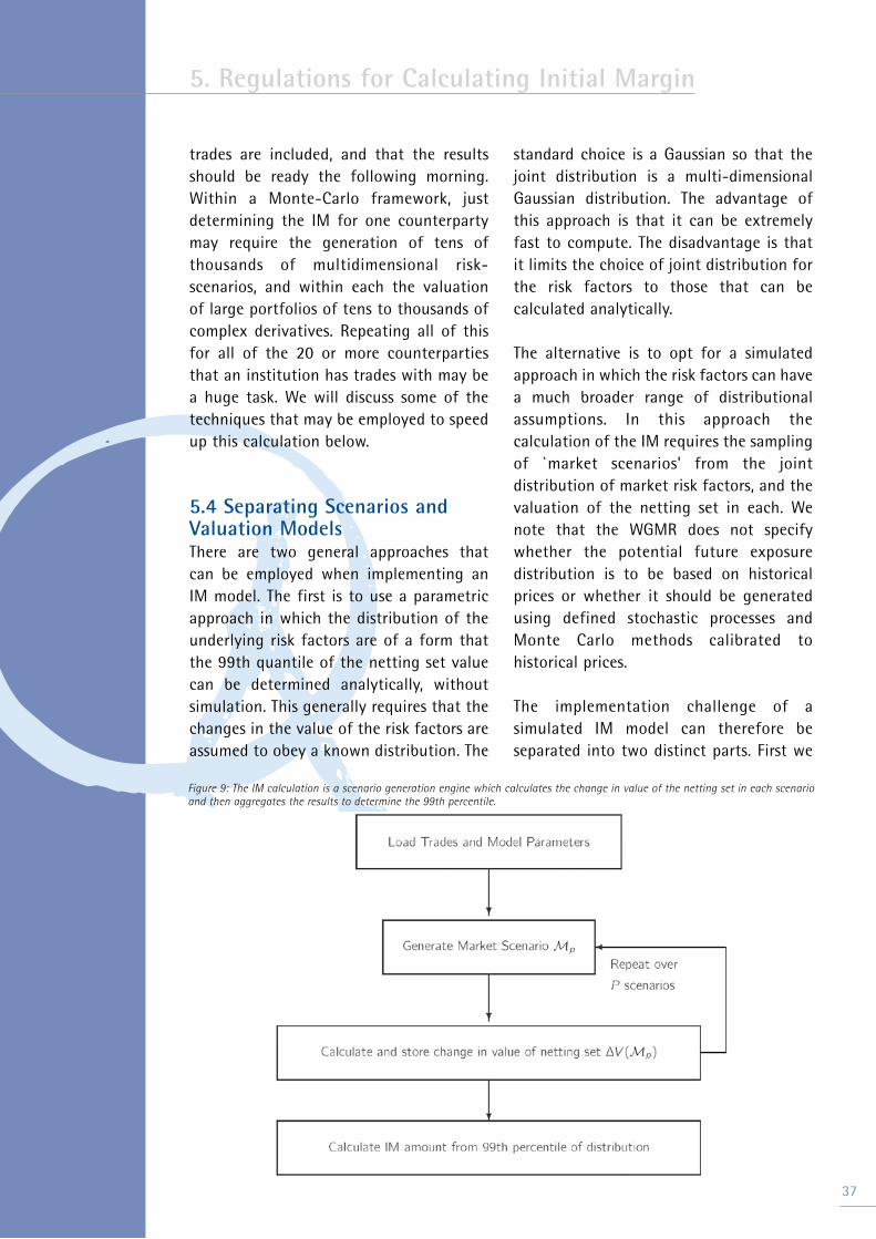
trades are included, and that the results should be ready the following morning. Within a Monte-Carlo framework, just determining the IM for one counterparty may require the generation of tens of thousands of multidimensional risk-scenarios, and within each the valuation of large portfolios of tens to thousands of complex derivatives. Repeating all of this for all of the 20 or more counterparties that an institution has trades with may be a huge task. We will discuss some of the techniques that may be employed to speed up this calculation below.

5.4 Separating Scenarios and Valuation ModelsThere are two general approaches that can be employed when implementing an IM model. The first is to use a parametric approach in which the distribution of the underlying risk factors are of a form that the 99th quantile of the netting set value can be determined analytically, without simulation. This generally requires that the changes in the value of the risk factors are assumed to obey a known distribution. The

standard choice is a Gaussian so that the joint distribution is a multi-dimensional Gaussian distribution. The advantage of this approach is that it can be extremely fast to compute. The disadvantage is that it limits the choice of joint distribution forthe risk factors to those that can be calculated analytically.

The alternative is to opt for a simulated approach in which the risk factors can have a much broader range of distributional assumptions. In this approach the calculation of the IM requires the sampling of `market scenarios' from the joint distribution of market risk factors, and thevaluation of the netting set in each. We note that the WGMR does not specify whether the potential future exposure distribution is to be based on historical prices or whether it should be generated using defined stochastic processes and Monte Carlo methods calibrated to historical prices.

The implementation challenge of a simulated IM model can therefore be separated into two distinct parts. First we


37

Figure 9: The IM calculation is a scenario generation engine which calculates the change in value of the netting set in each scenario and then aggregates the results to determine the 99th percentile.

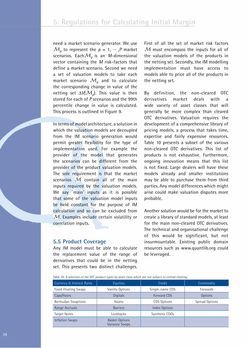
38

need a market scenario generator. We use

p to represent the p = 1, … ,P market scenarios. Each p is an M-dimensional vector containing the M risk-factors that define a market scenario. Second we need a set of valuation models to take each market scenario p and to calculate the corresponding change in value of the netting set ∆V( p). This value is then stored for each of P scenarios and the 99th percentile change in value is calculated. This process is outlined in Figure 9.

In terms of model architecture, a solution in which the valuation models are decoupled from the IM scenario generation would permit greater flexibility for the type of implementation used. For example the provider of the model that generates the scenarios can be different from the provider of the product valuation models. The sole requirement is that the market scenarios contain all of the main inputs required by the valuation models. We say `main' inputs as it is possible that some of the valuation model inputs be held constant for the purpose of IM calculation and so can be excluded from

. Examples include certain volatility or correlation inputs.

5.5 Product CoverageAny IM model must be able to calculate the replacement value of the range of derivatives that could be in the netting set. This presents two distinct challenges.

First of all the set of market risk factors must encompass the inputs for all of

the valuation models of the products in the netting set. Secondly, the IM modelling implementation must have access to models able to price all of the products in the netting set.

By definition, the non-cleared OTC derivatives market deals with a wide variety of asset classes that will generally be more complex than cleared OTC derivatives. Valuation requires the development of a comprehensive library of pricing models, a process that takes time, expertise and fairly expensive resources. Table 10 presents a subset of the various non-cleared OTC derivatives. This list of products is not exhaustive. Furthermore, ongoing innovation means that this list is not fixed. Large dealers will have these models already and smaller institutions may be able to purchase them from third parties. Any model differences which might arise could make valuation disputes more probable.

Another solution would be for the market to create a library of standard models, at least for the main non-cleared OTC derivatives. The technical and organisational challenge of this would be significant, but not insurmountable. Existing public domain resources such as www.quantlib.org could be leveraged.


Table 10: A selection of the OTC product types by asset class which are not subject to central clearing.

Currency & Interest Rates Equities Credit Commodity

Fixed-Floating Swaps Vanilla Options Single-name CDS Forwards

Caps/Floors Digitals Forward CDS Options

Bermudan Swaptions Asians CDS Options Spread Options

Range Accruals Barriers Index Options

Target Notes Lookbacks Synthetic CDOs

Inflation Swaps Basket OptionsVariance Swaps

The valuation models for the range of products in a netting set can range from simple analytical schemes which can compute a trade value in milliseconds to complex multi-factor Monte-Carlo schemes which may take several seconds to value. Because of this, an IM frameworkbased on full revaluation of the netting set across a high number of future scenarios within several hours may be a significant challenge.

One shortcut is to accept that a valuation model needed for calculating IM does not require the same degree of accuracy as a valuation model needed for marking-to-market accounting.

Scenario generation is the outer loop of the whole IM calculation. The brute-force approach is to throw sufficient computing power at the problem to ensure that IM can be calculated within the required time. The feasibility of this depends on the implementation of the scenario generation,and favours Monte Carlo-based approaches. However the only way to significantly reduce the computation time would be to create 99% stressed scenarios using some analytical approach. This would almost surely require simpler modelling assumptions but these may be acceptable for IM purposes. For IM it is perhaps more important that trades are valued accurately than scenarios are sampled in a specific way.

A third approach is to reduce computation time would be to approximate the change in the derivative value using perturbatory techniques, discussed later. Finally, these choices are not mutually exclusive and some combination of all three may be used.

5.6 Market Risk FactorsIn order to value the netting set in each market scenario, the set of risk factors must encompass all of the market observables that would be used to value all of the instruments in a netting set. To indicate the breadth of such factors, a selection is shown in Table 11. We must be careful to distinguish between the real-world

measure and the risk-neutral pricing measure . The generation of the market scenarios must be performed within the real-world measure. Indeed this is what we will examine later when we consider a calibration of the IM model. However the valuation models of the derivatives in the netting set must be within the pricing measure.

For example, the volatility assumption used to generate the swap rate scenarios in the different market scenarios should be calibrated in the real-world measure by looking at historical data. The distribution of implied volatility inputs used in valuing swaptions in each scenario should be generated by looking at the current level of the implied volatility and the historical


39

Table 11: A selection of risk factors broken down by asset type. The volatility surface is the Black-Scholes volatility as a function of option expiry and option moneyness. The swaption volatility grid is the swaption volatility as a function of start date, tenor and moneyness.

FX & Interest Rates Equities Credit Commodities

Libor/OIS Rates per currency Equity Prices CDS index Spread curves Forward curves

FX cross rates and basis swaps Equity implied volatility CDS single-name curves Option volatilities

FX volatility surface by currency Equity volatility skew CDS spread volatility

Cap & Floor Volatilities Equity correlations CDS index spread volatility

Swaption volatility cube by currency Index Tranche base correlations

Inflation curves

40

volatility of this implied volatility, i.e. the measure.

It is clear that the process of calibration can quickly become exceptionally cumbersome. This is especially so if we decide to include option implied volatility skew and maturity dependence in the risk factors. It is questionable whether such a level of detail is needed if we are considering the change in the value of the netting set over a period of 10 days, albeit in exceptional scenarios. This can only be determined by tests of sensitivity and will depend on the decision made by local regulators.

The risk factors in Table 11 are high-level in the sense that they describe the general category of risks that will need to be captured. In practice, the modelled risk factors will be far more numerous. For example the interest rate risk factors will include swap rates at 1, 3, 5, 7, 10, 15 and 30 years tenor. These will have some internal correlation structure. The equity price will probably not be company specific but captured using a model that may include country and industrial sector as its driving factors. The commodity risk factors will almost surely be subdivided by commodity type. So we would expect factors specific to Energy, Metals and Agricultural, and others.

Once the model risk factors have been chosen, a calibration must be performed to determine their 10-day horizon joint probability distribution. We define a specific market risk factor scenario at horizon time T as =m1, m2, …, mM. It is an M-dimensional vector where M is the number of market risk-factors across all asset classes. The value of the netting portfolio in market scenario p consists of summing the replacement value of N derivative positions. According to the

regulatory framework, we separate the trades in the netting set the four asset specified asset classes labelled a = 1,…, 4. The value of a specific asset class of the netting set is given by

where 1t∈a is equal to 1 if trade t is in asset class a and zero otherwise. Note that we are allowing the market scenario consisting of M market risk factors to be applied to all trades. So, for example, OTC derivatives on commodities will also see changes in the interest rate market risk factors and this may have an impact on the value of the derivative. In most cases, however, we would only expect a subset of the market risk factors to affect each trade.

It is possible to choose dynamic processes for the M market risk factors that allow us to write an analytical form for the joint probability distribution. For example it may be possible to argue that the changes in the market risk factors are jointly Gaussian (or Student-t) and to calibrate an M x M covariance matrix (and degree of freedom parameter). Integration over the distribution of the market risk factor scenarios could then be performed by numerical integration. Unfortunately, this is computationally impractical for the values of M that we would need to consider as the computation time scales exponentially in M.

The most commonly used solution is to use a Monte-Carlo approach in which we simulate P paths drawn at random from a joint distribution which may not even have an analytical form. The biggest advantage of Monte-Carlo is that the computation time scales approximately linearly with the number of risk factors. The second


advantage is that we do not require an analytical form for the joint probability distribution of risk factors. This means that we are much freer to decide the nature of the processes and joint dependencies used to capture the uncertainty in the Ra risk factors. The disadvantage is that there is some statistical uncertainty in the result, but this can be mitigated using the variance reduction techniques described in [Glasserman(2001)].

The distribution of the change in replacement values of the netting set in asset class a can be calculated by drawing p = 1,…, P market scenarios p from the joint probability distribution and subtracting the market scenario value of each trade from its value in the initial scenario (p = 0) and summing over all of the trades in that asset class as follows

Given these P values of ∆Va we can then calculate the 99th percentile. Subtracting the current value of the netting set gives us the value we require for the initial margin for that asset class.

An alternative approach to high-dimensional integration and Monte-Carlo is to determine the size of changes in the risk-factors in a way that is consistent with the 10-day period and 99% confidence level required by the WGMR. We call this the 99th percentile tail scenario approach. The marginal risk factor distributions need only be calibrated to their 99th percentile, which is perhaps simpler than attempting to characterise their entire distributions. This must also be done in a way that captures the empirical correlations which exist between market risk factors. Compared to a Monte-Carlo approach, what may be lost

is the ability to probe the loss distribution of the netting set for many combinations of risk-factor values. Whether this is a real concern is not clear. This approach is significantly faster than Monte-Carlo, and may be seen as being effectively instantaneous, especially if it is based on pre-computed risk sensitivities.

5.7 Perturbatory RevaluationCalculating the change in the replacement value ∆V( ) of the netting set over the margin period of risk has to be done with a sufficient degree of accuracy. But a full product revaluation can be quite computationally demanding, especially as certain complex products in the netting set could easily take several seconds to revalue. Within a numerical integration or Monte-Carlo framework, the issue is that it may therefore not be possible to perform all of the revaluations within the required time frame, which is usually several hours, without expending significant resources. The challenge is to reduce the time required to calculate without significantly reducing the model accuracy. One way to do this is to use a first-order approximation. If the difference between the final market risk scenario p and initial market risk state

0 can be considered to be small, we can write the change in the value of the netting set as a linear sum of the changes in the market risk factors

The partial derivative of Vt with respect to market risk factor mi on derivative trade t only depends on the current scenario 0.This is very useful as it means that the partial derivatives are not dependent on the changing market scenarios p

and so can be computed only once and


41

then reused. All that changes for different market scenarios is the size of the change in the risk factors . Therefore, calculating the change in the value of the derivatives netting set requires the calculation of NM partial derivatives, one for each trade and each risk factor. While calculating the netting value change is still an O(NM) task, it actually takes almost no time as it is simply a linear dot product of pre-computed values. Compared to a full revaluation where we would need O(NM) product valuations, it would not be unreasonable to expect a speed increase of two or three orders of magnitude.

The key assumption of this approach is that we have decided to ignore quadratic and higher terms in ∆mi. This is only appropriate if, (i) we know that the change ∆mi at the 99th percentile is a small number, or (ii) we know that the product's replacement value has an almost linear dependence on the risk-factor, or both assumptions are true. Which of these cases applies depends on the market risk factor and the product. For simple swap-like derivatives assumption, it may be reasonable to assume that both are true. However some derivative contracts have high second-order effects, e.g. barrier options where the underlying price is close to a knock-in level. In this case it would be necessary to extend this approach by including second-order terms in ∆mi as follows:

(2)

This would require an additional set of second-order sensitivities to be computed. Once again we only do this for the current market scenario. A discussion of efficient methods for calculating quantiles of the

resulting distribution within the delta-gamma approximation is set out in Chapter9 of [Glasserman(2001)].

Example: To investigate the requirement for higher order terms, Figure 10 compares the exact loss distributions against the approximate delta and delta-gamma implied distributions for a netting set consisting of either a digital call option, a vanilla call option, a CDS contract or an interest rate swap. The two options are at-the-money. We see clearly that the delta and the gamma approximations work extremely well for the two swap contracts, reflecting the fact that their pay-offs are almost exactly linear with respect to their risk factors. For the two options, the pay-offs are not linear functions of their risk factors (the stock price) and the approximations are therefore much worse. We observe that the delta-gamma approximation overstates the 99th percentile of the digital call distribution but understates the 99th percentile of the vanilla call option. One way to overcome this would be to require full revaluation for certain products in such circumstances, e.g. for options which are close to maturity and which are roughly at-the-money.

In addition to speeding up the calculation of IM, this perturbatory approach allows us to decouple scenario generation from a knowledge of the netting set of derivatives. Or to put it in specific terms, the values of ∆mi can be generated separately from the values of the partial derivatives of the individual trades. This allows a separation between the model for scenario generation and the model for trade valuation. All that needs to be agreed is the list of risk factors . Because of this, the market could decide to select a common public domain scenario generation engine while individual participants can use their own


42

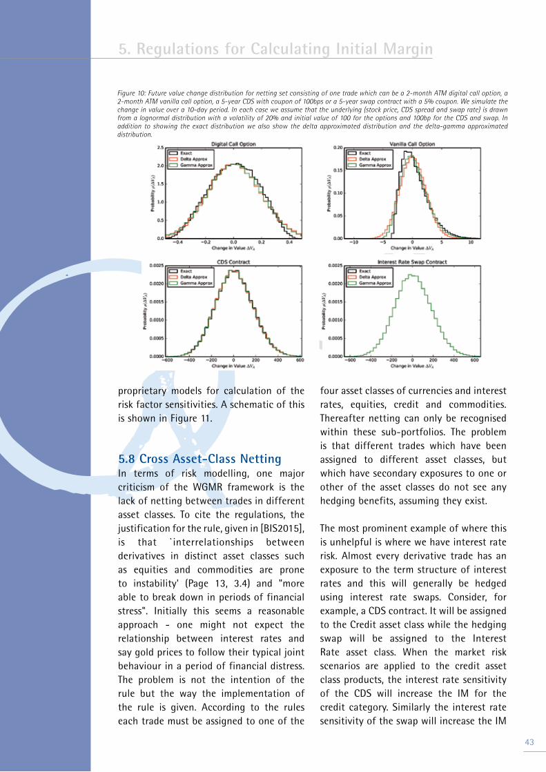
proprietary models for calculation of the risk factor sensitivities. A schematic of this is shown in Figure 11.

5.8 Cross Asset-Class NettingIn terms of risk modelling, one major criticism of the WGMR framework is the lack of netting between trades in different asset classes. To cite the regulations, the justification for the rule, given in [BIS2015], is that ìnterrelationships between derivatives in distinct asset classes such as equities and commodities are prone to instability' (Page 13, 3.4) and "more able to break down in periods of financial stress". Initially this seems a reasonable approach - one might not expect the relationship between interest rates and say gold prices to follow their typical joint behaviour in a period of financial distress. The problem is not the intention of the rule but the way the implementation of the rule is given. According to the rules each trade must be assigned to one of the

four asset classes of currencies and interest rates, equities, credit and commodities. Thereafter netting can only be recognised within these sub-portfolios. The problem is that different trades which have been assigned to different asset classes, but which have secondary exposures to one or other of the asset classes do not see any hedging benefits, assuming they exist.

The most prominent example of where this is unhelpful is where we have interest rate risk. Almost every derivative trade has an exposure to the term structure of interest rates and this will generally be hedged using interest rate swaps. Consider, for example, a CDS contract. It will be assigned to the Credit asset class while the hedging swap will be assigned to the Interest Rate asset class. When the market risk scenarios are applied to the credit asset class products, the interest rate sensitivity of the CDS will increase the IM for the credit category. Similarly the interest rate sensitivity of the swap will increase the IM


43

Figure 10: Future value change distribution for netting set consisting of one trade which can be a 2-month ATM digital call option, a 2-month ATM vanilla call option, a 5-year CDS with coupon of 100bps or a 5-year swap contract with a 5% coupon. We simulate the change in value over a 10-day period. In each case we assume that the underlying (stock price, CDS spread and swap rate) is drawn from a lognormal distribution with a volatility of 20% and initial value of 100 for the options and 100bp for the CDS and swap. In addition to showing the exact distribution we also show the delta approximated distribution and the delta-gamma approximated distribution.

44

for the interest rate asset class products. Even though the interest rate risk has been hedged, the individual IMs will not take this into account and the interest rate risk will be counted twice. This not only ignores the hedging, it actively penalises it. We consider an example.

Example: Consider a e10m 5-year CDS contract with a coupon of 100bp which presents an interest rate exposure that is hedged with a 5-year interest rate swap. Across a range of market par CDS spreads we calculate the swap notional to hedge the interest rate risk. The results are shown in Figure 12. What they show is that the CDS has a very low

interest rate sensitivity such that the amount of swap needed to hedge it is typically 2—8% of the CDS notional. Asthe interest rate risk is counted twice, the IM impact will be twice that of a swap with a notional of e200k-800k.

So from this we conclude that while the IM impact of no cross-asset netting is not significant, it is also far from negligible. Furthermore, a CDS may be considered to be a fairly benign example as its interest rate sensitivity is especially low. It is possible that the impact of no cross-assetnetting would be more significant for other more exotic products. Customised hybrid products that combine two or more


Figure 12: Calculation of the notional size of 5-year interest rate swap needed to hedge a 5-year CDS for a CDS par spread ranging from 1bp to 500bp as a percentage of the CDS notional. The swap is an on-market swap with a coupon of 4.0%.

Figure 11: Initial margin framework design. The scenarios are generated by a public domain scenario generation engine. Each party then combines this with the matrix of first- and second-order sensitivities extracted from their risk-management systems to calculate the distribution of losses from which are calculated the IM amounts.

of interest rate, equity and credit risk will almost certainly be penalised and will likely become more expensive.

This problem can be fixed quite simply. Instead of splitting up trades by their principal risk factor, the guidelines should simply iterate the value of the entire netting set over the individual asset class risk factors, i.e. we calculate the IM for the entire portfolio to interest rate and FX risk, then equity risk, then credit risk and finally commodities risk and sum up the resultingchanges. Such an approach is a minor change to the current framework and would be entirely consistent with the comments of the WGMR on the stability of risk factors.


45

46


Initial margin is intended to protect the non-defaulting counterparty against market price movements following the default of a large counterparty. This is an exceedingly rare event and the only such event in recent times was the Lehman Brothers default of 15 September 2008. It is therefore of interest to briefly examine what impact it had on market prices.

6.1 The Lehman Brothers BankruptcyWe examine the impact of Lehman's bankruptcy on global interest rate swap rates, global equity indices, credit indices and exchange rates over the 10-day period following the Lehman bankruptcy. Table 12 presents the daily change in each of these market factors between 15 and 29 September 2008.33 We note that the Lehman bankruptcy was not the only market-moving event over this period as the $85 billion bailout of AIG occurred on 16 September. We make the following observations:• In the equity market there were some sharp falls, some of which were followed by reversals. The size of equity index price changes did not diminish over the 10-day period, and we saw some large drops at the end of September. Overall the DJ30 fell 9.25% and the FTSE fell 11.04%. Given that equity volatility is typically around 30%, this corresponds to a move of around 1.6 standard deviations over a 10-day period.• The CDS index market widened sharply following the bankruptcy with a 44bp increase in the CDX investment grade index spread on the first trading day and a 25bp increase in the equivalent European index. There were some subsequent narrowings of spreads but overall the CDS spread levels remained around 15bp wider in both the US and Europe at the end of the 10 days.

• Swap rates fell and then rose and fell again across all four currencies shown. The movements in the USD swap rates were higher than those in Europe or Japan. The final change was small given the range of changes over the 10-day period.• The Euro strengthened 1.5% against the dollar following the Lehman bankruptcy while the pound fell by 5.1%.

It is clear that the credit, equity and FX markets reacted significantly to the Lehman bankruptcy. However the 10-day period was not one in which markets moved uniformly in one direction or the other. There were a number of major reversals. The main observation is that daily swings in prices became more extreme than usual. We finally note that the IM add-on, had it been in place, would have been able to cover the 10-day loss in each asset class. In fact it would have covered the worst loss in any of the asset classes over the 10-day period.

6.2 CalibrationFor the purpose of calibrating an IM model, the WGMR has imposed a framework that specifies that model parameters are to be calibrated to a period of 3 to 5 years, and that this must include a period of financial distress. We will now perform some simple calibrations of a range of underlying risk factors that can drive derivative valuations. These will provide simple estimates for a model. By examining different calibration periods it will also be of interest to see theimpact of the inclusion of a period of financial distress. We will also calculate the 99% VaR of a number of individual asset classes in order to see whether the add-ons in Table 9 are consistent with a 99% VaR assumption. Another question of interest is whether the distribution of the market factor can be reasonably approximated

6. Calibration of Asset Classes

4733 - Strictly speaking this is a period of 11 business days. We have added one additional date to account for any delay between the previous VM posting and the bankruptcy announcement.

48

by a Gaussian and we examine this by computing the skew and kurtosis of the distributions.

The regulations for the IM calculation designate four asset classes that a derivative trade must be assigned to. These are (i) currencies and interest rates, (ii) equities, (iii) credit and (iv) commodities. We will consider a model calibration to each of these asset classes. Where the data has been available, we have calibrated to three five-year periods which are 2000-2005, 2005-2010 and 2010-2015. For some assets we only examined 2005-2010 and 2010-2015. Clearly 2005-2010 is the one containing the GFC and so is the only one which would satisfy the regulatory requirements. By examining 2000-2005 and 2010-2015 we can compare the results

to a period which does not include a global financial crisis.

For these periods we calculated the 99th percentile of the resulting distribution. This is the amount of IM that needs to be posted to us by the other counterparty. We also calculate the 1st percentile as the absolute value of this is the amount of IM we must post to the other counterparty. With regard to complex derivatives we have assumed that these can be consideredas delta-weighted amounts of the underlying. For this reason we have only focused on the risk factors of the underlying. This means that we have not include risk factors such as implied volatilities, skews or correlations. This work is beyond the scope of this paper.


Table 12: Daily changes in market prices and spreads over the period prior to and following the bankruptcy of Lehman Brothers on 15 September 2008. The last posting of VM is assumed to be on12 September. This shows changes in some of the major equity indices, the main North American and European investment grade CDS indices (Series 9), 5 year Libor swap rates across four currencies, and two of the main FX rates versus USD. We show the net change in the price or spread or swap rate and then the percentage value change. The bottom row shows the IM add-on for that asset type.

Date Equities CDS Indices 5Y Swap Rates FX (vs $)

DJ30 FTSE iTraxx CDX USD EUR GBP JPY EUR GBP

(% change) (bp change) (bp change) (% change)

9-Sep-08 -2.43 -0.56 2 -3 -5 -5 -3 -2 0.1 -0.3

10-Sep-08 0.34 -0.91 1 6 3 6 0 0 -1.0 0.8

11-Sep-08 1.46 -0.89 1 2 0 4 -6 -1 0 -1.4

12-Sep-08 -0.10 1.85 0 0 7 5 4 2 1.6 0.8

Bankruptcy of Lehman Announced

15-Sep-08 -4.42 -3.92 25 44 -41 -3 -7 -8 0.1 -1.0

16-Sep-08 1.30 -3.43 7 2 11 13 5 -4 -0.8 0.8

17-Sep-08 -4.06 -2.25 9 9 -2 -4 11 2 1.4 -0.5

18-Sep-08 3.86 -0.66 -10 -12 17 21 4 9 0.2 0.4

19-Sep-08 3.35 8.84 -26 -24 33 2 11 5 0.8 -1.1

22-Sep-08 -3.27 -1.41 -3 -7 6 -5 7 -4 2.1 -0.8

23-Sep-08 -1.47 -1.91 7 -10 1 -2 -4 -2 -0.9 -1.8

24-Sep-08 -0.27 -0.79 5 9 7 -2 -5 2 -0.2 -0.6

25-Sep-08 1.82 1.99 -7 4 -2 -3 0 -1 -0.1 -0.5

26-Sep-08 1.10 -2.09 8 -1 -1 -3 -11 4 0.0 0.1

29-Sep-08 -6.98 -5.30 3 0 -33 -15 -12 -2 -1.3 -0.1

Net Change -9 -11 16 14 -4 -2 0 1 1 -5

∆V/V (%) -9 -11 -1 -1 0 0 0 0 1 -5

IM (%) 15 15 5 5 2 2 2 2 6 6

6.3 Currencies and Interest RatesBoth currencies and interest rates are included in the same asset class for the purpose of IM calculation. We consider the calibration to currencies first.

CurrenciesThe currencies component of this asset class needs to cover all of the currencies found in OTC derivative trades. For simplicity we limit ourselves to the major currency pair rates between USD, GBP, EUR and JPY, of which there are six. We calculate the properties of the distribution of percentage changes in the FX rates. The results are shown in Table 13.

We note that the distribution metrics are fairly similar in 2000-2005 and 2010-

2015. In these two periods the skewness is close to zero, as is the kurtosis. This implies that the distributions of returns are symmetric with thinner tails than a Gaussian. In 2005-2010 the distributions are more skewed and, apart from USDJPY, the kurtosis is close to 3 implying that the tails are more Gaussian-like. This is not surprising as this period contained the GFC and so was one in which exchange rates were most volatile. Indeed we see the average volatility over this period being higher than the 2000-2005 and 2010-2015 periods.

The standard add-on for FX derivatives, shown in Table 9, was set at 6%. We see that this is close to the average 99% VaR measure over the period 2005-2010, apart


49

Table 13: The 1st and 99th percentile tail risk measures for the percentage changes in the FX currency pairs listed plus the annualised volatility, skew and kurtosis. We consider three non-overlapping five-year periods with the 2005-2010 being the one that includes the GFC.

2000-2005

1% 99% Skew Kurt Vol (%)

EURUSD -4.43 5.00 -0.04 -0.29 10.33

EURGBP - 3.11 3.71 0.16 -0.14 7.46

EURJPY -5.12 5.81 0.00 0.60 11.04

USDGBP -3.91 3.80 0.15 0.09 8.30

USDJPY -4.17 4.05 -0.01 -0.30 9.25

GBPJPY -4.76 5.15 0.02 0.04 10.37

2005-2010


EURUSD -5.63 5.85 0.29 4.00 10.47

EURGBP -4.16 6.13 0.71 5.19 8.85

EURJPY -7.80 5.34 -1.24 5.21 12.19

USDGBP -4.95 7.15 0.77 2.83 10.99

USDJPY -4.59 4.29 -0.17 0.51 10.15

GBPJPY -9.95 6.27 -0.99 3.87 14.15

2010-2015


EURUSD -4.45 4.43 0.03 0.45 9.12

EURGBP -2.98 3.45 0.29 0.50 6.66

EURJPY -5.17 6.41 0.10 0.57 11.99

USDGBP -3.16 3.82 0.32 0.28 7.54

USDJPY -3.62 5.57 0.48 0.84 9.32

GBPJPY -5.74 5.64 -0.05 0.46 10.89

50

from the case of GBPJPY. It is therefore a parameter choice that agrees well with the initial margin modelling criteria.

Interest RatesAs it is the largest OTC market, it is important for any initial margin model to capture the change in the value of interest rate swaps. The sensitivity at time t of the value of a swap contract, with maturity time T and face value F, to changes in the time T swap rate S(t, T) is given by its DV01 or Dollar Value of 1 basis point. To a first approximation the change in the value of unit notional of a swap contract is

As swaps can have a range of maturities out to over 30 years, a calibration must consider a range of maturity points T. We have chosen the 1, 3, 5, 7, 10, 20 and 30 year points. Swaps in the netting set with maturities that do not fall on these exact tenor points can be modelled as a linear combination of swaps at the two tenor points that bracket their maturity. This canbe done using some combination of a duration, cash flow or variance-preserving mapping.

Using these swap rates and a valuation model to calculate the swap annuity, we have calculated the 1st and 99th percentile changes in the value of a constant tenor swap in all of the main currencies over the periods 2005-2010 and 2010-2015. The results are shown in Table 14. Regarding the VaR percentiles, there are significant variations from currency to currency. For example at the 5Y tenor the 1st and 99th percentiles for JPY are -0.86% and 0.92% respectively. This is materially lower than for EUR and USD which are around -2% to +2%. This can be explained by the very low level of JPY interest rates over the period. We note that the initial margin

add-on for interest rate products shown in Table 9 with 2-5 years to maturity is 2%. This is consistent with what we have found empirically. At longer maturities the 10% initial margin add-on is consistent with what we find for EUR and USD 30Y swaps which show 1st and 99th percentile changes of around 10%.

We also calculated the statistics of changes in the swap rates. These are shown in Table 15. Once again we see that EUR and GBP swap rate changes are about 40bp at the 1st and 99th percentile. For the US they are higher at around 55bp but much lower for JPY which is at around 20bp.Although we find that the percentage volatility in position values was higher during 2010-2015 than over 2005-2010 this is simply because of the much lower level of interest rates over that period. A basis point volatility measure given in Table 15 shows that the basis point volatility of swap rates was higher over 2005-2010 than over 2010-2015.

A typical swap netting set will contain swaps of various maturities. As a result the percentiles of the loss distribution will depend on the correlation between different maturity swap rates. We have estimated the correlation between swap rates over the period 2005-2010 and these are shown in Table 16. As expected, we observe that the swap rate correlation is highest for swap tenors that are close to each other.

6.4 EquitiesIn the case of equities we have focussed on the distribution of returns of the stocks themselves. To perform a calibration, we examined the constituents of each of the major equity stock indices including the French CAC40, the UK FTSE 100, the Italian


MIB, the German Dax 30 and the US Dow Jones index. For each stock in each index we calculated the distribution of 10-day

returns for each stock in each of these indices over the periods 2000-2005, 2005-2010 and 2010-2015.


51

Table 14: VaR measures for 10-day changes in swap values in EUR, GBP, USD and JPY over the period 2005-2010 and 2010-2015 by different swap terms, based on a swap nominal of 100.

EUR Swap Value Changes (%)

Swap 2005-2010 2010-2015

Term 1% 99% 1% 99%

1Y -0.45 0.25 -0.15 0.14

3Y -1.17 1.02 -0.84 0.69

5Y -1.79 1.57 -1.31 1.13

7Y -2.23 1.75 -1.73 1.60

10Y -2.91 2.17 -2.51 2.26

20Y -5.57 3.95 -5.23 4.10

30Y -9.83 5.89 -6.53 5.57

GBP Swap Value Changes (%)

Swap 2005-2010 2010-2015

Term 1% 99% 1% 99%

1Y -0.81 0.32 -0.14 0.13

3Y -1.57 1.38 -0.79 0.77

5Y -2.11 1.87 -1.53 1.49

7Y -2.51 2.08 -1.99 1.96

10Y -3.24 2.25 -2.51 2.36

20Y -4.46 3.71 -3.67 3.34

30Y -6.26 4.43 -4.36 3.79

USD Swap Value Changes (%)

Swap 2005-2010 2010-2015

Term 1% 99% 1% 99%

1Y -0.59 0.43 -0.13 0.14

3Y -1.56 1.38 -0.68 0.79

5Y -2.47 2.21 -1.48 1.63

7Y -3.31 2.99 -2.12 2.33

10Y -4.48 4.12 -2.98 3.06

20Y -7.67 6.64 -5.55 4.46

30Y -10.45 8.43 -7.55 5.50

JPY Swap Value Changes (%)

Swap 2005-2010 2010-2015

Term 1% 99% 1% 99%

1Y -0.11 0.11 -0.03 0.03

3Y -0.49 0.51 -0.21 0.20

5Y -0.86 0.92 -0.50 0.58

7Y -1.16 1.28 -0.76 1.00

10Y -1.52 1.59 -1.24 1.73

20Y -2.73 2.91 -2.50 2.85

30Y -3.68 4.02 -3.27 3.89

52

To summarise our results for each index, we then calculated the average value of the 1st percentile and 99th percentile

measure across all of the constituents of each index. The results are shown in Table 17.


Table 15: VaR measures for 10-day changes in swap rates in EUR, GBP, USD and JPY over the periods 2005-2010 and 2010-2015 by different swap terms. Units are in basis points.

EUR Swap Rates Changes (bp)

Swap 2005-2010 2010-2015

Term 1% 99% 1% 99%

1Y -46.84 26.24 -15.66 -14.80

3Y -42.20 36.80 -30.24 24.79

5Y -40.23 35.37 -29.44 25.39

7Y -37.11 29.10 -28.84 26.73

10Y -35.91 26.73 -30.99 27.84

20Y -40.94 29.03 -38.47 30.17

30Y -56.80 34.02 -37.77 32.20

GBP Swap Rates Changes (bp)

Swap 2005-2010 2010-2015

Term 1% 99% 1% 99%

1Y -84.28 33.48 -14.76 14.02

3Y -56.56 49.67 -28.46 27.87

5Y -47.44 42.08 -34.34 33.49

7Y -41.85 34.60 -33.22 32.59

10Y -39.36 27.70 -30.98 29.06

20Y -32.80 27.28 -26.99 24.58

30Y -36.16 25.60 -25.18 21.91

USD Swap Rates Changes (bp)

Swap 2005-2010 2010-2015

Term 1% 99% 1% 99%

1Y -61.42 44.62 -13.93 14.48

3Y -56.19 49.70 -24.62 28.30

5Y -55.61 49.56 -33.26 36.61

7Y -55.23 49.76 -35.33 38.77

10Y -55.24 50.85 -36.80 37.74

20Y -56.40 48.83 -40.83 32.77

30Y -60.41 48.71 -43.66 31.81

JPY Swap Rates Changes (bp)

Swap 2005-2010 2010-2015

Term 1% 99% 1% 99%

1Y -11.33 11.02 -3.20 2.70

3Y -17.77 18.45 -7.42 7.08

5Y -19.27 20.74 -11.32 13.06

7Y -19.26 21.32 -12.75 16.71

10Y -18.69 19.60 -15.27 21.32

20Y -20.05 21.39 -18.42 20.93

30Y -21.27 23.25 -18.90 22.46

The distributions show that based on a 1st and 99th percentile IM, a change in value of about 15-20% would be expected for equities. This is consistent with the equity add-on used in the standardised approach in Table 9 which is 15%. The stock price change distributions appear to be reasonably symmetric with a slight

positive skew. The average kurtosis is also close to 3, implying that the distributions are Gaussian-like.


53

Table 16: Correlation measures for 10-day changes in swap rates in USD, EUR, GBP and JPY over the period 2005-2010 by different swap terms.

USD Swap Rate Correlations

1Y 3Y 5Y 7Y 10Y 20Y 30Y

1Y 1.000 0.857 0.754 0.674 0.594 0.487 0.453

3Y 0.857 1.000 0.964 0.918 0.857 0.771 0.736

5Y 0.754 0.964 1.000 0.986 0.952 0.883 0.852

7Y 0.674 0.918 0.986 1.000 0.987 0.932 0.903

10Y 0.594 0.857 0.952 0.987 1.000 0.967 0.943

20Y 0.487 0.771 0.883 0.932 0.967 1.000 0.992

30Y 0.453 0.736 0.852 0.903 0.943 0.992 1.000

EUR Swap Rate Correlations

1Y 3Y 5Y 7Y 10Y 20Y 30Y

1Y 1.000 0.858 0.769 0.682 0.572 0.400 0.328

3Y 0.858 1.000 0.964 0.905 0.811 0.636 0.536

5Y 0.769 0.964 1.000 0.978 0.916 0.757 0.651

7Y 0.682 0.905 0.978 1.000 0.974 0.848 0.745

10Y 0.572 0.811 0.916 0.974 1.000 0.922 0.829

20Y 0.400 0.636 0.757 0.848 0.922 1.000 0.968

30Y 0.328 0.536 0.651 0.745 0.829 0.968 1.000

GBP Swap Rate Correlations

1Y 3Y 5Y 7Y 10Y 20Y 30Y

1Y 1.000 0.862 0.785 0.719 0.626 0.468 0.374

3Y 0.862 1.000 0.971 0.920 0.827 0.673 0.566

5Y 0.785 0.971 1.000 0.981 0.922 0.794 0.690

7Y 0.719 0.920 0.981 1.000 0.976 0.875 0.777

10Y 0.626 0.827 0.922 0.976 1.000 0.930 0.847

20Y 0.468 0.673 0.794 0.875 0.930 1.000 0.938

30Y 0.374 0.566 0.690 0.777 0.847 0.938 1.000

JPY Swap Rate Correlations

1Y 3Y 5Y 7Y 10Y 20Y 30Y

1Y 1.000 0.790 0.654 0.555 0.455 0.269 0.203

3Y 0.790 1.000 0.949 0.881 0.788 0.558 0.452

5Y 0.654 0.949 1.000 0.968 0.911 0.693 0.593

7Y 0.555 0.881 0.968 1.000 0.969 0.798 0.707

10Y 0.455 0.788 0.911 0.969 1.000 0.894 0.828

20Y 0.269 0.558 0.693 0.798 0.894 1.000 0.952

30Y 0.203 0.452 0.593 0.707 0.828 0.952 1.000

54

6.5 CreditA significant component of the CDS market, most notably the single-name CDS market, continues to trade in the OTC market. The main CDS indices such as CDX IG and iTraxx Main are now centrally cleared. If we consider the full range of risk factors encountered in non-cleared credit derivatives, these would include spread curves, spread volatility and recover rates. Portfolio products such as bespoke synthetic tranches have an exposure to base correlation. We consider here just the spread risk component. The sensitivity of a $1 nominal long protection CDS position with maturity time T is given by its Credit01 so that we can write

where S(t,T) is the par CDS spread to time

T. We have analysed the distribution of values for a 5-year constant maturity position in the on-the-run (OTR) CDX and iTraxx indices. OTR means that we roll into the new version of the index which is issued semi-annually (typically 20th March or 20th September). The spreads therefore include the effect of composition changes in the index at each roll date.

The results, shown in Table 18 show that the distribution of changes in the value of the CDS is reasonably symmetric. They are around 1-2%. This is much lower than the 5% add-on for 5-year credit in Table 9. However, here we are looking at a CDS index whose price distribution and volatility benefit from diversication. An analysis of single name CDS spreads would almost certainly result in a higher value for the 1st and 99th percentiles.


Table 17: Percentile measures of the 10-day change in stock value averaged over the constituents of the major equity indices shown. This is done for three non-overlapping 5-year periods from 2000 to 2015. We also show the average skew and kurtosis and the annualised volatility.

Index Period 1% 99% Skew Kurt Vol (%)

CAC 2000-2005 20.84 15.63 0.64 2.46 34.61

CAC 2005-2010 21.48 14.76 0.87 3.17 33.38

CAC 2010-2015 15.85 12.46 0.55 1.71 28.30

FTSE 2000-2005 19.31 16.19 0.51 2.30 33.24

FTSE 2005-2010 20.63 16.02 0.69 3.04 33.61

FTSE 2010-2015 13.66 11.20 0.55 2.01 24.91

MIB 2000-2005 18.63 14.80 0.81 4.54 30.98

MIB 2005-2010 21.59 14.96 0.87 3.87 33.04

MIB 2010-2015 18.86 14.47 0.52 1.60 33.94

DAX 2000-2005 22.39 16.59 0.57 2.04 37.23

DAX 2005-2010 21.92 15.62 0.86 3.47 33.93

DAX 2010-2015 15.10 11.44 0.73 2.54 26.70

DJYAHOO 2000-2005 18.98 14.89 0.58 2.19 32.72

DJYAHOO 2005-2010 18.50 13.52 0.83 4.10 28.75

DJYAHOO 2010-2015 10.90 9.13 0.59 1.74 19.98

Table 18: VaR measures for 10-day changes in 5-Year Maturity CDX NA IG OTR and ITraxx Europe OTR index positions in EUR over the period 2010-2015 by different swap terms.

Period 2005-2010 2010-2015

Percentile 1% 99% 1% 9 9%

CDX NA IG -2.01 1.96 -0.69 0.77

ITraxx Europe -1.35 1.67 -1.27 1.26

6.6 CommoditiesWe examined the percentage change in the value of Gold, Silver, Crude Oil, Natural Gas and Wheat futures contracts over the period 2005-2010. From this we calculated the 1st and 99th percentiles of the resulting distributions and these are shown in Table 19.

We see that the distributions are reasonably symmetric, the only one showing any significant skew being natural gas. What is interesting is to compare these percentiles to the standardised IM weight

for commodities which is 15%. We see that this is conservative for gold but on the low side for natural gas. Indeed there seems to be quite a variation in the statistics of thedifferent commodity time series, implying that add-on parameters should be more specific. We also calculated the correlation between the percentage returns of commodities and these are shown in Figure 20. While the correlations are reasonably high, the only two commodities whose price changes are most closely connected are Gold and Silver.


55

Table 19: VaR measures over three non-overlapping periods from 2000-2015 showing the Value at Risk for commodities and different tail probabilities. The annualised volatility of the commodity prices are also shown.

2000-2005

Ticker 1% 99% Skew Kurt Vol (%)

GOLD -5.93 7.41 0.20 0.25 14.03

CRUDE -17.91 16.10 -0.32 0.17 37.35

NATGAS -24.20 36.27 0.69 1.82 61.32

SILVER -13.44 10.86 -0.69 3.63 22.60

WHEAT -9.70 16.09 0.68 0.90 26.71

2005-2010


GOLD -11.39 12.02 -0.29 1.98 22.46

CRUDE -22.43 20.47 -0.17 1.35 40.68

NATGAS -23.09 34.11 0.49 1.28 57.22

SILVER -18.82 17.76 -0.33 0.90 36.27

WHEAT -17.06 19.49 0.26 0.46 37.99

2010-2015


GOLD -9.64 7.64 -0.39 1.00 17.06

CRUDE -15.91 12.44 -0.13 1.49 27.38

NATGAS -16.30 22.18 0.41 0.56 40.11

SILVER -19.73 15.79 -0.28 1.77 33.24

WHEAT -12.72 19.78 0.79 1.46 33.07

Table 20: Correlation matrix for 10-day changes in commodity returns in period 2005-2010.

Gold Crude NatGas Silver Wheat

Gold 1.000 0.300 0.121 0.823 0.229

Crude 0.300 1.000 0.267 0.364 0.231

NatGas 0.121 0.267 1.000 0.218 0.071

Silver 0.823 0.364 0.218 1.000 0.258

Wheat 0.229 0.231 0.071 0.258 1.000

56

The primary market initiative with respect to creating a common standard IM model has been led by ISDA. In December 2013 they published a report, see [ISDA(2014a)], setting out the main requirements of a standard initial margin model (SIMM). This was subsequently updated in March 2014. Since then work has progressed on the model to the extent that a full model description was posted at a special section of ISDA's website34 in October 2015.

7.1 The Model RequirementsIn their first document, ISDA listed the following key requirements for a standard initial margin model (SIMM):1. Easy to replicate: The model should make calculations easy to replicate so that disputes may be avoided.2. Transparent: The model should be fully disclosed to that calculations can be verified as part of any model testing or dispute resolution process.3. Quick: Ideally the calculation should be almost immediate so it can be done intra-day.4. Extensible: The model framework should allow new products and risk factors to be added.5. Predictable: Need to be able to anticipate how IM changes as new trades are added.6. Low cost: Implementation and maintenance and use should not be unduly expensive.7. Governance: The model should be acceptable by dealers and other users and most importantly that it be approved across different regulatory jurisdictions.8. Margin appropriateness: The model recognises risk diversification and hedging.

Of these, perhaps the most important feature of the ISDA framework is its transparency and ease of replication, as the avoidance of disputes will be essential

if the new IM framework is to be workable. In their initial modelling proposal, it seemed as though they were planning a model which would use either historical or Monte-Carlo simulation methods. However in October 2015, ISDA released a new version of their model, with the latest update (version 3.11) in March 2016. Instead of simulation, this one was based on a set of model-calibrated risk weights (tail scenarios) and correlation parameters as we now describe.

This new SIMM methodology borrows significantly from that proposed in the Basel report, the Fundamental Review of the Trading Book35, known as the FRTB. This was issued in October 2013 and it set out a framework for modelling market risk. The SIMM methodology adopts essentially the same risk factors and models them in a similar way. However, despite the similaritybetween the two approaches, they are not the same model. Furthermore, we note that IM is based on a 99% VaR measure while the FRTB proposes the use of a 97.5% expected shortfall. To be more specific, the SIMM approach is most similar to the extended aggregation approach described on page 42 of the FRTB document. This extends the basic FRTB model to include not just linear risk to the principal risk (interest rate, stock price, etc,..), it also incorporates vega and curvature sensitivities. The model is still a work in progress and so our description ofthe model may become out-of-date.

7.2 The Model FrameworkThe ISDA SIMM model is based on the four asset classes chosen by the WGMR, being (i) interest rates and FX, (ii) equities, (iii) credit and (iv) commodities. However the first category is then split into an FX asset class and a general interest rate risk (GIRR) category.

7. The ISDA Standard Initial Margin Model (SIMM)

34 - See http://www2:isda:org/functional-areas/wgmr-implementation/35 - See http://www:bis:org/publ/bcbs265:pdf.

The credit category is split into what is called `Qualifying' and `non-Qualifying' credit. The former consists of investment grade and high-yield credit issued by sovereigns and a wide-range of corporates, while the latter consists of mortgage backed securities. For each of these now six asset classes, the IM amount is given by

The Delta IM is the amount of initial margin needed to protect against changes in the main underlying risk factors for that asset class. For interest rate risk this is the level of a particular swap rate. For equities it is a stock price. For currency derivatives it is an FX rate. The Vega IM is the amount of initial margin needed to protect against a change in volatility and only applies to options or instruments which embed a prepayment option or have some volatility sensitivity. This is also true of the Curvature IM.

One key observation is that the ISDA SIMM model has assumed that model users will be required to split the netting set by product class. This, as we discussed earlier in section 5.8, will prevent the framework from allowing cross-asset class hedging to be taken into account. This is the approach which has been adopted by regulators.

We detail the calculation of the DeltaIM below. We just note that for each asset class, the values of these sensitivities is determined by summing across all of the trades in the netting set. For example the value of DeltaIMGIRR is based on the interest rate risk of all of the trades in the netting set. We can then calculate the IM for each of the four WGMR asset classes.

For the interest rate and FX asset class, this is given by

where the correlation parameter ρ = 0.27. From this, the overall SIMM initial margin can be calculated as follows:

We do not intend to set out the entire SIMM methodology. This can be found in the documents at ISDA's WGMR website. We simply wish to set out the treatment for the calculation of interest rate risk margin IMGIRR in order to give some information about the nature of the implementation and an understanding of the modelling assumptions. Our objective here is to calculate

The methodology for calculating the interest rate sensitivity takes into account the tenor (maturity) of the exposure and the type of interest rate curve. The different tenors captured by the SIMM are 3M, 6M, 1Y, 2Y, 3Y, 5Y, 10Y, 15Y, 20Y and 30Y, making 10 vertices. These are the same as the maturity points used by the FRTB market risk framework. The different curves depend on the currency and then are divided into OIS, Libor1M, Libor3M, Libor6M, Libor12M and Prime (USD only). There is also an inflation factor. The risk factors for interest rates can therefore be labelled with (k, i) where k indexes the tenor and i indexes the curve type. To calculate the overall sensitivity of the netting set, we need the sensitivity to each


57

58

risk factor which is denoted by sk,i. We then have the weighted sensitivity for each tenor and curve type. This is given by

WSk,i = RWksk,i CRb

where CRb is the concentration risk factor for currency b given by

The term inside the square root is the magnitude of the net interest rate sensitivity (summed over tenors and curves) of the netting set divided by the `concentration threshold' Tb, which is currency specific. The concentration thresholds per currency Tb have not yet been determined by ISDA36.

The other term in the weighted sensitivity is the risk-weight RWk. This is specific to the tenor. These are given in Table 21. With this, we can now calculate each value of WSk,i. The next step is to aggregate across curves and tenors within a currency b. The

formula is

We can compare these risk-weights with those estimated earlier and shown in Table 15. For regular currencies we see that the risk-weight is 47, corresponding to 47 basis points. This compares reasonably well to the values of 40bp (35bp), 55bp (50bp) and 47bp (42bp) we found for our 1st (99th) percentile, 2005-2010 calibrations to EUR, USD and GBP swap rates respectively.

The tenor correlation matrix ρk,l is given in Table 22. The sub-curve correlation φi,j is equal to 98.2% for any two curves in the same currency. The values in the correlation matrix are similar to the one we computed earlier shown in Table 16. For example the 1Y-5Y correlation is 75.7% which compares to the 75.4% we found for USD, and the 30Y-5Y correlation is 81.2% which compares to the 85.2% we found for USD.


36 - This is based on Version 3.11 of the ISDA SIMM model methodology.

Table 21: Risk-weights Rk for different currencies. The Regular Currencies include all major currencies (USD, EUR, GBP, CHF, AUD, NZD, CAD, SEK, NOK, DKK, HKD, KRW, SGD, TWD) excluding Japan which is the only one in the Low Volatility category. All other currencies fall into the High Volatility category. These represent the 99th percentiles of the 10-day swap rate changes by tenor and currency.

Tenor 3m 6m 1yr 2yr 3yr 5yr 10yr 15yr 20yr 30yr

Regular Currencies 77 64 58 49 47 47 45 45 48 56

Low Volatility Currencies 10 10 13 16 18 20 25 22 22 23

High Volatility Currencies 89 94 104 99 96 99 87 97 97 98

Table 22: The tenor correlation matrix ρk,l that is used within the ISDA SIMM model for interest rate risk.

Correlation (%)

ρk,l 3m 6m 1yr 2yr 3yr 5yr 10yr 15yr 20yr 30yr

3m 78.2 61.8 49.8 43.8 36.1 27.0 19.6 17.4 12.9

6m 78.2 84.0 73.9 66.7 56.9 44.4 37.5 34.9 29.6

1yr 61.8 84.0 91.7 85.9 75.7 62.6 55.5 52.6 47.1

2yr 49.8 73.9 91.7 97.6 89.5 74.9 69.0 66.0 60.2

3yr 43.8 66.7 85.9 97.6 95.8 83.1 77.9 74.6 69.0

5yr 36.1 56.9 75.7 89.5 95.8 92.5 89.3 85.9 81.2

10yr 27.0 44.4 62.6 74.9 83.1 92.5 98.0 96.1 93.1

15yr 19.6 37.5 55.5 69.0 77.9 89.3 98.0 98.9 97.0

20yr 17.4 34.9 52.6 66.0 74.6 85.9 96.1 98.9 98.8

30yr 12.9 29.6 47.1 60.2 69.0 81.2 93.1 97.0 98.8

The DeltaIMGIRR is then given by aggregating over currencies. We have

where γbc = 0.27 and

This complex looking formula simply caps and floors the summed value of weighted sensitivities to ensure that Sb is in [—Kb,Kb].

In the case of interest rates, the value of the sensitivity s is the change in the value of the trade for a 1bp increase in the risk-factor37. This procedure is then repeated for the vega risk. This involves a sum over trades and a calculation of for each. Curvature risk does not seem to apply to products that have no optionality.

For products that do have a curvature risk,it captures the cross term between the vega and gamma of the option.

Finally we note that, although it is permitted by the WGMR, it is not clear that the SIMM model is intended to model collateral risk (other than FX risk) in order to determine collateral haircuts. There is no reference to such risks in the latest SIMM technical document.

7.3 An Example Calculation of IMLet us consider a simple example that we can compare to the standard approach and to the Alternative NIM approach discussed earlier.


5937 - One-sided or central difference methods can be used.

Example: Consider a netting set consisting of trade 1 which is $15m of a 1Y receiver swap with total DV01 of -$1,200 and trade 2 which is a $5m of 5Y payer swap with total DV01 $2,300. Both are in the same currency (USD) and so both exposed to the same interest rate curve. These have no vega. We ignore curvature risk. The value of the weighted sensitivities are

We have yet to calculate CRb. As Tb has not yet been determined, we set CRb = 1. Substituting for the values of the risk-weights we get (for simplicity we quote sensitivities in $000's)

We then aggregate these numbers to give

The correlation parameter is 75.7% and as we are using the same sub-curve in the same currency we set φ = 1.0. As we have only one country (EUR) in the netting set,

This corresponds to $71,690. We can compare this to the standard approach. We first calculate the Gross Initial Margin as follows

60

In an attempt to create a common standard for the various IM models currently in construction, ISDA began tendering in June 2015 for a third party to build and operate a crowdsourced utility to enable market participants to implement the ISDA SIMM consistently. It appears that the scope for this utility is to ensure the consistent treatment of risk-weights and correlation parameters across users of the SIMM model. In September 2015, the ICE Benchmark Administration Ltd. (IBA) was selected for this task. It certainly seems as though the ISDA SIMM may become the market-wide standard model for IM calculation.


Assuming that the values of the two swaps are exactly offsetting so that the NGR is zero, we have

So even in the best case, when the NGR is zero, the IM charge is more than twice that produced by the SIMM. We can also compare this result to the Alternative NIM model suggested earlier.In this case we would have computed

This is less than the amount calculated by the SIMM. It reflects the fact that the Alternative NIM model assumes only parallel movements in the interest rate curve so that the correlation assumption is essentially 100%. We therefore benefit more than we ought to from the offsettingswap positions.

In this report we have provided an overview of the new initial margin regulations that will come into effect for non-cleared OTC derivatives in September of this year. We have then set out in detail the two approaches that the WGMR has provided for calculation of IM and commented on their appropriateness.

With respect to total market liquidity, we note that VM should have no overall impact on market users but that IM does impact market-wide liquidity as the IM collateral cannot be re-used or re-hypothecated except in a fairly narrow set of circumstances.

We have examined the standardised approach to calculating IM and found that it does not account correctly for the overall sensitivity of the value of the netting set to market risk. The Net-to-Gross-Ratio (NGR) metric incorrectly uses trade values as a proxy for trade sensitivities. It also ignores the delta sensitivity of option products. We show that this approach overstates the amount of initial margin required. We conclude that the standard approach can only be acceptable to counterparties with simple non-offsetting positions for whom the model-based approach provides few if any additional benefits.

The second approach for determining IM is based on an approved initial margin model. While the choice of model to be used is left open, the metric to be used for determining the IM charge is explicitly stated to be the 99th percentile of the value change distribution of the netting set. The WGMR also states that the calibration period for a model should be based on a 3 to 5 year window that includes a period of financial distress. We believe that the imposition of a clearly defined metric is helpful, primarily because there is very little data

to enable the calibration of a model to the rare event of counterparty default and its subsequent impact on market prices. The approved initial margin model allows us to take trade diversification into account correctly. Second, it allows the market risk sensitivities of options and other complex derivatives to be treated correctly. Third, it acknowledges that the IM charge is not symmetric and so can be different for both counterparties.

There is no explicit mention of the issue of procyclicality in the IM model framework. As discussed in [Murphy(2014)], the concern is that models that reflect recent changes in volatility, which are generally associated with periods of financial distress, will lead to higher initial margin charges just when financial institutions are least able to fund them. The requirement that calibration data must cover a period of 3 to 5 years (1 to 5 years in the US), be equally weightedthrough time, and contain a period of financial distress, means that the volatility calibration will not be so sensitive to recent events.

The challenge of designing and building an IM model, and having it approved is significant. Repeating this process for every covered entity will take time and be expensive. It is therefore very welcome that ISDA has chosen to specify a single modelling approach that might be adoptedacross the market. We have described this model, noting that it is not final. The modelling framework is fairly simple and involves bringing together stressed risk factors and risk sensitivities computed by counterparties to produce an IM amount. The nature of the model means that given the supplied risk sensitivities, calculation of the IM should be more or less instant. It appears that the model will take into account both linear and curvature effects

8. Discussion

61

62

of the risk factors, which may be required for some products. Also, the model handles option implied volatility sensitivities in a fairly advanced way. Finally, the fact that it borrows much from the BIS FTRB approachshould assist it in obtaining regulatory approval. Assuming that the SIMM model proposed by ISDA obtains regulatory approval, it appears that the market will be able unite around this framework for IM calculations. This will significantly reduce the potential for disputes that would have occurred if the market had fragmented around different IM models.

Initial margin is a form of insurance against a contingent risk that banks face when they trade non-cleared OTC derivatives. It is hoped that its introduction will lead to safer and smoother-functioning OTC derivative markets. However, the defaulter pays requirement means that this will come at a cost, the cost of providing all counterparties tying up significant amounts of collateral that may not be reused or rehypothecated. It remains to be seen whether this cost will fall inside the range that it does reduce market systemic risk while allowing many market players to continue to participate and provide liquidity to non-cleared OTC derivative markets.

8. Discussion

• Artzner, P. F. Delbaen, J.M. Eber and D. Heath. 1999. Coherent Measures of Risk. Mathematical Finance 9(3): 203-228.

• BIS. 2015. Margin requirements for non-centrally cleared derivatives, Bank Committee on Banking Supervision. (March).

• Glasserman, P, P. Heidelberger and P. Shahabuddin. 2001. Efficient Monte Carlo methods for value-at-risk in Mastering Risk: Application. Volume 2, (August).

• Gregory, J. 2015. The xVA Challenge: Counterparty Credit Risk, Funding, Collateral and Capital. Wiley Finance, 3rd Edition.

• ISDA. 2014a. ISDA Standard Initial Margin Model for Non-Cleared Derivatives, International Swaps and Derivatives Association. (March).

• ISDA. 2014b. ISDA Size and Uses of the Non-Cleared Derivatives Market, International Swaps and Derivatives Association (April).

• Murphy, D. 2013. OTC Derivatives: Bilateral Trading and Central Clearing, Palgrave Macmillan.

• Murphy, D., M. Vasios and N. Vause. 2014. An investigation into the pro-cyclicality of risk-based initial margin models. Bank of England, Financial Stability Paper No. 29.

References

63

64

2016 Publications• Amenc, N., F. Goltz, V. Le Sourd, A. Lodh and S. Sivasubramanian. The EDHEC European ETF Survey 2015 (February).

• Martellini, L. Mass Customisation versus Mass Production in Investment Management (January).

2015 Publications• Blanc-Brude, F., M. Hasan and T. Whittaker. Cash Flow Dynamics of Private Infrastructure Project Debt (November).

• Amenc, N., G. Coqueret and L. Martellini. Active Allocation to Smart Factor Indices (July).

• Martellini, L. and V. Milhau. Factor Investing: A Welfare Improving New Investment Paradigm or Yet Another Marketing Fad? (July).

• Goltz, F. and V. Le Sourd. Investor Interest in and Requirements for Smart Beta ETFs (April).

• Amenc, N., F. Goltz, V. Le Sourd and A. Lodh. Alternative Equity Beta Investing: A Survey (March).

• Amenc, N., K. Gautam, F. Goltz, N. Gonzalez and J.P Schade. Accounting for Geographic Exposure in Performance and Risk Reporting for Equity Portfolios (March).

• Amenc, N., F. Ducoulombier, F. Goltz, V. Le Sourd, A. Lodh and E. Shirbini. The EDHEC European Survey 2014 (March).• Deguest, R., L. Martellini, V. Milhau, A. Suri and H. Wang. Introducing a Comprehensive Investment Framework for Goals-Based Wealth Management (March).

• Blanc-Brude, F. and M. Hasan. The Valuation of Privately-Held Infrastructure Equity Investments (January).

2014 Publications• Coqueret, G., R. Deguest, L. Martellini and V. Milhau. Equity Portfolios with Improved Liability-Hedging Benefits (December).

• Blanc-Brude, F. and D. Makovsek. How Much Construction Risk do Sponsors take in Project Finance. (August).

• Loh, L. and S. Stoyanov. The Impact of Risk Controls and Strategy-Specific Risk Diversification on Extreme Risk (August).

• Blanc-Brude, F. and F. Ducoulombier. Superannuation v2.0 (July).

• Loh, L. and S. Stoyanov. Tail Risk of Smart Beta Portfolios: An Extreme Value Theory Approach (July).

• Foulquier, P. M. Arouri and A. Le Maistre. P. A Proposal for an Interest Rate Dampener for Solvency II to Manage Pro-Cyclical Effects and Improve Asset-Liability Management (June).

• Amenc, N., R. Deguest, F. Goltz, A. Lodh, L. Martellini and E.Schirbini. Risk Allocation, Factor Investing and Smart Beta: Reconciling Innovations in Equity Portfolio Construction (June).

• Martellini, L., V. Milhau and A. Tarelli. Towards Conditional Risk Parity — Improving Risk Budgeting Techniques in Changing Economic Environments (April).

• Amenc, N. and F. Ducoulombier. Index Transparency – A Survey of European Investors Perceptions, Needs and Expectations (March).

• Ducoulombier, F., F. Goltz, V. Le Sourd and A. Lodh. The EDHEC European ETF Survey 2013 (March).

EDHEC-Risk Institute Position Papers and Publications (2013-2016)


• Badaoui, S., Deguest, R., L. Martellini and V. Milhau. Dynamic Liability-Driven Investing Strategies: The Emergence of a New Investment Paradigm for Pension Funds? (February).

• Deguest, R. and L. Martellini. Improved Risk Reporting with Factor-Based Diversification Measures (February).

• Loh, L. and S. Stoyanov. Tail Risk of Equity Market Indices: An Extreme Value Theory Approach (February).

2014 Position Papers• Blanc-Brude, F. Benchmarking Long-Term Investment in Infrastructure: Objectives, Roadmap and Recent Progress (June).

2013 Publications• Loh, L. and S. Stoyanov. Tail Risk of Asian Markets: An Extreme Value Theory Approach (August).

• Goltz, F., L. Martellini and S. Stoyanov. Analysing statistical robustness of cross-sectional volatility. (August).

• Loh, L., L. Martellini and S. Stoyanov. The local volatility factor for asian stock markets. (August).

• Martellini, L. and V. Milhau. Analyzing and decomposing the sources of added-value of corporate bonds within institutional investors’ portfolios (August).

• Deguest, R., L. Martellini and A. Meucci. Risk parity and beyond - From asset allocation to risk allocation decisions (June).

• Blanc-Brude, F., Cocquemas and F. Georgieva, A. Investment Solutions for East Asia's Pension Savings - Financing lifecycle deficits today and tomorrow (May)

• Blanc-Brude, F. and O.R.H. Ismail. Who is afraid of construction risk? (March)

• Loh, L., L. Martellini and S. Stoyanov. The relevance of country- and sector-specific model-free volatility indicators (March).

• Calamia, A., L. Deville and F. Riva. Liquidity in european equity ETFs: What really matters? (March).

• Deguest, R., L. Martellini and V. Milhau. The benefits of sovereign, municipal and corporate inflation-linked bonds in long-term investment decisions (February).

• Deguest, R., L. Martellini and V. Milhau. Hedging versus insurance: Long-horizon investing with short-term constraints (February).

• Amenc, N., F. Goltz, N. Gonzalez, N. Shah, E. Shirbini and N. Tessaromatis. The EDHEC european ETF survey 2012 (February).

• Padmanaban, N., M. Mukai, L. Tang and V. Le Sourd. Assessing the quality of asian stock market indices (February).

• Goltz, F., V. Le Sourd, M. Mukai and F. Rachidy. Reactions to “A review of corporate bond indices: Construction principles, return heterogeneity, and fluctuations in risk exposures” (January).

• Joenväärä, J. and R. Kosowski. An analysis of the convergence between mainstream and alternative asset management (January).

• Cocquemas, F. Towar¬ds better consideration of pension liabilities in european union countries (January). 65

• Blanc-Brude, F. Towards efficient benchmarks for infrastructure equity investments (January).


66

Founded in 1906, EDHEC Business School offers management education at undergraduate, graduate, post-graduate and executive levels. Holding the AACSB, AMBA and EQUIS accreditations and regularly ranked among Europe’s leading institutions, EDHEC Business School delivers degree courses to over 6,500 students from the world over and trains 10,000 professionals yearly through executive courses and research events. The School’s ‘Research for Business’ policy focuses on issues that correspond to genuine industry and community expectations.

Part of EDHEC Business School and established in 2001, EDHEC-Risk Institute has become the premier academic centre for industry-relevant financial research. In partnership with large financial institutions, its team of close to 50 permanent professors, engineers, and support staff, and 38 research associates and affiliate professors, implements 6 research programmes and 10 research chairs focusing on asset allocation and risk management and has

developed an ambitious portfolio of research and educational initiatives in the domain of investment solutions for institutional and individual investors. EDHEC-Risk Institute also has highly significant executive education activities for professionals. In partnership with CFA Institute, it has developed advanced seminars based on its research which are available to CFA charterholders and have been taking place since 2008 in New York, Singapore and London.

In 2012, EDHEC-Risk Institute signed two strategic partnership agreements, with the Operations Research and Financial Engineering department of Princeton University to set up a joint research programme in the area of asset-liability management for institutions and individuals, and with Yale School of Management to set up joint certified executive training courses in North America and Europe in the area of risk and investment management.

Copyright © 2016 EDHEC-Risk Institute

For more information, please contact: Carolyn Essid on +33 493 187 824 or by e-mail to: [email protected]

EDHEC-Risk Institute393 promenade des AnglaisBP 3116 - 06202 Nice Cedex 3FranceTel: +33 (0)4 93 18 78 24

EDHEC Risk Institute—Europe 10 Fleet Place, LudgateLondon EC4M 7RBUnited KingdomTel: +44 207 871 6740

EDHEC Risk Institute—Asia1 George Street#07-02Singapore 049145Tel: +65 6438 0030

EDHEC Risk Institute—France 16-18 rue du 4 septembre75002 Paris FranceTel: +33 (0)1 53 32 76 30

www.edhec-risk.com

Institute