Higher-Order Concurrency: Expressiveness andDecidability Results
Jorge A. Perez P.
Technical Report UBLCS-2010-07
March 2010
Department of Computer ScienceUniversity of BolognaMura Anteo Zamboni 740127 Bologna (Italy)

The University of Bologna Department of Computer Science Research Technical Reports
are available in PDF and gzipped PostScript formats via anonymous FTP from the area
ftp.cs.unibo.it:/pub/TR/UBLCS or via WWW at URL http://www.cs.unibo.it/. Plain-
text abstracts organized by year are available in the directory ABSTRACTS.
Recent Titles from the UBLCS Technical Report Series
2008-18 Lebesgue’s Dominated Convergence Theorem in Bishop’s Style, Sacerdoti Coen, C., Zoli, E., Novem-
ber 2008.
2009-01 A Note on Basic Implication, Guidi, F., January 2009.
2009-02 Algorithms for network design and routing problems (Ph.D. Thesis), Bartolini, E., February 2009.
2009-03 Design and Performance Evaluation of Network on-Chip Communication Protocols and Architectures
(Ph.D. Thesis), Concer, N., February 2009.
2009-04 Kernel Methods for Tree Structured Data (Ph.D. Thesis), Da San Martino, G., February 2009.
2009-05 Expressiveness of Concurrent Languages (Ph.D. Thesis), di Giusto, C., February 2009.
2009-06 EXAM-S: an Analysis tool for Multi-Domain Policy Sets (Ph.D. Thesis), Ferrini, R., February 2009.
2009-07 Self-Organizing Mechanisms for Task Allocation in a Knowledge-Based Economy (Ph.D. Thesis), Mar-
cozzi, A., February 2009.
2009-08 3-Dimensional Protein Reconstruction from Contact Maps: Complexity and Experimental Results
(Ph.D. Thesis), Medri, F., February 2009.
2009-09 A core calculus for the analysis and implementation of biologically inspired languages (Ph.D. Thesis),
Versari, C., February 2009.
2009-10 Probabilistic Data Integration, Magnani, M., Montesi, D., March 2009.
2009-11 Equilibrium Selection via Strategy Restriction in Multi-Stage Congestion Games for Real-time Stream-
ing, Rossi, G., Ferretti, S., D’Angelo, G., April 2009.
2009-12 Natural deduction environment for Matita, C. Sacerdoti Coen, E. Tassi, June 2009.
2009-13 Hints in Unification, Asperti, A., Ricciotti, W., Sacerdoti Coen, C., Tassi, E., June 2009.
2009-14 A New Type for Tactics, Asperti, A., Ricciotti, W., Sacerdoti Coen, C., Tassi, E., June 2009.
2009-15 The k-Lattice: Decidability Boundaries for Qualitative Analysis in Biological Languages, Delzanno,
G., Di Giusto, C., Gabbrielli, M., Laneve, C., Zavattaro, G., June 2009.
2009-16 Landau’s ”Grundlagen der Analysis” from Automath to lambda-delta, Guidi, F., September 2009.
2010-01 Fast overlapping of protein contact maps by alignment of eigenvectors, Di Lena, P., Fariselli, P., Mar-
gara, L., Vassura, M., Casadio, R., January 2010.
2010-02 Optimized Training of Support Vector Machines on the Cell Processor, Marzolla, M., February 2010.
2010-03 Modeling Self-Organizing, Faulty Peer-to-Peer Systems as Complex Networks Ferretti, S., February
2010.

iii
2010-04 The qnetworks Toolbox: A Software Package for Queueing Networks Analysis, Marzolla, M., Febru-
ary 2010.
2010-05 QoS Analysis for Web Service Applications: a Survey of Performance-oriented Approaches from an
Architectural Viewpoint, Marzolla, M., Mirandola, R., February 2010.
2010-06 The dark side of the board: advances in Kriegspiel Chess (Ph.D. Thesis), Favini, G.P., March 2010.


Dottorato di Ricerca in InformaticaUniversita di Bologna e PadovaINF/01 INFORMATICACiclo XXII
Higher-Order Concurrency: Expressiveness andDecidability Results
Jorge A. Perez P.March 2010
Coordinatore: Tutore:Prof. Simone Martini Prof. Davide Sangiorgi

vi
Higher-Order Concurrency: Expressiveness and Decidability Results
Higher-order process calculi are formalisms for concurrency in which processes can be passedaround in communications. Higher-order (or process-passing) concurrency is often presentedas an alternative paradigm to the first order (or name-passing) concurrency of the π-calculusfor the description of mobile systems. These calculi are inspired by, and formally close to, theλ-calculus, whose basic computational step β-reduction involves term instantiation.The theory of higher-order process calculi is more complex than that of first-order processcalculi. This shows up in, for instance, the definition of behavioral equivalences. A long-standing approach to overcome this burden is to define encodings of higher-order processesinto a first-order setting, so as to transfer the theory of the first-order paradigm to the higher-order one. While satisfactory in the case of calculi with basic (higher-order) primitives, thisindirect approach falls short in the case of higher-order process calculi featuring constructsfor phenomena such as, e.g., localities and dynamic system reconfiguration, which are frequentin modern distributed systems. Indeed, for higher-order process calculi involving little morethan traditional process communication, encodings into some first-order language are difficultto handle or do not exist. We then observe that foundational studies for higher-order processcalculi must be carried out directly on them and exploit their peculiarities.This dissertation contributes to such foundational studies for higher-order process calculi.We concentrate on two closely interwoven issues in process calculi: expressiveness and decid-ability. Surprisingly, these issues have been little explored in the higher-order setting. Ourresearch is centered around a core calculus for higher-order concurrency in which only theoperators strictly necessary to obtain higher-order communication are retained. We developthe basic theory of this core calculus and rely on it to study the expressive power of issuesuniversally accepted as basic in process calculi, namely synchrony, forwarding, and polyadiccommunication.
Keywords: concurrency theory, process calculi, higher-order communication, expressiveness,decidability.


Acknowledgments
My greatest debt is to Davide Sangiorgi. Having him as supervisor has been truly inspiring.His careful supervision has influenced enormously my way of doing (and approaching) research.His continuous support and patience during these three years were fundamental to me. I amstill amazed by the fact that Davide had always time for me, not only for scientific discussionsbut also for sorting out everyday issues. I am most grateful to him for his honest and directadvice, and for the liberty that he gave me during my studies.I also owe much to Camilo Rueda and Frank D. Valencia. I do not forget that it was Camilowho introduced me to research, thus giving me an opportunity that most people in his positionwould have refused. Even if my PhD studies were not directly related to his research interests,Camilo was always there, interested in my progresses, encouraging me with his support andfriendship. Frank not only introduced me to concurrency theory; he also gave me constantadvise and support during my PhD studies and long before. Frank had a lot to do with mecoming to Bologna, and that I will never forget.There is no way in which I could have completed this dissertation by myself. It has been apleasure to collaborate with extremely talented people, to whom I am deeply grateful: CinziaDi Giusto, Ivan Lanese, Alan Schmitt, Gianluigi Zavattaro. Thank you for your kindness,generosity and, above all, for your patience.Many thanks to Uwe Nestmann and Nobuko Yoshida for having accepted to review thisdissertation. Thanks also to the members of my internal committee (commissione), CosimoLaneve and Claudio Sacerdoti-Coen. I am indebted to Simone Martini, the coordinator of thePhD program, for all his constant availability and kindness.Many people proof-read parts of this dissertation, and provided me with constructive crit-icisms. I am grateful to all of them for their time and availability: Jesus Aranda, AlbertoDelgado, Cinzia Di Giusto, Daniele Gorla, Julian Gutierrez, Hugo A. Lopez, Claudio Mezzina,Margarida Piriquito, Frank D. Valencia. A special thanks goes to Daniele Varacca, who suf-fered an early draft of the whole document and provided me with insightful remarks. Alongthese years I have benefited a lot from discussions with/comments from a lot of people. Iam most grateful for their positive attitude towards my work: Jesus Aranda, Ahmed Bouaj-jani, Gerard Boudol, Santiago Cortes, Rocco De Nicola, Daniele Gorla, Matthew Hennessy,
x
Thomas Hildebrandt, Kohei Honda, Roland Meyer, Fabrizio Montesi, Camilo Rueda, Jean-Bernard Stefani, Frank D. Valencia, Daniele Varacca, Nobuko Yoshida.During 2009 I spent some months visiting Alan Schmitt in the SARDES team at INRIAGrenoble - Rhone-Alpes. The period in Grenoble was very enriching and productive; a sub-stantial part of this dissertation was written there. I am grateful to Alan and to Jean-BernardStefani for the opportunity of working with them and for treating me as another member ofthe team. I would like to thank Diane Courtiol for her patient help with all the administrativeissues during my stay, and to Claudio Mezzina (or the “tiny little Italian with a pony tail”,as he requested to be acknowledged) for being such a friendly office mate. I also thank theINRIA Equipe Associee BACON for partially supporting my visit.I would like to express my appreciation to the University of Bologna - MIUR for supportingmy studies through a full scholarship. Thanks also to the administrative staff in the Departmentof Computer Science, for their help and kindness in everyday issues.I am most proud to be part of a small group of Colombians doing research abroad. Weall share many things: we started in the same research group, have similar backgrounds, andcame to Europe more or less at the same time. With most of them I even shared an office fora long time. Many thanks to: Jesus Aranda, for his inherent kindness; Alejandro Arbelaez, forthe good times while working in Colombia and his hospitality during trips to Paris; AndresAristizabal, for the constant support in spite of our favorite football teams; Alberto Delgado,with whom I started doing research back in 2002 and has always been there ever since;Gustavo Gutierrez, for the old, good times when he was my first boss, and for the sinceresupport during all these years; Julian Gutierrez, for all the discussions on life and research,during our PhDs and even way before; Hugo A. Lopez, for sharing with me the experienceof living in Italy, several trips, and a plenty of discussions on concurrency theory and lifeat large; Carlos Olarte, for all the good times in Paris and hospitality in the great city ofBourg-la-Reine; Luis O. Quesada, for his exceptional kindness and hospitality during a visitto Ireland (despite of the fact that my visit brought historical floodings to the Cork region).Above all, I would like to thank all of them for being my friends.Perhaps the most significant achievement of my PhD studies is all the people I have meetalong the way. A special thanks goes to: Cinzia Di Giusto, for her constant support andfriendship, and for being the most enthusiastic partner in research one could imagine; AntonioVitale, for the several trips and for sharing with me bits of PhD frustration and pizzas of varyingquality; Ivan Lanese, the loyal friend, the reasonable flat mate, and the talented co-author.Thanks also to: Stefano Arteconi, for insightful and enjoyable discussions on Italy, movies, andmusic; Ferdinanda Camporesi, for the many chats and the movies we watched together; MarcoDi Felice, for being the most welcoming and friendly office mate in underground and beingworse than me in calcetto; Ebbe Elsborg (and family) the most loyal reader of my blog for
xi
his kind hospitality during the most splendid vacation in Denmark I could have imagined, andfor plenty of discussions on pretty much every aspect of life; Elena Giachino and Luis Perez,for all the fun we had together at summer schools, and for dinners and parties at Pisa; ZeynepKiziltan, for the chats over lunch that didn’t deal about work; Flavio S. Mendes, for the manytrips we did together around Italy, the constant support and friendship, and the many times Istayed at his place; Margarida Piriquito, for the most unexpected friendship I can remember;Sylvain Pradalier, or the coolest French guy I could have shared an office with; Alan Schmitt(and family), for the several great dinners at his place (in Grenoble, but also in Casalecchio)and the clever games in which I would always lose no matter how hard I would try.Last but not least, I would like to thank my family for their unconditional, constant support.There are no words to thank my parents, my sisters, my brother, and my grandmother. Theirlove gave me strength to overcome the difficult times. I would also like to thank Andres F.Monsalve, who is more like a brother than a friend to me. Thanks also to the rest of my family,the many cousins, uncles, and aunts for their continued support towards me.


Contents
Acknowledgments ix
List of Figures xvii
1 Introduction 11.1 Context and Motivation . . . . . . . . . . . . . . . . . . . . . . . . . . . . . . . . . 11.2 First-Order and Higher-Order Concurrency . . . . . . . . . . . . . . . . . . . . . 41.3 This Dissertation . . . . . . . . . . . . . . . . . . . . . . . . . . . . . . . . . . . . . 91.3.1 Expressiveness and Decidability in Higher-Order Concurrency . . . . . . 91.3.2 Approach . . . . . . . . . . . . . . . . . . . . . . . . . . . . . . . . . . . . . 111.3.3 Contributions and Structure . . . . . . . . . . . . . . . . . . . . . . . . . . 122 Preliminaries 152.1 Technical Background . . . . . . . . . . . . . . . . . . . . . . . . . . . . . . . . . . 152.1.1 Bisimilarity . . . . . . . . . . . . . . . . . . . . . . . . . . . . . . . . . . . . 152.1.2 A Calculus of Communicating Systems . . . . . . . . . . . . . . . . . . . . 172.1.3 More on Behavioral Equivalences . . . . . . . . . . . . . . . . . . . . . . . 192.1.4 A Calculus of Mobile Processes . . . . . . . . . . . . . . . . . . . . . . . . 212.2 Higher-Order Process Calculi . . . . . . . . . . . . . . . . . . . . . . . . . . . . . 252.2.1 The Higher-Order π-calculus . . . . . . . . . . . . . . . . . . . . . . . . . 262.2.2 Sangiorgi’s Representability Result . . . . . . . . . . . . . . . . . . . . . . 272.2.3 Other Higher-Order Languages . . . . . . . . . . . . . . . . . . . . . . . . 292.2.4 Behavioral Theory . . . . . . . . . . . . . . . . . . . . . . . . . . . . . . . . 342.3 Expressiveness of Concurrent Languages . . . . . . . . . . . . . . . . . . . . . . . 372.3.1 Generalities . . . . . . . . . . . . . . . . . . . . . . . . . . . . . . . . . . . 382.3.2 The Notion of Encoding . . . . . . . . . . . . . . . . . . . . . . . . . . . . 402.3.3 Main Approaches to Expressiveness . . . . . . . . . . . . . . . . . . . . . 472.3.4 Expressiveness for Higher-Order Languages . . . . . . . . . . . . . . . . 52
xiv Contents
3 A Core Calculus for Higher-Order Concurrency 55
3.1 The Calculus . . . . . . . . . . . . . . . . . . . . . . . . . . . . . . . . . . . . . . . 553.2 Expressiveness of HOCORE . . . . . . . . . . . . . . . . . . . . . . . . . . . . . . . 57
3.2.1 Guarded Choice . . . . . . . . . . . . . . . . . . . . . . . . . . . . . . . . . 573.2.2 Input-guarded Replication . . . . . . . . . . . . . . . . . . . . . . . . . . . 583.2.3 Minsky machines . . . . . . . . . . . . . . . . . . . . . . . . . . . . . . . . 58
3.3 Concluding Remarks . . . . . . . . . . . . . . . . . . . . . . . . . . . . . . . . . . . 644 Behavioral Theory of HOCORE 65
4.1 Bisimilarity in HOCORE . . . . . . . . . . . . . . . . . . . . . . . . . . . . . . . . . 654.2 Barbed Congruence and Asynchronous Equivalences . . . . . . . . . . . . . . . . 744.3 Axiomatization and Complexity . . . . . . . . . . . . . . . . . . . . . . . . . . . . . 77
4.3.1 Axiomatization . . . . . . . . . . . . . . . . . . . . . . . . . . . . . . . . . . 784.3.2 Complexity of Bisimilarity Checking . . . . . . . . . . . . . . . . . . . . . 81
4.4 Bisimilarity is Undecidable with Four Static Restrictions . . . . . . . . . . . . . 844.5 Other Extensions . . . . . . . . . . . . . . . . . . . . . . . . . . . . . . . . . . . . . 884.6 Concluding Remarks . . . . . . . . . . . . . . . . . . . . . . . . . . . . . . . . . . . 89
5 On the Expressiveness of Forwarding and Suspension 91
5.1 Introduction . . . . . . . . . . . . . . . . . . . . . . . . . . . . . . . . . . . . . . . . 925.2 The Calculus . . . . . . . . . . . . . . . . . . . . . . . . . . . . . . . . . . . . . . . 945.3 Convergence is Undecidable in HO−f . . . . . . . . . . . . . . . . . . . . . . . . . 95
5.3.1 Encoding Minsky Machines into HO−f . . . . . . . . . . . . . . . . . . . . 965.3.2 Correctness of the Encoding . . . . . . . . . . . . . . . . . . . . . . . . . . 98
5.4 Termination is Decidable in HO−f . . . . . . . . . . . . . . . . . . . . . . . . . . . 1055.4.1 Well-Structured Transition Systems . . . . . . . . . . . . . . . . . . . . . 1055.4.2 A Finitely Branching LTS for HO−f . . . . . . . . . . . . . . . . . . . . . . 1075.4.3 Termination is Decidable in HO−f . . . . . . . . . . . . . . . . . . . . . . . 109
5.5 On the Interplay of Fowarding and Passivation . . . . . . . . . . . . . . . . . . . 1185.5.1 A Faithful Encoding of Minsky Machines into HOP−f . . . . . . . . . . . 1185.5.2 Correctness of the Encoding . . . . . . . . . . . . . . . . . . . . . . . . . . 120
5.6 Concluding Remarks . . . . . . . . . . . . . . . . . . . . . . . . . . . . . . . . . . . 123

Contents xv
6 On the Expressiveness of Synchronous/Polyadic Communication 1276.1 Introduction . . . . . . . . . . . . . . . . . . . . . . . . . . . . . . . . . . . . . . . . 1276.2 The Calculi . . . . . . . . . . . . . . . . . . . . . . . . . . . . . . . . . . . . . . . . 1326.2.1 A Higher-Order Process Calculus with Restriction and Polyadic Com-munication . . . . . . . . . . . . . . . . . . . . . . . . . . . . . . . . . . . . 1326.2.2 A Higher-Order Process Calculus with Synchronous Communication . . 1346.3 The Notion of Encoding . . . . . . . . . . . . . . . . . . . . . . . . . . . . . . . . . 1356.4 An Encodability Result for Synchronous Communication . . . . . . . . . . . . . . 1376.5 Separation Results for Polyadic Communication . . . . . . . . . . . . . . . . . . . 1386.5.1 Distinguished Forms . . . . . . . . . . . . . . . . . . . . . . . . . . . . . . 1396.5.2 A Hierarchy of Synchronous Higher-Order Process Calculi . . . . . . . . 1456.6 The Expressive Power of Abstraction Passing . . . . . . . . . . . . . . . . . . . . 1506.7 Concluding Remarks . . . . . . . . . . . . . . . . . . . . . . . . . . . . . . . . . . . 1527 Conclusions and Perspectives 1557.1 Concluding Remarks . . . . . . . . . . . . . . . . . . . . . . . . . . . . . . . . . . . 1557.2 Ongoing and Future Work . . . . . . . . . . . . . . . . . . . . . . . . . . . . . . . . 157References 161

List of Figures
1.1 The higher-order process calculi studied in this dissertation . . . . . . . . . . . . 142.1 An LTS for CCS . . . . . . . . . . . . . . . . . . . . . . . . . . . . . . . . . . . . . . 182.2 Reduction semantics for the π-calculus. . . . . . . . . . . . . . . . . . . . . . . . . 242.3 The (early) labeled transition system for the π-calculus . . . . . . . . . . . . . . 252.4 The labeled transition system for HOπ . . . . . . . . . . . . . . . . . . . . . . . . 272.5 The compilation C from higher-order into first-order π-calculus . . . . . . . . . . 282.6 Reduction of Minsky machines . . . . . . . . . . . . . . . . . . . . . . . . . . . . . 493.1 Encoding of Minsky machines into HOCORE . . . . . . . . . . . . . . . . . . . . . 594.1 Encoding of PCP into HOCORE . . . . . . . . . . . . . . . . . . . . . . . . . . . . . 865.1 An LTS for HO−f . . . . . . . . . . . . . . . . . . . . . . . . . . . . . . . . . . . . . 955.2 Encoding of Minsky machines into HO−f . . . . . . . . . . . . . . . . . . . . . . . 965.3 A finitely branching LTS for HO−f . . . . . . . . . . . . . . . . . . . . . . . . . . . 1075.4 Encoding of Minsky machines into HOP−f . . . . . . . . . . . . . . . . . . . . . . . 1196.1 The LTS of AHO . . . . . . . . . . . . . . . . . . . . . . . . . . . . . . . . . . . . . 133


Chapter 1
Introduction
This dissertation studies calculi for higher-order concurrency, and focuses on their expres-sive power and decidable properties. Our thesis is that a direct and minimal approach tothe expressiveness and decidability of higher-order concurrency is both necessary and rele-vant, given the emergence of higher-order process calculi with specialized constructs and theinconvenience (or non-existence) of first-order representations for such constructs.1.1 Context and Motivation
The challenging nature of concurrent systems is no longer a novelty for computer science. Infact, by now there is a consolidated understanding on how concurrent behavior departs fromsequential computation. Based on pioneering developments by Hewitt, Milner, Hoare, andothers, the last three decades have witnessed a remarkable progress on the formulation offoundational theories of concurrent processes; notions such as interaction and communicationare widely accepted to be intimately related to computing at large. Given the wealth ofabstract languages, theories, and application areas that have emerged from this progress, itis fair to say that concurrency theory is no longer in its infancy.This development of concurrency theory coincides with the transition towards global ubiq-uitous computing we witness nowadays. Supported by a number of technological advancesmost notably, the availability of cheaper and more powerful processors, the increase in flexi-bility and power of communication networks, and the widespread consolidation of the Internetglobal ubiquitous computing (GUC, in the sequel) is a broad term that refers to computingover massively networked, dynamically reconfigurable infrastructures that interconnect het-erogeneous collections of computing devices. As such, systems in GUC represent the naturalevolution of traditional distributed systems, and distinguish from these in aspects such asmobility, network-awareness, and openness on which we comment next.

2 Chapter 1. Introduction
Nowadays we find mobility in devices that move in our physical world while performingdiverse kinds of computation (mobile phones, laptops, PDAs), as well as in objects travellingacross communication networks (SMSs, structured data as XML files, snippets of runnablecode, software agents). Sustained advances in bandwidth growth and network connectivityhave broaden the range of feasible communications; as a result, communication objects notonly exhibit now an increasingly complex structure but also an autonomous nature. Thisevolution in the nature of communication objects can be seen in a number of applicationsthese days:Distribution of digital content. It is becoming increasingly popular to buy the right to down-load digital content (music, video, books) from online stores directly to personal comput-ers or mobile devices. Here the communication objects are the (pieces of) multimediafiles that are transmitted from the online store to the customer; these are files in stan-dardized media formats and hence self-contained to a large extent.Plug-ins (or add-ons). Plug-ins are self-contained programs that integrate within applica-tions (e.g. web browsers, email clients) with the purpose of inserting, removing, orupdating functionalities at runtime. For instance, plug-ins in web browsers have madepossible a transition from data mobility to code mobility: rather than submitting datato a web service and getting results, the model is to download the required behavior(e.g. a snippet of JavaScript code) and apply it to data which may be local or remote.Similarly, most tools for software update are in fact small helper applications availableonline, ready to be downloaded; once installed, they obtain information on the currentconfiguration of the system and use it to retrieve the most appropriate update from someapplication server.Service-oriented Computing. Services are software artifacts which can be accessed, manip-ulated, structured into complex architectures, and distributed in wide area networkssuch as the Internet. Services are the building blocks in service-oriented computing, anapproach to distributed applications that has received much attention in recent years.Forms of service mobility are most natural to service-oriented architectures that defineworkflows involving services which cannot be determined statically before execution. Assuch, these services must be found and integrated at run time. The behavior of sucharchitectures thus depends on correct, reliable forms of service/code mobility.
In general, mobility cannot abstract from the locations of the moving entities (computingdevices, communication objects). For instance, in the service-oriented computing scenario justsketched, it is crucial to be able to tell where a requested service is (e.g. in the service provider,in the requester, in transit) as such information entails a different behavior for the system. Alocation can be as concrete as the wireless network a PDA connects to, or as abstract as the

1.1. Context and Motivation 3
administrative domains in which wide area networks are usually partitioned. A commonalityhere is the reciprocal relationship between locations and mobility, as (the behavior of) a mobileentity and its surrounding environment (determined by its location) might have direct influenceon each other. This can be seen, for instance, in the relationship between network bandwidthand the quality of service available to mobile devices; in the websites that change depending onthe country in which they are accessed; in the actions of network reconfiguration triggered byhigh peaks of user activity. This phenomenon is sometimes referred to as network-awareness:it can be seen to embody a notion of structure that not only underlies mobile behavior butthat often determines it.The openness of modern computing environments results from the understanding that sys-tems in GUC are built as very large collections of loosely coupled, heterogeneous components.These components might not be known a priori; unknown or partially specified componentscould enter and leave the system at will. In general, an open system should allow to add,suspend, update, relocate, and remove entire components transparently. From a global pointof view, open systems are seldom meant to terminate; as such, their overall behavior mustabstract from changes on the local state of its components, and in particular from their mal-function. Hence, forms of dynamic system reconfiguration, with varying levels of autonomy,are most natural within models of open systems. It is worth pointing that openness is closelyrelated to mobility and network-awareness in that not only complete components might moveacross the predefined structure of the system, but also it might occur that such a structureis reconfigured as a result of the interactions of mobile components. This is the case of, forinstance, a running component which disconnects from one location and later on reconnectsto some other location.Systems in GUC therefore represent a challenge for computer science in general, andfor concurrency theory in particular. As we have seen, such environments feature complexforms of concurrent behavior that go way beyond the (already complex) interaction patternspresent in traditional distributed systems. The challenge therefore consists in the formulationof foundational theories to cope with the features of modern computing environments.We believe that in this context higher-order concurrency has much to offer. In fact, process-passing communication as available in higher-order process calculi is closely related to theaspects of mobility, network-awareness, and openness discussed for GUC. The communicationof objects with complex structure can be neatly represented in higher-order process calculiby the communication of terms of the language. As in the first-order case, extensions ofhigher-order process calculi with constructs for network-awareness are natural; process com-munication adds the possibility of describing richer and more realistic interaction patternsbetween different computation loci. Furthermore, higher-order communication allows to con-sider autonomous, self-contained software artifacts such as components, services, or agents

4 Chapter 1. Introduction
as first-class objects which can be moved, executed, manipulated. This allows for clean andmodular descriptions of open systems and their behavior.At this point it might be clear that higher-order communication arises in abstract languagesfor GUC in the form of specialized constructs that go beyond mere process communication.Instances of such constructs include forms of localities that lead to involved process hierarchiesfeaturing complex communication patterns; operators for reflection that allow to observe and/ormodify process execution at runtime; sophisticated forms of pattern matching or cryptographicoperations used over terms representing messages or semi-structured data.The wide range and inherent complexity of the higher-order interactions that underlie thesespecialized operators cast serious doubts on the convenience of studying the theory of higher-order concurrent languages featuring such operators by means of first-order representations.Based on this insight, in this dissertation we shall argue that foundational studies for higher-order process calculi must be undertaken directly on them and exploit their peculiarities. Thisis particularly critical for those issues that have remained unexplored in the theory of higher-order concurrency. We shall concentrate on two of such issues, namely expressiveness anddecidability, two closely interwoven concerns in process calculi at large.1.2 First-Order and Higher-Order Concurrency
In this section we first comment on the relationship between first-order and higher-orderconcurrency. Then, we give intuitions on Sangiorgi’s representability result of higher-orderinto first-order concurrency, and argue that it does not carry over to higher-order languageswith specialized constructs. As compelling example, we illustrate the case of a higher-orderprocess calculus with a very basic form of localities.Two Kinds of Mobility. Broadly speaking, mobility has arisen in calculi for concurrency inessentially two kinds: link and process mobility. In the first kind it is links that move inan abstract space of linked processes, whilst in the second kind it is processes that move(Sangiorgi and Walker, 2001). By far, link mobility has attracted most of the attention ofthe research community in process calculi. In the π-calculus (Milner et al., 1992; Sangiorgiand Walker, 2001) arguably the most influential process calculus link mobility is achievedby means of name-passing. While the impact of the π-calculus can be appreciated in thenumerous efforts devoted to study its theory, variants, and applications, its significance isstrongly related to the unifying view it provides to explain otherwise unrelated models andparadigms such as, e.g., the λ-calculus (Milner, 1992; Sangiorgi, 1992), concurrent object-oriented programming (Walker, 1995), and structured communication (Honda et al., 1998). Itis therefore no surprise that first-order concurrency based on the communication of links isthe predominant paradigm in process calculi for mobility.

1.2. First-Order and Higher-Order Concurrency 5
In comparison, process calculi for higher-order concurrency have attained much less at-tention. Higher-order process calculi emerged first as concurrent extensions of functionallanguages (see, e.g., (Boudol, 1989; Nielson, 1989)). As a matter of fact, higher-order processcalculi are inspired by, and formally close to, the λ-calculus, whose basic computational step β-reduction involves term instantiation.1 Later on, as a way of studying forms of code mo-bility and mobile agents, a number of process calculi extended with process-passing featureswere put forward; examples include CHOCS (Thomsen, 1989), Plain CHOCS (Thomsen, 1993),and the Higher-Order π-calculus (Sangiorgi, 1992), which were intensely studied in the early1990s. Although that period witnessed remarkable progresses on the theory of higher-orderprocess calculi (most notably, on the development of their behavioral theory), a number offundamental issues were not addressed. Some of such issues still remain unexplored; this isthe case of expressiveness and decidability, central to this dissertation.The contrast in the attention that each paradigm has received is certainly not a coin-cidence. We believe it can be explained by the introduction of what is probably the mostprominent result for higher-order process calculi: in the context of the π-calculus, Sangiorgi(1992) showed that the higher-order paradigm is representable into the first-order one bymeans of a rather elegant translation, in which the communication of a process is modeled asthe communication of a pointer that can activate as many copies of such a process as needed.Crucially, such a translation is fully-abstract with respect to barbed congruence, the form ofcontextual equivalence used in concurrency theory. Hence, the behavioral theory from thefirst-order setting can be readily transferred to the higher-order one. By demonstrating thatthe higher-order paradigm only adds modeling convenience, this result greatly contributedto consolidate the π-calculus as a basic formalism for concurrency. It also appears to havecontributed to a decline of interest in formalisms for higher-order concurrency. In our view,Sangiorgi’s representability result was so conclusive at that time that it indirectly put for-ward the idea that his translation could be adapted to represent every kind of higher-orderinteraction. This misconception seems to persist nowadays, even if, as we shall see, it hasbeen shown that for higher-order process calculi with little more than process communication,translations into some first-order language as in Sangiorgi’s representability result areunsatisfactory or do not exist.
1Probably as a consequence of this, the appellation higher-order is often used to refer to the exchange of valuesthat might contain terms of the language, i.e., processes. Also intrinsically related with the appellation higher-orderis the non-linear character of process mobility in higher-order process calculi: upon reception, received processescan be freely copied, or even discarded. This is one of the points of contrast between higher-order process calculiand calculi for mobility such as Ambients (Cardelli and Gordon, 2000) and its several variants, in which processes canmove around but cannot be copied or discarded, i.e., they feature linear process mobility. For this reason, in whatfollows we do not consider calculi such as Ambients as higher-order process calculi.
6 Chapter 1. Introduction
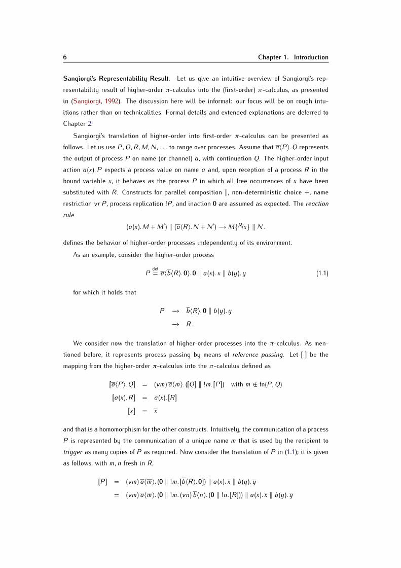
Sangiorgi’s Representability Result. Let us give an intuitive overview of Sangiorgi’s rep-resentability result of higher-order π-calculus into the (first-order) π-calculus, as presentedin (Sangiorgi, 1992). The discussion here will be informal: our focus will be on rough intu-itions rather than on technicalities. Formal details and extended explanations are deferred toChapter 2.Sangiorgi’s translation of higher-order into first-order π-calculus can be presented asfollows. Let us use P,Q, R,M,N, . . . to range over processes. Assume that a〈P〉.Q representsthe output of process P on name (or channel) a, with continuation Q. The higher-order inputaction a(x).P expects a process value on name a and, upon reception of a process R in thebound variable x, it behaves as the process P in which all free occurrences of x have beensubstituted with R . Constructs for parallel composition ‖, non-deterministic choice +, namerestriction νr P, process replication !P, and inaction 0 are assumed as expected. The reactionrule (a(x).M +M′) ‖ (a〈R〉.N +N′) −→ M{R/x} ‖ N .defines the behavior of higher-order processes independently of its environment.As an example, consider the higher-order process
P def= a〈b〈R〉. 0〉. 0 ‖ a(x). x ‖ b(y).y (1.1)for which it holds that
P −→ b〈R〉. 0 ‖ b(y).y−→ R .We consider now the translation of higher-order processes into the π-calculus. As men-tioned before, it represents process passing by means of reference passing. Let [[·]] be themapping from the higher-order π-calculus into the π-calculus defined as
[[a〈P〉.Q]] = (νm)a〈m〉. ([[Q]] ‖ !m. [[P]]) with m /∈ fn(P,Q)[[a(x).R ]] = a(x). [[R ]][[x]] = xand that is a homomorphism for the other constructs. Intuitively, the communication of a processP is represented by the communication of a unique name m that is used by the recipient totrigger as many copies of P as required. Now consider the translation of P in (1.1); it is givenas follows, with m,n fresh in R ,
[[P]] = (νm)a〈m〉. (0 ‖ !m. [[b〈R〉. 0]]) ‖ a(x). x ‖ b(y).y= (νm)a〈m〉. (0 ‖ !m. (νn)b〈n〉. (0 ‖ !n. [[R ]])) ‖ a(x). x ‖ b(y).y
1.2. First-Order and Higher-Order Concurrency 7
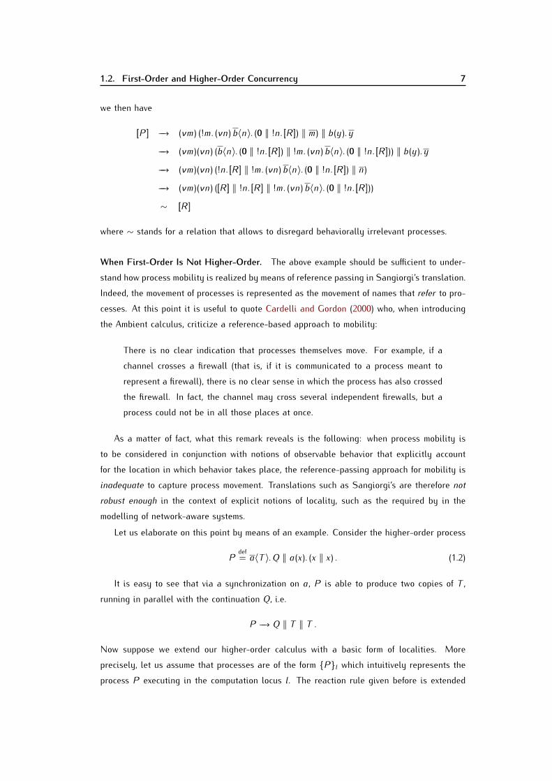
we then have[[P]] −→ (νm) (!m. (νn)b〈n〉. (0 ‖ !n. [[R ]]) ‖ m) ‖ b(y).y−→ (νm)(νn) (b〈n〉. (0 ‖ !n. [[R ]]) ‖ !m. (νn)b〈n〉. (0 ‖ !n. [[R ]])) ‖ b(y).y−→ (νm)(νn) (!n. [[R ]] ‖ !m. (νn)b〈n〉. (0 ‖ !n. [[R ]]) ‖ n)−→ (νm)(νn) ([[R ]] ‖ !n. [[R ]] ‖ !m. (νn)b〈n〉. (0 ‖ !n. [[R ]]))∼ [[R ]]
where ∼ stands for a relation that allows to disregard behaviorally irrelevant processes.When First-Order Is Not Higher-Order. The above example should be sufficient to under-stand how process mobility is realized by means of reference passing in Sangiorgi’s translation.Indeed, the movement of processes is represented as the movement of names that refer to pro-cesses. At this point it is useful to quote Cardelli and Gordon (2000) who, when introducingthe Ambient calculus, criticize a reference-based approach to mobility:
There is no clear indication that processes themselves move. For example, if achannel crosses a firewall (that is, if it is communicated to a process meant torepresent a firewall), there is no clear sense in which the process has also crossedthe firewall. In fact, the channel may cross several independent firewalls, but aprocess could not be in all those places at once.As a matter of fact, what this remark reveals is the following: when process mobility isto be considered in conjunction with notions of observable behavior that explicitly accountfor the location in which behavior takes place, the reference-passing approach for mobility isinadequate to capture process movement. Translations such as Sangiorgi’s are therefore notrobust enough in the context of explicit notions of locality, such as the required by in themodelling of network-aware systems.Let us elaborate on this point by means of an example. Consider the higher-order process
P def= a〈T 〉.Q ‖ a(x). (x ‖ x) . (1.2)It is easy to see that via a synchronization on a, P is able to produce two copies of T ,running in parallel with the continuation Q, i.e.
P −→ Q ‖ T ‖ T .Now suppose we extend our higher-order calculus with a basic form of localities. Moreprecisely, let us assume that processes are of the form {P}l which intuitively represents theprocess P executing in the computation locus l. The reaction rule given before is extended

8 Chapter 1. Introduction
accordingly; it allows interactions between complementary actions in two possibly differentlocalities: {a(x).M +M′}m ‖ {a〈R〉.N +N′}n −→ {M{R/x}}m ‖ {N}n .Let us consider P ′, the located version of P in (1.2). Process P ′ involves two differentlocalities s and r for sender and receiver processes, respectively:
P ′ def= {a〈T 〉.Q}s ‖ {a(x). (x ‖ x)}r .The behavior of P ′ is essentially the same of P, except for the fact that T is associated tolocation r. Intuitively, this represents the movement of T in the space of locations both s andr belong to: P ′ −→ {Q}s ‖ {T ‖ T}r .Indeed, we now have an observable behavior of the system that is finer in that we are nowable to tell not only that Q executes in parallel with two copies of T , but also that Q executesin location s whereas that T ‖ T executes in location r. Let us consider the first-orderrepresentation of P ′ given by the extension of Sangiorgi’s translation to the located case.(Without loss of generality we can assume that the translation [[·]] is homomorphic also withrespect to locations, i.e. [[{P}l]] = {[[P]]}l.) This way, we have
[[P ′]] = {(νm)a〈m〉. ([[Q]] ‖ !m. [[T ]])}s ‖ {a(x). (x ‖ x)}r−→ (νm) ({[[Q]] ‖ !m. [[T ]]}s ‖ {m ‖ m}r)−→ (νm) ({[[Q]] ‖ [[T ]] ‖ !m. [[T ]]}s ‖ {m}r)−→∼ {[[Q]] ‖ [[T ]] ‖ [[T ]]}s ‖ {0}rwhich is certainly unsatisfactory under any reasonable notion of behavioral equivalence withexplicit locations since, unlike the source term, process [[T ‖ T ]] is executed in location s. It isclear that what moved in the translation was a pointer to the copies, rather than the processesthemselves.The morale of this example is that while translations such as Sangiorgi’s are satisfactoryin the case of “basic” higher-order languages, this is not necessarily the case for higher-orderprocess calculi with specialized constructs, such as the ones required in global and ubiquitouscomputing scenarios. It is in this sense that we claim that Sangiorgi’s representability resultinduced a generalized misconception, both on the nature of higher-order communication andon the applicability of the translation. This is certainly not an original insight; as a matterof fact, Sangiorgi and Walker (2001) comment on this issue, remarking on the potentiallydangerous effects some other operators could have in Sangiorgi’s translation. Vivas and Dam(1998) and Vivas and Yoshida (2002) have studied such effects in the case of higher-order lan-guages involving dynamic binding. Also, the nature of the passivation operators introduced in

1.3. This Dissertation 9
(Hildebrandt et al., 2004; Schmitt and Stefani, 2004) to represent the suspension of executingprocesses as required in, e.g., forms of dynamic system reconfiguration strongly suggeststhat they are not representable into some first-order setting. All these works thus provide com-pelling evidence of the need of developing the theory of higher-order process calculi directlyon them, without going through intermediate translations.1.3 This Dissertation
This dissertation studies expressiveness and decidability issues in higher-order concurrency.The research is centered around a core calculus for higher-order concurrency in which onlythe operators strictly necessary to obtain higher-order communication are retained. Next, wegive an overview to expressiveness and decidability in concurrent languages in general, andin higher-order concurrency in particular. Then, we elaborate on the approach we shall followin our research. Finally, we comment on the contributions and structure of the dissertation.1.3.1 Expressiveness and Decidability in Higher-Order Concurrency
An important criterion for assessing the significance of a paradigm is its expressiveness. Ex-pressiveness studies are concerned with formal assessments of the expressive power of alanguage or family of languages. The precise meaning of “expressive power” depends on thepurpose, and several suitable definitions are possible. At the heart of all of them, however,is the notion of encoding: a map from the terms of a source language into those of a targetlanguage, subject to a set of correctness criteria.The quest for a unified definition of encoding in particular, a set of correctness criteriathat a good encoding should enforce has been a matter of research for some time now, andconcrete proposals have been put forward. In spite of this, there is yet no general agreementon such a definition. In our view, a single, all-embracing definition of encoding is unlikely toexist, essentially because expressiveness studies may have many different purposes, and maybe carried out over concurrent languages of a very diverse nature. This way, the set of criteriarequired in the definition of a taxonomy aimed at relating different process calculi should bedifferent from, for instance, the criteria required when the interest is on transferring reasoningprinciples from one language to another. Indeed, whereas in the latter case the definition ofencoding should impose rather strict criteria on the relationship between equivalent terms inboth source and target languages, in the former case the adopted definition could well enforcemilder forms of correspondence between equivalent terms, and/or consider criteria orientedat capturing precise aspects of the relationships of interest. Hence, differences between thetwo sets of criteria do not mean one is better than the other; they just reflect the differentmotivations underlying the respective expressiveness studies. Nevertheless, considering the
10 Chapter 1. Introduction
“quality” of an encoding is still interesting because, as we shall see, there is a direct relation-ship between the precise definition of encoding and the significance of the results obtainedwith it. We treat this issue in length in Chapter 2.As hinted at above, expressiveness has been little studied for higher-order process calculi.Most previous works address issues of relative expressiveness: higher-order calculi (both se-quential and concurrent) have been compared with first-order calculi, but mainly as a way ofinvestigating the expressiveness of the π-calculus and similar formalisms. In addition to therepresentability result in (Sangiorgi, 1992), the expressiveness of higher-order process calculiwas studied in (Sangiorgi, 1996b), where variants of the π-calculus with different degrees ofinternal mobility are related to typed variants of the Higher-Order π-calculus. Interestingly,this work presents encodings of (variants of) the π-calculus into strictly higher-order processcalculi, i.e., calculi in which only pure process passing is allowed and no name-passing ispresent. The only other result on the expressiveness of pure process passing we are aware ofis (Bundgaard et al., 2006), where an encoding of the π-calculus into Homer a higher-orderprocess calculi with locations (Hildebrandt et al., 2004) is presented. Encodings of variantsof the π-calculus into the Higher-Order π-calculus were first given in (Sangiorgi, 1996b) andlater consolidated in (Sangiorgi and Walker, 2001), where the abstraction mechanism of thehigher-order π-calculus is exploited. Thomsen (1990) and Xu (2007) have proposed encod-ings of π-calculus into Plain CHOCS. These encodings make essential use of the relabelingoperator of Plain CHOCS.The expressiveness of concurrent languages is closely related to decidability issues. Givena concurrent language, it is legitimate to ask whether or not its expressive power is related tothe decidability of some property of interest. Examples include properties related with behav-ioral equivalences (e.g. strong bisimilarity), termination of processes (e.g. convergence), andgraph-like structures (e.g. reachability and coverability). An appealing question here is “whatis the most expressive fragment of the language in which the property is decidable?” There isa trade-off between expressiveness and decidability: most interesting decision problems aregenerally undecidable for very expressive languages. Hence, given a process calculus andsome property of interest, a common research direction is identifying the largest sub-calculusfor which the property is decidable. Studies dealing with the interplay of expressiveness anddecidability are relevant in that they provide support for verification: they might pave the wayfor the implementation of tools, or provide insights on the aspects that might be sensible forverification purposes.Studies of decidable properties for higher-order process calculi are scarce. The only workwe are aware of is (Bundgaard et al., 2009), in which the interest is on the decidability ofbarbed bisimilarity in the context of Homer.
1.3. This Dissertation 11
1.3.2 Approach
We shall follow a direct and minimal approach for investigating the expressive power anddecidability of higher-order process calculi.Our approach is direct in that we abandon the idea of studying the foundations of higher-order concurrency by means of translations into first-order languages. Based on the inade-quacy of studying higher-order concurrency through first-order translations (as discussed inthe previous section), we advocate that foundational studies for higher-order process calculimust be carried out directly on them and exploit their peculiarities. While we concentrateon expressiveness and decidability issues, this direct approach is in concordance with thatadvocated by recent works on other aspects of the theory of higher-order process calculi, suchas behavioral theory (see, e.g., (Lenglet et al., 2008; Sato and Sumii, 2009)) and type systems(Demangeon et al., 2010).On the other hand, our approach is minimal in that the research shall be centered arounda core calculus for higher-order concurrency in which only the operators strictly necessary toobtain higher-order communication are retained. The calculus, called HOCORE, aims to be thesimplest, non-trivial process calculus featuring higher-order concurrency. In particular:• HOCORE has no name-passing, so processes are the only kind of values that can bepassed around in communications. This is in sharp contrast to most higher-order processcalculi in the literature, in which both name-passing and process-passing are present.• HOCORE has no restriction operator, thus all channels are global, and dynamic creationof new channels is impossible. As such, the behavior of a concurrent system describedin HOCORE is completely exposed. Also, it is worth noticing that the syntax of higher-order process calculi (including HOCORE) usually omits primitive operators for infinitebehavior (as replication), as they can be encoded by mimicking the structure of fixed-point combinators in the λ-calculus. Known encodings of fixed-point combinators requirerestriction; therefore, the lack of restriction in HOCORE is directly related to its abilityof expressing infinite behavior. While in most of the dissertation we consider HOCORE(or variants of it) without restriction, we shall find it useful to consider an extension withrestriction useful when examining synchronous and polyadic communication.• HOCORE has no output prefix so it is an asynchronous calculus. It is well-known thatasynchronous communication is easier to implement and maintain that synchronous com-munication. As such, it appears as the most elemental communication discipline onecould adopt. Asynchrony represented as the absence of continuations after output ac-tions is the main feature of the asynchronous π-calculus, which was proposed in seminalpapers by Boudol (1992) and Honda and Tokoro (1991), and thoroughly studied since

12 Chapter 1. Introduction
then. Within concurrency theory, the expressive power of asynchrony has been stud-ied by Palamidessi (2003) (see also (Cacciagrano et al., 2007; Beauxis et al., 2008)),who showed that in the π-calculus with choice synchronous communication is more ex-pressive than asynchronous one. Even if the same phenomenon should not necessarilycarry over to a higher-order setting we shall address this issue in this dissertation, Palamidessi’s result ought be taken as an additional evidence of the simplicity thatasynchrony might embody in process calculi.The minimality of HOCORE is convenient in that it allows us to focus on higher-ordercommunication and its associated phenomena, without being shadowed by complex constructsnor by first-order interactions; studies of expressiveness and decidability for HOCORE willtherefore reflect the inherent to pure process passing and shed light on their intrinsic nature.
1.3.3 Contributions and Structure
The dissertation contributes to the theory of higher-order concurrency with several originalresults on the expressiveness and decidability of HOCORE and a number of selected variantsof it. Our results complement the few ones in the literature, and deepen and strengthen ourunderstanding of the theory core higher-order process calculi as a whole. More precisely, ourcontributions are structured as follows.Chapter 2: Preliminaries. This chapter provides the theoretical background for the thesis.We introduce fundamental concepts on process calculi, higher-order process calculi, andexpressiveness of concurrent languages.Chapter 3: HOCORE and its Expressiveness. We introduce HOCORE, a core calculus for high-er-order concurrency. We study the expressive power by encoding basic forms of choiceand input-guarded replication. Such derived constructs are then used to define an en-coding of Minsky machines into HOCORE, which demonstrates that the language is Turingcomplete. The encoding is deterministic and termination preserving; as such, propertiessuch as termination (i.e. the absence of divergent computation) and convergence (i.e. theexistence of a non-diverging computation) are immediately shown to be undecidable.Chapter 4: Behavioral Theory of HOCORE. We show that in HOCORE strong bisimilarity isdecidable. To the best of our knowledge, HOCORE is the first concurrent formalism that isTuring complete and for which bisimilarity is decidable. Furthermore, strong bisimilarityis shown to be a congruence, and to coincide with other well-established behavioralequivalences for higher-order calculi. A sound and complete axiomatization of strongbisimilarity is given, and used to obtain complexity bounds for bisimilarity checking. Thelimits of decidability are explored by considering an extension of HOCORE with static

1.3. This Dissertation 13
(top-level) restrictions. For the extension with four of such restrictions, bisimilarity isshown to be undecidable. This result is obtained through an encoding of the Postcorrespondence problem (PCP).Chapter 5: Expressiveness of Forwarding and Suspension. We study HO−f , the fragment ofHOCORE that results from forbidding nested output actions in communication objects.This represents a limitation of the forwarding capabilities of HOCORE. The expressivenessof HO−f is analyzed using decidability of termination and convergence as a yardstick.As in HOCORE, in HO−f convergence is still undecidable, a result obtained by exhibitingan unfaithful encoding of Minsky machines. In contrast, termination is shown to bedecidable. This result is obtained by appealing to the theory of well-structured transitionsystems. To the best of our knowledge, this is the first time such a theory is used in thehigher-order setting.
Decidability of termination suggests a loss of expressive power when passing fromHOCORE to HO−f . Then, as a way of recovering such power, we consider HOP−f , theextension of HO−f with a passivation construct that allows for process suspension at runtime. We show that in HOP−f , a faithful encoding of Minsky machines becomes possible.This implies that in HOP−f both convergence and termination are undecidable. To thebest of our knowledge, ours is the first result on the expressiveness and decidability ofpassivation operators in the higher-order setting.Chapter 6: Expressiveness of Synchronous and Polyadic Communication. We study the ex-pressive power of extensions of HOCORE with restriction. We call such an extensionAHO. As a first encodability result, we show that AHO is expressive enough to encodesynchronous communication. We then move to study the expressiveness of SHOn, theextension of HOCORE with name restriction, synchronous communication, and polyadiccommunication of arity n. We consider the family of higher-order process calculi given byvarying the polyadicity of such an extension. The main result is that polyadicity inducesa hierarchy of strictly increasing expressiveness: polyadic communication of arity n (asin SHOn) cannot be encoded into polyadic communication of arity n−1 (as in SHOn−1).Furthermore, we show that SHOna the extension of SHOn with abstraction-passingcannot be encoded into SHOn.Chapter 7: Conclusions and Perspectives. We draw conclusions from the research and dis-cuss perspectives of future work.
The calculi studied in the dissertation are depicted in Figure 1.1.Origin of the Chapters. Most of the material in this dissertation has been previously pre-sented in international conferences and appear in the respective proceedings. Even if many

14 Chapter 1. Introduction
HOcore
Ho−f
SHOn
HoP−f
AHOn
SHOna
HOcore +static restriction
Figure 1.1: The higher-order process calculi studied in this dissertation. An arrow indicateslanguage inclusion.improvements have been made with respect to the published material, we think that the basicideas behind the results remain the same.
• HOCORE and its behavioral theory as presented in Chapters 3 and 4 has been publishedas the paper (Lanese et al., 2008).• The expressiveness of forwarding in HOCORE, as presented in Chapter 5, is based onresults first published in the paper (Di Giusto et al., 2009a).• The expressiveness of polyadic communication as discussed in Chapter 6 is based onresults published as the extended abstract (Lanese et al., 2009).There are some results original to this dissertation; this unpublished material will beexplicitly mentioned in the corresponding chapter.
Chapter 2
Preliminaries
This chapter provides the theoretical background for the dissertation. It is in three sections. InSection 2.1 we introduce the basic terminology and concepts used in the dissertation. In orderto do so, we present a description of CCS (Milner, 1989) and of the π-calculus (Milner et al.,1992). In Section 2.2 we introduce higher-order process calculi: we review their origins andbehavioral theory. The higher-order π-calculus, as well as Sangiorgi’s representability result,are detailed there. Section 2.3 introduces main issues in the analysis of the expressivenessof concurrent languages. We give an overview to the most common kinds of expressivenessstudies and the techniques used to carry them out. Furthermore, previous efforts on studyingthe expressiveness of higher-order languages are reviewed.2.1 Technical Background
2.1.1 Bisimilarity
Broadly speaking, behavioral equivalences allow to determine when the behavior of two con-current system can be considered as equal. There are many plausible motivations for aimingat definitions of behavioral equivalences. For instance, one would like the behavior of theimplementation of system to be behaviorally equivalent to that of its specification; similarly,in a component-based system it is generally desirable to replace a component with a newone that features at least the same possibilities for behavior. Accordingly, many definitions ofbehavioral equivalences for concurrent systems have been proposed; notable notions includetrace equivalence which equates two processes if they can perform the same finite sequencesof transitions and the testing framework (De Nicola and Hennessy, 1984), in which the be-havior of two processes is deemed as equal if they pass the same tests provided by an externalobserver. In this context, bisimilarity is widely accepted as the finest behavioral equivalence

16 Chapter 2. Preliminaries
one would like to impose on processes. Following (Sangiorgi, 2009), we now define bisimilarityand state a few of its fundamental properties.A fundamental notion is that of Labeled Transition System (LTS in the sequel).Definition 2.1. A Labelled Transition System (LTS) is a triple (S, T , { t−→: t ∈ T}) where Sis a set of states, T is a set of (transition) labels, and t−→⊆ S × S for each t ∈ T is thetransition relation.
It is customary to write P α−−→ Q to denote the fact that (P,Q) ⊆ α−−→. In the contextof concurrency theory, it is natural to relate states and processes, and labels as the actionsprocesses can perform. This way, P α−−→ Q is indeed a transition which represents that processP can perform α and evolve into Q. The transition relation for a process language is generallydefined by means of a set of transition rules which realize the intended behavior of eachconstruct of the language. In what follows, we say that a process relation is a binary relationon the states of an LTS.Definition 2.2 (Bisimilarity). A process relation R is a bisimulation if, whenever PRQ, for allα we have that:
1. for all P ′ with P α−−→ P ′, there is Q′ such that Q α−−→ Q′ and P ′RQ′;2. the converse, on the transitions emanating from Q: for all Q′ with Q α−−→ Q′, there is P ′such that P α−−→ P ′ and P ′RQ′.
Bisimilarity, written ∼, is the union of all bisimulations; thus P ∼ Q if there is a bisimulationR with PRQ.Given this definition, the bisimulation proof method naturally follows: to determine thattwo processes P and Q are bisimilar, it is sufficient to exhibit a bisimulation relation containing(P,Q). It is useful to state a few fundamental properties of bisimilarity.
Theorem 2.1 (Basic Properties of Bisimilarity). Given ∼, it holds that:1. ∼ is an equivalence relation, i.e., it is reflexive, symmetric, and transitive.2. ∼ is itself a bisimulation.Item (2) is insightful in that it allows to grasp the circular flavor of bisimilarity: bisimilarityitself is a bisimulation, and is part of the union on which it is defined. Hence, the followingtheorem holds.
Theorem 2.2. Bisimilarity is the largest bisimulation.

2.1. Technical Background 17
2.1.2 A Calculus of Communicating Systems
We introduce a number of relevant concepts of CCS, following the presentation in Milner(1989).CCS departs from theories of sequential computation by focusing on the notion of inter-action: a concurrent system interacts with its environment which realizes the behavior of thesystem through observations. In CCS like in other process calculi such as ACP and CSPthe overall behavior of a system is entirely determined by the atomic actions it performs. Thedistinguishing principle in CCS is that the notion of interaction is equated to that of obser-vation: not only actions are observable, but we observe an action produced by the system byinteracting with it, that is, by performing its complementary action, or coaction. We then saythat the two participants, system and observer, have synchronized in the action by means ofthis mutual observation.
Syntax. We shall assume a set of names N = {a, b, c, . . .}, as well as a disjoint set ofco-names defined as N = {a | a ∈ N}. There is a set of labels defined as L = N ∪ N ;we let l, l′, . . . range over L. Labels give an account of the observable behavior of the system.We shall use K, L for subsets of L; L stands for the set of complements of the labels in L.We consider the distinguished symbol τ representing the internal or silent action that resultsfrom synchronizations. We then define A = L ∪ τ to be the set of actions; α, β range overA. In the spirit of the above discussion, actions a and a are thought of as complementary;this way, a = a and τ = τ. The set of CCS processes expressing finite behavior is given asfollows:Definition 2.3. The set of finite CCS processes is given by the following syntax:
P,Q, . . . ::= ∑i∈I αi.Pi | P\a | P1 ‖ P2
where I is an indexing set.The summation ∑i∈I αi.Pi represents the process that is able to perform one and only oneof its actions αi, and then behaves as its associated Pi. It is customary to write 0 nil, theprocess that does nothing in case | I |= 0, α .P if | I |= 1, and “+” for binary sum. Therestriction P\a behaves exactly as P but it cannot offer neither a or a to its surroundingenvironment. Both a and a are then said to be bound in P; we shall use fn(P) to denote theset of free names, i.e., not bound, in P; the bound names of P, bn(P), are those with a boundoccurrence in P. The parallel composition P ‖ Q allows P and Q to run concurrently: eitherP or Q may perform an action, or they can synchronize by performing complementary actions.

18 Chapter 2. Preliminaries
SUM ∑i∈I αi.Pi αj−→ Pj if j ∈ I RES P α−→ P ′P\a α−→ P\a if a /∈ {α, α }PAR1 P α−→ P ′P ‖ Q α−→ P ′ ‖ Q TAU P l−→ P ′ Q l−→ Q′P ‖ Q τ−→ P ′ ‖ Q′
Figure 2.1: An LTS for CCS. Rule PAR2, the symmetric of PAR1, is omitted.Semantics and Infinite Behavior. The operational semantics of CCS is given by an LTS inwhich the set of processes is the set of states, and the set of labels is taken to be A, the setof actions in CCS. The transition relation is given by the set of transition rules in Figure 2.1.Let us move now to the different ways of expressing infinite behavior. We consider recursionand replication. In order to represent recursion a denumerable set of constants, ranged over byD, is assumed. It is also assumed that each constant D has associated a (possibly recursive)defining equation of the form D def= P. The extension of (finite) CCS with recursion is then isobtained by adding the production P ::= D to the grammar in Definition 2.3, and by extendingthe operational semantics in Figure 2.1 with the following transition rule
CONS P α−→ P ′ D def= PD α−→ P ′ .As Busi et al. (2009) remark, recursive behavior defined by means of constants can beintuitively assimilated to infinite behavior “in depth”, in that process copies can be nestedat an arbitrary depth by using constant application. This is in sharp contrast to the kindof infinite behavior provided by replication: by means of the replication operator !P it ispossible to obtain an unbounded number of copies of P; such copies, however, are all atthe same level, thus defining infinite behavior “in width”. The extension of (finite) CCS withreplication is obtained by adding the production P ::= !P to the grammar in Definition 2.3,and by extending the operational semantics in Figure 2.1 with the following transition rule
REPL P ‖ !P α−→ P ′!P α−→ P ′ .A word on proof techniques is most convenient at this point. Defining the semantics interms of a LTS provides us automatically with two basic proof techniques, both of which areforms of induction: one on the structure of process terms (structural induction), and one on thetransition rules (transition induction). The finitary character of inductive proof techniques isin contrast with the infinite behavior concurrent systems generally exhibit. As a result, whenaddressing the issue of equality of concurrent systems, one needs to appeal to coinductive prooftechniques. Bisimilarity as introduced in Section 2.1.1, is probably the most representativecoinductive proof-technique.

2.1. Technical Background 19
2.1.3 More on Behavioral Equivalences
Having introduced the notion of bisimilarity, and some basic notions of CCS, we find it useful toinformally present some additional concepts on behavioral equivalences. The discussion hereis intended to introduce useful terminology; technical accounts of the concepts mentioned herecan be found elsewhere (see, e.g., (Sangiorgi, 2009; Milner, 1989)).It is desirable to require bisimilarity to be preserved by all process contexts. This allowsto replace, in any process expression, a subterm with a bisimilar one. An equivalence relationwith this property is said to be a congruence. Proofs of congruence combine inductive andcoinductive arguments: the former are necessary as the syntax of the processes is definedinductively, whereas the latter are required in that bisimilarity is a coinductive definition. Inthe case of CCS we have the following.Theorem 2.3. In CCS, ∼ is a congruence relation.
When bisimilarity is decidable, it may be possible to give an algebraic characterization of it,or axiomatization. The axiomatization of an equivalence on a set of terms consists essentiallyof some equational axioms that suffice for proving all and only the equations among theterms that are valid for the given equivalence. These axioms are used together with rules ofequational reasoning, which include reflexivity, symmetry, transitivity, and congruence rulesthat allow to replace any subterm of a process with an equivalent one. A bit more formally,given a set of axioms S, it is usual to write S ` P = Q if one can derive P = Q using theaxioms in S and the laws of equational reasoning. The objective is then to show that theaxiomatization is a full characterization of bisimilarity, i.e., that it is both sound and completewith respect to bisimilarity:P ∼ Q if and only if S ` P = Q . (2.1)
While establishing soundness (i.e., the backward direction in (2.1)) is in general easy,establishing completeness (i.e., the forward direction in (2.1)) often involves defining somestandard syntactic form for processes and requires more effort. This the case of, e.g., finite-state CCS processes as studied by Milner (1989).We have seen that CCS considers the special action τ as a form of internal activity. Oftenit is useful to describe concurrent behavior by abstracting from such internal actions. Thisgives rise to weak transition relations, denoted =⇒ and α==⇒. While P =⇒ Q is used to meanthat P can evolve to Q by performing any number of internal actions (even zero), P α==⇒ Qmeans that P can evolve to Q as a result of an evolution that includes an action α , but mayinvolve any number of internal actions before and after α . As such, τ==⇒ is different from =⇒as the former guarantees that at least one internal action has been performed. More formally,we have the following.

20 Chapter 2. Preliminaries
Definition 2.4 (Weak transitions). .• Relation =⇒ is the reflexive and transitive closure of τ−−→. That is, P =⇒ P ′ holds if thereif there is n ≥ 0 and processes P1, . . . , Pn with Pn = P ′ such that P τ−−→ P1 · · · τ−−→ Pn.(Notice that P =⇒ P holds for all processes.)• For all α ∈ T , relation α==⇒ is the composition of the relations =⇒, α−−→, and =⇒. Thatis, P α==⇒ P ′ holds if there are P1, P2 such that P =⇒ P1 α−−→ P2 =⇒ P ′.With the aid of weak transitions, it is possible to define weak bisimulation and weakbisimilarity, as in the following definition.
Definition 2.5. A process relation R is a weak bisimulation if, whenever PRQ, for all α wehave:1. for all P ′ with P α==⇒ P ′ there is a Q′ such that Q α==⇒ Q′ and P ′RQ′;2. for all P ′ with P τ==⇒ P ′ there is a Q′ such that Q =⇒ Q′ and P ′RQ′;3. the converse of (1) and (2), on the actions from Q.
P and Q are weakly bisimilar, written P ≈ Q, if PRQ for some weak bisimulation R.We now discuss the ideas behind barbed bisimilarity (Milner and Sangiorgi, 1992). Atransition P α−−→ P ′ of an LTS intuitively describes a pure synchronization between P and itsexternal environment along a port a mentioned in α . This is but one particular of concurrentinteraction; a natural question that arises is how to adapt the idea of bisimulation to otherkinds of interaction. The idea is to set a bisimulation in which the observer has a minimalability to observe actions and/or process states. This yields a bisimilarity, namely indistin-guishability under such observations, which in turns yields a congruence over terms, namelybisimilarity in all contexts. The bisimilarity is called barbed bisimilarity; the congruence iscalled barbed congruence.The main assumption in the barbed setting is the existence of a reduction relation in thelanguage. Such a relation is intended to express an evolution step of a term in which nointervention from the environment is required. In CCS, such a relation is τ−−→. The reductionrelation represents the most fundamental notion in the operational semantics of a language.The reduction semantics of a language is then an approach to operational semantics in whichthe meaning is only attached to reductions; it explains how a system can evolve independentlyof its environment. This approach is then in clear contrast to that underlying a labeledtransition system.In barbed bisimilarity the clauses involve challenges only on reductions. In addition, equalprocesses should exhibit the same barbsi.e., predicates representing basic observables of

2.1. Technical Background 21
the states. Barbs are of the essence to obtain an adequate discriminating power. Barbedcongruence is a contextual equivalence: it is the closure of barbed bisimilarity over contexts.The definition of barbs we shall be interested in is as follows.Definition 2.6. Given a visible action α , the observability predicate ↓α holds for a process Pif, for some P ′, P α−−→ P ′.
We now define strong barbed bisimulation.Definition 2.7 (Barbed bisimilarity). A process relation R is said to be a barbed bisimulationif whenever P .∼ Q it implies:
1. whenever P −→ P ′ then Q −→ Q′ and P ′RQ′;2. for each visible action α , if P ↓α then P ↓α .
Barbed bisimilarity, written .∼, is the union of all barbed bisimulations.The weak version of Definition 2.7 is obtained in the standard way. Let =⇒ be the reflexiveand transitive closure of −→ and ⇓a be defined as =⇒↓a. Then, weak barbed bisimulation,written .≈, is defined by replacing the reduction Q =⇒ Q′ with Q =⇒ Q′ and the predicate Q ↓µwith Q ⇓ µ. As mentioned before, by quantifying over contexts, we obtain barbed congruence:
Definition 2.8. Two processes P and Q are said to be strongly barbed congruent, writtenP ' Q, if for every context C [·], it holds that C [P] .∼ C [Q].We obtain weak barbed congruence, written ∼=c, by replacing .∼ with .≈ in the definitionabove.A main drawback of the notion of barbed congruence is that the universal quantification oncontexts, which can make it impractical to use in proofs. The challenge is then to find tractablecharacterizations of barbed congruence. A well-established approach here is to use (labeled)bisimilarities: the objective is to find a bisimilarity that is both sound and complete withrespect to barbed congruence. That is, a notion of bisimilarity that both includes and containsbarbed congruence. While for the case of CCS and the π-calculus effective characterizationsof barbed congruence have been thoroughly studied (see, e.g., (Sangiorgi and Walker, 2001)),we shall see that this is not quite the case for higher-order process calculi, in which thesituation is much less clear.
2.1.4 A Calculus of Mobile Processes
We introduce the (polyadic) π-calculus following the presentation given in (Sangiorgi, 1992,1993); this will make the introduction of the higher-order π-calculus easier. The reader is

22 Chapter 2. Preliminaries
referred to (Milner et al., 1992; Sangiorgi and Walker, 2001) for complete references on theπ-calculus.The π-calculus departs from CCS with the capability of sending (first-order) values alongcommunication channels. Its significance derives from the fact that such values include theset of communication channels; new communication channels can be created dynamically, andshared among processes, possibly in a restricted way. This is most useful to represent dynamiccommunication topologies.Syntax. We use a, b, c, . . . , x, y, z, . . . to range over names (or channels) and P,Q, R, T , . . .to range over processes. We use a tilde to represent tuples of elements; this way, given a namey, y stands for a tuple of names. The set of π-calculus processes is given by the followingdefinition.Definition 2.9. The set of π-calculus processes is given by the following syntax:
P,Q, . . . ::= ∑i∈I αi.Pi | P1 ‖ P2 | (νx)P | [x = y]P | D〈x〉
where I is any finite indexing set. The set of prefixes is given byα ::= x(y) | x〈y〉 .
As in CCS, we assume that each constant D has a defining equation of the form D def= (x)P,where the parameters x collect all names which may occur free in P. Some constraints totuples in input and output prefixes are in order. In an input prefix x(y), tuple y is required tobe made of pairwise distinct elements. We omit brackets ( ) and 〈 〉 when the tuple is empty.Also, tuple y is required to be finite in both input and output prefixes. This is not the case forthe tuple x in constant definitions and applications; hence, it can be infinite.The intuitive semantics of processes is as expected. An input-prefixed process x(y).P waitsfor a tuple z to be transmitted along name x; once this occurs, the process P in which y hasbeen instantiated by z executes. An output-prefixed process x〈y〉.P sends tuple y along xand then behaves like P. The matching operator [x = y]P is used to test for equality of thenames x and y. The intuition behind the restriction operator is somewhat similar to that inCCS: (νx)P makes name x local to P; thus x becomes a new, unique name, distinct from allthose external to P. We often write (νx)P to stand for the process (νx1)(νx2) . . . (νxn)P. Thesemantics and notation for (guarded) summation follow those in CCS. In particular, we shalluse + to represent binary sum.We have already commented on the use of constants to represent infinite behavior. Noticethat it is possible to encode replication using constants. It is worth noticing that, givenD = 〈x〉P, in an application D(y) tuple y must be of the same length as x. This kind of

2.1. Technical Background 23
potential disagreements on the arities of tuples, as well as some other aspects of the name-passing discipline, are enforced by the use of appropriate type systems on names.1 For thesake of conciseness, we do not elaborate on the definitions and properties of sorts. As such,along the chapter we always assume well-sorted processes; we use notation x : y to meanthat names x and y have the same sort. If D def= (x)P and x is not empty then D and (x)P arecalled abstractions. Abstractions and processes are agents. We use F, E, . . . and A to rangeover abstractions and agents, respectively.Notions of free and bound names are as expected: in a(b).P, (νb)P, and (b)P all freeoccurrences of names b in P are bound. The sets of free and bound names of an agent A aredenoted fn(A) and bn(A), respectively. Notice that if A = D〈x〉 then fn(A) = x and bn(A) = ∅.Name substitution is a function from names to names. Given a vector of distinct names x, wewrite {y/x} for the substitution that maps the xi-th name in x to the yi-th name in y, andmaps all names not in x to themselves. We assume standard definitions of substitution andα-conversion on processes, with possible renamings so as to avoid capture of free names. Inwhat follows we shall be working modulo α-conversion, and hence we decree two processesas equal if one is α-convertible into the other.Operational Semantics. We present now a reduction semantics and an LTS for the π-calculus. As argued before, the reduction semantics is intended to capture the behavior thatis intrinsic to a process, that is, the behavior that does not include the potential interactionsbetween the process and its environment. Central to the reduction semantics is the notionof structural congruence that allows flexibility in the syntactic structure of the process, thuspromoting interactions to occur.Structural congruence, denoted ≡, is the smallest congruence over the set of π-calculusprocesses that satisfies the following rules:
1. P ≡ Q if P is α-convertible to Q;2. abelian monoid laws for +: P + 0 ≡ P, P +Q ≡ Q + P, (P +Q) + R ≡ P + (Q + R);3. abelian monoid laws for ‖: P ‖ 0 ≡ P, P ‖ Q ≡ Q ‖ P, (P ‖ Q) ‖ R ≡ P ‖ (Q ‖ R);4. laws for restriction: νx0 ≡ 0, νx νyP ≡ νy νxP, (νxP) ‖ Q ≡ νx(P ‖ Q) if x 6∈ fn(Q);5. law for match: [x = x]P ≡ P;6. law for constants: if D def= (x)P and x : y then D〈y〉 ≡ P{y/x}. (In case of replication isused: !P ≡ P ‖ !P.)1In early proposals of the π-calculus (see, e.g., (Milner, 1991)) discipline on names was enforced by the notionof sorting. The presentation of the first- and higher-order π-calculus in (Sangiorgi, 1992) relies on sorts. In (Pierceand Sangiorgi, 1996) the notion of sort was refined into the notion of typing for processes.
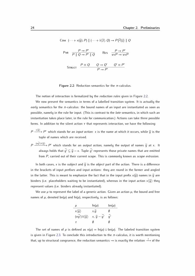
24 Chapter 2. Preliminaries
COM (· · ·+ x(y).P) ‖ (· · ·+ x〈z〉.Q) −→ P{z/y} ‖ QPAR P −→ P ′P ‖ Q −→ P ′ ‖ Q RES P −→ P ′νxP −→ νxP
STRUCT P ≡ Q Q −→ Q′ Q′ ≡ P ′P −→ P ′
Figure 2.2: Reduction semantics for the π-calculus.The notion of interaction is formalized by the reduction rules given in Figure 2.2.We now present the semantics in terms of a labelled transition system. It is actually theearly semantics for the π-calculus: the bound names of an input are instantiated as soon aspossible, namely in the rule for input. (This is contrast to the late semantics, in which such aninstantiation takes place later, in the rule for communication.) Actions can take three possibleforms. In addition to the silent action τ that represents interaction, we have the following:
P x〈y〉−−−→ P ′ which stands for an input action: x is the name at which it occurs, while y is thetuple of names which are received.P (νy′) x〈y〉−−−−−−→ P ′ which stands for an output action, namely the output of names y at x. Italways holds that y′ ⊆ y− x. Tuple y′ represents those private names that are emittedfrom P, carried out of their current scope. This is commonly known as scope extrusion.
In both cases, x is the subject and y is the object part of the action. There is a differencein the brackets of input prefixes and input actions: they are round in the former and angledin the latter. This is meant to emphasize the fact that in the input prefix x(y) names in y arebinders (i.e. placeholders waiting to be instantiated), whereas in the input action x〈y〉 theyrepresent values (i.e. binders already instantiated).We use µ to represent the label of a generic action. Given an action µ, the bound and freenames of µ, denoted bn(µ) and fn(µ), respectively, is as follows:µ fn(µ) bn(µ)x〈y〉 x,y ∅(νy′) x〈y〉 x, y− y′ y′τ ∅ ∅
The set of names of µ is defined as n(µ) = fn(µ) ∪ bn(µ). The labeled transition systemis given in Figure 2.3. To conclude this introduction to the π-calculus, it is worth mentioningthat, up to structural congruence, the reduction semantics −→ is exactly the relation τ−−→ of the

2.2. Higher-Order Process Calculi 25
ALP P ′ µ−→ Q P and P ′ are α-convertibleP µ−→ QINP x(y).P x〈z〉−−→ P{z/y}, if | z |=| y | OUT x〈y〉.P x〈y〉−−→ P
SUM P µ−→ P ′P +Q µ−→ P ′ PAR P µ−→ P ′P ‖ Q µ−→ P ′ ‖ Q bn(µ) ∩ fn(Q) = ∅COM P1 (νy′)x〈y〉−−−−−→ P ′ Q x〈y〉−−→ Q′ y′ ∩ fn(Q) = ∅P ‖ Q τ−→ νy′(P ′ ‖ Q′)
RES P µ−→ P ′ r 6∈ n(µ)νr P µ−→ νr P ′ CONST P{y/x} µ−→ P ′D〈y〉 µ−→ P ′ if D def= (x)POPEN P (νy′)z〈y〉−−−−−→ P ′νx P (νx,y′)z〈y〉−−−−−−→ P ′ x 6= z, x ∈ fn(y)− y′ MATCH P µ−→ P ′[x = x]P µ−→ P ′
Figure 2.3: The (early) labeled transition system for the π-calculus. Rules ACT2 and TAU2,the symmetric counterparts of rules ACT1 and TAU1, are omitted.labeled transition semantics. This result is sometimes referred to as the harmony lemma (see,e.g., Sangiorgi and Walker (2001)).2.2 Higher-Order Process Calculi
Higher-order process calculi are calculi in which processes (more generally, values containingprocesses) can be communicated. Thus a computation step involves the instantiation of avariable with a term, which is then copied as many times as there are occurrences of thevariable. If there are multiple occurrences, the size of a system may grow. Higher-orderprocess calculi have been put forward in the early 90s, with CHOCS (Thomsen, 1989) andPlain CHOCS (its variant with static binding) (Thomsen, 1990), and with the Higher-Orderπ-calculus (Sangiorgi, 1992). The basic operators are those of CCS (Milner, 1989).The appearance of processes inside values usually has strong consequences on the se-mantics: namely on labeled transition systems (notions of alpha conversion, higher-order sub-stitutions, scope extrusions) and, especially, on behavioral equivalences (e.g. bisimulation).Higher-order, or process-passing, concurrency is often presented as an alternative paradigmto the first order, or name-passing, concurrency of the π-calculus for the description of mo-bile systems, i.e. concurrent systems whose communication topology may change dynamically.Higher-order calculi are formally closer to the λ-calculus, whose basic computational step β-reduction involves term instantiation. As in the λ-calculus, a computational step inhigher-order calculi results in the instantiation of a variable with a term, which is then copied

26 Chapter 2. Preliminaries
as many times as there are occurrences of the variable, resulting in potentially larger terms.The remainder of this section is structured as follows. In Section 2.2.1 we present thehigher-order π-calculus; this is necessary to introduce Sangiorgi’s representability result inSection 2.2.2. Then, in Section 2.2.3 we review several proposals of higher-order languages inthe literature. Finally, in Section 2.2.4, we report on previous works on the behavioral theoryfor languages in the higher-order setting.2.2.1 The Higher-Order π-calculus
Here we present the higher-order π-calculus, abbreviated HOπ. We introduce the languageby building on the notations presented for the π-calculus in Section 2.1.4.Let Var be a set of agent-variables, ranged over X, Y . In order to obtain HOπ, the syntaxof the π-calculus (cf. Section 2.1.4) is modified in two ways. First, variable application isallowed, so that an abstraction received as input can be provided with appropriate arguments.Second, tuples in inputs, outputs, applications, and abstraction may also contain agent oragent-variables. To simplify the notation in the grammar below we use K to stand for anagent or a name and U to stand for a variable or a name.P,Q ::= ∑
i∈I αi.Pi | P ‖ Q | νxP | [x = y]P | D〈K 〉 | X〈K 〉α ::= x〈K 〉 | x(U)
Recall that K may be an agent: hence, it may be a process, but also an abstraction ofarbitrary high order. The grammar of agents is the following:A ::= (U)P | (U)X〈K 〉 | (U)D〈K 〉
(Notice also that a variable X and a constant D are agents, corresponding to the cases inwhich U and K are empty. We make the assumptions regarding finiteness of tuples as in theπ-calculus. A variable X which is not underneath some input prefix x(U) or an abstraction(U) with X ∈ U is said to be free. An agent containing free variables is said to be open. Weuse fv(A) to denote the set of free variables of agent A.In HOπ the notions of types and type systems are more involved than in the π-calculus.For the sake of conciseness, we do not present such details here, and assume well-sortedexpressions. The reader is referred to (Sangiorgi, 1992, 1996b) for details.Now we present reduction and labeled transition semantics for HOπ. Let us introduce thereduction semantics first. The structural congruence rules and the reduction rules for HOπare the same as for the π-calculus. We only have to generalize the structural congruence rule

2.2. Higher-Order Process Calculi 27
ALP P ′ µ−→ Q P and P ′ are α-convertibleP µ−→ QINP x(U).P x〈K 〉−−−→ P{K/U}, if | z |=| y | OUT x〈K 〉.P x〈K 〉−−−→ P
SUM P µ−→ P ′P +Q µ−→ P ′ PAR P µ−→ P ′P ‖ Q µ−→ P ′ ‖ Q bn(µ) ∩ fn(Q) = ∅COM P1 (νy)x〈K 〉−−−−−→ P ′ Q x〈K 〉−−→ Q′ y′ ∩ fn(Q) = ∅P ‖ Q τ−→ νy(P ′ ‖ Q′)
RES P µ−→ P ′ r 6∈ n(µ)νr P µ−→ νr P ′ CONST P{K/U} µ−→ P ′D〈K 〉 µ−→ P ′ if D def= (U)POPEN P (νy)z〈K 〉−−−−−→ P ′νx P (νx,y)z〈K 〉−−−−−−→ P ′ x 6= z, x ∈ fn(K )− y MATCH P µ−→ P ′[x = x]P µ−→ P ′
Figure 2.4: The labeled transition system for HOπ. Rules ACT2 and TAU2, the symmetriccounterparts of rules ACT1 and TAU1, are omitted.(6) and the rule COM, so that the tuples involved may contain agents. This way, these rulesbecome, respectively:
6. If D def= (U)P and U : K , then D〈K 〉 ≡ P{K/U}and
COM (· · ·+ x(U).P) ‖ (· · ·+ x〈K 〉) −→ P{K/U} ‖ Q .The labeled transition semantics for HOπ is given in Figure 2.4. It arises as a general-ization of that for the π-calculus given in Figure 2.3. While input actions take the form x〈K 〉,output actions are of the form (νy)x〈K 〉; for the latter it holds that y ⊆ fn(K )− x. The corre-spondence between reduction and labeled transition semantics mentioned for the π-calculusholds for HOπ as well.
2.2.2 Sangiorgi’s Representability Result
We now introduce C, the compilation of HOπ into the π-calculus, following the presentationin (Sangiorgi, 1993). Hence, for readability purposes, only the monadic calculus is considered.Also, it is assumed that agent definitions use a finite number of constants; this allows the useof replication in place of constants. Alternative presentations of the representability resultfocused on asynchronous calculi can be found in (Sangiorgi, 2001; Sangiorgi and Walker,2001).
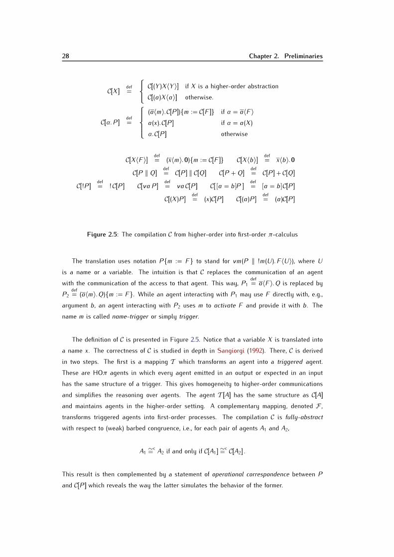
28 Chapter 2. Preliminaries
C[[X ]] def= C[[(Y )X〈Y 〉]] if X is a higher-order abstractionC[[(a)X〈a〉]] otherwise.
C[[α .P]] def=
(a〈m〉. C[[P]]){m := C[[F ]]} if α = a〈F〉a(x). C[[P]] if α = a(X )α . C[[P]] otherwiseC[[X〈F〉]] def= (x〈m〉. 0){m := C[[F ]]} C[[X〈b〉]] def= x〈b〉. 0C[[P ‖ Q]] def= C[[P]] ‖ C[[Q]] C[[P +Q]] def= C[[P]] + C[[Q]]C[[!P]] def= ! C[[P]] C[[νaP]] def= νa C[[P]] C[[ [a = b]P ]] def= [a = b] C[[P]]C[[(X )P]] def= (x)C[[P]] C[[(a)P]] def= (a)C[[P]]
Figure 2.5: The compilation C from higher-order into first-order π-calculusThe translation uses notation P{m := F} to stand for νm(P ‖ !m(U).F〈U〉), where Uis a name or a variable. The intuition is that C replaces the communication of an agentwith the communication of the access to that agent. This way, P1 def= a〈F〉.Q is replaced byP2 def= (a〈m〉.Q){m := F}. While an agent interacting with P1 may use F directly with, e.g.,argument b, an agent interacting with P2 uses m to activate F and provide it with b. Thename m is called name-trigger or simply trigger.The definition of C is presented in Figure 2.5. Notice that a variable X is translated intoa name x. The correctness of C is studied in depth in Sangiorgi (1992). There, C is derivedin two steps. The first is a mapping T which transforms an agent into a triggered agent.These are HOπ agents in which every agent emitted in an output or expected in an inputhas the same structure of a trigger. This gives homogeneity to higher-order communicationsand simplifies the reasoning over agents. The agent T [[A]] has the same structure as C[[A]]and maintains agents in the higher-order setting. A complementary mapping, denoted F ,transforms triggered agents into first-order processes. The compilation C is fully-abstractwith respect to (weak) barbed congruence, i.e., for each pair of agents A1 and A2,
A1 ∼=c A2 if and only if C[[A1]] ∼=c C[[A2]] .This result is then complemented by a statement of operational correspondence between Pand C[[P]] which reveals the way the latter simulates the behavior of the former.
2.2. Higher-Order Process Calculi 29
2.2.3 Other Higher-Order Languages
We review a number higher-order languages with concurrency, following the way they ap-peared in theoretical computer science:• As a way of studying the foundations of programming languages integrating functionaland concurrent paradigms. This is represented by variants of the λ-calculus enrichedwith forms of parallelism (see, e.g., (Boudol, 1989; Nielson, 1989)).• As a way of studying forms of code mobility and mobile agents. This is represented byprocess calculi with process-passing (see, e.g., (Thomsen, 1990; Sangiorgi, 1992; Schmittand Stefani, 2004; Hildebrandt et al., 2004)).In what follows we give an overview of both research strands, with an emphasis on theefforts concerning process calculi.
2.2.3.1 Functional Languages with Concurrency
A number of works advocated that a formal model for concurrent, communicating processesshould contain the λ-calculus as a simple sub-calculus.Boudol (1989) proposes the γ-calculus, a strict extension of lambda calculus with CCS-like communication. The γ-calculus is a direct generalization of the λ-calculus, in that aβ-reduction is formally defined to be a particular instance of the communication rule (and notsomething that is representable by a series of communications, for instance). The calculusis parametrized on a set of ports, and the parallel composition operator of CCS is splittedin two constructs: interleaving and cooperation, which represent concurrency and communi-cation, respectively. The cooperation operator is not associative, so λ-calculus application isrepresented by cooperation and output constructs. This way the desired (tight) relationshipbetween communication and application is achieved. Interestingly, in the γ-calculus the co-operation operator is “dynamic” in that reduction behind prefixes are allowed; much like asactive outputs in certain modern process calculi.In a similar spirit, Nielson (1989) proposes an extension of the typed λ-calculus withprocess communication. Here the role of types is indeed prominent, as they are meant torecord the communication possibilities of processes, while retaining the usual informationabout functions and tuples that is provided by the typed λ-calculus. Here “communicationpossibilities” refers essentially to the channels over which communication can occur and thetypes of the entities that can be communicated over these. The type system then results fromgeneralizing the notion of sort as defined in CCS; it guarantees that, given some expressione with type t, everything e evaluates to will also have type t, provided that e reads values ofpermissible types.

30 Chapter 2. Preliminaries
The FACILE language framework (Giacalone et al., 1989; Prasad et al., 1990) is an inte-gration of functional and concurrent programming. Unlike other proposals, which enrich oneof the programming styles with features of the other, FACILE intends to be symmetric in thata full functional language is integrated with a full concurrent language. In FACILE concurrentprocesses communicate through synchronous message passing; processes manipulate data infunctional style. While the operational definition of FACILE first given in (Giacalone et al.,1989) consisted of a translation into a concurrent functional abstract machine, in (Prasad et al.,1990) the semantic foundations of the framework are given in terms of a notion of programbehavior that combines the observable behavior of processes and the evaluation of expres-sions. Program equivalence is based on a form of contexts called windows, which are meantto index families of bisimulation relations. Roughly speaking, two expressions are equivalentif they reduce to equivalent values while producing equivalent behavior. The higher-ordernature of the language is reflected in the observational equivalence by developing the notionof equivalent actions to be based on the idea of equivalent values. This is like higher-orderbisimilarity defined in CHOCS.Finally, CML is a concurrent extension of Standard ML (Reppy, 1991, 1992) in which syn-chronous operations are treated as first-class values. Synchronous operations are representedin the set of values by events; the language provides combinators to construct complex eventsfrom event values. This way a wide range of synchronization abstractions can be constructed,which in turn allows to support different concurrency idioms.2.2.3.2 Process Calculi with Higher-Order Features
Here we review a number of concurrent languages which rely on a process calculi basis inorder to implement higher-order features.CHOCS and Plain CHOCS. Thomsen (1995, 1990) introduces and develops the basic theoryof CHOCS, an extension of CCS with process passing. Probably the most distinctive featureof CHOCS is the treatment of the restriction operator as a dynamic binder. This simplifiessignificantly several aspects of the theory, such as the definition of an algebraic theory anddenotational semantics. Similarly as in (Boudol, 1989), the behavioral equivalence definedfor CHOCS (higher-order bisimilarity) considers the bisimilarity of the values of the actions,rather than their equality. Higher-order bisimilarity is shown to be a congruence, and analgebraic theory for it is also developed. Main ideas of the type system developed by Nielson(1989) are adapted to CHOCS so as to define a notion of sorts. As for the observationalequivalence, internal actions are abstracted in the delayed style: an arbitrary number ofinternal actions are only allowed before a visible one. Using this definition, and similarly asin CCS, the observational equivalence is proven to be a congruence for sum-free processes.

2.2. Higher-Order Process Calculi 31
Finally, an extension of the Hennessy-Milner logic is proposed for characterizing higher-orderbisimilarity. The higher-order nature of the calculus is captured by enriching modalities with(i) formulas representing the processes sent or received, and (ii) the state after the transition.The expressiveness of the calculus is demonstrated by exhibiting encodings of the lambdacalculus (with several evaluation strategies) into CHOCS, as well as an interpretation of asimple imperative programming language into CHOCS.Inspired in the π-calculus, Plain CHOCS (Thomsen, 1993, 1990) results from consideringthe restriction operator in CHOCS as a static binder. The transition system for Plain CHOCSand the bisimilarity developed upon it follow closely those defined for the lazy λ-calculus(Abramsky, 1989). The relationship between Plain CHOCS and the π-calculus is exploredby means of encodings in the two directions. The encoding of Plain CHOCS into the π-calculus follows the strategy in Milner et al. (1992): the communication of a process in PlainCHOCS is represented in the π-calculus as the communication of a link to a trigger constructthat provides copies of the communicated process. This encoding is defined for the fragmentof Plain CHOCS without renaming. An alternative encoding that considers renaming byadmitting a set of names as parameter is also proposed. The encoding of the π-calculus intoPlain CHOCS is more involved: the communication of a name in the π-calculus is representedby the communication of a Plain CHOCS process that contains the (input, output) capabilitiesof a name. This process, so-called wire, is meant to be “plugged” into the context of agiven receiver by renaming operations that allow to “localize” the capabilities of the name.The encoding is then formalized as a two-level translation. In the first step, all free namesand input-bound names are translated into process variables. Names bound by restriction aresimply translated as names in Plain CHOCS. In the second step of the translation, the processvariables corresponding to free names in the π-calculus process are translated into names inPlain CHOCS.Bloom (1994) proposes a meta-theory for higher-order process calculi that generalizesCHOCS by considering constructs for broadcasting communication and interruption of processexecution. Computation is of two kinds: process algebraic and functional so the meta-theorysubsumes the name passing capabilities of the π-calculus and reduction as in the λ-calculus.The metatheory is typed; types of channels recognize input and output capabilities. The be-havioral equivalence investigated is a generalization of higher-order bisimulation as proposedby Boudol (1989) and Thomsen (1990), and is shown to be a congruence.
The Blue Calculus. The Blue calculus (Boudol, 1998) provides an integration of the λ-calculus with the π-calculus with the objective of obtaining a direct model for higher-orderconcurrency with the same expressive power of the π-calculus while offering a more convenientprogramming notation. The Blue calculus is endowed with a type system that encompasses

32 Chapter 2. Preliminaries
both Curry’s type inference for the λ-calculus and Milner’s sorting type system for the π-calculus. In a nutshell, the computational model of Blue is built around of a name-passingλ-calculus in which asynchronous messages might call for resources (or services) available inthe form of linear and “inexhaustible” declarations. Because of the unified rationale of Blue,programs in the λ-calculus and processes in the π-calculus have both a Blue interpretation;this way, the Blue calculus is useful to formalize a number of intuitions on the relationshipbetween the λ-calculus and the π-calculus as well as encodings of evaluation strategies ofthe former into the latter.The M-calculus. Schmitt and Stefani (2003, 2002) propose the M-calculus, a higher-orderdistributed calculus that provides the notion of hierarchical, programmable locality as a wayof representing those distributed systems in which localities can be of different kinds andexhibit different kinds of behaviors (e.g. with respect to access control or to failures). This isin sharp contrast with other calculi for distributed programming (such as the Ambient Calculus(Cardelli and Gordon, 2000)) in which localities are homogeneous, i.e. they are all of the samekind and have the same pre-defined behavior. This kind of distributed localities with explicit,programmable behavior are called cells; in combination with higher-order communication anddynamic binding features they allow to give a unified view of process migration and communi-cation. The design of the M-calculus retains features from the Blue Calculus (Boudol, 1998)and the Join calculus (Fournet et al., 1996); the M-calculus features a functional character inmessages (as in Blue), message patterns within definitions, and named cells so as to form atree-like hierarchy (as in Join). As a novelty, the M-calculus introduces a passivation operator,which can “freeze” running processes, and a type system for guaranteeing the unicity of namesof active cells are also introduced.The Kell calculus. The Kell calculus (Schmitt and Stefani, 2004) arises as a generalizationof the M-calculus, defined as a family of calculi intended to serve as a basis for component-based distributed programming. Built around a π-calculus core, the main features of the Kellcalculus are hierarchical, programmable localities and local actions. While the former areinherited from the M-calculus and allow to express different semantics for containment andmovement, the latter embody a principle under which atomic actions should occur within alocality, or at the boundary between a locality and its enclosing environment. Also as in theM-calculus, in Kell the execution of a process within a locality can be controlled through itspassivation. The Kell calculus can be instantiated by means of input pattern languages, i.e. thelanguage allowed in input constructs; this is most useful in defining a generic behavioral theoryfor the calculus. As a matter of fact, under sufficient conditions on substitution properties ofsuch pattern languages, a co-inductive characterization of contextual equivalence is providedin terms of a form of higher-order bisimulation termed strong context bisimulation.
2.2. Higher-Order Process Calculi 33
Homer. Homer (Hildebrandt et al., 2004) is a higher-order calculus for mobile embeddedresources. Its main features are active code mobility, explicit nested locations, and localnames. Given a resource (i.e. a process) inside a location, active process mobility refersto the fact that the resource might be taken (or pulled) by a suitable complementary prefix.This kind of movement sometimes referred to as objective mobility is a feature Homershares with the M-calculus and Kell. Crucially, and similarly as Boudol’s γ-calculus reviewedabove, the resource has the capability of performing internal computations inside locations,that is, the resource can evolve on its own before being moved. This is in sharp contrastto usual process passing and substitution. Location addresses are defined by nested names;interactions between resources at arbitrarily nested resources are allowed. These nestedlocations come with an involved treatment of local names, scope extension and extrusion. InHomer, barbed congruence is shown to be characterized by a labeled transition bisimulationcongruence.HOPLA. HOPLA (Nygaard and Winskel, 2002) is a higher-order language for non-deter-ministic processes that arises from a proposal for domain theory for concurrency; that is, froma denotational/categorical approach for giving meaning to concurrent computation. Roughlyspeaking, HOPLA is an extension of the typed λ-calculus in which a process is typed witha collection of its possible computation paths. The notion of prefix-sum type is introducedfor this purpose. The denotation of a process then relies on set-based operations on pathsand their extensions. HOPLA has a developed operational semantics and behavioral theory;sensible equivalences have been defined for it, including ordinary bisimilarity, applicativebisimilarity, and higher-order bisimilarity. An advantage of the domain-theoretical approachfor concurrency is that it is general by definition, and naturally leads to metalanguagesfor process description. This is evidenced in HOPLA, which can encode directly languagessuch as CCS, CCS with process passing, and mobile ambients. An extension of HOPLA thatincorporates name generation has been introduced in (Winskel and Zappa Nardelli, 2004).KLAIM. KLAIM (De Nicola et al., 1998) is a process description language: as such, itfalls between a programming language and a process calculi (see (De Nicola, 2006) for ashort survey on this distinction). In its process calculus dimension, processes and data can bemoved from one computing environment to another. KLAIM builds on the Linda tuple spacemodel, and can be seen as an asynchronous higher-order process calculus whose basic actionsare the original Linda primitives enriched with explicit information about the location of thenodes where processes and tuples are allocated. The behavioral theory for sub-languages ofKLAIM focuses on barbed congruence and may testing; it has been studied by Boreale et al.(1999).

34 Chapter 2. Preliminaries
Other proposals. In addition to the above mentioned calculi, other proposals of calculi forhigher-order concurrency can be found in the literature. For the sake of conciseness, we onlymention them without expanding in their details. Radestock and Eisenbach (1996) put forwarda higher-order process calculus for coordination in environments with distributed components.Ostrovsky et al. (2002) propose a higher-order process calculus with broadcasting communi-cation, and study its semantic theory in depth. Meredith and Radestock (2005b,a) proposea reflective higher-order process calculus in which names as in the π-calculus are obtainingby quoting processes. Hennessy et al. (2005) have proposed sophisticated type systems withdependent and existential types for a distributed version of the π-calculus with higher-ordercommunication of parametrized code. Mostrous and Yoshida (2007, 2009) have studied cal-culi for structured communication with higher-order communication and type disciplines forthem. Higher-order process calculi oriented towards security issues have been put forwardby Maffeis et al. (2008), who propose a higher-order spi-calculus (Abadi and Gordon, 1999)for code-carrying authorization, and by Sato and Sumii (2009), who define a higher-ordercalculus with cryptographic-like operations over terms such as decomposition. They rely inenvironmental bisimilarities to be reviewed later on for developing the behavioral theoryof their calculus.2.2.4 Behavioral Theory
Here we review some works that have addressed the behavioral theory for higher-order lan-guages. We concentrate on works for higher-order process calculi.Sangiorgi (1994) studies equivalences for versions of the λ-calculus possibly involving par-allelism. The objective is to find the finest behavioral equivalence on terms (i.e. the one thatdiscriminates the most). The starting point is Abramsky’s applicative bisimilarity for the lazyλ-calculus (Abramsky, 1989). Two approaches are followed. In the first one, the equivalenceinduced by the encoding of the lazy λ-calculus into the π-calculus (so-called lambda obser-vational equivalence) is studied. Such an equivalence is shown to be a congruence (using adirect proof, i.e. without using the encoding into pi), and fully-abstract with respect to Levy-Longo trees, the tree-like model for lazy λ-calculus terms. The second approach considersextensions of the pure λ-calculus. A rule format for well-formed operators is proposed for thatpurpose; intuitively, the rule format generates operators whose behavior only depends on theirsemantics, and not on their syntax. The most discriminating congruence is obtained when allwell-formed operators are admitted; such a congruence (so called rich applicative congruence)is shown to coincide with lambda observational equivalence. Non determinism is shown to bethe essential component for obtaining maximal discrimination.The definition of a satisfactory notion of bisimilarity is a hard problem for a higher-orderprocess language. In ordinary bisimilarity, as e.g. in CCS, two processes are bisimilar if any

2.2. Higher-Order Process Calculi 35
action by one of them can be matched by an equal action from the other in such a way thatthe resulting derivatives are again bisimilar. The two matching actions must be syntacticallyidentical. This condition is unacceptable in higher-order concurrency; for instance it breaksvital algebraic laws such as the commutativity of parallel composition. The approach takenby Thomsen (1990), following earlier ideas by Astesiano et al. (1988) and Boudol (1989), isto require bisimilarity rather than identity of the processes emitted in a higher-order outputaction. This weakening is natural for higher-order calculi and the bisimulation checks involvedare simple. Sangiorgi (1992) then argued that this form of bisimulation, called higher-orderbisimilarity, is in general troublesome or over-discriminating as a behavioral equivalence,and basic properties, such as congruence, may be very hard to establish. He then proposedcontext bisimilarity (1996a), a form of bisimilarity that avoids the separation between objectpart and continuation of an output action by explicitly taking into account the context in whichthe emitted agent is supposed to go. Context bisimilarity yields more satisfactory processequalities, and coincides with contextual equivalence (i.e., barbed congruence). However, ithas the drawback of a universal quantifications over contexts, which can make it hard, inpractice, to check equivalences.Normal bisimilarity (Sangiorgi, 1992; Jeffrey and Rathke, 2005; Cao, 2006) is a simplifica-tion of context bisimilarity without universal quantifications in the output clause. The inputclause is simpler too: normal bisimilarity can indeed be viewed as a form of open bisimilarity(Sangiorgi, 1996c), where the formal parameter of an input is not substituted in the inputclause, and free variables of terms are observable during the bisimulation game. However,the definition of the bisimilarity may depend on the operators in the calculus, and the cor-respondence with context bisimilarity may be hard to prove. The characterization of contextbisimilarity using normal bisimilarity in (Sangiorgi, 1996a) exploits triggered bisimilarity, anintermediate characterization of bisimilarity defined over triggered processes, i.e. a set ofprocesses in which every communication takes place by the exchange of a trigger. Sangiorgi(1996a) obtains this characterization for the weak case; however, the proof technique based ongoing through triggered agents does not carry over to the strong case, as it adds extra internalactions. Recently, Cao (2006) showed that strong/weak context bisimulation and strong/weaknormal bisimulation coincide in higher-order π-calculus. To do so, he goes through indexedbisimilarity, an equivalence defined over a variant of the calculus in which every prefix isindexed. Cao then uses indices to distinguish “internal” tau actions (those originating insidea component) from those “external” ones (those taking place among different components).The first which are essentially the kind of actions added by the encoding into triggeredprocesses are neglected in the indexed versions of the bisimulation games. Apart from set-tling the issue of the coincidence between normal and context bisimilarities in the strong case,the work in (Cao, 2006) provides a uniform setting for proving the coincidence of bisimilarities:

36 Chapter 2. Preliminaries
in the index-based proof technique the coincidence for the weak case results as a particularinstance.A drawback of the characterization of context bisimilarity with normal bisimilarity in (San-giorgi, 1996a) is that it is restricted to languages with finite types. Jeffrey and Rathke (2005)extends such a characterization to a language with recursive types. Their approach is basedon an enriched labeled transition system in which special operators representing referencesto triggers are included in the labels. As a result, a direct proof of soundness is possible,i.e., bisimilarity based on this enriched labeled transition system implies context bisimilarity.Completeness also holds; for the proof the original approach based on triggers is necessary.In addition to the definition of a suitable notion of bisimilarity, a related hard problem isthe proof that the bisimilarity is a congruence. In fact, for higher-order languages the “term-copying” feature inherited from the λ-calculus can make it hard to prove that bisimilarity is acongruence. A classical method for proving congruence of higher-order bisimulations is that ofHowe (1996). Originally introduced for (lazy) functional programming languages, this methodwas first adapted to higher-order process calculi by Baldamus (1998) and Thomsen (1989,1993) who used it for (variants of) CHOCS and Plain CHOCS. More recently, it has beenused by Ferreira et al. (1998) –for a concurrent version of ML– and by Hildebrandt et al.(2004; 2005), to show that late and input early bisimilarities are congruences in untyped andtyped versions of Homer.Recently, as a means of alleviating some of the problems Howe’s method entails when usedfor concurrent languages (most notably, its lack of flexibility), Sangiorgi et al. (2007) proposedenvironmental bisimulations, a method for higher-order languages that aims at make proofsof congruence easier and compatible with the so-called up-to techniques (Sangiorgi, 1998).Roughly, an environmental bisimulation makes a clear distinction between the terms testedin the bisimulation clauses and the environment, that is, an observer’s current knowledge. Assuch, for instance, in the output clause of the environmental bisimulation for HOπ, the emittedprocesses become part of the environment; the extruded names also receive special treatmentinside the clause. This is a more robust technique than previous approaches; it has beenapplied to both functional languages (pure λ-calculus and λ-calculus with information hiding)and to concurrent ones (Higher-Order π-calculus).Two very recent works develop further the theory of environmental bisimulations. Sato andSumii (2009) adapt and extend it in the setting of a higher-order, applied π-calculus featuringcryptographic operations such as encryption and decryption. Koutavas and Hennessy (2009)propose a first-order behavioral theory for higher-order processes based on the combinationof the principles of environmental bisimulations and the improvements to normal bisimilarityproposed by Jeffrey and Rathke (2005). At the heart of the proposed theory is a novel treatmentof name extrusions, which is formalized as an LTS in which configurations not only contain

2.3. Expressiveness of Concurrent Languages 37
the current knowledge of the environment and a process, but also information on the namesextruded by the process. As a consequence, the labels of such an LTS have a very simplestructure. The weak bisimilarity derived from this LTS is shown to be a congruence, fullyabstract with respect to contextual equivalence, and to have a logic characterization using avery simple Hennessy-Milner logic.Lenglet et al. (2009b, 2008, 2009a) have studied the behavioral theory of variants of higher-order π-calculi with restriction and/or passivation constructs. In (Lenglet et al., 2009b, 2008)they show that in a higher-order calculus with a passivation operator (such as Kell and Homer),the presence of a restriction operator disallows the characterization of barbed congruence bymeans of strong and normal bisimilarities. They use Howe’s method to prove congruenceof a weak higher-order bisimilarity for a calculus with passivation but without restriction.This result is improved in (Lenglet et al., 2009a) where barbed congruence is characterizedfor a higher-order process calculus with both passivation and restriction. To that end, theyexploit Howe’s method with the aid of so-called complementary semantics, which coincidewith contextual semantics and allow the use of Howe’s method to prove soundness of weakbisimilarities.The congruence of bisimilarity can also be approached by means of (syntactic) rule formats(see, e.g., (Mousavi et al., 2007), for a survey on formats and metatheory of structural opera-tional semantics). These are formats that induce congruence for any given notion of bisimilarityonce the rules of the operational semantics adhere to the formats. Bernstein (1998) proposesa rule format (promoted tyft/tyxy) for languages with higher-order features. The paper showsthat for any language defined in the format, strong bisimulation is a congruence. The ap-proach is applied to the lazy λ-calculus, the π-calculus, and CHOCS. In all cases, the studiedequivalence is bisimilarity; other behavioral equivalences, such as applicative bisimulation orhigher-order bisimulation, are not considered. Also, the format imposes a number of restric-tions on labels. In (Mousavi et al., 2005) both these shortcomings are studied. They buildon Bernstein’s work and propose a more general and relaxed rule format which induces con-gruence of (strong) higher-order bisimilarity. They use CHOCS to illustrate their rule format.The definition of suitable rule formats for other, more sensible, notions of bisimilarity (say,normal and context bisimilarity) is left in (Mousavi et al., 2005) as an open question.2.3 Expressiveness of Concurrent Languages
In this section we give a broad overview of the main approaches to the expressiveness ofconcurrent languages. We focus on the issues and techniques we shall use in this dissertation;the reader is referred to, e.g., (Parrow, 2008), for a recent survey on the area.We discuss on general issues in expressiveness in Section 2.3.1. Then, in Section 2.3.2,

38 Chapter 2. Preliminaries
we briefly review some of the notions of encoding that have been proposed in the literature.A classification of the main kinds of expressiveness results and the approaches to obtain themis presented in Section 2.3.3. Finally, we report on previous efforts on the expressiveness ofhigher-order concurrent languages (Section 2.3.4).Along the section, we shall follow a few notational conventions. We use L1,L2, . . . torange over languages; we use ≈ (possibly decorated) to denote a suitable behavioral equiva-lence. Also, −→ and =⇒ denote some (reduction) semantics and its reflexive, transitive closure,respectively.2.3.1 Generalities
An important criterion for assessing the significance of a paradigm is its expressiveness. Whilein other areas of computer science (most notably, automata theory), the notion of expressivenessis well-understood and settled, in concurrency theory there is yet no agreement on a formalcharacterization of the expressive power of a language, possibly with respect to that of someother language or model. While such a unified theory would be certainly desirable, the widevariety of existing models for concurrency (and consequently, of the expressiveness issuesinherent to them) strongly suggests that a single theory for language comparison embracingthem all does not exist.The crux of expressiveness studies is the notion of encoding, i.e., a function (or map)[[·]] from the terms of a source language into the terms of a target language that satisfiescertain correctness criteria. These criteria enforce both syntactic and semantic conditionson the nature of [[·]]. It is not difficult to see that the main source of difficulty in defining aunified theory for language comparison lies precisely in the exact definition of these criteria:depending on the purpose and on the given language(s), the set of applicable criteria mightvary and/or there might be criteria more adequate than others.From the point of view of their purpose, expressiveness studies can be broadly seen to beaimed at two kinds of results: encodability and non-encodability (or impossibility) results. Astheir name suggests, the former are concerned with the existence of an encoding, whereas thelatter address the opposite issue. These two kinds of questions are intimately related as, giventwo languages L1 and L2, in order to assert that L1 is more expressive than L2, one needs toprovide instances of both kinds of results: one should exhibit an encoding [[·]] : L2 → L1 and, atthe same time, one should provide a formal argument ensuring that an encoding [[·]] : L1 → L2does not exist. That is, it should be made clear that while L1 is able to express all thebehaviors of L2, there are some behaviors in L1 that L2 is unable to represent. It might thenappear clear that the correctness criteria for an encodability result should be different fromthose for an impossibility result. Indeed, for encodability results one would like to exhibit thebest encoding possible, i.e., one satisfying the most demanding correctness criteria possible; in
2.3. Expressiveness of Concurrent Languages 39
contrast, for impossibility results one would like to rely on the most general formal argument,i.e. one satisfying the least demanding correctness criteria possible. Not surprisingly, theproof techniques involved and the ingenuity required to obtain either result can be quitedifferent.Another broad classification of expressiveness studies takes into account whether or notthe expressive power of a given language is analyzed with respect to another language. Inother words, whether one is interested in absolute or in relative expressiveness.In studies of absolute expressiveness the interest is therefore in assessing the expressivepower that is intrinsic to the language and its associated semantics: as Parrow (2008) explains,this question entails determining exactly the transition systems as well as the operators onthem that are expressible in a given language. That is, the focus is on the expressivenessof the terms of the language, and on the kind of operators that are expressible in it. Thesequestions depend on suitable denotations of labeled transition systems, which explains the factthat expressiveness results of this kind have been reported only for basic process calculi, withrelatively simple labels (Parrow, 2008). A pioneering work in this direction is De Simone’sstudy of the expressive power of the MEIJE process algebra (de Simone, 1985). A seeminglywidespread approach to absolute expressiveness relies on some standard model of computationrather than on the semantic machinery of the language to assess the expressive power ofa language. A common yardstick here is Turing completeness, which is generally shown byexhibiting an encoding of some Turing-equivalent model into the given language. While thisapproach to absolute expressiveness sometimes referred to as computational expressiveness(see, e.g., Aranda (2009); Busi and Zandron (2009)) takes some external model as reference(and as such, it is not entirely “absolute”), the fact that such reference models are widelyknown and/or understood often constitutes a satisfactory measure of the intrinsic expressivepower of a language.In relative expressiveness one measures the expressive power of a given language L1by taking some other language L2 as a reference. This is particularly appealing when, forinstance, one wants to show that L1 and L2 have the same expressive power. In this case,the objective is to obtain two encodability results, one in each direction. Another commonsituation is when one wishes to determine the influence a particular operator or construct hason the expressiveness of a language L1. In this case, the reference language L2 is the fragmentof L1 without the operator(s) of interest. In this case, one aims at showing that L1 cannot beencoded into L2. If this can be done then the difference in the expressive power between thetwo languages has been singled out: it is in the operators that L1 has but that L2 lacks. Thisis sometimes referred to as a separation result, as the analyzed construct separates the worldwith it from the world without it (Yoshida, 2002).

40 Chapter 2. Preliminaries
2.3.2 The Notion of Encoding
We present a historical account of the evolution of definition of encoding, starting from propos-als within programming languages at large and concluding with the most relevant proposalsfor concurrent languages.2.3.2.1 Early Attempts to Expressiveness
It is instructive to examine the origin of the notions of expressiveness and expressive powerin the realm of programming languages at large. The earliest attempts towards a formalnotion of “expressive power” can be traced back to the late 1960s, when a proliferation ofprogramming languages was first noticed. Perhaps the most influential work of that periodis due to Landin (1966), who proposed a unified framework aimed at describing families ofprogramming languages from which particular languages can be derived by an appropriatechoice of primitives. Main concerns in Landin’s formal framework are conventions about user-defined names and functional relationships.Later on, in the early 1970s, the question of the expressive power was studied by repre-senting families of programs by means of program schemas, i.e., abstract representations ofprogramming features with uninterpreted constant and function symbols (see, e.g., (Chandraand Manna, 1976)). This line of research sometimes referred to as comparative schematol-ogy is mainly concerned about the expressiveness of single constructs.Felleisen (1991) developed a framework for expressiveness studies in the context of func-tional languages. His framework is suited for comparing a language and some extension of it;hence, it is suited for studies of relative expressiveness as introduced before. The frameworkdeparts from the idea of eliminable syntactic symbols as proposed in logic by Kleene andothers. More concretely, given two languages L1 and L2 such that L1 ⊆ L2, if the additionalsymbols/constructs of L2 are eliminable (with respect to L1) then L2 is said to be a definitionalextension of L1. Several notions and concepts that we shall encounter in “modern” studies ofexpressiveness of concurrent languages can be found already in Felleisen’s work. For instance,the crucial observation that the key to (programming) language comparison is a restriction onthe set of admissible translations between (programming) languages. This observation is rep-resented by structural (syntactic) and semantic conditions; while the former include notionssuch as compositionality of translations and homomorphism of a translation with respect tosome operator, the latter is represented by the preservation of terminating behavior, a naturalrequirement in a functional setting. In Felleisen’s view, the expressiveness of a programminglanguage is closely related to the programming discipline since, intuitively, programs writtenin the extension of some core language can be more readable than the programs written inthe core language.

2.3. Expressiveness of Concurrent Languages 41
Mitchell (1993) compares (functional) languages according to the ability of making sectionsof a program “abstract” by hiding some details of the internal functioning of the code. Hedefines so-called abstraction-preserving reductions, which are compositional translations thatpreserve observational equivalence. Perhaps the simplest reduction of this kind is the onetranslating program blocks into function declaration and calls. Proofs showing that moreinvolved reductions are abstraction-preserving might involve appealing to the operational anddenotational semantics of the languages in question. Riecke (1993) uses and extends thenotion of abstraction-preserving reductions in the study of the expressive power of differentevaluation strategies in the functional language PCF. He shows that call-by-value and lazyPCF are equally expressive, and that both are more expressive than call-by-name PCF.2.3.2.2 Encodings Among Concurrent Languages: The Early Days
Shapiro (1989) was the first to study expressiveness issues for concurrent languages. He pro-posed the notion of embedding as a way of comparing concurrent logic programming languages;considered languages are thus relatively similar and it is easy to focus on their differences. Anembedding is composed of a compiler and a viewer (or decoder). Given two languages L1 andL2, the compiler is a function c from programs of L1 into programs of L2, whereas the vieweris a function v from observables of L2 into observables of L1. Both c and v form an embeddingof L1 into L2 if the observables of every program P in L1 correspond to the observables ofthe program obtained by compiling P using c and viewing (or decoding) its behavior usingv . In order to define a hierarchy of concurrent logic programming languages, this notion ofembedding is tailored to the logic programming setting by requiring natural embeddings, i.e.,embeddings in which (a) the unification mechanism of one language is implemented in theunification mechanism of the other, and (b) logical variables of one language are mapped intological variables of the other. This proposal for language comparison was refined by Shapiro(1991) and by de Boer and Palamidessi (1990, 1994). We comment on both refinements next.Shapiro (1991) claims that no method similar to program schemas exists for comparison ofconcurrent languages. He then proposes a general framework for language comparison, whichrelies on the (non) existence of mappings that preserve the syntactic and semantic structureof the languages. Those mappings adhering to such preservation conditions are called em-beddings. The framework is expressed in categorical terms, and is general enough so asto work for any family of languages with syntactic operations and a semantic equivalence.Shapiro identifies three categories of embeddings that provide an incremental notion on thepreservation of the semantic structure of languages: sound embeddings, i.e. mappings thatpreserve observable distinctions; faithful embeddings, i.e. sound embeddings that preservethe semantic equivalence; fully-abstract embeddings, i.e. embeddings that are faithful withrespect to the congruence induced by the semantic equivalence. The work concentrates in
42 Chapter 2. Preliminaries
the formalization of separation results; a so-called separation schema arises from consideringparallel composition as the sole composition operation and by considering three properties:compositionality, i.e. the coincidence of the semantic equivalence with its induced congru-ence; interference-freedom, which disallows the parallel composition of a program with itself;hiding, i.e. the existence of programs that are semantically different from the trivial program,but whose composition is semantically equivalent to the trivial program. The framework forlanguage comparison is used to provide a number of separation results among several con-current languages and models, including Input/Output Automata, Actors, concurrent Prolog,and (variants of) CCS and CSP. In (Shapiro, 1992), the general framework is also shown to beuseful for formalizing positive (i.e. encodability) results.After observing that the notion of embedding introduced by Shapiro fell short for formalizingcertain separation results among concurrent constraint languages, de Boer and Palamidessi(1994) introduced the refined notion of modular embedding. A modular embedding is anembedding that satisfies the following three restrictions. First, since in the presence of non-determinism the domain of the observables of a language is a powerset, the decoder of theembedding is required to be defined elementwise on the elements on the set of observables.Second, the compiler is required to be compositional with respect to the parallel composi-tion and the non-deterministic choice operators. Third, the embedding must be terminationinvariant: a success (resp. deadlock or failure) in the target language must correspond to asuccess (resp. deadlock or failure) in the source language. The notion of modular encoding isthen used to derive separation results in the context of concurrent constraint languages withdifferent communication primitives in guarded-choice operators. The key idea to achieve sep-aration relies on a semantic argument: two variants are separated by showing that a certainclosure property is satisfied by the semantics of one variant but not by the semantics of theother. The notion of modular embedding was also used in (de Boer and Palamidessi, 1991)to show separation results for variants of CSP with different communication primitives in theguards. Indeed, it is shown that asynchronous CSP is strictly less expressive than CSP, thusconfirming results obtained by Bouge (1988), who exploited the capability each variant haveof expressing symmetric solutions to the leader election problem.2.3.2.3 Encodings Among Concurrent Languages: Towards “Modern” Criteria
The introduction of the π-calculus in the early 1990s gave a significant momentum to thestudy of expressiveness issues in process calculi. Indeed, the simplicity and flexibility of name-passing as embodied in the π-calculus triggered many works proposing variants or extensionsof it. Such works addressed a wide variety of concerns, including, e.g., polyadic communication(Milner, 1991), asynchronous communication (Boudol, 1992; Honda and Tokoro, 1991), higher-order communication (Thomsen, 1990; Sangiorgi, 1992), stochastic behavior (Priami, 1995),

2.3. Expressiveness of Concurrent Languages 43
structured communication (Honda et al., 1998), security protocols (Abadi and Gordon, 1999;Abadi and Fournet, 2001). While some of these variants were mainly only of theoreticalinterest, some others (e.g., (Priami, 1995; Abadi and Gordon, 1999)) were aimed at exploitingworking analogies between the behavior of mobile systems as in the π-calculus and that ofsystems in areas such as systems biology and security.In this context, expressiveness studies for the π-calculus were then indispensable to under-stand its fundamental properties, to identify the intrinsic sources of its expressive power, andto discern about the relationships between its many variants. As representative examples ofworks in these directions, we find studies on the properties of the translation of polyadic intomonadic π-calculus (Yoshida, 1996; Quaglia and Walker, 2005), on the relationship betweenpoint-to-point and broadcasting communication (Ene and Muntean, 1999), on the differentkinds of choice operators (Nestmann, 2000; Nestmann and Pierce, 2000) and, closely related,on mechanisms for synchronous and asynchronous communication (Palamidessi, 2003; Caccia-grano et al., 2007). Probably as a consequence of the different motivations for approachingexpressiveness, each of these works advocated its own definition of encoding, one in whichthe set of correctness criteria is defined in accordance to some specific working intuition ornecessity. In what follows we review some of those proposals and comment on their mainfeatures. For the sake of conciseness, we focus on a few, representative proposals namelythose by Sangiorgi (1992), Nestmann (1996), Palamidessi (2003), and Gorla (2008) in orderto give a broad overview to the area and to contrast certain aspects that we judge relevant.As part of his study on the relationship between first-order and higher-order π-calculus,Sangiorgi (1992) identifies three phases in determining that a given source language can berepresentable into some target language:1. Formal definition of the semantics of the two languages;2. Definition of the encoding from the source to the target language;3. Proof of correctness of the encoding with respect to the semantics given.Concerning the properties of (2), the only requirement is compositionality, that is, that thedefinition of the encoding of a term should only depend on the definition of its immediateconstituents. Given source and target languages Ls and Lt , an encoding [[·]] : Ls → Lt , andan n-adic construct op of Ls, compositionality can be expressed as follows:
[[op(P1, . . . , Pn)]] = Cop[[[P1]], . . . , [[Pn]]] (2.2)where Cop is a valid process context in Lt . As for correctness criteria, the main criteria adoptedis full-abstraction, i.e., two terms in the source language should be equivalent if and only iftheir translations are equivalent:
S1 ≈s S2 if and only [[S1]] ≈t [[S2]] . (2.3)

44 Chapter 2. Preliminaries
That is, full-abstraction enforces both preservation and reflection of the equivalence of sourceterms. Sangiorgi admits that full-abstraction represents a strong approach to representability.As we shall elaborate later, the purpose of Sangiorgi is to transfer reasoning techniquesfrom the first-order setting to the higher-order one. In this sense, requiring full abstractionturns out to be necessary, given that target terms should be usable in any context, and theindistinguishability of two source terms should imply that of their translations in order toswitch from one language to another. He also acknowledges that full-abstraction alone is notinformative enough with respect to the relationship between source and target terms. To thatend, he argues that full-abstraction should be complemented with some form of operationalcorrespondence relating a term and its translation.Based on his works on the encodability of choice operators into the (choice-free) π-calculus,Nestmann (1996) collects a number of desirable correctness criteria for encodings. As for full-abstraction, Nestmann comments that it might not applicable in those cases in which the sourcelanguage is not equipped with a notion of equivalence. Then, a suitable notion of operationalcorrespondence gains relevance. Operational correspondence is usually expressed as twocomplementary criteria. The first one, completeness, ensures the preservation of executionsteps, i.e., that the translation is able to simulate all the computations of the source term:S1 −→s S2 implies [[S1]] =⇒t [[S2]] . (2.4)
The second criteria, soundness, ensures the reflection of execution steps, i.e., that the behaviorof a term in the target language can be related to the behavior of its corresponding term inthe source language: [[S1]] =⇒t [[S2]] implies S1 =⇒s S2 . (2.5)However, soundness as in (2.5) is not satisfactory as it disregards the intermediate processesthe translation of a source term might need to go through in order to simulate its behavior. Arefinement that considers such intermediate steps is the following:
if [[S]] −→t [[T ]] then there is S −→s S′ such that [[T ]] ≈t [[S′]] . (2.6)A further refinement to soundness is the one that takes into account the administrative stepsthat an encoding might have to perform before simulating a step of the source term:
if [[S]] =⇒t [[T ]] then there is S =⇒s S′ such that [[T ]] =⇒t [[S′]] . (2.7)In addition to full-abstraction and operational correspondence, Nestmann (1996) considerstwo further correctness criteria effectiveness/efficiency and preservation/reflection of deadlocksand divergence. Let us elaborate only the latter criterion. Nestmann regards as interestingto consider both the reflection and preservation of deadlocks. The former is quite natural:the translation of a term should not deadlock if the given source term does not deadlock.

2.3. Expressiveness of Concurrent Languages 45
Preservation of deadlocks is also reasonable as long as potential administrative steps in thetarget side that might precede deadlock are taken into account. As for divergence, Nestmanndistinguishes between the kind of translation performed by compilers and that performed byencodings. Indeed, while a compiler is not expect to add divergent behavior, Nestmann findsan encoding that adds divergence perfectly acceptable. To put this position into context,it is worth noticing that the issue of divergence is central to the work in (Nestmann andPierce, 2000) where a trade-off between atomicity of committing a choice and divergence isdiscovered. In fact, Nestmann and Pierce (2000) propose two encodings of the π-calculuswith input-guarded choice into the choice-free fragment: one encoding is atomic with respectto choice but introduces divergence; the other encoding is divergence-free but replaces theatomic commitment of choice with gradual commitment. Therefore, there could be scenarios inwhich correct encodings that add divergence might still be worth having.A well-known definition of encoding is the one proposed by Palamidessi (2003) as part ofa comparison of the expressive power of synchronous and asynchronous communication in theπ-calculus. In short, she showed that there is no encoding of the synchronous π-calculus withmixed-choice into the asynchronous π-calculus without choice. This separation result holdsunder a notion of encoding in which syntactic criteria are captured by the notion of uniformity,which is given by the following two conditions:1. homomorphism with respect to parallel composition, i.e., [[P ‖ Q]] = [[P]] ‖ [[Q]];2. preservation of renaming, i.e. for any permutation of names σ in the domain of the targetlanguage, there exists a permutation θ in the domain of the target language such that,for all name i, σ (i) = θ(i) and [[σ (P)]] = θ([[P]]).Palamidessi argues that uniformity is tailored for the representations of distributed sys-tems, in which issues such as connectivity and coordination should be taken into account byany notion of encoding. This is particularly evident in requiring homomorphism with respectto parallel composition rather than generic compositionality as in (2.2) above. This can beconsidered as a strong syntactic criterion. However, as Palamidessi claims, in the context ofdistributed systems homomorphism with respect to parallel composition finds justification asit is essential to ensure that the encoding preserves the degree of distribution of the system,i.e. the encoding of a distributed system does not add coordinating processes (or sites).Furthermore, in Palamidessi’s expressiveness results, encodings are required to be seman-tically reasonable. Quoting Palamidessi (2003), encodings are required to preserve
a semantics which distinguishes two processes P and Q whenever there exists a(finite or infinite) computation of P in which the intended observables (some visibleactions) are different from the observables in any (maximal) computation of Q.

46 Chapter 2. Preliminaries
It is worth noticing that this is quite a liberal way of capturing requirements such as oper-ational correspondence and the reflection/preservation of deadlocks and divergence, discussedabove. Nestmann (2000) has studied the results in (Palamidessi, 2003) by taking correct-ness criteria more precise than “preservation of a reasonable semantics”. Indeed, he showsthat while the π-calculus with mixed-choice can be translated into into the asynchronous π-calculus, a trade-off between divergence and the exact notion of compositionality arises: thereare encodings that are uniform but that introduce divergence, whereas encodings that do notintroduce divergence only respect generic compositionality.Recent works have questioned the role of full-abstraction as a correctness criteria in en-codings of concurrent languages (see Beauxis et al. (2008) for an insightful discussion). Theirmotivation is that when one is interested in relative expressiveness rather than in, for in-stance, the transference of reasoning tools from one language to another full-abstractionis of little significance, as it is too focused on the actual equivalences considered. This isprecisely the motivation for a unified approach to correctness criteria in encodings recentlyproposed by Gorla (2008).Gorla’s proposal defines a kind of meta-theory for relative expressiveness, based on a setof encodability criteria formulated in abstract terms. As in (Felleisen, 1991), the criteria aredivided into structural (i.e., syntactic) and semantic. The former include a form of composition-ality as in (2.2) but where the context is parametrized by the set of free names of the sourceterms, and a condition on the independence from the actual names used in source terms thatgeneralizes condition (2) in the definition of uniform encoding given by Palamidessi. Semanticcriteria include a form of operational correspondence that is defined up to the “garbage terms”that an encoding might produce; divergence reflection, that is, that the encoding does not adddivergence; and success sensitiveness, i.e., a criteria that requires that based on some notion of“success computation” ensures that a successful source term is mapped into a successful targetterm. Sensible notions of success include observables such as barbs (Milner and Sangiorgi,1992) or the outcomes from tests as in behavioral equivalences/preorders based on testing (DeNicola and Hennessy, 1984). A significant advantage of the proposal in (Gorla, 2008) is that itcan be exploited by diverse concurrent languages (with different behavioral equivalences) and,to a certain extent, it can be used to reason abstractly about encodings and their properties.In order to illustrate its relevance, the proposal has been instantiated so as to obtain resultspreviously proposed in the literature (Gorla, 2006), and to offer more straightforward proofsfor other results.To conclude, these different proposals for the definition of encoding and its associatedcorrectness criteria only reinforce the idea that a unified notion of encoding is unlikely toexist. In fact, we have seen how the definitions vary depending on the final purpose of theexpressiveness study. Hence, a particular definition of encoding should not be judged solely
2.3. Expressiveness of Concurrent Languages 47
on the basis of its differences with respect to other notions of encoding, which will most likelybe aimed at different purposes. A current debate concerns the role of full-abstraction asadvocated by, e.g., Sangiorgi (1992). In our view, the crucial insight here is to understand that(i) the transference of reasoning techniques from one language to another and (ii) the study ofissues of relative expressiveness are essentially two different goals that expressiveness resultscan aim at. As such, one cannot expect correctness criteria aimed at (i) to make sense insettings in which the interest is in (ii), and viceversa.2.3.3 Main Approaches to Expressiveness
Having reviewed some representative definitions of encoding, here we propose a very broadclassification of approaches for obtaining expressiveness results. Our classification does notintend to be exhaustive or conclusive; it provides us with a way of presenting certain usedtechniques and to emphasize on their differences.2.3.3.1 Encodability of Computational Models
This is a rather widespread approach to studies of absolute expressiveness. The objective isto to demonstrate the (full) computational expressiveness of a language or model by means ofthe encodability of a Turing complete model. Notice that, under certain conditions, such anencoding is enough to demonstrate that most relevant decision problems are undecidable.Examples of Turing complete models used in expressiveness studies are Random AccessMachines (RAMs) (Shepherdson and Sturgis, 1963), Minsky machines (Minsky, 1967), andTuring machines. Roughly speaking, both RAMs and Minsky machines are models composedof registers (or counters) that hold natural numbers, a set of labeled instructions, and a programcounter indicating the instruction currently in execution. The main difference between the twois that while a RAM considers a finite set of registers, a Minsky machine requires only twoof them to ensure Turing completeness.One of the first works that have used this approach is (Busi et al., 2000) in which RAMsare encoded into variants of the coordination language Linda. In turn, such work has servedas inspiration for a number of works addressing similar concerns (see, e.g., (Busi and Zavat-taro, 2000, 2004; Busi et al., 2009; Maffeis and Phillips, 2005)). The use of complete Turingmachines (i.e. with a ribbon or tape, a transition relation, initial and accepting states) hasbeen reported by Hirschkoff et al. (2002) in their study of the expressiveness of the Ambientlogic. Similarly, Cardelli and Gordon (2000) have reported an encoding of Turing machinesin the Ambient calculus. In addition to Turing complete formalisms, models of computabilitystrictly less expressive than Turing machines have been considered for expressiveness pur-poses. Christensen (1993) shows that the class of languages generated by Basic ParallelProcesses (BPP, a fragment of CCS without communication nor restriction) is contained in the

48 Chapter 2. Preliminaries
class of context-sensitive languages. In the realm of (process) rewrite systems, efforts towardsa general Chomsky-like hierarchy of process languages have been made by Moller (1996) andby Mayr (2000). More recently, Aranda et al. (2007) study fragments of CCS with replicationare studied with respect to context-sensitive, context-free, and regular languages.The fact that several works have appealed to encodings of Turing complete models hasraised the question as to what criteria such encodings should satisfy. That is, the issue ofthe notion of encoding that is crucial to studies of relative expressiveness arises in issues ofabsolute expressiveness as well. In this case, the criteria are oriented towards determining howfaithful such encodings are with respect to the behavior of a Turing machine. In fact, notionsof Turing completeness that are “weaker” than the classical one have been put forward forexplaining the computational expressiveness of certain process calculi. Maffeis and Phillips(2005) and Bravetti and Zavattaro (2009) have analyzed and defined precisely these weakernotions. Let us recall such criteria, as identified by Bravetti and Zavattaro (2009).Definition 2.10 (Turing completeness for process calculi, (Bravetti and Zavattaro, 2009)). Alanguage L is said to be Turing complete, if given a partial recursive function with a giveninput, there is a process (i.e., a term of the language) in L such that
1. If the function is defined for the given input, then every computation of the processterminates and make the corresponding output available;2. If the function is not defined for the given input, then every computation of the processdoes not terminate.There are process calculi in which Turing complete models can be encoded in such a waythat at least the terminating computations respect the computations of the considered model.Such calculi satisfy the following weaker criterion.
Definition 2.11 (Weak Turing completeness for process calculi, (Bravetti and Zavattaro, 2009)).A language L is said to be weakly Turing complete, if given a partial recursive function witha given input, there is a process (i.e., a term of the language) in L such that1. If the function is defined for the given input, then there exists at least one computationof the process that terminates and make the corresponding output available;2. If the function is not defined for the given input, then every computation of the processdoes not terminate.Notice that the difference between the two notions is then in the first item. Indeed, if thefunction is defined according to the first notion every computation of the corresponding processterminates; in the second notion, the corresponding process may have computations that donot terminate. While encodings used to show Turing completeness for process calculi as in

2.3. Expressiveness of Concurrent Languages 49
M-INC i : INC(rj ) m′j = mj + 1 m′1−j = m1−j(i, m0, m1) −→M (i+ 1, m′0, m′1)M-DEC i : DECJ(rj , k) mj 6= 0 m′j = mj − 1 m′1−j = m1−j(i, m0, m1) −→M (i+ 1, m′0, m′1)
M-JMP i : DECJ(rj , k) mj = 0(i, m0, m1) −→M (k,m0, m1)
Figure 2.6: Reduction of Minsky machinesDefinition 2.10 are sometimes called deterministic or faithful (see, e.g., (Busi et al., 2009)). Incontrast, encodings used to show weak Turing completeness for process calculi as in Definition2.11 are called non-deterministic or not faithful (see, e.g., (Aranda, 2009)).In this dissertation we will consider calculi that satisfy the criteria given by Definition2.10, as well as calculi that satisfy the criterion given by Definition 2.11. In all cases, weshall exploit encodings of such calculi into Minsky machines. We therefore find it convenientto introduce such a model here.Minsky machines A Minsky machine (Minsky, 1967) is a Turing complete model composed ofa set of sequential, labeled instructions, and two registers. Registers rj (j ∈ {0, 1}) can holdarbitrarily large natural numbers. Instructions (1 : I1), . . . , (n : In) can be of two kinds: INC(rj )adds 1 to register rj and proceeds to the next instruction; DECJ(rj , k) jumps to instruction k ifrj is zero, otherwise it decreases register rj by 1 and proceeds to the next instruction.A Minsky machine includes a program counter p indicating the label of the instructionbeing executed. In its initial state, the machine has both registers set to 0 and the programcounter p set to the first instruction. The Minsky machine stops whenever the program counteris set to a non-existent instruction, i.e. p > n.A configuration of a Minsky machine is a tuple (i, m0, m1); it consists of the current programcounter and the values of the registers. Formally, the reduction relation over configurationsof a Minsky machine, denoted −→M, is defined in Figure 2.6.2.3.3.2 Decision/Representative Problems
This is an approach to separation results. As argued by Zavattaro (2009), the idea is to dis-criminate the expressiveness of two variants of the same computational model by investigating

50 Chapter 2. Preliminaries
the decidability of some decision problem in the two different settings. This allows one toprove that a different interpretation for a given concurrent computational model, or a simpleextension of one concurrent computational model, strictly increases the expressive power.An example of this line of research is (Dufourd et al., 1998) in which separation results forPetri nets with Reset arcs are obtained from the (un)decidability of decision problems such asreachability, termination, coverability, and boundness. In process calculi, this approach hasbeen pioneered by the already cited work on the expressiveness of variants of Linda (Busiet al., 2000) where the decidability of termination is used to prove a separation result be-tween two semantics of the language. Such a decidability result is obtained by endowing thelanguage with a net semantics (in terms of contextual Place/Transition nets) and by defininga deadlock-preserving mapping into finite Place/Transition nets. Another significant applica-tion of such approach is (Busi et al., 2009), in which separation results for variants of CCSwith different constructs for infinite behavior are reported. In (Busi et al., 2009) the focus ison the (un)decidability of termination and convergence of processes. It is shown that whileboth properties are undecidable for the variant of CCS with recursion, termination is decid-able for the variant for replication. While undecidability results are obtained by exhibiting(termination-preserving) encodings of RAMs (as described above), decidability results are ob-tained by appealing to the theory of well-structured transition systems (Abdulla et al., 2000;Finkel, 1990; Finkel and Schnoebelen, 2001). In Chapter 5 we shall apply the approach toseparation in (Busi et al., 2009) in the context of a higher-order process calculus.A somewhat related approach to separation results is the one that distinguishes two modelsbased on their capability of solving some well-established problem. That is, a language L1is considered to be more expressive than L2 if the problem can be solved in L1 but not inL2. This is a natural approach to follow when the languages at hand are both known to beTuring complete and hence a separation result based on the decidability of some property (asdiscussed before) is not an option.Inspired in results by Bouge (1988) in the context of CSP, this approach was used byPalamidessi (2003) for showing the separation between the π calculus with mixed-choice andthe asynchronous π-calculus with separate choice. The separation is demonstrated by thefact that, under certain conditions, the leader election problem a problem of distributedconsensus in the realm of distributed computing can be solved in the former but not in thelatter. This approach has been rather successful for it has been applied to a number of verydiverse calculi (see, e.g., Bouge (1988); Ene and Muntean (1999); Palamidessi (2003); Vigliottiet al. (2007)). More recently, the approach based on leader election has been intensivelystudied by Vigliotti (2004) in the context of the Ambient calculus. An excellent reference tothis approach (and to separation results in general) is (Vigliotti et al., 2007).Furthermore, while the use of widely known problems is a sensible option for separation

2.3. Expressiveness of Concurrent Languages 51
results, new problems have been also proposed. This way, for instance, Carbone and Maffeis(2003) have introduced matching systems so as to define an expressiveness hierarchy of variantsof the π-calculus with polyadic synchronization. Also, Versari et al. (2009) have proposed thelast man standing problem in order to assess the expressive power of variants of CCS withglobal and local prorities.2.3.3.3 By Combinators
This is a less studied approach to the expressiveness of concurrent languages. It aims at theassessing the expressive power of a language by identifying its set of combinators, i.e., theelements of the language that are indispensable to represent the whole behavior realizable inthe language. This is similar to the notion of combinators in the λ-calculus (Barendregt, 1984).Hence, each the combinators of a language is said to be essential for in the absence of one ofthem it is not possible to express the whole language (possibly up to semantic equivalences).Studying the expressiveness of a language based on combinators then appears as a usefulmethod to analyze and categorize its behavior.The earliest attempt in this direction is by Parrow (1990), where the focus is on theexpressiveness of two forms of parallel composition (called disjoint parallelism and linking)in the context of a small process calculus with synchronization primitives. Parrow identifiesthree “units” which are responsible for generating all the finite-state behavior that can beexpressed in the language. He also establishes conditions under which operators for parallelcomposition in other algebras can be defined. Parrow (2000) himself took this idea furtherto the context of mobile processes. In fact, he showed that every process in the synchronousπ-calculus without sum and without matching can be mapped (up to weak bisimilarity) as athe parallel composition of a number of trios, i.e., prefixes with length at most three, possiblyreplicated. It is also shown that duos, i.e., prefixes of length at most two, are not sufficient toproduce the same result. A similar result is shown by Laneve and Victor (2003) for the Fusioncalculus.Based on the results in (Honda and Yoshida, 1994a,b), Yoshida (2002) shows the minimalityof five concurrent combinators that characterize the expressive power of the asynchronous π-calculus without sum. Such combinators correspond to small processes implementing outputof messages, duplication of messages, and generation of links. Each of the five combinatorsis shown to be indispensable to represent the whole behavior of the calculus. Similar ideaswere explored by Raja and Shyamasundar (1995a,b).2.3.3.4 Other approaches
In a slightly different approach to expressiveness issues, a number of works has appealed tothe generality of structural operational semantics, their associated rule formats and properties,
52 Chapter 2. Preliminaries
as a way of gaining insights on the expressive power of languages that fit certain rule formats.For the sake of conciseness, we do not expand on these, and refer the interested reader to,e.g., (de Simone, 1985; Vaandrager, 1992; Dsouza and Bloom, 1995).2.3.4 Expressiveness for Higher-Order Languages
We conclude this section by reviewing a number of proposals that address the expressivenessof higher-order languages.Significant studies of the expressiveness of the higher-order communication paradigm arereported in Sangiorgi’s PhD dissertation (Sangiorgi, 1992). In Section 2.2.2 we have given themain ideas underlying the compilation C from higher-order into first-order processes, whichis central to his representability result. In (Sangiorgi, 1992) the compilation C is used tostudy encodings of (variants of) the λ-calculus into the π-calculus. An encoding of the lazyλ-calculus into HOπ, denoted H, is proposed. The encoding H enjoys a tight operationalcorrespondence; in fact, it allows to determine that the lazy λ-calculus is a sub-calculus ofHOπ. Furthermore, it is shown that the composition of C withH corresponds with the encodingof the lazy λ-calculus into the π-calculus proposed by Milner (1992). Hence, the usefulnessof C is shown by providing an alternative way of deriving results and transferring reasoningtechniques between the lazy λ-calculus and the π-calculus. A similar approach is followedfor the call-by-value λ-calculus.Amadio (1993) obtains a finitely-branching bisimilarity for CHOCS by means of a reduc-tion into bisimulation for a variant of the π-calculus. In such a variant, processes are onlyallowed to exchange names of activation channels (i.e. the channels that trigger a copy of aprocess in the representation of higher-order communication with first-order one). The desiredfinitely-branching bisimilarity is obtained by relying on a labeled transition system in whichsynchronizations on activation channels are distinguished.Amadio (1994) investigates Core Facile, a λ-calculus with synchronization primitives, par-allel composition, and dynamic creation of names. It is intended to serve as an intermediatelanguage between theoretical formalisms (such as CHOCS and the π-calculus) and actualprogramming languages such as Facile and CML. A control operator is introduced to ma-nipulate evaluation contexts and to define a translation of synchronous communication intoasynchronous one. This translation is shown to be adequate, i.e. equivalence of the translatedterms implies equivalence of the original terms. By means of a Continuation-Passing Styletranslation into Core Facile, the control operator is shown to be redundant. A translation ofthe asynchronous Core Facile into the π-calculus is also presented; this translation is furtherstudied in (Amadio et al., 1995).The expressiveness of the π-calculus wrt higher-order π was first studied by Sangiorgi(1996b), who isolated hierarchies of fragments of first-order and higher-order calculi with
2.3. Expressiveness of Concurrent Languages 53
increasingly expressive power. For the former, he identifies a fragment of the π-calculus inwhich mobility is internal, i.e., where outputs are only on private names no free outputsare allowed. This hierarchy is denoted as πIn, where the n denotes the degree of mobilityallowed; e.g., πI1 does not allow mobility and corresponds to the core of CCS. The hierarchy inthe higher-order case follows a similar rationale, and is based on the strictly higher-order π-calculus, i.e., a higher-order calculus without name-passing features. Also in this hierarchy, theless expressive language (denoted HOπ1) corresponds to the core of CCS. Sangiorgi showsthat πIn and HOπn have the same expressiveness, by exhibiting fully-abstract encodings.Sangiorgi and Walker’s encoding of a variant of π-calculus into Higher-Order π-calculus2001 relies on the abstraction mechanism of the Higher-Order π-calculus (it needs ω-orderabstractions).Vivas et al (Vivas and Dam, 1998; Vivas and Yoshida, 2002; Vivas, 2001) study extensionsof the higher-order π-calculus for which the usual encoding of higher-order into first-order(Sangiorgi, 1992) does not work. This is the case of higher-order calculi involving locations,in which certain operations cannot be reduced to reference passing, such as e.g., retrievingsome piece of code in a certain location and executing it elsewhere. This issue is first studiedby Vivas and Dam (1998) who show that Sangiorgi’s encoding schema breaks if blocking aform of restriction based on dynamic scoping is added to the language. Their motivation forsuch a construct is the modeling of cryptographic protocols; they claim that usual restriction(based on static scoping) as found in the first- and higher-order π-calculus is not adequatefor certain security scenarios. They consider first- and higher-order calculi with mismatching,and show that in the first-order case blocking has the same expressive power as matchingand mismatching. A rather involved schema for compiling higher-order calculi with blockinginto first-order calculi is proposed; it consists in the communication the syntax tree of aprocess. Vivas and Yoshida (2002) propose an extension of a higher-order process languagewith a screening operator called filtering. The objective is to represent scenarios of codemobility in which resource access control involves both static and dynamic checkings. Thefiltering operator is intended to dynamically restrict the visibility of channels of a process:a filtered process can only perform actions present in its associated set of polarized channelnames (i.e. channel names with either output or input capabilities). Similarly as blocking in(Vivas and Dam, 1998), the filtering operator exploits dynamic binding to implement a form ofencapsulation that blocks external communication in the filtered channels. In this case, theusual restriction operator is claimed to be inadequate as it might allow for scope extrusion ofthe filtered channels. The higher-order language with filtering is studied with respect to thehigher-order language proposed by Yoshida and Hennessy (1999) (which is, essentially, a call-by-value λ-calculus augmented with π-calculus operators). This language is endowed with atype system that assigns interface types to processes, i.e. a type that limits the resources a

54 Chapter 2. Preliminaries
process might have access. An encoding of the latter into the former is proposed as a way ofunderstanding how dynamic checkings enforced by the filtering operator can mimic the staticchecking enforced by the interface types. The paper shows that the encoding behaves correctlyonly in the cases in which name extrusion is not involved.Bundgaard et al. (2006) investigate the expressive power of Homer by encoding the syn-chronous π-calculus. They succeed in showing that that higher-order process-passing togetherwith mobile resources in, possibly local, named locations are enough to represent π-calculusname-passing. In the Homer case, because of the mobile computing resources and the nestedlocations, name-passing is a derived notion instead of a primitive. Similarly as the encodingby Thomsen (1990), the encoding of the π-calculus into Homer is not fully-compositional:names are translated at the top-level, separately from the transition of processes.Bundgaard et al. (2009) study two approaches for obtaining finite-control fragments ofHomer in which barbed bisimilarity is decidable. The first approach is based on a typesystem that bounds the size of processes in terms of their syntactic components (e.g. numberof parallel components, location nesting). The second approach exploits results for the π-calculus and uses an encoding of the π-calculus into Homer to transport them in the form ofa suitable subcalculus.

Chapter 3
A Core Calculus for Higher-Order Concurrency
In this chapter we introduce HOCORE, the core of calculi for higher-order concurrency suchas CHOCS (Thomsen, 1989), Plain CHOCS (Thomsen, 1993), and Higher-Order π-calculus(Sangiorgi, 1992, 1996a,b).The syntax and the semantics of the calculus are given in Section 3.1. Then, Section3.2 discusses the expressiveness of the language. The main result is an encoding of Minskymachines into HOCORE, which allows to infer that the language is Turing complete. Section3.3 provides some concluding remarks.3.1 The Calculus
Syntax. We use a, b, c to range over names (also called channels), and x, y, z to range overvariables; the sets of names and variables are disjoint.Definition 3.1. The set of HOCORE processes is given by the following syntax:
P, Q ::= a〈P〉 output| a(x).P input prefix| x process variable| P ‖ Q parallel composition| 0 nilAn input a(x).P binds the free occurrences of x in P. We write fv(P) for the set of freevariables in P, and bv(P) for the bound variables. We identify processes up to a renaming ofbound variables. A process is closed if it does not have free variables. In a statement, a nameis fresh if it is not among the names of the objects (processes, actions, etc.) of the statement.We abbreviate a(x).P, with x 6∈ fv(P), as a.P, a〈0〉 as a, and P1 ‖ . . . ‖ Pk as ∏ki=1 Pi.Similarly, we write ∏n1 P as an abbreviation for the parallel composition of n copies of P.

56 Chapter 3. A Core Calculus for Higher-Order Concurrency
Further, P{Q/x} denotes the componentwise and simultaneous substitution of variables x withprocesses Q in P (we assume members of x are distinct).The size of a process is defined as follows.Definition 3.2. The size of a process P, written #(P), is inductively defined as:
#(0) = 0 #(P ‖ Q) = #(P) + #(Q) #(x) = 1#(a〈P〉) = 1 + #(P) #(a(x).P) = 1 + #(P)Semantics. Now we describe the LTS, which is defined on open processes. There are threeforms of transitions: τ transitions P τ−→ P ′; input transitions P a(x)−−→ P ′, meaning that Pcan receive at a a process that will replace x in the continuation P ′; and output transitionsP a〈P ′〉−−−→ P ′′ meaning that P emits P ′ at a, and in doing so it evolves to P ′′. We use α toindicate a generic label of a transition. The notions of free and bound variables extend tolabels as expected.
INP a(x).P a(x)−−→ P OUT a〈P〉 a〈P〉−−−→ 0
ACT1 P1 α−→ P ′1 bv(α) ∩ fv(P2) = ∅P1 ‖ P2 α−→ P ′1 ‖ P2TAU1 P1 a〈P〉−−−→ P ′1 P2 a(x)−−→ P ′2P1 ‖ P2 τ−→ P ′1 ‖ P ′2{P/x}(We have omitted ACT2 and TAU2, the symmetric counterparts of the last two rules.)
Definition 3.3. The structural congruence relation is the smallest congruence generated bythe following laws:P ‖ 0 ≡ P, P1 ‖ P2 ≡ P2 ‖ P1, P1 ‖ (P2 ‖ P3) ≡ (P1 ‖ P2) ‖ P3.Reductions P −→ P ′ are defined as P ≡ τ−→≡ P ′. We now state a few results which willbe important later.
Lemma 3.1. If P α−→ P ′ and P ≡ Q then there exists Q′ such that Q α−→ Q′ and P ′ ≡ Q′.Proof. By induction on the derivation of P ≡ Q, then by case analysis on P α−→ Q.Definition 3.4. A variable x is guarded in P ∈ HOCORE (or simply guarded, when P is clearfrom the context) if x only occurs free in an output or in subexpressions of P of the form π.P ′,where π is any prefix. A process P ∈ HOCORE is guarded (or has guarded variables) if all itsfree variables are guarded.
In particular, notice that if x is guarded in P then it does not appear in evaluation contexts(i.e. contexts which allow transitions in the hole position), and if x is not free in P then it isguarded in P. In the lemma below, we recall that an output action from an open process maycontain free variables, thus α{R/x} is the action obtained from α by applying the substitution{R/x}.
3.2. Expressiveness of HOCORE 57
Lemma 3.2. Suppose that P ∈ HOCORE and variables x are guarded in P. Then, for allR ∈ HOCORE we have:1. If P α−→ P ′, with variables in R disjoint from those in P, α and x, then P{R/x} α{R/x}−−−−→P ′{R/x};2. If P{R/x} α ′−→ M′, with variables in R disjoint from those in P, α ′ and x, then there isP ′ such that P α−→ P ′ and M′ = P ′{R/x}, α ′ = α{R/x}.
Proof. By induction on the transitions.Lemma 3.3. For all P ∈ HOCORE and x there is P ′ ∈ HOCORE with x guarded in P ′, andn ≥ 0 such that
1. P ≡ P ′ ‖∏n1 x2. P{R/x} ≡ P ′{R/x} ‖∏n1 R , for all R ∈ HOCORE.Proof. By induction on the structure of processes.3.2 Expressiveness of HOCORE
We first present encodings of a simple form of guarded choice and guarded replication. Thenwe use such encodings to encode Minsky machines.3.2.1 Guarded Choice
We extend the HOCORE syntax with a simple form of guarded choice to choose between differentbehaviors. Assume, for instance, that ai should trigger Pi, for i ∈ {1, 2}. We write this asa1.P1 + a2.P2, and we write the choice of the behavior Pi as ai. We then have, for each i,the reduction (a1.P1 + a2.P2) ‖ ai −→ Pi. We encode these new operators as follows.[[a1.P1 + a2.P2]]+ = a1〈[[P1]]+〉 ‖ a2〈[[P2]]+〉[[a1]]+ = a2(x2).a1(x1). x1[[a2]]+ = a1(x1).a2(x2). x2
The translation is an homomorphism on the other operators. This way, [[ai]]+ for i ∈ {1, 2} isa process that consumes both Pi’s and spawns the one chosen. This encoding is correct aslong as all guards used in the choices are different and there is at most one message at aguard, a1 or a2 in the previous example, enabled at any given time. The encoding introducesan extra communication for every guarded choice.With a slight abuse of notation, in what follows we shall use disjoint sums inside HOCOREprocesses without explicitely referring to the encoding [[·]]+.

58 Chapter 3. A Core Calculus for Higher-Order Concurrency
3.2.2 Input-guarded Replication
We follow the standard encoding of replication in higher-order process calculi, adapting it toinput-guarded replication so as to make sure that diverging behaviors are not introduced. Asthere is no restriction in HOCORE, the encoding is not compositional and replications cannotbe nested.Definition 3.5. Assume a fresh name c. The encoding of input-guarded replication is asfollows: [[!a(z).P]]i! = a(z). (c(x). (x ‖ c〈x〉 ‖ P)) ‖ c〈a(z). (c(x). (x ‖ c〈x〉 ‖ P))〉where P contains no replications (nested replications are forbidden), and [[·]]i! is an homomor-phism on the other process constructs in HOCORE.
It is worth noticing that after the input on a, a copy of P is only released after a synchro-nization on c. More precisely, we have the following correctness statement. We use Q 9 todenote that there is no Q′ such that Q −→ Q′, both in HOCORE and for Minsky Machines.Lemma 3.1 (Correctness of [[·]]i!). Let P be a HOCORE process with non-nested input-guardedreplications.
• If [[P]]i! −→ Q then ∃P ′ such that P −→ P ′ and either [[P ′]]i! = Q or Q −→ [[P ′]]i!.• If P −→ P ′ then either [[P]]i! −→ [[P ′]]i! or [[P]]i! −→−→ [[P ′]]i!.• [[P]]i! 9 iff P 9.
Proof. By induction on the transitions.With a slight abuse of notation, in what follows we shall use input-guarded replicationsinside HOCORE processes without explicitely referring to the encoding [[·]]i!.
3.2.3 Minsky machines
We present an encoding of Minsky machines (see Section 2.3.3) into HOCORE. The encodingshows that HOCORE is Turing complete and, as the encoding preserves termination, it alsoshows that termination in HOCORE is undecidable. The only form of non-determinism in theencoding is due to possible unfoldings of (the encoding of) recursive definitions after they havebeen used; otherwise, at any step, in the encoding any process has at most one reduction.We first show how to count and test for zero in HOCORE; then, we present the encoding ofa Minsky machine into HOCORE, denoted as [[·]]M (see Table 3.1).

3.2. Expressiveness of HOCORE 59
INSTRUCTIONS (i : Ii)[[(i : INC(rj ))]]M = !pi. (incj ‖ ack .pi+1)[[(i : DECJ(rj , k))]]M = !pi. (decj ‖ ack . (zj .pk + nj .pi+1)REGISTERS rj[[rj = 0]]M = (incj . rSj 〈(| 0 |)j〉 + decj . (r0j ‖ zj )) ‖ REGj[[rj = m]]M = (incj . rSj 〈(| m |)j〉 + decj . (| m− 1 |)j ) ‖ REGjwhere:REGj = !r0j . (ack ‖ incj . rSj 〈(| 0 |)j〉 + decj . (r0j ‖ zj )) ‖!rSj (Y ). (ack ‖ incj . rSj 〈rSj 〈Y 〉 ‖ nj〉 + decj .Y )
(| k |)j = r0j ‖ nj if k = 0rSj 〈(| k − 1 |)j〉 ‖ nj if k > 0.
Figure 3.1: Encoding of Minsky machines into HOCORECounting in HOCORE. The cornerstone of our encoding is the definition of counters that maybe tested for zero. Numbers are represented as nested higher-order processes: the encodingof a number k+1 in register j , denoted (| k+1 |)j , is the parallel composition of two processes:rSj 〈(| k |)j〉 (the successor of (| k |)j ) and a flag nj . The encoding of zero comprises such a flag,as well as the message r0j . As an example, (| 2 |)j is rSj 〈rSj 〈r0j ‖ nj〉 ‖ nj〉 ‖ nj .
Registers. Registers are counters that may be incremented and decremented. They consistof two parts: their current state and two mutually recursive processes used to generate anew state after an increment or decrement of the register. The state depends on whether thecurrent value of the register is zero or not, but in both cases it consists of a choice between anincrement and a decrement. In case of an increment, a message on rSj is sent containing thecurrent register value, for instance m. This message is then received by the recursive definitionof rSj that creates a new state with value m+ 1, ready for further increment or decrement. Incase of a decrement, the behavior depends on the current value, as specified in the reductionrelation in Table 2.6. If the current value is zero, then it stays at zero, recreating the statecorresponding to zero for further operations using the message on r0j , and it spawns a flagzj indicating that a decrement on a zero-valued register has occurred. If the current value mis strictly greater than zero, then the process (| m − 1 |)j is spawned. If m was equal to 1,this puts the state of the register to zero (using a message on r0j ). Otherwise, it keeps themessage in a non-zero state, with value m − 1, using a message on rSj . In both cases a flagnj is spawned to indicate that the register was not equal to zero before the decrement. Whenan increment or decrement has been processed, that is when the new current state has beencreated, an acknowledgment is sent to proceed with the execution of the next instruction.
60 Chapter 3. A Core Calculus for Higher-Order Concurrency
Instructions. The encoding of instructions goes hand in hand with the encoding of registers.Each instruction (i : Ii) is a replicated process guarded by pi, which represents the programcounter when p = i. Once pi is consumed, the instruction is active and an interaction witha register occurs. In case of an increment instruction, the corresponding choice is sent to therelevant register and, upon reception of the acknowledgment, the next instruction is spawned.In case of a decrement, the corresponding choice is sent to the register, then an acknowledg-ment is received followed by a choice depending on whether the register was zero, resultingin a jump to the specified instruction, or the spawning of the next instruction otherwise.The encoding of a configuration of a Minsky machine thus requires a finite number of freshnames (linear on n, the number of instructions).Definition 3.6. Let N be a Minsky machine with registers r0 = m0, r1 = m1 and instructions(1 : I1), . . . , (n : In). Suppose fresh, pairwise different names r0j , rSj , p1, . . . , pn, incj , decj , ack(for j ∈ {0, 1}). Given the encodings in Table 3.1, a configuration (i, m0, m1) of N is encodedas pi ‖ [[r0 = m0]]M ‖ [[r1 = m1]]M ‖ n∏
i=1 [[(i : Ii)]]M .Correctness of the Encoding. In HOCORE, we write −→∗ for the reflexive and transitiveclosure of −→, and P ⇑ if P has an infinite sequence of reductions. Similarly, in Minskymachines −→∗M is the reflexive and transitive closure of −→M, and N ⇑M means that N hasan infinite sequence of reductions.Lemma 3.2. Let N be a Minsky machine. We have:
1. N −→∗M N′ iff [[N]]M −→∗ [[N′]]M;2. if [[N]]M −→∗ P1 and [[N]]M −→∗ P2, then there exists N′ such that P1 −→∗ [[N′]]M andP2 −→∗ [[N′]]M;3. N ⇑M iff [[N]]M ⇑.The proof of Lemma 3.2 relies on two properties. The first one, given by Lemma 3.3, ensuresthat for every computation of the Minsky machine the encoding can perform a finite, non-emptysequence of reductions that correspond to the one made by the machine. Using Lemma 3.1,the second property (Lemma 3.4) ensures that if the process encoding a Minsky machine has areduction then (i) the machine also has a reduction, and (ii) the encoding has a finite sequenceof reductions that correspond to the result of the reduction of the Minsky machine.We now proceed with the proofs. In what follows we assume a Minsky machine N withinstructions (1 : I1), . . . , (n : In) and with registers r0 = m0 and r1 = m1. The encoding of aconfiguration (i, m0, m1) of N is denoted [[(i, m0, m1)N ]]M. We use −→j to stand for a sequenceof j reductions.

3.2. Expressiveness of HOCORE 61
Lemma 3.3. Let (i, m0, m1) be a configuration of a Minsky machine N.If (i, m0, m1) −→M (i′, m′0, m′1) then there exist a finite j and a process P such that[[(i, m0, m1)N ]]M −→j P and P = [[(i′, m′0, m′1)N ]]M.Proof. We proceed by case analysis on the instruction performed by the Minsky machine.Hence, we distinguish three cases corresponding to the behaviors associated to rules M-JMP,M-DEC, and M-INC.Case M-JMP We have a Minsky configuration (i, m0, m1) with m0 = 0 and (i : DECJ(r0, k)).By Definition 3.6, its encoding in HOCORE is as follows:
[[(i, m0, m1)N ]]M = pi ‖ [[r0 = 0]]M ‖ [[r1 = m1]]M ‖[[(i : DECJ(r0, k))]]M ‖ ∏l=1..n,l 6=i[[(l : Il)]]M
We begin by noting that the program counter pi is consumed by the encoding of the instructioni. The content of the instruction is thus exposed, and we then have[[(i, m0, m1)N ]]M −→ [[r0 = 0]]M ‖ dec0 ‖ ack . (z0.pk + n0.pi+1) ‖ S = P1
where S = [[r1 = m1]]M ‖ ∏nl=1[[(l : Il)]]M stands for the rest of the system. The only transitionpossible at this point is the behavior selection on dec0, which yields the following:P1 −→ r00 ‖ z0 ‖ REG0 ‖ ack . (z0.pk + n0.pi+1) ‖ S = P2
Now there is a synchronization between r00 and REG0 for reconstructing the registerP2 −→ z0 ‖ ack ‖ (inc0. rS0 〈(| 0 |)0〉 + dec0. (r00 ‖ z0)) ‖ REG0 ‖ack . (z0.pk + n0.pi+1) ‖ S = P3
Once the register has been re-created, register and instruction can now synchronize on ack:P3 −→ z0 ‖ (inc0. rS0 〈(| 0 |)0〉 + dec0. (r00 ‖ z0)) ‖ REG0 ‖z0.pk + n0.pi+1 ‖ S = P4
At this point, the only possible transition is the behavior selection on z0, which indicates thatthe content of r0 was indeed zero:P4 −→ (inc0. rS0 〈(| 0 |)0〉 + dec0. (r00 ‖ z0)) ‖ REG0 ‖ pk ‖ S = P5
Using the definitions of [[·]]M and S, and some reordering, we note that P5 can be equivalentlywritten as P5 = pk ‖ [[r0 = 0]]M ‖ [[r1 = m1]]M ‖ n∏l=1 [[(l : Il)]]M
which, in turn, corresponds to the encoding of [[(k, 0, m1)N ]]M, as desired.

62 Chapter 3. A Core Calculus for Higher-Order Concurrency
Case M-DEC We have a Minsky configuration (i, m0, m1) with m0 = c (for some c > 0) and(i : DECJ(r0, k)). By Definition 3.6, its encoding in HOCORE is as follows:[[(i, m0, m1)N ]]M = pi ‖ [[r0 = c]]M ‖ [[r1 = m1]]M ‖[[(i : DECJ(r0, k))]]M ‖ ∏
l=1..n,l 6=i[[(l : Il)]]MWe begin by noting that the program counter pi is consumed by the encoding of the instructioni. The content of the instruction is thus exposed, and we then have
[[(i, m0, m1)N ]]M −→ [[r0 = c]]M ‖ dec0 ‖ ack . (z0.pk + n0.pi+1) ‖ S = P1where S = [[r1 = m1]]M ‖ ∏nl=1[[(l : Il)]]M stands for the rest of the system. The only transitionpossible at this point is the behavior selection on dec0, which yields the following:
P1 −→ (| c − 1 |)0 ‖ REG0 ‖ ack . (z0.pk + n0.pi+1) ‖ S = P2It is worth recalling that (| c − 1 |)0 = rS0 〈(| c − 2 |)0〉 ‖ n0. Considering this, now there is asynchronization between rS0 and REG0 for decrementing the value of the register
P2 −→ n0 ‖ ack ‖ (inc0. (rS0 〈(| c − 1 |)0〉 ‖ n0) + dec0. (| c − 2 |)0) ‖ REG0 ‖ack . (z0.pk + n0.pi+1) ‖ S = P3Once the register has been re-created, register and instruction can now synchronize on ack:
P3 −→ n0 ‖ (inc0. (rS0 〈(| c − 1 |)0〉 ‖ n0) + dec0. (| c − 2 |)0) ‖ REG0 ‖z0.pk + n0.pi+1 ‖ S = P4At this point, the only possible transition is the behavior selection on n0, which indicates thatthe content of r0 was greater than zero:
P4 −→ (inc0. (rS0 〈(| c − 1 |)0〉 ‖ n0) + dec0. (| c − 2 |)0) ‖ REG0 ‖ pi+1 ‖ S = P5Using the definitions of [[·]]M and S, and some reordering, we note that P5 can be equivalentlywritten as P5 = pi+1 ‖ [[r0 = c − 1]]M ‖ [[r1 = m1]]M ‖ n∏
l=1 [[(l : Il)]]Mwhich, in turn, corresponds to the encoding of [[(i+ 1, c − 1, m1)N ]]M, as desired.Case M-INC We have a Minsky configuration (i, m0, m1) with (i : INC(r0)). Its encoding inHOCORE is as follows:
[[(i, m0, m1)N ]]M = pi ‖ [[r0 = m0]]M ‖ [[r1 = m1]]M ‖[[(i : INC(r0))]]M ‖ ∏l=1..n,l 6=i[[(l : Il)]]M

3.2. Expressiveness of HOCORE 63
We begin by noting that the program counter pi is consumed by the encoding of the instructioni: [[(i, m0, m1)N ]]M −→ [[r0 = m0]]M ‖ inc0 ‖ ack .pi+1 ‖ S = P1where S = [[r1 = m1]]M ‖ ∏nl=1[[(l : Il)]]M stands for the rest of the system. The only transitionpossible at this point is the behavior selection on inc0. After such a selection we haveP1 −→ rS0 〈(| m0 |)0〉 ‖ REG0 ‖ ack .pi+1 ‖ S = P2
Now there is a synchronization between rS0 and REG0 for incrementing the value of theregisterP2 −→ ack ‖ (inc0. (rS0 〈rS0 〈(| m0 |)0〉 ‖ n0〉) + dec0. ((| m0 |)0)) ‖ REG0 ‖ack .pi+1 ‖ S = P3
Once the register has been re-created, a synchronization on ack is possibleP3 −→ (inc0. (rS0 〈rS0 〈(| m0 |)0〉 ‖ n0〉) + dec0. ((| m0 |)0)) ‖ REG0 ‖pi+1 ‖ S = P4
Using the definition of (| · |)j we note that P4 actually corresponds toP4 = (inc0. (rS0 〈(| m0 + 1 |)0〉 + dec0. ((| m0 |)0)) ‖ REG0 ‖ pi+1 ‖ S
which in turn can be written asP4 = pi+1 ‖ [[r0 = m0 + 1]]M ‖ [[r1 = m1]]M ‖ n∏
l=1 [[(l : Il)]]Mwhich corresponds to the encoding of [[(i+ 1, m0 + 1, m1)N ]]M, as desired.Lemma 3.4. Let (i, m0, m1) be a configuration of a Minsky machine N.If [[(i, m0, m1)N ]]M −→ P1 then for every computation of P1 there exists a Pj such that Pj =[[(i′, m′0, m′1)N ]]M and (i, m0, m1) −→M (i′, m′0, m′1).Proof. Consider the reduction [[(i, m0, m1)N ]]M −→ P1. An analysis of the structure of process[[(i, m0, m1)N ]]M reveals that, in all cases, the only possibility for the first step correspondsto the consumption of the program counter pi. This implies that there exists an instructionlabeled with i, that can be executed from the configuration (i, m0, m1). We proceed by a caseanalysis on the possible instruction, considering also the fact that the register on which theinstruction acts can hold a value equal or greater than zero. In all cases, it can be shown thatcomputation evolves deterministically, until reaching a process in which a new program counter(that is, some pi′ ) appears. The program counter pi′ is inside a process that corresponds to[[(i′, m′0, m′1)N ]]M, where (i, m0, m1) −→M (i′, m′0, m′1). The analysis follows the same lines as theone reported for the proof of Lemma 3.3, and we omit it.

64 Chapter 3. A Core Calculus for Higher-Order Concurrency
Lemma 3.5. Let N be a Minsky machine. We have that N 9M if and only if [[N]]M 9.Proof. Straightforward from Lemmas 3.3 and 3.4.
The results above guarantee that HOCORE is Turing complete, and since the encodingpreserves termination, it entails the following corollary.Corollary 3.1. Termination in HOCORE is undecidable.3.3 Concluding Remarks
The encoding of Turing complete models (such as Minsky and Random Access Machines,RAMs) is a common proof technique for carrying out expressiveness studies. Our encodingof Minsky machines into HOCORE resembles in structure those in (Busi et al., 2003, 2009)where RAMs are used to investigate the expressive power of restriction and replication inname-passing calculi, and those in (Busi and Zavattaro, 2004), where the impact of restrictionand movement on the expressiveness of Ambient calculi is studied. The similarities can beexplained by the fact that all the encodings share the same guiding principle: representingcounting as the nesting of suitable components. Those components are restricted namesin CCS (Busi et al., 2009), recursive definitions in π-calculus (Busi et al., 2003), ambientsthemselves in Ambient calculus (Busi and Zavattaro, 2004), and higher-order messages in ourcase. Note that by combining our encoding with the one of higher-order π into π-calculus in(Sangiorgi and Walker, 2001), we obtain an encoding very similar to the one in (Busi et al.,2003). However, we do not know of other works using Turing complete models for provingexpressiveness results in the context of higher-order process calculi.

Chapter 4
Behavioral Theory of HOCORE
This chapter develops the behavioral theory of HOCORE. In Section 4.1 a notion of strongbisimilarity for HOCORE is studied; such a notion it is unique in that it coincides with othersensible behavioral equivalences in the higher-order setting. The most remarkable propertyof strong bisimilarity in HOCORE is that it is decidable. Section 4.2 analyzes the relationshipbetween strong bisimilarity and (asynchronous) barbed congruence. Section 4.3 introduces asound and complete axiomatization of strong bisimilarity. This axiomatization is then used toobtain an upper bound to the complexity of the bisimilarity problem. In Section 4.4 it is shownthat strong bisimilarity becoms undecidable if at least four static restriction are added to thecalculus. Section 4.5 briefly analyzes the impact of some extensions to the language on thedecidability results. Section 4.6 concludes.4.1 Bisimilarity in HOCORE
In this section we prove that the main forms of strong bisimilarity for higher-order processcalculi coincide in HOCORE, and that such a relation is decidable. As a key ingredient forour results, we introduce open Input/Output (IO) bisimulations in which the variable of inputprefixes is never instantiated and τ-transitions are not observed. To the best of our knowledge,HOCORE is the first calculus where IO bisimulation is discriminating enough to provide a usefulcharacterization of process behavior.We define different kinds of bisimulations by appropriate combinations of the clauses below.Definition 4.1 (HOCORE bisimulation clauses, open processes). A symmetric relation R onHOCORE processes is
1. a τ-bisimulation if P R Q and P τ−→ P ′ imply that there is Q′ such that Q τ−→ Q′ andP ′ R Q′;

66 Chapter 4. Behavioral Theory of HOCORE
2. a higher-order output bisimulation if P R Q and P a〈P ′′〉−−−→ P ′ imply that there are Q′, Q′′such that Q a〈Q′′〉−−−→ Q′ with P ′ R Q′ and P ′′ R Q′′;3. an output normal bisimulation if P R Q and P a〈P ′′〉−−−→ P ′ imply that there are Q′, Q′′such that Q a〈Q′′〉−−−→ Q′ with m.P ′′ ‖ P ′ R m.Q′′ ‖ Q′, where m is fresh.4. an open bisimulation if whenever P R Q:
• P a(x)−−→ P ′ implies that there is Q′ such that Q a(x)−−→ Q′ and P ′ R Q′,• P ≡ x ‖ P ′ implies that there is Q′ such that Q ≡ x ‖ Q′ and P ′ R Q′.Definition 4.2 (HOCORE bisimulation clauses, closed processes). A symmetric relation R onclosed HOCORE processes is
1. an output context bisimulation if P R Q and P a〈P ′′〉−−−→ P ′ imply that there are Q′, Q′′ suchthat Q a〈Q′′〉−−−→ Q′ and for all S with fv(S) ⊆ x, it holds that S{P ′′/x} ‖ P ′ R S{Q′′/x} ‖ Q′;2. an input normal bisimulation if P R Q and P a(x)−−→ P ′ imply that there is Q′ such thatQ a(x)−−→ Q′ and P ′{m〈0〉/x} R Q′{m〈0〉/x}, where m is fresh;3. closed if P R Q and P a(x)−−→ P ′ imply that there is Q′ such that Q a(x)−−→ Q′ and for allclosed R , it holds that P ′{R/x} R Q′{R/x}.A combination of the bisimulation clauses in Definitions 4.1 and 4.2 is complete if itincludes exactly one clause for input and output transitions (in contrast, it need not includea clause for τ-transitions).1 We will show that all complete combinations coincide. We onlygive a name to those combinations that represent known forms of bisimulation for higher-orderprocesses or that are needed in our proofs. In each case, as usual, a bisimilarity is the unionof all bisimulations, and is itself a bisimulation (the functions from relations to relations thatrepresent the bisimulation clauses in Definitions 4.1 and 4.2 are all monotonic).
Definition 4.3. Higher-order bisimilarity, written∼HO, is the largest relation on closed HOCOREprocesses that is a τ-bisimulation, a higher-order output bisimulation, and is closed.Context bisimilarity, written ∼CON, is the largest relation on closed HOCORE processes thatis a τ-bisimulation, an output context bisimulation, and is closed.Normal bisimilarity, written ∼NOR, is the largest relation on closed HOCORE processes thatis a τ-bisimulation, an output normal bisimulation, and an input normal bisimulation.IO bisimilarity, written ∼oIO, is the largest relation on HOCORE processes that is a higher-order output bisimulation and is open.Open normal bisimilarity, written ∼oNOR, is the largest relation on HOCORE processes thatis a τ-bisimulation, an output normal bisimulation, and is open.1The clauses of Definition 4.2 are however tailored to closed processes, therefore combining them with clause 4in Definition 4.1 has little interest.

4.1. Bisimilarity in HOCORE 67
Environmental bisimilarity (Sangiorgi et al., 2007), a recent proposal of bisimilarity forhigher-order calculi, in HOCORE roughly corresponds to (and indeed coincides with) the com-plete combination that is a τ-bisimulation, an output normal bisimulation, and is closed.Remark 4.1. The input clause of Definition 4.2(3) is in the late style. It is known (Sangiorgi,1992) that in calculi of pure higher-order concurrency early and late clauses are equivalent.Remark 4.2. In contrast with ordinary normal bisimulation (Sangiorgi, 1992; Jeffrey andRathke, 2005), our clause for output normal bisimulation does not use a replication in front ofthe introduced fresh name. Such a replication would be needed in extensions of the calculus(e.g., with recursion or restriction).
A bisimilarity on closed processes is extended to open processes as follows.Definition 4.4 (Extension of bisimilarities). Let R be a bisimilarity on closed HOCORE pro-cesses. The extension of R to open HOCORE processes is defined by
Ro = {(P,Q) : a(x1). · · · .a(xn).PRa(x1). · · · .a(xn).Q}where fv(P) ∪ fv(Q) = {x1, . . . , xn}, and a is fresh in P,Q.
The simplest complete form of bisimilarity is ∼oIO. Not only ∼oIO is the less demandingfor proofs; it also has a straightforward proof of congruence. This is significant becausecongruence is a notoriously hard problem in bisimilarities for higher-order calculi. Beforedescribing the proof of congruence for ∼oIO, we first define an auxiliary up-to technique thatwill be useful later.Definition 4.5. A symmetric relation R on HOCORE is an open IO bisimulation up-to ≡ ifP R Q implies:
1. if P a(x)−−→ P ′ then Q a(x)−−→ Q′ and P ′ ≡R≡ Q′;2. if P a〈P ′′〉−−−→ P ′ then Q a〈Q′′〉−−−→ Q′ with P ′ ≡R≡ Q′ and P ′′ ≡R≡ Q′′;3. if P ≡ x ‖ P ′ then Q ≡ x ‖ Q′ and P ′ ≡R≡ Q′.
Lemma 4.1. If R is an open IO bisimulation up-to ≡ and (P,Q) ∈ R then P ∼oIO Q.Proof. The proof proceeds by a standard diagram-chasing argument (as in, e.g., (Milner, 1989)):using Lemma 5.1 one shows that ≡R ≡ is a ∼oIO-bisimulation.
We now give the congruence result for ∼oIO.Lemma 4.2 (Congruence of ∼oIO). Let P1, P2 be open HOCORE processes. P1 ∼oIO P2 implies:
1. a(x).P1 ∼oIO a(x).P2

68 Chapter 4. Behavioral Theory of HOCORE
2. P1 ‖ R ∼oIO P2 ‖ R , for every R3. a〈P1〉 ∼oIO a〈P2〉
Proof. Items (1) and (3) are straightforward by showing the appropriate ∼oIO-bisimulations.We consider only (2). We show that, for every R , P1, and P2S = {(P1 ‖ R, P2 ‖ R) : P1 ∼oIO P2}
is a ∼oIO-bisimulation. We first suppose P1 ‖ R α−→ P ′; we need to find a matching actionfrom P2 ‖ R . We proceed by case analysis on the rule used to infer α . There are two cases.In the first one P1 α−→ P ′1 and P ′ = P ′1 ‖ R is inferred using rule ACT1 (by α-conversion wecan ensure that R respects the side condition of the rule). By definition of ∼oIO-bisimulation,P2 α−→ P ′2 with P ′1 ∼oIO P ′2. Using rule ACT1 we infer that also P2 ‖ R α−→ P ′2 ‖ R . We concludethat (P ′1 ‖ R,P ′2 ‖ R) ∈ S. The second case follows by an analogous argument and occurswhen R α−→ R ′ so that P ′ = P1 ‖ R ′ by rule ACT2.The last thing to consider is when P1 ‖ R ≡ x ‖ P ′; we need to show that P2 ‖ R ≡ x ‖ Q′and that (P ′, Q′) ∈ S. We distinguish two cases, depending on the shape of P ′. First, assumethat P ′ ≡ P ′1 ‖ R , that is, x is a subprocess of P1. Since P1 ∼oIO P2, then it must be thatP2 ≡ x ‖ P ′2 for some P ′2, with P ′1 ∼oIO P ′2. Taking Q′ ≡ P ′2 ‖ R we thus have (P ′, Q′) ∈ S.Second, assume x is a subprocess of R , and we have P ′ ≡ P1 ‖ R ′, we then take Q′ ≡ P2 ‖ R ′.Since S is defined over every R , then (P ′, Q′) ∈ S.Lemma 4.3 (∼oIO is preserved by substitutions). If P ∼oIO Q then for all x and R , alsoP{R/x} ∼oIO Q{R/x}.Proof. We show that, for processes P,Q in which x is guarded,
R = {(P{R/x} ‖ L, Q{R/x} ‖ L) : P ∼oIO Q}is a ∼oIO-bisimulation up-to ≡ (Definition 4.5). (This suffices, because of Lemma 4.1.) Considera pair (P{R/x} ‖ L, Q{R/x} ‖ L) ∈R. We shall concentrate on the possible moves from P{R/x},say P{R/x} α−→ P ′; transitions from L, if any, can be handled analogously. We proceed bycase analysis on the rule used to infer α .We only detail the case in which α is an input action a(x) inferred using rule INP; thecase in which α is an output is similar (there may be a substitution on the label). Since xis guarded in P, using Lemma 3.2(2), there is P1 such that P a(x)−−→ P1 and P ′ = P1{R/x}.By definition of ∼oIO-bisimulation, also Q a(x)−−→ Q1 with P1 ∼oIO Q1. Hence, by Lemma 3.2(1),Q{R/x} a(x)−−→ Q1{R/x}. It remains to show that P1{R/x} and Q1{R/x} can be rewritten into theform required in the bisimulation. Using Lemma 3.3(1), we have
P1 ≡ P ′1 ‖ n∏ x and Q1 ≡ Q′1 ‖ m∏ x
4.1. Bisimilarity in HOCORE 69
for P ′1, Q′1 in which x is guarded. As P1 ∼oIO Q1, it must be n = m and P ′1 ∼oIO Q′1. Finally,using Lemmas 3.3(2) and 4.2 we haveP1{R/x} ≡ P ′1{R/x} ‖ n∏R and Q1{R/x} ≡ Q′1{R/x} ‖ n∏R
which closes up the bisimulation up-to ≡.The most striking property of∼oIO is its decidability. In contrast with the other bisimilarities,in ∼oIO the size of processes always decreases during the bisimulation game. This is because∼oIO is an open relation and does not have a clause for τ transitions, hence process copyingnever occurs.
Lemma 4.4. Relation ∼oIO is decidable.Next we show that ∼oIO is also a τ bisimulation. This will allow us to prove that ∼oIO coin-cides with other bisimilarities, and to transfer to them its properties, in particular congruenceand decidability.
Lemma 4.5. Relation ∼oIO is a τ-bisimulation.Proof. Suppose (P,Q) ∈ ∼oIO and P τ−→ P ′; we have to find a matching transition Q τ−→ Q′.Action τ was inferred using either rule TAU1 or TAU2, so we have two cases. We consider onlythe first one as the second is analogous. If rule TAU1 was used, then we can decompose P’stransition into an output P a〈R〉−−−→ P1 followed by an input P1 a(x)−−→ P2, with P ′ = P2{R/x} (thatis, the structure of P is P ≡ a〈R〉 ‖ a(x).P2). By definition of ∼oIO, Q is capable of matchingthese two transitions, and the final derivative is a process Q2 with Q2 ∼oIO P2. Further, asHOCORE has no output prefixes (i.e., it is an asynchronous calculus) the two transitions from Qcan be combined into a τ-transition. Finally, since ∼oIO is preserved by substitutions (Lemma4.3), we can use rule TAU1 to derive a process Q′ = Q2{R/x} that matches the τ-transitionfrom P, with (P ′, Q′) ∈ ∼oIO.Corollary 4.1. ∼HO and ∼oIO coincide.Proof. The hard implication is the one right to left (∼oIO implies ∼HO). One shows that forclosed P,Q, ∼oIO is a∼HO-bisimulation. Suppose (P1, P2) ∈∼oIO and P1 α−→ Q1; we need to finda matching transition P2 α−→ Q2. We consider three cases, one for each form that α can take.Case α = a〈R〉 is immediate as both ∼HO and ∼oIO are higher-order output bisimulations. Asfor cases α = a(x) and α = τ, the desired transition can be easily obtained using Lemmas 4.3(∼oIO is preserved by substitutions) and 4.5 (∼oIO is a τ-bisimulation), respectively.
We thus infer that ∼HO is a congruence relation. A direct proof of this result (by exhibitingan appropriate bisimulation), in particular congruence for parallel composition, would have
70 Chapter 4. Behavioral Theory of HOCORE
been harder. Congruence of higher-order bisimilarity is usually proved by appealing to, andadapting, Howe’s method for the λ-calculus (Howe, 1996).We now move to the relationship between ∼HO, ∼oNOR, and ∼CON. We begin by establishinga few properties of normal bisimulation.Lemma 4.6. If m.P1 ‖ P ∼oNOR m.Q1 ‖ Q, for some fresh m, then we have P1 ∼oNOR Q1 andP ∼oNOR Q.Proof. We show that, for any fresh names m1, . . .,
S = ∞⋃j=1{(P, Q) : P ‖ ∏
k∈1..jmk .Pk ∼oNOR Q ‖ ∏k∈1..jmk .Qk}
S1= ∞⋃j=1{(P1, Q1) : P ‖ ∏
k∈1..jmk .Pk ∼oNOR Q ‖ ∏k∈1..jmk .Qk}
are ∼oNOR-bisimulations.We start with S. Suppose (P,Q) ∈S and that P α−→ P ′; we need to show a matchingaction from Q. We have different cases depending on the shape of α . We consider only thecase α = a〈P ′′〉, the others being simpler. By ACT1 we haveP ‖ ∏
k∈1..jmk .Pk a〈P ′′〉−−−→ P ′ ‖ ∏k∈1..jmk .Pk .
Since P ‖∏k∈1..j mk .Pk ∼oNOR Q ‖∏k∈1..j mk .Qk , there should exist a Q∗ such thatQ ‖ ∏
k∈1..jmk .Qk a〈Q′′〉−−−→ Q∗ ,with P ′ ‖ ∏k∈1..j mk .Pk ‖ m′′.P ′′ ∼oNOR Q∗ ‖ m′′.Q′′. As m1, . . . , mj are fresh, they do notoccur in P, thus a〈P ′′〉 does not mention them. For the same reason, there cannot be anycommunication between ∏k∈1..j mk .Qk and Q; so, we infer that the only possible transition is
Q ‖ ∏k∈1..jmk .Qk a〈Q′′〉−−−→ Q∗ = Q′ ‖ ∏
k∈1..jmk .Qk ,applying rule ACT1 toQ a〈Q′′〉−−−→ Q′. Since P ′ ‖∏k∈1..j mk .Pk ‖ m′′.P ′′ ∼oNOR Q′ ‖∏k∈1..j mk .Qk ‖m′′.Q′′, we have (P ′, Q′) ∈ S as needed.Before considering S1, we find it useful to detail a procedure for consuming ∼oNOR-bisimilarprocesses.Given a process P, let o(P) denote the number of output actions in P. Let m(P) =#(P) + o(P) be the measure that considers both the (lexical) size of P and the number ofoutput actions in it. Consider now two ∼oNOR-bisimilar processes P and Q. The procedureconsists in consuming one of them by performing its actions completely; the other process canmatch these actions (as it is ∼oNOR-bisimilar) and will be consumed as well. We will show that

4.1. Bisimilarity in HOCORE 71
m(P) decreases at each step of the bisimulation game; at the end, we will obtain processesPn and Qn with m(Pn) = m(Qn) = 0.To illustrate the procedure, suppose, w.l.o.g., process P has the following shape:P ≡ ∏
h∈1..t xh ‖∏i∈1..k ai(xi).Pi ‖
∏j∈1..lbj〈Pj〉where we have t top-level variables, k input actions, and l output actions. We use ai and bjfor channels in input and output actions, respectively. The first step is to remove top-levelvariables; this relies on the fact ∼oNOR is an open bisimilarity. One thus obtains processes P1and Q1 with only input and output actions, and both m(P1) < m(P) and m(Q1) < m(Q) hold.As a second step, the procedure exercises every output action in P1. By definition of ∼oNOR,Q1 should be able to match those actions. Call the resulting processes P2 and Q2. Recallthat when an output a〈Pj〉 is consumed in the bisimulation game, process mj .Pj is added inparallel. Thus since #(a〈P〉j ) = #(mj .Pj ) and the number of outputs decreases, measure mdecreases as well. More precisely, one has that
P2 ≡ ∏i∈1..k ai(xi).Pi ‖
∏j∈1..lmj .Pj
where mj stands for a fresh name. Then, one has to consider the k + l input actions in eachprocess; their consumption proceeds as expected. One obtains processes P3 and Q3 that arebisimilar, with strictly decreasing measures for both processes. The procedure concludes byiterating the above steps on P3 and Q3. In fact, we have shown that at each step measure mstrictly decreases; this guarantees that eventually one will reach processes Pn and Qn, withm(Pn) = m(Qn) = 0 as desired.With the above procedure showing S1 is a bisimulation is straightforward. Take the ∼oNOR-bisimilar processes P ‖ ∏k∈1..j mk .Pk and Q ‖ ∏k∈1..j mk .Qk . Using the procedure aboveover P and Q we obtain ∏k∈1..j mk .Pk ∼oNOR ∏k∈1..j mk .Qk . This is because fresh namesm1, . . . , mj do not occur in P and Q, and hence they do not intervene in P and Q’s consumption.Similarly, we can consume ∏k ′∈2..j mk ′ .Pk ′ (i.e. all the components excepting m1.P1) and thecorresponding ∏k ′∈2..j mk ′ .Qk ′ . We thus end up with m1.P1 ∼oNOR m1.Q1, and we observe thatthe only possible action on each side is the input on m1, which can be trivially matched bythe other. We then infer that (P1, Q1) ∈S1, as desired.Lemma 4.7. ∼HO implies ∼CON.Proof. We suppose (P,Q) ∈ ∼HO and P α−→ P ′; we need to show a matching action from Q.We proceed by case analysis on the form α can take. The only interesting case is when αis a higher-order output; the remaining clauses are the same in both relations. By definitionof ∼HO, if P a〈P ′′〉−−−→ P ′ then Q a〈Q′′〉−−−→ Q′, with both P ′′ ∼HO Q′′ and P ′ ∼HO Q′. We need toshow that, for every S such that fv(S) = {x}, S{P ′′/x} ‖ P ′ ∼HO S{Q′′/x} ‖ Q′; this follows

72 Chapter 4. Behavioral Theory of HOCORE
from P ′′ ∼HO Q′′ and P ′ ∼HO Q′ and the fact that ∼HO is both a congruence and preservedby substitutions.Lemma 4.8. ∼CON implies ∼NOR.Proof. Straightforward by showing an appropriate bisimulation. The result is immediate bynoticing that (i) both relations are τ-bisimulations, and that (ii) the input and output clausesof ∼NOR are instances of those of ∼CON. In the output case, by selecting a process S = m. x(with m fresh) one obtains the desired form for the clause. The input clause is similar, andfollows from the definition of closed bisimulation, which holds for every closed process R ; inparticular, it also holds for R = m〈0〉 (with m fresh) as required by the clause of ∼NOR.Lemma 4.9. ∼NOR implies ∼oNOR.Proof. We consider open processes, and as such, in what follows we consider the extension of∼NOR to open processes as in Definition 4.3, which we denote ∼?NOR. Notice that since ∼NORis an input normal bisimulation (Definition 4.2(2)), ∼?NOR can be equivalently defined as
P ∼?NOR Q iff P{m1〈0〉/x1, . . . ,mn〈0〉/xn} ∼NOR Q{m1〈0〉/x1, . . . ,mn〈0〉/xn}where {x1, . . . , xn} = fv(P) ∪ fv(Q) and m1, . . . , mn are fresh names. We will show that ∼?NORis an open normal bisimulation.We first suppose P ∼?NOR Q and P α−→ P ′; we need to find a matching transition Q α−→ Q′.We perform a case analysis on the shape α can take. In all cases, one uses the defini-tion of ∼?NOR to show that the desired transition actually takes place. Next, we only de-tail the case in which α = a(x), so we suppose P a(x)−−→ P ′. Now, if P a(x)−−→ P ′ then alsoP{m1〈0〉/x1, . . . ,mn〈0〉/xn} must be capable of performing such an action, so that
P{m1〈0〉/x1, . . . ,mn〈0〉/xn} a(x)−−→ P ′{m1〈0〉/x1, . . . ,mn〈0〉/xn}exists. In turn, by definition of ∼NOR, such an action guarantees that there exists a Q′ thatmatches that input action, i.e.
Q{m1〈0〉/x1, . . . ,mn〈0〉/xn} a(x)−−→ Q′{m1〈0〉/x1, . . . ,mn〈0〉/xn};with P ′{m1〈0〉/x1, . . . ,mn〈0〉/xn}{m〈0〉/x} ∼NOR Q′{m1〈0〉/x1, . . . ,mn〈0〉/xn}{m〈0〉/x}.Again, by using the definition the ∼?NOR on the above facts, it is easy to see that there is aQ′ such that Q a(x)−−→ Q′ and P ′ ∼?NOR Q′, and we are done.The last thing to consider are those variables in evaluation context in the open processes.This is straightforward by noting that by definition of ∼?NOR, all such variables have beenclosed with a trigger. So, suppose P ∼?NOR Q and
P{m1〈0〉/x1, . . . ,mn〈0〉/x} ≡ m1〈0〉 ‖ P ′{m1〈0〉/x1, . . . ,mn〈0〉/xn}
4.1. Bisimilarity in HOCORE 73
where m1 is fresh. We need to show that Q has a similar structure, i.e. that Q ≡ x ‖ Q′, withP ′ ∼?NOR Q′. P can perform an output action on m1, thus evolving to P ′{m1〈0〉/x1, . . . ,mn〈0〉/xn}.By definition of ∼?NOR, Q can match this action, and evolves to some process Q∗, with m′. 0 ‖P ′{m1〈0〉/x1, . . . ,mn〈0〉/xn} ∼?NOR m′. 0 ‖ Q∗, where m′ is a fresh name (obtained from thedefinition of ∼?NOR for output actions). The input on m′ can be trivially consumed on bothsides, and one has P ′{m1〈0〉/x1, . . . ,mn〈0〉/xn} ∼?NOR Q∗. At this point, since m1 is a freshname, we know that Q involves a variable in evaluation context. Furthermore, since there is acorrespondence between P ′ and Q∗, they should involve substitutions in the very same freshnames. More precisely, we have that there should be a Q′ such thatQ ≡ m1〈0〉 ‖ Q′{m1〈0〉/x1, . . . ,mn〈0〉/xn} = m1〈0〉 ‖ Q∗
as desired.Lemma 4.10. ∼oNOR implies ∼oIO.Proof. The only difference between the bisimilarities is their output clause: they are bothopen bisimulations. We analyze directly the case for output action. Suppose P ∼oNOR Q andP a〈P ′′〉−−−→ P ′; we need to show a matching action from Q. By definition of ∼oNOR, if P a〈P ′′〉−−−→ P ′then also Q a〈Q′′〉−−−→ Q′, with m.P ′′ ‖ P ′ ∼oNOR m.Q′′ ‖ Q′. Using this and Lemma 4.6 weconclude that P ′′ ∼oNOR Q′′ and P ′ ∼oNOR Q′.Lemma 4.11. In HOCORE, relations ∼HO, ∼oNOR and ∼CON coincide.Proof. This is an immediate consequence of previous results. In fact, we have proved (on openprocesses) the following implications:
1. ∼oIO implies ∼HO (Corollary 4.1).2. ∼HO implies ∼CON (Lemma 4.7);3. ∼CON implies ∼NOR (Lemma 4.8);4. ∼NOR implies ∼oNOR (Lemma 4.9);5. ∼oNOR implies ∼oIO (Lemma 4.10).
We then extend the result to all complete combinations of the HOCORE bisimulation clauses(Definitions 4.1 and 4.2).Theorem 4.1. All complete combinations of the HOCORE bisimulation clauses coincide, andare decidable.

74 Chapter 4. Behavioral Theory of HOCORE
Proof. In Lemma 4.11 we have proved that the least demanding combination (∼oIO) coincideswith the most demanding ones (∼HO and ∼CON). Decidability then follows from Lemma 4.4.We find this “collapsing” of bisimilarities in HOCORE significant; the only similar result weare aware of is by Cao (2006), who showed that strong context bisimulation and strong normalbisimulation coincide in higher-order π-calculus.
4.2 Barbed Congruence and Asynchronous Equivalences
We now show that the labeled bisimilarities of Section 4.1 coincide with barbed congruence,the form of contextual equivalence used in concurrency to justify bisimulation-like relations.Below we use reduction-closed barbed congruence (Honda and Yoshida, 1995; Sangiorgi andWalker, 2001), as this makes some technical details simpler; however the results also hold forordinary barbed congruence (Milner and Sangiorgi, 1992). It is worth recalling that the maindifference between reduction-closed and ordinary barbed congruence is quantification overcontexts (see (2) in Definition 4.6 below). More importantly, we consider the asynchronousversion of barbed congruence, where barbs are only produced by output messages; in syn-chronous barbed congruence inputs may also contribute. We use the asynchronous version fortwo reasons. First, asynchronous barbed congruence is a weaker relation, which makes theresults stronger (they imply the corresponding results for the synchronous relation). Second,asynchronous barbed congruence is more natural in HOCORE because it is an asynchronouscalculus it has no output prefix.Note also that the labeled bisimilarities of Section 4.1 have been defined in the syn-chronous style. In an asynchronous labeled bisimilarity (see, e.g., (Amadio et al., 1998)) theinput clause is weakened so as to allow, in certain conditions, an input action to be matchedalso by a τ-action. For instance, input normal bisimulation (Definition 4.2(2)) would become:• if P a(x)−−→ P ′ then, for some fresh name m,
1. either Q a(x)−−→ Q′ and P ′{m〈0〉/x} R Q′{m〈0〉/x};2. or Q τ−→ Q′ and P ′{m〈0〉/x} R Q′ ‖ a〈m〈0〉〉.
We now define asynchronous barbed congruence. We write P ↓a (resp. P ↓a) if P canperform an output (resp. input) transition at a.Definition 4.6. Asynchronous barbed congruence, ', is the largest symmetric relation onclosed processes that is
1. a τ-bisimulation (Definition 4.1(1));2. context-closed (i.e., P ' Q implies C [P] ' C [Q], for all closed contexts C [·]);
4.2. Barbed Congruence and Asynchronous Equivalences 75
3. barb preserving (i.e., if P ' Q and P ↓a, then also Q ↓a).In synchronous barbed congruence, input barbs P ↓a are also observable.
Lemma 4.12. Asynchronous barbed congruence coincides with normal bisimilarity.Proof. We first show that ∼NOR implies ', and then its converse, which is harder. Therelation ∼NOR satisfies the conditions in Definition 4.6 as follows. First, both relations areτ-bisimulations so condition (1) above trivially holds. Second, the context-closure conditionfollows from the fact that ∼NOR is a congruence. Finally, the barb-preserving condition is seento hold by definition of ∼NOR: having P ∼NOR Q implies that an output action of P on a hasto be matched by an output action of Q on a; hence, we have that if P ↓a, then also Q ↓a.Now the converse. We show that relation ' satisfies the three conditions for ∼NOR inDefinition 4.3. Suppose P ' Q and P α−→ P ′; we have to show a matching transition Q α−→ Q′.We proceed by a case analysis on the form α can take.Case α = τ Since by definition ' is a τ-bisimulation, then there is a Q′ such that Q τ−→ Q′and P ′ ' Q′ and we are done.Case α = a〈P ′′〉 We have P a〈P ′′〉−−−→ P ′: it can be shown that ' is an output normal bisimu-lation by showing a suitable context. Let Cao [·] be the context
Cao [·] = [·] ‖ a(x). (m. x ‖ n ‖ n. 0)where m,n are fresh names. We then have Cao [P] τ−→ P1 with P1 ↓n. Indeed, we haveP1 ≡ P ′ ‖ m.P ′′ ‖ n ‖ n. 0. By definition of ', we have also Cao [Q] τ−→ Q1 and necessarily,Q1 ↓n. Since n is a fresh name, we infer that Q also has an output on a, such that Q a〈Q′′〉−−−→ Q′and hence Q1 ≡ Q′ ‖ m.Q′′ ‖ n ‖ n. 0. Note that (P1, Q1) is in '. They can consume theactions on n; since it is a fresh name, only the corresponding τ action of Q1 can match it. Asa result, both processes evolve to processes P ′ ‖ m.P ′′ and Q′ ‖ m.Q′′ that are still in '. Wethen conclude that ' is an output normal bisimulation.Case α = a(x) We have P a(x)−−→ P ′. Again, to show that ' is an input normal bisimulation, wedefine a suitable context. Here, the asynchronous nature of HOCORE (more precisely, the lackof output prefixes, which prevents the control of output actions by modifying their continuation)and the input clause for ∼NOR it induces (reported above) result in a more involved definitionof these contexts. Notice that simply defining a context with an output action on a so as toforce synchronization with the input action does not work here: process P itself could containother output actions on a that could synchronize with the input we are interested in, and asoutput actions have no continuation, it is not possible to put a fresh barb indicating it has

76 Chapter 4. Behavioral Theory of HOCORE
been consumed. We overcome this difficulty by (i) renaming every output in P, so as to avoidthe possibility of τ actions (including those coming from synchronizations on channels differentfrom a), (ii) consuming the input action on a (by placing the renamed process in a suitablecontext) and then (iii) restoring the initial outputs.We define a context for (i) above, i.e., to rename every output in a process so as to preventτ actions. We start by denoting by out(P) the multiset of names in output subject position ina process P. Further, let σ denote an injective relation between each occurrence of name inout(P) and a fresh name. Let C [·] be the contextC[·] = [·] ‖ ∏
(bi,ci)∈σ bi(x). ci〈x〉which uniquely renames every output bi〈Si〉 as ci〈Si〉. (We shall use ci (i ∈ 1. .n) to denotethe fresh names for the renamed outputs.) Consider now processes C[P] and C[Q]: since therenaming is on fresh channels, it can be ensured that the τ action due to the renaming of oneoutput on one process is matched by the other process with a τ action that corresponds to therenaming of the same output. At the end, after a series of n τ actions, C[P] and C[Q] becomeprocesses P1 and Q1 that have no τ actions arising from their subprocesses and that are in'. At this point it is then possible to use a context for (ii), to capture the input action on ain P1. Let Cai [·] be the context Cai [·] = [·] ‖ a〈m〈0〉〉where m is a fresh name. We then have
Cai [P1] τ−→ c1〈S1〉 ‖ · · · ‖ cn〈Sn〉 ‖ Pa{m〈0〉/x} ‖ P ′′ = P2which, by definition of ', implies that also it must be the case that, for some process Q2,Cai [Q1] τ−→ Q2. In fact, since there is a synchronization at a, it implies that Q1 must have atleast one input action on a. More precisely, we have
Q2 ≡ c1〈S1〉 ‖ · · · ‖ cn〈Sn〉 ‖ Qa{m〈0〉/x} ‖ Q′′.We notice that P2 and Q2 are still in '; it remains however to perform (iii), i.e. to revert therenaming made by C [·]. To do so, we proceed analogously as before and define the context
C ′[·] = [·] ‖ ∏(ci,bi)∈σ−1
ci(x).bi〈x〉.We have that each of C ′[P2] and C ′[Q2] produces n τ steps that exactly revert the renamingdone by context C [·] above and lead to P3 and Q3, respectively. This renaming occur inlockstep (and no other τ action may be performed by Q2), as each one removes a barb ona fresh name, thus the other process has to remove the same barb by doing the renaming.

4.3. Axiomatization and Complexity 77
Hence, P3 and Q3 have the same output actions as the initial P and Q. To conclude, it isworth remarking that Cai [P] τ−→ P3 in one step. Indeed, we haveCai [P] ≡ T ‖ a(x).Pa ‖ P ′′ ‖ a〈m〈0〉〉 τ−→ P3 = P ′{m〈0〉/x}
where T stands for all the output actions in P (on which the renaming took place). By doingand undoing the renaming on every output, we were able to infer that Q has an analogousstructure Cai [Q] ≡ T ′ ‖ a(x).Qa ‖ Q′′ ‖ a〈m〈0〉〉 τ−→ Q3where T ′ stands for all the output actions in Q. From the definition of ' we know it is a τ-bisimulation, and then we have P3 ' Q3. Let Q′ = T ′ ‖ Qa ‖ Q′′, we then have Q a(x)−−→ Q′ andQ3 = Q′{m〈0〉/x}. To summarize, we have P a(x)−−→ P ′, Q a(x)−−→ Q′, and P ′{m〈0〉/x} ' Q′{m〈0〉/x}with m fresh. Hence we conclude that ' is an input normal bisimulation.Remark 4.3. The proof relies on the fact that HOCORE has no operators of recursion, choice,and restriction. In fact, recursion would break the proof as there could be an infinite numberof outputs to rename. Also, choice would prevent the renaming to be reversible, and restrictionwould prevent the renaming using a context as some names may be hidden. The higher-orderaspect of HOCORE does not really play a role. The proof could indeed be adapted to CCS-like,or π-calculus-like, languages in which the same operators are missing.Corollary 4.2. In HOCORE asynchronous and synchronous barbed congruence coincide, andthey also coincide with all complete combinations of the HOCORE bisimulation clauses ofTheorem 4.1.
Further, Corollary 4.2 can be extended to include the asynchronous versions of the labeledbisimilarities in Section 4.1 (precisely, the complete asynchronous combinations of the HOCOREbisimulation clauses; that is, complete combinations that make use of an asynchronous inputclause as outlined before Definition 4.6). This holds because: (i) all proofs of Section 4.1 canbe easily adapted to the corresponding asynchronous labeled bisimilarities; (ii) using stan-dard reasoning for barbed congruences, one can show that asynchronous normal bisimilaritycoincides with asynchronous barbed congruence; (iii) via Corollary 4.2 one can then relate theasynchronous labeled bisimilarities to the synchronous ones.4.3 Axiomatization and Complexity
We have shown in the previous section that the main forms of bisimilarity for higher-orderprocess calculi coincide in HOCORE. We therefore simply call bisimilarity such a relation, andwrite it as ∼. Here we present a sound and complete axiomatization of bisimilarity. We do soby adapting to a higher-order setting results by Moller and Milner on unique decomposition

78 Chapter 4. Behavioral Theory of HOCORE
of processes (Milner and Moller, 1993; Moller, 1989), and by Hirschkoff and Pous on anaxiomatization for a fragment of (finite) CCS (Hirschkoff and Pous, 2007). We then exploit thisaxiomatization to derive complexity bounds for bisimilarity checking.4.3.1 Axiomatization
Lemma 4.13. P ∼ Q implies #(P) = #(Q).Proof. Suppose, for a contradiction, that there exist P,Q such that P ∼ Q with #(P) < #(Q)and choose a P with a minimal size. If Q has no transition enabled, then it must be 0, thus#(Q) = 0, which is impossible as #(Q) > #(P) ≥ 0.We thus have Q α−→ Q′, hence there is a P ′ such that P α−→ P ′ with P ′ ∼ Q′. We considertwo cases, depending on the shape of α (we do not consider τ actions, as such an actionimplies both an input and an output).If α is an input action, we have Q a(x)−−→ Q′, and since P ∼ Q, then also P a(x)−−→ P ′. Wethen have that #(P ′) = #(P) − 1 and #(Q′) = #(Q) − 1, so it follows that #(P ′) < #(Q′).Further, one has #(P ′) < #(P), which contradicts the minimality hypothesis.Now suppose α is an output action: we have Q a〈Q′′〉−−−→ Q′, and by definition of ∼, alsothat P a〈P ′′〉−−−→ P ′ with both P ′ ∼ Q′ and P ′′ ∼ Q′′. By the definition of size, we have that#(P ′) = #(P)− (1 + #(P ′′)) and #(Q′) = #(Q)− (1 + #(Q′′)). Notice that P ′′, Q′′ are strictsubterms of P and Q, respectively. If their size is not the same, we have a contradiction.Otherwise, we have #(P ′) < #(Q′) and also #(P ′) < #(P), which is also a contradiction.
Following (Milner and Moller, 1993; Moller, 1989) we prove a result of unique primedecomposition of processes.Definition 4.7 (Prime decomposition). A process P is prime if P 6∼ 0 and P ∼ P1 ‖ P2 implyP1 ∼ 0 or P2 ∼ 0. When P ∼ ∏ni=1 Pi where each Pi is prime, we call ∏ni=1 Pi a primedecomposition of P.Proposition 4.1 (Cancellation). For all P, Q, and R , if P ‖ R ∼ Q ‖ R then also P ∼ Q.Proof. The proof, which proceeds by induction on #(P)+#(Q)+#(R), is a simple adaptationof the one in (Milner and Moller, 1993).Proposition 4.2 (Unique decomposition). Any process P admits a prime decomposition ∏ni=1 Piwhich is unique up to bisimilarity and permutation of indices (i.e., given two prime decompo-sitions ∏ni=1 Pi and ∏mi=1 P ′i , then n = m and there is a permutation σ of {1, . . . , n} such thatPi ∼ P ′σ (i) for each i ∈ {1, . . . , n}).Proof. The proof, also similar to the one in (Milner and Moller, 1993) with just variables tobe considered in addition, uses Proposition 4.1.
4.3. Axiomatization and Complexity 79
Both the key law for the axiomatization and the following results are inspired by similarones by Hirschkoff and Pous (2007) for pure CCS. Using their terminology, we call distributionlaw, briefly (DIS), the axiom schema below (recall that ∏k1 Q denotes the parallel compositionof k copies of Q).a(x). (P ‖∏k−11 a(x).P) = ∏k1 a(x).P (DIS)
We then call extended structural congruence, written ≡E, the extension of the structuralcongruence relation (≡, Definition 6.2) with the axiom schema (DIS). We write P Q whenthere are processes P ′ and Q′ such that P ≡ P ′, Q′ ≡ Q and Q′ is obtained from P ′ byrewriting a subterm of P ′ using law (DIS) from left to right. Below we prove that ≡E providesan algebraic characterization of ∼ in HOCORE. Establishing the soundness of ≡E is easy;below we discuss completeness.Definition 4.8. A process P is in normal form if it cannot be further simplified in the system≡E by using .
Any process P has a normal form that is unique up to ≡, and which will be denoted byn(P). Below A and B range over normal forms, and a process is said to be non-trivial if itssize is not 0.Lemma 4.14. If P Q, then P ∼ Q. Also, for any P, P ∼ n(P).Proof. The proof proceeds by showing that ( ∪ ( )−1 ∪ ≡) is a bisimulation (as ∼oIO, forinstance).Lemma 4.15. If a(x).P ∼ Q ‖ Q′ with Q,Q′ 6∼ 0, then a(x).P ∼∏k1 a(x).A, where k > 1 anda(x).A is in normal form.Proof. By Lemma 4.14, a(x).P ∼ n(Q ‖ Q′). Furthermore, by Proposition 4.2, we have that
n(Q ‖ Q′) ≡∏i≤k ai(xi).Ai ‖
∏j≤l bj〈Bj〉,
where the processes ai(xi).Ai and bj〈Bj〉 are in normal form and prime. Since the prefixa(x) must be triggered to answer any challenge from the right-hand side, we have ai = a,and xi = x (this can be obtained via α-conversion, but we can suppose that ai(xi).Ai wasalready α-converted to the correct form), and we have l = 0 (there is no output in the primedecomposition). As there are at least two processes that are not 0, we have k > 1. Tosummarize: a(x).P ∼∏i≤k a(x).Ai.

80 Chapter 4. Behavioral Theory of HOCORE
After an input action on the right-hand side, we deriveP ∼ Ai ‖∏
l 6=i a(x).Alfor every i ≤ k . In particular, when i 6= j , we have
P ∼ Ai ‖ a(x).Aj ‖ ∏l /∈{i,j}a(x).Al P ∼ Aj ‖ a(x).Ai ‖ ∏
l /∈{i,j}a(x).Aland, by Proposition 4.1, Ai ‖ a(x).Aj ∼ Aj ‖ a(x).Ai. Since a(x).Ai is prime and it has largersize than Ai (and any of its components), it should correspond in the prime decomposition toa(x).Aj , i.e. a(x).Ai ∼ a(x).Aj . As this was shown for every i 6= j , we thus have a(x).P ∼∏k1 a(x).A1 with k > 1 and a(x).A1 in normal form.Lemma 4.16. For A,B in normal form, if A ∼ B then A ≡ B.Proof. We show, simultaneously, the following two properties:
1. if A is a prefixed process in normal form, then A is prime;2. for any B in normal form, A ∼ B implies A ≡ B.
We proceed by induction on n, for all A with #(A) = n. The case n = 0 is immediate as theonly process of this size is 0. Suppose that the property holds for all i < n, with n ≥ 1. Inthe reasoning below, we exploit the characterization of ∼ as ∼oIO.1. Process A is of the form a(x).A′. Suppose, as a contradiction, that A is not prime. Thenwe have A ∼ P1 ‖ P2 with P1 and P2 non-trivial. By Lemma 4.15, then A ∼ Πk1 a(x).Bwith k > 1 and a(x).B in normal form. By consuming the prefix on the left-handside, we have A′ ∼ B ‖ Πk−11 a(x).B. It follows by induction (using property (2)) thatA′ ≡ B ‖ Πk−11 a(x).B, and hence also A ≡ a(x). (B ‖ Πk−11 a(x).B). This is impossible,as A is in normal form.2. Suppose A ∼ B. We proceed by case analysis on the structure of A.
• Case A = x. We have that B should be the same variable, so A ≡ B trivially.• Case A = a〈P〉. We have that B = a〈P ′〉 with P ∼ P ′ by definition of ∼oIO. By theinduction hypothesis, P ≡ P ′, thus a〈P〉 ≡ a〈P ′〉.• Case A = a(x).A′. We show by contradiction that B = a(x).B′. Assume B = Q ‖ Q′,then by Lemma 4.15, A is a parallel composition of at least two processes. Butaccording to the first property, as A is prefixed, it is prime, a contradiction. We thushave B = a(x).B′ with A′ ∼oIO B′. By induction this entails A′ ≡ B′ and A ≡ B.

4.3. Axiomatization and Complexity 81
• Case A = ∏i≤k Pi with k > 1 where no Pi has a parallel composition at top-level.We reason on the possible shape of the Pi.If there exists j such that Pj = x then also B ≡ x ‖ B′. The thesis then follows byinduction hypothesis on ∏i≤k,i 6=j Pi and B′.If Pi is an output, B must contain an output on the same channel. The thesis thenfollows by applying the induction hypothesis twice, to the arguments and to theother parallel components.The last case is when A ≡ ∏i≤k ai(xi).Ai with k > 1. We know by the inductionhypothesis (property (1)) that each component ai(xi).Ai is prime. Similarly, it mustbe B ≡∏i≤l bi(xi).Bi with bi(xi).Bi prime for all i ≤ l. By Proposition 4.2 (uniquedecomposition), we infer k = l and ai(xi).Ai ∼ bi(xi).Bi (up to a permutation ofindices). Thus ai = bi and Ai ∼ Bi; then by induction Ai ≡ Bi for all i, whichfinally implies A ≡ B.
The theorem below follows from Lemmas 4.14 and 4.16.Theorem 4.1. For any processes P and Q, we have P ∼ Q iff n(P) ≡ n(Q).Corollary 4.3. ≡E is a sound and complete axiomatization of bisimilarity in HOCORE.4.3.2 Complexity of Bisimilarity Checking
To analyze the complexity of deciding whether two processes are bisimilar, one could applythe technique from (Dovier et al., 2004), and derive that bisimilarity is decidable in time whichis linear in the size of the LTS for ∼oIO (which avoids τ transitions). This LTS is howeverexponential in the size of the process. A more efficient solution exploits the axiomatizationabove: one can normalize processes and reduce bisimilarity to syntactic equivalence of normalforms.For simplicity, we assume a process P is represented as an ordered tree (but we willtransform it into a DAG during normalization). In the following, let us denote with t[m1, . . . , mk ]the ordered tree with root labeled t and with (ordered) descendants m1, . . . , mk . We write t[]for a tree labeled t and without descendants (i.e., a leaf).Definition 4.9 (Tree representation). Let P be a HOCORE process. Its associated ordered treerepresentation is labeled and defined inductively by
• Tree(0) = 0[]• Tree(x) = db(x)[]

82 Chapter 4. Behavioral Theory of HOCORE
• Tree(a〈Q〉) = a[Tree(Q)]• Tree(a(x).Q) = a[Tree(Q)]• Tree(∏ni=1 Pi) = ∏ni=1[Tree(P1), . . . ,Tree(Pn)]
where db is a function assigning De Bruijn indices De Bruijn (1972) to variables.We now describe the normalization steps. The first deals with parallel composition nodes:it removes all unnecessary 0 nodes, and relabels the nodes when the parallel composition hasonly one or no descendants.
Normalization step 1. Let N1 be a transformation rule over trees associated to HOCOREprocesses, defined by:1. ∏ni=1[Tree(P1), . . . ,Tree(Pn)] N1 ∏mi=1[Tree(Pσ (1)), . . . ,Tree(Pσ (m))],where m < n is the number of processes in P1, . . . , Pn that are different from 0, and σis a bijective function from {1, . . . , m} to {i | i ∈ {1, . . . , n} ∧ Pi 6= 0}.2. ∏0i=1[] N1 0[]3. ∏1i=1[Tree(P1)] N1 Tree(P1)After this first step, the tree is traversed bottom-up, applying the following normalizationsteps.
Normalization step 2. Let N2 be a transformation rule over trees associated to HOCOREprocesses, defined as follows. If the node is a parallel composition, sort all the childrenlexicographically. If n children are equal, leave just one and make n references to it.The last step applies DIS from left to right if possible.
Normalization step 3. Let N3 be a transformation rule over trees associated to HOCOREprocesses, defined by:a [ k+1∏
i=1 [Tree(P),Tree(a(x).P), . . . ,Tree(a(x).P)]] N3k+1∏j=1 [Tree(a(x).P), . . . ,Tree(a(x).P)]
where Tree(a(x).P) appears k times in the left-hand side, and k + 1 times in the right-handside.

4.3. Axiomatization and Complexity 83
Notice that applying DIS changes De Bruijn indices, but the first instance of P alreadyhas the correct indices, thus making n references to it produces the correct DAG. Note alsothat in the comparison between the different instances of P, care should be taken because ofthe De Bruijn indices. In fact, De Bruijn indices of all the instances of P but the first one areincreased by one, since there is one more binding occurrence of x.Lemma 4.17. Let TP , TQ be two tree representations of processes P and Q (as in Definition4.9), normalized according to normalization steps 1 and 2. Then P ≡ Q iff TP = TQ .Proof. Immediate from Definitions 6.2 and 4.9, and from normalization steps 1 and 2. Inparticular, N1 corresponds to the elimination of all occurrences of 0 in parallel, and N2corresponds to the choice of a representative process, up to associativity and commutativity.Lemma 4.18. Let P,Q be processes and TP , TQ their tree representations normalized accordingto steps 1, 2 and 3. Then P ∼ Q iff TP = TQ .Proof. Immediate using Lemmas 4.17 and 4.14 (P Q implies P ∼ Q).
We now give a lemma on the cost of sorting the tree representation of a process. Given aprocess P, we define the size of its tree representation TP to be the number of nodes of thetree, and denote it as size(P).Lemma 4.19. Consider nHOCORE processes P1, . . . , Pn and their tree representations TP1 , . . . , TPn .Their sorting has complexity O(t logn), where t = ∑i∈1..n size(Pi).Proof. Let us assume MERGESORT as sorting algorithm. MERGESORT sorts a list of elementsby (i) splitting the list to be sorted in two; (ii) recursing on both sublists; and (iii) merg-ing the sorted sublists. A merge function starts by comparing the first element of each listand then copies the smallest one to the new list. Comparing two elements Pi, Pj costsmin (size(Pi), size(Pj )). As each TPi is considered once (when it is copied to the new list)the cost of merging two lists is the sum of the size of their elements (the actual copying of anelement has constant cost since it is just a pointer operation). Let us call a slice of MERGESORTthe juxtaposition of every recursive call at the same depth. In this way, e.g., the first sliceconsiders the lists when recursion depth is equal to 1: the first two recursive calls, each onehaving half of the original list. In general, at every slice one finds a partition of the list in 2dsublists, where d is the recursion depth. Each recursive call in every slice is going to mergetwo sublists, with a complexity of the sum of the sizes of these sublists. Summing everything,we get a cost of t = ∑i∈1..n size(Pi) at each recursion depth. Therefore, as there are logndifferent depths, the total complexity is O(t logn).

84 Chapter 4. Behavioral Theory of HOCORE
Theorem 4.2. Consider two HOCORE processes P and Q. P ∼ Q can be decided in timeO(n2 logm) where n = max (size(P), size(Q)) (i.e., the maximum number of nodes in the treerepresentations of P and Q) and m is the maximum branching factor in them (i.e., the maximumnumber of components in a parallel composition).Proof. Bisimilarity check proceeds as follows: first normalize the tree representations of thetwo processes, then check them for syntactic equality.Normalization step 1 can be performed in time O(n). In fact, a visit (O(n)) is enough toapply the first rule where needed, and a second visit is enough to apply the other two rules.Normalization step 2 should be applied if the node is a parallel composition. By Lemma 4.19this can be done in O(n logm) for each parallel composition node. Normalization step 3 shouldbe applied if the node is a prefix node. The check for applicability requires one comparison(O(n)) and the check that all the other components coincide (simply check that the subtreeshave been merged by Normalization step 2: O(n)). Applying N3 simply entails collapsingthe trees (O(n)). Other nodes require no operations.Thus the normalization for a single node can be done in O(n logm), and the whole nor-malization can be done in O(n2 logm).4.4 Bisimilarity is Undecidable with Four Static Restrictions
If the restriction operator is added to HOCORE, as in Plain CHOCS or Higher-Order π-calculus,then recursion can be encoded (Thomsen, 1990; Sangiorgi and Walker, 2001) and most of theresults in Sections 4.1-4.3 would break. In particular, higher-order and context bisimilaritiesare different and both undecidable (Sangiorgi, 1992, 1996a).We discuss here the addition of a limited form of restriction, which we call static restriction.These restrictions may not appear inside output messages: in any output a〈P〉, P is restriction-free. This limitation is important: it prevents for instance the above-mentioned encoding ofrecursion from being written. Static restrictions could also be defined as top-level restrictionssince, by means of standard structural congruence laws, any static restriction can be pulledout at the top-level. Thus the processes would take the form νa1 . . . νan P, where νaiindicates the restriction on the name ai, and where restriction cannot appear inside P itself.The operational semanticsLTS and bisimilaritiesare extended as expected. For instance,one would have bounded outputs as actions, as well as rulesSTRES P α−→ P ′ z 6∈ fn(α)νzP α−→ νzP ′
STOPEN P a〈R〉−−−→ P ′ z ∈ fn(R)νzP νz a〈R〉−−−−→ P ′

4.4. Bisimilarity is Undecidable with Four Static Restrictions 85
defining static restriction and extrusion of restricted names, respectively. Note that there isno need to define how a bounded output interacts with input as every τ transition takes placeunder the restrictions. Also, structural congruence (Definition 6.2) would be extended with theaxioms for restriction νz νwP ≡ νw νzP and νz0 ≡ 0. (In contrast, notice that we do notrequire the axiom: νz(P ‖ Q) ≡ P ‖ (νzQ), where z does not occur in P.) We sometimes writeνa1, . . . , an to stand for νa1, . . . , νan.We show that four static restrictions are enough to make undecidable any bisimilaritythat has little more than a clause for τ-actions. For this, we reduce the Post correspondenceproblem (PCP) (Post, 1946; Sipser, 2005) to the bisimilarity of some processes. We callcomplete τ-bisimilarity any complete combination of the HOCORE bisimulation clauses (asdefined in Section 4.1) that includes the clause for τ actions (Definition 4.1(1)); the bisimilaritycan even be asynchronous (Section 4.2).Definition 4.10 (PCP). An instance of PCP consists of an alphabet A containing at leasttwo symbols, and a finite list T1, . . . , Tn of tiles, where each tile is a pair of words over A.We use Ti = (ui, li) to denote a tile Ti with upper word ui and lower word li. A solutionto this instance is a non-empty sequence of indices i1, . . . , ik , 1 ≤ ij ≤ n (j ∈ 1 · · · k), suchthat ui1 · · ·uik = li1 · · · lik . The decision problem is then to determine whether such a solutionexists or not.
Having (static) restrictions, we refine the encoding of non-nested replications (Defini-tion 3.5) and define it in the unguarded case:[[!P]]! = νc (Qc ‖ c〈Qc〉)
where Qc = c(x). (x ‖ c〈x〉 ‖ P) and P is a HOCORE process (i.e., it is restriction-free). Inwhat follows we thus also consider extended HOCORE processes, that include replication andfor which structural congruence (Definition 6.2) is extended with the axiom !P ≡ P ‖ !P.Lemma 4.1 (Correctness of [[·]]!). For each extended HOCORE process P:
• if [[P]]! α−−→ Q then ∃P ′ such that either P α−−→ P ′ and [[P ′]]! = Q or α = τ, P ≡ P ′ and[[P ′]]! = Q.• P α−−→ P ′ implies either [[P]]! α−−→ [[P ′]]! or [[P]]! τ−−→ α−−→ [[P ′]]!.
Proof. By transition induction.Now, [[!0]]! is a purely divergent process, as it can only make τ-transitions, indefinitely;it is written using only one static restriction. Given an instance of PCP we build a set ofprocesses P1, . . . , Pn, one for each tile T1, . . . , Tn, and show that, for each i, Pi is bisimilar to[[!0]]! iff the instance of PCP has no solution ending with Ti. Thus PCP is solvable iff thereexists j such that Pj is not bisimilar to [[!0]]!.
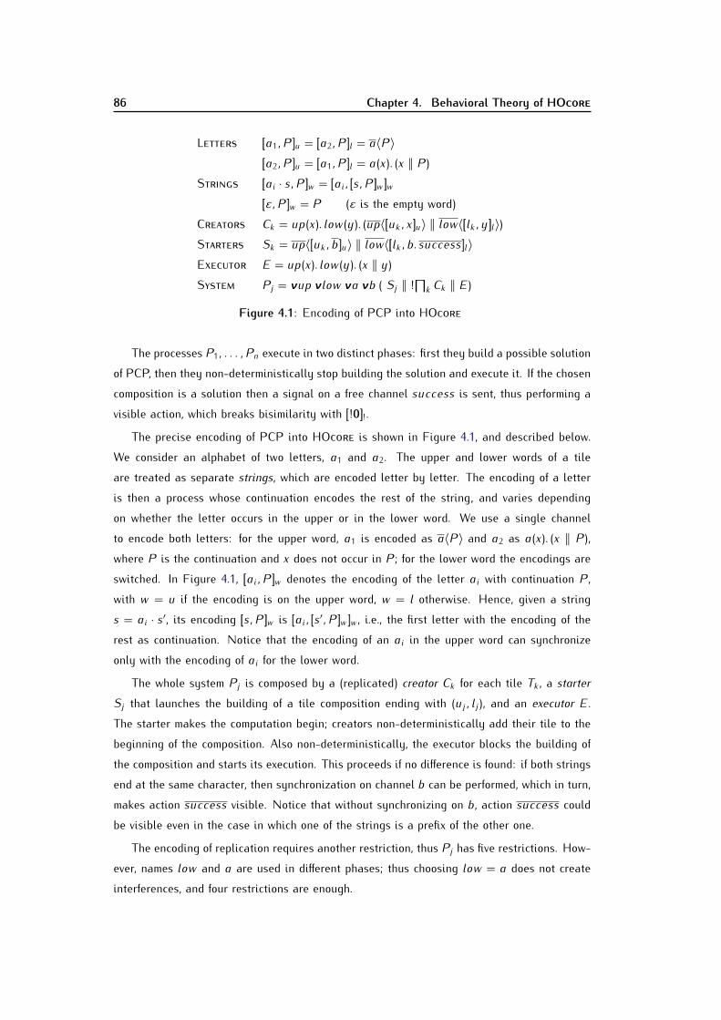
86 Chapter 4. Behavioral Theory of HOCORE
LETTERS [[a1, P]]u = [[a2, P]]l = a〈P〉[[a2, P]]u = [[a1, P]]l = a(x). (x ‖ P)STRINGS [[ai · s, P]]w = [[ai, [[s, P]]w ]]w[[ε, P]]w = P (ε is the empty word)CREATORS Ck = up(x). low(y). (up〈[[uk , x]]u〉 ‖ low〈[[lk , y]]l〉)STARTERS Sk = up〈[[uk , b]]u〉 ‖ low〈[[lk , b. success]]l〉EXECUTOR E = up(x). low(y). (x ‖ y)SYSTEM Pj = νup νlow νa νb ( Sj ‖ !∏k Ck ‖ E)Figure 4.1: Encoding of PCP into HOCORE
The processes P1, . . . , Pn execute in two distinct phases: first they build a possible solutionof PCP, then they non-deterministically stop building the solution and execute it. If the chosencomposition is a solution then a signal on a free channel success is sent, thus performing avisible action, which breaks bisimilarity with [[!0]]!.The precise encoding of PCP into HOCORE is shown in Figure 4.1, and described below.We consider an alphabet of two letters, a1 and a2. The upper and lower words of a tileare treated as separate strings, which are encoded letter by letter. The encoding of a letteris then a process whose continuation encodes the rest of the string, and varies dependingon whether the letter occurs in the upper or in the lower word. We use a single channelto encode both letters: for the upper word, a1 is encoded as a〈P〉 and a2 as a(x). (x ‖ P),where P is the continuation and x does not occur in P; for the lower word the encodings areswitched. In Figure 4.1, [[ai, P]]w denotes the encoding of the letter ai with continuation P,with w = u if the encoding is on the upper word, w = l otherwise. Hence, given a strings = ai · s′, its encoding [[s, P]]w is [[ai, [[s′, P]]w ]]w , i.e., the first letter with the encoding of therest as continuation. Notice that the encoding of an ai in the upper word can synchronizeonly with the encoding of ai for the lower word.The whole system Pj is composed by a (replicated) creator Ck for each tile Tk , a starterSj that launches the building of a tile composition ending with (uj , lj ), and an executor E .The starter makes the computation begin; creators non-deterministically add their tile to thebeginning of the composition. Also non-deterministically, the executor blocks the building ofthe composition and starts its execution. This proceeds if no difference is found: if both stringsend at the same character, then synchronization on channel b can be performed, which in turn,makes action success visible. Notice that without synchronizing on b, action success couldbe visible even in the case in which one of the strings is a prefix of the other one.The encoding of replication requires another restriction, thus Pj has five restrictions. How-ever, names low and a are used in different phases; thus choosing low = a does not createinterferences, and four restrictions are enough.

4.4. Bisimilarity is Undecidable with Four Static Restrictions 87
Theorem 4.3. Given an instance of PCP and one of its tiles Tj , there is a solution of theinstance of PCP ending with Tj iff Pj is not bisimilar to [[!0]]! according to any completeτ-bisimilarity.Proof. We start by proving the left to right implication. Note that [[!0]]! has a unique possiblecomputation, that is infinite and includes only τ actions. Let Ti1 , . . . , Tim be a solution ofthe instance of the PCP problem such that Tim = Tj . Then Pj can perform the computationdescribed below, which contains the action success, thus it is not bisimilar to [[!0]]!. Thecomputation is as follows:
1. Pj τ−→∗ νup, a, b. Sj ‖ ∏h=1..m−1 Cih ‖ ∏C ‖ ! ∏k Ck ‖ E = P ′1, by replication unfolding(the ∏C is the parallel composition of the creators that have been replicated and willnot be used);2. P ′1 τ−→∗ νup, a, b. up〈[[u, b]]u〉 ‖ a〈[[l, b. success]]l〉 ‖ ∏C ‖ ! ∏k Ck ‖ E = P ′2, where(u, l) is the solution of the instance of the PCP problem, by making the starter Sjinteract with the creators Cim−1 . .Ci1 ;3. P ′2 τ−→ τ−→ νup, a, b. ∏C ‖ ! ∏k Ck ‖ [[u, b]]u ‖ [[l, b. success]]l = P ′3, by making the starterinteract with the executor (note that as every creator starts by an input on up, none ofthem my be triggered by messages on a);4. P ′3 τ−→∗ νup, a, b. ∏C ‖ ! ∏k Ck ‖ b ‖ b. success = P ′4, by executing the encodings ofthe two strings, exploiting the fact that they are equal;5. P ′4 τ−→ νup, a, b. ∏C ‖ ! ∏k Ck ‖ success = P ′5, by synchronizing on b;6. P ′5 success−−−−−→ νup, a, b. ∏C ‖ ! ∏k Ck .For the other implication, first notice that all the computations of Pj are infinite since onecan always unfold recursion, and action success is the only possible visible action. Thusthe only possibility for having Pj not bisimilar to [[!0]]! is that Pj has a computation executingsuccess. The only computations that may produce success are structured as follows: theybuild two strings by concatenating the tiles, and then they execute them. One can prove byinduction on the minimum length of the strings that if the two strings are different then eithertheir execution gets stuck, or synchronization at b is not possible (this last case occurs if oneof the strings is a prefix of the other). Thus, the two strings must be equal and they are thesolution of the instance of the PCP problem.
Corollary 4.1. Barbed congruence and any complete τ-bisimilarity are undecidable in HOCOREwith four static restrictions.

88 Chapter 4. Behavioral Theory of HOCORE
Theorem 4.3 actually shows that even asynchronous barbed bisimilarity (defined as thelargest τ-bisimilarity that is output-barb preserving, and used in the definition of ordinaryasopposed to reduction-closedbarbed congruence) is undecidable. The corollary above thenfollows from the fact that all the relations there mentioned are at least as demanding asasynchronous barbed bisimilarity.4.5 Other Extensions
We now examine the impact on decidability of bisimilarity of some extensions of HOCORE. Weomit the details, including precise statements of the results.Abstractions. An abstraction is an expression of the form (x)P; it is a parametrized process.An abstraction has a functional type. Applying an abstraction (x)P of type T → ♦ (where ♦is the type of all processes) to an argument W of type T yields the process P{W/x}. Theargument W can itself be an abstraction; therefore the order of an abstraction, that is, thelevel of arrow nesting in its type, can be arbitrarily high. The order can also be ω, if there arerecursive types. By setting bounds on the order of the types of abstractions, one can definea hierarchy of subcalculi of the Higher-Order π-calculus (Sangiorgi and Walker, 2001); andwhen this bound is ω, one obtains a calculus capable of representing the π-calculus (for thisall operators of the Higher-Order π-calculus are needed, including full restriction).Allowing the communication of abstractions, as in the Higher-Order π-calculus, one thenalso needs to add in the grammar for processes an application construct of the form P1〈P2〉,as a destructor for abstractions. Extensions in the LTS would be as follows. Suppose, as in(Sangiorgi, 1996b), that beta-conversion � is the least precongruence on HOCORE processesgenerated by the rule (x)P1〈P2〉 � P1{P2/x}.The LTS could be then extended with a rule
BETA P � P ′1 P ′1 α−→ QP α−→ QNotice that with these additions, the characterization of bisimilarity as IO bisimilarity stillholds. For a HOCORE extended with abstractions and applications, ∼oIO is still a congruenceand is preserved by substitutions (by straighforward extensions of the proofs of Lemmas 4.2and 4.3). Note that, however, abstraction application may increase the size of processes. Ifabstractions are of finite type (i.e., their order is smaller than ω) then only a finite number ofsuch applications is possible, and decidability of bisimilarity is preserved. Decidability failsif the order is ω, intuitively because in this case it is possible to simulate the λ-calculus.

4.6. Concluding Remarks 89
Output prefix If we add an output prefix construct a〈P〉.Q to HOCORE, then the proof of thecharacterization as IO bisimilarity breaks and, with it, the proof of decidability. Decidabilityproofs can however be adjusted by appealing to results on unique decomposition of processesand axiomatization (along the lines of Section 4.3).Choice. Decidability remains with the addition of a choice operator to HOCORE. The proofsrequire little modifications. The addition of both choice and output prefix is harder. It might bepossible to extend the decidability proof for output prefix mentioned above so to accommodatealso choice, but the details become much more complex.Recursion. We do not know whether decidability is maintained by the addition of recursion(or similar operators such as replication).4.6 Concluding Remarks
Process calculi are usually Turing complete and have an undecidable bisimilarity (and barbedcongruence). Subcalculi have been studied where bisimilarity becomes decidable but then oneloses Turing completeness. Examples are BPA and BPP (see, e.g., (Kucera and Jancar, 2006))and CCS without restriction and relabeling (Christensen et al., 1994). In this chapter we haveshown that HOCORE is a Turing complete formalism for which bisimilarity is decidable. Wedo not know other concurrency formalisms where the same happens. Other peculiarities ofHOCORE are:1. it is higher-order, and contextual bisimilarities (barbed congruence) coincide with higher-order bisimilarity (as well as with others, such as context and normal bisimilarities); and2. it is asynchronous (in that there is no continuation underneath an output), yet asyn-chronous and synchronous bisimilarities coincide.
We do not know other non-trivial formalisms in which properties (1) or (2) hold (of course (1)makes sense only on higher-order models).We have also given an axiomatization for bisimilarity. From this we have derived polynomialupper bounds to the decidability of bisimilarity. The axiomatization also intuitively explainswhy results such as decidability, and the collapse of many forms of bisimilarity, are possibleeven though HOCORE is Turing complete: the bisimilarity relation is very discriminating.While in Chapter 3 we have used encodings of Minsky machines, here we have used encod-ings of the Post correspondence problem (PCP) for our undecidability results. The encodingsare tailored to analyze different problems: undecidability of termination, and undecidabilityof bisimilarity with static restrictions. The PCP encoding is always divergent, and therefore
90 Chapter 4. Behavioral Theory of HOCORE
cannot be used to reason about termination. On the other hand, the encoding of Minsky ma-chines would require at least one restriction for each instruction of the machine, and thereforewould have given us a (much) worse result for static restrictions. We find both encodingsinteresting: they show different ways to exploit higher-order communications for modeling.We have shown that bisimilarity becomes undecidable with the addition of four staticrestrictions. We do not know what happens with one, two, or three static restrictions. We alsodo not know whether the results presented would hold when one abstracts from τ-actions andmoves to weak equivalences. The problem seems much harder; it reminds us of the situation forBPA and BPP, where strong bisimilarity is decidable but the decidability of weak bisimilarityis a long-standing open problem (see, e.g., (Kucera and Jancar, 2006)).
Chapter 5
On the Expressiveness of Forwarding and
Suspension
In higher-order communication there are only two capabilities for received processes: executionand forwarding. In this chapter we aim at identifying the intrinsic souce of expressive power inHOCORE by studying a limited form of forwarding. Such a form is obtained from the followingsyntactic restriction: output actions can only communicate the parallel composition of knownclosed processes and processes received through previously executed input actions. We studythe expressiveness of HO−f , the fragment of HOCORE featuring this style of communication,using decidability of termination and convergence of processes as a yardstick. Our main resultshows that in HO−f termination is decidable while convergence is undecidable. Then, as away of recovering the expressiveness loss due to limited forwarding, we extend the calculuswith a form of process suspension called passivation. The resulting calculus is called HOP−f .Somewhat surprisingly, in HOP−f both termination and convergence are undecidable. Thisreveals a great deal of expressive power inherent to forms of suspension such as passivation.The chapter is structured as follows. The syntax and semantics of HO−f are introduced inSection 5.2. The encoding of Minsky machines into HO−f , and the undecidability of conver-gence are discussed in Section 5.3. The decidability of termination for HO−f is addressed inSection 5.4. The expressiveness results for HOP−f are presented in Section 5.5. Some finalremarks, as well as a review of related work, are included in Section 5.6.While the decidability results for HO−f have been previously presented as (Di Giustoet al., 2009a), the extension of HO−f with passivation and its associated decidability resultsare original to this dissertation.

92 Chapter 5. On the Expressiveness of Forwarding and Suspension
5.1 Introduction
Despite its minimality, in Chapter 3 HOCORE was shown to be Turing complete by exhibitingan encoding of Minsky machines.1 Therefore, properties such as• termination, i.e., non existence of divergent computations• convergence, i.e., existence of a terminating computation
are both undecidable in HOCORE2. In contrast, somewhat surprisingly, strong bisimilarity isdecidable, and several sensible bisimilarities coincide with it.In this chapter, we shall aim at identifying the intrinsic source of expressive power inHOCORE. A substantial part of the expressive power of a concurrent language comes from theability of accounting for infinite behavior. In higher-order process calculi there is no explicitoperator for such a behavior, as both recursion and replication can be encoded. We then findthat infinite behavior resides in the interplay of higher-order communication, in particular, inthe ability of forwarding a received process within an arbitrary context. For instance, considerthe process R = a(x).b〈Px〉, where Px stands for a process P with free occurrences of avariable x. Intuitively, R receives a process on name a and forwards it on name b. It is easyto see that since there are no limitations on the structure of objects in output actions, theactual structure of Px can be fairly complex. One could even “wrap” the process to be receivedin x using an arbitrary number of k “output layers”, i.e., by letting Px = b1〈b2〈. . . bk〈x〉〉 . . .〉.This nesting capability embodies a great deal of the expressiveness of HOCORE: as a matterof fact, the encoding of Minsky machines in HOCORE depends critically on nesting-basedcounters. Therefore, investigating suitable limitations to the kind of processes that can becommunicated in an output action appears as a legitimate approach to assess the expressivepower of higher-order concurrency.With the above consideration in mind, in this chapter we propose HO−f , a sublanguage ofHOCORE in which output actions are limited so as to rule out the nesting capability (Section5.2). In HO−f , output actions can communicate the parallel composition of two kinds of objects:1. closed processes (i.e., processes that do not contain free variables), and2. processes received through previously executed input actions.Hence, the context in which the output action resides can only contribute to communicationby “appending” pieces of code that admit no inspection, available in the form of a black-box.
1 Along the paper we use the appellations “Turing complete” and “weak Turing complete” as in the criteria definedby Bravetti and Zavattaro (2009) and discussed in Section 2.3.3.2Termination and convergence are sometimes also referred to as universal and existential termination, respectively.
5.1. Introduction 93
More precisely, the grammar of HO−f processes is the same as that of HOCORE, except for theproduction for output actions, which is replaced by the following one:a〈x1 ‖ · · · ‖ xk ‖ P〉where k ≥ 0 and P is a closed process. This modification directly restricts forwarding ca-pabilities for output processes, which in turn, leads to a more limited structure of processesalong reductions.The limited style of higher-order communication enforced in HO−f is relevant from a prag-matic perspective. In fact, communication in HO−f is inspired by those cases in which a processP is communicated in a translated format [[P]], and the translation is not compositional. Thatis, the cases in which, for any process context C , the translation of C [P] cannot be seen as afunction of the translation of P, i.e., there exists no context D such that [[C [P]]] = D[P].More concretely, communication as in HO−f can be related to several existing programmingscenarios. The simplest example is perhaps mobility of already compiled code, on which itis not possible to apply inverse translations (such as reverse engineering). Other examplesinclude proof-carrying code (Necula and Lee, 1998) and communication of obfuscated code(Collberg et al., 1998). The former features communication of executable code that comes witha certificate: a recipient can only check the certificate and decide whether to execute thecode or not. The latter consists of the communication of source code that is made difficult tounderstand for, e.g., security/copyright reasons, while preserving its functionality.In this chapter we study the expressiveness of HO−f using decidability of termination andconvergence of processes as a yardstick. Our main results are:
Undecidability of Convergence in HO−f . Similarly as in HOCORE, in HO−f it is possible toencode Minsky machines. The calculus thus retains a significant expressive power de-spite of the limited forwarding capability. Unlike HOCORE, however, HO−f is only weaklyTuring complete. In fact, the encoding of Minsky machines in HO−f is not faithful forit may introduce computations which do not correspond to the expected behavior of themodeled machine. Such computations are forced to be infinite and thus regarded asnon-halting computations which are therefore ignored. This allows us to prove that aMinsky machine terminates if and only if its encoding in HO−f converges. Consequently,convergence in HO−f is undecidable.Decidability of Termination in HO−f . In sharp contrast with HOCORE, termination in HO−f isdecidable. This result is obtained by appealing to the theory of well-structured transitionsystems (Finkel, 1990; Abdulla et al., 2000; Finkel and Schnoebelen, 2001), followingthe approach used by Busi et al. (2009). To the best of our knowledge, this is thefirst time the theory of well-structured transition systems is applied in a higher-orderconcurrency setting. This is significant because the adaptation to the HO−f case is

94 Chapter 5. On the Expressiveness of Forwarding and Suspension
far from trivial. Indeed, as we shall discuss, this approach relies on defining an upperbound on the depth of the (set of) derivatives of a process. By depth of a process wemean its maximal nesting of input/output actions. Notice that, even with the limitationon forwarding enforced by HO−f , because of the “term copying” feature of higher-ordercalculi, variable instantiation might lead to a potentially larger process. Hence, findingsuitable ways of bounding the set of derivatives of a process is rather challenging andneeds care.Undecidability of Termination and Convergence in HO−f with Passivation. The decidabilityof termination in HO−f provides compelling evidence on the fact that the limited forward-ing entails a loss of expressive power for HOCORE. It is therefore legitimate to investigatewhether such an expressive power can be recovered while preserving the essence of thelimited forwarding in HO−f . For this purpose, we extend HO−f with a passivation con-struct that allows to suspend the execution of a running process. Forms of processsuspension (such as passivation) are of both practical and theoretical interest as theyare at the heart of mechanisms for dynamic system reconfiguration. The extension ofHO−f with passivation, called HOP−f , is shown to be Turing complete by exhibiting afaithful encoding of Minsky machines. Therefore, in HOP−f both convergence and ter-mination are undecidable. To the best of our knowledge, ours is the first result on theexpressiveness and decidability of constructs for process suspension in the context ofhigher-order process calculi.5.2 The Calculus
We now introduce the syntax and semantics of HO−f . We use a, b, c to range over names, andx, y, z to range over variables; the sets of names and variables are disjoint.P, Q ::= a〈x1 ‖ · · · ‖ xk ‖ P〉 (with k ≥ 0, fv(P) = ∅) output| a(x).P input prefix| P ‖ Q parallel composition| x process variable| 0 nil
An input a(x).P binds the free occurrences of x in P. This is the only binder in the language.We write fv(P) and bv(P) for the set of free and bound variables in P, respectively. A processis closed if it does not have free variables. When x 6∈ fv(P), we abbreviate a(x).P as a.P. Wealso abbreviate a〈0〉 as a, P1 ‖ . . .‖Pk as ∏ki=1Pi, and omit trailing occurrences of 0. Hence,an output action can be written as a〈∏k∈K xk ‖P〉. We write ∏n1P as an abbreviation for the
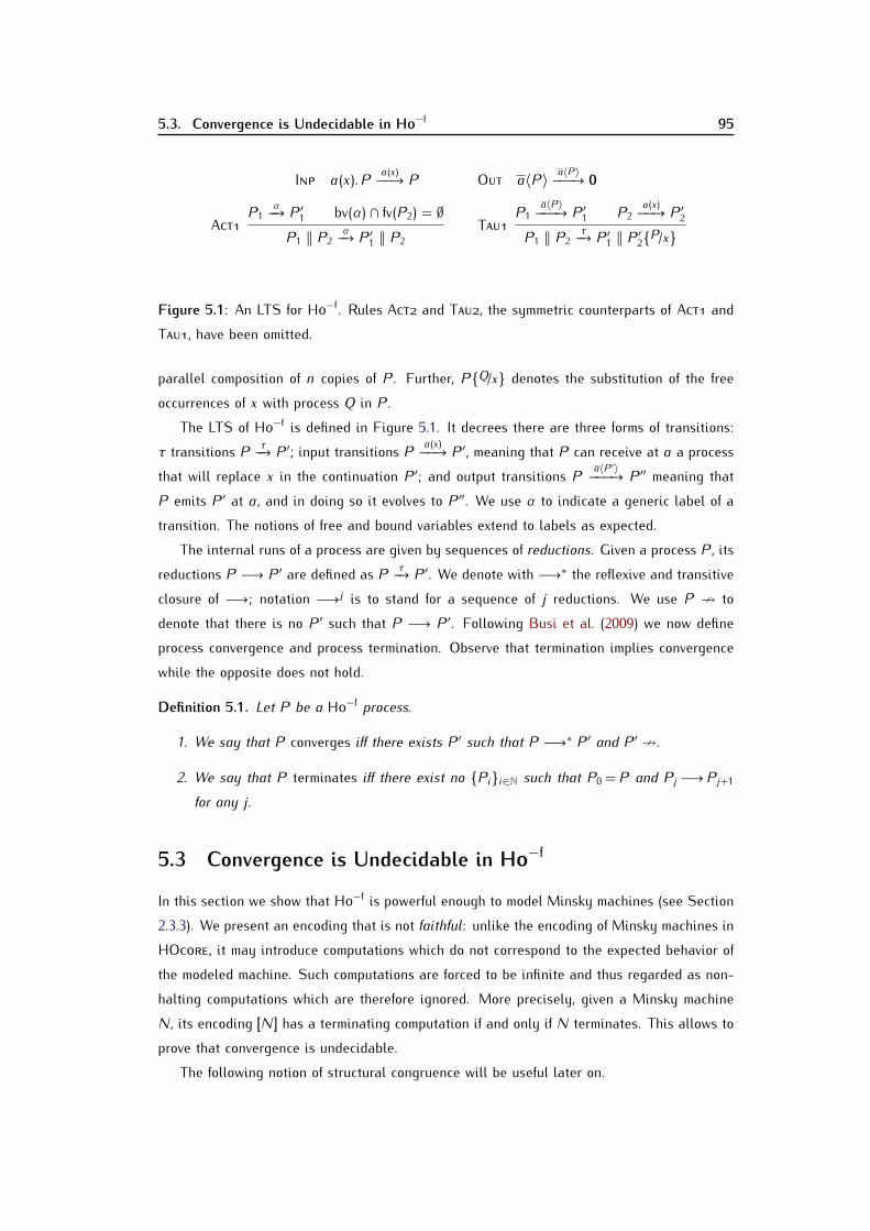
5.3. Convergence is Undecidable in HO−f 95
INP a(x).P a(x)−−→ P OUT a〈P〉 a〈P〉−−−→ 0
ACT1 P1 α−→ P ′1 bv(α) ∩ fv(P2) = ∅P1 ‖ P2 α−→ P ′1 ‖ P2 TAU1 P1 a〈P〉−−−→ P ′1 P2 a(x)−−→ P ′2P1 ‖ P2 τ−→ P ′1 ‖ P ′2{P/x}Figure 5.1: An LTS for HO−f . Rules ACT2 and TAU2, the symmetric counterparts of ACT1 andTAU1, have been omitted.parallel composition of n copies of P. Further, P{Q/x} denotes the substitution of the freeoccurrences of x with process Q in P.The LTS of HO−f is defined in Figure 5.1. It decrees there are three forms of transitions:τ transitions P τ−→ P ′; input transitions P a(x)−−→ P ′, meaning that P can receive at a a processthat will replace x in the continuation P ′; and output transitions P a〈P ′〉−−−→ P ′′ meaning thatP emits P ′ at a, and in doing so it evolves to P ′′. We use α to indicate a generic label of atransition. The notions of free and bound variables extend to labels as expected.The internal runs of a process are given by sequences of reductions. Given a process P, itsreductions P −→ P ′ are defined as P τ−→ P ′. We denote with −→∗ the reflexive and transitiveclosure of −→; notation −→j is to stand for a sequence of j reductions. We use P 9 todenote that there is no P ′ such that P −→ P ′. Following Busi et al. (2009) we now defineprocess convergence and process termination. Observe that termination implies convergencewhile the opposite does not hold.Definition 5.1. Let P be a HO−f process.
1. We say that P converges iff there exists P ′ such that P −→∗ P ′ and P ′ 9.2. We say that P terminates iff there exist no {Pi}i∈N such that P0 =P and Pj −→Pj+1for any j .
5.3 Convergence is Undecidable in HO−fIn this section we show that HO−f is powerful enough to model Minsky machines (see Section2.3.3). We present an encoding that is not faithful: unlike the encoding of Minsky machines inHOCORE, it may introduce computations which do not correspond to the expected behavior ofthe modeled machine. Such computations are forced to be infinite and thus regarded as non-halting computations which are therefore ignored. More precisely, given a Minsky machineN, its encoding [[N]] has a terminating computation if and only if N terminates. This allows toprove that convergence is undecidable.The following notion of structural congruence will be useful later on.

96 Chapter 5. On the Expressiveness of Forwarding and Suspension
REGISTER rj [[rj = m]]M = ∏m1 ujINSTRUCTIONS (i : Ii)[[(i : INC(rj ))]]M = !pi. (uj ‖ setj (x). (setj〈x ‖ INC〉 ‖ pi+1))[[(i : DECJ(rj , s))]]M = !pi. (loop ‖ uj . loop. setj (x). (setj〈x ‖ DEC〉 ‖ pi+1))‖ !pi. setj (x). (x ‖ setj〈x〉 ‖ ps)where INC = loop DEC = loop
Figure 5.2: Encoding of Minsky machines into HO−f
Definition 5.2. The structural congruence relation is the smallest congruence generated bythe following laws:P ‖ 0 ≡ P, P1 ‖ P2 ≡ P2 ‖ P1, P1 ‖ (P2 ‖ P3) ≡ (P1 ‖ P2) ‖ P3.
Lemma 5.1. If P α−→P ′ and P ≡ Q then there exists Q′ such that Q α−→Q′ and P ′ ≡ Q′.Proof. By induction on the derivation of P ≡ Q, then by case analysis on P α−→ Q.5.3.1 Encoding Minsky Machines into HO−fThe encoding of Minsky machines into HO−f is denoted by [[·]]M and presented in Figure 5.2.The encoding is assumed to execute in parallel with a process loop. DIV, which representsdivergent behavior that is spawned in certain cases with an output on name loop. This will bemade more precise later, when defining the encoding of a configuration of a Minsky machine.Before that, we begin by discussing the encodings of registers and instructions.A register rj that stores the number m is encoded as the parallel composition of m copiesof the unit process uj . To implement the test for zero it is necessary to record how manyincrements and decrements have been performed on the register rj . This is done by using aspecial process LOGj , which is communicated back and forth on name setj . More precisely,every time an increment instruction occurs, a new copy of the process uj is created, and theprocess LOGj is updated by adding the process INC in parallel. Similarly for decrements: acopy of uj is consumed and the process DEC is added to LOGj . As a result, after k incrementsand l decrements on register rj , we have that LOGj = ∏k INC ‖ ∏l DEC, which we abbreviateas LOGj [k, l].Each instruction (i : Ii) is a replicated process guarded by pi, which represents the programcounter when p = i. Once pi is consumed, the instruction is active and, in the case ofincrements and decrements, an interaction with a register occurs. We already described thebehavior of increments. Let us now focus on decrements, the instructions that can introduce
5.3. Convergence is Undecidable in HO−f 97
divergent unfaithful computations. In this case, the process can internally choose either toactually perform a decrement and proceed with the next instruction, or to jump. This internalchoice takes place on pi; it can be seen as a guess the process makes on the actual numberstored by the register rj . Therefore, two situations can occur:1. The process chooses to decrement rj . In this case a process loop as well as an input on ujbecome immediately available. The purpose of the latter is to produce a synchronizationwith a complementary output on uj (that represents a unit of rj ).If this operation succeeds (i.e., the guess is right as the content of rj is greater than 0)then a synchronization between the output loop available at the beginning and theinput on loop that guards the update of LOGj takes place. After this synchronization,the log of the register is updated (this is represented by two synchronizations on namesetj ) and instruction pi+1 is enabled.
Otherwise, if the synchronization on uj fails then it is because the content of rj is zeroand the process made a wrong guess. The process loop available at the beginning thensynchronizes with the external process loop. DIV, thus spawning a divergent computation.2. The process chooses to jump to instruction ps. In this case, the encoding checks if theactual value stored by rj is zero. To do so, the process receives the process LOGj on namesetj and launches it. The log contains a number of INC and DEC processes; dependingon the actual number of increments and decrements, two situations can occur.
In the first situation, the number of increments is equal to the number of decrements(say k); hence, the value of the rj is indeed zero and the process made a right guess. Inthis case, k synchronizations on name loop take place and instruction ps is enabled.In the second situation, the number of increments is greater than the number of decre-ments; hence, the value of rj is greater than zero and the process made a wrong guess. Asa result, at least one of the loop signals remains active; by means of a synchronizationthe process loop. DIV this is enough to to spawn a divergent computation.
Before executing the instructions, we require both registers in the Minsky machine to beset to zero. This is to guarantee correctness: starting with values different from zero in theregisters (without proper initialization of the logs) can lead to inconsistencies. For instance,the test for zero would succeed (i.e., without spawning a divergent computation) even for aregister whose value is different from zero.The following notation will be useful.Notation 5.1. Let N be a Minsky machine. The configuration (i, m0, m1) of N is annotatedas (i, mk0,l00 , mk1,l11 ), where, for j ∈ {0, 1}, kj and lj stand for the number of increments anddecrements performed on rj .

98 Chapter 5. On the Expressiveness of Forwarding and Suspension
Because we assume the value of both registers to be initialized with zero before executingthe instructions, the following is immediate.Fact 5.1. Let (i, mk0,l00 , mk1,l11 ) be an annotated Minsky configuration. We then have, for n ∈{0, 1}: (i) kn = ln if and only if rn = 0; and (ii) kn > ln if and only if rn > 0.
We are now ready to define the encoding of a configuration of the Minsky machine. Asmentioned before, the encodings of instructions and registers are put in parallel with a processthat spawns divergent behavior in case of a wrong guess.Definition 5.3 (Encoding of Configurations). Let N be a Minsky machine with registers r0, r1and instructions (1 : I1), . . . , (n : In). For j ∈ {0, 1}, suppose fresh, pairwise different namesrj , p1, . . . , pn, setj , loop, checkj . Also, let DIV be a divergent process (e.g. w ‖ !w.w). Giventhe encodings in Figure 5.2, we have:
1. The initial configuration (1, 00,0, 00,0) of N is encoded as:[[(1, 00,0, 00,0)]]M ::= p1 ‖ n∏
i=1 [[(i : Ii)]]M ‖ loop. DIV ‖ set0〈0〉 ‖ set1〈0〉 .2. A configuration (i, mk0,l00 , mk1,l11 ) of Nis encoded as:
[[(i, mk0,l00 , mk1,l11 )]]M = pi ‖ [[r0 = m0]]M ‖ [[r1 = m1]]M ‖ n∏i=1 [[(i : Ii)]]M ‖
loop. DIV ‖ set0〈LOG0[k0, l0]〉 ‖ set1〈LOG1[k1, l1]〉 .5.3.2 Correctness of the Encoding
We formalize the correctness of our encoding by means of two lemmas ensuring completeness(Lemma 5.2) and soundness (Lemma 5.3). Both these lemmas give us Theorem 5.1. We beginby formalizing the following intuition: removing the program counter from the encoding ofconfigurations leads to a stuck process.Proposition 5.1. Let N be a Minsky machine with registers r0, r1 and instructions (1 :I1), . . . , (n : In). Given the encodings in Figure 5.2, let P be defined as:
P = [[r0 = m0]]M ‖ [[r1 = m1]]M ‖ n∏i=1 [[(i : Ii)]]M ‖ loop. DIV ‖
set0〈LOG0[k0, l0]〉 ‖ set1〈LOG1[k1, l1]〉 .Then P 9.Proof. Straightforward by the following facts:
1. Processes [[r0 = m0]]M, [[r1 = m1]]M, set0〈LOG0[k0, l0]〉, and set1〈LOG1[k1, l1]〉 are outputactions that cannot evolve on their own.
5.3. Convergence is Undecidable in HO−f 99
2. For every i ∈ 1. .n, each [[(i : Ii)]]M is an input-guarded process, waiting for an activationsignal on pi.3. loop. DIV is an input-guarded process, and every output on loop appears guarded insidea decrement instruction.
Remark 5.1. Before entering into the proofs two remarks are in order. First, with a littleabuse of notation, we use notation Q 9 also for configurations of Minsky machines. Second,the encoding of input-guarded replication we have introduced here takes two reductions torelease a new copy of the guarded process (see Definition 3.5 and Lemma 3.1). However, forthe sake of simplicity, in proofs we shall denote only one of such reductions. In any case, itmust be taken into account that two reductions are required.We now state that the encoding is correct.
Lemma 5.2 (Completeness). Let (i, mk0,l00 , mk1,l11 ) be an (annotated) configuration of a Minskymachine N. Then, it holds:1. If (i, mk0,l00 , mk1,l11 ) 9 then [[(i, mk0,l00 , mk1,l11 )]]M 9
2. If (i, mk0,l00 , mk1,l11 ) −→M (i′, m′ k ′0,l′00 , m′ k ′1,l′11 ) then, for some P, [[(i, mk0,l00 , mk1,l11 )]]M −→∗ P ≡[[(i′, m′ k ′0,l′00 , m′ k ′1,l′11 )]]MProof. For (1) we have that if (i, mk0,l00 , mk1,l11 ) 9 then, by definition of Minsky machine, theprogram counter p is set to a non-existent instruction; i.e., for some i 6∈ [1. .n], p = i. Therefore,in process [[(i, mk0,l00 , mk1,l11 )]]M no instruction is guarded by pi. The thesis then follows as aneasy consequence of Proposition 5.1.For (2) we proceed by a case analysis on the instruction performed by N. Hence, wedistinguish three cases corresponding to the behaviors associated to rules M-JMP, M-DEC,and M-INC. Without loss of generality we assume instructions on register r0.Case M-INC We have a Minsky machine configuration (i, mk0,l00 , mk1,l11 ) with (i : INC(r0)). Bydefinition, its encoding into HO−f is as follows:
[[(i, mk0,l00 , mk1,l11 )]]M = pi ‖ [[r0 = m0]]M ‖ [[r1 = m1]]M ‖ ∏h=1..n,i 6=h[[(h : Ih)]]M ‖
!pi. (u0 ‖ set0(x). (set0〈x ‖ INC〉 ‖ pi+1)) ‖loop. DIV ‖ set0〈LOG0[k0, l0]〉 ‖ set1〈LOG1[k1, l1]〉We begin by noting that the program counter pi is consumed by the encoding of the in-struction i. As a result, process u0 is left unguarded; this represents the actual increment.We then have:

100 Chapter 5. On the Expressiveness of Forwarding and Suspension
[[(i, mk0,l00 , mk1,l11 )]]M −→≡ [[r0 = m0 + 1]]M ‖ set0(x). (set0〈x ‖ INC〉 ‖ pi+1) ‖set0〈LOG0[k0, l0]〉 ‖ S = Twhere S stands for the rest of the system, i.e.,
S = [[r1 = m1]]M ‖ n∏h=1[[(h : Ih)]]M ‖ loop. DIV ‖ set1〈LOG1[k1, l1]〉.
Now there is a synchronization on set0 for updating the log of register r0. This leavespi+1 unguarded, so the next instruction is enabled.T −→ pi+1 ‖ [[r0 = m0 + 1]]M ‖ [[r1 = m1]]M ‖ n∏
h=1[[(h : Ih)]]M ‖loop. DIV ‖ set0〈LOG0[k0 + 1, l0]〉 ‖ set1〈LOG1[k1, l1]〉 = T ′ .
We notice that T ′ ≡ [[(i+ 1, m0 + 1k0+1,l0 , mk1,l11 )]]M, as desired.Case M-DEC We have a Minsky machine configuration (i, mk0,l00 , mk1,l11 ) with r0 > 0 and (i :DECJ(r0, s)). By definition, its encoding into HO−f is as follows:
[[(i, mk0,l00 , mk1,l11 )]]M = pi ‖ [[r0 = m0]]M ‖ [[r1 = m1]]M ‖ ∏h=1..n,i6=h[[(h : Ih)]]M ‖
!pi. (loop ‖ u0. loop. set0(x). (set0〈x ‖ DEC〉 ‖ pi+1)) ‖!pi. set0(x). (x ‖ set0〈x〉 ‖ ps) ‖loop. DIV ‖ set0〈LOG0[k0, l0]〉 ‖ set1〈LOG1[k1, l1]〉In [[(i, mk0,l00 , mk1,l11 )]]M there is an internal choice on the program counter pi. This repre-sents a guess on the value of r0: pi can either synchronize with the first input-guardedprocess (so as to perform the actual decrement of the register) or with the second one(so as to perform a jump). Let us suppose that [[(i, mk0,l00 , mk1,l11 )]]M makes the right guessin this case, i.e., pi synchronizes with the first input-guarded process. We then have:
[[(i, mk0,l00 , mk1,l11 )]]M −→ [[r0 = m0]]M ‖loop ‖ u0. loop. set0(x). (set0〈x ‖ DEC〉 ‖ pi+1) ‖set0〈LOG0[k0, l0]〉 ‖ S = T1where S stands for the rest of the system, i.e.,
S = [[r1 = m1]]M ‖ n∏h=1[[(h : Ih)]]M ‖ loop. DIV ‖ set1〈LOG1[k1, l1]〉 ‖
!pi. set0(x). (x ‖ set0〈x〉 ‖ ps) .
5.3. Convergence is Undecidable in HO−f 101
Since we have assumed that r0 > 0, we are sure that a synchronization on u0 can takeplace, and thus the value of r0 decreases. Immediately after, there is also a synchro-nization on loop. More precisely, we haveT1 −→2 [[r0 = m0 − 1]]M ‖ set0(x). (set0〈x ‖ DEC0〉 ‖ pi+1) ‖ S = T2 .
Now the update of the log associated to r0 can take place, and a synchronization on set0is performed. As a result, the process pi+1 becomes unguarded and the next instructionis enabled:T2 −→≡ pi+1 ‖ [[r0 = m0 − 1]]M ‖ [[r1 = m1]]M ‖ n∏
h=1[[(h : Ih)]]M ‖loop. DIV ‖ set0〈LOG0[k0, l0 + 1]〉 ‖ set1〈LOG1[k1, l1]〉 = T3 .
Clearly, T3 ≡ [[(i+ 1, m0 − 1k0,l0+1, mk1,l11 )]]M, as desired.Case M-JMP This case is similar to the previous one. We have a Minsky machine configuration(i, mk0,l00 , mk1,l11 ) with (i : DECJ(r0, s)). In this case, m0 = 0. Hence, using Fact 5.1 wehave that k0 = l0.Again, we start from [[(i, mk0,l00 , mk1,l11 )]]M. There is an internal choice on the name pi. Letus suppose that [[(i, mk0,l00 , mk1,l11 )]]M makes the right guess, which in this case correspondsto the synchronization of pi and the second input-guarded process. We then have
[[(i, mk0,l00 , mk1,l11 )]]M −→ [[r0 = m0]]M ‖ set0(x). (x ‖ set0〈x〉 ‖ ps) ‖set0〈LOG0[k0, l0]〉 ‖ S′ = T1 .where S′ stands for the rest of the system, i.e.,
S = [[r1 = m1]]M ‖ n∏h=1[[(h : Ih)]]M ‖ loop. DIV ‖ set1〈LOG1[k1, l1]〉 ‖
!pi. (loop ‖ u0. loop. set0(x). (set0〈x ‖ DEC〉 ‖ pi+1)) .Now there is a synchronization on set0. As a result, the content of the log is left at thetop-level and hence executed. It is not lost, however, as it is still preserved inside anoutput on set0:
T1 −→≡ ps ‖ [[r0 = m0]]M ‖ [[r1 = m1]]M ‖ n∏h=1[[(h : Ih)]]M ‖
loop. DIV ‖ k0∏ INC ‖ l0∏ DEC ‖ set0〈LOG0[k0, l0]〉 ‖set1〈LOG1[k1, l1]〉 = T2 .

102 Chapter 5. On the Expressiveness of Forwarding and Suspension
Recall that k0 = l0. Starting in T2, we have that k0 synchronizations on loop take place;each of these corresponds to the interaction between a process INC and a correspondingprocess DEC. All of these processes are consumed. We then have that there exists a T3such that (i) T2 −→k0 T3 and (ii) T3 ≡ [[(s,mk0,l00 , mk1,l11 )]]M, as wanted.
Proposition 5.2. Let P0 = [[(i, rk0,l00 , rk1,l11 )]]M be the encoding of a Minsky machine configurationas in Definition 5.3, with (i : DEC(rj , s)) and kj > lj (for j ∈ {0, 1}).Suppose P0 −→∗ P such thatP ≡ [[r0 = m0]]M ‖ kj∏ INC ‖ lj∏ DEC ‖ set0〈LOG0[k0, l0]〉 ‖ ps ‖loop. DIV ‖ S
and where S is defined asS = [[r1 = m1]]M ‖ n∏
h=1[[(h : Ih)]]M ‖ set1〈LOG1[k1, l1]〉 ‖!pi. (loop ‖ u0. loop. set0(x). (set0〈x ‖ DEC〉 ‖ pi+1)) .
Then P does not converge.Proof (Sketch). Without loss of generality, we focus on the case in which j = 0 the proof isanalogous for j = 1 and assume that k0 = l0 + 1. The thesis follows by noticing that theonly possibilities for behavior are given by sub-processes ∏k0 INC, ∏l0 DEC, and loop. DIV ofP. In fact, using Definition 5.3 it is possible to infer all the other processes cannot reduce ontheir own. The same definition decrees that INC = loop and DEC = loop. It is easy to seethat divergent behavior can be spawned by any of the k0 occurrences of INC. Notice that thereis always at least one occurrence of INC ready to spawn divergency: even in the case someof such occurrences would reduce with corresponding input actions on loop, since k0 = l0 + 1in every computation there is at least an output loop ready to reduce with loop. DIV. Sinceno other process can reduce with the free loop, this means there is always a computationin which it reduces with the process loop. DIV. Hence, divergent behavior is spawned in allcases, and we are done.Lemma 5.3 (Soundness). Let (i, mk0,l00 , mk1,l11 ) be a configuration of a Minsky machine N. Given[[(i, mk0,l00 , mk1,l11 )]]M, for some n > 0 and process P ∈ HO−f , we have that:
1. If [[(i, mk0,l00 , mk1,l11 )]]M −→n P then either:• P ≡ [[(i′, m′k ′0,l′00 , m′k ′1,l′11 )]]M and (i, mk0,l00 , mk1,l11 ) −→M (i′, m′k ′0,l′00 , m′k ′1,l′11 ), or• P is a divergent process.

5.3. Convergence is Undecidable in HO−f 103
2. For all 0 ≤ m < n, if [[(i, mk0,l00 , mk1,l11 )]]M −→m P then, for some P ′, P −→ P ′.3. If [[(i, mk0,l00 , mk1,l11 )]]M 9 then (i, mk0,l00 , mk1,l11 ) 9.
Proof. For (1), since n > 0, in all cases there is at least one reduction from [[(i, m0, m1)]]M.An analysis of the structure of process [[(i, m0, m1)]]M reveals that, in all cases, the first stepcorresponds to the consumption of the program counter pi. This implies that there exists aninstruction labeled with i, that can be executed from the configuration (i, m0, m1). We proceedby a case analysis on the possible instruction, considering also the fact that the register onwhich the instruction acts can hold a value equal or greater than zero.Case i : INC(r0): Then the process evolves deterministically (up-to structural congruence) toP ≡ [[(i+ 1, m0 + 1, m1)]]M in n = 2 reductions. This is illustrated in the analogous casein the proof of Lemma 5.2(2).Case i : DEC(r0, s) with r0 > 0: We then have three main reduction sequences; one of themis finite, the other two are infinite. The finite reduction sequence is illustrated in theanalogous case in the proof of Lemma 5.2(2), where it is shown how [[(i, rk0,l00 , rk1,l11 )]]Mmay perform a sequence of n = 4 reductions that leads to [[(i+ 1, m0 − 1, m1)]]M.
The remaining (infinite) reduction sequences arise from the internal choice in pi thattakes place in [[(i, rk0,l00 , rk1,l11 )]]M. The first such sequences arises when pi synchronizeswith the first input-guarded replication on pi (the one implementing decrement); this isas in the analogous case in the proof of Lemma 5.2(2). This synchronization leads toprocess T1 in which the diverging computation arises from the synchronization betweenthe process loop and the process loop. DIV that spawns divergent behavior and is alwaysin parallel.The second infinite sequence arises when pi synchronizes with the second input-guardedreplication on pi (the one implementing jump). Notice that since r0 > 0, using Fact 5.1,we know that k0 > l0. It is sufficient to assume that k0 = l0 + 1. We have
[[(i, mk0,l00 , mk1,l11 )]]M −→ [[r0 = m0]]M ‖ set0(x). (x ‖ set0〈x〉 ‖ ps) ‖loop. DIV ‖ set0〈LOG0[k0, l0]〉 ‖ S = T1where S stands for the rest of the system, i.e.,
S = [[r1 = m1]]M ‖ n∏h=1[[(h : Ih)]]M ‖ set1〈LOG1[k1, l1]〉 ‖
!pi. (loop ‖ u0. loop. set0(x). (set0〈x ‖ DEC〉 ‖ pi+1)) .In T1 there is a synchronization on set0. Using the definition of LOG, we have:

104 Chapter 5. On the Expressiveness of Forwarding and Suspension
T1 −→ [[r0 = m0]]M ‖ l0+1∏ INC ‖ l0∏ DEC ‖ set0〈LOG0[k0, l0]〉 ‖ ps ‖loop. DIV ‖ S = T2 .The above puts us in the scenario of Proposition 5.2 which ensures that whenever aconfiguration in which the number of increments is greater or equal than the numberof decrements is reached (as in T2 above), the corresponding HO−f process does notconverge. This concludes the analysis for the case of decrement.
Case i : DEC(r0, s) with r0 = 0: Also in this case we have three main reduction sequences,one of them is finite, while the other two are infinite. The finite reduction sequenceis illustrated in the analogous case in the proof of Lemma 5.2(2), where it is shownhow [[(i, rk0,l00 , rk1,l11 )]]M may perform a sequence of n = 2 + l0 reductions that leads to[[(s,m0, m1)]]M.The two infinite reduction sequences arise similarly as in the previous case. The firstone arises after the two reduction steps that lead to process T3 in the analogous case inthe proof of Lemma 5.2(2). Indeed, only a single occurrence of process INC is sufficientto synchronize with process loop. DIV and to produce divergent behavior.The second infinite reduction sequence arises when the process makes a wrong guesson the content of the register. Again, we carry our analysis starting from process[[(i, mk0,l00 , mk1,l11 )]]M, given in the analogous case of the proof of Lemma 5.2(2). After thesynchronization on pi we have
[[(i, mk0,l00 , mk1,l11 )]]M −→ [[r0 = m0]]M ‖loop ‖ u0. loop. set0(x). (set0〈x ‖ DEC〉 ‖ pi+1) ‖set0〈LOG0[k0, l0]〉 ‖ loop. DIV ‖ S′ = T1where S′ is the rest of the system, i.e.
S′ = !mi. (set0(x). (x ‖ set0〈x〉 ‖ ps)) ‖ [[r1 = m1]]M ‖n∏h=1[[(h : Ih)]]M ‖ set1〈LOG1[k1, l1]〉.
It is easy to observe that since r0 = 0 there is no output on uj that can synchronize withthe input in T1. In fact, the only possible synchronization is on loop, which leaves thedivergent process unguarded. So we have that in two reduction steps [[(i, mk0,l00 , mk1,l11 )]]Mevolves into a diverging process, and the thesis holds.
5.4. Termination is Decidable in HO−f 105
Notice that statement (2) follows easily from the above analysis.As for (3), using Proposition 5.1 we know that if [[(i, m0, m1)]]M 9 then it is because pi isnot enabling any instruction. Hence, [[(i, m0, m1)]]M corresponds to the encoding of a haltinginstruction and we have that (i, m0, m1) 9, as desired.Summarizing Lemmas 5.2 and 5.3 we have the following:
Theorem 5.1. Let N be a Minsky machine with registers r0 = m0, r1 = m1, instructions(1 : I1), . . . , (n : In), and configuration (i, m0, m1). Then (i, m0, m1) terminates if and only ifprocess [[(i, m0, m1)]]M converges.As a consequence of the results above we have that convergence is undecidable.
Corollary 5.1. Convergence is undecidable in HO−f .5.4 Termination is Decidable in HO−fIn this section we prove that termination is decidable for HO−f processes. As hinted at inthe introduction, this is in sharp contrast with the analogous result for HOCORE. The proofappeals to the theory of well-structured transition systems, whose main definitions and resultswe summarize next.5.4.1 Well-Structured Transition Systems
The following results and definitions are from (Finkel and Schnoebelen, 2001), unless dif-ferently specified. Recall that a quasi-order (or, equivalently, preorder) is a reflexive andtransitive relation.Definition 5.4 (Well-quasi-order). A well-quasi-order (wqo) is a quasi-order ≤ over a setX such that, for any infinite sequence x0, x1, x2 . . . ∈ X , there exist indexes i < j such thatxi ≤ xj .
Note that if ≤ is a wqo then any infinite sequence x0, x1, x2, . . . contains an infinite in-creasing subsequence xi0 , xi1 , xi2 , . . . (with i0 < i1 < i2 < . . .). Thus well-quasi-orders excludethe possibility of having infinite strictly decreasing sequences.We also need a definition for (finitely branching) transition systems. This can be givenas follows. Here and in the following →∗ denotes the reflexive and transitive closure of therelation →.Definition 5.5 (Transition system). A transition system is a structure TS = (S,→), whereS is a set of states and →⊆ S × S is a set of transitions. We define Succ(s) as the set{s′ ∈ S | s → s′} of immediate successors of S. We say that TS is finitely branching if, foreach s ∈ S, Succ(s) is finite.

106 Chapter 5. On the Expressiveness of Forwarding and Suspension
The function Succ will also be used on sets by assuming the point-wise extension of theabove definitions. The key tool to decide several properties of computations is the notion ofwell-structured transition system. This is a transition system equipped with a well-quasi-order on states which is (upward) compatible with the transition relation. Here we will use astrong version of compatibility; hence the following definition.Definition 5.6 (Well-structured transition system). A well-structured transition system withstrong compatibility is a transition system TS = (S,→), equipped with a quasi-order ≤ onS, such that the two following conditions hold:
1. ≤ is a well-quasi-order;2. ≤ is strongly (upward) compatible with →, that is, for all s1 ≤ t1 and all transitionss1 → s2 , there exists a state t2 such that t1 → t2 and s2 ≤ t2 holds.The following theorem is a special case of Theorem 4.6 in (Finkel and Schnoebelen, 2001)and will be used to obtain our decidability result.
Theorem 5.2. Let TS = (S,→,≤) be a finitely branching, well-structured transition systemwith strong compatibility, decidable ≤, and computable Succ. Then the existence of an infinitecomputation starting from a state s ∈ S is decidable.We will also need a result due to Higman (1952) which allows to extend a well-quasi-orderfrom a set S to the set of the finite sequences on S. More precisely, given a set S let us denoteby S∗ the set of finite sequences built by using elements in S. We can define a quasi-orderon S∗ as follows.
Definition 5.7. Let S be a set and ≤ a quasi-order over S. The relation ≤∗ over S∗ is definedas follows. Let t, u ∈ S∗, with t = t1t2 . . . tm and u = u1u2 . . . un. We have that t ≤∗ u ifand only if there exists an injection f from {1, 2, . . . m} to {1, 2, . . . n} such that ti ≤ uf(i) andi ≤ f(i) for i = 1, . . . , m.The relation ≤∗ is clearly a quasi-order over S∗. It is also a wqo, since we have thefollowing result.
Lemma 5.4 (Higman (1952)). Let S be a set and ≤ a wqo over S. Then ≤∗ is a wqo over S∗.Finally we will use also the following proposition, whose proof is immediate.
Proposition 5.3. Let S be a finite set. Then the equality is a wqo over S.

5.4. Termination is Decidable in HO−f 107
INP a(x).P a(x)7−→ P OUT a〈P〉 a〈P〉7−→ 0
ACT1 P1 α7−→ P ′1P1 ‖ P2 α7−→ P ′1 ‖ P2 TAU1 P1 a〈P〉7−→ P ′1 P2 a(x)7−→ P ′2P1 ‖ P2 τ7−→ P ′1 ‖ P ′2{P/x}Figure 5.3: A finitely branching LTS for HO−f . Rules ACT2 and TAU2, the symmetric counter-parts of ACT1 and TAU1, have been omitted.5.4.2 A Finitely Branching LTS for HO−fIn order to exploit the theory of well-structured transition systems, a finitely branching LTS forHO−f is necessary. This is not a significant requirement in our case; the sensible issue hereis the treatment of alpha-conversion. To that end, we introduce an alternative LTS withoutalpha-conversion. As we shall see, since we restrict ourselves to closed processes and proofsfocus on internal synchronizations, the finitely branching LTS is equivalent to that introducedin Section 5.2. The alternative LTS is given in Figure 5.3; its most noticeable feature is theabsence of a side condition on rule ACT1.Lemma 5.5. Let P be a closed HO−f process. For every P ′ ∈ HO−f if P −→ P ′ then P ′ is aclosed process.Proof. By induction on the height of the inference tree for P −→ P ′ considering the possiblecases of the last step of the inference. There are four cases, corresponding to those relatedto rules TAU1, TAU2, ACT1, and ACT2. Let us focus only in the case in which TAU1 is the lastrule applied; the other cases are similar or simpler. Then P ≡ P1 ‖ P2 with P1 a〈R〉−−−−→ P ′1 andP2 a(x)−−−→ P ′2. Hence P1 ≡ a〈R〉 ‖ P ′1 and P2 ≡ a(x).P ′2. As such, P ′ ≡ P ′1 ‖ P ′2{R/x}. Weknow that P is a closed process; hence, both P ′1 and R are closed processes, and P ′2 is anopen process such that fn(P ′2) = {x}. Then the process P ′ is closed since it is equivalent tothe process P ′2 where all the free occurrences of the name x has been replaced with the closedprocess R .Remark 5.1. Notice that since in HO−f there is no restriction the only binder in the languageis the input prefix. Therefore, within a closed process P, the only non closed processes in Pare those occurring behind an input prefix, where they cannot evolve. By considering closedprocesses and restricting ourselves to reductions then α-conversion is not necessary.
As before, the internal runs of a process are given by sequences of reductions. Given aprocess P, its reductions in the alternative LTS P 7−→ P ′ are defined as P τ7−→ P ′. We denotewith 7−→∗ the reflexive and transitive closure of 7−→. We use P 67−→ to denote that there isno P ′ such that P 7−→ P ′.

108 Chapter 5. On the Expressiveness of Forwarding and Suspension
Given a process P, we shall use Pα to denote the result of applying the standard alpha-conversion without name captures over P.Lemma 5.6. Let P be a closed HO−f process. Then, P −→ P ′ iff P 7−→ P ′′ and P ′′ ≡ P ′α , forsome P ′ in HO−f .Proof. The “if” direction follows easily from Remark 5.1. The “only if” direction is straightfor-ward by observing that since P is a closed process, P ′′ is one of the possible evolutions of Pin −→.Corollary 5.2. Let P be a closed HO−f process. If P 7−→ P ′ then P ′ is a closed process inHO−f .Proof. Straightforward from Lemma 5.5 and Lemma 5.6.Corollary 5.3. Let P be a closed HO−f process. P 9 iff P 67−→.Proof. Straightforward from Lemma 5.6.Remark 5.2. The encoding of a Minsky machine presented in Section 5.3 is a closed process.Hence, all the results in that section hold for the LTS in Figure 5.3 as well.
The alphabet of an HO−f process is defined as follows:Definition 5.8 (Alphabet of a process). Let P be a HO−f process. The alphabet of P, denotedA(P), is inductively defined as:
A(0) = ∅ A(P ‖ Q) = A(P) ∪ A(Q) A(x) = {x}A(a(x).P) = {a, x} ∪ A(P) A(a〈P〉) = {a} ∪ A(P)
The following proposition can be shown for the alternative LTS because it does not consideralpha-conversion. As a matter of fact, had we considered open processes, we would haverequired α-conversion. In such a case, the inclusion A(P ′2{R/x}) ⊆ A(P ′2) ∪ A(R) would nolonger hold. This is because by using α-conversion during substitution some new variablescould be added to the alphabet.Proposition 5.4. Let P and P ′ be closed HO−f processes. If P 7−→ P ′ then A(P ′) ⊆ A(P).Proof. We proceed by a case analysis on the rule used to infer 7−→. We thus have four cases:Case TAU1 Then P = P1 ‖ P2 with P1 a〈R〉7−→ P ′1 and P2 a(x)7−→ P ′2. Hence P1 ≡ a〈R〉 ‖ P ′1, P2 ≡a(x).P ′2, and P ′ = P ′1 ‖ P ′2{R/x}. By Definition 5.8 we have that A(P1) = {a}∪A(P ′1)∪A(R) and hence A(P ′1) ⊆ A(P1). Also by Definition 5.8 we have A(P2) = {a, x}∪A(P ′2).Now, the process R is closed: therefore, during substitution, no variable can be captured.Hence, α-conversion is not needed, and we have A(P ′2{R/x}) ⊆ A(P ′2)∪A(R). The resultthen follows.

5.4. Termination is Decidable in HO−f 109
Case TAU2 Similarly as for TAU1.Case ACT1 Then P ≡ P1 ‖ P2, P ′ ≡ P ′1 ‖ P2, and P1 α7−→ P ′1. We then have A(P ′1) ⊆ A(P1)by using one of the above cases. By noting that A(P ′1) ∪ A(P2) ⊆ A(P1) ∪ A(P2), thethesis holds.Case ACT2 Similarly as for ACT1.
Fact 5.2. The LTS for HO−f given in Figure 5.3 is finitely branching.5.4.3 Termination is Decidable in HO−fHere we prove that termination is decidable in HO−f . The crux of the proof consists in findingan upper bound for a process and its derivatives. This is possible in HO−f because of thelimited structure allowed in output actions.We proceed as follows. First we define a notion of normal form for HO−f processes. Wethen characterize an upper bound for the derivatives of a given process, and define an orderingover them. This ordering is then shown to be a wqo that is strongly compatible with respect tothe LTS of HO−f given in Section 5.4.2. The decidability result is then obtained by resortingto the theory of well-structured transition systems introduced in Section 5.4.1.Definition 5.9 (Normal Form). Let P ∈ HO−f . P is in normal form iff
P = l∏k=1 xk ‖
m∏i=1 ai(yi).Pi ‖
n∏j=1 bj〈P ′j〉
where each Pi and P ′j are in normal form.Lemma 5.7. Every process P ∈ HO−f is structurally congruent to a normal form.Proof. By induction on the structure of P. The base cases are when P = 0 and when P = x,and are immediate. Cases P = a〈Q〉 and P = a(x).Q follow by applying the inductivehypothesis on Q. For the case P = P1 ‖ P2, we apply the inductive hypothesis twice and weobtain that
P1 ≡ l∏k=1 xk ‖
m∏i=1 ai(yi).Pi ‖
n∏j=1 bj〈Pj〉 and P2 ≡ l′∏
k=1 xk ‖m′∏i=1 a′i(y′i).P ′i ‖
n′∏j=1 b′j〈P ′j〉 .
It is then easy to see that P1 ‖ P2 is structurally congruent to a normal form, as desired.We now define an ordering over normal forms. Intuitively, a process is larger than anotherif it has more parallel components.

110 Chapter 5. On the Expressiveness of Forwarding and Suspension
Definition 5.10 (Relation �). Let P,Q ∈ HO−f . We write P � Q iff there exist x1 . . . xl,P1 . . . Pm, P ′1 . . . P ′n, Q1 . . . Qm, Q′1 . . . Q′n, and R such thatP ≡ ∏lk=1 xk ‖∏mi=1 ai(yi).Pi ‖∏nj=1 bj〈P ′j〉Q ≡ ∏lk=1 xk ‖∏mi=1 ai(yi).Qi ‖∏nj=1 bj〈Q′j〉 ‖ Rwith Pi � Qi and P ′j � Q′j , for i ∈ [1. .m] and j ∈ [1. .n].
The normal form of a process can be intuitively represented in a tree-like manner. Moreprecisely, given the process in normal formP = l∏
k=1 xk ‖m∏i=1 ai(yi).Pi ‖
n∏j=1 bj〈P ′j〉we shall decree its associated tree to have a root node labeled x1, . . . , xk . This root node hasm+n children, corresponding to the trees associated to processes P1, . . . , Pm and P ′1, . . . , P ′m;the outgoing edges connecting the root node and the children are labeled a1(y1), . . . , am(ym)and b1, . . . , bn.
Example 5.1. Process P = x ‖ a(y). (b.y ‖ c) ‖ a〈z ‖ d. e〉 has the following tree representa-tion:xa(y)
iiiiiii aUUUUUUU
•biiiiiii c
UUUUUUU zdy • •e•This intuitive representation of processes in normal form as trees will be useful to reasonabout the structure of HO−f terms. We begin by defining the depth of a process. Notice thatsuch a depth corresponds to the maximum depth of its tree representation.Definition 5.11 (Depth). Let P = ∏lk=1 xk ‖ ∏mi=1 ai(yi).Pi ‖ ∏nj=1 bj〈P ′j〉 be a HO−f processin normal form. The depth of P is given by
depth(P) = max{1 + depth(Pi), 1 + depth(P ′j ) | i ∈ [1. .m] ∧ j ∈ [1. .n]}.Given a natural number n and a process P, the set PP,n contains all those processes innormal form that can be built using the alphabet of P and whose depth is at most n.
Definition 5.12. Let n be a natural number and P ∈ HO−f . We define the set PP,n as follows:PP,n = {Q | Q ≡∏k∈K xk ‖∏i∈I ai(yi).Qi ‖∏j∈J bj〈Q′j〉∧ A(Q) ⊆ A(P)∧ Qi, Q′j ∈ PP,n−1 ∀i ∈ I, j ∈ J}where PP,0 contains processes that are built out only of variables in A(P).

5.4. Termination is Decidable in HO−f 111
As it will be shown later, the set of all derivatives of P is a subset of PP,2·depth(P).When compared to processes in languages such as CCS, higher-order processes have amore complex structure. This is because, by virtue of reductions, an arbitrary process cantake the place of possibly several occurrences of a single variable. As a consequence, thedepth of (the syntax tree of) a process cannot be determined (or even approximated) before itsexecution: it can vary arbitrarily along reductions. Crucially, in HO−f it is possible to boundsuch a depth. Our approach is the following: rather than solely depending on the depth of aprocess, we define measures on the relative position of variables within a process. Informallyspeaking, such a position will be determined by the number of prefixes guarding a variable.Since variables are allowed only at the top level of the output objects, their relative distancewill remain invariant during reductions. This allows to obtain a bound on the structure of HO−fprocesses. Finally, it is worth stressing that even if the same notions of normal form, depth,and distance can be defined for HOCORE, a finite upper bound for such a language does notexist.We first define the maximum distance between a variable and its binder.Definition 5.13. Let P = ∏k∈K xk ‖∏i∈I ai(yi).Pi ‖∏j∈J bj〈P ′j〉 be a HO−f process in normalform. We define the maximum distance of P as:
maxDistance(P) = max{maxDistyi (Pi), maxDistance(Pi),maxDistance(P ′j ) | i ∈ I, j ∈ J}where
maxDistx(P)=
1 if P = x,1 + maxDistx(Pz) if P = a(z).Pz ∧ x 6= z,1 + maxDistx(P ′) if P = a〈P ′〉,max{maxDistx(R),maxDistx(Q)} if P = R ‖ Q,0 otherwise.Lemma 5.8 (Properties of maxDistance). Let P be a closed HO−f process. It holds that:
1. maxDistance(P) ≤ depth(P)2. For every Q such that P 7−→ Q, maxDistance(Q) ≤ maxDistance(P).
Proof. Part (1) is immediate from Definitions 5.11 and 5.13. Part (2) follows by a case analysison the rule used to infer 7−→. We focus in the case TAU1: the other cases are similar or simpler.We then have that P = P1 ‖ P2 with P1 a〈S〉7−→ T and P2 a(x)7−→ R . Hence P1 ≡ a〈S〉 ‖ T and

112 Chapter 5. On the Expressiveness of Forwarding and Suspension
P2 ≡ a(x).R . We then have that P ≡ a〈S〉 ‖ T ‖ a(x).R and Q ≡ R{S/x} ‖ T . ApplyingDefinition 5.13 in both processes, we obtainmaxDistance(P) = max{maxDistance(S),maxDistx(R),maxDistance(R),maxDistance(T )}maxDistance(Q) = max{maxDistance(R{S/x}),maxDistance(T )} .
We can disregard the contribution of maxDistance(T ), since it does not participate in thesynchronization. We then focus on determining maxDistance(R{S/x}). Notice that the onlyway in which the value of maxDistance(R{S/x}) could be greater than that of maxDistance(R)is if S involves some free variables that get captured by an (input) binder in R by virtue ofthe substitution. Since S is a closed process, it has no free variables, and this capture is notpossible. Consequently, we havemaxDistance(R{S/x}) ≤ max{maxDistance(R),maxDistance(S)}
and the thesis holds.We now define the maximum depth of processes that can be communicated. Notice that thecontinuations of inputs are considered as along reductions they could become communicationobjects themselves:
Definition 5.14. Let P = ∏k∈K xk ‖∏i∈I ai(yi).Pi ‖∏j∈J bj〈P ′j〉 be a HO−f process in normalform. We define the maximum depth of a process that can be communicated (maxDepCom(P))in P as: maxDepCom(P) = max{maxDepCom(Pi), depth(P ′j ) | i ∈ I, j ∈ J} .Lemma 5.9 (Properties of maxDepCom). Let P be a closed HO−f process. It holds that:
1. maxDepCom(P) ≤ depth(P)2. For every Q such that P 7−→ Q, maxDepCom(Q) ≤ maxDepCom(P).
Proof. Part (1) is immediate from Definitions 5.11 and 5.14. Part (2) follows by a case analysison the rule used to infer 7−→. Again, we focus in the case TAU1: the other cases are similar orsimpler. We then have that P = P1 ‖ P2 with P1 a〈S〉7−→ T and P2 a(x)7−→ R . Hence P1 ≡ a〈S〉 ‖ Tand P2 ≡ a(x).R . We then have that P ≡ a〈S〉 ‖ T ‖ a(x).R and Q ≡ R{S/x} ‖ T . ApplyingDefinition 5.14 in both processes, we obtainmaxDepCom(P) = max{maxDepCom(T ),maxDepCom(S),maxDepCom(R), depth(S)}maxDepCom(Q) = max{maxDepCom(T ),maxDepCom(R{S/x})} .
5.4. Termination is Decidable in HO−f 113
We now focus on analyzing the influence a substitution has on communicated objects. Sincevariables can occur in output objects, the sensible case to check is if x appears inside somecommunication object in R . It is worth noticing that x is a variable that becomes free only asa result of the input on a, which consumes its binder. We thus have two cases:1. There are no communication objects in R with occurrences of x. Then, S will onlyoccur at the top level in R{S/x}. Since depth(S) was already taken into account whendetermining maxDepCom(P), we then have that maxDepCom(R{S/x}) ≤ maxDepCom(P),and the thesis holds.2. Some communication objects in R have occurrences of x. Then, R contains as sub-process an output message b〈Px〉 where, for some k > 0 and a closed process S′,process Px ≡ ∏k x ‖ S′. Process b〈Px{S/x}〉 then occurs in R{S/x}. Clearly, aneventual increase of maxDepCom(Q) depends on the depth of Px{S/x}. We have thatdepth(Px{S/x}) = max(depth(S), depth(S′)). Since both depth(S) and depth(S′) wereconsidered when determining maxDepCom(P), we conclude that maxDepCom(R{S/x})can be at most equal to maxDepCom(P), and so the thesis holds.
Generalizing Lemmas 5.8 and 5.9 we obtain:Corollary 5.4. Let P be a closed HO−f process. For every Q such that P 7−→∗ Q, it holdsthat:
1. maxDistance(Q) ≤ depth(P)2. maxDepCom(Q) ≤ depth(P).We are interested in characterizing the derivatives of a given process P. We shall showthat they are over-approximated by means of the set PP,2·depth(P). We will investigate theproperties of the relation � on such an approximation; such properties will also hold for theset of derivatives.
Definition 5.15. Let P ∈ HO−f . Then we define Deriv(P) = {Q | P 7−→∗ Q}The following results hold because of the limitations we have imposed on the output actionsfor HO−f processes.
Lemma 5.10. Let P,Q be HO−f processes such that A(Q) ⊆ A(P). Q ∈ PP,n if and only ifdepth(Q) ≤ n.
114 Chapter 5. On the Expressiveness of Forwarding and Suspension
Proof. The “if” direction is straightforward by definition of PP,n (Definition 5.12).For the “only if” direction we proceed by induction on n. If n = 0 then Q = 0 orQ = x1 ‖ · · · ‖ xk . In both cases, since A(Q) ⊆ A(P), Q is easily seen to be in PP,0. If n > 0then Q = ∏k∈K xk ‖
∏i∈I ai(yi).Qi ‖∏
j∈J bj〈Q′j〉where, for every i ∈ I and j ∈ J, both depth(Qi) ≤ depth(Q) ≤ n − 1 and depth(Q′j ) ≤depth(P) ≤ n− 1. By inductive hypothesis, each Qi and Q′j is in PP,n−1. Then, by Definition5.12, Q ∈ PP,n and we are done.Proposition 5.5. Let P be a HO−f process. Suppose, for some R and n, that P ∈ PR,n. Forevery Q such that P 7−→ Q, it holds that Q ∈ PR,2·n.Proof. We proceed by case analysis on the rule used to infer 7−→. We focus on the case sucha rule is TAU1; the remaining cases are similar or simpler. Recall that by Lemmas 5.8(1) and5.9(1) the maximum distance between an occurrence of a variable and its binder is bounded bydepth(P). By Definition 5.12 any process that can be communicated in P is in PR,n−1 and itsmaximum depth is also bounded by depth(P) which, in turn, by Lemma 5.10, is bounded byn. The deepest position for a variable is when it is a leaf in the tree associated to the normalform of P. That is, when its depth is exactly depth(P). If in that position we place a processin PR,n−1 whose depth is also depth(P) then it is easy to see that (the associated treeof) Q has a depth of 2 · depth(P), which is bounded by 2 · n. Hence, by Lemma 5.10, Q is inPR,2·n.
The lemma below generalizes Proposition 5.5 to a sequence of reductions.Lemma 5.11. Let P be a HO−f process. Suppose, for some R and n, that P ∈ PR,n. For everyQ such that P 7−→∗ Q, it holds that Q ∈ PR,2·n.Proof. The proof proceeds by induction on k , the length of 7−→∗, exploiting Proposition 5.5.The base case is when k = 1, and it follows by Proposition 5.5. For the inductive step weassume k > 1, so we have that, for some P ′, P 7−→∗ P ′ 7−→ Q where the sequence fromP to P ′ has lenght k − 1. By induction hypothesis we know that P ′ ∈ PR,2·n. We thenproceed by a case analysis on the rule used to infer P ′ 7−→ Q. As usual, we content ourselveswith illustrating the case TAU1; the other ones are similar or simpler. We then have thatP ′ = P1 ‖ P2 with P1 a〈T 〉7−→ S and P2 a(x)7−→ V . Hence P1 ≡ a〈T 〉 ‖ S and P2 ≡ a(x).V . Wethen have that P ′ ≡ a〈T 〉 ‖ S ‖ a(x).V and Q ≡ V{T/x} ‖ S.By Corollary 5.4 the maximum distance between x and its binder a(x) is depth(P), whichin turn is bounded by n (Lemma 5.10). Moreover, the maximum depth of T is bounded bymaxDepCom(P); by Corollary 5.4, depth(P) ≤ n. Therefore, the overall depth of process Q is2 · depth(P). Hence, and by using Lemma 5.10, Q ∈ RP,2·n, as wanted.
5.4. Termination is Decidable in HO−f 115
Corollary 5.5. Let P ∈ HO−f . Then Deriv(P) ⊆ PP,2·depth(P).We are now ready to prove that relation � is a wqo. We begin by showing that it is aquasi-order.
Proposition 5.6. The relation � is a quasi-order.Proof. We need to show that � is both reflexive and transitive. From Definition 5.9, reflexivityis immediate.Transitivity implies proving that, given processes P,Q, and R such that P � Q andQ � R , P � R holds. We proceed by induction on k = depth(P). If k = 0 then we havethat P = x1 ‖ · · · ‖ xk . Since P � Q, we have that Q = x1 ‖ · · · ‖ xk ‖ S. and thatR = x1 ‖ · · · ‖ xk ‖ S′, for some S, S′ such that S � S′. By Definition 5.10, the thesis follows.Now suppose k > 0. By Definition 5.9 and by hypothesis we have the following:
P = l∏k=1 xk ‖
m∏i=1 ai(yi).Pi ‖
n∏j=1 bj〈P ′j〉
Q = l∏k=1 xk ‖
m∏i=1 ai(yi).Qi ‖ n∏
j=1 bj〈Q′j〉 ‖ SR = l∏
k=1 xk ‖m∏i=1 ai(yi).Ri ‖
n∏j=1 bj〈R ′j 〉 ‖ S ‖ T .
with Pi � Qi, P ′j � Q′j , Qi � Ri, and Q′j � R ′j (i ∈ I, j ∈ J). Since Pi, P ′j , Qi, Q′j , Ri, and R ′jhave depth k − 1, by inductive hypothesis Pi � Ri and P ′j � R ′j . By Definition 5.10, the thesisfollows and we are done.We are now in place to state that � is a wqo.
Theorem 5.3 (Well-quasi-order). Let P ∈ HO−f be a closed process and n ≥ 0. The relation� is a well-quasi-order over PP,n.Proof. The proof is by induction on n.
• Let n=0. Then PP,0 contains processes made up only of variables taken from A(P). Theequality on finite sets is a well-quasi-ordering; by Lemma 5.4 (Higman’s Lemma) also=∗ is a well quasi-ordering: it corresponds to the ordering � on processes containingonly variables.• Let n>0. Take an infinite sequence of processes s=P1, P2, . . . , Pl, . . . with Pl∈PP,n.We shall show that the thesis holds by means of successive filterings of the normal formsof the processes in s. By Lemma 5.7 there exist Kl, Il and Jl such that
Pl ≡ ∏k∈Kl xk ‖
∏i∈Il ai(yi).Pli ‖∏
j∈Jl bj〈P ′lj 〉

116 Chapter 5. On the Expressiveness of Forwarding and Suspension
with Pli and P ′lj ∈ PP,n−1. Hence each Pl can be seen as composed of 3 finite sequences:(i) x1 . . . xk , (ii) a1(y1).Pl1 . . . ai(yi).Pli , and (iii) b1〈P ′l1 〉 . . . bj〈P ′lj 〉. We note that thefirst sequence is composed of variables from the finite set A(P) whereas the other twosequences are composed by elements in A(P) and PP,n−1. Since we have an infinitesequence of A(P)∗, as A(P) is finite, by Proposition 5.3 and Lemma 5.4 we have that=∗ is a wqo over A(P)∗.By inductive hypothesis, we have that � is a wqo on PP,n−1, hence by Lemma 5.4 relation�∗ is a wqo on P∗P,n−1. We start filtering out s by making the finite sequences x1 . . . xkincreasing with respect to =∗; let us call this subsequence t. Then we filter out t, bymaking the finite sequence a1(y1).Pl1 . . . ai(yi).Pli increasing with respect to both =∗and �∗. This is done in two steps: first, by considering the relation =∗ on the subjectof the actions (recalling that ai, yi ∈ A(P)), and second, by applying another filteringto the continuation using the inductive hypothesis. It is worth remarking that in the firststep we do not consider symbols of the alphabet but pairs of symbols. Since the set ofpairs on a finite set is still finite, we know by Higman’s Lemma that =∗ is a wqo on theset of sequences of pairs (ai, yi).For the sequence of outputs b1〈P ′l1 〉 . . . bj〈P ′lj 〉 this is also done in two steps: the subjectof the outputs are ordered with respect to =∗ and the objects of the output action areordered with respect to �∗ using the inductive hypothesis.At the end of the process we obtain an infinite subsequence of s that is ordered withrespect to �.
The last thing to show is that the well-quasi-ordering � is strongly compatible with respectto the LTS in Figure 5.3. We need some auxiliary results first.Lemma 5.12. Let P,P ′, Q and Q′ be HO−f processes in normal form such that P � P ′ andQ � Q′. Then it holds that P ‖ Q � P ′ ‖ Q′.Proof. Immediate from the definitions of normal form and � (Definitions 5.9 and 5.10).Lemma 5.13. Let P,P ′, Q, and Q′ be HO−f processes in normal form such that P � P ′ andQ � Q′. Then it holds that P{Q/x} � P ′{Q′/x}.Proof. By induction on the structure of P.
1. Cases P = 0 and P = y, for some y 6= x: Immediate.2. Case P = x. Then P ′ = x ‖ N, for some process N. We have that P{Q/x} = Q and thatP ′{Q′/x} = Q′ ‖ N{Q′/x}. Since Q � Q′ the thesis follows.

5.4. Termination is Decidable in HO−f 117
3. Case P = a(y).R . Then P ′ = a(y).R ′ ‖ N, for some process N. Since by hypothesisP � P ′, then R � R ′. We then have that P{Q/x} = a(y).R{Q/x} and that P ′{Q′/x} =a(y).R ′{Q/′}x ‖ N{Q′/x}. By inductive hypothesis we obtain that R{Q/x} � R ′{Q′/x},and the thesis follows.4. Case P = a〈R〉: Similar to (3).5. Case P = R ‖ S. Then P ′ = R ′ ‖ S′ ‖ N, for some process N, with R � R ′ and S � S′.We then have that P{Q/x} = R{Q/x} ‖ S{Q/x} and P ′{Q′/x} = R ′{Q′/x} ‖ S′{Q′/x} ‖N{Q′/x}. The thesis then follows by inductive hypothesis and Lemma 5.12.
Theorem 5.4 (Strong Compatibility). Let P,Q,P ′ ∈ HO−f . If P � Q and P 7−→ P ′ then thereexists Q′ such that Q 7−→ Q′ and P ′ � Q′.Proof. By case analysis on the rule used to infer reduction P 7−→ P ′. We content ourselveswith illustrating the case derived from the use of rule TAU1; the other ones are similar orsimpler. We then have that P = P ′ ‖ P ′′ with P ′ a〈P1〉7−→ N and P ′′ a(y)7−→ P2. Hence, P ≡ a〈P1〉 ‖a(y).P2 ‖ N. Since by hypothesis P � Q, we obtain a similar structure for Q. Indeed,Q ≡ a〈Q1〉 ‖ a(y).Q2 ‖ N′ with P1 � Q1, P2 � Q2, and N � N′.
Now, if P 7−→ P ′ ≡ P2{P1/y} ‖ N then also Q 7−→ Q′ ≡ Q2{Q1/y} ‖ N′. By Lemma 5.13we have P2{P1/y} � Q2{Q1/y}; using this and the hypothesis the thesis follows.Theorem 5.5. Let P ∈ HO−f be a closed process. The transition system (Deriv(P), 7−→,�) isa finitely branching well-structured transition system with strong compatibility, decidable �,and computable Succ.Proof. The transition system of HO−f is finitely branching (Fact 5.2). The fact that � is awell-quasi-order on Deriv(P) follows from Corollary 5.5 and Theorem 5.3. Strong compatibilityfollows from Theorem 5.4.
We can now state the main technical result of the section.Corollary 5.6. Let P ∈ HO−f be a closed process. Then, termination of P is decidable.Proof. This follows from Theorem 5.2, Theorem 5.5, and Corollary 5.3.
118 Chapter 5. On the Expressiveness of Forwarding and Suspension
5.5 On the Interplay of Fowarding and Passivation
The decidability of termination in HO−f presented in Section 5.4 provides compelling evidenceon the fact that the limited forwarding entails a loss of expressive power for HOCORE. Itis therefore worth investigating alternatives for recovering such an expressive power whilepreserving the essence of limited forwarding.In this section we examine one such alternatives. We analyze the consequences of extend-ing HO−f with a passivation construct, an operator that allows to suspend the execution of aprocess at run time. As such, it comes in handy to represent scenarios of (dynamic) systemreconfiguration, which are often indispensable in the specification of open, extensible systemssuch as component-based ones. Passivation has been considered by higher-order calculi suchas the Kell calculus (Schmitt and Stefani, 2004) and Homer (Hildebrandt et al., 2004), andfinds several applications (see, e.g., (Bundgaard et al., 2008)). Here we shall consider a passi-vation construct of the form a{P}, which represents a passivation unit named a that containsa process P. The passivation unit is a transparent locality, in that there are no restrictionson the interactions between P and processes surrounding a. The execution of P can be pas-sivated at an arbitrary time; this is represented by the evolution of a{P} into the nil processby means of an output action a〈P〉. Hence, the passivation of a{P} process might lead to asynchronization with any interacting input action on a.We consider HOP−f , the extension of HO−f with a passivation construct as described above.The syntax extends as expected; for the sake of consistency, we notice that the process P ina{P} respects the limitation on the shape of output objects introduced for HO−f . The LTSfor HOP−f is the same as that for HO−f in Section 5.2, extended with the two followingrules which formalize the intuitions given before with respect to transparent localities andpassivation, respectively:P α−−→ P ′a{P} α−−→ a{P ′} LOC a{P} a〈P〉−−−−→ 0 PAS .
5.5.1 A Faithful Encoding of Minsky Machines into HOP−fHere we investigate the expressiveness of HOP−f by exhibiting an encoding of Minsky machinesinto HOP−f . Interestingly, unlike the encoding presented in Section 5.3, the encoding intoHOP−f is faithful. As such, in HOP−f both termination and convergence are undecidableproblems. Hence, it is fair to say that the passivation construct even with the limitationon the shape of (output) processes allows to recover the expressive power lost in restrictingHOCORE as HO−f .The encoding is given in Figure 5.4; we now give some intuitions on it. A register kwith value m is represented by a passivation unit rk that contains the encoding of number

5.5. On the Interplay of Fowarding and Passivation 119
REGISTER rk [[rk = n]]M = rk{(| n |)k}where(| n |)k =
zk .az if n = 0uk . (a1 ‖ a2. (| n− 1 |)k ) if n > 0.INSTRUCTIONS (i : Ii)[[(i : INC(rk ))]]M = !pi. (rk (x). (ck〈x〉 ‖ rk{ck (y). (ap ‖ uk . (a1 ‖ a2.y))} ‖ ap.pi+1))[[(i : DECJ(rk , s))]]M = !pi. (m(x). x‖ d{uk ‖ a1.m〈s(x).d(x). (a2 ‖ pi+1)〉}‖ s{zk ‖ az .m〈d(x). s(x). rk (t). (rk{zk .az} ‖ ps)〉})
Figure 5.4: Encoding of Minsky machines into HOP−f .m, denoted (| m |)k . In turn, (| m |)k consists of a chain of m nested input prefixes on nameuk ; it also contains other prefixes on a1 and a2 which are used for synchronization purposesduring the execution of instructions. The encoding of zero is given by an input action on zkthat prefixes a trigger az .As expected, the encoding of an increment operation on the value of register k consistsin the enlargement of the chain of nested input prefixes it contains. For that purpose, thecontent of passivation unit rk is obtained with an input on rk . We therefore need to recreatethe passivation unit rk with the encoding of the incremented value. Notice that we requirean additional synchronization on ck in order to “inject” such a previous content in a newpassivation unit called rk . This way, the chain of nested inputs in rk can be enlarged whilerespecting the limitation on the shape of processes inside passivation units. As a result, thechain is enlarged by putting it behind some prefixes, and the next instruction can be invoked.This is done by a synchronization on name ap.The encoding of a decrement of the value of register k consists of an internal, exclusivechoice implemented as two passivation units that execute in parallel: the first one, named d,implements the behavior for decrementing the value of a register, while the second one, nameds, implements the behavior for performing the jump to some given instruction. Unlike theencoding of Minsky machines in HO−f presented in Section 5.3, this internal choice behavesfaithfully with respect to the encoding instruction, i.e., the behavior inside d will only executeif the value in rk is greater than zero, whereas the behavior inside s will only execute ifthat value is equal to zero. It is indeed a deterministic choice in that it is not the case thatboth an input prefix on uk (which triggers the “decrement branch” defined by d) and one onzk (which triggers the “jump branch” defined by s) are available at the same time; this isbecause of the way in which we encode numbers, i.e., as a chain of input prefixes. In addition

120 Chapter 5. On the Expressiveness of Forwarding and Suspension
to the passivation units, the encoding of decrement features a “manager” (implemented as asynchronization on m) that enables the behavior of the chosen passivation unit by placing it atthe top-level, and consumes both s and d afterwards, thus leaving no residual processes afterperforming the instruction. In case the value of the register is equal to some n > 0, then adecrement is implemented by consuming the input prefixes on uk and a2 and the output prefixon a1 through suitable synchronizations. It is worth noticing that these synchronizatons areonly possible because the passivation units containing the encoding of n behave as transparentlocalities, and hence able to interact with its surrounding context. As a result, the encodingof n− 1 remains inside rk and the next instruction is invoked. In case the value of the registeris equal to zero, the passivation unit rk is consumed and recreated with the encoding of zeroinside. The jump is then performed by invoking the respective instruction.We are now ready to define the encoding of a configuration of a Minsky machine intoHOP−f .Definition 5.16 (Encoding of Configurations). Let N be a Minsky machine with registersr0 = m0, r1 = m1 and instructions (1 : I1), . . . , (n : In). The encoding of a configuration(i, m0, m1) of N into HOP−f is defined by the encodings in Figure 5.4 as
[[(i, m0, m1)]]M = pi ‖ [[r0 = m0]]M ‖ [[r1 = m1]]M ‖ n∏i=1 [[(i : Ii)]]M ,
assuming fresh, pairwise different names rj , uk , zk , p1, . . . , pn, (for j ∈ {0, 1}).5.5.2 Correctness of the Encoding
We divide the proof of correctness into two properties: completeness (Lemma 5.14) and sound-ness (Lemma 5.15).Lemma 5.14 (Completeness). Let (i, m0, m1) be a configuration of a Minsky machine N.Then, if (i, m0, m1) −→M (i′, m′0, m′1) then, for some finite j and a process P, it holds that[[(i, m0, m1)]]M −→j P ≡ [[(i′, m′0, m′1)]]M.Proof. We proceed by a case analysis on the instruction performed by the Minsky machine.Hence, we distinguish three cases corresponding to the behaviors associated to rules M-INC,M-DEC, and M-JMP. Without loss of generality, we restrict our analysis to operations onregister r0.Case M-INC: We have a Minsky configuration (i, m0, m1) with (i : INC(r0)). By Definition5.16, its encoding into HO−f with passivation is as follows:
[[(i, m0, m1)]]M = pi ‖ [[r0 = m0]]M ‖ [[r1 = m1]]M ‖[[(i : INC(r0))]]M ‖ ∏l=1..n,l6=i[[(l : Il)]]M
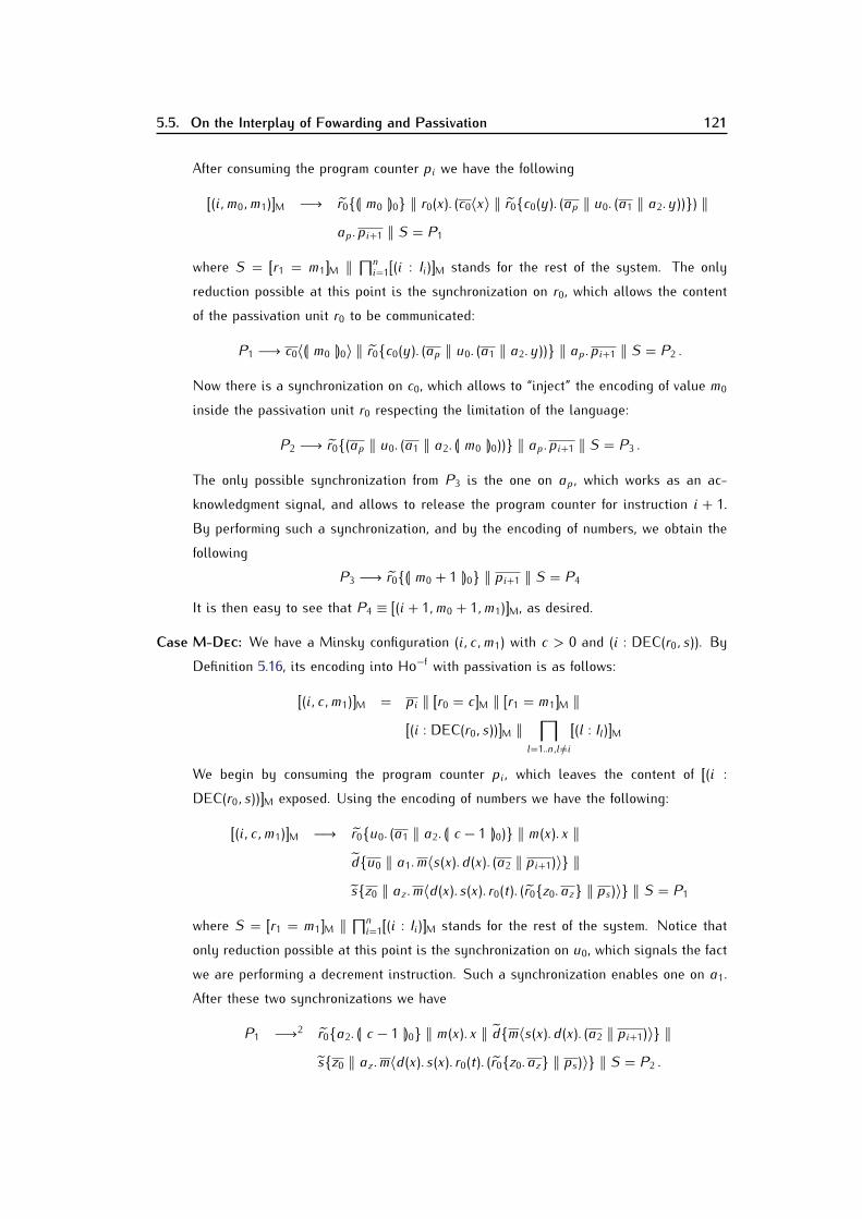
5.5. On the Interplay of Fowarding and Passivation 121
After consuming the program counter pi we have the following[[(i, m0, m1)]]M −→ r0{(| m0 |)0} ‖ r0(x). (c0〈x〉 ‖ r0{c0(y). (ap ‖ u0. (a1 ‖ a2.y))}) ‖ap.pi+1 ‖ S = P1
where S = [[r1 = m1]]M ‖ ∏ni=1[[(i : Ii)]]M stands for the rest of the system. The onlyreduction possible at this point is the synchronization on r0, which allows the contentof the passivation unit r0 to be communicated:P1 −→ c0〈(| m0 |)0〉 ‖ r0{c0(y). (ap ‖ u0. (a1 ‖ a2.y))} ‖ ap.pi+1 ‖ S = P2 .
Now there is a synchronization on c0, which allows to “inject” the encoding of value m0inside the passivation unit r0 respecting the limitation of the language:P2 −→ r0{(ap ‖ u0. (a1 ‖ a2. (| m0 |)0))} ‖ ap.pi+1 ‖ S = P3 .
The only possible synchronization from P3 is the one on ap, which works as an ac-knowledgment signal, and allows to release the program counter for instruction i + 1.By performing such a synchronization, and by the encoding of numbers, we obtain thefollowing P3 −→ r0{(| m0 + 1 |)0} ‖ pi+1 ‖ S = P4It is then easy to see that P4 ≡ [[(i+ 1, m0 + 1, m1)]]M, as desired.Case M-DEC: We have a Minsky configuration (i, c,m1) with c > 0 and (i : DEC(r0, s)). ByDefinition 5.16, its encoding into HO−f with passivation is as follows:
[[(i, c,m1)]]M = pi ‖ [[r0 = c]]M ‖ [[r1 = m1]]M ‖[[(i : DEC(r0, s))]]M ‖ ∏l=1..n,l 6=i[[(l : Il)]]M
We begin by consuming the program counter pi, which leaves the content of [[(i :DEC(r0, s))]]M exposed. Using the encoding of numbers we have the following:[[(i, c,m1)]]M −→ r0{u0. (a1 ‖ a2. (| c − 1 |)0)} ‖ m(x). x ‖d{u0 ‖ a1.m〈s(x).d(x). (a2 ‖ pi+1)〉} ‖s{z0 ‖ az .m〈d(x). s(x). r0(t). (r0{z0.az} ‖ ps)〉} ‖ S = P1
where S = [[r1 = m1]]M ‖ ∏ni=1[[(i : Ii)]]M stands for the rest of the system. Notice thatonly reduction possible at this point is the synchronization on u0, which signals the factwe are performing a decrement instruction. Such a synchronization enables one on a1.After these two synchronizations we haveP1 −→2 r0{a2. (| c − 1 |)0} ‖ m(x). x ‖ d{m〈s(x).d(x). (a2 ‖ pi+1)〉} ‖s{z0 ‖ az .m〈d(x). s(x). r0(t). (r0{z0.az} ‖ ps)〉} ‖ S = P2 .
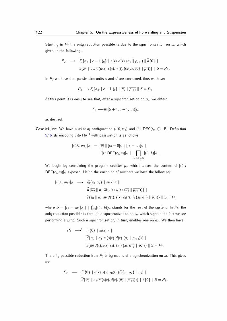
122 Chapter 5. On the Expressiveness of Forwarding and Suspension
Starting in P2 the only reduction possible is due to the synchronization on m, whichgives us the following:P2 −→ r0{a2. (| c − 1 |)0} ‖ s(x).d(x). (a2 ‖ pi+1) ‖ d{0} ‖s{z0 ‖ az .m〈d(x). s(x). r0(t). (r0{z0.az} ‖ ps)〉} ‖ S = P3 .
In P3 we have that passivation units s and d are consumed, thus we have:P3 −→ r0{a2. (| c − 1 |)0} ‖ a2 ‖ pi+1 ‖ S = P4 .
At this point it is easy to see that, after a synchronization on a2, we obtainP4 −→≡ [[(i+ 1, c − 1, m1)]]M
as desired.Case M-JMP: We have a Minsky configuration (i, 0, m1) and (i : DEC(r0, s)). By Definition5.16, its encoding into HO−f with passivation is as follows:
[[(i, 0, m1)]]M = pi ‖ [[r0 = 0]]M ‖ [[r1 = m1]]M ‖[[(i : DEC(r0, s))]]M ‖ ∏l=1..n,l 6=i[[(l : Il)]]M .
We begin by consuming the program counter pi, which leaves the content of [[(i :DEC(r0, s))]]M exposed. Using the encoding of numbers we have the following:[[(i, 0, m1)]]M −→ r0{z0.az} ‖ m(x). x ‖d{u0 ‖ a1.m〈s(x).d(x). (a2 ‖ pi+1)〉} ‖s{z0 ‖ az .m〈d(x). s(x). r0(t). (r0{z0.az} ‖ ps)〉} ‖ S = P1
where S = [[r1 = m1]]M ‖ ∏ni=1[[(i : Ii)]]M stands for the rest of the system. In P1, theonly reduction possible is through a synchronization on z0, which signals the fact we areperforming a jump. Such a synchronization, in turn, enables one on az . We then have:P1 −→2 r0{0} ‖ m(x). x ‖d{u0 ‖ a1.m〈s(x).d(x). (a2 ‖ pi+1)〉} ‖s{m〈d(x). s(x). r0(t). (r0{z0.az} ‖ ps)〉} ‖ S = P2 .
The only possible reduction from P2 is by means of a synchronization on m. This givesus:P2 −→ r0{0} ‖ d(x). s(x). r0(t). (r0{z0.az} ‖ ps) ‖d{u0 ‖ a1.m〈s(x).d(x). (a2 ‖ pi+1)〉} ‖ s{0} ‖ S = P3 .

5.6. Concluding Remarks 123
In P3 the two passivation units on d and s are consumed, which gives us:P3 −→ r0{0} ‖ r0(t). (r0{z0.az} ‖ ps) ‖ S = P4 .
At this point, it is easy to see that after a synchronization on r0 we obtain:P4 −→≡ [[(s, 0, m1)]]M
as desired.
Lemma 5.15 (Soundness). Let (i, m0, m1) be a configuration of a Minsky machine N.If [[(i, m0, m1)]]M −→ P1 then for every computation of P1 there exists a Pj such that Pj =[[(i′, m′0, m′1)]]M and (i, m0, m1) −→M (i′, m′0, m′1).Proof. Consider the reduction [[(i, m0, m1)]]M −→ P1. An analysis of the structure of process[[(i, m0, m1)]]M reveals that, in all cases, the only possibility for the first step corresponds to theconsumption of the program counter pi. This implies that there exists an instruction labeledwith i, that can be executed from the configuration (i, m0, m1). We proceed by a case analysison the possible instruction, considering also the fact that the register on which the instructionacts can hold a value equal or greater than zero.In all cases, it can be shown that computation evolves deterministically until reaching aprocess in which a new program counter (that is, some pi′ ) appears. The program counter pi′ isalways inside a process that corresponds to [[(i′, m′0, m′1)]]M, where (i, m0, m1) −→M (i′, m′0, m′1).The detailed analysis follows the same lines as the one reported for the proof of Lemma 5.14,and we omit it.Corollary 5.7. Let N be a Minsky machine. We have that N 9M if and only if [[N]]M 9.Proof. Straightforward from Lemmas 5.14 and 5.15.Lemma 5.16. Termination and convergence are undecidable in HOP−f .Proof. This is an immediate consequence of previous results (Lemmas 5.14 and 5.15, Corollary5.7).5.6 Concluding Remarks
In this chapter we have studied the expressiveness and decidability of higher-order processcalculi featuring limited forwarding. Our study has been centered around HO−f , the fragment ofHOCORE in which output actions can only include previously received processes in compositionwith closed ones. This communication style is reminiscent of programming scenarios with forms

124 Chapter 5. On the Expressiveness of Forwarding and Suspension
of code mobility in which the recipient is not authorized or capable of accessing/modifyingthe structure of the received code. We have shown that such a weakening of the forwardcapabilities of higher-order processes has consequences both on the expressiveness of thelanguage and on the decidability of termination. Furthermore, we analyzed the extension ofHO−f with a passivation operator as a way of recovering the expressive power lost when movingfrom HOCORE to HO−f .By exhibiting an encoding of Minsky machines into HO−f , we have shown that convergenceis undecidable. Unlike the encoding of Minsky machines in HOCORE presented in Chapter 3,the encoding in HO−f is not faithful. Hence, in the terminology of Bravetti and Zavattaro (2009),while HOCORE is Turing complete, HO−f is only weakly Turing complete. This discrepancyon the criteria satisfied by each encoding reveals an expressiveness gap between HO−f andHOCORE; nevertheless, it seems clear that the loss of expressiveness resulting from limiting theforwarding capabilities in HOCORE is much less dramatic than what one would have expected.We have shown that the communication style of HO−f causes a separation result with re-spect to HOCORE. In fact, because of the limitation on output actions, it was possible to provethat termination in HO−f is decidable. This is in sharp contrast with the situation in HOCORE,for which termination is undecidable. In HO−f , it is possible to provide an upper bound on thedepth (i.e., the level of nesting of actions) of the (set of) derivatives of a process. In HOCOREsuch an upper bound does not exist. This was shown to be essential for obtaining the decid-ability result; for this, we appealed to the approach developed in (Busi et al., 2009), whichrelies on the theory of well-structured transition systems (Finkel, 1990; Abdulla et al., 2000;Finkel and Schnoebelen, 2001). As far as we are aware, this approach to studying expres-siveness issues has not previously been used in the higher-order setting. The decidability oftermination is significant, as it might shed light on the development of verification techniquesfor higher-order processes.We have also studied the expressiveness and decidability of HOP−f , the extension of HO−f
with a passivation operator. To the best of our knowledge, this is the first expressiveness studyinvolving passivation operators in the context of higher-order process calculi. In HOP−f it ispossible to encode Minsky machines in a faithful manner. Hence, similarly as in HOCORE, inHOP−f both termination and convergence are undecidable. This certainly does not imply thatboth languages have the same expressive power; in fact, an interesting direction for future workconsists in assessing the exact expressive power that passivation brings into the picture. Thiswould include not only a comparison between HOP−f and HOCORE, but also a comparisonbetween HOCORE and HOCORE extended with passivation. All the languages involved areTuring complete, hence such comparisons should employ techniques different from the onesused here. It is also worth remarking that we have considered a very simple form of passivation,one in which process suspension takes place with a considerable degree of non-determinism.

5.6. Concluding Remarks 125
Studying other forms of passivation, possibly with more explicit control mechanisms, could beinteresting from several points of view, including expressiveness.The HO−f calculus is a sublanguage of HOCORE. As such, HO−f inherits the many resultsand properties of HOCORE; most notably, a notion of (strong) bisimilarity which is decidable andcoincides with a number of sensible equivalences in the higher-order context. Our results thuscomplement those in previous chapters and deepen our understanding of the expressiveness ofcore higher-order calculi as a whole. Furthermore, by recalling that CCS without restriction isnot Turing complete and has decidable convergence, the present results shape an interestingexpressiveness hierarchy, namely one in which HOCORE is strictly more expressive than HO−f(because of the discussion above), and in which HO−f is strictly more expressive than CCSwithout restriction.Remarkably, our undecidability result can be used to prove that (weak) barbed bisimilarityis undecidable in the calculus obtained by extending HO−f with restriction. Consider theencoding of Minsky machines used in Section 5.3 to prove the undecidability of convergencein HO−f . Consider now the restriction operator (νx) used as a binder for the names in thetuple x. Take a Minsky machine N (it is not restrictive to assume that it executes at least oneincrement instruction) and its encoding P, as given by Definition 5.3. Let x be the tuple ofthe names used by P, excluding the name w. We have that N terminates if and only if (νx)Pis (weakly) barbed equivalent to the process (νd)(d | d | d. (w | !w.w)).Related Work. We do not know of other works that study the expressiveness of higher-ordercalculi by restricting higher-order outputs. The recent work (Bundgaard et al., 2009) studiesfinite-control fragments of Homer (Hildebrandt et al., 2004), a higher-order process calculuswith locations. While we have focused on decidability of termination and convergence, in(Bundgaard et al., 2009) the interest is in decidability of barbed bisimilarity. One of theapproaches explored in (Bundgaard et al., 2009) is based on a type system that bounds thesize of processes in terms of their syntactic components (e.g. number of parallel components,location nesting). Although the restrictions such a type system imposes might be considered assimilar in spirit to the limitation on outputs in HO−f (in particular, location nesting resemblesthe output nesting HO−f forbids), the fact that the synchronization discipline in Homer dependsheavily on the structure of locations makes it difficult to establish a more detailed comparisonwith HO−f .Also similar in spirit to our work, but in a slightly different context, are some studieson the expressiveness (of fragments) of the Ambient calculus (Cardelli and Gordon, 2000).Ambient and higher-order calculi are related in that both allow the communication of objectswith complex structure. Some works on the expressiveness of fragments of Ambient calculi aresimilar to ours. In particular, (Busi and Zavattaro, 2004) shows that termination is decidablefor the fragment without both restriction (as HO−f and HOCORE) and movement capabilities,

126 Chapter 5. On the Expressiveness of Forwarding and Suspension
and featuring replication; in contrast, the same property turns out to be undecidable for thefragment with recursion. Hence, the separation between fragments comes from the source ofinfinite behavior, and not from the structures allowed in output action, as in our case. However,we find that the connections between Ambient-like and higher-order calculi are rather loose,so a proper comparison is difficult also in this case.

Chapter 6
On the Expressiveness of Synchronous and
Polyadic Communication
In this chapter we study the expressiveness of synchronous and polyadic communication inhigher-order process calculi. We thus consider extensions of HOCORE with restriction andpolyadic communication. We present both encodabilty and impossibility results: first weshow that asynchronous process-passing is expressive enough so as to encode synchronouscommunication. Then, we show that a similar result for polyadic communication does not hold.In fact, we show that a hierarchy of synchronous higher-order process calculi based on thearity of polyadic communications is induced. Finally, we examine the influence abstractionpassing has in the expressiveness of the considered calculi. Central to our results is the factthat the establishment of private links as available in first-order concurrency is not possiblein the absence of name-passing.Section 6.2 introduces the families of higher-order process calculi we shall be working with.Section 6.4 presents and discusses the encodability result of synchronous into asynchronouscommunication. Section 6.5 presents separation results for encodings involving polyadic com-munication, whereas Section 6.6 discusses the power of abstraction passing. Section 6.7concludes.The separation results for the expressiveness of polyadic communication have been pub-lished as an extended abstract in (Lanese et al., 2009); all the other results and discussionsare original to this dissertation.6.1 Introduction
In this chapter we continue our study of the fundamental properties of higher-order processcalculi. We concentrate on asynchrony (and its relationship with synchrony) and polyadic com-munication. These are two well-understood mechanisms in first-order calculi. Asynchronous
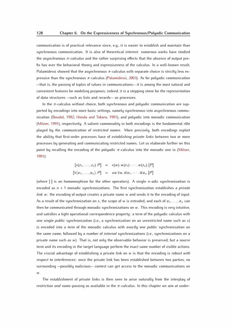
128 Chapter 6. On the Expressiveness of Synchronous/Polyadic Communication
communication is of practical relevance since, e.g., it is easier to establish and maintain thansynchronous communication. It is also of theoretical interest: numerous works have studiedthe asynchronous π-calculus and the rather surprising effects that the absence of output pre-fix has over the behavioral theory and expressiveness of the calculus. In a well-known result,Palamidessi showed that the asynchronous π-calculus with separate choice is strictly less ex-pressive than the synchronous π-calculus (Palamidessi, 2003). As for polyadic communicationthat is, the passing of tuples of values in communications it is among the most natural andconvenient features for modeling purposes; indeed, it is a stepping stone for the representationof data structures such as lists and records as processes.In the π-calculus without choice, both synchronous and polyadic communication are sup-ported by encodings into more basic settings, namely synchronous into asynchronous commu-nication (Boudol, 1992; Honda and Tokoro, 1991), and polyadic into monadic communication(Milner, 1991), respectively. A salient commonality in both encodings is the fundamental roleplayed by the communication of restricted names. More precisely, both encodings exploitthe ability that first-order processes have of establishing private links between two or moreprocesses by generating and communicating restricted names. Let us elaborate further on thispoint by recalling the encoding of the polyadic π-calculus into the monadic one in (Milner,1991):[[x(z1, . . . , zn).P]] = x(w).w(z1). · · · .w(zn). [[P]][[x〈a1, . . . , an〉.P]] = νw xw.wa1. · · · .wan. [[P]]
(where [[·]] is an homomorphism for the other operators). A single n-adic synchronization isencoded as n + 1 monadic synchronizations. The first synchronization establishes a privatelink w: the encoding of output creates a private name w and sends it to the encoding of input.As a result of the synchronization on x, the scope of w is extruded, and each of a1, . . . , an canthen be communicated through monadic synchronizations on w. This encoding is very intuitive,and satisfies a tight operational correspondence property: a term of the polyadic calculus withone single public synchronization (i.e., a synchronization on an unrestricted name such as x)is encoded into a term of the monadic calculus with exactly one public synchronization onthe same name, followed by a number of internal synchronizations (i.e., synchronizations on aprivate name such as w). That is, not only the observable behavior is preserved, but a sourceterm and its encoding in the target language perform the exact same number of visible actions.The crucial advantage of establishing a private link on w is that the encoding is robust withrespect to interferences: once the private link has been established between two parties, nosurrounding possibly malicious context can get access to the monadic communications onw. The establishment of private links is then seen to arise naturally from the interplay ofrestriction and name-passing as available in the π-calculus. In this chapter we aim at under-

6.1. Introduction 129
standing whether the settled situation in the first-order setting carries over to the higher-orderone. More precisely, we study the extent to which private links can be established in the con-text of HOCORE, a higher-order process calculus without name passing. This appears as aparticularly intriguing problem: in spite of its minimality, HOCORE is very expressive: not onlyit is Turing complete but also several modelling idioms (disjoint choice, input-guarded repli-cation, lists) are expressible in it as derived constructs. Hence, the answer to this question isfar from obvious.Here we shall consider two extensions of HOCORE. The first onedenoted AHOextendsHOCORE with restriction and polyadic communication; the second extensiondenoted SHOextends AHO with output prefixes, so as to represent synchronous process passing. Sinceboth calculi consider polyadic communication, AHO and SHO actually represent two familiesof higher-order process calculi: given n ≥ 0, we use SHOn (resp. AHOn) to denote thesynchronous (resp. asynchronous) higher-order process calculus with n-adic communication.It is useful to comment on the consequences of considering restricted names in higher-order process calculi without name-passing. The most notable one is the partial effect thatscope extrusions have. Let us explain what we mean by this. In a process-passing setting,received processes can only be executed, forwarded, or discarded. Hence, an input contextcannot gain access to the (private) names of those processes it receives; to the context receivedprocesses are much like a “black box”. Although higher-order communications might lead toscope extrusion of the private names contained in the transmitted processes, such extrusionsare vacuous: without name-passing, a receiving context can only use the names contained ina process in a restricted way, namely the way decreed by the sender of the process.1 Thesharing of (private) names one obtains from using process-passing only is then incomplete:names can be sent as part of processes but they cannot be freely used by a recipient.With the above discussion in mind, we begin by investigating the relationship betweensynchrony and asynchrony in process-passing calculi. Our first main result is an encoding ofSHO into AHO. Intuitively, a synchronous output is encoded by an asynchronous output thatcommunicates both the communication object and the continuation. This encodability resultis significant: it reveals that the absence of name passing does not necessarily imply thatencodings that rely on name-passing and private links are not expressible with process-passingonly. In fact, the encoding bears witness to the expressive power intrinsic to (asynchronous)process-passing.Based on this positive result, we move to examine the situation for polyadic communicationin process-passing calculi. We consider variants of SHO with different arity in communications,and study their relative expressive power. Interestingly, we determine that it is indeed the case1In this discussion we understand process-passing that does not consider abstraction-passing, i.e. the communica-tion of functions from processes to processes. As we shall see, the situation is rather different with abstraction-passing.
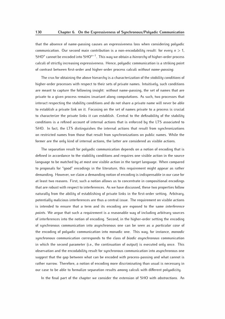
130 Chapter 6. On the Expressiveness of Synchronous/Polyadic Communication
that the absence of name-passing causes an expressiveness loss when considering polyadiccommunication. Our second main contribution is a non-encodability result: for every n > 1,SHOn cannot be encoded into SHOn−1. This way we obtain a hierarchy of higher-order processcalculi of strictly increasing expressiveness. Hence, polyadic communication is a striking pointof contrast between first-order and higher-order process calculi without name-passing.The crux for obtaining the above hierarchy is a characterization of the stability conditions ofhigher-order processes with respect to their sets of private names. Intuitively, such conditionsare meant to capture the following insight: without name-passing, the set of names that areprivate to a given process remains invariant along computations. As such, two processes thatinteract respecting the stability conditions and do not share a private name will never be ableto establish a private link on it. Focusing on the set of names private to a process is crucialto characterize the private links it can establish. Central to the definability of the stabilityconditions is a refined account of internal actions that is enforced by the LTS associated toSHO. In fact, the LTS distinguishes the internal actions that result from synchronizationson restricted names from those that result from synchronizations on public names. While theformer are the only kind of internal actions, the latter are considered as visible actions.The separation result for polyadic communication depends on a notion of encoding that isdefined in accordance to the stability conditions and requires one visible action in the sourcelanguage to be matched by at most one visible action in the target language. When comparedto proposals for “good” encodings in the literature, this requirement might appear as ratherdemanding. However, we claim a demanding notion of encoding is indispensable in our case forat least two reasons. First, such a notion allows us to concentrate in compositional encodingsthat are robust with respect to interferences. As we have discussed, these two properties follownaturally from the ability of establishing of private links in the first-order setting. Arbitrary,potentially malicious interferences are thus a central issue. The requirement on visible actionsis intended to ensure that a term and its encoding are exposed to the same interferencepoints. We argue that such a requirement is a reasonable way of including arbitrary sourcesof interferences into the notion of encoding. Second, in the higher-order setting the encodingof synchronous communication into asynchronous one can be seen as a particular case ofthe encoding of polyadic communication into monadic one. This way, for instance, monadicsynchronous communication corresponds to the class of biadic asynchronous communicationin which the second parameter (i.e., the continuation of output) is executed only once. Thisobservation and the encodability result for synchronous communication into asynchronous onesuggest that the gap between what can be encoded with process-passing and what cannot israther narrow. Therefore, a notion of encoding more discriminating than usual is necessary inour case to be able to formalize separation results among calculi with different polyadicity.In the final part of the chapter we consider the extension of SHO with abstractions. An

6.1. Introduction 131
abstraction is an expression of the form (x)Pit is a parameterized process. An abstractionhas a functional type. Applying an abstraction (x)P of type T → ♦ (where ♦ is the type ofall processes) to an argument W of type T yields the process P{W/x}. The argument Wcan itself be an abstraction; therefore the order of an abstraction, that is, the level of arrownesting in its type, can be arbitrarily high. The order can also be ω, if there are recursivetypes. We consider SHOna, the extension of SHOn with abstractions of order one (i.e., functionsfrom processes to processes). Our last main result shows that abstraction passing providesSHO with the ability of establishing of private links. Indeed, we show that SHOn can beencoded into SHO1a. This can be used to demonstrate that there is no encoding of SHOna intoSHOn. This result thus provides further evidence on the relationship between the ability ofestablishing private links and absolute expressiveness.Related Work. While a number of works address the relationship between synchronous andasynchronous communication in first-order calculi (see, e.g., (Palamidessi, 2003; Cacciagranoet al., 2007; Beauxis et al., 2008)), we are not aware of analogous studies for higher-orderprocess calculi. A similar situation occurs for the study of polyadic communication; in the first-order setting the interest has been in characterizing fully-abstract translations of polyadiccommunication into monadic one (see, e.g., (Quaglia and Walker, 2005; Yoshida, 1996)), butthe case of polyadicity in higher-order communication has not been addressed.The most related work is by Sangiorgi (1996b). There, the expressiveness of the π-calculuswith respect to higher-order π is studied by identifying hierarchies of fragments of first-orderand higher-order calculi with increasingly expressive power. The first-order hierarchy is basedon fragment of the π-calculus in which mobility is internal, i.e., where outputs are only onprivate names no free outputs are allowed. This hierarchy is denoted as πIn, where the ndenotes the degree of mobility allowed; this is formalized by means of dependency chainsin name creation. In this hierarchy, e.g., πI1 does not allow mobility and corresponds to thecore of CCS, and πIn will allow dependency chains of length at most n. The hierarchy inthe higher-order case follows a similar rationale, and is based on the strictly higher-orderπ-calculus, i.e., a higher-order calculus without name-passing features. Also in this hierarchy,the less expressive language (denoted HOπ1) corresponds to the core of CCS. Sangiorgi showsthat πIn and HOπn have the same expressiveness, by exhibiting fully-abstract encodings. Incontrast to (Sangiorgi, 1996b), the hierarchy of higher-order process calculi we consider hereis not given by the degree of mobility allowed, but by the size of the tuples that can be passedaround in polyadic communications.The distinction between internal and public synchronizations here proposed for our notionof encoding has been used and/or proposed in other contexts. In (Lanese, 2007) labels ofinternal actions are annotated with the name on which synchronization occurs so as to definelocated semantics which are then used to study concurrent semantics for the π-calculus using

132 Chapter 6. On the Expressiveness of Synchronous/Polyadic Communication
standard labeled transition systems. In the higher-order setting (Amadio, 1993) obtains afinitely-branching bisimilarity for CHOCS by means of a reduction into bisimulation for avariant of the π-calculus. In such a variant, processes are only allowed to exchange names ofactivation channels (i.e. the channels that trigger a copy of a process in the representation ofhigher-order communication with first-order one). The desired finitely-branching bisimilarityis obtained by relying on a labeled transition system in which synchronizations on activationchannels are distinguished.6.2 The Calculi
6.2.1 A Higher-Order Process Calculus with Restriction and Polyadic Com-munication
Here we define AHO, the extension of HOCORE with a restriction operator and polyadic com-munication. As such, it is asynchronous and does not feature name-passing.Definition 6.1. The language of AHO processes is given by the following syntax:
P,Q, . . . ::= a(x).P | a〈Q〉 | P1 ‖ P2 | νr P | x | 0
where x, y range over process variables, and a, b, r, s denote names.Assuming standard notation and properties for tuples of syntactic elements, polyadicityin process passing is interpreted as expected: an output message a〈Q〉 sends the tuple ofprocesses Q on name a; an input prefixed process a(x).P can receive a tuple Q on name (orchannel) a and continue as P{Q/x}. In both cases, a is said to be the subject of the action.We sometimes write | x | for the length of tuple x; the length of the tuples that are passedaround determines the actual arity in polyadic communication. In interactions, we assumeinputs and outputs agree on their arity; we shall rely on notions of types and well-typedprocesses as in (Sangiorgi, 1996b). Parallel composition allows processes to interact, andνr P makes r private (or restricted) to the process P. Notions of bound and free names andvariables (bn(·), fn(·), bv(·), and fv(·), resp.) are defined in the usual way: an input a(x).Pbinds the free occurrences of variables in x in P; similarly, νr P binds the free occurrences ofname r in P. We abbreviate a(x).P as a.P when none of the variables in x is in fv(P), anda〈0〉 as a. We use notation ∏k P to represent k copies of process P in parallel.
Definition 6.2. The structural congruence relation for AHO processes is the smallest congru-ence generated by the following laws: P ‖ 0 ≡ P, P1 ‖ P2 ≡ P2 ‖ P1, P1 ‖ (P2 ‖ P3) ≡(P1 ‖ P2) ‖ P3, νa νbP ≡ νb νaP, νa 0 ≡ 0, νa (P1 ‖ P2) ≡ νaP1 ‖ P2 if a 6∈ fn(P2).

6.2. The Calculi 133
INP a(x).P a(x)−−→ P OUT a〈Q〉 a〈Q〉−−−→ 0
ACT1 P1 α−→ P ′1 bv(α) ∩ fv(P2) = ∅P1 ‖ P2 α−→ P ′1 ‖ P2TAU1 P1 (νy)a〈〈P〉〉−−−−−−→ P ′1 P2 a(x)−−→ P ′2 y ∩ fn(P2) = ∅P1 ‖ P2 τ−−→ νy (P ′1 ‖ P ′2{P/x})
RES P α−→ P ′ r 6∈ n(α)νr P α−→ νr P ′OPEN P (νy)a〈〈P ′′〉〉−−−−−−→ P ′ x 6= a, x ∈ fn(P ′′)− yνx P (νxy)a〈〈P ′′〉〉−−−−−−−→ P ′
Figure 6.1: The LTS of AHO. We have omitted rules ACT2 and TAU2, the symmetric counter-parts of rules ACT1 and TAU1.The semantics for AHO is given in terms of the LTS given in Figure 6.1. There are threekinds of transitions: internal transitions P τ−−→ P ′, input transitions P a(x)−−→ P ′, and outputtransitions P (νy)a〈〈Q〉〉−−−−−−→ P ′ (with extrusion of the tuple of names y), which have the expectedmeaning. We use α to range over actions. The subject of action α , denoted as sub(α), isdefined as sub(a(x)) = a, sub(a〈〈Q〉〉) = a, and is undefined otherwise. Notions of boundand free names and variables extend to actions as expected. We sometimes use ~α to denote asequence of actions α1, . . . , αn. Weak transitions are defined in the usual way. We write =⇒for the reflexive, transitive closure of τ−−→. Given an action α , notation α=⇒ stands for =⇒ α−→=⇒.Given a sequence ~α = α1, . . . , αn, we define ~α=⇒ as α1=⇒ · · · αn=⇒.
Convention 6.1. In what follows we shall say that, for some n > 0, AHOn corresponds tothe higher-order process calculus obtained from the syntax given in Definition 6.1 in whichpolyadic communication has arity n.The following definition is standard.
Definition 6.3 (Strong and Weak Barbs). Given a process P and a name a, we write• P ↓a a strong input barb if P can perform an input action with subject a;• P ↓a a strong output barb if P can perform an output action with subject a.
Given µ ∈ {a, a}, we define a weak barb P ⇓µ if, for some P ′, P =⇒ P ′ ↓µ .
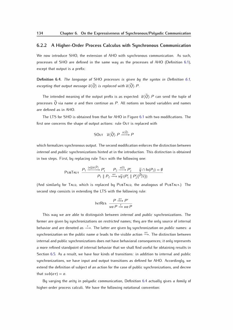
134 Chapter 6. On the Expressiveness of Synchronous/Polyadic Communication
6.2.2 A Higher-Order Process Calculus with Synchronous Communication
We now introduce SHO, the extension of AHO with synchronous communication. As such,processes of SHO are defined in the same way as the processes of AHO (Definition 6.1),except that output is a prefix:Definition 6.4. The language of SHO processes is given by the syntax in Definition 6.1,excepting that output message a〈Q〉 is replaced with a〈Q〉.P.
The intended meaning of the output prefix is as expected: a〈Q〉.P can send the tuple ofprocesses Q via name a and then continue as P. All notions on bound variables and namesare defined as in AHO.The LTS for SHO is obtained from that for AHO in Figure 6.1 with two modifications. Thefirst one concerns the shape of output actions: rule OUT is replaced withSOUT a〈Q〉.P a〈Q〉−−−→ P
which formalizes synchronous output. The second modification enforces the distinction betweeninternal and public synchronizations hinted at in the introduction. This distinction is obtainedin two steps. First, by replacing rule TAU1 with the following one:PUBTAU1 P1 (νy)a〈P〉−−−−−→ P ′1 P2 a(x)−−→ P ′2 y ∩ fn(P2) = ∅P1 ‖ P2 aτ−−→ νy (P ′1 ‖ P ′2{P/x})(And similarly for TAU2, which is replaced by PUBTAU2, the analogous of PUBTAU1.) Thesecond step consists in extending the LTS with the following rule:
INTRES P aτ−−→ P ′νaP τ−→ νaPThis way we are able to distinguish between internal and public synchronizations. Theformer are given by synchronizations on restricted names; they are the only source of internalbehavior and are denoted as τ−−→. The latter are given by synchronization on public names: asynchronization on the public name a leads to the visible action aτ−→. The distinction betweeninternal and public synchronizations does not have behavioral consequences; it only representsa more refined standpoint of internal behavior that we shall find useful for obtaining results inSection 6.5. As a result, we have four kinds of transitions: in addition to internal and publicsynchronizations, we have input and output transitions as defined for AHO. Accordingly, weextend the definition of subject of an action for the case of public synchronizations, and decreethat sub(aτ) = a.By varying the arity in polyadic communication, Definition 6.4 actually gives a family ofhigher-order process calculi. We have the following notational convention:
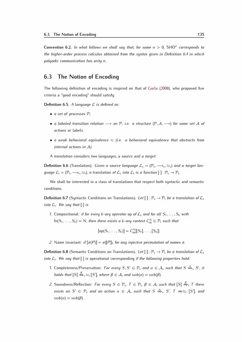
6.3. The Notion of Encoding 135
Convention 6.2. In what follows we shall say that, for some n > 0, SHOn corresponds tothe higher-order process calculus obtained from the syntax given in Definition 6.4 in whichpolyadic communication has arity n.6.3 The Notion of Encoding
The following definition of encoding is inspired on that of Gorla (2008), who proposed fivecriteria a “good encoding” should satisfy.Definition 6.5. A language L is defined as:
• a set of processes P;• a labeled transition relation −→ on P, i.e. a structure (P,A,−→) for some set A ofactions or labels.• a weak behavioral equivalence ≈ (i.e. a behavioral equivalence that abstracts frominternal actions in A).A translation considers two languages, a source and a target:
Definition 6.6 (Translation). Given a source language Ls = (Ps,−→s,≈s) and a target lan-guage Lt = (Pt,−→t,≈t), a translation of Ls into Lt is a function [[·]] : Ps → Pt.We shall be interested in a class of translations that respect both syntactic and semanticconditions.
Definition 6.7 (Syntactic Conditions on Translations). Let [[·]] : Ps → Pt be a translation of Lsinto Lt. We say that [[·]] is1. Compositional: if for every k-ary operator op of Ls and for all S1, . . . , Sk withfn(S1, . . . , Sk ) = N, then there exists a k-ary context CNop ∈ Pt such that
[[op(S1, . . . , Sk )]] = CNop[[[S1]], . . . , [[Sk ]]].2. Name invariant: if [[σ (P)]] = σ ([[P]]), for any injective permutation of names σ .
Definition 6.8 (Semantic Conditions on Translations). Let [[·]] : Ps → Pt be a translation of Lsinto Lt. We say that [[·]] is operational corresponding if the following properties hold:1. Completeness/Preservation: For every S, S′ ∈ Ps and α ∈ As such that S α=⇒s S′, itholds that [[S]] β=⇒t≈t [[S′]], where β ∈ At and sub(α) = sub(β).2. Soundness/Reflection: For every S ∈ Ps, T ∈ Pt, β ∈ At such that [[S]] β=⇒t T thereexists an S′ ∈ Ps and an action α ∈ As such that S α=⇒s S′, T =⇒≈t [[S′]], andsub(α) = sub(β).

136 Chapter 6. On the Expressiveness of Synchronous/Polyadic Communication
Furthermore, we shall require adequacy: if P ≈s Q then [[P]] ≈t [[Q]].Notice that adequacy is necessary because we make no assumptions on the nature of ≈sand ≈t.
Definition 6.9. We call encoding any translation that satisfies both the syntactic conditionsin Definition 6.7 and the semantic conditions in Definition 6.8.Remark 6.1. Notice that our definition of encoding intends to capture the fact that an actionin the source language might be not matched by the exact same action in the target language.Some Properties of Encodings.
Proposition 6.1. Let a be a name. If a ∈ fn(P) then also a ∈ fn([[P]]).Proof. By contradiction. Take two distinct names a and b. Suppose a is free in P. Clearly,we have that P{b/a} 6= P (∗)Suppose, for the sake of contradiction, that a is not free in [[P]]. Under that assumption, onehas that [[P]]{b/a} = [[P]] as substituting a non-free name with another name is a vacuousoperation. Notice that by name invariance one has [[P]]{b/a} = [[P{b/a}]]. Now, considering (∗)above, one has the [[P]]{b/a} 6= [[P{b/a}]], a contradiction.Proposition 6.2. Let [[·]] be an encoding of Ls into Lt. Then [[·]] satisfies:
1. Barb preservation: for every S ∈ Ps it holds that S ⇓a (resp. S ⇓a) if and only if [[S]] ⇓a(resp. [[S]] ⇓a).Proof. It follows from operational correspondence in the definition of encoding (Definition6.9)Proposition 6.3 (Composability of Encodings). If C[[·]] is an encoding of L1 into L2, and D [[·]] isan encoding of L2 into L3 then their composition (D · C)[[·]] is an encoding of L1 into L3.Proof. From the definition of encoding (Definition 6.9). The syntactic conditions (composition-ality, name invariance) are easily seen to hold for (D ·C)[[·]]; the semantic conditions (operationalcorrespondence, adequacy) rely on the fact that ≈1,≈2, and ≈3 are equivalences and hencetransitive. Note that adequacy is crucial to show the composability for operational correspon-dence.

6.4. An Encodability Result for Synchronous Communication 137
6.4 An Encodability Result for Synchronous Communication
We begin by studying the relationship between synchronous and asynchronous communication.The main result of this section is an encoding of SHOn into AHOn.A naive encoding would simply consist in sending both the communication object andthe continuation of the output action in a single synchronization. The continuation is sentexplicitly as a parameter, and so a synchronous calculus with polyadicity n would have to beencoded into an asynchronous calculus with polyadicity n+ 1. To illustrate this, consider thenaive encoding of SHO1 into AHO2:[[a〈P〉.S]] = a〈[[P]], [[S]]〉[[a(x).R ]] = a(x, y). (y ‖ [[R ]])
where [[·]] is an homomorphism for the other operators in SHO1. This encoding allows toappreciate how in the higher-order setting the synchronous/asynchronous distinction can beconsidered as a particular case of the polyadic/monadic distinction. Notice that the fact thatthe continuation is supposed to be executed only once is crucial for the simplicity of theencoding.Interestingly, we notice that asynchronous process-passing is expressive enough so as toencode synchronous communication of the same arity. Intuitively, the idea is to send a singleprocess consisting of a guarded choice between a communication object and the continuationof the synchronous output. For the monadic case the encoding is as follows:[[a〈P〉.S]] = νk, l (a〈k . ([[P]] ‖ k) + l. ([[S]] ‖ k)〉 ‖ l)[[a(x).R ]] = a(x). (x ‖ [[R ]])
where “+” stands for the encoding of disjoint choice in HOCORE, presented in Section 3.2;k, l are two names not in fn(P,S); and [[·]] is an homomorphism for the other operators in SHO1.The synchronous output action is thus encoded by sending a guarded, disjoint choicebetween the encoding of the communication object and the encoding of the continuation ofthe output. The encoding exploits the fact that the continuation should be executed exactlyonce, while the communication object can be executed zero or more times. Notice that there isonly one copy of the trigger that executes the encoding of the continuation (denoted l in theencoding above), which guarantees that it is executed exactly once. This can only occur afterthat the synchronization has taken place, thus ensuring a correct encoding of synchronouscommunication. Notice that l releases both the encoding of the continuation and a trigger forexecuting the encoding of the communication object (denoted k); such an execution will onlyoccur when the choice sent by the encoding of output appears at the top level. This way, it

138 Chapter 6. On the Expressiveness of Synchronous/Polyadic Communication
is easy to see that a trigger k is always available. This idea can be generalized to encodesynchronous calculi of arbitrary polyadicity as follows:Definition 6.10 (Synchronous into Asynchronous). For some n > 0, the encoding of SHOninto AHOn is defined as follows:
[[a〈P1, . . . , Pn〉.S]] = νk, l (a〈[[P1]], . . . , [[Pn−1]], Tk,l[ [[Pn]], [[S]] ]〉 ‖ l)[[a(x1, . . . , xn).R ]] = a(x1, . . . , xn). (xn ‖ [[R ]])with Tk,l[M1,M2] = k . (M1 ‖ k) + l. (M2 ‖ k)where {k, l} ∩ fn(P1, . . . , Pn, S) = ∅, and [[·]] is an homomorphism for the other operators inSHOn.Proposition 6.4 (Correctness of the Encoding). The translation in Definition 6.10 is an encod-ing in the sense of Definition 6.9.Proof (Sketch). It is immediate to observe that the encoding respects syntactic conditions asin Definition 6.7. To show operational correspondence as in Definition 6.8, one defines acharacterization of the “garbage” that the process leaves along reductions. Such garbage isessentially determined by occurrences of the trigger that activates a copy to (the encodingof) the last parameter of the polyadic communication (denoted k in Definition 6.10). Suchoccurrences remain while the summation that the encoding sends is not at the top-level; sometriggers might remain even if all summations have been consumed. Crucially, since suchtriggers are on restricted names, they are harmless for the rest of the process, and so theencoding is correct up to these extra triggers.
The encoding is significant as it provides compelling evidence on the expressive power that(asynchronous) process-passing has for representing protocols that rely on establishment ofprivate links in the first-order setting. Not only the encoding bears witness of the fact thatsuch protocols can indeed be encoded into calculi with process-passing only; the observationthat the encoding of synchronous into asynchronous communication is a particular case of thatof polyadic into monadic communication leaves open the possibility that, following a similarstructure, an encoding of polyadic communication (as the proposed by Milner) might exist forthe case of process-passing. In the next section we prove that this is not the case.6.5 Separation Results for Polyadic Communication
In this section we present the separability results for SHO. First, Then, in Section 6.5.1, weintroduce the notion of distinguished forms, which allow us to capture a number of stability

6.5. Separation Results for Polyadic Communication 139
conditions of processes with respect to their sets of private names. in Section 6.5.2 we presentthe hierarchy of SHO calculi based on polyadic communication.6.5.1 Distinguished Forms
Here we define a number of distinguished forms for SHO processes. They are intended tocapture the structure of processes along communications, focusing on the private names sharedamong the participants.6.5.1.1 Definition
The definition of distinguished forms exploits contexts, that is, processes with a hole. Weshall consider multi-hole contexts, that is, contexts with more than one hole. More precisely,a multi-hole context is n-ary if at most n different holes [·]1, . . . , [·]n, occur in it. (A processis a 0-ary multi-hole context.) We will assume that any hole [·]i can occur more than oncein the context expression. Notions of free and bound names for contexts are as expected anddenoted bn(·) and fn(·), respectively.Definition 6.11. Syntax of (guarded, multihole) contexts:
C, C ′, . . . ::= a(x).D | a〈D〉.DD,D′, . . . ::= [·] | P | C | D ‖ D | νr DRemark 6.2. We are always working with non-binding contexts, i.e., contexts that do notcapture the free variables of the processes that fill their holes.
Below we define disjoint forms, the main distinguished form we shall use in the chapter.Definition 6.12 (Disjoint Form). Let T ≡ νn(P ‖ C [R ]) be a SHOm process where
1. n is a set of names such that n ⊆ fn(P, R) and n ∩ fn(C ) = ∅;2. C is a k-ary (guarded, multihole) context;3. R contains k closed processes.
We then say that T is in k-adic disjoint form with respect to n, R , and P.The above definition decrees an arbitrary arity for the context. We shall sometimes saythat processes in such a form are in n-adic disjoint form, or NDF. By restricting the arity ofthe context, this general definition can be instantiated:
Definition 6.13 (Monadic Disjoint Form, MDF). Suppose a process T that is in disjoint formwith respect to some n, R , and P. If | R |= 1 then T is said to be in monadic disjoint form (orMDF) with respect to n, R , and P.

140 Chapter 6. On the Expressiveness of Synchronous/Polyadic Communication
Recall that even if MDFs have monadic contexts, the content of the hole (i.e. the singleprocess R) can appear more than once in the process. It could even be the case the contentdoes not appear at all. This is a special case of MDF, as we define below:Definition 6.14 (Zero-adic Disjoint Form, ZDF). Let T ≡ νn (P ‖ C [R ]) be in MDF withrespect to n, R , and P. If C [R ] 6= ∅ and R = 0 then T is said to be in zero-adic disjointform (ZDF) with respect to n and P. Moreover, T can be rewritten as T ≡ νn1P ‖ νn2Q, forsome Q ≡ C [0] and for some disjoint sets of names n1 and n2 such that both n = n1 ∪ n2 andn1 ∩ n2 = ∅ hold.
The following property will be useful in proofs.Proposition 6.5 (Encodings preserve ZDFs). Let [[·]] be an encoding as in Definition 6.9. If Tis in ZDF with respect to some n and P then [[T ]] is in ZDF with respect to n and [[P]].Proof. We know that, for some Q and m, T ≡ νn P ‖ νmQ is in ZDF with respect to n andP, and that n ∩ m = ∅. By compositionality (Definition 6.7(1)) we have that, for some contextC , [[T ]] = C [[[νn P]], [[νmQ]]]. The sensible issue here is to ensure that [[νn P]] and [[νmQ]] do notshare private names because of the enclosing context C . There are two cases: the first oneis that a name that is free in νn P but private to νmQ becomes private in both [[νn P]] and[[νmQ]] (and the symmetric case); the second case is that a name that is free in both νn Pand νmQ becomes private in both [[νn P]] and [[νmQ]]. Proposition 6.1 ensures that none ofthese cases is possible; for every name a and process R , such a proposition guarantees thatif a ∈ fn(R) then also a ∈ fn([[R ]]). As a consequence, even if the context C could involverestrictions enclosing both [[νn P]] and [[νmQ]], such restriction will not bind names in them.Notice that C [[[νn P]], [[νmQ]]] can be rewritten as [[T ]] ≡ νa([[νn P]] ‖ [[νmQ]] ‖ S), for someprocess S. Because of the discussion before, names in a do not bind names in [[P]] nor in [[Q]].Hence, [[T ]] is in ZDF with respect to [[P]] and n, as desired.
6.5.1.2 Properties of Disjoint Forms I: Stability Conditions
We are interested in characterizing the transitions that preserve disjoint forms. We focus oninternal and output actions. In what follows we discuss properties that apply to arbitraryNDFs; for the sake of readability, however, in proofs we sometimes restrict ourselves to thecase of MDFs, since cases for other disjoint forms are analogous and only differ in notationalburden.The following proposition formalizes that, up-to structural congruence, derivatives of NDFsthat have unguarded occurrences of some Ri can be brought back into an NDF by “pushing”such occurrences into the side of P of the NDF.
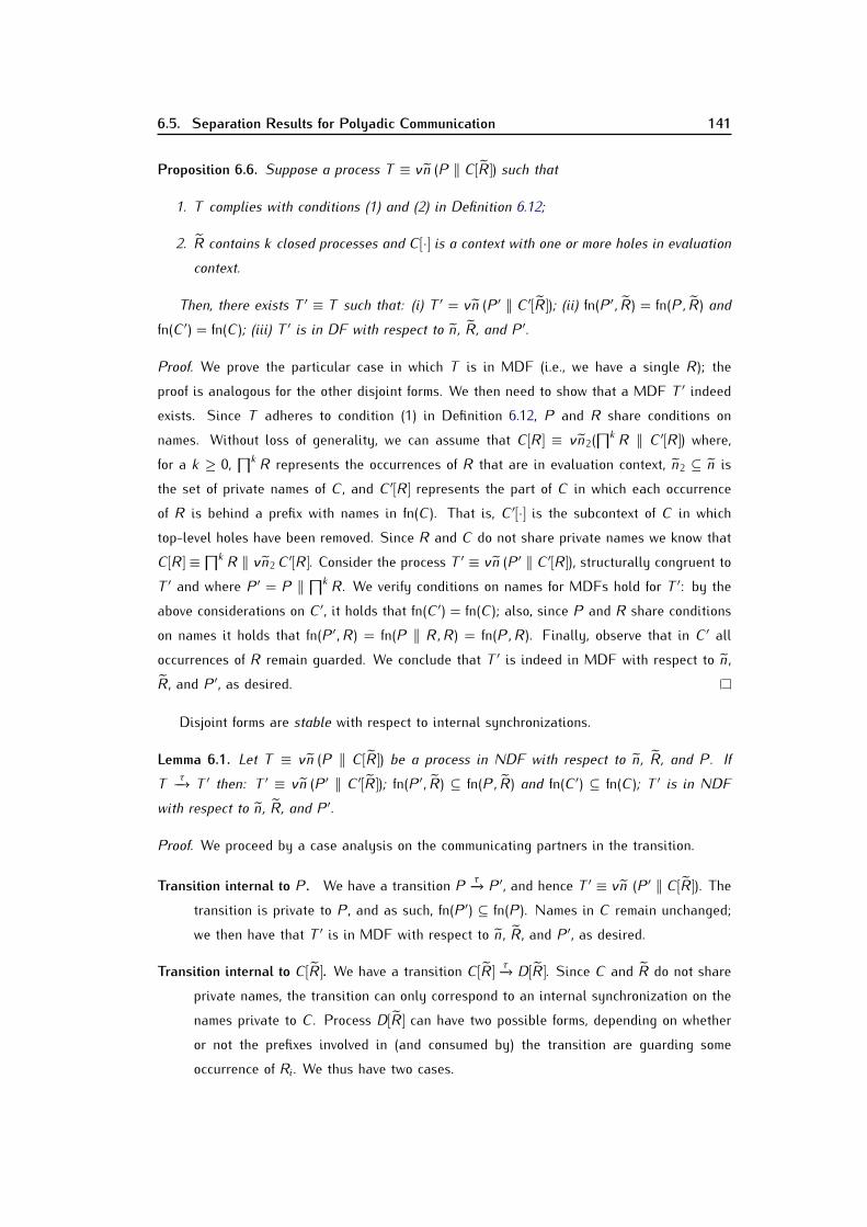
6.5. Separation Results for Polyadic Communication 141
Proposition 6.6. Suppose a process T ≡ νn (P ‖ C [R ]) such that1. T complies with conditions (1) and (2) in Definition 6.12;2. R contains k closed processes and C [·] is a context with one or more holes in evaluationcontext.Then, there exists T ′ ≡ T such that: (i) T ′ = νn (P ′ ‖ C ′[R ]); (ii) fn(P ′, R) = fn(P, R) andfn(C ′) = fn(C ); (iii) T ′ is in DF with respect to n, R , and P ′.
Proof. We prove the particular case in which T is in MDF (i.e., we have a single R); theproof is analogous for the other disjoint forms. We then need to show that a MDF T ′ indeedexists. Since T adheres to condition (1) in Definition 6.12, P and R share conditions onnames. Without loss of generality, we can assume that C [R ] ≡ νn2(∏k R ‖ C ′[R ]) where,for a k ≥ 0, ∏k R represents the occurrences of R that are in evaluation context, n2 ⊆ n isthe set of private names of C , and C ′[R ] represents the part of C in which each occurrenceof R is behind a prefix with names in fn(C ). That is, C ′[·] is the subcontext of C in whichtop-level holes have been removed. Since R and C do not share private names we know thatC [R ] ≡∏k R ‖ νn2 C ′[R ]. Consider the process T ′ ≡ νn (P ′ ‖ C ′[R ]), structurally congruent toT ′ and where P ′ = P ‖ ∏k R . We verify conditions on names for MDFs hold for T ′: by theabove considerations on C ′, it holds that fn(C ′) = fn(C ); also, since P and R share conditionson names it holds that fn(P ′, R) = fn(P ‖ R,R) = fn(P,R). Finally, observe that in C ′ alloccurrences of R remain guarded. We conclude that T ′ is indeed in MDF with respect to n,R , and P ′, as desired.Disjoint forms are stable with respect to internal synchronizations.
Lemma 6.1. Let T ≡ νn (P ‖ C [R ]) be a process in NDF with respect to n, R , and P. IfT τ−→ T ′ then: T ′ ≡ νn (P ′ ‖ C ′[R ]); fn(P ′, R) ⊆ fn(P, R) and fn(C ′) ⊆ fn(C ); T ′ is in NDFwith respect to n, R , and P ′.Proof. We proceed by a case analysis on the communicating partners in the transition.Transition internal to P. We have a transition P τ−→ P ′, and hence T ′ ≡ νn (P ′ ‖ C [R ]). Thetransition is private to P, and as such, fn(P ′) ⊆ fn(P). Names in C remain unchanged;we then have that T ′ is in MDF with respect to n, R , and P ′, as desired.Transition internal to C [R ]. We have a transition C [R ] τ−→ D[R ]. Since C and R do not shareprivate names, the transition can only correspond to an internal synchronization on thenames private to C . Process D[R ] can have two possible forms, depending on whetheror not the prefixes involved in (and consumed by) the transition are guarding someoccurrence of Ri. We thus have two cases.

142 Chapter 6. On the Expressiveness of Synchronous/Polyadic Communication
1. In the case D[R ] has no unguarded occurrences of R (i.e. there are no holes at thetop level of the context), we have D ≡ C ′[R ], for a context C ′ that is exactly as Cexcept from two prefixes. The transition concerns only names private to C ; hence,fn(C ′) ⊆ fn(C ) and the other conditions on names are not affected. We then havethat T ′ = νn (P ‖ C ′[R ]) is in NDF with respect to n, R , and P, as desired.2. In the case occurrences of some Ri end up unguarded after the transition, with theaid of Proposition 6.6 we infer that T ′ is structurally congruent to a MDF withrespect to n, R , and P, and we are done.
Transition internal to some Ri. This is not possible as by definition of disjoint form, everyoccurrence of R in C [R ] is underneath a prefix.Communication between P and C [R ]. This is not possible since by definition of disjoint form,P and C do not share private names. No Ri can evolve, thus there cannot be a commu-nication between P and any Ri.
Corollary 6.1. Let T be a process in ZDF with respect to some n and P. If T τ−→ T ′, then T ′is in ZDF with respect to n and P too.The lemma below asserts that disjoint forms are stable also under output actions that donot involve extrusion of names. To see this, consider a MDF T : the only risk for it after anoutput action is that the R in C [R ] could be communicated, therefore “downgrading” the MDFinto a ZDF. Since, as we have seen, ZDFs are a special case of MDFs, this is not a problemand MDFs are preserved. Below we say a process P is contained in a process Q if and onlyif there exists a context C such that Q ≡ C [P].
Lemma 6.2. Let T ≡ νn (P ‖ C [R ]) be a process in NDF with respect to n, R , and P. IfT a〈Q〉−−−→ T ′ then: there exist P ′ and C ′ so that T ′ ≡ νn (P ′ ‖ C ′[R ]); both fn(P ′, R) ⊆ fn(P, R)and fn(C ′) ⊆ fn(C ) hold; T ′ is in MDF with respect to n, R , and P ′.Proof. By a case analysis on the source of the action. We prove the particular case in whichT is in MDF; the proof is analogous for the other disjoint forms.
• If P a〈Q〉−−−→ P ′ then T ′ ≡ νn (P ′ ‖ C [R ]). Since P ′ is contained in P, we have fn(P ′, R) ⊆fn(P,R). Conditions on names in fn(C ) are unchanged, and we have that T ′ is in MDFwith respect to n, R , and P ′, as desired.• If C [R ] a〈Q〉−−−→ D[R ] then we reason on k , the number of guarded occurrences of R in D[R ].The thesis is immediate for k > 0; if k = 0 then D[R ] is actually in ZDF with respect ton and P; by recalling that a ZDF is a special case of MDF we are done.
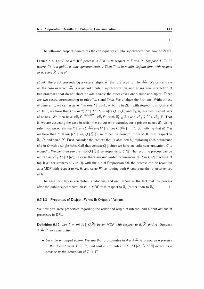
6.5. Separation Results for Polyadic Communication 143
The following property formalizes the consequences public synchronizations have on ZDFs.Lemma 6.3. Let T be a SHOn process in ZDF with respect to n and P. Suppose T aτ−→ T ′where aτ−→ is a public n-adic synchronization. Then T ′ is in n-adic disjoint form with respectto n, some R , and P.Proof. The proof proceeds by a case analysis on the rule used to infer aτ−→. We concentrateon the case in which aτ−→ is a monadic public synchronization, and arises from interaction oftwo processes that do not share private names; the other cases are similar or simpler. Thereare two cases, corresponding to rules TAU1 and TAU2. We analyze the first one. Without lossof generality, we can assume T ≡ νn1P ‖ νn2Q, which is in ZDF with respect to n1 ∪ n2 andP. In T , we have that P = a〈R〉.P ′ ‖ P ′′, Q = a(x).Q′ ‖ Q′′, and n1, n2 are two disjoint setsof names. We then have νn1 P (νn′1)a〈R〉−−−−−→ νn1 P ′ (with n′1 ⊆ n1) and νn2Q a(x)−−→ νn2Q′. Thatis, we are assuming the case in which the output on a extrudes some private names n′1. Usingrule TAU1 we obtain νn1P ‖ νn2Q aτ−→ νn1 P ′ ‖ νn′1n2Q′{R/x} = T ′. By noticing that n′1 ⊆ nwe have that T ′ ≡ νn1 (P ′ ‖ νn2Q′{R/x}), so T ′ can be brought into a MDF with respect ton1, R , and some P ′. First, consider the context that is obtained by replacing each occurrenceof x in Q with a single hole. Call that context C [·]; since we have monadic communication, C ismonadic. We can then see that νn2Q′{R/x} corresponds to C [R ]. The resulting process can bewritten as νn1 (P ′ ‖ C [R ]); in case there are unguarded occurrences of R in C [R ] (because oftop-level occurrences of x in Q), with the aid of Proposition 6.6, the process can be rewrittenas a MDF with respect to n1, R , and some P ′′ containing both P ′ and a number of occurrencesof R .The case for TAU2 is completely analogous, and only differs in the fact that the processafter the public synchronization is in MDF with respect to n2 (rather than to n1).6.5.1.3 Properties of Disjoint Forms II: Origin of Actions
We now give some properties regarding the order and origin of internal and output actions ofprocesses in DFs.Definition 6.15. Let T = νn (A ‖ C [R ]) be an NDF with respect to n, R , and A. SupposeT α−→ T ′ for some action α .
• Let α be an output action. We say that α originates in A if A α−→ A′ occurs as a premisein the derivation of T α−→ T ′, and that α originates in C if C [R ] α−→ C ′[R ] occurs as apremise in the derivation of T α−→ T ′.
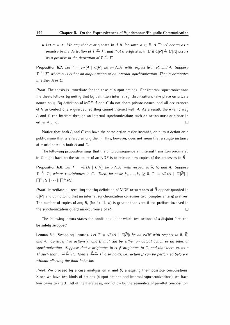
144 Chapter 6. On the Expressiveness of Synchronous/Polyadic Communication
• Let α = τ. We say that α originates in A if, for some a ∈ n, A aτ−→ A′ occurs as apremise in the derivation of T α−→ T ′, and that α originates in C if C [R ] τ−→ C ′[R ] occursas a premise in the derivation of T α−→ T ′.Proposition 6.7. Let T = νn (A ‖ C [R ]) be an NDF with respect to n, R , and A. SupposeT α−→ T ′, where α is either an output action or an internal synchronization. Then α originatesin either A or C .Proof. The thesis is immediate for the case of output actions. For internal synchronizationsthe thesis follows by noting that by definition internal synchronizations take place on privatenames only. By definition of MDF, A and C do not share private names, and all occurrencesof R in context C are guarded, so they cannot interact with A. As a result, there is no wayA and C can interact through an internal synchronization; such an action must originate ineither A or C .
Notice that both A and C can have the same action α (for instance, an output action on apublic name that is shared among them). This, however, does not mean that a single instanceof α originates in both A and C .The following proposition says that the only consequence an internal transition originatedin C might have on the structure of an NDF is to release new copies of the processes in R :Proposition 6.8. Let T = νn (A ‖ C [R ]) be a NDF with respect to n, R , and A. SupposeT τ−→ T ′, where τ originates in C . Then, for some k1, . . . , kn ≥ 0, T ′ ≡ νn (A ‖ C ′[R ] ‖∏k1 R1 ‖ · · · ‖∏kn Rn).Proof. Immediate by recalling that by definition of MDF occurrences of R appear guarded inC [R ], and by noticing that an internal synchronization consumes two (complementary) prefixes.The number of copies of any Ri (for i ∈ 1. .n) is greater than zero if the prefixes involved inthe synchronization guard an occurrence of Ri.
The following lemma states the conditions under which two actions of a disjoint form canbe safely swapped.Lemma 6.4 (Swapping Lemma). Let T = νn (A ‖ C [R ]) be an NDF with respect to n, R ,and A. Consider two actions α and β that can be either an output action or an internalsynchronization. Suppose that α originates in A, β originates in C , and that there exists aT ′ such that T α−→ β−→ T ′. Then T β−→ α−→ T ′ also holds, i.e., action β can be performed before αwithout affecting the final behavior.Proof. We proceed by a case analysis on α and β, analyzing their possible combinations.Since we have two kinds of actions (output actions and internal synchronizations), we havefour cases to check. All of them are easy, and follow by the semantics of parallel composition.

6.5. Separation Results for Polyadic Communication 145
Consider, for instance, in the case in which α = τ through a synchronization on private namea, and β = τ through a synchronization on private name a. Then, for some complementaryactions α0, α0 on (private) name a, and complementary actions β0, β0 on (private) name b, wehave thatT ≡ νn (α0.A1 ‖ α0.A2 ‖ A′ ‖ β0.C1[R ] ‖ β0.C2[R ] ‖ C ′[R ]) andT ′ ≡ νn (A1 ‖ A2 ‖ A′ ‖ C1[R ] ‖ C2[R ] ‖ C ′[R ])
By definition of internal synchronizations, a is a name private to A and b is a name private toC . Since by definition of MDF A and C do not share private names, then there is no possibilityfor interferences between the prefixes α0, α0, β0, and β0. Hence, it is safe to perform T β−→ α−→ T ′,and the thesis holds.Notice that the converse of the Swapping Lemma does not hold: since an action β origi-nated in C can enable an action α originated in A (e.g., an action enabled by an extra copyof R), these cannot be swapped. We now generalize the Swapping Lemma to a sequence ofinternal synchronizations and output actions.
Lemma 6.5 (Commuting Lemma). Let T = νn (A ‖ C [R ]) be a NDF with respect to n, R , andA. Suppose T ~α=⇒ T ′, where ~α is a sequence of output actions and internal synchronizationsonly. Let ~αC (resp. ~αA) be the sequence of actions that is exactly as ~α but in which actionsoriginated in A (resp. C ) or its derivatives are not included. Then, there exists a process T1such that1. T ~αC=⇒ T1 ~αA=⇒ T ′.2. T1 ≡ νn (A ‖∏m1 R1 ‖ · · · ‖∏mk Rn ‖ C ′[R ]), for some m1, . . . , mk ≥ 0.
Proof. We proceed by an induction on k , the number of actions originated in C that occurafter an action originated in A in the sequence ~α . The base case is when k = 0; that is, whenall the actions after T1 are originated in A, and we are done. The inductive step requires asecond induction on j , the number of actions originated in A which precede a single actionoriginated in C . This induction follows easily exploiting the Swapping Lemma (Lemma 6.4).The fact that, for each i ∈ 1. .n, T1 involves a number mi ≥ 0 of copies of Ri is an immediateconsequence of Proposition 6.8.6.5.2 A Hierarchy of Synchronous Higher-Order Process Calculi
We define an expressiveness hierarchy for the higher-order process calculi in the family givenby SHO. The hierarchy is defined in terms of the impossibility of encoding SHOn into SHOn−1,according to the definition given in Section 6.3. We begin by showing the impossibility resultthat sets the basic case of the hierarchy, namely that biadic process passing cannot be encoded

146 Chapter 6. On the Expressiveness of Synchronous/Polyadic Communication
into monadic process passing (Lemma 6.6). The proof exploits the notion of MDF and itsassociated stability properties. We then state the general result, i.e. the impossibility ofencoding SHOn+1 into SHOn (Lemma 6.7); this is done by generalizing the proof of Lemma6.6.Lemma 6.6. There is no encoding of SHO2 into SHO1.Proof. Assume, towards a contradiction, that an encoding [[·]] : SHO2 → SHO1 does indeedexist. In what follows, we use i, j to range over {1, 2}, assuming that i 6= j .Assume processes Si = mi ‖ mi. si and Sj = mj ‖ mj . sj . Consider the SHO2 processP = E (2) ‖ F (2), where E (2) and F (2) are defined as follows:
E (2) = νm1, m2 (a〈〈〉S1, S2〉. 0)F (2) = νb (a(x1, x2). (b〈〈〉b1. x1〉. 0 ‖ b〈〈〉b2. x2〉. 0 ‖ b(y1).b(y2).y1))where both b1, b2 6∈ fn(E (2)) (with b1 6= b2) and s1, s2 6∈ fn(F (2)) (with s1 6= s2) hold. Let usanalyze the behavior of P. We first have a public synchronization on a:
P aτ−→ νm1, m2, b (b〈〈〉b1.S1〉. 0 ‖ b〈〈〉b2.S2〉. 0 ‖ b(y1).b(y2).y1) = P0 .In P0 we have two private synchronizations on name b that implement an internal choice: bothprocesses b1.S1 and b2.S2 are consumed but only one of them will be executed. We then haveeither P0 τ−−→ τ−−→ b1.S1 = P1 or P0 τ−−→ τ−−→ b2.S2 = P ′1. Starting in P1 and P ′1 we have thefollowing sequences of actions:
P1 b1−→ P2 τ−−→ s1−→ 0P ′1 b2−→ P ′2 τ−−→ s2−→ 0 .In both cases, a private synchronization on mi precedes an output action on si. All the abovecan be summarized as follows:
P aτ−→ P0 τ−−→ τ−−→ P1 b1−→ P2 τ−−→ s1−→ 0 (6.1)P aτ−→ P0 τ−−→ τ−−→ P ′1 b2−→ P ′2 τ−−→ s2−→ 0 . (6.2)These sequences of actions might help to appreciate the effects of the internal choice on b,discussed above. Such a choice has direct influence on: (i) the output action on bi, (ii) theinternal synchronization on mi, and (iii) the output action on si. Notice that each of theseactions enables the following one, and that an output on bi precludes the possibility of actionson bj , mj , and sj .Consider now the behavior of [[P]] the encoding of P with the aid of (6.1) and (6.2) above.By definition of encoding (in particular, completeness) we have the following two, mutually

6.5. Separation Results for Polyadic Communication 147
exclusive, possibilities for behavior:[[P]] aτ=⇒≈ [[P0]] =⇒≈ [[P1]] b1=⇒≈ [[P2]] s1=⇒≈ 0 and (6.3)[[P]] aτ=⇒≈ [[P0]] =⇒≈ [[P ′1]] b2=⇒≈ [[P ′2]] s2=⇒≈ 0 . (6.4)
We notice that the first (weak) transition, namely[[P]] aτ=⇒≈ [[P0]] ,
is the same in both possibilities. Let us analyze it, by relying on Definition 6.3. For SHO1processes T , T ′, and T0, it holds
[[P]] =⇒ T aτ−→ T ′ =⇒ T0 ≈ [[P0]] . (6.5)We examine the distinguished forms in the processes in (6.5). We notice that P is in ZDFwith respect to {m1, m2, b} and E (2): m1, m2 do not appear in F (2), and b does not appear inE (2). From Proposition 6.5 we know that [[P]] is also in ZDF with respect to {m1, m2, b} and[[E (2)]]. Since DFs are preserved by internal actions (Corollary 6.1), we know that T is also aZDF with respect to {m1, m2, b} and A, the derivative of [[E (2)]]. In the general case, Lemma 6.3ensures that a public synchronization causes a ZDF to become a MDF. In this case, we havea communication from E (2) to F (2) which is mimicked by the encoding; we then have that T ′is in MDF with respect to {m1, m2}, some R 6= 0, and A′, the derivative of A after the publicsynchronization. Finally, since T ′ evolves into T0 by means of internal synchronizations only,by Lemma 6.1, we know that T0 is also in MDF with respect to {m1, m2}, R , and A0, thederivative of A′. Indeed, for some context C0 (with private name b), we have that
T0 = νm1, m2 (A0 ‖ C0[R ]) .Notice that (6.5) ensures that process T0 ≈ [[P0]]. Hence, by definition of ≈, T0 shouldbe able to match each action possible from [[P0]] by performing either the sequence of actionsgiven in (6.3) or the one in (6.4). We have just seen that T0 is in MDF with respect to{m1, m2}, R , and A0. Crucially, both (6.3) and (6.4) involve only internal synchronizations andoutput actions. Therefore, by Lemmas 6.1 and 6.2, every derivative of T0 intended to mimic thebehavior of [[P0]] (and its derivatives) is a process in MDF with respect to {m1, m2}, R , andsome Ai.We now use this information on the structure of the derivatives of T0 to analyze thebisimulation game for T0 ≈ [[P0]]. We use the observability predicates (barbs) as in Definition6.3. We know from (6.3) and (6.4) that [[P0]] evolves into either [[P1]] or [[P ′1]] after a weaktransition. The encoding preserves the mutually exclusive, internal choice that was discussedfor the source term P0; in the encoding such a choice is governed by the encoding of F (2).Also, as in the source term, the output barb on bi (resp. bj ) available in [[P1]] (resp. [[P ′1]]) is
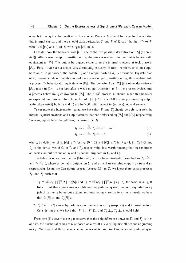
148 Chapter 6. On the Expressiveness of Synchronous/Polyadic Communication
enough to recognize the result of such a choice. Process T0 should be capable of mimickingthis internal choice, and there should exist derivatives T1 and T ′1 of T0 such that both T0 =⇒ T1with T1 ≈ [[P1]] and T0 =⇒ T ′1 with T ′1 ≈ [[P ′1]] hold.Consider now the behavior from [[P1]], one of the two possible derivatives of [[P0]] (given in(6.3)). After a weak output transition on b1, the process evolves into one that is behaviorallyequivalent to [[P2]]. This output barb gives evidence on the internal choice that took place in[[P0]]. Recall that such a choice was a mutually exclusive choice: therefore, once an outputbarb on b1 is performed, the possibility of an output barb on b2 is precluded. By definitionof ≈, process T1 should be able to perform a weak output transition on b1, thus evolving intoa process T2 behaviorally equivalent to [[P2]]. The behavior from [[P ′1]] (the other derivative of[[P0]], given in (6.4)) is similar: after a weak output transition on b2, the process evolves intoa process behaviorally equivalent to [[P ′2]]. The SHO1 process T ′1 should mimic this behavioras expected, and evolve into a T ′2 such that T ′2 ≈ [[P ′2]]. Since MDFs are preserved by outputaction (Lemma6.2) both T2 and T ′2 are in MDF with respect to {m1, m2}, R , and some Ai.To complete the bisimulation game, we have that T2 and T ′2 should be able to match theinternal synchronizations and output actions that are performed by [[P2]] and [[P ′2]], respectively.Summing up we have the following behavior from T0:T0 =⇒ T1 b1=⇒ T2 s1=⇒≈ 0 and (6.6)T0 =⇒ T ′1 b2=⇒ T ′2 s2=⇒≈ 0. (6.7)
where, by definition of ≈, [[Pi]] ≈ Ti for i ∈ {0, 1, 2} and [[P ′j ]] ≈ T ′j for j ∈ {1, 2}. Call C2 andC ′2 to the derivatives of C0 in T2 and T ′2, respectively. It is worth noticing that by conditionson names, output actions on s1 and s2 cannot originate in C2 and C ′2.The behavior of T0 described in (6.6) and (6.7) can be equivalently described as T0 α1=⇒ 0and T0 α2=⇒ 0, where α1 contains outputs on b1 and s1, and α2 contains outputs on b2 and s2,respectively. Using the Commuting Lemma (Lemma 6.5) on T0, we know there exist processesT ∗1 , and T ∗2 such that1. T ∗1 ≡ νn (A0 ‖ ∏m R ‖ C∗1 [R ]) and T ∗2 ≡ νn (A0 ‖ ∏m′ R ‖ C∗2 [R ]), for some m,m′ ≥ 0.Recall that these processes are obtained by performing every action originated in C0(which can only be output actions and internal synchronizations); as a result, we havethat C∗1 [R ] 6−→ and C∗2 [R ] 6−→.2. T ∗1 (resp. T ∗2 ) can only perform an output action on s1 (resp. s2) and internal actions.Considering this, we have that T ∗1 ⇓s1 , T ∗1 6⇓s2 and T ∗2 ⇓s2 , T ∗2 6⇓s1 should hold.From item (1) above it is easy to observe that the only difference between T ∗1 and T ∗2 is in mand m′, the number of copies of R released as a result of executing first all actions originatingin C0. We then find that the number of copies of R has direct influence on performing an

6.5. Separation Results for Polyadic Communication 149
output action on s1 or on s2; in turn, this has influence on the bisimulation game between [[P2]]and T2, and that between [[P ′2]] and T ′2. We consider three possible cases for the value of mand m′:Case 1: m = m′. This is not a possibility, since it would imply that both T ∗1 and T ∗2 have thesame possibilities of behavior, i.e., that outputs on both s1 and s2 are possible from T ∗1and T ∗2 . Clearly, this breaks the bisimilarity condition.Case 2: m > m′. Consider the process T ∗1 . We have already seen that in order to play cor-rectly the bisimulation game, it must be the case that T ∗1 ⇓s1 and T ∗1 6⇓s2 . Process T ∗1has more copies of R than T ∗2 ; we can thus rewrite it as
T ∗1 ≡ νn (A0 ‖ m′∏R ‖ m−m′∏ R ‖ C∗1 [R ]) .Considering that C∗1 [R ] 6−→ and C∗2 [R ] 6−→, we can formally state that the m − m′ copiesof R in T ∗1 are the only behavioral difference between T ∗1 and T ∗2 , i.e.
T ∗1 ≈ T ∗2 ‖ m−m′∏ R . (6.8)Let us analyze the consequences of this relationship between T ∗1 and T ∗2 . As arguedbefore, it must be the case that T ∗1 ⇓s1 and T ∗2 ⇓s2 should hold. Notice that because of(6.8), if T ∗2 ⇓s2 then T ∗1 ⇓s2 holds. This would break the bisimilarity game between [[P2]]and T2, since [[P2]] 6⇓s2 . Even in the (contradictory) case that T ∗2 ⇓s2 would not hold, thebisimilarity game between [[P2]] and T2 would succeed, but the game between [[P ′2]] andT ′2 would fail, as [[P ′2]] could perform an output on s2 that T2 could not match. Hence, inthe case m > m′ the bisimilarity game would fail.
Case 3: m < m′. This case is completely symmetric to Case 2.This analysis reveals that there is no way a MDF can faithfully mimic the observablebehavior of a SHO2 process when such a behavior depends on internal choices implementedwith private names. We then conclude that there is no encoding [[·]] : SHO2 → SHO1.The scheme used in the proof of Lemma 6.6 can be generalized for calculi with arbitrarypolyadicity. Therefore we have the following.
Lemma 6.7. For every n > 1, there is no encoding of SHOn into SHOn−1.Proof. The proof proceeds by contradiction, assuming an encoding [[·]] : SHOn → SHOn−1indeed exists. Consider the SHOn process P = E (n) ‖ F (n), where E (n) and F (n) are definedas follows:
E (n) = νm1, . . . , mn (a〈〈〉S1, . . . , Sn〉. 0)F (n) = νb (a(x1, . . . , xn). (b〈〈〉b1. x1〉. 0 ‖ · · · ‖ b〈〈〉bn. xn〉. 0 ‖ b(y1). · · · .b(yn).y1)

150 Chapter 6. On the Expressiveness of Synchronous/Polyadic Communication
where, for each l ∈ 1. .n, Sl = ml ‖ ml. sl. Also, b1, . . . , bn are pairwise different names not infn(E (n)) and s1, . . . , sn are pairwise different names not in fn(F (n)).Using this P, the analysis follows the same principles and structure than the proof ofLemma 6.6. After a public synchronization on a, P evolves into some P0. In P0 there aren internal synchronizations on the private name b, which implement an internal, mutuallyexclusive choice and lead to the execution of one (and only one) of the bl.Sl. In the encodingside, using Proposition 6.5, the SHOn−1 process [[P]] can be shown to be in ZDF with respect to{m1, . . . , mn, b} and [[E (n)]]; using Corollary 6.1 and the generalization of Lemma 6.3 to the caseof a public (n− 1)-adic synchronization, [[P0]] can be shown to be behaviorally equivalent to aprocess T0 that is in (n−1)-adic disjoint form with respect to {m1, . . . , mn}, some R1, . . . , Rn−1,and some A0.The analysis of the bisimulation game T0 ≈ [[P0]] is similar as before; the only differenceis that now there are n alternatives for an output action on some bi which enables an outputaction on si. Process T0 should be able to match any such actions; this exploits the fact thatalong the bisimulation game the (n − 1)-adic disjoint form is preserved (by Lemmas 6.1 and6.2). The Commuting Lemma (Lemma 6.5, which holds for arbitrary NDFs) can be then appliedto show that the n− 1-adic disjoint form T0 might perform some observable behavior that [[P0]]is not able to perform. In particular, if [[P0]] executes only some bl.Sl, T0 could exhibit alsobarbs associated to some bk .Sk , where k ∈ 1. .n and k 6= l. This leads to a contradiction, andthe thesis holds.Remark 6.3 (A hierarchy for asynchronous calculi). The expressiveness hierarchy characterizedby Lemma 6.7 for calculi in SHO holds for calculi in AHO as well. In fact, a detailed proof wouldsimply consist in adapting the definition of guarded contexts (Definition 6.11), the stabilitylemmas (Lemmas 6.1 and 6.2), the conditions under which the Swapping Lemma holds (Lemma6.4), and the counterexample used in Lemma 6.6. Roughly speaking, there are no substantialdifferences between the synchronous and the asynchronous case: having one less prefix doesnot change the main structure of the proof; the definition of disjoint form becomes somewhatweaker, as copies of the process inside context would be only released after an input action.6.6 The Expressive Power of Abstraction Passing
In this section we show that abstraction passing, i.e., parameterizable processes, is strictlymore expressive than process passing. We consider SHOna, the extension of SHOn with thecommunication of abstractions of one level of arrow nesting, i.e., functions from processes intoprocesses. The language of SHOna processes is obtained by extending the syntax of SHOprocesses (Definition (6.4) in the following way:

6.6. The Expressive Power of Abstraction Passing 151
P,Q, . . . ::= · · · | (x)P | P1bP2cThat is, we consider abstractions of the form (x)P and applications of the form P1bP2c, thatallows to assign an argument P2 to an abstraction P1. As usual, (x1) . . . (xn)P is abbreviated as(x1, . . . , xn)P. The operational semantics of SHOna is that of SHO, extended with the followingrule:
APP (x)PbQc τ−−→ P{Q/x} .Moreover, for SHOna we rely in notions of types and as in (Sangiorgi, 1996b), and consideronly well-typed processes.Example 6.1 (Private Link Establishment with Abstraction Passing). Let us introduce a verysimple example of the way in which abstraction passing is able to model private link estab-lishment on a name. Consider the SHO1a process P = S ‖ R , where S and R are defined asfollows:
S = νs (a〈(y)s〈y〉〉. s(x). x)R = a(x). xbQc .We then have that a private link between S and R is created once they synchronize on a; theprivate link is used to send Q from the derivative of R to that of S:
P aτ−−→ νs (s(x). x ‖ (y)s〈y〉bQc)τ−−→ νs (s(x). x ‖ s〈Q〉)τ−−→ Q .We now show that abstraction passing increases the expressive power of pure processpassing in SHO. The result is based on the encoding below.
Definition 6.16 (Monadic abstraction-passing can encode polyadic communication). The en-coding [[·]] : SHO2 → SHO1a is defined as:[[a〈〈〉P1, P2〉.R ]] = a(z). ([[R ]] ‖ νm, n, c (n ‖ zbn. (c ‖ m) +m. ([[P1]] ‖ m)c ‖ c. zb[[P2]]c))[[a(x1, x2).Q]] = νb (a〈〈〉(y)b〈y〉〉 ‖ b(x1). (x1 ‖ b(x2). [[Q]]))
where [[·]] is an homomorphism for the other operators in SHO2.Definition 6.16 can be generalized so as to obtain an encoding [[·]] : SHOn → SHO1a, forany n > 1. This encoding leads to the following separation result:
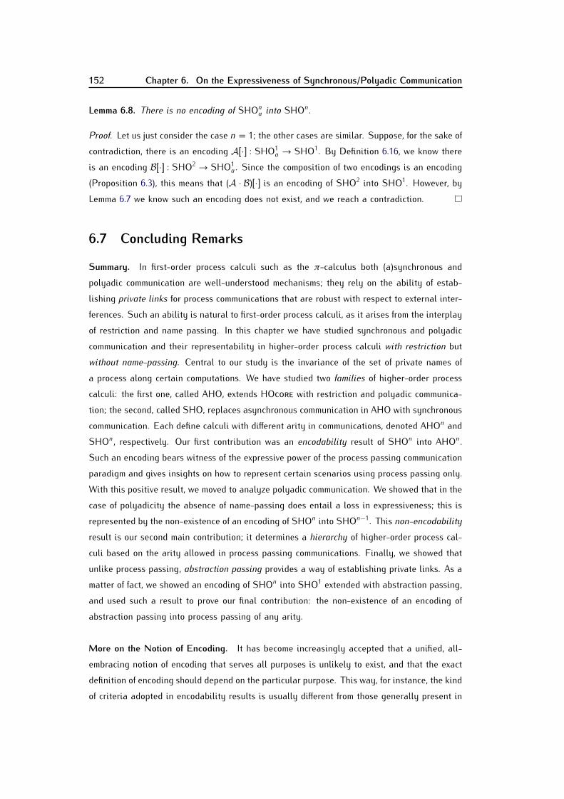
152 Chapter 6. On the Expressiveness of Synchronous/Polyadic Communication
Lemma 6.8. There is no encoding of SHOna into SHOn.Proof. Let us just consider the case n = 1; the other cases are similar. Suppose, for the sake ofcontradiction, there is an encoding A[[·]] : SHO1a → SHO1. By Definition 6.16, we know thereis an encoding B [[·]] : SHO2 → SHO1a. Since the composition of two encodings is an encoding(Proposition 6.3), this means that (A · B )[[·]] is an encoding of SHO2 into SHO1. However, byLemma 6.7 we know such an encoding does not exist, and we reach a contradiction.6.7 Concluding Remarks
Summary. In first-order process calculi such as the π-calculus both (a)synchronous andpolyadic communication are well-understood mechanisms; they rely on the ability of estab-lishing private links for process communications that are robust with respect to external inter-ferences. Such an ability is natural to first-order process calculi, as it arises from the interplayof restriction and name passing. In this chapter we have studied synchronous and polyadiccommunication and their representability in higher-order process calculi with restriction butwithout name-passing. Central to our study is the invariance of the set of private names ofa process along certain computations. We have studied two families of higher-order processcalculi: the first one, called AHO, extends HOCORE with restriction and polyadic communica-tion; the second, called SHO, replaces asynchronous communication in AHO with synchronouscommunication. Each define calculi with different arity in communications, denoted AHOn andSHOn, respectively. Our first contribution was an encodability result of SHOn into AHOn.Such an encoding bears witness of the expressive power of the process passing communicationparadigm and gives insights on how to represent certain scenarios using process passing only.With this positive result, we moved to analyze polyadic communication. We showed that in thecase of polyadicity the absence of name-passing does entail a loss in expressiveness; this isrepresented by the non-existence of an encoding of SHOn into SHOn−1. This non-encodabilityresult is our second main contribution; it determines a hierarchy of higher-order process cal-culi based on the arity allowed in process passing communications. Finally, we showed thatunlike process passing, abstraction passing provides a way of establishing private links. As amatter of fact, we showed an encoding of SHOn into SHO1 extended with abstraction passing,and used such a result to prove our final contribution: the non-existence of an encoding ofabstraction passing into process passing of any arity.More on the Notion of Encoding. It has become increasingly accepted that a unified, all-embracing notion of encoding that serves all purposes is unlikely to exist, and that the exactdefinition of encoding should depend on the particular purpose. This way, for instance, the kindof criteria adopted in encodability results is usually different from those generally present in

6.7. Concluding Remarks 153
separation results. In this chapter we have adopted a notion of encoding that is arguably moredemanding than those previously proposed in the literature for separation results. We arguethat such a definition is in line with our overall goal, that of assessing the expressiveness ofhigher-order concurrency with respect to (a)synchrony and polyadicity and, most importantly,in the absence of name passing.Interferences are a major concern in our setting, essentially because the absence of namepassing leaves us without suitable mechanisms for establishing private links. Devising adefinition of encoding so as to incorporate a notion of potentially malicious context (includingtechniques for reasoning over every possible context) appears very challenging. To this end, wecombine suitable elements from the operational semantics and from the definition of encoding.It could be rightly argued that not all interferences are necessarily harmful, and in this senseour approach to interference handling would appear too coarse. We would like to stress onthe difficulties inherent to only considering interferences; attempting to both considering andhandling them in a selective way seems much more challenging. Also, even if we do notactually prove that encodings behave correctly under every possible context, we think that ourapproach is an initial effort in that direction.Notice that we do not claim our notion of encoding should be taken as a reference for otherseparation results; it simply intends to capture the rather strong correctness requirements(i.e. compositionality and robustness with respect to interferences) which we consider appro-priate and relevant in the restricted setting we are working on. Similarly, we believe that astrict comparison between our notion of encoding and recent proposals for “good” encodingswould not be fair: while it is clear that the “quality” of an encoding will always be an issue,such proposals should be taken primarily as a reference. Our interest is not in introducing anew notion of encoding but in deepening our understanding of the process-passing paradigmand its expressive power. Consequently, we feel that our results should not be judged solelyon the basis of conformance to the requirements of some “good” notion of encoding.Future Work. There are a number of directions worth investigating. An immediate issue isto explore whether the hierarchy of expressiveness for polyadic communication presented inSection 6.5 holds for a less contrained definition of encoding. Here we have focused on derivingthe impossibility result based on the invariance of private names along certain computations;it remains to be explored if other approaches to the separation result, in particular those basedon experiments and divergence as in testing semantics (De Nicola and Hennessy, 1984), couldallow for a proof with a less constrained definition of encoding. We wish to insist that thechallenge is to find a notion that enforces the same correctness guarantees as the ones wehave aimed to enforce here. Clearly, more relaxed conditions in the definition of encodingwould give more significance to our results. Unfortunately, up to now we have been unable toprove the separation results using a less constrained definition.
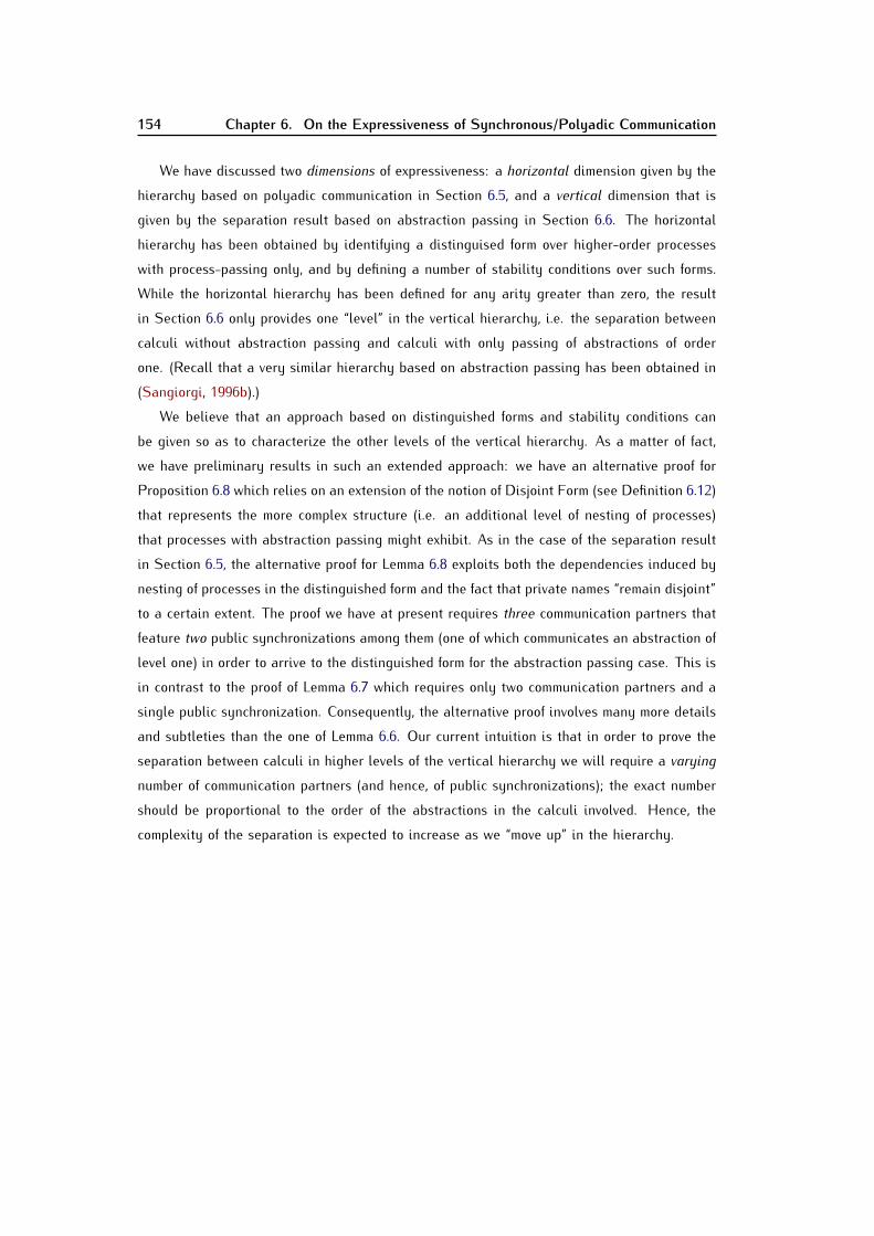
154 Chapter 6. On the Expressiveness of Synchronous/Polyadic Communication
We have discussed two dimensions of expressiveness: a horizontal dimension given by thehierarchy based on polyadic communication in Section 6.5, and a vertical dimension that isgiven by the separation result based on abstraction passing in Section 6.6. The horizontalhierarchy has been obtained by identifying a distinguised form over higher-order processeswith process-passing only, and by defining a number of stability conditions over such forms.While the horizontal hierarchy has been defined for any arity greater than zero, the resultin Section 6.6 only provides one “level” in the vertical hierarchy, i.e. the separation betweencalculi without abstraction passing and calculi with only passing of abstractions of orderone. (Recall that a very similar hierarchy based on abstraction passing has been obtained in(Sangiorgi, 1996b).)We believe that an approach based on distinguished forms and stability conditions canbe given so as to characterize the other levels of the vertical hierarchy. As a matter of fact,we have preliminary results in such an extended approach: we have an alternative proof forProposition 6.8 which relies on an extension of the notion of Disjoint Form (see Definition 6.12)that represents the more complex structure (i.e. an additional level of nesting of processes)that processes with abstraction passing might exhibit. As in the case of the separation resultin Section 6.5, the alternative proof for Lemma 6.8 exploits both the dependencies induced bynesting of processes in the distinguished form and the fact that private names “remain disjoint”to a certain extent. The proof we have at present requires three communication partners thatfeature two public synchronizations among them (one of which communicates an abstraction oflevel one) in order to arrive to the distinguished form for the abstraction passing case. This isin contrast to the proof of Lemma 6.7 which requires only two communication partners and asingle public synchronization. Consequently, the alternative proof involves many more detailsand subtleties than the one of Lemma 6.6. Our current intuition is that in order to prove theseparation between calculi in higher levels of the vertical hierarchy we will require a varyingnumber of communication partners (and hence, of public synchronizations); the exact numbershould be proportional to the order of the abstractions in the calculi involved. Hence, thecomplexity of the separation is expected to increase as we “move up” in the hierarchy.

Chapter 7
Conclusions and Perspectives
7.1 Concluding Remarks
Expressiveness and decidability have been little studied in the context of calculi for higher-order concurrency. In this dissertation we take a direct and minimal approach to the expressive-ness and decidability of higher-order process calculi. This approach finds justification in thefact that higher-order process calculi with specialized operators or modeling features often donot admit a satisfactory interpretation into some first-order setting. The results in this disser-tation concern issues which can be regarded as basic in process calculi, namely (a)synchrony,polyadicity, forwarding. As such, our contributions might have a potential repercussion in thedefinition of a large class of higher-order process calculi.A first achievement of our research is the introduction of HOCORE as a core calculus forhigher-order concurrency. In fact, HOCORE provides a convenient framework to study funda-mental issues of higher-order process calculi: it is minimal enough so as to be theoreticallytractable and, at the same time, it is expressive enough so as to represent interesting phe-nomena in higher-order concurrency. In our opinion, HOCORE can be regarded as the simplest,non-trivial process calculus featuring higher-order concurrency.The most salient feature of HOCORE is the absence of name passing in communications.Given the prominent role of name passing within calculi for concurrency, and the fact thatmost known higher-order process calculi feature both name and process passing, this could bewell considered as the main design decision in our research. The absence of name passing isnecessary to isolate the behavior associated to process passing; as such, it allows to obtainmore accurate assessments of the expressiveness of the process-passing paradigm. In thissense, the results in this dissertation not only deepen our understanding of process-passingcommunication but they can also be interpreted as indirect evidence of the expressiveness andsignificance of the name-passing communication discipline.
156 Chapter 7. Conclusions and Perspectives
It is worth observing that even in the absence of name passing, process-passing is a veryexpressive paradigm. This is demonstrated by the fact that HOCORE, HO−f (the fragment ofHOCORE with limited forwarding), and HOP−f (the extension of HO−f with passivation) areall shown to be Turing complete by exhibiting encodings of Minsky machines. Remarkably,HOCORE and its variants do not have operators for infinite behavior. All the encodings ofMinsky machines presented in this dissertation are compact and intuitive, and exploit con-venient modelling idioms such as input-guarded replication and disjoint sum which canbe expressed succinctly with process-passing only (see Chapters 3 and 5). Another resulton the expressive power of process-passing presented in the dissertation is the encoding ofsynchronous into asynchronous communication presented in Chapter 6 for AHO, the extensionof HOCORE with restriction and polyadic communication.Closely related to the absence of name passing is the treatment of restriction. Restrictionis a practically important construct, as it provides a way of enforcing modelling principlessuch as encapsulation and abstraction into specifications. Along the dissertation, the ab-sence/presence of restriction has shown to have a notable influence on our developments. Theabsence of restriction makes HOCORE a public calculus in which behavior is completely ex-posed; in Chapter 4 we use this to show that Input-Output bisimilarity characterizes τ actions,a necessary step in showing decidability of strong bisimilarity. Also, the absence of restrictionwas useful when deriving an axiomatization of strong bisimilarity, as it allowed to adapt pre-vious results by Moller (1989), Milner and Moller (1993), and Hirschkoff and Pous (2007) for(first-order) calculi without restriction. Also in Chapter 4 we analyzed top-level restrictions,and showed that when HOCORE is extended with four of such restrictions strong bisimilarityis no longer decidable.The results in Chapter 5 are also insightful with respect to restriction. There, we show thatin HO−f termination is decidable whereas convergence is undecidable. While undecidablityof convergence is shown by exhibiting a unfaithful encoding of Minsky machines, we areable to prove decidability of termination by appealing the theory of well-structured transitionsystems. To our knowledge, ours is the first application of such theory in the higher-ordersetting. HO−f is a calculus without restriction and yet it has the same decidability propertiesof CCSν! , the variant of CCS with restriction and replication as the only source of infinitebehavior. Indeed, also in CCSν! termination is decidable and convergence is undecidable (Busiet al., 2009). We find this surprising because it is well-known that in fragments of CCS withoutrestriction decision problems such as termination and convergence of processes are decidable.1This observation on the presence of restriction also bears witness of the expressiveness of1In fact, Goltz (1988) has shown that the fragment of CCS without restriction and relabeling can be translatedinto a strongly bisimilar finite Petri net. Since termination and convergence are decidable for finite Petri nets (see,e.g., (Esparza and Nielsen, 1994))and strong bisimilarity preserves both propertieswe can conclude that bothtermination and convergence are decidable in such a fragment of CCS.

7.2. Ongoing and Future Work 157
process-passing. Furthermore, the expressiveness results for HOP−f given in Chapter 5 canbe alternatively interpreted from the point of view of restriction. In fact, passivation as wedefine it here adds a subtle notion of structure to higher-order processes. This reminds usof the role of restriction in expressiveness studies for other process calculi. In that sense,passivation can be considered as a very relaxed form of restriction. It is worth noticing thatthe addition of passivation to HO−f allows to describe a faithful encoding of Minsky machines,thus showing that both convergence and termination are undecidable in HOP−f . The notion ofstructure on processes induced by passivation units is therefore crucial to both expressivenessand decidability of HOP−f .Finally, in Chapter 6 we consider extensions of HOCORE with full (i.e., ordinary) restriction.There, we discussed how the scope extrusion one obtains with restriction but without name-passing is incomplete in that (restricted) names can be passed around inside processes butcannot be effectively used within of receiving context. As a result, with only process-passingit is not possible to establish private links as those used in encodings of synchronous andpolyadic communication in first-order calculi. This insight is central to the separation resultsfor SHO (i.e., the synchronous variant of AHO). By combining selected features from a moreinformative LTS and a rather demanding notion of encoding we were able to show that SHOn
(i.e. the instance of SHO with n-adic communication) cannot be encoded into SHOn−1, thusdetermining a hierarchy of higher-order process calculi based on polyadicity. This resultsuggests that in the absence of the name-passing, the impact of adding restriction diminishes.The last result in Chapter 6 shows that the ability of establishing private links in SHO (thatis, the ability of fully exploiting restriction and restricted names) is obtained when extendingSHO with abstraction-passing. This is an insightful result, in that abstraction is arguably oneof the most practically useful constructs in the higher-order π-calculus.Along the dissertation we describe the way in which basic modeling idioms such as lists,counters, and constructs for choice and guarded infinite behavior can be expressed in corehigher-order process calculi. Nevertheless, this does not seem enough so as to consider corehigher-order process calculi as adequate as modelling languages in concrete application areas.In our opinion, higher-order process calculi for specialized application areas should arise fromthe careful combination of higher-order constructs and name-passing features.
7.2 Ongoing and Future Work
Along the dissertation we have already pointed out a number of strands for future work. Weconclude by commenting on those directions we find particularly promising; some of them areobject of current work.
158 Chapter 7. Conclusions and Perspectives
More on Expressiveness of Passivation. In Chapter 5 we have examined the expressivenessassociated to suspension operators by studying the influence a passivation operator has on theabsolute expressive power of a higher-order process calculus with restricted output actions.In this respect, much remains to be done. In fact, we have considered a particular form ofpassivation, one that allows to both suspend a process and then restart it later. Other formsof passivation (more precisely, other semantics for passivation) are also possible and couldbe relevant. A natural concern is that, as we pointed out before, passivation as defined herehas a very non-deterministic character. It is reasonable to assume that the kind of passivationrequired for applications in dynamic system reconfiguration to be more controlled.We have conducted preliminary studies on the expressiveness of passivation in the contextof aCCS−ν! , the asynchronous fragment of CCS without restriction and with replication (DiGiusto et al., 2009b). In the absence of process-passing a passivation action entails essentiallythe destruction of the content of the passivation unit. That is, suspension represents a “kill”action over a process. We think that this “destructive passivation” is perhaps the simplest kindof passivation one could think of. In (Di Giusto et al., 2009b) we show that even destructivepassivation is enough to increase the expressive power of aCCS−ν! . Using the same theoreticalmachinery as in Chapter 5 (i.e. unfaithful encodings of Minsky machines and well-structuredtransition systems) we show that in aCCS−ν! extended with passivation: (i) in contrast to thesituation in aCCS−ν! , convergence is undecidable; and (ii) similarly as in aCCS−ν! , terminationis decidable.Higher-Order and Ambient-like Calculi. Ambient-like and higher-order process calculi aresimilar in that they involve complex objects in interactions. Also, in both cases the associatedbehavioral theory can be hard to define, and employs similar techniques. However, someother characteristics suggest deep differences. Communication in Ambients resembles a “move”operation whereas in higher-order settings it is better assimilated to a “copy” operation. Mostnotably, there is a subtle discrepancy when it comes to binding: most (higher-order) processcalculi adopt static binding only, whereas Ambient-like formalisms exhibit features of bothstatic and dynamic binding.Based on the above, we find it interesting to formally compare Ambient-like and higher-order calculi. From the point of view of expressiveness, this is relevant for at least two reasons.First, in the light of the above differences, an encoding of Ambient calculi would representa significant test of expressiveness for the process-passing paradigm. Second, it would shedlight on the intrinsic nature of the Ambient primitives which have proven so successful.In (Di Giusto and Perez, 2009) we have reported on initial results of our investigation: anencoding of Ambient calculus into a higher-order process calculi with localities (implementedas passivation units) and a form of dynamic binding. The encoding is useful to understandthe nature of Ambient communication; it also allows us to conjecture that an encoding into

7.2. Ongoing and Future Work 159
a higher-order process calculus with static binding does not exist. It would be interestingto see whether this encodability result can be exploited/strengthened so as to have a moreconclusive assessment of the expressiveness of the higher-order paradigm with respect to theAmbient calculi. Also, it is not clear how to proceed in order to transform our conjecture intoa formal separation result. It could be that passivation and dynamic binding crucial in theencoding in (Di Giusto and Perez, 2009) could give hints in this case, but this remains tobe explored in detail.Dimensions of Mobility. Together with Roland Meyer, we are studying the relationship be-tween decidability results for the π-calculus and those presented in Chapter 5 for HO−f . Inhis PhD Thesis, Meyer (2008) studied the notion of structural stationarity in the π-calculus.Roughly speaking, structural stationarity means bounding processes so as to obtain decid-ability results and hence perform automatic verification techniques on them. In the π-calculus,structural stationarity arises by giving bounds on two dimensions of infinite behavior: depth(i.e., the nesting of restrictions inside a process) and breadth (i.e., the degree of parallelism ofa process). It would be interesting to determine precisely what structural stationarity meansfor higher-order processes, and its exact relationship with that in the first-order setting. Inprinciple, such a relationship should allow to transfer and generalize decidability results fromone setting to the other.


References
ABADI, M. AND FOURNET, C. 2001. Mobile values, new names, and secure communication. InProc. of POPL’01. ACM, 104–115. 43ABADI, M. AND GORDON, A. D. 1999. A calculus for cryptographic protocols: The spi calculus.Inf. Comput. 148, 1, 1–70. 34, 43ABDULLA, P. A., CERANS, K., JONSSON, B., AND TSAY, Y.-K. 2000. Algorithmic analysis ofprograms with well quasi-ordered domains. Inf. Comput. 160, 1-2, 109–127. 50, 93, 124ABRAMSKY, S. 1989. The lazy lambda calculus. In Research Topics in Functional Program-ming, D. Turner, Ed. Addison Wesley, Reading, MA., 65–116. 31, 34AMADIO, R. M. 1993. On the reduction of chocs bisimulation to pi-calculus bisimulation.In Proc. of CONCUR. Lecture Notes in Computer Science, vol. 715. Springer, 112–126.Extended version available in the author’s web site. 52, 132AMADIO, R. M. 1994. Translating core facile. Tech. Rep. ECRC-94-3, ECRC, Munich. 52AMADIO, R. M., CASTELLANI, I., AND SANGIORGI, D. 1998. On bisimulations for the asynchronouspi-calculus. Theor. Comput. Sci. 195, 2, 291–324. 74AMADIO, R. M., LETH, L., AND THOMSEN, B. 1995. From a concurrent lambda-calculus tothe pi-calculus. In Proc. of FCT. Lecture Notes in Computer Science, vol. 965. Springer,106–115. 52ARANDA, J., GIUSTO, C. D., NIELSEN, M., AND VALENCIA, F. D. 2007. Ccs with replication in thechomsky hierarchy: The expressive power of divergence. In Proc. of APLAS. Lecture Notesin Computer Science, vol. 4807. Springer, 383–398. 48ARANDA, J. A. 2009. On the expressivity of infinite and local behaviour in fragments of thepi-calculus. Ph.D. thesis, Ecole Polytechnique de Paris and Universidad del Valle Colombia.39, 49
162 References
ASTESIANO, E., GIOVINI, A., AND REGGIO, G. 1988. Generalized bisimulation in relationalspecifications. In Proc. of STACS. Lecture Notes in Computer Science, vol. 294. Springer,207–226. 35BALDAMUS, M. 1998. Semantics and logic of higher-order processes: Characterizing latecontext bisimulation. Ph.D. thesis, Computer science department, Berlin University of Tech-nology. 36BARENDREGT, H. 1984. The Lambda Calculus: Its Syntax and Semantics. North-Holland. 51BEAUXIS, R., PALAMIDESSI, C., AND VALENCIA, F. D. 2008. On the asynchronous nature of theasynchronous pi-calculus. In Concurrency, Graphs and Models. Lecture Notes in ComputerScience, vol. 5065. Springer, 473–492. 12, 46, 131BERNSTEIN, K. L. 1998. A congruence theorem for structured operational semantics of higher-order languages. In Proc. of LICS’98. IEEE Computer Society, 153–164. 37BLOOM, B. 1994. Chocolate: Calculi of higher order communication and lambda terms. InProc. of POPL’94. ACM, 339–347. 31BOREALE, M., DE NICOLA, R., AND PUGLIESE, R. 1999. Basic observables for processes. Inf.Comput. 149, 1, 77–98. 33BOUDOL, G. 1989. Towards a lambda-calculus for concurrent and communicating systems. InProc. of TAPSOFT, Vol.1. Lecture Notes in Computer Science, vol. 351. Springer, 149–161.Also appeared as INRIA Research Report No. RR-0885, August 1988. 5, 29, 30, 31, 35BOUDOL, G. 1992. Asynchrony and the π-calculus (note). Tech. rep., Rapport de Recherche1702, INRIA, Sophia-Antipolis. 11, 42, 128BOUDOL, G. 1998. The pi-calculus in direct style. Higher-Order and Symbolic Computa-tion 11, 2, 177–208. A preliminary version appeared in Proc. of POPL’97. 31, 32BOUGE, L. 1988. On the existence of symmetric algorithms to find leaders in networks ofcommunicating sequential processes. Acta Inf. 25, 2, 179–201. 42, 50BRAVETTI, M. AND ZAVATTARO, G. 2009. On the expressive power of process interruption andcompensation. Math. Struct. in Comp. Sci. 19, 3, 565–599. 48, 92, 124BUNDGAARD, M., GLENSTRUP, A. J., HILDEBRANDT, T. T., HØJSGAARD, E., AND NISS, H. 2008.Formalizing higher-order mobile embedded business processes with binding bigraphs. InProc. of COORDINATION. Lecture Notes in Computer Science, vol. 5052. Springer, 83–99.118

References 163
BUNDGAARD, M., GODSKESEN, J. C., HAAGENSEN, B., AND HUTTEL, H. 2009. Decidable fragmentsof a higher order calculus with locations. Electr. Notes Theor. Comput. Sci. 242, 1, 113–138.10, 54, 125BUNDGAARD, M., HILDEBRANDT, T. T., AND GODSKESEN, J. C. 2006. A cps encoding of name-passing in higher-order mobile embedded resources. Theor. Comput. Sci. 356, 3, 422–439.10, 54BUSI, N., GABBRIELLI, M., AND ZAVATTARO, G. 2003. Replication vs. recursive definitions inchannel based calculi. In Proc. of ICALP. Lecture Notes in Computer Science, vol. 2719.Springer, 133–144. 64BUSI, N., GABBRIELLI, M., AND ZAVATTARO, G. 2009. On the expressive power of recursion,replication and iteration in process calculi. Math. Struct. in Comp. Sci. 19, 6, 1191–1222.18, 47, 49, 50, 64, 93, 95, 124, 156BUSI, N., GORRIERI, R., AND ZAVATTARO, G. 2000. On the expressiveness of linda coordinationprimitives. Inf. Comput. 156, 1-2, 90–121. Full version of a paper in Proc. of EXPRESS’97.47, 50BUSI, N. AND ZANDRON, C. 2009. Computational expressiveness of genetic systems. Theor.Comput. Sci. 410, 4-5, 286–293. 39BUSI, N. AND ZAVATTARO, G. 2000. On the expressiveness of event notification in data-drivencoordination languages. In Proc. of ESOP. Lecture Notes in Computer Science, vol. 1782.Springer, 41–55. 47BUSI, N. AND ZAVATTARO, G. 2004. On the expressive power of movement and restriction inpure mobile ambients. Theor. Comput. Sci. 322, 3, 477–515. 47, 64, 125CACCIAGRANO, D., CORRADINI, F., AND PALAMIDESSI, C. 2007. Separation of synchronous andasynchronous communication via testing. Theor. Comput. Sci. 386, 3, 218–235. 12, 43, 131CAO, Z. 2006. More on bisimulations for higher order pi-calculus. In Proc. of FoSSaCS’06.Lecture Notes in Computer Science, vol. 3921. Springer, 63–78. 35, 74CARBONE, M. AND MAFFEIS, S. 2003. On the expressive power of polyadic synchronisation inpi-calculus. Nord. J. Comput. 10, 2, 70–98. 51CARDELLI, L. AND GORDON, A. D. 2000. Mobile ambients. Theor. Comput. Sci. 240, 1, 177–213.A preliminary version appeared in Proc. of FOSSACS’98. 5, 7, 32, 47, 125CHANDRA, A. K. AND MANNA, Z. 1976. On the power of programming features. Comput.Lang. 1, 3, 219–232. 40
164 References
CHRISTENSEN, S. 1993. PhD thesis CST–105–93. Ph.D. thesis, Dept. of Computer Science,University of Edinburgh. 47CHRISTENSEN, S., HIRSHFELD, Y., AND MOLLER, F. 1994. Decidable subsets of CCS. Comput.J. 37, 4, 233–242. 89COLLBERG, C. S., THOMBORSON, C. D., AND LOW, D. 1998. Manufacturing cheap, resilient, andstealthy opaque constructs. In Proc. of POPL’98. ACM Press, 184–196. 93DE BOER, F. S. AND PALAMIDESSI, C. 1990. Concurrent logic programming: Asynchronism andlanguage comparison. In Proc. of NACLP. The MIT Press, Series in Logic Programming,175–194. 41DE BOER, F. S. AND PALAMIDESSI, C. 1991. Embedding as a tool for language comparison:On the csp hierarchy. In Proc. of CONCUR. Lecture Notes in Computer Science, vol. 527.Springer, 127–141. 42DE BOER, F. S. AND PALAMIDESSI, C. 1994. Embedding as a tool for language comparison.Inf. Comput. 108, 1, 128–157. 41, 42DE BRUIJN, N. G. 1972. Lambda calculus notation with nameless dummies: A tool forautomatic formula manipulation, with application to the church-rosser theorem. IndagationesMathematicae 34, 381–392. 82DE NICOLA, R. 2006. From process calculi to Klaim and back. Electr. Notes Theor. Comput.Sci. 162, 159–162. 33DE NICOLA, R., FERRARI, G. L., AND PUGLIESE, R. 1998. Klaim: A kernel language for agentsinteraction and mobility. IEEE Trans. Software Eng. 24, 5, 315–330. 33DE NICOLA, R. AND HENNESSY, M. 1984. Testing equivalences for processes. Theor. Comput.Sci. 34, 83–133. 15, 46, 153DE SIMONE, R. 1985. Higher-level synchronising devices in meije-sccs. Theor. Comput.Sci. 37, 245–267. 39, 52DEMANGEON, R., HIRSCHKOFF, D., AND SANGIORGI, D. 2010. Termination in higher-orderconcurrent calculi. In Proc. of FSEN’09. Lecture Notes in Computer Science, vol. 5961.Springer, 81–96. 11DI GIUSTO, C. AND PEREZ, J. A. 2009. Move vs copy: Towards a formal comparision of ambientsand higher-order process calculi. In Proc. of ICTCS’09: the Eleventh Italian Conference onTheoretical Computer Science. 158, 159

References 165
DI GIUSTO, C., PEREZ, J. A., AND ZAVATTARO, G. 2009a. On the expressiveness of forwardingin higher-order communication. In Proc. of ICTAC. Lecture Notes in Computer Science, vol.5684. Springer, 155–169. 14, 91DI GIUSTO, C., PEREZ, J. A., AND ZAVATTARO, G. 2009b. On the expressiveness of suspensionin higher-order process calculi. In preparation. 158DOVIER, A., PIAZZA, C., AND POLICRITI, A. 2004. An efficient algorithm for computing bisimu-lation equivalence. Theor. Comput. Sci. 311, 1-3, 221–256. 81DSOUZA, A. AND BLOOM, B. 1995. On the expressive power of ccs. In Proc. of FSTTCS.Lecture Notes in Computer Science, vol. 1026. Springer, 309–323. 52DUFOURD, C., FINKEL, A., AND SCHNOEBELEN, P. 1998. Reset nets between decidability andundecidability. In Proc. of ICALP. Lecture Notes in Computer Science, vol. 1443. Springer,103–115. 50ENE, C. AND MUNTEAN, T. 1999. Expressiveness of point-to-point versus broadcast communi-cations. In Proc. of FCT. Lecture Notes in Computer Science, vol. 1684. Springer, 258–268.43, 50ESPARZA, J. AND NIELSEN, M. 1994. Decidability issues for petri nets - a survey. Bulletin ofthe EATCS 52, 244–262. 156FELLEISEN, M. 1991. On the expressive power of programming languages. Sci. Comput.Program. 17, 1-3, 35–75. A preliminary version appeared in Proc. of ESOP’90. 40, 46FERREIRA, W., HENNESSY, M., AND JEFFREY, A. 1998. A theory of weak bisimulation for corecml. J. Funct. Program. 8, 5, 447–491. 36FINKEL, A. 1990. Reduction and covering of infinite reachability trees. Inf. Comput. 89, 2,144–179. 50, 93, 124FINKEL, A. AND SCHNOEBELEN, P. 2001. Well-structured transition systems everywhere!Theor. Comput. Sci. 256, 1-2, 63–92. 50, 93, 105, 106, 124FOURNET, C., GONTHIER, G., LEVY, J.-J., MARANGET, L., AND REMY, D. 1996. A calculus of mobileagents. In Proc. of CONCUR. Lecture Notes in Computer Science, vol. 1119. Springer, 406–421. 32GIACALONE, A., MISHRA, P., AND PRASAD, S. 1989. Facile: A symmetric integration of concur-rent and functional programming. In Proc. of TAPSOFT, Vol.2. Lecture Notes in ComputerScience, vol. 352. Springer, 184–209. 30

166 References
GODSKESEN, J. C. AND HILDEBRANDT, T. T. 2005. Extending howe’s method to early bisimula-tions for typed mobile embedded resources with local names. In Proc. of FSTTCS. LectureNotes in Computer Science, vol. 3821. Springer, 140–151. 36GOLTZ, U. 1988. On representing ccs programs by finite petri nets. In Proc. of MFCS. LectureNotes in Computer Science, vol. 324. Springer, 339–350. 156GORLA, D. 2006. Comparing calculi for mobility via their relative expressive power. Tech.Rep. 09/2006, Dipartimento di Informatica, Universita di Roma - La Sapienza. 46GORLA, D. 2008. Towards a unified approach to encodability and separation results for processcalculi. In Proc. of CONCUR. Lecture Notes in Computer Science, vol. 5201. Springer, 492–507. Extended version available as Tech. Rep. 10/2008, Dip. Informatica, Universita di Roma- La Sapienza. 43, 46, 135HENNESSY, M., RATHKE, J., AND YOSHIDA, N. 2005. safedpi: a language for controlling mobilecode. Acta Inf. 42, 4-5, 227–290. 34HIGMAN, G. 1952. Ordering by divisibility in abstract algebras. Proceedings of the LondonMathematical Society (3) 2, 7, 326–336. 106HILDEBRANDT, T., GODSKESEN, J. C., AND BUNDGAARD, M. 2004. Bisimulation congruences forHomer a calculus of higher order mobile embedded resources. Tech. Rep. TR-2004-52, ITUniversity of Copenhagen. 9, 10, 29, 33, 36, 118, 125HIRSCHKOFF, D., LOZES, E., AND SANGIORGI, D. 2002. Separability, expressiveness, and de-cidability in the ambient logic. In Proc. of LICS’02. IEEE Computer Society Press, 423–432.47HIRSCHKOFF, D. AND POUS, D. 2007. A distribution law for CCS and a new congruence resultfor the pi-calculus. In Proc. of FoSSaCS’07. Lecture Notes in Computer Science, vol. 4423.Springer, 228–242. 78, 79, 156HONDA, K. AND TOKORO, M. 1991. An object calculus for asynchronous communication. InProc. of ECOOP. Lecture Notes in Computer Science, vol. 512. Springer, 133–147. 11, 42,128HONDA, K., VASCONCELOS, V. T., AND KUBO, M. 1998. Language primitives and type disciplinefor structured communication-based programming. In Proc. of ESOP. Lecture Notes inComputer Science, vol. 1381. Springer, 122–138. 4, 43HONDA, K. AND YOSHIDA, N. 1994a. Combinatory representation of mobile processes. In Proc.of POPL’94. ACM, 348–360. 51

References 167
HONDA, K. AND YOSHIDA, N. 1994b. Replication in concurrent combinators. In Proc. of TACS.Lecture Notes in Computer Science, vol. 789. Springer, 786–805. 51HONDA, K. AND YOSHIDA, N. 1995. On reduction-based process semantics. Theor. Comput.Sci. 151, 2, 437–486. 74HOWE, D. J. 1996. Proving congruence of bisimulation in functional programming languages.Inf. Comput. 124, 2, 103–112. 36, 70JEFFREY, A. AND RATHKE, J. 2005. Contextual equivalence for higher-order pi-calculus revis-ited. Logical Methods in Computer Science 1, 1, 1–22. 35, 36, 67KOUTAVAS, V. AND HENNESSY, M. 2009. First-order reasoning for higher-order concurrency.Tech. rep., Trinity College Dublin. July. 36KUCERA, A. AND JANCAR, P. 2006. Equivalence-checking on infinite-state systems: Techniquesand results. TPLP 6, 3, 227–264. 89, 90LANDIN, P. J. 1966. The Next 700 Programming Languages. Communications of the ACM 9, 3(March), 157–166. 40LANESE, I. 2007. Concurrent and located synchronizations in pi-calculus. In Proc. of SOF-SEM. Lecture Notes in Computer Science, vol. 4362. Springer, 388–399. 131LANESE, I., PEREZ, J. A., SANGIORGI, D., AND SCHMITT, A. 2008. On the expressiveness anddecidability of higher-order process calculi. In Proc. of LICS’08. IEEE Computer Society,145–155. 14LANESE, I., PEREZ, J. A., SANGIORGI, D., AND SCHMITT, A. 2009. On the expressiveness anddecidability of polyadicity in higher-order process calculi (extended abstract). In Proc. ofICTCS’09: the Eleventh Italian Conference on Theoretical Computer Science. 14, 127LANEVE, C. AND VICTOR, B. 2003. Solos in concert. Mathematical Structures in ComputerScience 13, 5, 657–683. 51LENGLET, S., SCHMITT, A., AND STEFANI, J.-B. 2008. Bisimulations in calculi featuring passi-vation and restriction. Technical Report, Sardes Project, INRIA Rhone Alpes. 11, 37LENGLET, S., SCHMITT, A., AND STEFANI, J.-B. 2009a. Howe’s method for calculi with passiva-tion. In Proc. of CONCUR. Lecture Notes in Computer Science, vol. 5710. Springer, 448–462.37LENGLET, S., SCHMITT, A., AND STEFANI, J.-B. 2009b. Normal bisimulations in calculi withpassivation. In Proc. of FOSSACS. Lecture Notes in Computer Science, vol. 5504. Springer,257–271. 37

168 References
MAFFEIS, S., ABADI, M., FOURNET, C., AND GORDON, A. D. 2008. Code-carrying authorization.In Proc. of ESORICS. Lecture Notes in Computer Science, vol. 5283. Springer, 563–579. 34MAFFEIS, S. AND PHILLIPS, I. 2005. On the computational strength of pure ambient calculi.Theor. Comput. Sci. 330, 3, 501–551. 47, 48MAYR, R. 2000. Process rewrite systems. Inf. Comput. 156, 1-2, 264–286. 48MEREDITH, L. G. AND RADESTOCK, M. 2005a. Namespace logic: A logic for a reflective higher-order calculus. In Proc. of TGC. Lecture Notes in Computer Science, vol. 3705. Springer,353–369. 34MEREDITH, L. G. AND RADESTOCK, M. 2005b. A reflective higher-order calculus. Electr. NotesTheor. Comput. Sci. 141, 5, 49–67. 34MEYER, R. 2008. Structural stationarity in the pi-calculus. Ph.D. thesis, Department ofComputing Science, University of Oldenburg. 159MILNER, R. 1989. Communication and Concurrency. International Series in Computer Science.Prentice Hall. 15, 17, 19, 25, 67MILNER, R. 1991. The Polyadic pi-Calculus: A Tutorial. Tech. Rep. ECS-LFCS-91-180,University of Edinburgh. 23, 42, 128MILNER, R. 1992. Functions as processes. Mathematical Structures in Computer Science 2, 2,119–141. 4, 52MILNER, R. AND MOLLER, F. 1993. Unique decomposition of processes. Theor. Comput.Sci. 107, 2, 357–363. 78, 156MILNER, R., PARROW, J., AND WALKER, D. 1992. A calculus of mobile processes, i. Inf. Com-put. 100, 1, 1–40. A preliminary version appeared as Technical Report ECS-LFCS-89-85,LFCS, University of Edinburgh, June 1989. 4, 15, 22, 31MILNER, R. AND SANGIORGI, D. 1992. Barbed bisimulation. In Proc. 19th ICALP, W. Kuich,Ed. Lecture Notes in Computer Science, vol. 623. Springer Verlag, 685–695. 20, 46, 74MINSKY, M. 1967. Computation: Finite and Infinite Machines. Prentice-Hall. 47, 49MITCHELL, J. C. 1993. On abstraction and the expressive power of programming languages.Sci. Comput. Program. 21, 2, 141–163. 40MOLLER, F. 1989. Axioms for concurrency. Ph.D. thesis, University of Edinburgh, Dept. ofComp. Sci. PhD thesis CST–59–89. 78, 156
References 169
MOLLER, F. 1996. Infinite results. In Proc. of CONCUR. Lecture Notes in Computer Science,vol. 1119. Springer, 195–216. 48MOSTROUS, D. AND YOSHIDA, N. 2007. Two session typing systems for higher-order mobileprocesses. In Proc. of TLCA. Lecture Notes in Computer Science, vol. 4583. Springer, 321–335. 34MOSTROUS, D. AND YOSHIDA, N. 2009. Session-based communication optimisation for higher-order mobile processes. In Proc. of TLCA. Lecture Notes in Computer Science, vol. 5608.Springer, 203–218. 34MOUSAVI, M. R., GABBAY, M., AND RENIERS, M. A. 2005. SOS for Higher Order Processes. InProc. of CONCUR. Lecture Notes in Computer Science, vol. 3653. Springer, 308–322. 37MOUSAVI, M. R., RENIERS, M. A., AND GROOTE, J. F. 2007. SOS formats and meta-theory: 20years after. Theor. Comput. Sci. 373, 3, 238–272. 37NECULA, G. C. AND LEE, P. 1998. Safe, untrusted agents using proof-carrying code. In MobileAgents and Security. Lecture Notes in Computer Science, vol. 1419. Springer, 61–91. 93NESTMANN, U. 1996. On determinacy and and nondeterminacy in concurrent programming.Ph.D. thesis, Univ. Erlangen. 43, 44NESTMANN, U. 2000. What is a ”good” encoding of guarded choice? Inf. Comput. 156, 1-2,287–319. A preliminary version appeared in EXPRESS’97. 43, 46NESTMANN, U. AND PIERCE, B. C. 2000. Decoding choice encodings. Inf. Comput. 163, 1, 1–59.Extended abstract in Proc. of CONCUR’96. 43, 45NIELSON, F. 1989. The typed lambda-calculus with first-class processes. In Proc. of PARLE(2). Lecture Notes in Computer Science, vol. 366. Springer, 357–373. 5, 29, 30NYGAARD, M. AND WINSKEL, G. 2002. Hopla-a higher-order process language. In Proc. ofCONCUR. Lecture Notes in Computer Science, vol. 2421. Springer, 434–448. 33OSTROVSKY, K., PRASAD, K. V. S., AND TAHA, W. 2002. Towards a primitive higher ordercalculus of broadcasting systems. In Proc. of PPDP. ACM, 2–13. 34PALAMIDESSI, C. 2003. Comparing the expressive power of the synchronous and asynchronouspi-calculi. Mathematical Structures in Computer Science 13, 5, 685–719. Extended abstractin Proc. of POPL’97. 12, 43, 45, 46, 50, 128, 131PARROW, J. 1990. The expressive power of parallelism. Future Gener. Comput. Syst. 6, 3,271–285. 51
170 References
PARROW, J. 2000. Trios in concert. In Proof, Language, and Interaction. The MIT Press,623–638. 51PARROW, J. 2008. Expressiveness of process algebras. Electr. Notes Theor. Comput. Sci. 209,173–186. 37, 39PIERCE, B. AND SANGIORGI, D. 1996. Typing and subtyping for mobile processes. Journal ofMathematical Structures in Computer Science 6, 5, 409–454. An extended abstract appearedin Proc. LICS 93, IEEE Computer Society Press. 23POST, E. L. 1946. A variant of a recursively unsolvable problem. Bull. of the Am. Math.Soc 52, 264–268. 85PRASAD, S., GIACALONE, A., AND MISHRA, P. 1990. Operational and algebraic semantics forfacile: A symmetric integration of concurrent and functional programming. In Proc. of ICALP.Lecture Notes in Computer Science, vol. 443. Springer, 765–778. 30PRIAMI, C. 1995. Stochastic pi-calculus. Comput. J. 38, 7, 578–589. 42, 43QUAGLIA, P. AND WALKER, D. 2005. Types and full abstraction for polyadic pi-calculus. Inf.Comput. 200, 2, 215–246. 43, 131RADESTOCK, M. AND EISENBACH, S. 1996. Semantics of a higher-order coordination language.In Proc. of COORDINATION. Lecture Notes in Computer Science, vol. 1061. Springer, 339–356. 34RAJA, N. AND SHYAMASUNDAR, R. K. 1995a. Combinatory formulations of concurrent languages.In Proc. of ASIAN. Lecture Notes in Computer Science, vol. 1023. Springer, 156–170. 51RAJA, N. AND SHYAMASUNDAR, R. K. 1995b. The quine-bernays combinatory calculus. Int. J.Found. Comput. Sci. 6, 4, 417–430. 51REPPY, J. H. 1991. CML: A higher-order concurrent language. In PLDI. 293–305. 30REPPY, J. H. 1992. Higher-order concurrency. Ph.D. thesis, Cornell University. 30RIECKE, J. G. 1993. Fully abstract translations between functional languages. MathematicalStructures in Computer Science 3, 4, 387–415. A preliminary report appeared in Proc. ofPOPL’91. 41SANGIORGI, D. 1992. Expressing mobility in process algebras: First-order and higher-orderparadigms. Ph.D. thesis, University of Edinburgh. 4, 5, 6, 10, 21, 23, 25, 26, 28, 29, 35, 42,43, 47, 52, 53, 55, 67, 84
References 171
SANGIORGI, D. 1993. From π-calculus to Higher-Order π-calculus and back. In Proc.TAPSOFT’93, M.-C. Gaudel and J.-P. Jouannaud, Eds. Lecture Notes in Computer Science,vol. 668. Springer Verlag, 151–166. 21, 27SANGIORGI, D. 1994. The lazy lambda calculus in a concurrency scenario. Information andComputation 111, 1, 120–153. 34SANGIORGI, D. 1996a. Bisimulation for Higher-Order Process Calculi. Inf. Comput. 131, 2,141–178. 35, 36, 55, 84SANGIORGI, D. 1996b. π-calculus, internal mobility and agent-passing calculi. Theor. Comput.Sci. 167, 2, 235–274. 10, 26, 52, 55, 88, 131, 132, 151, 154SANGIORGI, D. 1996c. A theory of bisimulation for the π-calculus. Acta Informatica 33, 69–97. An extract appeared in Proc. CONCUR ’93, Lecture Notes in Computer Science 715,Springer Verlag. 35SANGIORGI, D. 1998. On the bisimulation proof method. Journal of Mathematical Structuresin Computer Science 8, 447–479. 36SANGIORGI, D. 2001. Asynchronous process calculi: the first-order and higher-orderparadigms (tutorial). Theor. Comput. Sci. 253, 311–350. 27SANGIORGI, D. 2009. An introduction to bisimulation and coinduction. Draft. 16, 19SANGIORGI, D., KOBAYASHI, N., AND SUMII, E. 2007. Environmental bisimulations for higher-order languages. In Proc. of LICS’07. IEEE Computer Society, 293–302. 36, 67SANGIORGI, D. AND WALKER, D. 2001. The π-calculus: a Theory of Mobile Processes. Cam-bridge University Press. 4, 8, 10, 21, 22, 25, 27, 53, 64, 74, 84, 88SATO, N. AND SUMII, E. 2009. The higher-order, call-by-value applied pi-calculus. In Proc.of APLAS’09: the Seventh Asian Symposium on Programming Languages and Systems.Lecture Notes in Computer Science. Springer. To Appear. 11, 34, 36SCHMITT, A. AND STEFANI, J.-B. 2002. The m-calculus: a higher-order distributed processcalculus. Tech. Rep. 4361, INRIA. Jan. 32SCHMITT, A. AND STEFANI, J.-B. 2003. The m-calculus: a higher-order distributed processcalculus. In Proc. of POPL’03. ACM, 50–61. 32SCHMITT, A. AND STEFANI, J.-B. 2004. The kell calculus: A family of higher-order distributedprocess calculi. In Proc. of Global Computing. Lecture Notes in Computer Science, vol. 3267.Springer, 146–178. 9, 29, 32, 118
172 References
SHAPIRO, E. Y. 1989. The family of concurrent logic programming languages. ACM Comput.Surv. 21, 3, 413–510. 41SHAPIRO, E. Y. 1991. Separating concurrent languages with categories of language embed-dings (extended abstract). In Proc. of STOC’91. ACM, 198–208. 41SHAPIRO, E. Y. 1992. Embeddings among concurrent programming languages (preliminaryversion). In Proc. of CONCUR. Lecture Notes in Computer Science, vol. 630. Springer,486–503. 42SHEPHERDSON, J. C. AND STURGIS, H. E. 1963. Computability of recursive functions. J.ACM 10, 2, 217–255. 47SIPSER, M. 2005. Introduction to the Theory of Computation. PWS Publishing Company. 85THOMSEN, B. 1989. A calculus of higher order communicating systems. In Proc. of POPL’89.ACM Press, 143–154. 5, 25, 36, 55, 172THOMSEN, B. 1990. Calculi for higher order communicating systems. Ph.D. thesis, Dept. ofComp. Sci., Imperial College. 10, 25, 29, 30, 31, 35, 42, 54, 84THOMSEN, B. 1993. Plain CHOCS: A second generation calculus for higher order processes.Acta Inf. 30, 1, 1–59. 5, 31, 36, 55THOMSEN, B. 1995. A theory of higher order communicating systems. Inf. Comput. 116, 1,38–57. Extended version of Thomsen (1989). 30VAANDRAGER, F. W. 1992. Expressive results for process algebras. In Proc. of REX Workshopon ‘Semantics: Foundations and Application’. Lecture Notes in Computer Science, vol. 666.Springer, 609–638. Also available as CWI Report CS-R9301, 1993. 52VERSARI, C., BUSI, N., AND GORRIERI, R. 2009. An expressiveness study of priority in processcalculi. Math. Struct. in Comp. Sci. 19, 6, 1161–1189. 51VIGLIOTTI, M. G. 2004. Reduction semantics for ambient calculi. Ph.D. thesis, Imperial CollegeLondon. 50VIGLIOTTI, M. G., PHILLIPS, I., AND PALAMIDESSI, C. 2007. Tutorial on separation results inprocess calculi via leader election problems. Theor. Comput. Sci. 388, 1-3, 267–289. 50VIVAS, J.-L. 2001. Dynamic Binding of Names in Calculi for Mobile Processes. Ph.D. thesis,KTH - Royal Instituye of Technology. 53VIVAS, J.-L. AND DAM, M. 1998. From higher-order pi-calculus to pi-calculus in the presenceof static operators. In Proc. of CONCUR. Lecture Notes in Computer Science, vol. 1466.Springer, 115–130. 8, 53

References 173
VIVAS, J.-L. AND YOSHIDA, N. 2002. Dynamic channel screening in the higher order pi-calculus. Electr. Notes Theor. Comput. Sci. 66, 3. Extended version available as TechnicalReport 2002-22, MCS, University of Leicester. 8, 53WALKER, D. 1995. Objects in the pi-calculus. Inf. Comput. 116, 2, 253–271. 4WINSKEL, G. AND ZAPPA NARDELLI, F. 2004. New-hopla: A higher-order process languagewith name generation. In Proc. of IFIP TCS. Kluwer, 521–534. 33XU, X. 2007. On the bisimulation theory and axiomatization of higher-order process calculi.Ph.D. thesis, Shanghai Jiao Tong University. 10YOSHIDA, N. 1996. Graph types for monadic mobile processes. In Proc. of FSTTCS. LectureNotes in Computer Science, vol. 1180. Springer, 371–386. 43, 131YOSHIDA, N. 2002. Minimality and separation results on asynchronous mobile processes -representability theorems by concurrent combinators. Theor. Comput. Sci. 274, 1-2, 231–276.39, 51YOSHIDA, N. AND HENNESSY, M. 1999. Suptyping and locality in distributed higher orderprocesses (extended abstract). In Proc. of CONCUR. Lecture Notes in Computer Science,vol. 1664. Springer, 557–572. 53ZAVATTARO, G. 2009. Personal communication. 49
Recommended