Download pdf - High-ﬁdelity Aerodynamic Shape Optimization of ...oddjob.utias.utoronto.ca/dwz/Miscellaneous/Gagnon2014.pdf · High-ﬁdelity Aerodynamic Shape Optimization of Unconventional Aircraft

High-fidelity Aerodynamic Shape Optimization ofUnconventional Aircraft through Axial Deformation

Hugo Gagnon∗and David W. Zingg

†

Institute for Aerospace Studies, University of Toronto, Toronto, Ontario, M3H 5T6, Canada

This paper assesses the potential of unconventional aircraft configurations for regionaltransport through high-fidelity aerodynamic shape optimization. Several configurations areinvestigated: a C-tip blended-wing-body, a box-wing, and a truss-braced wing concept, andcompared against a conventional jet similar in features and mission to the Bombardier CRJ-1000. In all cases the objective is to minimize drag subject to lift and trim constraints usinga gradient-based optimizer coupled with a solver for the Euler equations governing inviscidcompressible flow. A novel parameterization technique derived from a combination of axialand free-form deformation tools enables both planform and sectional shape changes to themain lifting surfaces. The sensitivities of the aerodynamic functionals, e.g. lift and drag,to the design variables are calculated analytically through the discrete-adjoint method.Results point to the strut-braced wing as the most promising configuration with induceddrag reduction on the order of 46% relative to the tube-wing baseline.

I. Introduction

The impact of aviation on the environment will soon become, if it is not already, the main driving factoraffecting the design of future aircraft.1 This is reflected by the establishment of numerous projects

worldwide that share the same ultimate goal: to develop a greener aircraft industry. For instance, NASA’senvironmentally responsible aviation project2 has set aggressive milestones for the 2015, 2020 and 2025scenarios that are aimed mainly at noise, emissions and performance improvements. The present work isconcerned with the last two of these three tactics, namely by minimizing drag produced by unconventionalaircraft at cruise. For a set mission, improved performance leads to reduced emissions.

One of the most cited benefits of unconventional aircraft configurations is their potential to offer higherflight efficiencies through lower induced drag. Induced drag, also known as drag due to lift, is an inviscidphenomenon experienced by wing systems of finite span. It accounts for roughly 40% of the total drag on aconventional aircraft at cruise.3 Early attempts at mitigating this form of drag include the work of Munk,4

Mangler,5 and Cone,6 which led to all kinds of intriguing nonplanar shapes.7 An example is the ring-wing;when optimally loaded, it has half the induced drag of an optimally loaded planar wing of the same spanand lift.4 Fundamental research later turned to drag at transonic speeds8 and derivative technologies,9

presumably due to their higher relevance to the commercial jet transports introduced at that time.It seems that the incremental approach to drag reduction of the conventional tube-wing is reaching an

asymptote; hence the renewed interest for novel configurations.10 The ideas behind most futuristic designs arenot new, only their applications are. The “best wing system” derived by Prandtl11 led to Miranda’s transonic“boxplane”,12 which was later refined by Frediani for a range of civil transports of varying capacity.13 Theblended-wing-body, whose origins can be traced back almost as far as the Wright brothers’ flying machine,is reported by Liebeck to offer fuel burn per seat mile savings of 27% relative to an equivalent conventionalbaseline.14 The truss-braced design of Pfenninger15 inspired many; see, for example, Ref. 16 where it isstudied in the context of a high-speed civil transport for minimum fuel.

Most configurations cited above have undergone trade studies to establish feasibility in various techno-logical and market scenarios.17–19 However, while the assessment of their aerodynamic performance through

∗PhD Candidate and AIAA Student Member†Professor and Director, Tier 1 Canada Research Chair in Computational Aerodynamics and Environmentally Friendly

Aircraft Design, J. Armand Bombardier Foundation Chair in Aerospace Flight, AIAA Associate Fellow

1 of 18

American Institute of Aeronautics and Astronautics

computational fluid dynamics is common,13,20 their refinement through high-fidelity aerodynamic shapeoptimization (ASO) is still rare. This is with the exception of the blended-wing-body, which recently haseven seen aspects of high-fidelity multidisciplinary analysis and optimization (MDO) incorporated into itsdesign cycle.21–23 Still, there is a clear need for a unified study based on high-fidelity ASO that comparespractical unconventional aircraft to a conventional baseline on the basis of environmental friendliness. Onecontributing factor for this apparent gap is the difficulty of generating high-quality surfaces suitable for suchpurposes.

All aircraft geometries investigated in this work were generated by a specialized in-house drawing toolthat outputs outer mold lines in the form of smooth networks of nonuniform rational B-spline surfaces(NURBS).24 They consist of a conventional tube-wing baseline aircraft, a C-tip blended-wing-body, a box-wing configuration, and a strut-braced wing configuration; all are regional jets sized for a nominal 100passenger mission of 500 nm. In all cases, we minimize drag while maintaining trimmed lift at Mach 0.78,thus effectively maximizing cruising aerodynamic efficiency. While acknowledging their importance, weexclude all other considerations such as structures, stability, off-design performance, etc. Thus, we take astep back and ask: from a purely aerodynamic standpoint, how much is there to gain by deviating from theubiquitous tube-wing? It is our hope that by including nonlinear effects as captured by the Euler equationswe will observe subtle trends otherwise undetectable with commonly used lower fidelity models.25,26

Another difficulty with ASO at this level of geometric fidelity is the one of parameterization and defor-mation. A plethora of methods with varying degrees of success on airfoils and cantilever wings have beenproposed in the past; see, for instance, Ref. 27 for an excellent review. Yet we found that none truly satisfiedour needs; hence we developed and now present a novel parameterization scheme specifically tailored forwing systems of arbitrary topology. It can be regarded as an extension to our previous work on free-formdeformation,28 whereby both surface and volume grids are tightly integrated with the geometry. Our newapproach is extremely intuitive and ideally suited for exploratory shape optimization, an important featurein the realm of unconventional aircraft.

The subsequent sections are divided as follows. In Section II we begin by formally presenting axialdeformation before demonstrating its suitability for wing shape design. A quick overview of our state-of-the-art aerodynamic optimizer is given in Section III. In Section IV all four initial designs are then described alongwith the rationale behind their sizing, after which we carry out both twist-only span efficiency validationsand practical drag minimizations subject to lift as well as trim constraints. Finally, Section V containsconcluding remarks and future directions.

II. Axial Deformation Adapted for Arbitrary Wing Systems

When confronted with aerodynamic shape design, the aerospace engineer must first choose one of twogeometry modeling paradigms: construction-based or deformation-based. The first route typically involveswell-developed and well-documented CAD packages, but comes with equally heavy disadvantages.29 Forone, operating a high-end CAD interface requires great expertise. Due to the internal source tree geometryrepresentation of CAD engines, the task of creating the right parametric “recipe” that shall ensure a thoroughexploration of the design space at the optimization stage is a difficult one, even for an experienced operator.This is not to mention the proprietary rights protecting the large corporations responsible for the software,giving the designer very little to no freedom in accessing their source code, let alone modifying it.

Turning to deformation-based geometry modeling, we are again presented with two alternatives: surface-based or volume-based. The first usually involves analytic functions, such as Hicks-Henne bumps and Bezierpolynomials, or some kind of variational method where for example a curvature norm is minimized. Not onlydoes the latter option not scale well (matrix condition worsened with system size), but both surface-basedapproaches are ill-suited for 1) maintaining continuity across seams adjoining surface patches, and 2) simul-taneously accommodating multiple cross-disciplinary geometry formats such as is the case in aerostructuralproblems. In contrast, volumetric deformation techniques, such free-form deformation30 (FFD), provideembedded objects with smooth deformations, irrespective of their discipline and format.

If one is not careful, the attractive properties of FFD — intuitiveness, smoothness, local control, rapiddeformation, mathematical background — can be quickly overshadowed by the overwhelming number ofcontrol points that an FFD lattice may require. This is a simple consequence of its tensor product definition.Ideally, a wing designer would be able to rely on FFD’s excellent intrinsic properties, while being spared fromthe cumbersome task of constraining every individual control point to prevent unfeasible designs. The most

2 of 18


Figure 1: Axial deformation: a curve deforms anobject in 3D space such that the cross sectionsof the object always remain perpendicular to thecurve’s local axes.

obvious way of achieving this is to group control pointsby proximity, and let a simpler, higher level object con-trol the overall movement of the lattice. In this work, weinvestigate the use of axial curves for such purposes inthe context of wing design. The result is a highly gen-eral and intuitive deformation technique that confinesthe design space to what makes sense aerodynamically,but without overly constraining possibly optimal wingshapes.

The term “axial deformation” was coined by Lazaruset al.31 in 1994 and has since enjoyed some popularity,especially in the computer graphics community.32 LikeFFD, it is a volumetric deformation technique that, asits name suggests, operates from a single curve, i.e. theaxial curve. Figure 1 shows the conceptual idea behindits functioning. First, an axial curve is positioned eitherinside or outside an object of interest. Once every point

of that object has been associated (mapped) to the closest point on the axial curve, the axial curve isdeformed, after which the initial points are re-evaluated to their new world space coordinates based on theirnew local coordinate frame. Although not shown in Figure 1, other effects such as twisting and scaling canbe achieved by means of transformational functions.

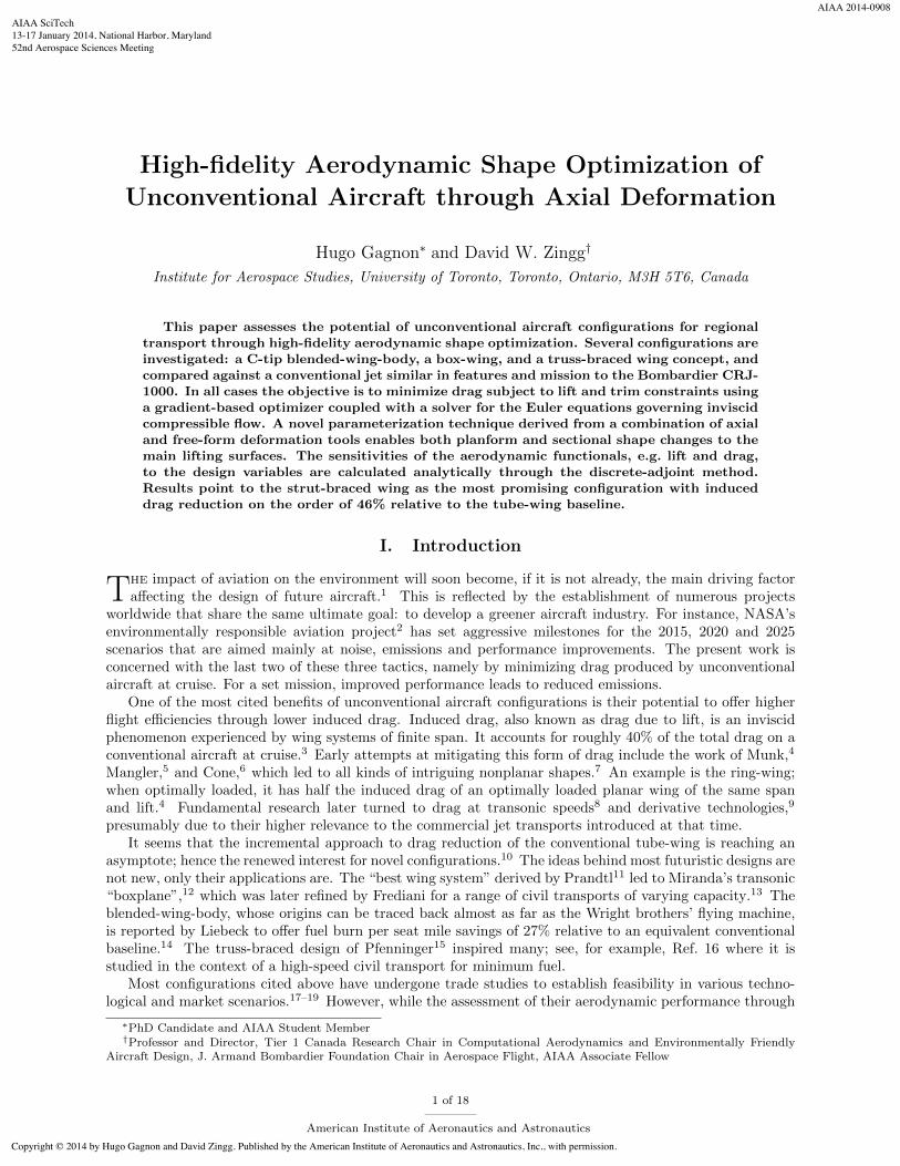
The application to wing deformation follows directly. Refer to Figure 2 where the chordwise, spanwise,and vertical directions of the wing are assumed to be oriented along the positive X, Y, and Z directions,respectively.

Let the axial curve be a NURBS curve33 defined with n control points Pi and n piecewise rational

polynomials of degree p, R(p)i (u):

A (u) =n�

i=1

R(p)i (u)Pi, 0 ≤ u ≤ 1. (1)

The basis functions are joined at non-decreasing knot locations {ui}n+p+1i=1 , where the end knot multiplicities

must equal the order of the splines in order for A(0) and A(1) to pass exactly through the end control pointsP1 and Pn, respectively.

x1

z1

y1

z2

x2y2

z3y3 x3

x4

z4y4

Z

YX

Axial curveAxial curve control pointsFFD volume control points

Figure 2: Axial-driven free-form deformation applied to ageneric wing.

The first step is to position A(u) relativeto the wing, for example at the wing’s quarter-chord curve as shown in Figure 2. Next, rela-tive to the global origin, O, a local orthonormalcoordinate system {o(u),x(u),y(u), z(u)} thatmoves along A(u) is introduced. For any givenu ∈ [0, 1], let

o(u) = A(u), y(u) =A

�(u)⊥�A�(u)⊥�

, (2)

where the prime denotes the first derivative in uand the ⊥ symbol refers to the projected vectoronto the YZ plane (the reason for this projec-tion will be clarified below). We define wingtwist to be about the axial curve, and com-pute z(u) directly from its spanwise distribu-tion. Indeed, assuming B(u) to be a vector-valued function satisfying B(u) · y(u) = 0 forall u, we have

z(u) =B(u)

�B(u)� . (3)

Finally, x(u) is simply defined asx(u) = y(u)× z(u). (4)

3 of 18


For the special case of an untwisted wing, then x(u) = X for all u (hence y(u) and z(u) appear perpendicularwhen looking in the X direction).

The next step is to enclose the wing inside a sufficiently large FFD lattice whose spanwise cross-sectionsare oriented according to the local coordinate functions described by Eqs. (2–4). Specifically, let u1, . . . , um

be the parameters associated with m such cross-sections; then the local coordinate system associated withthe first one is {o(u1),x(u1),y(u1), z(u1)}, and so forth. Also notice, in Figure 2 (where m = 4), how controlpoints pertaining to the same cross-section reside in the same plane perpendicular to the local y axis. Thisrequirement, together with the projection of y(u) in Eq. 2, is required in order to keep wing cross-sectionsfacing the flow field no matter what the orientation of A(u) becomes. Lastly, as for the degree selectionof the FFD splines, we use cubic NURBS both in the chordwise and spanwise directions, but linear in thevertical direction. This choice forces the number of control points in the vertical direction to two, and to aminimum of four in the other two directions.

Once the FFD volume is setup, and each one of its spanwise lattice cross-sections “attached” to a pointon the axial curve, the wing’s surfaces are embedded (mapped) to the FFD volume (as apposed to the axialcurve, as originally proposed by Lazarus). This is normally carried out by a Newton search procedure,and needs only be performed once. An important note here is that we embed the surfaces’ control pointsrather than their discretizations. This allows us to integrate surface and volume mesh movement tightly forincreased computational efficiency. More on this topic is given in the next section.

At this point the axial curve can be deformed, followed by the FFD lattice, and finally the embeddedwing. Manipulating the axial curve’s control points enables variations in span, sweep, and dihedral. To varytwist, chord, and sectional shape, a sequence of transformation matrices34,35 can be applied separately toeach FFD cross-section. For example, let S(Q, c, w) be a scaling operator where Q is the scaling origin, c thescaling factor, and w the scaling direction; then S(o(u1), x, z(u1)) scales an FFD control point pertainingto the first cross-section by a factor of x in the local vertical direction, thus impacting the wing’s sectionalshape within the region of influence of that control point. Because other transformations are similarly takenabout the local origins {o(ui)}mi=1, it should be clear that the position of the axial curve relative to the wingmatters; if say, twist about the trailing edge is desired then the axial curve should be positioned accordingly.

By judiciously choosing the number and placement of control points of both the axial curve and attachedFFD volume, as well as their degree, it is possible to achieve any combination of linear or nonlinear variationsin span, sweep, dihedral, twist, chord, and sectional shape. We also emphasize the fact that the sole purposeof the axial curve is to “drive” the movement of the FFD volume, and as such both entities are completelydecoupled insofar as their mathematical definitions go. This is desirable, for example, in cases where moreFFD cross-sections are required for increased local surface control but without the typical increase in numberof planform design variables.

III. Discrete Adjoint-Based Aerodynamic Optimizer

The axial deformation scheme just introduced is part of a broader ASO methodology developed by theUniversity of Toronto Computational Aerodynamics Group. The core components of the methodology arethoroughly described and verified in Ref. 36; thus only a brief summary is given here.

Following an update in the design variables, e.g. the xyz-coordinates of axial control points, wing sectionsare regenerated by updating the location of the embedded surface control points. To account for thesechanges inside the computational domain, we initially fit our multi-block grids with as many FFD volumesas there are blocksa, and we make sure that the FFD control points bordering the geometry fall exactlyon the embedded control points of the wings. This allows us to apply the equations of linear elasticityto this much coarser grid of FFD control points and to subsequently regenerate the computational meshalgebraically. This semi-algebraic method results in fast, high-quality mesh movements and is robust enoughto accommodate very large shape changes.28,36

With the computational mesh conforming to the deformed geometry, the aerodynamic functionals arethen evaluated based on the solution of the Euler governing equations. Those are discretized with second-order accurate finite-difference summation-by-parts operators.37 Simultaneous approximation terms38 areapplied to enforce boundary conditions and couple blocks, requiring only C0 continuity between matchingmesh lines at interfaces. The solution in the vicinity of shocks is stabilized by a pressure switch mechanisminvolving both second- and fourth-difference scalar dissipation. Further details regarding the flow solver are

aThis second level of FFD volumes is completely separate from those of the axial-driven FFD, see Ref. 28.

4 of 18


available in Ref. 39.We use the gradient-based optimization package SNOPT40 to find locally optimal designs. SNOPT is

based on sequential quadratic programming, where the Hessian of the Lagrangian is approximated usingthe quasi-Newton method of Broyden, Fletcher, Goldfarb, and Shanno.41 SNOPT is capable of handlingproblems with large numbers of design variables and constraints, as long as all gradient entries are provided bythe userb. For aerodynamic functionals, which depend on the flow, the gradients are calculated analyticallyby using discrete-adjoint variables.36 Other constraints, such as projected area and volume, are mostlyhand-differentiated. In all cases the sensitivity of the surface control points to the axial design variables arecomputed to machine accuracy with the complex-step method.42

IV. Applications to Unconventional Aircraft

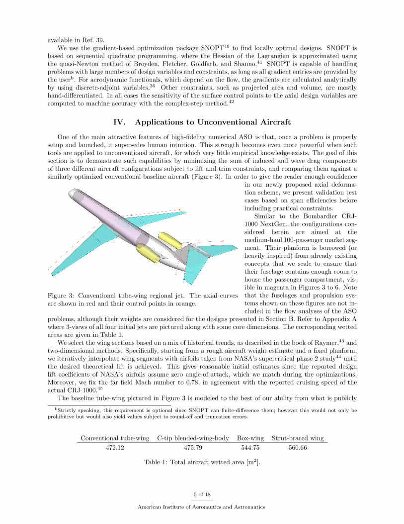
One of the main attractive features of high-fidelity numerical ASO is that, once a problem is properlysetup and launched, it supersedes human intuition. This strength becomes even more powerful when suchtools are applied to unconventional aircraft, for which very little empirical knowledge exists. The goal of thissection is to demonstrate such capabilities by minimizing the sum of induced and wave drag componentsof three different aircraft configurations subject to lift and trim constraints, and comparing them against asimilarly optimized conventional baseline aircraft (Figure 3). In order to give the reader enough confidence

Figure 3: Conventional tube-wing regional jet. The axial curvesare shown in red and their control points in orange.

in our newly proposed axial deforma-tion scheme, we present validation testcases based on span efficiencies beforeincluding practical constraints.

Similar to the Bombardier CRJ-1000 NextGen, the configurations con-sidered herein are aimed at themedium-haul 100-passenger market seg-ment. Their planform is borrowed (orheavily inspired) from already existingconcepts that we scale to ensure thattheir fuselage contains enough room tohouse the passenger compartment, vis-ible in magenta in Figures 3 to 6. Notethat the fuselages and propulsion sys-tems shown on these figures are not in-cluded in the flow analyses of the ASO

problems, although their weights are considered for the designs presented in Section B. Refer to Appendix Awhere 3-views of all four initial jets are pictured along with some core dimensions. The corresponding wettedareas are given in Table 1.

We select the wing sections based on a mix of historical trends, as described in the book of Raymer,43 andtwo-dimensional methods. Specifically, starting from a rough aircraft weight estimate and a fixed planform,we iteratively interpolate wing segments with airfoils taken from NASA’s supercritical phase 2 study44 untilthe desired theoretical lift is achieved. This gives reasonable initial estimates since the reported designlift coefficients of NASA’s airfoils assume zero angle-of-attack, which we match during the optimizations.Moreover, we fix the far field Mach number to 0.78, in agreement with the reported cruising speed of theactual CRJ-1000.45

The baseline tube-wing pictured in Figure 3 is modeled to the best of our ability from what is publicly

bStrictly speaking, this requirement is optional since SNOPT can finite-difference them; however this would not only beprohibitive but would also yield values subject to round-off and truncation errors.

Conventional tube-wing C-tip blended-wing-body Box-wing Strut-braced wing

472.12 475.79 544.75 560.66

Table 1: Total aircraft wetted area [m2].

5 of 18


available on the CRJ-1000. The pressurized cabin is designed for a 2-2 seating arrangement and long enoughto seat 104 passengers in economy class. Rather than trying to replicate the exact winglet (which is takenfrom the CRJ-900, which is itself a scaled version of the one found on the CRJ-700), we choose not to modelany on the initial geometry but, as discussed in Section B, we give the optimizer enough freedom to produceone on its own. The main wing is essentially a scaled-up version of the CRJ-700 W34 planform:46 straightleading edge swept back 30 degrees with a root plug ending at 35% span. Based on the airfoil selectiondesign process described above, we opt for the NASA SC(2)-0614, -0412, and -0410 at the root, kink, andtip sections, respectively. This choice yields satisfactory lift coefficients at the expense of small wave dragpenalties.

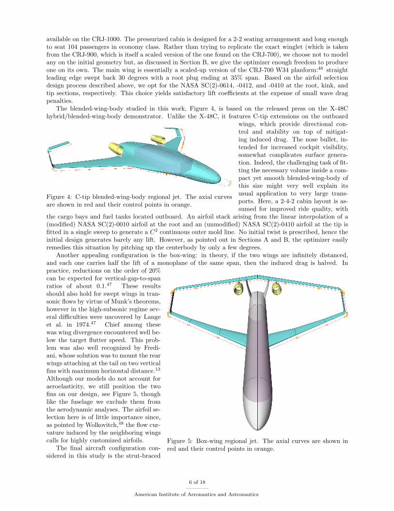
The blended-wing-body studied in this work, Figure 4, is based on the released press on the X-48Chybrid/blended-wing-body demonstrator. Unlike the X-48C, it features C-tip extensions on the outboard

Figure 4: C-tip blended-wing-body regional jet. The axial curvesare shown in red and their control points in orange.

wings, which provide directional con-trol and stability on top of mitigat-ing induced drag. The nose bullet, in-tended for increased cockpit visibility,somewhat complicates surface genera-tion. Indeed, the challenging task of fit-ting the necessary volume inside a com-pact yet smooth blended-wing-body ofthis size might very well explain itsusual application to very large trans-ports. Here, a 2-4-2 cabin layout is as-sumed for improved ride quality, with

the cargo bays and fuel tanks located outboard. An airfoil stack arising from the linear interpolation of a(modified) NASA SC(2)-0010 airfoil at the root and an (unmodified) NASA SC(2)-0410 airfoil at the tip isfitted in a single sweep to generate a C2 continuous outer mold line. No initial twist is prescribed, hence theinitial design generates barely any lift. However, as pointed out in Sections A and B, the optimizer easilyremedies this situation by pitching up the centerbody by only a few degrees.

Another appealing configuration is the box-wing: in theory, if the two wings are infinitely distanced,and each one carries half the lift of a monoplane of the same span, then the induced drag is halved. In

Figure 5: Box-wing regional jet. The axial curves are shown inred and their control points in orange.

practice, reductions on the order of 20%can be expected for vertical-gap-to-spanratios of about 0.1.47 These resultsshould also hold for swept wings in tran-sonic flows by virtue of Munk’s theorems,however in the high-subsonic regime sev-eral difficulties were uncovered by Langeet al. in 1974.47 Chief among thesewas wing divergence encountered well be-low the target flutter speed. This prob-lem was also well recognized by Fredi-ani, whose solution was to mount the rearwings attaching at the tail on two verticalfins with maximum horizontal distance.13

Although our models do not account foraeroelasticity, we still position the twofins on our design, see Figure 5, thoughlike the fuselage we exclude them fromthe aerodynamic analyses. The airfoil se-lection here is of little importance since,as pointed by Wolkovitch,48 the flow cur-vature induced by the neighboring wingscalls for highly customized airfoils.

The final aircraft configuration con-sidered in this study is the strut-braced

6 of 18


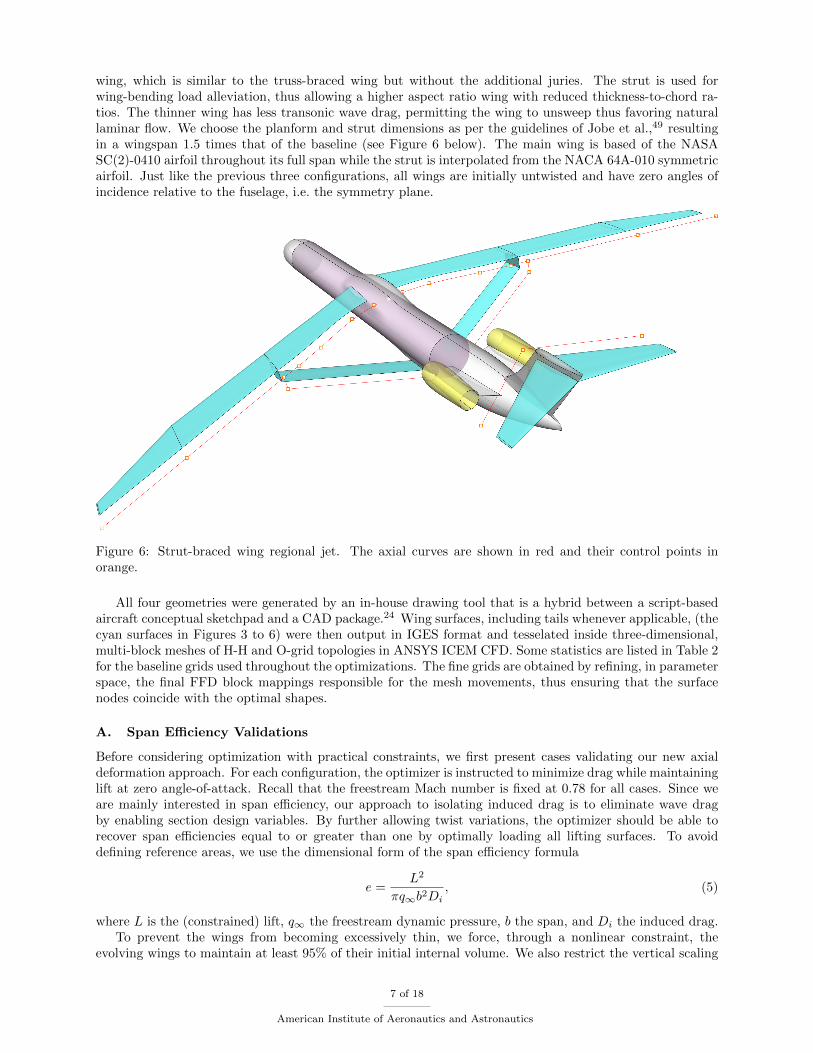
wing, which is similar to the truss-braced wing but without the additional juries. The strut is used forwing-bending load alleviation, thus allowing a higher aspect ratio wing with reduced thickness-to-chord ra-tios. The thinner wing has less transonic wave drag, permitting the wing to unsweep thus favoring naturallaminar flow. We choose the planform and strut dimensions as per the guidelines of Jobe et al.,49 resultingin a wingspan 1.5 times that of the baseline (see Figure 6 below). The main wing is based of the NASASC(2)-0410 airfoil throughout its full span while the strut is interpolated from the NACA 64A-010 symmetricairfoil. Just like the previous three configurations, all wings are initially untwisted and have zero angles ofincidence relative to the fuselage, i.e. the symmetry plane.

Figure 6: Strut-braced wing regional jet. The axial curves are shown in red and their control points inorange.

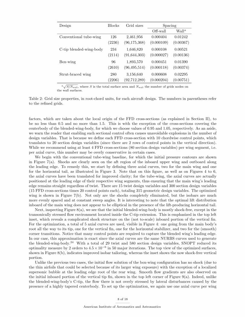
All four geometries were generated by an in-house drawing tool that is a hybrid between a script-basedaircraft conceptual sketchpad and a CAD package.24 Wing surfaces, including tails whenever applicable, (thecyan surfaces in Figures 3 to 6) were then output in IGES format and tesselated inside three-dimensional,multi-block meshes of H-H and O-grid topologies in ANSYS ICEM CFD. Some statistics are listed in Table 2for the baseline grids used throughout the optimizations. The fine grids are obtained by refining, in parameterspace, the final FFD block mappings responsible for the mesh movements, thus ensuring that the surfacenodes coincide with the optimal shapes.

A. Span Efficiency Validations

Before considering optimization with practical constraints, we first present cases validating our new axialdeformation approach. For each configuration, the optimizer is instructed to minimize drag while maintaininglift at zero angle-of-attack. Recall that the freestream Mach number is fixed at 0.78 for all cases. Since weare mainly interested in span efficiency, our approach to isolating induced drag is to eliminate wave dragby enabling section design variables. By further allowing twist variations, the optimizer should be able torecover span efficiencies equal to or greater than one by optimally loading all lifting surfaces. To avoiddefining reference areas, we use the dimensional form of the span efficiency formula

e =L2

πq∞b2Di, (5)

where L is the (constrained) lift, q∞ the freestream dynamic pressure, b the span, and Di the induced drag.To prevent the wings from becoming excessively thin, we force, through a nonlinear constraint, the

evolving wings to maintain at least 95% of their initial internal volume. We also restrict the vertical scaling

7 of 18


Design Blocks Grid sizes Spacing

Off-wall Walla

Conventional tube-wing 126 2,461,956 0.000404 0.01242

(2236) (96,175,368) (0.000109) (0.00367)

C-tip blended-wing-body 234 1,646,820 0.000108 0.00521

(2114) (91,644,303) (0.000027) (0.00136)

Box-wing 96 1,893,570 0.000451 0.01390

(2610) (96,495,514) (0.000118) (0.00374)

Strut-braced wing 280 3,156,640 0.000608 0.02295

(2206) (92,712,289) (0.000204) (0.00751)

a�

S/Nwall, where S is the total surface area and Nwall the number of grids nodes onthe wall surfaces.

Table 2: Grid size properties, in root-chord units, for each aircraft design. The numbers in parentheses referto the refined grids.

factors, which are taken about the local origin of the FFD cross-sections (as explained in Section II), tobe no less than 0.5 and no more than 1.5. This is with the exception of the cross-sections covering thecenterbody of the blended-wing-body, for which we choose values of 0.95 and 1.05, respectively. As an aside,we warn the reader that enabling such sectional control often causes unavoidable explosions in the number ofdesign variables. That is because we define each FFD cross-section with 10 chordwise control points, whichtranslates to 20 section design variables (since there are 2 rows of control points in the vertical direction).While we recommend using at least 4 FFD cross-sections (80 section design variables) per wing segment, i.e.per axial curve, this number may be overly conservative in certain cases.

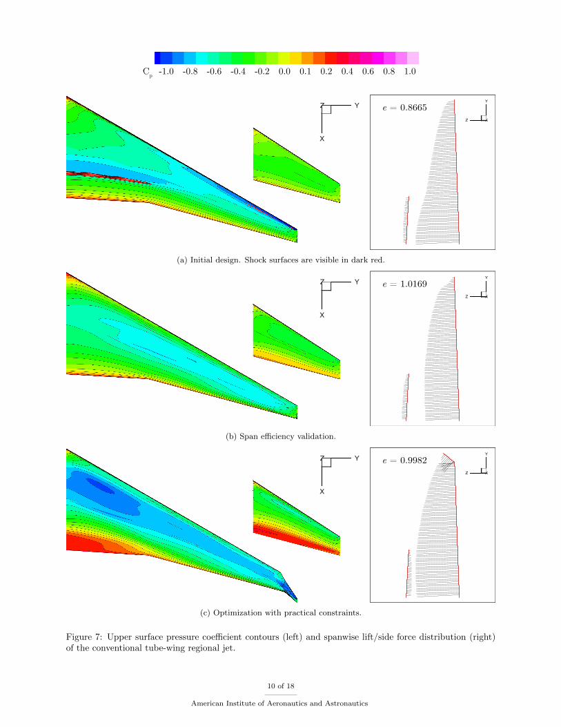
We begin with the conventional tube-wing baseline, for which the initial pressure contours are shownin Figure 7(a). Shocks are clearly seen on the aft region of the inboard upper wing and outboard alongthe leading edge. To remedy this, we start by defining three axial curves, two for the main wing and onefor the horizontal tail, as illustrated in Figure 3. Note that on this figure, as well as on Figures 4 to 6,the axial curves have been translated for improved clarity; for the tube-wing, the axial curves are actuallypositioned at the leading edge of their respective wing segments, thus ensuring that the main wing’s leadingedge remains straight regardless of twist. There are 15 twist design variables and 300 section design variables(15 FFD cross-sections times 20 control points each), totaling 315 geometric design variables. The optimizedwing is shown in Figure 7(b). Not only are the shocks completely eliminated, but the isobars are muchmore evenly spaced and at constant sweep angles. It is interesting to note that the optimal lift distributioninboard of the main wing does not appear to be elliptical in the presence of the lift-producing horizontal tail.

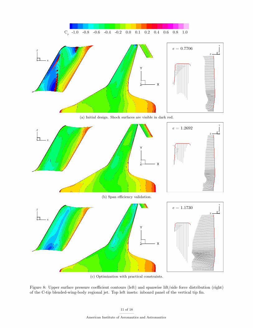
Next, inspecting Figure 8(a), we see that the initial blended-wing-body is mostly shock-free, except in thetransonically stressed flow environment located inside the C-tip extension. This is emphasized in the top leftinset, which reveals a complicated shock structure on the (not to-scale) inboard portion of the vertical fin.For the optimization, a total of 5 axial curves are used, visible in Figure 4: one going from the main body’sroot all the way to its tip, one for the vertical fin, one for the horizontal stabilizer, and two for the (smooth)corner transitions. Notice that many control points are required to capture the blended wing’s leading edge.In our case, this approximation is exact since the axial curves are the same NURBS curves used to generatethe blended-wing-body.24 With a total of 29 twist and 580 section design variables, SNOPT reduced itsoptimality measure by 2 orders to 4.5× 10−6 in 50 major iterations. The top view of the optimized surfaces,shown in Figure 8(b), indicates improved isobar tailoring, whereas the inset shows the now shock-free verticalportion.

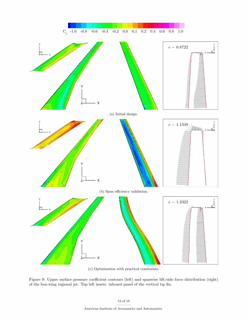
Unlike the previous two cases, the initial flow solution of the box-wing configuration has no shock (due tothe thin airfoils that could be selected because of its larger wing exposure) with the exception of a localizedsupersonic bubble at the leading edge root of the rear wing. Smooth flow gradients are also observed onthe initial inboard portion of the vertical tip fin, shown in the top left corner of Figure 9(a). Indeed, unlikethe blended-wing-body’s C-tip, the flow there is not overly stressed by lateral disturbances caused by thepresence of a highly tapered centerbody. To set up the optimization, we again use one axial curve per wing

8 of 18


segment, plus two for the corner fillets, for a total of 7 axial curves. In all, there are 30 twist and 600 sectiondesign variables. Although the optimization converged by 2 orders and reduced overall drag by roughly 30%,the resulting spanwise lift distribution (Figure 9(b), right) is surprising. The optimizer almost completelyunloaded the front wing by quite literally reversing its camber; hence, most of the lift is carried by therear wing. This setting does form a favorable induced flow field for the (normally downwashed) rear wing,however this solution does not correspond to the global optimum. Indeed, as discussed in Section B, higherspan efficiencies can be obtained when the two wings are encouraged to produce the same lift.

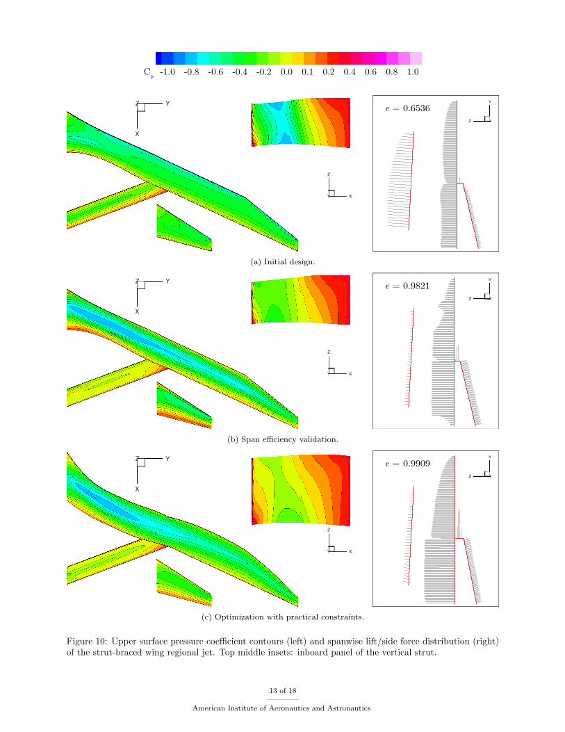
Just like the box-wing, the strut-braced wing has thin airfoil sections and as such sees no shock waves overmost of its initial surfaces. The only detected shocks are found on the outboard panel of the strut intersectingthe wing, although we choose to show the (not to-scale) inboard panel (Figure 10(a), top middle) for its moreinteresting flow patterns. Axial curves are assigned to wing segments in a similar fashion to the previousthree cases, yielding 18 twist and 520 section design variables. The strut, being purely a structural member,is not allowed to twist and has limited freedom in sectional shape changes during the optimization. Theoptimizer takes 62 design cycles (67 function and gradient evaluations) to reduce optimality by 2 orders,from 1.7× 10−2 to 1.6× 10−4. The flow on the optimized shape is remarkably well-behaved, as seen by thecontours on Figure 10(b). Notice how the suction side of the strut is now reversed.

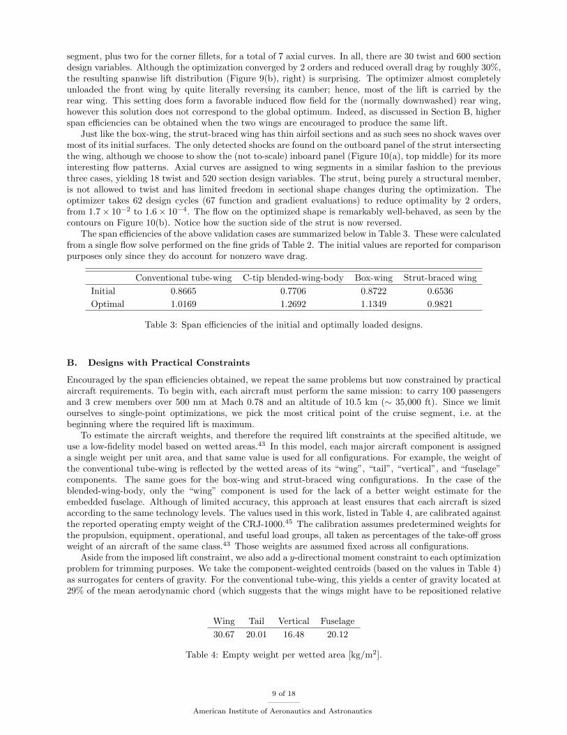
The span efficiencies of the above validation cases are summarized below in Table 3. These were calculatedfrom a single flow solve performed on the fine grids of Table 2. The initial values are reported for comparisonpurposes only since they do account for nonzero wave drag.


Initial 0.8665 0.7706 0.8722 0.6536

Optimal 1.0169 1.2692 1.1349 0.9821

Table 3: Span efficiencies of the initial and optimally loaded designs.

B. Designs with Practical Constraints

Encouraged by the span efficiencies obtained, we repeat the same problems but now constrained by practicalaircraft requirements. To begin with, each aircraft must perform the same mission: to carry 100 passengersand 3 crew members over 500 nm at Mach 0.78 and an altitude of 10.5 km (∼ 35,000 ft). Since we limitourselves to single-point optimizations, we pick the most critical point of the cruise segment, i.e. at thebeginning where the required lift is maximum.

To estimate the aircraft weights, and therefore the required lift constraints at the specified altitude, weuse a low-fidelity model based on wetted areas.43 In this model, each major aircraft component is assigneda single weight per unit area, and that same value is used for all configurations. For example, the weight ofthe conventional tube-wing is reflected by the wetted areas of its “wing”, “tail”, “vertical”, and “fuselage”components. The same goes for the box-wing and strut-braced wing configurations. In the case of theblended-wing-body, only the “wing” component is used for the lack of a better weight estimate for theembedded fuselage. Although of limited accuracy, this approach at least ensures that each aircraft is sizedaccording to the same technology levels. The values used in this work, listed in Table 4, are calibrated againstthe reported operating empty weight of the CRJ-1000.45 The calibration assumes predetermined weights forthe propulsion, equipment, operational, and useful load groups, all taken as percentages of the take-off grossweight of an aircraft of the same class.43 Those weights are assumed fixed across all configurations.

Aside from the imposed lift constraint, we also add a y-directional moment constraint to each optimizationproblem for trimming purposes. We take the component-weighted centroids (based on the values in Table 4)as surrogates for centers of gravity. For the conventional tube-wing, this yields a center of gravity located at29% of the mean aerodynamic chord (which suggests that the wings might have to be repositioned relative

Wing Tail Vertical Fuselage

30.67 20.01 16.48 20.12

Table 4: Empty weight per wetted area [kg/m2].

9 of 18


Cp -1.0 -0.8 -0.6 -0.4 -0.2 0.0 0.1 0.2 0.4 0.6 0.8 1.0

X

YZ

X

Y

Z

e = 0.8665

(a) Initial design. Shock surfaces are visible in dark red.

X

YZ

X

Y

Z

e = 1.0169

(b) Span efficiency validation.

X

YZ

X

Y

Z

e = 0.9982

(c) Optimization with practical constraints.

Figure 7: Upper surface pressure coefficient contours (left) and spanwise lift/side force distribution (right)of the conventional tube-wing regional jet.

10 of 18


Cp -1.0 -0.8 -0.6 -0.4 -0.2 0.0 0.1 0.2 0.4 0.6 0.8 1.0

X

Y

Z

Y X

Z

X

Y

Z

e = 0.7706

(a) Initial design. Shock surfaces are visible in dark red.

X

Y

Z

Y X

Z

X

Y

Z

e = 1.2692


X

Y

Z

Y X

Z

X

Y

Z

e = 1.1730


Figure 8: Upper surface pressure coefficient contours (left) and spanwise lift/side force distribution (right)of the C-tip blended-wing-body regional jet. Top left insets: inboard panel of the vertical tip fin.

11 of 18


Cp -1.0 -0.8 -0.6 -0.4 -0.2 0.0 0.1 0.2 0.4 0.6 0.8 1.0

X

Y

Z

e = 0.8722

X

Y

Z

Y X

Z

(a) Initial design.

X

Y

Z

e = 1.1349

X

Y

Z

Y X

Z


X

Y

Z

e = 1.2322

X

Y

Z

Y X

Z


Figure 9: Upper surface pressure coefficient contours (left) and spanwise lift/side force distribution (right)of the box-wing regional jet. Top left insets: inboard panel of the vertical tip fin.

12 of 18


Cp -1.0 -0.8 -0.6 -0.4 -0.2 0.0 0.1 0.2 0.4 0.6 0.8 1.0

X

Y

Z

e = 0.6536

X

YZ

Y X

Z

(a) Initial design.

X

Y

Z

e = 0.9821

X

YZ

Y X

Z


X

Y

Z

e = 0.9909

X

YZ

Y X

Z


Figure 10: Upper surface pressure coefficient contours (left) and spanwise lift/side force distribution (right)of the strut-braced wing regional jet. Top middle insets: inboard panel of the vertical strut.

13 of 18


to the fuselage, but such action was deemed unnecessary given the lack of a stability criterion in our models).The same goes for the unconventional aircraft, but, in order to account for their greater overall uncertaintyin say, wing planform, the longitudinal position of their center of gravity is considered a design variable,with a margin with respect to the centroid of plus or minus 3% of the fuselage length.

We reuse the same axial curve/FFD volume combinations as in Section A, but this time we free up some ofthe axial curves’ control points with the goal of exploring the design space of each configuration. Dependingon the configuration at hand, we try to do so in a manner that is sensible both from an aerodynamic and astructural point of view. For example, for the conventional wing only, we allow a winglet to grow (to helpit compete with the unconventional designs), but we heavily restrict the winglet’s taper (to help reduce theroot bending moment). In general, because there is no structural model involved, we allow neither wingspan nor wing sweep to vary during any of the optimizations.

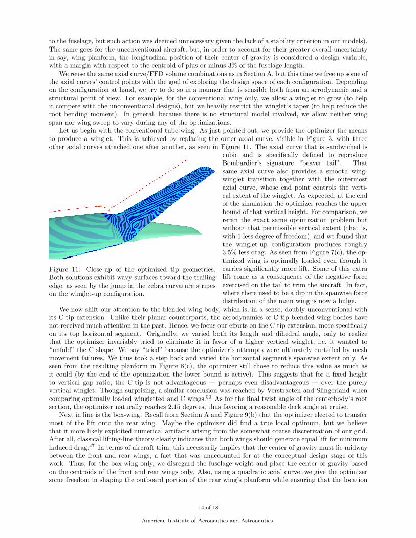
Let us begin with the conventional tube-wing. As just pointed out, we provide the optimizer the meansto produce a winglet. This is achieved by replacing the outer axial curve, visible in Figure 3, with threeother axial curves attached one after another, as seen in Figure 11. The axial curve that is sandwiched is

Figure 11: Close-up of the optimized tip geometries.Both solutions exhibit wavy surfaces toward the trailingedge, as seen by the jump in the zebra curvature stripeson the winglet-up configuration.

cubic and is specifically defined to reproduceBombardier’s signature “beaver tail”. Thatsame axial curve also provides a smooth wing-winglet transition together with the outermostaxial curve, whose end point controls the verti-cal extent of the winglet. As expected, at the endof the simulation the optimizer reaches the upperbound of that vertical height. For comparison, wereran the exact same optimization problem butwithout that permissible vertical extent (that is,with 1 less degree of freedom), and we found thatthe winglet-up configuration produces roughly3.5% less drag. As seen from Figure 7(c), the op-timized wing is optimally loaded even though itcarries significantly more lift. Some of this extralift come as a consequence of the negative forceexercised on the tail to trim the aircraft. In fact,where there used to be a dip in the spanwise forcedistribution of the main wing is now a bulge.

We now shift our attention to the blended-wing-body, which is, in a sense, doubly unconventional withits C-tip extension. Unlike their planar counterparts, the aerodynamics of C-tip blended-wing-bodies havenot received much attention in the past. Hence, we focus our efforts on the C-tip extension, more specificallyon its top horizontal segment. Originally, we varied both its length and dihedral angle, only to realizethat the optimizer invariably tried to eliminate it in favor of a higher vertical winglet, i.e. it wanted to“unfold” the C shape. We say “tried” because the optimizer’s attempts were ultimately curtailed by meshmovement failures. We thus took a step back and varied the horizontal segment’s spanwise extent only. Asseen from the resulting planform in Figure 8(c), the optimizer still chose to reduce this value as much asit could (by the end of the optimization the lower bound is active). This suggests that for a fixed heightto vertical gap ratio, the C-tip is not advantageous — perhaps even disadvantageous — over the purelyvertical winglet. Though surprising, a similar conclusion was reached by Verstraeten and Slingerland whencomparing optimally loaded wingletted and C wings.50 As for the final twist angle of the centerbody’s rootsection, the optimizer naturally reaches 2.15 degrees, thus favoring a reasonable deck angle at cruise.

Next in line is the box-wing. Recall from Section A and Figure 9(b) that the optimizer elected to transfermost of the lift onto the rear wing. Maybe the optimizer did find a true local optimum, but we believethat it more likely exploited numerical artifacts arising from the somewhat coarse discretization of our grid.After all, classical lifting-line theory clearly indicates that both wings should generate equal lift for minimuminduced drag.47 In terms of aircraft trim, this necessarily implies that the center of gravity must lie midwaybetween the front and rear wings, a fact that was unaccounted for at the conceptual design stage of thiswork. Thus, for the box-wing only, we disregard the fuselage weight and place the center of gravity basedon the centroids of the front and rear wings only. Also, using a quadratic axial curve, we give the optimizersome freedom in shaping the outboard portion of the rear wing’s planform while ensuring that the location

14 of 18


where the vertical fin intersects remains unchanged. Finally, linear taper variations are activated on all wingsegments, thus giving the optimizer the opportunity to redistribute internal volume between the front andrear wings. As portrayed in Figure 9(c), the optimal solution exhibits almost equally loaded wings. Indeed,the spanwise lift distribution closely resembles the one found by Prandtl in 1924: elliptical on both wingsand joined at the tip by a butterfly-shaped side-force distribution.11

The final case considered is the strut-braced wing, for which we further relax the axial curves’ rangeof potential deformation. First, similar to the box-wing design, we activate the chordwise scaling variables(taper) along the main wing, but this time we allow nonlinear changes. Because the axial curves are positionedon the wing’s trailing edge, the latter will remain straight as taper is varied. Second, the first four axialcurve’s points controlling the inboard wing segment (of which the very first appears inside the fuselage inFigure 6) are free to move in the chordwise direction by plus or minus 0.2 root-chord units. Hence, for thisregion only the curvature of the trailing edge can potentially vary. Finally, the height of the vertical strutsegment is also subjected to change by plus or minus 0.1 root-chord units. At the end of the optimization,the optimizer reaches the lower bound of that last design variable, thus maximizing the vertical gap betweenthe wing and the horizontal strut segment. This relieves the flow passing through the wing-strut opening.Also, visible in Figure 10(c) and of higher interest is the final planform. The initial kink at about 80% spanappears to disappear, blended by a smooth bird-like leading edge. The inboard wing is also curved, but insuch a way to maximize the root sweep angle so to delay isobar unsweeping at the symmetry plane.

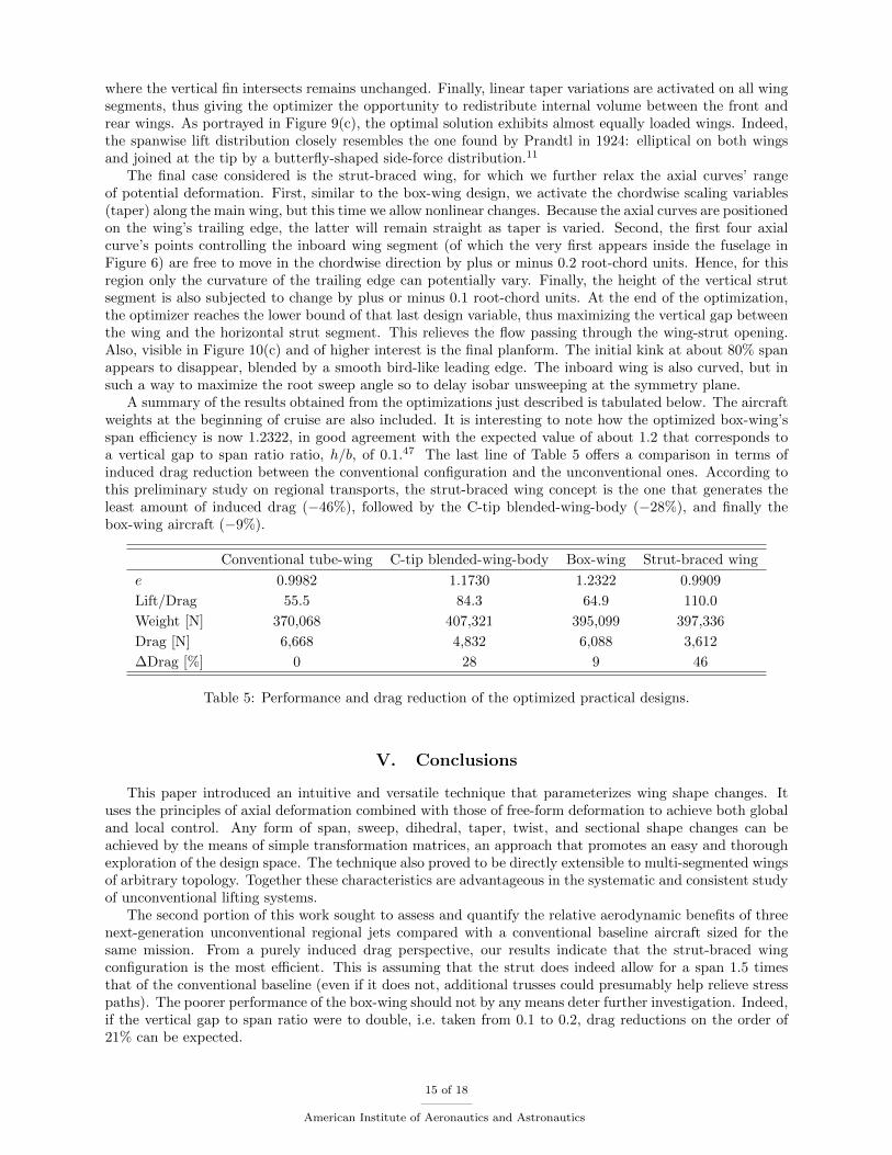
A summary of the results obtained from the optimizations just described is tabulated below. The aircraftweights at the beginning of cruise are also included. It is interesting to note how the optimized box-wing’sspan efficiency is now 1.2322, in good agreement with the expected value of about 1.2 that corresponds toa vertical gap to span ratio ratio, h/b, of 0.1.47 The last line of Table 5 offers a comparison in terms ofinduced drag reduction between the conventional configuration and the unconventional ones. According tothis preliminary study on regional transports, the strut-braced wing concept is the one that generates theleast amount of induced drag (−46%), followed by the C-tip blended-wing-body (−28%), and finally thebox-wing aircraft (−9%).


e 0.9982 1.1730 1.2322 0.9909

Lift/Drag 55.5 84.3 64.9 110.0

Weight [N] 370,068 407,321 395,099 397,336

Drag [N] 6,668 4,832 6,088 3,612

∆Drag [%] 0 28 9 46

Table 5: Performance and drag reduction of the optimized practical designs.

V. Conclusions

This paper introduced an intuitive and versatile technique that parameterizes wing shape changes. Ituses the principles of axial deformation combined with those of free-form deformation to achieve both globaland local control. Any form of span, sweep, dihedral, taper, twist, and sectional shape changes can beachieved by the means of simple transformation matrices, an approach that promotes an easy and thoroughexploration of the design space. The technique also proved to be directly extensible to multi-segmented wingsof arbitrary topology. Together these characteristics are advantageous in the systematic and consistent studyof unconventional lifting systems.

The second portion of this work sought to assess and quantify the relative aerodynamic benefits of threenext-generation unconventional regional jets compared with a conventional baseline aircraft sized for thesame mission. From a purely induced drag perspective, our results indicate that the strut-braced wingconfiguration is the most efficient. This is assuming that the strut does indeed allow for a span 1.5 timesthat of the conventional baseline (even if it does not, additional trusses could presumably help relieve stresspaths). The poorer performance of the box-wing should not by any means deter further investigation. Indeed,if the vertical gap to span ratio were to double, i.e. taken from 0.1 to 0.2, drag reductions on the order of21% can be expected.

15 of 18


Two secondary outcomes of the optimizations are worth reiterating. The first is that a box-wing isoptimally loaded only when the front and rear wings carry the same amount of lift, which entails that thecenter of gravity should be halfway between the two wings. This observation could only be made possiblewith sufficiently fine mesh spacings, fine enough to capture the many subtleties present in the induced flowfield generated by the staggered wings. The second point is that a C wing does not appear to offer anydrag benefit over a vertical winglet of the same height to span ratio. Either this trend represents a realphenomenon, or, similar to the box-wing, our grid was simply too coarse to capture the real physics. Morework is needed to elucidate this dilemma.

This paper only marks the beginning in assessing the real potential of unconventional aircraft for com-mercial aviation. It remains to be determined whether viscous effects negate savings in induced drag. Forinstance, a 2011 NASA contractor report reveals that the only way to achieve a 30% reduction in inducedand parasitic drag (along with a 30% improvement in vehicle weight and engine fuel consumption) for the2035 timeframe is to substantially reduce wetted area, such as could be achieved by a tailless airliner.51 Thisreport goes to show the unusually strong coupling between the many disciplines involved in the design ofunconventional aircraft; hence future work will not only address viscous effects but also include structuralmodels culminating in high-fidelity multi-point aerostructural optimizations.

Acknowledgments

We are thankful for the financial support provided by the Ontario Graduate Scholarship (OGS) in con-junction with the University of Toronto. Computations were performed on the gpc supercomputer at theSciNet HPC Consortium.

References

1Green, J. E., “Civil aviation and the environment - the next frontier for the aerodynamicist,” The Aeronautical Journal ,Vol. 110, No. 1110, August 2006, pp. 469–486.

2Collier, F., “Overview of NASA’s Environmentally Responsible Aviation (ERA) Project,” 48th AIAA Aerospace Sciences

Meeting, Orlando, Florida, January 2010.3Kroo, I. M., “Drag due to lift: concepts for prediction and reduction,” Annual Review of Fluid Mechanics, Vol. 33, No. 1,

January 2001, pp. 587–617.4Munk, M. M., “The Minimum Induced Drag of Aerofoils,” Tech. Rep. 121, National Advisory Committee for Aeronautics,

1921.5Mangler, W., “The Lift Distribution of Wings with End Plates,” Tech. Rep. 856, National Advisory Committee for

Aeronautics, 1938.6Cone, C. D. J., “The Theory of Induced Lift and Minimum Induced Drag of Nonplanar Lifting Systems,” Tech. Rep.

139, National Aeronautics and Space Administration, 1962.7Kroo, I. M., “Nonplanar Wing Concepts for Increased Aircraft Efficiency,” VKI Lecture Series on Innovation Configu-

rations and Advanced Concepts for Future Civil Aircraft , Rhode-St-Genese, Belgium, June 2005.8Whitcomb, R., “Research on Methods for Reducing the Aerodynamic Drag at Transonic Speeds,” Inaugural Eastman

Jacobs Lecture, NASA Langley Research Center, November 1994.9Bushnell, D., “Aircraft drag reduction — a review,” Proceedings of the Institution of Mechanical Engineers, Part G:

Journal of Aerospace Engineering, Vol. 217, No. 1, January 2003, pp. 1–18.10Torenbeek, E. and Deconinck, H., editors, Innovative configurations and advanced concepts for future civil transport

aircraft . von Karman Institute for Fluid Dynamics, June 2005.11Prandtl, L., “Induced Drag of Multiplanes,” Tech. Rep. 182, National Advisory Committee for Aeronautics, 1924.12Miranda, L. R., “Boxplane Configuration — Conceptual Analysis and Initial Experimental Verification,” Tech. Rep.

25180, Lockheed-California Company, 1972.13Frediani, A., “The Prandtl wing,” Innovative configurations and advanced concepts for future civil transport aircraft ,

edited by E. Torenbeek and H. Deconinck, von Karman Institute for Fluid Dynamics, June 5–10 2005.14Liebeck, R. H., “Design of the Blended Wing Body Subsonic Transport,” Journal of Aircraft , Vol. 41, No. 1, January-

February 2004, pp. 10–25.15Pfenninger, W., “Laminar Flow Control Laminarization,” Tech. Rep. 654, Advisory Group for Aerospace Research and

Development, 1976.16Gur, O., Schetz, J. A., and Mason, W. H., “Aerodynamic Considerations in the Design of Truss-Braced-Wing Aircraft,”

Journal of Aircraft , Vol. 48, No. 3, May-June 2011, pp. 919–939.17Lange, R. H., “Review of Unconventional Aircraft Design Concepts,” Journal of Aircraft , Vol. 25, No. 5, May 1988,

pp. 385–392.18Schmitt, D., “Challenges for unconventional transport aircraft configurations,” Air & Space Europe, Vol. 3, No. 3–4,

2001, pp. 67–72.

16 of 18


19Kehayas, N., “Aeronautical technology for future subsonic civil transport aircraft,” Aircraft Engineering and Aerospace

Technology: An International Journal (January 2007), Vol. 79, No. 6, January 2007, pp. 600–610.20Qin, N., Vavalle, A., Le Moigne, A., Laban, M., Hackett, K., and Weinerfelt, P., “Aerodynamic considerations of blended

wing body aircraft,” Progress in Aerospace Sciences, Vol. 40, No. 6, August 2004, pp. 321–343.21Qin, N., Vavalle, A., and Le Moigne, A., “Spanwise Lift Distribution for Blended Wing Body Aircraft,” Journal of

Aircraft , Vol. 42, No. 2, March-April 2005, pp. 356–365.22Lyu, Z. and Martins, J. R. R. A., “Aerodynamic Shape Optimization of a Blended-Wing-Body Aircraft,” 51st AIAA

Aerospace Sciences Meeting, AIAA Paper 2013-0283, Grapevine, Texas, January 2013.23Reist, T. A. and Zingg, D. W., “Aerodynamic Shape Optimization of a Blended-Wing-Body Regional Transport for a

Short Range Mission,” 21st AIAA Computational Fluid Dynamics Conference, AIAA Paper 2012-2414, San Diego, California,June 2013.

24Gagnon, H. and Zingg, D. W., “Geometry Generation of Complex Unconventional Aircraft with Application to High-Fidelity Aerodynamic Shape Optimization,” 21st AIAA Computational Fluid Dynamics Conference, AIAA Paper 2013-2850,San Diego, California, June 2013.

25Ning, S. A. and Kroo, I., “Tip Extensions, Winglets, and C-wings: Conceptual Design and Optimization,” 28th AIAA

Applied Aerodynamics Conference, AIAA Paper 2008-7052, Honolulu, Hawaii, August 2008.26Jansen, P. W., Perez, R. E., and Martins, J. R. R. A., “Aerostructural Optimization of Nonplanar Lifting Surfaces,”

Journal of Aircraft , Vol. 47, No. 5, 2010, pp. 1490–1503.27Anderson, G. R., Aftosmis, M. J., and Nemec, M., “Parametric Deformation of Discrete Geometry for Aerodynamic

Shape Design,” 50th AIAA Aerospace Sciences Meeting, AIAA Paper 2012-0965, Nashville, Tennessee, January 2012.28Gagnon, H. and Zingg, D. W., “Two-Level Free-Form Deformation for High-Fidelity Aerodynamic Shape Optimization,”

14th AIAA/ISSMO Multidisciplinary Analysis and Optimization Conference, AIAA Paper 2012-5447, Indianapolis, Indiana,September 2012.

29Fudge, D., Zingg, D. W., and Haimes, R., “A CAD-Free and a CAD-Based Geometry Control System for AerodynamicShape Optimization,” 43rd AIAA Aerospace Sciences Meeting, AIAA Paper 2005-0451, Reno, Nevada, January 2005.

30Sederberg, T. W. and Parry, S. R., “Free-Form Deformation of Solid Geometric Models,” Proceedings of the 13th Annual

Conference on Computer Graphics and Interactive Techniques, Dallas, Texas, August 1986.31Lazarus, F., Coquillart, S., and Jancene, P., “Axial deformations: an intuitive deformation technique,” Computer-Aided

Design, Vol. 26, No. 8, 1994, pp. 607–613.32Gain, J. and Bechmann, D., “A Survey of Spatial Deformation from a User-Centered Perspective,” ACM Transactions

of Graphics, Vol. 27, No. 4, 2008, pp. 107:1–107:21.33Piegl, L. A., “On NURBS: a survey,” Computer Graphics and Applications, Vol. 11, No. 1, 1991, pp. 55–71.34Goldman, R., Matrices and Transformations, Graphics Gems I, Academic Press, 1990.35Goldman, R., More Matrices and Transformations: Shear and Pseudo-Perspective, Graphics Gems II, Academic Press,

1991.36Hicken, J. E. and Zingg, D. W., “Aerodynamic Optimization Algorithm with Integrated Geometry Parameterization and

Mesh Movement,” AIAA Journal , Vol. 48, No. 2, February 2010, pp. 400–413.37Strand, B., “Summation by parts for finite difference approximations for d/dx,” Journal of Computational Physics,

Vol. 110, No. 1, January 1994, pp. 47–67.38Carpenter, M. H., Gottlieb, D., and Abarbanel, S., “Time-stable boundary conditions for finite-difference schemes solving

hyperbolic systems: methodology and application to high-order compact schemes,” Journal of Computational Physics, Vol. 111,No. 2, April 1994, pp. 220–236.

39Hicken, J. E. and Zingg, D. W., “Parallel Newton-Krylov Solver for the Euler Equations Discretized Using Simultaneous-Approximation Terms,” AIAA Journal , Vol. 46, No. 11, November 2008, pp. 2273–2786.

40Gill, P. E., Murray, W., and Saunders, M. A., “SNOPT: An SQP Algorithm for Large-Scale Constrained Optimization,”SIAM Review , Vol. 47, No. 1, 2005, pp. 99–131.

41Nocedal, J. and Wright, S. J., Numerical Optimization, Springer, 2nd ed., 2006.42Squire, W. and Trapp, G., “Using Complex Variables to Estimate Derivatives of Real Functions,” SIAM Review , Vol. 40,

No. 1, March 1998, pp. 110–112.43Raymer, D. P., Aircraft Design: A Conceptual Approach, American Institute of Aeronautics and Astronautics, Blacks-

burg, Virginia, 4th ed., 2006.44Harris, C. D., “NASA Supercritical Airfoils,” Tech. Rep. Paper 2969, National Aeronautics and Space Administration,

Hampton, Virginia, 1990.45Bombardier Inc., “Results speak,” [http://www.crjnextgen.com, accessed 09/12/13].46Kafyeke, F., Pepin, F., and Kho, C., “Development of High-Lift Systems for the Bombardier CRJ-700,” 23rd International

Congress of the Aeronautical Sciences, Toronto, Ontario, September 2002.47Lange, R. H., Cahill, J. F., Bradley, E. S., Eudaily, R. R., Jenness, C. M., and MacWilkinson, D. G., “Feasibility Study

of the Transonic Biplane Concept for Transport Aircraft Application,” Tech. Rep. 132462, National Aeronautics and SpaceAdministration, 1974.

48Wolkovitch, J., “The Joined Wing: An Overview,” Journal of Aircraft , Vol. 23, No. 3, March 1986, pp. 161–178.49Jobe, C. E., Kulfan, R. M., and Vachal, J. D., “Wing Planforms for Large Military Transports,” Journal of Aircraft ,

Vol. 16, No. 7, July 1979, pp. 425–432.50Verstraeten, J. G. and Slingerland, R., “Drag Characteristics for Optimally Span-Loaded Planar, Wingletted, and C

Wings,” Journal of Aircraft , Vol. 46, No. 3, May-June 2009, pp. 962–971.51Raymer, D. P., Wilson, J., Douglas Perkins, H., Rizzi, A., Zhang, M., and Ramirez Puentes, A., “Advanced Technology

Subsonic Transport Study,” Tech. Rep. 217130, National Aeronautics and Space Administration, Cleveland, Ohio, 2011.

17 of 18


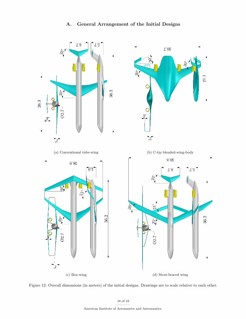
A. General Arrangement of the Initial Designs

(a) Conventional tube-wing (b) C-tip blended-wing-body

(c) Box-wing (d) Strut-braced wing

Figure 12: Overall dimensions (in meters) of the initial designs. Drawings are to scale relative to each other.

18 of 18
