Habit persistence, consumption based asset pricing,and time-varying expected returns
Stig Vinther MøllerDepartment of Business Studies
Aarhus School of Business, University of Aarhus
September 2008

Table of contents
� Acknowledgements
� Summary
� Dansk resumé (Danish summary)
� Chapter 1: An iterated GMM procedure for estimating the Campbell-Cochranehabit formation model, with an application to Danish stock and bond returns
� Chapter 2: Habit persistence: Explaining cross-sectional variation in returns andtime-varying expected returns
� Chapter 3: Habit formation, surplus consumption and return predictability: Inter-national evidence
� Chapter 4: Consumption growth and time-varying expected stock returns
1

AcknowledgementsFirst and foremost, I would like to express my sincere gratitude to my thesis advisor
Tom Engsted for providing guidance and numerous insightful comments and suggestionsthroughout my Ph.D. studies. Two of the chapters in this thesis are co-authored withTom Engsted, and I am grateful for having had the opportunity to work with him. Ialso thank Stuart Hyde who I worked with in the spring of 2007, while I was visitingManchester Business School on a Marie Curie Fellowship.
During my Ph.D. studies, I enjoyed very much the friendly atmosphere at the De-partment of Business Studies, and I thank my colleagues for generating a pleasant andmotivating research environment. I also thank the Department of Business Studies forgenerous �nancial support that gave me the opportunity to attend several courses, work-shops and conferences.
I would also like to take this opportunity to thank the members of the assessmentcommittee � Björn Hansson, Jesper Rangvid, and Esben Høg (chairman) � for theiruseful and insightful suggestions.
Last, but not least, a special thank you to my girlfriend Carina for your invaluablemoral support and much needed patience during the entire process of writing this thesis.
2
SummaryWithin the consumption based asset pricing framework, the habit persistence model of
Campbell and Cochrane (1999) model has become one of the leading models in explainingasset pricing behavior. Campbell and Cochrane show that their model explains a numberof stylized facts on the US stock market, including pro-cyclical stock prices, time-varyingcounter-cyclical expected returns on stocks, and it has the ability to explain the equitypremium puzzle without facing a risk-free rate puzzle. Campbell and Cochrane andsubsequent applications of their model only rely on calibration and simulation exercisesand do not engage in formal econometric estimation and testing of the model. Given thefact that the Campbell-Cochrane model seems to work so well in several dimensions, itis also of great relevance to estimate and test the model econometrically.
In the �rst chapter "An iterated GMM procedure for estimating the Campbell-Cochranehabit formation model, with an application to Danish stock and bond returns" (joint workwith Tom Engsted), we perform formal econometric estimation and testing of the modelusing Danish stock and bond returns. To our knowledge, there have been no formaleconometric studies of the Campbell-Cochrane model on data from other countries thanthe US. Our paper is the �rst attempt to �ll this gap. Denmark is interesting becausehistorically over a long period of time the average return on Danish stocks has not beennearly as high as in the US and most other countries, and at the same time the returnon Danish bonds has been somewhat higher than in other countries, see e.g. Engstedand Tanggaard (1999), Engsted (2002), and Dimson et al. (2002). Thus, the Danishequity premium is not nearly as high as in most other countries, and might not even beregarded a puzzle. The results we obtain using our GMM procedure on Danish assetmarket returns do not in general support the conclusions from the US studies. Althoughthere is some evidence of time-varying counter-cyclical risk aversion in recent years, theCampbell-Cochrane model does not produce lower pricing errors or more plausible para-meter values than the benchmark CRRA model.1
The second chapter "Habit persistence: Explaining cross-sectional variation in re-turns and time-varying expected returns" estimates and tests the Campbell-Cochranemodel along both cross-sectional and time-series dimensions of the US stock market.The model is estimated in a cross-sectional setting using the 25 Fama and French valueand size portfolios, which has not been tried previously, cf. Cochrane (2007). The cross-sectional estimation documents that the model is able to explain the size premium, butfails to explain the value premium. Besides cross-sectional variation in returns, I examinewhether the model is able to account for variation in expected returns over time. Con-sistently with the model, I �nd that low surplus consumption ratios in recession timespredict high future stock returns. Thus, the model captures time-varying counter-cyclicalexpected returns on stocks.2
In the third chapter "Habit formation, surplus consumption and return predictability:International evidence" (joint work with Tom Engsted and Stuart Hyde), we present
1The paper is forthcoming in the International Journal of Finance and Economics.2The paper has been invited for third resubmission to the Journal of Empirical Finance.
3
further international evidence on the relative performance of the Campbell-Cochranemodel and the benchmark CRRA model. There seems to be quite large cross-countrydi¤erences in the ability of the Campbell-Cochrane model to explain stock and bondreturn movements over time, but for the majority of the countries in our sample, themodel gets empirical support in a variety of di¤erent dimensions. The model generatescounter-cyclical time-varying relative risk aversion, and in contrast to the benchmarkCRRA model, the Campbell-Cochrane model has the important ability to escape therisk-free rate puzzle. Moreover, we �nd that the surplus consumption ratio is a strongpredictive variable of future stock and bond returns. Since a common limitation toexisting predictive variables is that they only contain information about either futurestock returns or future bond returns, the ability of the surplus consumption ratio tocapture predictive patterns in both stock and bond markets is particularly interesting.
The fourth chapter "Consumption growth and time-varying expected returns" exam-ines the ability of the consumption growth rate to predict future stock returns. Previousstudies show that the consumption growth rate has no predictive power for future stockreturns. However, I �nd that the consumption growth rate based upon fourth quarterdata is a strong predictive variable of future stock returns. The fourth quarter con-sumption growth rate explains a substantial amount of the variation in 1-year aheadstock returns and is a better predictive variable than traditional benchmark predictivevariables such as the price-dividend ratio [Campbell and Shiller (1988) and Fama andFrench (1988, 1989)] and performs marginally better than new predictive variables suchas the consumption-wealth ratio [Lettau and Ludvigson (2001)] in predicting future stockreturns. Interestingly, when the consumption growth rate is measured based upon otherquarters, the predictive power breaks down. This striking evidence is consistent with theinsight of Jagannathan and Wang (2007) that investors tend to review their consumptionand investments plans during the end of each calendar year, and at possibly random timesin between. Importantly, the fourth quarter consumption growth rate is an almost i.i.d.process, which eliminates potential concerns about �nding spurious evidence of returnpredictability, cf. Stambaugh (1999).3
3The paper is published in Finance Research Letters, 2008 volume 5, pages 129-136.
4

Dansk resumé (Danish summary)Indenfor det forbrugsbaserede asset pricing framework er Campbell og Cochrane�s
(1999) habit persistence model blevet en af de førende modeller i at forklare prisfastsæt-telsen på aktiver. Campbell og Cochrane viser, at deres model forklarer en række stilis-erede facts på det amerikanske aktiemarked inklusiv pro-cykliske aktiekurser, tidsvari-erende kontra-cykliske forventede afkast på aktier, og modellen har evnen til at forklareequity premium puzzlet uden at blive konfronteret med et risk-free rate puzzle. Camp-bell og Cochrane og efterfølgende applikationer af deres model beror udelukkende påkalibrering og simulering og anvender ikke formel økonometrisk estimering og testningaf modellen. Givet det faktum, at Campbell-Cochrane modellen synes at fungere sågodt i �ere dimensioner, er det også af væsentlig relevans at estimere og teste modellenøkonometrisk.
I det første kapitel "An iterated GMM procedure for estimating the Campbell-Cochranehabit formation model, with an application to Danish stock and bond returns" (fælles ar-bejde med Tom Engsted) foretager vi formel økonometrisk estimering og testning af mod-ellen ved brug af danske aktie- og obligationsafkast. Ud fra vores kendskab har der ikkeværet formelle økonometriske studier af Campbell-Cochrane modellen på data fra andrelande end USA. Vores artikel er det første forsøg på at udfylde dette hul i litteraturen.Danmark er interessant, fordi historisk set over en lang tidsperiode har det gennemsnitligeafkast på danske aktier ikke været nært så højt som i USA og de �este andre lande, ogsamtidigt har afkastet på danske obligationer været noget højere end i andre lande, seeksempelvis Engsted and Tanggaard (1999), Engsted (2002), og Dimson mf. (2002).Dermed er den danske risikopræmie ikke nær så høj som i de �este andre lande og ansesmuligvis ikke engang for værende et puzzle. De resultater vi opnår med vores GMM pro-cedure anvendt på danske aktie- og obligationsafkast støtter generelt ikke konklusionernefra de amerikanske studier. Selvom der i nogen grad er beviser på tidsvarierende kontra-cyklisk risikoaversion i de seneste år, producerer Campbell-Cochrane modellen ikke lavereprisfejl eller mere plausible parameterværdier end benchmark CRRA modellen.4
Det andet kapital "Habit persistence: Explaining cross-sectional variation in returnsand time-varying expected returns" estimerer og tester Campbell-Cochrane modellen påbåde tværsnits- og tidsseriedimensioner af det amerikanske aktiemarked. Modellen es-timeres i et tværsnit setup ved at bruge de 25 Fama og French value og size porteføljer,hvilket ikke har været forsøgt tidligere, jævnfør Cochrane (2007). Tværsnitsestimerin-gen dokumenterer, at modellen er i stand til at forklare the size premium, men kanikke forklare the value premium. Foruden tværsnitsvariation i aktieafkast undersøgerjeg, hvorvidt modellen er i stand til at forklare variation i forventede afkast over tid. Ioverensstemmelse med modellen �nder jeg, at lave overskudsforbrugsratioer i recession-stider forudsiger høje fremtidige aktieafkast. Dermed opfanger modellen tidsvarierendekontra-cykliske afkast på aktier.5
I det tredje kapitel "Habit formation, surplus consumption and return predictabil-
4Artiklen udkommer i International Journal of Finance and Economics.5Artiklen er blevet inviteret til tredje genindsendelse til Journal of Empirical Finance.
5

ity: International evidence" (fælles arbejde med Tom Engsted og Stuart Hyde) præsen-terer vi yderligere international dokumentation af den relative performance af Campbell-Cochrane modellen og benchmark CRRA modellen. På tværs af lande synes der at væreganske store forskelle i Campbell-Cochrane modellens evne til at forklare bevægelser iaktie- og obligationsafkast over tid. For hovedparten af landene i vores stikprøve op-når modellen dog empirisk støtte i en lang række forskellige dimensioner. Modellengenererer kontra-cyklisk tidsvarierende relativ risikoaversion, og i modsætning til bench-mark CRRA modellen, har Campbell-Cochrane modellen den vigtige evne til at slippefri af risk-free rate puzzlet. Ydermere �nder vi, at overskudsforbrugsratioen er en stærkforecastvariabel af fremtidige aktie- og obligationsafkast. Da en fælles begrænsning foreksisterende forecastvariable er, at de udelukkende indeholder information om enten frem-tidige aktieafkast eller fremtidige obligationsafkast, er overskudsforbrugsratioens evne tilat opfange forudsigelige mønstre i både aktie- og obligationsmarkedet særligt interessant.
Det fjerde kapitel "Consumption growth and time-varying expected returns" under-søger forbrugsvækstens evne til at forudsige fremtidige aktieafkast. Tidligere under-søgelser viser, at forbrugsvæksten ikke har forecaststyrke for fremtidige aktieafkast. Imi-dlertid �nder jeg, at forbrugsvæksten baseret på fjerde kvartalsdata er en stærk forecast-variabel af fremtidige aktieafkast. Forbrugsvæksten i fjerde kvartal forklarer en væsentligdel af variationen i aktieafkast 1 år frem i tiden og er en bedre forecastvariabel end tra-ditionelle benchmark forecastvariable såsom pris-dividende ratioen [Campbell og Shiller(1988) og Fama og French (1988, 1989)] og klarer sig marginalt bedre end nye fore-castvariable såsom forbrug-formue ratioen [Lettau og Ludvigson (2001)] i at forudsigefremtidige aktieafkast. Når forbrugsvæksten måles baseret på andre kvartaler, bryderforecaststyrken sammen. Dette iøjnefaldende resultat er konsistent med Jagannathan ogWang�s (2007) indsigt, at investorerne har en tendens til at revurdere deres forbrug- oginvesteringsplaner ved afslutningen af hvert kalenderår og på mulige tilfældige tidspunk-ter ind imellem. Hvad der er nok så vigtigt, er forbrugsvæksten i fjerde kvartal tæt påat være en i.i.d. proces, hvilket eliminerer potentielle bekymringer om at �nde falskebeviser på afkastforudsigelighed, jf. Stambaugh (1999).6
6Artiklen er publiceret i Finance Research Letters, 2008 volume 5, side 129-136.
6
References
[1] Campbell, J.Y., Shiller, R., 1988. The dividend-price ratio and expectations of futuredividends and discount factors. Review of Financial Studies 1, 195-208.
[2] Campbell, J.Y., Cochrane, J.H., 1999. By force of habit: A consumption basedexplanation of aggregate stock market behavior. Journal of Political Economy 107,205-251.
[3] Cochrane, J.H., 2007. Financial markets and the real economy. In: Mehra, R., Theequity premium, North Holland Handbook of Finance Series, North Holland, Ams-terdam.
[4] Dimson, E., Marsh, P., Staunton, M., 2002. Triumph of the optimists: 101 Years ofglobal investment returns. Princeton University Press.
[5] Engsted, T. (2002). Measures of �t for rational expectations models. Journal ofEconomic Surveys 16, 301-355.
[6] Engsted, T., Tanggaard, C., 1999. The equity premium on Danish stocks (in Danish).Journal of the Danish Economic Association (Nationaløkonomisk Tidsskrift) 137,164-177.
[7] Fama, E.F., French, K.R., 1988. Dividend yields and expected stock returns. Journalof Financial Economics 22, 3-25.
[8] Fama, E.F., French, K.R., 1989. Business conditions and expected returns on stocksand bonds. Journal of Financial Economics 25, 23-49.
[9] Jagannathan, R., Wang, Y., 2007. Lazy investors, discretionary consumption, andthe cross-section of stock returns, Journal of Finance 62, 1623-1661.
[10] Lettau, M., Ludvigson, S., 2001. Consumption, aggregate wealth and expected re-turns. Journal of Finance 55, 815-849.
[11] Stambaugh, R.F., 1999. Predictive regressions. Journal of Financial Economics 54,375-421.
7

Chapter 1
An iterated GMM procedure for estimating the Campbell-Cochrane habitformation model, with an application to Danish stock and bond returns
An iterated GMM procedure for estimating theCampbell-Cochrane habit formation model, with anapplication to Danish stock and bond returns�
Tom Engstedy Stig Vinther Møllerz
Forthcoming in the International Journal of Finance and Economics
Abstract
We suggest an iterated GMM approach to estimate and test the consumption basedhabit persistence model of Campbell and Cochrane (1999), and we apply the ap-proach on annual and quarterly Danish stock and bond returns. For compara-tive purposes we also estimate and test the standard CRRA model. In addition,we compare the pricing errors of the di¤erent models using Hansen and Jagan-nathan�s (1997) speci�cation error measure. The main result is that for Denmarkthe Campbell-Cochrane model does not seem to perform markedly better than theCRRA model. For the long annual sample period covering more than 80 years thereis absolutely no evidence of superior performance of the Campbell-Cochrane model.For the shorter and more recent quarterly data over a 20-30 year period, there issome evidence of counter-cyclical time-variation in the degree of risk-aversion, inaccordance with the Campbell-Cochrane model, but the model does not producelower pricing errors or more plausible parameter estimates than the CRRA model.
Keywords: Consumption-based model, habit persistence, GMM, pricing error.
JEL codes: C32, G12
�This paper is a substantially revised and updated version of an earlier working paper from 2005by Engsted, Møller and Tuong, "Habit persistence and asset pricing: Evidence from Denmark". Wegratefully acknowledge comments and suggestions from Stuart Hyde, an anonymous referee and seminarparticipants at the University of Aarhus. We also acknowledge support from CREATES (Center forResearch in Econometric Analysis of Time Series), funded by the Danish National Research Foundation.
yCREATES, School of Economics and Management, University of Aarhus, Building 1322, DK-8000Aarhuc C., Denmark. E-mail: [email protected].
zAarhus School of Business, University of Aarhus, Fuglesangs Allé 4, DK-8210 Aarhus V., Denmark,and CREATES. E-mail: [email protected].
1

1 Introduction
Since Mehra and Prescott�s (1985) seminal study, explaining the observed high equitypremium within the consumption based asset pricing framework has occupied a largenumber of researchers in �nance and macroeconomics. Despite an intense research e¤ort,still no consensus has emerged as to why stocks have given such a high average returncompared to bonds. At �rst sight the natural response to the equity premium puzzleis to dismiss the consumption based framework altogether. However, as emphasized byCochrane (2005), within the rational equilibrium paradigm of �nance, there is really noalternative to the consumption based model, since other models are not alternatives to� but special cases of � the consumption based model. Thus, despite its poor empiricalperformance, the consumption based framework continues to dominate studies of theequity premium on the aggregate stock market.
In a recent paper Chen and Ludvigson (2006) argue that within the equilibrium con-sumption based framework, habit formation models are the most promising and successfulin describing aggregate stock market behaviour. The most prominent habit model is theone developed by Campbell and Cochrane (1999). In this model people slowly develophabits for a high or low consumption level, such that risk-aversion becomes time-varyingand counter-cyclical. The model is able to explain the high US equity premium and anumber of other stylized facts for the US stock market. A special feature of the modelis that the average risk-aversion over time is quite high, but the risk-free rate is low andstable. Thus, the model solves the equity premium puzzle by high risk-aversion, butwithout facing a risk-free rate puzzle.
Campbell and Cochrane (1999) themselves, and most subsequent applications of theirmodel, do not estimate and test the model econometrically. Instead they calibrate themodel parameters to match the historical risk-free rate and Sharpe ratio, and then sim-ulate a chosen set of moments which are informally compared to those based on actualhistorical data. Only a few papers engage in formal econometric estimation and testingof the model. Tallarini and Zhang (2005) use an E¢ cient Method of Moments techniqueto estimate and test the model on US data. They statistically reject the model and �ndthat it has strongly counterfactual implications for the risk-free interest rate, althoughthey also �nd that the model performs well in other dimensions. Fillat and Garduno(2005) and Garcia et al. (2005) use an iterated Generalized Method of Moments ap-proach to estimate and test the model on US data. Fillat and Garduno strongly rejectthe model by Hansen�s (1982) J -test. On the other hand Garcia et al. do not reject themodel at conventional signi�cance levels. However, Garcia et al. face the problem thattheir iterated GMM approach does not lead to convergence with positive values of therisk-aversion parameter. Finally, Møller (2008) estimates the model by GMM in a cross-sectional setting using the Fama-French 25 value and size portfolios. He �nds supportfor the model although it has di¢ culties in explaining the value premium.
To our knowledge, there have been no formal econometric studies of the Campbell-Cochrane model on data from other countries than the US. Our paper is the �rst attempt
2
to �ll this gap.1 We examine the Campbell-Cochrane model�s ability to explain Danishstock and bond returns. Denmark is interesting because historically over a long periodof time the average return on Danish stocks has not been nearly as high as in the USand most other countries, and at the same time the return on Danish bonds has beensomewhat higher than in other countries, see e.g. Engsted and Tanggaard (1999), Engsted(2002), and Dimson et al. (2002). Thus, the Danish equity premium is not nearly ashigh as in most other countries, and might not even be regarded a puzzle.
On annual Danish data for the period 1922-2004 and quarterly data for the period1977-2006 we estimate and test both the standard model based on constant relativerisk-aversion (CRRA) and the Campbell-Cochrane model based on habit formation. Webasically follow the iterated GMM approach set out in Garcia et al. (2005). However, incontrast to Garcia et al., � who estimate the model parameters in two successive steps� we do a joint GMM estimation of all parameters, thereby properly taking into accountsampling error on all parameter estimates. We also compute Hansen and Jagannathan�s(1997) speci�cation error measure based on the second moment matrix of returns asweighting matrix. This measure has an intuitively appealing percentage pricing errorinterpretation, and it allows for direct comparison of the magnitude of pricing errorsacross models.
Our main �ndings are as follows. First, neither the CRRA model nor the Campbell-Cochrane model are statistically rejected by Hansen�s J -test, and pricing errors are of thesame magnitude for both models. Second, both models imply high risk-aversion and alow and plausible value for the real risk-free rate. Third, in most cases the CRRA modelproduces plausible values for the time discount factor while the Campbell-Cochrane modeldelivers implausibly low values for this parameter. These results are quite robust acrossdi¤erent data sets and instrument sets. However, when it comes to the variation overtime in the degree of relative risk-aversion in the Campbell-Cochrane model, there issome di¤erence between the long annual data set and the shorter quarterly data sets.In the annual data there is no visible counter-cyclical movement in risk-aversion, whilein the quarterly data there is some evidence of counter-cyclical variation over time inaccordance with the Campbell-Cochrane model.
The rest of the paper is organized as follows. The next section brie�y presents theconsumption-based models. Section 3 explains the iterated GMM approach used toestimate the models. Section 4 presents the empirical results based on Danish data.Finally, section 5 o¤ers some concluding remarks.
1Hyde and Sherif (2005), Hyde et al. (2005), and Li and Zhong (2005) examine the Campbell-Cochrane model using international data, but with the calibrated parameter values from the original USstudy by Campbell and Cochrane. In Engsted et al. (2008) we apply the iterated GMM approach fromthe present paper to estimate and test the Campbell-Cochrane model using an international post WorldWar II annual dataset.
3

2 The consumption based models
In this section we start by describing the standard CRRA utility version of the consump-tion based model. Since this version of the model is well-known and familiar to mostreaders, the description will be very brief. Then we give a more detailed description ofthe Campbell-Cochrane habit based model.
2.1 The CRRA utility model
Standard asset pricing theory implies that the price of an asset at time t, Pt, is determinedby the expected future asset payo¤, Yt+1, multiplied by the stochastic discount factor,Mt+1: Pt = Et(Mt+1Yt+1). The payo¤ is given as prices plus dividends, Yt+1 = Pt+1 +Dt+1, and the stochastic discount factor depends on the underlying asset pricing model.In consumption based models Mt+1 is the intertemporal marginal rate of substitution
in consumption. With power utility (constant relative risk-aversion), U(Ct) =C1� t �11� ,
where � 0 is the degree of relative risk-aversion, the stochastic discount factor becomesMt+1 = �
�Ct+1Ct
�� , where � = (1 + tp)�1 and tp is the rate of time-preference. De�ning
the gross return as Rt+1 =Pt+1+Dt+1
Pt, the asset pricing relationship can be stated as:
0 = Et
"�
�Ct+1Ct
�� Rt+1 � 1
#: (1)
Equation (1) captures the basic idea that risk-adjusted equilibrium returns are unpre-dictable. In the consumption based model, risk-adjustment takes place by multiplying theraw return with the intertemporal marginal rate of substitution in consumption. Risk-averse consumers want to smooth consumption over time, and for that purpose they use(dis)investments in the asset, thereby making a direct connection between consumptiongrowth and the asset return. The correlation between consumption growth and returnsthen becomes crucial for the equilibrium expected return. From (1) expected returns aregiven as:
Et [Rt+1] =
1� Covt�Rt+1; �
�Ct+1Ct
�� �Et
���Ct+1Ct
�� � : (2)
The higher the correlation between consumption growth and returns (the lower the cor-relation between the stochastic discount factor and returns), the higher will be expectedequilibrium return (ceteris paribus), because the higher the correlation, the less able theasset will be in helping to smooth consumption over time, which means that the assetwill be considered riskier and thereby demand a higher return.
Equation (1) lends itself directly to empirical estimation and testing within the GMMframework, c.f. section 3. Empirically the consumption based power utility model has run
4

into trouble because consumption growth and stock returns are not su¢ ciently positivelycorrelated to explain the historically observed high return on common stocks, unless thedegree of risk-aversion is extremely high. The basic problem is that unless is veryhigh, the variability of the intertemporal marginal rate of substitution cannot match thevariability of stock returns. Perhaps people are highly risk-averse, but then the powerutility model faces another problem, namely that with a high , the risk-free rate impliedby the model becomes implausibly high. For the risk-free rate the covariance with thestochastic discount factor is zero, thus from (2):
Rf;t+1 =1
Et
���Ct+1Ct
�� � : (3)
Thus, within the standard CRRA utility framework, the equity premium puzzlecannot be solved without running into a risk-free rate puzzle. This has led to the devel-opment of alternative utility models with a higher volatility of the stochastic discountfactor, and with plausible implications for the risk-free rate. The habit persistence modeldescribed in the next subsection is one such model.
2.2 The Campbell-Cochrane model
Habit formation models di¤er from the standard power utility model by letting the utilityfunction be time-nonseparable in the sense that the utility at time t depends not onlyon consumption at time t, but also on previous periods consumption. The basic ideais that people get used to a certain standard of living and thereby the utility of someconsumption level at time t will be higher (lower) if previous periods consumption waslow (high) than if previous periods consumption was high (low).
Habit formation can be modelled in a number of di¤erent ways. In the Campbell-Cochrane model utility is speci�ed as
U(Ct; Xt) =(Ct �Xt)
1� � 11� ; Ct > Xt (4)
whereXt is an external habit level that depends on previous periods consumption. De�nethe surplus consumption ratio as St = Ct�Xt
Ct. Then the stochastic discount factor can be
stated as Mt+1 = ��St+1St
Ct+1Ct
�� and the pricing equation becomes
0 = Et
"�
�St+1St
Ct+1Ct
�� Rt+1 � 1
#: (5)
Compared to the standard power utility model in (1), the Campbell-Cochrane modelimplies a stochastic discount factor that not only depends on consumption growth butalso on growth in the surplus consumption ratio. In this model relative risk-aversion is
5

no longer measured by but as St. This shows that relative risk-aversion is time-varying
and counter-cyclical: when consumption is high relative to habit, relative risk-aversionis low and expected returns are low. By contrast, when consumption is low and close tohabit, relative risk-aversion is high leading to high expected returns. Basically the modelexplains time-varying and counter-cyclical ex ante returns (which implies pro-cyclicalstock prices) as a result of time-varying and counter-cyclical risk-aversion of people.From (5) expected returns are given as:
Et [Rt+1] =
1� Covt�Rt+1; �
�St+1St
Ct+1Ct
�� �Et
���St+1St
Ct+1Ct
�� � : (6)
A crucial aspect in operationalizing the model is the modelling of the risk-free rate.Campbell and Cochrane specify the model in such a way that the risk-free rate is constantand low by construction. First, assume that consumption is lognormally distributed suchthat consumption growth is normally distributed and iid :
�ct+1 = g + vt+1; vt+1 � niid(0; �2v) (7)
where ct � log(Ct). g is the mean consumption growth rate. Next, specify the log surplusconsumption ratio st = log(St) as a stationary �rst-order autoregressive process
st+1 = (1� �)s+ �st + �(st)vt+1; (8)
where 0 < � < 1; s is the steady state level of st, and �(st) is the sensitivity functionto be speci�ed below. Note that shocks to consumption growth are modelled to have adirect impact on the surplus consumption level, and for � close to one, habit respondsslowly to these shocks.
The sensitivity function �(st) is speci�ed as follows:
�(st) =
�1S
p1� 2(st � s)� 1 if st � smax0 else
�(9)
where
S =
s�2v
1� �; smax � s+1
2(1� S2); s = log(S):
Specifying �(st) in this way implies the following equation for the log risk-free rate:
rf;t+1 = � log(�) + g � 2�2v2
�1
S
�2: (10)
As seen, no time-dependent variables appear in (10), thus the risk-free rate is constantover time. Economically this property of the model is obtained by letting the e¤ects ofintertemporal substitution and precautionary saving � which have opposite e¤ects onthe risk-free rate � cancel each other out, see Campbell and Cochrane (1999) for details.
6
Campbell and Cochrane calibrate their model with parameters chosen to match postwar US data: mean real consumption growth rate (g), mean real risk-free rate (rf),volatility (�v), etc. Then, based on the calibrated model, simulated time-series for re-turns, price-dividend ratios, etc., are generated and their properties are compared tothe properties of the actually observed post war data. In the present paper we insteadestimate the model parameters in a GMM framework. The next section describes how.
3 GMM estimation of the models
The GMM technique developed by Hansen (1982) estimates the model parameters basedon the orthogonality conditions implied by the model. Let the asset pricing equationbe 0 = Et [Mt+1(�)Rt+1 � 1], where Mt+1 is the stochastic discount factor, Rt+1 is avector of asset returns, and the vector � contains the model parameters. In the presentcontext this equation corresponds to either (1) or (5) with � = (� )0. De�ne a vector ofinstrumental variables, Zt, observable at time t. Then the asset pricing equation impliesthe following orthogonality conditions E [(Mt+1(�)Rt+1 � 1) Zt] = 0. GMM estimates� by making the sample counterpart to these orthogonality conditions as close to zero aspossible, by minimizing a quadratic form of the sample orthogonality conditions basedon a chosen weighting matrix. De�ne gT (�) = 1
T
PTt=1(Mt+1(�)Rt+1 � 1) Zt as the
sample orthogonality conditions based on T observations. Then the parameter vector �is estimated by minimizing
gT (�)0WgT (�); (11)
where W is the weighting matrix. The statistically optimal (most e¢ cient) weightingmatrix is obtained as the inverse of the covariance matrix of the sample orthogonalityconditions. Other weighting matrices can be chosen, however, and often a �xed andmodel-independent weighting matrix (the identity matrix, for example) is used in orderto make it possible to compare the magnitude of estimated pricing errors across di¤erentmodels. Such a comparison cannot be done if the statistically optimal weighting matrixis used because this matrix is model-dependent.
GMM estimation of the standard CRRA utility model (1) is straightforward. How-ever, estimation of the Campbell-Cochrane model, equation (5), is complicated by thefact that the surplus consumption ratio, St, is not observable in the same way as returns,Rt, and consumption, Ct, are directly observable. Garcia et al. (2005) suggest to gener-ate a process for st by initially estimating the parameters �, g and �2v , and setting tosome initial value, which then gives s, from which st can be constructed using (8) and astarting value for st at t = 0. Garcia et al. set s0 = s. Having obtained a series for thesurplus consumption ratio, GMM can be applied directly. Since the surplus consumptionratio depends on , however, the resulting GMM estimate of may not correspond tothe value initially imposed in generating st. Therefore, Garcia et al. iterate over byestimating the model in each iteration using GMM with the statistically optimal weight-ing matrix. Unfortunately, this procedure does not lead to convergence with a positivevalue of in their application. Instead they do a grid search that implies an estimated
7
value of close but not identical to the initially picked value.
Our procedure di¤ers from Garcia et al.�s in the following way: They estimate �,g and �2v separately in an initial step. Then, given these parameter estimates, theyestimate � and using GMM. Instead we do a joint GMM estimation of all parametersand, hence, take into account sampling error on all parameters. We report results fordi¤erent instrument sets. However, in order to economize on the number of orthogonalityconditions, we �x the instrument set to contain just a constant for the estimation of gand �2v , and a constant and lagged log price-dividend ratio for the estimation of �.Moreover, following Cochrane�s (2005) suggestion, we use the identity matrix as weightingmatrix across all GMM estimations. Thereby we attach equal weight to each asset inthe estimation.2 The use of the identity matrix has the further advantage that in ourapplication it leads to convergence with positive values of the risk-aversion parameter, incontrast to the case where we use the statistically optimal weighting matrix (Garcia etal. (2005) also face convergence problems, which might be due to their exclusive use ofthe statistically optimal weighting matrix). Thus, we restrict attention to the case withW = I.
The details of our estimation procedure are as follows. The moment conditions usedin our estimation procedure are:
0 = E
"(�
�St+1St
Ct+1Ct
�� Rt+1 � 1) Zt
#; (12)
0 = E [�ct+1 � g] ; (13)
0 = E�(�ct+1 � g)2 � �2v
�; (14)
0 = E�(pdt � �� �pdt�1) (1 pdt�1)
0� : (15)
Based on the asset equation in (5), we form the moment conditions in (12). In order toestimate the parameters �, g and �2v , the GMM estimation of the Campbell-Cochranemodel requires additional moment conditions. Given the random walk model of con-sumption in (7), we estimate g and �2v based on the moment conditions in (13) and (14).Following Campbell and Cochrane (1999) and Garcia et al. (2005), we estimate � as the�rst-order autocorrelation parameter for the log price-dividend ratio using the momentconditions in (15). This is feasible since in the Campbell-Cochrane model the surplusconsumption ratio is the only state variable, whereby the log price-dividend ratio, pdt,will inherit its dynamic properties from the log surplus consumption ratio, st.
As starting values in the GMM iterations we use OLS estimates of g, �2v , and �, and
we choose an initial value of = 1 to obtain S =q
�2v 1�� and set st = s at t = 0. From the
chosen parameter values, we obtain the st process recursively. Given st, St is obtainedas exp (st). Using this St process and with the identity matrix as weighting matrix, wejointly estimate the moment conditions (12) to (15), which gives GMM estimates of allmodel parameters �, , �, g, and �2v . The parameter estimates are used to generate a newSt process and we repeat this procedure until convergence of all estimated parameters.
2We use a GMM programme written in MatLab. The programme is available upon request.
8
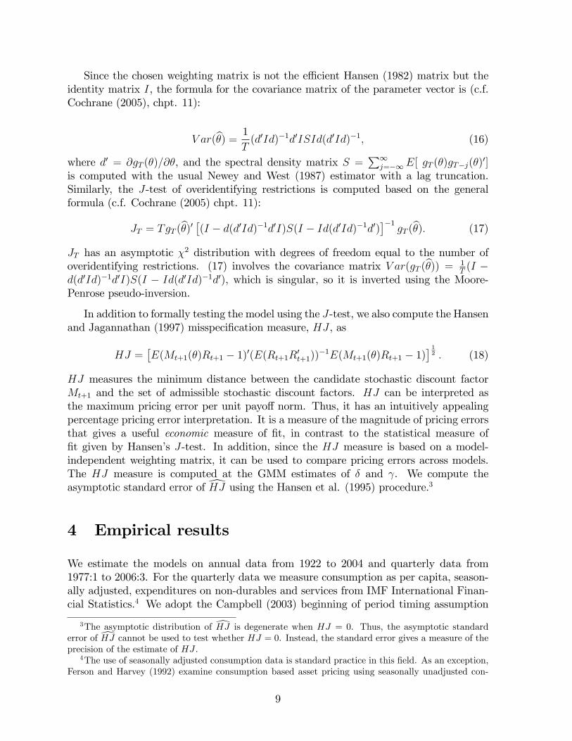
Since the chosen weighting matrix is not the e¢ cient Hansen (1982) matrix but theidentity matrix I, the formula for the covariance matrix of the parameter vector is (c.f.Cochrane (2005), chpt. 11):
V ar(b�) = 1
T(d0Id)�1d0ISId(d0Id)�1; (16)
where d0 = @gT (�)=@�, and the spectral density matrix S =P1
j=�1E[ gT (�)gT�j(�)0]
is computed with the usual Newey and West (1987) estimator with a lag truncation.Similarly, the J-test of overidentifying restrictions is computed based on the generalformula (c.f. Cochrane (2005) chpt. 11):
JT = TgT (b�)0 �(I � d(d0Id)�1d0I)S(I � Id(d0Id)�1d0)��1 gT (b�): (17)
JT has an asymptotic �2 distribution with degrees of freedom equal to the number ofoveridentifying restrictions. (17) involves the covariance matrix V ar(gT (b�)) = 1
T(I �
d(d0Id)�1d0I)S(I � Id(d0Id)�1d0), which is singular, so it is inverted using the Moore-Penrose pseudo-inversion.
In addition to formally testing the model using the J-test, we also compute the Hansenand Jagannathan (1997) misspeci�cation measure, HJ , as
HJ =�E(Mt+1(�)Rt+1 � 1)0(E(Rt+1R0t+1))�1E(Mt+1(�)Rt+1 � 1)
� 12 : (18)
HJ measures the minimum distance between the candidate stochastic discount factorMt+1 and the set of admissible stochastic discount factors. HJ can be interpreted asthe maximum pricing error per unit payo¤ norm. Thus, it has an intuitively appealingpercentage pricing error interpretation. It is a measure of the magnitude of pricing errorsthat gives a useful economic measure of �t, in contrast to the statistical measure of�t given by Hansen�s J-test. In addition, since the HJ measure is based on a model-independent weighting matrix, it can be used to compare pricing errors across models.The HJ measure is computed at the GMM estimates of � and . We compute theasymptotic standard error ofdHJ using the Hansen et al. (1995) procedure.34 Empirical results
We estimate the models on annual data from 1922 to 2004 and quarterly data from1977:1 to 2006:3. For the quarterly data we measure consumption as per capita, season-ally adjusted, expenditures on non-durables and services from IMF International Finan-cial Statistics.4 We adopt the Campbell (2003) beginning of period timing assumption
3The asymptotic distribution of dHJ is degenerate when HJ = 0. Thus, the asymptotic standarderror of dHJ cannot be used to test whether HJ = 0. Instead, the standard error gives a measure of theprecision of the estimate of HJ .
4The use of seasonally adjusted consumption data is standard practice in this �eld. As an exception,Ferson and Harvey (1992) examine consumption based asset pricing using seasonally unadjusted con-
9
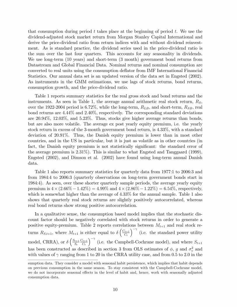
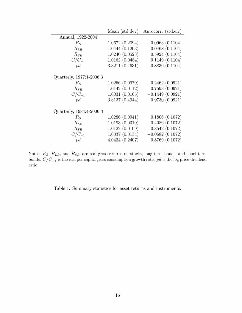
that consumption during period t takes place at the beginning of period t. We use thedividend-adjusted stock market return from Morgan Stanley Capital International andderive the price-dividend ratio from return indices with and without dividend reinvest-ment. As is standard practice, the dividend series used in the price-dividend ratio isthe sum over the last four quarters. This accounts for any seasonality in dividends.We use long-term (10 years) and short-term (3 month) government bond returns fromDatastream and Global Financial Data. Nominal returns and nominal consumption areconverted to real units using the consumption de�ator from IMF International FinancialStatistics. Our annual data set is an updated version of the data set in Engsted (2002).As instruments in the GMM estimations, we use lags of stock returns, bond returns,consumption growth, and the price-dividend ratio.
Table 1 reports summary statistics for the real gross stock and bond returns and theinstruments. As seen in Table 1, the average annual arithmetic real stock return, RS,over the 1922-2004 period is 6.72%, while the long-term, RLB, and short-term, RSB, realbond returns are 4.44% and 2.40%, respectively. The corresponding standard deviationsare 20.94%, 12.03%, and 5.23%. Thus, stocks give higher average returns than bonds,but are also more volatile. The average ex post yearly equity premium, i.e. the yearlystock return in excess of the 3-month government bond return, is 4.33%, with a standarddeviation of 20.91%. Thus, the Danish equity premium is lower than in most othercountries, and in the US in particular, but it is just as volatile as in other countries (infact, the Danish equity premium is not statistically signi�cant: the standard error ofthe average premium is 2.31%). This is similar to what Engsted and Tanggaard (1999),Engsted (2002), and Dimson et al. (2002) have found using long-term annual Danishdata.
Table 1 also reports summary statistics for quarterly data from 1977:1 to 2006:3 andfrom 1984:4 to 2006:3 (quarterly observations on long-term government bonds start in1984:4). As seen, over these shorter quarterly sample periods, the average yearly equitypremium is 4� (2:66%�1:42%) = 4:99% and 4� (2:86%�1:22%) = 6:54%, respectively,which is somewhat higher than the average of 4.33% for the annual sample. Table 1 alsoshows that quarterly real stock returns are slightly positively autocorrelated, whereasreal bond returns show strong positive autocorrelation.
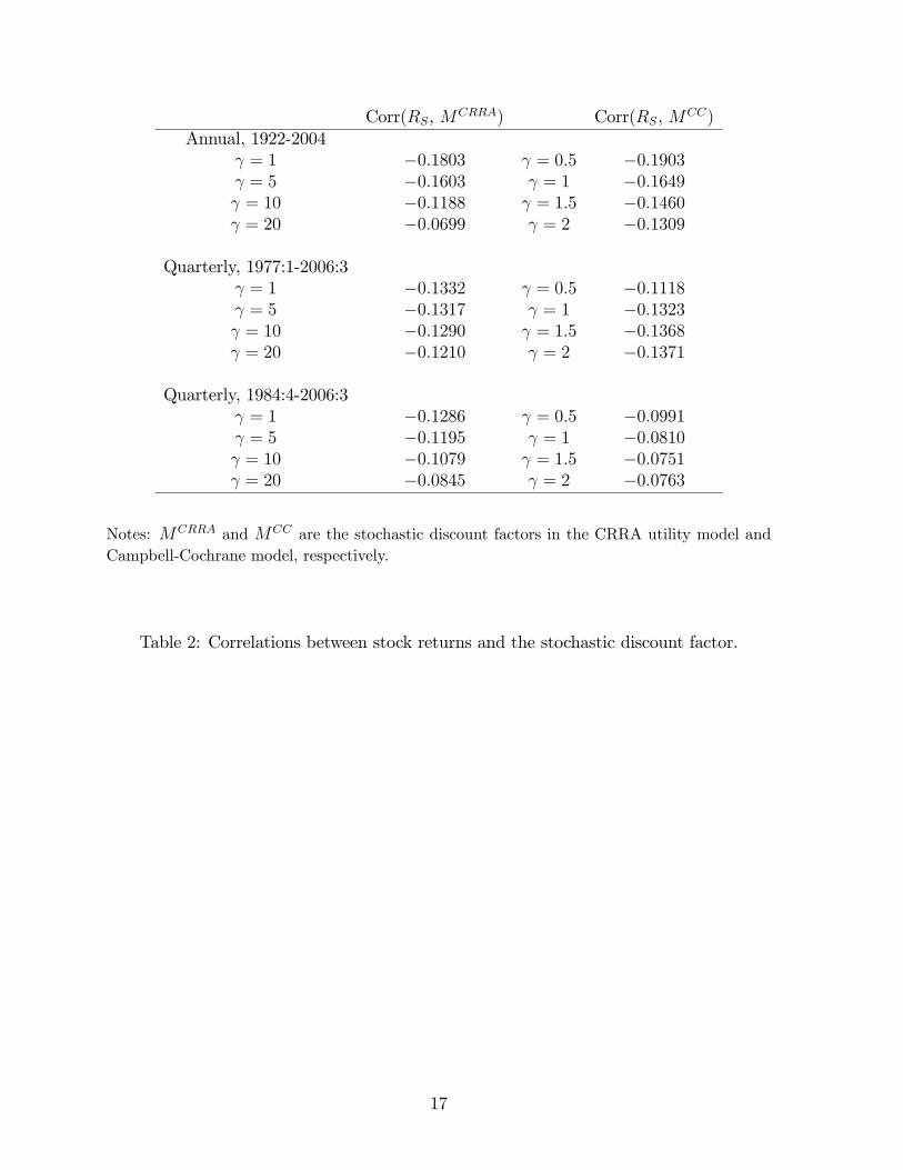
In a qualitative sense, the consumption based model implies that the stochastic dis-count factor should be negatively correlated with stock returns in order to generate apositive equity-premium. Table 2 reports correlations between Mt+1 and real stock re-
turns RS;t+1, where Mt+1 is either equal to ��Ct+1Ct
�� (i.e. the standard power utility
model, CRRA), or ��St+1St
Ct+1Ct
�� (i.e. the Campbell-Cochrane model), and where St+1
has been constructed as described in section 3 from OLS estimates of �, g and �2v andwith values of ranging from 1 to 20 in the CRRA utility case, and from 0.5 to 2.0 in the
sumption data. They consider a model with seasonal habit persistence, which implies that habit dependson previous consumption in the same season. To stay consistent with the Campbell-Cochrane model,we do not incorporate seasonal e¤ects in the level of habit and, hence, work with seasonally adjustedconsumption data.
10

Campbell-Cochrane case corresponding to values of relative risk-aversion =St rangingfrom 10 to 40, which is consistent with the GMM estimates reported below. For bothmodels � and across the di¤erent values for risk-aversion � stock returns are negativelycorrelated with the stochastic discount factor in both the annual and quarterly datasets. However, all correlations are close to zero, so although in a qualitative sense this isconsistent with the basic consumption-based framework, the evidence does not stronglysupport it and certainly does not allow us to discriminate between the standard CRRAutility model and the Campbell-Cochrane model.
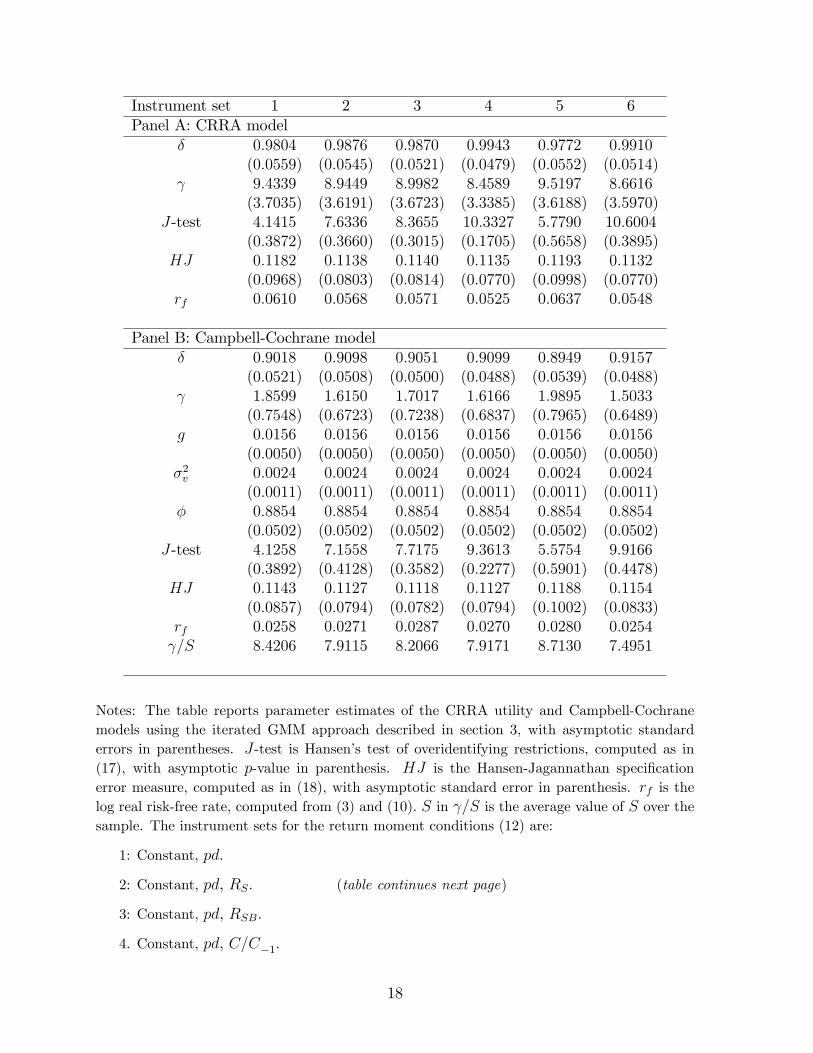
Now we turn to formal estimation of the parameters and statistical tests of the models.Table 3 reports the iterated GMM estimates and associated test statistics for the longannual data set, while Tables 4 and 5 report the results for the shorter quarterly data.We report results using six di¤erent instrument sets for the return moment conditions,see the notes to Table 3. For the annual data, the vector of returns includes real returnson stocks, long-term bonds, and short-term bonds. For the standard CRRA utilitymodel, Panel A in Table 3 shows that the annual subjective discount factor � is preciselyestimated at slightly below unity. The estimated risk-aversion parameter is around8-9 and statistically signi�cant. The J-test does not in any case reject the model atconventional signi�cance levels, and the HJ measure indicates pricing errors of around11%. The annual real risk-free rate, rf , implied by these estimates is around 6%, whichis high but not completely unreasonable.
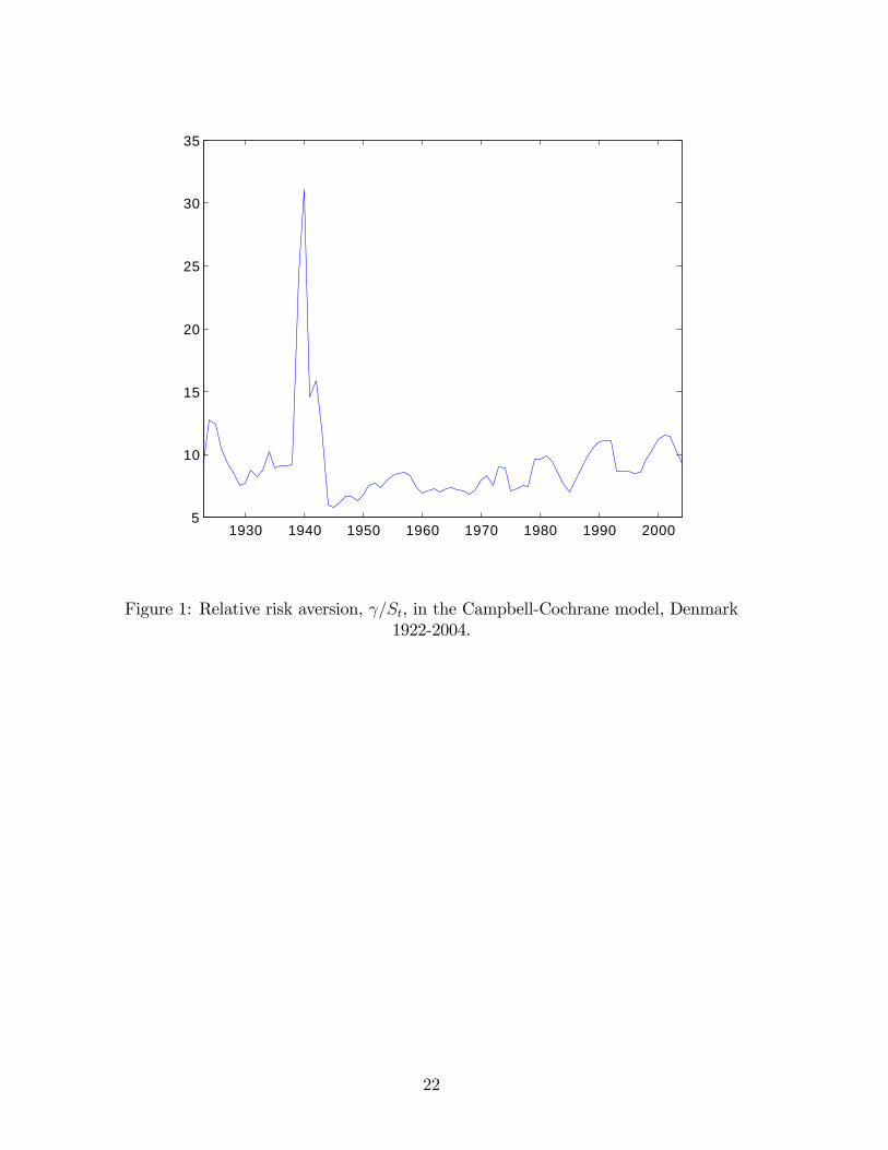
The estimates in Panel B of Table 3 do not indicate that the Campbell-Cochranemodel performs better than the simple CRRA model. The model is not statisticallyrejected and pricing errors and average risk-aversion are of the same magnitude as forthe CRRA model. However, the estimates of � of around 0.90 (implying an annual rateof time-preference of 10%) is somewhat low. On the other hand, the implied risk-freerate of around 2.7% is more reasonable than the 6% implied by the CRRA model. Theestimated average geometric per capita consumption growth rate, g, is 1.56% p.a., witha standard deviation, �v, of around 5% (�2v = 0:0024), and the estimated persistenceparameter of � = 0:88 implies that the price-dividend ratio and, hence, the surplusconsumption ratio are stationary but highly persistent. Figure 1 shows the movementover time in the implied degree of relative risk-aversion, =S, computed from column2 in Table 3, Panel B.5 There is no systematic strong counter-cyclical time-variation inrelative risk-aversion; the most interesting aspect of the �gure is the dramatic increasein risk-aversion associated with the decline in real consumption at the outbreak of WorldWar II. Overall, based on these annual results, it is impossible to discriminate betweenthe CRRA and Campbell-Cochrane models.
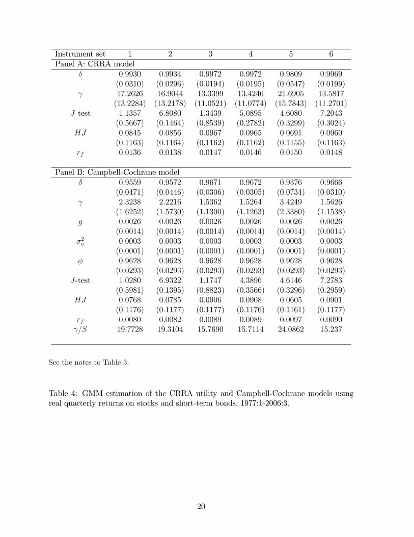
Turning to the quarterly data, Table 4 reports results for stocks and short-term bondsover the period 1977:1-2006:3. As for the annual data, neither the CRRA model nor theCampbell-Cochrane model are statistically rejected by the J-test, and HJ pricing errorsare quite low (below 10%) for both models. The estimated quarterly time discount factor� is reasonable for the CRRA model, but implausibly low for the Campbell-Cochrane
5The time-series movement in =St is essentially similar to the one in Figure 1 if parameter valuesfrom the other columns in Table 3 are used. This also holds for Figures 2 and 3 below.
11

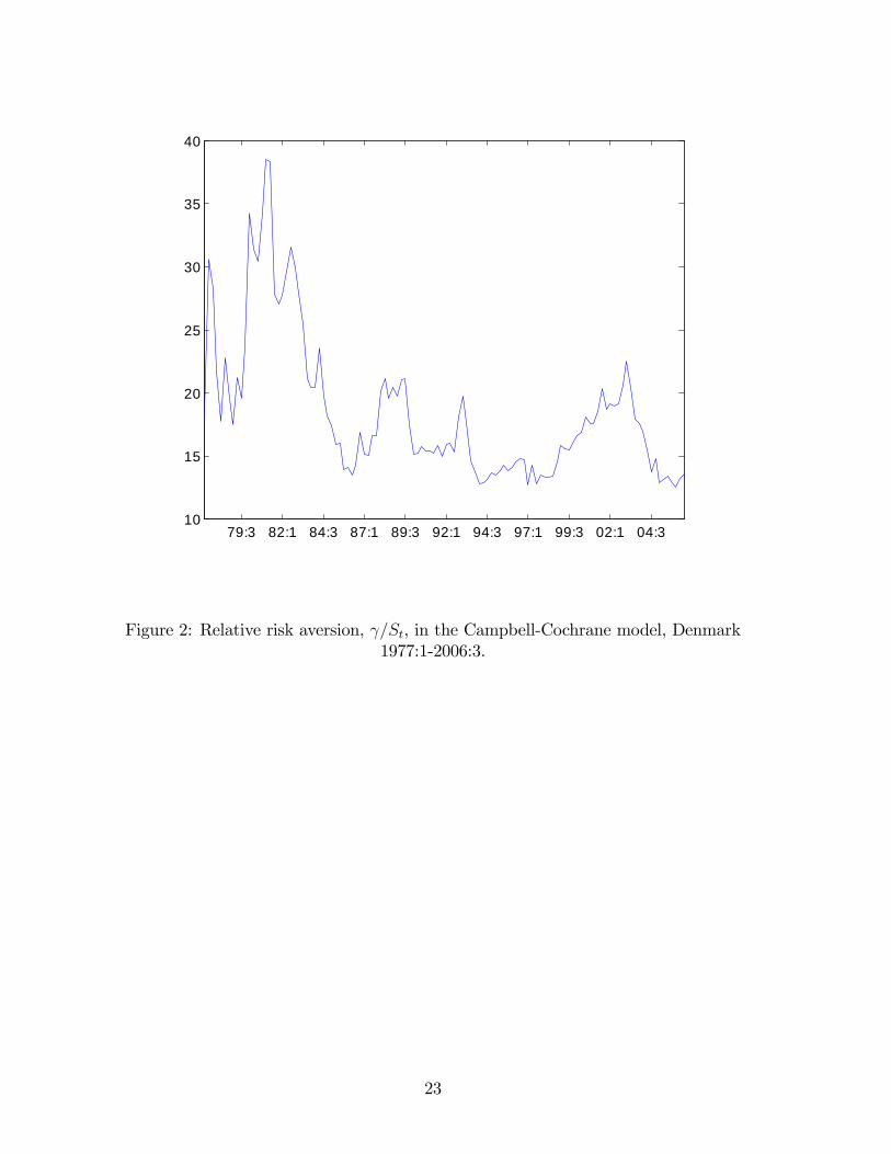
model. The real quarterly risk-free rate is around 1% in both models. In the CRRAmodel, the degree of risk-aversion is very high � ranging from 13 to 22, depending onthe instrument set � but imprecisely estimated. In the Campbell-Cochrane model theestimated values of imply an average degree of risk-aversion from 15 to 24, similar to theestimated values for the CRRA model. However, Figure 2 shows that � in contrast to theannual data � the Campbell-Cochrane model now produces visible counter-cyclical time-variation in the degree of risk-aversion: High risk-aversion during the cyclical downturnsin the late 1970s, beginning of the 1980s, late 1980�s, and start of the new millennium.And low risk-aversion during the booming years of the mid 1980s, mid to late 1990s andthe �nal years of the sample, 2005-2006. (Figure 2 uses the parameter values from column2 in Table 4, Panel B).
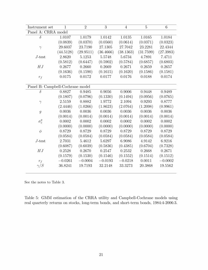
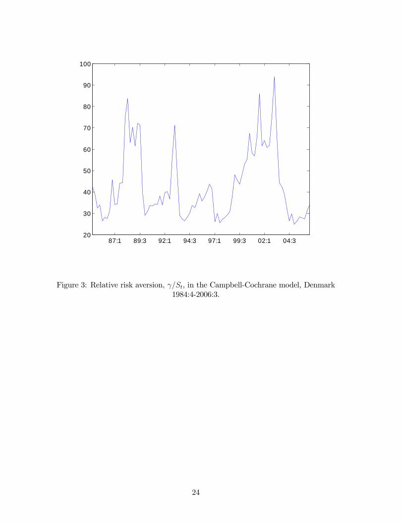
In Table 5 and Figure 3 we include in the return vector long-term bonds in addition tostocks and short-term bonds, and we look at the shorter quarterly sample period, 1984:4-2006:3, since there are no quarterly return data for long-term bonds before 1984:4. Themain di¤erences to the quarterly results in Table 4 and Figure 2 are that now � exceedsone in the CRRAmodel, rf is slightly negative in the Campbell-Cochrane model, andHJpricing errors increase to around 25% for both models even though the J-test still does notreject the models statistically. This is an illustration of the fact emphasized by Hansenand Jagannathan (1997), Cochrane (2005), and others, that a statistical non-rejectionby the J-test does not necessarily imply low pricing errors. Figure 3 resembles Figure2 in showing counter-cyclical time-variation in the degree of risk-aversion, in accordancewith the predictions of the Campbell-Cochrane model.
The main conclusion we draw from the empirical analysis is that for Denmark theCampbell-Cochrane habit formation model does not seem to perform markedly betterthan the standard time-separable power utility model in explaining stock and bond re-turns. For the long annual sample period covering more than 80 years there is ab-solutely no evidence of superior performance of the Campbell-Cochrane model. For theshorter and more recent quarterly data over a 20-30 year period, there is some evidenceof counter-cyclical time-variation in the degree of risk-aversion, in accordance with theCampbell-Cochrane model, but the model does not produce lower pricing errors thanthe time-separable model with constant risk-aversion. Further, the Campbell-Cochranemodel resembles the standard time-separable power utility model in the sense that it hasto rely on very high values of risk-aversion to explain the Danish asset returns.6
5 Concluding remarks
The habit persistence model developed by Campbell and Cochrane (1999) has becomeone of the most prominent consumption based asset pricing models, in particular with
6The risk-aversion estimates reported in this study may be perceived as implausibly high. However,they are not higher than in other studies; see e.g. Campbell (2003) for a comprehensive internationalstudy. In fact, our yearly estimates are much lower than in other studies and do not exceed 10 consideredplausible by Mehra and Prescott (1985).
12

respect to aggregate stock market returns. It explains pro-cyclical stock prices, time-varying and counter-cyclical expected returns, and high and time-varying equity premiaas a result of high but time-varying and counter-cyclical risk-aversion, and it does thiswhile keeping the risk-free rate low and stable.
When the Campbell-Cochrane model is calibrated to actual historical data from theUS, the model is found to match a number of key aspects of the data. However, only a fewattempts have been made to formally estimate and test the model, and almost exclusivelyon US data. These formal estimations and tests generally have led to statistical rejectionof the model. Thus, while there is evidence that the Campbell-Cochrane model hasempirical content on US data, and that it clearly outperforms the standard CRRA utilitymodel, it is also clear that the model does involve signi�cant pricing errors.7
In this paper we have performed a formal econometric estimation and testing ofboth the standard CRRA model and the Campbell-Cochrane model using Danish stockand bond market returns and aggregate consumption. We have used an iterated GMMprocedure that for the Campbell-Cochrane model estimates all parameters in one com-prehensive step while generating � within the iterations � a process for the unobservablesurplus consumption ratio and, hence, the degree of relative risk-aversion.
The results we obtain using this procedure on Danish asset market returns do not ingeneral support the conclusions from the US studies. Although there is some evidence oftime-varying counter-cyclical risk-aversion in recent years, the Campbell-Cochrane modeldoes not produce lower pricing errors or more plausible parameter values than the CRRAmodel. In Engsted et al. (2008) we present further international evidence on the relativeperformance of the two models. There seems to be quite large cross-country di¤erencesin the ability of the Campbell-Cochrane model to explain asset return movements overtime. With no doubt, investigations of consumption-based models with habit persistencewill continue in the future.
7As noted by Campbell and Cochrane (1999) themselves (p.236), the worst performance of the modeloccurs during the end of their sample period, i.e. the �rst half of the 1990s.
13
References
[1] Campbell, J.Y., 2003. Consumption-based asset pricing. In: Constantinides, G.,Harris, M., Stulz, R, Handbook of the economics of �nance. North Holland, Ams-terdam.
[2] Campbell, J.Y., Cochrane, J.H., 1999. By force of habit: A consumption-basedexplanation of aggregate stock market behavior. Journal of Political Economy 107,205-251.
[3] Chen, X., Ludvigson, S.C., 2006. Land of addicts? An empirical investigation ofhabit-based asset pricing models. Working paper, New York University.
[4] Cochrane, J.H., 2005. Asset Pricing (revised edition). Princeton University Press.
[5] Dimson, E., Marsh, P., Staunton, M., 2002. Triumph of the optimists: 101 years ofglobal investment returns. Princeton University Press.
[6] Engsted, T., 2002. Measures of �t for rational expectations models. Journal of Eco-nomic Surveys 16, 301-355.
[7] Engsted, T., Tanggard, C, 1999. The equity premium on Danish stocks (in Danish).Journal of the Danish Economic Association (Nationaløkonomisk Tidsskrift) 137,164-177.
[8] Engsted, T., Hyde, S., Møller, S.V., 2008. Habit formation, surplus consumption,and return predictability: International evidence. Working paper, University ofAarhus.
[9] Ferson, W.E, Harvey, C.R, 1992. Seasonality and consumption asset pricing. Journalof Finance 48, 511-552.
[10] Fillat, J., Garduño, H., 2005. GMM estimation of an asset pricing model with habitpersistence. Working paper. University of Chicago.
[11] Garcia, R., Renault, É., Semenov, A., 2005. A consumption CAPM with a referencelevel. Working paper. CIRANO and Université de Montréal.
[12] Hansen, L.P., 1982. Large sample properties of generalized method of momentsestimators. Econometrica 50, 1029-1054.
[13] Hansen, L.P., Jagannathan, R., 1997. Assessing speci�cation errors in stochasticdiscount factor models. Journal of Finance 52, 557-590.
[14] Hansen, L.P., Heaton, J., Luttmer, E., 1995. Econometric evaluation of asset pricingmodels. Review of Financial Studies 8, 237-274.
[15] Hyde, S., Sherif, M., 2005. Consumption asset pricing models: Evidence from theUK. The Manchester School 73, 343�363.
14

[16] Hyde, S., Cuthbertson, K., Nitzsche, D., 2005. Resuscitating the C-CAPM: Em-pirical evidence from France and Germany. International Journal of Finance andEconomics 10, 337�357.
[17] Li, Y., Zhong, M., 2005. Consumption habit and international stock returns. Journalof Banking and Finance 29, 579-601.
[18] Mehra, R., Prescott, E.C., 1985. The equity premium: A puzzle. Journal of MonetaryEconomics 15, 145-161.
[19] Møller, S.V., 2008. Habit persistence: Explaining cross-sectional variation in returnsand time-varying expected returns. Working paper, Aarhus School of Business, Uni-versity of Aarhus.
[20] Newey, W.K., West, K.D., 1987. A simple, positive semide�nite, heteroskedasticityand autocorrelation consistent covariance matrix. Econometrica 55, 703-708.
[21] Tallarini, T.D., Zhang, H.H., 2005. External habit and the cyclicality of expectedstock returns. Journal of Business 78, 1023-1048.
15
Mean (std.dev) Autocorr. (std.err)Annual, 1922-2004
RS 1:0672 (0:2094) �0:0963 (0:1104)RLB 1:0444 (0:1203) 0:0468 (0:1104)RSB 1:0240 (0:0523) 0:5924 (0:1104)C=C�1 1:0162 (0:0484) 0:1149 (0:1104)pd 3:3211 (0:4631) 0:8836 (0:1104)
Quarterly, 1977:1-2006:3RS 1:0266 (0:0979) 0:2462 (0:0921)RSB 1:0142 (0:0112) 0:7593 (0:0921)C=C�1 1:0031 (0:0165) �0:1449 (0:0921)pd 3:8137 (0:4944) 0:9730 (0:0921)
Quarterly, 1984:4-2006:3RS 1:0286 (0:0941) 0:1806 (0:1072)RLB 1:0193 (0:0319) 0:4086 (0:1072)RSB 1:0122 (0:0109) 0:8542 (0:1072)C=C�1 1:0037 (0:0134) �0:0682 (0:1072)pd 4:0434 (0:2407) 0:8769 (0:1072)
Notes: RS , RLB, and RSB are real gross returns on stocks, long-term bonds, and short-termbonds. C=C�1 is the real per capita gross consumption growth rate. pd is the log price-dividendratio.
Table 1: Summary statistics for asset returns and instruments.
16
Corr(RS, MCRRA) Corr(RS, MCC)Annual, 1922-2004
= 1 �0:1803 = 0:5 �0:1903 = 5 �0:1603 = 1 �0:1649 = 10 �0:1188 = 1:5 �0:1460 = 20 �0:0699 = 2 �0:1309
Quarterly, 1977:1-2006:3 = 1 �0:1332 = 0:5 �0:1118 = 5 �0:1317 = 1 �0:1323 = 10 �0:1290 = 1:5 �0:1368 = 20 �0:1210 = 2 �0:1371
Quarterly, 1984:4-2006:3 = 1 �0:1286 = 0:5 �0:0991 = 5 �0:1195 = 1 �0:0810 = 10 �0:1079 = 1:5 �0:0751 = 20 �0:0845 = 2 �0:0763
Notes: MCRRA and MCC are the stochastic discount factors in the CRRA utility model andCampbell-Cochrane model, respectively.
Table 2: Correlations between stock returns and the stochastic discount factor.
17
Instrument set 1 2 3 4 5 6Panel A: CRRA model
� 0:9804 0:9876 0:9870 0:9943 0:9772 0:9910(0:0559) (0:0545) (0:0521) (0:0479) (0:0552) (0:0514)
9:4339 8:9449 8:9982 8:4589 9:5197 8:6616(3:7035) (3:6191) (3:6723) (3:3385) (3:6188) (3:5970)
J-test 4:1415 7:6336 8:3655 10:3327 5:7790 10:6004(0:3872) (0:3660) (0:3015) (0:1705) (0:5658) (0:3895)
HJ 0:1182 0:1138 0:1140 0:1135 0:1193 0:1132(0:0968) (0:0803) (0:0814) (0:0770) (0:0998) (0:0770)
rf 0:0610 0:0568 0:0571 0:0525 0:0637 0:0548
Panel B: Campbell-Cochrane model� 0:9018 0:9098 0:9051 0:9099 0:8949 0:9157
(0:0521) (0:0508) (0:0500) (0:0488) (0:0539) (0:0488) 1:8599 1:6150 1:7017 1:6166 1:9895 1:5033
(0:7548) (0:6723) (0:7238) (0:6837) (0:7965) (0:6489)g 0:0156 0:0156 0:0156 0:0156 0:0156 0:0156
(0:0050) (0:0050) (0:0050) (0:0050) (0:0050) (0:0050)�2v 0:0024 0:0024 0:0024 0:0024 0:0024 0:0024
(0:0011) (0:0011) (0:0011) (0:0011) (0:0011) (0:0011)� 0:8854 0:8854 0:8854 0:8854 0:8854 0:8854
(0:0502) (0:0502) (0:0502) (0:0502) (0:0502) (0:0502)J-test 4:1258 7:1558 7:7175 9:3613 5:5754 9:9166
(0:3892) (0:4128) (0:3582) (0:2277) (0:5901) (0:4478)HJ 0:1143 0:1127 0:1118 0:1127 0:1188 0:1154
(0:0857) (0:0794) (0:0782) (0:0794) (0:1002) (0:0833)rf 0:0258 0:0271 0:0287 0:0270 0:0280 0:0254 =S 8:4206 7:9115 8:2066 7:9171 8:7130 7:4951
Notes: The table reports parameter estimates of the CRRA utility and Campbell-Cochranemodels using the iterated GMM approach described in section 3, with asymptotic standarderrors in parentheses. J -test is Hansen�s test of overidentifying restrictions, computed as in(17), with asymptotic p-value in parenthesis. HJ is the Hansen-Jagannathan speci�cationerror measure, computed as in (18), with asymptotic standard error in parenthesis. rf is thelog real risk-free rate, computed from (3) and (10). S in =S is the average value of S over thesample. The instrument sets for the return moment conditions (12) are:
1: Constant, pd.
2: Constant, pd, RS . (table continues next page)
3: Constant, pd, RSB.
4. Constant, pd, C=C�1.
18

5. Constant, pd, and its lag.
6. Constant, pd, RS , RSB.
Table 3: GMM estimation of the CRRA utility and Campbell-Cochrane models usingreal annual returns on stocks, long-term bonds, and short-term bonds, 1922-2004.
19
Instrument set 1 2 3 4 5 6Panel A: CRRA model
� 0:9930 0:9934 0:9972 0:9972 0:9809 0:9969(0:0310) (0:0296) (0:0194) (0:0195) (0:0547) (0:0199)
17:2626 16:9044 13:3399 13:4246 21:6905 13:5817(13:2284) (13:2178) (11:0521) (11:0774) (15:7843) (11:2701)
J-test 1:1357 6:8080 1:3439 5:0895 4:6080 7:2043(0:5667) (0:1464) (0:8539) (0:2782) (0:3299) (0:3024)
HJ 0:0845 0:0856 0:0967 0:0965 0:0691 0:0960(0:1163) (0:1164) (0:1162) (0:1162) (0:1155) (0:1163)
rf 0:0136 0:0138 0:0147 0:0146 0:0150 0:0148
Panel B: Campbell-Cochrane model� 0:9559 0:9572 0:9671 0:9672 0:9376 0:9666
(0:0471) (0:0446) (0:0306) (0:0305) (0:0734) (0:0310) 2:3238 2:2216 1:5362 1:5264 3:4249 1:5626
(1:6252) (1:5730) (1:1300) (1:1263) (2:3380) (1:1538)g 0:0026 0:0026 0:0026 0:0026 0:0026 0:0026
(0:0014) (0:0014) (0:0014) (0:0014) (0:0014) (0:0014)�2v 0:0003 0:0003 0:0003 0:0003 0:0003 0:0003
(0:0001) (0:0001) (0:0001) (0:0001) (0:0001) (0:0001)� 0:9628 0:9628 0:9628 0:9628 0:9628 0:9628
(0:0293) (0:0293) (0:0293) (0:0293) (0:0293) (0:0293)J-test 1:0280 6:9322 1:1747 4:3896 4:6146 7:2783
(0:5981) (0:1395) (0:8823) (0:3566) (0:3296) (0:2959)HJ 0:0768 0:0785 0:0906 0:0908 0:0605 0:0901
(0:1176) (0:1177) (0:1177) (0:1176) (0:1161) (0:1177)rf 0:0080 0:0082 0:0089 0:0089 0:0097 0:0090 =S 19:7728 19:3104 15:7690 15:7114 24:0862 15:237
See the notes to Table 3.
Table 4: GMM estimation of the CRRA utility and Campbell-Cochrane models usingreal quarterly returns on stocks and short-term bonds, 1977:1-2006:3.
20
Instrument set 1 2 3 4 5 6Panel A: CRRA model
� 1:0107 1:0179 1:0142 1:0135 1:0165 1:0184(0:0839) (0:0370) (0:0560) (0:0614) (0:0371) (0:0323)
29:6037 23:7190 27:1305 27:7042 23:2281 22:4344(44:5128) (29:9511) (36:4666) (38:1363) (31:7599) (27:3983)
J-test 2:8620 5:1253 5:5748 5:6734 4:7891 7:4711(0:5812) (0:6447) (0:5902) (0:5784) (0:6857) (0:6803)
HJ 0:2677 0:2660 0:2669 0:2671 0:2659 0:2657(0:1636) (0:1590) (0:1615) (0:1620) (0:1586) (0:1581)
rf 0:0175 0:0172 0:0177 0:0176 0:0188 0:0174
Panel B: Campbell-Cochrane model� 0:8827 0:9485 0:9056 0:9006 0:9448 0:9489
(0:1807) (0:0796) (0:1330) (0:1494) (0:0956) (0:0765) 2:5159 0:8882 1:9772 2:1094 0:9293 0:8777
(2:4446) (1:0266) (1:8623) (2:0764) (1:2098) (0:9961)g 0:0036 0:0036 0:0036 0:0036 0:0036 0:0036
(0:0014) (0:0014) (0:0014) (0:0014) (0:0014) (0:0014)�2v 0:0002 0:0002 0:0002 0:0002 0:0002 0:0002
(0:0000) (0:0000) (0:0000) (0:0000) (0:0000) (0:0000)� 0:8729 0:8729 0:8729 0:8729 0:8729 0:8729
(0:0584) (0:0584) (0:0584) (0:0584) (0:0584) (0:0584)J-test 2:7031 5:4612 5:6297 6:9086 4:9142 6:9216
(0:6087) (0:6039) (0:5836) (0:4385) (0:6704) (0:7328)HJ 0:2528 0:2670 0:2547 0:2532 0:2668 0:2671
(0:1579) (0:1530) (0:1546) (0:1552) (0:1514) (0:1512)rf �0:0261 �0:0004 �0:0193 �0:0218 0:0011 �0:0002 =S 36:8241 19:7193 32:2148 33:3273 20:3868 19:5562
See the notes to Table 3.
Table 5: GMM estimation of the CRRA utility and Campbell-Cochrane models usingreal quarterly returns on stocks, long-term bonds, and short-term bonds, 1984:4-2006:3.
21
1930 1940 1950 1960 1970 1980 1990 20005
10
15
20
25
30
35
Figure 1: Relative risk aversion, =St, in the Campbell-Cochrane model, Denmark1922-2004.
22
79:3 82:1 84:3 87:1 89:3 92:1 94:3 97:1 99:3 02:1 04:310
15
20
25
30
35
40
Figure 2: Relative risk aversion, =St, in the Campbell-Cochrane model, Denmark1977:1-2006:3.
23
87:1 89:3 92:1 94:3 97:1 99:3 02:1 04:320
30
40
50
60
70
80
90
100
Figure 3: Relative risk aversion, =St, in the Campbell-Cochrane model, Denmark1984:4-2006:3.
24

Chapter 2
Habit persistence: Explaining cross-sectional variation in returns andtime-varying expected returns
Habit persistence: Explaining cross-sectionalvariation in returns and time-varying expected
returns�
Stig Vinther Møllery
Invited for third resubmission to the Journal of Empirical Finance.
Abstract
This paper uses an iterated GMM approach to estimate and test the consump-tion based habit persistence model of Campbell and Cochrane (1999) on the USstock market. The empirical evidence shows that the model is able to explain thesize premium, but fails to explain the value premium. Further, the state variableof the model � the surplus consumption ratio � explains counter-cyclical time-varying expected returns on stocks. The model also produces plausible low realrisk-free rates despite high relative risk aversion.
Keywords: Campbell-Cochrane model, 25 Fama-French portfolios, GMM, returnpredictability by surplus consumption ratio.JEL codes: C32, G12.
�I am grateful to Geert Bekaert (the Editor), John Cochrane, Tom Engsted, Domenico De Giovanni,Stuart Hyde, Jesper Rangvid, Carsten Tanggaard, and two anonymous referees for their insightful com-ments. I would also like to thank participants at the 20th Australasian Finance and Banking Conferencein Sydney, the Nordic Finance Network Research Workshop in Helsinki, and the CREATES symposium"New hope for the C-CAPM?".
yDepartment of Business Studies, Aarhus School of Business, University of Aarhus, Fuglesangs Allé4, DK-8210 Aarhus V., Denmark and Center for Research in Econometric Analysis of Time Series (CRE-ATES) funded by the Danish National Research Foundation. E-mail: [email protected]. Tel.: +4589486188.
1

1 Introduction
Within the consumption based asset pricing framework, the habit persistence model ofCampbell and Cochrane (1999) model has become one of the leading models in explainingasset pricing behavior. The Campbell-Cochrane model explains a number of stylizedfacts on the US stock market, including pro-cyclical stock prices, time-varying counter-cyclical expected returns, and it has the ability to explain the equity premium puzzlewithout facing a risk-free rate puzzle. Campbell and Cochrane and most subsequentapplications of their model rely on calibration and simulation exercises and do not engagein formal econometric estimation and testing of the model. They calibrate the structuralparameters of the model to match historical means of the risk-free rate and the Sharperatio, and then simulate a chosen set of moments which are informally compared to thosebased on the actual historical data.
Instead of calibrating and simulating the Campbell-Cochrane model, this paper usesan iterated GMM approach to estimate and test the model on the US stock marketover the period 1947-2005. The model is estimated in a cross-sectional setting using the25 Fama and French value and size portfolios, which has not been tried previously, cf.Cochrane (2007). Following the suggestion of Lewellen et al. (2008), the portfolio set isexpanded beyond the value and size dimensions by including 10 industry portfolios. Theestimation of the model reveals that it has di¢ culties in explaining the value premium,but provides a great �t of the size premium. The inability of the model to explain thevalue premium is consistent with recent work by Lettau and Wachter (2007) and Santosand Veronesi (2008). They argue that due to the negative correlation between changesin consumption and the price of risk, the Campbell-Cochrane model is likely to generatea growth premium instead of a value premium.
Besides cross-sectional variation in stock returns, the paper examines whether themodel captures time-variation in expected stock returns. The Campbell-Cochrane modelhas the intuitively appealing implication that expected stock returns vary counter-cyclicallyover the business cycle. As a result, investors require a higher expected stock return inrecession times when consumption is close to habit. The empirical evidence shows thatthe surplus consumption ratio is signi�cantly negatively related to future excess stock re-turns, implying that low surplus consumption � when consumption gets close to habit inrecession times � predicts high future excess stock returns. These �ndings are consistentwith Li (2001, 2005) who uses Campbell and Cochrane�s calibrated parameter values toexamine the predictive power of the surplus consumption ratio.
Following the suggested extension in Wachter (2006), the paper allows for a time-varying real risk-free rate in order to generate cyclical variation in interest rates and anontrivial term structure. Despite high relative risk aversion, the Campbell-Cochranemodel implies plausible low values for the real risk-free rate, i.e. the model explains theequity premium puzzle without facing a risk-free rate puzzle. However, the estimatedstructural parameters of the model imply counterfactual implications for the slope of theyield curve.
2
Only a few papers engage in formal econometric estimation of the Campbell-Cochranemodel. Fillat and Garduño (2005), Garcia et al. (2005), and Tallarini and Zhang (2005)estimate the model on US data.1 However, they all consider the baseline version of themodel with a constant real risk-free rate and only use a small cross section of equities.This paper di¤ers by allowing for time-variation in the real risk-free rate and by testingwhether the model accounts for the cross-sectional variation in returns on value, size andindustry portfolios, as well as variation of expected returns over time.2
The paper relates to Bekaert et al. (2005), Buraschi and Jiltsov (2007), and Wachter(2006) who explore extensions of the Campbell-Cochrane model to explain the full termstructure of interest rates. Moreover, Verdelhan (2008) extends the Campbell-Cochranemodel to explain the foreign exchange risk premium. Bekaert et al. (2007) considertime-varying counter-cyclical risk aversion as well as economic uncertainty as sources ofrisk and �nd that both are important in explaining many asset pricing phenomena.3
The paper also relates to the growing body of literature documenting time-varying ex-pected stock returns. Financial variables such as the price-dividend ratio, the term spreadon bonds, and the relative interest rate have been documented as forecasters of stock re-turns, cf. Campbell and Shiller (1988), Fama and French (1989), Campbell (1991), andHodrick (1992). Fama and French (1989) link the �nancial forecasting variables to thebusiness cycle and suggest that investors require a higher expected return at a businesscycle trough than they do at a business cycle peak. As an extension to these �nancialforecasting variables, Lettau and Ludvigson (2001) introduce the consumption-wealthratio, which is a macroeconomic variable that forecasts stock returns. Similarly, the sur-plus consumption ratio in the Campbell-Cochrane model is a macroeconomic variablethat provides a direct linkage between the business cycle and expected stock returns.
The paper is organized as follows. Section 2 introduces the Campbell-Cochrane model,Section 3 describes the empirical methodology, Section 4 describes the data, Section 5reports the empirical results, and Section 6 concludes.
2 The Campbell-Cochrane model
The utility function of the representative investor is:
Et
1Xj=0
�j(Ct+j �Xt+j)
1� � 11� : (1)
Ct is real consumption, Xt is the external habit level, � is the impatience parameter,and is the utility curvature parameter. Campbell and Cochrane capture the relation
1Engsted and Møller (2008) estimate the model outside the US and �nd that it does not performbetter than the simple CRRA model in explaining Danish asset returns.
2Chen and Ludvigson (2008) also estimate a habit-based model on the 25 Fama and French portfolios,but they treat the functional form of the habit as unknown.
3Bansal and Yaron (2004) develop a long-run risk model and stress the importance of economicuncertainty.
3

between consumption and habit through the surplus consumption ratio:
St �Ct �Xt
Ct; (2)
and specify the logarithm of the surplus consumption ratio st = log (St) as a stationary�rst-order autoregressive process:
st+1 = (1� �) �s+ �st + � (st) vt+1, (3)
where 0 < � < 1 is the habit persistence parameter, �s is the steady state level of st, and� (st) is the sensitivity function that determines how innovations in consumption growthvt+1 in�uence st+1. The consumption growth process is given by:
4ct+1 = g + vt+1; vt+1 � niid�0; �2c
�, (4)
where ct = log (Ct), and g is the mean consumption growth rate. The sensitivity function�(st) is speci�ed as follows:
� (st) =
8><>:1�S
p1� 2 (st � �s)� 1; st � smax
0 st � smax
9>=>; , (5)
where
S = �c
r
1� ��B= ; smax = s+1
2(1� S2); s = log(S):
Specifying � (st) in this way implies that the real risk-free rate is a linear function of st.From the Euler equation,
1 = Et [Ri;t+1Mt+1] , (6)
where Ri;t+1 is the real gross return on any asset i, and Mt+1 is the stochastic discountfactor:
Mt+1 = �
�St+1St
Ct+1Ct
�� = �e� fg+(��1)(st�s)+[1+�(st)]vt+1g; (7)
the log real risk-free rate is:
rf;t+1 = log
�1
Et [Mt+1]
�(8)
= � log (�) + g � (1� �)�B2
�B (st � s) : (9)
B governs the cyclicality of the real risk-free rate and the slope of the yield curve. B > 0implies a counter-cyclical real risk-free rate and an upward-sloping yield curve. B < 0implies a pro-cyclical real risk-free rate and a downward-sloping yield curve. B = 0corresponds to the baseline version of the Campbell-Cochrane model with a constantreal risk-free rate.
4
From the Euler equation (6), the expected excess stock return can be stated as:
Et�rei;t+1
�+1
2�2i;t = [1 + � (st)]�ic;t, (10)
where 12�2i;t is a Jensen�s inequality term. (10) shows that the expected excess stock
return is given by the state-dependent price of risk, [1 + � (st)], times the amount ofrisk, �ic;t (the conditional covariance between the return on asset i and the consumptiongrowth). Li (2001) �nds that �ic;t is close to being constant through time. This lackof time-variation in the amount of risk suggests that time-varying expected excess stockreturns are generated entirely by time-variation in the price of risk. Since � (st) is de-creasing in st, it follows that expected excess stock returns vary counter-cyclically withst. Thus, investors require a higher expected excess stock return in recession times whenconsumption is close to habit.
3 Empirical methodology
The Campbell-Cochrane model is estimated using Hansen�s (1982) GMM based on thefollowing moment conditions:
0N�1 = E�Rt+1�e
� fg+(��1)(st�s)+[1+�(st)]vt+1g � 1�; (11)
02�1 = E��ret+1 � �� �st�1
�(1 st�1)
0� ; (12)
0 = E
�rf;t+1 + log (�)� g +
(1� �)�B2
+B (st � s)�; (13)
0 = E
24(y2;t � rf;t+1) + 12
24 �0:5( (1� �)�B)+( (1� �) +B(�� 2))(st � �s)+0:5�2c [B� (st)� � � (st)]
2
3535 ; (14)
0 = E [4ct+1 � g] ; (15)
0 = E�(4ct+1 � g)2 � �2c
�: (16)
The moment conditions are chosen in order to examine whether the Campbell-Cochranemodel simultaneously explains the cross-sectional variation in returns on stocks, time-varying expected returns on stocks, and the mean values of the real risk-free rate andthe real yield spread.
First, using the Euler equation (6) and the stochastic discount factor in (7), I formthe moment conditions in (11), where Rt+1 contains real gross returns on a vector of Nassets. The purpose is to examine whether the model is able to explain the cross-sectionalvariation in mean stock returns on portfolios sorted on size, book-to-market and industry.The returns are not scaled with instruments since this would result in an unmanageablelarge number of moment conditions relative to the number of sample observations.
5
Second, in order to examine whether the model captures time-variation in expectedstock returns, I form the moment conditions in (12). By approximating equation (10),I examine the linear relationship between the surplus consumption ratio and the futureexcess stock return.4 Li (2005) also examines the linear predictive power of the surplusconsumption ratio, but uses the calibrated parameter values of Campbell and Cochrane(1999) to generate the surplus consumption ratio. Since the surplus consumption ratio isestimated using Campbell�s (2003) beginning of period consumption timing convention,it is lagged twice in (12).
Third, I examine whether the model is able to explain the mean values of the realrisk-free rate and the real yield spread. In this way GMM estimates the model parametersbased on both stock and bond market data. Using the speci�cation of the real risk-freerate in (8), I obtain the moment condition in (13), and using the analytical solution ofthe 2-year yield spread shown in the appendix, I obtain the moment condition in (14). Irestrict the attention to the 2-year yield spread because it is not possible to �nd analyticalsolutions for a higher maturity than 2 years.
Finally, given the random walk model of consumption in (4), I estimate the meanof the consumption growth rate and its volatility based on moment conditions (15) and(16) :
The estimation of the Campbell-Cochrane model is complicated by the fact that thesurplus consumption ratio is not observable in the same way as returns and consumptionare directly observable. To observe the st process, I use s0 = s as starting value of st att = 0. Then I choose initial values of the model parameters from which the st process canbe constructed using (3). By iterating over the model parameters, the GMM proceduresimultaneously generates the st process and estimates the model parameters.
De�ning gT (�) as the sample moment conditions based on T observations, the para-meter vector � = (� � B g �c � �)0 is estimated by minimizing the quadraticform:
gT (�)0WgT (�) , (17)
where W is a positive de�nite weighting matrix. The identity matrix, I, is used to giveequal weight to all moment conditions.
Since the chosen weighting matrix is not the e¢ cient Hansen (1982) matrix but theidentity matrix, the formula for the covariance matrix of the parameter vector is (cf.Cochrane (2005), chpt. 11):
V ar(b�) = 1
T(d0Id)�1d0ISId(d0Id)�1; (18)
where d0 = @gT (�)=@�, and the spectral density matrix S =P1
j=�1E[ gT (�)gT�j(�)0]
is computed with the usual Newey and West (1987) estimator with a lag truncation.Similarly, the J-test of overidentifying restrictions is computed based on the general
4The GMM moment conditions in (12) correspond to the normal OLS equations used in the returnpredictability literature.
6
formula (cf. Cochrane (2005) chpt. 11):
JT = TgT (b�)0 �(I � d(d0Id)�1d0I)S(I � Id(d0Id)�1d0)��1 gT (b�): (19)
JT has an asymptotic �2 distribution with degrees of freedom equal to the number ofoveridentifying restrictions. (19) involves the covariance matrix V ar(gT (b�)) = 1
T(I �
d(d0Id)�1d0I)S(I � Id(d0Id)�1d0), which is singular, so it is inverted using the Moore-Penrose pseudo-inversion.
As a measure of the cross-sectional �t, the root mean squared error across the Nassets is used:
RMSE =
s1
N
NPi=1
��Ri � E [Ri]
�2; (20)
where �Ri is the average return on asset i, and E [Ri] is the model predicted average returnon asset i.
As a measure of the predictive power of the surplus consumption ratio, the R2-statisticis used:
R2 =V ar (�st�1)
V ar�ret+1
� : (21)
4 Data
The Campbell-Cochrane model is estimated on annual post-war data for the period1947 to 2005. Consumption is measured as expenditures on non-durables and servicesobtained from the National Income and Product Accounts (NIPA) table 2.3.5. Followingthe beginning of period timing convention of Campbell (2003), consumption during yeart is assumed to take place at the beginning of year t. Nominal consumption is convertedto real units using the consumption de�ator from NIPA table 2.3.4. Real per capitaconsumption is obtained using the population numbers in NIPA table 2.1.
The log excess stock return is calculated as the log real return on the value weightedCRSP index including NYSE, AMEX, and NASDAQ �rms minus the log real risk-freerate. The log real risk-free rate (de�ned as the log real 1-year yield) and the log real 2-year yield are based on the McCulloch-Kwon dataset available at J. Huston McCulloch�swebsite and the Fama-Bliss dataset available at the CRSP. The McCulloch-Kwon datasetcontains yield data from 1947 to 1990, and this dataset is extended up to 2005 using theFama-Bliss dataset.
The model is estimated on the 25 Fama and French portfolios sorted on book-to-market and size. Following the suggestion of Lewellen et al. (2008), the portfolio set isexpanded beyond the value and size dimensions by including 10 industry portfolios. Tocheck the robustness, the model is estimated on other portfolios as well. Due to potentialsmall sample problems, the model is estimated on a small cross section of the 6 Fama andFrench portfolios underlying the Fama and French (1993) factors SMB and HML together
7
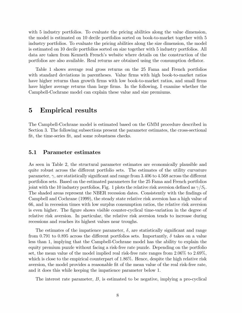
with 5 industry portfolios. To evaluate the pricing abilities along the value dimension,the model is estimated on 10 decile portfolios sorted on book-to-market together with 5industry portfolios. To evaluate the pricing abilities along the size dimension, the modelis estimated on 10 decile portfolios sorted on size together with 5 industry portfolios. Alldata are taken from Kenneth French�s website where details on the construction of theportfolios are also available. Real returns are obtained using the consumption de�ator.
Table 1 shows average real gross returns on the 25 Fama and French portfolioswith standard deviations in parentheses. Value �rms with high book-to-market ratioshave higher returns than growth �rms with low book-to-market ratios, and small �rmshave higher average returns than large �rms. In the following, I examine whether theCampbell-Cochrane model can explain these value and size premiums.
5 Empirical results
The Campbell-Cochrane model is estimated based on the GMM procedure described inSection 3. The following subsections present the parameter estimates, the cross-sectional�t, the time-series �t, and some robustness checks.
5.1 Parameter estimates
As seen in Table 2, the structural parameter estimates are economically plausible andquite robust across the di¤erent portfolio sets. The estimates of the utility curvatureparameter, , are statistically signi�cant and range from 3:406 to 4:568 across the di¤erentportfolios sets. Based on the estimated parameters for the 25 Fama and French portfoliosjoint with the 10 industry portfolios, Fig. 1 plots the relative risk aversion de�ned as =St.The shaded areas represent the NBER recession dates. Consistently with the �ndings ofCampbell and Cochrane (1999), the steady state relative risk aversion has a high value of66, and in recession times with low surplus consumption ratios, the relative risk aversionis even higher. The �gure shows visible counter-cyclical time-variation in the degree ofrelative risk aversion. In particular, the relative risk aversion tends to increase duringrecessions and reaches its highest values near troughs.
The estimates of the impatience parameter, �, are statistically signi�cant and rangefrom 0:791 to 0:895 across the di¤erent portfolios sets. Importantly, � takes on a valueless than 1, implying that the Campbell-Cochrane model has the ability to explain theequity premium puzzle without facing a risk-free rate puzzle. Depending on the portfolioset, the mean value of the model implied real risk-free rate ranges from 2:06% to 2:69%,which is close to the empirical counterpart of 1:86%. Hence, despite the high relative riskaversion, the model provides a reasonable �t of the mean value of the real risk-free rate,and it does this while keeping the impatience parameter below 1.
The interest rate parameter, B, is estimated to be negative, implying a pro-cyclical
8
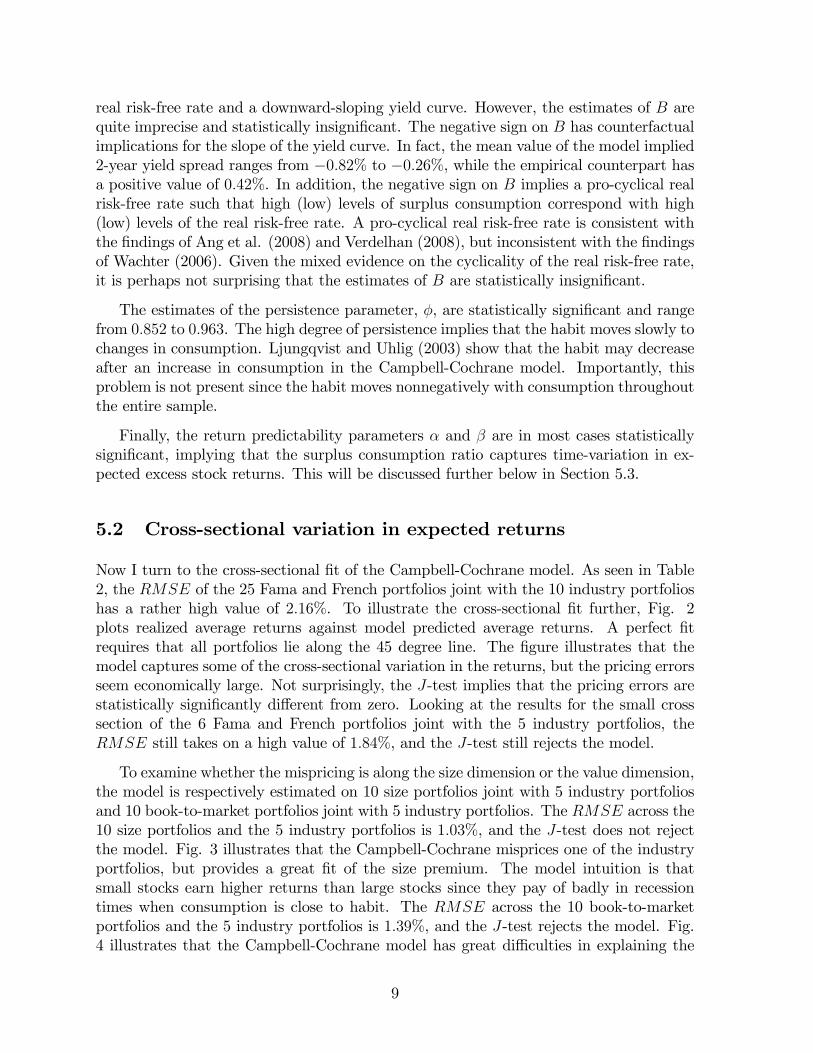
real risk-free rate and a downward-sloping yield curve. However, the estimates of B arequite imprecise and statistically insigni�cant. The negative sign on B has counterfactualimplications for the slope of the yield curve. In fact, the mean value of the model implied2-year yield spread ranges from �0:82% to �0:26%, while the empirical counterpart hasa positive value of 0:42%. In addition, the negative sign on B implies a pro-cyclical realrisk-free rate such that high (low) levels of surplus consumption correspond with high(low) levels of the real risk-free rate. A pro-cyclical real risk-free rate is consistent withthe �ndings of Ang et al. (2008) and Verdelhan (2008), but inconsistent with the �ndingsof Wachter (2006). Given the mixed evidence on the cyclicality of the real risk-free rate,it is perhaps not surprising that the estimates of B are statistically insigni�cant.
The estimates of the persistence parameter, �, are statistically signi�cant and rangefrom 0:852 to 0:963. The high degree of persistence implies that the habit moves slowly tochanges in consumption. Ljungqvist and Uhlig (2003) show that the habit may decreaseafter an increase in consumption in the Campbell-Cochrane model. Importantly, thisproblem is not present since the habit moves nonnegatively with consumption throughoutthe entire sample.
Finally, the return predictability parameters � and � are in most cases statisticallysigni�cant, implying that the surplus consumption ratio captures time-variation in ex-pected excess stock returns. This will be discussed further below in Section 5.3.
5.2 Cross-sectional variation in expected returns
Now I turn to the cross-sectional �t of the Campbell-Cochrane model. As seen in Table2, the RMSE of the 25 Fama and French portfolios joint with the 10 industry portfolioshas a rather high value of 2:16%. To illustrate the cross-sectional �t further, Fig. 2plots realized average returns against model predicted average returns. A perfect �trequires that all portfolios lie along the 45 degree line. The �gure illustrates that themodel captures some of the cross-sectional variation in the returns, but the pricing errorsseem economically large. Not surprisingly, the J-test implies that the pricing errors arestatistically signi�cantly di¤erent from zero. Looking at the results for the small crosssection of the 6 Fama and French portfolios joint with the 5 industry portfolios, theRMSE still takes on a high value of 1:84%, and the J-test still rejects the model.
To examine whether the mispricing is along the size dimension or the value dimension,the model is respectively estimated on 10 size portfolios joint with 5 industry portfoliosand 10 book-to-market portfolios joint with 5 industry portfolios. The RMSE across the10 size portfolios and the 5 industry portfolios is 1:03%, and the J-test does not rejectthe model. Fig. 3 illustrates that the Campbell-Cochrane misprices one of the industryportfolios, but provides a great �t of the size premium. The model intuition is thatsmall stocks earn higher returns than large stocks since they pay of badly in recessiontimes when consumption is close to habit. The RMSE across the 10 book-to-marketportfolios and the 5 industry portfolios is 1:39%, and the J-test rejects the model. Fig.4 illustrates that the Campbell-Cochrane model has great di¢ culties in explaining the
9
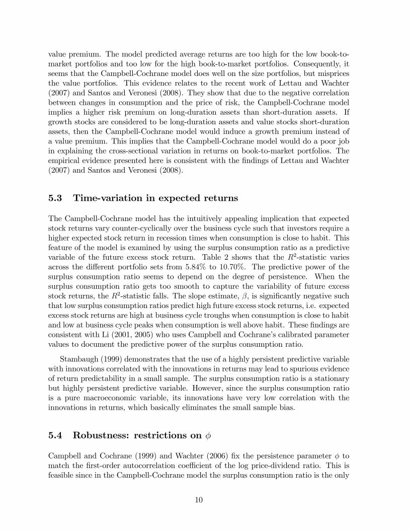
value premium. The model predicted average returns are too high for the low book-to-market portfolios and too low for the high book-to-market portfolios. Consequently, itseems that the Campbell-Cochrane model does well on the size portfolios, but mispricesthe value portfolios. This evidence relates to the recent work of Lettau and Wachter(2007) and Santos and Veronesi (2008). They show that due to the negative correlationbetween changes in consumption and the price of risk, the Campbell-Cochrane modelimplies a higher risk premium on long-duration assets than short-duration assets. Ifgrowth stocks are considered to be long-duration assets and value stocks short-durationassets, then the Campbell-Cochrane model would induce a growth premium instead ofa value premium. This implies that the Campbell-Cochrane model would do a poor jobin explaining the cross-sectional variation in returns on book-to-market portfolios. Theempirical evidence presented here is consistent with the �ndings of Lettau and Wachter(2007) and Santos and Veronesi (2008).
5.3 Time-variation in expected returns
The Campbell-Cochrane model has the intuitively appealing implication that expectedstock returns vary counter-cyclically over the business cycle such that investors require ahigher expected stock return in recession times when consumption is close to habit. Thisfeature of the model is examined by using the surplus consumption ratio as a predictivevariable of the future excess stock return. Table 2 shows that the R2-statistic variesacross the di¤erent portfolio sets from 5:84% to 10:70%. The predictive power of thesurplus consumption ratio seems to depend on the degree of persistence. When thesurplus consumption ratio gets too smooth to capture the variability of future excessstock returns, the R2-statistic falls. The slope estimate, �, is signi�cantly negative suchthat low surplus consumption ratios predict high future excess stock returns, i.e. expectedexcess stock returns are high at business cycle troughs when consumption is close to habitand low at business cycle peaks when consumption is well above habit. These �ndings areconsistent with Li (2001, 2005) who uses Campbell and Cochrane�s calibrated parametervalues to document the predictive power of the surplus consumption ratio.
Stambaugh (1999) demonstrates that the use of a highly persistent predictive variablewith innovations correlated with the innovations in returns may lead to spurious evidenceof return predictability in a small sample. The surplus consumption ratio is a stationarybut highly persistent predictive variable. However, since the surplus consumption ratiois a pure macroeconomic variable, its innovations have very low correlation with theinnovations in returns, which basically eliminates the small sample bias.
5.4 Robustness: restrictions on �
Campbell and Cochrane (1999) and Wachter (2006) �x the persistence parameter � tomatch the �rst-order autocorrelation coe¢ cient of the log price-dividend ratio. This isfeasible since in the Campbell-Cochrane model the surplus consumption ratio is the only
10

state variable, whereby the log price-dividend ratio inherits its dynamic properties fromthe log surplus consumption ratio. It is not possible to �nd an analytical solution of theprice-dividend ratio in the Campbell-Cochrane model. Instead, Campbell and Cochrane(1999) and Wachter (2006) solve the price-dividend ratio numerically based on a gridsearch. Fig. 5 shows the solution of the price-dividend ratio based on the estimatedparameter values from column 2 in Table 2.5 Similarly to the �ndings of Campbell andCochrane (1999) and Wachter (2006), the �gure illustrates that price-dividend ratio is anearly linear function of the surplus consumption ratio.
The strict version of the Campbell-Cochrane model predicts a perfect relationshipbetween the surplus consumption ratio and the price-dividend ratio. In real data, how-ever, the two series do not move one for one, but they are closely related. Fig. 6 showsthat the two series move together quite closely, but to some extent become disconnectedin the �rst part of the 1990s. Campbell and Cochrane (1999) themselves also �nd thatduring the �rst part of the 1990s � the end of their sample period � the calibratedprice-dividend ratio moves in the opposite direction of the actual price-dividend ratio.
Following Campbell and Cochrane (1999) and Wachter (2006), I now �x the persis-tence parameter � to match the �rst-order autocorrelation coe¢ cient of the log price-dividend ratio and reestimate the model. The persistence parameter � is set equal to0.956. The results of this robustness check are shown in Table 3. The table shows thatthe restriction on � does not in�uence the parameter estimates much. The table alsoshows that the restriction on � has very little impact on the cross-sectional �t of themodel. The RMSE is basically unchanged across the di¤erent portfolio sets. The onlychange in the results is that the predictive power of the surplus consumption ratio forfuture excess stock returns is slightly lower.
6 Conclusions
Campbell and Cochrane (1999) show by calibration and simulation that their modelexplains a number of stylized facts on the US stock market. Instead of calibrating andsimulating the model, this paper uses an iterated GMM approach to estimate and testthe model. The GMM estimation of the model shows that it is able to explain the sizepremium, but has great di¢ culties in explaining the value premium. This is consistentwith Lettau and Wachter (2007) and Santos and Veronesi (2008) who show that theCampbell-Cochrane model implies a growth premium due to the negative correlationbetween changes in consumption and the price of risk. While the model has di¢ culties inexplaining cross-sectional variation in expected stock returns, the model has the abilityto explain time-variation in expected stock returns. The model implies that relativerisk aversion and expected stock returns are time-varying and counter-cyclical. When
5I use a �xed-point solution method (written in MatLab) similar to the one used by Campbell andCochrane (1999). I use a �ne grid with 100 linearly spaced points between 0 and Smax, and I also includeSmax in the grid. Wachter (2005) shows that the solution of the price-dividend function converges as thegrid becomes increasingly �ne.
11

consumption is close to habit in recession times, the relative risk aversion is high andinvestors require a higher expected risk premium to invest in stocks. Thus, the modelprovides a direct linkage between time-varying expected stock returns and the businesscycle.
12

7 Appendix
The Euler equation for bonds is:
Pn;t = Et [Pn�1;t+1Mt+1] ;
where Pn;t is the time t real price of a bond with maturity n, and the log real yield isgiven by yn;t = � 1
nlogPn;t. It is possible to �nd closed form solutions for n = 1 and
n = 2, but not for higher values of n. For n = 1 the real price is:
P1;t = Et [P0;t+1Mt+1]
= Et [Mt+1]
= e�rf;t+1 :
where rf;t+1 is known at time t. For n = 2 the real price is:
P2;t = Et [P1;t+1Mt+1]
= Et�e��r+B(st+1��s)�e� fg+(��1)(st�s)+[1+�(st)]vt+1g
�= �e��re� ge( (1��)+B�)(st��s)e0:5�
2c [B�(st)� � �(st)]2 ;
where �r = � log (�) + g � (1��)�B2
. It follows that the yield spread is:
y2;t � y1;t = y2;t � rf;t+1
= �12
24 �0:5( (1� �)�B)+( (1� �) +B(�� 2))(st � �s)+0:5�2c [B� (st)� � � (st)]
2
35 :
13
References
[1] Ang, A., Bekaert, G., Wei, M., 2008. The term structure of real rates and expectedin�ation. Journal of Finance 63, 797-849.
[2] Bansal, R., Yaron, A., 2004. Risks for the long run: A potential resolution of assetpricing puzzles. Journal of Finance 59, 1481-1509.
[3] Bekaert, G., Engstrom, E., Grenadier, S.R., 2005. Stock and bond returns withmoody investors. Working Paper, Columbia University, Stanford University, andUniversity of Michigan.
[4] Bekaert, G., Engstrom, E., Xing, Y., 2007. Risk, uncertainty and asset prices. Forth-coming Journal of Financial Economics.
[5] Buraschi, A., Jiltsov, A., 2007. Term structure of interest rates implications of habitpersistence. Forthcoming Journal of Finance.
[6] Campbell, J.Y., 1991. A variance decomposition for stock returns. Economic Journal101, 157-179.
[7] Campbell, J.Y., 2003. Consumption-based asset pricing. In: Constantinides, G.,Harris, M., Stulz, R., Handbook of the economics of �nance. North Holland, Ams-terdam.
[8] Campbell, J.Y., Cochrane, J.H., 1999. By force of habit: A consumption basedexplanation of aggregate stock market behavior. Journal of Political Economy 107,205-251.
[9] Campbell, J.Y., Shiller, R., 1988. The dividend-price ratio and expectations of futuredividends and discount factors. Review of Financial Studies 1, 195-208.
[10] Chen, X., Ludvigson, S.C., 2008. Land of Addicts? An Empirical Investigation ofHabit-Based Asset Pricing Models. Forthcoming Journal of Applied Econometrics.
[11] Cochrane, J.H., 2005. Asset Pricing. Revised edition, Princeton University Press.
[12] Cochrane, J.H., 2007. Financial markets and the real economy. In: Mehra, R., Theequity premium, North Holland Handbook of Finance Series, North Holland, Ams-terdam.
[13] Engsted, T., Møller, S.V., 2008. An iterated GMM procedure for estimating theCampbell-Cochrane habit formation model, with an application to Danish stockand bond returns. Forthcoming International Journal of Finance and Economics.
[14] Fama, E.F., French, K.R., 1989. Business conditions and expected returns on stocksand bonds. Journal of Financial Economics 25, 23-49.
[15] Fama, E.F., French, K.R., 1993. Common risk factors in the returns on stocks andbonds. Journal of Financial Economics 33, 3-56.
14
[16] Fillat, J.L., Garduño, H., 2005. GMM estimation of an asset pricing model withhabit persistence. Working Paper, University of Chicago.
[17] Garcia, R., Renault, É., Semenov, A., 2005. A consumption CAPM with a referencelevel. Working Paper, York University.
[18] Hansen, L.P., 1982. Large sample properties of generalized method of momentsestimators. Econometrica 50, 1029-1054.
[19] Hodrick, R.J., 1982. Dividend yields and expected stock returns: Alternative proce-dures for inference and measurement. Review of Financial Studies 5, 357-86.
[20] Lettau, M., Ludvigson, S.C., 2001. Consumption, aggregate wealth, and expectedstock returns. Journal of Finance 56, 815-849.
[21] Lettau, M, Wachter, J., 2007. Why is long-horizon equity less risky? A duration-based explanation of the value premium. Journal of Finance 62, 55-92.
[22] Lewellen, J., Nagel, S., Shanken, J., 2008. A skeptical appraisal of asset-pricing tests.Forthcoming Journal of Financial Economics.
[23] Ljungqvist, L., Uhlig, H., 2003. Optimal endowment destruction under Campbell-Cochrane habit formation. Mimeo.
[24] Li, Y., 2001. Expected returns and habit persistence. The Review of Financial Stud-ies 14, 861-899.
[25] Li, Y., 2005. The wealth-consumption ratio and the consumption-habit ratio. Journalof Business & Economic Statistics 23, 226-241.
[26] Newey, W.K., West, K.D., 1987. A simple, positive semide�nite, heteroskedasticityand autocorrelation consistent covariance matrix. Econometrica 55, 703-708.
[27] Santos, T., Veronesi, P., 2008. Habit formation, the cross section of stock returnsand the cash-�ow risk puzzle. Working Paper, Columbia University.
[28] Stambaugh, R.F., 1999. Predictive regressions. Journal of Financial Economics 54,375-421.
[29] Tallarini, T.D., Zhang, H.H., 2005. External Habit and the Cyclicality of ExpectedStock Returns. Journal of Business 78, 1023-1048.
[30] Verdelhan, A., 2008. A habit-based explanation of the exchange rate risk premium.Working Paper, University of Chicago.
[31] Wachter, J.A., 2005. Solving models with external habit. Finance Research Letters2, 210-226.
[32] Wachter, J.A., 2006. A consumption-based model of the term structure of interestrates. Journal of Financial Economics 79, 365-399.
15
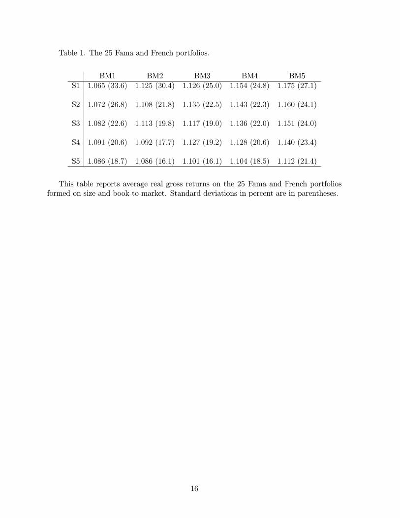
Table 1. The 25 Fama and French portfolios.
BM1 BM2 BM3 BM4 BM5S1 1:065 (33:6) 1:125 (30:4) 1:126 (25:0) 1:154 (24:8) 1:175 (27:1)
S2 1:072 (26:8) 1:108 (21:8) 1:135 (22:5) 1:143 (22:3) 1:160 (24:1)
S3 1:082 (22:6) 1:113 (19:8) 1:117 (19:0) 1:136 (22:0) 1:151 (24:0)
S4 1:091 (20:6) 1:092 (17:7) 1:127 (19:2) 1:128 (20:6) 1:140 (23:4)
S5 1:086 (18:7) 1:086 (16:1) 1:101 (16:1) 1:104 (18:5) 1:112 (21:4)
This table reports average real gross returns on the 25 Fama and French portfoliosformed on size and book-to-market. Standard deviations in percent are in parentheses.
16
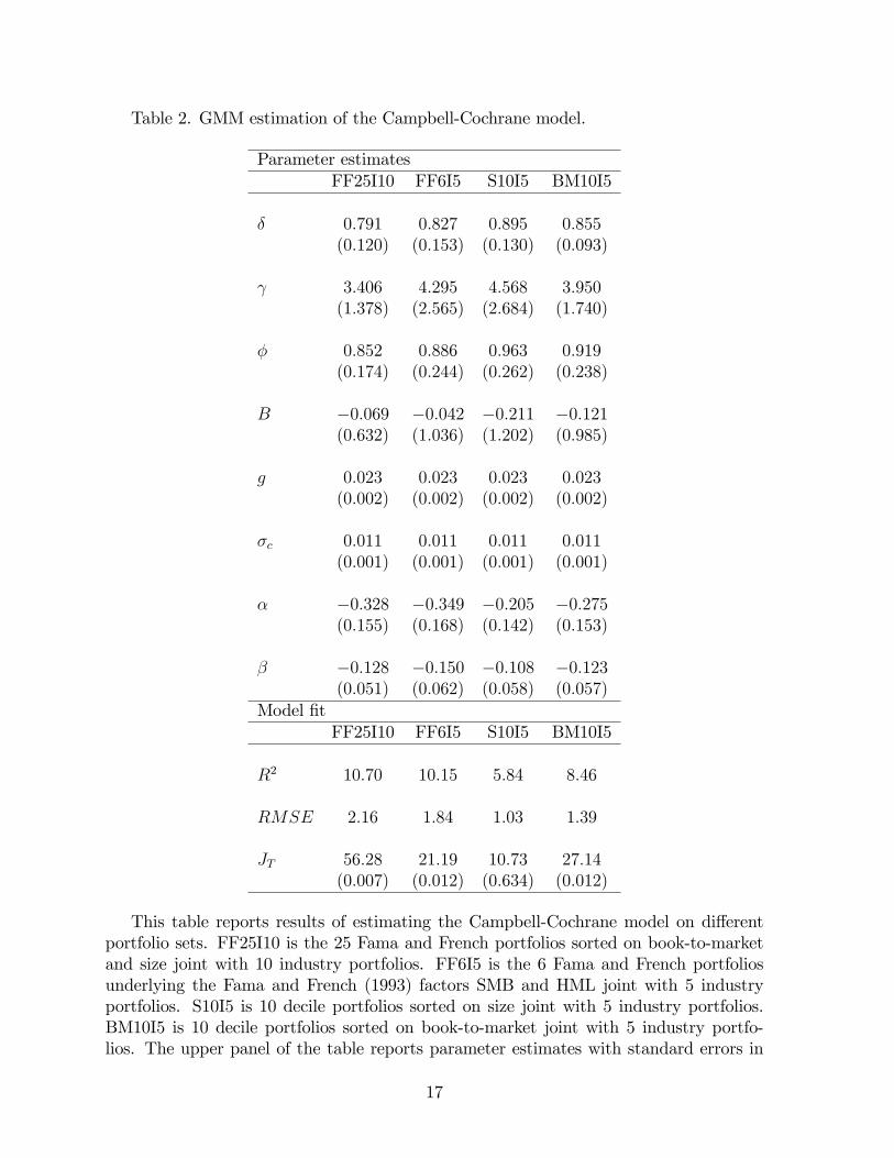
Table 2. GMM estimation of the Campbell-Cochrane model.
Parameter estimatesFF25I10 FF6I5 S10I5 BM10I5
� 0:791 0:827 0:895 0:855(0:120) (0:153) (0:130) (0:093)
3:406 4:295 4:568 3:950(1:378) (2:565) (2:684) (1:740)
� 0:852 0:886 0:963 0:919(0:174) (0:244) (0:262) (0:238)
B �0:069 �0:042 �0:211 �0:121(0:632) (1:036) (1:202) (0:985)
g 0:023 0:023 0:023 0:023(0:002) (0:002) (0:002) (0:002)
�c 0:011 0:011 0:011 0:011(0:001) (0:001) (0:001) (0:001)
� �0:328 �0:349 �0:205 �0:275(0:155) (0:168) (0:142) (0:153)
� �0:128 �0:150 �0:108 �0:123(0:051) (0:062) (0:058) (0:057)
Model �tFF25I10 FF6I5 S10I5 BM10I5
R2 10:70 10:15 5:84 8:46
RMSE 2:16 1:84 1:03 1:39
JT 56:28 21:19 10:73 27:14(0:007) (0:012) (0:634) (0:012)
This table reports results of estimating the Campbell-Cochrane model on di¤erentportfolio sets. FF25I10 is the 25 Fama and French portfolios sorted on book-to-marketand size joint with 10 industry portfolios. FF6I5 is the 6 Fama and French portfoliosunderlying the Fama and French (1993) factors SMB and HML joint with 5 industryportfolios. S10I5 is 10 decile portfolios sorted on size joint with 5 industry portfolios.BM10I5 is 10 decile portfolios sorted on book-to-market joint with 5 industry portfo-lios. The upper panel of the table reports parameter estimates with standard errors in
17

parentheses. The lower panel of the table reports measures of model �t. JT is Hansen�s(1982) test of overidentifying restrictions calculated as in (19). P-values are in parenthe-ses. RMSE is the root mean squared error calculated as in (20). R2 is the explanatorypower calculated as in (21) :
18
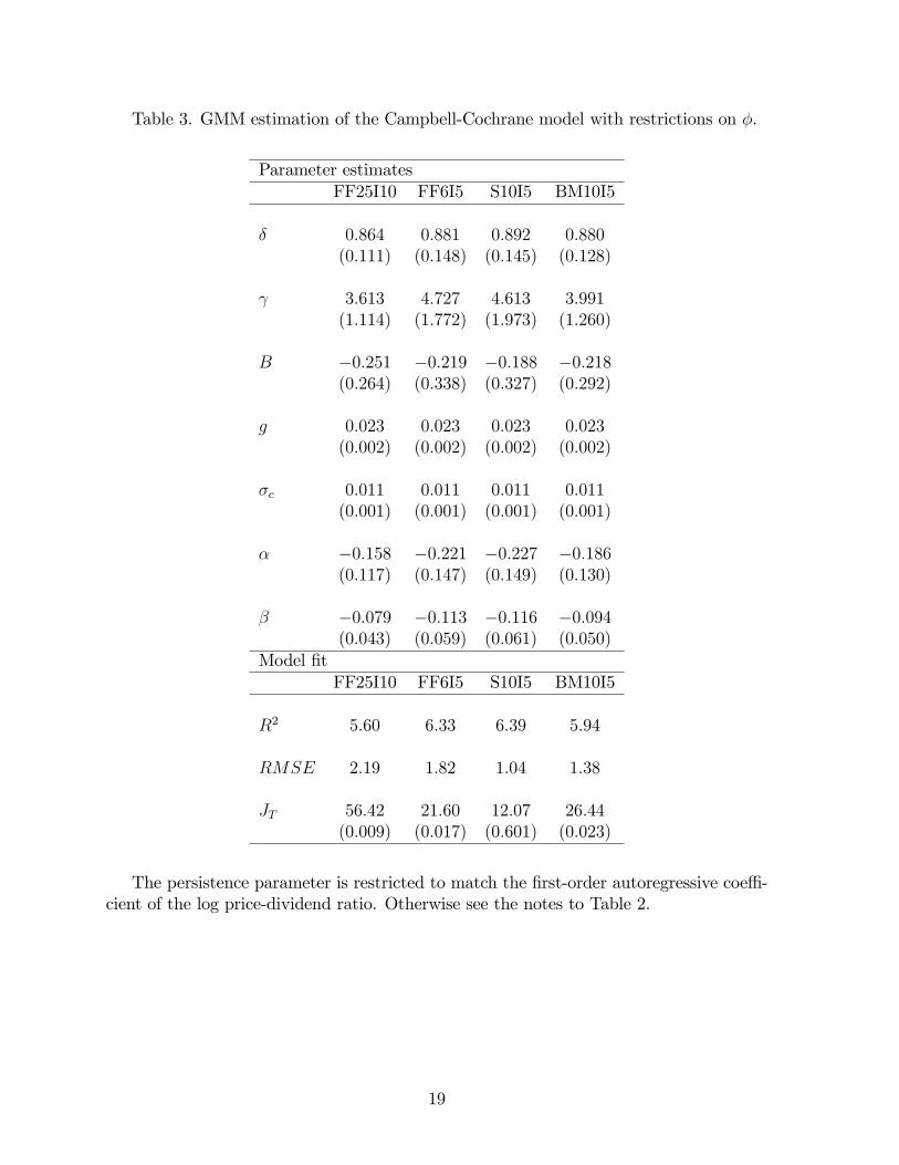
Table 3. GMM estimation of the Campbell-Cochrane model with restrictions on �.
Parameter estimatesFF25I10 FF6I5 S10I5 BM10I5
� 0:864 0:881 0:892 0:880(0:111) (0:148) (0:145) (0:128)
3:613 4:727 4:613 3:991(1:114) (1:772) (1:973) (1:260)
B �0:251 �0:219 �0:188 �0:218(0:264) (0:338) (0:327) (0:292)
g 0:023 0:023 0:023 0:023(0:002) (0:002) (0:002) (0:002)
�c 0:011 0:011 0:011 0:011(0:001) (0:001) (0:001) (0:001)
� �0:158 �0:221 �0:227 �0:186(0:117) (0:147) (0:149) (0:130)
� �0:079 �0:113 �0:116 �0:094(0:043) (0:059) (0:061) (0:050)
Model �tFF25I10 FF6I5 S10I5 BM10I5
R2 5:60 6:33 6:39 5:94
RMSE 2:19 1:82 1:04 1:38
JT 56:42 21:60 12:07 26:44(0:009) (0:017) (0:601) (0:023)
The persistence parameter is restricted to match the �rst-order autoregressive coe¢ -cient of the log price-dividend ratio. Otherwise see the notes to Table 2.
19
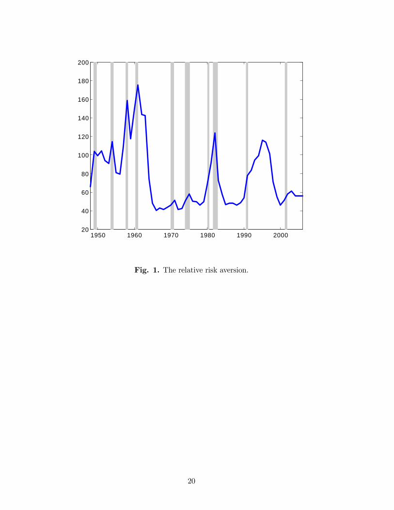
1950 1960 1970 1980 1990 200020
40
60
80
100
120
140
160
180
200
Fig. 1. The relative risk aversion.
20
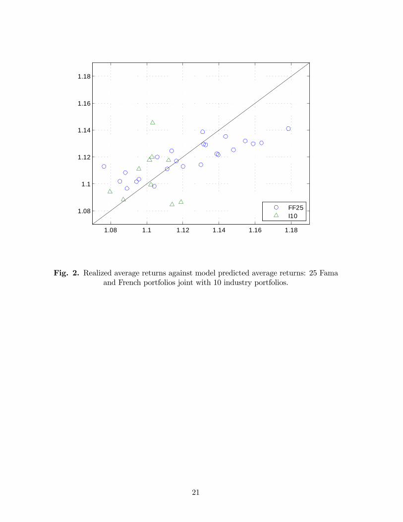
1.08 1.1 1.12 1.14 1.16 1.18
1.08
1.1
1.12
1.14
1.16
1.18
FF25I10
Fig. 2. Realized average returns against model predicted average returns: 25 Famaand French portfolios joint with 10 industry portfolios.
21
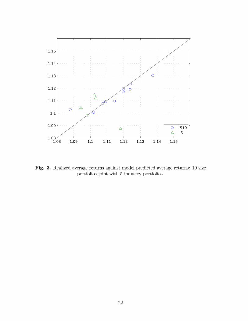
1.08 1.09 1.1 1.11 1.12 1.13 1.14 1.151.08
1.09
1.1
1.11
1.12
1.13
1.14
1.15
S10I5
Fig. 3. Realized average returns against model predicted average returns: 10 sizeportfolios joint with 5 industry portfolios.
22
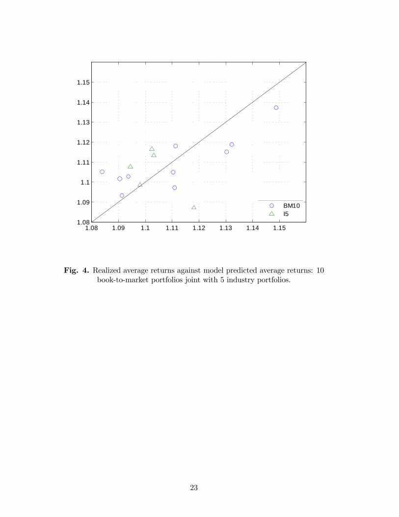
1.08 1.09 1.1 1.11 1.12 1.13 1.14 1.151.08
1.09
1.1
1.11
1.12
1.13
1.14
1.15
BM10I5
Fig. 4. Realized average returns against model predicted average returns: 10book-to-market portfolios joint with 5 industry portfolios.
23
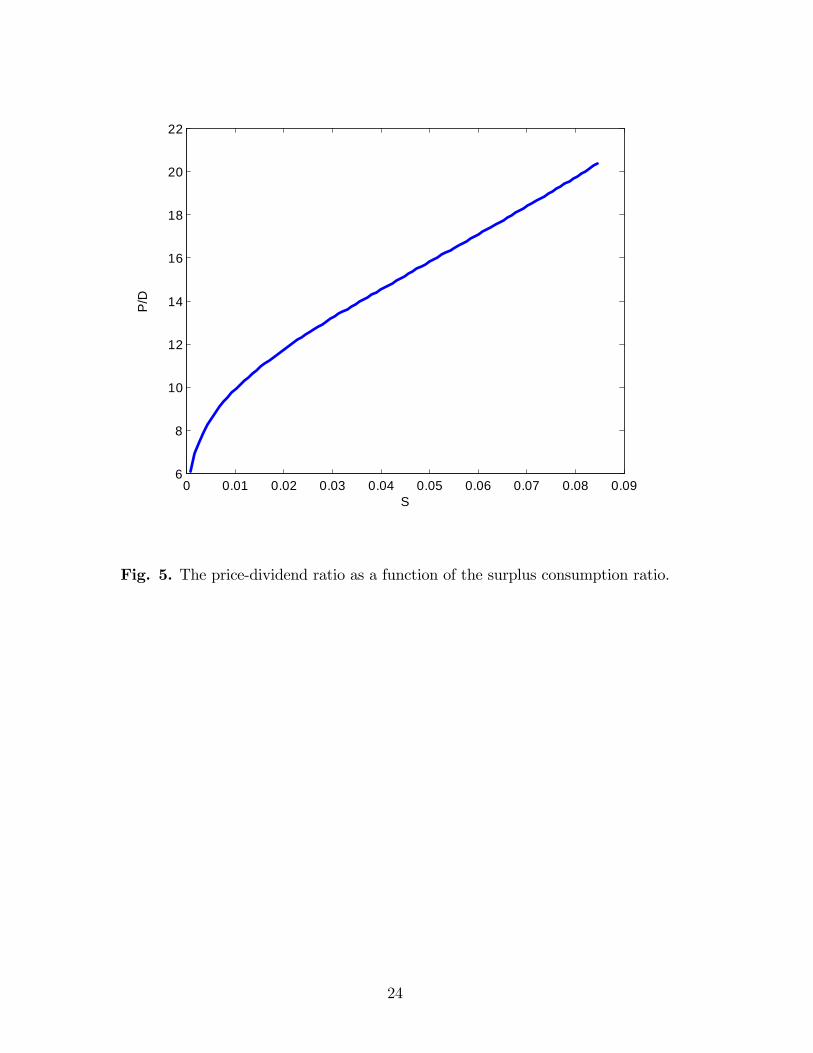
0 0.01 0.02 0.03 0.04 0.05 0.06 0.07 0.08 0.096
8
10
12
14
16
18
20
22
S
P/D
Fig. 5. The price-dividend ratio as a function of the surplus consumption ratio.
24
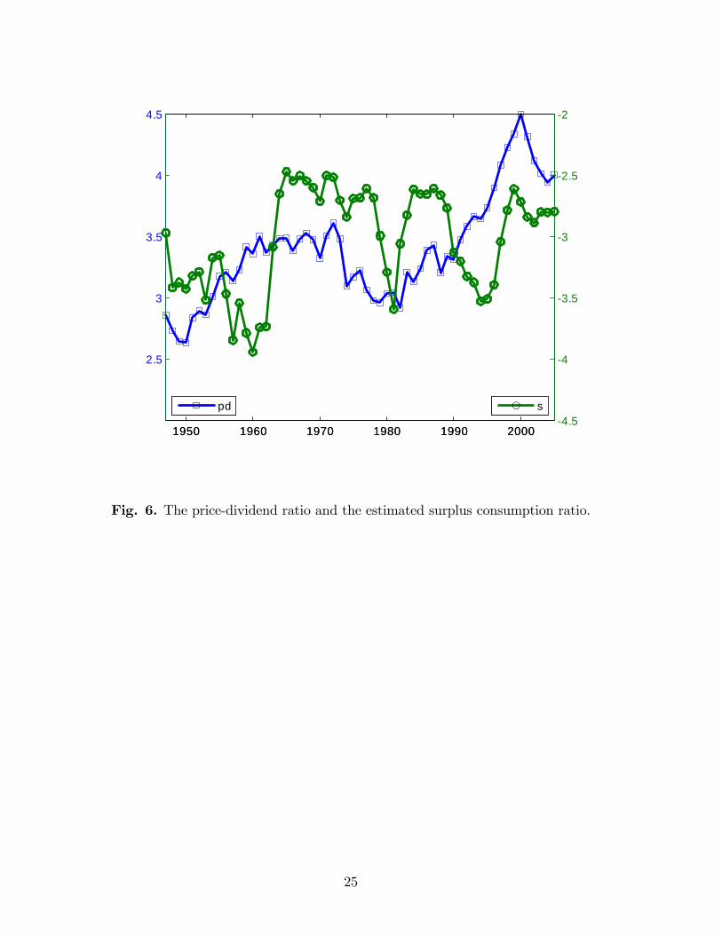
1950 1960 1970 1980 1990 2000
2.5
3
3.5
4
4.5
1950 1960 1970 1980 1990 2000-4.5
-4
-3.5
-3
-2.5
-2
spd
Fig. 6. The price-dividend ratio and the estimated surplus consumption ratio.
25

Chapter 3
Habit formation, surplus consumption and return predictability:International evidence
Habit formation, surplus consumption and returnpredictability: International evidence�
Tom Engstedy Stuart Hydez Stig Vinther Møllerx
Abstract
On an international post World War II dataset, we use an iterated GMM pro-cedure to estimate and test the Campbell-Cochrane (1999) habit formation modelwith a time-varying risk-free rate. In addition, we analyze the predictive powerof the surplus consumption ratio for future stock and bond returns. We �nd that,although there are important cross-country di¤erences and economically signi�cantpricing errors, for the majority of countries in our sample the model gets empiri-cal support in a variety of di¤erent dimensions, including reasonable estimates ofrisk-free rates. Further, for the majority of countries the surplus consumption ra-tio captures time-variation in expected returns. Together with the price-dividendratio, the surplus consumption ratio contains signi�cant information about futurestock returns, also during the 1990s. In addition, in most countries the surplusconsumption ratio is also a powerful predictor of future bond returns. Thus, thesurplus consumption ratio captures time-varying expected returns in both stockand bond markets.
JEL Classi�cation: E21, G12, G15Keywords: Habit formation, Campbell-Cochrane model, surplus consumptionratio, GMM estimation, pricing errors, return predictability.
�The �rst and third author acknowledge support from CREATES (Center for Research in Econo-metric Analysis of Time Series), funded by the Danish National Research Foundation. Comments andsuggestions from Belén Nieto, seminar participants at CREATES, and participants at the EFMA AnnualCongress in Athens, are gratefully acknowledged.
yCREATES, School of Economics and Management, University of Aarhus, Building 1322, DK-8000Aarhus C, Denmark. E-mail: [email protected].
zManchester Business School, University of Manchester, Crawford House, Booth Street East,Manchester, UK, M13 9PL. E-mail: [email protected].
xAarhus School of Business, University of Aarhus, Fuglesangs allé 4, DK-8210 Aarhus V., Denmarkand CREATES. E-mail: [email protected].

1 Introduction
Rumors of the death of the consumption based capital asset pricing model (C-CAPM)have been widely exaggerated. Throughout the 1980s asset pricing tests of the timeseparable power utility model provided direct evidence against the ability of the modelto capture the behavior of asset returns, although initially Hansen and Singleton (1982)reported results favorable to the model. Indeed, Mehra and Prescott (1985) demonstratedthat the return on US equity in excess of the risk-free rate is greater than that whichcan be explained by the standard consumption based model with a reasonable degreeof risk aversion. Lund and Engsted (1996) reported evidence against the standard C-CAPM for a number of European countries. However, the development of alternativeapproaches which either relax the assumption of separation between states (Epstein andZin, 1989, 1991) or abandon the time-separability constraint allowing habit formation(Abel, 1990; Constantinides, 1990; Campbell and Cochrane, 1999) breathed new life intothe consumption based framework. Subsequent empirical tests have proved to be moresupportive, resuscitating the C-CAPM, and leading Chen and Ludvigson (2006) to arguethat within the equilibrium consumption based framework, habit formation models arethe most promising and successful in describing aggregate stock market behavior.
In this paper we provide fresh international evidence on the pricing and predictabilityof asset returns. We investigate the performance of the Campbell and Cochrane (1999)habit formation speci�cation compared to the benchmark time-separable power utilitymodel. By adding the surplus consumption ratio to the standard C-CAPM with powerutility, Campbell and Cochrane show by calibration that their habit formation modelaccounts for a number of stylized facts on the US stock market, including time-varyingexpected returns. The model implies that individuals slowly develop habits for high orlow consumption such that the price of risk (risk aversion) becomes time-varying andcounter-cyclical: when consumption is well above habit in cyclical upswings, the priceof risk is low leading to low expected returns and high asset prices. In contrast, whenconsumption is close to habit, the price of risk is high leading to high expected returns andlow asset prices. However, there is scant evidence using non-US data on the performanceof the Campbell-Cochrane model.1 Indeed, even with US data many studies employ thecalibrated values from the original study rather than re-estimating and testing the modelempirically.2 We address this lack of international evidence by estimating the Campbell-Cochrane model using a post World War II sample of eight countries.3 Following thesuggested extension in Wachter (2006), we allow for cyclical variation in expected returnson bonds as well as stocks. We use an iterated GMM approach where, in each iteration,
1Engsted and Møller (2008) estimate the Campbell-Cochrane model on Danish data. However, otherinternational evidence (Hyde and Sherif, 2005; Hyde, Cuthbertson and Nitzsche, 2005; Li and Zhong,2005) employs US calibrated values when applying the model to non-US samples.
2For example, Li (2001, 2005) employs the calibrated values rather than estimating the parametersof the model. Tallarini and Zhang (2005), Fillat and Garduño (2005), Garcia, Renault and Semenov(2005) estimate the model with limited success while Møller (2008) estimates and reports supportiveevidence for the speci�cation.
3We assume that the national economies are closed, whereas Li and Zhong (2005) examine habitformation models in the context of world market integration.
1
a new time series for the surplus consumption ratio is generated, which is then used toobtain the moment conditions of the model. We �nd that, although there are importantcross-country di¤erences and economically signi�cant pricing errors, for the majority ofcountries in our sample the Campbell-Cochrane model is not rejected statistically andproduces economically plausible parameter values, including reasonable values for therisk-free rate.
Next, using the same international sample, we provide evidence on the power of thesurplus consumption ratio as a predictor for returns. It is a well established fact ofempirical �nance that stock returns are predictable. Evidence that aggregate valuationratios such as the price-dividend ratio and price-earnings ratio or �nancial/monetaryvariables such as the term spread or relative interest rate can account for the time-variation in expected returns is provided by Fama and French (1988, 1989), Campbell andShiller (1988a, 1988b), Campbell (1991) and Hodrick (1992). However, the documentedinability of the price-dividend ratio to capture time-variation in expected returns duringthe 1990s has resulted in the emergence of a number of new predictor variables. Forinstance, Boudoukh et al. (2007) argue that the net payout ratio is more appropriatethan the price-dividend ratio since it captures more accurately the extent of distributingcash to shareholders and show that it has greater ability to predict future returns.
Alternatively, many of these new predictors are linked to macroeconomic factors suchas consumption, labor income, and output demonstrating the strong links between the�nancial and real sectors of the economy. From the representative consumer�s budgetconstraint, Lettau and Ludvigson (2001a, 2001b) show that the consumption-wealthratio, cay, contains information about future returns.4 Further, Santos and Veronesi(2006) introduce a labor income-consumption ratio which predicts US returns well bothindependently and in addition to the price-dividend ratio. Julliard (2007) argues that theconsumption-wealth ratio should be combined with expected future labor income growthto predict future US returns, demonstrating not only that expected changes in laborincome have high predictive power for future returns but that together the consumption-wealth ratio and expected changes in labor income explain much of the variation inthe cross-section of returns. Using the calibrated parameter values from Campbell andCochrane (1999), Li (2005) examines the forecasting power of the surplus consumptionratio in addition to the consumption-wealth ratio for US stock returns, documentingthat the surplus consumption ratio contains incremental information not incorporatedin the consumption-wealth ratio. Additionally, Møller (2008) provides evidence thatthe estimated surplus consumption ratio has strong predictive abilities. Focusing onoutput rather than consumption, Rangvid (2006) advocates the adoption of a price-output variable and provides evidence that it explains more of the time-variation inexpected returns than either the price-earnings or price-dividend ratios and performs aswell as cay for US returns. Rangvid (2006) also provides evidence on an internationalsample, showing that the ability of the price-output ratio to predict returns is robustoutside the US.
4The consumption-wealth ratio is measured as the residuals of the cointegrating relationship betweenlog consumption, log asset wealth and log labor income.
2
Time-varying expected returns have also been documented on the bond market. Famaand Bliss (1987), Fama and French (1989), Campbell and Shiller (1991), and Cochraneand Piazzesi (2005) �nd that excess bond returns are forecastable by �nancial variablessuch as forward spreads and term spreads. New work by Ludvigson and Ng (2007) linktime-varying expected bond returns together with macroeconomics. They form macrofactors based on principal components of a large number of macroeconomic series and�nd that these macro factors predict counter-cyclical movements in excess bond returns.Buraschi and Jiltsov (2007) also develop a model which links bond returns with un-derlying macro factors, allowing for time-variation in interest rates. They highlight theability of habit formation to describe important characteristics of the US nominal termstructure.
Here we examine bond and stock return predictability using annual data over thepost World War II period up to 2004. Given the debate regarding disappearing pre-dictability in the 1990s we also report results for a shorter sample that ends in 1990.We demonstrate that the surplus consumption ratio signi�cantly predicts future stockreturns in the majority of countries. To check the robustness of this result we examinebivariate regressions with alternative predictors. We consider two of the traditional re-turn predictors; the price-dividend ratio and the term spread. We show that the abilityof the surplus consumption ratio to predict future returns is not diminished by includingthese additional predictors. In particular, the surplus consumption ratio together withthe price-dividend ratio contains signi�cant information about future stock returns inmost countries and, interestingly, the predictive power remains statistically signi�cantduring the 1990s. Furthermore, the surplus consumption ratio is shown to be a powerfulpredictor of future bond returns in most countries. This is also robust to the inclusionof alternative predictor variables. Our �ndings therefore support the extended versionof the Campbell-Cochrane model in which expected returns on stocks and bonds movecounter-cyclically with the surplus consumption ratio. In general, the countries in whichthe surplus consumption ratio is a useful return predictor are the same that get mostempirical support in the GMM estimations. Thus, our analysis implies that, althoughthere are clear cross-country di¤erences, for many countries several of the implicationsof the Campbell-Cochrane model are supported empirically.
The remainder of the paper is set out as follows. Section 2 describes the consumptionbased asset pricing models. Section 3 provides details on the GMM estimation of themodels while section 4 gives details of the data and section 5 reports the empirical results.Section 6 concludes.
2 The models
In the consumption based asset pricing framework the representative agent makes con-sumption and investment decisions in order to maximize expected lifetime utility. Thismaximization problem implies the following �rst order condition that all correctly priced
3
assets must satisfy:Et [Ri;t+1Mt+1] = 1: (1)
Ri;t+1 is the real gross return of investing in asset i at time t and selling it at time t+ 1,and Mt+1 is the stochastic discount factor:
Mt+1 = �U 0 (Ct+1)
U 0 (Ct); (2)
where � is the subjective time discount factor, Ct is real consumption, and U 0 (�) ismarginal utility. To observe the stochastic discount factor the representative agent�sutility function has to be speci�ed. With standard CRRA utility,
U (Ct) =C1� t � 11� ; (3)
where is the coe¢ cient of relative risk aversion, the stochastic discount factor equals:
Mt+1 = �
�Ct+1Ct
�� : (4)
Inserting (4) in (1), the log expected excess return can be stated approximately as:
Et�ri;t+1
�� rf;t+1 +
1
2�2i;t = Covt
�ri;t+1; log
�Ct+1Ct
��; (5)
where ri;t+1 � log (Ri;t+1), �2i;t is the variance of ri;t, and rf;t+1 is the log risk-free rate.
Empirically the consumption based CRRA model has run into trouble because thecovariance between stock returns and consumption growth is too low to explain thehistorically high excess return on stocks, unless the degree of risk aversion is extremelyhigh. In addition, even if an extremely high value of is accepted, it would imply animplausibly high real risk-free rate. Assuming that returns and consumption growth areiid and jointly lognormally distributed, the log real risk-free rate is:
rf;t+1 = � log (�) + g �1
2 2�2c ; (6)
where g and �2c are mean and variance of consumption growth. Thus, the real risk-freerate is very sensitive to the mean consumption growth rate for high values of . Con-sequently, the standard speci�cation cannot solve the equity premium puzzle withoutrunning into a risk-free rate puzzle. Furthermore, the CRRA model also faces a returnpredictability puzzle since the consumption covariance with returns is too smooth to ac-count for time-variation in expected returns, cf. Ferson and Harvey (1993), Li (2001)among others. New consumption based models have been developed to solve these puz-zles. In what follows we present the habit persistence model of Campbell and Cochrane(1999) with the extension suggested by Wachter (2006) to allow for a time-varying risk-free rate in order to generate a nontrivial term structure.5
5The working paper version of Campbell and Cochrane (1999) [Campbell and Cochrane (1995)] alsocontains an analysis with a time-varying risk-free rate.
4

The utility function in the Campbell-Cochrane model is speci�ed as follows:
U(Ct; Xt) =(Ct �Xt)
1� � 11� ; Ct > Xt; (7)
where Xt is an external habit level of consumption. With this speci�cation the surplusconsumption ratio, St = Ct�Xt
Ct, becomes a business cycle variable that is high in cyclical
upswings and low in cyclical downturns such that relative risk aversion, =St, movescounter-cyclically. Rather than specifying a process for the habit, Xt, Campbell andCochrane specify a process for the log surplus consumption ratio, st = log (St), to ensurethat consumption is above habit at all times. The log surplus consumption ratio ismodeled as a stationary �rst-order autoregressive process:
st+1 = (1� �) �s+ �st + � (st) vt+1; (8)
where 0 < � < 1 is the habit persistence parameter, �s is the steady state level of st, and� (st) is the sensitivity function that determines how innovations in consumption growthvt+1 in�uence st+1. The consumption growth process is given by:
4ct+1 = g + vt+1; vt+1 � niid�0; �2c
�; (9)
where ct = log (Ct), and g is the mean consumption growth rate, as in (6). The sensitivityfunction �(st) is speci�ed as follows:
� (st) =
( 1�S
p1� 2 (st � �s)� 1 if st � smax
0 otherwise
); (10)
where
S =
s�2c
1� ��B= ; smax = s+1
2(1� S2); s = log(S):
Specifying � (st) in this way implies that the real risk-free rate is a linear function of st.Using the stochastic discount factor,
Mt+1 = �
�St+1St
Ct+1Ct
�� ; (11)
the log real risk-free rate can be derived as:
rf;t+1 = r �Bset ; (12)
where set = (st � s) and r = � log (�) + g � (1��)�B
2is the average real risk-free rate.
B governs the cyclicality of real risk-free rates; if B > 0, the real risk-free rate movescounter-cyclically; if B < 0, the real risk-free rate moves pro-cyclically; and if B = 0,we obtain the baseline Campbell-Cochrane model with a constant real risk-free rate.
The log expected excess return is given by the following:
Et�ri;t+1
�� rf;t+1 +
1
2�2i;t = [1 + � (st)]Covt
�ri;t+1; log
�Ct+1Ct
��; (13)
5
which states that expected excess returns move counter-cyclically with st since � (st)is decreasing in st. When surplus consumption falls in cyclical downturns, investorsrequire a higher expected return and vice versa. Thus, in contrast to the CRRA model,the Campbell-Cochrane model accounts for counter-cyclical time-variation in expectedreturns despite smooth consumption covariance with returns.
Campbell and Cochrane (1999) calibrate their model with a constant risk-free rate(i.e. B = 0) by choosing parameter values to match certain moments of postwar USdata. They �nd that the model explains a number of stylized facts for the US stockmarket, including stock return predictability. Wachter (2006) also calibrates the modelby matching certain moments of postwar US data, but now with a time-varying risk-freerate (i.e. B 6= 0). Her focus is on explaining nominal bond yields, and she �nds thatthe model accounts for many of the observed features of the term structure of interestrates. Instead of doing such calibration exercises, we use an iterated GMM approach toestimate all the parameters of the model. In the next section we describe the econometricapproach.
3 GMM estimation of the models
We estimate the CRRA model and the Campbell-Cochrane model using the GMM tech-nique of Hansen (1982). From the �rst order condition (1), we estimate the CRRA modelbased on the following moment conditions:
0 = E
" (RS;t+1 �Rf;t+1)
�Ct+1Ct
�� !Zt
#; (14)
0 = E
" (RLB;t+1 �Rf;t+1)
�Ct+1Ct
�� !Zt
#; (15)
0 = E
" (Rf;t+1) �
�Ct+1Ct
�� � 1!Zt
#: (16)
RS;t+1 is the real gross returns on stocks, RLB;t+1 is the real gross return on long-termbonds, and Rf;t+1 is the real risk-free rate proxied by the real gross return on 3-monthT-bills, i.e. the test assets in (14) to (16) are the excess stock return, the excess bondreturn, and the ex post real T-bill rate. Following Kocherlakota (1996), among others,we include a moment condition for the real T-bill rate as well as the excess stock returnin order to focus on both the equity premium puzzle and the risk-free rate puzzle. Sincethe expectation in (1) is conditional on information available at time t, we use a vector ofinstruments Zt observable at time t to capture the relevant conditioning information. Inaddition to a constant, the instrument vector Zt contains the log price-dividend ratio.6
6Campbell and Shiller (1988b) and Fama and French (1988, 1989) document that the price-dividendratio is a strong return predictor, suggesting that the price-dividend ratio is a useful instrument inthe GMM estimations. We have also used an expanded set of instruments, but in general di¤erentcombinations of instruments do not change the main results.
6

De�ning gT (�CRRA) as the sample moment conditions of (14) to (16) based on T obser-vations, we estimate the parameter vector �CRRA = (�; )
0 by minimizing the quadraticform, gT (�CRRA)
0WgT (�CRRA), where W is a positive de�nite weighting matrix. Asweighting matrix, W , we use the identity matrix, I, to give equal weight to all momentconditions, following Cochrane�s (2005) suggestion.
The Campbell-Cochrane model is estimated based on the following moment condi-tions:
0 = E
" (RS;t+1 �Rf;t+1)
�St+1St
Ct+1Ct
�� !Zt
#; (17)
0 = E
" (RLB;t+1 �Rf;t+1)
�St+1St
Ct+1Ct
�� !Zt
#; (18)
0 = E
��rf;t+1 �
�� log (�) + g � (1� �)�B
2
�+Bset
�(1 set)
0�; (19)
0 = E [4ct+1 � g] ; (20)
0 = E�(4ct+1 � g)2 � �2c
�; (21)
0 = E�(pdt+1 � �� �pdt) (1 pdt)
0� : (22)
As for the CRRA model, we estimate the Campbell-Cochrane model using the excessstock return, the excess bond return, and the real T-bill rate as test assets, which leadsto the moment conditions in (17), (18), and (19). Following the speci�cation in (12), themoment conditions in (19) impose the restriction that the average log real risk-free rateis given by r = � log (�) + g � (1��)�B
2. From the random walk model of consumption
in (9), we obtain the moment conditions in (20) and (21). Since consumption follows arandom walk, the natural choice of instruments is a constant only. Following Campbelland Cochrane (1999) and Wachter (2006), we estimate the persistence parameter, �,as the �rst-order autoregressive coe¢ cient of the log price-dividend ratio, pdt, whichleads to the moment conditions in (22). This is feasible since in the model the surplusconsumption ratio is the only state variable, whereby the price-dividend ratio inheritsthe dynamic properties from the surplus consumption ratio.
The estimation of the Campbell-Cochrane model is complicated by the fact that thesurplus consumption ratio is not observable in the same way as returns and consumptionare directly observable. To observe the st process, we use s0 = s as starting value of st att = 0. Then we choose starting values of the model parameters and obtain the st processrecursively using (8).7 We use an iterated GMM approach where, in each iteration, a newtime series for the surplus consumption ratio is generated, which is then used to obtainthe moment conditions of the model. The iterations are continued until convergence ofall model parameters.
De�ning gT (�CC) as the sample moment conditions based on T observations, theparameter vector �CC = (�; ; g; �2c ; �; �;B)
0 is estimated by minimizing the quadratic
7We use the calibrated parameter values in Campbell and Cochrane (1999) as starting values.
7
form, gT (�CC)0WgT (�CC). As for the CRRA model, we use the identity matrix as
weighting matrix to give equal weight to all moment conditions.
The use of a �xed and model-independent weighting matrix such as the identitymatrix allows us to compare the magnitude of the estimated pricing errors across di¤erentmodels. Since the chosen weighting matrix is not the e¢ cient Hansen (1982) matrix butthe identity matrix, I, the formula for the covariance matrix of the parameter vector is(cf. Cochrane (2005), chpt. 11):
V ar(b�) = 1
T(d0Id)�1d0ISId(d0Id)�1; (23)
where d = @gT (�)=@�0, and the spectral density matrix S =P1
j=�1E[ gT (�)gT�j(�)0] is
estimated using the Newey and West (1987) estimator with a Bartlett kernel. To evaluatethe model �t we use Hansen�s J-test of overidentifying restrictions:
JT = TgT (b�)0 hV ar(gT (b�))i�1 gT (b�); (24)
where V ar(gT (b�)) = 1T(I�d(d0Id)�1d0I)S(I�d(d0Id)�1d0I)0 is singular and hence inverted
using the Moore-Penrose pseudo-inversion. JT has an asymptotic �2 distribution withdegrees of freedom equal to the number of moment conditions minus the number ofparameters.
The J-test provides a statistical test whether the moment conditions for a given modelare signi�cantly di¤erent from zero. As a supplement to the J-test we use Hansen andJagannathan�s (1997) distance measure that provides a useful economic measure of themodel �t. The Hansen-Jagannathan distance is given by:
HJ =�E(Mt+1(�)Rt+1 � 1)0(E(Rt+1R0t+1))�1E(Mt+1(�)Rt+1 � 1)
� 12 : (25)
HJ gives the minimum distance from the stochastic discount factor of a given model tothe set of true stochastic discount factors that price assets correctly. It is a measure ofthe maximum percentage pricing error associated with a given model and hence gives acomparable measure of model misspeci�cation.
4 Data and summary statistics
We study the following eight countries: Belgium, Canada, France, Germany, Italy, Swe-den, the UK, and the US. We select these countries on the basis of data availability. Oursamples of annual observations begin between 1949 and 1953, depending on the country,and end in 2004. We measure consumption as private total consumption from IMF Inter-national Financial Statistics and adopt the Campbell (2003) beginning of period timingassumption that consumption during year t takes place at the beginning of year t. Nom-inal consumption is converted to real units using the consumer prices indices from IMFInternational Financial Statistics. Real per capita consumption is constructed using the
8
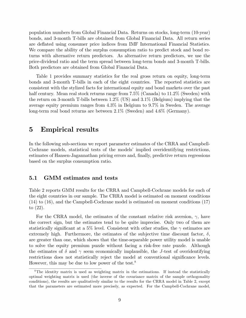
population numbers from Global Financial Data. Returns on stocks, long-term (10-year)bonds, and 3-month T-bills are obtained from Global Financial Data. All return seriesare de�ated using consumer price indices from IMF International Financial Statistics.We compare the ability of the surplus consumption ratio to predict stock and bond re-turns with alternative return predictors. As alternative return predictors, we use theprice-dividend ratio and the term spread between long-term bonds and 3-month T-bills.Both predictors are obtained from Global Financial Data.
Table 1 provides summary statistics for the real gross return on equity, long-termbonds and 3-month T-bills in each of the eight countries. The reported statistics areconsistent with the stylized facts for international equity and bond markets over the pasthalf century. Mean real stock returns range from 7.5% (Canada) to 11.2% (Sweden) withthe return on 3-month T-bills between 1.2% (US) and 3.1% (Belgium) implying that theaverage equity premium ranges from 4.3% in Belgium to 9.7% in Sweden. The averagelong-term real bond returns are between 2.1% (Sweden) and 4.6% (Germany).
5 Empirical results
In the following sub-sections we report parameter estimates of the CRRA and Campbell-Cochrane models, statistical tests of the models� implied overidentifying restrictions,estimates of Hansen-Jagannathan pricing errors and, �nally, predictive return regressionsbased on the surplus consumption ratio.
5.1 GMM estimates and tests
Table 2 reports GMM results for the CRRA and Campbell-Cochrane models for each ofthe eight countries in our sample. The CRRA model is estimated on moment conditions(14) to (16), and the Campbell-Cochrane model is estimated on moment conditions (17)to (22).
For the CRRA model, the estimates of the constant relative risk aversion, , havethe correct sign, but the estimates tend to be quite imprecise. Only two of them arestatistically signi�cant at a 5% level. Consistent with other studies, the estimates areextremely high. Furthermore, the estimates of the subjective time discount factor, �,are greater than one, which shows that the time-separable power utility model is unableto solve the equity premium puzzle without facing a risk-free rate puzzle. Althoughthe estimates of � and seem economically implausible, the J-test of overidentifyingrestrictions does not statistically reject the model at conventional signi�cance levels.However, this may be due to low power of the test.8
8The identity matrix is used as weighting matrix in the estimations. If instead the statisticallyoptimal weighting matrix is used (the inverse of the covariance matrix of the sample orthogonalityconditions), the results are qualitatively similar to the results for the CRRA model in Table 2, exceptthat the parameters are estimated more precisely, as expected. For the Campbell-Cochrane model,
9

The Campbell-Cochrane model resembles the CRRAmodel in terms of an overall highlevel of relative risk aversion. The steady state relative risk aversion, = �S, varies acrosscountries from 25 in Belgium to 75 in France. Unlike the CRRA model, though, theCampbell-Cochrane model has the important ability to escape the risk-free rate puzzle.In fact, the estimates of the time discount factor, �, are less than 1 in all countries. Forsome countries, however, the � estimates seem too low to be economically reasonable;this is in particular the case for France. Despite the cross-country di¤erences, the J-testdoes not reject the Campbell-Cochrane model in any country. Again, this may be due tolow power of the test. The estimates of the persistence parameter, �, range from 0.74 inGermany to 0.95 in the US, implying highly persistent but stationary log price-dividendratio�s and, hence, surplus consumption ratio�s. The mean consumption growth rateranges from around 2% in most of the countries to around 3% in two of the countries.
Table 2 also reports the implied risk-free rate (rf) for the CRRA model, and the es-timated mean risk-free rate (r) and cyclicality parameter (B) in the Campbell-Cochranemodel. For the CRRA model the implied rf varies considerably across countries, rangingfrom �52:72% in Germany to 10:39% in Sweden. For the Campbell-Cochrane model,reasonable r values are obtained for all countries, ranging from 1:24% in the US to 3:00%in Belgium. Except for the UK, all B estimates are positive, implying a counter-cyclicalrisk-free rate, an upward-sloping yield curve, and positive bond risk-premia. Note, how-ever, that some of the B estimates are statistically insigni�cant, or only marginallysigni�cant.
Finally, Table 2 reports estimates of the Hansen and Jagannathan (1997) distancefor the CRRA and Campbell-Cochrane models using the preference parameter estimatesfrom the GMM estimation. The Hansen-Jagannathan distance provides the maximumpercentage pricing error associated with a given model and is suitable for direct modelcomparisons. The distances are estimated using the excess stock return, the excess bondreturn and the real T-bill rate. Although the J-test does not statistically reject themodels, the magnitude of the distances are economically signi�cant for both models.Moreover, the CRRA model has lower distances than the Campbell-Cochrane model.Since we use W = I and not W = E(Rt+1R
0t+1)
�1 as weighting matrix, we do notestimate the parameters of the models to minimize the Hansen-Jagannathan distance,but still it is surprising that the Campbell-Cochrane model performs worse than theCRRA model.
The evidence in this subsection gives mixed results regarding the consumption basedframework�s ability to explain international asset returns. The CRRA and Campbell-Cochrane models are not rejected statistically at conventional signi�cance levels, butthe Hansen-Jagannathan measure does indicate economically large pricing errors alsofor the Campbell-Cochrane model. In the remaining part of the paper we investigatethe Campbell-Cochrane model in another dimension, by analyzing whether the surplusconsumption ratio contains useful information about future returns.
using the statistically optimal weighting matrix does not lead to convergence with positive values of in the GMM iterations, a problem also faced by Garcia, Renault and Semenov (2005). Thus, we restrictattention to the case with W = I.
10
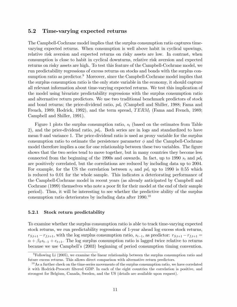
5.2 Time-varying expected returns
The Campbell-Cochrane model implies that the surplus consumption ratio captures time-varying expected returns. When consumption is well above habit in cyclical upswings,relative risk aversion and expected returns on risky assets are low. In contrast, whenconsumption is close to habit in cyclical downturns, relative risk aversion and expectedreturns on risky assets are high. To test this feature of the Campbell-Cochrane model, werun predictability regressions of excess returns on stocks and bonds with the surplus con-sumption ratio as predictor.9 Moreover, since the Campbell-Cochrane model implies thatthe surplus consumption ratio is the only state variable in the economy, it should captureall relevant information about time-varying expected returns. We test this implication ofthe model using bivariate predictability regressions with the surplus consumption ratioand alternative return predictors. We use two traditional benchmark predictors of stockand bond returns; the price-dividend ratio, pdt (Campbell and Shiller, 1988; Fama andFrench, 1989; Hodrick, 1992), and the term spread, TERMt (Fama and French, 1989;Campbell and Shiller, 1991).
Figure 1 plots the surplus consumption ratio, st (based on the estimates from Table2), and the price-dividend ratio, pdt. Both series are in logs and standardized to havemean 0 and variance 1. The price-dividend ratio is used as proxy variable for the surplusconsumption ratio to estimate the persistence parameter � and the Campbell-Cochranemodel therefore implies a one for one relationship between these two variables. The �gureshows that the two series tend to move together, but in many countries they become lessconnected from the beginning of the 1990s and onwards. In fact, up to 1990 st and pdtare positively correlated, but the correlations are reduced by including data up to 2004.For example, for the US the correlation between st and pdt up to 1990 is 0.55 whichis reduced to 0.01 for the whole sample. This indicates a deteriorating performance ofthe Campbell-Cochrane model in recent years (as already anticipated by Campbell andCochrane (1999) themselves who note a poor �t for their model at the end of their sampleperiod). Thus, it will be interesting to see whether the predictive ability of the surplusconsumption ratio deteriorates by including data after 1990.10
5.2.1 Stock return predictability
To examine whether the surplus consumption ratio is able to track time-varying expectedstock returns, we run predictability regressions of 1-year ahead log excess stock returns,rS;t+1� rf;t+1, with the log surplus consumption ratio, st�1, as predictor: rS;t+1� rf;t+1 =� + �Sst�1 + et+1. The log surplus consumption ratio is lagged twice relative to returnsbecause we use Campbell�s (2003) beginning of period consumption timing convention.
9Following Li (2005), we examine the linear relationship between the surplus consumption ratio andfuture excess returns. This allows direct comparison with alternative return predictors.10As a further check on the time-series movements of the surplus consumption ratio, we have correlated
it with Hodrick-Prescott �ltered GDP. In each of the eight countries the correlation is positive, andstrongest for Belgium, Canada, Sweden, and the US (details are available upon request).
11

Table 3 reports standard Newey and West (1987) corrected t-statistics and adjustedR2-statistics.11 The upper panel reports the full sample results up to 2004, and thelower panel reports the sub sample results up to 1990. Consistently with the Campbell-Cochrane model, the table shows that the surplus consumption ratio is negatively relatedto future excess stock returns, such that low surplus consumption ratio�s in cyclicaldownturns predict high future excess stock returns. However, the predictive power variesstrongly across countries. Based on the t-statistics and adjusted R2-statistics, there isstatistical evidence of stock return predictability in Belgium, Sweden, the UK, and theUS (and also France and Italy if the sample is restricted to end in 1990), but the surplusconsumption ratio has low predictive power in Canada and Germany.
Next, to compare the surplus consumption ratio�s predictive power for future stockreturns with alternative predictors, we use in turn the price-dividend ratio and the termspread in bivariate predictability regressions together with the surplus consumption ratio.Throughout the predicted variable is the 1-year ahead log excess stock return.
Table 4 shows that the surplus consumption ratio does not drive out the price-dividendratio in bivariate predictability regressions of future excess stock returns. In fact, theprice-dividend ratio is a signi�cant predictor in all countries except Germany. The surplusconsumption ratio remains a signi�cant predictor in Belgium, France, Italy, Sweden, andthe US, but is driven out as a signi�cant predictor in the UK. The overall conclusion isthat both predictors have signi�cant forecasting ability for future excess stock returns inthe majority of countries and, interestingly, they remain signi�cant when including datafrom the 1990s, which is surprising in light of the �ndings in other recent studies, e.g.Ang and Bekaert (2007).
Turning to bivariate predictability regressions of future stock returns with the surplusconsumption ratio and the term spread as predictors, Table 5 shows that the term spreaddoes not bring much additional information about future stock returns relative to thesurplus consumption ratio. The exception is Canada, but otherwise the term spread isnot signi�cant in bivariate predictability regressions with the surplus consumption ratio.
The overall impression from the results so far is that the surplus consumption ratiosigni�cantly captures time-varying expected stock returns to a greater or lesser extent inBelgium, France, Italy, Sweden, the UK, and the US, but not in Canada and Germany.Furthermore, the surplus consumption ratio appears to be a stronger stock return predic-tor than the term spread. However, the surplus consumption ratio does not consistentlydrive out the price-dividend ratio in bivariate predictability regressions, which suggeststhat the surplus consumption ratio does not capture all relevant information about futurestock returns.11Valkanov (2003) shows that the use of overlapping data in a small sample may lead to spurious
evidence of return predictability. By using only non-overlapping data we are less exposed to suchconcerns.
12

5.2.2 Bond return predictability
The basic version of the Campbell-Cochrane model does not generate time-varying ex-pected returns on bonds since bond returns at all maturities are equal to the constantrisk-free rate. However, our version of the model incorporates the extension suggested byWachter (2006) such that the surplus consumption ratio captures counter-cyclical time-variation in both stock and bond returns. We analyze this extended version of the modelby running predictability regressions of 1-year ahead log excess bond returns with the logsurplus consumption ratio as predictor. Table 6 shows that, indeed, high surplus con-sumption ratio�s predict low future excess bond returns. As with excess stock returns,the ratio signi�cantly predicts excess bond returns in Belgium, France, Italy, Sweden,the US, and to some extent the UK. Furthermore, the surplus consumption ratio alsopredicts excess bond returns in Canada. Once again, though, the surplus consumptionratio does not have predictive power in Germany.
Table 7 shows that the price-dividend ratio is generally not a signi�cant predictor ofexcess bond returns. It appears that the price-dividend ratio only predicts excess stockreturns, but not excess bond returns, whereas the surplus consumption ratio capturesa common source of predictability in both excess stock and bond returns. The mostoften used predictor for excess bond returns is the term spread. In Table 8 we includethis variable together with the surplus consumption ratio in bivariate predictability re-gressions. The table shows that the surplus consumption ratio is a better bond returnpredictor than the term spread for the majority of countries. The main exception isthe US, where the term spread seems to drive out the surplus consumption ratio as asigni�cant predictor.
There is growing body of literature about return predictability on both stocks andbonds. However, a common limitation to existing return predictors is that they only con-tain information about either future stock returns or future bond returns. Interestingly,we �nd that the surplus consumption ratio captures predictive patterns in both stockand bond markets. Our �ndings therefore support the extended version of the Campbell-Cochrane model in which expected returns on stocks and bonds move counter-cyclicallywith the surplus consumption ratio.
5.2.3 Small sample bias
As a �nal robustness check, we examine to what extent our results su¤er from small sam-ple bias. Stambaugh (1999) shows that standard OLS inference is biased in �nite sampleswhen the predictive variable is highly persistent and its innovations are correlated withthe innovations in returns. Amihud and Hurvich (2004) extend the work of Stambaugh(1999) by developing a straightforward estimation method to obtain bias-adjusted betaestimates and t-statistics. Tables 9 and 10 report the Amihud-Hurvich bias-adjustedresults using the surplus consumption ratio to predict excess stock and bond returns, re-
13
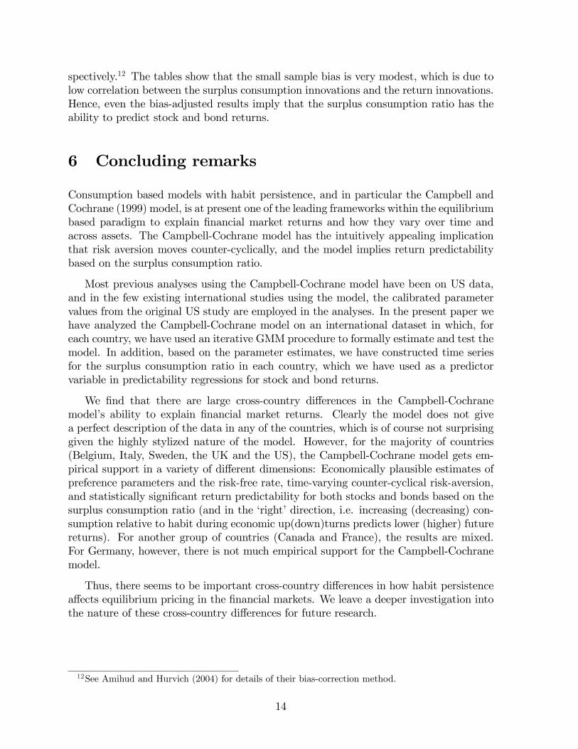
spectively.12 The tables show that the small sample bias is very modest, which is due tolow correlation between the surplus consumption innovations and the return innovations.Hence, even the bias-adjusted results imply that the surplus consumption ratio has theability to predict stock and bond returns.
6 Concluding remarks
Consumption based models with habit persistence, and in particular the Campbell andCochrane (1999) model, is at present one of the leading frameworks within the equilibriumbased paradigm to explain �nancial market returns and how they vary over time andacross assets. The Campbell-Cochrane model has the intuitively appealing implicationthat risk aversion moves counter-cyclically, and the model implies return predictabilitybased on the surplus consumption ratio.
Most previous analyses using the Campbell-Cochrane model have been on US data,and in the few existing international studies using the model, the calibrated parametervalues from the original US study are employed in the analyses. In the present paper wehave analyzed the Campbell-Cochrane model on an international dataset in which, foreach country, we have used an iterative GMM procedure to formally estimate and test themodel. In addition, based on the parameter estimates, we have constructed time seriesfor the surplus consumption ratio in each country, which we have used as a predictorvariable in predictability regressions for stock and bond returns.
We �nd that there are large cross-country di¤erences in the Campbell-Cochranemodel�s ability to explain �nancial market returns. Clearly the model does not givea perfect description of the data in any of the countries, which is of course not surprisinggiven the highly stylized nature of the model. However, for the majority of countries(Belgium, Italy, Sweden, the UK and the US), the Campbell-Cochrane model gets em-pirical support in a variety of di¤erent dimensions: Economically plausible estimates ofpreference parameters and the risk-free rate, time-varying counter-cyclical risk-aversion,and statistically signi�cant return predictability for both stocks and bonds based on thesurplus consumption ratio (and in the �right�direction, i.e. increasing (decreasing) con-sumption relative to habit during economic up(down)turns predicts lower (higher) futurereturns). For another group of countries (Canada and France), the results are mixed.For Germany, however, there is not much empirical support for the Campbell-Cochranemodel.
Thus, there seems to be important cross-country di¤erences in how habit persistencea¤ects equilibrium pricing in the �nancial markets. We leave a deeper investigation intothe nature of these cross-country di¤erences for future research.
12See Amihud and Hurvich (2004) for details of their bias-correction method.
14
References
[1] Abel, A.B., 1990. Asset prices under habit formation and catching up with theJoneses. American Economic Review Papers and Proceedings 80, 38-42.
[2] Amihud, Y., Hurvich, C.M., 2004. Predictive regressions: A reduced-bias estimationmethod. Journal of Financial and Quantitative Analysis 39, 813-841.
[3] Ang, A., Bekaert, G., 2007. Stock return predictability: Is it there? Review ofFinancial Studies 20, 651-707.
[4] Boudoukh, J., Michaely, R., Richardson, M., Roberts, M., 2007. On the impor-tance of measuring payout yield: Implications for empirical asset pricing. Journal ofFinance 62, 877-915.
[5] Buraschi, A., Jiltsov, A., 2007. Habit formation and macroeconomic models of theterm structure of interest rates. Journal of Finance 62, 3009-3063.
[6] Campbell, J.Y., 1991. A variance decomposition for stock returns. Economic Journal101, 157�179.
[7] Campbell, J.Y., 2003. Consumption-based asset pricing. In: Constantinides, G.,Harris, M., Stulz, R, Handbook of the economics of �nance. North Holland, Ams-terdam.
[8] Campbell, J.Y., Cochrane, J.H., 1995. By force of habit: A consumption-basedexplanation of aggregate stock market behavior. NBER Working Paper No. 4995.
[9] Campbell, J.Y., Cochrane, J.H., 1999. By force of habit: A consumption-basedexplanation of aggregate stock market behavior. Journal of Political Economy 107,205-251.
[10] Campbell, J.Y., Shiller, R., 1988a. Stock prices, earnings and expected dividends.Journal of Finance 43, 661-676.
[11] Campbell, J.Y., Shiller, R., 1988b. The dividend-price ratio and expectations offuture dividends and discount factors. Review of Financial Studies 1, 195-208.
[12] Campbell, J.Y., Shiller, R., 1991. Yield spreads and interest rates: A bird�s eye view.Review of Economic Studies 58, 495�514.
[13] Chen, X., Ludvigson, S.C., 2006. Land of addicts? An empirical investigation ofhabit-based asset pricing models. Working paper, New York University.
[14] Cochrane, J.H., 2005. Asset Pricing (revised edition). Princeton University Press.
[15] Cochrane, J.H., Piazzesi, M., 2005. Bond risk premia. The American EconomicReview 95, 138�160.
15
[16] Constantinides, G., 1990. Habit formation: A resolution of the equity premiumpuzzle. Journal of Political Economy 98, 519-543.
[17] Engsted, T., Møller, S.V., 2008. An iterated GMM procedure for estimating theCampbell-Cochrane habit formation model, with an application to Danish stockand bond returns. Forthcoming International Journal of Finance and Economics.
[18] Epstein, L., Zin, S., 1989. Substitution, risk aversion and the temporal behavior ofconsumption and asset returns: A theoretical framework. Econometrica 57, 937-969.
[19] Epstein, L., Zin, S., 1991. Substitution, risk aversion and the temporal behavior ofconsumption and asset returns: An empirical analysis. Journal of Political Economy99, 263-286.
[20] Fama, E.F., Bliss, R.H., 1987. The information in long-maturity forward rates.American Economic Review 77, 680�692.
[21] Fama, E.F., French, K.R., 1988. Dividend yields and expected stock returns. Journalof Financial Economics 22, 3-25.
[22] Fama, E.F., French, K.R., 1989. Business conditions and expected returns on stocksand bonds. Journal of Financial Economics 25, 23-49.
[23] Ferson, W.E., Campbell, R.H., 1993. The risk and predictability of internationalequity returns. Review of Financial Studies 6, 527-566.
[24] Fillat, J., Garduño, H., 2005. GMM estimation of an asset pricing model with habitpersistence. Working paper. University of Chicago.
[25] Garcia, R., Renault, É., Semenov, A., 2005. A consumption CAPM with a referencelevel. Working paper. CIRANO and Université de Montréal.
[26] Hansen, L.P., 1982. Large sample properties of generalized method of momentsestimators. Econometrica 50, 1029-1054.
[27] Hansen, L.P., Jagannathan, R., 1997. Assessing speci�cation errors in stochasticdiscount factor models. Journal of Finance 52, 557-590.
[28] Hansen, L.K., Singleton, K.J., 1982. Generalized instrumental variables estimationof nonlinear rational expectations models. Econometrica 50, 1269-1288.
[29] Hodrick, R.J., 1992. Dividend yields and expected stock returns: Alternative proce-dures for inference and measurement. Review of Financial Studies 5, 357�86.
[30] Hyde, S., Sherif, M., 2005. Consumption asset pricing models: Evidence from theUK. The Manchester School 73, 343�363.
[31] Hyde, S., Cuthbertson, K., Nitzsche, D., 2005. Resuscitating the C-CAPM: Em-pirical evidence from France and Germany. International Journal of Finance andEconomics 10, 337�357.
16
[32] Julliard, C., 2007. Labor income risk and asset returns. Working paper. LondonSchool of Economics.
[33] Kocherlakota, N.R., 1996. The equity premium: It�s still a puzzle. Journal of Eco-nomic Literature 34, 42-71.
[34] Lettau, M., Ludvigson, S., 2001a. Consumption, aggregate wealth and expectedreturns. Journal of Finance 55, 815-849.
[35] Lettau, M., Ludvigson, S., 2001b. Resurrecting the CCAPM: A cross-sectional test oflinear factor models when risk premia are time-varying. Journal of Political Economy109, 1238-1287.
[36] Ludvigson, S., Ng, S., 2007. Macro factors in bond risk premia. Working paper. NewYork University.
[37] Li, Y., 2001. Expected returns and habit persistence. Review of Financial Studies14, 861-899.
[38] Li, Y., 2005. The wealth-consumption ratio and the consumption-habit ratio. Journalof Business and Economic Statistics 23, 226-241.
[39] Li, Y., Zhong, M., 2005. Consumption habit and international stock returns. Journalof Banking and Finance 29, 579-601.
[40] Lund, J., Engsted, T., 1996. GMM and present value tests of the C-CAPM: Evidencefrom the Danish, German, Swedish, and UK stock markets. Journal of InternationalMoney and Finance 15, 497-521.
[41] Mehra, R., Prescott, E.C., 1985. The equity premium: A puzzle. Journal of MonetaryEconomics 15, 145-161.
[42] Menzly, L., Santos, T., Veronesi, P., 2004. Understanding predictability. Journal ofPolitical Economy 112, 1-47.
[43] Møller, S.V., 2008. Habit persistence: Explaining cross-sectional variation in returnsand time-varying expected returns. Working paper, Aarhus School of Business, Uni-versity of Aarhus.
[44] Newey, W.K., West, K.D., 1987. A simple, positive semide�nite, heteroskedasticityand autocorrelation consistent covariance matrix. Econometrica 55, 703-708.
[45] Rangvid, J., 2006. Output and expected returns. Journal of Financial Economics81, 595-624.
[46] Santos, T., Veronesi, P., 2006. Labor income and predictable stock returns. Reviewof Financial Studies 19, 1-44.
[47] Stambaugh, R.F., 1999. Predictive regressions. Journal of Financial Economics 54,375-421.
17

[48] Tallarini, T.D., Zhang, H.H., 2005. External habit and the cyclicality of expectedstock returns. Journal of Business 78, 1023-1048.
[49] Valkanov, R., 2003. Long-horizon regressions: theoretical results and applications.Journal of Financial Economics 68, 201-232.
[50] Wachter, J., 2006. A consumption-based model of the term structure of interestrates. Journal of Financial Economics 79, 365-399.
18
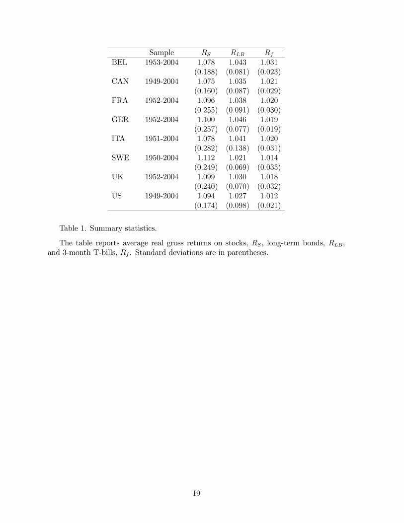
Sample RS RLB RfBEL 1953-2004 1:078 1:043 1:031
(0:188) (0:081) (0:023)CAN 1949-2004 1:075 1:035 1:021
(0:160) (0:087) (0:029)FRA 1952-2004 1:096 1:038 1:020
(0:255) (0:091) (0:030)GER 1952-2004 1:100 1:046 1:019
(0:257) (0:077) (0:019)ITA 1951-2004 1:078 1:041 1:020
(0:282) (0:138) (0:031)SWE 1950-2004 1:112 1:021 1:014
(0:249) (0:069) (0:035)UK 1952-2004 1:099 1:030 1:018
(0:240) (0:070) (0:032)US 1949-2004 1:094 1:027 1:012
(0:174) (0:098) (0:021)
Table 1. Summary statistics.
The table reports average real gross returns on stocks, RS, long-term bonds, RLB,and 3-month T-bills, Rf . Standard deviations are in parentheses.
19
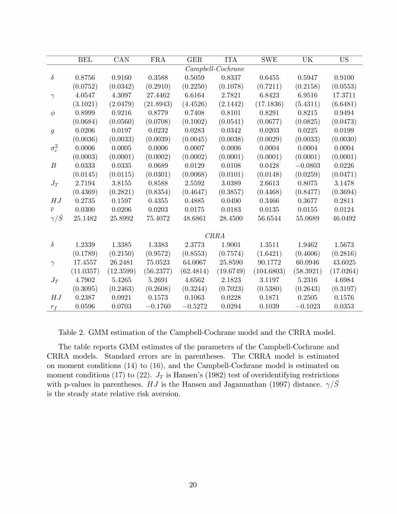
BEL CAN FRA GER ITA SWE UK USCampbell-Cochrane
� 0:8756 0:9160 0:3588 0:5059 0:8337 0:6455 0:5947 0:9100(0:0752) (0:0342) (0:2910) (0:2250) (0:1078) (0:7211) (0:2158) (0:0553)
4:0547 4:3097 27:4462 6:6164 2:7821 6:8423 6:9516 17:3711(3:1021) (2:0479) (21:8943) (4:4526) (2:1442) (17:1836) (5:4311) (6:6481)
� 0:8999 0:9216 0:8779 0:7408 0:8101 0:8291 0:8215 0:9494(0:0684) (0:0560) (0:0708) (0:1002) (0:0541) (0:0677) (0:0825) (0:0473)
g 0:0206 0:0197 0:0232 0:0283 0:0342 0:0203 0:0225 0:0199(0:0036) (0:0033) (0:0039) (0:0045) (0:0038) (0:0029) (0:0033) (0:0030)
�2c 0:0006 0:0005 0:0006 0:0007 0:0006 0:0004 0:0004 0:0004(0:0003) (0:0001) (0:0002) (0:0002) (0:0001) (0:0001) (0:0001) (0:0001)
B 0:0333 0:0335 0:0689 0:0129 0:0108 0:0428 �0:0803 0:0226(0:0145) (0:0115) (0:0301) (0:0068) (0:0101) (0:0148) (0:0259) (0:0471)
JT 2:7194 3:8155 0:8588 2:5592 3:0389 2:6613 0:8075 3:1478(0:4369) (0:2821) (0:8354) (0:4647) (0:3857) (0:4468) (0:8477) (0:3694)
HJ 0:2735 0:1597 0:4355 0:4885 0:0490 0:3466 0:3677 0:2811r 0:0300 0:0206 0:0203 0:0175 0:0183 0:0135 0:0155 0:0124 = �S 25:1482 25:8992 75:4072 48:6861 28:4500 56:6544 55:0689 46:0492
CRRA� 1:2339 1:3385 1:3383 2:3773 1:9001 1:3511 1:9462 1:5673
(0:1789) (0:2150) (0:9572) (0:8553) (0:7574) (1:6421) (0:4606) (0:2816) 17:4557 26:2481 75:0523 64:0067 25:8590 90:1772 60:0946 43:6025
(11:0357) (12:3599) (56:2377) (62:4814) (19:6749) (104:6803) (58:3921) (17:0264)JT 4:7902 5:4265 5:2691 4:6562 2:1823 3:1197 5:2316 4:6984
(0:3095) (0:2463) (0:2608) (0:3244) (0:7023) (0:5380) (0:2643) (0:3197)HJ 0:2387 0:0921 0:1573 0:1063 0:0228 0:1871 0:2505 0:1576rf 0:0596 0:0703 �0:1760 �0:5272 0:0294 0:1039 �0:1023 0:0353
Table 2. GMM estimation of the Campbell-Cochrane model and the CRRA model.
The table reports GMM estimates of the parameters of the Campbell-Cochrane andCRRA models. Standard errors are in parentheses. The CRRA model is estimatedon moment conditions (14) to (16), and the Campbell-Cochrane model is estimated onmoment conditions (17) to (22). JT is Hansen�s (1982) test of overidentifying restrictionswith p-values in parentheses. HJ is the Hansen and Jagannathan (1997) distance. = �Sis the steady state relative risk aversion.
20
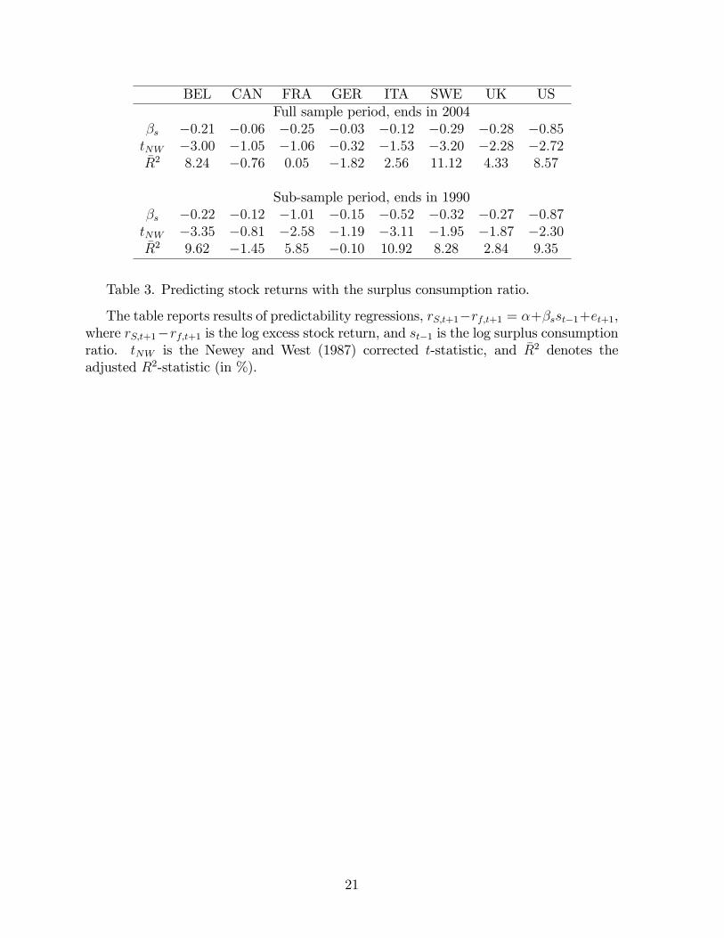
BEL CAN FRA GER ITA SWE UK USFull sample period, ends in 2004
�s �0:21 �0:06 �0:25 �0:03 �0:12 �0:29 �0:28 �0:85tNW �3:00 �1:05 �1:06 �0:32 �1:53 �3:20 �2:28 �2:72�R2 8:24 �0:76 0:05 �1:82 2:56 11:12 4:33 8:57
Sub-sample period, ends in 1990�s �0:22 �0:12 �1:01 �0:15 �0:52 �0:32 �0:27 �0:87tNW �3:35 �0:81 �2:58 �1:19 �3:11 �1:95 �1:87 �2:30�R2 9:62 �1:45 5:85 �0:10 10:92 8:28 2:84 9:35
Table 3. Predicting stock returns with the surplus consumption ratio.
The table reports results of predictability regressions, rS;t+1�rf;t+1 = �+�sst�1+et+1,where rS;t+1�rf;t+1 is the log excess stock return, and st�1 is the log surplus consumptionratio. tNW is the Newey and West (1987) corrected t-statistic, and �R2 denotes theadjusted R2-statistic (in %).
21
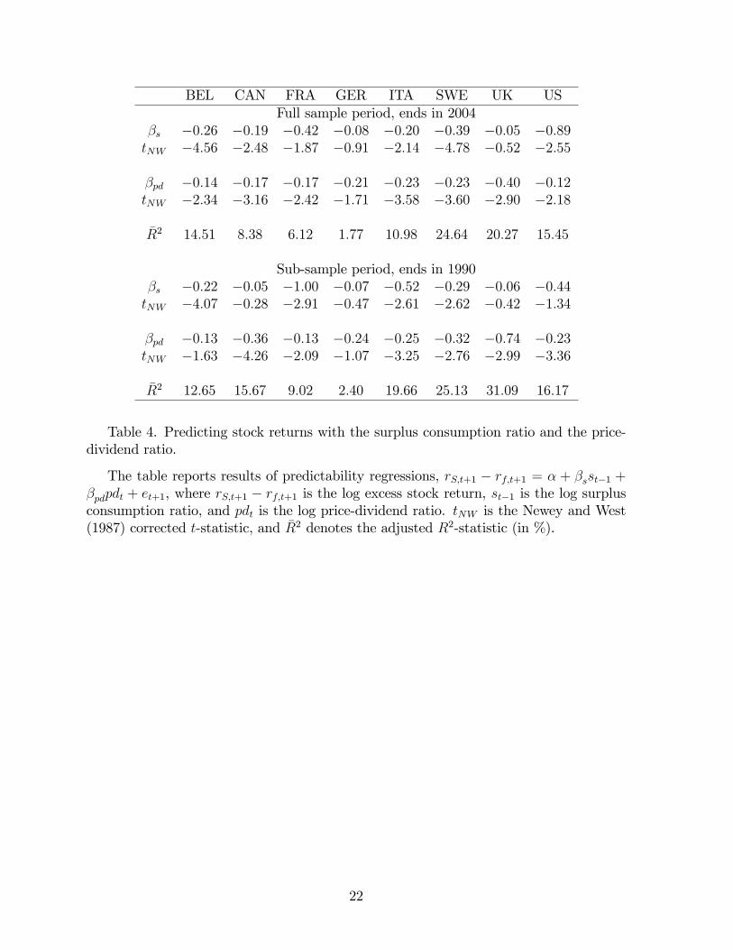
BEL CAN FRA GER ITA SWE UK USFull sample period, ends in 2004
�s �0:26 �0:19 �0:42 �0:08 �0:20 �0:39 �0:05 �0:89tNW �4:56 �2:48 �1:87 �0:91 �2:14 �4:78 �0:52 �2:55
�pd �0:14 �0:17 �0:17 �0:21 �0:23 �0:23 �0:40 �0:12tNW �2:34 �3:16 �2:42 �1:71 �3:58 �3:60 �2:90 �2:18
�R2 14:51 8:38 6:12 1:77 10:98 24:64 20:27 15:45
Sub-sample period, ends in 1990�s �0:22 �0:05 �1:00 �0:07 �0:52 �0:29 �0:06 �0:44tNW �4:07 �0:28 �2:91 �0:47 �2:61 �2:62 �0:42 �1:34
�pd �0:13 �0:36 �0:13 �0:24 �0:25 �0:32 �0:74 �0:23tNW �1:63 �4:26 �2:09 �1:07 �3:25 �2:76 �2:99 �3:36
�R2 12:65 15:67 9:02 2:40 19:66 25:13 31:09 16:17
Table 4. Predicting stock returns with the surplus consumption ratio and the price-dividend ratio.
The table reports results of predictability regressions, rS;t+1 � rf;t+1 = � + �sst�1 +�pdpdt + et+1, where rS;t+1 � rf;t+1 is the log excess stock return, st�1 is the log surplusconsumption ratio, and pdt is the log price-dividend ratio. tNW is the Newey and West(1987) corrected t-statistic, and �R2 denotes the adjusted R2-statistic (in %).
22
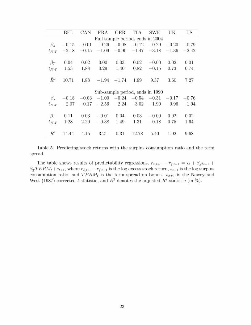
BEL CAN FRA GER ITA SWE UK USFull sample period, ends in 2004
�s �0:15 �0:01 �0:26 �0:08 �0:12 �0:29 �0:20 �0:79tNW �2:18 �0:15 �1:09 �0:90 �1:47 �3:18 �1:36 �2:42
�T 0:04 0:02 0:00 0:03 0:02 �0:00 0:02 0:01tNW 1:53 1:88 0:29 1:40 0:82 �0:15 0:73 0:74
�R2 10:71 1:88 �1:94 �1:74 1:99 9:37 3:60 7:27
Sub-sample period, ends in 1990�s �0:18 �0:03 �1:00 �0:24 �0:54 �0:31 �0:17 �0:76tNW �2:07 �0:17 �2:56 �2:24 �3:02 �1:90 �0:96 �1:94
�T 0:11 0:03 �0:01 0:04 0:03 �0:00 0:02 0:02tNW 1:28 2:20 �0:38 1:49 1:31 �0:18 0:75 1:64
�R2 14:44 4:15 3:21 0:31 12:78 5:40 1:92 9:68
Table 5. Predicting stock returns with the surplus consumption ratio and the termspread.
The table shows results of predictability regressions, rS;t+1 � rf;t+1 = � + �sst�1 +�TTERMt+et+1, where rS;t+1�rf;t+1 is the log excess stock return, st�1 is the log surplusconsumption ratio, and TERMt is the term spread on bonds. tNW is the Newey andWest (1987) corrected t-statistic, and �R2 denotes the adjusted R2-statistic (in %).
23
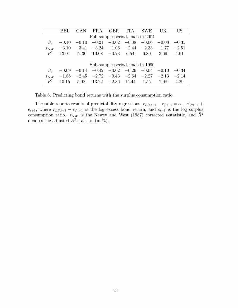
BEL CAN FRA GER ITA SWE UK USFull sample period, ends in 2004
�s �0:10 �0:10 �0:21 �0:02 �0:08 �0:06 �0:08 �0:35tNW �3:10 �3:41 �3:24 �1:06 �2:44 �2:33 �1:77 �2:51�R2 13:01 12:30 10:08 �0:73 6:54 6:80 3:69 4:61
Sub-sample period, ends in 1990�s �0:09 �0:14 �0:42 �0:02 �0:26 �0:04 �0:10 �0:34tNW �1:88 �2:45 �2:72 �0:43 �2:64 �2:27 �2:13 �2:14�R2 10:15 5:98 13:22 �2:36 15:44 1:55 7:08 4:29
Table 6. Predicting bond returns with the surplus consumption ratio.
The table reports results of predictability regressions, rLB;t+1 � rf;t+1 = �+ �sst�1 +et+1, where rLB;t+1 � rf;t+1 is the log excess bond return, and st�1 is the log surplusconsumption ratio. tNW is the Newey and West (1987) corrected t-statistic, and �R2
denotes the adjusted R2-statistic (in %).
24
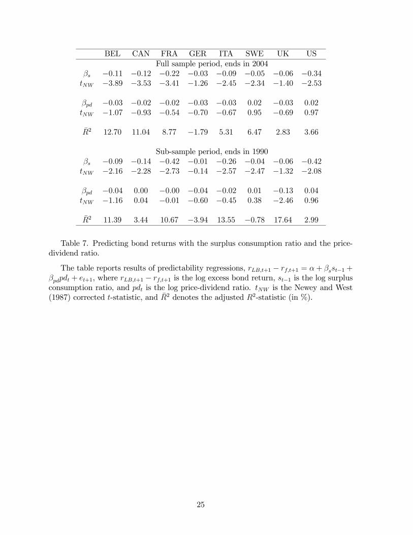
BEL CAN FRA GER ITA SWE UK USFull sample period, ends in 2004
�s �0:11 �0:12 �0:22 �0:03 �0:09 �0:05 �0:06 �0:34tNW �3:89 �3:53 �3:41 �1:26 �2:45 �2:34 �1:40 �2:53
�pd �0:03 �0:02 �0:02 �0:03 �0:03 0:02 �0:03 0:02tNW �1:07 �0:93 �0:54 �0:70 �0:67 0:95 �0:69 0:97
�R2 12:70 11:04 8:77 �1:79 5:31 6:47 2:83 3:66
Sub-sample period, ends in 1990�s �0:09 �0:14 �0:42 �0:01 �0:26 �0:04 �0:06 �0:42tNW �2:16 �2:28 �2:73 �0:14 �2:57 �2:47 �1:32 �2:08
�pd �0:04 0:00 �0:00 �0:04 �0:02 0:01 �0:13 0:04tNW �1:16 0:04 �0:01 �0:60 �0:45 0:38 �2:46 0:96
�R2 11:39 3:44 10:67 �3:94 13:55 �0:78 17:64 2:99
Table 7. Predicting bond returns with the surplus consumption ratio and the price-dividend ratio.
The table reports results of predictability regressions, rLB;t+1 � rf;t+1 = �+ �sst�1 +�pdpdt + et+1, where rLB;t+1 � rf;t+1 is the log excess bond return, st�1 is the log surplusconsumption ratio, and pdt is the log price-dividend ratio. tNW is the Newey and West(1987) corrected t-statistic, and �R2 denotes the adjusted R2-statistic (in %).
25
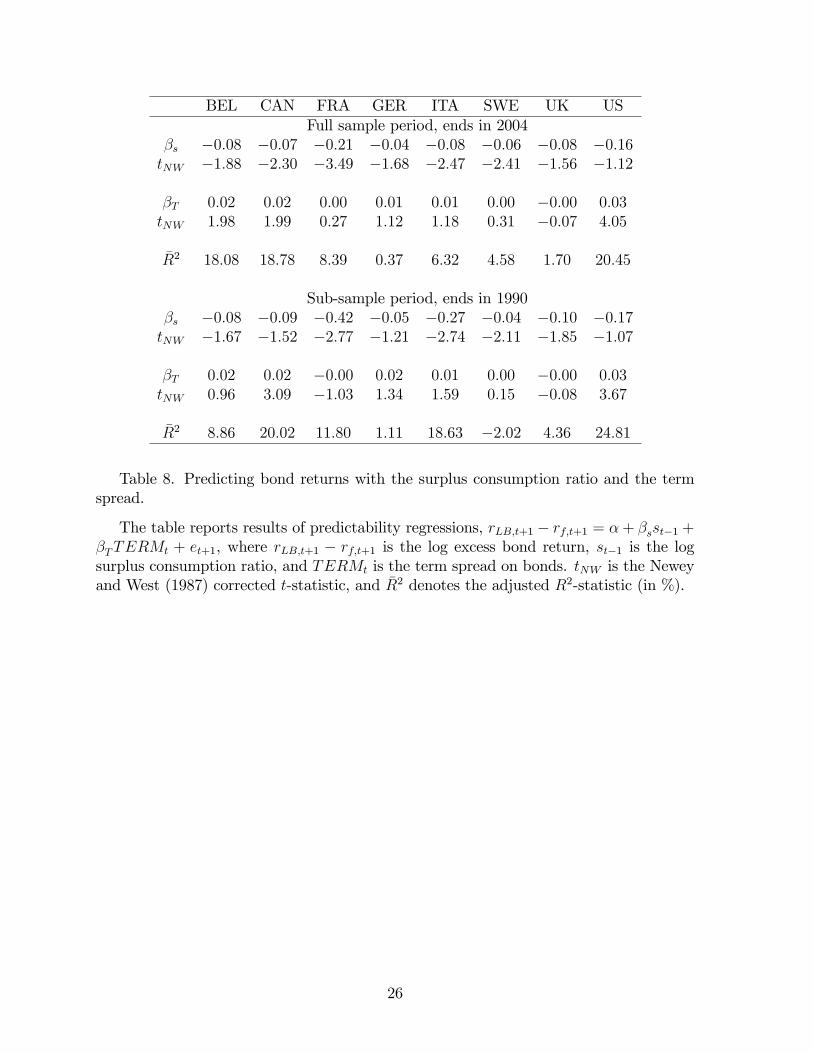
BEL CAN FRA GER ITA SWE UK USFull sample period, ends in 2004
�s �0:08 �0:07 �0:21 �0:04 �0:08 �0:06 �0:08 �0:16tNW �1:88 �2:30 �3:49 �1:68 �2:47 �2:41 �1:56 �1:12
�T 0:02 0:02 0:00 0:01 0:01 0:00 �0:00 0:03tNW 1:98 1:99 0:27 1:12 1:18 0:31 �0:07 4:05
�R2 18:08 18:78 8:39 0:37 6:32 4:58 1:70 20:45
Sub-sample period, ends in 1990�s �0:08 �0:09 �0:42 �0:05 �0:27 �0:04 �0:10 �0:17tNW �1:67 �1:52 �2:77 �1:21 �2:74 �2:11 �1:85 �1:07
�T 0:02 0:02 �0:00 0:02 0:01 0:00 �0:00 0:03tNW 0:96 3:09 �1:03 1:34 1:59 0:15 �0:08 3:67
�R2 8:86 20:02 11:80 1:11 18:63 �2:02 4:36 24:81
Table 8. Predicting bond returns with the surplus consumption ratio and the termspread.
The table reports results of predictability regressions, rLB;t+1 � rf;t+1 = �+ �sst�1 +�TTERMt + et+1, where rLB;t+1 � rf;t+1 is the log excess bond return, st�1 is the logsurplus consumption ratio, and TERMt is the term spread on bonds. tNW is the Neweyand West (1987) corrected t-statistic, and �R2 denotes the adjusted R2-statistic (in %).
26

BEL CAN FRA GER ITA SWE UK USFull sample period, ends in 2004
�AHs �0:19 �0:06 �0:17 �0:02 �0:09 �0:28 �0:29 �0:86tAH �2:10 �0:71 �0:63 �0:22 �1:16 �2:61 �1:84 �2:45
Sub-sample period, ends in 1990�AHs �0:19 �0:11 �0:97 �0:14 �0:51 �0:31 �0:28 �0:89tAH �1:79 �0:61 �1:70 �0:92 �2:28 �2:02 �1:47 �2:23
Table 9. Predicting stock returns with the surplus consumption ratio: Bias-adjustedresults.
The table reports the Amihud-Hurvich bias-adjusted beta estimates and t-statisticsusing the surplus consumption ratio to forecast the log excess stock return.
27

BEL CAN FRA GER ITA SWE UK USFull sample period, ends in 2004
�AHs �0:11 �0:12 �0:22 �0:03 �0:09 �0:06 �0:09 �0:36tAH �3:04 �3:21 �2:65 �0:91 �2:36 �2:15 �1:93 �1:93
Sub-sample period, ends in 1990�AHs �0:10 �0:15 �0:45 �0:02 �0:27 �0:04 �0:12 �0:33tAH �2:34 �2:00 �2:63 �0:43 �2:91 �1:10 �2:22 �1:60
Table 10. Predicting bond returns with the surplus consumption ratio: Bias-adjustedresults.
The table reports the Amihud-Hurvich bias-adjusted beta estimates and t-statisticsusing the surplus consumption ratio to forecast the log excess bond return.
28
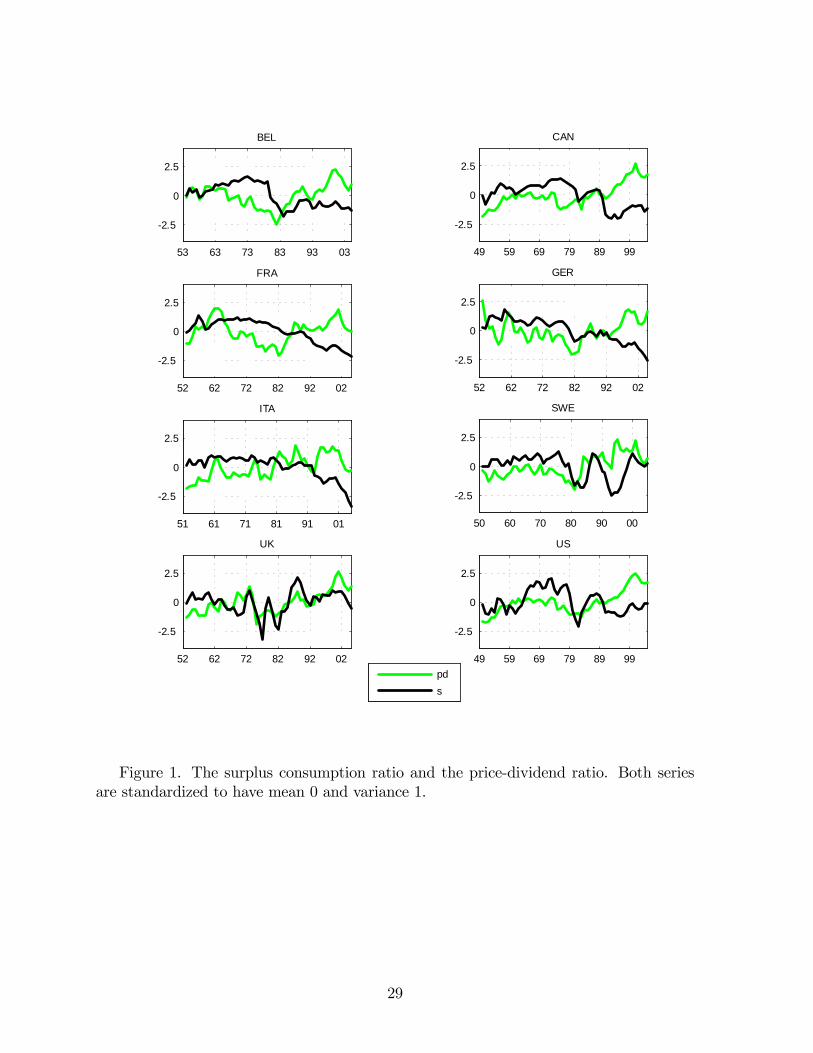
53 63 73 83 93 03
-2.5
0
2.5
BEL
49 59 69 79 89 99
-2.5
0
2.5
CAN
52 62 72 82 92 02
-2.5
0
2.5
FRA
52 62 72 82 92 02
-2.5
0
2.5
GER
51 61 71 81 91 01
-2.5
0
2.5
ITA
50 60 70 80 90 00
-2.5
0
2.5
SWE
49 59 69 79 89 99
-2.5
0
2.5
US
52 62 72 82 92 02
-2.5
0
2.5
UK
pds
Figure 1. The surplus consumption ratio and the price-dividend ratio. Both seriesare standardized to have mean 0 and variance 1.
29

Chapter 4
Consumption growth and time-varying expected stock returns
Consumption growth and time-varying expectedstock returns�
Stig Vinther Møllery
Published in
Finance Research Letters, 2008 volume 5, pages 129-136.
Abstract
When the consumption growth rate is measured based upon fourth quarterdata, it tracks predictable variation in future excess stock returns. Low fourthquarter consumption growth rates predict high future excess stock returns suchthat expected returns are high at business cycle troughs and low at business cyclepeaks. The consumption growth rate loses predictive power when it is measuredbased upon other quarters. This is consistent with the insight of Jagannathanand Wang (2007) that investors tend to review their consumption and investmentplans during the end of each calendar year, and at possibly random times in be-tween. The consumption growth rate measured based upon fourth quarter data isa much stronger predictive variable than benchmark predictive variables such asthe dividend-price ratio, the term spread, and the default spread.
Keywords: Return predictability; Consumption growthJEL codes: C12; E21; E44; G12
�I thank Tom Engsted, Richard Priestley and an anonymous referee for helpful comments.yAarhus School of Business, University of Aarhus, Fuglesangs Allé 4, DK-8210 Aarhus V., Denmark,
and CREATES (Center for Research in Econometric Analysis of Time Series), funded by the DanishNational Research Foundation. E-mail: [email protected].
1
1 Introduction
An extensive empirical literature in �nance has demonstrated that expected stock returnsvary over time. Campbell and Shiller (1988) and Fama and French (1988, 1989) amongothers use �nancial predictive variables based on stock and bond market data such asthe dividend-price ratio, the term spread, and the default spread to document that stockreturns display predictable variation over time. Fama and French (1989) link the �nancialpredictive variables to the business cycle and suggest that investors require a higherexpected return at a business cycle trough than they do at a business cycle peak. Morerecently, macro predictive variables such as the consumption-wealth ratio (Lettau andLudvigson 2001) have been shown to predict stock returns providing a direct linkagebetween time-varying expected returns and the business cycle.1
This paper examines the ability of the consumption growth rate to capture predictablevariation in stock returns over the business cycle. The consumption growth rate has aclear business cycle pattern and is closely related to the business cycles as measured by theNational Bureau of Economic Research (NBER). To mitigate the e¤ect of measurementerror in consumption data as well as the e¤ect of infrequent adjustment of consumptionplans that may disrupt the linkage between the consumption growth rate and expectedreturns, I follow Jagannathan and Wang (2007) and measure the consumption growthrate based upon fourth quarter data. I examine the predictive power of the fourthquarter consumption growth rate by running regressions of future excess stock returnson the lagged fourth quarter consumption growth rate. I �nd strong support for theability of the fourth quarter consumption growth rate to predict future excess stockreturns using US post-war data from 1947 to 2005. The �R2-statistic is as high as 19%at the 1-year horizon, and the slope estimate is strongly signi�cantly negative such thatlow consumption growth rates predict high future excess stock returns. Hence, expectedreturns are high at business cycle troughs and low at business cycle peaks, which isconsistent with the �ndings of Fama and French (1989). The fourth quarter consumptiongrowth rate � a pure macroeconomic variable � is a much stronger predictive variablethan the traditional �nancial predictive variables such as the dividend-price ratio, theterm spread, and the default spread. In fact, the fourth quarter consumption growth ratedrives out the �nancial predictive variables in multiple regressions. Moreover, the fourthquarter consumption growth rate also provides substantial additional information aboutfuture excess stock returns beyond that contained in the consumption-wealth ratio.
The consumption growth rate loses predictive power when it is measured based uponother quarters. This is consistent with the insight of Jagannathan and Wang (2007) thatinvestors tend to review their consumption and investment plans during the end of eachcalendar year, and at possibly random times in between. Possible explanations includemore leisure time during the Christmas holiday season, the resolution of uncertaintyabout end of year bonuses, and end of year tax consequences of portfolio choices; seeJagannathan and Wang (2007) and the references therein.
1See Cochrane (2007) for a comprehensive survey on the return predictability literature.
2
The fourth quarter consumption growth rate has a number of distinct properties asa predictive variable. First of all, the fourth quarter consumption growth rate is a puremacroeconomic variable that provides a direct linkage between time-varying expectedreturns and the business cycle. In addition, the fourth quarter consumption growth rateis easily constructed from the National Income and Product Accounts (NIPA) and doesnot rely on estimating a cointegration relationship (such as for example the consumption-wealth ratio). Finally, the fourth quarter consumption growth rate is an almost i.i.d.process and is much less persistent than alternative predictive variables. Given the con-troversy about return predictability using highly persistent predictive variables, it isnoteworthy that the fourth quarter consumption growth rate � an almost i.i.d. process� can predict future stock returns.2
2 Data
The empirical analysis is based on US post-war data for the period 1947 to 2005. Con-sumption is measured as seasonally adjusted real per capita expenditures on non-durablesand services. The consumption data is obtained from the National Income and ProductAccounts (NIPA) and is available on quarterly frequency starting from 1947. The an-nual log excess stock return is calculated as the log return on the value weighted CRSPindex including NYSE, AMEX, and NASDAQ �rms minus the log return on a 3-monthTreasury bill rate. As benchmark predictive variables, I use the log dividend-price ratio(dpt), the term spread between long-term government bond yields and Treasury bill yields(TERMt), the default spread between BAA and AAA corporate bond yields (DEFt),and the consumption-wealth ratio (dcayt). dpt is derived from CRSP value weighted re-turns with and without dividend capitalization. TERMt, DEFt, anddcayt are obtainedfrom Amit Goyal�s website.
Table 1 provides summary statistics of the consumption growth rate. In the upperpanel, the consumption growth rate is measured annually as year to year growth ratesin quarterly consumption, i.e. 4Q-4Q is the consumption growth rate calculated fromthe fourth quarter in year t � 1 to the fourth quarter in year t. In the lower panel,the consumption growth rate is measured quarterly, i.e. 3Q-4Q is the fourth quarterconsumption growth rate calculated from the third quarter in year t to the fourth quarterin year t. The means and standard deviations of the year to year growth rates in quarterlyconsumption are similar across quarters, but the range is largest for the fourth quarter.This replicates the �ndings of Jagannathan and Wang (2007). Moreover, the quarterlyconsumption growth rate has a higher standard deviation and range in the fourth quartercompared to the �rst, second and third quarters.
Figure 1 plots the annual 4Q-4Q consumption growth rate and the quarterly 3Q-4Qconsumption growth rate. The shaded areas represent the NBER recession dates. Theannual 4Q-4Q consumption growth rate and the quarterly 3Q-4Q consumption growth
2Stambaugh (1999) demonstrates that the use of highly persistent predictive variables may lead tospurious evidence of return predictability.
3
rate have similar patterns, but the latter is more volatile and takes on more extreme valuesat peaks and troughs than the former. The correlation coe¢ cient between the two seriesis 0:63. Furthermore, the �gure illustrates two distinct properties of the consumptiongrowth rate as a predictive variable. First, the consumption growth rate has a clearbusiness cycle pattern; it rises during business cycle expansions and reaches its highestvalues near peaks and falls during business contractions and reaches its lowest valuesnear troughs. For instance, the consumption growth rate drops substantially just afterthe recession years of the oil shock of 1973-1975. Second, the consumption growth ratehas a very low degree of persistence, implying that the consumption growth rate doesnot su¤er from the statistical problems that arise using a highly persistent predictivevariable, cf. Stambaugh (1999).
3 Predicting stock returns
Now I turn to testing the ability of consumption growth rates to predict future excessstock returns. This is done by 1-year ahead predictive regressions:
ret+1 = �+ �Gct + et+1; (1)
where ret+1 is the 1-year ahead log excess stock return and Gct is the consumption growth
rate. Table 2 reports OLS estimates, Newey and West (1987) corrected t-statistics, and�R2-statistics. Signi�cant estimates at the �ve percent level are in bold. The upper panelof Table 2 reports the results for annual consumption growth rates measured as yearto year growth rates in quarterly consumption. When the annual consumption growthrate is based upon fourth quarter data, it tracks a substantial amount of the variationin future excess stock returns. The �R2-statistic is 12:01%, and the slope estimate issigni�cantly negative such that low consumption growth rates predict high future excessstock returns, i.e. expected returns are high at business cycle troughs and low at businesscycle peaks. When the annual consumption growth rate is measured based upon otherquarters, it loses predictive power; both the t-statistic and the �R2-statistic fall. The lowerpanel of Table 2 reports the results for quarterly consumption growth rates. Here theevidence is even more striking. The fourth quarter consumption growth rate produces an�R2-statistic of 18:89%, and the slope estimate is strongly signi�cant (t-statistic of �5:75).When the quarterly consumption growth rate is measured based upon the �rst, second,and third quarters, the slope estimates are borderline signi�cant or insigni�cant, and the�R2-statistics are negligible. These dramatic results relate to the �ndings of JagannathanandWang (2007). They emphasize that the use of fourth quarter data mitigates the e¤ectof measurement error in consumption data as well as the e¤ect of infrequent adjustmentof consumption plans that may disrupt the linkage between the consumption growth rateand expected returns.
The above evidence implies that both the 4Q-4Q and 3Q-4Q consumption growthrates have predictive power for future excess stock returns. The 4Q-4Q (annual) con-sumption growth rate is the sum of the 4Q-3Q (�rst three quarters) and the 3Q-4Q
4
(fourth quarter) consumption growth rates. To examine whether the 4Q-3Q consump-tion growth rate also predicts future excess stock returns, I regress the 1-year aheadcalendar year excess stock return on the 4Q-3Q consumption growth rate. The slopeestimate is �3:24, the Newey-West corrected t-statistic is �1:66, and the �R2-statistic is3:31. Hence, the consumption growth rate of the �rst three quarters does not containmuch predictive power for future excess stock returns, implying that the predictive powerof the consumption growth rate is related to the fourth quarter.
3.1 Controlling for benchmark predictive variables
To control for benchmark predictive variables, I run predictive regressions of the form:
ret+1 = �+ �Gct + �
0Zt + et+1; (2)
where Zt is a vector of benchmark predictive variables and Gct is the fourth quarterconsumption growth rate. I compare the performance of Gct with traditional �nancialpredictive variables (dpt, TERMt, and DEFt) and the most prominent macro predictivevariable (dcayt). The benchmark predictive variables are measured on an annual frequency.Table 3 shows that Gct contains substantial additional information about future excessstock returns relative to the traditional �nancial predictive variables. dpt has a signi�cantslope estimate and explains 6:86% of the variation in 1-year ahead excess stock returns,whereas TERMt and DEFt are not able to predict excess stock returns in the post-warperiod from 1947 to 2005; their slope estimates are insigni�cant, and the �R2-statistics areclose to zero or negative. When Gct is included in the predictive regression with dpt, the�R2-statistic increases to 22:34%, and the slope estimate turns out to be insigni�cant fordpt. Table 3 shows that Gct is also robust to the inclusion ofdcayt. dcayt has a signi�cantslope estimate, and it produces an �R2-statistic of 17:48% as a sole predictive variable.By including Gct along withdcayt, the �R2-statistic increases to 29:57% and both predictivevariables remain signi�cant. To con�rm the robustness, I run a predictive regression thatincludes all the predictive variables; Gct , dpt, TERMt, DEFt and dcayt. The �nancialpredictive variables (dpt, TERMt and DEFt) are all insigni�cant, and the �R2-statisticdoes not increase once these variables are included. Hence, the relevant informationabout future excess stock returns is contained in Gct anddcayt; macro predictive variablesthat provide a direct linkage between time-varying expected returns and the businesscycle.
As a further robustness check, I examine the predictive power of the benchmarkpredictive variables measured based upon fourth quarter data. Table 4 shows that thepredictive power of dpt anddcayt does not change much when they are measured basedupon fourth quarter data instead of annual data.3 dpt produces an �R2-statistic of 7:89%on fourth quarter data compared to 6:86% on annual data, whereasdcayt produces an �R2-statistic of 13:75% on fourth quarter data compared to 17:48% on annual data.4 Both
3I only report results for dpt anddcayt since both TERMt and DEFt produce the same results withfourth quarter data as they do with annual data.
4Fordcayt the fourth quarter data starts in 1951, while the annual data starts in 1948.5
dpt anddcayt continue to be signi�cant as sole predictive variables, but turn insigni�cantwhen Gct is included to the predictive regression. Overall, the evidence suggests that thefourth quarter e¤ect is a pure consumption e¤ect.
3.2 Small sample bias
This section deals with small sample bias in the predictive regression (1). Specifyingthe predictive variable (xt) as a stationary �rst-order autoregressive process, Stambaugh(1999) sets up the following model:
ret+1 = �+ �xt + et+1; et+1 � niid�0; �2e
�(3)
xt+1 = � + �xt + ut+1; ut+1 � niid�0; �2u
�(4)
and derives the small sample bias in � as a function of the degree of persistence in xt andthe correlation between the innovations in (3) and (4). Stambaugh (1999) shows thatthe small sample bias is particularly severe for �nancial predictive variables such as thedividend-price ratio since it is highly persistent, and its innovations are highly correlatedwith the innovations in returns. The small sample bias is less relevant with the fourthquarter consumption growth rate as predictive variable for two reasons. First, the fourthquarter consumption growth rate is not highly persistent. It has an AR(1) coe¢ cient of�0:05, whereas the dividend-price ratio has an AR(1) coe¢ cient of 0:95. Second, since thefourth quarter consumption growth rate is a pure macroeconomic variable, its innovationshave relatively low correlation with the innovations in returns. The correlation betweenthe innovations in the fourth quarter consumption growth rate and the innovations inthe excess stock return is 0:27, whereas the correlation between the innovations in thedividend-price ratio and the innovations in the excess stock return is �0:61. To con�rmthat small sample bias is not an issue, I apply the following bootstrap procedure:
First, I estimate the following model, where Gct is the fourth quarter consumptiongrowth rate:
ret+1 = �+ et+1; (5)
Gct+1 = � + �Gct + ut+1: (6)
Following the common practice (Nelson and Kim 1993, Goetzmann and Jorion 1993, andKothari and Shanken 1997), I bootstrap under the null of no predictability by imposingthe constraint that � = 0 and assume that the predictive variable follows an AR(1)model.5 Second, I construct 100; 000 bootstrap samples of length T +1; 000 by randomlyselecting residual pairs from (5) and (6). I use the OLS estimates of �, �, and �, and setthe initial values of ret and G
ct equal to their sample averages. The �rst 1; 000 observations
are thrown away to avoid any e¤ects from using the sample averages as starting values.Third, I estimate � from each bootstrap sample using equation (1) and then calculate a
5I have also used an AR(2) model as the data generating process for Gct . The AR(2) coe¢ cient is�0:32. Using an AR(2) model produces nearly identical results as the AR(1) model.
6
95% bootstrap con�dence interval for � using the lower 2.5th percentile and the upper97.5th percentile of the 100; 000 bootstrap samples.
The average value of the 100; 000 arti�cial slope coe¢ cients simulated under the nullof no predictability is �0:03, and the 95% bootstrap con�dence interval is [�1:94; 1:90].Since the con�dence interval does not include the OLS estimate �̂ = �3:19 (reportedin Table 2), the bootstrap analysis con�rms the conclusion that the fourth quarter con-sumption growth ratio predicts future excess stock returns.
4 Conclusion
This paper shows that the consumption growth rate based upon fourth quarter datatracks predictable variation in future excess stock returns. When the consumption growthrate is measured based upon other quarters, it loses predictive power. This is consistentwith Jagannathan and Wang (2007) who emphasize that the use of fourth quarter datamitigates the e¤ect of measurement error in consumption data as well as the e¤ect ofinfrequent adjustment of consumption plans that may disrupt the linkage between theconsumption growth rate and expected returns.
The fourth quarter consumption growth rate is a pure macroeconomic variable andprovides a direct linkage between time-varying expected returns and the business cycles; itpredicts high excess stock returns at business cycle troughs and low excess stock returns atbusiness cycle peaks. The fourth quarter consumption growth rate outperforms �nancialpredictive variables such as the dividend-price ratio, the term spread, and the defaultspread. The fourth quarter consumption growth rate also provides statistically signi�cantadditional information about future excess stock returns beyond that contained in theconsumption-wealth ratio. Importantly, the fourth quarter consumption growth rate is analmost i.i.d. process, which eliminates potential concerns about �nding spurious evidenceof return predictability, cf. Stambaugh (1999).
7

References
[1] Campbell, J.Y., Shiller, R., 1988. The dividend-price ratio and expectations of futuredividends and discount factors. Review of Financial Studies 1, 195-208.
[2] Cochrane, J.H., 2007. Financial markets and the real economy. In: Mehra, R., Theequity premium, North Holland Handbook of Finance Series, North Holland, Ams-terdam.
[3] Fama, E.F., French, K.R., 1988. Dividend yields and expected stock returns. Journalof Financial Economics 22, 3-25.
[4] Fama, E.F., French, K.R., 1989. Business conditions and expected returns on stocksand bonds. Journal of Financial Economics 25, 23-49.
[5] Goetzmann, W., Jorian, P., 1993. Testing the predictive value of dividend yields.Journal of Finance 48, 1087-1088.
[6] Jagannathan, R., Wang, Y., 2007. Lazy investors, discretionary consumption, andthe cross-section of stock returns, Journal of Finance 62, 1623-1661.
[7] Kothari, S.P., Shanken, J., 1997. Book-to-market, dividend yield, and expectedmarket returns: A time-series analysis. Journal of Financial Economics 44, 169-203.
[8] Lettau, M., Ludvigson, S., 2001. Consumption, aggregate wealth and expected re-turns. Journal of Finance 55, 815-849.
[9] Nelson, C.R., Kim, M.J., 1993. Predictable stock returns: The role of small samplebias. Journal of Finance 48, 641-661.
[10] Newey, W.K., West, K.D., 1987. A simple, positive semide�nite, heteroskedasticityand autocorrelation consistent covariance matrix. Econometrica 55, 703-708.
[11] Stambaugh, R.F., 1999. Predictive regressions. Journal of Financial Economics 54,375-421.
8
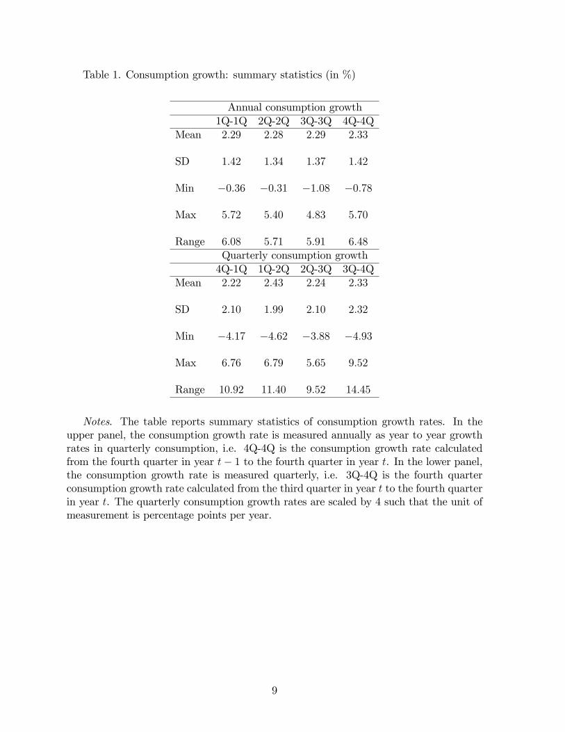
Table 1. Consumption growth: summary statistics (in %)
Annual consumption growth1Q-1Q 2Q-2Q 3Q-3Q 4Q-4Q
Mean 2:29 2:28 2:29 2:33
SD 1:42 1:34 1:37 1:42
Min �0:36 �0:31 �1:08 �0:78
Max 5:72 5:40 4:83 5:70
Range 6:08 5:71 5:91 6:48Quarterly consumption growth4Q-1Q 1Q-2Q 2Q-3Q 3Q-4Q
Mean 2:22 2:43 2:24 2:33
SD 2:10 1:99 2:10 2:32
Min �4:17 �4:62 �3:88 �4:93
Max 6:76 6:79 5:65 9:52
Range 10:92 11:40 9:52 14:45
Notes. The table reports summary statistics of consumption growth rates. In theupper panel, the consumption growth rate is measured annually as year to year growthrates in quarterly consumption, i.e. 4Q-4Q is the consumption growth rate calculatedfrom the fourth quarter in year t� 1 to the fourth quarter in year t. In the lower panel,the consumption growth rate is measured quarterly, i.e. 3Q-4Q is the fourth quarterconsumption growth rate calculated from the third quarter in year t to the fourth quarterin year t. The quarterly consumption growth rates are scaled by 4 such that the unit ofmeasurement is percentage points per year.
9
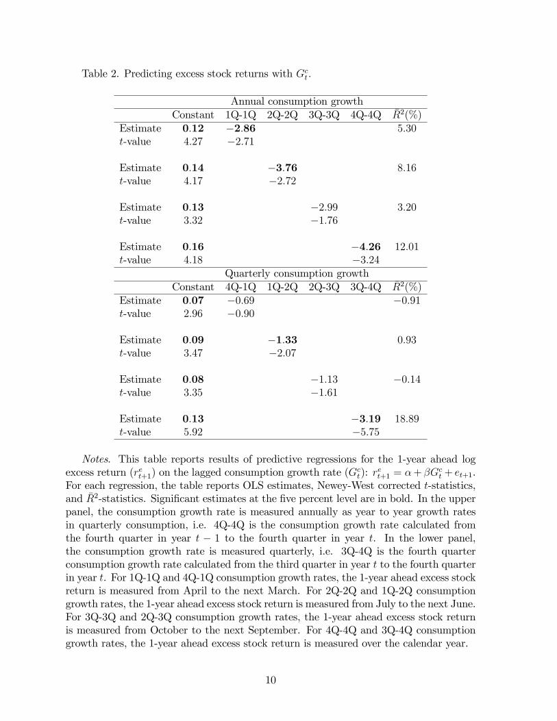
Table 2. Predicting excess stock returns with Gct :
Annual consumption growthConstant 1Q-1Q 2Q-2Q 3Q-3Q 4Q-4Q �R2(%)
Estimate 0:12 �2:86 5:30t-value 4:27 �2:71
Estimate 0:14 �3:76 8:16t-value 4:17 �2:72
Estimate 0:13 �2:99 3:20t-value 3:32 �1:76
Estimate 0:16 �4:26 12:01t-value 4:18 �3:24
Quarterly consumption growthConstant 4Q-1Q 1Q-2Q 2Q-3Q 3Q-4Q �R2(%)
Estimate 0:07 �0:69 �0:91t-value 2:96 �0:90
Estimate 0:09 �1:33 0:93t-value 3:47 �2:07
Estimate 0:08 �1:13 �0:14t-value 3:35 �1:61
Estimate 0:13 �3:19 18:89t-value 5:92 �5:75
Notes. This table reports results of predictive regressions for the 1-year ahead logexcess return (ret+1) on the lagged consumption growth rate (G
ct): r
et+1 = �+ �G
ct + et+1.
For each regression, the table reports OLS estimates, Newey-West corrected t-statistics,and �R2-statistics. Signi�cant estimates at the �ve percent level are in bold. In the upperpanel, the consumption growth rate is measured annually as year to year growth ratesin quarterly consumption, i.e. 4Q-4Q is the consumption growth rate calculated fromthe fourth quarter in year t � 1 to the fourth quarter in year t. In the lower panel,the consumption growth rate is measured quarterly, i.e. 3Q-4Q is the fourth quarterconsumption growth rate calculated from the third quarter in year t to the fourth quarterin year t. For 1Q-1Q and 4Q-1Q consumption growth rates, the 1-year ahead excess stockreturn is measured from April to the next March. For 2Q-2Q and 1Q-2Q consumptiongrowth rates, the 1-year ahead excess stock return is measured from July to the next June.For 3Q-3Q and 2Q-3Q consumption growth rates, the 1-year ahead excess stock returnis measured from October to the next September. For 4Q-4Q and 3Q-4Q consumptiongrowth rates, the 1-year ahead excess stock return is measured over the calendar year.
10
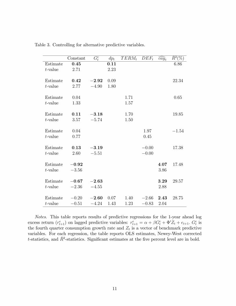
Table 3. Controlling for alternative predictive variables.
Constant Gct dpt TERMt DEFt dcayt �R2(%)Estimate 0:45 0:11 6:86t-value 2:71 2:23
Estimate 0:42 �2:92 0:09 22:34t-value 2:77 �4:90 1:80
Estimate 0:04 1:71 0:65t-value 1:33 1:57
Estimate 0:11 �3:18 1:70 19:85t-value 3:57 �5:74 1:50
Estimate 0:04 1:97 �1:54t-value 0:77 0:45
Estimate 0:13 �3:19 �0:00 17:38t-value 2:60 �5:51 �0:00
Estimate �0:92 4:07 17:48t-value �3:56 3:86
Estimate �0:67 �2:63 3:29 29:57t-value �2:36 �4:55 2:88
Estimate �0:20 �2:60 0:07 1:40 �2:66 2:43 28:75t-value �0:51 �4:24 1:43 1:23 �0:83 2:04
Notes. This table reports results of predictive regressions for the 1-year ahead logexcess return (ret+1) on lagged predictive variables: r
et+1 = � + �G
ct + �
0Zt + et+1: Gct is
the fourth quarter consumption growth rate and Zt is a vector of benchmark predictivevariables. For each regression, the table reports OLS estimates, Newey-West correctedt-statistics, and �R2-statistics. Signi�cant estimates at the �ve percent level are in bold.
11
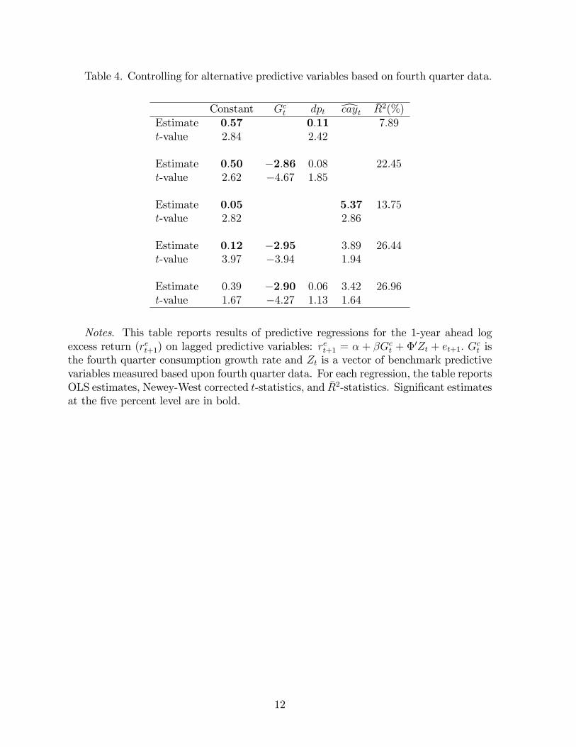
Table 4. Controlling for alternative predictive variables based on fourth quarter data.
Constant Gct dpt dcayt �R2(%)Estimate 0:57 0:11 7:89t-value 2:84 2:42
Estimate 0:50 �2:86 0:08 22:45t-value 2:62 �4:67 1:85
Estimate 0:05 5:37 13:75t-value 2:82 2:86
Estimate 0:12 �2:95 3:89 26:44t-value 3:97 �3:94 1:94
Estimate 0:39 �2:90 0:06 3:42 26:96t-value 1:67 �4:27 1:13 1:64
Notes. This table reports results of predictive regressions for the 1-year ahead logexcess return (ret+1) on lagged predictive variables: r
et+1 = � + �G
ct + �
0Zt + et+1: Gct is
the fourth quarter consumption growth rate and Zt is a vector of benchmark predictivevariables measured based upon fourth quarter data. For each regression, the table reportsOLS estimates, Newey-West corrected t-statistics, and �R2-statistics. Signi�cant estimatesat the �ve percent level are in bold.
12
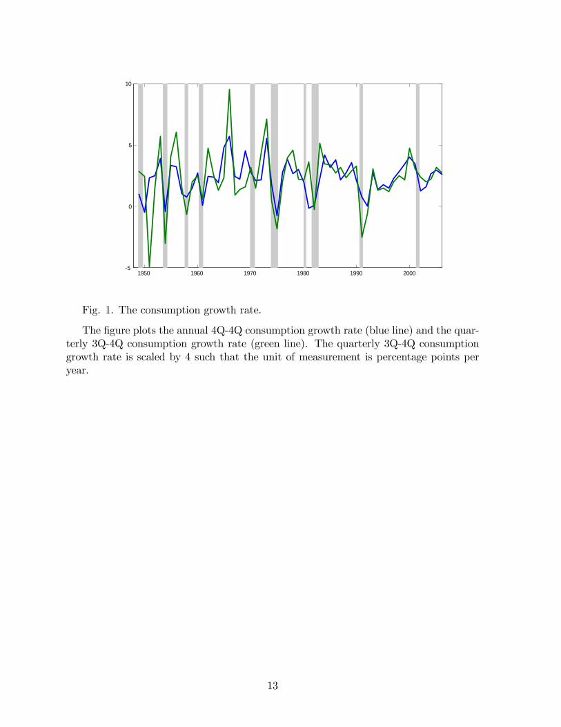
1950 1960 1970 1980 1990 2000-5
0
5
10
Fig. 1. The consumption growth rate.
The �gure plots the annual 4Q-4Q consumption growth rate (blue line) and the quar-terly 3Q-4Q consumption growth rate (green line). The quarterly 3Q-4Q consumptiongrowth rate is scaled by 4 such that the unit of measurement is percentage points peryear.
13
Recommended


![CaseReport Habit Breaking Appliance for Multiple Corrections · Habit Breaking Appliance for Multiple Corrections ... removable habit breaking appliances [15, 16]. Hence, habit breaking](https://img.dokumen.tips/doc/110x75/5f15893424a8522d646af1b7/casereport-habit-breaking-appliance-for-multiple-corrections-habit-breaking-appliance.jpg)