Geometry, Kinematics, and Rigid BodyMechanics in Cayley-Klein Geometries

Charles G. Gunn

Abstract. The 19th century witnessed a dramatic freeing of the human in-tellect from its naive assumptions. This development is particularly striking inmathematics. New geometries were discovered which challenged and expandedthe familiar space of euclid, notably projective geometry and non-euclideanmetric geometries. Developments in algebra led to similarly earth-shaking dis-coveries. This expansion of consciousness was accompanied by a desire to find ahigher unity in the growing diversity. Hermann Grassmann made a bold, earlyattempt to bring the two domains together in his ”Science of extension” of1844. Later in the century, Cayley and Klein contributed to this process bytheir discovery that metric geometry could be constructed atop projective ge-ometry. William Clifford introduced a geometric product combining the metricinner product with Grassmann’s exterior product; the resulting structure hasbecome known as a Clifford or geometric algebra. A completely satisfactory for-mulation of geometric algebra had to await the rigorous clarity of 20th centurymathematics.

The work presented here (the author’s Ph. D. thesis from the TechnicalUniversity Berlin, 2011) represents an attempt to bring this stream of 19th

century mathematics into the aforementioned rigorous, modern form, and toapply the resulting thought forms to understand kinematics and rigid bodymechanics in the spaces under consideration (including euclidean, hyperbolicand elliptic space). One guiding light in the treatment is the reliance on a pro-jective geometric foundation throughout, particularly a consequent applicationof the principle of duality. This projective approach guarantees that the resultis metric-neutral – the results are stated in such a way that they apply equallywell to the two non-euclidean geometries as well as euclidean geometry. And aconsequent consideration of duality leads to the recognition that this classicaltriad must be extended by a fourth geometry, dual euclidean geometry.

Readers of the MPK will not be surprised to learn that dual euclidean geom-etry has a close affinity with counter-space [in German, Gegenraum], a conceptwhich Rudolf Steiner introduced and developed, particularly in his natural sci-ence lectures. That such a connection exists in the work presented here is notsurprising, as the initial impulse for this thesis was provided by the later worksof George Adams (for example, see [Ada59]), to whom the present publicationis dedicated. One of Adams’ great gifts was to show how the results of modernscience, particularly mathematical, when grasped with enlivened thinking, re-veal deep, often unexpected, connections to the world and the human being –in a manner reminiscent of Goethe’s reading the “open secrets” of nature. Suchinsights can indicate fruitful directions for further research. In this spirit is thecurrent publication offered, with special thanks to Peter Gschwind for makingit possible.

3

Preface

This thesis arose out of a desire to understand and simulate rigid body motionin 2- and 3-dimensional spaces of constant curvature.The results are arrangedin a theoretical part and a practical part. The theoretical part first constructsnecessary tools – a family of real projective Clifford algebras – which representthe geometric relations within the above-mentioned spaces with remarkablefidelity. These tools are then applied to represent kinematics and rigid bodydynamics in these spaces, yielding a complete description of rigid body motionthere. The practical part describes simulation and visualization results basedon this theory.

Historically, the contents of this work flow out of the stream of 19th centurymathematics due to Chasles, Mobius, Plucker, Klein, and others, which success-fully applied new methods, mostly from projective geometry, to the problem ofrigid body motion. The excellent historical monograph [Zie85] coined the namegeometric mechanics expressly for this domain1. Its central concepts belongto the geometry of lines in three-dimensional projective space. The theoret-ical part of the thesis is devoted to formulating and occasionally extendingthese concepts in a modern, metric-neutral way using the real Clifford algebrasmentioned above.

Autobiographically, the current work builds on previous work ([Gun93])which explored visualization of three-dimensional manifolds modeled on one ofthese three constant curvature spaces. The dream of extending this geometric-visualization framework to include physics in these spaces – analogous to howin the past two decades the mainstream euclidean visualization environmentshave been gradually extended to include physically-based modeling – was apersonal motivation for undertaking the research which led to this thesis.

1 although today there are other meanings for this term.

4

Audience

The thesis is written with a variety of audiences in mind. In the foregroundis the desire to present a rigourous, self-contained, metric-neutral elaborationof the mathematical results, both old and new. It is however not written forthe specialist alone. For those interested only in the euclidean theory I haveattempted to make it accessible to readers without background or interest inthe non-euclidean thread. To be self-contained, many preliminary results fromprojective geometry and linear and multi-linear algebra are stated, with refer-ences to proofs in the literature. To be accessible, most of the results are statedand proved only for the dimensions n = 2 and n = 3, even when a general proofmight present no extra difficulty. The exposition includes many examples, par-ticularly euclidean ones, in which the reader can familiarize himself with thecontent. I have attempted at the ends of chapters to provide a guide to originalliterature for those interested in exploring further. Finally, as a firm believer inthe value of pictures, I have tried to illustrate the text wherever possible.

Outline

Chapter 1 introduces the important themes of the thesis via the well-knownexample of the Euler top, and shows how by generalizing the Euler top one isled to the topic of the thesis. In addition to reviewing the key ingredients ofrigid body motion, it contrasts the historical approaches of Euler and Poinsotto the problem, and relates these to the approach taken here. It discussesthe appropriate algebraic representation for the mathematical problems beingconsidered. It shows how quaternions can be used to represent the Euler top,and specifies a set of properties which an algebraic structure should possess inorder to serve the same purpose for the extended challenge posed by the thesis.

Chapter 2 introduces the non-metric foundations of the thesis. The geometricfoundation is provided by real projective geometry. From this is constructedthe Grassmann, or exterior, algebra, of projective space. A distinction is drawnbetween the Grassmann algebra and its dual algebra; the latter plays a moreimportant role in this thesis than the former. We discuss Poincare duality, whichyields an algebra isomorphism between these two algebras, allowing access tothe exterior product of the one algebra within the dual algebra without anymetric assumptions.

Chapter 3 introduces the mathematical prerequisites for metric geometry.This begins with a discussion of quadratic forms in a real vector space V andassociated quadric surfaces in projective space P(V). A class of admissablequadric surfaces are identified – which include non-degenerate and “slightly”degenerate quadric surfaces – which form the focus of the the subsequent de-velopment.

Chapter 4 begins with descriptions of how to construct the elliptic, hy-perbolic, and euclidean planes using a quadric surface in RP 2 (also known

5

as a conic section in this case), before turning to a more general discussionof Cayley-Klein spaces and Cayley-Klein geometries. We establish results onCayley-Klein spaces based on the admissable quadric surfaces of Chapter 3 –which are amenable to the techniques described in the rest of the thesis.

In Chapter 5 the results of the preceding chapters are applied to the construc-tion of real Clifford algebras, combining the outer product of the Grassmannalgebra with the inner product of the Cayley-Klein space. We show that forCayley-Klein spaces with admissable quadric surfaces, this combination can besuccessfully carried out. For the 3 Cayley-Klein geometries in our focus, weare led to base this construction on the dual Grassmann algebras. We discussselected results on n−dimensional Clifford algebras before turning to the 2-and 3-dimensional cases.

Chapter 6 investigates in detail the use of the Clifford algebra structuresfrom Chapter 5 to model the metric planes of euclidean, elliptic, and hyper-bolic geometry.2 The geometric product is exhaustively analyzed in all it vari-ants. Following this are metric-specific discussions for each of the three planes.The implementation of direct isometries via conjugation operators with specialalgebra elements known as rotors is then discussed, and a process for findingthe logarithm of any rotor is demonstrated. A typology of these rotors into 6classes is introduced based on their fixed point sets.

Taking advantage of the results of Chapter 6 wherever it can, Chapter 7 setsits focus on the role of non-simple bivectors, a phenomenon not present in 2D,and one which plays a pervasive role in the 3D theory. This is introduced witha review of the line geometry of RP 3, translated into the language of Cliffordalgebras used here. Classical results on line complexes and null polarities –both equivalent to bivectors – are included. The geometric products involvingbivectors are exhaustively analyzed. Then, the important 2-dimensional subal-gebra consisting of scalars and pseudoscalars is discussed and function analysisbased on it is discussed. Finally, the axis of a rotor is introduced and exploredin detail. These tools are then applied to solve for the logarithm of a rotor inthe 3D case also. We discuss the exceptional isometries of Clifford translations(in elliptic space) and euclidean translations in detail. Finally, we close with adiscussion of the continuous interpolation of a metric polarity. We demonstratea solution which illustrates the power and flexibility of these Clifford algebrato deal with challenging geometric problems.

Having established and explored the basic tools for metric geometry pro-vided by these algebras, Chapter 8 turns to kinematics. The basic object isan isometric motion: a continuous path in the rotor group beginning at theidentity. Taking derivatives in this Lie group leads us to the Lie algebra ofbivectors. The results of Chapter 7 allow us to translate familiar results of Lietheory into this setting with a minimum of machinery. We analyse the vectorfield associated to a bivector, considered as an instantaneous velocity state. Inderiving a transformation law for different coordinate systems we are led to the

2 The decision to begin with the 2D case rather directly with the 3D was based on theconviction that this path offers significant pedagogical advantages due to the unfamil-iarity of many of the underlying concepts.

6

Lie bracket, in the form of the commutator product of bivectors. Finally, fornoneuclidean metrics, we discuss the dual formulation of kinematics in whichthe role of point and plane, and of rotation and translation, are reversed.

The final theoretical chapter, Chapter 9, treats rigid body dynamics in the3D setting. This begins with a metric-neutral treatment of statics. Movementappears via newtonian particles, whose velocity and impulse are defined in ametric-neutral way purely in terms of bivectors and the metric quadric. Rigidbodies are introduced as collections of such particles. The inertia tensor isdefined and shown to be a symmetric bilinear form on the space of bivectors.We introduce a second Clifford algebra, on the space of bivectors, whose innerproduct is derived from this inertia tensor. We derive Euler equations for rigidbody motion, and indicate how to solve them. Finally, we discuss the role ofexternal forces and discuss work and power in this context.

Chapter 10 provides a brief introduction to dual euclidean geometry and itsassociated Clifford algebra. It begins by showing that the set of four geome-tries: euclidean, dual euclidean, elliptic and hyperbolic, form an unified familyclosed under dualization. It compares the dual euclidean plane to the euclideanplane via some elementary examples, and indicates some interesting researchpossibilities for this geometry.

Once these theoretical results have been established, experimental resultsbased on this theory are presented in Chapter 11. The focus is on the non-euclidean spaces, with the euclidean results being mainly useful as qualitycontrol. First the two-dimensional case is handled. A variety of qualitativebehaviors are presented and discussed with reference to the theoretical resultsalready presented. Then the three-dimensional case is handled, and some be-haviors not seen in the 2D case are shown and discussed. The presentation ofthese results is accompanied by a description of visualization strategies andtools developed to assist in the presentation and analysis of the results, in both2D and 3D.

The concluding chapter, Chapter 12, reflects on the results presented andprovides an overview of innovative aspects, ranging from concrete to method-ological.

Acknowledgements

This work owes its existence to many people, a few of whom I want to thank byname. I begin by gratefully acknowledging my debt to George Adams (1894-1963), whose work on dual euclidean geometry and its connections to modernscience provided me with the impulse to undertake this work, and whose quali-tative approach to mathematics remains a constant source of inspiration for me.I would like to thank my parents, Charles and Virginia† Gunn, who encouragedme to develop my inborn interests and supported me in countless ways, ThomasBrylawski, Ph. D., (1944-2007), Professor of Mathematics at the University ofNorth Carolina at Chapel Hill, was the advisor of my master’s project there and

7

tireless encourager of my slumbering capacities. I want to thank Bill Thurston(and colleagues at the Geometry Center in the years 1987-1993) for sharinghis 3D geometric magic with me particularly his mastery of 3D noneuclideangeometry. Thanks also are due my thesis advisor, Ulrich Pinkall, for his expertand tolerant guidance. Also, without support from the DFG Research CenterMatheon in the academic year 2010-2011, the thesis would not have been pos-sible in its present form. Special thanks to my wife Edeltraud and daughterLucia, who have patiently accompanied me on the odyssey of this thesis overthe past 8 years.

Finally, thanks to all the mathematicians living and dead whose works flowedinto this project. Most of the better parts of this thesis are certainly due totheir impulses; the parts due to me will have served their purpose if they bringthese impulses a step further in a scientific sense and a step wider, to a largeraudience.Berlin, August 2011 (revised March, 2014)

List of chapters

1. Preview: The Euler Top. Euler and the analytic approach. Poinsot andthe geometric approach. Quaternion representation.

2. Projective foundations. Projective geometry. Exterior algebra. Poincareduality. Homogeneous coordinates.

3. Metric foundations. Symmetric bilinear forms. Quadric surfaces.

4. Cayley-Klein spaces. Examples: elliptic, hyperbolic, and euclidean planes.Cayley-Klein construction. Cayley-Klein spaces. Isometries of Cayley-Kleinspaces.

5. Clifford algebras. Combination of inner and outer products. Applicationto Cayley-Klein spaces. Metric polarity via pseudoscalar multiplication.The Clifford algebras Clnκ . Isometries via conjugation. Structure of Clnκ .Guide to the (lack of) literature.

6. Metric planes via Cl2κ. Description of the algebras. Metric-specific dis-cussion. Isometries as rotors. Logarithms of rotors. Exponentiation of abivector.

7. Metric spaces via Cl3κ. Projective properties of bivectors. Description ofthe algebras Cl3κ. Study numbers. The axes of a bivector. Analysis withStudy numbers. Isometries. Rotor logarithms, Clifford translations and eu-clidean translations. The continuous interpolation of a metric polarity.

8

8. Kinematics. Isometric motions. Coordinate systems. Derivatives. The or-bit of a point. Null plane interpretation. Dual formalation of kinematics.

9. Rigid body mechanics. Statics. Newtonian particles. Rigid bodies. New-tonian particles, revisited. Euler equations for rigid body motion. Isomor-phism of dynamics in `n and Rn+1. External forces. The three metrics inline space. Dual formulation of dynamics. Comparison to traditional ap-proaches.

10. Dual euclidean geometry. Introduction. Example: hexagon and hexalat-eral. Euclidean and dual euclidean measurment. Completing the circle ofmetric geometries.

11. Results. Comparison to the Poinsot description of Euler top. Simulationsoftware. 2D rigid body mechanics. 3D rigid body mechanics.

12. Conclusion. Clifford algebras for Cayley-Klein geometries. Innovations.Advantages of our approach.

bbI

P

Q

Q

P v Q

P x Q

a .||a Q|| v

||P v Q||

a b v a(Q a)a .

cos (a b) .-1

Preview sample image. Figure 6.2: A graphical representation of selected geometric

products between various k-blades in the euclidean algebra Cl20. Points and lines are

assumed to be normalized. Ideal points are drawn as vectors, distances indicated by

norms.

9

References

[Abl86] Rafel Ablamowitz. Structure of spin groups associated with degenerateclifford algebras. J. Math. Phys., 27:1–6, 1986.

[Ada34] George Adams. Strahlende Weltgestaltung. Mathematisches-Astronomisches Sektion am Goetheanum, 1934.

[Ada59] George Adams. Universalkrafte in der Mechanik, volume 20 ofMathematisch-astronomische Blatter. Verlag am Goetheanum, Dornach,1959.

[Arn78] V. I. Arnold. Mathematical Methods of Classical Physics. Springer-Verlag,New York, 1978. Appendix 2.

[AW80] George Adams and Olive Whicher. The Plant Between Earth and Sun.Rudolf Steiner Press, London, 1980.

[Bac59] F. Bachmann. Aufbau der Geometrie aus dem Spiegelungsbegriff. Springer,1959.

[Bal00] Robert Ball. A Treatise on the Theory of Screws. Cambridge UniversityPress, Cambridge, 1900.

[Bla38] Wilhelm Blaschke. Ebene Kinematik. Tuebner, Leibzig, 1938.[Bla42] Wilhelm Blaschke. Nicht-euklidische Geometrie und Mechanik. Teubner,

Leipzig, 1942.[Bla54] Wilhelm Blaschke. Analytische Geometrie. Birkhauser, Basel, 1954.[BM97] Garrett Birkhoff and Sanders MacLane. A Survey of Modern Algebra. A.

K. Peters, Wellesley, Massachusetts, 1997.[Bou89] Nicolas Bourbaki. Elements of mathematics, Algebra I. Springer Verlag,

1989.[Cay59] Arthur Cayley. A sixth memoir upon the quantics. Phil. Trans. Royal Soc.

London, Series A, 149:61–90, 1859.[Cli82a] William Clifford. Mathematical Papers. MacMillan, London, 1882.[Cli82b] William Clifford. Motion of a solid in elliptic space. In Mathematical Papers,

pages 378–385. MacMillan, London, 1882.[Cli82c] William Clifford. A preliminary sketch of biquaternions. In Mathematical

Papers, pages 181–200. MacMillan, London, 1882.[Con08] Oliver Conradt. Mathematical Physics in Space and Counterspace. Verlag

am Goetheanum, 2008.[Cox87] H.M.S. Coxeter. Projective Geometry. Springer-Verlag, New York, 1987.[dF02] Domenico de Francesco. Sui moto di un corpo rigido in uno spazio di

curvatura constante. Mathematische Annalen, 55:573–584, 1902.[DFM07] Leo Dorst, Daniel Fontijne, and Stephen Mann. Geometric Algebra for

Computer Science. Morgan Kaufmann, San Francisco, 2007.[DL03] Chris Doran and Anthony Lasenby. Geometric Algebra for Physicists. Cam-

bridge University Press, Cambridge, 2003.

10

[Fea07] Roy Featherstone. Rigid Body Dynamics Algorithms. Springer, 2007.[Gie82] Oswald Giering. Vorlesungen uber hohere Geometrie. Friedr. Vieweg,

Braunschweig/Wiesbaden, 1982.[Gra44] Hermann Grassmann. Ausdehnungslehre. Otto Wigand, Leipzig, 1844.[Gre67a] W. H. Greub. Linear Algebra. Springer, 1967.[Gre67b] W. H. Greub. Multilinear Algebra. Springer, 1967.[Gsc91] Peter Gschwind. Der lineare Komplex – eine uberimaginare Zahl, volume 4

of Mathematisch-astronomische Blatter. Verlag am Goetheanum, 1991.[Gun93] Charles Gunn. Discrete groups and the visualization of three-dimensional

manifolds. In SIGGRAPH 1993 Proceedings, pages 255–262. ACM SIG-GRAPH, ACM, 1993.

[Gun10] Charles Gunn. Advances in Metric-neutral Visualization. In Va-clav Skala and Eckhard Hitzer, editors, GraVisMa 2010, pages 17–26,Brno, 2010. Eurographics, http://gravisma.zcu.cz/GraVisMa-2010/GraVisMa-2010-proceedings.pdf.

[Gun11] Charles Gunn. On the homogeneous model of euclidean geome-try. In Leo Dorst and Joan Lasenby, editors, A Guide to Ge-ometric Algebra in Practice, chapter 15, pages 297–327. Springer,2011. http://page.math.tu-berlin.de/˜gunn/Documents/Papers/GAInPracticeCh15Gunn.pdf.

[Hea84] R. S. Heath. On the dynamics of a rigid body in elliptic space. Phil. Trans.Royal Society of London, 175:281–324, 1884.

[Hes10] David Hestenes. New tools for computational geometry and rejuvenation ofscrew theory. In Eduardo Jose Bayro-Corrochano and Gerik Scheuermann,editors, Geometric Algebra Computing in Engineering and Computer Sci-ence, pages 3–35. Springer, 2010.

[Hit03] Nigel Hitchin. Projective Geometry. http://people.maths.ox.ac.uk/hitchin/hitchinnotes/Projective_geometry/Chapter_3_Exterior.pdf, 2003.

[HS87] David Hestenes and Garret Sobczyk. Clifford Algebra to Geometric Calcu-lus. Fundamental Theories of Physics. Reidel, Dordrecht, 1987.

[HZ91] David Hestenes and Renatus Ziegler. Projective geometry with clifford al-gebra. Acta Applicandae Mathematicae, 23:25–63, 1991.

[jr06] jreality, 2006. http://www.jreality.de.[Kle71] Felix Klein. Notiz, betreffend den Zusammenhang der Liniengeometrie mit

der Mechanik der starrer Korper. Mathematische Annalen, 4:403–415, 1871.[Kle72] Felix Klein. Uber Liniengeometrie und metrische Geometrie. Mathematische

Annalen, 5:106–126, 1872.[Kle26] Felix Klein. Vorlesungen Uber Nicht-euklidische Geometrie. Chelsea, New

York, 1926. (Original 1926, Berlin).[Kle27] Felix Klein. Vorlesungen Uber Hohere Geometrie. Chelsea, New York, 1927.[Kow09] Gerhard Kowol. Projektive Geometrie und Cayley-Klein Geometrien der

Ebene. Birkhauser, 2009.[LE70] Louis Locher-Ernst. Geometrische Metamorphosen. Verlag am

Goetheanum, Dornach, Switzerland, 1970.[Lin73] F. Lindemann. Uber unendlich kleine Bewegungen und uber Kraftsysteme

bei allgemeiner projektivischer Massbestimmung. Mathematische Annalen,7:56–144, 1873.

[Lou01] Pertti Lounesto. Clifford Algebras and Spinors. Cambridge UniversityPress, 2001.

[McC90] J. Michael McCarthy. An Introduction to Theoretical Kinematics. MITPress, Cambridge, MA, 1990.

[Mob37] A. F. Mobius. Lehrbuch der Statik. Goschen, Leibzig, 1837.[MR98] Jerold Marsden and Tudor S. Ratu. Introduction to Mechanics and Sym-

metry: A Basic Exposition of Classical Mechanical Systems. Springer, NewYork, 1998.

11

[Per09] Christian Perwass. Geometric Algebra with Applications to Engineering.Springer, 2009.

[Plu68] Julius Plucker. Neue Geometrie des Raumes. Dusseldorf, 1868.[Poi51] Louis Poinsot. Thorie nouvelle de la rotation des corps. Bachelier, 1851.[Poi84] Louis Poinsot. Outlines of a new theory of rotatory motion. Cambridge,

1884. Translation of Poinsot 1851.[Por81] Ian Porteous. Topological Geometry. Cambridge University Press, Cam-

bridge, 1981.[PW01] Helmut Pottmann and Johannes Wallner. Computational Line Geometry.

Springer, Berlin, 2001.[Rat82] Tudor Ratiu. Euler-poisson equations on lie algebras and the n-dimensional

heavy rigid body. American Journal of Mathematics, 104-2:409–448, 1982.[Sel] Jon Selig. Personal communication.[Sel00] Jon Selig. Clifford algebra of points, lines, and planes. Robotica, 18:545–556,

2000.[Sel05] Jon Selig. Geometric Fundamentals of Robotics. Springer, 2005.[Spe63] Emanual Sperner. Einfuhrung in die Analytische Geometrie und Algebra,

volume 2. Vandenhoeck & Ruprecht, Gottingen, 1963.[SS04] Horst Struve and Rolf Struve. Projective spaces with cayley-klein metrics.

Journal of Geometry, 81:155–167, 2004.[Sto09] Hanns-Jorg Stoß. Koordinaten im projektiven Raum, volume 27 of

Mathematisch-astronomische Blatter. Verlag am Goetheanum, Dornach,2009.

[Stu91] Eduard Study. Von den Bewegungen und Umlegungen. MathematischeAnnalen, 39:441–566, 1891.

[Stu03] Eduard Study. Geometrie der Dynamen. Tuebner, Leibzig, 1903.[Tho09] Nick Thomas. Space and Counterspace: A New Science of Gravity, Time

and Light. Floris Books, London, 2009.[TL97] William Thurston and Silvio Levy. Three-Dimensional Geometry and

Topology: Volume 1. Princeton University Press, 1997.[vM24] Richard von Mises. Die Motorrechnung: Eine Neue Hilfsmittel in der

Mechanik. Zeitschrift fur Rein und Angewandte Mathematik und Mechanik,4(2):155–181, 1924.

[Wei35] Ernst August Weiss. Einfuhrung in die Liniengeometrie und Kinematik.Teubner, Leibzig, 1935.

[WGH+09] S. Weissmann, C. Gunn, T. Hoffmann, P. Brinkmann, and U. Pinkall. jre-ality: a java library for real-time interactive 3d graphics and audio. InProceedings of 17th International ACM Conference on Multimedia 2009,pages 927–928, (Oct. 19-24, Beijing, China), 2009.

[Whi98] A. N. Whitehead. A Treatise on Universal Algebra. Cambridge UniversityPress, 1898.

[Wik] Wikipedia. http://en.wikipedia.org/wiki/Exterior_algebra.[Zie85] Renatus Ziegler. Die Geschichte Der Geometrischen Mechanik im 19.

Jahrhundert. Franz Steiner Verlag, Stuttgart, 1985.

12

Chapter 1

Preview: the Euler Top

One of the main goals of this thesis, as sketched in the Forward, is to provide amodern understanding of rigid body motion in the 3-dimensional non-euclideanspaces of elliptic and hyperbolic geometry. A natural starting point for thisinvestigation is provided by the well-known example of the Euler top, one ofthe simplest non-trivial examples of rigid body motion. This is a rigid bodyin three-dimensional euclidean space, constrained to move around its center ofmass, and not subject to any external forces. Not only does this example serveto identify the key components of the analysis of rigid body motion; we willshow below (Sect. 9.5.2) that the content of this thesis is a natural extensionof the Euler top when one removes the constraint that the motion has a fixedpoint. Furthermore, the differing approaches to the Euler top represented byEuler and Poinsot, also throws an important light on the choice of methodsadopted in this thesis.

The discussion here is not intended to be mathematically rigorous. Readersfor which the material is unfamiliar are encouraged to consult standard litera-ture on rigid body mechanics such as [Arn78], Ch. 2. Proofs for all the resultspresented here can also be obtained from the thesis itself by re-introducing theconstraint that the center of mass is fixed by the motion. See Section Sect. 9.5.2for details. A much fuller account of the historical details presented here canbe found in [Zie85].

1.1 Euler and the analytic approach

The question of rigid body mechanics entered the mathematical literature withthe investigations of Euler and d’Alembert (working separately around 1760)[Zie85]. The problem which they solved was: given the mass distribution of therigid body and its initial velocity, to find a path in the isometry group SO(3)of rotations of R3, which describes the position of the body at each subsequentmoment of time. Each obtained a complete description of the motion of an Eulertop as the solution of a set of ordinary differential equations. The differential

13

equations for the instantaneous velocity of the object became known as Eulerequations of the motion. Lagrange (1788) introduced a more abstract settingin which the motion of the Euler top could be solved.

The key feature of all the analytic approaches is that attention is focused onthe isometry group of the rigid body rather than on the ambient space of therigid body.1 This is easy to overlook since the dimension of both spaces in thecase of the Euler top is 3. As a result, the analytic solution does not immediatelyprovide any detailed description of how the motion proceeds within the ambientspace of the body.

1.1.1 Poinsot and the geometric approach

This unsatisfactory state of affairs was addressed and remedied by Poinsot in[Poi51] (English translation [Poi84]), based on a work first presented in 1834.This work, made possible by the dramatic developments in geometry at the turnof the 19th century notably in the school led by Monge (1746-1818), is based ona geometric approach, in contrast to the analytic approach pioneered by Eulerand Lagrange. Poinsot first describes his dissatisfaction with the results of theanalytic approach:

...it must be allowed, that in all these solutions [of Euler, d’Alembert, and La-grange], we see nothing but calculations, without having any clear idea of therotation of the body. We may be able by calculations, more or less long and com-plicated, to determine the place of the body at the end of a given time; but wedo not see at all how it arrives there. [[Poi84], p. 2]

and goes on to describe his alternative approach and its advantages:

Therefore to furnish a clear idea of this rotatory motion, hitherto unrepresented,has been the object of my endeavors. The result is an entirely new solution tothe problem of [the Euler top]: a genuine solution, inasmuch as it is palpable, andenables us to follow the motion of the body as clearly as the motion of a point.And if we would pass from this geometrical representation to calculation ... theformulae required for the purpose are direct and simple, each of them expressinga dynamical theorem of which we have a clear idea, and which proceeds at onceto its object. [[Poi84], p. 3]

Finally, Poinsot reflects on the success of his method as being a result of aparticular penetration of the phenomena with exactly the correct mathematicalconcepts:

For we may remark generally of our mathematical researches, that these auxiliaryquantities, these long and difficult calculations into which we are often drawn, arealmost always proofs that we have not in the beginning considered the objectsthemselves so thoroughly and directly as their nature requires, since all is abridgedand simplified, as soon as we place ourselves in a right point of view. [[Poi84], p.4]

1 This is a modern formulation; the group concept had not yet been introduced in the18th century.

14

From this we can infer that the distinction between his method and that ofhis predecessors is not only geometric vs. analytic; it is just as much concretevs. abstract. Poinsot’s achievement is based on his focusing on the concreteconditions of the Euler top, and out of these concrete conditions, deriving adescription that avoids the complexities inherent in the more abstract approachof Euler and Lagrange. His method is more comprehensive than the analyticone, since using it he was able to derive all the results obtained by Euler andLagrange for the Euler top, but the opposite is not true.

1.2 Ingredients of the motion of the Euler top

Before proceeding further we provide a quick review of the ingredients of thesesolutions of the Euler top. Fig. 1.1 shows a diagramatic representation of anEuler top at a particular instant of its motion. In this case the rigid body isrepresented by the yellow wireframe box, and consists of 8 particles positionedat the corners of the box. That it is a rigid body means that the distances ofall particle pairs remains fixed under the motion. The other elements in thefigure will be discussed in the subsequent discussion of Poinsot’s contributions.

V

Ri

Ri.

Fig. 1.1 The angular velocity V determines the linear velocity Ri of the particle ofthe rigid body located at position Ri.

15

The instantaneous motion of an Euler top is a rotation around an axis pass-ing through the fixed point. Such an element is called an angular velocity andis represented by the bronze axis labeled V. This angular velocity imparts toeach particle Ri a direction and intensity of motion represented by the vectorRi := V × Ri. The angular momentum of the particle is then obtained byMi := miR× Ri where mi is the mass of the particle at Ri. One also definesthe kinetic energy of the particle as Ei := m

2 ‖Ri‖2. The absence of externalforces implies that both Mi as well as Ei is a conserved quantity.

When one sums over all the particles in the body, one obtains aggregatemomentum and kinetic energy for the body:

M =∑i

Mi, E :=∑i

Ei

These are naturally also conserved quantities.Expanding out the summation for the energy yields an expression which

depends quadratically on the angular velocity V. One can express this depen-dence in a symmetric bilinear form A, the inertia tensor of the body, andarrive at the formula E = A(V,V). This in turn provides a similar form forthe momentum: M = A(V). Here, the occurrence of A represents the polar-izing operator associated to a symmetric bilinear form. This shows that themomentum is a dual vector with respect to the angular velocity.

By considering the fact that the momentum is conserved, one can derive theEuler equations for the angular velocity in the body:

Vc = A−1(Vc ×Mc) (1.1)

To obtain the motion of the rigid body as a path g in the Lie group SO(3),the rotations of R3, one can then integrate g using the relation g = gVc.

1.2.1 Poinsot description

The description above essentially reflects the thought-process of the Euler ap-proach to the Euler top. [Poi51] provides a much fuller geometric descriptionof this motion. The elements of this description are shown in Fig. 1.2. Theangular velocity is assumed to be given. Then the angular momentum, definedas above by M = A(V) is an element of the dual space, hence a plane; it istraditionally represented by the normal direction of this plane, in this case, thered vertical axis. For a given choice of M, the set of all angular velocity Vwhich yield the same kinetic energy E is a quadric surface called by Poinsotthe inertia ellipsoid. It is shown as a white wireframe ellipsoid in the figure.

Poinsot provides a geometric understanding of how the angular velocity andangular momentum evolve in R3. The path of the angular velocity vector, asthe rigid body moves, is called by Poinsot the polhode of the motion. Sincethe energy E is conserved, the polhode is constrained to lie on the surfaceof the inertia ellipsoid. On the other hand, conservation of the momentum

16

Angular Momentum Angular Velocity

Herpolhode

Polhode

Inertial Ellipsoid

Invariant Plane

Fig. 1.2 The Poinsot description of the motion provides geometric interpretation tothe elements of the analytic description of the motion.

vector in space implies conservation of its length in body coordinate system:‖A(V)‖ = k, which represents another, confocal ellipsoid. Hence the polhodeis the intersection of these two ellipsoids, a closed quartic curve on the inertiaellipsoid. It is the cyan curve in the figure.

In the world coordinate system, where the momentum is fixed, the conditionthat 〈V,M〉 = E represents a plane perpendicular to the angular momentum,called by Poinsot the invariant plane, which appears in gray at the bottom ofthe figure. The green curve in the invariant plane is the path of the angularvelocity in the world coordinate system, and was called by Poinsot the herpol-hode. As the body moves, the angular velocity vector traces out the polhode onthe inertia ellipsoid and the herpolhode on the invariant plane. This means thatthe inertia ellipsoid rolls on the invariant plane during the motion, its point ofcontact being the current angular velocity. The herpolhode is a quasi-periodiccurve that, generically, fills in an annulus of the invariant plane, where theinner (outer) boundary circle of the annulus corresponds to angular velocitieswith minimum (maximum) speed.

17

1.2.2 Generalizing the Euler top

One obtains the theme of this thesis if one replaces the condition that thebody has a fixed point, with the condition that the body is free to move ina (3-dimensional) space of constant curvature. The details of this claim areestablished in the introductory chapters of the thesis, where it is shown thatthere are three such spaces – euclidean, elliptic, and hyperbolic space. Fur-thermore, the isometry groups of these spaces are all 6-dimensional Lie groupswhich contain SO(3) as a subgroup.

[Arn78], Appendix 2, provides a methodology to deduce and solve the Eulerequations for rigid body motion in an abstract setting which includes the threespaces above. Arnold’s approach works with any Lie group; the role of theinertia tensor is taken over by a left-invariant metric on the corresponding Liealgebra. That is, if one has an inertia tensor, one obtains such a left-invariantmetric; but one can in fact work with the wider class of left-invariant metricsand obtain and solve ODE’s. This is a useful approach for a first solution.

However, all the objections raised by Poinsot to the analytic approach ap-ply here to the Arnold approach. All the calculations take place in the 6-dimensional spaces of the Lie group and the Lie algebra. There is, a priori, nogeometric insight into how the motion unfolds in the underlying 3-dimensionalspace where the rigid body and the observer are at home. Due to this limitation,the current thesis adopts the attitude of Poinsot, and sets the goal of providinga geometric description of the rigid body motion which as much as possiblerefers to geometric entities in the underlying 3-dimensional space where themotion occurs.

1.3 Algebraic representation

The goal of providing a Poinsot description of rigid body motion brings withit the question of what mathematical representation is best-fitted to achievethat goal. The historical work of Euler and Poinsot preceded the developmentof modern algebra. The majority of the current literature on rigid body motionemploys linear algebra to represent the isometry groups and their action on thepoints of the ambient space of the body. The current work departs from thattrend in its use of geometric (or Clifford) algebra for that purpose. The bestway to motivate this choice is to return to the example of the Euler top andshow how quaternions can be profitably used to model the rigid body motion.Then, after this excursion, we discuss the ways this algebraic structure needsto be extended to handle the spaces considered by this thesis.

18

1.3.1 Quaternions

William Rowan Hamilton discovered quaternions in 1843. Our aim here is notto provide an exhaustive account of quaternions, but just to present enoughresults to indicate the direction followed in the sequel.

Recall some facts about quaternions. Begin with R4 with basis {1, i, j,k}.Introduce a product structure on the basis elements:

12 = 1; i2 = j2 = k2 = −1

1 commutes with i, j, and k.

ij = −ji, jk = −kj, ki = −ik

Extend this product by linearity to all of R4. This yields an associative, non-commutative algebra called the quaternions, written H. 1 is the identity ele-ment.

Definition 1. For a quaternion a := a01 + a1i + a2j + a3k:

• as := a01 is the scalar part of a.• av := a1i + a2j + a3k is the vector part of a.• If a = av, a is an imaginary quaternion; the set of imaginary quaternions

is denoted IH.• For a = as + av, a := as − av is called the conjugate of a.• a · b = ab is the inner product of a and b.

• For non-zero a, a−1 :=a

a · ais the inverse of a.

• ‖a‖ :=√

aa is the norm of a.• If ‖a‖ = 1, a is a unit quaternion.

Remark 2. Verify that the definitions make sense. a · b ∈ R1. The inversesatisfies a−1a = aa−1 = 1.

The set of unit quaternions can be identified with the 3-dimensional sphereS3. We identify IH with R3 in the obvious way.

Let · and × be the inner and cross products, resp., on R3. Then for g,h ∈ IHone can verify directly that:

gh = −g · h + g × h

Thus, the quaternion product combines the inner product with the cross prod-uct of R3.

A unit quaternion g can be written as cos θ+sin θ(u) where u is a unit imag-inary quaternion satisfying u2 = −1. Then evaluate the exponential functionas a power series to obtain:

g = eθu

For θ ∈ [0, 2π), this is a bijective mapping IH↔ S3.Consider the product g(x) := gxg−1 = gxg for unit quaternion g and

imaginary quaternion x. Write g = cos θ + sin θ(u). Then one can show that

19

g is a rotation of R3 around the axis u of an angle 2θ. Under this mapping, gand −g give the same rotation. Hence, one obtains a map:

IH e (1:1)−−−−→ S3g (2:1)−−−−→ SO(3)

We review the prominent features of the configuration described above:

I. The quaternion product gh combines a symmetric and an anti-symmetricpart.

II. IH is a vector subspace of H, and S3 is a sub-group of H such the expo-nential map e : IH→ S3 is locally a bijection and globally a covering map.The nice properties of this map depend on the fact that the elements ofIH have scalar square.

III. The map S3 → SO(3) : g → g is a 2:1 covering of the rotation group of

R3.

1.3.2 The Euler top via quaternions

One can represent elements of SO(3) and its Lie algebra via quaternions. Themotion g becomes a path in S3; the angular velocity and momentum becomeelements of IH. The Euler equations become:

g = gVc

Mc =1

2(VcMc −McVc)

Here all products are the quaternion product. We mention two advantages ofthe quaternion approach:

1. The representation of isometries is geometric: the axis of a rotation r ∈ S3

is the imaginary part of r.2. The representation is compact : an isometry is represented by 4 real num-

bers. Compare this to the matrix approach, where 9 real numbers are re-quired. This compactness has significant advantages in numerical applica-tions, for example, in solving differential equations, since one has manyfewer directions of moving away from the correct solution.

1.3.3 Quaternion-like algebras for spaces of constantcurvature

Motivated by these advantages, the current thesis incorporates algebras, anal-ogous to the quaternions, corresponding to the larger isometry groups of thespaces under investigation. It turns out to be possible to find algebras whichnot only fulfill properties analogous to I, II, and III above, but which possessfurther attractive properties.

20

These algebras are obtained by introducing a graded algebraic structure inwhich different grades represent different-dimensional subspaces. Such a gradedalgebra is called a Grassmann algebra. The next step involves adding an innerproduct, which reflects the underlying metric properties of the space, to yielda Clifford algebra. The full power of this approach to represent a variety ofinteresting spaces is only enabled when one works within projective space ratherthan vector space. These are the mathematical foundations which form the nextfour chapters of this study. There follow two chapters showing how to use thesealgebras to do geometry in 2- and 3-dimensional spaces of constant curvature.These tools then provide the basis for investigating kinematics and rigid bodymechanics in these spaces (Chapter 8 and Chapter 9).

21

Chapter 2

Projective foundations

This chapter reviews the non-metric mathematical structures – projective spaceand exterior algebra – required for the rest of the thesis. The choice of resultspresented here is conditioned by the requirements of later chapters. Conse-quently, particular attention is paid to establishing the principle of duality.

2.1 Projective geometry

Real projective n-space Let V be a real vector space of dimension (n+ 1),and V∗ its dual space. Let 〈u,x〉 = u(x) represent the scalar product on V⊗V∗

given by the evaluation map of a dual vector (linear functional) applied to avector.

Then the n-dimensional projective space P(V) is obtained from V by in-troducing an equivalence relation on vectors x,y ∈ V \ {0} defined by:x ∼ y ⇐⇒ x = λy for some λ 6= 0. That is, points in P(V) correspondto lines through the origin in V. We sometimes write this equivalence relationx ≡ y if two vectors represent the same projective point. See also Sect. 2.4below.

Remark 3. For most of this work, V = Rn+1 (or (Rn+1)∗) and P(V) = RPn(or (RPn)∗), real projective space of dimensions n (or its dual). However, notethat in many contexts it is not considered as an inner product space, that is,we do not assume it is equipped with an inner product. This differentiation willbecome more clear in Chapter 3 where metrics are introduced.

2.1.1 Projectivities

We review some facts about projective transformations which will be importantin Chapter 5 since they provide the basis of the theory of isometries for themetric spaces under consideration.

22

Definition 4. Given four points a,b, c,d ∈ RP 1 with homogeneous coordi-nates a = (a0, a1), etc.. The cross ratio of the four points, written (a,b; c,d) :=|a, c||a,d||b, c||b,d|

, where .|a, c| denotes the determinant a0c1 − a1c0, etc.

Definition 5. A projectivity of RP 1 is a bijective map RP 1 → RP 1 whichpreserves the cross ratio.

To obtain a similar notion for higher dimensions, we introduce an alternativedefinition:

Definition 6. For n > 1, a projectivity is a bijective map RPn → RPn orRPn → (RPn)∗ which preserves linear dependence, and linear independence,of sets. The former is called a collineation, the latter, a correlation.

From this definition it is possible to deduce the following two theorems.

Theorem 7. A projectivity is uniquely determined by its action on a linearlyindependent set of n+ 2 points.

Remark 8. Typically, these points are provided by n + 1 basis vectors ei andthe so-called unit point u. For our purposes, we choose the unit point to beu :=

∑i ei.

Theorem 9. A projectivity preserves the cross ratio of 4 collinear points.

For a proof, see [Spe63], §21.The collineations form a group. This group is generated by a set of involu-

tions described as follows.

Definition 10. Let Z be a point and m be a hyperplane in RPn such that Zis not incident with m. Then the harmonic homology with center Z and axism is the collineation HZ,m defined by:

HZ,m(P) = −〈Z,m〉P + 2〈P,m〉Z (2.1)

Fig. 2.1 A harmonichomology with center Zand axis m acting ona point P. In gray, aharmonic quadrilateraldetermined by P,Z, andS, which determines P′ as“hamonic fourth point”to other three points.Other choices of this crossratio λ lead a centeredcollineation with factor λ. Z

SP

P‘

m

23

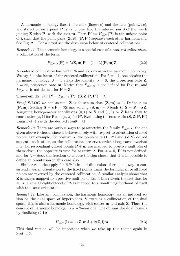
A harmonic homology fixes the center (linewise) and the axis (pointwise),and its action on a point P is as follows: find the intersection S of the line kjoining Z with P, with the axis m. Then P′ := HZ,m(P) is the unique pointof k such that the point pairs (Z,S), (P,P′) separate each other harmonically.See Fig. 2.1. For a proof see the discussion below of centered collineations.

Remark 11. The harmonic homology is a special case of a centered collineation,a collineation of the form:

PZ,m,λ(P) = λ〈Z,m〉P + (1− λ)〈P,m〉Z (2.2)

A centered collineation has center Z and axis m as in the harmonic homology.We say λ is the factor of the centered collineation. For λ = −1, one obtains theharmonic homology; λ = 1 yields the identity; λ = 0, the projection onto Z;λ = ∞, projection onto m. Notice that PZ,m,0 is not defined for P ∈ m, andPZ,m,∞ is not defined for P = Z.

Theorem 12. For P′ = PZ,m,λ(P), (S,Z; P,P′) = λ.

Proof. WLOG we can assume Z is chosen so that 〈Z,m〉 = 1. Define x :=〈P,m〉. Setting S = αP + βZ and solving 〈S,m〉 = 0 leads to S = P − xZ.Assigning homogeneous coordinates (0, 1) to S and (1, 0) to Z leads then tocoordinates (x, 1) for P and (x, λ) for P′. Evaluating the cross ratio (S,Z; P,P′)using Def. 4 yields the desired result. ut

Remark 13. There are various ways to parametrize the family PZ,m,λ; the onegiven above is chosen since it behaves nicely with respect to orientation of fixedpoints. For example, for positive λ, the point-pairs (P,P′) and (Z,S) do notseparate each other, so the collineation preserves order along each invariantline. Correspondingly, fixed points P ∈m are mapped to positive multiples ofthemselves; the opposite is true for negative λ. For λ = 0, P′ is not defined,and for λ = ±∞, the freedom to choose the sign shows that it is impossible todefine an orientation in this case also.

Similar remarks apply for RP 2n; in odd dimensions there is no way to con-sistently assign orientation to the fixed points using the formula, since all fixedpoints are reversed by the centered collineation. A similar analysis shows thatZ is always mapped to a positive multiple of itself; this reflects the fact that forall λ, a small neighborhood of Z is mapped to a small neighborhood of itselfwith the same orientation.

Remark 14. Like any collineation, the harmonic homology has an induced ac-tion on the dual space of hyperplanes. Viewed as a collineation of the dualspace, this is also a harmonic homology, with center m and axis Z. Thus, theconcept of harmonic homology is a self-dual one. One obtains the dual formulaby dualizing (2.1):

HZ,m(l) = −〈Z,m〉l + 2〈Z, l〉m (2.3)

This dual version will be important when we take up this theme again inSect. 4.6.

24

2.2 Exterior algebra

Let V be a real vector space of dimension n. The exterior, or Grassmann,algebra

∧(V), is generated by the exterior product1 ∧ applied to the vectors of

V. The exterior product is an alternating, bilinear operation. The algebra has agraded structure. The elements of grade-1 are defined to be the vectors of V; theexterior product of a k- and m-vector is a (k +m)-vector, when the operandsare linearly independent subspaces. An element that can be represented as awedge product of k 1-vectors is called a simple k-vector, or k-blade. The k-blades generate the vector subspace

∧k(V), whose elements are said to have

grade k. This subspace has dimension(nk

), hence the total dimension of the

exterior algebra is 2n.Simple and non-simple vectors. A k-blade represents the subspace of V

spanned by the k vectors which define it. Hence, the exterior algebra containswithin it a representation of the subspace lattice of V. For n > 3 there arealso k-vectors which are not blades and do not represent a subspace of V. Suchvectors occur as bivectors when V = R4 and play an important role in thediscussion of kinematics and dynamics in Chapter 8 and Chapter 9.

Dual Grassmann algebra. The same construction can be applied to con-struct

∧V∗, the exterior algebra of the dual vector space V∗. This is the algebra

of alternating k-multilinear forms.

2.2.1 Determinant function∧n(V) is a one-dimensional vector space. Let I be a basis element. Given a

basis {vi} for V, v1 ∧ v2... ∧ vn ∈∧n

(V), hence v1 ∧ v2... ∧ vn = αI for somenon-zero α ∈ R. Define a function

4 : ⊗nV→ R by 4 ({vi}) := α

Then 4 is called the determinant function of∧

(V). It lets us define a canonical

isomorphism between V and∧n−1

(V∗).

Theorem 15. V ∼=∧n−1

(V∗)

Proof. Given v ∈ V, then define ω ∈∧n−1

(V∗) by

ω(v1,v2, ...vn−1) := 4(v,v1,v2, ...,vn−1)

Conversely, given such an ω, there is a unique v such that the above equationis satisfied. Hence V ∼=

∧n−1(V∗). ut

Remark 16. By abstract nonsense, this implies V∗ ∼=∧n−1

(V).

1 Also called the outer or wedge product

25

2.2.2 Projectivized exterior algebra

The exterior algebra can be projectivized using the same process defined abovefor the construction of P (V) from V, but applied to the vector spaces

∧k(V).

This yields the projectivized exterior algebra W := P(∧

(V)). The operationsof∧

(V) carry over to P(∧V), since, roughly speaking: “Projectivization com-

mutes with outer product”. That is, for two elements X,Y ∈∧

(V):

P(X) ∧P(Y ) = P(X ∧ Y )

The difference lies in how the elements and operations are projectively inter-preted. The k-blades of P(

∧V) correspond to (k − 1)-dimensional subspaces

of P(V ). All multiples of the same k-blade represent the same projective sub-space, and differ only by intensity ([Whi98], §16-17). 1-blades correspond topoints; 2-blades to lines; 3-blades to planes, etc.

2.2.2.1 Dual exterior algebra The algebra P(∧V∗) is formed by pro-

jectivizing the dual algebra∧

(V∗). P(∧V∗) is the alternating algebra of k-

multilinear forms. By abstract nonsence, P(∧V∗) = (P(

∧V))∗: projectiviza-

tion commutes with dualization. P(∧V∗) is naturally isomorphic to P(

∧V);

again, the difference lies in how the elements and operations are interpreted.Like P(

∧V), P(

∧V∗) represents the subspace structure of P(V), but turned on

its head: 1-vectors represent projective hyperplanes, while simple (n-1)-vectorsrepresent projective points. The outer product a ∧ b corresponds to the meetrather than join operator. See also Fig. 2.4.

2.2.2.2 Notation alert In order to distinguish the two outer products ofP(∧V) and P(

∧V∗), we write the outer product in P(

∧V) as ∨, and leave

the outer product in P(∧V∗) as ∧. These symbols match closely the affiliated

operations of join (union ∪) and meet (intersection ∩), resp. Note, however,they are reversed from some modern literature ([HZ91]).

2.2.3 Exterior power of a map

Given a linear map f : V → V, there is an induced grade-preserving map∧(f) :

∧(V) →

∧(V) called the exterior power of f . Its action on a simple

k-vector a = ei1 ∧ ... ∧ eik is defined by

∧k(f) = f(ei1) ∧ ... ∧ f(eik (2.4)

For f : V → V∗, one defines a map∧

(f) :∧

(V) →∧

(V∗) by using the wedgein the dual algebra in the RHS of (2.4).

Remark 17. ∧n(f) gives the determinant of the matrix of f when f is expressedin terms of a basis {vi} satisfying 4({vi}) = 1.

26

2.2.3.1 The adjoint map Given f : V → V∗, construct the exterior power∧n−1(f) :

∧(V)→

∧(V∗). By Sect. 2.2.1,

∧n−1(f) can be considered as a map

V∗ → V. It is called the adjoint of f . We write f∗ :=∧n−1

(f). With respect toa basis, the matrix of f∗ is the “matrix of cofactors” of the matrix of f , whichisn’t surprising considering the role played in its definition by the 4 function.For invertible f , f∗ is the unique linear map satisfying 〈u,x〉 = 〈f(x), f∗(u)〉.

Remark 18. The adjoint is sometimes defined by identifying V and V∗ usinga metric. See for example [DFM07], Sec. 4.3.2. We prefer to avoid the use ofmetrics where they are not required. See related discussion in Sect. 5.10.

2.2.4 Equal rights for P(∧

V) and P(∧

V∗)

From the point of view of representing V, P(∧V) and P(

∧V∗) are equivalent.

There is no a priori reason to prefer one to the other. Every geometric elementin one algebra occurs in the other, and any configuration in one algebra has adual configuration in the other obtained by applying the Principle of Duality[Cox87], to the configuration. We refer to P(

∧V) as a point-based, and P(

∧V∗)

as a plane-based, algebra.2

Depending on the context, one or the other of the two algebras may be moreuseful. Here are some examples:

1. Joins and meets. P(∧V) is the natural choice to calculate subspace joins,

and P(∧V∗), to calculate subspace meets. See Sect. 2.3.1.4.

2. Spears and axes. Lines appear in two aspects: as spears (bivectors inP(∧V)) and axes (bivectors in P(

∧V∗)). See Sect. 2.2.4.1.

3. Euclidean geometry. P(∧V∗) is the correct choice to use for modeling

euclidean geometry. See Sect. 5.3.4. Reflections in planes. P(

∧V∗) has advantages for kinematics, since it

naturally allows building up rotations as products of reflections in planes.See Sect. 5.6.1.

We turn now to item 2 above, highlighting the importance of maintainingP(∧V) and P(

∧V∗) as equal citizens.

2.2.4.1 There are no lines, only spears and axes! Most of this workis focused on the case V = R4. In this case, bivectors are self-dual. This hasinteresting consequences for how they are interpreted.

Given two points x and y ∈ P(∧V), the condition that a third point z

lies in the subspace spanned by the 2-blade l := x ∨ y is that x ∨ y ∨ z = 0,which implies that z = αx + βy for some α, β not both zero. In projectivegeometry, such a set is called a point range. We prefer the more colorful termspear. Dually, given two planes x and y ∈ W ∗, the condition that a third

2 We prefer the dimension-dependent formulation plane-based to the more precisehyperplane-based. We also prefer not to refer to the plane-based algebra as the dualalgebra, since this formulation depends on the accident that the original algebra isinterpreted as point-based.

27

plane z passes through the subspace spanned by the 2-blade l := x ∧ y is thatz = αx + βy. In projective geometry, such a set is called a plane pencil. Weprefer the more colorful term axis.

Spear Line Axis

Fig. 2.2 Three aspects of line: spear (all incident points); line qua line; and axis (allincident planes).

Within the context of P(∧V) and P(

∧V∗), lines exist only in one of these

two aspects: of spear – as bivector in P(∧V) – and axis – as bivector in

P(∧V∗). This naturally generalizes to non-simple bivectors: there are point-

wise bivectors (in P(∧V)), and plane-wise bivectors (in P(

∧V∗).) Many of the

important operators of geometry and dynamics we will meet below, such as thepolarity on the metric quadric (Sect. 4.4), and the inertia tensor of a rigid body(Sect. 9.3), map 〈P(

∧V)〉2 to 〈P(

∧V∗)〉2 and hence map spears to axes and

vice-versa. Having both algebras on hand preserves the qualitative differencebetween these dual aspects of the generic term “line”.

Remark 19. It is possible to build up projective geometry by beginning withthe line as the primitive element and constructing points and planes from thisprimitive element. This would then provide a third way to view a line, so tospeak, in its own right rather than built out of points or planes. This approachfor example can be found in [Sto09]. But this approach does not lend itself torepresenting the subspace structure of RP 3 with Grassmann algebras.

2.3 Poincare Duality

Our treatment differs from other approaches (for example, Grassmann-Cayleyalgebras) in explicitly maintaining both algebras on an equal footing rather

28

than expressing the wedge product in one in terms of the wedge product of theother (as in the Grassman-Cayley shuffle product) ([Sel05], [Per09]). To switchback and forth between the two algebras, we construct an algebra isomorphismthat, given an element of one algebra, produces the element of the secondalgebra which corresponds to the same geometric entity of V∗.

This algebra isomorphism can be stated and proved in a coordinate-freeway using advanced techniques of modern multilinear algebra ([Gre67b], Ch.6, §2). In this form the isomorphism is called the Poincare isomorphism, andthe resulting equivalence, Poincare duality. We derive it here using a particularcoordinate system which simplifies the exposition. We first show how this worksfor the case of interest V = R4.

2.3.1 The isomorphism J

Each weighted subspace S of RP 3 corresponds to a unique element SW ofP(∧V) and to a unique element SW∗ of P(

∧V∗). We seek a bijection J :

P(∧V)↔ P(

∧V∗) such that J(SW ) = SW∗ . If we have found J for the basis

k-blades, then it extends by linearity to multivectors. This will be the desiredPoincare isomorphism. To that end, we introduce a basis for R4 and extend itto a basis for P(

∧V) and P(

∧V∗) so that J takes a particularly simple form.

Refer to Fig. 2.3.

2.3.1.1 The canonical basis A basis {e0, e1, e2, e3} of R4 corresponds to acoordinate tetrahedron for RP 3, with corners occupied by the basis elements3.Use the same names to identify the elements of P (

∧1(R4)) which correspond to

these projective points. Further, let I0 := e0 ∧ e1 ∧ e2 ∧ e3 be the basis elementof P (

∧4(R4)), and 10 be the basis element for P (

∧0(R4)). Let the basis for

P (∧2

(R4)) be given by the six edges of the tetrahedron:

Fig. 2.3 Fundamentaltetrahedron with duallabeling. Entities in Whave superscripts; entitiesin W∗ have subscripts.Planes are identified bylabeled angles of twospanning lines. A rep-resentative sampling ofequivalent elements isshown.

23 01e e=

02

31e

e=

1203

ee=

31

02

ee

=

03

12

e=

e

e3

e1

e0 e2

e1 E1=01 23e e=

e3 E3=

e0 E0=

e2 E2=

3 We use superscripts for P(∧

V) and subscripts for P(∧

V∗) since P(∧

V∗) will be themore important algebra for our purposes.

29

{e01, e02, e03, e12, e31, e23}

where eij := ei ∧ ej represents the oriented line joining ei and ej .4 Finally,choose a basis {E0,E1,E2,E3} for P (

∧3(R4)) satisfying the condition that

ei ∨ Ei = I0. This corresponds to choosing the ith basis 3-vector to be theplane opposite the ith basis 1-vector in the fundamental tetrahedron, orientedin a consistent way.

feature P(∧V) P(

∧V∗)

0-vector scalar 10 scalar 10

vector point {ei} plane {ei}bivector “spear” {eij} “axis” {eij}trivector plane {Ei} point {Ei}4-vector I0 I0

outer product join ∨ meet ∧

Table 2.1 Comparison of P(∧

V) and P(∧

V∗) for V = R4.

We repeat the process for the algebra P(∧V∗), writing indices as subscripts.

Choose the basis 1-vector ei of P(∧V∗) to represent the same plane as Ei.

That is, J(Ei) = ei. Let I0 := e0 ∧ e1 ∧ e2 ∧ e3 be the pseudoscalar of thealgebra. Construct bases for grade-0, grade-2, and grade-3 using the same rulesas above for P(

∧V) (i. e., replacing subscripts by superscripts). The results

are represented in Table 2.1.Given this choice of bases for P(

∧V) and P(

∧V∗), examination of Fig. 2.3

makes clear that, on the basis elements, J takes the following simple form:

J(ei) := Ei, J(Ei) := ei, J(eij) := ekl (2.5)

where in the last equation, (ijkl) an even permutation of (0123).Fig. 2.4 gives a graphical representation of Table 2.1, and the isomorphism

J.2.3.1.2 Description of J Furthermore, J(10) = I0 and J(I0) = 10 sincethese grades are one-dimensional. To sum up: the map J is grade-reversingand, considered as a map of coordinate-tuples, it is the identity map on allgrades except for bivectors. What happens for bivectors? In P(

∧V), consider

e01, the joining line of points e0 and e1 (refer to Fig. 2.3). In P(∧

V∗), thesame line is e23, the intersection of the only two planes which contain both ofthese points, e2 and e3. On a general bivector, J takes the form:

J(a01e01 + a02e

02 + a03e03 + a12e

12 + a31e31 + a23e

23) =

a23e01 + a31e02 + a12e03 + a03e12 + a02e31 + a01e23

4 Note that the orientation of e31 is reversed; this is traditional since Plucker introducedthese line coordinates.

30

e1

e2

e0 e0 e1e0

e0

e1

e1

e2

ΛW W*J

Λ

Fig. 2.4 The standard Grassmann P(∧

V) and its dual P(∧

V∗) are related by thePoincare isomorphism J.

The coordinate-tuple is reversed. See Fig. 2.2. This behavior is characteristicof the situation in higher dimension, to which we now turn.

2.3.1.3 J in n-dimensions Here we generalize the construction above forn = 4 to arbitrary dimension, to show how to construct the algebra isomor-phism J with the desired property, and connect it to the principle of Poincareduality. We take up the issue of J again in Sect. 5.10 where we discuss it inrelation to alternative formulations involving a metric.

A subset S = {i1, i2, ...ik} of N = {1, 2, ..., n} is called a canonical k-tupleof N if i1 < i2 < ... < ik. For each canonical k-tuple of N , define S⊥ to be thecanonical (n− k)-tuple consisting of the elements N \ S. For each unique pair{S, S⊥}, swap a pair of elements of S⊥ if necessary so that the concatenationSS⊥, as a permutation P of N , is even. Call the collection of the resulting setsS. For each S ∈ S, define eS = ei1 ...eik . We call the resulting set {eS} thecanonical basis for P(

∧V) generated by {ei}.

Consider P(∧V∗), the dual algebra to P(

∧V). Choose a basis {e1, e2, ...en}

for P(∧1 V∗) so that ei represents the same oriented subspace as the basis (n-

1)-vector e(i⊥) of P(∧V) represents. Construct the canonical basis (as above) of

P(∧V∗) generated by the basis {ei}. Then define a map J : P(

∧V)→ P(

∧V∗)

by J(eS) = eS⊥ and extend by linearity.J is an “identity” map on the subspace structure of V: it maps a simple

k-vector B ∈ W to the simple (n − k)-vector ∈ P(∧

V∗) which represents thesame geometric entity as B does in RPn. Proof: By construction, eS representsthe join of the 1-vectors eij , (ij ∈ S) in W . This is however the same subspaceas the meet of the n − k basis 1-vectors eij , (ij ∈ S⊥) of P(

∧V∗), since ei is

incident with ej ⇐⇒ j 6= i.From the construction of J we can consider it as a grade-reversing isomor-

phism P(∧V)↔ P(

∧V∗) such that J2 = id. Strictly speaking, this is the iden-

tity only projectively, in a strict vector space interpretation, J(J(X)) = ±Xfor an arbitrary k−blade X.

31

The full significance of J will only become evident after metrics are intro-duced. See Sect. 5.10.

We now show how to use J to define meet and join operators valid for bothP(∧V) and P(

∧V∗).

2.3.1.4 Projective join and meet Knowledge of J allows equal access tojoin and meet operations. We define a meet operation ∧ for two blades A,B ∈P(∧V):

A ∧B = J(J(A) ∧ J(B)) (2.6)

and extend by linearity to the whole algebra. There is a similar expression forthe join ∨ operation for two blades A,B ∈ P(

∧V∗):

A ∨B := J(J(A) ∨ J(B)) (2.7)

2.4 Remarks on homogeneous coordinates

We use the terms homogeneous model and projective model interchangeably,to denote the projectivized version of Grassmann (and, later, Clifford) algebra.

The projective model allows a certain freedom in specifying results withinthe algebra. In particular, when the calculated quantity is a subspace, then theanswer is only defined up to a non-zero scalar multiple. In some literature, thisfact is represented by always surrounding an expression x in square brackets[x] when one means “the projective element corresponding to the vector spaceelement x”. Similarly, xR is used to represent “the 1-dimensional vector sub-space corresponding to the projective point x”. We do not adhere to this levelof rigor here, since in most cases the intention is clear.

Some of the formulas introduced below take on a simpler form which takeadvantage of this freedom, but they may appear unfamiliar to those used toworking in the more strict vector-space environment. On the other hand, whenthe discussion later turns to kinematics and dynamics, then this projectiveequivalence is no longer strictly valid. Different representatives of the samesubspace represent weaker or stronger instances of a velocity or momentum(to mention two possibilities). In such situations terms such as weighted pointor “point with intensity” will be used. See [Whi98], Book III, Ch. 4. See alsoSect. 9.2.3.1 below, which discusses the use of homogeneous coordinates withrespect to the inertia tensor of a rigid body.

2.5 Guide to the literature

[PW01] (Chapter 1 and Section 2.2) provides a good overview of the backgroundmaterial on projective geometry and exterior algebra. For detailed backgroundon exterior algebras, see [Wik], [Bou89], or [Gre67b]. For more on Poincareduality, consult [Gre67b]., Sec. 6.8. [Kow09] provides a good introduction toprojective geometry with a synthetic component.

32