GALILEI GENERAL RELATIVISTIC
QUANTUM MECHANICS
ARKADIUSZ JADCZYK , MARCO M ODUGNO
Seminar of theDepartment of Applied Mathematics
University of Florence1994
Reprinted on 27.05.2002
Galilei general relativistic
quantum mechanics
Arkadiusz Jadczyk (1), Marco Modugno (2)
(1) Institute of Theoretical Physicspl. Maksa Borna 9, 50-204 Wroc-law, Poland
(2) Department of Applied Mathematics “G. Sansone”Via S. Marta 3, 50139 Florence, Italy
AbstractWe present a general relativistic approach to quantum mechanics of a spinless charged particle, subject
to external classical gravitational and electromagnetic fields in a curved space-time with absolute time.The scheme is also extended in order to treat the n-body quantum mechanics.
First, we study the Galilei general relativistic space-time, as classical background; then, we develop thequantum theory.
The formulation is fully based on geometrical ideas and methods and is explicitly covariant.In the special relativistic case, our theory agrees with the standard one referred to a given frame of ref-erence.
Our approach takes into account several classical ideas and results of Galilei general relativity and ge-ometric quantisation (see E. Cartan, C. Duval, K. Kucha®, H. P. Künzle, E. Prugovecki, A. Trautman, N.Woodhouse and several others). However, we present original ideas and results as well.
KKKKeeeeyyyy wwwwoooorrrrddddssss: Galilei general relativity, curved space-time, classical field theory, classical mechanics,quantum mechanics on a curved back-ground; fibred manifolds, jets, connections; tangent valued forms,systems.
1111999999991111 MMMMSSSSCCCC: 83D05, 81P05, 81S10, 81S40, 81T20, 70G50; 53B05, 55R05, 55R10, 58A20.
Preface
The book is addressed to a double audience: to mathematicians who atsome point were attracted by the subject of quantum mechanics, but soonwere repelled because they could not find a geometrical door to this magicpalace. It is also addressed to those physicists who knowing all kinds of culi-nary recipes of how to compute quantum mechanical effects are still unsat-isfied and thirsty of knowing some solid and primary mathematical principlesthat can be used to derive or to justify some of their successful formulae.
In fact the book is more than just a compendium building from scratch ge-ometrical foundation for Galileian relativity, wave functions, quantisationand Schrödinger equation. It is also an invitation to a further research.
The greatest unsolved problem of the XX-th century physics is as old asthe famous Einstein-Bohr debate. There were two main revolutions inphysics witnessed by this century: relativity and quantum theory. Both wereradical enough to change not only physics but also our entire Weltanschauung.After the great drama of Einstein's failure to reduce quantum theory to aunified non-linear classical field theory, after so many and so spectacularsuccesses both of relativity and quantum theory, we are tempted to believethat what we need is a union of the two opposites rather than a reduction ofone to the other. It is with this in mind that we have undertaken the researchwhose fruits we want to share in this book. We hope that perhaps our way ofapproaching quantum mechanics geometrically will trigger new ideas in somereaders, and clearly new ideas are necessary to catalyse the fruitful chemi-cal reaction between so different components.
We would like to point out the difference between our approach and that ofgeometric quantisation. Geometrical quantisation method is a powerful ma-chine feeding itself on symplectic manifolds and their polarisations. So, ithas a different scope than our approach because we are concerned withstructures related to space-time. On the other hand "time" is merely a pa-rameter in geometrical quantisation; it is never treated fully geometrically.Thus it is difficult or impossible to discuss in that framework changes of
states corresponding to accelerated observers. Our approach stresses thefull covariance from the very beginning, and covariance proves to be apowerful guiding principle.
We thank our colleagues for their interest, questions, comments and criti-cism; they allowed us to shape our research domain.
Thanks are due to Daniel Canarutto, Antonio Cassa, Christian Duval,Riccardo Giachetti, Josef Janyska, Jerzy Kijowski, Ivan Kolá®, Luca Lusanna,Peter Michor, Michele Modugno, Zbignew Oziewicz, Antonio Pérez-Rendón,Cesare Reina and Andrzej Trautman for stimulating discussions. Thanks arealso due to Raffaele Vitolo for careful reading and commenting through themanuscript.
The book came out as a result of several years of collaboration that wassupported by Italian MURST (by national and local funds) and GNFM ofConsiglio Nazionale delle Ricerche and by Polish KBN. We acknowledge theirkind support with gratitude.
Florence, 31 December 1993
Arkadiusz Jadczyk, Marco Modugno
Table of contents
0 - Introduction
0.1. Aims 40.2. Summary 60.3. Main features 190.4. Units of measurement 230.5. Further developments 24
I - The classical theory
I.1 - SPACE-TIME 25
I.1.1. Space-time fibred manifold 25I.1.2. Vertical metric 29I.1.3. Units of measurement 31
I.2 - SPACE-TIME CONNECTIONS 33
I.2.1. Space-time connections 33I.2.2. Space-time connections and observers 36I.2.3. Metrical space-time connections 38I.2.4. Divergence and codifferential operators 40I.2.5. Second order connection and contact 2-form 42I.2.6. Space-time connection 46
I.3 - GRAVITATIONAL AND ELECTROMAGNETIC FIELDS 48
I.3.1. The fields 48I.3.2. Gravitational and electromagnetic coupling 49
I.4 - FIELD EQUATIONS 55
I.4.1. First field equation 55
2 A. JADCZYK, M. MODUGNO
I.4.2. Geometrical interpretation of the first field equation 55I.4.3. First field equation interpreted through an observer 61I.4.4. First field equation interpreted through the fields 64I.4.5. Second gravitational equation 66I.4.6. Second electromagnetic equation 69I.4.7. Second field equation 71
I.5 - PARTICLE MECHANICS 73
I.5.1. The equation of motion 73I.5.2. Observer dependent formulations of the Newton law of motion 74
I.6 - SPECIAL RELATIVISTIC CASE 78
I.6.1. Affine structure of space-time 78I.6.2. Newtonian connections and the Newton law of gravitation 80I.6.3. The special relativistic space-time 85
I.7 - CLASSICAL TWO-BODY MECHANICS 87
I.7.1. Two body space-time and equations 88I.7.2. The standard two-body solution 92
II - The quantum theory
II.1 - THE QUANTUM FRAMEWORK 100
II.1.1. The quantum bundle 100II.1.2. Quantum densities 102II.1.3. Systems of connections 103II.1.4. The quantum connection 106II.1.5. Quantum covariant differentials 113II.1.6. The principle of projectability 115
II.2 - THE GENERALISED SCHRöDINGER EQUATION 117
II.2.1. The quantum Lagrangian 117II.2.2. The quantum momentum 121II.2.3. The generalised Schrödinger equation 123II.2.4. The quantum probability current 127
GALILEI GENERAL RELATIVISTIC QUANTUM MECHANICS 3
II.3 - QUANTUM VECTOR FIELDS 130
II.3.1. The Lie algebra of quantisable functions 130II.3.2. The Lie algebra of quantum vector fields 136
II.4 - QUANTUM LIE OPERATORS 143
II.4.1. Lie operators 143II.4.2. The general Lie algebras isomorphism 146II.4.3. Main examples 148
II.5 - SYSTEMS OF DOUBLE FIBRED MANIFOLDS 150
II.5.1. The system 150II.5.2. The tangent prolongation of the system 154II.5.3. Connections on the system 157
II.6 - THE INFINITE DIMENSIONAL QUANTUM SYSTEM 161
II.6.1. The quantum system 161II.6.2. The Schrödinger connection on the quantum system 162II.6.3. Quantum operators on the quantum system 164II.6.4. Commutators of quantum operators 168II.6.5. The Feynmann path integral 170
II.6 - QUANTUM TWO-BODY MECHANICS 173
II.6.1. The quantum bundle and connection over the multi-space-time 173II.6.2. The two-body solution for the quantum bundle and connection 174
III - Appendix
III.1. Fibred manifolds and bundles 177III.2. Tangent prolongation of fibred manifolds 184III.3. Jet prolongation of fibred manifolds 188III.4. Tangent valued forms 191III.5. General connections 195
IV - Indexes
IV.1 - Main symbols 200IV.2 - Analytic index 208IV.3 - References 211
4 A. JADCZYK, M. MODUGNO
La filosofia è scritta in questo grandissimo libro che conti-nuamente ci sta aperto innanzi agli occhi (io dico l'universo),ma non si puó intendere se prima non si impara a intender lalingua, e conoscer i caratteri, ne quali è scritto. Egli è scrittoin lingua matematica, e i caratteri son triangoli, cerchi ed al-tre figure geometriche, senza i quali mezzi è impossibile in-tenderne umanamente parola; senza questi è un aggirarsi vana-mente per un oscuro labirinto.
G. Galilei, VI, 232, Il Saggiatore, 1623.
0 - INTRODUCTION
0.1. Aims
The standard quantum mechanics (see, for instance, [Me], [Sk], [Sc]) isquite well established and tested, so that it must be taken as touchstone forany further development.
The supporting framework of this theory is the standard flat Galilei space-time. Moreover, an inertial frame of reference is usually assumed and theimplicit covariance of the theory is achieved by imposing a suitable transfor-mation under the action of the Galilei group.
As it is well known, the standard quantum mechanics conflicts with theclassical theory of curved space-time and gravitational field. This greatproblem is still open, in spite of several important attempts. We share theopinion that the first step aimed at approaching the solution should be ageneral relativistic formulation of quantum mechanics interacting with agiven classical gravitational field in a curved space-time.
In the physical literature, the principle of covariance is mostly formulatedin terms of representations. This viewpoint is very powerful and has beenlargely successful. Moreover, it is related to the view of geometry based onthe famous Klein's programme, hence to the theories of representation of
GALILEI GENERAL RELATIVISTIC QUANTUM MECHANICS 5
groups and Lie algebras. However, we think that the modern developments ofgeometry cannot be exhausted by this approach. Indeed, we think that a di-rect approach to geometrical structures in terms of intrinsic algebraicstructures, operators and functors is quite interesting and might deserve aprimitive consideration. Then, the groups of automorphisms of such struc-tures arise subsequently. Moreover, if the developments of the primitivestructures are derived intrinsically, through functorial methods, then the in-variance of the theory under the action of the automorphism groups is auto-matic. So, we think that, when we know the basic structures of our physicalmodel, it is worthwhile following an intrinsic, i.e. manifestly covariant, ap-proach. Indeed, in the cases when we know both an intrinsic formulation of aphysical theory and a formulation via representations, the first one appearsto be simpler and neater. Just to fix the ideas, consider a very simple exam-ple and refer to the formulations of electromagnetic field through the modernintrinsic language of exterior differential calculus and the older languagebased on components and the action of the Lorentz group. Actually, it is apity that an intrinsic geometrical language has not yet been achieved for alldomains that occur in physics. On the other hand, the method of representa-tions remains essential for the study of classifications.
So, the goal of our paper is a general relativistic quantum mechanics. Asusual, by 'general relativistic' we mean 'covariant' with respect to the changeof frames of reference (observers and units of measurement) and charts.Even more, we look for an explicitly covariant formulation based on intrinsicstructures. The reader will judge if such an approach is neat and heuristicallyvaluable.
A general relativistic quantum mechanics demands a general relativisticclassical space-time as necessary support. Certainly, the most natural andinteresting programme would be to study quantum mechanics on an Einsteingeneral relativistic back-ground, hence on a curved space-time equipped witha Lorentz metric. On the other hand, it is possible to develop a general rela-tivistic classical theory, based on a space-time fibred over absolute time andequipped with a vertical Riemannian metric. This theory - which will be re-ferred to as Galileian - is mathematically rigorous and self-contained andprovides a description of physical phenomena with a good approximation(with respect to the corresponding Einstein theory) in presence of low ve-locities and weak gravitational field. The Galilei classical mechanics has beenstudied by several authors (for instance, see [Ca], [Dv1], [Dv2], [DBKP], [DGH],
6 A. JADCZYK, M. MODUGNO
[DH], [Eh], [Ha], [Ku], [Ke1], [Ke2], [Ku], [Kü1], [Kü2], [Kü3], [Kü4], [KD], [LBL],[Le], [Ma], [Mo1], [Pl], [Pr1], [Pr2], [SP], [Tr1], [Tr2], [Tu]); nevertheless, it isnot common belief that many features, which are usually attached exclu-sively to Einstein general relativity, are also present in the Galilei theory.Then, in order to avoid confusion, we stress the difference between thegeneral validity of notions such as general relativity, curved space-timemanifold, accelerated observers, equivalence principle and so on and theirpossible specifications into an Einstein or a Galilei theory. In spite of itsweaker physical validity, the Galilei theory has some advantages due to itssimplicity. Hence, we found worth starting our approach to quantum mechan-ics from the Galilei case. Later we shall apply to the Einstein case what wehave learned in the Galilei case. On the other hand, this study can be consid-ered not only as an useful exercise in view of further developments, but alsophysically interesting by itself.
0.2. Summary
In order to help the reader to get a quick synthesis of our approach, wesketch the main ideas and steps.
0.2.1. Classical theory
We assume the classical space-time to be a 4-dimensional oriented fibredmanifold (see § III.1)
t:EEEEéTTTT
over a 1-dimensional oriented affine space associated with the vector space
T. The typical space-time chart is denoted by (x0, yi) and the corresponding
time unit of measurement by u0$T or u0$T*.
We obtain the scaled time form
dt:EEEEéTÆT*EEEE,
with coordinate expression
dt = u0æd0.
We deal with the jet space (see § III.3)
GALILEI GENERAL RELATIVISTIC QUANTUM MECHANICS 7
J1EEEEéEEEE
and the natural complementary contact maps
d:J1EEEEéT*ÆTEEEE ª:J
1EEEEéT*EEEEÆ
EEEEVEEEE,
with coordinate expressions
d = u0æd0= u0æ(Ù
0_ y
0i Ù
i) ª = ªiæÙ
i= (di - y
0i d0)æÙ
i.
A classical (absolute) motion is defined to be a section
s:TTTTéEEEE
and its (absolute) velocity is the jet prolongation
j1s:TTTTéJ
1EEEE ç T*ÆTEEEE,
with coordinate expression
j1s = u0æ⁄(Ù
0©s _ Ù
0si (Ù
i©s)^.
An observer is defined to be a section
o : EEEE é J1EEEE ç T*ÆTEEEE
and the observed velocity of the motion s is the vertical section
ıos ˆ j
1s - o©s : TTTT é T*ÆVEEEE,
with coordinate expression in an adapted chart
ıos = Ù
0si u0æ(Ù
i©s).
Vertical restrictions are denoted by “ê”.We assume space-time to be equipped with a scaled vertical Riemannian
metric
g:EEEEéAÆ(V*EEEEÆEEEEV*EEEE),
with coordinate expression
g = gijêdiæêdj g
ij$ M(EEEE,AÆ·).
The metric and the time form, along with a choice of the orientation, yield
8 A. JADCZYK, M. MODUGNO
the scaled space-time and space-like volume forms
¨:EEEEé(TÆA3/2)ÆL4T*EEEE ∆:EEEEéA3/2ÆL
3V*EEEE,
with coordinate expressions
¨ = ÊÕ¡g¡ u0æd0◊d1◊d2◊d3 ∆ = ÊÕ¡g¡ êd1◊êd2◊êd3.
Moreover, the metric yields the vertical Riemannian connection
º:VEEEEéV*EEEEÆVEEEEVVEEEE
on the fibres of space time.
There is a natural bijection between the dt-preserving torsion free linearconnections
K:TEEEEéT*EEEEÆTEEEETTEEEE
on the vector bundle TEEEEéEEEE and the torsion free affine connections
Í:J1EEEEéT*EEEEÆ
J1EEEETJ
1EEEE
on the affine bundle J1EEEEéEEEE, with coordinate expressions
K = d¬æ(Ù¬_ (K
¬ihîyh _ K
¬i0îx0) Ùî
i) Í = d¬æ(Ù
¬_ (Í
¬ihy0h _ Í
¬i©) Ù0
i)
Kµi¬= K
¬iµ= Í
¬iµ= Í
µi¬.
Then, each of such equivalent connections, will be called a space-timeconnection.
A space-time connection K yields, by vertical restriction, the space-timevertical connection
êK:VEEEEéV*EEEEÆVEEEEVVEEEE
on the fibres of space-time, with coordinate expression
êK = êdjæ(Ùj_ K
jihîyh Ùî
i).
If Í is a space-time connection and o an observer, then we obtain the co-
GALILEI GENERAL RELATIVISTIC QUANTUM MECHANICS 9
variant differential
ıo:EEEEéT*Æ(T*EEEEÆEEEEVEEEE).
Then, the vertical metric and the observer itself yield the splitting of ıointo its symmetrical and anti-symmetrical components
Á:EEEEé(T*ÆA)ÆÓ2T*EEEE È:EEEEé(T*ÆA)ÆL
2T*EEEE,
with coordinate expressions
Á ˆ - 2 u0æ(Í0j©
d0√dj _ Íij©di√dj) È ˆ - 2 u0æ(Í
0j©d0◊dj _ Í
ij©di◊dj)
The connection Í is characterised by êK, êÁ and È.A space-time connection K is said to be metrical if it preserves the con-
travariant vertical metric, i.e. if
ıKãg = 0.
We cannot fully apply the methods of Riemannian geometry, because themetric g is degenerate.
A space-time connection Í yields the connection
˙ ˆ dœÍ : J1EEEE é T*ÆTJ
1EEEE
on the fibred manifold J1EEEEéTTTT and the scaled 2-form
Ò ˆ ~Í◊ª : J
1EEEE é (T*ÆA)ÆL
2T*J
1EEEE
on the manifold J1EEEE, with coordinate expressions
˙ = u0æ⁄Ù0_ y
0i Ù
i_ (Í
hiky0h y
0k _ 2 Í
hi©y0h _ Í
0i©) Ù0
i^
Ò = giju0æ(d
0i - ˙i d0 - Í
hi ªh)◊ªj.
They are said to be, respectively, the second order connection and thecontact 2-form associated with Í.
These objects fulfill the equality
˙œÒ = 0;
moreover
10 A. JADCZYK, M. MODUGNO
dt◊Ò◊Ò◊Ò:J1EEEEé(T*2ÆA3)ÆL
7T*J
1EEEE
is a scaled volume form on J1EEEE; furthermore, for each observer o, we obtain
È = 2 o*Ò,
hence, we say that È is the observed contact 2-form.
On the other hand, ˙ and Ò characterise Í itself.
We assume space-time to be equipped with a space-time connection
ÍŸ:J1EEEEéT*EEEEÆ
J1EEEETJ
1EEEE
and a scaled 2-form
F:EEEEéBÆL2T*EEEE,
representing the gravitational connection and the electromagnetic field.The gravitational connection and the electromagnetic field can be coupled
in a natural way through a constant cccc, which can be either the square root¢Ãkkkk of the gravitational constant, or the ratio qqqq/m of a mass m$M and acharge qqqq$Q of a given particle: the coupled objects will be called total. Inpractice, we are concerned with cccc = ¢Ãkkkk only in the context of the secondgravitational field equation and in all other cases we consider cccc = qqqq/m. So,we obtain the total contact 2-form
Ò ˆ ÒŸ _ Òe ˆ ÒŸ _ 12cccc F,
the total second order connection
˙ ˆ ˙Ÿ _ ˙e
and the total space-time connection
Í ˆ ÍŸ _ Íe,
where
˙e:J1EEEEéT*Æ(T*ÆVEEEE)
turns out to be the Lorentz force and
GALILEI GENERAL RELATIVISTIC QUANTUM MECHANICS 11
Íe:J1EEEEéT*EEEEÆ
EEEE(T*ÆVEEEE)
a certain soldering form associated canonically with F, with coordinate ex-pressions
˙e = - c (F0i _ F
hi y
0h) u0æÙ
i0 Íe = 1
2c ⁄(Fi
hy0h _ 2 Fi
0) d0 _ Fi
jdj^æÙ
i0.
This splitting will be reflected in all other objects derived from the totalconnection.
In order to couple the total connection with the vertical metric, we postu-late the first field equation : for each charge and mass, the total contact 2-form is closed, i.e.
dÒ = 0.
This equation expresses, in a compact way, a large number of importantconditions. Namely, the first field equation is equivalent to the fact that thetotal connection is metrical and the total curvature tensor fulfills the stan-dard symmetry properties. Moreover, the first field equation is equivalent to
the fact that the vertical total connection êK coincides with the vertical
Riemannian connection º and, for each observer o, êÁ is given by the timederivative of the metric and È is closed. Moreover, in virtue of the arbitrari-ness of the mass and the charge, the first field equation implies the firstMaxwell equation.
In order to couple the total connection with the matter source, we postu-late the second gravitational and electromagnetic field equations :
rŸ = tŸ divŸ F = j.
We restrict ourselves to consider a charged incoherent fluid, just as an ex-ample; these equations yield an Einstein type equation for the total connec-tion
r = t.
The only observer independent way of expressing the generalised Newtonlaw of motion of a classical particle, under the action of the gravitationaland electromagnetic fields, is to assume that the covariant differential ofthe motion with respect to the second order total connection ˙ vanishes
12 A. JADCZYK, M. MODUGNO
ı j1s = 0.
We stress that the standard Hamiltonian and Lagrangian approaches toclassical dynamics depend on the choice of an observer in an essential way.Hence, they are not suitable for a general relativistic formulation of classicalmechanics.
Under reasonable hypothesis, there exist background affine structures onspace-time, which allow us to re-interpret the second field equation as theNewton law of gravitation.
In particular, the special relativistic case is obtained by considering anaffine space-time with vanishing energy tensor of matter.
By means of a slight modification of the above scheme we can formulatethe n-body field theory and mechanics on a curved Galilei space-time. In par-ticular, the standard results for the two-body classical mechanics can be re-covered as a special solution of our equations.
0.2.2. Quantum theory
We assume the quantum bundle to be a line-bundle
π:QQQQéEEEE
over space-time. The quantum histories are described by the quantum sec-tions
„:EEEEéQQQQ.
In some respects, it is useful to regard a quantum section „ as a quantumdensity
„∆ ˆ „æ¢Ã∆ : EEEE é QQQQ∆.
The typical normal chart of QQQQ will be denoted by (z) and the correspondingbase by (b); accordingly, we write
„ = ¥ b, ¥ ˆ z©„.
Then, we assume the quantum connection to be a Hermitian universal con-nection
c:QQQQŸéT*J1EEEEÆJ1EEEETQQQQŸ
GALILEI GENERAL RELATIVISTIC QUANTUM MECHANICS 13
on the pullback quantum bundle
πŸ : QQQQŸ ˆ J1EEEEEEEEQQQQ é J
1EEEE,
whose curvature is proportional to the classical total contact 2-form, ac-cording to the formula
Rc= i m
hhhhÒæi : QQQQŸ é L
2T*J
1EEEEÆJ1EEEEQQQQŸ.
The universal connection c can be naturally regarded as a system ofHermitian connections
≈:J1EEEEEEEEQQQQéT*EEEEÆ
EEEETQQQQ
on the bundle π:QQQQéEEEE, whose curvature is proportional to the observed totalcontact 2-form È, for each observer o, according to the formula
R≈o= 1
2i mhhhhÈæi : QQQQ é L
2T*EEEEÆ
EEEEQQQQ
The quantum connection is essentially our unique structure postulated forquantum mechanics; all other structures and objects will be derived fromthis in a natural way.
We prove that the coordinate expression of the quantum connection, is ofthe type
c0= - H/h c
j= p
j/h c
0j= 0,
where H and p are the classical Hamiltonian and momentum associated withthe frame of reference attached to the chosen chart, with a suitable gaugeof the total potential
a:EEEEé(T*ÆA)ÆT*EEEE
of the closed 2-form È, which refers both to the gravitational and electro-magnetic fields.
The composition
˙œc:QQQQŸéT*ÆTQQQQŸ
turns out to be a connection on the fibred manifold QQQQŸéTTTT, whose coordinateexpression is of the type
14 A. JADCZYK, M. MODUGNO
˙œc = u0æ(Ù0_ y
0i Ù
i_ ˙i Ù
i0 _ i L/h i),
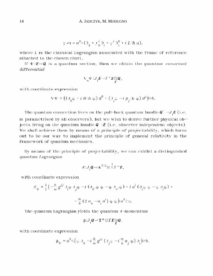
where L is the classical Lagrangian associated with the frame of referenceattached to the chosen chart.
If „:EEEEéQQQQ is a quantum section, then we obtain the quantum covariantdifferential
ıc„:J
1EEEEéT*EEEEÆ
EEEEQQQQ,
with coordinate expression
ı„ = ⁄(Ù0¥ _ i H/h ¥) d0 _ (Ù
j¥ - i p
j/h ¥) dj^æb.
The quantum connection lives on the pull-back quantum bundle QQQQŸéJ1EEEE (i.e.
is parametrised by all observers), but we wish to derive further physical ob-jects living on the quantum bundle QQQQéEEEE (i.e. observer independent objects).We shall achieve them by means of a principle of projectability, which turnsout to be our way to implement the principle of general relativity in theframework of quantum mechanics.
By means of the principle of projectability, we can exhibit a distinguishedquantum Lagrangian
L:J1QQQQéA3/2ÆL
4T*EEEE,
with coordinate expression
L„= 1
2⁄- h
mgij Ù
i㥠Ù
j¥ - i (Ù
0.㥠¥ - 㥠Ù
0.¥) _ i ai (Ù
i㥠¥ - 㥠Ù
i¥) _
_ mh(2 a
0- a
iai) 㥠¥^ u0æ¨.
The quantum Lagrangian yields the quantum 4-momentum
p:J1QQQQéT*ÆTEEEEÆ
EEEEQQQQ,
with coordinate expression
p„= u0æ⁄¥ Ù
0- i h
mgij (Ù
j¥ - i m
haj¥) Ù
i^æb.
GALILEI GENERAL RELATIVISTIC QUANTUM MECHANICS 15
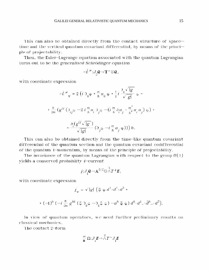
This can also be obtained directly from the contact structure of space-time and the vertical quantum covariant differential, by means of the princi-ple of projectability.
Then, the Euler-Lagrange equation associated with the quantum Lagrangianturns out to be the generalised Schrödinger equation
* êE#:J2QQQQéT*ÆQQQQ,
with coordinate expression
* êE#„= 2 ⁄i Ù
0¥ _ m
ha0¥ _ 1
2iÙ0ÊÕ¡g¡
ÊÕ¡g¡¥ _
_ h
2m(gij (Ù
ij¥ - 2 i m
haiÙj¥ - (i m
hÙiaj_ m
2
h2 ai aj) ¥) _
_Ùi(gijÊÕ¡g¡ )
ÊÕ¡g¡(Ù
j¥ - i m
haj¥))^ b.
This can also be obtained directly from the time-like quantum covariantdifferential of the quantum section and the quantum covariant codifferentialof the quantum 4-momentum, by means of the principle of projectability.
The invariance of the quantum Lagrangian with respect to the group U(1)yields a conserved probability 4-current
j:J1QQQQéA3/2ÆL
3T*EEEE,
with coordinate expression
j„= ÊÕ¡g¡ ⁄㥠¥ d1◊d2◊d3 _
_ (-1)h (- i h
2mghk (㥠Ù
k¥ - Ù
k㥠¥) - ah 㥠¥) d0◊d1…◊âdh…◊d3^.
In view of quantum operators, we need further preliminary results onclassical mechanics.
The contact 2-form
mhhhhÒ:J
1EEEEéL
2T*J
1EEEE
16 A. JADCZYK, M. MODUGNO
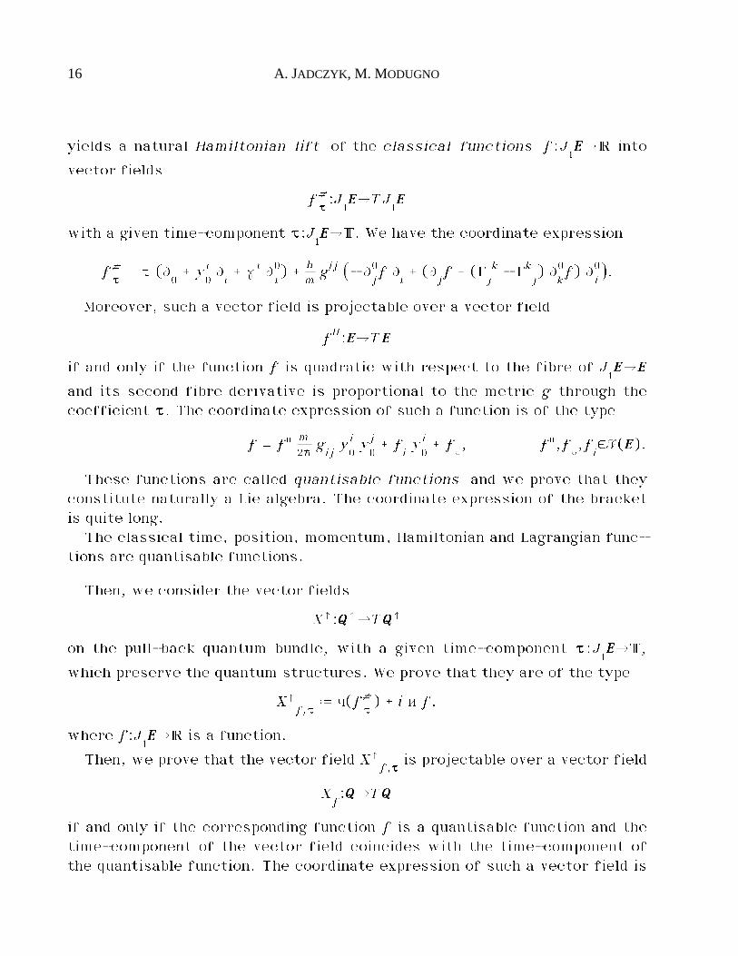
yields a natural Hamiltonian lift of the classical functions f:J1EEEEé· into
vector fields
f††††#:J
1EEEEéTJ
1EEEE
with a given time-component ††††:J1EEEEéT. We have the coordinate expression
f††††# = † (Ù
0_ y
0i Ù
i_ ˙i Ù
i0) _ h
mgij ⁄- Ù0
jf Ù
i_ (Ù
jf _ (Í
jk - Ík
j) Ù0
kf) Ù
i0^.
Moreover, such a vector field is projectable over a vector field
fH:EEEEéTEEEE
if and only if the function f is quadratic with respect to the fibre of J1EEEEéEEEE
and its second fibre derivative is proportional to the metric g through thecoefficient ††††. The coordinate expression of such a function is of the type
f = f» m2hgijy0i y
0j _ f
iy0i _ f
©, f»,f
©,f
i$F(EEEE).
These functions are called quantisable functions and we prove that theyconstitute naturally a Lie algebra. The coordinate expression of the bracketis quite long.
The classical time, position, momentum, Hamiltonian and Lagrangian func-tions are quantisable functions.
Then, we consider the vector fields
XŸ:QQQQŸéTQQQQŸ
on the pull-back quantum bundle, with a given time-component ††††:J1EEEEéT,
which preserve the quantum structures. We prove that they are of the type
XŸf,††††
ˆ c(f††††#) _ i i f,
where f:J1EEEEé· is a function.
Then, we prove that the vector field XŸf,††††
is projectable over a vector field
Xf:QQQQéTQQQQ
if and only if the corresponding function f is a quantisable function and thetime-component of the vector field coincides with the time-component ofthe quantisable function. The coordinate expression of such a vector field is
GALILEI GENERAL RELATIVISTIC QUANTUM MECHANICS 17
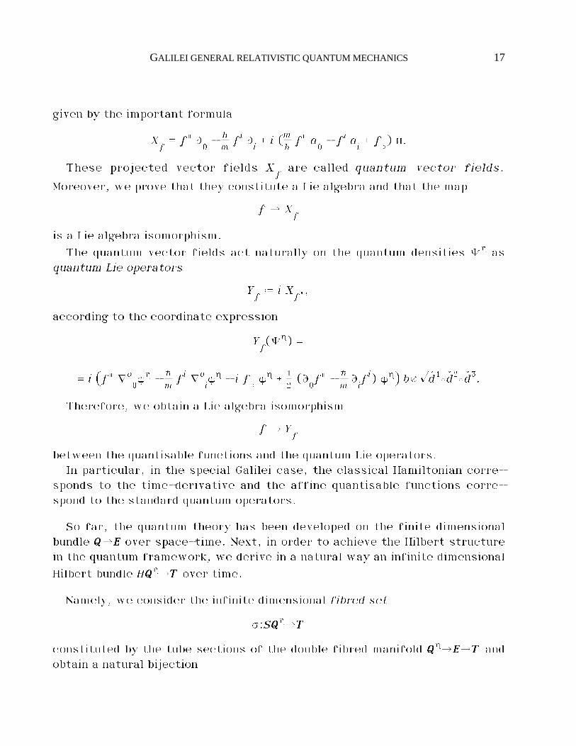
given by the important formula
Xf= f» Ù
0- h
mfi Ù
i_ i (m
hf» a
0- fi a
i_ f
©) i.
These projected vector fields Xfare called quantum vector fields.
Moreover, we prove that they constitute a Lie algebra and that the map
f ´ Xf
is a Lie algebra isomorphism.
The quantum vector fields act naturally on the quantum densities „∆ asquantum Lie operators
Yfˆ i X
f.,
according to the coordinate expression
Yf(„∆) =
= i ⁄f» ıo0¥∆ - h
mfi ıo
i¥∆ - i f
©¥∆ _ 1
2(Ù
0f» - h
mÙifi) ¥∆^ bæÊêd1◊êd2◊êd3.
Therefore, we obtain a Lie algebra isomorphism
f ´ Yf
between the quantisable functions and the quantum Lie operators.In particular, in the special Galilei case, the classical Hamiltonian corre-
sponds to the time-derivative and the affine quantisable functions corre-spond to the standard quantum operators.
So far, the quantum theory has been developed on the finite dimensionalbundle QQQQéEEEE over space-time. Next, in order to achieve the Hilbert structurein the quantum framework, we derive in a natural way an infinite dimensional
Hilbert bundle HQQQQƎTTTT over time.
Namely, we consider the infinite dimensional fibred set
ß:SQQQQ∆éTTTT
constituted by the tube sections of the double fibred manifold QQQQ∆éEEEEéTTTT andobtain a natural bijection

18 A. JADCZYK, M. MODUGNO
„´ â„
between the sections „∆:EEEEéQQQQ∆ and â„∆:TTTTéSQQQQ∆.Then, we define a smooth structure on SQQQQ∆éTTTT, according to the Frölicher's
definition of smoothness; hence, we are able to construct the tangent space
and define the connections on the fibred set SQQQQƎTTTT.The above constructions are compatible with any subsheaf of tube sections
of the double fibred manifold QQQQ∆éEEEEéTTTT; in particular, we are interested tothe tube sections with space-like compact support. They yield the fibred set
ßc:ScQQQQ∆éTTTT.
Moreover, we prove that the Schrödinger equation can be regarded as theequation
ıâkâ„∆ = 0,
where
âk:ScQQQQ∆éT*ÆTScQQQQ∆
is a symmetric connection on the infinite dimensional bundle ScQQQQ∆éTTTT, whichis called the Schrödinger connection, and has the coordinate expression
k0(„∆) = i ( h
2mêËo¥∆ _ m
ha0¥∆) u0æbæÊêd1◊êd2◊êd3.
There is a unique natural way to obtain a fibred morphism ScQQQQ∆éScQQQQ∆ over
TTTT (and not only a differential operator acting on the sections â„∆:TTTTéQQQQ∆) fromany quantisable function. Namely, the quantum operator associated with thequantisable function f is defined to be the symmetric fibred morphism
âÚf:ScQQQQ∆éScQQQQ∆
induced by the sheaf morphism
âÚfˆ âY
f- i ffff»œıâk
,
with coordinate expression
Úf(„∆) =
GALILEI GENERAL RELATIVISTIC QUANTUM MECHANICS 19
= ⁄fo¥∆ _ i 1
2(Ù
0f» - h
mÙifi) ¥∆ - i h
mfi ıo
i¥∆ - f» h
2mêËo¥∆^ bæÊêd1◊êd2◊êd3.
Thus, the above formula is our implementation of the principle of corre-spondence, achieved in a pure geometrical way.
In particular, in the special Galilei case, these operators and their commu-tators correspond to the standard ones.
Eventually, the fibred set ScQQQQƎTTTT yields the quantum Hilbert bundle
HQQQQƎTTTT,
by the completion procedure. This bundle will carry the standard probabilisticinterpretation of quantum mechanics. We stress that we do not have a uniqueHilbert space, but a Hilbert bundle over time. Indeed, a unique Hilbert spacewould be in conflict with the principle of relativity. On the other hand, aglobal observer yields an isometry between the fibres of the quantum Hilbertbundle.
The Feynmann amplitudes arise in a natural and nice way in our frame-work.
By means of a slight modification of the above scheme we can formulatethe n-body quantum mechanics on a curved Galilei space-time. In particular,the standard results for the two-body quantum mechanics can be recoveredas a special solution of our equations.
0.3. Main features
The literature concerning classical Galilei general relativity and geometricapproaches to quantum mechanics is very extended.
We have been mainly influenced by the ideas due to E. Cartan (see [Ca]), C.Duval (see [DBKP]), H. P. Künzle (see [DBKP], [Kü1], [Kü2], [Kü3]), E.Prugovecki (see [Pr]) and A. Trautman (see [Tr1], [Tr2]) and by the scheme ofgeometrical quantisation due to B. Kostant and J. M. Souriau (see [St], [Wo]).Also the papers by F. Bayen, M. Flato, C. Fronsdal, A. Lichnerowicz and D.Sternheimer (see BFFLS]), W. Pauli (see [Pl]), H. D. Dombrowski and K.Horneffer (see [DH]), P. Havas (see [Ha]), X. Kepes (see [Ke1], [Ke2]), C.Kiefer and T.P. Singh (see [KS]), K. Kucha® (see [Ku]), M. Le Bellac (see[LBL]), J. M. Levy-Leblond (see [LBL], [Le]), L. Mangiarotti (see [Ma]), M.
20 A. JADCZYK, M. MODUGNO
Modugno (see [Mo1]), E. Schmutzer and J. Plebanski (see [SP]) and W. M.Tulczyjew (see [Tu]) have been considered.
We omit a detailed comparison between the above literature and our paper,because it would take too much space. Indeed, sometimes, such a comparisonturns out to be very hard because it is not possible to recover our intrinsicand well defined spaces in other papers. We just say that our approach andresults seem to be original in several respects.
Our touchstone for quantum mechanics is the standard theory. Actually,even if our scheme is quite far from the usual one, we stress that we do nottouch the standard probabilistic interpretation and, eventually, our concreteresults agree with the standard ones in the special Galilei case. So, our the-ory can be regarded both as a generalisation of the standard theory (in orderto fulfill the principle of general relativity and to include the interaction witha gravitational field on a curved space-time) and as a new heuristic language(in view of further interpretations and developments).
All ideas and developments are achieved in a fully geometrical way. Allformulas are expressed intrinsically and their coordinate or observer depen-dent expressions are given as well.
As we have already largely discussed, groups have no direct role. On theother hand we define carefully the geometrical structures of the fundamentalspaces and derive the physical theory from them. Of course, the transfor-mation laws of the derived objects can also be checked directly.
We stress that the representations arising from our intrinsic methods arenot trivial and could not be guessed as consequence of standard procedures.In particular, our implementation of the covariant principle of correspon-dence seems to be a miracle due to these specific geometrical structures.
The principle of relativity is basically implemented by the fact that space-time is a fibred manifold, without any distinguished trivialisation. Eachsplitting of space-time is associated with an observer and no distinguishedobservers are assumed. All subsequent structures must respect this originalfeature. So, time cannot be just a trivial parameter, but the fibring over timeyields structures playing an important role in the theory.
The most usual (mostly Lagrangian or Hamiltonian) formulations of classi-
GALILEI GENERAL RELATIVISTIC QUANTUM MECHANICS 21
cal mechanics are based on the vertical tangent or cotangent spaces, or onthe cotangent space of space-time. These approaches are related to a phi-losophy, which is very far from ours; in fact, the final physical interpreta-tion of these theories cannot be expressed in an observer independent way;so, we disregard this viewpoint. Conversely, the approach based on the tan-gent space of space-time is manifestly observer independent, but it dependson the choice of a time unit of measurement. Our approach is based on the jetspace, because this is the only way to obtain a formulation which is indepen-dent of observers and units of measurement of time. Our choice yields im-portant consequences both for the classical and quantum theories.
Another, typical feature of our formulation depends on the fundamentalrole played by connections both in the classical and quantum theories. So, theclassical field theory and mechanics is based on the space-time connection;moreover, we derive the quantum dynamics and operators from the quantumconnection.
We mostly deal with linear or affine connections, but we are also con-cerned with notions and methods related to general connections (see [ MM],[Mo2], [Mo3]). As it is well known, a general connection on a fibred manifoldis defined as a section of the jet bundle; such a section can also be regarded,equivalently, as a horizontal valued 1-form on the base space, or a verticalvalued 1-form on the total space. The first viewpoint is more suitable for itsrelation with jets and the Frölicher-Nijenhuis bracket, while the second oneis more directly related to the covariant differential of forms. We refer tothe first viewpoint as the primitive one; for this reason, our coefficients ofthe connections turn out to be the negatives of the standard ones.
It is well known that the differential calculus associated with a generalconnection can be derived from the Frölicher-Nijenhuis graded Lie algebra oftangent valued forms (see [ MM], [Mo2], [Mo3]); this calculus is simple andmore powerful than the standard one, even in the case of linear connections.Therefore, we find it convenient to refer always to this general method.Indeed, some steps of our theory require specifically notions of this generalcalculus (see, for instance, the upper quantum vector fields, § II.3.2).
Classical mechanics cannot be formulated by Hamiltonian or Lagrangianapproaches in an observer independent way. On the other hand, a classicalHamiltonian (contact) formalism can be developed; however, it has no co-
22 A. JADCZYK, M. MODUGNO
variant role in classical mechanics, but yields a fundamental link betweenclassical and quantum structures, with respect to the quantum connectionand quantum operators.
Some analogies between our approach and the geometrical quantisation(see, for instance, [St], [Wo]) are evident; but also several important differ-ences arise. The main source of differences is again due to our requirementof general relativistic covariance, hence to the role of time. In particular, weare led to base the quantisation procedure on a contact 2-form; indeed thesymplectic structure of geometric quantisation is essentially vertical, hencecannot have a relativistically covariant total role.
As the vertical metric is degenerate, the standard methods of Riemanniangeometry cannot be applied fully. However, the first field equation, based onthe closure of the contact 2-form, provides a compact way of expressing thecoupling between the vertical metric and the space-time connection, andseveral other important equations as well.
The gravitational and electromagnetic coupling works well and consistentlyin all respect, in the classical and quantum theories. This seems to be anoriginal aspect of our theory.
The Lie algebra of quantisable functions is new, as far as we know. It isone of the key points of the covariant principle of correspondence.
The coordinate expression of the generalised Schrödinger equation is simi-lar to the standard one in the flat case. For short, it replaces the wavefunction with a wave density; but the difference is more subtle than it couldseem at a first insight.
We stress that, in the quantum theory, the total potential associated withan observer cannot be split into its gravitational and electromagnetic compo-nents.
The reader is only requested to have a standard knowledge of differentialgeometry, general relativity and quantum mechanics. Besides that, the workis rather self-contained.
An appendix provides a quick outline of the basic notions on fibred mani-folds, tangent and jet spaces, general connections and tangent valued forms,which are traceable only in a specialised literature. These notions are neces-
GALILEI GENERAL RELATIVISTIC QUANTUM MECHANICS 23
sary for a full understanding of all details of our treatment. However, westress that the reader, who does not like to spend too much time on an ab-stract geometrical language, does not need to go thoroughly through thissubject: a glance will be sufficient for understanding the greatest part of thepaper.
0.4. Units of measurement
A further original feature of our formulation concerns the way we treatthe units of measurement, in order to emphasise, in a clear and rigorousway, the independence of the theory from any choice of scales.
In fact, some physical objects (mass, charge, and so on) can be describedby elements of one dimensional vector spaces. Moreover, some other physicalobjects (metric, electromagnetic field, and so on) can be described by sec-tions of vector bundles, which can be identified with geometrical bundles upto a scale factor. Furthermore, each frame of reference involves a timescale.
Only ratios of two vectors of such a 1 dimensional vector space or of twoscale factors are numbers. Then, we are led to consider “semi-vector”
spaces over the “semi-field” ·_ ˆ x$· ¡ x>0 and define the dual of a semi-
vector space and the tensor products over ·_ of semi-vector spaces. In par-ticular, a vector space is also a semi-vector space and the tensor product ofa semi-vector space with a vector space turns out to be a vector space. Apositive semi-vector space is defined to be a semi-vector space whose
scalar multiplication cannot be extended neither to ·_‰0 nor to ·.When we are concerned with a 1-dimensional positive semi-vector space,
we often denote the duals of its elements as inverses and the tensor prod-ucts of its elements with vectors as scalar products; in this way, we cantreat elements of 1-dimensional positive semi-vector spaces as they werenumbers. So, our practical formulas look like the standard ones in the physi-cal literature.
We can also define the roots of 1-dimensional positive semi-vector spaces.The half-densities can be obtained as a by-product of the above algebraic
scheme.Thus, in our theory we obtain vector fields, forms, tensors and so on,
which are tensorialised with some scale factor belonging to a 1-dimensionalvector or positive semi-vector space. We stress that the usual differential
24 A. JADCZYK, M. MODUGNO
operations, such as Lie derivative, exterior differential, covariant differen-tial, and so on, can be naturally extended to the above scaled objects. Weshall perform these operations without any further warning.
0.5. Further developments
In the special relativistic Galilei case, our practical results agree with thecorresponding ones of standard quantum mechanics. For example, in thiscase, the concrete computations concerning harmonic oscillator, hydrogenatom and so on agree with the standard ones. Thus, unlike some other geo-metrical approaches to quantum mechanics, nothing needs to be checked inthis direction. Nevertheless, a possible theoretical interest of our schememight be maintained also in the special relativistic case.
Therefore, in order to provide some new concrete quantum examples on aneffectively curved space-time, one has first to find non-trivial solutions ofthe classical fields.
Eventually, we observe that our theory can be also considered from an ex-perimental viewpoint. In fact, some results could be checked in principle byexperiments. But a detailed analysis of this aspect is beyond the purpose ofthe present work.
In a forthcoming paper we shall extend our approach, preserving the spiritof the present work, in order to include spin. Moreover, we expect that ourmethods be suitable for further extension to Einstein general relativisticspace-time.
GALILEI GENERAL RELATIVISTIC QUANTUM MECHANICS 25
I - THE CLASSICAL THEORY
The general relativistic quantum theory requires a general relativisticclassical space-time as support.
Therefore, the first part of the paper is devoted to a model of Galileicurved space-time with absolute time. In this framework, we formulatethe dynamics of classical gravitational and electromagnetic fields and of aclassical test particle.
I.1 - Space-time
First, we introduce the space-time fibred manifold and its space-likemetrical structure.
I.1.1. Space-time fibred manifold
In this section, we introduce the space-time fibred manifold and studyits tangent and jet prolongations. Moreover, we state our conventionsabout coordinates.
AAAASSSSSSSSUUUUMMMMPPPPTTTTIIIIOOOONNNN CCCC1111. We assume space-time to be a 4-dimensional orientablefibred manifold (see § III.1)
t:EEEEéTTTT
over a 1-dimensional oriented affine space TTTT, associated with the vectorspace T. ò
26 A. JADCZYK, M. MODUGNO
RRRREEEEMMMMAAAARRRRKKKK IIII....1111....1111....1111. Thus, we assume the absolute time TTTT and the absolutetime function t. But we do not mention any “absolute space”, as we do notassume any distinguished splitting of the space-time fibred manifold into aproduct of time and space. Later, any choice of such a local splitting will beassociated with an observer; no distinguished observer is assumed. ò
RRRREEEEMMMMAAAARRRRKKKK IIII....1111....1111....2222. The differential of the time function is the T-valuedform
dt:EEEEéTÆT*EEEE.
We shall be involved with the tangent space TEEEE and the vertical subspaceVEEEE; we recall the exact sequence of vector bundles over EEEE (see § III.2)
0 ä V EEEEä T EEEEä
The 1-jet space J1EEEE (see § III.3) plays an important role in the classical
and quantum theories. We recall that J1EEEEéEEEE is an affine bundle associated
with the vector bundle T*ÆVEEEEéEEEE....We shall be involved with the canonical fibred morphisms over EEEE (see
[Mo2])1
d:J1EEEEéT*ÆTEEEE ª:J
1EEEEéT*EEEEÆ
EEEEVEEEE,
which provide a natural splitting of the above exact sequence over J1EEEE (they
are quoted as the contact structure of jets). ò
DDDDEEEEFFFFIIIINNNNIIIITTTTIIIIOOOONNNN IIII....1111....1111....1111. An (absolute) motion is defined to be a section
s:TTTTéEEEE
and its (absolute) velocity is defined to be its first jet prolongation
j1s:TTTTéJ
1EEEE. ¡
DDDDEEEEFFFFIIIINNNNIIIITTTTIIIIOOOONNNN IIII....1111....1111....2222. An observer is defined to be a section
o:EEEEéJ1EEEE. ¡
1d is the Cyrillic character corresponding to “d”.
GALILEI GENERAL RELATIVISTIC QUANTUM MECHANICS 27
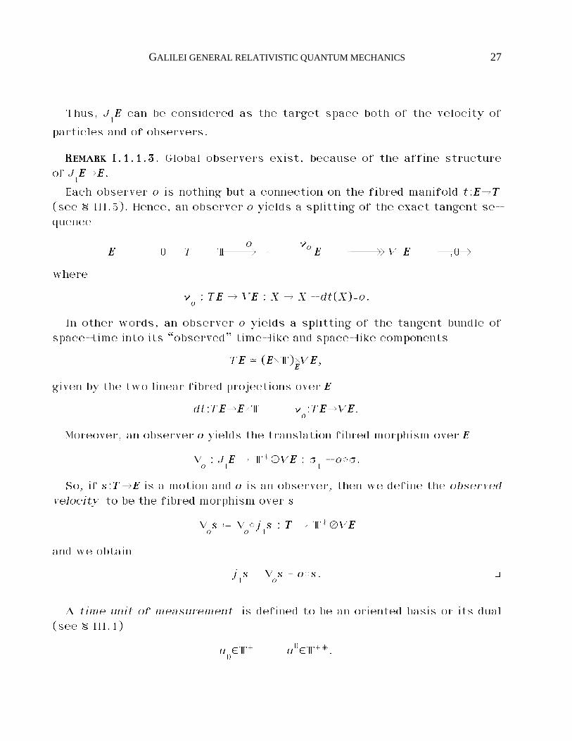
Thus, J1EEEE can be considered as the target space both of the velocity of
particles and of observers.
RRRREEEEMMMMAAAARRRRKKKK IIII....1111....1111....3333. Global observers exist, because of the affine structureof J
1EEEEéEEEE.
Each observer o is nothing but a connection on the fibred manifold t:EEEEéTTTT(see § III.5). Hence, an observer o yields a splitting of the exact tangent se-quence
0 ä EEEE˚T äo
TEEEE ä~o V EEEE ä0,
where
~o: TEEEE é VEEEE : X ´ X - dt(X)œo.
In other words, an observer o yields a splitting of the tangent bundle ofspace-time into its “observed” time-like and space-like components
TEEEE ≠ (EEEE˚T)EEEEVEEEE,
given by the two linear fibred projections over EEEE
dt:TEEEEéEEEE˚T ~o:TEEEEéVEEEE.
Moreover, an observer o yields the translation fibred morphism over EEEE
ıo: J
1EEEE é T*ÆVEEEE : ß
1- o©ß.
So, if s:TTTTéEEEE is a motion and o is an observer, then we define the observedvelocity to be the fibred morphism over s
ıos ˆ ı
o©j
1s : TTTT é T*ÆVEEEE
and we obtain
j1s = ı
os _ o©s. ò
A time unit of measurement is defined to be an oriented basis or its dual(see § III.1)
u0$T_ u0$T_*.
28 A. JADCZYK, M. MODUGNO
A frame of reference is defined to be a pair (u0, o), where u
0is a time
unit of measurement and o an observer.
We denote the typical chart of EEEE, adapted to the fibring, to a time unit of
measurement u0$T_ and to the space-time orientation, by
(x0,yi).
The induced charts of TEEEE, J1EEEE and TJ
1EEEE are denoted by
(x0,yi; îx0, îyi), (x0,yi;y0i), (x0,yi,y
0i; îx0, îyi, îy
0i).
Moreover, the corresponding local bases of vector fields and 1-forms of EEEE,TEEEE and J
1EEEE are denoted by
(Ù0,Ùi), (Ù
0,Ùi,Ùî0,Ùîi), (Ù
0,Ùi,Ù
i0) (d0,di), (d0,di,d
î0,d
îi), (d0,di,d
0i),
Thus, by construction, we have
dt©Ù0= u
0t*u0 = dx0.
Moreover, we can write
Ùi0 = u0æÙ
i.
In general, vertical restrictions will be denoted by “ê”. In particular, the
local base of vertical 1-forms of EEEE will be denoted by (êdi).Greek indices ¬, µ, … run from 0 to 3, Latin indices i,j,h,k, … run from 1 to
3 and capital Latin indices A, B, … span the values 0,1,2,3,10,20,30.
The coordinate expressions of dt, d and ª are
dt = u0ædx0
d = u0æd0
ª = ªiæÙi,
with
d0ˆ Ù
0_ y
0i Ù
iªi ˆ di - y
0i d0.
The coordinate expression of the absolute velocity of a motion s is
GALILEI GENERAL RELATIVISTIC QUANTUM MECHANICS 29
j1s = u0æ⁄(Ù
0©s _ Ù
0si (Ù
i©s)^.
Each chart (x0,yi) determines the local observer
o ˆ u0æÙ0: EEEE é T*ÆTEEEE,
with coordinate expression (in the same chart) oi0= 0. This chart is said to
be adapted to o. Conversely, each observer admits many adapted charts.Let o be an observer and let us refer to adapted coordinates. Then, we
obtain the following coordinate expressions
~o= diæÙ
iıo= yi
0u0æÙ
i;
moreover if s:TTTTéEEEE is a motion, then the coordinate expression of the ob-served velocity is
ıos = Ù
0si u0æÙ
i.
I.1.2. Vertical metric
In this section, we introduce the space-time metric and study the mainrelated structures.
AAAASSSSSSSSUUUUMMMMPPPPTTTTIIIIOOOONNNN CCCC2222. We assume space-time to be equipped with a scaled2vertical Riemannian metric
g:EEEEéAÆ(V*EEEEÆEEEEV*EEEE),
where A is a 1-dimensional positive semi-vector space (see § III.1.3). ò
Thus, A represents the space of area units.
We can also regard g as a degenerate 4-dimensional metric of signature(0,3) by considering the associated contravariant tensor
ãg : EEEE é A*Æ(VEEEEÆEEEEVEEEE) ç A*Æ(TEEEEÆ
EEEETEEEE).
The metrical linear fibred isomorphism and its inverse will be denoted by
2 Here and later, “scaled” means “defined up to a scale factor”.
30 A. JADCZYK, M. MODUGNO
g@:VEEEEéAÆV*EEEE g#:V*EEEEéA*ÆVEEEE.
The coordinate expressions of g and ãg are
g = gijêdiæêdj ãg = gij Ù
iæÙ
j
with
gij$ M(EEEE,AÆ·) gij $ M(EEEE,A*Æ·).
RRRREEEEMMMMAAAARRRRKKKK IIII....1111....2222....1111. The metric, the time-fibring and the choice of an orien-tation of the manifold EEEE yield a space-time and a space-like scaled volumeform
¨:EEEEé(TÆA3/2)ÆL4T*EEEE ∆:EEEEéA3/2ÆL
3V*EEEE.
Then, we obtain the dual elements
ã:EEEEé(T*ÆA*3/2)ÆL4TEEEE ã∆:EEEEéA*3/2ÆL
3VEEEE.
We have the coordinate expressions
¨ = ÊÕ¡g¡ u0æd0◊d1◊d2◊d3 ∆ = ÊÕ¡g¡ êd1◊êd2◊êd3
ã =1
ÊÕ¡g¡u0æÙ
0◊Ù
1◊Ù
2◊Ù
3ã∆ =
1ÊÕ¡g¡
Ù1◊Ù
2◊Ù
3,
where
¡g¡ ˆ det (gij) $ M(EEEE,A3). ò
RRRREEEEMMMMAAAARRRRKKKK IIII....1111....2222....2222. The metric g yields the Riemannian connection on the fi-bres of t:EEEEéTTTT, which can be regarded as the section
º:VEEEEéV*EEEEÆVEEEEVVEEEE,
with coordinate expression
º = êdjæ(Ùj_ º
jihîyh Ùî
i),
where
GALILEI GENERAL RELATIVISTIC QUANTUM MECHANICS 31
ºhik= - 1
2gij (Ù
hgjk_ Ù
kgjh- Ù
jghk). ò
Thus, the differences between the Einstein and Galilei general relativisticspace-times can be summarised as follows:
- in the Einstein case, we have a Lorentz metric and no fibring over abso-lute time;
- in the Galilei case, we have a “space-like” metric ãg and a “time-like” 1-
form dt:EEEEéTÆT*EEEE, which determines the fibring over absolute time.In brief words, we can say that the essential difference between the two
theories consists in the replacement of the light cones with the vertical sub-spaces.
I.1.3. Units of measurement
We have already introduced the 1-dimensional oriented vector space ofunits of measurement of time T (Ass. C1 in I.1.1) and 1-dimensional posi-tive vector space of units of measurement of area (Ass.C2 in I.1.2). Now,we complete our assumptions of fundamental spaces of units of measure-ment by introducing the 1-dimensional positive vector space of masses.
These three spaces generate all other spaces of units of measurement.In the classical theory we assume a distinguished element in one of
these spaces, namely the universal gravitational coupling constant.In the quantum theory we shall assume another distinguished element in
one of these spaces, namely the Plank constant (see Ass. Q2 in § II.1.4).
AAAASSSSSSSSUUUUMMMMPPPPTTTTIIIIOOOONNNN CCCC3333. We assume the space of masses to be a 1-dimensionalpositive semi-vector space (see § III.1.3) M. ò
The mass of a classical or quantum particle is defined to be an element
m $ M.
The mass plays the role of coupling constants for the metric.
The three fundamental 1-dimensional semi-vector spaces (see § III.1.3) T,A and M generate all spaces of units of measurement.
DDDDEEEEFFFFIIIINNNNIIIITTTTIIIIOOOONNNN IIII....1111....3333....1111. A space of units of measurement is defined to be a
32 A. JADCZYK, M. MODUGNO
1-dimensional semi-vector space of the type
U ˆ TpÆAqÆMr,
where p, q, and r are rational numbers (see § III.1.3).We say that U has dimensions
(p,q,r). ¡
In the classical theory we assume just one universal unit of measurement.
AAAASSSSSSSSUUUUMMMMPPPPTTTTIIIIOOOONNNN CCCC4444. We assume the gravitational coupling constant to be anelement
kkkk $ T*2ÆA3/2ÆM*. ò
GALILEI GENERAL RELATIVISTIC QUANTUM MECHANICS 33
I.2 - Space-time connections
In view of further development of our model, we need a preliminarystudy of connections which preserve the fibred and metrical structure ofspace-time.
I.2.1. Space-time connections
In this section, we introduce the notion of space-time connection byreferring to the tangent or to the jet space, equivalently.
RRRREEEEMMMMAAAARRRRKKKK IIII....2222....1111....1111. Let K be a linear connection on the vector bundle TEEEEéEEEE(see § III.5).
The following conditions are equivalent:i) K is dt-preserving, i.e.
ıdt = 0;
ii) the coefficients K¬0µ$F(EEEE) of K with time-like superscript vanish, i.e.
K¬0µ= 0.
Moreover, the following conditions are equivalent:iii) the fibres of t:EEEEéTTTT are auto parallel with respect to K, i.e.
ıXY $ S(VEEEEéEEEE) ÅX,Y$S(VEEEEéEEEE):
iv) K can be restricted to the fibres of t:EEEEéTTTT;v) the coefficients K
i0j$F(EEEE) of K with time-like superscript vanish, i.e.
Ki0j= 0.
Furthermore, i) implies iii). ò
Let us consider a dt-preserving torsion free linear connection
K:TEEEEéT*EEEEÆTEEEETTEEEE
34 A. JADCZYK, M. MODUGNO
on the vector bundle TEEEEéEEEE and a torsion free3 affine connection
Í:J1EEEEéT*EEEEÆ
J1EEEETJ
1EEEE,
on the affine bundle J1EEEEéEEEE.
Their coordinate expressions are of the type
K = d¬æ(Ù¬_ K
¬i Ùî
i) Í = d¬æ(Ù
¬_ Í
¬i Ù0
i)
where
K¬i ˆ K
¬ihîyh _ K
¬i0îx0 Í
¬i ˆ Í
¬ihy0h _ Í
¬i©
ͬiµ= Í
µi¬
K¬iµ= K
µi¬,
with
ͬiµ, K
¬iµ$ F(EEEE).
PPPPRRRROOOOPPPPOOOOSSSSIIIITTTTIIIIOOOONNNN IIII....2222....1111....1111. There is a natural bijection
K ´ Í
between such connections; its coordinate expression is given by
ͬiµ= K
¬iµ.
PROOF. It follows by considering the following commutative diagram
J1EEEE á á á
ÍT*EEEEÆ
EEEETJ
1EEEE
d ¸ ¸T * Æ T EEEEä
KT*Æ(T*EEEEÆ
T EEEET T EEEE )ä
≠T*EEEEÆ
TEEEET(T*ÆTEEEE) ò
DDDDEEEEFFFFIIIINNNNIIIITTTTIIIIOOOONNNN IIII....2222....1111....1111. A space-time connection is defined to be, equiva-lently, a connection K, or Í, of the above type. ¡
3 The torsion for such an affine connection is defined through the T-valuedsoldering form ª, via the Frölicher-Nijenhuis bracket (see § III.4, § III.5).
GALILEI GENERAL RELATIVISTIC QUANTUM MECHANICS 35
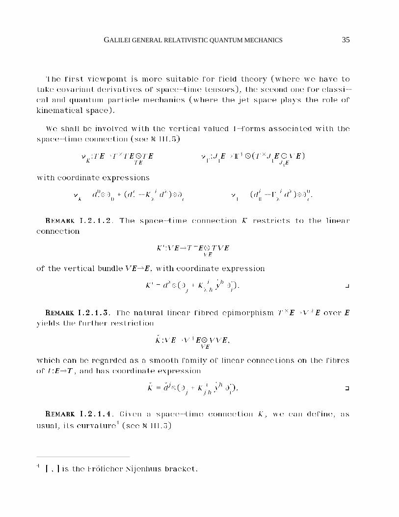
The first viewpoint is more suitable for field theory (where we have totake covariant derivatives of space-time tensors), the second one for classi-cal and quantum particle mechanics (where the jet space plays the role ofkinematical space).
We shall be involved with the vertical valued 1-forms associated with thespace-time connection (see § III.5)
~K:TEEEEéT*TEEEEÆ
TEEEETEEEE ~
Í:J1EEEEéT*Æ(T*J
1EEEEÆJ1EEEEVEEEE)
with coordinate expressions
~K= d0.æÙ
0_ (di. - K
¬i d¬)æÙ
i~Í= (di
0- Í
¬i d¬)æÙ
i0.
RRRREEEEMMMMAAAARRRRKKKK IIII....2222....1111....2222. The space-time connection K restricts to the linearconnection
K':VEEEEéT*EEEEÆVEEEETVEEEE
of the vertical bundle VEEEEéEEEE, with coordinate expression
K' = d¬æ(Ùj_ K
¬ihîyh Ùî
i). ò
RRRREEEEMMMMAAAARRRRKKKK IIII....2222....1111....3333. The natural linear fibred epimorphism T*EEEEéV*EEEE over EEEEyields the further restriction
êK:VEEEEéV*EEEEÆVEEEEVVEEEE,
which can be regarded as a smooth family of linear connections on the fibresof t:EEEEéTTTT, and has coordinate expression
êK = êdjæ(Ùj_ K
jihîyh Ùî
i). ò
RRRREEEEMMMMAAAARRRRKKKK IIII....2222....1111....4444. Given a space-time connection K, we can define, as
usual, its curvature4 (see § III.5)
4 [ , ] is the Frölicher Nijenhuis bracket.

36 A. JADCZYK, M. MODUGNO
R ˆ 12[K,K] : TEEEE é L
2T*EEEEÆ
EEEEVEEEE
its Ricci tensor
r ˆ 2 C11R : EEEE é T*EEEEÆ
EEEET*EEEE
and its scalar curvature
s ˆ Çãg, r¶ : EEEE é ·,
with coordinate expressions
R ˆ R¬µi~d¬◊dµæÙ
iæd~ = (Ù
¬Kµi~_ K
¬j~Kµij) d¬◊dµæÙ
iæd~
r = (ÙiK¬iµ- Ù
¬Kiiµ_ K
ijµK¬ij- K
¬jµKiij) d¬ædµ
s = ghk (ÙiKhik- Ù
hKiik_ K
ijhKkij- K
hjkKiij).
Then, the scalar curvature of K coincides with the scalar curvature of êK
s = ês. ò
I.2.2. Space-time connections and observers
In this section, we consider a space-time connection Í, an observer oalong with an adapted space-time chart (x0,yi) and describe the connectionthrough the observer.
RRRREEEEMMMMAAAARRRRKKKK IIII....2222....2222....1111. The covariant differential of the observer is the section
ıo:EEEEéT*Æ(T*EEEEÆEEEEVEEEE),
with coordinate expression in adapted coordinates
ıo = - u0æ(Í0i©d0 _ Í
ji©dj)æÙ
i. ò
RRRREEEEMMMMAAAARRRRKKKK IIII....2222....2222....2222. The metric g and the inclusion V*EEEE ç T*EEEE induced by theobserver allow us to regard ıo as a section
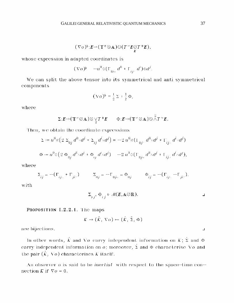
GALILEI GENERAL RELATIVISTIC QUANTUM MECHANICS 37
(ıo)@:EEEEé(T*ÆA)Æ(T*EEEEÆEEEET*EEEE),
whose expression in adapted coordinates is
(ıo)@ = - u0æ(Í0i©
d0 _ Íij©di)ædj.
We can split the above tensor into its symmetrical and anti symmetricalcomponents
(ıo)@ = 12Á _ 1
2È,
where
Á:EEEEé(T*ÆA)ÆÓ2T*EEEE È:EEEEé(T*ÆA)ÆL
2T*EEEE.
Then, we obtain the coordinate expressions
Á ˆ u0æ⁄2 Á0jd0√dj _ Á
ijdi√dj^ = - 2 u0æ(Í
0j©d0√dj _ Í
ij©di√dj)
È ˆ u0æ⁄2 È0jd0◊dj _ È
ijdi◊dj) = - 2 u0æ(Í
0j©d0◊dj _ Í
ij©di◊dj),
where
Áij= - (Í
ij©_ Í
ji©) Á
0j= - Í
0j©= È
0jÈij= - (Í
ij©- Í
ji©),
with
Á¬j, È
¬j$ M(EEEE,AÆ·). ò
PPPPRRRROOOOPPPPOOOOSSSSIIIITTTTIIIIOOOONNNN IIII....2222....2222....1111. The maps
K ´ ( êK, ıo) ´ ( êK, êÁ, È)
are bijections. ò
In other words, êK and ıo carry independent information on K; êÁ and Ècarry independent information on o; moreover, êÁ and È characterise ıo and
the pair ( êK, ıo) characterises K itself.
An observer o is said to be inertial with respect to the space-time con-nection K if ıo = 0.
38 A. JADCZYK, M. MODUGNO
Of course, inertial observers on a curved space-time might not exist at all.
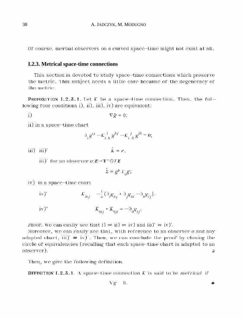
I.2.3. Metrical space-time connections
This section is devoted to study space-time connections which preservethe metric. This subject needs a little care because of the degeneracy ofthe metric.
PPPPRRRROOOOPPPPOOOOSSSSIIIITTTTIIIIOOOONNNN IIII....2222....3333....1111. Let K be a space-time connection. Then, the fol-lowing four conditions i), ii), iii), iv) are equivalent:
i) ıãg = 0;
ii) in a space-time chart
Ù¬gij - K
¬ihghj - K
¬jhgih = 0;
iii) iii)' êK = º,
iii)" for an observer o:EEEEéT*ÆTEEEE
êÁ = g@ Loãg;
iv) in a space-time chart
iv)' Kihj= - 1
2(Ù
ighj_ Ù
jghi- Ù
hgij),
iv)" K0ij_ K
0ji= - Ù
0gij.
PROOF. We can easily see that i) ∞ ii) ∞ iv) and iii)' ∞ iv)'.Moreover, we can easily see that, with reference to an observer o and any
adapted chart, iii)' ∞ iv)". Then, we can conclude the proof by closing thecircle of equivalencies (recalling that each space-time chart is adapted to anobserver). ò
Then, we give the following definition.
DDDDEEEEFFFFIIIINNNNIIIITTTTIIIIOOOONNNN IIII....2222....3333....1111. A space-time connection K is said to be metrical if
ıãg = 0. ¡
GALILEI GENERAL RELATIVISTIC QUANTUM MECHANICS 39
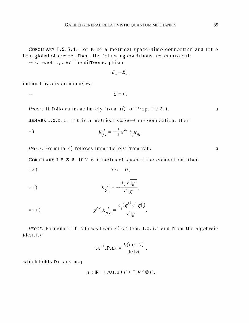
CCCCOOOORRRROOOOLLLLLLLLAAAARRRRYYYY IIII....2222....3333....1111. Let K be a metrical space-time connection and let obe a global observer. Then, the following conditions are equivalent:
- for each †,†'$TTTT the diffeomorphism
EEEE†éEEEE
†'
induced by o is an isometry;
- êÁ = 0.
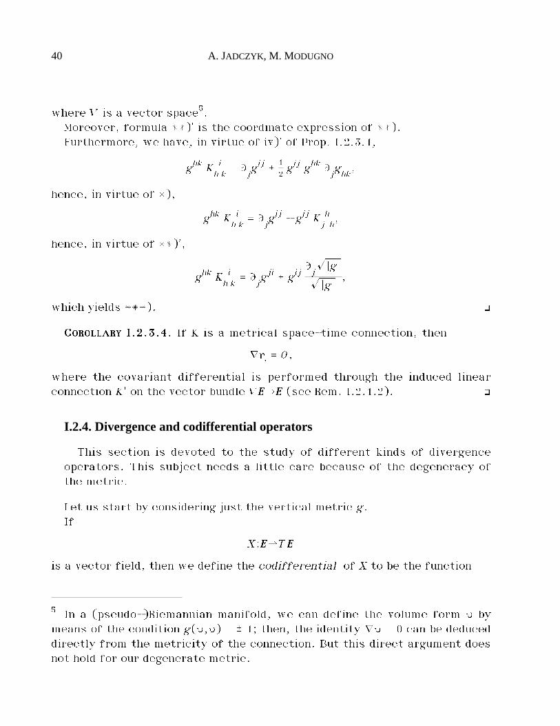
PROOF. It follows immediately from iii)" of Prop. I.2.3.1. ò
RRRREEEEMMMMAAAARRRRKKKK IIII....2222....3333....1111. If K is a metrical space-time connection, then
*) Kjii= - 1
2gih Ù
jgih.
PROOF. Formula *) follows immediately from iv)'. ò
CCCCOOOORRRROOOOLLLLLLLLAAAARRRRYYYY IIII....2222....3333....2222. If K is a metrical space-time connection, then
**) ı¨ = O;
**)' K¬ii= -
Ù¬ÊÕ¡g¡
ÊÕ¡g¡;
***) ghk Khik=Ùj(gijÊÕ¡g¡ )
ÊÕ¡g¡.
PROOF. Formula **)' follows from *) of Rem. I.2.3.1 and from the algebraicidentity
ÇA-1,DA¶ =D(detA)detA
,
which holds for any map
A : · é Auto (V) ç V*ÆV,
40 A. JADCZYK, M. MODUGNO
where V is a vector space5.Moreover, formula **)' is the coordinate expression of **).Furthermore, we have, in virtue of iv)' of Prop. I.2.3.1,
ghk Khik= Ù
jgij _ 1
2gij ghk Ù
jghk,
hence, in virtue of *),
ghk Khik= Ù
jgij - gij K
jhh,
hence, in virtue of **)',
ghk Khik= Ù
jgji _ gij
ÙjÊÕ¡g¡
ÊÕ¡g¡,
which yields ***). ò
CCCCOOOORRRROOOOLLLLLLLLAAAARRRRYYYY IIII....2222....3333....4444. If K is a metrical space-time connection, then
ı∆ = O,
where the covariant differential is performed through the induced linearconnection K' on the vector bundle VEEEEéEEEE (see Rem. I.2.1.2). ò
I.2.4. Divergence and codifferential operators
This section is devoted to the study of different kinds of divergenceoperators. This subject needs a little care because of the degeneracy ofthe metric.
Let us start by considering just the vertical metric g.If
X:EEEEéTEEEE
is a vector field, then we define the codifferential of X to be the function
5 In a (pseudo-)Riemannian manifold, we can define the volume form ¨ bymeans of the condition g(¨,¨) = — 1; then, the identity ı¨ = 0 can be deduceddirectly from the metricity of the connection. But this direct argument doesnot hold for our degenerate metric.
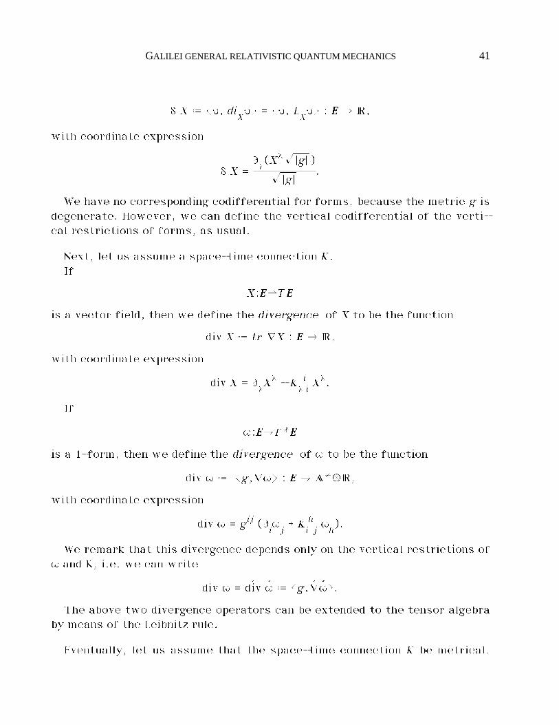
GALILEI GENERAL RELATIVISTIC QUANTUM MECHANICS 41
∂ X ˆ Çã, diX¨¶ = Çã, L
X¨¶ : EEEE é ·,
with coordinate expression
∂ X =Ù¬(X¬ÊÕ¡g¡ )
ÊÕ¡g¡.
We have no corresponding codifferential for forms, because the metric g isdegenerate. However, we can define the vertical codifferential of the verti-cal restrictions of forms, as usual.
Next, let us assume a space-time connection K.If
X:EEEEéTEEEE
is a vector field, then we define the divergence of X to be the function
div X ˆ tr ıX : EEEE é ·,
with coordinate expression
div X = Ù¬X¬ - K
¬iiX¬.
If
∑:EEEEéT*EEEE
is a 1-form, then we define the divergence of ∑ to be the function
div ∑ ˆ Çãg,ı∑¶ : EEEE é A*Æ·,
with coordinate expression
div ∑ = gij (Ùi∑j_ K
ihj∑h).
We remark that this divergence depends only on the vertical restrictions of∑ and K, i.e. we can write
div ∑ = êdiv ê∑ ˆ Çãg, êıê∑¶.
The above two divergence operators can be extended to the tensor algebraby means of the Leibnitz rule.
Eventually, let us assume that the space-time connection K be metrical.
42 A. JADCZYK, M. MODUGNO
Then we obtain the following results.If
X:EEEEéTEEEE
is a vector field, then
∂X = div X,
because the coordinate expressions of the two hand sides coincide.If
∑:EEEEéL2T*EEEE
is a 2-form, then we obtain
div2∑ = 0;
in fact div2∑ = êdiv2 ê∑ and we can apply the classical Riemannian identity.
I.2.5. Second order connection and contact 2-form
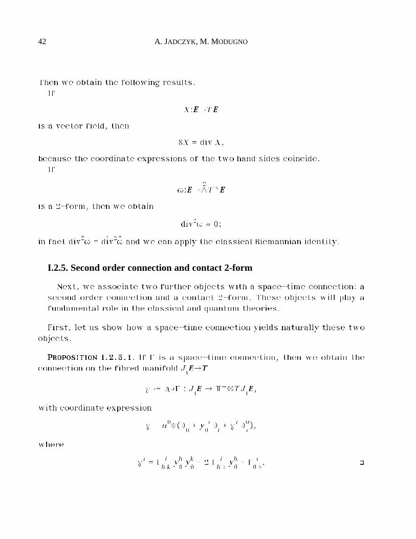
Next, we associate two further objects with a space-time connection: asecond order connection and a contact 2-form. These objects will play afundamental role in the classical and quantum theories.
First, let us show how a space-time connection yields naturally these twoobjects.
PPPPRRRROOOOPPPPOOOOSSSSIIIITTTTIIIIOOOONNNN IIII....2222....5555....1111. If Í is a space-time connection, then we obtain theconnection on the fibred manifold J
1EEEEéTTTT
˙ ˆ dœÍ : J1EEEE é T*ÆTJ
1EEEE,
with coordinate expression
˙ = u0æ(Ù0_ y
0i Ù
i_ ˙i Ù0
i),
where
˙i = Íhiky0h y
0k _ 2 Í
hi©y0h _ Í
0i©. ò
GALILEI GENERAL RELATIVISTIC QUANTUM MECHANICS 43
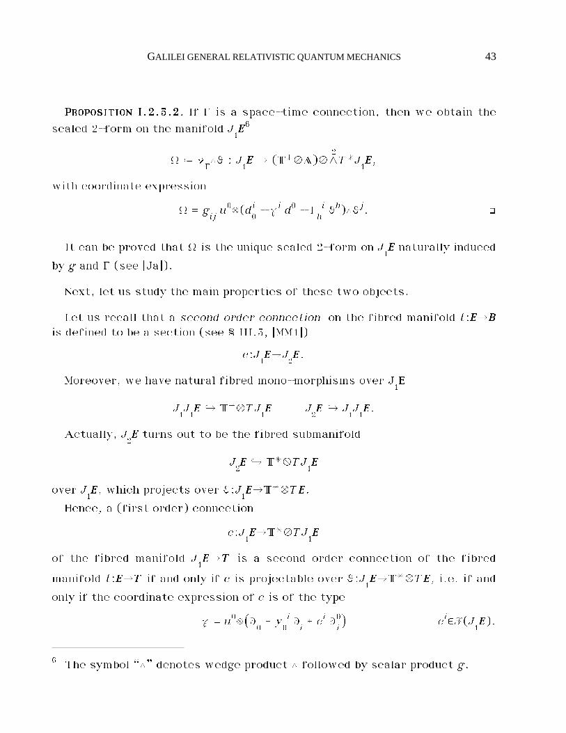
PPPPRRRROOOOPPPPOOOOSSSSIIIITTTTIIIIOOOONNNN IIII....2222....5555....2222. If Í is a space-time connection, then we obtain the
scaled 2-form on the manifold J1EEEE6
Ò ˆ ~Í◊ª : J
1EEEE é (T*ÆA)ÆL
2T*J
1EEEE,
with coordinate expression
Ò = giju0æ(d
0i - ˙i d0 - Í
hi ªh)◊ªj. ò
It can be proved that Ò is the unique scaled 2-form on J1EEEE naturally induced
by g and Í (see [Ja]).
Next, let us study the main properties of these two objects.
Let us recall that a second order connection on the fibred manifold t:EEEEéBBBBis defined to be a section (see § III.3, [MM1])
c:J1EEEEéJ
2EEEE.
Moreover, we have natural fibred mono-morphisms over J1EEEE
J1J1EEEE à T*ÆTJ
1EEEE J
2EEEE à J
1J1EEEE.
Actually, J2EEEE turns out to be the fibred submanifold
J2EEEE à T*ÆTJ
1EEEE
over J1EEEE, which projects over ª:J
1EEEEéT*ÆTEEEE.
Hence, a (first order) connection
c:J1EEEEéT*ÆTJ
1EEEE
of the fibred manifold J1EEEEéTTTT is a second order connection of the fibred
manifold t:EEEEéTTTT if and only if c is projectable over ª:J1EEEEéT*ÆTEEEE, i.e. if and
only if the coordinate expression of c is of the type
˙ = u0æ⁄Ù0_ y
0i Ù
i_ ci Ù0
i^ ci$F(J
1EEEE).
6 The symbol “◊” denotes wedge product ◊ followed by scalar product g.
44 A. JADCZYK, M. MODUGNO
Moreover, by considering the algebraic structure of the bundle J2EEEEéEEEE, we
can define the homogeneous second order connections: they are charac-
terised in coordinates by the fact that the coefficients ci are second order
polynomials in the coordinates y0j.
RRRREEEEMMMMAAAARRRRKKKK IIII....2222....5555....1111. If Í is a space-time connection, then ˙ is a homogeneous
second order connection7. ò
PPPPRRRROOOOPPPPOOOOSSSSIIIITTTTIIIIOOOONNNN IIII....2222....5555....1111. If Í is a space-time connection and o is an ob-server, then we obtain the following important equality (see § I.2.2)
È ˆ 2 o*Ò. ò
PPPPRRRROOOOPPPPOOOOSSSSIIIITTTTIIIIOOOONNNN IIII....2222....5555....2222. If Í is a space-time connection, then the 2-form Òis non-degenerate in the sense that it yields the non singular scaled volume
form8 on the manifold J1EEEE
dt◊Ò◊Ò◊Ò:J1EEEEé(T*2ÆA3)ÆL
7T*J
1EEEE. ò
PPPPRRRROOOOPPPPOOOOSSSSIIIITTTTIIIIOOOONNNN IIII....2222....5555....3333. If Í is a space-time connection, then the 2-form Òis characterised by the following property:
- for each second order connection ˙', we obtain the formula
i˙'Ò = ªœ(˙' - ˙),
with coordinate expression
i˙'Ò = g
ij(˙'i- ˙i) u0æªj.
7 If we choose a time unit of measurement u0 and replace T with ·, then thetheory of second order connections on the jet space reduces to the moreusual theory of second order differential equations on the tangent space. Ourapproach based on jets is required by the explicit independence from timeunits of measurements of our theory.8 This form can be taken as the “Liouville volume form” of our model and canbe used for developing a Galilei general relativistic statistics.
GALILEI GENERAL RELATIVISTIC QUANTUM MECHANICS 45
PROOF. It follows from a computation in coordinates, by considering the
base of forms ⁄d0, ªi, (di0- ˙i d0)^. ò
CCCCOOOORRRROOOOLLLLLLLLAAAARRRRYYYY IIII....2222....5555....1111. If Í is a space-time connection, then ˙ and Ò fulfillthe property
˙œÒ = 0. ò
So, we introduce the following definition.
DDDDEEEEFFFFIIIINNNNIIIITTTTIIIIOOOONNNN IIII....2222....5555....1111. If Í is a space-time connection, then
˙ ˆ dœÍ Ò ˆ ~Í◊ª
are said to be, respectively, the second order connection and the scaled
contact 2-form 9 associated with Í. ¡
Eventually, let us see how ˙ and Ò characterise Í.
PPPPRRRROOOOPPPPOOOOSSSSIIIITTTTIIIIOOOONNNN IIII....2222....5555....4444. If ˙ is a homogeneous second order connection onEEEEéTTTT, then there is a unique torsion free affine connection Í on J
1EEEEéEEEE, such
that
˙ = dœÍ.
PROOF. It follows from a comparison of the coordinate expressions of ˙ andÍ. ò
CCCCOOOORRRROOOOLLLLLLLLAAAARRRRYYYY IIII....2222....5555....2222. If Ò is the contact 2-form associated with thespace-time connection Í, then there is a unique connection ˙' on the fibredmanifold J
1EEEEéTTTT, such that
i˙'Ò = 0.
Namely, we have
9 In the literature, the term “contact form” is devoted to a 1-form of class2n_1 on a manifold of dimension 2n_1. So, there is no conflict between theusual terminology and ours.
46 A. JADCZYK, M. MODUGNO
˙' = ˙.
PROOF. It follows from Prop. I.2.5.3. ò
CCCCOOOORRRROOOOLLLLLLLLAAAARRRRYYYY IIII....2222....5555....3333. If Ò is the contact 2-form associated with thespace-time connection Í, then there is a unique space-time connection Í'such that
Ò = ~Í'◊ª.
Namely, we have
Í' = Í.
PROOF. It follows from Prop. I.2.5.4 and Cor. I.2.5.2. ò
We observe that, if the space-time connection is metrical, then the verti-cal restriction of the contact 2-form Ò turns out to be the vertical symplec-tic 2-form
êÒ = ~º◊Vπ
EEEE: VEEEE é AÆL
2V*VEEEE
associated with the vertical metric g. But êÒ cannot have a total role in our
theory, as a consequence of the principle of relativity. The replacement of êÒwith Ò makes an essential difference between our approach and the view-point of geometrical quantisation.
I.2.6. Space-time connections and acceleration
We conclude this section with the study of the acceleration of a motionwith respect to a given space-time connection. This subject is necessaryfor a full understanding of the meaning of the space-time second orderconnections. The results below will be used in the expression of the law ofmotion of classical particles (see § I.5.1).
Let us consider the second jet space J2EEEE (see § III.3). We recall that the
natural map J2EEEEéJ
1EEEE:ß
2´ß
1is an affine bundle associated with the vector
bundle (T*ÆT*)ÆVEEEE.
GALILEI GENERAL RELATIVISTIC QUANTUM MECHANICS 47
Now, let us consider a space-time connection Í and the associated secondorder connection ˙ (see § I.2.5).
We obtain the translation fibred morphism over J1EEEEéEEEE
ı : J2EEEE é (T*ÆT*)ÆVEEEE : ß
2´ ß
2- ˙(ß
1).
Then, let us consider a motion s:TTTTéEEEE.We define the (absolute) acceleration of s to be the second order covari-
ant differential of s, i.e. the section
ı j1s ˆ j
2s - ˙©j
1s : TTTT é (T*ÆT*)ÆVEEEE,
with coordinate expression
ı j1s = (Ù
00si - ˙i©j
1s) u0æu0æ(Ù
i©s) =
= (Ù00si - Í
hik©s Ù
0sh Ù
0sk - 2 Í
hi©©s Ù
0sh - Í
0i©©s) u0æu0æ(Ù
i©s).
48 A. JADCZYK, M. MODUGNO
I.3 - Gravitational and electromagnetic fields
So far, the space-time fibred manifold has been equipped only with thevertical metric. Now, we complete the structure of space-time by addingthe gravitational and electromagnetic fields.
I.3.1. The fields
In this section, we introduce the gravitational and electromagneticfields.
AAAASSSSSSSSUUUUMMMMPPPPTTTTIIIIOOOONNNN CCCC5555. We assume space-time to be equipped with a space-timeconnection (see § I.2.1)
ÍŸ:J1EEEEéT*EEEEÆ
J1EEEETJ
1EEEE,
and a scaled 2-form
F:EEEEéBÆL2T*EEEE,
where B is the 1-dimensional vector space
B = A1/4ÆM1/2. ò
We say that ÍŸ is the gravitational field and F the electromagnetic field .
The superscript “Ÿ” will label objects related to the gravitational connec-tion ÍŸ. In particular, we have (see § I.2.1, § I.2.5):
ıŸ ˆ ıÍŸ
˙Ÿ ˆ dœÍŸ ÒŸ ˆ ~ÍŸ◊ª.
We stress that, as the metric is degenerate, it cannot determine fully thegravitational connection. Hence, we must assume that the gravitational fieldis described just by the gravitational connection ÍŸ.
The sections s:TTTTéEEEE, which fulfill the equality
ıŸj1s = 0
GALILEI GENERAL RELATIVISTIC QUANTUM MECHANICS 49
will be interpreted as free falling motions, according to the Newton law ofmotion (see § I.5.1).
The coordinate expression of F is
F = 2 F0jd0◊dj _ F
ijdi◊dj, F
¬j$M(EEEE,BÆ·).
The (observer independent) magnetic field and electric field related toan observer o are defined to be the vertical 1-forms
B ˆ 12ê* êF : EEEE é (BÆA1/2*)ÆV*EEEE E ˆ - (oêœF) : EEEE é (T*ÆB)ÆV*EEEE
with coordinate expressions
B = ÊÕ¡g¡ (F12 êd3 _ F31 êd2 _ F23 êd1) E = Fi0êdi
and we can write
F = 2 dt◊o*(E) _ 2 o*(ê* B).
I.3.2. Gravitational and electromagnetic coupling
Next, we exhibit a natural way to incorporate the electromagnetic fieldand the gravitational connection into the geometric structures of space-time. This coupling is parametrised either by the ratio of a charge and amass or by the square root of the gravitational constant.
Such a procedure works very well both in classical and quantum theo-ries.
DDDDEEEEFFFFIIIINNNNIIIITTTTIIIIOOOONNNN IIII....3333....2222....1111. We define the space of charges to be the oriented 1-dimensional vector space
Q = T*ÆA3/4ÆM1/2. ò
The charge of a classical or quantum particle is defined to be an element
qqqq $ Q.
Moreover, given u0$T_, we set
q ˆ qqqq(u0) $ A3/4ÆM1/2.
50 A. JADCZYK, M. MODUGNO
The charge plays the role of coupling constants for the electromagneticfield.
RRRREEEEMMMMAAAARRRRKKKK IIII....3333....2222....1111. The square root of the gravitational coupling constant(see Ass. C4 in §I.1.3) and the ratio qqqq/m of any charge qqqq and mass m havethe same dimensions:
¢Ãkkkk $ T*ÆA3/4ÆM*1/2 qqqqm$ T*ÆA3/4ÆM*1/2.
Hence, the following objects have the same dimensions
ÒŸ:J1EEEEé(T*ÆA)ÆL
2T*J
1EEEE
¢Ãkkkk F:EEEEé(T*ÆA)ÆL2T*EEEE qqqq
mF:EEEEé(T*ÆA)ÆL
2T*EEEE.
Therefore, there are two distinguished ways to couple the gravitationalcontact 2-form ÒŸ and the electromagnetic field F in a way independent ofthe choice of any unit of measurement. Namely, we can use as coupling con-stant both the square root of the universal gravitational coupling constant¢Ãkkkk and the ratio qqqq/m of a given charge qqqq and a mass m. In the first case weobtain a universal coupling, in the second case the coupling depends on thechoice of a particular particle. ò
In practice, we are concerned with cccc = ¢Ãkkkk only in the context of thesecond gravitational field equation (see § I.4.5, § I.4.7) and in all other caseswe consider cccc = qqqq/m.
Thus, let us consider an element
cccc $ T*ÆA3/4ÆM*1/2,
which might be either ¢Ãkkkk, or qqqqm(for a certain given charge qqqq and mass m).
Moreover, given u0$T_, we set
c ˆ cccc(u0) $ A3/4ÆM*1/2.
We shall exhibit a natural way to deform the gravitational space-time con-nection ÍŸ, the related second order connection ˙Ÿ and contact 2-form ÒŸ
GALILEI GENERAL RELATIVISTIC QUANTUM MECHANICS 51
into corresponding “total objects ” Í, ˙ and Ò, through the electromagneticfield F.
Let us start with ÒŸ. In fact, it is natural to consider the deformed “total”2-form
Ò ˆ ÒŸ _ Òe ˆ ÒŸ _ 12cccc F,
obtained by adding the electromagnetic 2-form to the gravitational contact2-form.
Here, the coupling constant cccc is necessary for the equality of the left andright hand sides (i.e. the correct dimensionality of the above formula). Onthe other hand, we remark that we could have multiplied F by any other non-zero scalar factor; the factor 1/2 has been chosen just in order to obtain thestandard normalisation in the classical and quantum equations.
Then, we can prove the following result.
TTTTHHHHEEEEOOOORRRREEEEMMMM IIII....3333....2222....1111. Let us consider the total contact 2-form
Ò ˆ ÒŸ _ Òe ˆ ÒŸ _ 12cccc F.
Then, there exist a unique torsion free affine connection Í on the bundleJ1EEEEéEEEE and a unique connection ˙ on the fibred manifold J
1EEEEéTTTT
Í = ÍŸ _ Íe ˙ = ˙Ÿ _ ˙e
such that10
˙ ˆ dœÍ Ò ˆ ~Í◊ª ˙œÒ = 0.
Namely, ˙e turns out to be the Lorentz force
˙e ˆ - cccc g#(dêœF) : J1EEEE é T*Æ(T*ÆVEEEE)
and Íe the electromagnetic soldering form
Íe ˆ 14cccc g#⁄(ª _ 3 d)ê◊F^ : J
1EEEE é T*EEEEÆ
EEEE(T*ÆVEEEE).
10 These are just the same equalities valid for the corresponding puregravitational objects (see § I.2.5).
52 A. JADCZYK, M. MODUGNO
Moreover, the above objects fulfill the following equalities
˙e = dœÍe - Íe◊ª = Òe.
We have the coordinate expressions
˙e = - c (F0i _ F
hi y
0h) u0æÙ
i0 Íe = 1
2c ⁄(Fi
hy0h _ 2 Fi
0) d0 _ Fi
jdj^æÙ
i0,
hence
Íhik= ÍŸ
hik
Í0ik= ÍŸ
0ik_ 1
2c Fi
kÍ0i©= ÍŸ
0i©_ c Fi
0.
PROOF. The proof can be obtained by a computation in coordinates. ò
CCCCOOOORRRROOOOLLLLLLLLAAAARRRRYYYY IIII....3333....2222....1111. If o is an observer, then the gravitational and elec-tromagnetic coupling can be read in the following way
êK = êKŸ êÁ = êÁŸ È = ÈŸ _ cccc F.
PROOF. It follows from the Theor. I.3.2.1 and Prop. I.2.2.1. ò
We stress that the Lorentz force has been derived and not postulated. Thecoupling of the gravitational connection and the electromagnetic field does
not affect the torsion: both KŸ and K = KŸ _ Ke are torsion free.This coupling of the gravitational connection with the electromagnetic
field seems to be a non standard result.
RRRREEEEMMMMAAAARRRRKKKK IIII....3333....2222....1111. Suppose that the forms È, ÈŸ and F be closed and a be alocal potential of È. Then, the above splitting of È into its gravitational andelectromagnetic components does not yield an analogous distinguished split-ting of a. In fact, the potentials of È, ÈŸ and F are defined up to a gauge andit is not possible to split naturally the gauge of a into gravitational and elec-tromagnetic components. ò
CCCCOOOORRRROOOOLLLLLLLLAAAARRRRYYYY IIII....3333....2222....2222. The curvature R of the total connection K splits asfollows
R = RŸ _ RŸe_ Re,
where
GALILEI GENERAL RELATIVISTIC QUANTUM MECHANICS 53
RŸ ˆ 12[KŸ,KŸ]
is the standard gravitational curvature and the other two terms are given by
RŸe ˆ dŸKe ˆ [KŸ,Ke] Re ˆ [Ke,Ke].
We have the following coordinate expressions
RŸ ˆ RŸ¬µi~d¬◊dµæÙ
iæd~ = (Ù
¬KŸ
µi~_ KŸ
¬j~KŸ
µij) d¬◊dµæÙ
iæd~
RŸe = 12c ⁄⁄(ıŸ
0Fkj- 2 ıŸ
jFk0) îx0 - ıŸ
jFkhîyh^ d0◊dj _ ıŸ
iFkjîx0 di◊dj^æÙ
k
Re = 14c2 Fh
jFihdj◊d0æÙ
iæd0.
PROOF. We have (see § III.5 and § III.4)
R = 12[K,K] = 1
2[KŸ,KŸ] _ 1
2[KŸ,Ke] _ 1
2[Ke,KŸ] _ 1
2[Ke,Ke].
Moreover, we can write (see § III.4)
[KŸ,Ke] = [Ke,KŸ]. ò
CCCCOOOORRRROOOOLLLLLLLLAAAARRRRYYYY IIII....3333....2222....4444. The Ricci tensor r of the total connection K splits asfollows
r = rŸ _ rŸe_ re,
where
rŸ ˆ 2 C11RŸ
is the standard gravitational Ricci tensor and the other two terms are givenby
rŸe ˆ 12cccc (dtædivŸ F _ divŸ Fædt) re ˆ - 1
4êF2 cccc2 dtædt,
where
êF2 ˆ (g#æg#)©êF œ êF : EEEEéA*3/2ÆM.
We have the following coordinate expressions
54 A. JADCZYK, M. MODUGNO
rŸe = 12c ı
kFk¬(d0æd¬ _ d¬æd0) re = - 1
4c2 F
ijFij d0æd0. ò
CCCCOOOORRRROOOOLLLLLLLLAAAARRRRYYYY IIII....3333....2222....5555. The scalar curvature s of the total connection K isjust the scalar curvature of the gravitational connection
s = sŸ = êsŸ. ò
GALILEI GENERAL RELATIVISTIC QUANTUM MECHANICS 55
I.4 - Field equations
Now, we introduce the gravitational and electromagnetic field equations.We consider two equations: the first one couples just the gravitational andelectromagnetic fields, while the second one couples the gravitational andelectromagnetic fields with the charged matter sources.
I.4.1. First field equation
The first field equation is expressed through the closure of the totalcontact 2-form.
This equation turns out to be a compact way to express several impor-tant conditions involving the classical fields. Moreover, it could be used toformulate the inverse Lagrangian problem of dynamics (for the trivialcase, see, for instance, [Cr], [CPT]). Furthermore, it will occur as an es-sential integrability condition in the quantum theory (see § II.1.4).
AAAASSSSSSSSUUUUMMMMPPPPTTTTIIIIOOOONNNN CCCC6666. (First field equation) We assume that, for any couplingconstant cccc, the total contact 2-form Ò is closed, i.e.
dÒ = 0 Å cccc $ T*ÆA3/4ÆM*1/2. ò
We stress that there is no canonical local potential of Ò even in the case
when the space-time connection is flat11.
We can interpret the above equation in several interesting ways.
I.4.2. Geometrical interpretation of the first field equation
The first field equation says that, for each coupling constant cccc, the to-
11 In a sense, in the quantum framework, we shall postulate a distinguishedpotential of Ò, after adding a complex dimension to space-time through thequantum bundle QQQQéEEEE.
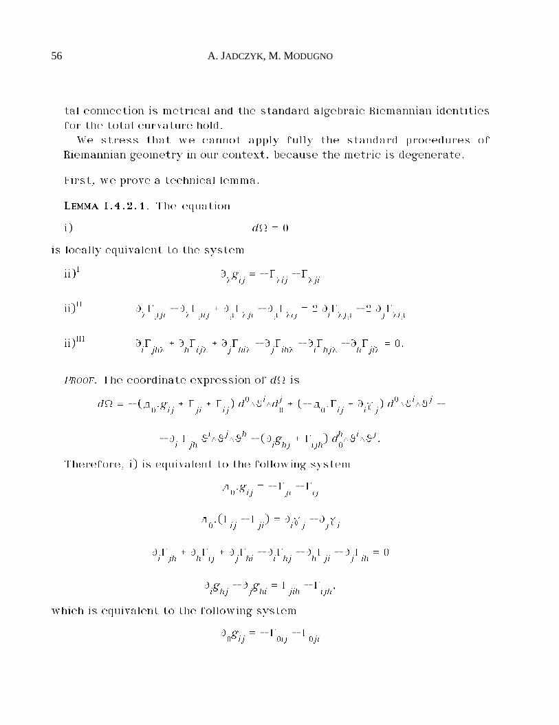
56 A. JADCZYK, M. MODUGNO
tal connection is metrical and the standard algebraic Riemannian identitiesfor the total curvature hold.
We stress that we cannot apply fully the standard procedures ofRiemannian geometry in our context, because the metric is degenerate.
First, we prove a technical lemma.
LLLLEEEEMMMMMMMMAAAA IIII....4444....2222....1111. The equation
i) dÒ = 0
is locally equivalent to the system
ii)I Ù¬gij= - Í
¬ij- Í
¬ji
ii)II ٬͵ji
- ٬͵ij
_ ٵͬji
- ٵͬij
= 2 Ùiͬjµ
- 2 Ùjͬiµ
ii)III ÙiÍjh¬
_ ÙhÍij¬
_ ÙjÍhi¬
- ÙjÍih¬
- ÙiÍhj¬
- ÙhÍji¬= 0.
PROOF. The coordinate expression of dÒ is
dÒ = - (d0.g
ij_ Í
ji_ Í
ij) d0◊ªi◊dj
0_ (- d
0.Í
ij_ Ù
i˙j) d0◊ªi◊ªj -
- ÙiÍjhªi◊ªj◊ªh - (Ù
ighj_ Í
ijh) d
0h׻i׻j.
Therefore, i) is equivalent to the following system
d0.g
ij= - Í
ji- Í
ij
d0.(Í
ij- Í
ji) = Ù
i˙j- Ù
j˙i
ÙiÍjh_ Ù
hÍij_ Ù
jÍhi- Ù
iÍhj- Ù
hÍji- Ù
jÍih= 0
Ùighj- Ù
jghi= Í
jih- Í
ijh,
which is equivalent to the following system
Ù0gij= - Í
0ij- Í
0ji
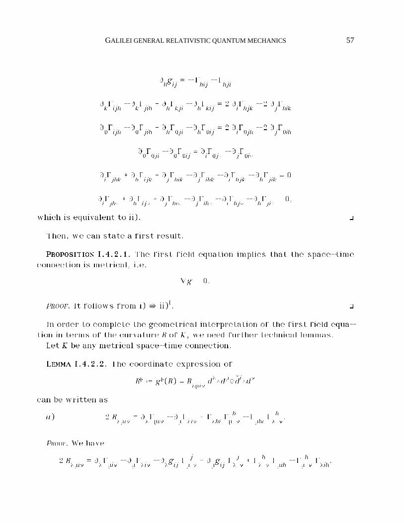
GALILEI GENERAL RELATIVISTIC QUANTUM MECHANICS 57
Ùhgij= - Í
hij- Í
hji
ÙkÍijh- Ù
kÍjih_ Ù
hÍkji- Ù
hÍkij= 2 Ù
iÍhjk
- 2 ÙjÍhik
Ù0Íijh- Ù
0Íjih_ Ù
hÍ0ji- Ù
hÍ0ij= 2 Ù
iÍ0jh
- 2 ÙjÍ0ih
Ù0Í0ji- Ù
0Í0ij= Ù
iÍ0j©
- ÙjÍ0i©
ÙiÍjhk
_ ÙhÍijk_ Ù
jÍhik
- ÙjÍihk
- ÙiÍhjk
- ÙhÍjik= 0
ÙiÍjh©
_ ÙhÍij©_ Ù
jÍhi©
- ÙjÍih©
- ÙiÍhj©
- ÙhÍji©= 0,
which is equivalent to ii). ò
Then, we can state a first result.
PPPPRRRROOOOPPPPOOOOSSSSIIIITTTTIIIIOOOONNNN IIII....4444....2222....1111. The first field equation implies that the space-timeconnection is metrical, i.e.
ıãg = 0.
PROOF. It follows from i) £ ii)I. ò
In order to complete the geometrical interpretation of the first field equa-tion in terms of the curvature R of K, we need further technical lemmas.
Let K be any metrical space-time connection.
LLLLEEEEMMMMMMMMAAAA IIII....4444....2222....2222. The coordinate expression of
R@ ˆ g@(R) = R¬µi~
d¬◊dµæêdi◊d~
can be written as
a) 2 Rµi~
= ٬͵i~
- ٵͬi~
_ ͬhi
͵h~- Í
µhiͬh~.
PROOF. We have
2 Rµi~
= ٬͵i~
- ٵͬi~
- Ù¬gij͵j~_ Ù
µgijͬj~_ Í
¬h~͵ih
- ͵h~ͬih.
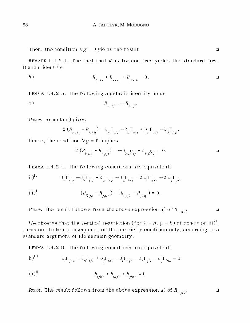
58 A. JADCZYK, M. MODUGNO
Then, the condition ıãg = 0 yields the result. ò
RRRREEEEMMMMAAAARRRRKKKK IIII....4444....2222....1111. The fact that K is torsion free yields the standard firstBianchi identity
b) Rµi~
_ R~¬iµ
_ Rµ~i¬
= 0. ò
LLLLEEEEMMMMMMMMAAAA IIII....4444....2222....3333. The following algebraic identity holds
c) Rµij
= - Rµji
.
PROOF. Formula a) gives
2 (Rµij
_ Rµji
) = ٬͵ij
- ٵͬij
_ ٬͵ji
- ٵͬji.
Hence, the condition ıãg = 0 implies
2 (Rµij
_ Rµji
) = - Ù¬µgij_ Ù
¬µgji= 0. ò
LLLLEEEEMMMMMMMMAAAA IIII....4444....2222....4444. The following conditions are equivalent:
ii)II Ù¬Íijµ
- Ù¬Íjiµ
_ ٵͬji
- ٵͬij
= 2 Ùi͵j¬
- 2 Ùj͵i¬
iii)I (Ri¬jµ
- Rjµi¬
) _ (Riµj¬
- Rj¬iµ
) = 0.
PROOF. The result follows from the above expression a) of Rµi~
. ò
We observe that the vertical restriction (for ¬ = h, µ = k) of condition iii)I,turns out to be a consequence of the metricity condition only, according to astandard argument of Riemannian geometry.
LLLLEEEEMMMMMMMMAAAA IIII....4444....2222....5555. The following conditions are equivalent:
ii)III ÙiÍjh¬
_ ÙhÍij¬
_ ÙjÍhi¬
- ÙiÍhj¬
- ÙhÍji¬
- ÙjÍih¬
= 0
iii)II Rijh¬
_ Rhij¬
_ Rjhi¬
= 0.
PROOF. The result follows from the above expression a) of Rµi~
. ò
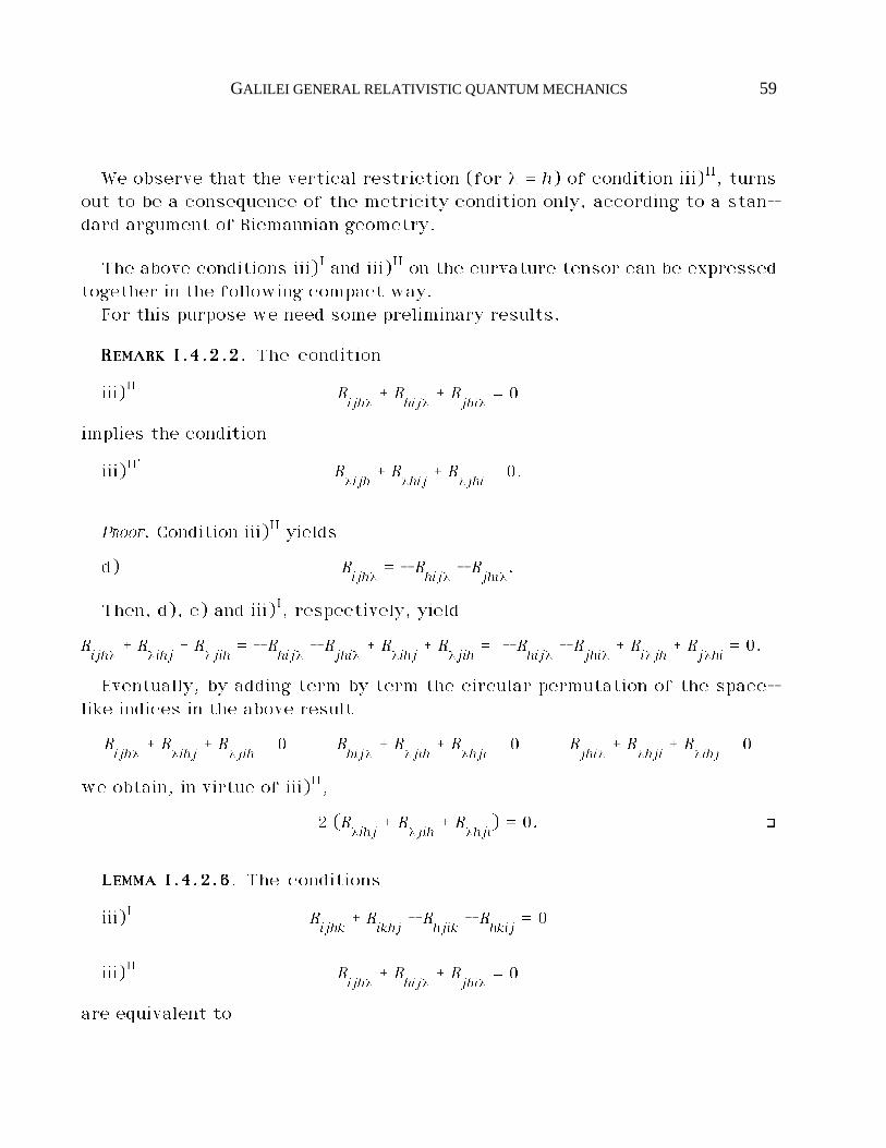
GALILEI GENERAL RELATIVISTIC QUANTUM MECHANICS 59
We observe that the vertical restriction (for ¬ = h) of condition iii)II, turnsout to be a consequence of the metricity condition only, according to a stan-dard argument of Riemannian geometry.
The above conditions iii)I and iii)II on the curvature tensor can be expressedtogether in the following compact way.
For this purpose we need some preliminary results.
RRRREEEEMMMMAAAARRRRKKKK IIII....4444....2222....2222. The condition
iii)II Rijh¬
_ Rhij¬
_ Rjhi¬
= 0
implies the condition
iii)II' R¬ijh
_ R¬hij
_ R¬jhi
= 0.
PROOF. Condition iii)II yields
d) Rijh¬
= - Rhij¬
- Rjhi¬
.
Then, d), c) and iii)I, respectively, yield
Rijh¬
_ R¬ihj
_ R¬jih
= - Rhij¬
- Rjhi¬
_ R¬ihj
_ R¬jih
= - Rhij¬
- Rjhi¬
_ Ri¬jh
_ Rj¬hi
= 0.
Eventually, by adding term by term the circular permutation of the space-like indices in the above result
Rijh¬
_ R¬ihj
_ R¬jih
= 0 Rhij¬
_ R¬jih
_ R¬hji
= 0 Rjhi¬
_ R¬hji
_ R¬ihj
= 0
we obtain, in virtue of iii)II,
2 (R¬ihj
_ R¬jih
_ R¬hji
) = 0. ò
LLLLEEEEMMMMMMMMAAAA IIII....4444....2222....6666. The conditions
iii)I Rijhk
_ Rikhj
- Rhjik
- Rhkij
= 0
iii)II Rijh¬
_ Rhij¬
_ Rjhi¬
= 0
are equivalent to
60 A. JADCZYK, M. MODUGNO
iii)R Ri¬jµ
= Rjµi¬
.
PROOF. Let us prove that iii)I, iii)II £ iii)R. Identities iii)II', c) and b), respec-tively, yield
Ri¬jh
= - R¬ijh
= R¬hij
_ R¬jhi
= R¬hij
_ Rj¬ih
= - Rhji¬
= Rjhi¬
,
hence
Ri¬jh
= Rjhi¬
.
Moreover, iii)I implies
Ri0j0
= Rj0i0
.
Now, let us prove that iii)R £ iii)I, iii)II. We can see immediately that iii)R
£ iii)I. Next, condition iii)R and identities c) and b), respectively, yield
Rijh¬
_ Rhij¬
_ Rjhi¬
= Rh¬ij
_ Rj¬hi
_ Rjhi¬
= - R¬hij
- Rj¬ih
_ Rhji¬
= 0. ò
Then, we can state a second result.
PPPPRRRROOOOPPPPOOOOSSSSIIIITTTTIIIIOOOONNNN IIII....4444....2222....2222. The first field equation implies the identity
R i¬jµ= R j
µi¬.
PROOF. It follows from i) £ iii)II, iii)III. ò
The two above results can be joined to provide a first geometrical inter-pretation of the first field equation.
TTTTHHHHEEEEOOOORRRREEEEMMMM IIII....4444....2222....1111. The first field equation is equivalent to the system
ıãg = 0 R i¬jµ= R j
µi¬.
PROOF. It follows from i) ∞ ii)II, ii)III. ò
GALILEI GENERAL RELATIVISTIC QUANTUM MECHANICS 61
I.4.3. First field equation interpreted through an observer
We can exhibit another interesting interpretation of the first field equa-tion in terms of the vertical restriction of the total connection and thetotal symmetric 2-tensor and 2-form associated with an observer.
We have a first immediate result.
PPPPRRRROOOOPPPPOOOOSSSSIIIITTTTIIIIOOOONNNN IIII....4444....3333....1111. The first field equation implies that the verticalrestriction of K is just the vertical Riemannian connection (see Rem. I.1.2.2)
êK = º .
PROOF. The condition ii)I yields
iv)I êKhik
ˆ Khik
= - 12(Ù
hgik_ Ù
kgih- Ù
ighk) = º
hik. ò
Now, we refer to the tensors Á and È related to a given observer o and toadapted coordinates (see § I.2.2).
Then, we have a second immediate result.
PPPPRRRROOOOPPPPOOOOSSSSIIIITTTTIIIIOOOONNNN IIII....4444....3333....2222. The first field equation implies that the verticalrestriction of the tensor Á is determined by the metric, according to theequation (see formula iii)" in Prop. I.2.3.1)
êÁ = g@ Loãg,
where L0is the Lie derivative with respect to the observer o, i.e. in adapted
coordinates
iv)II Áij= Ù
0gij.
PROOF. It follows from ii)I. ò
In order to complete our interpretation, we need some technical lemmas.
LLLLEEEEMMMMMMMMAAAA IIII....4444....3333....1111. If iv)I and iv)II hold, then, the two following conditions areequivalent:
62 A. JADCZYK, M. MODUGNO
iii)IV Ù0Íijh- Ù
0Íjih_ Ù
hÍ0ji- Ù
hÍ0ij= 2 Ù
iÍ0jh
- 2 ÙjÍ0ih
iv)III ÙhÈij_ Ù
jÈhi_ Ù
iÈjh= 0. ò
LLLLEEEEMMMMMMMMAAAA IIII....4444....3333....2222. If iv)II holds, then the two following conditions areequivalent:
iii)VII ÙiÍ0jh
_ ÙhÍ0ij_ Ù
jÍ0hi
- ÙiÍ0hj
- ÙhÍ0ji- Ù
jÍ0ih
= 0
iv)III ÙhÈij_ Ù
jÈhi_ Ù
iÈjh= 0. ò
LLLLEEEEMMMMMMMMAAAA IIII....4444....3333....3333. If iv)II holds, then the two following conditions areequivalent:
iii)V Ù0Í0ji- Ù
0Í0ij= Ù
iÍ0j©
- ÙjÍ0i©
iv)IV Ù0Èij= Ù
iÈ0j- Ù
jÈ0i. ò
Then we have a third result.
PPPPRRRROOOOPPPPOOOOSSSSIIIITTTTIIIIOOOONNNN IIII....4444....3333....3333. The first field equation implies that the form È isclosed
dÈ = 0.
PROOF. It follows from i) £ iv)I, iv)III, iv)IV. ò
The three above results can be joined to provide a second geometrical in-terpretation of the first field equation.
TTTTHHHHEEEEOOOORRRREEEEMMMM IIII....4444....3333....1111. Given an observer o, the first field equation is equiva-lent to the following conditions:
- the (observer independent) vertical restriction of K coincides with thevertical Riemannian connection
êK = º,
GALILEI GENERAL RELATIVISTIC QUANTUM MECHANICS 63
i.e. in coordinates
Khik
= - 12(Ù
hgik_ Ù
kgih- Ù
ighk);
- the vertical restriction of the tensor Á is determined by the metric, ac-cording to the equation (see formula iii)" in Prop. I.2.3.1)
êÁ = g@ Loãg,
where L0is the Lie derivative with respect to the observer, i.e. in adapted
coordinates
K0ij_ K
0ji= - Ù
0gij;
- the form È is closed
dÈ = 0,
i.e. in adapted coordinates
(Ù0Èij- 2 Ù
iÈ0j) d0◊di◊dj _ Ù
hÈijdh◊di◊dj =
= 2 ⁄(Ù0Í0ij_ Ù
iÍ0j0) d0◊di◊dj _ Ù
hÈijdh◊di◊dj^ = 0.
PROOF. It follows from i)∞ iv)I, iv)II, iv)III, iv)IV. ò
Of course, we might have deduced immediately dÈ = 0 from dÒ = 0 because
the pullback o* commutes with d; but in order to prove the rest, it is neces-sary to consider the above lemmas dealing with coordinate formulas.
We recall that any space-time connection K is characterised by its vertical
restriction êK and the tensors êÁ and È related to a given observer (see Prop.I.2.2.1). Hence, we have proved that K is determined by the first jet of themetric g and by an observer dependent closed 2-form È.
The above result can be re-formulated as follows.
TTTTHHHHEEEEOOOORRRREEEEMMMM IIII....4444....3333....2222. Let
a:EEEEé(T*ÆA)ÆT*EEEE
64 A. JADCZYK, M. MODUGNO
be a local potential of the closed 2-form È, i.e. a local solution of the equa-tion
È = 2 da,
with coordinate expression
Ȭµ= Ù
¬aµ- Ù
µa¬,
where
a ˆ a¬u0æd¬.
Then, the coordinate expression of the total connection can be written as
K¬iµ
= - 12(Ù
¬giµ_ Ù
µgi¬- Ù
igµ),
where we have set
gi0ˆ g
0iˆ a
ig00ˆ 2 a
0. ò
Thus, as in the Einstein theory, the space-time connection is obtained lo-cally from 10 scalar potentials; in the Galilei theory, only 6 potentials are thecomponents of the metric g and we have 4 additional potentials. This differ-ence between the Galilei and the Einstein theories is related to the fact that,in the Galilei case, g is degenerate.
We stress that the total potential a involves both the gravitational andelectromagnetic fields.
I.4.4. First field equation interpreted through the fields
On the other hand, in virtue of the arbitrariness of the coupling constantcccc, the above results split into their gravitational and electromagnetic com-ponents, respectively.
PPPPRRRROOOOPPPPOOOOSSSSIIIITTTTIIIIOOOONNNN IIII....4444....4444....1111. The first field equation is equivalent to the system
dÒŸ = 0 dF = 0.
PROOF. It follows from the arbitrariness of the coupling constant cccc. ò
GALILEI GENERAL RELATIVISTIC QUANTUM MECHANICS 65
RRRREEEEMMMMAAAARRRRKKKK IIII....4444....4444....1111. The equation dF = 0 is nothing but the first Maxwellequation.
If o is an observer, then, the first Maxwell equation reads
êdB = 0 êcurl E = Ù0B,
where Ù0denotes the time derivative with respect to the observer. ò
PPPPRRRROOOOPPPPOOOOSSSSIIIITTTTIIIIOOOONNNN IIII....4444....4444....2222. The first field equation is equivalent to the system
ıŸãg = 0 RŸi¬jµ- RŸj
¬iµ= 0
Fij _ Fji = 0 dF = 0,
where RŸ is the curvature of KŸ.
PROOF. It follows from Theor. I.4.2.1, in virtue of the arbitrariness of themass and the charge. ò
PPPPRRRROOOOPPPPOOOOSSSSIIIITTTTIIIIOOOONNNN IIII....4444....4444....3333. Given an observer o, the first field equation isequivalent to the following conditions:
- the (observer independent) vertical restriction of KŸ is just the verticalRiemannian connection (see Rem. I.1.2.2)
êKŸ = êK = º,
i.e. in coordinates
KŸhik
= Khik
= - 12(Ù
hgik_ Ù
kgih- Ù
ighk);
- the vertical restriction of the tensor ÁŸ is determined by the metric, ac-cording to the equation (see formula iii)" in Prop. I.2.3.1)
êÁŸ = êÁ = g@ Loãg,
where L0is the Lie derivative with respect to the observer, i.e. in adapted
coordinates
KŸ0ij_ KŸ
0ji= K
0ij_ K
0ji= - Ù
0gij;
- the forms ÈŸ and F are closed
66 A. JADCZYK, M. MODUGNO
dÈŸ = 0 dF = 0.
PROOF. It follows from Theor. I.4.3.1, in virtue of the arbitrariness of thecoupling constant cccc. ò
Thus, êK and êÁ are completely determined by the first jet of the metric,while the closed 2-form È splits into a gravitational component, which is notrelated to the metric, and an electromagnetic component, which is just theelectromagnetic field F.
I.4.5. Second gravitational equation
The second gravitational equation expresses the coupling of the gravita-tional field with the matter and electromagnetic sources, by comparing thegravitational Ricci tensor with the energy tensor of the matter and theelectromagnetic field. We restrict our study to the case of the mattersource constituted by an incoherent fluid, just as an example.
We define the energy tensor of the electromagnetic field F to be the sec-
tion12
te:EEEEéT*EEEEÆ
EEEET*EEEE,
given by
te ˆ 1
4kkkk êF2 dtædt.
We have the coordinate expression
te = 1
4k F
ijFij d0æd0.
We define a mass density to be a section
µ:EEEEéA*3/2ÆM.
We define the energy tensor of the mass density µ to be the section
12t is the Cyrillic character corresponding to “t”.
GALILEI GENERAL RELATIVISTIC QUANTUM MECHANICS 67
tµ:EEEEéT*EEEEÆ
EEEET*EEEE,
given by
tµ ˆ kkkk µ dtædt.
We have the coordinate expression
tµ ˆ k µ d0æd0.
DDDDEEEEFFFFIIIINNNNIIIITTTTIIIIOOOONNNN IIII....4444....5555....1111. The energy tensor of the electromagnetic field F andof the mass density µ is defined to be the section
tŸ ˆ te _ tµ : EEEEéT*EEEEÆ
EEEET*EEEE. ¡
Just as example, we assume the source of the gravitational field to beconstituted by the electromagnetic field F and a mass density µ. Accordingly,we make the following assumption.
AAAASSSSSSSSUUUUMMMMPPPPTTTTIIIIOOOONNNN CCCC7777. We assume the gravitational field KŸ to fulfill the secondgravitational equation
rŸ = tŸ. ò
PPPPRRRROOOOPPPPOOOOSSSSIIIITTTTIIIIOOOONNNN IIII....4444....5555....1111. The coordinate expression of the second gravita-tional equation is
rŸ00= k µ rŸ
0h= rŸ
h0= 0 rŸ
hk= 0;
i.e.
ÙiKŸ
0i0- Ù
0KŸ
ii0_ KŸ
ij0KŸ
0ij- KŸ
0j0KŸ
iij= k µ
ÙiKŸ
0ih- Ù
0KŸ
iih_ KŸ
ijhKŸ
0ij- KŸ
0jhKŸ
iij= 0
ÙiKŸ
hik- Ù
hKŸ
iik_ KŸ
ijkKŸ
hij- KŸ
hjkKŸ
iij= 0. ò
The particular form of the source of the gravitational field implies that thefibres of t:EEEEéTTTT are flat.
68 A. JADCZYK, M. MODUGNO
PPPPRRRROOOOPPPPOOOOSSSSIIIITTTTIIIIOOOONNNN IIII....4444....5555....2222. We have (see § I.2.4)
êRŸ = 0.
PROOF. The fibres of t:EEEEéTTTT are Ricci flat because êtŸ = 0.Hence they are flat, because they are 3-dimensional (see [GHL]). ò
RRRREEEEMMMMAAAARRRRKKKK IIII....4444....5555....1111. If we take into account the Bianchi identities and try toobtain a compatibility condition for the second gravitational equation, by re-peating a standard procedure in a way appropriate to our Galileian case, weobtain just a trivial identity. So, in this way, we do not obtain any informa-tion of the state equation of the source. ò
RRRREEEEMMMMAAAARRRRKKKK IIII....4444....5555....2222. As far as we know, our second gravitational equationseems to be the most reasonable equation appropriate to the Galileianframework and inspired by the Einstein equation. The problem of finding theappropriate coupling between the gravitational field and the matter sourcehas been investigated by several authors, but we do not know a really defi-nite answer. In fact, we are not able to derive such an equation from a fullysatisfactory unifying principle (for instance a variational principle). On theother hand, we could guess several further proposals of stress tensors as-sociated with the source, but we cannot couple them appropriately with theRicci tensor because we do not dispose of a non degenerate metric and ofappropriate coupling constants. ò
RRRREEEEMMMMAAAARRRRKKKK IIII....4444....5555....3333. Our second gravitational equation does not imply any di-rect effect of the electric field and of the movement of masses on the gravi-tational field. This is a weaker feature of the Galilei theory with respect tothe Einstein one.
In principle, we could partially overcome this deficiency of the aboveGalilei theory, by introducing an energy-momentum tensor, with non-vanish-ing vertical component and coupling it with the Ricci tensor. However, suchan energy-momentum tensor would be a primitive object, which could not berelated to the movement of matter. We do not develop such a theory in de-tail. ò
GALILEI GENERAL RELATIVISTIC QUANTUM MECHANICS 69
I.4.6. Second electromagnetic equation
The second electromagnetic equation expresses the coupling of theelectromagnetic field with the charge source.
We define a charge density to be a section
®®®®:EEEEéT*ÆA*3/4ÆM1/2.
Moreover, given u0$T_, we set
® ˆ ®®®®(u0) $ A*3/4ÆM1/2.
We define the time-like current of the charge density ®®®® to be the section
j:EEEEé(A*3/4ÆM1/2)ÆT*EEEE,
given by
j ˆ ®®®® dt.
We have the coordinate expression
j = ® d0.
Just as example, we assume the source of the electromagnetic field to beconstituted by the charge density ®®®®. Accordingly, we make the following as-sumption.
AAAASSSSSSSSUUUUMMMMPPPPTTTTIIIIOOOONNNN CCCC8888. We assume the electromagnetic field F to fulfill the sec-ond electromagnetic equation
divŸ F = j. ò
PPPPRRRROOOOPPPPOOOOSSSSIIIITTTTIIIIOOOONNNN IIII....4444....6666....1111. The coordinate expression of the second electro-magnetic equation is
gij (ÙiFj0_ KŸ
ihjFh0) = ® gij (Ù
iFjk_ KŸ
ihjFhk) = 0. ò
PPPPRRRROOOOPPPPOOOOSSSSIIIITTTTIIIIOOOONNNN IIII....4444....6666....2222. We have
divŸ êF = 0. ò
70 A. JADCZYK, M. MODUGNO
RRRREEEEMMMMAAAARRRRKKKK IIII....4444....6666....1111. Both hand sides of the second electromagnetic equationare identically divergence free. So, application of the divergence operatordoes not yield any information of the state equation of the source. ò
RRRREEEEMMMMAAAARRRRKKKK IIII....4444....5555....2222. We can assume that the mass and charge densities arecarried by the same charged incoherent fluid, which can be described in thefollowing way.
We assume the charge density to be proportional to the mass density
®®®® = ™™™™ µ with ™™™™ $ QÆM*.
We assume a velocity field v in the domain where µ is non vanishing anddefine the contravariant momentum, current and stress tensors and theLorentz force density
p ˆ µ v c ˆ ®®®® v e ˆ µ væv
f ˆ - ®®®® g#(vêœF).
Then, we assume the equation
divŸ e = f,
which splits into the mass continuity equation and the Newton's equation ofmotion
divŸ p = 0 µ ıŸvv = f;
as a consequence of the proportionality between mass and charge densities,we obtain also the charge continuity equation
divŸ c = 0 ò
RRRREEEEMMMMAAAARRRRKKKK IIII....4444....5555....3333. As far as we know, our second electromagnetic equationseems to be the most reasonable equation appropriate to the Galileianframework and inspired by the Maxwell equation. We can define the con-travariant current involving the charge density and velocity, but we cannotcouple it with the divergence of the electromagnetic field because we do notdispose of a non degenerate metric. ò
RRRREEEEMMMMAAAARRRRKKKK IIII....4444....5555....4444. Our second electromagnetic equation does not imply anydirect effect of the space-like current on the electromagnetic field. This is a
GALILEI GENERAL RELATIVISTIC QUANTUM MECHANICS 71
weaker feature of the Galilei theory with respect to the Maxwell one.In principle, we could partially overcome this deficiency of the above
Galilei theory, by introducing a current, with non-vanishing vertical compo-nent and coupling it with the divergence of the electromagnetic field.However, such a current would be a primitive object, which could not be re-lated to the movement of charges. We do not develop such a theory in detail.ò
I.4.7. Second field equation
The second gravitational and electromagnetic equations can be coupled ina natural way through the gravitational coupling constant. In this way weobtain the second field equation for the total space-time connection asso-ciated with the gravitational coupling constant. The corresponding mattersource turns out to be constituted just by the mass and charge densities,as the contribution of the electromagnetic field is incorporated in the totalRicci tensor.
We define the energy tensor of the charge density ®®®® to be the section
t®®®®:EEEEéT*EEEEÆ
EEEET*EEEE,
given by
t®®®® ˆ ¢Ãkkkk ®®®® dtædt.
We have the coordinate expression
t®®®® ˆ ¢Ãk ® d0æd0.
DDDDEEEEFFFFIIIINNNNIIIITTTTIIIIOOOONNNN IIII....4444....7777....1111. The energy tensor of the mass density µ and chargedensity ®®®® is defined to be the section
t ˆ tµ _ t®®®® : EEEEéT*EEEEÆ
EEEET*EEEE. ¡
TTTTHHHHEEEEOOOORRRREEEEMMMM IIII....4444....7777....1111. The second gravitational and electromagnetic equationsimply the following second field equation
r = t,
where r is the Ricci tensor of the total space-time connection K induced by
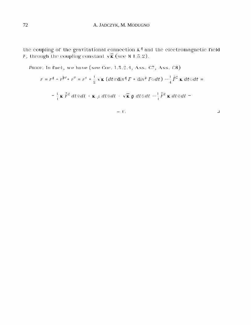
72 A. JADCZYK, M. MODUGNO
the coupling of the gravitational connection KŸ and the electromagnetic fieldF, through the coupling constant ¢Ãkkkk (see § I.3.2).
PROOF. In fact, we have (see Cor. I.3.2.4, Ass. C7, Ass. C8)
r = rŸ _ rŸe_ re = rŸ _ 12¢Ãkkkk (dtædivŸ F _ divŸ Fædt) - 1
4êF2 kkkk dtædt =
= 14kkkk êF2 dtædt _ kkkk µ dtædt _ ¢Ãkkkk ®®®® dtædt - 1
4êF2 kkkk dtædt =
= t. ò
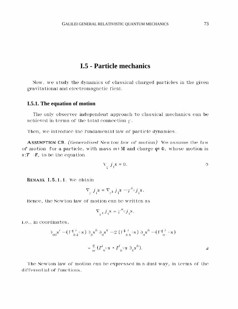
GALILEI GENERAL RELATIVISTIC QUANTUM MECHANICS 73
I.5 - Particle mechanics
Now, we study the dynamics of classical charged particles in the givengravitational and electromagnetic field.
I.5.1. The equation of motion
The only observer independent approach to classical mechanics can beachieved in terms of the total connection ˙.
Then, we introduce the fundamental law of particle dynamics.
AAAASSSSSSSSUUUUMMMMPPPPTTTTIIIIOOOONNNN CCCC9999. (Generalised Newton law of motion) We assume the lawof motion for a particle, with mass m$M and charge qqqq$Q, whose motion iss:TTTTéEEEE, to be the equation
ı j1s = 0. ò
RRRREEEEMMMMAAAARRRRKKKK IIII....5555....1111....1111. We obtain
ı j1s = ı
Ÿj1s - ˙e©j
1s.
Hence, the Newton law of motion can be written as
ıŸj1s = ˙e©j
1s,
i.e., in coordinates,
Ù00si - (ÍŸ
hik©s) Ù
0sh Ù
0sk - 2 (ÍŸ
0ih©s) Ù
0sh - (ÍŸ
0i©©s) =
= qm(Fi
0©s _ Fi
h©s Ù
0sh). ò
The Newton law of motion can be expressed in a dual way, in terms of thedifferential of functions.
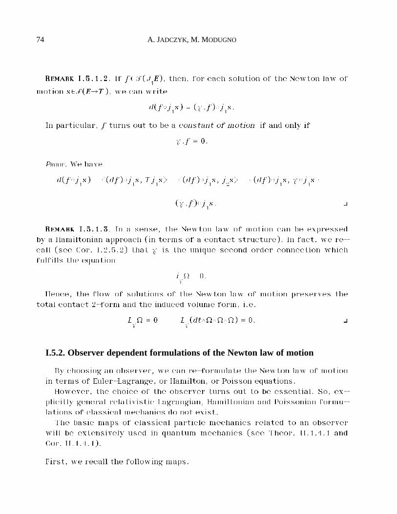
74 A. JADCZYK, M. MODUGNO
RRRREEEEMMMMAAAARRRRKKKK IIII....5555....1111....2222. If f$F(J1EEEE), then, for each solution of the Newton law of
motion s$S(EEEEéTTTT), we can write
d(f©j1s) = (˙.f)©j
1s.
In particular, f turns out to be a constant of motion if and only if
˙.f = 0.
PROOF. We have
d(f©j1s) = Ç(df)©j
1s, Tj
1s¶ = Ç(df)©j
1s, j
2s¶ = Ç(df)©j
1s, ˙©j
1s¶ =
= (˙.f)©j1s. ò
RRRREEEEMMMMAAAARRRRKKKK IIII....5555....1111....3333. In a sense, the Newton law of motion can be expressedby a Hamiltonian approach (in terms of a contact structure). In fact, we re-call (see Cor. I.2.5.2) that ˙ is the unique second order connection whichfulfills the equation
i˙Ò = 0.
Hence, the flow of solutions of the Newton law of motion preserves thetotal contact 2-form and the induced volume form, i.e.
L˙Ò = 0 L
˙(dt◊Ò◊Ò◊Ò) = 0. ò
I.5.2. Observer dependent formulations of the Newton law of motion
By choosing an observer, we can re-formulate the Newton law of motionin terms of Euler-Lagrange, or Hamilton, or Poisson equations.
However, the choice of the observer turns out to be essential. So, ex-plicitly general relativistic Lagrangian, Hamiltonian and Poissonian formu-lations of classical mechanics do not exist.
The basic maps of classical particle mechanics related to an observerwill be extensively used in quantum mechanics (see Theor. II.1.4.1 andCor. II.1.4.1).
First, we recall the following maps.
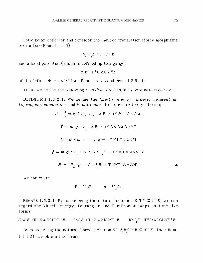
GALILEI GENERAL RELATIVISTIC QUANTUM MECHANICS 75
Let o be an observer and consider the induced translation fibred morphismsover EEEE (see Rem. I.1.1.3)
ıo:J1EEEEéT*ÆVEEEE
and a local potential (which is defined up to a gauge)
a:EEEEéT*ÆAÆT*EEEE
of the 2-form È ˆ 2 o*Ò (see Rem. I.2.2.2 and Prop. I.2.5.1).
Then, we define the following classical objects in a coordinate free way.
DDDDEEEEFFFFIIIINNNNIIIITTTTIIIIOOOONNNN IIII....5555....2222....1111. We define the kinetic energy, kinetic momentum,Lagrangian, momentum and Hamiltonian to be, respectively, the maps
GGGG ˆ 12m g©(ı
o, ı
o) : J
1EEEE é T*ÆT*ÆAÆM
êPPPP ˆ m g@©ıo: J
1EEEE é T*ÆAÆMÆV*EEEE
LLLL ˆ GGGG _ m dœa : J1EEEE é T*ÆT*ÆAÆM
êpppp ˆ m g@©ıo_ m dœa : J
1EEEE é T*ÆAÆMÆV*EEEE
HHHH ˆ Çıo, êpppp¶ - LLLL : J
1EEEE é T*ÆT*ÆAÆM. ¡
We can write
êPPPP = VEEEEGGGG êpppp = V
EEEELLLL.
RRRREEEEMMMMAAAARRRRKKKK IIII....5555....2222....1111. By considering the natural inclusion EEEE˚T* ç T*EEEE, we canregard the kinetic energy, Lagrangian and Hamiltonian maps as time-likeforms
GGGG:J1EEEEéT*ÆAÆMÆT*EEEE LLLL:J
1EEEEéT*ÆAÆMÆT*EEEE HHHH:J
1EEEEéT*ÆAÆMÆT*EEEE.
By considering the natural fibred inclusion ª*:J1EEEEEEEEV*EEEE ç T*EEEE (see Rem.
I.1.1.2), we obtain the forms
76 A. JADCZYK, M. MODUGNO
PPPP ˆ ª*œ êPPPP : J1EEEE é T*ÆAÆMÆT*EEEE pppp ˆ ª*œêpppp : J
1EEEE é T*ÆAÆMÆT*EEEE,
which will be said to be the kinetic momentum form and momentum form ,respectively. ò
Moreover, if u0$T_, then we set
G ˆ GGGG(u0,u0) : J
1EEEE é AÆMÆ· L ˆ LLLL(u
0,u0) : J
1EEEE é AÆMÆ·
H ˆ HHHH(u0,u0) : J
1EEEE é AÆMÆ·
êP ˆ êPPPP(u0) : J
1EEEE é AÆMÆV*EEEE êp ˆ êpppp(u
0) : J
1EEEE é AÆMÆV*EEEE
P ˆ PPPP(u0) : J
1EEEE é AÆMÆT*EEEE p ˆ pppp(u
0) : J
1EEEE é AÆMÆT*EEEE.
RRRREEEEMMMMAAAARRRRKKKK IIII....5555....2222....2222. With reference to a space-time chart adapted to theframe of reference (u
0, o), we have the following coordinate expressions
G = 12m g
ijy0i y
0j L = 1
2m g
ijy0i y
0j _ m (a
iy0i _ a
0)
H = 12m g
ijy0i y
0j - m a
0
êP = m gijy0j êdi êp = (m g
ijy0j _ m a
i) êdi
P = - m gijy0i y
0j d0 _ m g
ijy0j di p = - m g
ijy0i y
0j d0 _ (m g
ijy0j _ m a
i) di.
RRRREEEEMMMMAAAARRRRKKKK IIII....5555....2222....3333. Let o and o' be two observers and set
v ˆ o' - o : EEEE é T*ÆVEEEE.
Then, we obtain the following relation between the respective kineticforms
GGGG' = GGGG _ 12m g©(v,v) - m ı
oœv@ PPPP' = PPPP - m ª*œv@,
hence (see Remark I.1.1.3)
GALILEI GENERAL RELATIVISTIC QUANTUM MECHANICS 77
GGGG' _ PPPP' = GGGG _ PPPP _ 12m g©(v,v) - m ~
0*œv@,
where
v@ ˆ g@©v : EEEEéT*ÆAÆV*EEEE.
PROOF. It follows from
ıo'= ı
o- v ı
o_ ª* = ~
o. ò
RRRREEEEMMMMAAAARRRRKKKK IIII....5555....2222....4444. We can achieve a Hamiltonian formulation of the Newtonlaw of motion in three different ways, by considering the symplectic struc-tures naturally induced by the total contact 2-form Ò on the even dimen-sional vector bundles
VJ1EEEEéJ
1EEEE VVEEEEéVEEEE VV*EEEEéV*EEEE
and the observer dependent Hamiltonian and momentum functions.Moreover, the Newton law of motion, in the version quoted in Rem. I.5.1.2,
can be expressed in terms of the Poisson bracket (see, later, Prop. II.3.2.1)between the function f$F(J
1EEEE) and the observer dependent Hamiltonian
function.Furthermore, the Newton law of motion turns out to be the Euler-Lagrange
equation associated with the observer dependent Lagrangian function.We omit here the details. ò
78 A. JADCZYK, M. MODUGNO
I.6 - Special relativistic case
Under reasonable hypothesis, there exist distinguished metrical space-time connections, which yield an affine structure on space-time. In such acase, we avail of this structure to simplify several formulas; in particular,we prove that the Einstein equation turns out to be just the Newton law ofgravitation.
In the special case when the energy tensor vanishes, possibly the samegravitational connection yields an affine structure on space-time. Such adistinguished solution of the field equations is referred to as special rela-tivistic and constitutes the background for the standard classical New-tonian mechanics.
I.6.1. Affine structure of space-time
Let us start with preliminary observations on a possible background con-nection inducing an affine structure on space-time.
RRRREEEEMMMMAAAARRRRKKKK IIII....6666....1111....1111. Let A be an affine space associated with the vectorspace ÃA and the translation map f:A˚ÃAéA.
Then, the affine structure yields a linear connection on A
~K»: TTA = (A˚ÃA)˚(ÃA˚ÃA) é VTA = (A˚ÃA)˚(0˚ÃA) : (a,u;v,w) ´ (a,u;0,w),
which is geodesically complete and whose curvature vanishes.Conversely, the above connection K» characterises naturally the affine
structure (ÃA, f) on A in a unique way. ò
DDDDEEEEFFFFIIIINNNNIIIITTTTIIIIOOOONNNN IIII....6666....1111....1111. A background connection is defined to be a space-time connection K», such that
- K» is metrical (see § I.2.3), i.e. ı»ãg = 0;- K» induces an affine structure on the space-time manifold EEEE, such that
the time function t is an affine map. ¡
LLLLEEEEMMMMMMMMAAAA IIII....6666....1111....1111. Let K» be a background connection.Then, t:EEEEéTTTT turns out to be an affine bundle associated with a trivial
GALILEI GENERAL RELATIVISTIC QUANTUM MECHANICS 79
vector bundle
ãt : ÃEEEE = TTTT˚SSSS é TTTT,
where SSSS is a three dimensional vector space. Thus, t:EEEEéTTTT turns out to be aprincipal bundle.
Moreover, the vertical metric can be regarded as a constant element
g $ AÆSSSS*ÆSSSS*.
PROOF. Set
SSSS ˆ ker Dt ç DE,
where DE denotes the vector space associated with the affine space E.Then, for each †$TTTT, we obtain
D(t-1(†)) = SSSS,
in virtue of the fact that t is affine. ò
RRRREEEEMMMMAAAARRRRKKKK IIII....6666....1111....2222. Not all space-times t:EEEEéTTTT admit background connectionsK».
If the space-time t:EEEEéTTTT admits a background connection K», then we caneasily see that it admits many background connections. ò
RRRREEEEMMMMAAAARRRRKKKK IIII....6666....1111....3333. Let K» be a background connection. If o and o' are globalobservers such that
ıK»o = 0 = ı
K»o',
then we have
o' = o _ v v $ T*ÆSSSS. ò
RRRREEEEMMMMAAAARRRRKKKK IIII....6666....1111....4444. Let K» be a background connection. Then, each global
space-time chart (x0,yi) adapted to the induced affine structure of space-time yields
K»¬iµ= 0 g
ij$ A.
Of course, the observer o associated with such a chart is of the abovetype. ò
80 A. JADCZYK, M. MODUGNO
I.6.2. Newtonian connections and the Newton law of gravitation
Next, we consider the interesting case of a background connection whichis “tangent” to the gravitational connections on the fibres of space-time.
By considering such a connection, we can write the first and secondgravitational equations in an interesting way.
If the source of the gravitational connection KŸ is an incoherent fluid, thenthe gravitational Einstein equation implies that the vertical gravitational
connection êKŸ is flat (see Prop. I.4.5.2). Then, under further reasonable hy-
pothesis, êKŸ may induce an affine structure on the fibres of space-time. Ofcourse, if the mass density of the source does not vanish, KŸ cannot inducean affine structure on the whole space-time. However, under further reason-
able hypothesis, êKŸ may be extended to a background connection K» (in a nonunique way). So, we introduce the following notion.
DDDDEEEEFFFFIIIINNNNIIIITTTTIIIIOOOONNNN IIII....6666....2222....1111. A Newtonian connection is defined to be a space-time connection K» which fulfills the following properties:
i) the restrictions of K» and KŸ to the vertical subspace coincide
K»¡VEEEE
= KŸ¡VEEEE
: VEEEE é T*EEEEÆTEEEETVEEEE;;;;
ii) K» induces an affine structure on the space-time manifold EEEE, such thatthe time function t is an affine map. ¡
If K» is a Newtonian connection, then a Newtonian observer is defined tobe a global observer o such that ı
K»o = 0 and a Newtonian chart is defined to
be a global space-time chart (x0,yi) adapted to the induced affine structureof space-time.
Now on, in this section, we assume that a Newtonian connection K» existand we refer to such a connection K» and to Newtonian observers and charts.
Accordingly, some formulas of the classical field theory and particle me-chanics assume a simplified expression.
RRRREEEEMMMMAAAARRRRKKKK IIII....6666....2222....1111. Condition i) implies
êK» = êKŸ.
But we stress that condition i) is stronger than the above equality. ò
GALILEI GENERAL RELATIVISTIC QUANTUM MECHANICS 81
LLLLEEEEMMMMMMMMAAAA IIII....6666....2222....1111. The connection K» is metrical, hence it is a backgroundconnection.
PROOF. Condition i) and the first gravitational equation (see Prop. I.4.4.2)yield
ı»ãg = ıŸãg = 0. ò
LLLLEEEEMMMMMMMMAAAA IIII....6666....2222....2222. Condition i) reads in coordinates as
KŸ¬ij= 0. ò
LLLLEEEEMMMMMMMMAAAA IIII....6666....2222....3333. The gravitational connection can be uniquely written as
KŸ = K» _ dtædtæNŸ
where N is a section
NŸ:EEEEé(T*ÆT*)ÆVEEEE
whose coordinate expression is of the type
NŸ = NŸ0i0u0æu0æÙ
i, NŸ
0i0$F(EEEE).ò
We say that NŸ is the Newton vector field associated with the Newtonianconnection K».
Let us discuss at which extent the Newtonian connection is uniquely de-termined by the gravitational connection (provided at least one Newtonianconnection exists).
PPPPRRRROOOOPPPPOOOOSSSSIIIITTTTIIIIOOOONNNN IIII....6666....2222....1111. Let us suppose that K» and K»' be two Newtonianconnections.
Then, the two affine structures induced by K» and K»' on the space-timemanifold EEEE yield the same affine structure on the bundle t:EEEEéTTTT. Hence, weobtain the same vector bundle
ãt : ÃEEEE = TTTT˚SSSS é TTTT,
with respect to the two Newtonian connections.Moreover, the Newtonian vector fields associated with K» and K»' differ by
82 A. JADCZYK, M. MODUGNO
a time-dependent vector field:
(*) NŸ' - NŸ : TTTT é (T*ÆT*)ÆSSSS.
Furthermore, let o and o' be two Newtonian observers with respect to K»and K»', respectively. Then, the two observers perform mutually a rigid
translation13:
(**) o' - o : TTTT é T*ÆSSSS.
PROOF. The affine structures induced on the fibres of space-time by K» andK»' coincide because
êK» = êKŸ = êK»'.
In other words, K» and K»' induce on the space-time fibred manifold thesame structure of affine bundle, associated with the vector bundle
VVVVéTTTT.
Hence, K» and K»' induce the same vertical parallelisation
VEEEE = EEEEBBBBVVVV.
Moreover, we have
ıŸ(o' - o) = ıŸo' - ıŸo = (ı»'o' - dtædtæNŸ') - (ı»o - dtædtæNŸ) =
= dtædtæ(NŸ - NŸ'),
which yields
(i) ıŸ(o' - o) = dtædtæ(NŸ - NŸ').
The vertical restriction of (i) gives
êıŸ(o' - o) = 0,
i.e. o' - o can be regarded as a section
(**) o' - o : TTTT é T*ÆVVVV.
13 As usual, the difference o' - o is taken with respect to the affinestructure of the bundle J
1EEEEéEEEE.
GALILEI GENERAL RELATIVISTIC QUANTUM MECHANICS 83
Furthermore, formula (*) implies that ıŸ(o' - o) can be regarded as a sec-tion
(ii) ıŸ(o' - o) : TTTT é T*ÆT*ÆVVVV.
Then, formulas (i) and (ii) yield (*).Additionally, formula (**) implies that o and o' yield the same linear split-
ting over TTTT
VVVVéTTTT˚SSSS. ò
Next, let us show that the first and second gravitational equation implythat N fulfills the Newton law of gravitation.
RRRREEEEMMMMAAAARRRRKKKK IIII....6666....2222....2222. The 2-form ÒŸ becomes
ÒŸ = Ò» - Çdt,NŸ¶◊ª.
Let o be a Newtonian observer. Then the 2-form ÈŸ becomes
ÈŸ = 2 NŸ@◊dt. ò
PPPPRRRROOOOPPPPOOOOSSSSIIIITTTTIIIIOOOONNNN IIII....6666....2222....2222. The first gravitational field equation reduces to
êdNŸ@ = 0.
PROOF. Let o be a Newtonian observer. Then, we obtain
êKŸ = êK» = º êÁŸ = êÁ» = 0 êÈ» = 0.
Hence, the first field equation (see Theorem I.4.3.1) reduces to êdNŸ@ = 0. ò
CCCCOOOORRRROOOOLLLLLLLLAAAARRRRYYYY IIII....6666....2222....1111. The first gravitational field equation reduces to
NŸ = êgrad U,
where U is a map
UŸ:EEEEéT*ÆT*ÆA. ò
LLLLEEEEMMMMMMMMAAAA IIII....6666....2222....4444. The Ricci tensor of the gravitational connection turns outto be
84 A. JADCZYK, M. MODUGNO
rŸ = êdivŸ NŸ dtædt : EEEE é T*EEEEÆEEEET*EEEE. ò
Next, let us assume that the source of the gravitational connection KŸ isan incoherent fluid with density mass µ, as in § I.4.5. This hypothesis doesnot conflict with the above lemma, as both rŸ and tŸ turn out to be time-liketensors.
Then, we can re-interpret the second gravitational field equation as fol-lows.
TTTTHHHHEEEEOOOORRRREEEEMMMM IIII....6666....2222....1111. The second gravitational field equation reduces to
êdivŸ NŸ = kkkkæµ,
i.e. to
êË» U = kkkkæµ. ò
RRRREEEEMMMMAAAARRRRKKKK IIII....6666....2222....2222. Let o be a Newtonian observer. The potential of ÈŸ be-comes
aŸ = Uædt. ò
We can express the curvature through the gravitational potential.
RRRREEEEMMMMAAAARRRRKKKK IIII....6666....2222....3333. Let us regard dtædtæNŸ as a vertical valued 1-form onthe vector bundle TEEEEéEEEE
dtædtæNŸ:TEEEEéT*EEEEÆEEEEVEEEE.
Then, the gravitational curvature turns out to be the covariant exteriordifferential (see § III.5) of NŸ, with respect to the background connectionK»,
RŸ = dK»(dtædtæNŸ),
with coordinate expression
RŸ = u0æu
0ægih Ù
hjU dj◊d0æÙ
iæd0.
PROOF. We have (see Rem. I.1.1.3)
GALILEI GENERAL RELATIVISTIC QUANTUM MECHANICS 85
RŸ = 12[KŸ, KŸ] = 1
2[K» _ dtædtæNŸ, K» _ dtædtæNŸ] = [K», dtædtæNŸ] ˆ
ˆ dK»(dtædtæNŸ) . ò
Finally, we study the law of motion of a classical test particle in the andshow that it reduces exactly to the classical Newton law of gravitation.
LLLLEEEEMMMMMMMMAAAA IIII....6666....2222....5555. The gravitational second order connection can be writtenas
˙Ÿ = ˙» _ NŸ,
where ˙» is the second order connection associated with Í». ò
PPPPRRRROOOOPPPPOOOOSSSSIIIITTTTIIIIOOOONNNN IIII....6666....2222....3333. The Newton law of motion reads as
ı»s = NŸ©js. ò
Therefore, NŸ can be interpreted as the gravitational force with respect tothe background connection K».
RRRREEEEMMMMAAAARRRRKKKK IIII....6666....2222....4444. Two different Newtonian connections K» and K»' yieldtwo different accelerations and gravitational forces
ı»s ı
»'s NŸ©js NŸ'©js. ò
RRRREEEEMMMMAAAARRRRKKKK IIII....6666....2222....5555. Neither the two fields equations, nor the law of motionyield any distinguished choice among Newtonian connections admitted by KŸ(if they exist). ò
I.6.3. The special relativistic space-time
Eventually, we consider the case when the source of the gravitationalfield vanishes. In this case, the gravitational connection is Ricci flat;hence it is possibly flat and, under reasonable hypothesis, the gravitationalconnection itself is a Newtonian connection. So, in this case, we have adistinguished choice of the Newtonian background connection.
Therefore, we are led to introduce the following notion.
86 A. JADCZYK, M. MODUGNO
DDDDEEEEFFFFIIIINNNNIIIITTTTIIIIOOOONNNN IIII....6666....3333....1111. A space-time is said to be special if the gravitationalconnection KŸ induces an affine structure on the space-time manifold EEEE, suchthat the time function t is an affine map. ¡
Of course, if the space-time is special, then we can apply all above resultswith the identifications
K» = KŸ NŸ = 0.
This case will be referred to as the special relativistic Galilei case. Thecorresponding field theory and mechanics are just the standard classicaltheories.
GALILEI GENERAL RELATIVISTIC QUANTUM MECHANICS 87
I.7 - Classical two-body mechanics
So far, space-time has been regarded as the manifold of possible events“touched” by a classical particle. Moreover, the source of gravitational andelectromagnetic fields has been a given external incoherent charged fluid(as an example). Furthermore, we have described the mechanics of a clas-sical particle.
Now, we modify slightly our model in order to describe a closed systemconstituted by n classical particles interacting through the gravitationaland electromagnetic fields. Thus, we no longer consider an external sourceof the fields, but the source is constituted by the particles themselves.Then, we are led to consider the fibred product over time of n identicalcopies of the “pattern” space-time as the framework of the system; eachcomponent is referred to one of the n particles. In order to describe thesingularities corresponding to the possible collisions, we could describethe fields in terms of distributions. However, we follow a simpler way: wejust cut the multi-events corresponding to possible collisions and considersmooth fields. It is a striking fact that the fields and the mechanics ofparticles can be formulated in terms of this multi-space-time in stronganalogy with the case of a single particle. Actually, in the one particletheory, the dimension 3 of the space-time fibre has never played an es-sential role. So, the basic change from the case n = 1 to the case n > 1consists in the increase of the dimension of the fibre of space-time (alongwith the addition of n projections on the components).
This scheme can be developed for any n ≥ 1. However, we do it explicitlyonly for the case n = 2. The reader can generalise it without any difficulty.
We do not find the most general solution of field equations, but we justexhibit the simplest solution whose symmetries and boundary conditionsare physically sensible. Then, the classical dynamics follows easily. Thissolution is nothing but a Galilei general relativistic formulation of the wellknown standard classical two body problem. We stress that the fieldequations and solutions can be formulated independently of the explicitmotion of the particles.
Many concepts and results of this chapter are quite simple and standard.
88 A. JADCZYK, M. MODUGNO
However, it is necessary to spend some words for fixing the notation andshowing how standard notions arise very well in our general formalism.
I.7.1. Two body space-time and equations
We start by introducing the multi-space-time associated with two clas-sical particles. We consider the associated basic multi-objects such as themetric, gravitational and electromagnetic fields and we write the multi-field equations.
We label the objects related to the two particles by the indices 1 and 2,respectively.
AAAASSSSSSSSUUUUMMMMPPPPTTTTIIIIOOOONNNN CCCCTTTTBBBB1111. We assume a space-time fibred manifold
t:EEEEéTTTT
as in Assumption C1, which will be referred to as the pattern space-time. ò
More generally, the adjective pattern will be used for all objects associ-ated with the pattern space-time.
Then, we define the multi-space-time to be the fibred manifold
ttttt : EEEEE ˆ (EEEE1)TTTT(EEEE
2) é TTTT
where EEEE1and EEEE
2are two identical copies of the pattern space-time EEEE:
EEEE1+ EEEE + EEEE
2.
We denote the projections on the two components by
p1:EEEEEéEEEE
1p2:EEEEEéEEEE
2.
Of course, we can write
TEEEEE = (TEEEE1)TTTTT(TEEEE
2) VEEEEE = (VEEEE
1)TTTT(VEEEE
2) J
1EEEEE = (J
1EEEE1)TTTT(J1EEEE2).
Moreover, we consider the reduced multi-space-time obtained by sub-tracting the diagonal from the multi-space-time:
ttttt' : EEEEE' ˆ (y1,y
2) $ EEEEE ¡ y
1= y
2 é TTTT.
GALILEI GENERAL RELATIVISTIC QUANTUM MECHANICS 89
Then, we can define multi-objects related to multi-space-time analogouslyto the one body theory. Let us analyse a few concepts as an example.
A multi-motion is defined to be a section
sssss:TTTTàEEEEE
and its velocity is defined to be its first jet prolongation
j1sssss:TTTTéJ
1EEEEE.
Of course, we can write
sssss = (s1,s2) ˆ (sssss©pr
1,sssss©pr
2) j
1sssss = (j
1s1,j1s2) ˆ ⁄j
1(sssss©pr
1),j
1(sssss©pr
2)^,
where
s1:TTTTéEEEE
1s2:TTTTéEEEE
2j1s1:TTTTéJ
1EEEE1
j1s2:TTTTéJ
1EEEE2.
A multi-observer is defined to be a section
ooooo:EEEEEéJ1EEEEE.
Of course, we can write
ooooo = (o1,o2) ˆ (ooooo©J
1pr
1,ooooo©J
1pr
2),
where
o1:EEEEEéJ
1EEEE1
o2:EEEEEéJ
1EEEE2,
need not to be pattern observers in the standard sense because they may de-pend on the two-body events. In particular, let
o:EEEEéJ1EEEE
be a pattern observer and let o1and o
2be two identical copies of o on EEEE
1and
EEEE2, respectively; then, o yields the multi-observer
ooooo ˆ (o1,o2).
A pattern space-time chart (x0,yi) yields the multi-space-time chart
90 A. JADCZYK, M. MODUGNO
(x0, y1i, y
2i) ˆ (x0, yi©pr
1, yi©pr
1).
Next, we pursue by assuming further structures on the multi-space-timeanalogously to the one body case.
AAAASSSSSSSSUUUUMMMMPPPPTTTTIIIIOOOONNNN TTTTBBBB2222. We assume the reduced multi-space-time to beequipped with a multi-metric
ggggg:EEEEE'éAÆ(V*EEEEEÆEEEEEV*EEEEE),
a multi-gravitational connection
KKKKKŸ:TEEEEE'éT*EEEEE'ÆEEEEE ''''TTEEEEE'
and a multi-electromagnetic field
FFFFF:EEEEE'éBÆL2T*EEEEE'. ò
Analogously to the one body case, the above fields yield several objects,which fulfill several relations. In particular, we obtain the multi-gravita-tional connection (see Prop. I.2.1.1)
ÍÍÍÍÍŸ:J1EEEEE'éT*EEEEE' Æ
J1EEEEE''''TJ
1EEEEE',
the multi-second order gravitational connection (see Prop. I.2.5.1)
˙Ÿ:J1EEEEE'éT* Æ
J1EEEEE''''TJ
1EEEEE',
the multi-gravitational contact 2-form (see Prop. I.2.5.2)
ÒÒÒÒÒŸ:J1EEEEE'é(T*ÆA)ÆL
2T*J
1EEEEE'
the multi-gravitational curvature tensor (see Rem. I.2.1.4)
RRRRRŸ:EEEEE'é L2T*EEEEE'Æ
EEEEE''''V*EEEEE'.
and the multi-gravitational Ricci tensor (see Rem. I.2.1.4)
rrrrrŸ:EEEEE'éT*EEEEE'ÆEEEEE''''T*EEEEE'.
GALILEI GENERAL RELATIVISTIC QUANTUM MECHANICS 91
AAAASSSSSSSSUUUUMMMMPPPPTTTTIIIIOOOONNNN TTTTBBBB3333. We assume two masses and charges
m1, m
2$ M qqqq
1, qqqq
2$ Q. ò
We set
µ1ˆ
m1m
m ˆ m1_ m
2µ2ˆ
m2m
¯1ˆ
qqqq1qqqq
qqqq ˆ qqqq1_ qqqq
2¯2ˆ
qqqq2qqqq.
Then, we obtain the multi-total objects by coupling the gravitational andelectromagnetic fields (see § I.3.2), analogously to the case of one particle,both with reference to the above mass m$M and charge qqqq$Q and to thesquare root of the universal gravitational constant kkkk.
In particular, we have the following total objects (with respect to bothcouplings)
ÍÍÍÍÍ = ÍÍÍÍÍŸ _ ÍÍÍÍÍe ˙ = ˙Ÿ _ ˙e ÒÒÒÒÒ = ÒÒÒÒÒŸ _ ÒÒÒÒÒe.
Moreover, we obtain the following splittings
RRRRR = RRRRRŸ _ RRRRRŸe _ RRRRRe rrrrr = rrrrrŸ _ rrrrrŸe _ rrrrre.
The one body field theory suggests the following field equations.
AAAASSSSSSSSUUUUMMMMPPPPTTTTIIIIOOOONNNN TTTTBBBB4444. We assume the metric, gravitational and electromag-netic field to fulfill the following field equations on the reduced multi-space-time
d ÒÒÒÒÒŸ = 0 dFFFFF = 0
rrrrrŸ = 0 divŸFFFFF = 0 ò
The one body mechanics suggests the following dynamical equation.
AAAASSSSSSSSUUUUMMMMPPPPTTTTIIIIOOOONNNN TTTTBBBB5555. (Generalised Newton law of motion) We assume thelaw of motion for two particles, with masses m
1, m
2$M and charges qqqq
1,
92 A. JADCZYK, M. MODUGNO
qqqq2$Q, whose multi-motion is sssss:TTTTéEEEEE, to be the equation
ı˙j1sssss = 0. ò
Later, in the two body quantum mechanics (see § II.7.2), we shall be in-volved with the following classical objects.
Let us consider a multi-observer ooooo and the associated map
ıooooo:J1EEEEEéT*ÆVEEEEE.
Then, we define the multi-kinetic energy and multi-kinetic momentum tobe the maps (see Def. I.5.2.1)
GGGGG ˆ 12m ggggg©(ı
ooooo, ı
ooooo) : J
1EEEEE é T*ÆT*ÆAÆM
êPPPPP ˆ m ggggg@©ıooooo: J
1EEEEE é T*ÆAÆMÆV*EEEEE.
Moreover, we obtain the kinetic energy form and kinetic momentum form(see Rem. I.5.2.1)
GGGGG:J1EEEEEéT*ÆAÆMÆT*EEEEE
PPPPP ˆ ªªªªª*œ êPPPPP : J1EEEEE é T*ÆAÆMÆT*EEEEE.
I.7.2. The standard two-body solution
Next, we exhibit a distinguished solution of the field equations whosesymmetries and boundary values are physically appropriate.
The background space-time structure
First, we introduce a multi-metric and a background affine structure ofthe multi-space-time in the following way.
We consider a vertical metric (see § I.1.2)
g:EEEEéAÆ(V*EEEEÆEEEEV*EEEE)
and a background connection (see Def. I.6.1.1)
GALILEI GENERAL RELATIVISTIC QUANTUM MECHANICS 93
K»:TEEEEéT*EEEEÆEEEETTEEEE
on the pattern space-time.Then, we denote by g
1and g
2two identical copies of g on EEEE
1and EEEE
2, re-
spectively, and consider the multi-metric
ggggg:EEEEEéAÆ(V*EEEEEÆEEEEEV*EEEEE)
given by
ggggg : VEEEEEÆEEEEEVEEEEE é A : (X,Y) ´ µ
1g1(X
1,Y1) _ µ
2g2(X
2,Y2).
Analogously, we denote by K»1and K»
2two identical copies of K» on EEEE
1and
EEEE2, respectively, and consider the multi-background connection
KKKKK» ˆ K»1˚K»
2: TEEEEEéT*EEEEEÆ
EEEEETTEEEEE.
Hence, the background affine structure on the multi-space-time yields thesplittings (see Lemma I.6.1.1)
ÃEEEEE = TTTT˚SSSSS VEEEEE = EEEEE˚SSSSS,
where SSSSS is the 6-dimensional vector space
SSSSS = SSSS1˚SSSS
2,
where SSSS1and SSSS
2denote two identical copies of SSSS related to EEEE
1and EEEE
2, re-
spectively.We consider also the reduced subset
SSSS' ˆ SSSS - 0.
Moreover, the multi-metric turns out to be an element
ggggg $ AÆ⁄(SSSS1*ÆSSSS
1*)˚(SSSS
2*ÆSSSS
2*)^.
Before pursuing with the construction of the standard solution of the fieldequations, we analyse some important consequences of the above structureson the multi-space-time.
94 A. JADCZYK, M. MODUGNO
We define the space of the centre of mass to be the diagonal fibred sub-manifold over TTTT
EEEEEcˆ (e
1,e2) $ EEEEE ¡ e
1= e
2 ç EEEEE é TTTT
and the centre of mass projection to be the fibred morphism over TTTT
prc: EEEEE é EEEEE
c: eeeee + (e
1,e2) ´ eeeee
c+ (e
c,ec),
where ec$ EEEE is the unique element such that
t(e1) = t(e
c) = t(e
2) µ
1(e
1- e
c) _ µ
2(e
2- e
c) = 0.
Moreover, we define the relative space to be the vector subspace
SSSSSsˆ (X
1,X
2) $ SSSSS ¡ µ
1X1_ µ
2X2= 0 ç SSSSS
and the c-relative projection to be the map
prs: EEEEE é SSSSS
s: eeeee + (e
1,e2) ´ sssss + (ssss
1,ssss2) ˆ (e
1- e
c, e
2- e
c).
Furthermore, we define the relative projections to be the map14
prr: EEEEEéSSSSS : eeeee + (e
1,e2) ´ (rrrr
1,rrrr2) ˆ (e
1- e
2, e
2- e
1).
We set also
® : SSSS é A1/2Æ· : v ´ ˜v˜ ˆ ÊÕÕg(v,v)
r ˆ ®©rrrr1= ®©rrrr
2: EEEEE é A
1/2Æ·
s ˆ ˜sssss˜ ˆ ÊÕÕôggggg(sssss,sssss) .
Hence, we can write
rrrr1= 1µ2ssss1
r2 = 1µ1µ2s2 rrrr
2= 1µ1ssss2.
Therefore, besides the natural fibred splitting over TTTT
14 Of course, these maps should not be confused with the Ricci tensor.
GALILEI GENERAL RELATIVISTIC QUANTUM MECHANICS 95
(pr1,pr
2) : EEEEE é EEEE
1 TTTTEEEE2: eeeee ´ (e
1, e
2),
we obtain the further splittings induced by the affine background structure
(prc,pr
s) : EEEEE é EEEEE
c˚SSSSS
s: eeeee ´ ⁄e
c, (ssss
1,ssss2)^ ˆ (e
c, (e
1- e
c, e
2- e
c)^
(prc,pr
r1) : EEEEE é EEEEE
c˚SSSS : eeeee ´ (e
c, rrrr
1) ˆ (e
c, e
1- e
2)
(prc,pr
r2) : EEEEE é EEEEE
c˚SSSS : eeeee ´ (e
c, rrrr
2) ˆ (e
c, e
2- e
1).
The above splitting is naturally prolonged by the tangent and jet functors,hence it yields analogous splittings of structures and equations.
If o is a pattern Newtonian observer and (x0,yi) an adapted Cartesianchart, then we obtain the two distinguished multi-charts
(x0, y1i, y
1i) ˆ (x0, yi©pr
1, yi©pr
2) (x0, y
ci, y
ri) ˆ (x0, yi©pr
c, y
2i - y
1i).
The gravitational and electromagnetic fields
Next, we exhibit the multi-gravitational connection.We consider the map
UŸ ˆ -kkkk
m
m1m2
®: SSSS' é T*ÆT*ÆAÆM,
which yields
UUUUUŸ ˆ UŸ©rrrr1= UŸ©rrrr
2: EEEEE'éT*ÆT*ÆA.
Then, we obtain the section
NNNNNŸ ˆ êgrad UUUUUŸ : EEEEE'é(T*ÆT*)ÆVEEEEE,
which can be expressed as
NNNNNŸ = (NŸ1,NŸ
2) = -
kkkk
m
m1m2
r3( 1µ1rrrr1, 1µ2rrrr2).
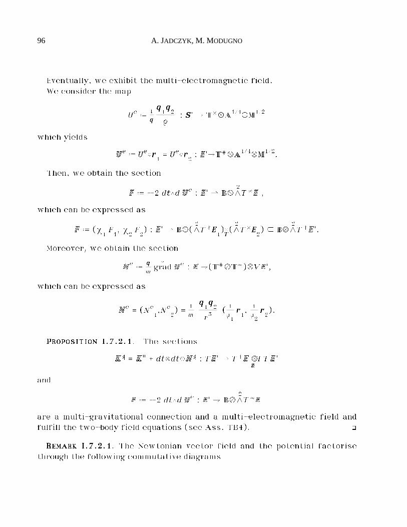
96 A. JADCZYK, M. MODUGNO
Eventually, we exhibit the multi-electromagnetic field.We consider the map
Ue ˆ 1qqqq
qqqq1qqqq2
®: SSSS' é T*ÆA1/4ÆM1/2
which yields
UUUUUe ˆ Ue©rrrr1= Ue©rrrr
2: EEEEE'éT*ÆA1/4ÆM1/2.
Then, we obtain the section
FFFFF ˆ - 2 dt◊d UUUUUe : EEEEE' é BÆL2T*EEEEE',
which can be expressed as
FFFFF ˆ (¯1F1, ¯
2F2) : EEEEE' é BÆ(L
2T*EEEE
1)TTTT(L2T*EEEE
2) ç BÆL
2T*EEEEE'.
Moreover, we obtain the section
NNNNNe ˆ qqqqm
êgrad UUUUUe : EEEEE'é(T*ÆT*)ÆVEEEEE',
which can be expressed as
NNNNNe = (Ne1,Ne
2) = 1
m
qqqq1qqqq2
r3( 1µ1rrrr1, 1µ2rrrr2).
PPPPRRRROOOOPPPPOOOOSSSSIIIITTTTIIIIOOOONNNN IIII....7777....2222....1111. The sections
KKKKKŸ = KKKKK» _ dtædtæNNNNNŸ : TEEEEE' é T*EEEEE'ÆEEEEE'TTEEEEE'
and
FFFFF ˆ - 2 dt◊d UUUUUe : EEEEE' é BÆL2T*EEEEE'
are a multi-gravitational connection and a multi-electromagnetic field andfulfill the two-body field equations (see Ass. TB4). ò
RRRREEEEMMMMAAAARRRRKKKK IIII....7777....2222....1111. The Newtonian vector field and the potential factorisethrough the following commutative diagrams
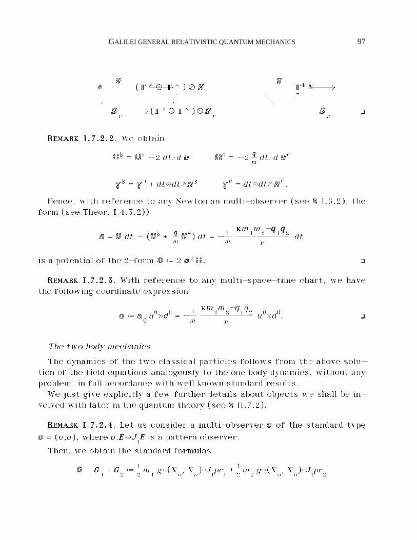
GALILEI GENERAL RELATIVISTIC QUANTUM MECHANICS 97
EEEEE äNNNNN
(T * Æ T * ) Æ SSSSS EEEEEäUUUUU
T*
ï À ö ÖSSSSSrä(T*ÆT*)ÆSSSSS
rSSSSSr
ò
RRRREEEEMMMMAAAARRRRKKKK IIII....7777....2222....2222. We obtain
ÒÒÒÒÒŸ = ÒÒÒÒÒ» - 2 dt◊d UUUUU ÒÒÒÒÒe = - 2 qqqqmdt◊d UUUUUe
˙Ÿ = ˙» _ dtædtæNNNNNŸ ˙e = dtædtæNNNNNe.
Hence, with reference to any Newtonian multi-observer (see § I.6.2), theform (see Theor. I.4.3.2))
aaaaa = UUUUU dt ˆ (UUUUUŸ _ qqqqmUUUUUe) dt = - 1
m
kkkkm1m2-qqqq
1qqqq2
rdt
is a potential of the 2-form ÈÈÈÈÈ ˆ 2 ooooo*ÒÒÒÒÒ. ò
RRRREEEEMMMMAAAARRRRKKKK IIII....7777....2222....3333. With reference to any multi-space-time chart, we havethe following coordinate expression
aaaaa ˆ aaaaa0u0æd0 = - 1
m
km1m2-q
1q2
ru0æd0. ò
The two body mechanics
The dynamics of the two classical particles follows from the above solu-tion of the field equations analogously to the one body dynamics, without anyproblem, in full accordance with well known standard results.
We just give explicitly a few further details about objects we shall be in-volved with later in the quantum theory (see § II.7.2).
RRRREEEEMMMMAAAARRRRKKKK IIII....7777....2222....4444. Let us consider a multi-observer ooooo of the standard type
ooooo = (o,o), where o:EEEEéJ1EEEE is a pattern observer.
Then, we obtain the standard formulas
GGGGG = GGGG1_ GGGG
2ˆ 1
2m1g©(ı
o, ı
o)©J
1pr
1_ 1
2m2g©(ı
o, ı
o)©J
1pr
2
98 A. JADCZYK, M. MODUGNO
= GGGGc_ GGGG
rˆ 1
2m g©(ı
o, ı
o)©J
1pr
c_ 1
2m µ
1µ2g©(ı
o, ı
o)©J
1pr
r
êPPPPP = êPPPP1_ êPPPP
2ˆ (m
1g@©ı
o)©J
1pr
1_ (m
2g@©ı
o)©J
1pr
2
= êPPPPc_ êPPPP
rˆ (m g@©ı
o)©J
1pr
c_ (m µ
1µ2g@©ı
o)©J
1pr
r
PPPPP = PPPP1_ PPPP
2ˆ ª*œ êPPPP
1_ ª*œ êPPPP
2
= PPPPc_ PPPP
rˆ ª*œ êPPPP
c_ ª*œ êPPPP
r.
With reference to a Cartesian chart (x0,yi) adapted to o, we obtain thefollowing coordinate expressions
GGGGG = 12∂ij(m
1y1i0y10j _ m
2y2i0y20j)
= 12∂ijm (y
ci0yc0j _ µ
1µ2yri0yr0j)
PPPPP = - ∂ij⁄(m
1y10i y
10j _ m
2y20i y
20j) d0 _ (m
1y10j d
1i _ m
2y20j d
2i)^
= - ∂ijm ⁄(y
ci0yc0j _ µ
1µ2yri0yr0j) d0 _ (y
c0j d
ci _ µ
1µ2yr0j d
ri)^. ò
We conclude this chapter with the observation that, in most respects, thesystem of two particles with masses (m
1,m
2) and charges (qqqq
1,qqqq
2) can be
treated just as a system consisting of one particle with mass m and charge qqqqmoving in the multi-space-time.
GALILEI GENERAL RELATIVISTIC QUANTUM MECHANICS 99
II - THE QUANTUM THEORY
The second part of the paper is devoted to a model of general relativisticquantum mechanics for a spin-less charged particle, interacting with givenclassical gravitational and electromagnetic fields in a given classicalGalilei general relativistic curved space-time with absolute time.
So, we consider a classical curved space-time t:EEEEéTTTT (§ I.1.1) equippedwith a vertical metric g (§ I.1.2), a gravitational connection ÍŸ and anelectromagnetic field F (§ I.3.1) fulfilling the field equations (§ I.4.1, §I.4.5). Moreover, we consider a mass m$M, a charge qqqq$Q and the relatedtotal objects, which involve both the gravitational and electromagneticfields (§ I.3.2); in particular, we are involved with the total contact 2-form Ò (§ I.2.5).
Next, we introduce the quantum framework: it is constituted by a linebundle, over the classical space-time, equipped with a system of connec-tions, parametrised by the observers, whose universal curvature is pro-portional (through the Planck constant) to the classical contact 2-form.Then, a criterion of projectability expressing the principle of general rela-tivity, yields the dynamics for the sections of the quantum bundle.Moreover, pure geometrical constructions produce the quantum operators.
The above theory is referred to the quantum bundle, which is based onspace-time. We can re-formulate this theory, in terms of infinite dimen-sional systems, by taking time as base space. In this context, we achievethe Hilbert bundle and related quantum operators.
The standard probabilistic interpretation of quantum mechanics is as-sumed without any essential change.
100 A. JADCZYK, M. MODUGNO
II.1 - The quantum framework
This chapter is devoted to the study of the quantum bundle and thequantum connection.
II.1.1. The quantum bundle
We start by introducing the quantum bundle, which is the fundamentalspace of the quantum theory.
AAAASSSSSSSSUUUUMMMMPPPPTTTTIIIIOOOONNNN QQQQ1111. We assume the quantum bundle to be a Hermitian linebundle over space-time
π:QQQQéEEEE. ò
Thus, we assume the quantum bundle to be a 2-dimensional (real) vectorbundle π:QQQQéEEEE equipped with a linear fibred morphism over EEEE
˘:QQQQéQQQQ
such that ˘2 = - 1 and a Hermitian fibred product
h:QQQQEEEEQQQQéÛ.
As usual, π:QQQQéEEEE becomes a 1-dimensional complex vector bundle, by set-ting
i q ˆ ˘(q), Åq$QQQQ.
We shall be involved with the real and imaginary Liouville vector fields15
i : QQQQ é VQQQQ = QQQQEEEEQQQQ : q ´ (q, q) i i : QQQQ é VQQQQ = QQQQ
EEEEQQQQ : q ´ (q, i q)
and we shall often make the identifications
1 = idQQQQ≠ i : EEEE é (QQQQ*Æ
EEEEQQQQ) i = i id
QQQQ≠ i i : EEEE é (QQQQ*Æ
EEEEQQQQ).
We denote the tube-like (real) linear charts and dual bases, respectively,
15i is the Cyrillic character corresponding to “i”.
GALILEI GENERAL RELATIVISTIC QUANTUM MECHANICS 101
by
(wa):QQQQé·2 (ba):EEEEéQQQQ
EEEEQQQQ 1≤a≤2.
Moreover, we denote the associated (real) linear bundle trivialisation and(real) linear complex valued coordinate, respectively, by
ƒ ˆ (π, w1 _ i w2) : QQQQéEEEE˚Û z ˆ w1 _ i w2 : QQQQ é Û.
The above four objects (wa), (ba), ƒ and z characterise each other in an
obvious way.Of course, the tube-like vector field
b ˆ b1: EEEEéQQQQ
turns out to be a complex basis.
The above four objects (wa), (ba), ƒ and z are said to be normal if
b2= i b
1h(b
1,b1) = 1.
Normality is characterised by each of the following equivalent conditions:
i) z:QQQQéÛ
is a complex linear coordinate,
b:EEEEéQQQQ
is the complex dual basis and
h(b,b) = 1;
ii) ˘ = w1æb2- w2æb
1h = (w1æw1 _ w2æw2) _ i (w1æw2 - w2æw1);
iii) 1 = zæb ≠ z Ùz= i i ≠ i zæb ≠ i z Ù
z≠ i i
h = ãzæz;
iv) ƒ is a tube-like Hermitian complex fibred isomorphism.The normal bases and trivialisations will be refereed to as quantum
gauges.It can be proved that the bundle π:QQQQéEEEE admits a bundle atlas constituted
102 A. JADCZYK, M. MODUGNO
by normal charts. The associated cocycle takes its values in the group U(1).Now on, we will always refer to such an atlas, without any explicit mention.
If (x0,yi,wa) is a fibred chart π:QQQQéEEEE, then the induced linear fibred chartof the vector bundle J
1QQQQéEEEE will be denoted by
(x0,yi,wa,wa¬).
The sections „:EEEEéQQQQ are interpreted physically as the possible quantumhistories.
For each „$S(QQQQéEEEE), we shall write locally
„ = ¥ b, ¥ ˆ z©„ $ M(EEEE,Û).
II.1.2. Quantum densities
The sections of the quantum bundle are sufficient for our starting pur-poses. However, in several contexts it is useful or necessary to multiplythem by the space-time or space-like half-volume forms. For this reason,we introduce the notion of quantum half-densities. We have a natural bi-jection between quantum sections and quantum half-densities.
Let us consider the bundles
T1/2ÆA3/4ÆÊL
4T*EEEEéEEEE A
3/4ÆÊL3V*EEEEéEEEE,
where Ê denotes the square root of the 1-dimensional positive semi-vectorbundle induced by the positive orientation (see § III.1.3).
Thus, we have the sections (see § I.1.2)
¢Ã:EEEEéT1/2ÆA3/4ÆÊL4T*EEEE ¢Ã∆:EEEEéA3/4ÆÊL
3V*EEEE
and, by definition, we obtain
¢Ãæ¢Ã = ¨ ¢Ã∆æ ¢Ã∆ = ∆.
The space-time half-densities quantum bundle and the space-like half-densities quantum bundle are defined to be, respectively, the bundles
π¨ : QQQQ¨ ˆ T1/2ÆA3/4Æ(QQQQÆ
EEEEÊL
4T*EEEE) é EEEE
GALILEI GENERAL RELATIVISTIC QUANTUM MECHANICS 103
π∆ : QQQQ∆ ˆ A3/4Æ(QQQQÆ
EEEEÊL
3V*EEEE) é EEEE,
The above bundles turn out to be 2-dimensional real vector bundles and in-herit the complex and Hermitian structures from the Hermitian complex bun-dle QQQQéEEEE.
If „$S(QQQQ), then we obtain the local sections
„¨ ˆ „æ¢Ã : EEEE é QQQQ¨ „∆ ˆ „æ¢Ã∆ : EEEE é QQQQ∆
with coordinate expressions
„¨ = ¥∆ bæÊ(u0æd0◊d1◊d2◊d3) „∆ = ¥∆ bæÊ(êd1◊êd2◊êd3),
where we have set
¥∆ + Ê4Õ¡g¡ ¥.
Of course, we have the natural linear sheaf isomorphisms
S(QQQQ) é S(QQQQ¨) : „ ´ „¨S(QQQQ) é S(QQQQ∆) : „ ´ „∆.
II.1.3. Systems of connections
In view of the introduction of the quantum connection, we need a fewrecalls on systems of connections (see [ MM], [Mo1]).
Let p:FFFFéBBBB be a fibred manifold.
A system of connections is defined to be a fibred morphism over FFFF
≈ : CCCCBBBBFFFF é J
1FFFF ç T*BBBBÆ
FFFFTFFFF,
where q:CCCCéBBBB is a fibred manifold.The system ≈ maps in a natural way sections of q:CCCCéBBBB into connections of
p:FFFFéBBBB
≈≈≈≈ : c ´ ≈cˆ ≈©cŸ,
where cŸ denotes the pullback of c (see § III.1).In other words, a system of connections is a smooth family of connections
parametrised by the sections of the bundle CCCC. The connections of the fibred
104 A. JADCZYK, M. MODUGNO
manifold p:FFFFéBBBB, which are of the type ≈c, are the distinguished connections
of the system.
Let (x¬,zi) and (x¬,au) be fibred charts of FFFF and CCCC, whose domains projectover the same open subset of BBBB. Then, the coordinate expression of ≈ is ofthe type
≈ = d¬æÙ¬_ ≈
¬i d¬æÙ
i≈¬i$F(CCCC
BBBBFFFF).
Given a system of connections ≈, we obtain the “universal connection” inthe following way.
Let us consider the pullback bundle over CCCC
pŸ : FFFFŸ ˆ CCCCBBBBFFFF é CCCC.
RRRREEEEMMMMAAAARRRRKKKK IIIIIIII....1111....3333....1111. We can easily exhibit a natural inclusion
˘ : (J1FFFF)Ÿ ˆ CCCC
BBBBJ1FFFF à J
1(FFFFŸ).
with coordinate expression
(x¬,au,zi;z¬i,z
ui)©˘ = (x¬,au,zi;z
¬i,0).
Next, we can easily see that the map
Ó≈ˆ ˘©≈Ÿ : FFFFŸ é J
1(FFFFŸ)
is a section. Thus, Ó≈is a connection of the fibred manifold pŸ:FFFFŸéCCCC, with
coordinate expression
Ó≈= d¬æÙ
¬_ duæÙ
u_ ≈
¬i d¬æÙ
i.
The connection Ó≈is said to be the universal connection of the system ≈
because every connection ≈cof the system can be obtained from Ó
≈by pull-
back:
≈c= c*Ó
≈. ò
We can characterise the universal connection in the following way.
GALILEI GENERAL RELATIVISTIC QUANTUM MECHANICS 105
RRRREEEEMMMMAAAARRRRKKKK IIIIIIII....1111....3333....2222. i) Let ≈ be a system of connections. Then the coordinateexpression of the universal connection Ó
≈of the system ≈ shows that the
linear fibred morphism over FFFFŸéFFFF
VCCCCCCCC
FFFF Ÿ‹TCCCC ˚CCCC
FFFFŸ äÓ≈
T ( FFFF Ÿ) ä TFFFF
vanishes, i. e., for each vertical vector field X:BBBBéVCCCC,
X œ Ó≈= X.
In coordinates, this condition reads
Óui = 0.
ii) Conversely, let q:CCCCéBBBB be a fibred manifold and
Ó:FFFFŸéT*CCCCÆFFFFŸT(FFFFŸ)
a connection, which fulfills the above condition. Then, we can prove thatthere is a unique system of connections
≈Ó:CCCC
BBBBFFFFéJ
1FFFF,
whose universal connection is Ó. ò
Next, let us go back to the system ≈. The curvature of the connection Ó≈is
the vertical valued 2-form (see § III.5 and [MM2], [Mo2])
Ò≈ˆ 1
2[Ó
≈,Ó
≈] : FFFFŸ é L
2T*CCCCÆ
FFFFVFFFF,
with coordinate expression
Ò≈= ⁄(Ù
¬≈µi _ ≈
¬j Ù
j≈µi) d¬◊dµ _ Ù
u≈µi du◊dµ^æÙ
i.
The curvature Ò≈is said to be the universal curvature of the system ≈,
because the curvature
R≈cˆ 1
2[≈c,≈c] : FFFF é L
2T*BBBBÆ
FFFFVFFFF
of every connection ≈cof the system can be obtained from Ò
≈by pullback:
106 A. JADCZYK, M. MODUGNO
R≈c= c*Ò
≈.
Next, let p:FFFFéBBBB be a Hermitian line bundle. Then, a connection16
c:FFFFéT*BBBBÆBBBBTFFFF
is said to be Hermitian if it is (real) linear and preserves the Hermitianproduct h. A Hermitian connection turns out to be also complex linear. Thecoordinate expression of a Hermitian connection c is of the type
c = d¬æ(Ù¬_ i c
¬i) c
¬$F(BBBB).
The curvature of a Hermitian connection c can be regarded as an imaginary2-form
Rc: BBBBéL
2T*BBBBÆÛ
with coordinate expression
Rc= i Ù
¬cµd¬◊dµæi.
RRRREEEEMMMMAAAARRRRKKKK IIIIIIII....1111....3333....3333. Let p:FFFFéBBBB be a Hermitian complex vector bundle and ≈ asystem of connections. Then also pŸ:FFFFŸéCCCC turns out to be a Hermitian com-plex vector bundle.
Moreover, ≈ is a system of Hermitian connections if an only if Ó≈is a
Hermitian connection. ò
II.1.4. The quantum connection
Now, we are in the position to introduce the quantum connection, whichconstitutes our basically unique assumption of the quantum theory.
We observe that the quantum bundle lives on the space-time EEEE. However, EEEEdoes not carry sufficient information of the classical structure; for in-stance, Í, ˙ and Ò live on J
1EEEE. Therefore, we are led to consider the pull-
back bundle
16c is the Cyrillic character corresponding to “ch”.
GALILEI GENERAL RELATIVISTIC QUANTUM MECHANICS 107
πŸ : QQQQŸ ˆ J1EEEEEEEEQQQQ é J
1EEEE
of the quantum bundle QQQQéEEEE, with respect to J1EEEEéEEEE. In the present context,
this bundle J1EEEEéEEEE has to be interpreted as the target space of classical ob-
servers (see § I.1.1).
Then, we make the following main assumptions.
AAAASSSSSSSSUUUUMMMMPPPPTTTTIIIIOOOONNNN QQQQ2222. We assume the Planck constant to be an element
hhhh $ T_*ÆAÆM. ò
Moreover, given u0$T_, we set
h ˆ hhhh(u0) $ AÆM.
AAAASSSSSSSSUUUUMMMMPPPPTTTTIIIIOOOONNNN QQQQ3333. We assume the quantum connection to be a connectionon the bundle QQQQŸéJ
1EEEE
c:QQQQŸéT*J1EEEEÆJ1EEEETQQQQŸ,
with the following properties:i) c is Hermitianii) c is universal,iii) the curvature
Rc:J1EEEEéL
2T*J
1EEEE ÆJ1EEEE(QQQQ*Æ
EEEEQQQQ)
of c is given by
(Rc) R
c= i m
hhhhÒæi. ò
We stress that our assumption on the closure of the classical contact 2-form Ò turns out to be an essential integrability condition for the existenceof the quantum connection. In fact, the equality
dÒ = 0
can be regarded as the Bianchi identity for the connection c.
108 A. JADCZYK, M. MODUGNO
PPPPRRRROOOOPPPPOOOOSSSSIIIITTTTIIIIOOOONNNN IIIIIIII....1111....4444....1111. Our assumption Q3) on the quantum connection canbe re-formulated by saying that we assume a system of Hermitian connec-tions, parametrised by the observers o:EEEEéJ
1EEEE,
≈:J1EEEEEEEEQQQQéT*EEEEÆ
EEEETQQQQ,
whose curvature is given, for each observer o, by
R≈o= 1
2i mhhhhÈæi.
PROOF. It follows immediately from the properties of universal connectionand curvature of a system of connections (see § II.1.3). ò
CCCCOOOORRRROOOOLLLLLLLLAAAARRRRYYYY IIIIIIII....1111....4444....1111. For each observer o, we obtain the connection
≈o:QQQQéT*EEEEÆ
EEEETQQQQ
whose coordinate expression, in adapted coordinates, is
≈o= d¬æÙ
¬_ i a
¬d¬æi,
where a is a distinguished (see, later, Rem II.1.4.1) choice of the potential ofÈ.
PROOF. It follows immediately from the coordinate expression of the curva-ture of a Hermitian connection and the definition of a. ò
LLLLEEEEMMMMMMMMAAAA IIIIIIII....1111....4444....1111. Let b be a quantum gauge. Then, in the tube of the triv-ialisation, there is a unique flat Hermitian and universal connection
c»:QQQQŸéT*J1EEEEÆJ1EEEETQQQQŸ,
such that for each section „:EEEEéQQQQ, which is constant with respect to ƒ, wehave ı»„ = 0. ò
We say that c» is the background connection associated with b. We stressthat c» is not a quantum connection because its curvature vanishes (and it islocal).
TTTTHHHHEEEEOOOORRRREEEEMMMM IIIIIIII....1111....4444....1111. Let b be a quantum gauge and o an observer. Then, in
GALILEI GENERAL RELATIVISTIC QUANTUM MECHANICS 109
the tube of the trivialisation, the quantum connection can be uniquely writtenas
(QC) c = c» _ i 1hhhh(GGGG _ PPPP _ m a) i,
where GGGG and PPPP are the classical kinetic energy and momentum forms associ-ated with the observer o (see Rem. I.5.2.1) and a is a potential of the 2-form
È ˆ 2 o*Ò (see Prop. I.2.5.1 and Theor. I.4.3.2), which depends on b and,obviously, on o.
Thus, with reference to the normal chart associated with b and to anyspace-time chart adapted to o, we obtain the following coordinate expression
(QC)' c = d¬æÙ¬_ di
0æÙ
i0 _ i m
h(- 1
2gijy0i y
0j d0 _ g
ijy0i dj _ a
¬d¬)æi,
hence (see Rem. I.5.2.2)
c0= - H/h c
j= p
j/h c
0j= 0.
PROOF. Let us refer to the normal chart associated with b and to anyspace-time chart adapted to o.
Condition ii) reads in coordinates as
c0j= 0.
Moreover, in virtue of condition i), the coordinate expression of the con-nection c can be written (without loosing in generality) as
c = d¬æÙ¬_ di
0æÙ
i0 _ i m
h(- 1
2gijy0i y
0j d0 _ g
ijy0i dj _ a
¬d¬)æi,
where
a ˆ a¬u0æd¬ : J
1EEEE é T*ÆT*EEEE
is a suitable fibred morphism over EEEE, which depends on ƒ and the space-timechart.
Eventually, a computation in coordinates shows that condition iii) impliesthat a depends on J
1EEEE only through EEEE and that it is a potential of È.
Moreover, we can easily see that a change of space-time chart adapted tothe same observer o leaves the term
110 A. JADCZYK, M. MODUGNO
d¬æÙ¬_ di
0æÙ
i0 _ i m
h(- 1
2gijy0i y
0j d0 _ g
ijy0i dj)æi
unchanged. Hence, a depends on the space-time chart only through the ob-server o. ò
CCCCOOOORRRROOOOLLLLLLLLAAAARRRRYYYY IIIIIIII....1111....4444....1111. The composition of the connections ˙ and c
˙œc:QQQQŸéT*ÆTQQQQŸ
is a connection on the fibred manifold QQQQŸéTTTT.Let b be a quantum gauge and o an observer. Then, in the tube of the triv-
ialisation, we can write
˙œc = ˙œc» _ i 1hhhhLLLL i,
where LLLL is the classical Lagrangian form associated with the observer o (seeRem. I.5.2.1) and with the potential a of È fixed by the above theorem.
Thus, with reference to the normal chart associated with b and to anyspace-time chart adapted to o, we obtain the following coordinate expression
˙œc = u0æ(Ù0_ y
0i Ù
i_ ˙i Ù
i0 _ i L/h i),
hence
(˙œc)0= L/h. ò
PPPPRRRROOOOPPPPOOOOSSSSIIIITTTTIIIIOOOONNNN IIIIIIII....1111....4444....2222. Let o be an observer. Let b and b' be two quantumgauges and set
ei ª ˆ b'/b $ M(EEEE,Û).
Let a and a' be the potentials of the form È ˆ 2o*Ò which appear in theexpressions of the quantum connection c related to the quantum gauges b andb', respectively, according to formula (QC).
Then, we obtain
a' = a - hhhhmdª.
PROOF. Let (x0,yi,z) and (x0',yi',z') be charts of QQQQ associated with (o,b) and(o,b'), respectively. Then, we can write
GALILEI GENERAL RELATIVISTIC QUANTUM MECHANICS 111
d¬'æÙ¬'_ di'
0'æÙ
i'0' = d¬æÙ
¬_ di
0æÙ
i0 - i dªæi.
Hence, the comparison of formula (QC) in the two charts yields the result.ò
PPPPRRRROOOOPPPPOOOOSSSSIIIITTTTIIIIOOOONNNN IIIIIIII....1111....4444....3333. Let b be a quantum gauge. Let o and o' be two ob-servers and set
v ˆ o' - o : EEEE é T*ÆVEEEE.
Let a and a' be the potentials of the forms È ˆ 2o*Ò and È' ˆ 2o'*Ò whichappear in the expressions of the quantum connection c related to the quantumgauge b and the two observers o and o', respectively, according to formula(QC).
Then, we obtain
(*) a' = a - 12g©(v,v) _ ~
o*œv@,
where v@ ˆ g@©v, ~o*:V*EEEEéT*EEEE is the transpose of ~
o(see Rem. I.1.1.3) and
g©(v,v) is regarded as a form
g©(v,v) : EEEE é T*ÆAÆT*EEEE.
In particular, by vertical restriction, we obtain
êa' = êa _ v@.
Hence, if (x0,yi) and (x0,y'i) are space-time charts17 adapted to o and o',respectively, then we can write
a'0'= a
0_ (- 1
2vi_ a
i) vi
a'i'= Ù
iy'j (a
j_ v
j),
where we have set
a' = a'¬'u0æd¬' a' = a'
¬u0æd¬ a = a
¬u0æd¬ v = vi u0æÙ
i,
with
17 For the sake of simplicity, we take x'0 = x0.
112 A. JADCZYK, M. MODUGNO
a¬, a'
¬', a'
¬$ M(EEEE,A) vi $ F(EEEE).
PROOF. Formula (*) follows from formula (QC) and Rem. I.5.2.3.Then, we can write
a'0= a
0- 12gij v
i vj
a'i= a
i_ g
ijvj
in the space-time chart (x0,yi). On the other hand, we have
a'0'= a'
0_ Ù
0'yi a'
ia'i'= Ù
i'yj a
j.
Moreover, by taking the composition of the transition map
yi0= Ù
j'yi yj'
0'_ Ù
0'yi
with o' = o _ v, we obtain
vi ˆ yi0©v = Ù
0'yi. ò
The above results have delicate aspects which deserve an explanation.
RRRREEEEMMMMAAAARRRRKKKK IIIIIIII....1111....4444....1111. In the above expressions of the quantum connection wedeal with two different kinds of observers. First, in order to write an ex-plicit expression of c, we have chosen an observer o. Then, in order toparametrise the connections of the system ≈, we deal with all observers
(including o itself). These observers are spanned by the coordinates y0i; in
particular, the observer o itself is characterised by y0i©o = 0.
We stress that a does not depend on the family of observers of the sys-tem, but it depends only on the chosen observer o. ò
RRRREEEEMMMMAAAARRRRKKKK IIIIIIII....1111....4444....2222. In the classical context, we can refer to any local po-tential a of the observer dependent form È. Conversely, in the quantum con-text, c is a global and intrinsic object. Hence, formula (QC) determines, foreach quantum gauge, the choice of the local potential a related to the ob-server o. Now on, we shall refer to the above choice of a and we say that itis quantistically gauged . ò
GALILEI GENERAL RELATIVISTIC QUANTUM MECHANICS 113
RRRREEEEMMMMAAAARRRRKKKK IIIIIIII....1111....4444....3333. We stress that locally a quantum connection always ex-ists; on the other hand, our assumption of a global existence of a quantumconnection may imply global conditions on the quantum bundle.
We do not discuss here these conditions and just assume, as a postulate,that the compatibility of our assumptions is fulfilled. The special relativisticspace-time (see § I.6.3) and the two-body space-time provide important ex-amples. ò
The requirement of universality of the quantum connection is very impor-tant, because it allows us to skip the well known problem of the choice ofpolarisations.
II.1.5. Quantum covariant differentials
Next, we study the covariant differentials of the quantum sections, withrespect to the quantum connection.
Let us consider a section „$S(QQQQéEEEE) and its pullback „Ÿ$S(QQQQŸéJ1EEEE).
PPPPRRRROOOOPPPPOOOOSSSSIIIITTTTIIIIOOOONNNN IIIIIIII....1111....5555....1111. The quantum covariant differential of „Ÿ is a 1-form
ıc„Ÿ:J
1EEEEéT*J
1EEEE ÆJ1EEEEQQQQŸ.
However, as the section „Ÿ:J1EEEEéQQQQŸ is the pull-back of a section „:EEEEéQQQQ
and the connection c is universal, we can write
ıc„Ÿ:J
1EEEEéT*EEEEÆ
EEEEQQQQ.
Moreover, for each observer o:EEEEéJ1EEEE, we have (see § II.1.3)
ıc„Ÿ©o = ı
≈≈≈≈(o)„ : EEEE é T*EEEEÆ
EEEEQQQQ. ò
Then, we introduce the following notions.
DDDDEEEEFFFFIIIINNNNIIIITTTTIIIIOOOONNNN IIIIIIII....1111....5555....1111. We define the covariant differential of „ as thefibred morphism over EEEE
114 A. JADCZYK, M. MODUGNO
ı„ ˆ ıc„Ÿ : J
1EEEE é T*EEEEÆ
EEEEQQQQ,
and the time-like and space-like covariant differentials of „ as the fibredmorphisms over EEEE
ôı„ ˆ dœı„ : J1EEEE é T*ÆQQQQ êı„ : J
1EEEE é V*EEEEÆ
EEEEQQQQ. ¡
RRRREEEEMMMMAAAARRRRKKKK IIIIIIII....1111....5555....1111. We have the coordinate expressions
ı„ = ı¬¥ d¬æb = ⁄(Ù
0¥ _ i H/h ¥) d0 _ (Ù
j¥ - i p
j/h ¥) dj^æb
ôı„ = (d0.¥ - i (L/h) ¥) u0æb êı„ = ⁄Ù
i¥ - i (p
i/h) ¥^ êdiæb. ò
DDDDEEEEFFFFIIIINNNNIIIITTTTIIIIOOOONNNN IIIIIIII....1111....5555....2222. If o is an observer, then we define the observed co-variant differential of „ as the section
ıo„ ˆ ı„©o : EEEE é T*EEEEÆQQQQ,
the observed time-like and observed space-like differentials as the sections
ôıo„ ˆ ôı„©o = oœıo„ : EEEE é T*ÆQQQQ êıo„ ˆ êı„©o : EEEE é V*EEEEÆEEEEQQQQ. ¡
RRRREEEEMMMMAAAARRRRKKKK IIIIIIII....1111....5555....2222. In any space-time chart adapted to the observer o, wehave the coordinate expressions
ıo„ = ıo¬¥ d¬æb = (Ù
´ - i m
ha´) d¾b
ıo„ = ıo0¥ u0æb êı„ = ıo
i¥ êdiæb. ò
With reference to a quantum chart (z), we shall use the standard notationfor the local complex conjugation of the covariant differential and write
Õôıoi¥ = Ãıo
i㥠Ãıo
iˆ Ù
i_ i m
hai.
PPPPRRRROOOOPPPPOOOOSSSSIIIITTTTIIIIOOOONNNN IIIIIIII....1111....5555....2222. The classical connection êK (see Rem. I.2.1.3) and
the quantum connection c yield the covariant differentials of êı„ and êıo„
GALILEI GENERAL RELATIVISTIC QUANTUM MECHANICS 115
êı êı„:J1EEEEéV*EEEEÆ
EEEEV*EEEEÆ
EEEEQQQQ êıo êıo„:EEEEéV*EEEEÆ
EEEEV*EEEEÆ
EEEEQQQQ.
Hence, we obtain the Laplacian and the observed Laplacian
êË„ ˆ Çãg, êı êı„¶ : J1EEEE é A*ÆQQQQ êËo„ ˆ Çãg, êıo êıo„¶ : EEEE é A*ÆQQQQ,
with coordinate expressions
êË„ = gij ⁄ıiıj¥ _ K
ihjıh¥^ b êËo„ = gij ⁄ıo
iıo
j¥ _ K
ihjıo
h¥^ b,
where
gij ıoiıo
j¥ = gij (Ù
ij¥ - 2 i m
haiÙj¥ - (i m
hÙiaj_ m
2
h2 ai aj) ¥). ò
Analogously, we can define the covariant differential of the space-time
half-density 㬠and the vertical covariant differential of the space-like half-
density „∆. Moreover, we obtain the vertical covariant Laplacians.In particular, we shall be involved (see Cor. II.2.3.1) with the equality
( êËo„)∆ = êËo(„∆).
Therefore, we shall write locally, without ambiguity,
( êËo¥)∆ = êËo¥∆ = êËo(¥∆).
II.1.6. The principle of projectability
We conclude this chapter with a criterion, which will be our heuristicguideline for the following developments.
Our only essential assumption for quantum mechanics is the quantum con-nection. This will be the source of all other quantum structures, includingthe quantum Lagrangian, total equation and operators.
But, the quantum connection lives on the bundle QQQQŸ over J1EEEE, while we re-
quire that the physically significant objects live on the bundle QQQQ over EEEE. Infact, in a sense, QQQQŸ involves all observers, while our quantum theory must beexplicitly independent of any observer.
We shall solve this problem by means of a projectability criterion. Namely,each time we are looking for a physical object on QQQQ, we shall meet two
116 A. JADCZYK, M. MODUGNO
canonical analogous objects on QQQQŸ and we shall prove that there is a unique(up to a scalar factor) combination of them, which projects on QQQQ. Then, weshall assume such a combination as the searched physical object.
This procedure works pretty well in all cases and yields an effectiveheuristic method. Thus, it can be regarded as a new way for implementingthe principle of general relativity.
GALILEI GENERAL RELATIVISTIC QUANTUM MECHANICS 117
II.2 - The generalised Schrödinger equation
This chapter is devoted to the study of the quantum total equation andrelated objects.
The main observer independent objects will be achieved by means of theprojectability criterion. We shall follow two independent ways: the Lagran-gian approach and a geometrical approach based on the quantum covariantdifferential.
II.2.1. The quantum Lagrangian
First, we look for the quantum Lagrangian by means of the projectabilitycriterion.
The time-like and space-like differentials of a quantum section yield natu-rally two real valued functions.
LLLLEEEEMMMMMMMMAAAA IIIIIIII....2222....1111....1111. If „$S(QQQQ), then we obtain the following natural fibredmorphisms over EEEE
°L„ˆ 1
2⁄h(„, i ôı„) _ h(i ôı„, „)^ ¨ : J
1EEEE é A
3/2ÆL4T*EEEE
êL„ˆ 1
2hhhh
m⁄(ãgæh)( êı„, êı„)^ ¨ : J
1EEEE é A
3/2ÆL4T*EEEE,
with coordinate expressions
°L„= 1
2⁄i (㥠d
0.¥ - d
0.㥠¥) _ 2 (L/h) 㥠¥^ u0æ¨
êL„= h
2mgij ⁄Ù
i㥠Ù
j¥ - i (p
i/h) (Ù
j㥠¥ - 㥠Ù
j¥) _ (p
i/h) (p
j/h) 㥠¥^ u0æ¨. ò
TTTTHHHHEEEEOOOORRRREEEEMMMM IIIIIIII....2222....1111....1111. If „$S(QQQQ), then, there is a unique combination L„(up
to a scalar factor) of °L„and êL
„, which projects on EEEE; namely
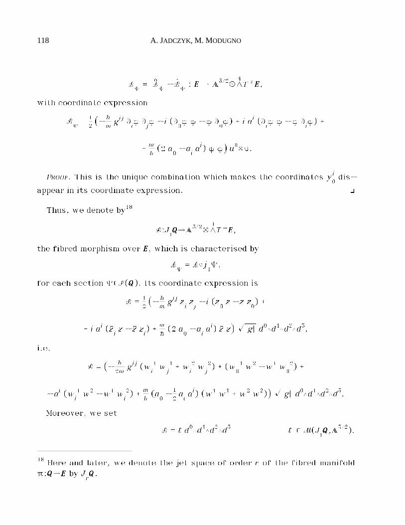
118 A. JADCZYK, M. MODUGNO
L„= °L
„- êL
„: EEEE é A
3/2ÆL4T*EEEE,
with coordinate expression
L„= 1
2⁄- h
mgij Ù
i㥠Ù
j¥ - i (Ù
0㥠¥ - 㥠Ù
0¥) _ i ai (Ù
i㥠¥ - 㥠Ù
i¥) _
_ mh(2 a
0- a
iai) 㥠¥^ u0æ¨.
PROOF. This is the unique combination which makes the coordinates yi0dis-
appear in its coordinate expression. ò
Thus, we denote by18
L:J1QQQQéA3/2ÆL
4T*EEEE,
the fibred morphism over EEEE, which is characterised by
L„= L©j
1„,
for each section „$S(QQQQ). Its coordinate expression is
L = 12⁄- h
mgij ãz
izj- i (ãz
0z - ãz z
0) _
_ i ai (ãziz - ãz z
i) _ m
h(2 a
0- a
iai) ãz z^ ÊÕ¡g¡ d0◊d1◊d2◊d3,
i.e.
L = ⁄- h
2mgij (w
i1 w
j1 _ w
i2 w
j2) _ (w
01 w2 - w1 w
02) _
- ai (wi1 w2 - w1 w
i2) _ m
h(a
0- 1
2aiai) (w1 w1 _ w2 w2)^ ÊÕ¡g¡ d0◊d1◊d2◊d3.
Moreover, we set
L = l d0◊d1◊d2◊d3 l $ M(J1QQQQ,A3/2).
18 Here and later, we denote the jet space of order r of the fibred manifoldπ:QQQQéEEEE by J
rQQQQ.
GALILEI GENERAL RELATIVISTIC QUANTUM MECHANICS 119
We stress that L is a real map.
AAAASSSSSSSSUUUUMMMMPPPPTTTTIIIIOOOONNNN QQQQ4444. We assume L to be the quantum Lagrangian responsibleof the quantum total equation. ò
Before analysing the consequences of this assumptions, we conclude thissection with a digression.
We prefer to develop the Lagrangian formalism directly on the quantumbundle. However, the reader may wish to develop an equivalent theory on thequantum principal bundle. Here, we just give a hint to find a distinguishedLagrangian on the quantum principal bundle.
Let PPPPéEEEE be the quantum principal bundle, i.e. the principal bundle withstructure group U(1), whose associated bundle is the quantum bundle QQQQéEEEE.Let ª:PPPPé· be the normal chart associated with the quantum gauge b.
LLLLEEEEMMMMMMMMAAAA IIIIIIII....2222....1111....2222. The form associated with the quantum connection on thequantum principal bundle is the fibred morphism
~c:J1EEEEEEEEPPPPéT*PPPP
with coordinate expression
~c= dª - i m
h(- 1
2gijy0i y
0j d0 _ g
ijy0i dj _ a
¬d¬).
Then, we obtain the fibred morphism over EEEE
Gc:J1EEEEEEEEPPPPéTÆ(T*PPPPÆ
EEEET*PPPP)
defined as
Gcˆ ~
cædt _ dtæ~
c,
with coordinate expression
Gc= u
0æ⁄dªæd0 _ d0ædª _
- i mh(- g
ijy0i y
0j d0æd0 _ g
ijy0i (djæd0 _ d0ædj) _ a
¬(d¬æd0 _ d0æd¬)^. ò
LLLLEEEEMMMMMMMMAAAA IIIIIIII....2222....1111....3333. The pullback of the vertical metric is the fibred mor-
120 A. JADCZYK, M. MODUGNO
phisms over EEEE
ª*g:J1EEEEéAÆMÆ(T*EEEEÆ
EEEET*EEEE)
with coordinate expression
ª*g = m gij(di - y
0i d0)æ(dj - y
0j d0).
Then, we obtain the fibred morphism over EEEE
GŸ:J1EEEEéTÆ(T*EEEEÆ
EEEET*EEEE)
defined as
GŸ ˆ mhhhhª*g,
with coordinate expression
GŸ = mhgiju0æ(di - y
0i d0)æ(dj - y
0j d0). ò
The two above objects live on J1EEEE, i.e. they are observer dependent. Next,
we show that there is a unique minimal coupling of them, which is pro-jectable on PPPP, i.e. observer independent.
TTTTHHHHEEEEOOOORRRREEEEMMMM IIIIIIII....2222....1111....2222. There is a unique combination of Gcand G&, which pro-
jects on PPPP; namely
G ˆ Gc- i GŸ : PPPPéTÆ(T*PPPPÆ
EEEET*PPPP),
with coordinate expression
G = u0æ⁄dªæd0 _ d0ædª - i m
h(g
ijdiædj _ 2 a
0d0æd0 _ a
i(diæd0 _ d0ædi)^.
Thus, G is a non-degenerate T-valued metric on the quantum principalbundle. ò
The above metric G yields naturally a Lagrangian on the quantum principalbundle, which is equivalent to the above Lagrangian L.
GALILEI GENERAL RELATIVISTIC QUANTUM MECHANICS 121
II.2.2. The quantum momentum
Next, we study the (observer independent) four dimensional quantummomentum. We follow two independent ways: we deduce it from theLagrangian formalism and from another geometrical construction based onthe differential of the quantum section.
DDDDEEEEFFFFIIIINNNNIIIITTTTIIIIOOOONNNN IIIIIIII....2222....2222....1111. The quantum momentum is defined to be the verticalderivative of L
VQQQQL :J
1QQQQéA3/2ÆTEEEEÆ
EEEEL4T*EEEEÆ
EEEEQQQQ*. ¡
PPPPRRRROOOOPPPPOOOOSSSSIIIITTTTIIIIOOOONNNN IIIIIIII....2222....2222....1111. The quantum momentum can be naturally regardedas a fibred morphism over EEEE
p:J1QQQQéT*ÆTEEEEÆ
EEEEQQQQ.
Then, for each „$S(QQQQ), we obtain the observer independent section
p„ˆ p©j
1„ : EEEE é T*ÆTEEEEÆ
EEEEQQQQ,
with coordinate expression
p„= u0æ⁄¥ Ù
0- i h
mgij (Ù
j¥ - i m
haj¥) Ù
i^æb.
PROOF. It follows by using the natural fibred isomorphisms19
i re(h):QQQQ*éQQQQ Ç ,ã¶:L4T*EEEEéT*ÆA*3/2ÆTEEEE. ò
We can recover geometrically the quantum momentum in the followingway.
LLLLEEEEMMMMMMMMAAAA IIIIIIII....2222....2222....1111. If „$S(QQQQ), then we have the following natural fibredmorphisms over EEEE
19 The conventional multiplicative factor i in the isomorphism QQQQ*éQQQQ has beenchosen in such a way to obtain an expression of momentum in agreement withProp. II.4.2.1.
122 A. JADCZYK, M. MODUGNO
ôp„ˆ dæ„ : J
1EEEE é T*ÆTEEEEÆ
EEEEQQQQ êp
„ˆ hhhh
mêı#„ : J
1EEEE é T*ÆTEEEEÆ
EEEEQQQQ,
with coordinate expressions
ôp„ˆ ¥ u0æ(Ù
0_ yi
0Ùi)æb êp
„ˆ hhhh
mgij ⁄Ù
j¥ - i (p
j/h) ¥^ Ù
iæb.
TTTTHHHHEEEEOOOORRRREEEEMMMM IIIIIIII....2222....2222....1111. If „$S(QQQQ), then p„
is the unique combination (up to a
scalar factor) of ôp„and êp
„, which projects over EEEE; namely,
p„= ôp
„- i êp
„: EEEE é T*ÆTEEEEÆ
EEEEQQQQ.
PROOF. This is the unique combination which makes the coordinates yi0dis-
appear in its coordinate expression. ò
We stress that the quantum momentum is an observer independent fourdimensional object.
The time component of the quantum momentum is defined without refer-ence to any observer; actually, it coincides with the quantum section itself.On the other hand, the choice of an observer allows us to define the space-like component of the quantum momentum.
CCCCOOOORRRROOOOLLLLLLLLAAAARRRRYYYY IIIIIIII....2222....2222....1111. For each „$S(QQQQ), we obtain the observer indepen-dent section
v„ˆ re h(„,p
„) : EEEE é T*ÆTEEEE.
Moreover, in the domain where „ does not vanish, the section
o„ˆ v
„/h(„,„) : EEEE é T*ÆTEEEE
projects over 1TTTT, hence it is an observer, with coordinate expression
o„= u0æ⁄Ù
0- re i h
mgij
ã¥(Ùj¥ - i m
haj¥)
h(„,„)Ùi^. ò
Thus, we have obtained a distinguished observer associated with „. It ispossible to interpret the physical meaning of this observer in agreement with
GALILEI GENERAL RELATIVISTIC QUANTUM MECHANICS 123
the uncertainty principle; in fact, we can assume that o„is determined ex-
perimentally only by means of a statistical procedure which involves manyparticles (see [Me]).
II.2.3. The generalised Schrödinger equation
Next, we study the (observer independent) quantum total equation. Wefollow two independent ways: we deduce it from the Lagrangian formalismand from another geometrical construction based on the differentials ofthe quantum section and momentum.
For this purpose, we need an intrinsic construction of the Euler-Lagrangeoperator. We shall follow the procedure of [Co].
RRRREEEEMMMMAAAARRRRKKKK IIIIIIII....2222....3333....1111. The quantum momentum can be regarded as a fibredmorphism over EEEE
P:J1QQQQéL
4T*QQQQ.
PROOF. It follows by applying to VQQQQL the natural linear fibred morphisms
Ç , ¶:TEEEEÆEEEEL4T*EEEEéL3T*EEEE ª
QQQQ*:J
1QQQQEEEEQQQQ*éT*QQQQ
over EEEE and J1EEEEéQQQQ, respectively. ò
RRRREEEEMMMMAAAARRRRKKKK IIIIIIII....2222....3333....2222. We obtain the fibred morphism over EEEE
E ˆ dL _ dhP : J
2QQQQ é A
3/2ÆL5T*QQQQ,
where d is the exterior differential and dhthe contact horizontal exterior
differential (see [Co]). ò
RRRREEEEMMMMAAAARRRRKKKK IIIIIIII....2222....3333....3333. By considering the linear epimorphism T*QQQQéV*QQQQ overQQQQ, E can be characterised by a fibred morphism over EEEE
êE:J2QQQQ é A
3/2ÆL4T*EEEEÆ
EEEEQQQQ*.
Moreover, by taking into account the real component of the Hermitian met-
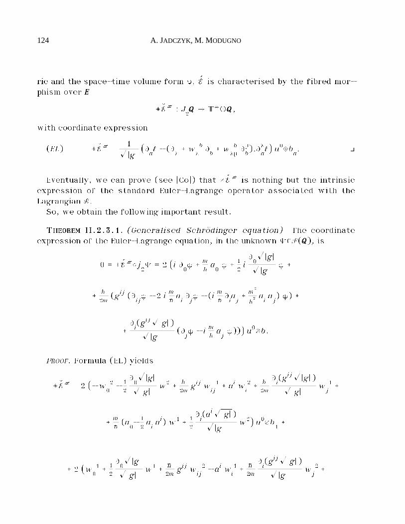
124 A. JADCZYK, M. MODUGNO
ric and the space-time volume form ¨, êE is characterised by the fibred mor-phism over EEEE
* êE# : J2QQQQ é T*ÆQQQQ,
with coordinate expression
(EL) * êE# =1
ÊÕ¡g¡⁄Ù
al - (Ù
¬_ w
¬b Ù
b_ w
¬bµÙµb).Ù¬
al^ u0æb
a. ò
Eventually, we can prove (see [Co]) that * êE# is nothing but the intrinsicexpression of the standard Euler-Lagrange operator associated with theLagrangian L.
So, we obtain the following important result.
TTTTHHHHEEEEOOOORRRREEEEMMMM IIIIIIII....2222....3333....1111. (Generalised Schrödinger equation) The coordinateexpression of the Euler-Lagrange equation, in the unknown „$S(QQQQ), is
0 = * êE#©j2„ = 2 ⁄i Ù
0¥ _ m
ha0¥ _ 1
2iÙ0ÊÕ¡g¡
ÊÕ¡g¡¥ _
_ h
2m(gij (Ù
ij¥ - 2 i m
haiÙj¥ - (i m
hÙiaj_ m
2
h2 ai aj) ¥) _
_Ùi(gijÊÕ¡g¡ )
ÊÕ¡g¡(Ùj¥ - i m
haj¥))^ u0æb.
PROOF. Formula (EL) yields
* êE# = 2 ⁄- w02 - 1
2
Ù0ÊÕ¡g¡
ÊÕ¡g¡w2 _ h
2mgij w
ij1 _ ai w
i2 _ h
2m
Ùi(gijÊÕ¡g¡ )
ÊÕ¡g¡wj1 _
_ mh(a
0- 1
2aiai) w1 _ 1
2
Ùi(aiÊÕ¡g¡ )
ÊÕ¡g¡w2^ u0æb
1_
_ 2 ⁄w01 _ 1
2
Ù0ÊÕ¡g¡
ÊÕ¡g¡w1 _ h
2mgij w
ij2 - ai w
i1 _ h
2m
Ùi(gijÊÕ¡g¡ )
ÊÕ¡g¡wj2 _
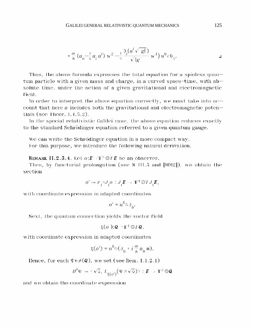
GALILEI GENERAL RELATIVISTIC QUANTUM MECHANICS 125
_ mh(a
0- 1
2aiai) w2 - 1
2
Ùi(aiÊÕ¡g¡ )
ÊÕ¡g¡w1^ u0æb
2. ò
Thus, the above formula expresses the total equation for a spinless quan-tum particle with a given mass and charge, in a curved space-time, with ab-solute time, under the action of a given gravitational and electromagneticfield.
In order to interpret the above equation correctly, we must take into ac-count that here a includes both the gravitational and electromagnetic poten-tials (see Theor. I.4.3.2).
In the special relativistic Galilei case, the above equation reduces exactlyto the standard Schrödinger equation referred to a given quantum gauge.
We can write the Schrödinger equation in a more compact way.For this purpose, we introduce the following natural derivation.
RRRREEEEMMMMAAAARRRRKKKK IIIIIIII....2222....3333....4444. Let o:EEEEéT*ÆTEEEE be an observer.Then, by functorial prolongation (see § III.3 and [MM2]), we obtain the
section
o' ˆ r1©J
1o : J
1EEEE é T*ÆTJ
1EEEE,
with coordinate expression in adapted coordinates
o' = u0æÙ0.
Next, the quantum connection yields the vector field
≈(o'):QQQQéT*ÆTQQQQ,
with coordinate expression in adapted coordinates
≈(o') = u0æ(Ù0_ i m
ha0i).
Hence, for each „$S(QQQQ), we set (see Rem. I.1.2.1)
Do„ ˆ Ç¢Ãã, L≈(o')
(„æ¢Ã)¶ : EEEE é T*ÆQQQQ
and we obtain the coordinate expression
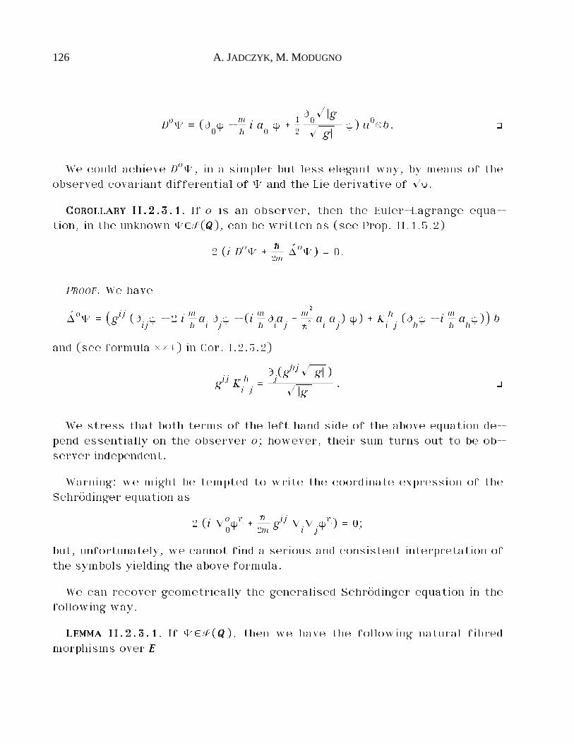
126 A. JADCZYK, M. MODUGNO
Do„ = (Ù0¥ - m
hi a
0¥ _ 1
2
Ù0ÊÕ¡g¡
ÊÕ¡g¡¥) u0æb. ò
We could achieve Do„, in a simpler but less elegant way, by means of theobserved covariant differential of „ and the Lie derivative of ¢Ã.
CCCCOOOORRRROOOOLLLLLLLLAAAARRRRYYYY IIIIIIII....2222....3333....1111. If o is an observer, then the Euler-Lagrange equa-tion, in the unknown „$S(QQQQ), can be written as (see Prop. II.1.5.2)
2 (i Do„ _ hhhh
2mêËo„) = 0.
PROOF. We have
êËo„ = ⁄gij (Ùij¥ - 2 i m
haiÙj¥ - (i m
hÙiaj_ m
2
h2 ai aj) ¥) _ Ki
hj(Ù
h¥ - i m
hah¥)^ b
and (see formula ***) in Cor. I.2.3.2)
gij Kihj=Ùj(ghjÊÕ¡g¡ )
ÊÕ¡g¡. ò
We stress that both terms of the left hand side of the above equation de-pend essentially on the observer o; however, their sum turns out to be ob-server independent.
Warning: we might be tempted to write the coordinate expression of theSchrödinger equation as
2 (i ıo0¥∆ _ h
2mgij ı
iıj¥∆) = 0;
but, unfortunately, we cannot find a serious and consistent interpretation ofthe symbols yielding the above formula.
We can recover geometrically the generalised Schrödinger equation in thefollowing way.
LLLLEEEEMMMMMMMMAAAA IIIIIIII....2222....3333....1111. If „$S(QQQQ), then we have the following natural fibredmorphisms over EEEE
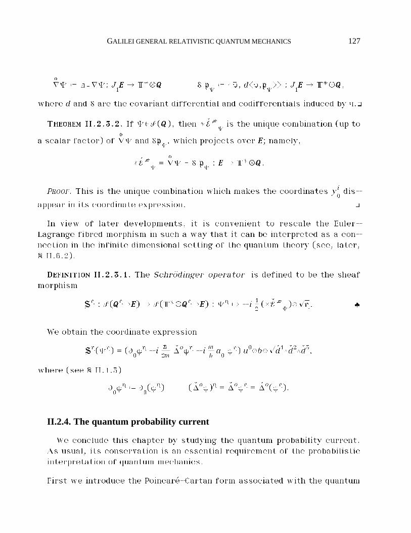
GALILEI GENERAL RELATIVISTIC QUANTUM MECHANICS 127
°ı„ ˆ dœı„: J1EEEE é T*ÆQQQQ ∂ p
„ˆ Çã, dǨ,p
㦦 : J
1EEEE é T*ÆQQQQ,
where d and ∂ are the covariant differential and codifferentials induced by c.ò
TTTTHHHHEEEEOOOORRRREEEEMMMM IIIIIIII....2222....3333....2222. If „$S(QQQQ), then * êE#„is the unique combination (up to
a scalar factor) of °ı„ and ∂p„, which projects over EEEE; namely,
* êE#„= °ı„ _ ∂ p
„: EEEE é T*ÆQQQQ.
PROOF. This is the unique combination which makes the coordinates yi0dis-
appear in its coordinate expression. ò
In view of later developments, it is convenient to rescale the Euler-Lagrange fibred morphism in such a way that it can be interpreted as a con-nection in the infinite dimensional setting of the quantum theory (see, later,§ II.6.2).
DDDDEEEEFFFFIIIINNNNIIIITTTTIIIIOOOONNNN IIIIIIII....2222....3333....1111. The Schrödinger operator is defined to be the sheafmorphism
S∆ : S(QQQQ∆éEEEE) é S(T*ÆQQQQ∆éEEEE) : „∆ ´ - i 12(* êE#
„)æ¢Ã∆. ¡
We obtain the coordinate expression
S∆(„∆) = (Ù0¥∆ - i h
2mêËo¥∆ - i m
ha0¥∆) u0æbæÊêd1◊êd2◊êd3,
where (see § II.1.5)
Ù0¥∆ ˆ Ù
0(¥∆) ( êËo¥)∆ = êËo¥∆ = êËo(¥∆).
II.2.4. The quantum probability current
We conclude this chapter by studying the quantum probability current.As usual, its conservation is an essential requirement of the probabilisticinterpretation of quantum mechanics.
First we introduce the Poincaré-Cartan form associated with the quantum
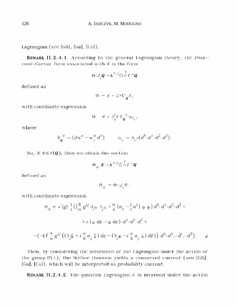
128 A. JADCZYK, M. MODUGNO
Lagrangian (see [GS], [Ga], [Co]).
RRRREEEEMMMMAAAARRRRKKKK IIIIIIII....2222....4444....1111. According to the general Lagrangian theory, the Poin-caré-Cartan form associated with L is the form
Ï:J1QQQQéA3/2ÆL
4T*QQQQ
defined as
Ï ˆ L _ ª◊VQQQQL,
with coordinate expression
Ï = L _ Ùa¬l ª
QQQQa׷
¬,
where
ªQQQQa ˆ (dwa - w
¬a d¬) ∑
¬ˆ Ù
¬œ(d0◊d1◊d2◊d3).
So, if „$S(QQQQ), then we obtain the section
Ï„:EEEEéA3/2ÆL
4T*QQQQ
defined as
Ï„ˆ Ï©j
1„.
with coordinate expression
Ï„= ÊÕ¡g¡ 1
2⁄⁄hmgij Ù
i㥠Ù
j¥ _ m
h(a
0- 1
2a2) 㥠¥^ d0◊d1◊d2◊d3 _
_ i (㥠dz - ¥ dãz)◊d1◊d2◊d3 _
- (-1)i hmgij ⁄(Ù
j㥠_ i m
hajã¥) dz _ (Ù
j¥ - i m
haj¥) dãz)^◊d0◊d1…◊âdi…◊d3^. ò
Then, by considering the invariance of the Lagrangian under the action ofthe group U(1), the Nöther theorem yields a conserved current (see [GS],[Ga], [Co]), which will be interpreted as probability current.
RRRREEEEMMMMAAAARRRRKKKK IIIIIIII....2222....4444....2222. The quantum Lagrangian L is invariant under the action
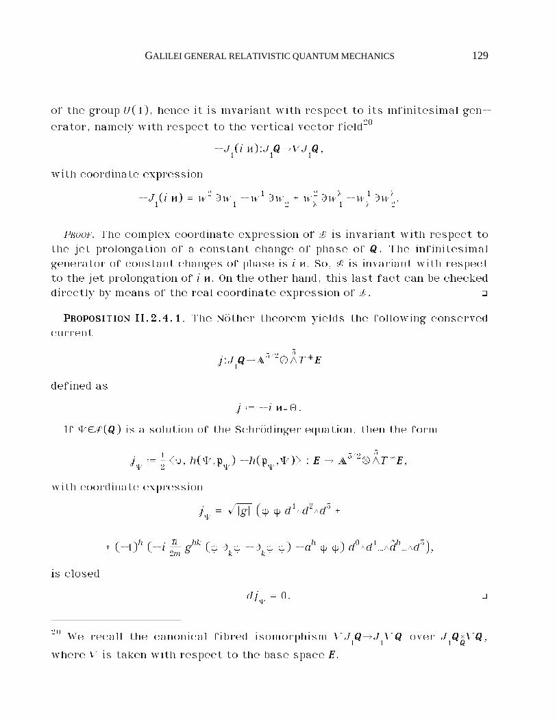
GALILEI GENERAL RELATIVISTIC QUANTUM MECHANICS 129
of the group U(1), hence it is invariant with respect to its infinitesimal gen-
erator, namely with respect to the vertical vector field20
- J1(i i):J
1QQQQéVJ
1QQQQ,
with coordinate expression
- J1(i i) = w2 Ùw
1- w1 Ùw
2_ w
¬2 Ùw¬
1- w
¬1 Ùw¬
2.
PROOF. The complex coordinate expression of L is invariant with respect tothe jet prolongation of a constant change of phase of QQQQ. The infinitesimalgenerator of constant changes of phase is i i. So, L is invariant with respectto the jet prolongation of i i. On the other hand, this last fact can be checkeddirectly by means of the real coordinate expression of L. ò
PPPPRRRROOOOPPPPOOOOSSSSIIIITTTTIIIIOOOONNNN IIIIIIII....2222....4444....1111. The Nöther theorem yields the following conservedcurrent
j:J1QQQQéA3/2ÆL
3T*EEEE
defined as
j ˆ - i iœÏ.
If „$S(QQQQ) is a solution of the Schrödinger equation, then the form
j„ˆ 1
2Ǩ, h(„,p
„) - h(p
„,„)¶ : EEEE é A
3/2ÆL3T*EEEE,
with coordinate expression
j„= ÊÕ¡g¡ ⁄㥠¥ d1◊d2◊d3 _
_ (-1)h (- i h
2mghk (㥠Ù
k¥ - Ù
k㥠¥) - ah 㥠¥) d0◊d1…◊âdh…◊d3^,
is closed
dj„= 0. ò
20 We recall the canonical fibred isomorphism VJ1QQQQéJ
1VQQQQ over J
1QQQQQQQQVQQQQ,
where V is taken with respect to the base space EEEE.
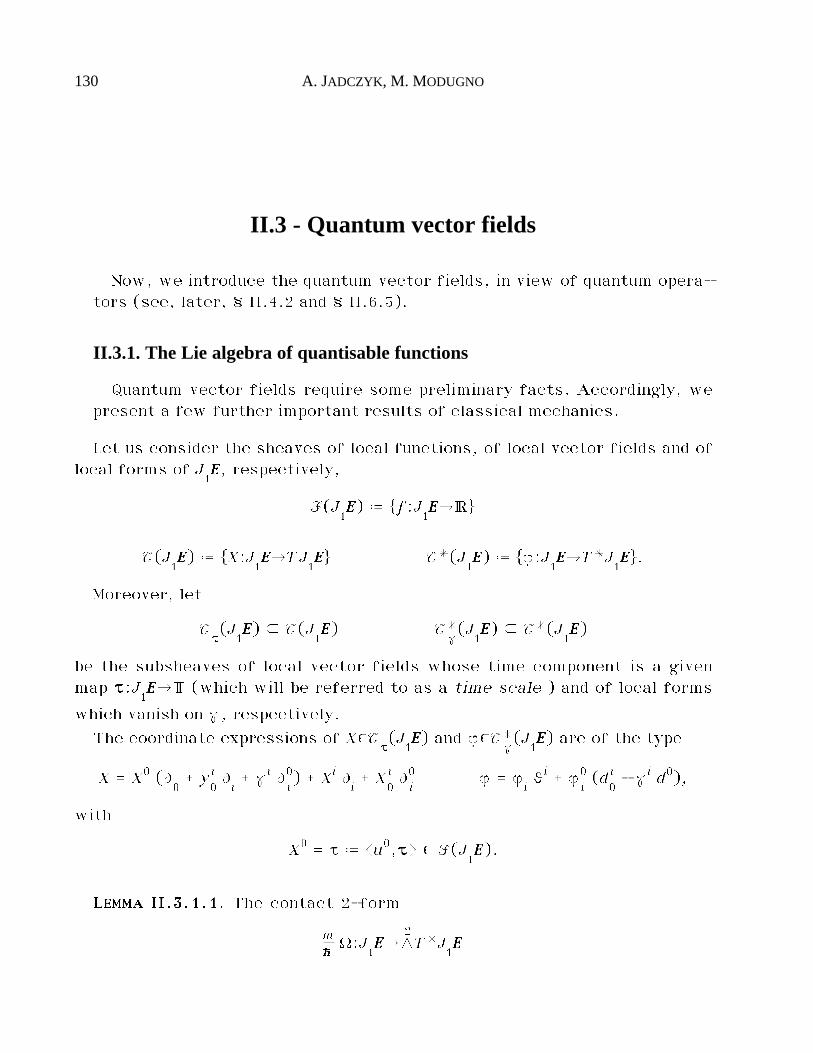
130 A. JADCZYK, M. MODUGNO
II.3 - Quantum vector fields
Now, we introduce the quantum vector fields, in view of quantum opera-tors (see, later, § II.4.2 and § II.6.3).
II.3.1. The Lie algebra of quantisable functions
Quantum vector fields require some preliminary facts. Accordingly, wepresent a few further important results of classical mechanics.
Let us consider the sheaves of local functions, of local vector fields and oflocal forms of J
1EEEE, respectively,
F(J1EEEE) ˆ f:J
1EEEEé·
T(J1EEEE) ˆ X:J
1EEEEéTJ
1EEEE T*(J
1EEEE) ˆ ƒ:J
1EEEEéT*J
1EEEE.
Moreover, let
T††††(J1EEEE) ç T(J
1EEEE) T*
˙(J1EEEE) ç T*(J
1EEEE)
be the subsheaves of local vector fields whose time component is a givenmap ††††:J
1EEEEéT (which will be referred to as a time scale ) and of local forms
which vanish on ˙, respectively.The coordinate expressions of X$T
††††(J1EEEE) and ƒ$T*
˙(J1EEEE) are of the type
X = X0 (Ù0_ y
0i Ù
i_ ˙i Ù
i0) _ Xi Ù
i_ X
0i Ù
i0 ƒ = ƒ
iªi _ ƒ
i0 (d
0i - ˙i d0),
with
X0 = † ˆ Çu0,††††¶ $ F(J1EEEE).
LLLLEEEEMMMMMMMMAAAA IIIIIIII....3333....1111....1111. The contact 2-form
mhhhhÒ:J
1EEEEéL
2T*J
1EEEE
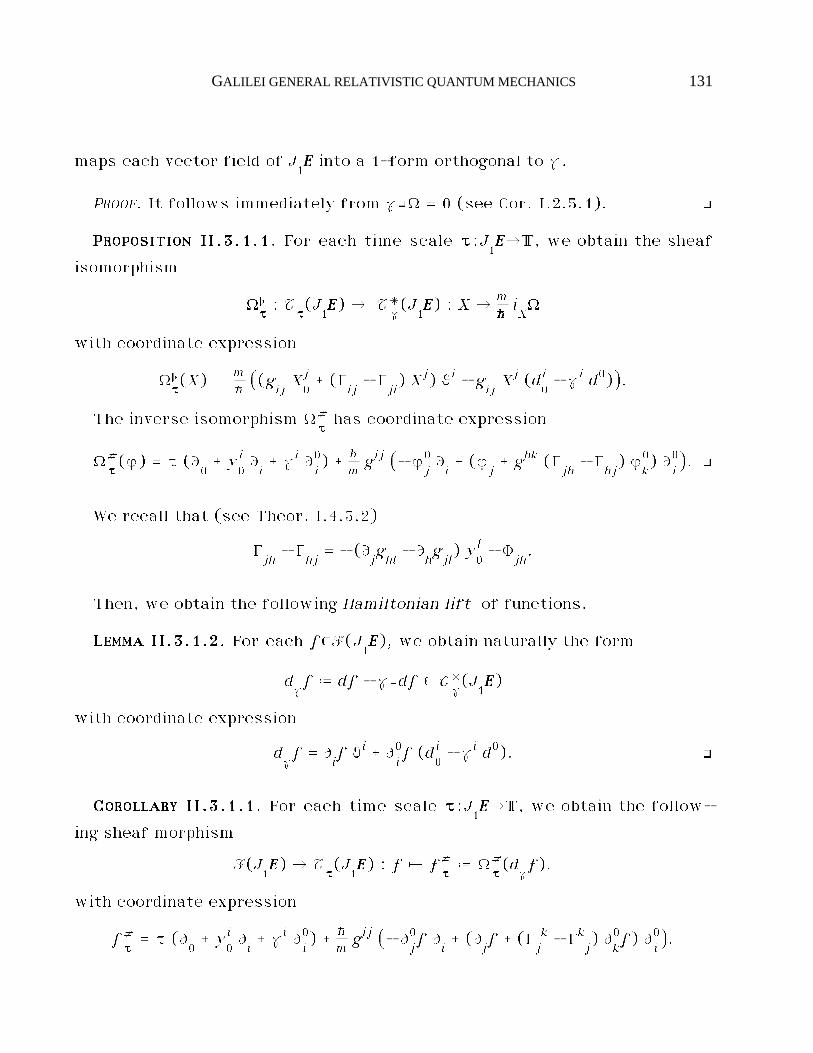
GALILEI GENERAL RELATIVISTIC QUANTUM MECHANICS 131
maps each vector field of J1EEEE into a 1-form orthogonal to ˙.
PROOF. It follows immediately from ˙œÒ = 0 (see Cor. I.2.5.1). ò
PPPPRRRROOOOPPPPOOOOSSSSIIIITTTTIIIIOOOONNNN IIIIIIII....3333....1111....1111. For each time scale ††††:J1EEEEéT, we obtain the sheaf
isomorphism
Ò††††@ : T
††††(J1EEEE) é T*
˙(J1EEEE) : X ´ m
hhhhiXÒ
with coordinate expression
Ò††††@(X) = m
h⁄(g
ijX0j _ (Í
ij- Í
ji) Xj) ªi - g
ijXj (d
0i - ˙i d0)^.
The inverse isomorphism Ò††††# has coordinate expression
Ò††††#(ƒ) = † (Ù
0_ y
0i Ù
i_ ˙i Ù
i0) _ h
mgij ⁄- ƒ0
jÙi_ (ƒ
j_ ghk (Í
jh- Í
hj) ƒ0
k) Ù
i0^. ò
We recall that (see Theor. I.4.3.2)
Íjh- Í
hj= - (Ù
jghl- Ù
hgjl) y
0l - È
jh.
Then, we obtain the following Hamiltonian lift of functions.
LLLLEEEEMMMMMMMMAAAA IIIIIIII....3333....1111....2222. For each f$F(J1EEEE), we obtain naturally the form
d˙f ˆ df - ˙œdf $ T*
˙(J1EEEE)
with coordinate expression
d˙f = Ù
if ªi _ Ù
i0f (d
0i - ˙i d0). ò
CCCCOOOORRRROOOOLLLLLLLLAAAARRRRYYYY IIIIIIII....3333....1111....1111. For each time scale ††††:J1EEEEéT, we obtain the follow-
ing sheaf morphism
F(J1EEEE) é T
††††(J1EEEE) : f ´ f
††††# ˆ Ò
††††#(d
˙f).
with coordinate expression
f††††# = † (Ù
0_ y
0i Ù
i_ ˙i Ù
i0) _ h
mgij ⁄- Ù0
jf Ù
i_ (Ù
jf _ (Í
jk - Ík
j) Ù0
kf) Ù
i0^.
132 A. JADCZYK, M. MODUGNO
We have the following properties
f††††# = ˙(††††) _ f
0#
(f' _ f")0# = f'
0# _ f"
0# (f' f")
0# = f' f"
0# _ f'
0# f". ò
The Hamiltonian lift yields the generalised Poisson Lie bracket.
PPPPRRRROOOOPPPPOOOOSSSSIIIITTTTIIIIOOOONNNN IIIIIIII....3333....1111....1111. The sheaf morphism
F(J1EEEE)˚F(J
1EEEE) é F(J
1EEEE) : (f', f") ´ f', f" ˆ m
hhhhif'0#if"0#Ò
is a Lie bracket.Its coordinate expression is
f',f" = h
mgij ⁄Ù
if' Ù0
jf" - Ù
i0f' Ù
jf" _ ghk (Í
jh- Í
hj) Ù0
kf' Ù
i0f"^.
PROOF. The proof can be achieved analogously to the standard case, butwith more difficulties, because we have to replace the standard d with d
˙. ò
This bracket has some interesting properties. In particular, we have
f',f"0# = [f'
0#,f"
0#].
However, this bracket has no relativistically covariant role in classicalmechanics.
On the other hand, we can prove the following important result based on acriterion of projectability for classical Hamiltonian lift, which later will playan essential role in quantum mechanics.
Let us consider the subsheaf of tube-like functions with respect to thefibring J
1EEEEéEEEE
Ft(J1EEEE) ç F(J
1EEEE).
PPPPRRRROOOOPPPPOOOOSSSSIIIITTTTIIIIOOOONNNN IIIIIIII....3333....1111....2222. If f$Ft(J
1EEEE), then the following conditions are
equivalent:
GALILEI GENERAL RELATIVISTIC QUANTUM MECHANICS 133
i) the vector field f††††# is projectable over EEEE;
ii) the function f is, with respect to the fibres of J1EEEEéEEEE, a polynomial of
degree 2, whose second derivative is of the form
ffff» mhhhhg : EEEE é (TÆT)ÆV*EEEEÆ
EEEEV*EEEE,
where
ffff» = ††††;
iii) the coordinate expression of f is of the following type
f = f» m2hgijy0i y
0j _ f
iy0i _ f
©f»,f
©,f
i$F(EEEE),
where
f» = †.
PROOF. The vector field f††††# is projectable if and only if
Ù0h† = 0 † Ù0
hy0i - h
mgij Ù0
h0jf = 0
i.e., if and only if
Ù0h† = 0 Ù
i00jf = † m
hgij
i.e. if and only if
†:EEEEé· f = † m2hgijy0i y
0j _ f
iy0i _ f
©. ò
Then, we introduce the following definition, for a reason which will beclear soon.
DDDDEEEEFFFFIIIINNNNIIIITTTTIIIIOOOONNNN IIIIIIII....3333....1111....1111. We define the quantisable functions to be the func-tions of the above type. ¡
If f is a quantisable function, then the associated time scale
†††† ˆ ffff» : EEEE é T
is said to be its time component.
134 A. JADCZYK, M. MODUGNO
If f is a quantisable function, then the corresponding projectable Hamilton-ian lift and the associated projection are denoted by
f# ˆ f††††# $ T
††††(J1EEEE) fH $ T
††††(EEEE).
Thus, given u0$T_*, we have implicitly set
f» ˆ Çu0,ffff»¶.
We stress that we have assumed no relation between f» ˆ † and f©.
RRRREEEEMMMMAAAARRRRKKKK IIIIIIII....3333....1111....2222. If f is a quantisable function, then we obtain the coor-dinate expression
f# = f» Ù0- h
mfi Ù
i_
_ gij ⁄12Ùjf» g
hky0h y
0k _ (h
mÙjfh_ h
m(Ù
kgjh- Ù
jghk) fk - f» Ù
0gjh) y
0h _
_ h
mÙjf©_ h
mÈhjfh _ f» È
j0^ Ù
i0,
hence
fH = f» Ù0- h
mfi Ù
i. ò
The quantisable functions constitute a sheaf, which is denoted by
Q(J1EEEE) ç F
t(J1EEEE).
Moreover, we shall be concerned with the subsheaves of quantisable func-tions whose time component is constant and of quantisable functions whosetime component vanishes
Qc(J1EEEE) ç Q(J
1EEEE) Q
0(J1EEEE) ç Q
c(J1EEEE).
RRRREEEEMMMMAAAARRRRKKKK IIIIIIII....3333....1111....1111. All functions f$F(EEEE), which depend only on space-time(for instance, the space-time coordinates), are quantisable functions.Moreover, all functions f$A(J
1EEEE),which are affine with respect to the fibring
J1EEEEéEEEE (for instance, the components of the classical momentum), are quan-
GALILEI GENERAL RELATIVISTIC QUANTUM MECHANICS 135
tisable functions. The remaining quantisable functions (for instance, theclassical kinetic energy, Hamiltonian and Lagrangian) have a quadratic termwith respect to the fibring J
1EEEEéEEEE, which is proportional to the metric,
through an arbitrary coefficient dependent only on space-time.Thus, we have the sheaf monomorphisms
F(EEEE) ç A(J1EEEE) ç Q(J
1EEEE). ò
TTTTHHHHEEEEOOOORRRREEEEMMMM IIIIIIII....3333....1111....2222. The sheaf Q(J1EEEE) is a sheaf of Lie algebras with re-
spect to the bracket
[f', f"] ˆ f', f" _ ˙(ffff'»).f" - ˙(ffff"»).f'.
Moreover, the sheaves Qc(J1EEEE) and Q
0(J1EEEE) are subsheaves of Lie algebras.
The coordinate expression of the above Lie bracket is given by
[f', f"] = ⁄f'» Ù0f"» - f"» Ù
0f'» - h
m(f'i Ù
if"» - f"i Ù
if'»)^ m
2hghky0h y
0k _
_ ghk⁄f'» Ù
0f"k - f"» Ù
0f'k - h
m(f'i Ù
if"k - f"i Ù
if'k)^ y
0h _
_ f'» Ù0f"
©- f"» Ù
0f'©- h
m(f'h Ù
hf"
©- f"h Ù
hf'©) _
_ (f'» f"h - f"» f'h) Èh0_ h
mf'h f"k È
hk.
PROOF. The explicit expression of the bracket follows from a long computa-tion in coordinates. Then, this expression shows that Q(J
1EEEE) is closed under
the above bracket.The Jacobi property could be checked by a very long direct computation in
coordinates. However, in the next section we can obtain an intrinsic proof asa corollary of an important result of the quantum theory (Cor. II.3.2.2). ò
CCCCOOOORRRROOOOLLLLLLLLAAAARRRRYYYY IIIIIIII....3333....1111....2222. The subsheaf A(J1EEEE) ç Q(J
1EEEE) is a subsheaf of Lie
algebras. ò
CCCCOOOORRRROOOOLLLLLLLLAAAARRRRYYYY IIIIIIII....3333....1111....3333. The sheaf morphism
136 A. JADCZYK, M. MODUGNO
H : Q(J1EEEE)éT(EEEE) : f´fH
is a morphsim of Lie algebras, i.e.
[f', f"]H = [f'H, f"H]. ò
EEEEXXXXAAAAMMMMPPPPLLLLEEEE IIIIIIII....3333....1111....1111. We have the following Hamiltonian lifts
(x0)H = 0 (yl)H = 0
(pi/h)H = - Ù
i(H/h)H = Ù
0(L/h)H = Ù
0- ai Ù
i. ò
EEEEXXXXAAAAMMMMPPPPLLLLEEEE IIIIIIII....3333....1111....2222. We have the following brackets
[x0, f] = - f» [yi, f] = h
mfi
[pi/h, p
j/h] = 0 [H/h, p
i/h] = m
hÈ0i. ò
II.3.2. The Lie algebra of quantum vector fields
In this section, we show how the geometrical structure of the quantumbundle yields naturally a distinguished Lie algebra of vector fields, whichwill be called quantum vector fields. Moreover, we exhibit a natural Lie al-gebra isomorphism between quantisable functions and quantum vectorfields.
Later, the quantum vector fields will be the source of quantum operators(see, later, § II.4.2 and § II.6.3).
We start by considering the vector fields of QQQQŸ, which preserve the basicquantum structures. We need to start from this bundle, because the quantumconnection lives on it.
We need the covariant differential of a vector field, which is a particularcase of the differential of tangent valued forms defined in [Mo2], [Mo3] (seealso § III.5). We stress that this differential cannot be understood neither inthe sense of linear connections on a manifold, nor in the sense of derivationlaws.
GALILEI GENERAL RELATIVISTIC QUANTUM MECHANICS 137
RRRREEEEMMMMAAAARRRRKKKK IIIIIIII....3333....2222....1111. Let p:FFFFéBBBB be a fibred manifold and
c:FFFFéT*BBBBÆFFFFTFFFF
a connection. If X:FFFFéTFFFF is a vector field projectable on X:BBBBéTBBBB, then itscovariant differential is defined to be the vertical valued 1-form
dcX ˆ [c,X] : FFFF é T*BBBBÆ
FFFFVFFFF,
where [ , ] is the Frölicher-Nijenhuis bracket, given by
(dcX)(u) = [c(u), X] - c([u, X]), Åu$T(BBBB),
and with coordinate expression
dcX = (- Ù
¬Xµ c
µi - Ù
µc¬i Xµ _ Ù
¬Xi _ c
¬j Ù
jXi - Ù
jc¬i Xj) d¬æÙ
i.
Moreover, we recall the formula
(R) dc(c(X)) = - 2 XœR
c,
where Rc:FFFFéL
2T*BBBBÆ
FFFFVFFFF is the curvature of c. ò
Next, let p:FFFFéBBBB be a line bundle. Then, a projectable vector field X is saidto be Hermitian if it is (real) linear over its projection X and preserves theHermitian product. A Hermitian vector field turns out to be also complex lin-ear. The coordinate expression of a Hermitian vector field X is of the type
X = X¬ Ù¬_ i f i f, X¬$F(BBBB).
Then, we introduce the following concept.
DDDDEEEEFFFFIIIINNNNIIIITTTTIIIIOOOONNNN IIIIIIII....3333....2222....1111. An upper quantum vector field is defined to be a
(tube-like) vector field21
XŸ:QQQQŸéTQQQQŸ
which
21 Here, the arrow “Ÿ” in XŸ does not refer to any pullback of a possiblesection X, but just reminds the pullback bundle QQQQŸ.
138 A. JADCZYK, M. MODUGNO
i) projects onto a (local) vector field
XŸ:J1EEEEéTJ
1EEEE,
ii) is Hermitian complex linear over XŸ,iii) has a TTTT-horizontal covariant differential, i.e.
dcXŸ : QQQQŸ é J
1EEEEEEEE(T*ÆQQQQ) ç T*J
1EEEE ÆJ1EEEEQQQQŸ. ¡
dcXŸ = ˙œd
cXŸ. ¡
Condition iii) can be reformulated in a useful way through ˙.
RRRREEEEMMMMAAAARRRRKKKK IIIIIIII....3333....2222....2222. Condition iii) is clearly equivalent to
pr©dcXŸ = 0,
where pr:T*J1EEEEéV*J
1EEEE is the canonical linear epimorphism over J
1EEEE.
Thus, condition iii) reads in coordinates as
dc iXŸ = 0 d
c i0XŸ = 0.
Moreover, condition iii) is equivalent to
iii)' dcXŸ = ˙œd
cXŸ. ò
The upper quantum vector fields constitute a sheaf and the upper quantumvector fields, with a given time component ††††:J
1EEEEéT, constitute a subsheaf,
which are denoted by
Q(QQQQŸ) ç T(QQQQŸ) Q††††(QQQQŸ) ç Q(QQQQŸ).
The above sheaves are not closed with respect to the Lie bracket.On the other hand, the upper quantum vector fields can be classified, up to
the choice of an arbitrary time scale, by the functions of the classical jetspace, through the following formula.
TTTTHHHHEEEEOOOORRRREEEEMMMM IIIIIIII....3333....2222....1111. For each time scale ††††:J1EEEEéT, we have an ·-linear
sheaf isomorphism
GALILEI GENERAL RELATIVISTIC QUANTUM MECHANICS 139
qŸ††††: F(J
1EEEE) é Q
††††(QQQQŸ) : f ´ XŸ
f,††††
given by
(U) XŸf,††††
ˆ c(f††††#) _ i f i.
PROOF. 1) Let XŸ be an upper quantum vector field whose time-component is†††† and let us prove that it is of the type
XŸ ˆ c(f††††#) _ i f i,
for some function f$F(J1EEEE).
Let us decompose XŸ into its horizontal and vertical components
(c) XŸ = c(XŸ) _ ~c(XŸ).
Conditions i) and ii) imply that ~c(XŸ) is of the type
(v) ~c(XŸ) = i f i, f$F(J
1EEEE).
Therefore, condition iii)' can be written as
iii)" i (df - ˙.f)æi = ˙œdc(c(XŸ)) - d
c(c(XŸ)).
Moreover, formulas (R) and (Rc) (see Rem. II.3.2.1) yield
dc(c(XŸ)) = - 2 i m
hhhhXŸœÒæi.
Hence, condition iii)" can be written as
(df - ˙.f) = Ò@††††(XŸ)
i.e.
h) XŸ = f††††#.
Thus, formulas (c), (v) and (h) yield
XŸ = c(f††††#) _ i f i
2) Conversely, if f$F(J1EEEE), then analogous computations prove that for-
mula (U) yields an upper quantum vector field, whose time-component is ††††. ò
140 A. JADCZYK, M. MODUGNO
PPPPRRRROOOOPPPPOOOOSSSSIIIITTTTIIIIOOOONNNN IIIIIIII....3333....2222....1111. The coordinate expression of XŸf,††††
is
XŸf,††††
= † (Ù0_ y
0i Ù
i_ ˙i Ù
i0) _
_ h
mgij ⁄- Ù0
jf Ù
i_ (Ù
jf _ ghk (Í
jh- Í
hj) Ù0
kf) Ù
i0^ _
_ i ⁄f _ † L/h - h
mgij (p
j/h) Ù0
if^ i. ò
Formula (U) clearly recalls a well known formula of geometric quantisation(see, for instance, [St], [Wo]). However, there are important differencesbetween our approach and geometric quantisation; they are basically relatedto the general covariance and the role of time. In particular, we shall seethat an important difference will arise later in the construction of the quan-tum operator associated with energy. Indeed, we stress that our upperquantum vector fields need not to be time-vertical.
The above formula looks nice, but we have got two problems. In fact, wehave been forced to search for distinguished vector fields on QQQQŸ and not on QQQQ,just because the quantum connection lives on QQQQŸ. But, these vector fieldsmap sections of QQQQ into sections of QQQQŸ. This problem can be solved if, addi-tionally, the above vector fields are projectable over EEEE. Moreover, the aboveisomorphism depends on the choice of a time scale and we need a reasonablecriterion to make this choice. Luckily, the two problems can be solved to-gether. In fact, we can prove the following result.
If XŸ:QQQQŸéTQQQQŸ is any vector field, then the canonical fibred epimorphismpr:TQQQQŸéTQQQQ yields the fibred morphism over QQQQ
X ˆ pr©XŸ : J1EEEEEEEEQQQQ é TQQQQ.
The vector field XŸ is said to be projectable over EEEE if X can be written as
X:QQQQéTQQQQ.
TTTTHHHHEEEEOOOORRRREEEEMMMM IIIIIIII....3333....2222....2222. If XŸf,††††
is an upper quantum vector field, then the fol-
lowing conditions are equivalent:i) XŸ
f,††††is projectable over EEEE;
GALILEI GENERAL RELATIVISTIC QUANTUM MECHANICS 141
ii) f is a quantisable function and its time component is ††††.
PROOF. i) £ ii). We can prove the assertion directly.If XŸ
f,††††is projectable over EEEE, then
Ù0h† = 0 † Ù0
hy0i - h
mgij Ù0
h0jf = 0
i.e.
Ù0h† = 0 Ù
i00jf = † m
hgij
i.e.
†:EEEEé· f = † m2hgijy0i y
0j _ f
iy0i _ f
©.
On the other hand we obtain the same result as a consequence of the theo-rem concerning the projectability of the Hamiltonian lift of functions (seeProp. II.3.1.2).
ii) £ i). We can easily see that all components of Xf,††††
, including the imagi-
nary component, do not depend on the coordinates y0i. ò
DDDDEEEEFFFFIIIINNNNIIIITTTTIIIIOOOONNNN IIIIIIII....3333....2222....2222. A quantum vector field is defined to be the vectorfield
X:QQQQéTQQQQ
associated with a projectable upper quantum vector field XŸ. ¡
The quantum vector fields constitute a sheaf, which is denoted by
Q(QQQQ) ç T(QQQQ).
Moreover, we shall be concerned with the subsheaves of quantum vectorfields with constant and vanishing time component
Qc(QQQQ) ç Q(QQQQ) Q
0(QQQQ) ç Q
c(QQQQ).
So, we are in the position to achieve the following important formula.
CCCCOOOORRRROOOOLLLLLLLLAAAARRRRYYYY IIIIIIII....3333....2222....1111. The coordinate expression of the quantum vector
142 A. JADCZYK, M. MODUGNO
field associated with the quantisable function
f = f» m2hgijy0i y
0j _ f
iy0i _ f
©
is
Xf= f» Ù
0- h
mfi Ù
i_ i (m
hf» a
0- fi a
i_ f
©) i.
PROOF. It follows from the coordinate expression of XŸ and f. ò
CCCCOOOORRRROOOOLLLLLLLLAAAARRRRYYYY IIIIIIII....3333....2222....2222. The map
q : Q(J1EEEE) é Q(QQQQ) : f ´ X
f
is a sheaf linear isomorphism. In particular, Qc(J1EEEE) and Q
0(J1EEEE) are isomor-
phic, respectively, to Qc(QQQQ) and Q
0(QQQQ). ò
Eventually, we can prove the following important result.
LLLLEEEEMMMMMMMMAAAA IIIIIIII....3333....2222....1111. The sheaf Q(QQQQ) of quantum vector fields and the sub-sheaves Q
c(QQQQ) and Q
0(QQQQ) of quantum vector fields with constant and vanish-
ing time component are closed under the Lie bracket.
PROOF. It follows from a long computation in coordinates. ò
TTTTHHHHEEEEOOOORRRREEEEMMMM IIIIIIII....3333....2222....3333. The map (see Theor. II.3.1.2)
Q(J1EEEE) é Q(QQQQ) : f ´ X
f
is an isomorphism of sheaves of Lie algebras.Namely, for each k$·, f,f',f"$Q(J
1EEEE), we have
Xkf= k X
fXf'_f"
= Xf'_ X
f"
[Xf', X
f"] = X
[f', f"]. ò
GALILEI GENERAL RELATIVISTIC QUANTUM MECHANICS 143
II.4 - Quantum Lie operators
In this chapter, we show how the quantum vector fields act naturally onthe quantum sections and yield a Lie algebra of operators, which will becalled quantum Lie operators. Moreover, we exhibit a natural Lie algebraisomorphism between quantisable functions and quantum Lie operators.
This is our first approach to the subject of quantum operators and to theprinciple of correspondence; in this step, the classical Hamiltonian corre-sponds to the time derivative. A further development of the theory will beachieved later in the framework of the quantum Hilbert bundle (see §II.6.3); in this context, the classical Hamiltonian will correspond to thestandard operator, naturally generalised to our curved space-time.
The quantum vector fields act naturally on the quantum sections as Liederivatives; so, we might introduce the quantum operators directly in thisway. The result would be quite interesting; but, in order to obtain sym-metric (possibly self-adjoint) operators (see § II.6.3), we need a littlemore complicated approach. Namely, we have to consider quantum half-densities. More precisely, in the space-like integration procedure (see §II.6.1), we shall be involved with space-like half-densities. On the otherhand, in the construction of operators, we need to consider space-timehalf-densities.
II.4.1. Lie operators
This section is devoted to a preliminary discussion about the action oflinear projectable vector fields on quantum densities.
First, we introduce the notion of Lie derivative of sections of a vectorbundle.
Let p:FFFFéBBBB be a vector bundle.
RRRREEEEMMMMAAAARRRRKKKK IIIIIIII....4444....1111....1111. A vertical vector field Y:FFFFéVFFFFˆFFFFBBBBFFFF is said to be basic
if it projects over a section s:BBBBéFFFF through the following commutative dia-gram
144 A. JADCZYK, M. MODUGNO
FFFF äY
VFFFF ˆ FFFFBBBBFFFF
p ï ï pr2
BBBBáäs
FFFF
Conversely each section s:BBBBéFFFF can be regarded as a basic vertical vectorfield Y:FFFFéVFFFF, which is projectable over the section itself. This correspon-dence between sections and basic vector fields is a bijection. ò
LLLLEEEEMMMMMMMMAAAA IIIIIIII....4444....1111....1111. Let X:FFFFéTFFFF be a linear projectable vector field and let usdenote its projection by X:BBBBéTBBBB.
For each section s:BBBBéFFFF, the Lie bracket
[X,s]:FFFFéVFFFF
is a basic vector field, hence determines the section
X.s ˆ [X,s] : BBBB é FFFF,
with coordinate expression
X.s = (X¬ Ù¬si - Xi
jsj) b
i. ò
So, if X:FFFFéTFFFF is a linear projectable vector field, then we define the as-sociated Lie operator as the sheaf morphism
X. : S(FFFF) é S(FFFF) : s ´ X.s.
LLLLEEEEMMMMMMMMAAAA IIIIIIII....4444....1111....2222. The map
X ´ X.
is injective. Moreover, the map
(X,s) ´ X.s
has the following properties
X.(s_s') = X.s _ X.s' X.(fs) = f (X.s) _ X.f s
(X _ X').s = X.s _ X'.s (fX).s = f (X.s)
[X., X'.](s) ˆ X.X'.s - X'.X.s = [X,X'].s
GALILEI GENERAL RELATIVISTIC QUANTUM MECHANICS 145
for each linear projectable vector field X,X':FFFFéTFFFF, section s,s':BBBBéFFFF andfunction f:BBBBé·. ò
We can re-interpret the above results in terms of connections.If we assume a linear connection
c:FFFFéT*BBBBÆBBBBTFFFF
on the vector bundle p:FFFFéBBBB, then we have the following result.
LLLLEEEEMMMMMMMMAAAA IIIIIIII....4444....1111....3333. Let X:BBBBéTBBBB be a vector field and consider its horizontalprolongation
X ˆ Xœc : FFFF é TFFFF,
which is linear over its projection X.Then, for each section s:BBBBéFFFF, we obtain the formula
X.s = ıXs,
with coordinate expression
X.s = (X¬ Ù¬si - Xi
jsj) b
i= X¬ (Ù
¬si - c
¬ijsj) b
i= ı
Xs. ò
Now, let us apply the above results to our quantum framework.
PPPPRRRROOOOPPPPOOOOSSSSIIIITTTTIIIIOOOONNNN IIIIIIII....4444....1111....1111. Let X:QQQQéTQQQQ be a linear projectable vector fieldand let us denote its projection by X:EEEEéTEEEE. Then, we obtain, via the aboveLie derivative, the sheaf morphism
X. : S(QQQQ) é S(QQQQ) : „ ´ [X, „].
Moreover, we obtain, via a standard Lie derivative, the sheaf morphism
X. : S(ÊL4T*EEEE) é S(ÊL
4T*EEEE) : ¢Ã ´ L(X)¢Ã,
which depends only on X.Hence, we can extend, via the Leibnitz rule, the Lie derivative to the
space-time densities and obtain the sheaf morphism
X. : S(QQQQ¨) é S(QQQQ¨) : „ ´ X.„¨ ˆ [X, „]æ¢Ã_ „æL(X)¢Ã.
Furthermore, let X:QQQQéVQQQQ be a linear vertical vector field. Then, in an
146 A. JADCZYK, M. MODUGNO
analogous way, we obtain, via a vertical Lie derivative, the sheaf morphism
X. : S(QQQQ∆) é S(QQQQ∆) : „ ´ X.„∆ ˆ [X, „]æ¢Ã∆ _ „æL(X)¢Ã∆. ò
PPPPRRRROOOOPPPPOOOOSSSSIIIITTTTIIIIOOOONNNN IIIIIIII....4444....1111....2222. If X,X':QQQQéTQQQQ are linear projectable vector fields,
and we consider their action both on S(QQQQ¨) and S(QQQQ∆), then the standardidentity for the commutator of Lie derivatives yields
[X., X'.] = [X, X']. . ò
II.4.2. The general Lie algebras isomorphism
So, we are in the position to introduce the quantum Lie operators and theLie algebra isomorphism between quantisable functions and quantum Lieoperators.
DDDDEEEEFFFFIIIINNNNIIIITTTTIIIIOOOONNNN IIIIIIII....4444....2222....1111. Let f$Q(J1EEEE) be a quantisable function and X
f$Q(QQQQ)
the corresponding quantum vector field. Then, the quantum Lie operator as-sociated with f is defined to be the sheaf morphism
Yfˆ i X
f. : S(QQQQ∆) é S(QQQQ∆) : „∆ ´ i (X
f.„¨)æ 1
¢Ãæ¢Ã∆. ¡
We have already explained why we apply Xfto S(QQQQ∆) and not directly to
S(QQQQ): we consider „∆ in view of the integration on the fibres of space-timeand of the symmetry of the quantum Lie operator (see § II.6.3). Moreover,
we are forced to pass through „¨ because, in the general case, the action ofXfon ¢Ã∆ is not defined. Furthermore, the reason of the multiplication by the
imaginary unit will appear later (see § II.6.3), when we prove the symmetryof the quantum operators.
RRRREEEEMMMMAAAARRRRKKKK IIIIIIII....4444....2222....1111. In the particular case when the quantisable function f isaffine with respect to the fibres of J
1EEEEéEEEE, hence the quantum vector field
Xfis vertical, we obtain, more directly,
Yf= i X
f. : S(QQQQ∆) é S(QQQQ∆) : „∆ ´ i X
f.„∆. ò
GALILEI GENERAL RELATIVISTIC QUANTUM MECHANICS 147
The quantum Lie operators constitute a sheaf, which is denoted by
L(QQQQ∆).
Moreover, we shall be concerned with the subsheaves of quantum Lie op-erators corresponding to quantisable functions with constant and vanishingtime component
Lc(QQQQ∆) ç L(QQQQ∆) L
0(QQQQ∆) ç L
c(QQQQ∆).
LLLLEEEEMMMMMMMMAAAA IIIIIIII....4444....2222....1111. The map
Q(J1EEEE) é L(QQQQ∆) : f ´ Y
f
is a sheaf isomorphism. ò
LLLLEEEEMMMMMMMMAAAA IIIIIIII....4444....2222....2222. The sheaf L(QQQQ∆) is a sheaf of Lie algebras with respectto the bracket
L(QQQQ∆)˚L(QQQQ∆) é L(QQQQ∆) : (Yf', Y
f") ´ [Y
f', Y
f"] ˆ - i (Y
f'©Y
f"- Y
f"©Y
f').
Moreover, Lc(QQQQ∆) and L
0(QQQQ∆) are subsheaves of Lie algebras. ò
So, we are in the position to state the following important result.
TTTTHHHHEEEEOOOORRRREEEEMMMM IIIIIIII....4444....2222....1111. The map
Q(J1EEEE) é L(QQQQ∆) : f ´ Y
f
is an isomorphism of sheaves of Lie algebras.Namely, for each k$·, f,f',f"$Q(J
1EEEE), we have
Ykf= k Y
fYf'_f"
= Yf'_ Y
f"
[Yf', Y
f"] = Y
[f', f"]. ò
PPPPRRRROOOOPPPPOOOOSSSSIIIITTTTIIIIOOOONNNN IIIIIIII....4444....2222....1111. For each observer o, the action of the quantum Lie
operator Yfon „∆ is given by
Yf(„∆) = i (fHœıo„)∆ _ ⁄f©o _ i 1
2(div fH)^ „∆,
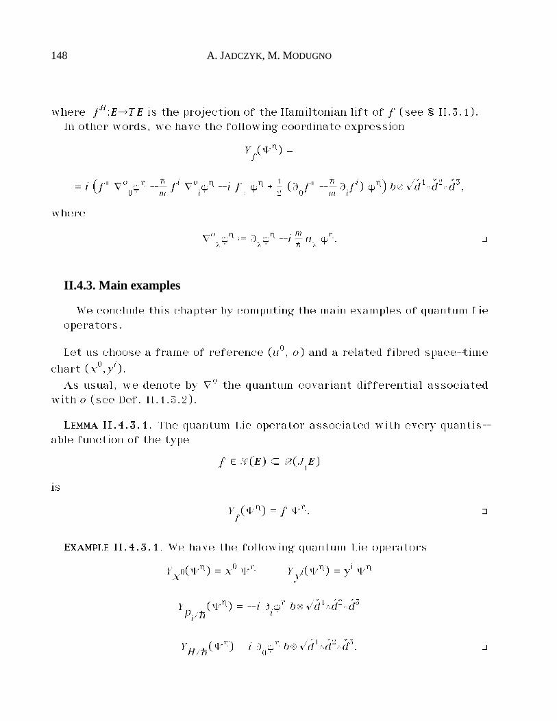
148 A. JADCZYK, M. MODUGNO
where fH:EEEEéTEEEE is the projection of the Hamiltonian lift of f (see § II.3.1).In other words, we have the following coordinate expression
Yf(„∆) =
= i ⁄f» ıo0¥∆ - h
mfi ıo
i¥∆ - i f
©¥∆ _ 1
2(Ù
0f» - h
mÙifi) ¥∆^ bæÊêd1◊êd2◊êd3,
where
ıo¬¥∆ ˆ Ù
¬¥∆ - i m
ha¬¥∆. ò
II.4.3. Main examples
We conclude this chapter by computing the main examples of quantum Lieoperators.
Let us choose a frame of reference (u0, o) and a related fibred space-time
chart (x0,yi).As usual, we denote by ıo the quantum covariant differential associated
with o (see Def. II.1.5.2).
LLLLEEEEMMMMMMMMAAAA IIIIIIII....4444....3333....1111. The quantum Lie operator associated with every quantis-able function of the type
f $ F(EEEE) ç Q(J1EEEE)
is
Yf(„∆) = f „∆. ò
EEEEXXXXAAAAMMMMPPPPLLLLEEEE IIIIIIII....4444....3333....1111. We have the following quantum Lie operators
Yx0(„∆) = x0 „∆ Yyi(„
∆) = yi „∆
Ypi/h
(„∆) = - i Ùi¥∆ bæÊêd1◊êd2◊êd3
YH/h(„∆) = i Ù
0¥∆ bæÊêd1◊êd2◊êd3. ò
GALILEI GENERAL RELATIVISTIC QUANTUM MECHANICS 149
EEEEXXXXAAAAMMMMPPPPLLLLEEEE IIIIIIII....4444....3333....2222. For each quantisable function f, we have
[Yx0, Yf] = - f» [Yyi, Yf] =h
mfi.
Moreover, we have
[Ypi/h
, Yx0] = 0 [Ypi/h
, Yyj] = - ∂ij [Yp
i/h, YH/h] = 0. ò
150 A. JADCZYK, M. MODUGNO
II.5 - Systems of double fibred manifolds
In view of further developments of the quantum theory, we need somepreliminary notions and results concerning the system associated with adouble fibred manifold. The theory of finite dimensional systems has beenextensively studied in [ MM], [Mo2 ] and has been already used in this paper(see § II.1.3). In this chapter, we introduce the infinite dimensional sys-tem of all smooth sections by means of a functorial construction.
II.5.1. The system
We start by introducing the notion of system of sections associated witha double fibred manifold and studying its basic properties.
First we need a few preliminaries about the concept of smoothness due toFrölicher and the notion of fibred set.
We shall be concerned with some sets constructed geometrically fromsome functional spaces. We could define a topology in order to achieve astructure of infinite dimensional manifold on such sets; but great difficultieswould arise. On the other hand the concept of smoothness due to Frölicher([Fr]) is very suitable for our purposes, as it allows us to achieve the geo-metrical constructions that we need, avoiding all troubles related to infinitedimensionality.
DDDDEEEEFFFFIIIINNNNIIIITTTTIIIIOOOONNNN IIIIIIII....5555....1111....1111. A smooth space in the sense of Frölicher (see [Fr],[Sl]), can be defined as a pair
(SSSS,C),
where SSSS is a set and
C ˆ c:·éSSSS
is a set of curves which will be called smooth.If (SSSS,C) and (SSSS',C') are smooth spaces, then a map f:SSSSéSSSS' is said to be
smooth if, for each smooth curve c:·éSSSS, the curve
GALILEI GENERAL RELATIVISTIC QUANTUM MECHANICS 151
c' ˆ f©c : · é SSSS'
is smooth. ¡
In particular, each classical manifold MMMM becomes a smooth space by as-suming as smooth curves, in the sense of Frölicher, just the smooth curves inthe classical sense. Then, it can be proved (see [CCKM], [Bo]) that a mapbetween classical manifolds is smooth in the classical sense if and only if itis smooth in the sense of Frölicher.
If (SSSS,C) is a smooth space, then by abuse of language we shall also saythat SSSS is a smooth space.
If SSSS and SSSS' are smooth spaces, then SSSS˚SSSS' becomes a smooth space in anatural way.
A fibred set is defined to be a set SSSS together with a surjective map
ß:SSSSéBBBB
of SSSS onto a set BBBB. When BBBB is a manifold, we denote by
S€(SSSSéBBBB)
the sheaf of local sections of the fibred set ß:SSSSéBBBB. Moreover, if SSSS is asmooth space, then we denote by
S(SSSSéBBBB) ç S€(SSSSéBBBB)
the subsheaf of smooth local sections of the fibred set ß:SSSSéBBBB.
Now, let us consider a (smooth) double fibred manifold
FFFF äqEEEE ä
pBBBB
and denote the typical double fibred charts of FFFF by
(x¬, yi, za) 1≤¬≤m, 1≤i≤l, 1≤a≤n.
We denote by
St€(FFFFéEEEEéBBBB) and S
t(FFFFéEEEEéBBBB)
the sheaf of tube-sections which are smooth along the fibres but possiblynon-smooth with respect to the base space BBBB and the subsheaf of smoothtube-sections.
152 A. JADCZYK, M. MODUGNO
DDDDEEEEFFFFIIIINNNNIIIITTTTIIIIOOOONNNN IIIIIIII....5555....1111....2222. The system associated with the double fibredmanifold FFFFéEEEEéBBBB is defined to be the pair
(ß:SFFFFéBBBB, ™),
wherei) SFFFF is the set
SFFFF ˆ øx$BBBB
SxFFFF,
where
SxFFFF ˆ „
x:EEEExéFFFF
x
denotes the set of smooth fibre-sections related to x$BBBB;ii) ß is the natural surjective map
ß : SFFFF é BBBB : „x´ x;
iii) ™ is the evaluation fibred morphism over EEEE
™ : SFFFFBBBBEEEE é FFFF : („
x, y) ´ „
x(y). ¡
RRRREEEEMMMMAAAARRRRKKKK IIIIIIII....5555....1111....1111. The evaluation fibred morphism ™ yields the naturalsheaf isomorphism
™™™™ : S€(SFFFFéBBBB) é St€(FFFFéEEEEéBBBB) : â„ ´ „ ˆ ™™™™( â„) ˆ ™© â„Ÿ,
where “Ÿ” denotes the pullback.The inverse natural sheaf isomorphism is
™™™™-1 : St€(FFFFéEEEEéBBBB) é S€(SFFFFéBBBB) : „ ´ â„,
where
â„ : x ´ „xˆ „
¡EEEEx
. ò
Next, we introduce a smooth structure in the sense of Frölicher on the setSFFFF by the following definition (see also [Ko]).
DDDDEEEEFFFFIIIINNNNIIIITTTTIIIIOOOONNNN IIIIIIII....5555....1111....3333. A curve âc:·éSFFFF is said to be smooth, in the senseof Frölicher, if the induced maps
GALILEI GENERAL RELATIVISTIC QUANTUM MECHANICS 153
ß©âc:·éBBBB c : (ß©âc)*EEEEéFFFF : y¬´âc(¬)(y
¬)
are smooth in the classical sense. ¡
RRRREEEEMMMMAAAARRRRKKKK IIIIIIII....5555....1111....2222. If MMMM is a manifold, then we can easily prove that a mapâc:MMMMéSFFFF is smooth in the sense of Frölicher if and only if the induced maps
ß©âc:MMMMéBBBB c:(ß©âc)*EEEEéFFFF
are smooth in the classical sense.Moreover, if SSSS' is a further smooth space, then we can easily prove that
the map f:SFFFFéSSSS' is smooth in the sense of Frölicher if and only if, for eachsmooth map âc:MMMMéSFFFF, the map
f©âc:MMMMéSSSS'
is smooth in the sense of Frölicher. ò
PPPPRRRROOOOPPPPOOOOSSSSIIIITTTTIIIIOOOONNNN IIIIIIII....5555....1111....1111. The maps ß and ™ turn out to be smooth.Moreover, a local section
â„:BBBBéSFFFF
of the fibred set SFFFFéBBBB turns out to be smooth if and only if the associatedtube-section
„ ˆ ™™™™( â„) : EEEE é FFFF
is smooth.Thus, the sheaf isomorphism ™™™™ restricts to a sheaf isomorphism
™™™™:S(SFFFFéBBBB)éSt(FFFFéEEEEéBBBB). ò
The following remark has an important role in the following (see § II.6.1).
RRRREEEEMMMMAAAARRRRKKKK IIIIIIII....5555....1111....3333. Let (ß':S'FFFFéBBBB, ™') be the subsystem of (ß:SFFFFéBBBB, ™)constituted by any subset of smooth-fibre sections of the double fibredmanifold FFFFéEEEEéBBBB. Then, all above constructions can be easily repeated forthis subsystem. Moreover, the inclusion S'FFFFàSFFFF turns out to be a smoothmap in the sense of Frölicher. ò
154 A. JADCZYK, M. MODUGNO
II.5.2. The tangent prolongation of the system
We pursue our presentation of systems by studying the tangent space ofthe system and the tangent prolongation of sections. We refer to the dou-ble fibred manifold and the associated system as in the previous section.
In order to define the tangent space of the smooth space SFFFF let us studythe tangent map of smooth curves ·éSFFFF.
LLLLEEEEMMMMMMMMAAAA IIIIIIII....5555....2222....1111. i) Let
âc:·éSFFFF
be a smooth curve defined in a neighbourhood of 0$·. Let us consider the in-duced curves
ß©âc:·éBBBB c:(ß©âc)*EEEEéFFFF
and set (see § III.2)
x ˆ (ß©âc)(0) $ BBBB u ˆ Ù(ß©âc) ˆ T(ß©âc)(0,1) $ TxBBBB â„
xˆ âc(0).
Then, the restriction of the tangent map Tc:T(ß©âc)*TEEEEéTFFFF to the fibre
over (0,1)$·˚· turns out to be an affine fibred morphism over â„x
Èuˆ Ùc ˆ Tc
¡(0,1): (TEEEE)
ué (TFFFF)
u,
whose fibre derivative is the linear fibred morphism over â„x
DÈu= T( â„
x) : (VEEEE)
xé (VFFFF)
x.
In other words, if v$(TEEEE)u, then we can write
Èu: (TEEEE)
ué (TFFFF)
u: (v _ w) ´ È
u(v) _ T( â„
x)(w) Åw$(VEEEE)
x.
We have the coordinate expression
(yi, za; îx¬, îyi, îza)©Èu= (yi, „
xa; u¬, îyi, È
ua _ Ù
i„xa îyi),
with
u¬ = Ùc¬ $ · Èua = Ùca : EEEE
xé ·.
GALILEI GENERAL RELATIVISTIC QUANTUM MECHANICS 155
ii) Conversely, let
x $ BBBB u $ TxBBBB â„
x$ S
xFFFF
and
Èu:(TEEEE)
ué(TFFFF)
u
be a map of the above type. Then, we can prove (see [CK]) that there is asmooth curve âc:·éSFFFF, such that
Ùc = Èu. ò
Then, we are led to the following definition.
DDDDEEEEFFFFIIIINNNNIIIITTTTIIIIOOOONNNN IIIIIIII....5555....2222....1111. The tangent space of the smooth space SFFFF is de-fined to be the set
TSFFFF ˆ øâ„x$SFFFF
T â„xSFFFF,
where
T â„xSFFFF ˆ È
u
is the set of smooth sections of the type
Èu:(TEEEE)
ué(TFFFF)
u, u$T
xBBBB, xˆß( â„
x)$BBBB,
such that Èuis an affine fibred morphism over â„
xand its fibre derivative is
the linear fibred morphism over â„x
DÈu= T( â„
x) : (VEEEE)
xé (VFFFF)
x. ¡
The basic geometrical constructions which hold for the tangent space ofthe standard finite dimensional manifolds can be repeated in our “infinite di-mensional” case.
PPPPRRRROOOOPPPPOOOOSSSSIIIITTTTIIIIOOOONNNN IIIIIIII....5555....2222....1111. We have the natural surjective maps
πSFFFF: TSFFFF é SFFFF : È
u´ â„
x, x ˆ π
BBBB(u),
156 A. JADCZYK, M. MODUGNO
and
Tß : TSFFFF é TBBBB : Èu´ u.
For each â„x$SFFFF, the tangent space T â„x
SFFFF of SFFFF at â„xturns out to be a
vector space in a natural way.Namely, if
Èu, È'
u', È"
u"$ T
â¥x
SFFFF ¬ $ ·,
then
¬ È'u'$ (T
â¥x
SFFFF)¬u'
È'u'_ È"
u"$ (T
â¥x
SFFFF)u'_u"
are well defined by
(¬ Èu) : (TEEEE)
¬ué (TFFFF)
¬u: (¬ v _ ¬ w) ´ ¬ È
u(v) _ T( â„
x)(¬ w)
(È'u'_ È"
u") : (TEEEE)
u'_u"é (TFFFF)
u'_u":
: (v' _ v" _ w) ´ È'u'(v') _ È"
u"(v") _ T( â„
x)(w) Åw$(VEEEE)
x
where v$(TEEEE)u, v'$(TEEEE)
u', v"$(TEEEE)
u".
Hence, the map Tß turns out to be a linear fibred morphism over ß. ò
RRRREEEEMMMMAAAARRRRKKKK IIIIIIII....5555....2222....1111. We have the natural evaluation fibred morphism over TEEEE
T™ : TSFFFFTBBBBTEEEE é TFFFF : (È
u, v) ´ È
u(v).
Thus, (Tß:TSFFFFéTBBBB, T™) turns out to be a subsystem of the system asso-ciated with the double fibred manifold TFFFFéTEEEEéTBBBB.
Therefore, all results of the above section apply to this subsystem. ò
RRRREEEEMMMMAAAARRRRKKKK IIIIIIII....5555....2222....2222. The vector structure of the fibred set TSFFFFéSFFFF turnsout to be smooth in the sense that the fibred morphisms over SFFFF
÷:·˚TSFFFFéTSFFFF _:TSFFFF˚TSFFFFéTSFFFF
are smooth. ò
We can define the tangent map of sections of the space of fibred sectionsin the following way.
GALILEI GENERAL RELATIVISTIC QUANTUM MECHANICS 157
RRRREEEEMMMMAAAARRRRKKKK IIIIIIII....5555....2222....3333. If â„$S(SFFFFéBBBB), then
T„:TEEEEéTFFFF
yields the smooth tube-section
âT„ ˆ (T™™™™)-1(T„) : TBBBB é TSFFFF. ò
DDDDEEEEFFFFIIIINNNNIIIITTTTIIIIOOOONNNN IIIIIIII....5555....2222....2222. The tangent prolongation of the section â„$S(SFFFFéBBBB)
is defined to be the section T â„$S(TSFFFFéTBBBB) given by
T â„ ˆ âT„. ¡
II.5.3. Connections on the system
We conclude this chapter by introducing the notion of a connection on oursystem. We still refer to the double fibred manifold and the associatedsystem as in the first section.
Analogously to the finite dimensional case (see § III.2), we have the exactsequence over SFFFF
0 ä VSFFFF äTSFFFF äSFFFF ˚BBBBT BBBB ä0.
DDDDEEEEFFFFIIIINNNNIIIITTTTIIIIOOOONNNN IIIIIIII....5555....3333....1111. A connection of the fibred set SFFFFéBBBB is defined to
be a smooth splitting22 âk of the above sequence, i.e. a smooth section
âk:SFFFFBBBBTBBBBéTSFFFF,
which is linear over SFFFF and is projectable over 1BBBB:TBBBBéTBBBB. ¡
We can interpret a connection âk as an operator which acts on the tube-sections of the double fibred manifold FFFFéEEEEéBBBB, in the following way.
PPPPRRRROOOOPPPPOOOOSSSSIIIITTTTIIIIOOOONNNN IIIIIIII....5555....3333....1111. Let âk be a connection.
If â„$S(SFFFFéBBBB), then, we obtain the section
22 k is a Chinese character, whose romanization in Pinyin is “kE”.
158 A. JADCZYK, M. MODUGNO
k(„):TEEEEéTFFFF,
given by the composition
TEEEE äâ„Ÿ
SFFFFBBBBTEEEE ä
âkŸTSFFFF
T BBBBTä
T™TFFFF,
with coordinate expression
(x¬, yi, za; îx¬, îyi, îza)©k(„) = (x¬, yi, „a; îx¬, îyi, kµa(„) îxµ _ Ù
j„a îyj),
where
kµa(„) $ F(EEEE).
Moreover, we obtain the smooth section
âk(„) = âk( â„) : TBBBB é TSFFFF.
Therefore, the sheaf morphism
k : St(FFFFéEEEEéBBBB) é S
t(TFFFFéTEEEEéTBBBB) : „ ´ k(„)
characterises âk itself. ò
A connection âk induces the covariant differential in the standard way.
LLLLEEEEMMMMMMMMAAAA IIIIIIII....5555....3333....1111. Let âk be a connection and â„$S(SFFFFéBBBB). Then, the map
T â„ - âk© â„Ÿ : TBBBB é TSFFFF
takes its values in VSFFFF, is projectable over â„ and is a linear fibred morphism
over â„. Hence, it can be can regard as a smooth section
ıâkâ„ ˆ T â„ - âk© â„Ÿ : BBBB é T*BBBBÆ
SFFFFVSFFFF,
which is projectable over â„. ò
DDDDEEEEFFFFIIIINNNNIIIITTTTIIIIOOOONNNN IIIIIIII....5555....3333....2222. Let âk be a connection. Then, the covariant differen-
tial of â„$S(SFFFFéBBBB) is defined to be the smooth local section
ıâkâ„ ˆ T â„ - âk© â„Ÿ : BBBB é T*BBBBÆ
SFFFFVSFFFF. ¡
GALILEI GENERAL RELATIVISTIC QUANTUM MECHANICS 159
We can interpret the covariant differential ıâkâ„ in terms of the tube-sec-
tion „, in the following way.
PPPPRRRROOOOPPPPOOOOSSSSIIIITTTTIIIIOOOONNNN IIIIIIII....5555....3333....2222. Let k be a connection and â„$S(SFFFFéBBBB). Then, themap
T„ - k(„) : TEEEE é TFFFF
is a smooth linear tube-fibred morphism over „, which factorizes through asmooth linear tube-fibred morphism over „
ık„:EEEE
BBBBTBBBBéVFFFF;
conversely, the map ık„ characterises T„ - k(„).
Moreover, we have
ıâkâ„ = âT„-k(„) : BBBB é T*BBBBÆ
SFFFFVSFFFF.
The coordinate expression of ık„ is
ık„ = ⁄Ù
¬„a - k
µa(„)^ dµæ(Ù
a©„). ò
A connection âk is said to be of order k if, for each smooth tube-section„:EEEEéFFFF, the map k(„) depends on „ through its vertical jet up to order k.
Now, let us consider the case when FFFFéEEEE is a vector bundle, hence SFFFFéBBBBand TSFFFFéTBBBB turn out to be smoothly equipped with a vector structure ontheir fibres.
The connection k is said to be linear if it is linear as a fibred morphismover BBBB. In other words, the connection k is linear if the operator
k : St(FFFFéEEEEéBBBB) é S
t(TFFFFéTEEEEéTBBBB) : „ ´ k(„)
is linear.
PPPPRRRROOOOPPPPOOOOSSSSIIIITTTTIIIIOOOONNNN IIIIIIII....5555....3333....3333. Let âk be a connection of order k. Then, the coordi-nate expression of the linear operator k:„´k(„) is of the type
kµa(„) = k
µab„b _ k
µajbÙj„b _ … _ k
µaj1…jk
bÙj1…j
k
„b,
160 A. JADCZYK, M. MODUGNO
where
(c) kµab, k
µajb, … , k
µaj1…jk
b$ F(EEEE).
Thus, in the linear case, the coordinate expression of ık„ is of the type
ık„ = (Ù
µ„a - k
µab„b - k
µajbÙj„b - … - k
µaj1…jk
bÙj1…j
k
„b) dµæÙa .
Thus, the equation
ık„ = 0,
in the unknown section „$St(FFFFéEEEEéBBBB), turns out to be a linear differential
equation of order k in the fibre derivatives and of order 1 in the base deriva-tives of „. ò
We observe that for any arbitrary choice of the above coefficients (c), weobtain a local connection. Hence global connections can be obtained by meansof the partition of unity.
We finish this chapter by observing that all above geometrical construc-tions are compatible, in a natural way, with restrictions to the subsystemassociated with a subsheaf of the sheaf of smooth tube-sections (see Rem.II.5.1.3). In particular, we shall be concerned with the subsystem of com-pact support tube-sections, on a vector double fibred manifold.
GALILEI GENERAL RELATIVISTIC QUANTUM MECHANICS 161
II.6 - The infinite dimensional quantum system
So far, the quantum theory has been developed on the quantum bundle QQQQ,which is based over the space-time EEEE (except for a temporary extension ofthe base space to J
1EEEE) and has one dimensional complex fibres.
On the other hand, the theory of systems suggests to translate the mainconcepts and results of the above quantum theory in terms of a new bundle
SQQQQ∆ which is based over the time TTTT and has infinite dimensional complexfibres.
Such a geometrical development of our quantum theory yields interestingphysical results and interpretations. In particular, it yields the Hilbertbundle and the generalisation to a curved space-time of the standardHamiltonian quantum operator and commutators.
II.6.1. The quantum system
We start by introducing the system associated with the double fibredmanifold of quantum space-like densities (see § II.1.2), according to theideas of the previous chapter.
So, we consider the system
(ß:SQQQQ∆éTTTT, ™)
associated with the double fibring
QQQQ∆ äπ∆EEEE ä
tTTTT.
In order to be able to perform integrations over the fibres of SQQQQƎTTTT, weneed to consider the subsystem of sections with compact support. So doing,we miss sections of physical interest, but they can be recovered later bymeans of a completion procedure. So, we introduce the following definition.
DDDDEEEEFFFFIIIINNNNIIIITTTTIIIIOOOONNNN IIIIIIII....6666....1111....1111. The pre-quantum system is defined to be the sub-system
162 A. JADCZYK, M. MODUGNO
(ßc:ScQQQQ∆éTTTT, ™c)
where
ScQQQQ∆ ˆ ø†$TTTT
Sc†QQQQ∆ ç SQQQQ∆,
and
Sc†QQQQ∆ ç S
†QQQQ∆ ˆ „∆
†:EEEE†éQQQQ∆
†
is the subset of sections with compact support. ¡
Let f:EEEEéÛ is a tube-function such that, for each †$TTTT, its restrictionf†:EEEE
†éÛ, has compact support; then we define the “space-like partial inte-
gral” of f as
|f ∆ : TTTT é Û : † ´ (|f ∆)(†) ˆ|EEEE†
f†∆†.
PPPPRRRROOOOPPPPOOOOSSSSIIIITTTTIIIIOOOONNNN IIIIIIII....6666....1111....1111. On the fibres of ßc:ScQQQQ∆éTTTT, we obtain the A3/2-valued Hermitian structure, given by
hâ : ScQQQQ∆BBBBScQQQQ∆ é ÛÆA3/2 : (È∆
†, „∆
†) ´ ÇÈ∆
†¡ „∆
†¶ ˆ|
EEEE†
h (Ȇ, „
†) ∆
†. ò
Hence, ßc:ScQQQQ∆éTTTT turns out to be a pre-Hilbert fibred set. Moreover, bycompletion (fibre by fibre), we obtain a Hilbert fibred set
HQQQQƎTTTT.
By abuse of language, we say that ScQQQQƎTTTT is the pre-Hilbert quantum bun-
dle and HQQQQƎTTTT the Hilbert quantum bundle.
II.6.2. The Schrödinger connection on the quantum system
Next, we re-interpret the Schrödinger operator in the present frame-work (see Def. II.2.3.1) and study its basic properties.
TTTTHHHHEEEEOOOORRRREEEEMMMM IIIIIIII....6666....2222....1111. There is a unique linear connection
GALILEI GENERAL RELATIVISTIC QUANTUM MECHANICS 163
âk:SQQQQ∆éT*ÆTSQQQQ∆
on the vector fibred set ß:SQQQQ∆éTTTT, such that the Schrödinger operator S∆ canbe written as
ık= S∆.
The coordinate expression of k is given by
k0(„∆) = i ( h
2mêËo¥∆ _ m
ha0¥∆).
PROOF. It follows immediately from a comparison of coordinate expressions
of ıkand S∆. ò
We can easily see that the connection k restricts to the subsystem
ßc:ScQQQQ∆éTTTT.
RRRREEEEMMMMAAAARRRRKKKK IIIIIIII....6666....2222....1111. Let o be an observer. Then, the observed verticalLaplacian can be regarded as a fibred morphism over TTTT
êËo:SQQQQ∆éSQQQQ∆.
Moreover, we can easily see that êËo restricts to the subsystem
ßc:ScQQQQ∆éTTTT. ò
LLLLEEEEMMMMMMMMAAAA IIIIIIII....6666....2222....1111. Let o be an observer. Then, the observed vertical
Laplacian is Hermitian. Namely, for each âÈ∆, â„∆$S(ScQQQQ∆éTTTT), we have
Ç êËo âÈ∆ ¡ â„∆¶ = Ç âÈ∆ ¡ êËo â„∆¶.
PROOF. We have
gij ( ÃıoiÃıo
jム¥ _ K
ihjÃıo
hム¥ - ムıo
iıo
j¥ - ムK
ihjıo
h¥) =
= gij ⁄ Ãıoi( Ãıo
jム¥) _ K
ihjÃıo
hム¥ - Ãıo
jムÙ
i¥ _
- ıoi(ムıo
j¥) - ムK
ihjıo
h¥ _ Ù
iムıo
j¥^ =
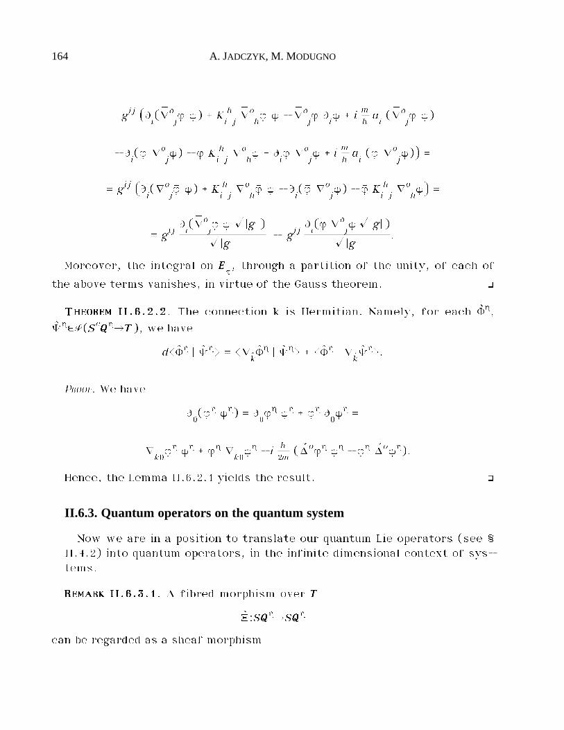
164 A. JADCZYK, M. MODUGNO
= gij ⁄Ùi( Ãıo
jム¥) _ K
ihjÃıo
hム¥ - Ãıo
jムÙ
i¥ _ i m
hai( Ãıo
jム¥)
- Ùi(ムıo
j¥) - ムK
ihjıo
h¥ _ Ù
iムıo
j¥ _ i m
hai(ムıo
j¥)^ =
= gij ⁄Ùi( Ãıo
jム¥) _ K
ihjÃıo
hム¥ - Ù
i(ムıo
j¥) - ムK
ihjıo
h¥^ =
= gijÙi( Ãıo
jム¥ ÊÕ¡g¡ )
ÊÕ¡g¡- gij
Ùi(ムıo
j¥ÊÕ¡g¡ )
ÊÕ¡g¡.
Moreover, the integral on EEEE†, through a partition of the unity, of each of
the above terms vanishes, in virtue of the Gauss theorem. ò
TTTTHHHHEEEEOOOORRRREEEEMMMM IIIIIIII....6666....2222....2222. The connection k is Hermitian. Namely, for each âÈ∆,â„∆$S(ScQQQQ∆éTTTT), we have
dÇ âÈ∆ ¡ â„∆¶ = ÇıâkâÈ∆ ¡ â„∆¶ _ Ç âÈ∆ ¡ ıâk
â„∆¶.
PROOF. We have
Ù0(ãƒ∆ ¥∆) = Ù
0ãƒ∆ ¥∆ _ ãƒ∆ Ù
0¥∆ =
= Ãık0ãƒ∆ ¥∆ _ ãƒ∆ ı
k0¥∆ - i h
2m( êËà oãƒ∆ ¥∆ - ãƒ∆ êËo¥∆).
Hence, the Lemma II.6.2.1 yields the result. ò
II.6.3. Quantum operators on the quantum system
Now we are in a position to translate our quantum Lie operators (see §II.4.2) into quantum operators, in the infinite dimensional context of sys-tems.
RRRREEEEMMMMAAAARRRRKKKK IIIIIIII....6666....3333....1111. A fibred morphism over TTTT
âÚ:SQQQQ∆éSQQQQ∆
can be regarded as a sheaf morphism
GALILEI GENERAL RELATIVISTIC QUANTUM MECHANICS 165
âÚ. : S(SQQQQ∆éTTTT) é S(SQQQQ∆éTTTT) : â„∆ ´ âÚ. â„∆ ˆ âÚ© â„∆.
Moreover, âÚ yields the sheaf morphism
Ú:S(QQQQ∆éEEEE)éS(QQQQ∆éEEEE),
characterised by
âÚ(„∆) = âÚ. â„∆.
The map
âÚ ´ Ú
is a bijection. ò
Henceforth, in order to deal with objects globally defined on the fibres oft:EEEEéTTTT, we need to restrict our attention to quantisable functions, which aretube-like with respect to the fibring J
1EEEEéTTTT.
We shall denote the corresponding sheaves by
Qt(J1EEEE) ç Q(J
1EEEE) Q
tc(J1EEEE) ç Q
c(J1EEEE) Q
t0(J1EEEE) ç Q
0(J1EEEE)
Lt(QQQQ∆) ç L(QQQQ∆) L
tc(QQQQ∆) ç L
c(QQQQ∆) L
t0(QQQQ∆) ç L
0(QQQQ∆).
PPPPRRRROOOOPPPPOOOOSSSSIIIITTTTIIIIOOOONNNN IIIIIIII....6666....3333....1111. Let f$Qt(J
1EEEE) and consider Y
f$L
t(QQQQ∆).
Then, we obtain the sheaf morphism
âYf: S(SQQQQ∆éTTTT) é S(SQQQQ∆éTTTT) : â„∆ ´ âY
f„∆. ò
CCCCOOOORRRROOOOLLLLLLLLAAAARRRRYYYY IIIIIIII....6666....3333....1111. In the particular case when f$Qt0(J
1EEEE), âY
facts
pointwisely on the sections of SQQQQƎTTTT, hence it can be regarded as a localfibred morphism over TTTT
âYf:SQQQQ∆éSQQQQ∆. ò
If f" = 0, then âYfis a differential operator of first order on the sections of
SQQQQƎTTTT.However, we are looking for a pointwise operator for all quantisable func-
166 A. JADCZYK, M. MODUGNO
tions. We shall solve the problem again by means of a criterion of pro-jectability, according to the following important result.
TTTTHHHHEEEEOOOORRRREEEEMMMM IIIIIIII....6666....3333....1111. For any f$Qt(J
1EEEE), the sheaf morphism
âÚfˆ âY
f- i ffff»œıâk
: S(SQQQQ∆éTTTT) é S(SQQQQ∆éTTTT)
acts pointwisely on the sections of SQQQQƎTTTT, hence it can be regarded as a lo-cal fibred morphism over TTTT
âÚfˆ âY
f- i ffff»œıâk
: SQQQQ∆ é SQQQQ∆.
Its coordinate expression is
Úf(„∆) =
= ⁄fo¥∆ _ i 1
2(Ù
0f» - h
mÙifi) ¥∆ - i h
mfi ıo
i¥∆ - f» h
2mêËo¥∆^ bæÊêd1◊êd2◊êd3.
In the particular case when f$Qt0(J1EEEE), we recover
âÚfˆ âY
f. ò
Of course, the above operator Úfis intrinsic, by construction. However,
we stress that its coordinate expression cannot be easily guessed by meansof standard arguments of differential geometry. Actually, this result is a“miracle” produced by the specific structure of the quantum bundle and itsquantum connection.
Then, we are led to introduce the following definition.
DDDDEEEEFFFFIIIINNNNIIIITTTTIIIIOOOONNNN IIIIIIII....6666....3333....1111. A quantum operator is defined to be the local fibredmorphism over TTTT
âÚfˆ âY
f- i ffff»œ âı
k: SQQQQ∆ é SQQQQ∆,
associated with a quantisable function f$Qt(J1EEEE). ¡
The quantum operators constitute a sheaf (with respect to the tube-topol-
ogy of the fibred set SQQQQƎTTTT), which is denoted by
GALILEI GENERAL RELATIVISTIC QUANTUM MECHANICS 167
Q(SQQQQ∆).
Moreover, we shall be concerned with the subsheaves of quantum opera-tors corresponding to quantisable functions with constant and vanishing timecomponent
Qc(SQQQQ∆) ç Q(SQQQQ∆) Q
0(SQQQQ∆) ç Q
c(SQQQQ∆).
TTTTHHHHEEEEOOOORRRREEEEMMMM IIIIIIII....6666....3333....2222. The map
Q(J1EEEE) é Q(SQQQQ∆) : f ´ âÚ
f
is a sheaf isomorphism.
PROOF. It follows from the coordinate expression of Úf(„∆). ò
Thus, this is our implementation of the correspondence principle.
Now, let us compute the main examples of quantum Lie operators.
Let us choose a frame of reference (u0, o) and a related fibred space-time
chart (x0,yi). We observe that, the definition of the quantum operators as-
sociated with the functions yi and pi/h requires that these functions be tube-
like of the fibred manifold EEEEéTTTT; hence the space-time chart must be definedon a space-time tube.
EEEEXXXXAAAAMMMMPPPPLLLLEEEE IIIIIIII....6666....3333....1111. We have
âÚx0(â„∆) = x0 â„∆ âÚyi(
â„∆) = yi â„∆
Úpi/h
(„∆) ˆ - i Ùi¥∆ bæÊêd1◊êd2◊êd3
ÚH/h(„∆) ˆ - ⁄ h
2mêËo¥∆ _ m
ha0¥∆^ bæÊêd1◊êd2◊êd3. ò
In the special relativistic Galilei case, the above operators coincide withthe corresponding operators of standard quantum mechanics.
168 A. JADCZYK, M. MODUGNO
II.6.4. Commutators of quantum operators
Next, we study the commutators of quantum operators.
If f,f'$Q(J1EEEE) are quantisable functions, then we define the bracket of the
associated quantum operators to be the sheaf morphism
[ âÚf, âÚ
f'] ˆ - i ( âÚ
f© âÚ
f'- âÚ
f'© âÚ
f) : SQQQQ∆ é SQQQQ∆.
However, we stress that, in general, the bracket of two quantum opera-tors needs not to be a quantum operator.
LLLLEEEEMMMMMMMMAAAA IIIIIIII....6666....4444....1111. Let f,f'$Qt(J
1EEEE) be quantisable functions. Then, we ob-
tain
[ âÚf, âÚ
f'] =
= âY[f,f']
- ⁄âYf©(ffff'»œ âı
k) - âY
f'©(ffff»œ âı
k)^ - ⁄(ffff»œ âı
k)©âY
f'- (ffff'»œ âı
k)©âY
f^ _
_ i ⁄(ffff»œ âık)©(ffff'»œ âı
k) - (ffff'»œ âı
k)©(ffff»œ âı
k)^. ò
Henceforth, we shall restrict our attention to quantisable functions withconstant time component. In fact, this hypothesis will yield important re-sults. On the other hand, this is a reasonable restriction from the viewpointof physics, because all functions which are relevant for physics are of theabove type.
TTTTHHHHEEEEOOOORRRREEEEMMMM IIIIIIII....6666....4444....1111. Let f,f'$Qtc(J
1EEEE) be quantisable functions with con-
stant time component. Then, the above commutator reduces to
[ âÚf, âÚ
f'] =
= âY[f,f']
_ ⁄âYf'©(ffff»œ âı
k) - âY
f©(ffff'»œ âı
k)^ - ⁄(ffff»œ âı
k)©âY
f'- (ffff'»œ âı
k)©âY
f^. ò
CCCCOOOORRRROOOOLLLLLLLLAAAARRRRYYYY IIIIIIII....6666....4444....1111. Let f,f'$Qt0(J
1EEEE) be quantisable functions with van-
ishing time component. Then, we obtain
GALILEI GENERAL RELATIVISTIC QUANTUM MECHANICS 169
[ âÚf, âÚ
f'] ˆ [âY
f, âY
f'] = âY
[f,f']. ò
CCCCOOOORRRROOOOLLLLLLLLAAAARRRRYYYY IIIIIIII....6666....4444....2222. Let f$Qtc(J
1EEEE) be a quantisable function with con-
stant time component and f'$Qt0(J1EEEE) a quantisable functions with vanishing
time component. Then, we obtain
[ âÚf, âÚ
f'] = âY
[f,f']_ ډY
f'©(ffff»œ âı
k) - (ffff»œ âı
k)©âY
f'^. ò
EEEEXXXXAAAAMMMMPPPPLLLLEEEE IIIIIIII....6666....4444....1111. For each quantisable function f$Qt(J
1EEEE), we have
[ âÚx0,âÚf] = 0.
For each quantisable function f$Qtc(J
1EEEE), we have
[ âÚyi,âÚf](„∆) = h
m⁄fi ¥∆_ f» (gij ıo
j¥∆ _ 1
2Ùjgij ¥∆)^ bæÊêd1◊êd2◊êd3.
In particular, we obtain
[ âÚyi,âÚp
j/h] = ∂
ij. ò
Eventually, we can state the following important result.
LLLLEEEEMMMMMMMMAAAA IIIIIIII....6666....4444....2222. For each quantisable function f$Qt(J1EEEE), the correspond-
ing quantum operator restricts to the system of tube-sections with constantsupport
âÚf: ScQQQQ∆ é ScQQQQ∆. ò
TTTTHHHHEEEEOOOORRRREEEEMMMM IIIIIIII....6666....4444....2222. Let f$Qtc(J
1EEEE) be a quantisable function with constant
time component. Then, the corresponding quantum operator âÚfis symmetric,
i.e., for each âÈ∆, â„'∆$S(ScQQQQ∆éTTTT),
Ç âÚfâÈ∆ ¡ â„∆¶ = Ç âÈ∆ ¡ âÚ
fâ„∆¶.
PROOF. We have
170 A. JADCZYK, M. MODUGNO
Ç âÚfâÈ∆ ¡ â„∆¶ =
=|⁄i h
2m
Ùi(fiÊÕ¡g¡ )
ÊÕ¡g¡ãƒ _ i h
mfi Ù
iム_ (f
©- fi a
i) ム- f» h
2mêËoãƒ^ ¥ ∆ =
=|⁄i hm
Ùi(fi ム¥ ÊÕ¡g¡ )
ÊÕ¡g¡- i h
2m
Ùi(fiÊÕ¡g¡ )
ÊÕ¡g¡ãƒ ¥ - i h
mムfi Ù
i¥ _
_ (f©- fi a
i) ム¥ - f» h
2mêÃËoム¥^ ∆.
In an analogous way, we obtain
Ç âÈ∆ ¡ âÚfâ„∆¶ =
=|⁄- i h
2m
Ùi(fiÊÕ¡g¡ )
ÊÕ¡g¡ãƒ ¥ - i h
mムfi Ù
i¥ _ (f
©- fi a
i) ム¥ - f» h
2mムêËoã¥^ ∆.
Hence, the proof follows from the Gauss theorem, Lemma II.6.4.2 andLemma II.6.2.1. ò
Hence, under reasonable hypothesis on the quantisable function f, the as-
sociated quantum operator âÚfcan be extended to a self-adjoint operator on
the quantum Hilbert HQQQQéTTTT bundle obtained by completion of ScQQQQéTTTT.In this way, we can apply the standard probabilistic interpretation of
quantum mechanics to our approach. The only caution to be taken concernsthe fact that we do not deal with a unique Hilbert space, but with a fibredset of Hilbert spaces equipped with a connection.
II.6.5. The Feynmann path integral
Eventually, we show how the Feynmann path integral principle can beformulated in the present framework. Of course, we are aware of the se-rious problems dealing with the existence of an appropriate measure andwe do not offer any help to overcome these difficulties. However, we canexhibit a nice geometrical interpretation of the Feynmann amplitudes.
GALILEI GENERAL RELATIVISTIC QUANTUM MECHANICS 171
Let us consider the parallel transport on the fibred manifold
πŸ:QQQQŸéJ1EEEE
associated with the quantum connection c (see § II.1.4).Namely, let s:TTTTéEEEE be a (smooth) motion. Then, consider the equation
(*) (Tj1s)œı
c„Ÿ = 0
in the unknown section „©s:TTTTéQQQQ, projectable on s; its coordinate expressionis
Ù0(¥©s) - i (L/h)©j
1s (¥©s) = 0.
Equation (*) can be integrated in any finite interval23 IIIIçTTTT. Its solution isof the type
(**) q(†) ˆ (¥©s)(†) = q0exp ⁄ i
hhhh|[†
0,†]
(LLLL©j1s)^, q
0$Û,
for each †0,†$TTTT such that s([†
0,†])çEEEE belongs to the domain of a quantum
base b:EEEEéQQQQ. For greater times, the solution will be obtained by adding thegauged analogous contributions of the different quantum charts.
Hence, the section s:TTTTéEEEE yields the complex linear isometry
∏(s,†
0,†)
: QQQQs(†
0)é QQQQ
s(†): q
0b(†
0) ´ q(†) b(†),
for any †0,†$TTTT.
The above map can be easily extended to the case when s:TTTTéEEEE is“broken”, i.e. continuous and almost everywhere smooth.
Each map ∏(s,†
0,†)
as above is said to be a Feynmann amplitude.
The Feynmann integral can be expressed heuristically as follows.For e
0,e$EEEE, one might wish to define the complex linear isometry
∏(e
0,e)ˆ‚∏
(s,†0,†)
: QQQQe0
é QQQQe,
23 According to our assumptions (smooth fields and motions), the integral|(LLLL©j1s) exists on any finite time interval.
172 A. JADCZYK, M. MODUGNO
with
†0ˆ t(e
0) $ TTTT t(e) ˆ † $ TTTT,
where the “sum” (taken with respect to a suitable measure24) is extended toall broken motions such that
s(†0) = e
0s(†) = e.
We set
∏ : EEEE˚EEEE é L(QQQQ,QQQQ) : (e0,e) ´ ∏
(e0,e).
Then, for †0,†$TTTT, one might wish to define the complex linear map
K(†
0,†)
: HQQQQƠ0
é HQQQQ∆†: â„∆
†0
´ â„∆†,
where
℆: EEEE
†é QQQQ
†: e ´|
EEEE†0
∏( ÷ ,e)
© ℆0
∆.
We remark that, if ∏ exists and is not too singular, then, for each e$EEEE†,
the above integral makes sense because the integrand is a map on EEEE†0
with
values into the fixed vector space QQQQ†.
Moreover, suppose that the Schrödinger equation on the Hilbert bundle canbe integrated locally. According to the interpretation of this equation as aconnection, it yields, for †$TTTT sufficiently close to †
0$TTTT, a parallel transport
S(†
0,†):HQQQQ∆
†0
éHQQQQ∆†.
Then, the Feynmann guess can be expressed by saying that
S(†
0,†)
= K(†
0,†).
24 Unfortunately, such a measure is known not to exist at all!
GALILEI GENERAL RELATIVISTIC QUANTUM MECHANICS 173
II.6 - Quantum two-body mechanics
So far, we have been dealing with the quantum mechanics of a chargedparticle; accordingly, the quantum bundle has been based on the classicalspace-time associated with a classical particle.
Now, we modify slightly our model in order to describe a closed systemconstituted by two quantum particles interacting through the classicalgravitational and electromagnetic fields. Thus, we no longer consider anexternal source of the classical fields, but the source is constituted by theparticles themselves. For this purpose, it suffices to substitute the pat-tern space-time with the multi-space-time as base of the quantum bundle.
This scheme can be developed for any n ≥ 1. However, we do it explicitlyonly for the case n = 2. The reader can generalise it without any difficulty.
We do not find the most general solution of field equations, but we justexhibit the simplest solution whose symmetries and boundary conditionsare physically sensible. Then, the quantum dynamics follows easily. Thissolution is nothing but a Galilei general relativistic formulation of the wellknown standard quantum two body problem.
II.6.1. The quantum bundle and connection over the multi-space-time
We start by introducing the quantum bundle and connection over themulti-space-time associated with two classical particles.
AAAASSSSSSSSUUUUMMMMPPPPTTTTIIIIOOOONNNN QQQQTTTTBBBB1111. We assume the quantum bundle to be a Hermitian linebundle over reduced multi-space-time (see § I.7.1 and § II.1.1)
π:QQQQéEEEEE'. ò
AAAASSSSSSSSUUUUMMMMPPPPTTTTIIIIOOOONNNN QQQQTTTTBBBB2222. We assume the quantum connection to be a connec-tion on the bundle QQQQŸéJ
1EEEEE' (see § II.1.4)
ccccc:QQQQŸéT*J1EEEEE' ÆJ1EEEEE'TQQQQŸ
174 A. JADCZYK, M. MODUGNO
with the following properties:i) ccccc is Hermitian
ii) ccccc is universal,iii) the curvature
Rccccc:J1EEEEE'éL
2T*J
1EEEEE'' Æ
J1EEEEE'(QQQQ*Æ
EEEEE 'QQQQ)
of ccccc is given by
(Rccccc) R
ccccc= i m
hhhhÒÒÒÒÒæi. ò
II.6.2. The two-body solution for the quantum bundle and connection
Next, we exhibit a distinguished realisation of quantum bundle andquantum connection whose symmetries and boundary values are physicallyappropriate.
We consider a quantum bundle π:QQQQéEEEEE, which is trivial (but without anydistinguished trivialisation).
PPPPRRRROOOOPPPPOOOOSSSSIIIITTTTIIIIOOOONNNN IIIIIIII....6666....2222....1111. Let b be a global quantum gauge and o a patternNewtonian observer (see § I.7.1, I.7.2). Then, the connection
ccccc = ccccc» _ i 1hhhh(GGGGG _ PPPPP _ m aaaaa) i,
where ccccc» is the flat connection associated with the quantum gauge, GGGGG and PPPPPare the classical kinetic energy and momentum forms associated with theobserver o (see § I.7.2) and aaaaa is the potential described in Rem. I.7.2.2., is aquantum connection. ò
CCCCOOOORRRROOOOLLLLLLLLAAAARRRRYYYY IIIIIIII....6666....2222....1111. With reference to the normal chart associated withb and to a Cartesian space-time chart adapted to o, we obtain the followingcoordinate expression (see Rem. I.7.2.3)
ccccc = d0æÙ0_ d
1iæÙ
1i_ d
2iæÙ
2i_ d
1i0æÙ
1i0 _ d
2i0æÙ
2i0
_ i mh⁄- 1
2gij(µ
1y1i0y10j _ µ
2y2i0y20j) d0 _ g
ij(µ
1y10j d
1i _ µ
2y20j d
2i)
GALILEI GENERAL RELATIVISTIC QUANTUM MECHANICS 175
- 1m
km1m2-q
1q2
rd0^æi =
= d0æÙ0_ d
ciæÙ
ci_ d
riæÙ
ri_ d
ci0æÙ
ci0 _ d
ri0æÙ
ri0
_ i mhgij⁄- 1
2(y
ci0yc0j _ µ
1µ2yri0yr0j) d0 _ (y
c0j d
ci _ µ
1µ2yr0j d
ri)
- 1m
km1m2-q
1q2
rd0^æi. ò
Then, the two body quantum theory can be developed in full analogy to theone body case and our results fit completely the standard ones. In particular,just as an example, we get the quantum Hamiltonian operator.
RRRREEEEMMMMAAAARRRRKKKK IIIIIIII....6666....2222....1111. Let o be a pattern Newtonian observer and s:TTTTéEEEE anymotion such that j
1s = o©s. Moreover, let us consider the affine fibred
morphisms over TTTT
˘1: EEEEE é EEEEE : eeeee ´ ⁄e
1,s(ttttt(eeeee))^ ˘
2: EEEEE é EEEEE : eeeee ´ ⁄s(ttttt(eeeee)),e
2^
˘c: EEEEE é EEEEE : eeeee ´ (e
c,ec) ˘
r: EEEEE é EEEEE : eeeee ´ ⁄s(ttttt(eeeee)) _ µ
2rrrr1, s(ttttt(eeeee)) _ µ
1rrrr2^.
Then, we obtain the following “Laplacian” operators
êË1ˆ êË©˘
1: M(EEEEE,Û)éM(EEEEE,Û) êË
1ˆ êË©˘
1: M(EEEEE,Û)éM(EEEEE,Û)
êËcˆ êË©˘
c: M(EEEEE,Û)éM(EEEEE,Û) êË
rˆ êË©˘
r: M(EEEEE,Û)éM(EEEEE,Û)
which turn out to be independent of the choice of s.With reference to any Cartesian space-time chart (x0,yi) adapted to o, we
have the following coordinate expressions
êË1¥ = g
i1j1 Ù
i1j1¥ êË
2¥ = g
i2j2 Ù
i2j2¥
êËc¥ = g
icjc Ù
icjc¥ êË
r¥ = g
irjr Ù
irjr¥,
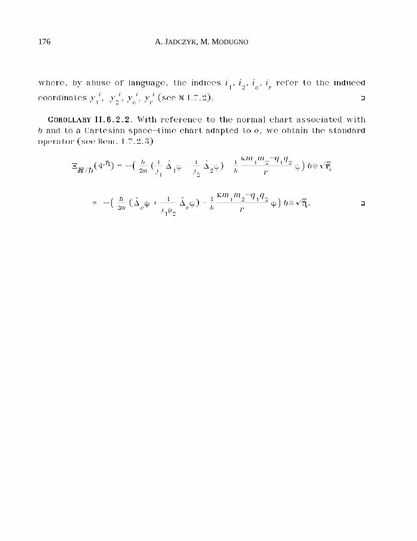
176 A. JADCZYK, M. MODUGNO
where, by abuse of language, the indices i1, i
2, i
c, i
rrefer to the induced
coordinates y1i, y
2i, y
ci, y
ri (see § I.7.2). ò
CCCCOOOORRRROOOOLLLLLLLLAAAARRRRYYYY IIIIIIII....6666....2222....2222. With reference to the normal chart associated withb and to a Cartesian space-time chart adapted to o, we obtain the standardoperator (see Rem. I.7.2.3)
ÚHHHHH/h(„∆∆∆∆∆) = - ⁄ h
2m( 1µ1
êË1¥ _ 1
µ2
êË2¥) _ 1
h
km1m2-q
1q2
r¥^ bæ¢Ã∆∆∆∆∆
= - ⁄ h
2m( êË
c¥ _ 1
µ1µ2
êËr¥) _ 1
h
km1m2-q
1q2
r¥^ bæ¢Ã∆∆∆∆∆. ò
GALILEI GENERAL RELATIVISTIC QUANTUM MECHANICS 177
III - APPENDIX
This appendix is aimed at recalling a few fundamental notions on mani-folds, fibred manifolds, jets, tangent valued forms and general connec-tions, in order to fix our basic terminology and notation.
Some of these ideas and results can be found in any standard book ofdifferential geometry. However, we are concerned with some further geo-metrical techniques, which can be traced only in a more specialised litera-ture. Then, we think that the reader will appreciate a brief sketch; furtherdetails can be found, for instance, in [CCKM], [MM1], [MM2], [Mo2], [Mo3].
The non standard techniques are required by some specific subjects ofour theory, hence cannot be avoided. On the other hand, these techniquesare part of a general approach to differential geometry, which is able torecover in a very compact scheme many standard notions and results. Forthis reason the quick summary below has a certain systematic character.
III.1. Fibred manifolds and bundles
In this section we recall a few basic notions on fibred manifolds. Forfurther details, the reader could refer to [CCKM], [ MM1], [MM2], [Mo2].
Throughout the paper, we deal with smooth manifolds and maps, unless adifferent statement is explicitly mentioned.
III.1.1. Fibred manifolds
Let us start with fibred manifolds and bundles without any additionalstructure.
Let MMMM and NNNN be manifolds.A local map defined on the open subset UUUUçMMMM, is often denoted (by abuse of
178 A. JADCZYK, M. MODUGNO
language) by
f:MMMMéNNNN.
The local maps f:MMMMéNNNN constitute a sheaf
M(MMMM,NNNN) ˆ f:MMMMéNNNN.
In particular, the sheaf of local real valued functions on MMMM is denoted by
F(MMMM) ˆ M(MMMM,·) ˆ f:MMMMé·.
We denote the typical manifold chart of MMMM and NNNN by (x¬) and (yi).
A fibred manifold is defined to be a manifold FFFF together with a surjectivemap of maximum rank
p:FFFFéBBBB.
Let p:FFFFéBBBB be a fibred manifold, with
n ˆ dim BBBB l ˆ dim FFFF - dim BBBB.
The fibre over x is denoted by
FFFFx ˆ p-1(x) ç FFFF.
By the rank theorem, FFFF admits a local fibred splitting in a neighbourhoodof any y$FFFF. Namely, there is an open neighbourhood VVVVçFFFF of y$FFFF, a manifoldFFFFVVVVand a diffeomorphism
È:VVVVép(VVVV)˚FFFFVVVV,
such that
pr1©È = p.
We identify the real functions of FFFF, which are constant along the fibreswith the corresponding functions of BBBB; hence, we have the natural inclusion
F(BBBB) ç F(FFFF).
A fibred chart is defined to be a chart
(x¬,yi) 1≤¬≤n, 1≤i≤l
of FFFF, adapted to a local fibred splitting.
GALILEI GENERAL RELATIVISTIC QUANTUM MECHANICS 179
A section of p:FFFFéBBBB is defined to be a local map
s:BBBBéFFFF,
such that
p©s = idBBBB.
We denote the sheaf of sections of p:FFFFéBBBB by
S(FFFF) ˆ S(FFFFéBBBB) ˆ s:BBBBéFFFF.
We stress that a section s is assumed to be local, i.e. it is defined on anopen subset of the base space; in the particular case when s is defined on thewhole base space, we say that it is global.
L e t FFFF äqEEEEä
pBBBB be a double fibred manifold.
A tube-section is defined to be a section of the type
s : p-1(UUUU) ç EEEE é FFFF
where UUUU ç BBBB is an open subset.The tube sections constitute a sheaf (with respect to the tube-topology)
St(FFFFéEEEEéBBBB) ç S(FFFFéEEEE).
Let p:FFFFéBBBB and q:GGGGéBBBB be fibred manifolds over the same base space.Their fibred product over BBBB is defined to be the fibred manifold
FFFFBBBBGGGG ˆ ø
x$BBBBFFFFx˚GGGG
xé BBBB.
If s$S(GGGGéBBBB), then we denote the pullback of s by
sŸ : FFFF é FFFFBBBBGGGG : f ´ ⁄f, s(p(f))^.
Let p:FFFFéBBBB and q:GGGGéCCCC be fibred manifolds.A fibred morphism is defined to be a pair of local maps
È:FFFFéGGGG È:BBBBéCCCC,
such that
q©È = È©p.
180 A. JADCZYK, M. MODUGNO
Briefly, we say that È is a fibred morphism over È. In particular, if CCCC = BBBBand È = id
BBBB, then we say that È is a fibred morphism over BBBB.
Let p:FFFFéBBBB be a fibred manifold.We say that a local fibred splitting È is a local bundle splitting if it is of
the type
È : VVVV = p-1(UUUU) é UUUU˚FFFFUUUU,
where UUUU = p(VVVV) ç BBBB is an open subset.Then, we say that the fibred manifold p:FFFFéBBBB is a bundle if there exists a
trivialising bundle atlas, i.e. a family of local bundle splittings
Èå:p-1(UUUU
å)éUUUU
å˚FFFF
0å$A
,
where UUUUåå$A
is an open covering of BBBB.
We are concerned with several bundles, whose fibres are smoothly en-dowed with algebraic structures; moreover, we need to prolong this bundlesand their algebraic structures via the tangent and jet functors. This subjectcan be treated in several ways; the most standard approach is based on thetechnique of principal and associated bundles. However, in this report, weprefer to follow a more direct and intrinsic way, which is very suitable forour goals and fits the intrinsic spirit of our viewpoint. Here and in the fol-lowing sections, we just sketch the main ideas and results; for a more gen-eral and detailed treatment the reader can refer to [CCKM].
III.1.2. Structured bundles
Next, we consider bundles whose fibres are equipped with an algebraicstructure.
A vector bundle is defined to be a bundle p:FFFFéBBBB smoothly equipped with avector structure on its fibres. Thus, by definition, each fibre FFFF
xis a vector
space; moreover, there exists a trivialising bundle atlas, whose type-fibre FFFF0
is a vector space, such that the maps Èåx:FFFFxéFFFF
0, with x$UUUU
å, å$A, are linear.
A fibred morphism between vector bundles is said to be linear if it yieldslinear maps between the fibres.
If p:FFFFéBBBB is a vector bundle, then we obtain the global section and the fi-
GALILEI GENERAL RELATIVISTIC QUANTUM MECHANICS 181
bred morphisms over BBBB
0:BBBBéFFFF _:FFFFBBBBFFFFéFFFF ÷:·˚FFFFéFFFF,
which fulfill the standard algebraic properties and characterise the vectorstructure of the bundle.
An affine bundle is defined to be a bundle p:FFFFéBBBB smoothly equipped withan affine structure on its fibres. Thus, by definition, each fibre FFFF
xis an
affine space associated with a vector space ÃFFFFx; moreover, there exists a
trivialising bundle atlas, whose type-fibre FFFF0is an affine space associated
with a vector space ÃFFFF0, such that the maps È
åx:FFFF
xéFFFF
0, with x$UUUU
å, å$A, are
affine.It can be proved that
ÃFFFF ˆ øx$BBBB
ÃFFFFxé BBBB
has a natural structure of vector bundle; this is said to be the vector bundleassociated with the affine bundle.
A fibred morphism between affine bundles is said to be affine if it yieldsaffine maps between the fibres.
If p:FFFFéBBBB is an affine bundle, then we obtain the fibred morphism over BBBB
_:FFFFBBBBÃFFFFéFFFF,
which fulfills the standard algebraic properties and characterises the affinestructure of the bundle.
Other algebraic structures on bundles can be defined in this way. For in-stance, the complex structure can be defined by considering a linear endo-
morphism ˘, such that ˘2 = -1.
III.1.3. Positive semi-vector bundles
Furthermore, in order to describe rigorously the units of measurementand to introduce the bundles of densities, we need the notions of a positivesemi-vector space and a positive semi-vector bundle.
Let us consider ·_ ˆ x$· ¡ x>0 as a semi-field, i.e. as an abelian semi-group with respect to the addition and a group with respect to the multipli-
182 A. JADCZYK, M. MODUGNO
cation.Then, we define a semi-vector space to be an abelian semi-group UUUU with a
scalar multiplication by ·_, which fulfills the standard properties
(r _ s) u = r u _ s u (r s) u = r (s u)
r (u _ v) = r u _ r v 1 u = u År,s$·_, u,v$UUUU.
A vector space VVVV and a basis B yield a semi-vector space in a natural way.
In fact, the subset finitely generated by B over ·_ turns out to be a semi-
vector space. In particular, ·_n, with n≥1, is a semi-vector space.Moreover, any vector space VVVV can be regarded as a semi-vector space in a
natural way. On the other hand, a semi-vector space UUUU is said to be a posi-tive semi-vector space if the scalar multiplication cannot be extended nei-
ther to ·_‰0, nor to ·. Hence, a positive semi-vector space contains nei-ther the zero element, nor the negative of any element. Thus, a semi-vectorspace is a vector space, or a positive semi-vector space, or a positive semi-vector space extended by the zero element.
Several concepts and results of standard linear and multi-linear algebrarelated to vector spaces (including linear and multi-linear maps, bases, di-mension, tensor products and duality) can be easily repeated for semi- vec-tor spaces and positive semi-vector spaces. The main caution to be taken isto avoid the formulations which involve the zero element. We shall use forsemi-vector spaces the standard terminology used for vector spaces.
Let UUUU be a semi-vector space and VVVV a vector space. By regarding VVVV as a
semi-vector space, we can consider the tensor product over ·_
UUUUÆVVVV.
We observe that the semi-vector space UUUUÆVVVV turns out to be also a vectorspace, according to the formula
·˚(UUUUÆVVVV) é UUUUÆVVVV : (r, uæv) ´ uæ(rv).
So, any positive semi-vector space UUUU can be extended to the vector spaceUUUUÆ·, through the natural inclusion UUUU ç UUUUÆ·.
In particular, we are concerned with 1-dimensional positive semi-vector
GALILEI GENERAL RELATIVISTIC QUANTUM MECHANICS 183
spaces.
If VVVV is an oriented 1-dimensional vector space, then the positively oriented
subset VVVV_ ç VVVV is a positive space.Moreover, if WWWW is a further vector space, then we obtain the following
useful canonical isomorphisms25
VVVV_ÆWWWW ≠ VVVVÆWWWW
and, in particular,
VVVV_Æ· ≠ VVVVÆ· ≠ VVVV.
Let UUUU and VVVV be 1-dimensional positive semi-vector spaces.In order to write formulas in a way apparently equal to the standard one
used by physicists, it is convenient to treat the elements of 1-dimensionalpositive spaces as they were numbers and introduce some conventions.
So, we can treat the dual element ¨$UUUU* of u$UUUU as its “inverse” and write
UUUU-1 ˆ UUUU* ¨ =1u.
Moreover, if u$UUUU and v$VVVV, then we often omit the tensor product æ andjust write
u v ˆ uæv.
Furthermore, we make the canonical identification
UUUUÆUUUU* ≠ ·_.
Let UUUU be a 1-dimensional positive semi-vector space.A square root of UUUU is defined to be a 1-dimensional positive semi-vector
space ¢ÃÃUUUU together with a quadratic map q:¢ÃÃUUUU éUUUU, such that, for each 1-dimensional positive semi-vector space ¢ÃÃUUUU ' and each quadratic mapq':¢ÃÃUUUU 'éUUUU, there is a unique linear map l:¢ÃÃUUUU é¢ÃÃUUUU ', which yields q'©l = q.
By a standard argument related to universal properties, the square root isunique up to a canonical isomorphism. Moreover, we can easily prove the ex-
25 The first tensor product is taken over ·_ and the second one over ·.
184 A. JADCZYK, M. MODUGNO
istence of a square root. So, in the following, we shall refer to “the” squareroot ¢ÃÃUUUU of UUUU.
The universal property implies that the quadratic map q is a bijection. So,we obtain the inverse bijection ¢:UUUUé¢ÃÃUUUU :u´¢Ãu.
Moreover, the universal property of the tensor product implies that thereis a unique linear isomorphism i:¢ÃÃUUUU Æ¢ÃÃUUUU éUUUU, which yields i©∂ = q, where∂:¢ÃÃUUUU é¢ÃÃUUUU Æ¢ÃÃUUUU is the canonical map.
In an analogous way, for every natural number q, we can define the q-rootUUUU1/q of UUUU.
Therefore, for every pair of natural numbers p and q, we write
UUUUp/q ˆ UUUU1/qÆ …p times
ÆUUUU1/q UUUU0 ˆ · UUUU- p/q ˆ UUUU*1/qÆ …p times
ÆUUUU*1/q.
If VVVV is an oriented 1-dimensional vector space, then we set ¢ÃÃVVVV ˆ ÊÕVVVV_.In particular, if WWWW is an oriented n-dimensional vector space, then we ob-
tain the square root positive semi-vector space ÊôÕÓnWWWW.
The above algebraic constructions on positive semi-vector spaces can beeasily extended to bundles.
So, a semi-vector bundle and a positive semi-vector bundle can be de-fined analogously to a vector bundle. Moreover, if p:FFFFéBBBB is a 1-dimensionaloriented vector bundle, then we obtain in a natural way the positive semi-
vector bundle p:¢ÃÃFFFF éBBBB and the canonical fibred isomorphism ¢ÃÃFFFF ÆBBBB¢ÃÃFFFF ≠ FFFF_
over BBBB.We observe that these constructions lead naturally to a generalisation of
the half-densities due to de Rham (see [dR]).
III.2. Tangent prolongation of fibred manifolds
In this section we recall a few basic notions on the tangent prolongationof fibred manifolds. For further details, the reader could refer to [CCKM],[ MM1], [MM2], [Mo2].
III.2.1 Tangent prolongation of manifolds
We start by considering just simple manifolds.
We denote the tangent functor from the category of manifolds to the cat-
GALILEI GENERAL RELATIVISTIC QUANTUM MECHANICS 185
egory of vector bundles by T.So, if MMMM is a manifold, then we have the vector bundle
πMMMM:TMMMMéMMMM
and if f$M(MMMM,NNNN), then we have the linear fibred morphism over f
Tf:TMMMMéTNNNN,
or, equivalently, the section
df : MMMM é T*MMMM ÆMMMM˚NNNN
TNNNN : x ´ Txf.
We set
T(MMMM) ˆ S(TMMMMéMMMM) T*(MMMM) ˆ S(T*MMMMéMMMM).
We denote the induced linear fibred charts of TMMMM and T*MMMM by
(x¬, îx¬) (x¬, îx¬)
and the induced bases of T(MMMM) and T*(MMMM) by
(Ù¬) ˆ (Ùx
¬) (d¬) ˆ (dx¬).
Then, we obtain the coordinate expressions
(yi, îyi)©Tf = (fi, Ù¬fi îx¬) df = Ù
¬fi d¬æ(Ù
i©f).
If c:·éMMMM is a local map, then we set
dc : · é TMMMM : ¬ ´ Tc(¬,1).
If c:·˚MMMMéNNNN is a map defined in a neighbourhood of 0˚MMMM ç ·˚MMMM, then weset
Ùc : MMMM é TNNNN : x ´ d(cx)(0).
III.2.1 Tangent prolongation of fibred manifolds
Next, we consider fibred manifolds.
Let p:FFFFéBBBB be a fibred manifold.We have the vector bundle
186 A. JADCZYK, M. MODUGNO
πFFFF:TFFFFéFFFF
and the fibred manifold
Tp:TFFFFéTBBBB.
If p:FFFFéBBBB is a bundle, then also Tp:TFFFFéTBBBB is a bundle.The induced fibred chart of TFFFF is
(x¬, yi, îx¬, îyi).
A vector field X$T(FFFF) is said to be projectable if it projects over a vectorfield X$T(BBBB). The coordinate expression of a projectable vector field is ofthe type
X = Xµ Ùµ_ Xi Ù
iXµ$F(BBBB), Xi$F(FFFF).
The projectable vector fields constitute the subsheaf
P(FFFF) ç T(FFFF).
We denote the vertical functor from the category of fibred manifolds tothe category of vector bundles by V.
So, if p:FFFFéBBBB is a fibred manifold, then we have the vertical subbundle overFFFF
VFFFF ˆ kerFFFFTp ç TFFFF,
and the exact sequence of vector bundles over FFFF
0 ä V FFFFä T FFFF äBBBBT BBBB ä0.
The induced fibred chart of VFFFF is
(x¬, yi, îyi).
A vector field X$T(FFFF) is said to be vertical if it is vertical valued, i.e. ifit projects over a zero vector field X$T(BBBB). The coordinate expression of avertical vector field is of the type
X = Xi Ùi
Xi$F(FFFF).
The vertical vector fields constitute the subsheaf
GALILEI GENERAL RELATIVISTIC QUANTUM MECHANICS 187
V(FFFF) ç P(FFFF) ç T(FFFF).
If p:FFFFéBBBB is a vector bundle, then the tangent prolongation of the distin-guished section and fibred morphisms
T0:TBBBBéTFFFF T_:TFFFFTBBBBTFFFFéTFFFF T÷:·˚TFFFFéTFFFF
makes
Tp:TFFFFéTBBBB
a vector bundle.
If p:FFFFéBBBB is an affine bundle associated with the vector bundle, ãp:ÃFFFFéBBBB,then the tangent prolongation of the distinguished fibred morphism
T_:TFFFFTBBBBTÃFFFFéTFFFF
makes
Tp:TFFFFéTBBBB
an affine bundle associated with the vector bundle
Tãp:TÃFFFFéTBBBB.
The tangent prolongation of other algebraic structures on bundles can beobtained in this way. For instance, the complex structure can be prolonged by
considering the linear endomorphism T˘, which fulfills (T˘)2 = -1.In fact, the algebraic constructions of previous sections concerning posi-
tive semi-vector spaces and positive spaces can be easily extended in asmooth way to any vector bundle (see [CCKM]).
The tangent prolongation and the related differential operators extend tosemi-vector and positive bundles in a natural way. Here, we add a few obser-vations, which are useful for a clear understanding of our procedures.
The tangent space of a positive space UUUU turns out to be TUUUU = UUUU˚(·æUUUU).Hence, the vertical bundle of a positive bundle UUUUéBBBB turns out to be the
vector bundle VUUUU = UUUUBBBB(·æUUUU).
The differential operations such as exterior differential, covariant differ-ential, Lie derivative and so on, commute with the tensor product with a
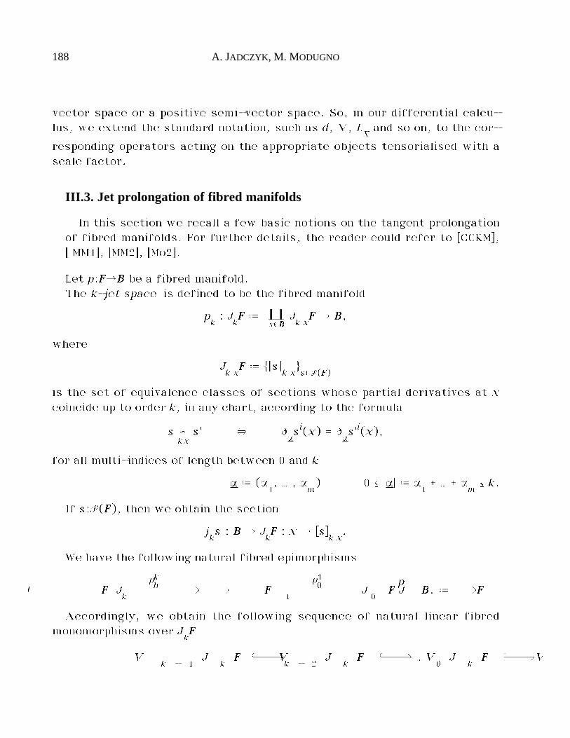
188 A. JADCZYK, M. MODUGNO
vector space or a positive semi-vector space. So, in our differential calcu-lus, we extend the standard notation, such as d, ı, L
Xand so on, to the cor-
responding operators acting on the appropriate objects tensorialised with ascale factor.
III.3. Jet prolongation of fibred manifolds
In this section we recall a few basic notions on the tangent prolongationof fibred manifolds. For further details, the reader could refer to [CCKM],[ MM1], [MM2], [Mo2].
Let p:FFFFéBBBB be a fibred manifold.The k-jet space is defined to be the fibred manifold
pk: J
kFFFF ˆ ø
x$BBBBJk xFFFF é BBBB,
where
Jk xFFFF ˆ [s]
k xs$S(FFFF)
is the set of equivalence classes of sections whose partial derivatives at xcoincide up to order k, in any chart, according to the formula
s –kxs' ∞ Ù
åsi(x) = Ù
ås'i(x),
for all multi-indices of length between 0 and k
å ˆ (å1, … , å
m) 0 ≤ ¡å¡ ˆ å
1_ … _ å
m≤ k.
If s:S(FFFF), then we obtain the section
jks : BBBB é J
kFFFF : x ´ [s]
k x.
We have the following natural fibred epimorphisms
Jk
FFFF äpkhJ ä J
1FFFF ä
p10 J
0FFFF ˆ FFFFäp
BBBB.
Accordingly, we obtain the following sequence of natural linear fibredmonomorphisms over J
kFFFF
Vk - 1
JkFFFF ‹V
k - 2J
kFFFF ‹… V
0J
kFFFF ‹V
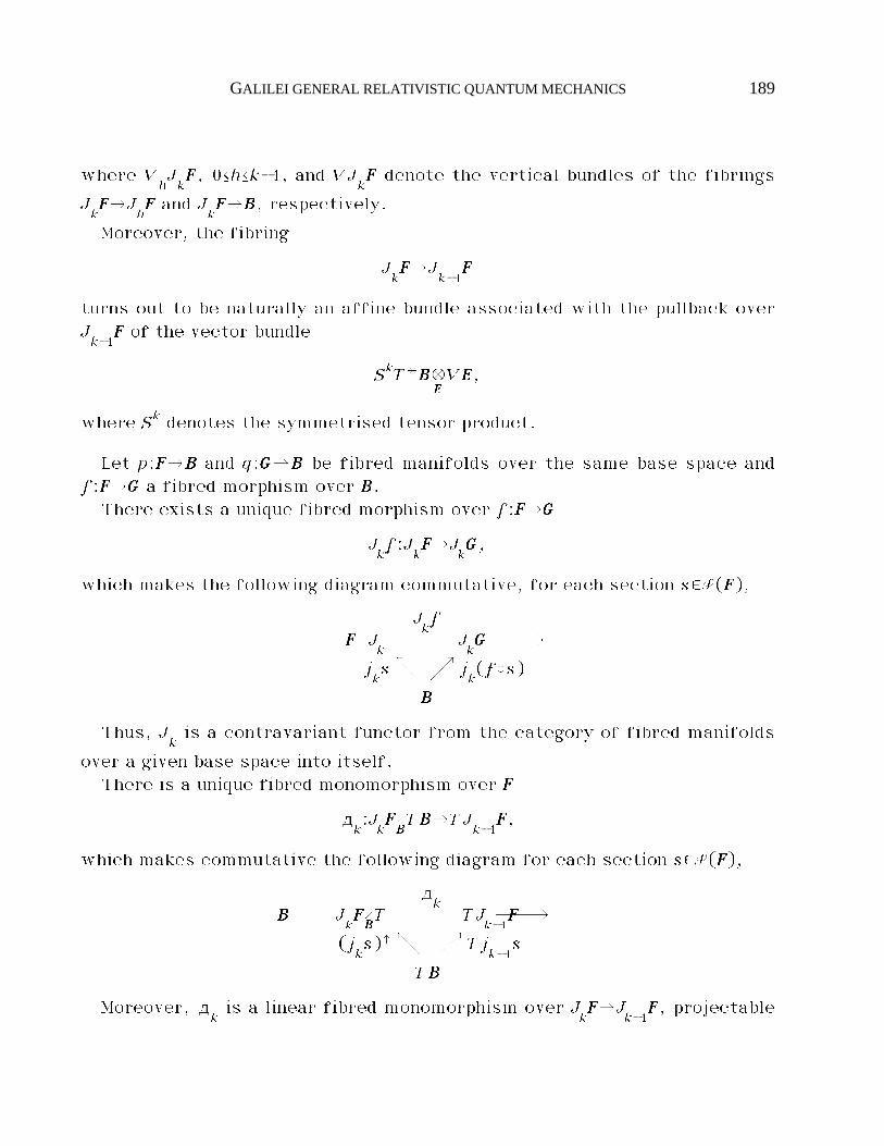
GALILEI GENERAL RELATIVISTIC QUANTUM MECHANICS 189
where VhJkFFFF, 0≤h≤k-1, and VJ
kFFFF denote the vertical bundles of the fibrings
JkFFFFéJ
hFFFF and J
kFFFFéBBBB, respectively.
Moreover, the fibring
JkFFFFéJ
k-1FFFF
turns out to be naturally an affine bundle associated with the pullback overJk-1FFFF of the vector bundle
SkT*BBBBÆEEEEVEEEE,
where Sk denotes the symmetrised tensor product.
Let p:FFFFéBBBB and q:GGGGéBBBB be fibred manifolds over the same base space andf:FFFFéGGGG a fibred morphism over BBBB.
There exists a unique fibred morphism over f:FFFFéGGGG
Jkf:J
kFFFFéJ
kGGGG,
which makes the following diagram commutative, for each section s$S(FFFF),
Jk
FFFF äJkf
JkGGGG
jks Ü Ö j
k(f©s)
BBBB
Thus, Jkis a contravariant functor from the category of fibred manifolds
over a given base space into itself.There is a unique fibred monomorphism over FFFF
dk:JkFFFFBBBBTBBBBéTJ
k-1FFFF,
which makes commutative the following diagram for each section s$S(FFFF),
JkFFFFBBBBTBBBB ä
dk
TJk-1FFFF
(jks)Ÿ Ü Ö Tj
k-1s
TBBBB
Moreover, dkis a linear fibred monomorphism over J
kFFFFéJ
k-1FFFF, projectable
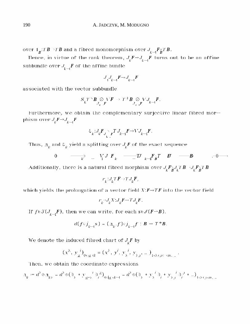
190 A. JADCZYK, M. MODUGNO
over 1BBBB:TBBBBéTBBBB and a fibred monomorphism over J
k-1FFFFBBBBTBBBB.
Hence, in virtue of the rank theorem, JkFFFFéJ
k-1FFFF turns out to be an affine
subbundle over Jk-1FFFF of the affine bundle
J1Jk-1FFFFéJ
k-1FFFF
associated with the vector subbundle
SkT*BBBB Æ
Jk-1FFFFVFFFF é T*BBBB Æ
Jk-1FFFFVJ
k-1FFFF.
Furthermore, we obtain the complementary surjective linear fibred mor-phism over J
kFFFFéJ
k-1FFFF
ªk:JkFFFF ˚Jk-1FFFFTJ
k-1FFFFéVJ
k-1FFFF.
Thus, dkand ª
kyield a splitting over J
kFFFF of the exact sequence
0 ä VJk - 1
FFFF äTJk - 1
FFFF äJk-1FFFFBBBBT BBBB ä0.
Additionally, there is a natural fibred morphism over JkFFFFBBBBJkTBBBBéJ
kFFFFBBBBTBBBB
rk:JkTFFFFéTJ
kFFFF,
which yields the prolongation of a vector field X:FFFFéTFFFF into the vector field
rk©J
kX:J
kFFFFéTJ
kFFFF.
If f$F(Jk-1FFFF), then we can write, for each s$S(FFFFéBBBB),
d(f©jk-1s) = (d
k.f)©j
k-1f : BBBB é T*BBBB.
We denote the induced fibred chart of JkFFFF by
(x¬, yåi)0≤¡å¡≤k
= (x¬, yi, y¬i, y
¬µ, … )
1≤¬≤µ≤…≤m, ….
Then, we obtain the coordinate expressions
dkˆ d¬æd
k¬= d¬æ(Ù
¬_ y
å_¬i Ù
iå)0≤¡å¡≤k-1
= d¬æ(Ù¬_ y
¬i Ù
i_ y
¬µi Ù
iµ _ …)
1≤¬≤µ≤m, …
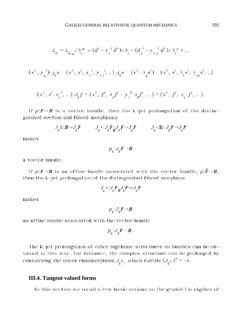
GALILEI GENERAL RELATIVISTIC QUANTUM MECHANICS 191
ªkˆ ª
k åæÙ
iå = (di - y
¬i d¬)æÙ
i_ (d
µi - y
¬µi d¬)æÙ
iµ _ ….
(x¬, yåi)©j
ks = (x¬, yi, y
¬i, y
¬µi, …)©j
ks = (x¬, Ù
åsi) = (x¬, si, Ù
¬si, Ù
¬µsi, …)
(x¬, zi, z¬i, … )©J
kf = (x¬, fi, Ù
¬fi _ y
¬h Ù
hfi, … ) = (x¬, fi, d
¬.fi, … ).
If p:FFFFéBBBB is a vector bundle, then the k-jet prolongation of the distin-guished section and fibred morphisms
Jk0:BBBBéJ
kFFFF J
k_:J
kFFFFBBBBJkFFFFéJ
kFFFF J
k÷:·˚J
kFFFFéJ
kFFFF
makes
pk:JkFFFFéBBBB
a vector bundle.
If p:FFFFéBBBB is an affine bundle associated with the vector bundle, ãp:ÃFFFFéBBBB,then the k-jet prolongation of the distinguished fibred morphism
Jk_:J
kFFFFBBBBJkÃFFFFéJ
kFFFF
makes
pk:JkFFFFéBBBB
an affine bundle associated with the vector bundle
pk:JkÃFFFFéBBBB.
The k-jet prolongation of other algebraic structures on bundles can be ob-tained in this way. For instance, the complex structure can be prolonged by
considering the linear endomorphism Jk˘, which fulfills (J
k˘)2 = -1.
III.4. Tangent valued forms
In this section we recall a few basic notions on the graded Lie algebra of
192 A. JADCZYK, M. MODUGNO
tangent valued forms. For further details, the reader could refer to [ MM].
First, let us consider just a manifold, MMMM.A tangent valued form of MMMM is defined to be a section
ƒ:MMMMéLT*MMMMÆMMMMTMMMM.
We have the coordinate expression
ƒ = ƒ¬1…¬r
µ d¬1◊…◊d¬ræÙµ
ƒ¬1…¬r
µ$F(MMMM).
In particular, the vector fields are tangent valued forms of degree 0.The Lie bracket of vector fields can be naturally extended to a graded Lie
bracket of tangent valued forms, which is called the Frölicher-Nijenhuisbracket .
Namely, there is a unique sheaf morphism
[,] : LrT*(MMMM) Æ
F(MMMM)T(MMMM) ˚ L
sT*(MMMM) Æ
F(MMMM)T(MMMM) é L
r_sT*(MMMM) Æ
F(MMMM)T(MMMM)
which on decomposable forms is given by
[åæu, ∫æv] = å◊∫æ[u, v] _
_å◊Lu∫æv - (-1)¡å¡¡∫¡∫◊L
våæu _ (-1)ri
vå◊d∫æu - (-1)¡å¡¡∫¡_¡∫¡ i
u∫◊dåæv.
We have the coordinate expression
[ƒ, ¥] = (ƒ®¬1…¬r
Ù®¥µ
¬r_1…¬r_s
- (-1)rs ¥®¬1…¬s
Ù®ƒµ
¬s_1…¬r_s_
- r ƒµ¬1…¬r-1
® Ù¬r¥®
¬r_1…¬r_s
_ (-1)rs s ¥µ¬1…¬s-1
® Ù¬sƒ®
¬s_1…¬r_s
)÷d¬1◊…◊d¬r_sæÙµ.
Thus, LT*(MMMM) ÆF(MMMM)
T(MMMM), together with the F-N bracket, is a sheaf of
graded Lie algebras, namely we have
[ƒ _ ƒ', ¥] = [ƒ, ¥] _ [ƒ', ¥] [ƒ, ¥ _ ¥'] = [ƒ, ¥] _ [ƒ, ¥']
[k ƒ, ¥] = k [ƒ, ¥] = [ƒ, k ¥]
[ƒ, ¥] = - (-1)¡ƒ¡¡¥¡ [¥, ƒ]
GALILEI GENERAL RELATIVISTIC QUANTUM MECHANICS 193
[ª, [ƒ, ¥]] = [[ª, ƒ], ¥] _ (-1)¡ª¡¡ƒ¡ [ƒ, [ª, ¥]]
ƒ, ¥, ª$LT*(MMMM) ÆF(MMMM)
T(MMMM); k$·.
Now, let us replace the manifold MMMM with the fibred manifold p:FFFFéBBBB andconsider the sheaf of tangent valued forms of FFFF
LT*(FFFF) ÆF(FFFF)
T(FFFF).
A tangent valued form
ƒ:FFFFéLT*BBBBÆFFFFTFFFF,
is said to be projectable if it projects over a tangent valued form of BBBB
ƒ:BBBBéLT*BBBBÆBBBBTBBBB.
The projectable tangent valued forms constitute the subsheaf
LT*(BBBB) ÆF(BBBB)
P(FFFF) ç LT*(BBBB) ÆF(BBBB)
T(FFFF).
Their coordinate expression is of the type
ƒ = (ƒ¬1…¬r
µ Ùµ_ ƒ
¬1…¬r
i Ùi^æd¬1◊…◊d¬r
with
ƒ¬1…¬r
µ $ F(BBBB) ƒ¬1…¬r
i $ F(FFFF).
As a special case, we have the vertical valued forms
ƒ:FFFFéLT*BBBBÆFFFFVFFFF,
which project over the zero tangent valued form of B
ƒ = 0 : BBBB é LT*BBBBÆBBBBTBBBB.
The vertical valued forms constitute the subsheaf
LT*(BBBB) ÆF(BBBB)
V(FFFF) ç LT*(BBBB) ÆF(BBBB)
P(FFFF).
194 A. JADCZYK, M. MODUGNO
Their coordinate expression is of the type
ƒ = ƒ¬1…¬r
i Ùiæd¬1◊…◊d¬r.
The projectable tangent valued forms constitute a subalgebra of the alge-bra of tangent valued forms. Moreover, we have
[ƒ,¥]á
= [ƒ , ¥ ] ƒ, ¥$LT*(BBBB) ÆF(BBBB)
P(FFFF).
Let p:FFFFéBBBB be a vector bundle. A projectable tangent valued form
ƒ:FFFFéLT*BBBBÆFFFFTFFFF
is said to be linear if it is a linear fibred morphism over ƒ.The coordinate expression of a linear projectable tangent valued form is of
the type
ƒ = (ƒ¬1…¬r
µ Ùµ_ ƒ
¬1…¬r
ijyj Ù
i^æd¬1◊…◊d¬r
with
ƒ¬1…¬r
µ, ƒ¬1…¬r
ij$ F(BBBB).
The linear projectable tangent valued forms constitute a subalgebra of thealgebra of projectable tangent valued forms.
Let p:FFFFéBBBB be an affine bundle. A projectable tangent valued form
ƒ:FFFFéLT*BBBBÆFFFFTFFFF
is said to be affine if it is an affine fibred morphism over ƒ.The coordinate expression of an affine projectable tangent valued form is
of the type
ƒ = ⁄ƒ¬1…¬r
µ Ùµ_ (ƒ
¬1…¬r
ijyj _ ƒ
¬1…¬r
i©) Ù
i^æd¬1◊…◊d¬r
with
ƒ¬1…¬r
µ, ƒ¬1…¬r
ij, ƒ
¬1…¬r
i©$ F(BBBB).
The affine projectable tangent valued forms constitute a subalgebra of the
GALILEI GENERAL RELATIVISTIC QUANTUM MECHANICS 195
algebra of projectable tangent valued forms.
III.5. General connections
In this section we recall a few basic notions on general connections. Forfurther details, the reader can refer to [ MM].
Let p:FFFFéBBBB be a fibred manifold.
A connection is defined to be a section
c:FFFFéJ1FFFF,
i.e. a tangent valued 1-form
c:FFFFéT*BBBBÆFFFFTFFFF,
which projects onto
cˆ1BBBB:BBBBéT*BBBBÆ
BBBBTBBBB,
i.e. a linear fibred morphism over FFFF
c:FFFFFFFFTBBBBéTFFFF,
which projects onto
cˆ1BBBB:TBBBBéTBBBB.
Its coordinate expression is of the type
(x¬, yi, y¬i)©c = (x¬, yi, c
¬i),
i.e.
c = d¬æ(Ù¬_ c
¬iæÙ
i) c
¬i$F(FFFF).
A connection c yields the linear fibred epimorphism over FFFF
~c:TFFFFéVFFFF,
with coordinate expressions
~c= (di - c
¬i d¬)æÙ
i,
196 A. JADCZYK, M. MODUGNO
and the translation fibred isomorphism over FFFF
ıc:J1FFFFéT*BBBBÆ
FFFFVFFFF,
with coordinate expression
ıc= (y
¬i - c
¬i) d¬æÙ
i.
The maps ~cand ı
ccharacterise the connection c itself.
The covariant differential of a section s$S(FFFF) is defined to be the section
ıcs ˆ ı
c©j
1s : BBBB é T*BBBBÆ
FFFFVFFFF,
with coordinate expression
ıcs = (Ù
¬si - c
¬i©s) d¬æ(Ù
i©s).
The covariant differential of a tangent valued form ƒ$LrT*(FFFF) Æ
F(FFFF)T(FFFF) is
defined to be the tangent valued form
dcƒ ˆ [c,ƒ] : FFFFéL
r_1T*FFFFÆ
FFFFTFFFF.
In particular, if ƒ is projectable, then its covariant differential turns outto be vertical valued
dcƒ ˆ [c,ƒ] : FFFFéL
r_1T*BBBBÆ
FFFFVFFFF
and its coordinate expression is
dcƒ = (- Ù
¬1ƒ¬2…¬r_1
µ cµi - Ù
µc¬1
i ƒ¬2…¬r_1
µ _
_ Ù¬1ƒ¬2…¬r_1
i _ c¬1
j Ùjƒ¬2…¬r_1
i - Ùjc¬1
i ƒ¬2…¬r_1
j) d¬1◊…◊d¬r_1æÙi.
For each ƒ,¥$LrT*(FFFF) Æ
F(FFFF)T(FFFF), we have the following properties
dc(ƒ _ ¥) = d
cƒ _ d
c¥
dc[ƒ, ¥] = [d
cƒ, ¥] _ (-1)¡ƒ¡ [ƒ, d
c¥]
GALILEI GENERAL RELATIVISTIC QUANTUM MECHANICS 197
dc(∑◊ƒ) = d∑◊~
c(ƒ) _ (-1)¡∑¡ ∑◊d
cƒ ∑$T*(BBBB)
and, if ƒ is a projectable vector field
⁄dc(ƒ)^(u) = [c(u), ƒ] - c([u,ƒ]), Åu$T(BBBB).
The curvature of c is defined to be the vertical valued 2-form
Rcˆ 1
2dcc : FFFF é L
2T*BBBBÆ
FFFFVFFFF,
with coordinate expression
Rc= (Ù
¬cµi _ c
¬j Ù
jcµi) d¬◊dµæÙ
i.
The curvature is characterised by the following property
2 Rc(X,Y) = [c(X),c(Y)] - c([X,Y]) X,Y$T(BBBB).
We have the Bianchi identity
dc2ƒ = [R
c,ƒ] ƒ$LT*(FFFF) Æ
F(FFFF)T(FFFF).
In particular, we obtain
dcRc= 0,
in virtue of
[c,Rc] = d
cRcˆ 1
2dc2c = 1
2[Rc,c].
Moreover, if
ƒ ˆ c(ƒ) : BBBB é LT*BBBBÆFFFFTFFFF
is a horizontal tangent valued form, then we obtain the formula26
dcƒ = - R
c◊ƒ,
with coordinate expression
26 Here ◊ denotes the exterior product combined with an interior product.
198 A. JADCZYK, M. MODUGNO
dcƒ = - 2 R
c µ¬1
i ƒ¬2…¬r_1
µ Ùiæd¬1◊…◊d¬r_1.
Given a section ß:FFFFéT*BBBBÆFFFFVFFFF, the torsion of c is defined to be the 2-form
†cˆ d
cß : FFFF é L
2T*BBBBÆ
FFFFVFFFF.
We have the Bianchi identity
dc†c= [R
c, ß].
Let FFFFéBBBB be a vector bundle. A connection c is said to be linear if, as a fi-bred morphism c:FFFFéJ
1FFFF over BBBB, it is linear. A connection is linear if and only
if, in a linear fibred chart, its coordinate expression is of the following type
c¬i = c
¬ijyj c
¬ij$F(BBBB).
The covariant differential of a linear projectable tangent valued form withrespect to a linear connection turns out to be a linear vertical valued form.
Let FFFFéBBBB be an affine bundle. A connection c is said to be affine if, as afibred morphism c:FFFFéJ
1FFFF over BBBB, it is affine. A connection is affine if and
only if, in an affine fibred chart, its coordinate expression is of the followingtype
c¬i = c
¬ijyj _ c
¬i©
c¬ij, c
¬i©$F(BBBB).
The covariant differential of an affine projectable tangent valued formwith respect to an affine connection turns out to be an affine vertical valuedform.
Connections adapted to other algebraic structures on bundles can be ob-tained in a similar way. For instance, a complex connection can be defined asa real linear fibred morphism c:FFFFéJ
1FFFF over BBBB, which makes the following di-
agram commute
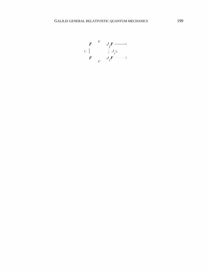
GALILEI GENERAL RELATIVISTIC QUANTUM MECHANICS 199
FFFF äc
J1FFFF
˘ ï ï J1˘
FFFF äc
J1FFFF
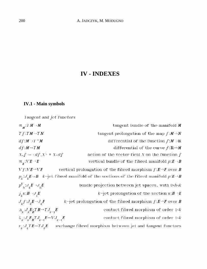
200 A. JADCZYK, M. MODUGNO
IV - INDEXES
IV.1 - Main symbols
Tangent and jet functors
πMMMM:TMMMMéMMMM tangent bundle of the manifold MMMM
Tf:TMMMMéTNNNN tangent prolongation of the map f:MMMMéNNNN
df:MMMMéT*MMMM differential of the function f:MMMMé·
df:MMMMéTMMMM differential of the curve f:·éMMMM
X.f ˆ Çdf,X¶ + Xœdf action of the vector field X on the function f
πEEEE:VEEEEéEEEE vertical bundle of the fibred manifold p:EEEEéBBBB
Vf:VEEEEéVFFFF vertical prolongation of the fibred morphism f:EEEEéFFFF over BBBB
pk:JkEEEEéBBBB k-jet fibred manifold of the sections of the fibred manifold p:EEEEéBBBB
pkh:JkEEEEéJ
hEEEE bundle projection between jet spaces, with 0≤h<k
jks:BBBBéJ
1EEEE k-jet prolongation of the section s:BBBBéEEEE
Jkf:J
kEEEEéJ
kFFFF k-jet prolongation of the fibred morphism f:EEEEéFFFF over BBBB
dk:JkEEEEBBBBTBBBBéTJ
k-1EEEE contact fibred morphism of order 1≤k
ªk:JkEEEEBBBBTJ
k-1EEEEéVJ
k-1EEEE contact fibred morphism of order 1≤k
rk:JkTEEEEéTJ
kEEEE exchange fibred morphism between jet and tangent functors
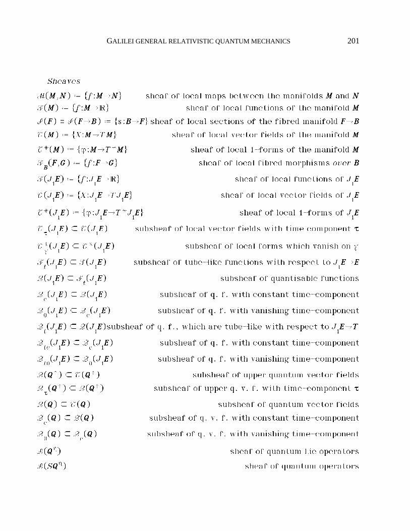
GALILEI GENERAL RELATIVISTIC QUANTUM MECHANICS 201
Sheaves
M(MMMM,NNNN) ˆ f:MMMMéNNNN sheaf of local maps between the manifolds MMMM and NNNNF(MMMM) ˆ f:MMMMé· sheaf of local functions of the manifold MMMM
S(FFFF) + S(FFFFéBBBB) ˆ s:BBBBéFFFF sheaf of local sections of the fibred manifold FFFFéBBBB
T(MMMM) ˆ X:MMMMéTMMMM sheaf of local vector fields of the manifold MMMM
T*(MMMM) ˆ ƒ:MMMMéT*MMMM sheaf of local 1-forms of the manifold MMMM
FBBBB(FFFF,GGGG) ˆ f:FFFFéGGGG sheaf of local fibred morphisms over BBBB
F(J1EEEE) ˆ f:J
1EEEEé· sheaf of local functions of J
1EEEE
T(J1EEEE) ˆ X:J
1EEEEéTJ
1EEEE sheaf of local vector fields of J
1EEEE
T*(J1EEEE) ˆ ƒ:J
1EEEEéT*J
1EEEE sheaf of local 1-forms of J
1EEEE
T††††(J1EEEE) ç T(J
1EEEE) subsheaf of local vector fields with time component ††††
T*˙(J1EEEE) ç T*(J
1EEEE) subsheaf of local forms which vanish on ˙
Ft(J1EEEE) ç F(J
1EEEE) subsheaf of tube-like functions with respect to J
1EEEEéEEEE
Q(J1EEEE) ç F
t(J1EEEE) subsheaf of quantisable functions
Qc(J1EEEE) ç Q(J
1EEEE) subsheaf of q. f. with constant time-component
Q0(J1EEEE) ç Q
c(J1EEEE) subsheaf of q. f. with vanishing time-component
Qt(J1EEEE) ç Q(J
1EEEE)subsheaf of q. f., which are tube-like with respect to J
1EEEEéTTTT
Qtc(J1EEEE) ç Q
c(J1EEEE) subsheaf of q. f. with constant time-component
Qt0(J1EEEE) ç Q
0(J1EEEE) subsheaf of q. f. with vanishing time-component
Q(QQQQŸ) ç T(QQQQŸ) subsheaf of upper quantum vector fields
Q††††(QQQQŸ) ç Q(QQQQŸ) subsheaf of upper q. v. f. with time-component ††††
Q(QQQQ) ç T(QQQQ) subsheaf of quantum vector fields
Qc(QQQQ) ç Q(QQQQ) subsheaf of q. v. f. with constant time-component
Q0(QQQQ) ç Q
c(QQQQ) subsheaf of q. v. f. with vanishing time-component
L(QQQQ∆) sheaf of quantum Lie operators
L(SQQQQ∆) sheaf of quantum operators
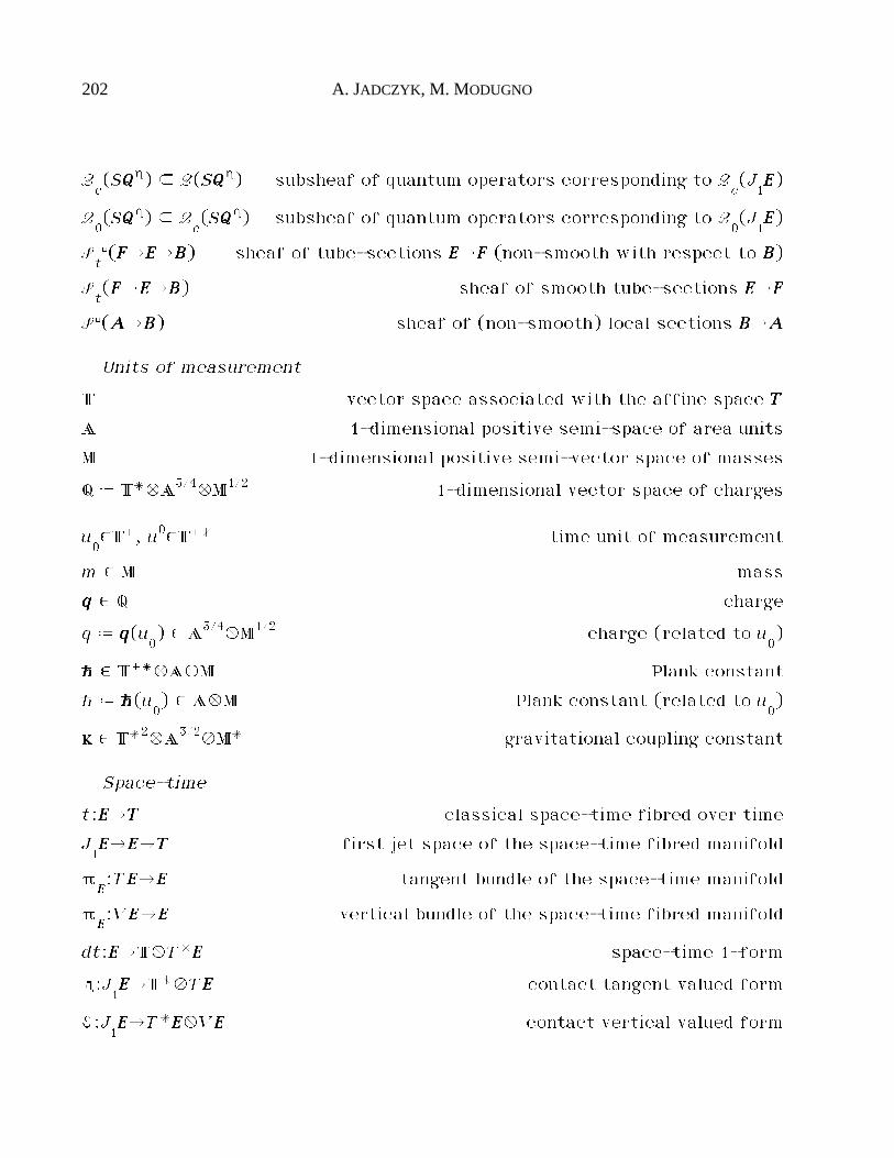
202 A. JADCZYK, M. MODUGNO
Qc(SQQQQ∆) ç Q(SQQQQ∆) subsheaf of quantum operators corresponding to Q
c(J1EEEE)
Q0(SQQQQ∆) ç Q
c(SQQQQ∆) subsheaf of quantum operators corresponding to Q
0(J1EEEE)
St€(FFFFéEEEEéBBBB) sheaf of tube-sections EEEEéFFFF (non-smooth with respect to BBBB)
St(FFFFéEEEEéBBBB) sheaf of smooth tube-sections EEEEéFFFF
S€(AAAAéBBBB) sheaf of (non-smooth) local sections BBBBéAAAA
Units of measurement
T vector space associated with the affine space TTTT
A 1-dimensional positive semi-space of area units
M 1-dimensional positive semi-vector space of masses
Q ˆ T*ÆA3/4ÆM1/2 1-dimensional vector space of charges
u0$T_, u0$T_* time unit of measurement
m $ M mass
qqqq $ Q charge
q ˆ qqqq(u0) $ A3/4ÆM1/2 charge (related to u
0)
hhhh $ T_*ÆAÆM Plank constant
h ˆ hhhh(u0) $ AÆM Plank constant (related to u
0)
kkkk $ T*2ÆA3/2ÆM* gravitational coupling constant
Space-time
t:EEEEéTTTT classical space-time fibred over time
J1EEEEéEEEEéTTTT first jet space of the space-time fibred manifold
πEEEE:TEEEEéEEEE tangent bundle of the space-time manifold
πEEEE:VEEEEéEEEE vertical bundle of the space-time fibred manifold
dt:EEEEéTÆT*EEEE space-time 1-form
d:J1EEEEéT*ÆTEEEE contact tangent valued form
ª:J1EEEEéT*EEEEÆVEEEE contact vertical valued form
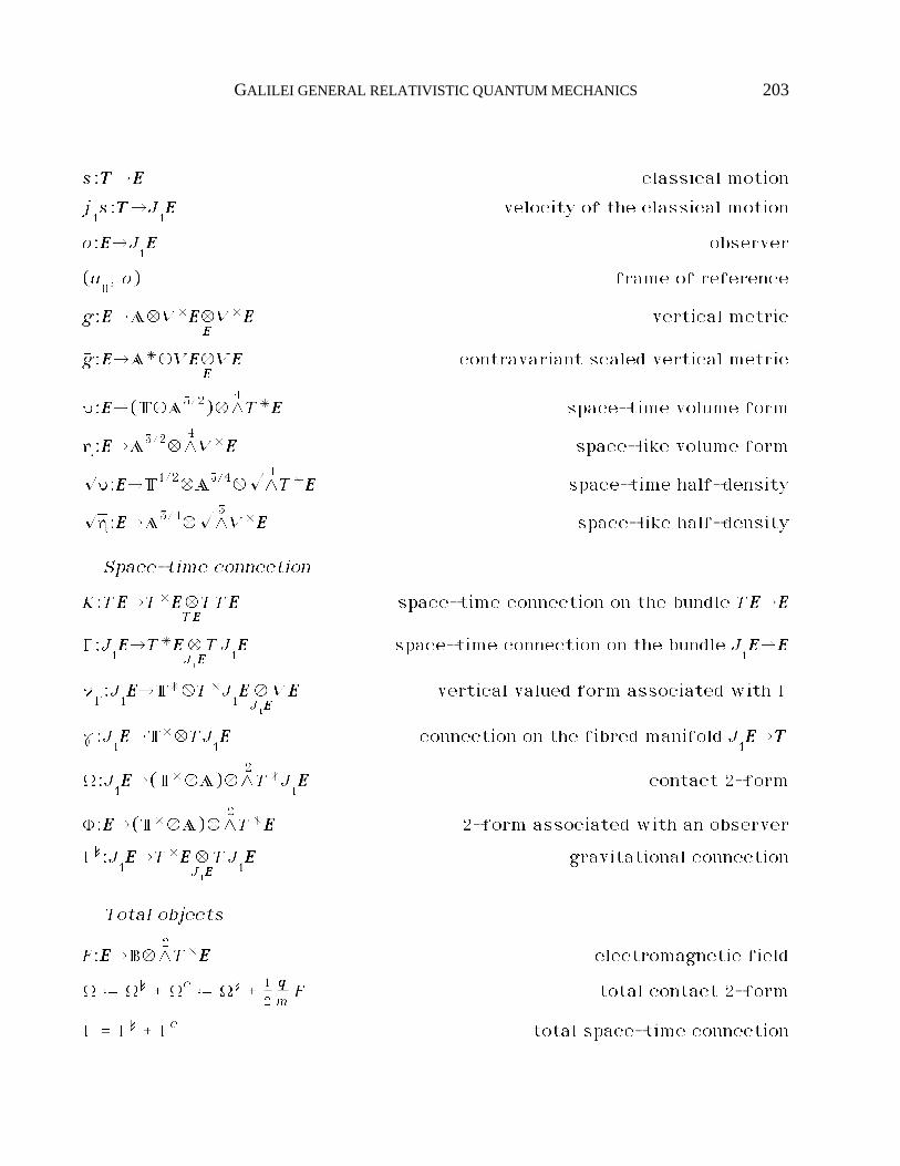
GALILEI GENERAL RELATIVISTIC QUANTUM MECHANICS 203
s:TTTTéEEEE classical motion
j1s:TTTTéJ
1EEEE velocity of the classical motion
o:EEEEéJ1EEEE observer
(u0, o) frame of reference
g:EEEEéAÆV*EEEEÆEEEEV*EEEE vertical metric
ãg:EEEEéA*ÆVEEEEÆEEEEVEEEE contravariant scaled vertical metric
¨:EEEEé(TÆA3/2)ÆL4T*EEEE space-time volume form
∆:EEEEéA3/2ÆL4V*EEEE space-like volume form
¢Ã:EEEEéT1/2ÆA3/4ÆÊL4T*EEEE space-time half-density
¢Ã∆:EEEEéA3/4ÆÊL3V*EEEE space-like half-density
Space-time connection
K:TEEEEéT*EEEEÆTEEEETTEEEE space-time connection on the bundle TEEEEéEEEE
Í:J1EEEEéT*EEEEÆ
J1EEEETJ
1EEEE space-time connection on the bundle J
1EEEEéEEEE
~Í:J1EEEEéT*ÆT*J
1EEEEÆJ1EEEEVEEEE vertical valued form associated with Í
˙:J1EEEEéT*ÆTJ
1EEEE connection on the fibred manifold J
1EEEEéTTTT
Ò:J1EEEEé(T*ÆA)ÆL
2T*J
1EEEE contact 2-form
È:EEEEé(T*ÆA)ÆL2T*EEEE 2-form associated with an observer
ÍŸ:J1EEEEéT*EEEEÆ
J1EEEETJ
1EEEE gravitational connection
Total objects
F:EEEEéBÆL2T*EEEE electromagnetic field
Ò ˆ ÒŸ _ Òe ˆ ÒŸ _ 12qqqqmF total contact 2-form
Í = ÍŸ _ Íe total space-time connection
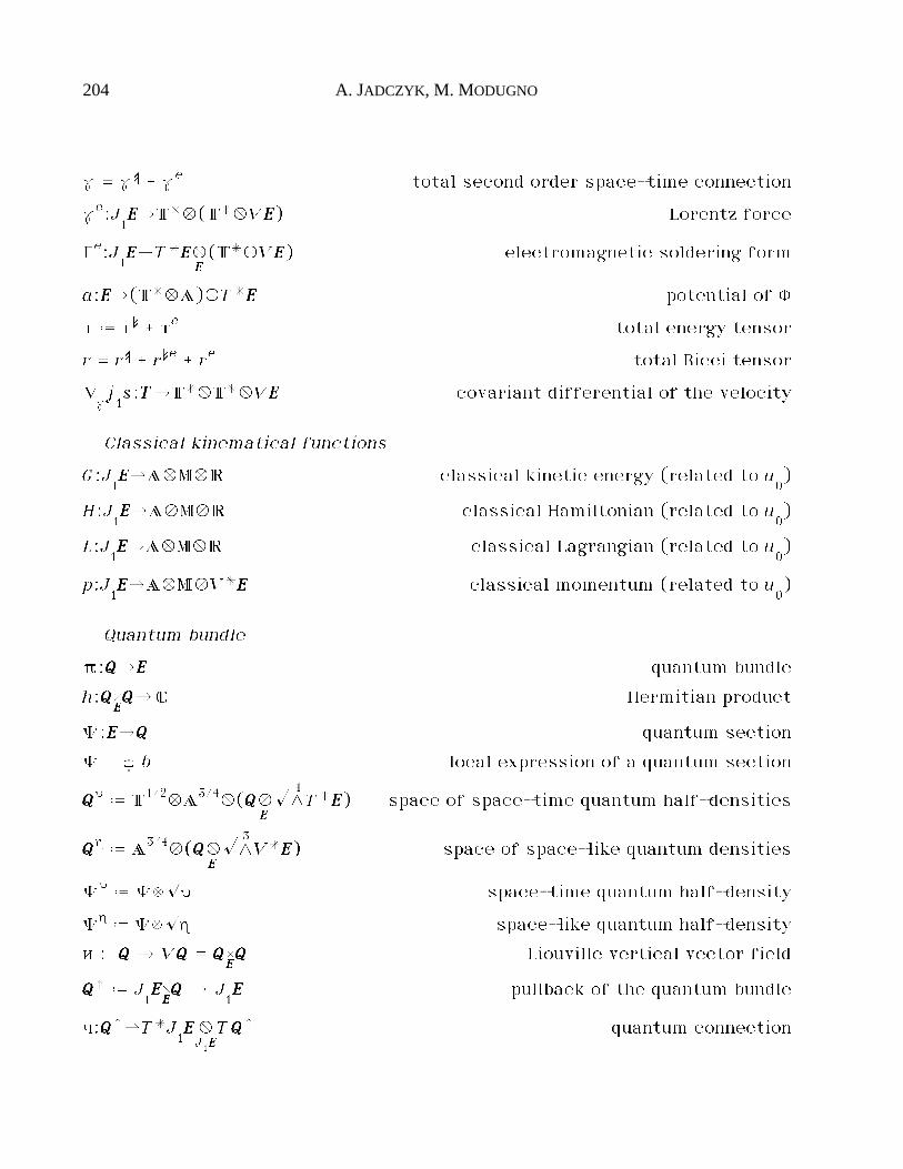
204 A. JADCZYK, M. MODUGNO
˙ = ˙Ÿ _ ˙e total second order space-time connection
˙e:J1EEEEéT*Æ(T*ÆVEEEE) Lorentz force
Íe:J1EEEEéT*EEEEÆ
EEEE(T*ÆVEEEE) electromagnetic soldering form
a:EEEEé(T*ÆA)ÆT*EEEE potential of È
tˆ tŸ _ te total energy tensor
r = rŸ _ rŸe _ re total Ricci tensor
ı j1s:TTTTéT*ÆT*ÆVEEEE covariant differential of the velocity
Classical kinematical functions
G:J1EEEEéAÆMÆ· classical kinetic energy (related to u
0)
H:J1EEEEéAÆMÆ· classical Hamiltonian (related to u
0)
L:J1EEEEéAÆMÆ· classical Lagrangian (related to u
0)
p:J1EEEEéAÆMÆV*EEEE classical momentum (related to u
0)
Quantum bundle
π:QQQQéEEEE quantum bundle
h:QQQQEEEEQQQQéÛ Hermitian product
„:EEEEéQQQQ quantum section
„ = ¥ b local expression of a quantum section
QQQQ¨ ˆ T1/2ÆA3/4Æ(QQQQÆ
EEEEÊL
4T*EEEE) space of space-time quantum half-densities
QQQQ∆ ˆ A3/4Æ(QQQQÆ
EEEEÊL
3V*EEEE) space of space-like quantum densities
„¨ ˆ „æ¢Ã space-time quantum half-density
„∆ ˆ „æ¢Ã∆ space-like quantum half-density
i : QQQQ é VQQQQ = QQQQEEEEQQQQ Liouville vertical vector field
QQQQŸ ˆ J1EEEEEEEEQQQQ é J
1EEEE pullback of the quantum bundle
c:QQQQŸéT*J1EEEEÆJ1EEEETQQQQŸ quantum connection
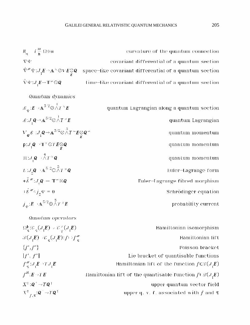
GALILEI GENERAL RELATIVISTIC QUANTUM MECHANICS 205
Rc= i m
hhhhÒæi curvature of the quantum connection
ı„ covariant differential of a quantum section
êı#„:J1EEEEéA*ÆVEEEEÆ
EEEEQQQQ space-like covariant differential of a quantum section
ôı„:J1EEEEéT*ÆQQQQ time-like covariant differential of a quantum section
Quantum dynamics
L„:EEEEéA3/2ÆL
4T*EEEE quantum Lagrangian along a quantum section
L:J1QQQQéA3/2ÆL
4T*EEEE quantum Lagrangian
VQQQQL :J
1QQQQéA3/2ÆL
3T*EEEEÆ
EEEEQQQQ* quantum momentum
p:J1QQQQéT*ÆTEEEEÆ
EEEEQQQQ quantum momentum
∏:J1QQQQéL
4T*QQQQ quantum momentum
E:J2QQQQéA3/2ÆL
5T*QQQQ Euler-Lagrange form
* êE#:J2QQQQ é T*ÆQQQQ Euler-Lagrange fibred morphism
* êE#©j2„ = 0 Schrödinger equation
j„:EEEEéA3/2ÆL
3T*EEEE probability current
Quantum operators
Ò††††@:T
††††(J1EEEE)é T
˙*(J
1EEEE) Hamiltonian isomorphism
F(J1EEEE)éT
††††(J1EEEE):f´f
††††# Hamiltonian lift
f',f" Poisson bracket
[f', f"] Lie bracket of quantisable functions
f#††††:J1EEEEéTJ
1EEEE Hamiltonian lift of the function f$F(J
1EEEE)
fH:EEEEéTEEEE Hamiltonian lift of the quantisable function f$Q(J1EEEE)
XŸ:QQQQŸéTQQQQŸ upper quantum vector field
XŸf,††††:QQQQŸéTQQQQŸ upper q. v. f. associated with f and ††††
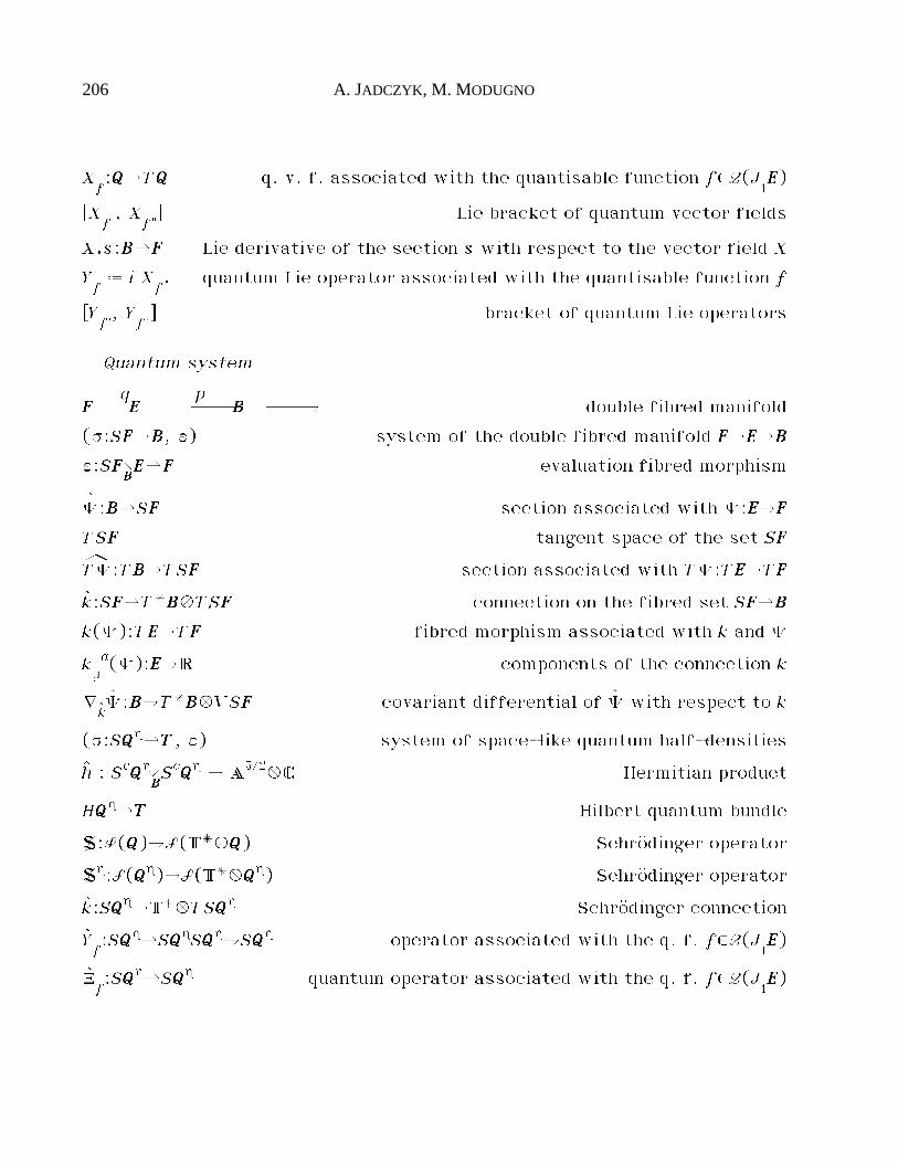
206 A. JADCZYK, M. MODUGNO
Xf:QQQQéTQQQQ q. v. f. associated with the quantisable function f$Q(J
1EEEE)
[Xf', X
f"] Lie bracket of quantum vector fields
X.s:BBBBéFFFF Lie derivative of the section s with respect to the vector field X
Yfˆ i X
f. quantum Lie operator associated with the quantisable function f
[Yf', Y
f"] bracket of quantum Lie operators
Quantum system
FFFF äqEEEE ä
pBBBB double fibred manifold
(ß:SFFFFéBBBB, ™) system of the double fibred manifold FFFFéEEEEéBBBB
™:SFFFFBBBBEEEEéFFFF evaluation fibred morphism
â„:BBBBéSFFFF section associated with „:EEEEéFFFF
TSFFFF tangent space of the set SFFFF
âT„:TBBBBéTSFFFF section associated with T„:TEEEEéTFFFF
âk:SFFFFéT*BBBBÆTSFFFF connection on the fibred set SFFFFéBBBB
k(„):TEEEEéTFFFF fibred morphism associated with k and „
kµa(„):EEEEé· components of the connection k
ıâkâ„:BBBBéT*BBBBÆVSFFFF covariant differential of â„ with respect to k
(ß:SQQQQ∆éTTTT, ™) system of space-like quantum half-densities
hâ : ScQQQQ∆BBBBScQQQQ∆ é A
3/2ÆÛ Hermitian product
HQQQQƎTTTT Hilbert quantum bundle
S:S(QQQQ)éS(T*ÆQQQQ) Schrödinger operator
S∆:S(QQQQ∆)éS(T*ÆQQQQ∆) Schrödinger operator
âk:SQQQQ∆éT*ÆTSQQQQ∆ Schrödinger connection
âYf:SQQQQ∆éSQQQQ∆SQQQQ∆éSQQQQ∆ operator associated with the q. f. f$Q(J
1EEEE)
âÚf:SQQQQ∆éSQQQQ∆ quantum operator associated with the q. f. f$Q(J
1EEEE)
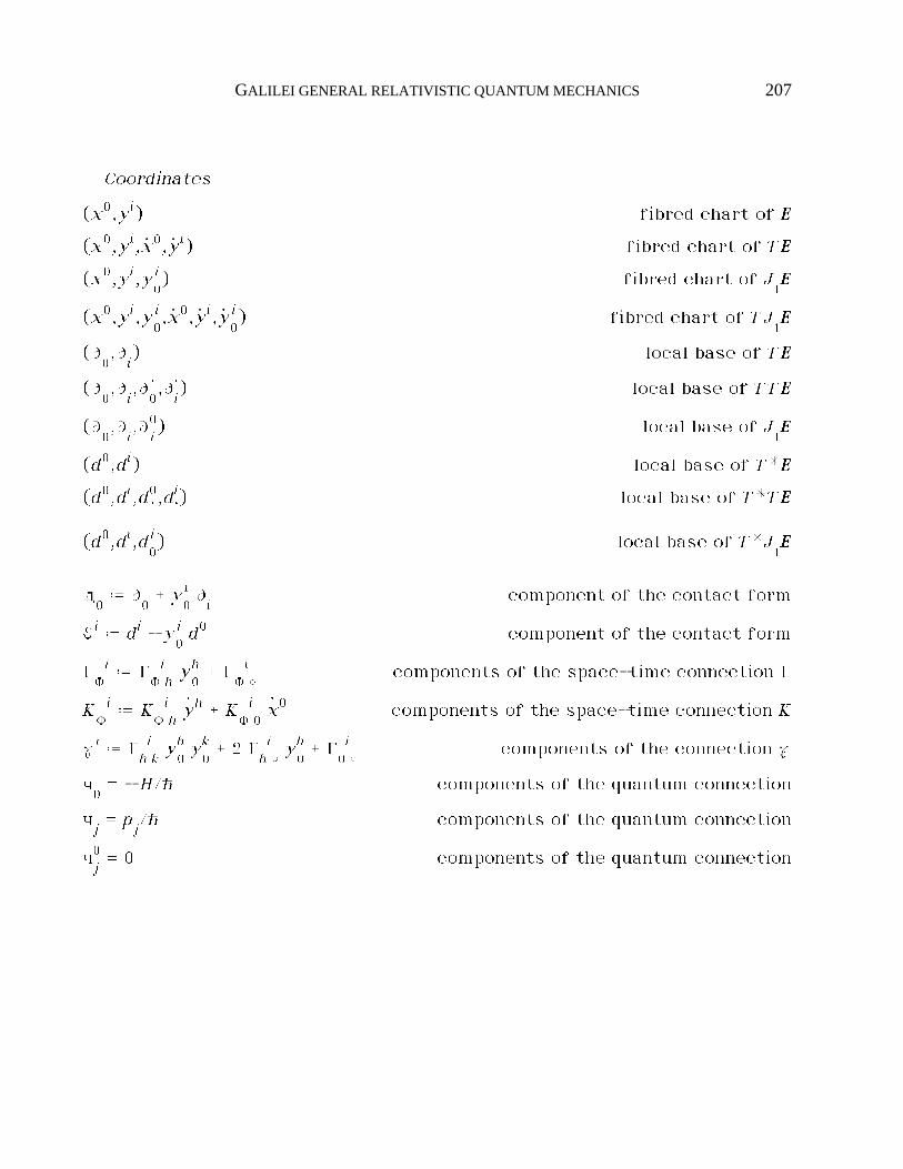
GALILEI GENERAL RELATIVISTIC QUANTUM MECHANICS 207
Coordinates
(x0,yi) fibred chart of EEEE
(x0,yi, îx0, îyi) fibred chart of TEEEE
(x0,yi,y0i) fibred chart of J
1EEEE
(x0,yi,y0i, îx0, îyi, îy
0i) fibred chart of TJ
1EEEE
(Ù0,Ùi) local base of TEEEE
(Ù0,Ùi,Ùî0,Ùîi) local base of TTEEEE
(Ù0,Ùi,Ù
i0) local base of J
1EEEE
(d0,di) local base of T*EEEE
(d0,di,dî0,d
îi) local base of T*TEEEE
(d0,di,d0i) local base of T*J
1EEEE
d0ˆ Ù
0_ y
0i Ù
icomponent of the contact form
ªi ˆ di - y0i d0 component of the contact form
ÍÈi ˆ Í
Èihy0h _ Í
Èi©
components of the space-time connection Í
KÈi ˆ K
Èihîyh _ K
Èi0îx0 components of the space-time connection K
˙i ˆ Íhiky0h y
0k _ 2 Í
hi©y0h _ Í
0i©
components of the connection ˙
c0= - H/h components of the quantum connection
cj= p
j/h components of the quantum connection
c0j= 0 components of the quantum connection
208 A. JADCZYK, M. MODUGNO
IV.2 - Analytic index
(absolute) acceleration: § I.2.6(absolute) motion: § I.1.1(absolute) velocity: § I.1.1absolute time: § I.1.1absolute time function: § I.1.1adapted chart: § I.1.1background connection: § I.6.1charge: § I.3.1charge density: § I.4.5classical constant of motion: § I.5.1classical total objects: § I.3.2classical total energy tensor: § I.4.5classical functions quantistically gauged: § II.1.4classical Lagrangian function: § I.5.2classical Hamiltonian function: § I.5.2classical momentum form: § I.5.2codifferential: § I.2.4connection on a system: § II.5.3connection of order k on a system: § II.5.3contact 2-form: § I.2.5contact structure of jets: § I.1.1Einstein equation: § I.4.7electric field: § I.3.1electromagnetic field: § I.3.1electromagnetic soldering form: § I.3.2Feynmann amplitude: § II.6.5fibred set: § II.5.1first field equation: § I.4.1frame of reference: § I.1.1generalised Newton law of motion: § I.5.1generalised Schrödinger equation: § II.2.3gravitational connection: § I.3.1gravitational coupling constant: § I.1.3Hamiltonian lift: § II.3.1Hermitian connection: § II.1.3
GALILEI GENERAL RELATIVISTIC QUANTUM MECHANICS 209
Hermitian vector field: § II.3.2Hilbert quantum bundle: § II.6.1inertial observer: § I.2.2kinetic energy function: § I.5.2Lie operator: § II.4.1linear connection on a system: § II.5.3Liouville vector fields: § II.1.1Lorentz force: § I.3.2mass: § I.3.1mass density: § I.4.5metrical space-time connection: § I.2.3momentum density: § I.4.5multi-objects: § I.7.1Newton law of gravitation: § I.6.2Newtonian chart: § I.6.2Newtonian connection: § I.6.2Newtonian observer: § I.6.2observed velocity: § I.1.1observer: § I.1.1Planck constant: § II.1.4Poisson Lie bracket: § II.3.1positive semi-vector bundle: § III.1.3positive semi-vector space: § III.1.3pre-Hilbert quantum bundle: § II.6.1pre-quantum system: § II.6.1projectability criterion: § II.1.6quantisable functions: § II.3.1quantum bundle: § II.1.1quantum connection: § II.1.4quantum covariant differential: § II.1.5quantum gauge: § II.1.1quantum Lagrangian: § II.2.1quantum Laplacian: § II.1.5quantum Lie operator: § II.4.2quantum momentum: § II.2.2quantum observed covariant differential: § II.1.5quantum observed Laplacian: § II.1.5quantum observed space-like differential: § II.1.5
210 A. JADCZYK, M. MODUGNO
quantum observed time-like differential: § II.1.5quantum operator: § II.6.3quantum probability current: § II.2.4quantum vector field: § II.3.2Schrödinger operator: § II.2.3second field equation: § I.4.5second order connection: § I.2.5semi-vector bundle: § III.1.3semi-vector space: § III.1.3smooth space in the sense of Frölicher: § II.5.1space of charges: § I.3.1space of masses: § I.3.1space-like volume form: § I.1.2space-like quantum covariant differentials: § II.1.5space-like half-densities quantum bundle: § II.1.2space-time: § I.1.1space-time volume form: § I.1.2space-time connection: § I.2.1space-time half-densities quantum bundle: § II.1.2special space-time: § I.6.3special relativistic Galilei case: § I.6.3system: § II.5.1system of connections: § II.1.3tangent prolongation of a section: § II.5.2tangent space of a system: § II.5.2time component of a quantisable function: § II.3.1time unit of measurement: § I.1.1time-like quantum covariant differential: § II.1.5universal connection: § II.1.3universal curvature: § II.1.3upper quantum vector field: § II.3.2vertical Riemannian metric: § I.1.2
GALILEI GENERAL RELATIVISTIC QUANTUM MECHANICS 211
IV.3 - References
[AM] R. ABRAHAM, J. E. MARSDEN: Foundations of mechanics, 2nd edit.,Benjamin, 1978.
[BMSS] A. P. BALACHANDRAN, G. MARMO, A. SIMONI, G. SPARANO: Quantumbundles and their symmetries, Int. J. Mod. Phys. A, 7777, 8 (1992),1641-1667.
[BFFLS] F. BAYEN, M. FLATO, C. FRONSDAL, A. LICHNEROWICZ, D. STERNHEIMER:Deformation theory and quantization, I and II, Ann. of Phys. III(1978), 61-151.
[Bo] J. BOMAN: Differentiability of a function and of its composition withfunctions of one variable, Math. Scand. 22220000 (1967), 249-268.
[CCKM] A. CABRAS, D. CANARUTTO, I. KOLAR, M. MODUGNO: Structured bundles,Pitagora, Bologna, 1990, 1-100.
[CK] A. CABRAS, I. KOLAR: Connections on some functional bundles, to ap-pear 1993.
[Ca] E. CARTAN: On manifolds with an affine connection and the theory ofgeneral relativity, Bibliopolis, Napoli, 1986.
[Co] P. COSTANTINI: On the geometrical structure of Euler-Lagrange equa-tions, 1993, to appear on Ann. Mat. Pur. Appl..
[Cr] M. CRAMPIN: On the differential geometry of the Euler-Lagrangeequations, and the inverse problem of Lagrangian dynamics, J. Phys.A: Math. Gen 11114444 (1981), 2567-2575.
[CPT] M. CRAMPIN, G. E. PRINCE, G. THOMPSON: A geometrical version of theHelmholtz conditions in time-dependent Lagrangian dynamics, J.Phys. A: Math. Gen 11117777 (1984), 1437-1447.
[dR] G. DE RHAM: Variétés différentiables, Hermann, Paris, 1973.
[DH] H. D. DOMBROWSKI, K. HORNEFFER: Die Differentialgeometrie desGalileischen Relativitätsprinzips, Math. Z. 88886666 (1964), 291.
[Dv1] C. DUVAL: The Dirac & Levy-Leblond equations and geometric quanti-zation, in Diff. geom. meth. in Math. Phys., P.L. García, A. Pérez-Rendón Editors, L.N.M. 1111222255551111 (1985), Springer-Verlag, 205-221.
212 A. JADCZYK, M. MODUGNO
[Dv2] C. DUVAL: On Galilean isometries, Clas. Quant. Grav. 11110000 (1993),2217-2221.
[DBKP] C. DUVAL, G. BURDET, H. P. KüNZLE, M. PERRIN: Bargmann structuresand Newton-Cartan theory, Phys. Rev. D, 33331111, N.8 (1985), 1841-1853.
[DGH] C. DUVAL, G. GIBBONS, P. HORVATY: Celestial mechanics, conformalstructures, and gravitational waves, Phys. Rev. D 44443333, 12 (1991),3907-3921.
[DK] C. DUVAL,, H. P. KüNZLE: Minimal gravitational coupling in theNewtonian theory and the covariant Schrödinger equation, G.R.G.,11116666, 4 (1984), 333-347.
[Eh] J. EHLERS: The Newtonian limit of general relativity, in FisicaMatematica Classica e Relatività, Elba 9-13 giugno 1989, 95-106.
[Fr] A. FRöLICHER: Smooth structures, LNM 999966662222, Springer-Verlag, 1982,69-81.
[GHL] S. GALLOT, D. HULIN, J. LAFONTAINE: Riemannian geometry, secondedition, 1990, Springer Verlag, Berlin.
[Ga] P. L. GARCIA: The Poincaré-Cartan invariant in the calculus of varia-tions, Symposia Mathematica 11114444 (1974), 219-246.
[GS] H. GOLDSMITH, S. STERNBERG: The Hamilton Cartan formalism in thecalculus of variations, Ann. Inst. Fourier, Grenoble, 22223333, 1 (1973),203-267.
[Ha] P. HAVAS: Four-dimensional formulation of Newtonian mechanics andtheir relation to the special and general theory of relativity, Rev.Modern Phys. 33336666 (1964), 938-965.
[Ja] J. JANYSKA: Remarks on symplectic forms in general relativity, 1993,pre-print.
[JM1] A. JADCZYK, M. MODUGNO: An outline of a new geometrical approachto Galilei general relativistic quantum mechanics, in Proceedings ofthe XXI International Conference on Differential Geometric Methodsin Theoretical Physics, Tianjin 5-9 June 1992, Edit. by C. N. Yang, M.L. Ge, X. W. Zhou, World Scientific, 543-556.
[JM2] A. JADCZYK, M. MODUGNO: A scheme for Galilei general relativisticquantum mechanics, 1993, in General Relativity and Gravitational
GALILEI GENERAL RELATIVISTIC QUANTUM MECHANICS 213
Physics, ed. M. Cerdonio, R. D'Auria, M. Francaviglia, G. Magnano,Proc. XXI Conv. Naz. Rel. Gen. Fis. Grav., Bardonecchia (1992), WorldScientific, 1994, 319-337.
[Ke1] X. K EPES : PrinΩip sootvetstviå v ob©ej teorii
otnositelhnosti, Ïurnal ™ksperimentalhnoj i teoreticeskoj
fiziki, (5) 44446666 (1961), 1741-1754.
[Ke2] X. KEPES: Ob©ee reßenie sovmestnoj sistemy uravnenij
‡jnßtejna i uravnenij Nh¨tona, Ïurnal ™ksperimentalhnoj i
teoreticeskoj fiziki, (2) 55550000 (1966), 493-506.
[KS] C. KIEFER, T. P. SINGH: Quantum gravitational corrections to thefunctional Schrödinger equation, Phys. Rev. D 44444444 (1991).
[KS] C. KIEFER: Functional Schrödinger equation for scalar QED, Phys. Rev.D 44445555 (1992), 2044.
[Ko] I. KOLA·: Higher order absolute differentiation with respect to gen-eralised connections, Diff. Geom. Banach Center Publications, 11112222,PWN-Polish Scientific Publishers, Warsaw 1984, 153-161.
[Ku] K. KUCHA·: Gravitation, geometry and nonrelativistic quantum the-ory, Phys. Rev. D, 22222222, 6 (1980), 1285-1299.
[Kü1] H. P. KüNZLE: Galilei and Lorentz invariance of classical particle in-teraction, Symposia Mathematica 11114444 (1974), 53-84.
[Kü2] H. P. KüNZLE: Galilei and Lorentz structures on space-time: compari-son of the corresponding geometry and physics, Ann. Inst. H. Poinc.11117777, 4 (1972), 337-362.
[Kü3] H. P. KüNZLE: Covariant Newtonian limit of Lorentz space-times,G.R.G. 7777, 5 (1976), 445-457.
[Kü4] H. P. KüNZLE: General covariance and minimal gravitational couplingin Newtonian space-time, in Geometrodynamics Proceedings (1983),edit. A. Prastaro, Tecnoprint, Bologna 1984, 37-48.
[KD] H. P. KüNZLE, C. DUVAL: Dirac field on Newtonian space-time, Ann.Inst. H. Poinc., 44441111, 4 (1984), 363-384.
[La] N. P. LANDSMAN: Deformations of algebras of observables and theclassical limit of quantum mechanics, pre-print 1992.
[La] N. P. LANDSMAN, N. LINDEN: The geometry of inequivalent quantiza-
214 A. JADCZYK, M. MODUGNO
tions, Nucl. Phys. B 333366665555 (1991), 121-160.
[LBL] M. LE BELLAC, J. M. LEVY-LEBLOND: Galilean electromagnetism, NuovoCim. 11114444 B, 2 (1973), 217-233.
[Le] J. M. LEVY-LEBLOND: Galilei group and Galilean invariance, in Grouptheory and its applications, E. M. LOEBL Ed., Vol. 2, Academic, NewYork, 1971, 221-299.
[LM] P. LIBERMANN, C.M. MARLE: Symplectic geometry and analytical me-chanics, Reidel, Dordrecht, 1987.
[Li1] A. LICHNEROWICZ: Les variétés de Poisson et leurs algèbres de Lie as-sociées, J. Dif. Geom. 11112222 (1977), 253-300.
[Li1] A. LICHNEROWICZ: Les variétés de Jacobi et leurs algèbres de Lie as-sociées, J. Math. pures et appl. 55557777 (1978), 453-488.
[Ma] L. MANGIAROTTI: Mechanics on a Galilean manifold, Riv. Mat. Univ.Parma (4) 5555 (1979), 1-14.
[MM1] L. MANGIAROTTI, M. MODUGNO: Fibered spaces, jet spaces and connec-tions for field theory, in Proceed. of Int. Meet. on Geometry andPhysics, Pitagora Editrice, Bologna, 1983, 135-165.
[MM2] L. MANGIAROTTI, M. MODUGNO: Connections and differential calculus onfibred manifolds, Pre-print, Dipartimento di Matematica Applicata“G. Sansone”, 1989, 1-142.
[MP1] E. MASSA, E. PAGANI: Classical dynamics of non-holonomic systems:a geometric approach, Ann. Inst. H. Poinc. 55555555, 1 (1991), 511-544.
[MP2] E. MASSA, E. PAGANI: Jet bundle geometry, dynamical connections andthe inverse problem of Lagrangian mechanics, pre-print, 1993, to ap-pear on Ann. Inst. H. Poinc..
[Me] A. MESSIAH: Quantum mechanics, Vol. I, II, III, North-Holland, 1961.
[Mo1] M. MODUGNO: On the structure of classical dynamics, Riv. Univ. Parma(4) 7777 (1981), 409-429.
[Mo2] M. MODUGNO: Systems of vector valued forms on a fibred manifoldand applications to gauge theories, Lect. Notes in Math. 1111222255551111,Springer-Verlag, 1987.
[Mo3] M. MODUGNO: Torsion and Ricci tensor for non-linear connections,Diff. Geom. and Appl. (2) 1111 (1991), 177-192.
GALILEI GENERAL RELATIVISTIC QUANTUM MECHANICS 215
[Pl] W. PAULI: in “Handbuch der Physik” (S. Flügge, ed.), Vol. V, 18-19,Springer, Berlin, 1958.
[Pr1] E. PRUGOVECKI: Quantum geometry. A framework for quantum generalrelativity, Kluwer Academic Publishers, 1992.
[Pr2] E. PRUGOVECKI: On the general covariance and strong equivalenceprinciples in quantum general relativity, pre-print, 1993.
[Sk] J. J. SAKURAI: Modern quantum mechanics, Benjamin 1985.
[Sn] D. J. SAUNDERS: The geometry of jet bundles, Cambridge UniversityPress, 1989.
[Sc] L. L. SCHIFF: Quantum mechanics, McGraw-Hill, Third edition, 1968.
[SP] E. SCHMUTZER, J. PLEBANSKI: Quantum mechanics in non inertialframes of reference, Fortschritte der Physik 22225555 (1977), 37-82.
[Sl] J. SLOVAK: Smooth structures on fibre jet spaces, Czech. Math.Jour., 33336666, 111 (1986), 358-375.
[St] J. SNIATICKI: Geometric quantization and quantum mechanics,Springer, New York, 1980.
[Tr1] A. TRAUTMAN: Sur la théorie Newtonienne de la gravitation, C.R.Acad. Sc. Paris, t. 257 (1963), 617-620.
[Tr2] A. TRAUTMAN: Comparison of Newtonian and relativistic theories ofspace-time, In Perspectives in geometry and relativity (Essays inHonour of V. Hlavaty, N. 42, Indiana Univ. press, 1966, 413-425.
[Tr] M. TRüMPER: Lagrangian mechanics and the geometry of configurationspacetime, Ann. of Phys., 111144449999, (1983), 203-243.
[Tu] W. M. TULCZYJEW: An intrinsic formulation of nonrelativistic analyti-cal mechanics and wave mechanics, J. Geom. Phys., 2222, 3 (1985), 93-105.
[VF] A. M. VERSHIK, L. D. FADDEEV: Lagrangian mechanics in invariantform, Sel. Math. Sov. 4444 (1981), 339-350.
[Wo] N. WOODHOUSE: Geometric quantization, Clarendon Press, Oxford, 2ndEdit. 1992.
Recommended