
Functional Programming I
***Functional Programming andInteractive Theorem Proving
Ulrich Berger
Michaelmas Term 2007

2
***
Room 306 (Faraday Tower)
Phone 513380
Fax 295708
http://www.cs.swan.ac.uk/∼csulrich/
***
MMISS:

3
The aims of this course
• To understand the main concepts of functional programming;
• To solve computational problems using a functional programming
language (we will use Haskell);
• To prove the correctness of functional programs.
MMISS:

4
Recommended Books
• Graham Hutton. Functional Programming in Haskell, Cambridge
University Press, 2006.
• Kees Doets and Jan van Eijck. The Haskell Road to Logic, Maths an
Programming, King’s College Publications, 2004.
• Paul Hudak. The Haskell School of Expression – Learning Functional
Programming through Multimedia. Cambridge University Press, 2000.
MMISS:

5
• Simon Thompson. Haskell: The Craft of Functional Programming, 2nd
edition. Addison-Wesley, 1999.
• Richard Bird. Introduction to Functional Programming using Haskell,
2nd edition. Prentice Hall, 1998.
• Antony J. T. Davie. An Introduction to Functional Programming
Systems Using Haskell, CUP, 1992.
• Jeremy Gibbons and Oege de Moor. The Fun of Programming,
Palgrave Macmillan, 2003 (advanced).
MMISS:

6
Information on the web
• The course web page (contains more links to useful web pages)
http://www.cs.swan.ac.uk/~csulrich/fp1.html
• The Haskell home page
http://www.haskell.org
• Wikipedia
http://en.wikipedia.org
MMISS:

7
Coursework
• Lab classes: Linux lab (room 2007), Monday 12-1, Tuesday 1-2.
Start: 8/10. Computer accounts will be sent by email.
• Coursework counts 20% for CS-221 and 30% for CS-M36 (part 1).
• CS-221: Courseworks 1,2.
• CSM36 (Part 1): Courseworks 1,2,3.
• Submission via coursework box on the 2nd floor.
• Deadlines:
CW1: 17/10 - 1/11, CW2: 14/11 - 29/11, CW3: 21/11 - 6/12.
MMISS:

8
No lecture on Thursday, 11th of October!
MMISS:

9
Overview (Part I)
1. Functional programming: Ideas, results, history, future
2. Types and functions
3. Case analysis, local definitions, recursion
4. Higher order functions and polymorphism
5. The λ-Calculus
6. Lists
7. User defined data types
8. Proofs
MMISS:

1 Functional Programming:Ideas, Results, History, Future

1.1 Ideas 11
1.1 Ideas
• Programs as functions f : Input → Output
No variables — no states — no side effects
All dependencies explicit
Output depends on inputs only, not on environment
Referential Transparancy
MMISS: Ideas

1.1 Ideas 12
• Abstraction
Data abstraction
Function abstraction
Modularisation and Decomposition
• Specification and verification
Typing
Clear denotational and operational semantics
MMISS: Ideas

1.1 Ideas 13
Comparison with other programming paradigms
Imperative Programming state command
Logic Programming specification search
Functional Programming expression evaluation
MMISS:

1.2 Results 14
1.2 Results
The main current functional languages
Language Types Evalution I/O
Lisp, Scheme type free eager via side effects
ML, CAML polymorphic eager via side effects
Haskell, Gofer polymorphic lazy via monads
MMISS:

1.2 Results 15
Haskell, the language we use in this course, is a purely functional
language. Lisp and ML are not purely functional because they allow for
programs with side effects.
Haskell is named after the American Mathematician
Haskell B Curry (1900 – 1982).
Picture on next page copied from
http://www-groups.dcs.st-and.ac.uk/~history
MMISS:

1.2 Results 16
MMISS:

1.2 Results 17
Some areas where functional languages are applied
• Artificial Intelligence
• Scientific computation
• Theorem proving
• Program verification
• Safety critical systems
• Web programming
• Network toolkits and applications
MMISS:

1.2 Results 18
• XML parser
• Natural Language processing and speech recognition
• Data bases
• Telecommunication
• Graphic programming
• Games
http://homepages.inf.ed.ac.uk/wadler/realworld/
MMISS:

1.2 Results 19
Productivity and security
• Functional programming is very often more productive and reliable
than imperative programming
• Ericsson measured an improvement factor of between 9 and 25 in
experiments on telephony software.
• Because of their modularity, transparency and high level of abstraction,
functional programs are particularly easy to maintain and adapt.
• See http://www.haskell.org/aboutHaskell.html
MMISS:

1.2 Results 20
Example: Quicksort
To sort a list with head x and tail xs, compute
• low = the list of all elements in xs that are smaller than x,
• high = the list of all elements in xs that are greater or equal than x.
Then, recursively sort low and high and append the results putting x in
the middle.
MMISS:

1.2 Results 21
Quicksort in Haskell
qsort [] = []qsort (x:xs) = qsort low ++ [x] ++ qsort high
wherelow = [y | y <- xs, y < x]high = [y | y <- xs, y >= x]
MMISS:

1.2 Results 22
Quicksort in C
void qsort(int a[], int lo, int hi)
int h, l, p, t;
if (lo < hi) l = lo;h = hi;p = a[hi];
do while ((l < h) && (a[l] <= p))
MMISS:

1.2 Results 23
l = l+1;while ((h > l) && (a[h] >= p))
h = h-1;if (l < h)
t = a[l];a[l] = a[h];a[h] = t;
while (l < h);
t = a[l];a[l] = a[hi];a[hi] = t;
MMISS:

1.2 Results 24
qsort( a, lo, l-1 );qsort( a, l+1, hi );
MMISS:

1.3 History 25
1.3 History
• Foundations 1920/30
Combinatory Logic and λ-calculus (Schonfinkel, Curry, Church)
• First functional languages 1960
LISP (McCarthy), ISWIM (Landin)
• Further functional languages 1970– 80
FP (Backus); ML (Milner, Gordon), later SML and CAML; Hope
(Burstall); Miranda (Turner)
• 1990: Haskell
MMISS:

1.4 Future 26
1.4 Future
• Functional programming more and more wide spread
• Functional and object oriented programming combined (Pizza, Generic
Java)
• Extensions by dependent types (Chayenne)
• Big companies begin to adopt functional programming
• Microsoft initiative: F# = CAML into .net
MMISS:

2 Types and functions

2 Types and functions 28
Contents
• How to define a function
• How to run a function
• Some basic types and functions
• Pairs and pattern matching
• Infix operators
• Computation by reduction
• Type synonyms
MMISS: Defining functions

2.1 How to define a function 29
2.1 How to define a function
• Example
inc :: Int -> Intinc x = x + 1
• Explanation
1. line: Signature declaring inc as a function expecting an integer as
input and computing an integer as output.
2. line: Definition saying that the function inc computes for any
integer x the integer x + 1.
The symbol x is called a formal parameter,
MMISS: Defining functions

2.1 How to define a function 30
Naming conventions (required)
• Example
inc :: Int -> Intinc x = x + 1
• Functions and formal parameters begin with a lower case letter.
• Types begin with an upper case letter.
MMISS: Defining functions

2.1 How to define a function 31
Definition vs. assignment
The definition
inc x = x + 1
must not be confused with the assignment
x := x + 1
in imperative languages.
MMISS: Defining functions

2.1 How to define a function 32
Functions with more than one argument
Example of a function expecting two arguments.
dSum :: Int -> Int -> IntdSum x y = 2 * (x + y)
A combination of inc and dSum
f :: Int -> Int -> Intf x y = inc (dSum x y)
MMISS: Defining functions

2.1 How to define a function 33
Why types?
• Early detection of errors at compile time
• Compiler can use type information to improve efficiency
• Type signatures facilitate program development
• and make programs more readable
• Types increase productivity and security
MMISS: Running functions

2.2 How to run a function 34
2.2 How to run a function
• hugs is a Haskell interpreter
Small, fast compilation (execution moderate)
Good environment for program development
• How it works
hugs reads definitions (programms, types, . . . ) from a file (script)
Command line mode: Evaluation of expressions
No definitions in command line
• ghci (Glasgow Haskell Compiler Interactive) works similarly.
MMISS: Running functions

2.2 How to run a function 35
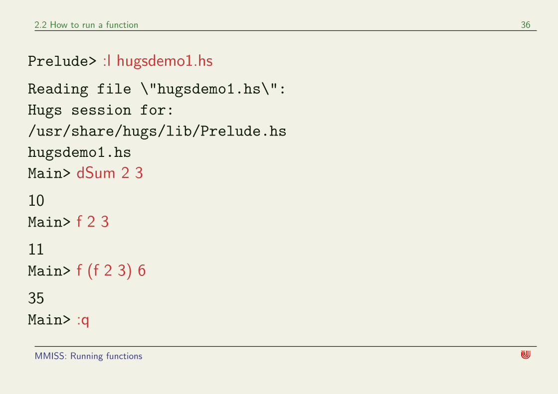
A hugs session
We assume that our example programs are written in a file
hugsdemo1.hs (extension .hs required). After typing
hugs
in a command window in the same directory where our file is, we can run
the following session (black = hugs, red = we)
MMISS: Running functions
2.2 How to run a function 36
Prelude> :l hugsdemo1.hs
Reading file \"hugsdemo1.hs\":Hugs session for:/usr/share/hugs/lib/Prelude.hshugsdemo1.hsMain> dSum 2 3
10
Main> f 2 3
11
Main> f (f 2 3) 6
35
Main> :q
MMISS: Running functions

2.2 How to run a function 37
• At the beginning of the session hugs loads a file Prelude.hs which
contains a bunch of definitions of Haskell types and functions. A copy
of that file is available at our fp1 page. It can be quite useful as a
reference.
• By typing :? (in hugs) one obtains a list of all available commands.
Useful commands are:
:load <filename>
:reload :type <Haskell expression>
:quitAll commands may be abbreviated by their first letter.
MMISS: Running functions

2.2 How to run a function 38
-- That’s how we write short comments
-Longer commentscan be included like this-
MMISS: Running functions

2.2 How to run a function 39
Exercises
• Define a function square that computes the square of an integer
(don’t forget the signature).
• Use square to define a function p16 which raises an integer to its
16th power.
• Use p16 to compute the 16th powers of some numbers between 1 and
10. What do you observe? Try to explain.
MMISS: Basic types and functions

2.3 Some basic types and functions 40
2.3 Some basic types and functions
• Boolean values
• Numeric types: Integers and Floating point numbers
• Characters and Strings
MMISS: Basic types and functions

2.3 Some basic types and functions 41
Boolean values: Bool
• Values True and False
• Predefined functions:
not :: Bool -> Bool negation
(&&) :: Bool -> Bool -> Bool conjunction (infix)
(||) :: Bool -> Bool -> Bool disjunction (infix)
True && False False ( means “evaluates to”)
True || False TrueTrue || True True
MMISS: Basic types and functions

2.3 Some basic types and functions 42
• Example: exclusive disjunction:
exOr :: Bool -> Bool -> BoolexOr x y = (x || y) && (not (x && y))
exOr True True FalseexOr True False TrueexOr False True TrueexOr False False False
MMISS: Basic types and functions

2.3 Some basic types and functions 43
Basic numeric types
Computing with numbers
Limited precision
constant cost←→ arbitrary precision
increasing cost
Haskell offers:
• Int - integers as machine words
• Integer - arbitrarily large integers
• Rational - arbitrarily precise rational numbers
• Float - floating point numbers
• Double - double precision floating point numbers
MMISS: Basic types and functions

2.3 Some basic types and functions 44
Integers: Int and Integer
Some predefined functions (overloaded, also for Integer):
(+), (*), (^), (-) :: Int -> Int -> Int- :: Int -> Int -- unary minusabs :: Int -> Int -- absolute valuediv :: Int -> Int -> Int -- integer divisionmod :: Int -> Int -> Int -- remainder of int. div.
show :: Int -> String
MMISS: Basic types and functions

2.3 Some basic types and functions 45
3 ^ 4 81
4 ^ 3 64
-9 + 4 -5
-(9 + 4) -13
2-(9 + 4) -11
abs -3 error
abs (-3) 3
div 9 4 2
mod 9 4 1
MMISS: Basic types and functions

2.3 Some basic types and functions 46
Comparison operators:
(==),(/=),(<=),(<),(>=),(>) :: Int -> Int -> Bool
-9 == 4 False
9 == 9 True
4 /= 9 True
9 >= 9 True
9 > 9 False
MMISS: Basic types and functions

2.3 Some basic types and functions 47
But also
(==),(/=),(<=),(<),(>=),(>) :: Bool -> Bool -> Bool
True == False False
True == True True
True /= False True
True /= True False
True > False True
False > True False
MMISS: Basic types and functions

2.3 Some basic types and functions 48
Exercise
Recall the definition
exOr :: Bool -> Bool -> BoolexOr x y = (x || y) && (not (x && y))
Give a shorter definition of exOr using a comparison operator.
MMISS: Basic types and functions

2.3 Some basic types and functions 49
Floating point numbers: Float, Double
• Single and double precision Floating point numbers
(IEEE 754 and 854)
• The arithmetic operations (+),(-),(*),- may also be used for
Float and Double
• Float and Double support the same operations
MMISS: Basic types and functions

2.3 Some basic types and functions 50
(/) :: Float -> Float -> Floatpi :: Floatexp,log,sqrt,logBase,sin,cos :: Float -> Float
3.4/2 1.7
pi 3.14159265358979
exp 1 2.71828182845905
log (exp 1) 1.0
logBase 2 1024 10.0
cos pi -1.0
MMISS: Basic types and functions

2.3 Some basic types and functions 51
Conversion from and to integers:
fromIntegral :: Int -> FloatfromIntegral :: Integer -> Floatround :: Float -> Int -- round to nearest integerround :: Float -> Integer
Use signature to resolve overloading:
round 10.7 :: Int
MMISS: Basic types and functions

2.3 Some basic types and functions 52
Example
half :: Int -> Floathalf x = x / 2
Does not work because division (/) expects two floating point numbers
as arguments, but x has type Int.
Solution:
half :: Int -> Floathalf x = (fromIntegral x) / 2
MMISS: Basic types and functions

2.3 Some basic types and functions 53
Characters and strings: Char, String
Notation for characters: ’a’
Notation for characters: ’’hello’’
(:) :: Char -> String -> String -- prefixing(++) :: String -> String -> String -- concatenion
’H’ : "ello W" ++ "orld!" "Hello World!"
: binds stronger than ++
’H’ : "ello W" ++ "orld!" is the same as
(’H’ : "ello W") ++ "orld!"
MMISS: Basic types and functions

2.3 Some basic types and functions 54
Example
rep :: String -> Stringrep s = s ++ s
rep (rep "hello ") "hello hello hello hello "
MMISS: Pairs and pattern matching

2.4 Pairs and pattern matching 55
2.4 Pairs and pattern matching
If a and b are types, then
(a,b)
denotes the cartesian product of a and b(in mathematics usually denoted a× b).
The elements of (a,b) are pairs (x,y) where x is in a and y is in b.
MMISS: Pairs and pattern matching
2.4 Pairs and pattern matching 56
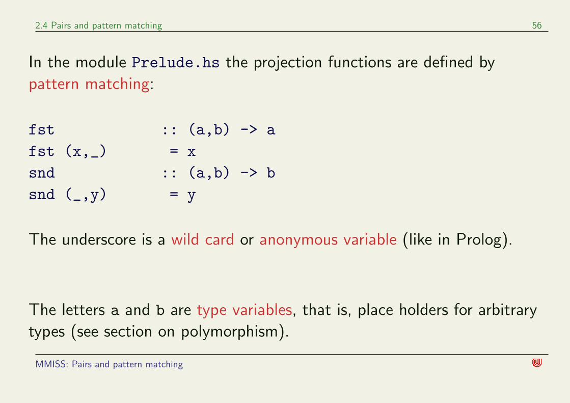
In the module Prelude.hs the projection functions are defined by
pattern matching:
fst :: (a,b) -> afst (x,_) = xsnd :: (a,b) -> bsnd (_,y) = y
The underscore is a wild card or anonymous variable (like in Prolog).
The letters a and b are type variables, that is, place holders for arbitrary
types (see section on polymorphism).
MMISS: Pairs and pattern matching

2.4 Pairs and pattern matching 57
Booleans and numbers can be used for pattern matching as well:
myif :: Bool -> Int -> Int -> Intmyif True n m = nmyif False n m = m
The order of arguments corresponds to the order of types.
myif’ :: Bool -> (Int,Int) -> Intmyif’ True (n,m) = nmyif’ False (n,m) = m
myif expects 3 arguments while myif’ expects only 2 arguments.
MMISS: Pairs and pattern matching

2.4 Pairs and pattern matching 58
Pattern matching with numbers and a wildcard:
myfun :: Int -> Stringmyfun 0 = "Hello"myfun 1 = "world"myfun 2 = "!"myfun _ = ""
The definitions are tried from top to botton.
Therefore, the wildcard _ applies if neither of the numbers 0, 1, 2, match.
MMISS: Infix operators

2.5 Infix operators 59
2.5 Infix operators
• Operators: Names from special symbols !$%&/?+^ . . .
• are written infix: x && y
• otherwise they are normal functions.
MMISS: Infix operators

2.5 Infix operators 60
• Using other functions infix:
x ‘exOr‘ yx ‘dSum‘ y
Note the difference: ‘exOr‘ ’a’
• Operators in prefix notation:
(&&) x y(+) 3 4
MMISS: Computation by reduction

2.6 Computation by reduction 61
2.6 Computation by reduction
• Recall our examples.
inc x = x + 1dSum x y = 2 * (x + y)f x y = inc (dSum x y)
• Expressions are evaluated by reduction.
dSum 6 4 2 * (6 + 4) 20
MMISS: Computation by reduction

2.6 Computation by reduction 62
Evaluation strategy
• From outside to inside, from left to right.
f (inc 3) 4
inc (dSum (inc 3) 4)
(dSum (inc 3) 4) + 1
2*(inc 3 + 4) + 1
2*((3 + 1) + 4) + 1 17
• call-by-need or lazy evaluation
Arguments are calculated only when they are needed.
Lazy evaluation is useful for computing with infinite data structures.
MMISS: Computation by reduction

2.6 Computation by reduction 63
rep (rep "hello ")
rep "hello" ++ rep "hello"
("hello " ++ "hello ") ++ ("hello " ++ "hello ")
"hello hello hello hello"
MMISS: Computation by reduction

2.7 Type synonyms 64
2.7 Type synonyms
Types can be given names to improve readability:
type Ct = Float -- Coordinate
type Pt = (Ct,Ct) -- Point in the plane
swap :: Pt -> Ptswap (x,y) = (y,x)
Note that Haskell identifies the types Pt and (Float,Float).
MMISS: Computation by reduction

2.8 Exercises 65
2.8 Exercises
• Define a function average that computes the average of three
integers.
• Define a function distance that computes the distance of two points
in the plane.
• Define a variant of the distance function where the coordinates are
integers.
• Define exOr using pattern matching.
MMISS: Computation by reduction

2.8 Exercises 66
• Add the missing signatures to the following definitions:
cuberoot x = sqrt (sqrt x)
energy x y = x * y * 9.81
three x y z = x ++ y ++ z
MMISS: Computation by reduction

2.8 Exercises 67
• Consider the following definitions.
f :: Int -> Intf x = f (x+1)
g :: Int -> Int -> Intg x y = y
h :: Int -> Inth x = g (f x) x
What are the results of evaluating f 0 and h 0 ?
MMISS:

3 Case analysis, localdefinitions, recursion

3 Case analysis, local definitions, recursion 69
Content
• Forms of case analysis: if-then-else, guarded equations
• Local definitions: where, let
• Recursion
• Layout
MMISS: Case analysis

3.1 Case analysis 70
3.1 Case analysis
• If-then-else
max :: Int -> Int -> Intmax x y = if x < y then y else x
• Guarded equations
signum :: Int -> Intsignum x
| x < 0 = -1| x == 0 = 0| otherwise = 1
MMISS: Local definitions

3.2 Local definitions 71
3.2 Local definitions
• let
g :: Float -> Float -> Floatg x y = (x^2 + y^2) / (x^2 + y^2 + 1)
better
g :: Float -> Float -> Floatg x y = let a = x^2 + y^2
in a / (a + 1)
MMISS: Local definitions

3.2 Local definitions 72
• where
g :: Float -> Float -> Floatg x y = a / (a + 1) where
a = x^2 + y^2
or
g :: Float -> Float -> Floatg x y = a / b where
a = x^2 + y^2b = a + 1
MMISS: Local definitions

3.2 Local definitions 73
The analoguous definition with let:
g :: Float -> Float -> Floatg x y = let a = x^2 + y^2
b = a + 1in a / b
MMISS: Local definitions

3.2 Local definitions 74
• Local definition of functions
The sum of the areas of two circles with radii r,s.
totalArea :: Float -> Float -> FloattotalArea r s = pi * r^2 + pi * s^2
Use auxiliary function to compute the area of one circle
totalArea :: Float -> Float -> FloattotalArea r s =
let circleArea x = pi * x^2in circleArea r + circleArea s
MMISS: Local definitions

3.2 Local definitions 75
• Locally defined functions may also be written with a type signature:
totalArea :: Float -> Float -> FloattotalArea r s =
let circleArea :: Float -> FloatcircleArea x = pi * x^2
in circleArea r + circleArea s
• Exercise: Use where instead.
MMISS: Recursion

3.3 Recursion 76
3.3 Recursion
• Recursion = defining a function in terms of itself.
fact :: Int -> Intfact n = if n == 0 then 1 else n * fact (n - 1)
Does not terminate if n is negative. Therefore
fact :: Int -> Intfact n
| n < 0 = error "negative argument to fact"| n == 0 = 1| n > 0 = n * fact (n - 1)
MMISS: Recursion

3.3 Recursion 77
• The Fibonacci numbers: 1,1,2,3,5,8,13,21,. . .
fib :: Integer -> Integerfib n
| n < 0 = error "negative argument"| n == 0 || n == 1 = 1| n > 0 = fib (n - 1) + fib (n - 2)
Due to two recursive calls this program has exponential run time.
MMISS: Recursion

3.3 Recursion 78
• A linear Fibonacci program with a subroutine computing pairs of
Fibonacci numbers:
fib :: Integer -> Integerfib n = fst (fibpair n) where
fibpair :: Integer -> (Integer,Integer)fibpair n| n < 0 = error "negative argument to fib"| n == 0 = (1,1)| n > 0 = let (k,l) = fibpair (n - 1)
in (l,k+l)
MMISS: Layout

3.4 Layout 79
3.4 Layout
Due to an elaborate layout Haskell programs do not need many brackets
and are therefore well readable. The layout rules are rather intuitive:
• Definitions must start at the beginning of a line
• The body of a definition must be indented against the function
defined,
• lists of equations and other special constructs must properly line up.
MMISS: Computation by reduction

3.5 Exercises 80
3.5 Exercises
• Define recursively a function euler such that for every nonnegative
integer n and every real number x (given as a floating point number)
euler n x =n∑
k=0
xk
k!
For negative n the result shall be an error.
• Analyse the behaviour of euler n x when n increases and x is fixed (for
example x = 1).
MMISS:

4 Higher order functions andPolymorphism

4 Higher order functions and Polymorphism 82
Contents
• Function types
• Higher order functions
• Polymorphic functions
• Type classes and overloading
• Lambda abstraction
MMISS: Higher order functions and polymorphism Label

4.1 Function types 83
4.1 Function types
Consider the function
add :: Int -> Int -> Intadd x y = x + y
The signature of add is shorthand for
add :: Int -> (Int -> Int)
MMISS: Higher order functions and polymorphism Label

4.1 Function types 84
We may, for example, define
addFive :: Int -> IntaddFive = add 5
add :: Int -> (Int -> Int)addFive = add 5 :: Int -> IntaddFive 7 :: Int
Therefore
addFive 7 (add 5) 7 = add 5 7 5+7 12
MMISS: Higher order functions and polymorphism Label

4.1 Function types 85
• Int -> Int is a function type.
• Function types are ordinary types,
• they may occur as result types
(like in Int -> (Int -> Int)),
• but also as argument types:
twice :: (Int -> Int) -> Int -> Inttwice f x = f (f x)
twice addFive 7 addFive (addFive 7) . . . 17
MMISS: Higher order functions and polymorphism Label

4.1 Function types 86
• type1 -> type2 -> ... -> typen -> type
is shorthand for
type1 -> (type2 -> ... -> (typen -> type)...)
• f x1 x2 ... xn
is shorthand for
(...((f x1) x2) ... ) xn
MMISS: Higher order functions and polymorphism Label

4.1 Function types 87
Sections
If we apply a function of type, say
f :: type1 -> type2 -> type3 -> type4 -> type5
to arguments, say, x1 and x2, then
x1 must have type type1, x2 must have type type2.
and we get
f x1 x2 :: type3 -> type4 -> type5
The expression f x1 x2 is called a section of f.
For example add 5 is a section of add because
add :: Int -> Int -> Intadd 5 :: Int -> Int
MMISS: Higher order functions and polymorphism Label

4.1 Function types 88
• Applying a function n-times:
iter :: Int -> (Int -> Int) -> Int -> Intiter n f x
| n == 0 = x| n > 0 = f (iter (n-1) f x)| otherwise = error "negative argument to iter"
Informally, iter n f x = f ( .... (f x)...) with n applications
of f.
MMISS: Higher order functions and polymorphism Label

4.1 Function types 89
iter 3 addFive 7 addFive (iter 2 addFive 7) (iter 2 addFive 7) + 5 addFive (iter 1 addFive 7) + 5 (iter 1 addFive 7) + 5 + 5 addFive (iter 0 addFive 7) + 5 + 5 (iter 0 addFive 7) + 5 + 5 + 5 7 + 5 + 5 + 5 22
MMISS: Higher order functions and polymorphism Label

4.1 Function types 90
• If a functions has a function type as argument type, then it is called a
higher-order function,
• otherwise it is called a first-order function.
• twice and iter are higher-order functions whereas add and the
functions we discussed in previous chapters were first-order functions.
MMISS: Higher order functions and polymorphism Label

4.2 Polymorphism 91
4.2 Polymorphism
Another important difference between the functions
add :: Int -> Int -> Intadd x y = x + y
and
twice :: (Int -> Int) -> (Int -> Int)twice f x = f (f x)
is that while in the signature of add the type Int was special (we could
not have replaced it by, say, Char), in the signature of twice the type
Int was irrelevant.
MMISS: Higher order functions and polymorphism Label

4.2 Polymorphism 92
• In Haskell we can express the latter fact by assigning twice a
polymorphic type, that is, a type that contains type variables:
twice :: (a -> a) -> (a -> a)twice f x = f (f x)
twice then becomes a polymorphic function.
MMISS: Higher order functions and polymorphism Label

4.2 Polymorphism 93
• Type variable begin with a lower case letter.
• Polymorphic functions can be used in any context where the type
variables can be substituted by suitable types such that the whole
expression is well typed.
MMISS: Higher order functions and polymorphism Label

4.2 Polymorphism 94
Exercise
Check the types of the following expressions and compute their values:
twice square 2twice twice square 2
MMISS: Higher order functions and polymorphism Label

4.2 Polymorphism 95
Type check:
twice :: (a -> a) -> (a -> a)twice :: (Int -> Int) -> (Int -> Int)square :: Int -> Int2 :: Int
therefore
twice square 2 :: Int
MMISS: Higher order functions and polymorphism Label

4.2 Polymorphism 96
Computation:
(twice square) 2 square (square 2) (square 2)2
(22)2 16
MMISS: Higher order functions and polymorphism Label

4.2 Polymorphism 97
Type check:
twice :: ( a -> a )->( a -> a )twice :: ((Int->Int)->(Int->Int))->((Int->Int)->(Int->Int))twice :: (Int->Int)->(Int->Int)square :: Int->Int2 :: Int
therefore
twice twice square 2 :: Int
MMISS: Higher order functions and polymorphism Label

4.2 Polymorphism 98
Computation:
((twice twice) square) 2
(twice (twice square)) 2
(twice square) ((twice square) 2)
square (square ((twice square) 2))
(square ((twice square) 2))2
(((twice square) 2)2)2
. . . (((22)2)2)2
. . . 216 = 65536
MMISS: Higher order functions and polymorphism Label

4.2 Polymorphism 99
Some predefined polymorphic functions
• Identity (more useful than one might think)
id :: a -> aid x = x
• Projections
fst :: (a,b) -> afst (x,_) = x
snd :: (a,b) -> asnd (_,y) = y
MMISS: Higher order functions and polymorphism Label

4.2 Polymorphism 100
• Composition
(.) :: (b -> c) -> (a -> b) -> (a -> c)(f . g) x = f (g x)
• Currying and Uncurrying
curry :: ((a,b) -> c) -> (a -> b -> c)curry f x y = f (x,y)
uncurry :: (a -> b -> c) -> ((a,b) -> c)uncurry f (x,y) = f x y
MMISS: Higher order functions and polymorphism Label

4.2 Polymorphism 101
Exercises
In Haskell’s Prelude.hs the function uncurry is defined slightly
differently:
uncurry :: (a -> b -> c) -> ((a,b) -> c)uncurry f p = f (fst p) (snd p)
instead of
uncurry f (x,y) = f x y
Can you explain why?
MMISS: Higher order functions and polymorphism Label

4.2 Polymorphism 102
Prove that the functions curry and uncurry are inverse to each other,
that is
uncurry (curry f) = fcurry (uncurry g) = g
for all f :: (a,b) -> c and g :: a -> b -> c.
We verify the equations for all possible arguments:
uncurry (curry f) (x,y) = curry f x y = f (x,y)
curry (uncurry g) x y = uncurry g (x,y) = g x y
MMISS: Higher order functions and polymorphism Label

4.2 Polymorphism 103
Extensionality
Two functions are equal when they are equal at all arguments, that is,
f = f’ if and only if f z = f’ z for all z.
MMISS: Higher order functions and polymorphism Label

4.2 Polymorphism 104
• Until: Repeatedly applying an operation f to an initial value x until a
property p x holds (predefined).
until :: (a -> Bool) -> (a -> a) -> a -> auntil p f x =
if p x then x else until p f (f x)
MMISS: Higher order functions and polymorphism Label

4.2 Polymorphism 105
Example: Given f :: Int -> Int, find the least n >= 0 such that
f n <= f (n+1).
nondecreasing :: (Int -> Int) -> Intnondecreasing f = until nondec inc 0 where
nondec n = f n <= f (n+1)inc n = n+1
What is the value of nondecreasing f for
f :: Int -> Intf x = x^2 - 6*x
MMISS: Higher order functions and polymorphism Label

4.2 Polymorphism 106
Exercise
Compute for any function f :: Int -> Int and m >= 0 the maximum
of the values f 0, ..., f m.
maxfun :: (Int -> Int) -> Int -> Intmaxfun f m
|m < 0 = error "negative argument to maxfun"|m == 0 = f 0|m > 0 = max (maxfun f (m-1)) (f m)
Here we used the predefined function max.
MMISS: Higher order functions and polymorphism Label

4.3 Type Classes and Overloading 107
4.3 Type Classes and Overloading
In Hugs one can find out the type of an expression by typing, for example:
Hugs> :t TrueTrue :: Bool
Hugs> :t (&&)(&&) :: Bool -> Bool -> Bool
(:t is shorthand for :type)
MMISS: Higher order functions and polymorphism Label

4.3 Type Classes and Overloading 108
Also polymorphic functions may be queried for their types:
Hugs> :t fstfst :: (a,b) -> a
Hugs> :t currycurry :: ((a,b) -> c) -> a -> b -> c
MMISS: Higher order functions and polymorphism Label

4.3 Type Classes and Overloading 109
Asking for the type of numeric expressions we get the following:
Hugs> :t 00 :: Num a => a
Hugs> :t (+)(+) :: Num a => a -> a -> a
What does Num a => mean?
MMISS: Higher order functions and polymorphism Label

4.3 Type Classes and Overloading 110
Type classes and bounded polymorphism
The fact that the type of (+) is
(+) :: Num a => a -> a -> a
means that (+) is a function of two arguments that can be used with
any type a which is member of the type class Num.
Hence (+) is polymorphic, but its polymorphism is bounded by the type
class Num.
All overloading in Haskell is implemented via type classes.
MMISS: Higher order functions and polymorphism Label

4.3 Type Classes and Overloading 111
More about type classes
We can find out more about the type class Num by typing:
Hugs> :i Num-- type classinfixl 6 +infixl 6 -infixl 7 *class (Eq a, Show a) => Num a where
(+) :: a -> a -> a(-) :: a -> a -> a(*) :: a -> a -> anegate :: a -> a
MMISS: Higher order functions and polymorphism Label

4.3 Type Classes and Overloading 112
abs :: a -> asignum :: a -> afromIntegral :: (Integral a, Num b) => a -> b
-- instances:instance Num Intinstance Num Integerinstance Num Floatinstance Num Doubleinstance Integral a => Num (Ratio a)
MMISS: Higher order functions and polymorphism Label
4.3 Type Classes and Overloading 113
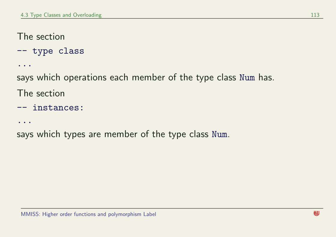
The section
-- type class...
says which operations each member of the type class Num has.
The section
-- instances:...
says which types are member of the type class Num.
MMISS: Higher order functions and polymorphism Label

4.3 Type Classes and Overloading 114
The line
class (Eq a, Show a) => Num a where
says that each Num inherits all operations from the type classes Eq and
Show.
The line
fromIntegral :: (Integral a, Num b) => a -> b
says that for any type a in the type class Integral and any type b in
the type class Num there is a function
fromIntegral :: a -> b
MMISS: Higher order functions and polymorphism Label

4.3 Type Classes and Overloading 115
Later in the course you will learn how to
• put a type into a type class;
• create your own type class.
MMISS: Higher order functions and polymorphism Label

4.3 Type Classes and Overloading 116
Exercise
Find out more about the following type classes:
• Eq
• Show
• Ord
• Integral
MMISS: Higher order functions and polymorphism Label

4.4 λ-Abstraction 117
4.4 λ-Abstraction
Using λ-abstraction we can create anonymous functions, that is,
functions without name.
For example, instead of defining at top level the test function
f :: Int -> Intf x = x^2 - 6*x
(which is not of general interest) and then running
Main> nondecreasing f
we may simply run
Main> nondecreasing (\x -> x^2 - 6*x)
MMISS: Higher order functions and polymorphism Label

4.4 λ-Abstraction 118
In general an expression
\x -> <...>
is equivalent to
let f x = <...>in f
λ-abstraction is not needed, strictly speaking, but often very handy.
MMISS: Higher order functions and polymorphism Label

4.4 λ-Abstraction 119
Examples of λ-abstraction
• λ-abstraction in definitions:
square :: Int -> Intsquare = \x -> x*x
(instead of square x = x*x)
• Pattern matching in λ-abstraction:
swap :: (a,b) -> (b,a)swap = \(x,y) -> (y,x)
(instead of swap (x,y) = (y,x))
MMISS: Higher order functions and polymorphism Label

4.4 λ-Abstraction 120
• Avoiding local definitions by λ-abstraction (not always recommended):
nondecreasing :: (Int -> Int) -> Intnondecreasing f = until (\n -> f n <= f (n+1))
(\n -> n+1)0
instead of
nondecreasing f = until nondec inc 0 wherenondec n = f n <= f (n+1)inc n = n+1
MMISS: Higher order functions and polymorphism Label

4.4 λ-Abstraction 121
• Higher-order λ-abstraction (that is, the abstracted parameter has a
higher-order type):
quad :: Int -> Intquad = twice square
can be defined alternatively by
quad = (\f -> \x -> f (f x)) (\x -> x*x)
MMISS: Higher order functions and polymorphism Label

4.4 λ-Abstraction 122
The type of a λ-abstraction
If we have an expression of type
<...> :: type2
and the parameter x has type type1, then the lambda abstraction has
type
(\x -> <...>) :: type1 -> type2
MMISS:

5 The λ-Calculus

5 The λ-Calculus 124
Contents
• Historical background
• Syntax
• Operational Semantics
• Some fundamental questions
• Normalisation
• Uniqueness of normal forms
• Reduction strategies
• Universality of the λ-calculus
• Typed λ-calculi
MMISS: The λ-calculus

5.1 Historical background 125
5.1 Historical background
The λ-calculus is a formal system capturing the ideas of function
abstraction and application. It was introduced by Alonzo Church and
Haskell B Curry in the 1930s.
It has deep connections with logic and proofs and plays an important role
in the development of Philosophy, Logic, and Computer Science.
MMISS: The λ-calculus

5.1 Historical background 126
In the following, the fundamentals of the λ-calculus will be outlined and
the main results highlighted.
The study of the λ-calculus will give us an appreciation of the historical
and philosophical context of functional programming and will help us in
better understanding the power and elegance of functional concepts.
MMISS: The λ-calculus

5.2 Syntax 127
5.2 Syntax
λ-terms are defined by the grammar
M ::= x | (λx M) | (M N)
Conventions:
• We omit outermost brackets.
• M N K means ((M N) K) e.t.c.
• λx .M N K means λx ((M N) K) e.t.c.
MMISS: The λ-calculus

5.2 Syntax 128
Lambda-calculus vs. Haskell
We may view λ-terms as Haskell expressions, if we read
“λx M” as “\x -> M”.
In fact, Haskell is an applied form of the λ-calculus.
MMISS: The λ-calculus

5.2 Syntax 129
Free variables
The set of free variables of a term M , denoted FV(M), is the set of
variables x in a term that are not in the scope of a λ-abstraction, λx.
Example: FV((λx . y x)(λy . z y)) = y, z
Note that in the example the variable y has a free and a bound
ocurrence.
MMISS: The λ-calculus

5.2 Syntax 130
Substitution
Substitution: M [N/x] is the result of replacing in M every free
occurrence of x by N , renaming, if necessary, bound variables in M in
order to avoid “variable clashes”.
Instead of M [N/x] some authors write M [x/N ], or M [x := N ].
Example:
((λx . y x)(λy . z y))[(x z) / y] = (λx′.(x z) x′)(λy . z y)
The following literal replacement would be wrong:
((λx . y x)(λy . z y))[(x z) / y] = (λx.(x z) x)(λy . z y)
MMISS: The λ-calculus

5.3 Operational Semantics 131
5.3 Operational Semantics
Conversions
• (α) λx .M → λy . (M [y/x]) provided y 6∈ FV(M).
• (β) (λx .M) N →M [N/x].
• (η) λx .M x→M provided x 6∈ FV(M).α-conversion expresses bound renaming
β-conversion expresses computation
η-conversion expresses extensionality
We will concentrate on β-conversion.
We will identify terms that can be transformed into each other by
α-conversions (α-variants).
MMISS: The λ-calculus

5.3 Operational Semantics 132
Reduction
β-reduction means carrying out a β-conversion inside a term, that is
C[(λx M) N ] → C[M [N/x]]
where C[.] denotes a ‘term context’.
In the following ‘reduction’ means ‘β-reduction’ and ‘M → N ′ means
that M β-reduces to N .
MMISS: The λ-calculus

5.3 Operational Semantics 133
Normal forms
A term is in β-normal form (or normal form, for short), if it cannot be
reduced.
Examples: λx . x x is in normal form. (λx . x) x is not in normal form.
A term N is the normal form of another term M if N is in normal form
and there is a reduction chain from M to N , that is,
M →M1→ . . .→Mk → N
for some terms M1, . . . ,Mk.
MMISS: The λ-calculus

5.3 Operational Semantics 134
Example: Set M := λfλx . f (f x) (= program twice).
M M = (λfλx . f (f x))(λfλx . f (f x))→ λx . (λfλx . f (f x))((λfλx . f (f x))x)→ λx . (λfλx . f (f x))(λy . x (x y))→ λx . λz . (λy . x (x y))((λy . x (x y)) z)→ λx . λz . (λy . x (x y)) (x (x z))→ λx . λz . x (x (x (x z))) (this is in normal form)
Hence M M has normal form λx . λz . x (x (x (x z))).
MMISS: The λ-calculus

5.4 Some fundamental questions 135
5.4 Some fundamental questions
• Does every term have a normal form?
• Is the normal form unique?
• Which reduction strategies are good, which are bad?
• Which kinds of computations can be done with the λ-calculus?
MMISS: The λ-calculus

5.5 Normalisation 136
5.5 Normalisation
Not every term has a normal form:
Set ω := λx . x x and Ω := ω ω. Then
Ω = (λx . x x) (λx . x x)→ (λx . x x) (λx . x x)→ . . .
Hence, Ω has no normal form.
MMISS: The λ-calculus

5.5 Normalisation 137
• A term is weakly normalising if it has a normal form.
• A term is strongly normalising if every reduction sequence terminates
(with a normal form).
• Exercise: Find terms that are
not weakly normalising;
weakly, but not strongly normalising;
strongly normalising.
MMISS: The λ-calculus

5.6 Uniqueness of normal forms 138
5.6 Uniqueness of normal forms
• Theorem (Church/Rosser) β-reduction is confluent (or has the
Church-Rosser property). This means: If M →∗ M1 and M →∗ M2,
then there is a term M3 such that M1→∗ M3 and M2→∗ M3
M@
@@@R
∗∗M2M1
@@
@@R ∗∗M3
• Corollary: Every term has at most one normal form.
MMISS: The λ-calculus

5.7 Reduction strategies 139
5.7 Reduction strategies
Rightmost-innermost or eager reduction (Lisp, Scheme, ML)
• Advantages: Avoids repeated computations; computation cost easy to
analyze.
• Disadvantages: May perform unnecessary computations; if divergence
(non-termination) possible, then eager reduction does diverge.
MMISS: The λ-calculus
5.7 Reduction strategies 140
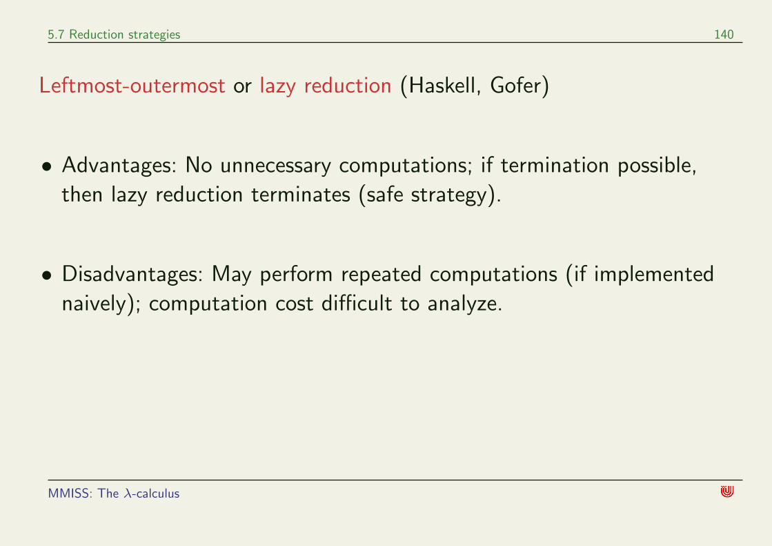
Leftmost-outermost or lazy reduction (Haskell, Gofer)
• Advantages: No unnecessary computations; if termination possible,
then lazy reduction terminates (safe strategy).
• Disadvantages: May perform repeated computations (if implemented
naively); computation cost difficult to analyze.
MMISS: The λ-calculus

5.7 Reduction strategies 141
Example
In a previous reduction chain we used the ‘rightmost-innermost’, or
‘eager’ reduction strategy.
Now let us reduce the same term M M using ‘leftmost-outermost’, or
‘lazy’ reduction which is the strategy Haskell uses.
MMISS: The λ-calculus

5.7 Reduction strategies 142
M M = (λfλx . f (f x))(λfλx . f (f x))→ λx . (λfλx . f (f x))((λfλx . f (f x))x)→ λx . λy . ((λfλx . f (f x))x) (((λfλx . f (f x))x) y)→2 λx . λy . (λz . x (x z))((λz . x (x z)) y)→ λx . λy . x (x ((λz . x (x z)) y))→ λx . λy . x (x (x (x y)))
MMISS: The λ-calculus

5.8 Universality of the λ-calculus 143
5.8 Universality of the λ-calculus
• Theorem (Kleene) The λ-calculus is a universal model of
computation.
• This means:
Data can be encoded by λ-terms, for example n ∈ N is encoded by
the Church Numeral cn := λf.λx.f(f . . . (fx) . . .) (n times ‘f ’).
Given a computable function f : N→ N, there is a λ-term M such
that for all n
M(cn)→∗ cf(n)
MMISS: The λ-calculus

5.8 Universality of the λ-calculus 144
Key idea of the proof: Find a λ-term that performs recursion:
Y := λf . (λx . f (xx)) (λx . f (xx))
Y is a fixed point combinator: For every term M
Y M =β M (Y M)
where N =β K means that N and K can be reduced to a common
term, that is N →∗ L and K →∗ L for some term L.
MMISS: The λ-calculus

5.8 Universality of the λ-calculus 145
Indeed if Y := λf . (λx . f (xx)) (λx . f (xx)) then
Y M → (λx .M(xx)) (λx .M(xx))
→ M ((λx .M(xx)) (λx .M(xx))
But also
M (Y M) → M ((λx .M(xx)) (λx .M(xx))
MMISS: The λ-calculus

5.8 Universality of the λ-calculus 146
Using the fixed point combinator Y it is possible to encode any Turing
machine.
The surprising computational power of the λ-calculus triggered the
development of functional programming languages.
Modern implementations do not use β-reduction, literally, but are based
on related, but more efficient models like, for example, Krivine’s Abstract
Machine, SECD-machines, or Graph Reduction (see, for example, Davie’s
book).
MMISS: The λ-calculus

5.9 Typed λ-calculi 147
5.9 Typed λ-calculi
Typing is a way of assigning meaning to a term.
A typing judgement is of the form
x1 : a1, . . . , xn : an `M : b
It means (intuitively) if x1 has type a1 e.t.c., then M has type b.
The sequence x1 : a1, . . . , xn : an is called a context.
It is common to use the letter Γ as a name for a context.
MMISS: The λ-calculus

5.9 Typed λ-calculi 148
Basic typing rules
The three basic typing rules are:
Γ, x : a ` x : a
Γ, x : a `M : b
Γ ` λx M : a→ b
Γ `M : a→ b Γ ` N : a
Γ `M N : b
These rules define the simply typed λ-calculus.
MMISS: The λ-calculus

5.9 Typed λ-calculi 149
For example
M : a→ b
corresponds to Haskell’s
M :: a -> b
MMISS: The λ-calculus

5.9 Typed λ-calculi 150
Strong normalisation via typing
Theorem (Turing, Girard, Tait, Troelstra. . . ) Every typeable term is
strongly normalizing.
This theorem extends to
• terms containing recursively defined functions which perform recursive
calls at smaller arguments only.
• a variety of type systems, including large fragments of Haskell and ML.
MMISS: The λ-calculus

5.9 Typed λ-calculi 151
Type inference
Haskell and ML use elaborate type inference systems (finding a context
Γ and type a such that Γ `M : a). Type inference was introduced by
Roger Hindley.
Theorem (Hindley) It is decidable whether a term is typeable. If a term
is typeable, its principal type (that is, most general type) can be
computed.
Exercise: What is the most general type of λf.λg.λx.g(fx)?
MMISS: The λ-calculus

5.9 Typed λ-calculi 152
Books on the λ-calculus
• Comprehensive and very readable expositions of the Lambda-calculus
can be found in the books
H Barendregt, The Lambda Calculus - Its Syntax and Semantics,
North Holland, 1984
R Hindley and J P Seldin, Introduction to Combinators and
λ-calculus London Mathematical Society, Student Texts 1,
Cambridge University Press, 1986
• The cited textbooks on Functional Programming by Bird, Davie and
Thompson contain chapters about the λ-calculus and further pointers
to the literature.
MMISS:

6 Lists

6 Lists 154
Contents
• Lists in Haskell
• Recursion on lists
• Higher-order functions on lists
• List comprehension
• Examples
MMISS: Lists

6.1 Lists in Haskell 155
6.1 Lists in Haskell
Haskell has a predefined data type of polymorphic lists, [a].
[] :: [a] -- the empty list
(:) :: a -> [a] -> [a] -- adding an element
Hence the elements of [a] are either [],
or of the form x:xs where x :: a and xs :: [a].
MMISS: Lists in Haskell

6.1 Lists in Haskell 156
Lists: Haskell versus Prolog
Haskell and Prolog have the same notation, [], for the empty list
Haskell’s
x:xs
corresponds to Prolog’s
[X|Xs].
MMISS: Lists in Haskell

6.1 Lists in Haskell 157
Notations for lists
Haskell allows the usual syntax for lists
[x1,x2,...,xn] =
x1 : x2 : ... xn : [] =
x1 : (x2 : ... (xn : []) ... )
MMISS: Lists in Haskell

6.1 Lists in Haskell 158
Some lists and their types
[1,3,5+4] :: [Int]
[’a’,’b’,’c’,’d’] :: [Char]
[ [ True , 3<2 ] , [] ] :: [[Bool]]
MMISS: Lists in Haskell

6.1 Lists in Haskell 159
[(198845,"Cox"),(203187,"Wu")] :: [(Int,String)]
[inc,\x -> x^10] :: [Int -> Int]
[iter 1, iter 2, iter 3]:: [(Int -> Int) -> Int -> Int]
Recall
inc :: Int -> Intinc x = x + 1
iter :: Int -> (Int -> Int) -> Int -> Intiter n f x| n == 0 = x| n > 0 = f (iter (n-1) f x)
MMISS: Lists in Haskell

6.1 Lists in Haskell 160
Generating lists conveniently
Haskell has a special syntax for lists of equidistant numbers:
[1..5] [1,2,3,4,5]
[1,3..11] [1,3,5,7,9,11]
[10,9..5] [10,9,8,7,6,5]
[3.5,3.6..4] [3.5,3.6,3.7,3.8,3.9,4.0]
MMISS: Lists in Haskell

6.1 Lists in Haskell 161
We may also define functions using this notation:
• All integers between (and including) n and m.
interval :: Int -> Int -> [Int]interval n m = [n..m]
• The first n even numbers, starting with 0.
evens :: Int -> [Int]evens n = [0,2..2*n]
MMISS: Lists in Haskell

6.1 Lists in Haskell 162
Strings are lists of characters
From Prelude.hs:
type String = [Char]
"Hello" == [’H’,’e’,’l’,’l’,’o’] True
"" == [] True
’H’ : "ello" "Hello"
"H" == ’H’ Type error ...
MMISS: Recursion on lists

6.2 Recursion on lists 163
6.2 Recursion on lists
General form: Define a function on lists by pattern matching and
recursion:
f :: [a] -> bf [] = ...f(x:xs) = ... x ... xs ... f xs ...
• Example: The sum of a list of integers
sumList :: [Int] -> IntsumList [] = 0sumList (x : xs) = x + sumList xs
sumList [2,3,4] 9
MMISS: Recursion on lists

6.2 Recursion on lists 164
• Squaring all members of a list of integers
squareAll :: [Int] -> [Int]squareAll [] = []squareAll (x : xs) = x^2 : squareAll xs
squareAll [2,3,4] [4,9,16]
Exercise: Make squareAll polymorphic using a suitable type
constraint.
MMISS: Recursion on lists

6.2 Recursion on lists 165
• The sum of squares of a list of integers
sumSquares :: [Int] -> IntsumSquares xs = sumList (squareAll xs)
Alternatively
sumSquares = sumList . squareAll
sumSquares [2,3,4] 29
MMISS: Recursion on lists

6.2 Recursion on lists 166
• Length of a list (predefined):
length :: [a] -> Intlength [] = 0length (x:xs) = 1 + length xs
MMISS: Recursion on lists

6.2 Recursion on lists 167
• Concatenating (or appending) 2 lists
(++) :: [a] -> [a] -> [a][] ++ ys = ys(x:xs) ++ ys = x : (xs ++ ys)
MMISS: Recursion on lists

6.2 Recursion on lists 168
• Flattening nested lists (predefined):
concat :: [[a]]-> [a]concat [] = []concat (x:xs) = x ++ (concat xs)
concat [[1,2],[7],[8,9]] [1,2,7,8,9]
concat ["hello ", "world", "!"] "hello world!"
MMISS: Recursion on lists

6.2 Recursion on lists 169
• Replacing a character by another one
replace :: Char -> Char -> String -> Stringreplace old new "" = ""replace old new (x : s) = y : replace old new swhere
y = if x == old then new else x
replace ’a’ ’o’ "Australia" "Austrolio"
Exercise: Make replace polymorphic using a suitable type constraint.
MMISS: Recursion on lists

6.2 Recursion on lists 170
head and tail
Head and tail of a nonempty list (predefined):
head :: [a]-> a tail :: [a]-> [a]head (x:xs) = x tail (x:xs) = xs
Undefined for the empty list.
MMISS: Recursion on lists

6.2 Recursion on lists 171
take
Taking the first n elements of a list (predefined):
take :: Int -> [a] -> [a]take n _ | n <= 0 = []take _ [] = []take n (x:xs) = x : take (n-1) xs
take 5 [1..100] [1,2,3,4,5]
MMISS: Recursion on lists

6.2 Recursion on lists 172
reverse
The function reverse is predefined. Here is naive program for reversing
lists:
reverse :: [a] -> [a]reverse [] = []reverse (x:xs) = reverse xs ++ [x]
The runtime of this program is O(n2) because (++) is defined by
recursion on its first argument.
We want a linear program.
MMISS: Recursion on lists

6.2 Recursion on lists 173
A linear program for reverse
Idea for an improved program: compute
revConc xs ys := reverse xs ++ ys
revConc [] ys = reverse [] ++ ys = [] ++ ys = ys
revConc (x:xs) ys = reverse (x:xs) ++ ys= (reverse xs ++ [x]) ++ ys= reverse xs ++ ([x] ++ ys)= reverse xs ++ (x:ys)= revConc xs (x:ys)
The calculations above lead us immediately to a linear program:
MMISS: Recursion on lists

6.2 Recursion on lists 174
Calculating a linear program for reverse
reverse :: [a] -> [a]reverse xs = revConc xs [] where
revConc :: [a] -> [a] -> [a]revConc [] ys = ysrevConc (x:xs) ys = revConc xs (x:ys)
MMISS: Recursion on lists

6.2 Recursion on lists 175
zip
Transforming two lists into one list of pairs.
Informally:
zip [x1, . . . , xn] [y1, . . . , yn] = [(x1, y1), . . . , (xn, yn)]
zip :: [a] -> [b] -> [(a,b)]zip (x:xs) (y:ys) = (x,y) : zip xs yszip _ _ = []
zip [1..5] "hat" [(1,’h’),(2,’a’),(3,’t’)]
MMISS: Recursion on lists

6.2 Recursion on lists 176
Overview of predefined functions on lists
(++) :: [a] -> [a] -> [a] concatenate 2 lists
(!!) :: [a] -> Int -> a selecting n-th element
concat :: [[a]] -> [a] flattening
null :: [a] -> Bool testing if empty list
elem :: (Eq a) => a -> [a] -> Bool testing if element in list
length :: [a] -> Int length of a list
MMISS: Recursion on lists
6.2 Recursion on lists 177
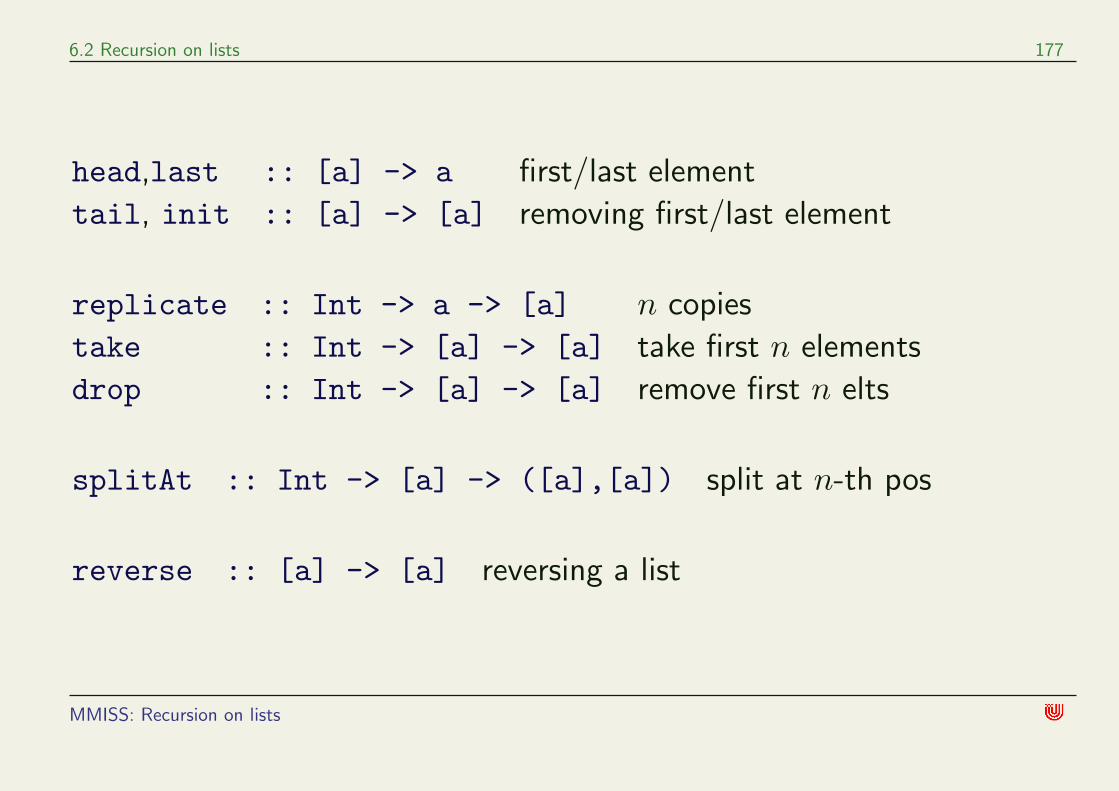
head,last :: [a] -> a first/last element
tail, init :: [a] -> [a] removing first/last element
replicate :: Int -> a -> [a] n copies
take :: Int -> [a] -> [a] take first n elements
drop :: Int -> [a] -> [a] remove first n elts
splitAt :: Int -> [a] -> ([a],[a]) split at n-th pos
reverse :: [a] -> [a] reversing a list
MMISS: Recursion on lists

6.2 Recursion on lists 178
zip :: [a] -> [b] -> [(a,b)] two lists into a
list of pairs
unzip :: [(a, b)] -> ([a], [b]) inverse to zip
and, or :: [Bool] -> Bool conjunction/disjunction
sum :: Num a => [a] -> a sum
product :: Num a => [a] -> a product
Exercise for the lab classes on 5/11 and 6/11:
Define the functions above that haven’t yet been defined in the notes
(use different names in order to avoid name conflicts with the Prelude
library).
MMISS: higher-order list functions

6.3 Higher-order functions on lists 179
6.3 Higher-order functions on lists
• map: Applying a function to all its elements (predefined)
map :: (a -> b) -> [a] -> [b]map f [] = []map f (x:xs) = (f x) : (map f xs)
Informally:
map f [x1, . . . , xn] = [f x1, . . . , f xn]
MMISS: higher-order list functions

6.3 Higher-order functions on lists 180
• Example: Squaring all elements of a list of integers
squareAll :: [Int] -> [Int]squareAll xs = map (^2) xs
or, even shorter,
squareAll = map (^2)
MMISS: higher-order list functions

6.3 Higher-order functions on lists 181
zipWith, a higher-order version of zip
Informally:
zipWith f [x1, . . . , xn] [y1, . . . , yn] = [f x1 y1, . . . , f xn yn]
zipWith :: (a -> b -> c) -> [a] -> [b] -> [c]zipWith f (x:xs) (y:ys) = f x y : zip xs yszipWith _ _ _ = []
zipWith (*) [2,3,4] [7,8,9] [14,24,36]
MMISS: higher-order list functions

6.3 Higher-order functions on lists 182
’Folding’ lists (predefined)
foldr :: (a -> b -> b) -> b -> [a] -> bfoldr f e [] = efoldr f e (x:xs) = f x (foldr f e xs)
Informally:
foldr f e [x1, . . . , xn] = f x1 (f x2 (. . . f xn e) )
or, writing f infix:
foldr f e [x1, . . . , xn] = x1 ‘f ‘ ( x2 ‘f ‘ (. . . ( xn ‘f ‘ e ) ) )
MMISS: higher-order list functions

6.3 Higher-order functions on lists 183
• Defining sum using foldr
sum :: [Int] -> Intsum xs = foldr (+) 0 xs
sum [3,12] = 3 + sum [12]= 3 + 12 + sum []= 3 + 12 + 0 = 15
MMISS: higher-order list functions

6.3 Higher-order functions on lists 184
• Flattening lists using foldr
concat :: [[a]]-> [a]concat xs = foldr (++) [] xs
concat [l1,l2,l3,l4] = l1 ++ l2 ++ l3 ++ l4 ++ []
MMISS: higher-order list functions

6.3 Higher-order functions on lists 185
Taking parts of lists
We had already take, drop.Now we consider similar higher-order functions.
• Longest prefix for which property holds (predefined):
takeWhile :: (a -> Bool) -> [a] -> [a]takeWhile p [] = []takeWhile p (x:xs)
| p x = x : takeWhile p xs| otherwise = []
MMISS: higher-order list functions

6.3 Higher-order functions on lists 186
• Rest of this longest prefix (predefined):
dropWhile :: (a -> Bool) -> [a] -> [a]dropWhile p [] = []dropWhile p x:xs
| p x = dropWhile p xs| otherwise = x:xs
• It holds: takeWhile p xs ++ dropWhile p xs == xs
• Combination of both
span :: (a -> Bool) -> [a] -> ([a],[a])span p xs = (takeWhile p xs, dropWhile p xs)
MMISS: higher-order list functions

6.3 Higher-order functions on lists 187
• Order preserving insertion
ins :: Int-> [Int]-> [Int]ins x xs = lessx ++ [x] ++ grteqx where
(lessx, grteqx) = span (< x) xs
• We use this to define insertion sort
isort :: [Int] -> [Int]isort xs = foldr ins [] xs
Note that
isort [2,3,1] = 2 ‘ins‘ (3 ‘ins‘ (1 ‘ins‘ []))
MMISS: higher-order list functions

6.3 Higher-order functions on lists 188
Exercise
Make the functions ins and isort polymorphic.
ins :: Ord a => a -> [a] -> [a]ins x xs = lessx ++ [x] ++ grteqx where
(lessx, grteqx) = span (< x) xs
isort :: Ord a => [a] -> [a]isort xs = foldr ins [] xs
MMISS: List comprehension

6.4 List comprehension 189
6.4 List comprehension
A schema for functions on lists:
• Select all elements of the given list
• which pass a given test
• and transform them in to a result.
MMISS: List comprehension

6.4 List comprehension 190
Examples:
• Squaring all numbers in a list:
[ x * x | x <- [1..10] ]
• Taking all numbers in a list that are divisible by 3:
[ x | x <- [1..10], x ‘mod‘ 3 == 0 ]
• Taking all numbers in a list that are divisible by 3 and squaring them:
[ x * x | x <- [1..10], x ‘mod‘ 3 == 0]
MMISS: List comprehension

6.4 List comprehension 191
General form
[E |c <- L, test1, ... , testn]
With pattern matching:
addPairs :: [(Int,Int)] -> [Int]addPairs ls = [ x + y | (x, y) <- ls ]
addPairs (zip [1,2,3] [10,20,30]) [11,22,33]
Exercise: use zipWith instead of addPairs and zip.
MMISS: List comprehension

6.4 List comprehension 192
Several generators
[E |c1 <- L1, c2 <- L2, ..., test1, ..., testn ]
All pairings between elements of two lists (cartesian product):
[(x,y) | x <- [1,2,3], y <- [7,9]] [(1,7),(1,9),(2,7),(2,9),(3,7),(3,9)]
[(x,y) | y <- [7,9], x <- [1,2,3]] [(1,7),(2,7),(3,7),(1,9),(2,9),(3,9)]
MMISS: List comprehension
6.4 List comprehension 193
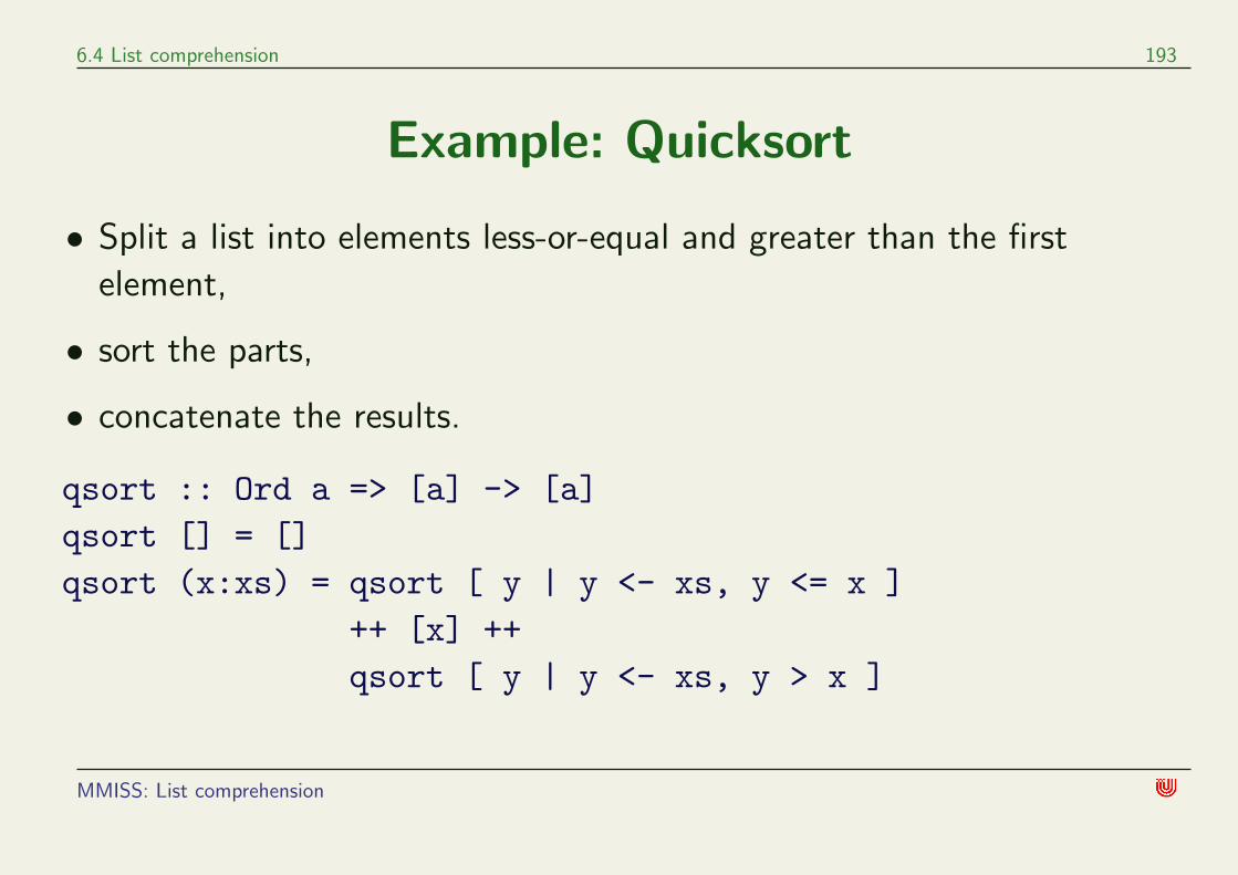
Example: Quicksort
• Split a list into elements less-or-equal and greater than the first
element,
• sort the parts,
• concatenate the results.
qsort :: Ord a => [a] -> [a]qsort [] = []qsort (x:xs) = qsort [ y | y <- xs, y <= x ]
++ [x] ++qsort [ y | y <- xs, y > x ]
MMISS: List comprehension

6.4 List comprehension 194
Filtering elements
filter :: (a -> Bool) -> [a] -> [a]filter p xs = [ x | x <- xs, p x ]
or
filter p [] = []filter p (x:xs)
| p x = x : (filter p xs)| otherwise = filter p xs
MMISS: List comprehension

6.4 List comprehension 195
Exercises
What are the values of the following expressions?
[x | x <- [1..10], x > 5]
[reverse s | s <- ["Hello", "world", "!"]]
Expressing the same using filter and map:
filter (> 5) [1..10]
map reverse ["Hello", "world", "!"]
MMISS: List comprehension

6.4 List comprehension 196
Exercises
• Determine the values of the following expressions (we use the
predefined function even :: Int -> Bool).
map even [1..10]filter even [1..10](sum . filter even) [1..10]
• Define a function that selects from a list of integers all elements that
are even and smaller than 10.
• Define a function that takes a list [x1, x2, ..., xn] and returns
[(x1, x2), (x2, x3), ...(xn−1, xn)].
MMISS: Examples

6.5 Examples 197
6.5 Examples
More examples on programming with lists:
• Shopping baskets
• Modelling a library
• Sorting with ordering as input
• Prime numbers: The sieve of Eratosthenes
• Forward composition
• Computing an Index
MMISS: Examples

6.5 Examples 198
Shopping baskets
• An item consists of a name and a price.
A basket is a list of items.
type Item = (String, Int)type Basket = [Item]
MMISS: Examples

6.5 Examples 199
• The total price of the content of a basket.
total :: Basket -> Inttotal [] = 0total ((name, price):rest) = price + total rest
or
total basket = sum [price | (_,price) <- basket]
MMISS: Examples

6.5 Examples 200
Modelling a library
type Person = Stringtype Book = Stringtype DBase = [(Person, Book)]
MMISS: Examples

6.5 Examples 201
• Borrowing and returning books.
makeLoan :: DBase -> Person -> Book -> DBasemakeLoan dBase pers bk = (pers,bk) : dBase
returnLoan :: DBase -> Person -> Book -> DBasereturnLoan dBase pers bk
= [ pair | pair <- dBase, pair /= (pers,bk) ]
MMISS: Examples

6.5 Examples 202
• All books a person has borrowed.
books :: DBase -> Person -> [Book]books db pers
= [ bk | (p,bk) <- db, p == pers ]
• Exercises
Returning all books.
Finding all persons that have borrowed a book.
Testing whether a person has borrowed any books.
MMISS: Examples

6.5 Examples 203
Sorting with ordering as input
qsortBy :: (a -> a -> Bool) -> [a] -> [a]qsortBy ord [] = []qsortBy ord (x:xs) =
qsortBy ord [y| y <- xs, ord y x] ++ [x] ++qsortBy ord [y| y <- xs, not (ord y x)]
Sorting the library database by borrowers.
sortDB :: DBase -> DBasesortDB = qsortBy (\(p1,_) -> \(p2,_) -> p1 < p2)
MMISS: Examples

6.5 Examples 204
Computing prime numbers
• Sieve of Eratosthenes
When a prime number p is found, remove all multiples of it, that is,
leave only those n for which n ‘mod‘ p /= 0.
sieve [] = []sieve (p:xs) =
p : sieve [n | n <- xs, n ‘mod‘ p /= 0]
• All primes in the interval [1..n]
primes :: Integer -> [Integer]primes n = sieve [2..n]
MMISS: Examples

6.5 Examples 205
Forward composition
• Recall the (predefined) composition operator:
(.) :: (b -> c) -> (a -> b) -> a -> c(f . g) x = f (g x)
• Sometimes it is better to swap the functions:
(>.>) :: (a -> b) -> (b -> c) -> a -> c(f >.> g) x = g (f x)
MMISS: Examples

6.5 Examples 206
• Example: the length of a vector. |[x1, . . . , xn]| =√
(x21 + . . . + x2
n).
len :: [Float] -> Floatlen = (map (^2)) >.> sum >.> sqrt
MMISS: Examples

6.5 Examples 207
Computing an index
• Problem: Given a text
John Anderson my jo, John,\nwhen we were first aquent,\nyour locks were like the raven,\nyour bonnie brow asbent;\nbut now your brow is beld, John,\nyour locks arelike the snow;\nbut blessings on your frosty pow,\nJohnAnderson, my jo. (Robert Burns 1789)
produce for every word the list of lines were it occurs:
[([8],"1789"),([1,8],"Anderson"),([8],"Burns"),([1,1,5,8],"John"),([8],"Robert"),([2],"aquent"),([5],"belt"),([4],"bent"),([7],"blessings"),([4],"bonnie"),([4,5],"brow"),([2],"first"),([7],"frosty"),([3,6],"like"),([3,6],"locks"),([3],"raven"),([6],"snow"),([2,3],"were"),([2],"when"),([3,4,5,6,7],"your")]
MMISS: Examples

6.5 Examples 208
• Specification
type Doc = Stringtype Line = Stringtype Wor = String -- Word predefined
makeIndex :: Doc -> [([Int], Wor)]
MMISS: Examples

6.5 Examples 209
• Dividing the problem into small steps Result type
(a) Split text into lines [Line]
(b) Tag each line with its number [(Int, Line)]
(c) Split lines into words (keeping the line number) [(Int, Wor)]
(d) Sort by words: [(Int,Wor)]
(e) Collect same words with different numbers [([Int], Wor)]
(f) Remove words with less than 4 letters [([Int], Wor)]
MMISS: Examples

6.5 Examples 210
• Main program:
makeIndex :: Doc -> [([Int],Wor)]makeIndex = -- Doc
lines >.> -- [Line]numLines >.> -- [(Int,Line)]numWords >.> -- [(Int,Wor)]sortByWords >.> -- [(Int,Wor)]amalgamate >.> -- [([Int],Wor)]shorten -- [([Int],Wor)]
MMISS: Examples

6.5 Examples 211
• Implementing the parts:
Split into lines: lines :: Doc -> [Line] predefined
Tag each line with its number:
numLines :: [Line] -> [(Int, Line)]numLines ls = zip [1.. length ls] ls
MMISS: Examples

6.5 Examples 212
Split lines into words:
numWords :: [(Int, Line)] -> [(Int, Wor)]Idea: Apply to each line: words:: Line -> [Wor] (predefined).
Problem:
. recognises spaces only
. therefore need to replace all punctuations by spaces
MMISS: Examples

6.5 Examples 213
numWords :: [(Int, Line)] -> [(Int, Wor)]numWords = concat . map oneLine where
oneLine :: (Int, Line) -> [(Int, Wor)]oneLine (num, line) = map (\w -> (num, w))
(splitWords line)
\pagebreak
splitWords :: Line -> [Wor]splitWords line =
words [if c ‘elem‘ puncts then ’ ’ else c | c <- line ]where puncts = ";:.,\’\"!?()-\\[]"
MMISS: Examples

6.5 Examples 214
Sort by words:
sortByWords :: [(Int, Wor)] -> [(Int, Wor)]sortByWords = qsortBy ordWord where
ordWord (n1, w1) (n2, w2) =w1 < w2 || (w1 == w2 && n1 <= n2)
MMISS: Examples

6.5 Examples 215
Collect same words with different numbers
amalgamate :: [(Int, Wor)]-> [([Int],Wor)]amalgamate nws = case nws of
[] -> [](_,w) : _ -> let ns = [ n | (n,v) <- nws, v == w ]
other = filter (\(n,v) -> v /= w) nwsin (ns,w) : amalgamate other
MMISS: Examples

6.5 Examples 216
Remove words with less than 4 letters
shorten :: [([Int],Wor)] -> [([Int],Wor)]shorten = filter (\(_, wd) -> length wd >= 4)
Alternative definition:
shorten = filter ((>= 4) . length . snd)
MMISS:

7 Algebraic data types

7 Algebraic data types 218
Contents
• Simple data
• Composite data
• Recursive data
MMISS: Algebraic data types

7.1 Simple data 219
7.1 Simple data
A simple predefined algebraic data type are the booleans:
data Bool = False | Truederiving (Eq, Show)
• The data type Bool contains exactly the constructors False and True.
• The expression ‘deriving(Eq, Show)’ puts Bool into the type classes
Eq and Show using default implementations of ==, /= and show.
MMISS: Simple data

7.1 Simple data 220
Example: Days of the week
We may also define our own data types:
data Day = Sun | Mon | Tue | Wed | Thu | Fri | Satderiving(Eq, Ord, Enum, Show)
• Ord: Constructors are ordered from left to right
• Enum: Enumeration and numbering
fromEnum :: Enum a => a -> InttoEnum :: Enum a => Int -> a
MMISS: Simple data

7.1 Simple data 221
Wed < Fri TrueWed < Wed FalseWed <= Wed True
max Wed Sat Sat
fromEnum Sun 0
fromEnum Mon 1
fromEnum Sat 6
toEnum 2 ERROR - Unresolved overloading ...toEnum 2 :: Day TuetoEnum 7 :: Day Program error ...
enumFromTo Mon Thu [Mon,Tue,Wed,Thu][(Mon)..(Thu)] [Mon,Tue,Wed,Thu]
MMISS: Simple data

7.1 Simple data 222
Pattern matching
Example: Testing whether a day is a work day
• Using several equations
workDay :: Day -> BoolworkDay Sun = FalseworkDay Sat = FalseworkDay _ = True
MMISS: Simple data

7.1 Simple data 223
• The same function using a new form of definition by cases:
workDay :: Day -> BoolworkDay d = case d of
Sun -> FalseSat -> False_ -> True
MMISS: Simple data

7.1 Simple data 224
• We can also use the derived ordering
workDay :: Day -> BoolworkDay d = Mon <= d && d <= Fri
• or guarded equations
workDay :: Day -> BoolworkDay d
|d == Sat || d == Sun = False|otherwise = True
MMISS: Simple data

7.1 Simple data 225
Example: Computing the next day
• Using enumeration
dayAfter :: Day -> DaydayAfter d = toEnum ((fromEnum d + 1) ‘mod‘ 7)
• The same with the composition operator
dayAfter :: Day -> DaydayAfter = toEnum . (‘mod‘ 7) . (+1) . fromEnum
Exercise: Define dayAfter without mod using case analysis instead.
MMISS: Simple data

7.1 Simple data 226
Summary
• data is a keyword for introducing a new data type with constructors.
• Data types defined in this way are called algebraic data types.
• Names of data types and constructors begin with an upper case letter.
• Definition by cases can be done via pattern matching on constructors.
MMISS: Algebraic data types

7.2 Composite data 227
7.2 Composite data
We use representations of simple geometric shapes as an example for
composite data.
type Radius = Floattype Pt = (Float,Float)
data Shape = Ellipse Pt Radius Radius| Polygon [Pt]
deriving (Eq, Show)
MMISS: Composite data

7.2 Composite data 228
• Ellipse p r1 r2 represents an ellipse with center p and radii r1,r2 (in x-, resp. y-direction).
• Polygon ps represents a polygon with list of corners ps (clockwise
listing).
• For example, Polygon [(-1,-1),(-1,1),(1,1),(1,-1)] represents
a centred square of side length 2.
MMISS: Composite data

7.2 Composite data 229
The type of a constructor
• In a data type declaration
data DataType = Constr Type1 ... Typen | . . .
the type of the constructor is
Constr :: Type1 -> ... -> Typen -> DataType
• In our examples:
True, False :: BoolSun,...,Sat :: DayElipse :: Pt -> Radius -> Radius -> ShapePolygon :: [Pt] -> Shape
MMISS: Composite data

7.2 Composite data 230
Creating circles
A circle with center p and radius r:
circle :: Pt -> Radius -> Shapecircle p r = Ellipse p r r
MMISS: Composite data

7.2 Composite data 231
Creating rectangles
A rectangle is given by its bottom left and top right corner (we list the
corners clockwise).
rectangle :: Pt -> Pt -> Shaperectangle (x,y) (x’,y’) =
Polygon [(x,y),(x,y’),(x’,y’),(x’,y)]
MMISS: Composite data

7.2 Composite data 232
Rotating points
Our next goal is to create a regular polygon with n corners and ‘radius’
r. For this, we need a program that rotates a point around the origin
(anticlockwise).
type Angle = Float
rotate :: Angle -> Pt -> Ptrotate alpha (x,y) = (a*x-b*y,b*x+a*y) where
a = cos alphab = sin alpha
MMISS: Composite data

7.2 Composite data 233
Creating a regular polygon
Creating a centered regular polygon with n corners and one corner at
point p.
regPol :: Int -> Pt -> ShaperegPol n p =
Polygon [rotate (fromIntegral k * theta) p| k <- [0..(n-1)]]
wheretheta = - (2 * pi / fromIntegral n)
MMISS: Composite data

7.2 Composite data 234
Shifting shapes
Shifting a shape:
addPt :: Pt -> Pt -> PtaddPt (x1,y1) (x2,y2) = (x1+x2,y1+y2)
shiftShape :: Pt -> Shape -> ShapeshiftShape p sh = case sh of
Ellipse q r1 r2 -> Ellipse (addPt p q) r1 r2Polygon ps -> Polygon (map (addPt p) ps)
MMISS: Composite data

7.2 Composite data 235
Scaling shapes
scalePt :: Float -> Pt -> PtscalePt z (x,y) = (z * x, z * y)
scaleShape :: Float -> Shape -> ShapescaleShape z sh = case sh of
Ellipse p r1 r2 ->Ellipse (scalePt z p) (z*r1) (z*r2)
Polygon ps -> Polygon (map (scalePt z) ps)
MMISS: Composite data

7.2 Composite data 236
Summary
• Using the data keyword the user can introduce new structured data.
• In a data type declaration
data DataType = Constr Type1 ... Typen | . . .
the type of the constructor is
Constr :: Type1 -> ... -> Typen -> DataType
• Definition by cases on structured data can be done using the caseconstruct. Wild cards (underscores) are allowed.
MMISS: Composite data

7.3 Recursive data 237
7.3 Recursive data
The most common recursive data type is the type of lists:
data [a] = [] | a : [a]
Without using the special infix (and aroundfix) notation the definition of
lists would read as follows:
data List a = Nil | Cons a (List a)
This definition is recursive because the defined type constructor Listoccurs on the right hand side of the defining equation. We will discuss a
few other common examples of recursive data.
MMISS: Composite data

7.3 Recursive data 238
Binary Trees
A binary tree is
• either empty,
• or a node with exactly two subtrees.
• Each node carries an integer as label.
data Tree = Null| Node Tree Int Tree
deriving (Eq, Read, Show)
MMISS: Composite data

7.3 Recursive data 239
Examples of trees
tree0 = Null
tree1 = Node Null 3 Null
MMISS: Composite data

7.3 Recursive data 240
tree2 = Node (Node Null 5 Null)2(Node (Node Null 7 Null)
5(Node Null 1 Null))
tree3 = Node tree2 0 tree2
MMISS: Composite data

7.3 Recursive data 241
Balanced trees
Creating balanced trees of depth n with label indicating depth of node:
balTree :: Int -> TreebalTree n = if n == 0
then Nullelse let t = balTree (n-1)
in Node t n t
MMISS: Composite data
7.3 Recursive data 242
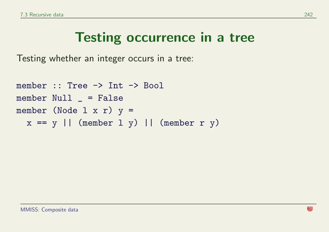
Testing occurrence in a tree
Testing whether an integer occurs in a tree:
member :: Tree -> Int -> Boolmember Null _ = Falsemember (Node l x r) y =
x == y || (member l y) || (member r y)
MMISS: Composite data
7.3 Recursive data 243
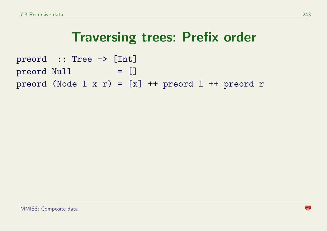
Traversing trees: Prefix order
preord :: Tree -> [Int]preord Null = []preord (Node l x r) = [x] ++ preord l ++ preord r
MMISS: Composite data

7.3 Recursive data 244
Traversing trees: Infix and postfix
Infix and postfix order:
inord :: Tree -> [Int]inord Null = []inord (Node l x r) = inord l ++ [x] ++ inord r
postord :: Tree -> [Int]postord Null = []postord (Node l x r) =
postord l ++ postord r ++ [x]
MMISS: Composite data

7.3 Recursive data 245
Structural recursion
The definitions of member, preorder, inorder, postorder are
examples of
structural recursion on trees
The pattern is:
• Base. Define the function for the empty tree
• Step. Define the function for a composite tree using recursive calls to
the left and right subtree.
MMISS: Composite data

7.3 Recursive data 246
Ordered trees
A tree Node l x r is ordered if
member l y implies y < x and
member r y implies x < y and
l and r are ordered.
MMISS: Composite data

7.3 Recursive data 247
Example:
t = Node (Node (Node Null 1 Null)5
(Node Null 7 Null))9(Node (Node Null 13 Null)
15(Node Null 29 Null))
MMISS: Composite data

7.3 Recursive data 248
Efficient membership test
For ordered trees the test for membership is more efficient:
member :: Tree -> Int -> Boolmember Null _ = Falsemember (Node l x r) y| y < x = member l y| y == x = True| y > x = member r y
MMISS: Composite data

7.3 Recursive data 249
Order preserving insertion
Order preserving insertion of a number in a tree:
insert :: Tree -> Int -> Treeinsert Null y = Node Null y Nullinsert (Node l x r) y| y < x = Node (insert l y) x r| y == x = Node l x r| y > x = Node l x (insert r y)
MMISS: Composite data

7.3 Recursive data 250
Order preserving deletion
More difficult: Order preserving deletion.
delete :: Int -> Tree -> Treedelete y Null = Nulldelete y (Node l x r)
| y < x = Node (delete y l) x r| y == x = join l r| y > x = Node l x (delete y r)
join combines in an order preserving way two trees l,r provided all
labels in l are smaller than those in r.
MMISS: Composite data

7.3 Recursive data 251
join :: Tree -> Tree -> Treejoin t Null = tjoin t s = Node t leftmost s1 where
(leftmost, s1) = splitTree ssplitTree :: Tree -> (Int, Tree)splitTree (Node Null x t) = (x, t)splitTree (Node l x r) =
(leftmost, Node l1 x r) where(leftmost, l1) = splitTree l
MMISS: Composite data

7.3 Recursive data 252
Regions
We define a recursive data type Region that contains shapes as basic
objects and has constructors for rotation and boolean combinations of
regions:
data Region = Sh Shape| Rotate Float Region| Inter Region Region| Union Region Region| Compl Region| Empty
MMISS: Composite data

7.3 Recursive data 253
The meaning of regions
The meaning of a region is a set of points in the 2-dimensional plane.
Therefore, in order to define the meaning of a region, we must decide
when a point lies in the region.
inRegion :: Region -> Pt -> Bool
If we set (as in the 2nd coursework)
type Bitmap = Pt -> Bool
then we have
MMISS: Composite data

7.3 Recursive data 254
inRegion :: Region -> Bitmap
i.e. inRegion transforms a region into a bitmap. which can in turn be
transformed into a picture (see Coursework 2).
For example, a point p is in the region
Union reg1 reg2
if and only if it is in reg1 or in reg2.
MMISS: Composite data

7.3 Recursive data 255
Examples of regions
A ring with outer radius 1.5 and inner radius 1:
ring = Inter (Sh (circle (0,0) 1.5))(Compl (Sh (circle (0,0) 1)))
A tree:
tree = Union (Sh (rectangle (-0.2,-1) (0.2,0.6)))(Sh (circle (0,1) 0.5))
MMISS: Composite data

7.3 Recursive data 256
Operations on Regions
Shifting:
shiftRegion :: Pt -> Region -> Region
shiftRegion p (Sh sh) = Sh (shiftShape p sh)
shiftRegion p (Union reg1 reg2) = Union (shiftRegion p reg1)(shiftRegion p reg2)
shiftRegion p (Inter reg1 reg2) = Inter (shiftRegion p reg1)(shiftRegion p reg2)
MMISS: Composite data

7.3 Recursive data 257
shiftRegion p (Compl reg) = Compl (shiftRegion p reg)
shiftRegion _ Empty = Empty
The union of a list of regions:
unionRegions :: [Region] -> Region
unionRegions = foldr Union Empty
MMISS: Composite data

7.3 Recursive data 258
Summary
• Using the data keyword the user can introduce new recursive data
types
• Common recursive data types are lists and trees.
• Functions on recursive data types can be defined by structural
recursion. For example, recursion on lists, trees.
• Maintaining special properties of recursive data can lead to efficient
code. Example: membership for ordered trees.
MMISS: Composite data

7.3 Recursive data 259
Exercises
• Compute the circumference of a shape.
• Compute the area of a shape. Hint: see Hudak, page 33.
• Compute the number of corners of a shape.
• Compute the height (or depth) of a tree.
MMISS:

8 Proofs

8 Proofs 261
Contents
• Verifying recursive programs by induction
• Timing analysis
MMISS: Proofs

8.1 Verifying recursive programs by induction 262
8.1 Verifying recursive programs by induction
• Properties of recursive programs can often be proved by a suitable
induction principle.
• Which induction principle is to be applied depends on the underlying
data types.
• In the following we discuss
induction on natural numbers;
induction on lists;
induction on trees.
MMISS: Recursion induction

8.1 Verifying recursive programs by induction 263
Induction on natural numbers
• In order to prove
for all natural numbers n, property P (n) holds
• one needs to prove
induction base: P (0)
induction step: assuming P (n), show P (n + 1).
Remark: The assumption P (n) in the induction step is usually called
induction hypothesis, abbreviated i.h..
MMISS: Recursion induction

8.1 Verifying recursive programs by induction 264
• Example:
f :: Int -> Intf n = if n == 0 then 0 else f (n-1) + n
Show that for all natural numbers n (that is, integers n ≥ 0) the
equation f n = n∗(n+1)2 holds.
Base: f 0 = 0 = 0∗(0+1)2 .
Step: Assume f n = n∗(n+1)2 (i.h.).
We have to show f (n + 1) = (n+1)∗(n+2)2 .
f (n + 1) = f n + (n + 1) i.h.=n ∗ (n + 1)
2+ n + 1 =
=n ∗ (n + 1) + 2 ∗ (n + 1)
2=
(n + 1) ∗ (n + 2)2
MMISS: Recursion induction

8.1 Verifying recursive programs by induction 265
Induction on lists
• In order to prove
for all finite lists xs, property P (xs) holds
• one needs to prove
induction base: P ([])
induction step: assuming P (xs), show P (x : xs) holds for all x.
Here P (xs) is the induction hypothesis.
MMISS: Recursion induction

8.1 Verifying recursive programs by induction 266
• Example:
(++) :: [a] -> [a] -> [a][] ++ ys = ys(x:xs) ++ ys = x : (xs ++ ys)
Show that (++) is associative, that is the equation
(xs ++ ys) ++ zs = xs ++ (ys ++ zs)
holds for all xs,ys,zs.
We prove this by list induction on xs.
MMISS: Recursion induction

8.1 Verifying recursive programs by induction 267
Base: ([] ++ ys) ++ zs = ys ++ zs = [] ++ (ys ++ zs).
Step: Assume (xs ++ ys) ++ zs = xs ++ (ys ++ zs) (i.h.).
We have to show
((x:xs) ++ ys) ++ zs = (x:xs) ++ (ys ++ zs)
for all x.
((x:xs) ++ ys) ++ zs= (x : (xs ++ ys)) ++ zs (by def. of (++))= x : ((xs ++ ys) ++ zs) (by def. of (++))= x : (xs ++ (ys ++ zs)) (by i.h.)= (x:xs) ++ (ys ++ zs) (by def. of (++))
MMISS: Recursion induction

8.1 Verifying recursive programs by induction 268
• Exercises
Prove xs ++ [] = xs
Recall
length :: [a] -> Intlength [] = 0length (x : xs) = 1 + length xs
Prove length (xs ++ ys) = length xs + length ys.
MMISS: Recursion induction

8.1 Verifying recursive programs by induction 269
Consider the function
reverse :: [a] -> [a]reverse [] = []reverse (x : xs) = reverse xs ++ [x]
Prove reverse (xs ++ ys) = reverse ys ++ reverse xs.
MMISS: Recursion induction

8.1 Verifying recursive programs by induction 270
Induction on trees
data Tree a = Null| Node (Tree a) a (Tree a)
• In order to prove
for all finite trees xt, property P (xt) holds
• one needs to prove
induction base: P (Null)
induction step: assuming P (xt) and P (yt), show P (Node xt x yt)holds for all x.
Here we have two induction hypotheses: P (xt) and P (yt).
MMISS: Recursion induction

8.1 Verifying recursive programs by induction 271
• Example:
height :: Tree a -> Intheight Null = 0height Node xt _ yt = 1 + max (height xt) (height yt)
preord :: Tree a -> [a]preord Null = []preord (Node xt x yt) = [x] ++ preord xt ++ preord yt
Show
length (preord xt) <= 2^(height xt) - 1
holds for all trees xt.
We prove this by tree induction:
MMISS: Recursion induction

8.1 Verifying recursive programs by induction 272
• Base:
length (preord Null) = length [] = 0 = 2^(height Null) - 1.
• Step: Assume
length (preord xt) <= 2^(height xt) - 1
and
length (preord yt) <= 2^(height yt) - 1 (i.h.).
We have to show
length(preord(Node xt x yt)) <= 2^(height(Node xt x yt))-1
for all x.
MMISS: Recursion induction

8.1 Verifying recursive programs by induction 273
length (preord (Node xt x yt))= length ([x] ++ preord xt ++ preord yt) (def. preord)
= 1 + length(preord xt) + length(preord yt)
<= 1 + 2^(height xt) - 1 + 2^(height yt) - 1 (by i.h.)
= 2^(height xt) + 2^(height yt) - 1
<= 2 * 2^(max (height xt) 2^(height yt)) - 1
= 2^(1 + max (height xt) (height yt)) - 1
<= 2^(height (Node xt x yt)) - 1 (def. height)
MMISS: Proofs

8.2 Timing analysis 274
8.2 Timing analysis
• The run-time of an expression is measured in terms of the number of
reduction steps necessary to evaluate it.
• The run-time of a function f is the asymptotic behaviour of the
runtime of f x depending on the size of x.
• Asymptotic behaviour is expressed mathematically by the ‘big Oh-’
and similar notations (Algorithms & Complex.).
• In the following we discuss
the run-times of recursive functions on lists and trees;
evaluation strategy dependent run-times (lazy vs. eager).
MMISS: Timing analysis

8.2 Timing analysis 275
Run-times of functions on lists
• We define the size of a list xs as its length.
• Example: To compute xs ++ ys takes n + 1 reduction steps where n
is the length of xs.
Proof by list induction on xs:
Base: [] ++ ys ys (one reduction)
Step: Assume computing xs ++ ys needs n + 1 reductions.
We have to show (x:xs) ++ ys needs n + 2 reductions:
(x:xs) ++ ys x:(xs ++ ys) in n + 1 steps to value.
• Therefore (++) has run-time complexity O(n).
MMISS: Timing analysis

8.2 Timing analysis 276
• Example: Our program for reversing list has run-time complexity
O(n2).
Proof: We show by list induction that evaluation of reverse xs needs
n ∗ (n + 3)2
+ 1
reductions, where n is the length of the list.
Base:
reverse [] [] (one step).
0 ∗ (n + 3)2
+ 1 = 1
MMISS: Timing analysis

8.2 Timing analysis 277
Step:
reverse (x : xs) reverse xs ++ [x].
By i.h. reverse xs needs n∗(n+3)2 + 1 steps.
It is easy to see that reverse xs has length n (Exercise).
Hence, by the previous result on (++) the total number of steps is
1 + (n ∗ (n + 3)
2+ 1) + (n + 1) = . . . =
(n + 1) ∗ (n + 4)2
+ 1
MMISS: Timing analysis

8.2 Timing analysis 278
• Recall the linear program for reversing lists:
reverse1 :: [a] -> [a]reverse1 xs = revConc xs []
revConc :: [a] -> [a] -> [a]revConc [] ys = ysrevConc (x:xs) ys = revConc xs (x:ys)
It is easy to prove that the function revConc has run-time complexity
O(n) (Exercise) and
reverseConc xs ys = reverse xs ++ ys (Exercise).
MMISS: Timing analysis

8.2 Timing analysis 279
Run-times of functions on trees
• We define the size of a tree as the number of its nodes.
• Example: To compute preord xt takes O(n2) steps where n is the
size of the tree xt
• Exercise: Prove this!
MMISS: Timing analysis

8.2 Timing analysis 280
• A linear program for preord (using a similar idea as in the linear
implementation of reverse):
preord :: Tree a -> [a]preord xt = preConc xt [] wherepreConc Null zs = zspreConc (Node xt x yt) zs =
x : preConc xt (preConc yt zs)
It easy to prove that the function preConc has run-time complexity
O(n) (Exercise).
MMISS: Timing analysis

8.2 Timing analysis 281
Lazy evaluation versus eager evaluation
• Recall that Haskell applies a lazy evaluation strategy: Subexpressions
are reduced only when their value is needed. This strategy is achieved
by outermost reduction, which means reduction takes place as close to
the root of the expression as possible.
• Another reduction strategy is eager evaluation which is achieved by
innermost reduction, i.e. reduction takes place as close to the leaves of
the expression as possible.
• Most programming languages apply eager evaluation (e.g. ML, Lisp,
Java,. . . ).
MMISS: Timing analysis

8.2 Timing analysis 282
• None of the strategies outperforms the other in general.
• But, lazy evaluation is safe concerning termination: When an
expression terminates by some strategy, then it also terminates with
lazy evaluation.
• In the previous examples of timing analysis the evaluation strategy did
not matter.
• In the following example the strategy does matter.
MMISS: Timing analysis

8.2 Timing analysis 283
• Computing the first n labels of a tree in prefix order:
takeTree :: Int -> Tree a -> [a]takeTree n xt = take n (preord xt)
take :: Int -> [a] -> [a]take n _ | n <= 0 = []take _ [] = []take n (x:xs) = x : take (n-1) xs
Applying lazy evaluating this program has time complexity O(n).
Note that the complexity is independent of xt !
MMISS: Timing analysis

8.2 Timing analysis 284
For example
takeTree 1 (Node xt x yt)
take 1 (preord (Node xt x yt))
take 1 ([x] ++ preord xt ++ preord yt)
take 1 (x : (preord xt ++ preord yt))
x : take 0 (preord xt ++ preord yt) [x]
• With eager evaluation the time complexity would be O(max(n, m))where m is the size of xt, because preord xt would be evaluated
completely first.
MMISS: Timing analysis

8.2 Timing analysis 285
Summary and concluding remarks
• In functional programming functions are defined by equations which
can be used to apply rigorous reasoning to prove properties of
programs
• Important and useful proof principles are induction on numbers, lists
and trees.
MMISS: Timing analysis

8.2 Timing analysis 286
• Timing analysis can be done by counting reductions.
• The reduction strategy can have an impact on the run-time complexity.
MMISS: Timing analysis

8.2 Timing analysis 287
Exercises
• Prove length (filter p xs) =< length xs.
• Prove map (f . g) xs = map f (map g xs),
recalling that (f . g) x = f (g x).
MMISS: Timing analysis

8.2 Timing analysis 288
• Prove length (reverse xs) = length xs.
• Prove reverseConc xs ys = reverse xs ++ ys and conclude
form this the correctness of the function reverse1, that is,
reverse1 xs = reverse xs.
MMISS:

9 Abstract Data Types

9 Abstract Data Types 290
Contents
• The concept of an Abstract Data Type (ADT)
• Implementation of ADTs by modules
• The ADT of Sets
• Minimality vs. efficiency
MMISS: Abstract data types

9.1 The concept of an Abstract Data Type 291
9.1 The concept of an Abstract Data Type
• An Abstract Data Type (ADT) consists of a bunch of data types and
functions.
• An ADT has a precise interface (also called signature) describing the
available data types and function.
• Details of how data are constructed and functions are defined may be
hidden.
• The main advantage of an ADT is that its implementation may be
changed without affecting the validity of programs using the ADT.
MMISS: Modules

9.2 Implementation of ADTs by modules 292
9.2 Implementation of ADTs by modules
• A module consists of:
Definitions of types, functions, classes
Declaration of the definitions that are visible from outside (interface,
signature).
• Syntax:
module Name (visible names) where body
visible names may be empty
• The main idea behind modules is to control visibility by encapsulation.
MMISS: Modules

9.2 Implementation of ADTs by modules 293
Example: Storage (Store)
• Type of storage parametrised by index (or address) type a and value
type b.
Store a b
• Empty storage: initial :: Store a b
• Reading a value:
value :: Eq a => Store a b -> a -> Maybe b
Uses data Maybe b = Nothing | Just b
• Writing:
update :: Eq a => Store a b -> a -> b -> Store a b
• Module declaration (interface)
MMISS: Modules

9.2 Implementation of ADTs by modules 294
module Store(Store,initial, -- :: Store a bvalue, -- :: Eq a => Store a b -> a -> Maybe bupdate, -- :: Eq a => Store a b -> a -> b -> Store a b) where
(Signature not necessary, but helpful)
MMISS: Modules

9.2 Implementation of ADTs by modules 295
• Body of module: Implementation of storage as a list of pairs
type Store a b = [(a, b)]
initial :: Store a binitial = []
MMISS: Modules

9.2 Implementation of ADTs by modules 296
value :: Eq a => Store a b -> a -> Maybe bvalue ls a =
case [b | (x,b) <- ls, a == x] ofb : _ -> Just b[] -> Nothing
update :: Eq a => Store a b -> a -> b ->Store a b
update ls a b = (a, b) : ls
MMISS: Modules

9.2 Implementation of ADTs by modules 297
• The complete code for the module (interface + body) must be written
in the file Store.hs (capital S!).
• The ADT Store is also known under the name Map.
• Note that nothins is exported that would reveal that we have
implemented stores via lists. This is important since it gives us the
possibility to change the implementation of the ADT Store without
changing its interface.
MMISS: Importing a module

9.2 Implementation of ADTs by modules 298
Importing a module
• import Name (identifiers)
The identifiers declared in module Name are imported.
If (identifiers) is omitted, then everything is imported.
• Example: The line
import Store
imports everything from the interface of the module Store, that is,
the data type Store and the functions initial, value, update.
MMISS: Using Store

9.2 Implementation of ADTs by modules 299
Using the ADT Store
Storing the values x0,x1,...,xn
at the addresses k,k+1,...,k+n.
import Store (Store, initial, value, update)
mkStore :: [a] -> Int -> Store Int amkStore [] k = initialmkStore (x:xs) k = update (mkStore xs (k+1)) k x
MMISS: Modules

9.2 Implementation of ADTs by modules 300
Reimplementing the ADT Store usingfunctions
type Store a b = a -> Maybe b
initial :: Store a binitial = \_ -> Nothing
value :: Eq a => Store a b -> a -> Maybe bvalue f a = f a
MMISS: Modules

9.2 Implementation of ADTs by modules 301
update :: Eq a => Store a b -> a -> b ->Store a b
update f a b= \x -> if x == a then Just b else f x
MMISS: Sets

9.3 The ADT of Sets 302
9.3 The ADT of Sets
In the following we discuss the important ADT of sets in some detail.
Common requirements on a data type of sets are:
1. There is an empty set: ∅
2. We can insert an element in a set: x ∪ s
3. We can test if an element is a member of a set: x ∈ s
4. We can compute the union of two sets: s ∪ t
5. Filtering: Given a set s and a property p of elements we can compute
a set containing exactly those members of s that have property p:
x ∈ s | p(x) = True
MMISS: Sets

9.3 The ADT of Sets 303
6. Extensionality: Two sets s, t are equal when they contain the same
elements, that is, an element is a member of s if and only if it is a
member of t:
s = t ⇐⇒ ∀x(x ∈ s↔ x ∈ t)
We do not (yet) require a test for deciding equality of sets.
MMISS: Sets

9.3 The ADT of Sets 304
Implementation of sets
• As type of elements of sets we admit any type a that has an equality
test (i.e. a must be an instance of the class Eq).
• We will begin with a discussion of two implementations of sets:
(a) Sets as boolean functions.
(b) Sets as lists of elements.
MMISS: Sets

9.3 The ADT of Sets 305
Sets – Interface
module Set (Set, -- type constructorempty, -- Set ainsert, -- Eq a => a -> Set a -> Set amember, -- Eq a => a -> Set a -> Boolunion, -- Eq a => Set a -> Set a -> Set asfilter -- Eq a => (a -> Bool) -> Set a -> Set a) where
MMISS: Sets

9.3 The ADT of Sets 306
Implementing sets as boolean functions
type Set a = a -> Bool
empty :: Set aempty = \x -> False
insert :: Eq a => a -> Set a -> Set ainsert x p = \y -> y == x || p y
member :: Eq a => a -> Set a -> Boolmember x p = p x
MMISS: Sets

9.3 The ADT of Sets 307
union :: Eq a => Set a -> Set a -> Set aunion p q = \x -> p x || q x
sfilter :: Eq a => (a -> Bool) -> Set a -> Set asfilter test p = \x -> p x && test x
MMISS: Sets

9.3 The ADT of Sets 308
Implementing sets as lists
type Set a = [a]
empty :: Set aempty = []
insert :: Eq a => a -> Set a -> Set ainsert x xs = x : xs
member :: Eq a => a -> Set a -> Bool
MMISS: Sets

9.3 The ADT of Sets 309
member x xs = elem x xs
union :: Eq a => Set a -> Set a -> Set aunion xs ys = xs ++ ys
sfilter :: Eq a => (a -> Bool) -> Set a -> Set asfilter test xs = filter test xs
MMISS: Sets

9.3 The ADT of Sets 310
Using the ADT Set
import Set (Set, empty, insert, member, union, sfilter)
singleton :: Eq a => a -> Set asingleton x = insert x empty
delete :: Eq a => a -> Set a -> Set adelete x s = sfilter (/= x) s
MMISS: Sets

9.3 The ADT of Sets 311
meet :: Eq a => Set a -> Set a -> Set ameet s t = sfilter (‘member‘ s) t
minus :: Eq a => Set a -> Set a -> Set aminus s t = sfilter (\x -> not (x ‘member‘ t)) s
unions :: Eq a => [Set a] -> Set aunions = foldr union empty
listToSet :: Eq a => [a] -> Set alistToSet xs = foldr insert empty xs
MMISS: Sets

9.3 The ADT of Sets 312
Extending the ADT Set
• Can we define infinite sets, in particular a universal set that contains
all elements of type a?
• Can we compute the complement of a set?
• Easy with the implementation based on boolean functions:
universal :: Set auniversal = \x -> True
complement :: Set a -> Set acomplement p = not . p
• None of these are possible with sets implemented by lists.
MMISS: Sets

9.3 The ADT of Sets 313
• Can we
test whether a set is empty?
compute the number of elements of a set?
decide inclusion/equality between sets?
• The implementation based on boolean functions inhibits the definition
of any of these operations.
• On the other hand there are no problems with the list implementation:
MMISS: Sets

9.3 The ADT of Sets 314
isEmpty :: Set a -> BooleisEmpty xs = case xs of
[] -> True_:_ -> False
card :: Eq a => Set a -> Intcard xs = length (removeDuplicates xs)
removeDuplicates :: Eq a => [a] -> [a]removeDuplicates [] = []removeDuplicates (x:xs)
= (if x ‘elem‘ ys then [] else [x]) ++ yswhere ys = removeDuplicates xs
MMISS: Sets

9.3 The ADT of Sets 315
subset :: Eq a => Set a -> Set a -> Boolsubset [] ys = Truesubset (x:xs) ys = x ‘elem‘ ys && sub xs ys
eqset :: Eq a => Set a -> Set a -> Booleqset s t = s ‘subset‘ t && t ‘subset‘ s
MMISS: Sets

9.3 The ADT of Sets 316
In the following we work with the implementation of Set based on lists.
• Can we list the members of a set?
First attempt:
setToList :: Eq a => Set a -> [a]setToList xs = removeDuplicates xs
Does not work because equality of sets is not respected:
setToList [1,2] [1,2]setToList [2,1] [2,1]
MMISS: Sets

9.3 The ADT of Sets 317
• The problem can be solved, if there is an order on elements:
setToList :: Ord a => Set a -> [a]setToList xs = qsort (removeDuplicates xs)
If we use only ordered and repetition-free lists as representations of
sets, then we can simply define:
setToList :: Ord a => Set a -> [a]setToList xs = xs
MMISS: Modules

9.4 Minimality versus Efficiency 318
9.4 Minimality versus Efficiency
• The interface of our first ADT of sets was minimal in the sense that
we omitted a function if it could be defined by other functions (for
example singleton, delete, meet, minus were defined in this way).
• The advantage of minimal declarations is that less work needs to be
done when the implementation of the module is changed.
• But often functions can be implemented more efficiently by making
direct use of the representation of sets. In this case it is advantageous
to include these functions in the interface of the ADT.
MMISS: Modules

9.4 Minimality versus Efficiency 319
• For example, our definition of meet has time complexity O(n2), but if
sets are represented by ordered lists one can achieve linear time:
meet1 :: Ord a => [a] -> [a] -> [a]meet1 [] _ = []meet1 _ [] = []meet1 (x:xs) (y:ys)|x < y = meet1 xs (y:ys)|x == y = x : meet1 xs ys|x > y = meet1 (x:xs) ys
MMISS: Modules

9.4 Minimality versus Efficiency 320
Without ordering:
meet2 :: Eq a => [a] -> [a] -> [a]meet2 xs ys = [x | x <- xs, x ‘elem‘ ys]
-- meet1 [1,3..10000] [2,4..10000]-- meet2 [1,3..10000] [2,4..10000]
• The implementation of sets as lists, or ordered lists is simple, but
unsuitable for representing large finite sets. If one uses so-called
‘AVL-tree’ for representing sets, then membership test, as well as
insertion and deletion of elements can be performed in logarithmic
time (as opposed to linear time in the implementation with lists).
• AVL-trees are special (almost) balanced ordered trees. They are
discussed in any standard textbook on data structures.
MMISS: Modules

9.4 Minimality versus Efficiency 321
Summary
• An abstract data type (ADT) consists of one or more data types
together with some functions. Details of how data are constructed and
functions are defined are hidden.
• Abstract data types support modularization and make code more
robust: The implementation of an ADT may change without other
programs using it being affected.
• An important abstract data type is the ADT of sets. Sets can be
represented in different ways allowing for implementations of different
operations.
• The choice of representation of may also affect the efficiency of set
operations.
MMISS: Modules

9.4 Minimality versus Efficiency 322
Exercises
• Implement the operations ‘set difference’, ‘powerset’, ‘set inclusion
test’ and ‘set disjointness test’ with sets represented by lists.
• Does an ordering help improving efficiency?
• Estimate the (time) complexities of your implementations.
• Which of the operations above can be implemented with sets
represented as boolean functions?
MMISS:

10 Input/Output

10 Input/Output 324
Contents
• Input/Output in functional languages
• Communication with files
• Actions as values
• Random numbers
MMISS: Input/Output

10.1 Input/Output in functional languages 325
10.1 Input/Output in functional languages
• Problem: Functions with side effects are not referentially transparent
(that is, not all parameters the function depends on are visible).
for example readString :: () -> String ??
• Solution:
Side effects are marked by IO — actions
Actions can be combined with actions only
”once IO, always IO“
MMISS: Input/Output

10.1 Input/Output in functional languages 326
The type IO a
• IO a is the type of actions returning a value of type a when executed.
• The value returned by an action can be used in the next action.
• Two actions are combined by the operator
(>>=) :: IO a -> (a -> IO b) -> IO b
MMISS: Input/Output

10.1 Input/Output in functional languages 327
Actions as an abstract data type
MMISS: Input/Output

10.1 Input/Output in functional languages 328
• If we are given
action1 :: IO a
action2 :: a -> IO b
then the action
action1 >>= action2 :: IO b
first does action1 and then action2 x where x is the value returned
by action1.
MMISS: Input/Output

10.1 Input/Output in functional languages 329
Some predefined actions (Prelude)
• Reading a line from stdin (standard input):
getLine :: IO String
• Writing string to stdout (standard output):
putStr :: String -> IO ()
• Writing string to stdout and inserting a new line:
putStrLn :: String -> IO ()
MMISS: Input/Output

10.1 Input/Output in functional languages 330
A simple example
• Echo:
echo :: IO ()echo = getLine >>= putStrLn >>= \_ -> echo
• Reversed echo:
ohce :: IO ()ohce = getLine >>= putStrLn . reverse >> ohce
where (>>) is predefined:
(>>) :: IO a -> IO b -> IO bf >> g = f >>= \_ -> g
MMISS: Input/Output

10.1 Input/Output in functional languages 331
The meaning of f >> g is
“First do f, then g,
throwing away the value returned by f”.
MMISS: Input/Output

10.1 Input/Output in functional languages 332
The do-notation
• Syntactic sugar for IO:
echo =getLine>>= putStrLn>> echo
⇐⇒
echo =do s <- getLine
putStrLn secho
• Layout: Be careful with indentation in a do construction.
MMISS: Input/Output

10.1 Input/Output in functional languages 333
Example: A simple notebook
A simple notebook using the ADT Store.
• Updating: u <Name> <Value>
• Looking up a value: v <Name>
Note that the only way to modify and use the storage is via the functions
update and value provided by the ADT Store.
MMISS: Input/Output

10.1 Input/Output in functional languages 334
import Store
notebook :: IO ()notebook = loop initial whereloop :: Store String String -> IO ()loop st =do s <- getLine
case words s of"u":name:value:_ -> loop (update st name value)"v":name:_ ->
do putStrLn (case value st name ofJust val -> valNothing -> "Unknown: "++name)
loop st_ -> return ()
MMISS: Input/Output

10.2 Communication with files 335
10.2 Communication with files
• In Prelude predefined:
Writing into files (override, append):
type FilePath = StringwriteFile :: FilePath -> String -> IO ()appendFile :: FilePath -> String -> IO ()
Reading a file (lazy):
readFile :: FilePath -> IO String
MMISS: Input/Output
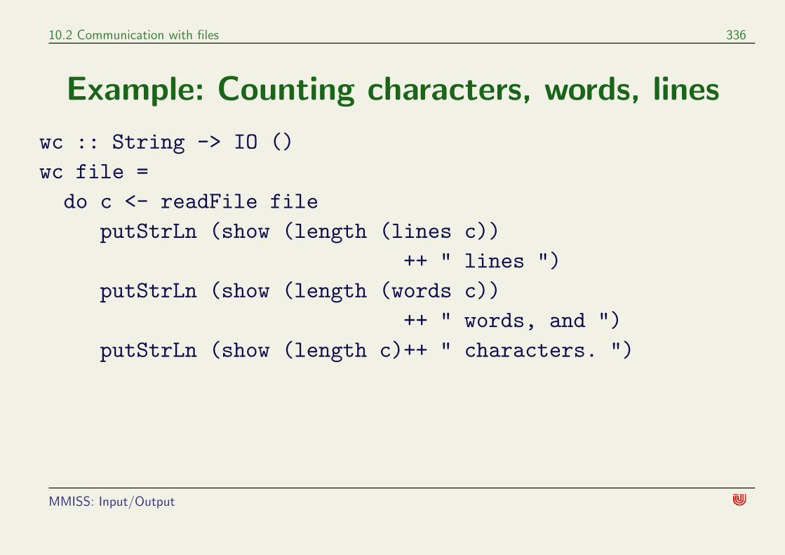
10.2 Communication with files 336
Example: Counting characters, words, lines
wc :: String -> IO ()wc file =
do c <- readFile fileputStrLn (show (length (lines c))
++ " lines ")putStrLn (show (length (words c))
++ " words, and ")putStrLn (show (length c)++ " characters. ")
MMISS: Input/Output

10.3 Actions as values 337
10.3 Actions as values
• Actions are normal values.
• This makes the definition of control structures very easy.
• Better than any imperative language.
MMISS: Input/Output

10.3 Actions as values 338
Predefined control structures (Prelude)
• Sequencing a list of actions:
sequence :: [IO a] -> IO [a]sequence (c:cs) = do x <- c
xs <- sequence csreturn (x:xs)
sequence [act1,...,actn] is the action that does the actions
act1, ..., actn (in that order) and returns the list of results.
MMISS: Input/Output

10.3 Actions as values 339
• Special case: [()] as ()
sequence_ :: [IO ()] -> IO ()
MMISS: Input/Output

10.4 Random numbers 340
10.4 Random numbers
• Example of actions as values: Random numbers.
Module Random, class Random
class Random a whererandomRIO :: (a,a) -> IO arandomIO :: IO a
• For example, randomRIO (0,36) is the action that returns a random
number between 0 and 36.
• Random further contains
Random generators for pseudo random numbers
Infinite lists of random numbers
MMISS: Input/Output

10.4 Random numbers 341
Example: Random words
• Repeating an action a random number of times:
atmost :: Int -> IO a -> IO [a]atmost most a =
do l <- randomRIO (1, most)sequence (replicate l a)
• Random string:
randomStr :: IO StringrandomStr = atmost 10 (randomRIO (’a’,’z’))
MMISS: Input/Output
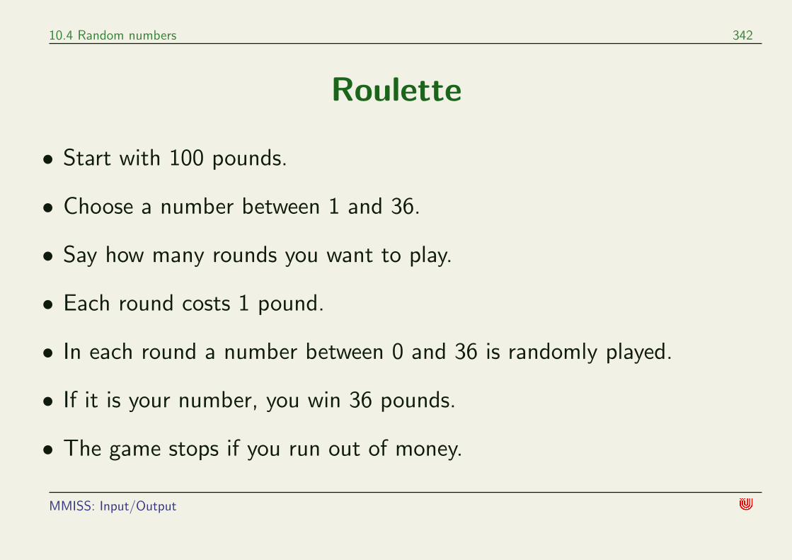
10.4 Random numbers 342
Roulette
• Start with 100 pounds.
• Choose a number between 1 and 36.
• Say how many rounds you want to play.
• Each round costs 1 pound.
• In each round a number between 0 and 36 is randomly played.
• If it is your number, you win 36 pounds.
• The game stops if you run out of money.
MMISS: Input/Output

10.4 Random numbers 343
We use a variant of until that accepts a next function with side effects:
untilIO :: (a -> Bool) -> (a -> IO a) -> a -> IO auntilIO stop next x =
if stop xthen return xelse do x1 <- next x
untilIO stop next x1
Compare this with
until :: (a -> Bool) -> (a -> a) -> a -> auntil stop next x =
if stop xthen xelse let x1 = next x
in until stop next x1
MMISS: Input/Output

10.4 Random numbers 344
import Random (randomRIO)
roulette :: IO ()roulette =
do putStr "You have 100 pounds. Which number do you choose? "n <- getLineputStr "How many rounds do you want to play maximally? "r <- getLinelet mine = read n :: Int
maxRounds = read r :: Intstop (k,money) = k >= maxRounds || money <= 0next (k,money) = do x <- randomRIO (0,36)
let win = if x == mine then 36 else 0return (k+1, money - 1 + win)
(rounds,endMoney) <- untilIO stop next (0,100)putStr ("\nYou played "++(show rounds)++" rounds " ++
"and have now "++(show endMoney)++" pounds")
MMISS: Input/Output

10.4 Random numbers 345
Summary
• Input/Output in Haskell by Actions
Actions (type IO a) are functions with side effects
Combination of actions by
(>>=) :: IO a -> (a -> IO b) -> IO breturn :: a -> IO a
do-Notation
• Various functions from the standard library:
Prelude: getLine, putStr, putStrLn, writeFile, readFile
Modules: IO, Random,
MMISS: Input/Output

10.4 Random numbers 346
• Actions are normal values.
• Useful combinators for actions:
sequence :: [IO a] -> IO [a]
sequence_ :: [IO ()] -> IO ()
untilIO :: (a -> Bool) -> (a -> IO a) -> a -> IO a
MMISS: Input/Output

10.4 Random numbers 347
Exercises
• Write an interactive translation program, say from English to French
and vice versa. Use a dictionary of the form
[(apple,pomme),(street,rue),(sun,soleil),...].
• Modify the program saveCW such that the statistical data are written
to the file as well.
• Modify the program roulette such that after each 100 rounds the
player is informed about their current account and given the choice
whether or not to continue.
MMISS:

11 Infinite lists

11 Infinite lists 349
Contents
• Lazy infinite lists
• Programming with infinite lists
• Corecursion
MMISS: Infinite-lists

11 Infinite lists 350
Lazy infinite lists
Using recursion one can create an infinite list:
ones :: [Int]ones = 1 : ones
Unfolding the definition one obtains
ones = 1 : ones= 1 : 1 : ones= 1 : 1 : 1 : ones= 1 : 1 : 1 : 1 : ones...
Hence ones is an infinite list of 1s.
ones = [1,1,1,1, ...]
MMISS: Infinite-lists

11 Infinite lists 351
Although it is impossible to compute (and print) the complete list onesone can compute parts of it
head ones = head (1 : ones) = 1
Note that due to the lazy evaluation strategy the right occurrence of
ones is not evaluated.
Infinite lists are often called streams.
MMISS: Infinite-lists

11 Infinite lists 352
iterate: iterating a function arbitrarily often
In Haskell’s Prelude we find the following higher-order function:
iterate :: (a -> a) -> a -> [a]iterate f x = x : iterate f (f x)
Unfolding the definition results in
iterate f x = x : iterate f (f x)= x : f x : iterate f (f (f x))= x : f x : f (f x) : iterate f (f (f (f x)))...
MMISS: Infinite-lists

11 Infinite lists 353
For example
iterate (+3) 0 = 0 : iterate (+3) 3= 0 : 3 : iterate (+3) 6= 0 : 3 : 6 : iterate (+3) 9...
Hence
iterate (+3) 0 = [0,3,6,9,...]
take 5 (iterate (+3) 0 = [0,3,6,9,12]
The same stream can be obtained by
= [0,3..]
MMISS: Infinite-lists

11 Infinite lists 354
The lazy Fibonacci numbers
Recall
fib :: Integer -> Integerfib n
| n < 0 = error "negative argument"| n == 0 || n == 1 = 1| n > 0 = fib (n - 1) + fib (n - 2)
We want to compute efficiently the infinite list of Fibonacci numbers
fibs = [fib 0, fib 1, fib 2, fib 3, ... ]= [1,1,2,3,5,8,13,21,34,55, ... ]
MMISS: Infinite-lists

11 Infinite lists 355
Here is how one finds a recursive definition of fibs.
fibs = [1 , 1 , 2 , 3 , 5 , 8 , 13 , ... ]= 1 : 1 :[2 , 3 , 5 , 8 , 13 , ... ]= 1 : 1 :[1+1,1+2,2+3,3+5,5+8, ... ]= 1 : 1 : zipWith (+) [1,1,2,3,5, ...] [1,2,3,5,8, ...]= 1 : 1 : zipWith (+) fibs (tail fibs)
Therefore
fibs :: [Integer]fibs = 1 : 1 : zipWith (+) fibs (tail fibs)
Compare fib n and fibs !! n for n = 10, 20 ,30, 40, . . . .
MMISS: Infinite-lists

11 Infinite lists 356
Corecursion
The recursive definitions of infinite lists we have seen follow a common
pattern:
xs = ... : ... xs ...
This pattern is called corecursion:
This means an infinite list xs is produced by
• defining its head (without recursive call)
• defining its tail, possibly using a recursive call to xs
MMISS: Infinite-lists

11 Infinite lists 357
Note the difference to structural recursion on lists where a finite list is
consumed as input and recursive calls can be made anywhere, but with
smaller arguments only.
For proving properties of corecursively defined infinite streams there
exists a proof principle of coinduction.
Explaining this principle is beyond the scope of this course.
An important practical application of infinite lists is lazy communication
with files: Writing into and reading from files can be done incrementally:
If only an initial segement of a file is used, the rest is not computed.
MMISS:
Recommended


