Feature based SLAM using Side-scan salient objects
Josep Aulinas, Xavier Llado and Joaquim Salvi
Computer Vision and Robotics Group
Institute of Informatics and Applications
University of Girona
17071 Girona, Spain
{jaulinas,llado,qsalvi}@eia.udg.edu
Yvan R. Petillot
Oceans Systems Lab
School of Engineering and Physical Sciences
Heriot Watt University
Edinburgh EH14 4AS, United Kingdom
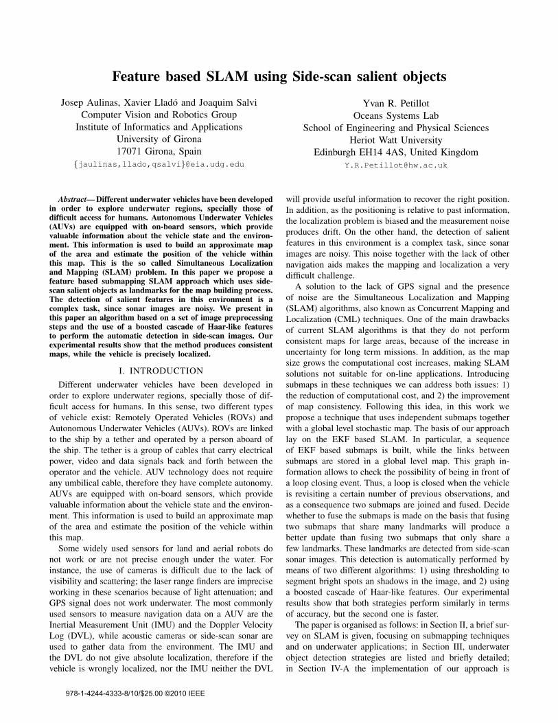
Abstract— Different underwater vehicles have been developedin order to explore underwater regions, specially those ofdifficult access for humans. Autonomous Underwater Vehicles(AUVs) are equipped with on-board sensors, which providevaluable information about the vehicle state and the environ-ment. This information is used to build an approximate mapof the area and estimate the position of the vehicle withinthis map. This is the so called Simultaneous Localizationand Mapping (SLAM) problem. In this paper we propose afeature based submapping SLAM approach which uses side-scan salient objects as landmarks for the map building process.The detection of salient features in this environment is acomplex task, since sonar images are noisy. We present inthis paper an algorithm based on a set of image preprocessingsteps and the use of a boosted cascade of Haar-like featuresto perform the automatic detection in side-scan images. Ourexperimental results show that the method produces consistentmaps, while the vehicle is precisely localized.
I. INTRODUCTION
Different underwater vehicles have been developed in
order to explore underwater regions, specially those of dif-
ficult access for humans. In this sense, two different types
of vehicle exist: Remotely Operated Vehicles (ROVs) and
Autonomous Underwater Vehicles (AUVs). ROVs are linked
to the ship by a tether and operated by a person aboard of
the ship. The tether is a group of cables that carry electrical
power, video and data signals back and forth between the
operator and the vehicle. AUV technology does not require
any umbilical cable, therefore they have complete autonomy.
AUVs are equipped with on-board sensors, which provide
valuable information about the vehicle state and the environ-
ment. This information is used to build an approximate map
of the area and estimate the position of the vehicle within
this map.
Some widely used sensors for land and aerial robots do
not work or are not precise enough under the water. For
instance, the use of cameras is difficult due to the lack of
visibility and scattering; the laser range finders are imprecise
working in these scenarios because of light attenuation; and
GPS signal does not work underwater. The most commonly
used sensors to measure navigation data on a AUV are the
Inertial Measurement Unit (IMU) and the Doppler Velocity
Log (DVL), while acoustic cameras or side-scan sonar are
used to gather data from the environment. The IMU and
the DVL do not give absolute localization, therefore if the
vehicle is wrongly localized, nor the IMU neither the DVL
will provide useful information to recover the right position.
In addition, as the positioning is relative to past information,
the localization problem is biased and the measurement noise
produces drift. On the other hand, the detection of salient
features in this environment is a complex task, since sonar
images are noisy. This noise together with the lack of other
navigation aids makes the mapping and localization a very
difficult challenge.
A solution to the lack of GPS signal and the presence
of noise are the Simultaneous Localization and Mapping
(SLAM) algorithms, also known as Concurrent Mapping and
Localization (CML) techniques. One of the main drawbacks
of current SLAM algorithms is that they do not perform
consistent maps for large areas, because of the increase in
uncertainty for long term missions. In addition, as the map
size grows the computational cost increases, making SLAM
solutions not suitable for on-line applications. Introducing
submaps in these techniques we can address both issues: 1)
the reduction of computational cost, and 2) the improvement
of map consistency. Following this idea, in this work we
propose a technique that uses independent submaps together
with a global level stochastic map. The basis of our approach
lay on the EKF based SLAM. In particular, a sequence
of EKF based submaps is built, while the links between
submaps are stored in a global level map. This graph in-
formation allows to check the possibility of being in front of
a loop closing event. Thus, a loop is closed when the vehicle
is revisiting a certain number of previous observations, and
as a consequence two submaps are joined and fused. Decide
whether to fuse the submaps is made on the basis that fusing
two submaps that share many landmarks will produce a
better update than fusing two submaps that only share a
few landmarks. These landmarks are detected from side-scan
sonar images. This detection is automatically performed by
means of two different algorithms: 1) using thresholding to
segment bright spots an shadows in the image, and 2) using
a boosted cascade of Haar-like features. Our experimental
results show that both strategies perform similarly in terms
of accuracy, but the second one is faster.
The paper is organised as follows: in Section II, a brief sur-
vey on SLAM is given, focusing on submapping techniques
and on underwater applications; in Section III, underwater
object detection strategies are listed and briefly detailed;
in Section IV-A the implementation of our approach is
978-1-4244-4333-8/10/$25.00 ©2010 IEEE
presented; in Section V the experiments and results are
provided; finally some conclusions are given in Section VI.
II. SIMULTANEOUS LOCALIZATION AND
MAPPING
SLAM is one of the fundamental challenges of
robotics [1]. The SLAM problem involves finding appropri-
ate representation for both the observation and the motion
models, which is generally performed by computing its prior
and posterior distributions using probabilistic algorithms, for
instance Kalman Filters (KF), Particle Filters (PF) and Ex-
pectation Maximization (EM). These probabilistic techniques
are very popular in the SLAM context because they tackle the
problem by modelling explicitly different sources of noise
and their effects on the measurements [2]. A well known
and widely used SLAM approach is the Extended Kalman
Filter SLAM (EKF-SLAM) [3]. EKF-SLAM represents the
vehicles pose and the location of a set of environment
features in a joint state vector. This vector is estimated and
updated by the EKF. EKF provides a suboptimal solution due
to several approximations and assumptions, which result in
divergences [4]. Several alternatives exist aiming to address
the linearisation approximations, for instance the Unscented
Kalman Filter [5], which uses a sigma points representation
to model noise distributions. In large areas, EKF complexity
grows with the number of landmarks, because each landmark
is correlated to all other landmarks. This means that EKF
memory complexity is O(n2) and a time complexity of
O(n2) per step, where n is the total number of features
stored in the map. Different approaches aiming to reduce
this computational cost have been presented, for instance, the
Compressed Extended Kalman Filter [6] delays the update
stage after several observations; while the Exactly sparse
extended information filters [7] take advantage of the sparsity
in the information matrix, reducing considerably the com-
putational demand. The two following sections summarize
the state-of-the-art SLAM approaches in A) submapping
techniques, and B) underwater applications.
A. Submapping techniques
Using submaps addresses both issues, reduces computa-
tional cost and improves map consistency. An example of
submapping approach is the Decoupled Stochastic Map [8],
which uses non-statistically independent submaps, therefore
the correlations are broken introducing inconsistency in
the map. Something similar happens in [9], where local
maps share information while kept independent, thus a
long term mission diverges. Different techniques, such as
the Constrained Local Submap Filter [10] or Local Map
Joining [11] produce efficient global maps by consistently
combining completely independent local maps. The Divide
and Conquer [12] approach is able to recover the global map
in approximately O(n) time. The Conditionally Independent
Local Maps [13] method is based on sharing information
between consecutive submaps. This way, a new local map is
initialised considering the a-priori knowledge. The Constant
Time SLAM [14], the Atlas approach [15] and the Hierar-
chical SLAM [16] store the link between submaps by means
of an adjacency graph. The later imposes loop constraints on
the adjacency graph, producing a better estimate of the global
level map. Finally, in [17] a Selective Submap Joining SLAM
was proposed, this approach is detailed in further sections as
it is the one used in our implementation.
B. Underwater approaches
Multiple techniques have shown promising results in a
variety of different applications and scenarios. Some of them
perform SLAM indoors where the scenario is structured and
simpler as compared to outdoor environments. Underwater
scenarios are still one of the most challenging scenarios for
SLAM because of the reduced sensorial possibilities and the
difficulty in finding reliable features. A SLAM solution for
underwater environments tackles the problem using feature
based techniques [18]. However, such approaches have many
problems due to the unstructured nature of the seabed and
the difficulty to identify reliable features. Many underwater
features are scale dependant, sensitive to viewing angle and
small. On the other hand, a non-feature based approach to
SLAM that utilizes a 2D grid structure to represent the
map and a Distributed Particle Filter to track the uncertainty
in the vehicle state was presented in [19]. They named
their method as the Bathymetric distributed Particle SLAM
(BPSLAM) filter. BPSLAM does not need to explicitly
identify features in the surrounding environment or apply
complicated matching algorithms. On the other hand, they
required a prior low-resolution map generated by a surface
vessel.
Another approach utilizes a 3D occupancy grid map
representation, efficiently managed with Deferred Reference
Counting Octrees [20]. A particle filter is used to handle
the uncertainty in the navigation solution provided by the
vehicle. This approach was successful in minimizing the
navigation error during a deep sea mapping mission. How-
ever, map based localization was only available after the map
building process had been carried out. This prohibited any
corrections in navigation during the map building process.
A vision-based localization approach for an underwater
robot in a structured environment was presented in [21].
Their system was based on a coded pattern placed on the
bottom of a water tank and an on-board down-looking
camera. The system provided three-dimensional position and
orientation of the vehicle along with its velocity. Another
vision-based algorithm [22] used inertial sensors together
with the typical low-overlap imagery constraints of under-
water imagery. Their strategy consisted on solving a sparse
system of linear equations in order to maintain consistent
covariance bound within a SLAM information filter. The
main limitation on vision-based techniques is that they are
limited to near field vision (1-5m), and also deep water
mission will require higher amounts of energy for lighting
purposes.
Instead of vision, in [23] a mechanically scanned imaging
sonar is used to obtained information about the location of
vertical planar structures present in partially structured envi-
ronments. In this approach, the authors extract line features
from sonar data, by means of a robust voting algorithm.
These line features are used into a Kalman filter base SLAM.
In [24] a side-scan sonar was used to sense the environment.
The returns from the sonar were used to detect landmarks
in the vehicles vicinity. Reobserving these landmarks allows
to correct the map and vehicle location, however after
long distances the drift is too large to allow associating
landmarks with current observations. For this reason, they
proposed a method that combines a forward stochastic map
in conjunction with a backward Rauch-Tung-Striebel filter
to smooth the trajectory. Another approach using side-scan
sonar is presented in [25]. In that paper, the whole scenario
is built through EKF based submaps, producing a consistent
map and localizing the vehicle efficiently. The same strategy
is used in this paper together with the automatic detection
of salient features from side-scan sonar images. As side
scan sonars provide higher quality images than forward-look
sonars, the object detection and the data association becomes
easier.
III. OBJECT DETECTION AND MATCHING
A great number of papers discussing image segmentation,
classification, registration, and landmark extraction have al-
ready been published. Thresholding and clustering theory
has been used in [26] to segment the side-scan sonar image
into regions of object-highlight, shadow, and background.
Similarly, the system in [27] utilizes an adaptive thresholding
technique to detect and extract geometric features for both
the shadow and the object. Another unsupervised model for
both the detection and the shadow extraction as an automated
classification system was presented in [28]. Using spatial
information on the physical size and geometric signature
of mines in side-scan sonar, a Markov random field (MRF)
model segments the image into regions. A cooperating statis-
tical snake (CSS) model is used to extract the highlight and
shadow of the object. Features are extracted so that the object
can be classified. A more recent approach [29], first extracts
texture features from side scan images. A region based active
contour model is then applied to segment significant objects.
The Viola-Jones object detection framework is capable to
provide competitive object detection rates [30]. It can be
trained to detect a variety of object classes. In this paper, we
implemented two different methods to detect objects from
side-scan sonar images, one based on thresholding and the
other one based on Viola-Jones (further details are given in
Section IV-B).
IV. IMPLEMENTATION
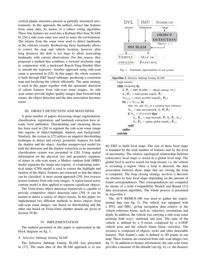
The method presented in this paper is represented in the
block diagram on fig. 1.
A. Selective Submap Joining SLAM
The Selective Submap Joining SLAM was presented
in [17]. The main idea of this SLAM approach is to use
Fig. 1. Schematic representation of our system
Algorithm I: Selective Submap Joining SLAM
begin mission
while navigating do
xi, Pi = EKF SLAM() ← (Build submap Mi)
xG, PG = build global map(xi, Pi)
HLoop = check possible loops(xG, PG)
for j = HLoop do
refer Mi and Mj to a common base reference
Hij = data association(xi, xj , Pi, Pj )
if Hij > threshold then
xij , Pij = map fusion(xi, Pi, xj , Pj , Hij )
xG, PG = update global map(xij , Pij )
endif
endfor
endwhile
the EKF to build local maps. The size of these local maps
is bounded by the total number of features and by the level
of uncertainty. The relative topological relationship between
consecutive local maps is stored in a global level map. The
global level is used to search for loop closure, i.e. the vehicle
is revisiting a region. Once a loop is detected, the data
association between those maps that are closing the loop
is computed. The loop closing strategy involves a decision
on whether to fuse local maps depending on the amount of
found correspondences. This correspondences are computed
by means of a Joint Compatibility Branch and Bound [31]
data association algorithm. The whole process is presented
in Algorithm I.
The AUV REMUS-100 was used to gather the experi-
mental data (see fig. 2). The vehicle was equipped with
a DVL and IMU, giving navigation data relative to the
vehicle reference frame, such as, velocities, orientations and
depth. In addition, the vehicle was carrying a side-scan sonar
pointing both ways, starboard and port. The state of the
vehicle is defined by a 9-vector, composed by a 6-DOF
vehicle pose and the vehicle frame linear velocities. The
scenario is composed of objects, rocks and other detectable
features. This feature’s state is defined as 3D points in our
map. These features are extracted from side-scan images (see
fig. 3). In addition to feature information, the side-scan sonar
provides a measure of the altitude (see fig. 4), i.e. the distance
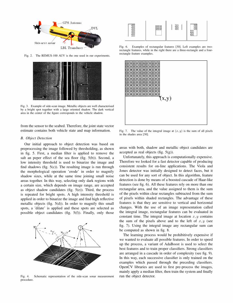
Fig. 2. The REMUS-100 AUV is the one used in our experiments.
Fig. 3. Example of side-scan image. Metallic objects are well characterisedby a bright spot together with a large oriented shadow. The dark verticalarea in the center of the figure corresponds to the vehicle shadow.
from the sensor to the seabed. Therefore, the joint state vector
estimate contains both vehicle state and map information.
B. Object Detection
Our initial approach to object detection was based on
preprocessing the image followed by thresholding, as shown
in fig. 5. First, a median filter is applied to remove the
salt an peper effect of the sea floor (fig. 5(b)). Second, a
low intensity threshold is used to binarize the image and
find shadows (fig. 5(c)). The resulting image is run through
the morphological operation ’erode’ in order to magnify
shadow sizes, while at the same time joining small noise
areas together. In this way, selecting only dark regions with
a certain size, which depends on image range, are accepted
as object shadow candidates (fig. 5(e)). Third, the process
is repeated for bright spots. A high intensity threshold is
applied in order to binarize the image and find high reflective
metallic objects (fig. 5(d)). In order to magnify this small
spots, a ’dilate’ is applied and these spots are selected as
possible object candidates (fig. 5(f)). Finally, only those
Fig. 4. Schematic representation of the side-scan sonar measurementprocedure.
Fig. 6. Examples of rectangular features [30]. Left examples are two-rectangle features, while in the right there are a three-rectangle and a four-rectangle feature examples.
Fig. 7. The value of the integral image at (x, y) is the sum of all pixelsin the shades area [30].
areas with both, shadow and metallic object candidates are
accepted as real objects (fig. 5(g)).
Unfortunately, this approach is computationally expensive.
Therefore we looked for a fast detector capable of producing
consistent results for on-line applications. The Viola and
Jones detector was initially designed to detect faces, but it
can be used for any sort of object. In this algorithm, feature
detection is done by means of a boosted cascade of Haar-like
features (see fig. 6). All these features rely on more than one
rectangular area, and the value assigned to them is the sum
of the pixels within clear rectangles subtracted from the sum
of pixels within shaded rectangles. The advantage of these
features is that they are sensitive to vertical and horizontal
changes. With the use of an image representation called
the integral image, rectangular features can be evaluated in
constant time. The integral image at location x, y contains
the sum of the pixels above and to the left of x, y (see
fig. 7). Using the integral image any rectangular sum can
be computed as shown in fig. 8.
The learning process would be prohibitively expensive if
we wanted to evaluate all possible features. In order to speed
up the process, a variant of AdaBoost is used to select the
best features and to train proper classifiers. Strong classifiers
are arranged in a cascade in order of complexity (see fig. 9).
In this way, each successive classifier is only trained on the
examples which passed through the preceding classifiers.
OpenCV libraries are used to first pre-process the images,
mainly apply a median filter, then train the system and finally
run the object detector.
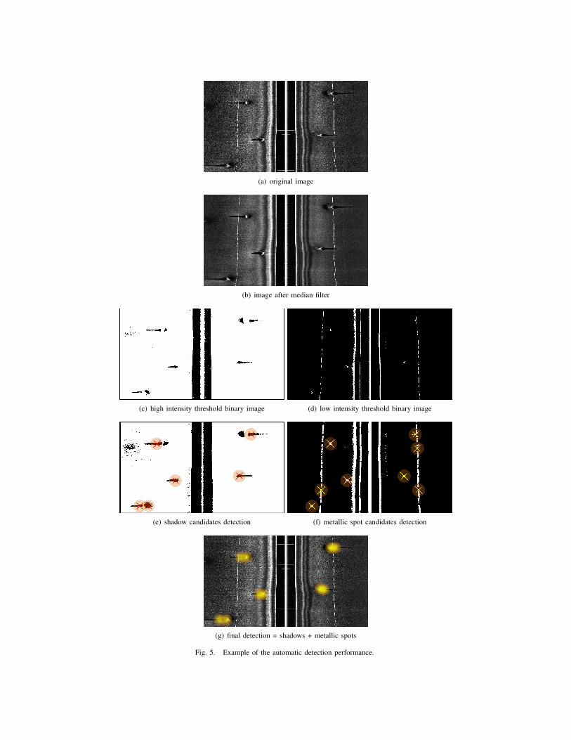
(a) original image
(b) image after median filter
(c) high intensity threshold binary image (d) low intensity threshold binary image
(e) shadow candidates detection (f) metallic spot candidates detection
(g) final detection = shadows + metallic spots
Fig. 5. Example of the automatic detection performance.
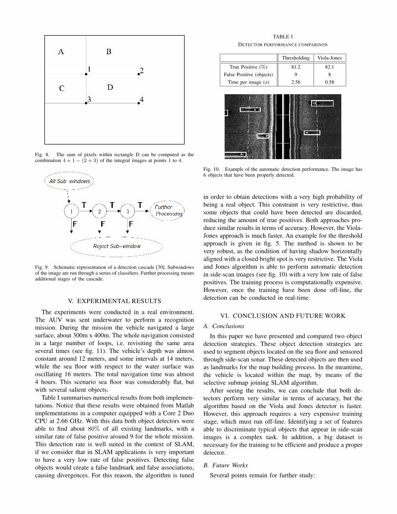
Fig. 8. The sum of pixels within rectangle D can be computed as thecombination 4 + 1− (2 + 3) of the integral images at points 1 to 4.
Fig. 9. Schematic representation of a detection cascade [30]. Subwindowsof the image are run through a series of classifiers. Further processing meansadditional stages of the cascade.
V. EXPERIMENTAL RESULTS
The experiments were conducted in a real environment.
The AUV was sent underwater to perform a recognition
mission. During the mission the vehicle navigated a large
surface, about 300m x 400m. The whole navigation consisted
in a large number of loops, i.e. revisiting the same area
several times (see fig. 11). The vehicle’s depth was almost
constant around 12 meters, and some intervals at 14 meters,
while the sea floor with respect to the water surface was
oscillating 16 meters. The total navigation time was almost
4 hours. This scenario sea floor was considerably flat, but
with several salient objects.
Table I summarises numerical results from both implemen-
tations. Notice that these results were obtained from Matlab
implementations in a computer equipped with a Core 2 Duo
CPU at 2.66 GHz. With this data both object detectors were
able to find about 80% of all existing landmarks, with a
similar rate of false positive around 9 for the whole mission.
This detection rate is well suited in the context of SLAM,
if we consider that in SLAM applications is very important
to have a very low rate of false positives. Detecting false
objects would create a false landmark and false associations,
causing divergences. For this reason, the algorithm is tuned
TABLE I
DETECTOR PERFORMANCE COMPARISON
Thresholding Viola-Jones
True Positive (%) 81.2 82.1
False Positive (objects) 9 8
Time per image (s) 2.56 0.58
Fig. 10. Example of the automatic detection performance. The image has6 objects that have been properly detected.
in order to obtain detections with a very high probability of
being a real object. This constraint is very restrictive, thus
some objects that could have been detected are discarded,
reducing the amount of true positives. Both approaches pro-
duce similar results in terms of accuracy. However, the Viola-
Jones approach is much faster. An example for the threshold
approach is given in fig. 5. The method is shown to be
very robust, as the condition of having shadow horizontally
aligned with a closed bright spot is very restrictive. The Viola
and Jones algorithm is able to perform automatic detection
in side-scan images (see fig. 10) with a very low rate of false
positives. The training process is computationally expensive.
However, once the training have been done off-line, the
detection can be conducted in real-time.
VI. CONCLUSION AND FUTURE WORK
A. Conclusions
In this paper we have presented and compared two object
detection strategies. These object detection strategies are
used to segment objects located on the sea floor and sensored
through side-scan sonar. These detected objects are then used
as landmarks for the map building process. In the meantime,
the vehicle is located within the map, by means of the
selective submap joining SLAM algorithm.
After seeing the results, we can conclude that both de-
tectors perform very similar in terms of accuracy, but the
algorithm based on the Viola and Jones detector is faster.
However, this approach requires a very expensive training
stage, which must run off-line. Identifying a set of features
able to discriminate typical objects that appear in side-scan
images is a complex task. In addition, a big dataset is
necessary for the training to be efficient and produce a proper
detector.
B. Future Works
Several points remain for further study:
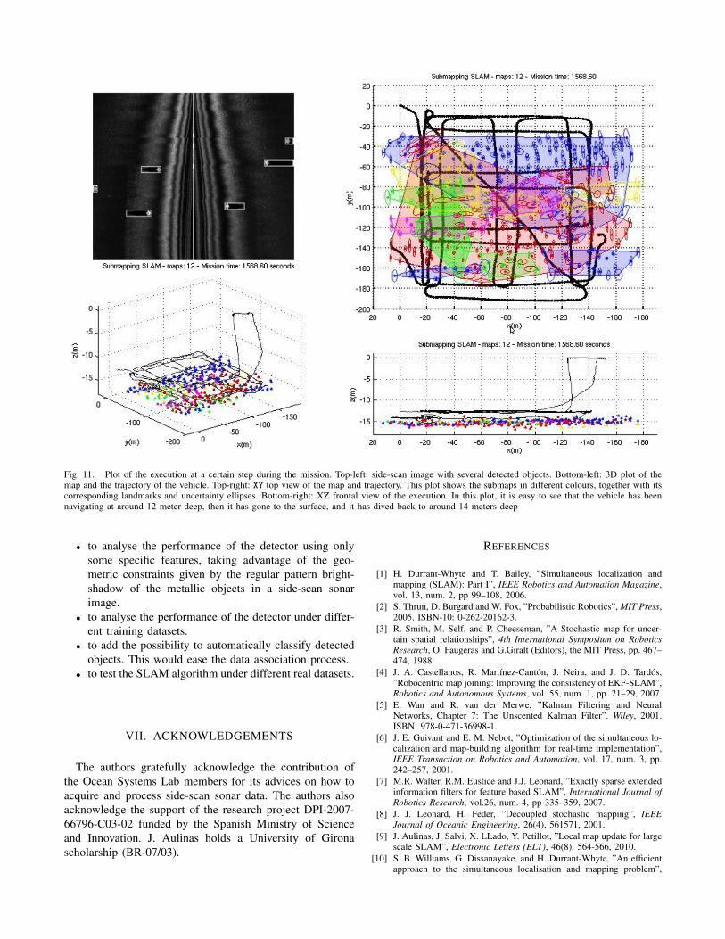
Fig. 11. Plot of the execution at a certain step during the mission. Top-left: side-scan image with several detected objects. Bottom-left: 3D plot of themap and the trajectory of the vehicle. Top-right: XY top view of the map and trajectory. This plot shows the submaps in different colours, together with itscorresponding landmarks and uncertainty ellipses. Bottom-right: XZ frontal view of the execution. In this plot, it is easy to see that the vehicle has beennavigating at around 12 meter deep, then it has gone to the surface, and it has dived back to around 14 meters deep
• to analyse the performance of the detector using only
some specific features, taking advantage of the geo-
metric constraints given by the regular pattern bright-
shadow of the metallic objects in a side-scan sonar
image.
• to analyse the performance of the detector under differ-
ent training datasets.
• to add the possibility to automatically classify detected
objects. This would ease the data association process.
• to test the SLAM algorithm under different real datasets.
VII. ACKNOWLEDGEMENTS
The authors gratefully acknowledge the contribution of
the Ocean Systems Lab members for its advices on how to
acquire and process side-scan sonar data. The authors also
acknowledge the support of the research project DPI-2007-
66796-C03-02 funded by the Spanish Ministry of Science
and Innovation. J. Aulinas holds a University of Girona
scholarship (BR-07/03).
REFERENCES
[1] H. Durrant-Whyte and T. Bailey, ”Simultaneous localization andmapping (SLAM): Part I”, IEEE Robotics and Automation Magazine,vol. 13, num. 2, pp 99–108, 2006.
[2] S. Thrun, D. Burgard and W. Fox, ”Probabilistic Robotics”, MIT Press,2005. ISBN-10: 0-262-20162-3.
[3] R. Smith, M. Self, and P. Cheeseman, ”A Stochastic map for uncer-tain spatial relationships”, 4th International Symposium on Robotics
Research, O. Faugeras and G.Giralt (Editors), the MIT Press, pp. 467–474, 1988.
[4] J. A. Castellanos, R. Martınez-Canton, J. Neira, and J. D. Tardos,”Robocentric map joining: Improving the consistency of EKF-SLAM”,Robotics and Autonomous Systems, vol. 55, num. 1, pp. 21–29, 2007.
[5] E. Wan and R. van der Merwe, ”Kalman Filtering and NeuralNetworks, Chapter 7: The Unscented Kalman Filter”. Wiley, 2001.ISBN: 978-0-471-36998-1.
[6] J. E. Guivant and E. M. Nebot, ”Optimization of the simultaneous lo-calization and map-building algorithm for real-time implementation”,IEEE Transaction on Robotics and Automation, vol. 17, num. 3, pp.242–257, 2001.
[7] M.R. Walter, R.M. Eustice and J.J. Leonard, ”Exactly sparse extendedinformation filters for feature based SLAM”, International Journal of
Robotics Research, vol.26, num. 4, pp 335–359, 2007.
[8] J. J. Leonard, H. Feder, ”Decoupled stochastic mapping”, IEEE
Journal of Oceanic Engineering, 26(4), 561571, 2001.
[9] J. Aulinas, J. Salvi, X. LLado, Y. Petillot, ”Local map update for largescale SLAM”, Electronic Letters (ELT), 46(8), 564-566, 2010.
[10] S. B. Williams, G. Dissanayake, and H. Durrant-Whyte, ”An efficientapproach to the simultaneous localisation and mapping problem”,
IEEE Int. Conf. on Robotics and Automation, vol. 1, pp. 406–411,2002.
[11] J. D. Tardos, J. Neira, P. M. Newman, and J. J. Leonard, ”Robustmapping and localization in indoor environments using sonar data”,International Journal on Robotics Research, vol. 21, num. 4, pp. 311–330, 2002.
[12] L. M. Paz, J. D. Tardos, and J. Neira, ”Divide and conquer: EKFSLAM in O(n)”, IEEE Transaction in Robotics, vol. 24, num. 5, pp.1107–1120, 2008.
[13] P. Pinies and J. D. Tardos, ”Large Scale SLAM Building ConditionallyIndependent Local Maps: Application to Monocular Vision”, IEEE
Transactions on Robotics, vol. 24, no. 5, October 2008.[14] P.M. Newman and J.J. Leonard, ”Consistent, convergent, and constant-
time SLAM”, Int. Joint Conf. on Artificial Intelligence (IJCAI), pp.1143–1150, 2003.
[15] M. Bosse, P. M. Newman, J. J. Leonard, and S. Teller, ”SLAM in largescale cyclic environments using the atlas framework”, Int. Journal in
Robotics Research, vol. 23, num. 12, pp. 1113–1139, 2004.[16] C. Estrada, J. Neira, and J. D. Tardos, ”Hierarchical SLAM: real-
time accurate mapping of large environments”, IEEE Transaction in
Robotics, vol. 21, num. 4, pp. 588–596, 2005.[17] J. Aulinas, X. LLado, J. Salvi, Y. Petillot, ”SLAM base Selective
Submap Joining for the Victoria Park Dataset”, 7th IFAC Symposium
on Intelligent Autonomous Vehicles (IFAC/IAV), Lecce (Italy) Septem-ber 6-8, 2010.
[18] S.B. Williams, ”Efficient Solutions to Autonomous Mapping and Nav-igation Problems”, PhD thesis, Australian Centre for Field Robotics -The University of Sydney, 2001.
[19] S. Barkby, S.B. Williams, O. Pizarro, M. Jakuba, ”Incorporating priorbathymetric maps with distributed particle bathymetric SLAM forimproved AUV navigation and mapping”, in Proceedings MTS/IEEE
Oceans Conference and Exhibition, Biloxi (USA), 2009.[20] N. Fairfield, D. Wettergreen. Active localization on the ocean floor
with multibeam sonar, In Proceedings of MTS/IEEE OCEANS, 2008.[21] M. Carreras, P. Ridao, R. Garcia, and T. Nicosevici, ”Vision-based
localization of an underwater robot in a structured environment”, IEEE
International Conference on Robotics and Automation, 2003. ICRA03, vol. 1, pp. 971–976, 2003.
[22] R. Eustice, O. Pizarro, and H. Singh, ”Visually Augmented Navigationfor Autonomous Underwater Vehicles”, IEEE Journal of Oceanic
Engineering, 33(2):103 – 122, April. 2008.[23] D. Ribas, P. Ridao, J.D. Tards and J. Neira, ”Underwater SLAM
in Man Made Structured Environments”, Journal of Field Robotics,25(11-12):898–921, 2008.
[24] I. Tena-Ruiz, S. Raucourt, Y. Petillot, and D. Lane, Concurrentmapping and localization using side-scan sonar, IEEE Journal of
Oceanic Engineering, vol. 29, no. 2, pp. 442–456, 2004.[25] J. Aulinas, C.S. Lee, J. Salvi, Y. Petillot, ”Submapping SLAM
based on acoustic data from a 6-DOF AUV”, 8th IFAC Conference
on Control Applications in Marine Systems (IFAC/CAMS), Rostock-Warnemnde (Germany), September 15-17, 2010.
[26] S. G. Johnson and M. A. Deaett, The application of automatedrecognition techniques to side-scan sonar imagery, IEEE Journal of
Oceanic Engineering, vol. 19, pp. 138–144, 1994.[27] C. M. Ciany and J. Huang, Computer aided detection/computer aided
classification and data fusion algorithms for automated detectionand classification of underwater mine, in Proc. MTS/IEEE Oceans
Conference and Exhibition, vol. 1, pp. 277–284, 2000.[28] S. Reed, Y.R. Petillot, J. Bell, ”An Automatic Approach to the
Detection and Extraction of Mine Features in Side-scan Sonar”, IEEE
Journal of Oceanic Engineering, vol. 28, no. 1, pp. 90–105, 2003.[29] M. Lianantonakis, Y. petillot, ”Side-scan Sonar Segmentation Using
Texture Descriptors and Active Contours”, IEEE Journal of Oceanic
Engineering, vol. 32, pp. 744–752, 2007.[30] P.A. Viola, M. J. Jones, ”Rapid Object Detection using a Boosted
Cascade of Simple Features”, IEEE Conference on Computer Vision
and Pattern Recognition (CVPR), vol. 1, pp. 511–518, 2001.[31] J. Neira and J.D. Tardos, ”Data Association in Stochastic Mapping
Using the Joint Compatibility Test”, IEEE Transaction on Robotics
and Automation, vol. 17, num. 6, pp. 890–897, Dec 2001.
Recommended