1
Exploiting a Geometrically Sampled Grid in theSRP-PHAT for Localization Improvement and
Power Response Sensitivity AnalysisDaniele Salvati, Carlo Drioli, and Gian Luca Foresti,
Abstract—The steered response power phase transform (SRP-PHAT) is a beamformer method very attractive in acoustic local-ization applications due to its robustness in reverberant environ-ments. This paper presents a spatial grid design procedure, calledthe geometrically sampled grid (GSG), which aims at computingthe spatial grid by taking into account the discrete samplingof time difference of arrival (TDOA) functions and the desiredspatial resolution. A new SRP-PHAT localization algorithm basedon the GSG method is also introduced. The proposed methodexploits the intersections of the discrete hyperboloids representingthe TDOA information domain of the sensor array, and projectsthe whole TDOA information on the space search grid. The GSGmethod thus allows to design the sampled spatial grid whichrepresents the best search grid for a given sensor array, it allowsto perform a sensitivity analysis of the array and to characterizeits spatial localization accuracy, and it may assist the systemdesigner in the reconfiguration of the array. Experimental resultsusing both simulated data and real recordings show that thelocalization accuracy is substantially improved both for high andfor low spatial resolution, and that it is closely related to theproposed power response sensitivity measure.
Index Terms—Sound source localization, steered responsepower, acoustic beamforming, SRP-PHAT, geometrically sampledgrid, power response sensitivity analysis, microphone array,reverberant environment.
I. INTRODUCTION
THE problem of locating acoustic sources is a funda-mental task in applications of acoustic scene analysis
and acoustic situational awareness, and it received significantattention in the research community. Direct methods based onthe processing and fusion of data collected from microphonearrays are very attractive in acoustic applications due to theirrobustness and fast implementation [1]–[6].
The steered response power phase transform (SRP-PHAT)[2] is one of the most effective direct methods for the local-ization of acoustic sources in reverberant environments. It isbased on a steered beamformer, which can be implementedusing a space search procedure, and a map that links eachposition of the search grid to the time difference of arrival(TDOA) functions related to the sensor pairs. The sourceposition is then estimated by maximization of a specificfunction that provides a coherent value from the entire systemof microphones. The localization function is the sum of thegeneralized cross-correlation phase transform (GCC-PHAT)
D. Salvati, C. Drioli, and G.L. Foresti are with the Department of Mathe-matics and Computer Science, University of Udine, Udine 33100, Italy, e-mail:[email protected], [email protected], [email protected].
[7] values estimated from all combinations of microphonepairs.
The use of an acoustic map related to the TDOA be-tween two microphones has been first introduced in 1998 byOmologo and De Mori [1]. The authors call this procedureglobal coherence field (GCF), and introduce the GCF-PHAT[8] method, which is equivalent to SRP-PHAT. In 2001,the authors of [2] demonstrated that the SRP-PHAT can becomputed by decomposing the steered beamformer into thesum of the beamformers corresponding to the sensor pairsof the array, and that the steered response of two sensors isequivalent to the GCC-PHAT function. Thus, the SRP-PHATis effectively computed by using the GCF and the GCC-PHAT,making its practical implementation very attractive. In fact, theGCC-PHAT can be computed in the frequency domain usingthe fast Fourier transform (FFT) for each sensor pair, and theacoustic map can be computed by access and sum operationson a look-up table of GCC-PHAT values. The sampled spacegrid, which is a set of candidate positions for the source, ispre-calculated defining a look-up table that links the positionin space with TDOA values of microphone pairs.
Note that the SRP-PHAT algorithm is actually the com-bination of two distinct components: the steered responsepower (SRP) computation and a PHAT prefiltering. The roleof the PHAT filter is to normalize the narrowband steeredbeamformer and to only take into account the phases ofthe cross-power spectral density. The normalization has thepositive effect of increasing the spatial resolution [9], andit is one of the advantage of this method in a reverberantenvironment since it allows improved identification of directpaths and reflections.
Most part of the past researches on SRP-PHAT focusedon solutions to reduce the computational cost of the grid-search step. In some cases, the problem has been faced bycalculating the steered response on a limited set of candidatesource positions, e.g, by using a stochastic region contraction[10], by using a generic doubly hierarchical search algorithm[11], or by only considering the larger GCC-PHAT coefficients[12]. However, these methods usually discard part of theinformation available and the localization performance candegrade when reverberation increases [13]. In [12], since theGCC-PHAT function provides different local maxima due tothe contribution of direct-path and early reflections, when thedirect-path peak has lower intensity with respect to a reflectionpeak, the peak picking procedure returns a wrong contributionsince it disregards the direct-path peak in favor of a reflection
arX
iv:1
512.
0326
1v4
[cs
.SD
] 7
Mar
201
8
2
peak.Recently, a method that relies on the use of a coarser
grid has been proposed in [14]. Herein it is shown that thetraditional grid-search approach of SRP-PHAT degrades itsperformance when the spatial resolution decreases due to theloss of information of GCC-PHAT functions. To face thisproblem, in [14] a scalable spatial sampling (SSS) is proposedto accumulate the GCC-PHAT values in a range that coversthe volume surrounding each point of the defined spatialgrid. The GCC-PHAT accumulation limits are determinedby the gradient of the inter-microphone time delay functioncorresponding to each microphone pair. The reduced numberof spatial grid points involves a lower computational cost, butthe accuracy is limited by the resolution of the grid. Othermethods have been proposed that improve the localizationaccuracy by refining the search procedure from a coarser gridto a finer grid using iterative searching procedures [13], [15],[16].
The above mentioned methods have in common the way inwhich the space search grid is designed, and the way in whichthe relationship between the points on the grid and the TDOAsof microphone pairs is build. Specifically, for each microphonepair and for each point on the grid, an unique integer TDOAvalue is selected to be the acoustic delay information linkedto that point. This uniform regular grid (URG) procedure doesnot guarantee that all TDOA samples are associated to pointson the grid, nor that the spatial grid is consistent since some ofthe points in the grid may not correspond to an intersection ofa bare minimum of three hyperboloids (or two hyperbolas, in2D). The linking from space points on the grid to TDOAsalso does not allow for spatial resolution scalability, sincewhen the number of points is reduced, part of the TDOAinformation gets lost as it results no more associated to anypoints on the grid. For these reasons, different methods havebeen proposed in [13]–[15] to collect and use the TDOAinformation related to the volume surrounding each spatialpoint on the search grid. A boundary-vertex (BV) approachis used in [13], in which the GCC-PHAT accumulation limitsare determined by the cube surrounding the volume vertices. In[15], a modified SSS (MSSS) is proposed , which exploits themean of the accumulated GGC-PHAT values for each volume.However, these methods does not take into account how TDOAinformation is distributed in the space. We will see that thespatial distribution of all TDOA information is an importantinformation that can be used to compute a sensitivity measureof the acoustic system with respect to the search region and toimprove the localization accuracy. There is thus the need of arigorous analysis of the spatial grid map and of how the TDOAinformation from GCC-PHAT functions is accumulated in thespace.
In this paper, we study the properties of the SRP-PHATalgorithm focusing especially on the grid resolution, whichis in general arbitrarily imposed depending on the type ofapplication, and the TDOA resolution, which is given by thedistance between the microphones and the sample rate usedin the digital system. We propose a new spatial grid designprocedure, named geometrically sampled grid (GSG), whichmakes use of the discrete hyperboloids (representing all pos-
sible locations related to a TDOA) and of their intersections,to design an acoustically-coherent space grid on which thesource search can be performed.
Moreover, we will show how, based on the density analysisof hyperboloid intersections, a steered power response sensi-tivity analysis of the localization system can be conducted.We refer herein to sensitivity as a quantified measure of thechange of the response power with respect to the change ofthe spatial position, predicting where the search space will becharacterized by higher and lower localization accuracy. Todate, studies concerning the information distribution of SRP-like localization methods are not frequent in the literature.An example is [17], in which a discriminability measure isproposed, which only considers the array geometry and thesampling frequency to distinguish a given point in space fromits neighbors. In contrast with it, the proposed GSG includesin the analysis process a relationship between the sampledspace and all discrete samples of the GCC-PHAT functions toprevent the loss of information that may arise from the choiceof an arbitrary desired spatial resolution.
Besides that, the coherent sample grid and the powerresponse sensitivity analysis are useful tools to decide if thespatial resolution and the sensitivity map of a given arrayconfiguration are adequate and, if not, to assist the systemdesigner in its reconfiguration (e.g., by the positioning ofadditional sensors or by increasing the sampling frequency).Hence, it means that the system configuration designed bythe GSG procedure generates a grid in which each point isconsistent for the localization, i.e. it is the point of intersectionof at least three hyperboloids.
With respect to other approaches whose aim is to improvethe localization accuracy, the GSG method builds the steeredpower response function using all the TDOA informationavailable from the GCC-PHAT functions related to the sensorpairs in the array, it solves the problem of arbitrarily selectingthe spatial grid resolution without loss of information, and itturns out to notably improve the localization performances.The geometric approach based on the analysis of hyperboloidintersections allows the design of a sensitivity map, in whichthe regions where the localization is more accurate correspondto the high sensitivity regions of the steered power responsefunction.
Finally, the GSG method might also provides reduced com-putational cost with respect to the URG method in three cases:1. when the search procedure is restricted to the coherent grid,thus discarding the URG points which are not covered bysufficient acoustic information, 2. when the type of applicationallows to use a coarser grid and a lower spatial resolution, 3.when the search can be restricted only to the high sensitivityregions, in which the localization accuracy is maximized.
The paper is organized as follows. After presenting therelationship between the spatial grid and the TDOA functionsin Section II, the SRP-PHAT method is described in SectionIII. In Section IV the GSG algorithm and the GSG based SRP-PHAT are presented. Finally, Section V illustrates experimen-tal results obtained in a simulated reverberant environment andin a real-world scenario.
3
II. SPATIAL GRID AND TIME DIFFERENCE OF ARRIVAL
Consider a reverberant room, and a location volume G =(Gx × Gy × Gz), discretized with a space resolution ∆, inwhich the acoustic source is searched. A generic grid positionis denoted by rg = [xg yg zg]
T , rg ∈ G. Within the room,we suppose M microphones disposed according to a givengeometry. The positions of the M microphones in Cartesiancoordinates are
rm = [xm ym zm]T , m = 1, 2, . . . ,M (1)
where (·)T denotes the transpose operator. We will consider allpossible sensor pairs of the array in our analysis. Accordingly,an array of M microphones provides N unique microphonepairs, with
N =
(M
2
). (2)
Given a generic sensor pair n, referred to two microphoneslocated in ri and rj , the maximum TDOA in samples Tn ∈ Zis obtained as
Tn = fix( ||ri − rj ||fs
c
)(3)
where fix(·) denotes the round toward zero operation, fs isthe sampling frequency, c is the speed of sound, and || · ||denotes Euclidean norm. The admissible range of values forthe TDOA is [-Tn,Tn], thus the possible TDOA values for thesensor pair n are 2Tn + 1.
We study the case in which a single acoustic source is activeat time k and the unknown coordinate position is
rs(k) = [xs(k) ys(k) zs(k)]T . (4)
The observed signals are given by the convolution of theunknown source s(k) with corresponding acoustic impulseresponses hm from the source to the microphone m. Thereverberant model for discrete-time signals can be expressedas
xm(k) = hm ∗ s(k) + vm(k) (5)
where m = 1, 2, . . . ,M , ∗ denotes convolution, vm(k) is theuncorrelated noise signal. The relationship between a genericspace position rg and the TDOA of the wavefront at the sensorpair n of two microphones i and j becomes
τn(rg) = round[ (||rg − ri|| − ||rg − rj ||)fs
c
](6)
where round[·] denotes rounding operator. Note that equation(6) assumes that the TDOA is an integer and it is expressedin samples. Equation (6) represents an hyperboloid, whichdescribes the locus of possible sound source locations gen-erating the same TDOA for that microphone pair. To uniquelydetermine the position of the source (the three unknowncoordinates), we need, at a bare minimum, a system of threeequations providing the intersection of the three hyperboloids.
The spatial grid in the SRP-PHAT algorithm is traditionallycalculated with an URG approach that links the uniformlydistributed points on the spatial grid to TDOAs related to thesensor pairs.
Given a look-up table χ(rg, n) which stores the relationshipbetween grid positions and TDOAs, the URG procedure is
Algorithm 1 URG AlgorithmN : number of microphone pairsfor all rg ∈ G do
for n = 1 to N doCalculate τn(rg) by means of Eq. (6)χ(rg, n) = τn(rg)
end forend for
summarized in Algorithm 1. The limitations of this approachare that it does not guarantee that all TDOA values correspondto a point on the space grid (and if this is the case, theinformation related to that TDOA is lost), and that it is notguaranteed that every point of the grid is consistent with thecondition of being the locus where at least three hyperboloidsintersect. Note that, due to the rounding operator, from theURG point of view everything goes as if in each grid positionthere is an intersection of N hyperboloids. The approximationdue to the rounding operation can link a whole set of neighborpoints to the same TDOA, resulting in practice in an uniformsteered response power in that region.
III. STEERED RESPONSE POWER PHASE TRANSFORM
The steered beamformer for source localization is basedon the computation of a filtered combination of the delayedsignals sensed by the array. Typically, a broadband steeredpower beamformer is computed in the frequency-domain byapplying a FFT on a portion of the signal and by calculatingthe response power on each frequency bin. Subsequently, afusion of these estimates is computed. The narrowband outputsignal of a delay and sum beamforming can be expressed as
Y (f, rg, k) = AH(f, rg)X(f, k) (7)
where f is the frequency index, the superscript H representsthe Hermitian (complex conjugate) transpose, A(f, rg) isthe steering vector corresponding to a given position rg ,X(f, k) = [X1(f, k)X2(f, k) . . . XM (f, k)]T , Y (f, rg, k) andXm(f, k), m = 1, 2, . . . ,M , are the FFT of the signals. Aformal way to express the SRP-PHAT using the beamformingnotation in time-frequency domain with an incoherent arith-metic mean is given by
P (rg, k) =
L−1∑f=0
E|Y (f, rg, k)|2
=
L−1∑f=0
AH(f, rg)(Φ(f, k)÷ |Φ(f, k)|)A(f, rg)
(8)
where P (rg, k) is the power spectral density of the beam-former output at time k in position rg , L is the length ofthe FFT analysis window, E· denotes mathematical expec-tation, Φ(f, k) is the cross-spectral density matrix, ÷ denoteselement-wise division, and | · | denotes element-wise absolutevalue operation. The PHAT filter discards the magnitude andonly keeps the phase of Φ(f, k) for computing the steeredresponses.
4
Algorithm 2 SRP-PHAT-URGInitialization: for all grid position rg ∈ G, PURG(rg, k) = 0for all rg ∈ G do
for n = 1 to N doPURG(rg, k) = PURG(rg, k) +Rn[χ(rg, n), k]
end forend forrs(k) = argmax
rg
[PURG(rg, k)] rg ∈ G
In [2], the authors demonstrate that SRP-PHAT can becomputed by decomposing the steered beamformer as a sum ofelement pairs beamformers. Moreover, the steered beamformerof a two-element array is equivalent to the GCC-PHAT ofthose two microphones. The GCC-PHAT is estimated using thediscrete Fourier transform (DFT) and the inverse DFT (IDFT),which can be efficiently implemented with the FFT, while theequation (8) requires the calculation of the steered beamformerfor each frequency bin.
The steered response power with the URG can now beexpressed as an operation of GCC-PHAT functions
PURG(rg, k) =
N∑n=1
Rn[τn(rg), k] (9)
where the GCC using the PHAT whitening for a generic npair is given by
Rn[τn(rg), k] =1
L
L−1∑f=0
Ψ(f, k)[Xi(f, k)X∗j (f, k)]ej2πfτn(rg)
L
(10)in which (·)∗ denotes the complex conjugate, and the PHATfilter is
Ψ(f, k) =1
|Xi(f, k)X∗j (f, k)|. (11)
The SRP-PHAT method finally estimates the source positionby picking the maximum value of the power output on everypoint rg of the search grid
rs(k) = argmaxrg
[PURG(rg, k)]. (12)
The SRP-PHAT-URG is summarized in Algorithm 2.
IV. GEOMETRICALLY SAMPLED GRID ALGORITHM
The geometrically sampled grid (GSG) algorithm is basedon computing the space grid map by considering the discretiza-tion of hyperboloids with a desired spatial resolution, and bytaking into account all discrete TDOA values.
Consider a generic microphone pair n, we can interpret theequation (6) as the quadratic surface of an hyperboloid ina local Cartesian system (xn, yn, zn) with the origin in themidpoint of the segment joining the two microphones i and j
x2na21− y2na22− z2na23− 1 = 0 (13)
where a1 > 0, a2 > 0, and a3 > 0. This is the equationof an hyperboloid of two sheets assuming that the xn axesis coincident with the line joining the two microphones. The
transformation between the two coordinate systems (x, y, z)and (xn, yn, zn) is computed with an operation of translationand rotation and it is expressed byxnyn
zn
= ΩnRn
xyz
(14)
where Ωn and Rn are respectively the translation matrixand the rotation matrix for pair n. Equation (13) can bedecomposed in a simpler form as an hyperbola that is rotatedalong the xn axis. By including the information in τn for thesheet identification, the hyperbola on axes (xn, yn) can bewritten in the following way
xn = fx(yn) = sign(τn)
√(y2na22
+ 1)a21 (15)
where sign(·) denotes the signum function to identify the sheetgiven by TDOA τn. Comparing the equation (6) (at z = 0)and (15) we have
a1 =cτn2fs
,
a2 =
√( ||ri − rj ||2
)2−a21.
(16)
If Gx = ΩnRnGx, Gy = ΩnRnGy , and Gz = ΩnRnGz ,we call
yrn = i∆, i ∈ [iymin, iymax] (17)
the discretization of Gy with resolution step ∆, and we cancalculate the grid points xn ∈ Gx from (15) and its discretevalues as
x′n = round[fx(yrn)
∆
]∆. (18)
We can now consider the circumference of radius yrn forestimating the rotation of the hyperbola along the xn axes.Then, we have for all z′n ∈ Gz
z′n = i∆, i ∈ [izmin, izmax],
y′n = ±round[√(yrn)2 − (z′n)2
∆
]∆, y′n ∈ Gy.
(19)
With this procedure the ∆ spatial resolution is guaranteed forthe y-axis and the z-axis, but not for the x-axis. We can thenrewrite equation (15) in the following form
yn = fy(xn) = sign(τn)
√(x2na21− 1)a22. (20)
We now callx′′n = i∆, i ∈ [ixmin, i
xmax] (21)
the discretization of Gx with resolution step ∆. We can nowcalculate the grid points yn ∈ Gy from (20) and their discretevalues
yrn = round[fy(xrn)
∆
]∆. (22)
If (x′′n, yrn) 6= (x′n, y
rn), a new grid point is calculated, and
the circumference of radius yrn in x′′n can be considered forestimating the rotation of the hyperbola along the xn axes,
5
0 0.5 1 1.5 2 2.5 3 3.5 40
0.5
1
1.5
2
2.5
3
x (m)
y (m
)
yn
xn
ri
rj
rg −> γr(q)=rg; γn(q)=n; γτ(q)=τn;δ(rg)= δ(rg)+1
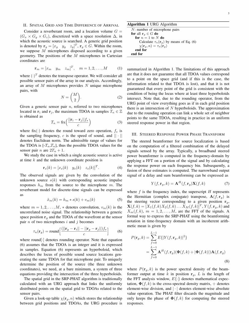
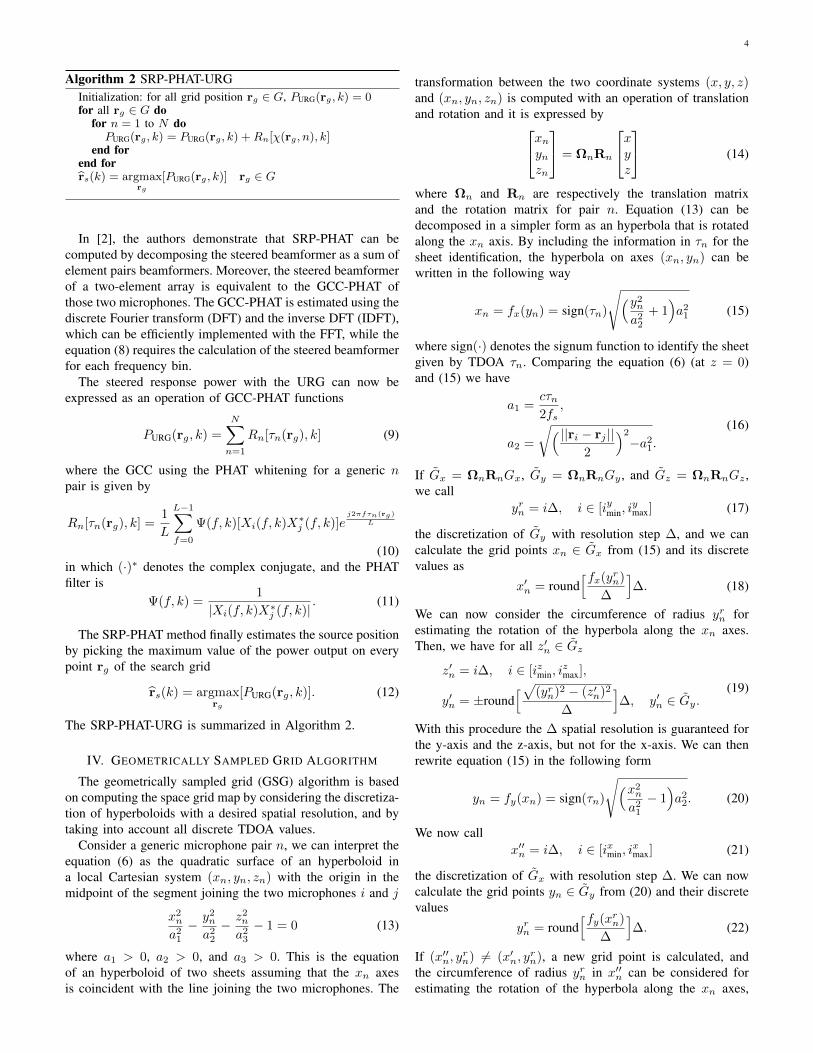
Fig. 1. A discrete hyperbola related to a TDOA τn = −90 samples using theGSG algorithm for a microphone pair ri = [1 1.2]T m and rj = [2 1.8]T
m. For each grid sample position rg of the hyperbola, the values rg , n, andτn are stored in look-up tables γr(q), γn(q) and γτ (q) respectively, and thenumber of hyperbolas passing through position rg are stored in δ(rg). Spaceresolution ∆ is 0.1 m and fs = 44.1 kHz.
obtaining the coordinates (x′′n, y′′n, z′′n). This procedure ensures
that also the x-axis will eventually have spatial resolution ∆.After the transformation of rn = [x′n y′n z′n]T (or
r′n = [x′′n y′′n z′′n]T ) into the coordinate system (x, y, z),we obtain the grid sample position rg = [xg yg zg]
T . Notethat, due to the rounding operator, there are regions where twoor more hyperboloids corresponding to different TDOAs maybe mapped on the same point of the grid. Thus, in contrastto the URG case in which, due to equation (6), there arealways exactly N TDOA values associated to each point onthe grid (one for each microphone pair), the GSG proceduremay associate less than N , N or more than N TDOAs to apoint on the grid. This property is illustrated in Figure 11,for a section of the search space corresponding to a simulatedacoustic environment.
We build the grid map with resolution ∆ for all N mi-crophone pairs and for each pair considering all 2Tn + 1TDOA values. The values of the discrete hyperboloid andthe TDOA information are stored in four look-up tables. Toeach discrete hyperboloid point, we assign an index q, sothat we have a table γr(q) for the position, a table γn(q)for the pair index, and a table γτ (q) for the TDOA. Thetables are used in real-time for estimating the acoustic energyand computing the accumulation of GCC-PHAT functions byall considered sensor pair. We define Q′ as the number ofdiscrete hyperboloid points calculated by the GSG algorithm.The last look-up table, which we name δ(rg), contains theactual number of the surfaces intersecting in position rg .
To be consistent with the definition of a candidate sourceposition as the intersection of hyperboloids, the followingconstraint is applied after the complete analysis of δ(rg) forall rg ∈ G
δ(rg) = 0, if δ(rg) < µ (23)
where µ = 3 and µ = 2 in case of 3D and 2D localizationrespectively. The constraint has the goal to discard those
sample space point that are not consistent for the localization.The inconsistent grid points are eliminated from the look-uptables γr(q), γn(q), and γτ (q) so that all information on thecoherent grid representing the relationship with TDOAs of allpair sensor can be used for the localization. If T is the numberof points which are non consistent with respect to condition(23), then Q = Q′ − T is the number of discrete hyperboloidpoints after their removal. Figure 1 shows a discrete hyperbolarelated to a TDOA tn = −90 samples of a specific microphonepair n. The space resolution is ∆ = 0.1 m, and the area ofanalysis is Gx = 4 m and Gy = 3 m. Blue circles are theidentified grid positions that are stored in the look-up tablesγr(q), γn(q), γτ (q) and δ(rg). The table δ(rg) is the sensitivitymap that gives information on how all sampled GCC-PHATvalues are projected into space. In this way, we can obtain asensitivity map of the considered grid. It will be shown in theexperimental section that an improvement in the localizationaccuracy is obtained in the high sensitivity regions, wherethe accumulation of GCC-PHAT information is higher. Thecoherent grid Γr related to the array is calculated by removingduplicate positions in γr(q)
Γr = unique[γr(q)] (24)
where unique(·) denotes the operator which removes duplicatevalues from a list.
The procedure to build the coherently sampled grid and thesensitivity map in a geometric way is given by the followingsteps:
1) Initialization of δ(rg) = 0 for all rg ∈ G and of indexq=0;
2) For each sensor pair n = 1, 2, . . . , N and for all TDOAvalues τn in the range [-Tn,Tn], calculate the discretehyperboloid, write the values in the look-up tables γr(q),γn(q), and γτ (q), update the value of the look-up tableδ(rg) = δ(rg) + 1, and update q = q + 1;
3) After the geometric discrete analysis of hyperboloids hasterminated, apply the constraint on δ(rg) and update thelook-up tables γr(q), γn(q), and γτ (q).
The GSC algorithm is summarized in Algorithm 3.Finally, at each analysis frame k, the GSG based SRP-
PHAT is computed in three steps. First, the map is initializedby imposing the steered response power PGSG[rg, k] = 0with rg ∈ Γr. Then, the values from the estimated GCC-PHAT functions are accumulated in the grid map. Finally, thesource position is estimated by picking the maximum valueof the acoustic map. The SRP-PHAT-GSG is summarized inAlgorithm 4.
The output of the SRP-PHAT using the GSG algorithm canbe expressed as
PGSG(rg, k) =∑h∈Hr
Rγn(h)[γτ (h), k] (25)
whereHr = i : γr(i) = rg (26)
are the look-up table indices corresponding to the TDOAs forthe position rg ∈ Γr of all the N sensor pairs. Note that Hr is
6
Algorithm 3 GSG AlgorithmN : number of microphone pairs∆: spatial resolutionInitialization: for all grid position rg ∈ G, δ(rg) = 0Initialization: q = 0for n = 1 to N do
Calculate the local coordinate system (xn, yn, zn)Calculate 2Tn + 1 (number of TDOA samples for the nth pair)
for τn = −Tn to Tn dofor all yrn ∈ Gy do
Calculate x′nif x′n ∈ Gx then
for all z′n ∈ Gz doCalculate y′nif y′n ∈ Gy then
Transform rn = [x′n y′n z′n]T to rg =[xg yg zg]
T
γr(q) = rg , γn(q) = n, γτ (q) = τnδ(rg) = δ(rg) + 1q=q+1
end ifend for
end ifend forfor all x′′n ∈ Gx do
Calculate yrnif yrn ∈ Gx and (x′′n, y
rn) 6= (x′n, y
rn) then
for all z′′n ∈ Gz doCalculate y′′nif y′′n ∈ Gy then
Transform r′n = [x′′n y′′n z′′n]T to r′g =[x′g y
′g z
′g]T
γr(q) = r′g , γn(q) = n, γτ (q) = τnδ(r′g) = δ(r′g) + 1q=q+1
end ifend for
end ifend for
end forend forQ’=qApply the constraint and compute TUpdate γr(q), γn(q), and γτ (q)Q=Q’-TΓr = unique[γr(q)]
Algorithm 4 SRP-PHAT-GSGInitialization: for all grid position rg ∈ Γr , PGSG[rg, k] = 0for q = 1 to Q doPGSG[γr(q), k] = PGSG[γr(q), k] +Rγn(q)[γτ (q), k]
end forrs(k) = argmax
rg
(PGSG[rg, k]) rg ∈ Γr
a set of TDOAs of dimension δ(rg). After some manipulationon equation (25), we can write the SRP-PHAT-GSG as
PGSG(rg, k) =
N∑n=1
∑z∈Zr,n
Rn[γτ (z), k] (27)
where
Zr,n = i : [γr(i) = rg] ∧ [γn(i) = n] (28)
are the look-up table indices corresponding to the TDOAs forthe position rg ∈ Γr of the sensor pair n. Note that Zr,nis an empty set if i : [γr(i) = rg] ∧ [γn(i) = n] is null.By comparing equations (9) and (27), we can observe thatfor each position related to the microphone pair n, we canhave a larger amount of TDOA information, which is theprincipal reason of the increased localization performance inthe high sensitivity region. Note that the SRP-PHAT expressedby equation (27) has a similar form of other accumulationmethods [13]–[15]. However, GSG designs a coherent spatialgrid and provides a sensitivity map, which gives informationof how the whole GCC-PHAT information is distributed inthe search space, resulting in different regions characterizedby different localization accuracies.
The computational cost for the GSG algorithm is equivalentto that of the URG procedure for computing the power map,since for both algorithms the relationship between TDOAs andpositions in space is pre-calculated offline using the look-up tables, and online summation is negligible. Consistentreduction of the computational cost may occur for the searchprocedure, which depends on the number of sample gridpositions. If the search procedure is restricted to the coherentgrid, the computational cost is inferior to the URG method dueto the discarded points. Moreover, the computational cost maybe also reduced by using a coarser grid or by only searching inthe high sensitivity regions, in which the localization accuracyis maximized.
V. EXPERIMENTAL RESULTS
A. Spatial Grid and Power Response Sensitivity Analysis
In this section, we present experimental results concerningthe construction of the spatial grid and the analysis of thepower response sensitivity using the GSG algorithm for anuniform linear array (ULA). Spatial grids were designed usingdifferent small-array sizes, sampling rate values, and spatialresolutions. A search region of 2 m × 2 m was considered.Table I shows the resulting number of grid points when usingthe URG and the GSG methods, for an ULA with an inter-microphone distance of 0.15 m. The coverage percentagevalues reported show how the acoustically coherent grid is insome cases much smaller if compared to the uniform regulargrid (especially when using a small array size combined witha high spatial resolution). As already noted, using the coherentspatial grid obtained by the GSG algorithm in those cases, hasthe advantage of providing a position search domain which isconsistent with the hyperboloid intersections, whereas URGgrid would also contain non-consistent regions which wouldprovide misleading information, since the corresponding en-ergy on the search map is usually comparable to that ofconsistent regions.
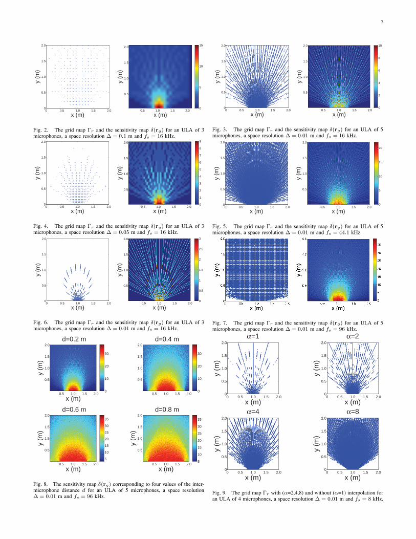
Figures 2, 3, 4, 5, 6, 7 depict the grid map Γr and thesensitivity map δ(rg) calculated with the GSG algorithm fordifferent system configurations. The center of the array ispositioned at location (1,0) m. Note that the δ(rg) tables in thefigures are reported before applying the constraint in equation(23). The colorbar on the right of the figures shows the numberof the intersections of hyperbolas.
7
0 0.5 1.0 1.5 2.00
0.5
1.0
1.5
2.0
x (m)
y (m
)
x (m)y
(m)
0.5 1.0 1.5 2.0
0.5
1.0
1.5
2.0
0
5
10
15
Fig. 2. The grid map Γr and the sensitivity map δ(rg) for an ULA of 3microphones, a space resolution ∆ = 0.1 m and fs = 16 kHz.
0 0.5 1.0 1.5 2.00
0.5
1.0
1.5
2.0
x (m)
y (m
)
x (m)
y (m
)
0.5 1.0 1.5 2.0
0.5
1.0
1.5
2.0
0
2
4
6
8
10
Fig. 3. The grid map Γr and the sensitivity map δ(rg) for an ULA of 5microphones, a space resolution ∆ = 0.01 m and fs = 16 kHz.
0 0.5 1.0 1.5 2.00
0.5
1.0
1.5
2.0
x (m)
y (m
)
x (m)
y (m
)
0.5 1.0 1.5 2.0
0.5
1.0
1.5
2.0
0
1
2
3
4
5
6
7
8
9
Fig. 4. The grid map Γr and the sensitivity map δ(rg) for an ULA of 3microphones, a space resolution ∆ = 0.05 m and fs = 16 kHz.
0 0.5 1.0 1.5 2.00
0.5
1.0
1.5
2.0
x (m)y
(m)
x (m)
y (m
)
0.5 1.0 1.5 2.0
0.5
1.0
1.5
2.0
0
5
10
15
20
Fig. 5. The grid map Γr and the sensitivity map δ(rg) for an ULA of 5microphones, a space resolution ∆ = 0.01 m and fs = 44.1 kHz.
0 0.5 1.0 1.5 2.00
0.5
1.0
1.5
2.0
x (m)
y (m
)
x (m)
y (m
)
0.5 1.0 1.5 2.0
0.5
1.0
1.5
2.0
0
0.5
1
1.5
2
2.5
3
Fig. 6. The grid map Γr and the sensitivity map δ(rg) for an ULA of 3microphones, a space resolution ∆ = 0.01 m and fs = 16 kHz.
Fig. 7. The grid map Γr and the sensitivity map δ(rg) for an ULA of 5microphones, a space resolution ∆ = 0.01 m and fs = 96 kHz.
d=0.2 m
x (m)
y (m
)
0.5 1.0 1.5 2.0
0.5
1.0
1.5
2.0 d=0.4 m
0.5 1.0 1.5 2.0
0.5
1.0
1.5
2.0
d=0.6 m
x (m)
y (m
)
0.5 1.0 1.5 2.0
0.5
1.5
1.5
2.0 d=0.8 m
x (m)
y (m
)
0.5 1.0 1.5 2.0
0.5
1.0
1.5
2.0
5
10
15
20
25
30
35
0
10
20
30
0
10
20
30
5
10
15
20
25
30
35
Fig. 8. The sensitivity map δ(rg) corresponding to four values of the inter-microphone distance d for an ULA of 5 microphones, a space resolution∆ = 0.01 m and fs = 96 kHz.
0 0.5 1.0 1.5 2.00
0.5
1.0
1.5
2.0
x (m)
y (m
)
α=1
0 0.5 1.0 1.5 2.00
0.5
1.0
1.5
2.0
x (m)
y (m
)
α=2
0 0.5 1.0 1.5 2.00
0.5
1.0
1.5
2.0
x (m)
y (m
)
α=4
0 0.5 1.0 1.5 2.00
0.5
1.0
1.5
2.0
x (m)
y (m
)
α=8
Fig. 9. The grid map Γr with (α=2,4,8) and without (α=1) interpolation foran ULA of 4 microphones, a space resolution ∆ = 0.01 m and fs = 8 kHz.
8
TABLE ICOMPARISON OF NUMBER OF GRID POINTS FOR A ULA USING URG AND GSG ALGORITHM.
URG (M=3,4,5,6) GSG (M=3) GSG (M=4) GSG (M=5) GSG (M=6)
fs=16000 Hz ∆ = 0.01 m 40000 (100 %) 486 (1.22 %) 3930 (9.83 %) 10854 (27.14 %) 20242 (50.61 %)∆ = 0.05 m 1600 (100 %) 264 (16.50 %) 1140 (71.25 %) 1446 (90.38 %) 1509 (94.31 %)∆ = 0.1 m 400 (100 %) 185 (46.25 %) 358 (89.50 %) 370 (92.50 %) 374 (93.50 %)
fs=44100 Hz ∆ = 0.01 m 40000 (100 %) 3710 (9.28 %) 15816 (39.54 %) 29708 (74.27 %) 36958 (92.40 %)∆ = 0.05 m 1600 (100 %) 1281 (80.06 %) 1527 (95.44 %) 1540 (96.25 %) 1559 (97.44 %)∆ = 0.1 m 400 (100 %) 372 (93.00 %) 378 (94.50 %) 380 (95.00 %) 380 (95.00 %)
fs=96000 Hz ∆ = 0.01 m 40000 (100 %) 12362 (30.91 %) 31908 (79.77 %) 38358 (95.90 %) 39103 (97.76 %)∆ = 0.05 m 1600 (100 %) 1512 (94.50 %) 1535 (95.94 %) 1548 (96.75 %) 1552 (97.00 %)∆ = 0.1 m 400 (100 %) 374 (93.50 %) 380 (95.00 %) 380 (95.00 %) 380 (95.00 %)
By observing the sensitivity maps, we can see how theGCC-PHAT functions are projected onto the search region,and how their values are accumulated. We note that the redcolored regions are characterized by a high power responsesensitivity since they accommodate a high number of hy-perbola intersections. We can see in Figure 7 that the highsensitivity region accommodates a number of intersectionscontained in the range [25, 35], whereas the URG onlyaccounts for M(M − 1)/2 = 10 intersections at each pointon the grid. Figure 8 depicts the power response sensitivityanalysis corresponding to different values of the array aperture,for an ULA of 5 microphones, a space resolution ∆ = 0.01 mand fs = 96 kHz. We observe how the high sensitivity region(red-colored region) expands when the distance between mi-crophone increases, due to the higher resolution of the GCC-PHAT functions that provide a larger number of hyperbolasfor each sensor pair.
The coherent spatial grid and the sensitivity map can beoptimally constructed for a specific search region by properlyconfiguring the geometry of the array, the number of micro-phones, and the sampling frequency. An alternative way toincrease the TDOA resolution, and accordingly the numberof hyperboloid of a sensor pair, is by interpolation. If 1/α isan upsampling step, the possible TDOA values for the sensorpair n will become 2αTn+1. When interpolation is consideredin the GSG, we have to calculate discrete hyperboloids alsofor non-integer TDOA values according to the parameter α.An example of interpolation in the GSG is shown in Figure9, in which we can observe the spatial grid correspondingto different values of α, for an ULA of 4 microphones, aspace resolution ∆ = 0.01 m and fs = 8 kHz. Note thatthe effectiveness of interpolation for incrementing the spatialresolution is related to the signal-to-noise ratio (SNR) of thesignal, and upsampling may lead to poor accuracy for lowSNR [18].
In next sections, we will see the importance of the powerresponse sensitivity analysis and how it is deeply related tothe performance of sound source localization.
B. Localization Performance for Simulated Data
In this section, the localization performance of the proposedGSG algorithm is assessed on a set of acoustic data simulatednumerically. We also show that the sensitivity map obtained
0 0.5 1 1.5 2 2.5 3 3.5 40
0.5
1
1.5
2
2.5
3
r1
r2
r3
r4
r5
x (m)
y (m
)
Zone B
Zone A
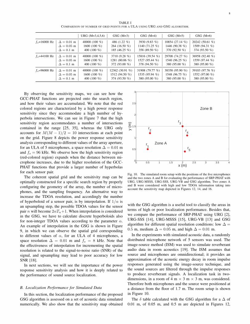
Fig. 10. The simulated room setup with the positions of the five microphonesand the two zones A and B for evaluating the performance of SRP-PHAT withURG, URG-MSSS, URG-SSS, URG-VB and GSG algorithm. Two zones Aand B were considered with high and low TDOA information taking intoaccount the sensitivity map depicted in Figures 12, 14, and 16.
with the GSG algorithm is a useful tool to classify the areas interms of high or poor localization performance. Besides that,we compare the performance of SRP-PHAT using URG [2],URG-SSS [14], URG-MSSS [15], URG-VB [13] and GSGalgorithm for different spatial resolution conditions: low ∆ =0.5 m, medium ∆ = 0.05 m, and high ∆ = 0.01 m.
In the experiments with simulated acoustic data, a randomlydistributed microphone network of 5 sensors was used. Theimage-source method (ISM) was used to simulate reverberantaudio data in room acoustics [19]. The ISM assumes thatsource and microphones are omnidirectional; it provides anapproximation of the acoustic energy decay in room impulseresponses generated using the image-source technique, andthe sound sources are filtered through the impulse responsesto produce reverberant signals. A localization task in two-dimensions, in a room of 4 m × 3 m × 3 m, was considered.Therefore both microphones and the source were positioned ata distance from the floor of 1.7 m. The room setup is shownin Figure 10.
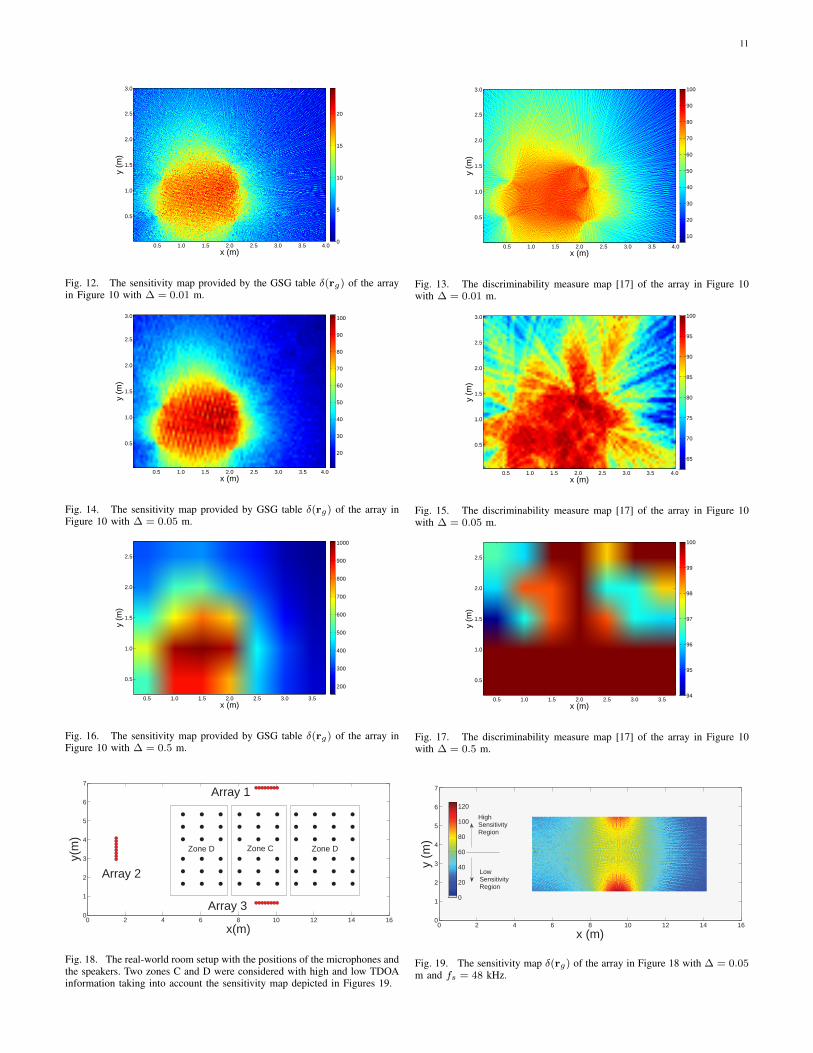
The δ table calculated with the GSG algorithm for a ∆ of0.01 m, of 0.05 m, and 0.5 m are depicted in Figures 12,
9
0 0.5 1.0 1.5 2.0 2.5 3.0 3.5 4.00123456789
10111213141516171819202122232425
x (m)
Num
ber o
f hyp
erbo
la in
ters
ectio
ns
low
sen
sitiv
ity re
gion
high sensitivity region low sensitivity region
non consistent points
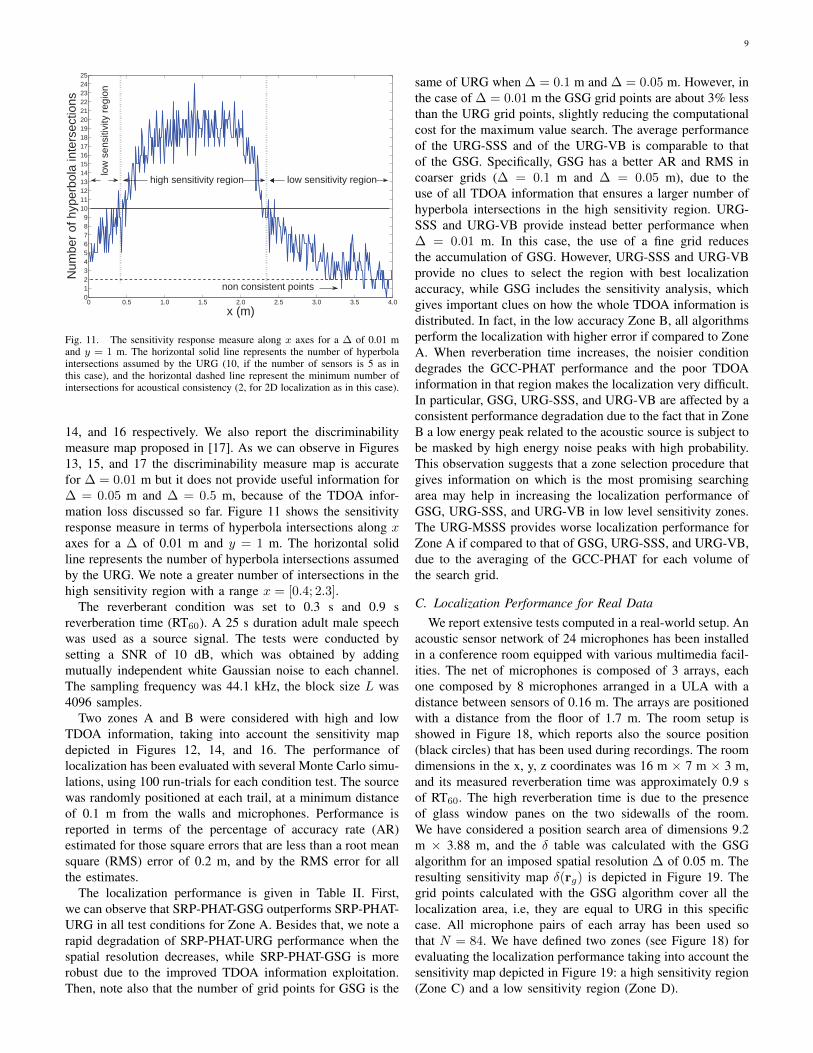
Fig. 11. The sensitivity response measure along x axes for a ∆ of 0.01 mand y = 1 m. The horizontal solid line represents the number of hyperbolaintersections assumed by the URG (10, if the number of sensors is 5 as inthis case), and the horizontal dashed line represent the minimum number ofintersections for acoustical consistency (2, for 2D localization as in this case).
14, and 16 respectively. We also report the discriminabilitymeasure map proposed in [17]. As we can observe in Figures13, 15, and 17 the discriminability measure map is accuratefor ∆ = 0.01 m but it does not provide useful information for∆ = 0.05 m and ∆ = 0.5 m, because of the TDOA infor-mation loss discussed so far. Figure 11 shows the sensitivityresponse measure in terms of hyperbola intersections along xaxes for a ∆ of 0.01 m and y = 1 m. The horizontal solidline represents the number of hyperbola intersections assumedby the URG. We note a greater number of intersections in thehigh sensitivity region with a range x = [0.4; 2.3].
The reverberant condition was set to 0.3 s and 0.9 sreverberation time (RT60). A 25 s duration adult male speechwas used as a source signal. The tests were conducted bysetting a SNR of 10 dB, which was obtained by addingmutually independent white Gaussian noise to each channel.The sampling frequency was 44.1 kHz, the block size L was4096 samples.
Two zones A and B were considered with high and lowTDOA information, taking into account the sensitivity mapdepicted in Figures 12, 14, and 16. The performance oflocalization has been evaluated with several Monte Carlo simu-lations, using 100 run-trials for each condition test. The sourcewas randomly positioned at each trail, at a minimum distanceof 0.1 m from the walls and microphones. Performance isreported in terms of the percentage of accuracy rate (AR)estimated for those square errors that are less than a root meansquare (RMS) error of 0.2 m, and by the RMS error for allthe estimates.
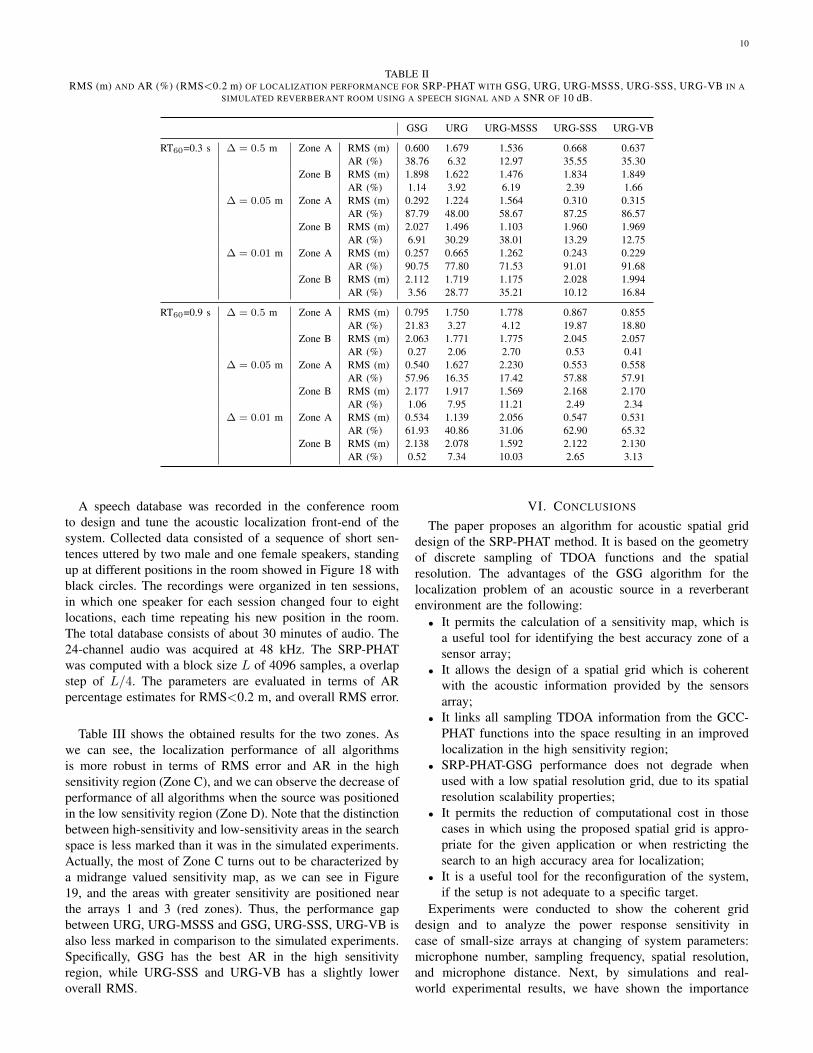
The localization performance is given in Table II. First,we can observe that SRP-PHAT-GSG outperforms SRP-PHAT-URG in all test conditions for Zone A. Besides that, we note arapid degradation of SRP-PHAT-URG performance when thespatial resolution decreases, while SRP-PHAT-GSG is morerobust due to the improved TDOA information exploitation.Then, note also that the number of grid points for GSG is the
same of URG when ∆ = 0.1 m and ∆ = 0.05 m. However, inthe case of ∆ = 0.01 m the GSG grid points are about 3% lessthan the URG grid points, slightly reducing the computationalcost for the maximum value search. The average performanceof the URG-SSS and of the URG-VB is comparable to thatof the GSG. Specifically, GSG has a better AR and RMS incoarser grids (∆ = 0.1 m and ∆ = 0.05 m), due to theuse of all TDOA information that ensures a larger number ofhyperbola intersections in the high sensitivity region. URG-SSS and URG-VB provide instead better performance when∆ = 0.01 m. In this case, the use of a fine grid reducesthe accumulation of GSG. However, URG-SSS and URG-VBprovide no clues to select the region with best localizationaccuracy, while GSG includes the sensitivity analysis, whichgives important clues on how the whole TDOA information isdistributed. In fact, in the low accuracy Zone B, all algorithmsperform the localization with higher error if compared to ZoneA. When reverberation time increases, the noisier conditiondegrades the GCC-PHAT performance and the poor TDOAinformation in that region makes the localization very difficult.In particular, GSG, URG-SSS, and URG-VB are affected by aconsistent performance degradation due to the fact that in ZoneB a low energy peak related to the acoustic source is subject tobe masked by high energy noise peaks with high probability.This observation suggests that a zone selection procedure thatgives information on which is the most promising searchingarea may help in increasing the localization performance ofGSG, URG-SSS, and URG-VB in low level sensitivity zones.The URG-MSSS provides worse localization performance forZone A if compared to that of GSG, URG-SSS, and URG-VB,due to the averaging of the GCC-PHAT for each volume ofthe search grid.
C. Localization Performance for Real DataWe report extensive tests computed in a real-world setup. An
acoustic sensor network of 24 microphones has been installedin a conference room equipped with various multimedia facil-ities. The net of microphones is composed of 3 arrays, eachone composed by 8 microphones arranged in a ULA with adistance between sensors of 0.16 m. The arrays are positionedwith a distance from the floor of 1.7 m. The room setup isshowed in Figure 18, which reports also the source position(black circles) that has been used during recordings. The roomdimensions in the x, y, z coordinates was 16 m × 7 m × 3 m,and its measured reverberation time was approximately 0.9 sof RT60. The high reverberation time is due to the presenceof glass window panes on the two sidewalls of the room.We have considered a position search area of dimensions 9.2m × 3.88 m, and the δ table was calculated with the GSGalgorithm for an imposed spatial resolution ∆ of 0.05 m. Theresulting sensitivity map δ(rg) is depicted in Figure 19. Thegrid points calculated with the GSG algorithm cover all thelocalization area, i.e, they are equal to URG in this specificcase. All microphone pairs of each array has been used sothat N = 84. We have defined two zones (see Figure 18) forevaluating the localization performance taking into account thesensitivity map depicted in Figure 19: a high sensitivity region(Zone C) and a low sensitivity region (Zone D).
10
TABLE IIRMS (m) AND AR (%) (RMS<0.2 m) OF LOCALIZATION PERFORMANCE FOR SRP-PHAT WITH GSG, URG, URG-MSSS, URG-SSS, URG-VB IN A
SIMULATED REVERBERANT ROOM USING A SPEECH SIGNAL AND A SNR OF 10 dB.
GSG URG URG-MSSS URG-SSS URG-VB
RT60=0.3 s ∆ = 0.5 m Zone A RMS (m) 0.600 1.679 1.536 0.668 0.637AR (%) 38.76 6.32 12.97 35.55 35.30
Zone B RMS (m) 1.898 1.622 1.476 1.834 1.849AR (%) 1.14 3.92 6.19 2.39 1.66
∆ = 0.05 m Zone A RMS (m) 0.292 1.224 1.564 0.310 0.315AR (%) 87.79 48.00 58.67 87.25 86.57
Zone B RMS (m) 2.027 1.496 1.103 1.960 1.969AR (%) 6.91 30.29 38.01 13.29 12.75
∆ = 0.01 m Zone A RMS (m) 0.257 0.665 1.262 0.243 0.229AR (%) 90.75 77.80 71.53 91.01 91.68
Zone B RMS (m) 2.112 1.719 1.175 2.028 1.994AR (%) 3.56 28.77 35.21 10.12 16.84
RT60=0.9 s ∆ = 0.5 m Zone A RMS (m) 0.795 1.750 1.778 0.867 0.855AR (%) 21.83 3.27 4.12 19.87 18.80
Zone B RMS (m) 2.063 1.771 1.775 2.045 2.057AR (%) 0.27 2.06 2.70 0.53 0.41
∆ = 0.05 m Zone A RMS (m) 0.540 1.627 2.230 0.553 0.558AR (%) 57.96 16.35 17.42 57.88 57.91
Zone B RMS (m) 2.177 1.917 1.569 2.168 2.170AR (%) 1.06 7.95 11.21 2.49 2.34
∆ = 0.01 m Zone A RMS (m) 0.534 1.139 2.056 0.547 0.531AR (%) 61.93 40.86 31.06 62.90 65.32
Zone B RMS (m) 2.138 2.078 1.592 2.122 2.130AR (%) 0.52 7.34 10.03 2.65 3.13
A speech database was recorded in the conference roomto design and tune the acoustic localization front-end of thesystem. Collected data consisted of a sequence of short sen-tences uttered by two male and one female speakers, standingup at different positions in the room showed in Figure 18 withblack circles. The recordings were organized in ten sessions,in which one speaker for each session changed four to eightlocations, each time repeating his new position in the room.The total database consists of about 30 minutes of audio. The24-channel audio was acquired at 48 kHz. The SRP-PHATwas computed with a block size L of 4096 samples, a overlapstep of L/4. The parameters are evaluated in terms of ARpercentage estimates for RMS<0.2 m, and overall RMS error.
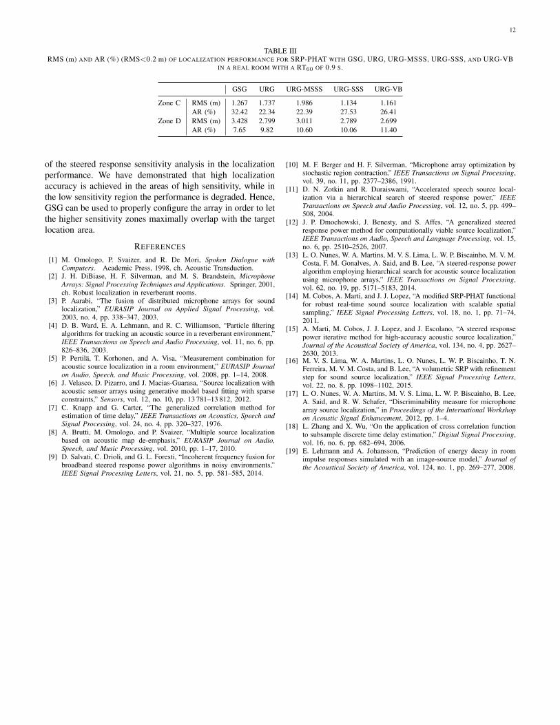
Table III shows the obtained results for the two zones. Aswe can see, the localization performance of all algorithmsis more robust in terms of RMS error and AR in the highsensitivity region (Zone C), and we can observe the decrease ofperformance of all algorithms when the source was positionedin the low sensitivity region (Zone D). Note that the distinctionbetween high-sensitivity and low-sensitivity areas in the searchspace is less marked than it was in the simulated experiments.Actually, the most of Zone C turns out to be characterized bya midrange valued sensitivity map, as we can see in Figure19, and the areas with greater sensitivity are positioned nearthe arrays 1 and 3 (red zones). Thus, the performance gapbetween URG, URG-MSSS and GSG, URG-SSS, URG-VB isalso less marked in comparison to the simulated experiments.Specifically, GSG has the best AR in the high sensitivityregion, while URG-SSS and URG-VB has a slightly loweroverall RMS.
VI. CONCLUSIONS
The paper proposes an algorithm for acoustic spatial griddesign of the SRP-PHAT method. It is based on the geometryof discrete sampling of TDOA functions and the spatialresolution. The advantages of the GSG algorithm for thelocalization problem of an acoustic source in a reverberantenvironment are the following:• It permits the calculation of a sensitivity map, which is
a useful tool for identifying the best accuracy zone of asensor array;
• It allows the design of a spatial grid which is coherentwith the acoustic information provided by the sensorsarray;
• It links all sampling TDOA information from the GCC-PHAT functions into the space resulting in an improvedlocalization in the high sensitivity region;
• SRP-PHAT-GSG performance does not degrade whenused with a low spatial resolution grid, due to its spatialresolution scalability properties;
• It permits the reduction of computational cost in thosecases in which using the proposed spatial grid is appro-priate for the given application or when restricting thesearch to an high accuracy area for localization;
• It is a useful tool for the reconfiguration of the system,if the setup is not adequate to a specific target.
Experiments were conducted to show the coherent griddesign and to analyze the power response sensitivity incase of small-size arrays at changing of system parameters:microphone number, sampling frequency, spatial resolution,and microphone distance. Next, by simulations and real-world experimental results, we have shown the importance
11
x (m)
y (m
)
0.5 1.0 1.5 2.0 2.5 3.0 3.5 4.0
0.5
1.0
1.5
2.0
2.5
3.0
0
5
10
15
20
Fig. 12. The sensitivity map provided by the GSG table δ(rg) of the arrayin Figure 10 with ∆ = 0.01 m.
x (m)
y (m
)
0.5 1.0 1.5 2.0 2.5 3.0 3.5 4.0
0.5
1.0
1.5
2.0
2.5
3.0
10
20
30
40
50
60
70
80
90
100
Fig. 13. The discriminability measure map [17] of the array in Figure 10with ∆ = 0.01 m.
x (m)
y (m
)
0.5 1.0 1.5 2.0 2.5 3.0 3.5 4.0
0.5
1.0
1.5
2.0
2.5
3.0
20
30
40
50
60
70
80
90
100
Fig. 14. The sensitivity map provided by GSG table δ(rg) of the array inFigure 10 with ∆ = 0.05 m.
x (m)y
(m)
0.5 1.0 1.5 2.0 2.5 3.0 3.5 4.0
0.5
1.0
1.5
2.0
2.5
3.0
65
70
75
80
85
90
95
100
Fig. 15. The discriminability measure map [17] of the array in Figure 10with ∆ = 0.05 m.
x (m)
y (m
)
0.5 1.0 1.5 2.0 2.5 3.0 3.5
0.5
1.0
1.5
2.0
2.5
200
300
400
500
600
700
800
900
1000
Fig. 16. The sensitivity map provided by GSG table δ(rg) of the array inFigure 10 with ∆ = 0.5 m.
x (m)
y (m
)
0.5 1.0 1.5 2.0 2.5 3.0 3.5
0.5
1.0
1.5
2.0
2.5
94
95
96
97
98
99
100
Fig. 17. The discriminability measure map [17] of the array in Figure 10with ∆ = 0.5 m.
0 2 4 6 8 10 12 14 160
1
2
3
4
5
6
7
x(m)
y(m
)
Array 2
Zone D Zone D
Array 1
Array 3
Zone C
Fig. 18. The real-world room setup with the positions of the microphones andthe speakers. Two zones C and D were considered with high and low TDOAinformation taking into account the sensitivity map depicted in Figures 19.
x (m)
y (m
)
0 2 4 6 8 10 12 14 160
1
2
3
4
5
6
7
0
20
40
60
80
100
120
LowSensitivityRegion
HighSensitivityRegion
Fig. 19. The sensitivity map δ(rg) of the array in Figure 18 with ∆ = 0.05m and fs = 48 kHz.
12
TABLE IIIRMS (m) AND AR (%) (RMS<0.2 m) OF LOCALIZATION PERFORMANCE FOR SRP-PHAT WITH GSG, URG, URG-MSSS, URG-SSS, AND URG-VB
IN A REAL ROOM WITH A RT60 OF 0.9 S.
GSG URG URG-MSSS URG-SSS URG-VB
Zone C RMS (m) 1.267 1.737 1.986 1.134 1.161AR (%) 32.42 22.34 22.39 27.53 26.41
Zone D RMS (m) 3.428 2.799 3.011 2.789 2.699AR (%) 7.65 9.82 10.60 10.06 11.40
of the steered response sensitivity analysis in the localizationperformance. We have demonstrated that high localizationaccuracy is achieved in the areas of high sensitivity, while inthe low sensitivity region the performance is degraded. Hence,GSG can be used to properly configure the array in order to letthe higher sensitivity zones maximally overlap with the targetlocation area.
REFERENCES
[1] M. Omologo, P. Svaizer, and R. De Mori, Spoken Dialogue withComputers. Academic Press, 1998, ch. Acoustic Transduction.
[2] J. H. DiBiase, H. F. Silverman, and M. S. Brandstein, MicrophoneArrays: Signal Processing Techniques and Applications. Springer, 2001,ch. Robust localization in reverberant rooms.
[3] P. Aarabi, “The fusion of distributed microphone arrays for soundlocalization,” EURASIP Journal on Applied Signal Processing, vol.2003, no. 4, pp. 338–347, 2003.
[4] D. B. Ward, E. A. Lehmann, and R. C. Williamson, “Particle filteringalgorithms for tracking an acoustic source in a reverberant environment,”IEEE Transactions on Speech and Audio Processing, vol. 11, no. 6, pp.826–836, 2003.
[5] P. Pertila, T. Korhonen, and A. Visa, “Measurement combination foracoustic source localization in a room environment,” EURASIP Journalon Audio, Speech, and Music Processing, vol. 2008, pp. 1–14, 2008.
[6] J. Velasco, D. Pizarro, and J. Macias-Guarasa, “Source localization withacoustic sensor arrays using generative model based fitting with sparseconstraints,” Sensors, vol. 12, no. 10, pp. 13 781–13 812, 2012.
[7] C. Knapp and G. Carter, “The generalized correlation method forestimation of time delay,” IEEE Transactions on Acoustics, Speech andSignal Processing, vol. 24, no. 4, pp. 320–327, 1976.
[8] A. Brutti, M. Omologo, and P. Svaizer, “Multiple source localizationbased on acoustic map de-emphasis,” EURASIP Journal on Audio,Speech, and Music Processing, vol. 2010, pp. 1–17, 2010.
[9] D. Salvati, C. Drioli, and G. L. Foresti, “Incoherent frequency fusion forbroadband steered response power algorithms in noisy environments,”IEEE Signal Processing Letters, vol. 21, no. 5, pp. 581–585, 2014.
[10] M. F. Berger and H. F. Silverman, “Microphone array optimization bystochastic region contraction,” IEEE Transactions on Signal Processing,vol. 39, no. 11, pp. 2377–2386, 1991.
[11] D. N. Zotkin and R. Duraiswami, “Accelerated speech source local-ization via a hierarchical search of steered response power,” IEEETransactions on Speech and Audio Processing, vol. 12, no. 5, pp. 499–508, 2004.
[12] J. P. Dmochowski, J. Benesty, and S. Affes, “A generalized steeredresponse power method for computationally viable source localization,”IEEE Transactions on Audio, Speech and Language Processing, vol. 15,no. 6, pp. 2510–2526, 2007.
[13] L. O. Nunes, W. A. Martins, M. V. S. Lima, L. W. P. Biscainho, M. V. M.Costa, F. M. Gonalves, A. Said, and B. Lee, “A steered-response poweralgorithm employing hierarchical search for acoustic source localizationusing microphone arrays,” IEEE Transactions on Signal Processing,vol. 62, no. 19, pp. 5171–5183, 2014.
[14] M. Cobos, A. Marti, and J. J. Lopez, “A modified SRP-PHAT functionalfor robust real-time sound source localization with scalable spatialsampling,” IEEE Signal Processing Letters, vol. 18, no. 1, pp. 71–74,2011.
[15] A. Marti, M. Cobos, J. J. Lopez, and J. Escolano, “A steered responsepower iterative method for high-accuracy acoustic source localization,”Journal of the Acoustical Society of America, vol. 134, no. 4, pp. 2627–2630, 2013.
[16] M. V. S. Lima, W. A. Martins, L. O. Nunes, L. W. P. Biscainho, T. N.Ferreira, M. V. M. Costa, and B. Lee, “A volumetric SRP with refinementstep for sound source localization,” IEEE Signal Processing Letters,vol. 22, no. 8, pp. 1098–1102, 2015.
[17] L. O. Nunes, W. A. Martins, M. V. S. Lima, L. W. P. Biscainho, B. Lee,A. Said, and R. W. Schafer, “Discriminability measure for microphonearray source localization,” in Proceedings of the International Workshopon Acoustic Signal Enhancement, 2012, pp. 1–4.
[18] L. Zhang and X. Wu, “On the application of cross correlation functionto subsample discrete time delay estimation,” Digital Signal Processing,vol. 16, no. 6, pp. 682–694, 2006.
[19] E. Lehmann and A. Johansson, “Prediction of energy decay in roomimpulse responses simulated with an image-source model,” Journal ofthe Acoustical Society of America, vol. 124, no. 1, pp. 269–277, 2008.
Recommended